Embed Size (px)
Citation preview

Mathematical modelling of selected reactions in low-temperature transformation of biomass
Tapio Salmi Åbo Akademi Turku/Åbo Finland


Millireactor technology in the transformation of biomass – hydrolysis of hemicelluloses

Polysaccharides – where?

Why reaction engineering of hemicelluloses?
Ø Hemicelluloses are rich sources of biomass-based products Ø The key issue is the hydrolysis of hemicelluloses to sugar
monomers (homogeneous, enzymatic and heterogeneous catalysis)
Ø The very important products of hemicellulose sugars are obtained by catalytic hydrogenation to sugar alcohols
Ø Valuable products are obtained by oxidation of the monomers to sugar acids

Extraction
H2O, T
Long chained hemicelluloses
Medium and short chained hemicelluloses
Emulsifiers, Films etc.
Platform chemicals
Further processing
Filtration
Oxidation Hydrogenation Fermentation Esterification
Aqueous reforming
Sugar acids, Sugar alcohols, Lubricants, Fuels etc.
< 10 kDa
10 kDa <

Typical hemicelluloses
Ø O-Acetylgalactoglucomannan (mostly mannose units) Ø Arabinogalactan (main chain galactose units) O-Acetyl-(4-O-methylglucurono)xylan (mostly xylose units)

Hemicellulose Monomers
Sugar alcohols
Sugar acids
Hydrolysis
O2, Cat
H2, Cat
From hemicelluloses to chemicals

A hemicellulose to hydrolysis
O-Acetylgalactoglucomannane - a branched hemicellulose (GGM)
Hydrolysed with the aid of homogeneous and heterogeneous catalysts

A hemicellulose: O-acetylgalactoglucomannan

Heterogeneous catalysts
Ø Amberlyst 15: strong sulfonic cation exchange resin
Ø Macroreticular: d=0.45-0.60 mm, pores 40-90 nm
Ø Resin composed of styrene-divinyl benzene with sulfonic acid functional group
Ø Capacity 4.7 mmoleq/g
200 µm

Heterogeneous catalysts
Ø Smopex-101
Ø Fibrous and non-porous: d=0.01 mm I=4 mm
Ø Polymer, polyethene-graft-polystyrene with sulfonic acid functional group
Ø Capacity 3.6 mmoleq/g
20 µm

Hydrolysis experiments I
Ø Batch stirred reactor
Ø Catalysts: HCI, H2SO4, CF3CO2H
Ø Reaction conditions – pH (0.5 - 3) – T (50 - 100°C)
Ø Analysis – Silylation, GC-FID – Molar weight, HPSEC-MALLS

Hydrolysis experiments II
Ø Continuous tube reactor
Ø Catalysts: HCI
Ø Reaction conditions – pH (0.2-0.3) – T (90-95°C)
Ø Analysis – Silylation, GC-FID – Molar weight, HPSEC-MALLS

Continuous tube reactor in laboratory scale

Continuous reactor system schematically

Batch reactor -HCl catalysis
0 200 400 600 800 1000 1200 1400 16000
200
400
600
800
1000
Glucose
Galactose
c
[mg/
g GG
M]
Time [min]
Mannose

Batch reactor - oligomers Molar mass distribution
0 200 400 600 800 1000 1200 1400 16000
200
400
600
800
1000
DP 2 DP 3 DP 4DP 5
c
[mg/
g GG
M]
Time [min]
DP 1

Performance of continuous reactor - monomers

Performanc eof continuous reactor - monomers

Performance of continuous reactor - oligomers

Autocatalysis detected
0 500 1000 1500 2000 2500 3000 3500 4000 45000
50
100
150
200
250
300
350
400
450 data set 1
Heterogeneous catalyst (Smopex)
Mannose
Glucose&Galactose

Heterogeneous catalysis Logarithmic plots
0,00 0,25 0,50 0,75 1,000,00
0,25
0,50
0,75
1,00
-ln(1
-cM/c0M
)
-ln(1-cGA/c0GA)
Smopex-101 Amberlyst 15

Heterogeneous catalyst
0,00 0,25 0,50 0,75 1,000,00
0,25
0,50
0,75
1,00
-ln(1
-cG/c
0G)
-ln(1-cGA/c0GA)
Smopex-101 Amberlyst 15
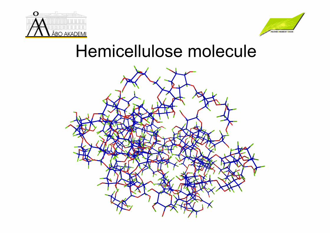
Hemicellulose molecule

Change of rate constant γAXdXdk =/1
0 1+
+=− γ
γXAkk
10 +=−∞ γAkk
αXkkkk )( 00 −+= ∞
)1(0αβXkk jj +=
The increase of the rate constant
(21)
β=(k∞j-k0j)/k0j is constant for all of the sugar units.

Mass balance in batch reactor
j
j
MGGA
MGGA
c
cccccccX
0000 ∑∑=
++
++=
BiWHii ccckdtdc ρ0/ =
jWW ccc ∑−= 0 iii ccc −= 00
Total conversion (X)

Mass balances...
)1(0
0
α
β ⎟⎟
⎠
⎞
⎜⎜
⎝
⎛+=∑∑
j
jii c
ckk
BiijWHj
jii ccccc
c
ckdtdc ρβ
α
))(()1(/ 000
0 −−⎟⎟
⎠
⎞
⎜⎜
⎝
⎛+= ∑∑
∑
which is solved numerically during parameter estimation

Fit of the model for autocatalysis
0 500 1000 1500 2000 2500 3000 3500 4000 45000
50
100
150
200
250
300
350
400
450 data set 1

Modelling of tube reactor
30
- Tubular reactor - laminar flow model, liquid phase only - Convection, both axial and radial diffusion - Dynamic model - Implementation in gProms (Russo & Kilpiö)

Laminar flow model
31
Mass balance
⎥⎥⎦
⎤
⎢⎢⎣
⎡⎟⎠
⎞⎜⎝
⎛−⋅=2
0 1)(Rruru
AVuuu!
=⋅= ,5.10
Liquid velocity and average outlet concentration
∫
∫
⋅⋅⋅
⋅⋅⋅⋅
= R
R
i
i
drrru
drrrurzcc
0
0
2)(
2)(),(
π
π
z
r
),,(),,(1),,(
),,(),,()(),,(
2
2
,
2
2
,
rztrrrztC
rrrztCD
zrztCD
zrztCru
trztC
jiii
ir
iiz
ii
⋅+⎟⎟⎠
⎞⎜⎜⎝
⎛
∂
∂⋅+
∂
∂⋅+
+∂
∂⋅+
∂
∂⋅+=
∂
∂
ν
Accumulation Convection Axial diffusion
Radial diffusion Reactions

Laminar flow model
32
Mass balance
),,(),,(1),,(),,(),,()(),,(2
2
,2
2
, rztrrrztC
rrrztCD
zrztCD
zrztCru
trztC
jiii
iri
izii ⋅+⎟⎟
⎠
⎞⎜⎜⎝
⎛
∂
∂⋅+
∂
∂⋅+
∂
∂⋅+
∂
∂⋅+=
∂
∂ν
Accumulation Convection Axial diffusion Radial diffusion Reaction rate
Boundary conditions
)),(()(),(00,
0, =
=
−⋅=∂
∂⋅−
ziiz
iiz rtCCru
zrtCD 0),(
=∂
∂
=Lz
i
zrtC
Inlet: Outlet:
0),(
0
=∂
∂
=r
i
rztC 0),(
=∂
∂
=Rr
i
rztC
Centre: Wall:
GWH
GAWH
MWH
CCCkrCCCkrCCCkr
⋅⋅⋅=
⋅⋅⋅=
⋅⋅⋅=
33
22
11
Reaction rate expressions

Rate constants from continuous experiments
- good agreement with batch data
Experiment
k’’Gal [min-1]
k’’Glc [min-1]
k’’Man [min-1]
Σk’’i [min-1]
Σk’’i /10-pH
[L/mol/min] Exp I 0.00593 0.00339 0.00608 0.0154 0.031 Exp II 0.00676 0.00452 0.00717 0.0185 0.032 Exp III 0.00576 0.00688 0.01147 0.0241 0.048

Conclusions Homogeneous hydrolysis kinetics of hemicelluloses follows a very regular pattern,except an initiation period Heterogenous hydrolysis kinetics shows a remarkable autocatalytic effect A kinetic model was proposed an successully applied to explain the autocatalysis Hydrolysis can successfully be carried out in continuous mode – good agreement of rate constants compared to batch experiments Laminar flow model is good for the millireactor

Mathematical modelling of cellulose substitution
kinetics

Anhydroglucose units of cellulose C2, C3, C6
O
OH
OOH
OH
OO
OH
OH
OH
O
OH
OH
OH
OH
n
HO
1
2
3
45
6

Experimental approach Isothermal, well-controlled experiments in a slurry batch reactor Cellulose from birch was used, swelled in NaOH and let to react with monochloroacetic acid in isopropanol A lot of effort was put on the development of a new chromatographic method to reveal the detailed substitution kinetics, not only the overall degree of substitution (DS); Substituted units 2, 3, 6, 23, 26, 36 and 236 revealed

Modelling approach Incorporate as much mathematical modelling as possible Everything can be transformed to differential equations, enjoy it! Wood chemistry is not a pure empirical science

Reaction scheme Several substitution reactions
0
3
6 236
2
23
36
26 2k
6k
3k
0
33
6cc
ekδ−
⋅
0
33
2cc
ekδ−
⋅
0
66
3cc
ekδ−
⋅
0
66
2cc
ekδ−
⋅
0
22
6cc
ekδ−
⋅
( )0
2332
6cc
ekδδ +−
⋅
( )0
3663
2cc
ekδδ +−
⋅
( )0
2662
3cc
ekδδ +−
⋅
0
22
3cc
ekδ−
⋅

Substitution reactions
Cell-OH + RCOOH → RCOO-Cell + H2O M+Cell-O- + RX → Cell-OR + M+X- RX=CH3Cl R=CH3CH2Cl

CMC, ethene and propene oxides
M+Cell-O- + CH2ClCOOH → Cell-OCH2COOH + M+Cl-. Cell-OH +HO-R-O- → HO-R-O-Cell + OH- R=CH2CH2 and R=CH2CH2CH2 for ethene and propene oxides

Substitution stoichiometry
663322
PROHPROHPROH
→+
→+
→+
0060302 cccc ===
0ccc Pii =+
Substitution reactions to OH-2, OH-3 and OH-6
R is a substitution reagent and P2, P3 and P6 are product molecules.
ci unsubstituted H-groups, cPi substituted groups (i=2,3,6).

Product formation
α
α
α
RP
RP
RP
cckr
cckr
cckr
666
333
222
=
=
=
PjPPPRR cccccc ∑=++=− 6320
Formation rates
cR = concentration of the substitution reagent Reaction stoichiometry

Batch reactor
PiPi rdtdc =/
Pii ccc −= 0
PjRR ccc ∑−= 0
Mass balances of the product groups in a batch reactor
i=2,3,6.
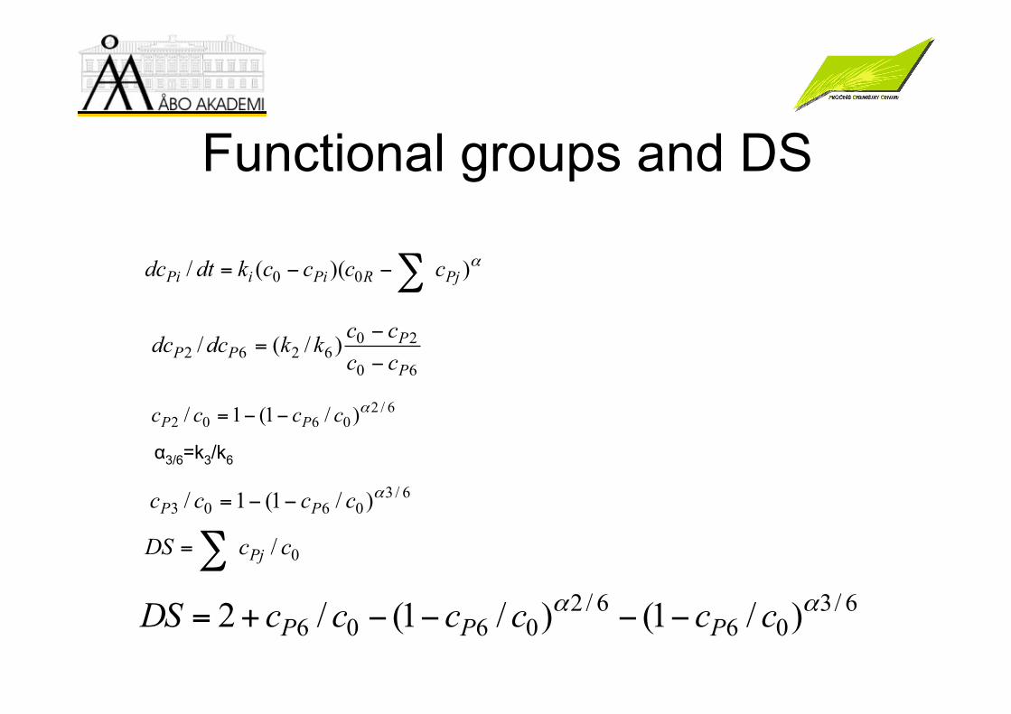
Functional groups and DS
α))((/ 00 PjRPiiPi cccckdtdc ∑−−=
60
206262 )/(/
P
PPP cc
cckkdcdc−
−=
6/20602 )/1(1/ αcccc PP −−=
6/30603 )/1(1/ αcccc PP −−=
0/ ccDS Pj∑=6/3
066/2
0606 )/1()/1(/2 αα ccccccDS PPP −−−−+=
α3/6=k3/k6

DS analytically
tka
tka
eaeaDS ')3(
')3(
)3/(1)1(
−
−
−
−=
)'31'3(3tktkDS
+=
kiteDS −∑−= 3 )1(3 'tkeDS −−=
Second order kinetics and equal reactivities
First and pseudo-first order kinetics
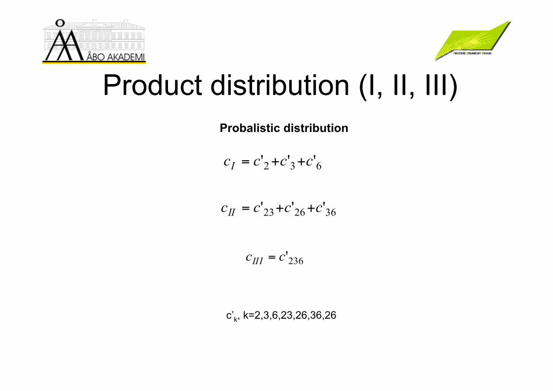
Product distribution (I, II, III)
632 ''' ccccI ++=
362623 ''' ccccII ++=
236'ccIII =
Probalistic distribution
c’k, k=2,3,6,23,26,36,26

Probabilistic distribution
)/)(/1)(/1()/1)(/)(/1()/1)(/1)(/(/ 0603020603020603020 cccccccccccccccccccc PPPPPPPPPI −−+−−+−−=
)/)(/)(/1()/)(/1)(/()/1)(/)(/(/ 0603020603020603020 cccccccccccccccccccc PPPPPPPPPII −+−+−=
)/)(/)(/(/ 0603020 cccccccc PPPIII =
)/1)(/1)(/1(/' 06030200 cccccccc PPP −−−=
000 /3/2/ ccccccDS IIIIII ++=

DS for equal reactivities
300'
30
20
20
)1(/
/
)1(3/
)1(3/
xcc
xcc
xxcc
xxcc
III
II
I
−=
=
−=
−=
nnnn DSDScc −−= 3
0 )3/1()3/(/ γ
Spurlin distribution is obtained
where n=0,I,II,III. γn are obtained from Pascal’s triangle:
γn=(3n)=3!/n!/(3-n)!, n=0,,2,3.

Detailed product distribution ii rdtdc =/'
αRcckkkr 06320 ')( ++−=
αRcckkckr )')('( 263022 +−−=
αRcckkckr )')('( 362033 +−−=
αRcckkckr )')('( 632066 +−−=
αRcckckckr )'''( 236233223 −+=
αRcckckckr )'''( 263266226 −+=
αRcckckckr )'''( 362366336 −+=
αRcckckckr )'''( 236263362236 −+=
i = 0, 2,3, 6, 23,…236, R. Generation rates of different anhydroglucose units:

Kinetics and retardation
αRR cckckckckkckkckkckkkr )'''')(')(')(')(( 2362633626323622630632 +++++++++++−=
DSjj ekk ⋅−= 00
δ
0/0
ccjj
Pkkekk ⋅−∑=δ
Substitution reagent
Retardation functions

Special case
II kckcdtdcdtdcdtdcdtdc 23//// 0632 −==++
IIIII kckcdtdcdtdcdtdcdtdc 22//// 362623 −==++
IIIII kcdtdcdtdc 2//236 ==
00 3/ kcdtdc =
First order kinetics and equally reactive hydroxyl
groups

00 '3/' cddc −=θ
II ccddc 2'3/ 0−=θ
IIIII ccddc −= 2/ θ
IIIII cddc =θ/
Damköhler number, θ=kt:
Solution method

In time scale
θ300 /'
−= eccθθ 2
0 )1(3/' −−−= eecc Iθθθθθ −−−−− −=+−= eeeeecc II
220 )1(3)21(3/'
3320 )1(331/' θθθθ −−−− −=−+−= eeeecc III
)1(3 θ−−= eDS
The solution is easy:

Relative product distribution
632
02632
0
2 )'/')((''
kkkcckkk
dcdc
++
++−=
1)/'('/' 20002 −= −αcccc
)/')(1)/'(('/' 002
0002 cccccc −= −α
Relative product distribution – general approach
X=c’0/c0

The solution
XXcc )1(/' 202 −= −α
XXcc )1(/' 303 −= −α
XXcc )1(/' 606 −= −α
αi= ki/Σkj.

The solution
0632
2362332
0
23
')('''
''
ckkkckckck
dcdc
++
+−−=
31216023 /'
ααα −− −−+= XXXXcc61213
026 /'ααα −− −−+= XXXXcc61312
036 /'ααα −− −−+= XXXXcc

I, II and III
XXXXccI 3/ 6131210 −++= −−− ααα
)(23/ 6131216320
αααααα −−− ++−+++= XXXXXXXccII613121632
0 1/ αααααα −−− +++−−−−= XXXXXXXccIII
)(3 632 ααα XXXDS ++−=

Relative product distribution Equal reactivities of OH-groups
0 0.5 1 1.5 2 2.5 30
0.2
0.4
0.6
0.8
1
Degree of substitution, DS
Mol
e fra
ctio
n
unsubstitutedglucose,
x0
monosubstitutedglucose,
xI
disubstitutedglucose,
xII
trisubstitutedglucose,
xIIIk2:k3:k6 = 1:1:1

Relative product distribution Non-equal reactivities
0 0.5 1 1.5 2 2.5 30
0.2
0.4
0.6
0.8
1
Degree of substitution, DS
Mol
e fra
ctio
n
1:10:10
1:10:10
1:10:10
1:10:10
1:1:10 1:1:10
1:1:10
1:1:10k2:k3:k6

Parameter estimation
)(/ yfdtdy =
( )∑∑ −=t
titii
yyQ 2,exp,,

Experimental product distribution
High-pH AEC-PAD Monomer Distribution (mol%) DS = 0.2 DS = 0.7 Glucose (1) 76.6 34.6 6-O-CM-glucose (2) 12.4 16.8 2-O-CM-glucose (3) 4.2 18.8 3-O-CM-glucose (4) 6.8 24.4 2,6-di-O-CM-glucose (5) 0 2.4 3,6-di-O-CM-glucose (6) 0 1.6 2,3-di-O-CM-glucose (7) 0 1.5 2,3,6-tri-O-CM-glucose 0 0

5,0 5,5 6,0 6,5 7,0 7,5
40
60
80
100
D
etec
tor r
espo
nse
(nC
)
Time (min)
34
2 Fig. 2 C
line B
line A
titration and by HPAEC-PAD.
Carboxymethylation at 30oC (20 min 120 min) 2= 6-O-CM-glucose, 3=2-O-CM-glucose, 4=3-O-CM-glucose
Experimental product distribution (I)

titration and by HPAEC-PAD.
Carboxymethylation at 30oC (20 min, 120 min) 5= 2,6-di-O-CM-glucose, 6=3,6-di-O-CM-glucose, 7=2,3-di-O-CM-glucose
Experimental product distribution (II)
10 11 12 13 1444
45
46
47
48
49
50
Det
ecto
r res
pons
e (n
C)
Time (min)
Fig. 2 D5
67
line A
line B

Estimated kinetic parameters
)
0/)'/(,
0, ccDSRErefjj
Pkkja eeekk ⋅−⋅−− ∑=δδθ
.
Parameter Parameter unit Estimated parameter
value Estimated relative standard error (%)
k2,ref = k3,ref l/(mol min) 0.238 46.4 k6,ref l/(mol min) 0.326 46.5 δ2 - 2.03 52.3 δ3 - 4.42 22.6 δ6 - 6.46 23.5 Ea,2 = Ea,3 kJ/mol 140 11.5 Ea,6 kJ/mol 127 12.5 δ0 - 4.79 14.8

Degree of substitution (DS) Experiment and modelling
0 20 40 60 80 1000
0.5
1
1.5
Time / [min]
Deg
ree
of s
ubst
itutio
n, D
S

Product distribution Unsubstituted, mono-, di- and tri-
substituted units (30oC)
0 20 40 60 80 100 1200
0.2
0.4
0.6
0.8
1
Time / [min]
Mol
e fra
ctio
n

Product distribution Unsubstituted & I & II & III (40oC)
0 20 40 60 80 1000
0.2
0.4
0.6
0.8
1
Time / [min]
Mol
e fra
ctio
n

Product distribution Unsubstituted & I & II & III (60oC)
0 20 40 60 80 1000
0.2
0.4
0.6
0.8
1
Time / [min]
Mol
e fra
ctio
n

Detailed substitution kinetics CP2, CP3, CP6 at 60oC
0 20 40 60 80 1000
0.05
0.1
0.15
0.2
0.25
Time / [min]
Mol
e fra
ctio
n
)

Detailed substitution kinetics CP23, CP26, CP36 at 60oC
0 20 40 60 80 1000
0.02
0.04
0.06
0.08
0.1
0.12
0.14
Time / [min]
Mol
e fra
ctio
n
)

Detailed substitution kinetics CP236 at 60oC
0 20 40 60 80 1000
0.02
0.04
0.06
0.08
0.1
Time / [min]
Mol
e fra
ctio
n
)

Conclusions
A new chromatographic method was developed to reveal the detailed substitution kinetics Mathematical models were developed for ideal cases and for the retardation of the reaction rate as the substitution proceeds The modelling approach was successfully appplied to the substitution of cellulose with monochloroacetic acid – the production of carboxymethyl cellulose (CMC) in a slurry batch reactor The approach is valid for starch and hemicelluloses, too

Thank you for listening !