Embed Size (px)
Citation preview
Mathematical Hazards Models and Model Life TablesFormal Demography
Stanford Summer Short CourseJames Holland Jones, Instructor
August 12, 2005
1
Outline
1. Mathematical Hazards Models
(a) Gompertz-Makeham(b) Siler(c) Heligman-Pollard
2. Relational Mortality Models
3. Model Life Tables
(a) Coale-Demeny(b) INDEPTH
Stanford Summer Short Course: Models of Mortality 2
Basic Quantities in the Analysis of Mortality
Survival Function
S(x) = Pr(X > x)
for continuous X, strictly decreasing
Complement of the cumulative distribution function of F (x)
S(x) ≡ l(x) = 1− F (x), F (x) = Pr(X ≤ x)
Also the integral of the probability density function f(x):
S(x) = Pr(X > x) =∫ ∞
x
f(t)dt
Stanford Summer Short Course: Models of Mortality 3
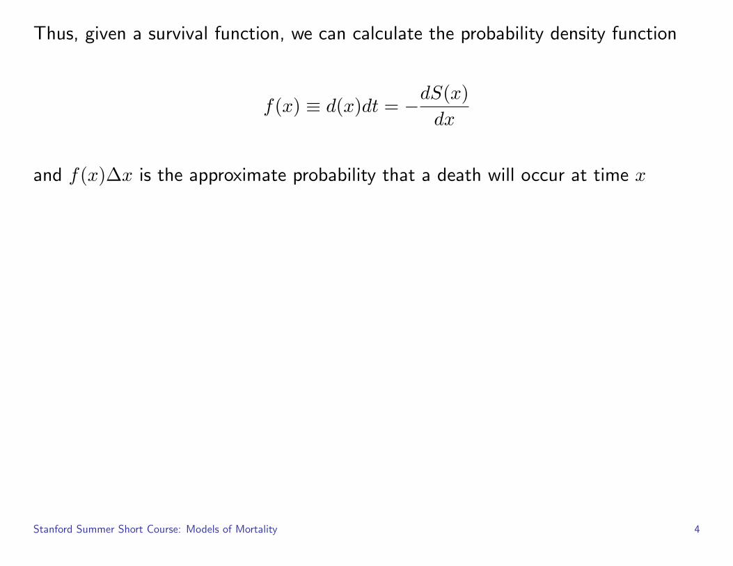
Thus, given a survival function, we can calculate the probability density function
f(x) ≡ d(x)dt = −dS(x)dx
and f(x)∆x is the approximate probability that a death will occur at time x
Stanford Summer Short Course: Models of Mortality 4
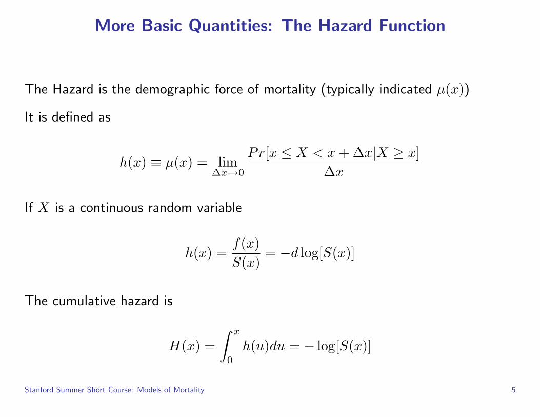
More Basic Quantities: The Hazard Function
The Hazard is the demographic force of mortality (typically indicated µ(x))
It is defined as
h(x) ≡ µ(x) = lim∆x→0
Pr[x ≤ X < x + ∆x|X ≥ x]∆x
If X is a continuous random variable
h(x) =f(x)S(x)
= −d log[S(x)]
The cumulative hazard is
H(x) =∫ x
0
h(u)du = − log[S(x)]
Stanford Summer Short Course: Models of Mortality 5
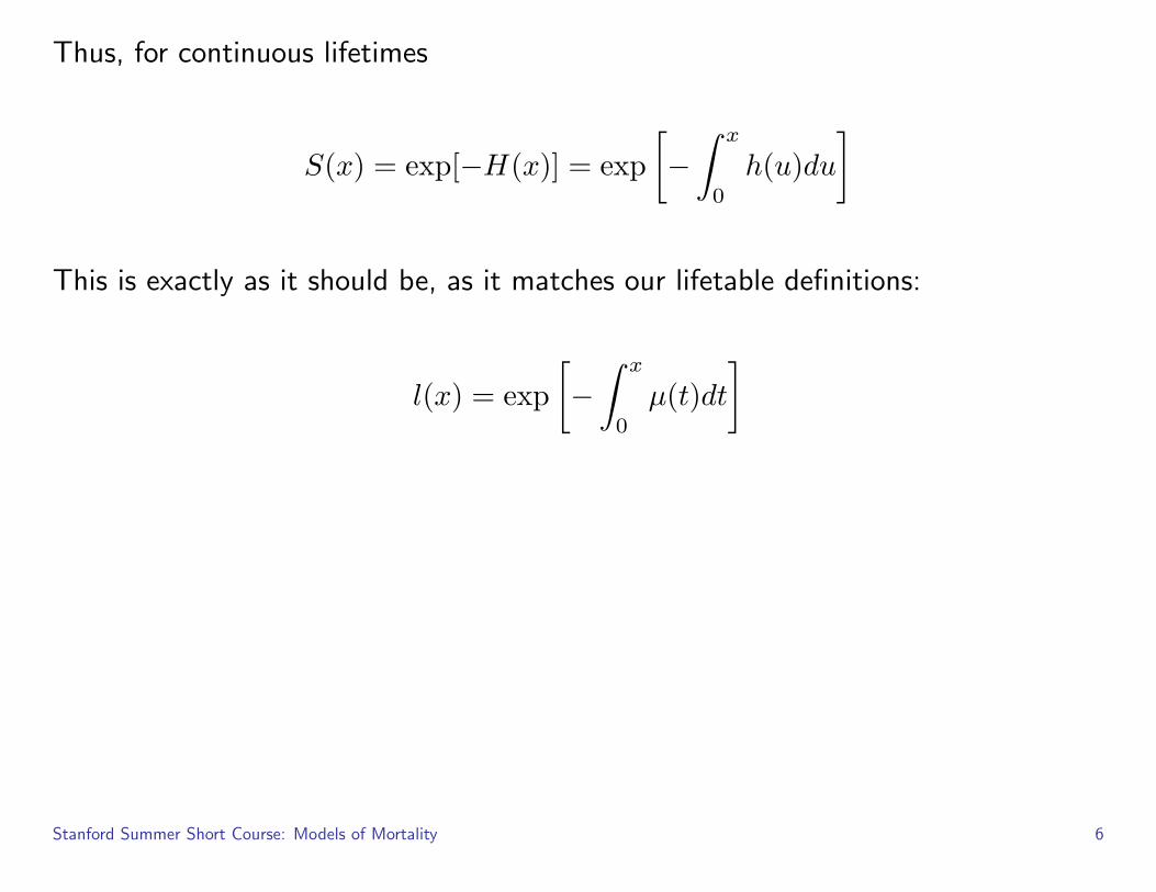
Thus, for continuous lifetimes
S(x) = exp[−H(x)] = exp[−
∫ x
0
h(u)du
]
This is exactly as it should be, as it matches our lifetable definitions:
l(x) = exp[−
∫ x
0
µ(t)dt
]
Stanford Summer Short Course: Models of Mortality 6
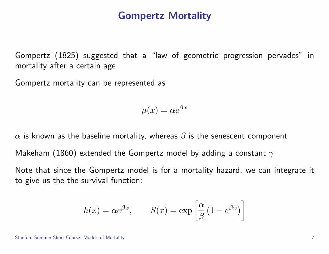
Gompertz Mortality
Gompertz (1825) suggested that a “law of geometric progression pervades” inmortality after a certain age
Gompertz mortality can be represented as
µ(x) = αeβx
α is known as the baseline mortality, whereas β is the senescent component
Makeham (1860) extended the Gompertz model by adding a constant γ
Note that since the Gompertz model is for a mortality hazard, we can integrate itto give us the the survival function:
h(x) = αeβx, S(x) = exp[α
β
(1− eβx
)]Stanford Summer Short Course: Models of Mortality 7
Also note that log-mortality is a linear function of age
log µ(x) = log(α) + βx
This suggests a regression approach my be useful
Stanford Summer Short Course: Models of Mortality 8
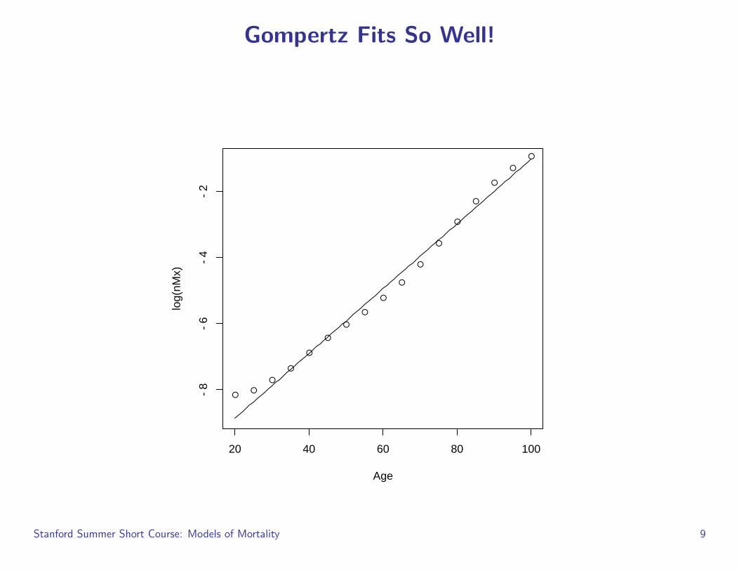
Gompertz Fits So Well!
20 40 60 80 100
−8
−6
−4
−2
Age
log(
nMx)
●●
●
●
●
●
●
●
●
●
●
●
●
●
●
●
●
Stanford Summer Short Course: Models of Mortality 9
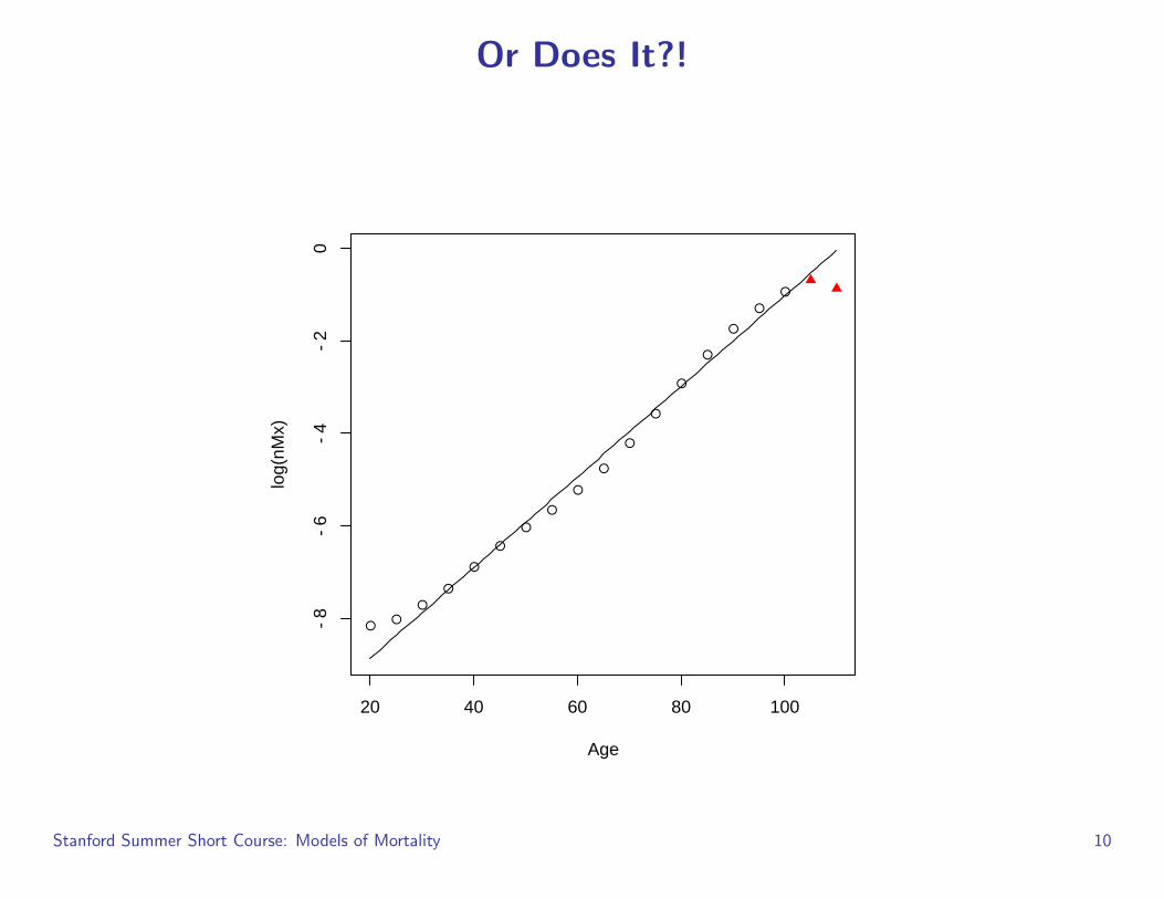
Or Does It?!
20 40 60 80 100
−8
−6
−4
−2
0
Age
log(
nMx)
●●
●
●
●
●
●
●
●
●
●
●
●
●
●
●
●
Stanford Summer Short Course: Models of Mortality 10
Other Mathematical Models of Mortality
Advantages:
• Compact, small number of parameters
• Highly interpretable
• Generalizable
• Good for comparative work (particularly interspecific comparisons)
Disadvantages:
• Hard to fit
• Numerical estimates frequently unstable (correlation between components)
• Almost certainly “wrong”
• What if there is a new source of mortality that is not covered by the model?
Stanford Summer Short Course: Models of Mortality 11
Two Models
Despite their shortcomings, two models are of interest:
1. Siler 5-Component Competing Hazard2. Heligman-Pollard 8-Component Model
Stanford Summer Short Course: Models of Mortality 12
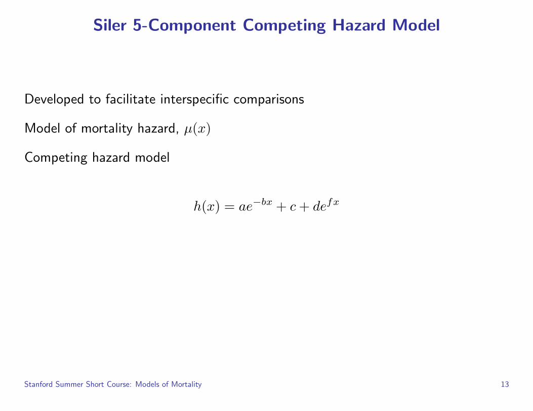
Siler 5-Component Competing Hazard Model
Developed to facilitate interspecific comparisons
Model of mortality hazard, µ(x)
Competing hazard model
h(x) = ae−bx + c + defx
Stanford Summer Short Course: Models of Mortality 13
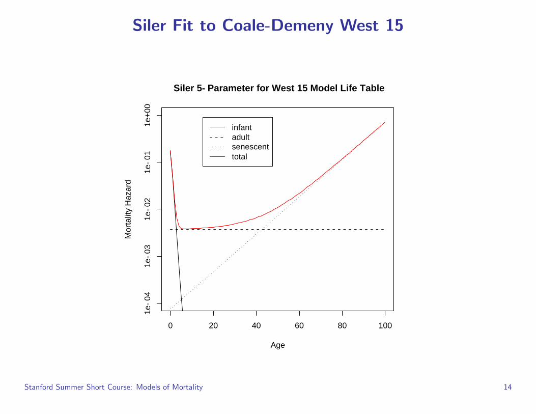
Siler Fit to Coale-Demeny West 15
0 20 40 60 80 100
1e−
041e
−03
1e−
021e
−01
1e+
00
Age
Mor
talit
y H
azar
dinfantadultsenescenttotal
Siler 5−Parameter for West 15 Model Life Table
Stanford Summer Short Course: Models of Mortality 14
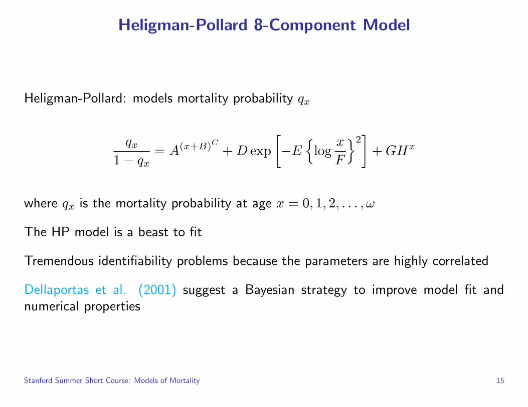
Heligman-Pollard 8-Component Model
Heligman-Pollard: models mortality probability qx
qx
1− qx= A(x+B)C
+ D exp[−E
{log
x
F
}2]
+ GHx
where qx is the mortality probability at age x = 0, 1, 2, . . . , ω
The HP model is a beast to fit
Tremendous identifiability problems because the parameters are highly correlated
Dellaportas et al. (2001) suggest a Bayesian strategy to improve model fit andnumerical properties
Stanford Summer Short Course: Models of Mortality 15
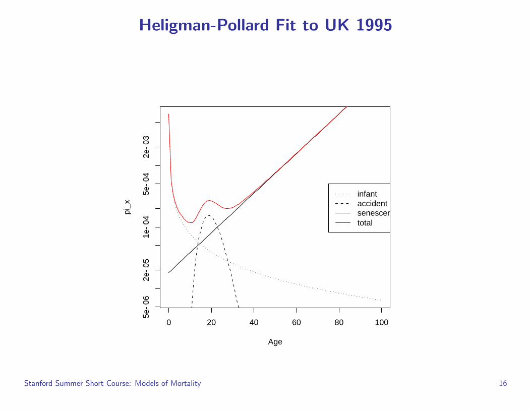
Heligman-Pollard Fit to UK 1995
0 20 40 60 80 100
5e−
062e
−05
1e−
045e
−04
2e−
03
Age
pi_x
infantaccidentsenescenttotal
Stanford Summer Short Course: Models of Mortality 16
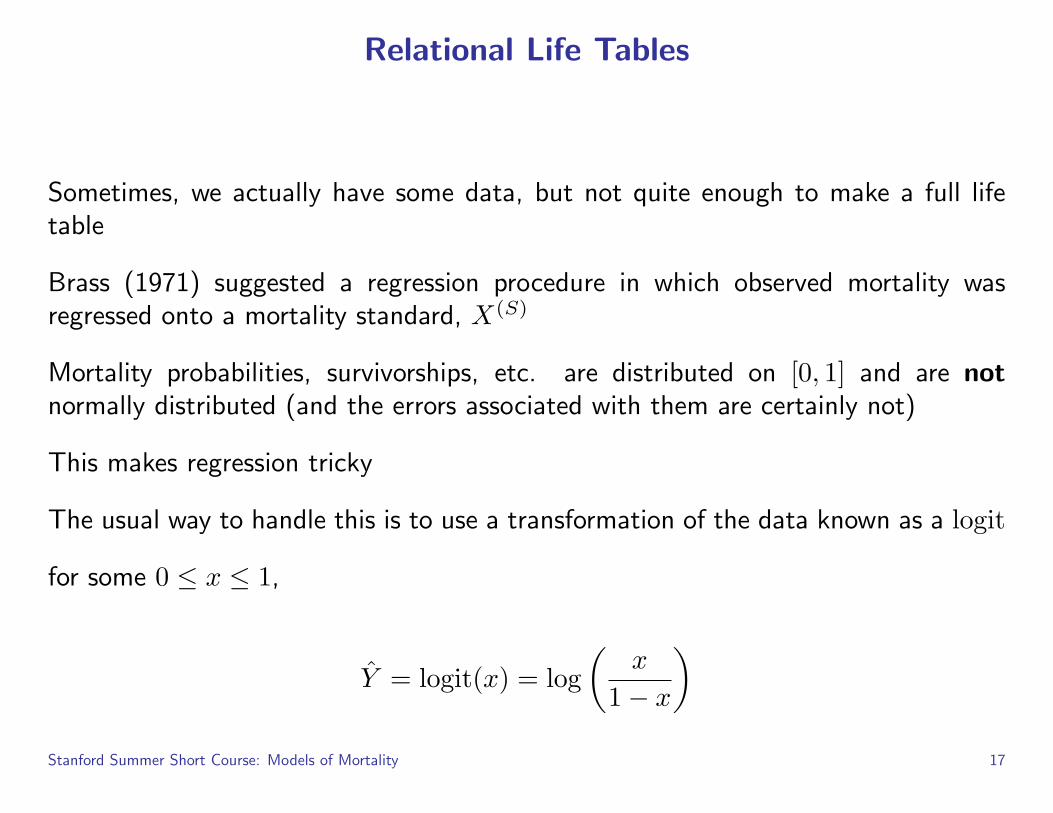
Relational Life Tables
Sometimes, we actually have some data, but not quite enough to make a full lifetable
Brass (1971) suggested a regression procedure in which observed mortality wasregressed onto a mortality standard, X(S)
Mortality probabilities, survivorships, etc. are distributed on [0, 1] and are notnormally distributed (and the errors associated with them are certainly not)
This makes regression tricky
The usual way to handle this is to use a transformation of the data known as a logit
for some 0 ≤ x ≤ 1,
Y = logit(x) = log(
x
1− x
)Stanford Summer Short Course: Models of Mortality 17
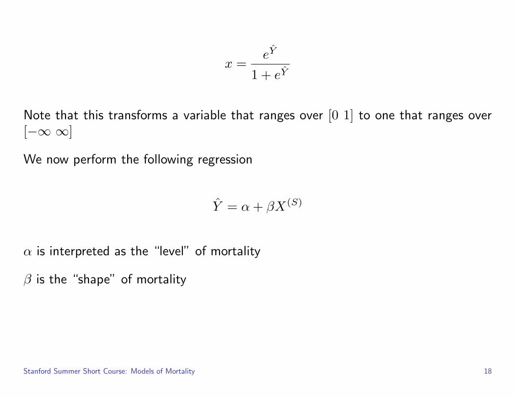
x =eY
1 + eY
Note that this transforms a variable that ranges over [0 1] to one that ranges over[−∞ ∞]
We now perform the following regression
Y = α + βX(S)
α is interpreted as the “level” of mortality
β is the “shape” of mortality
Stanford Summer Short Course: Models of Mortality 18
Be Careful! The notational usage in Preston et al. (2001) on this topic is notparticularly standard
. qx is not the standard 5-year mortality probability at age x
. qx is really 1− lx
. Perhaps a better notation would be xq0
Stanford Summer Short Course: Models of Mortality 19
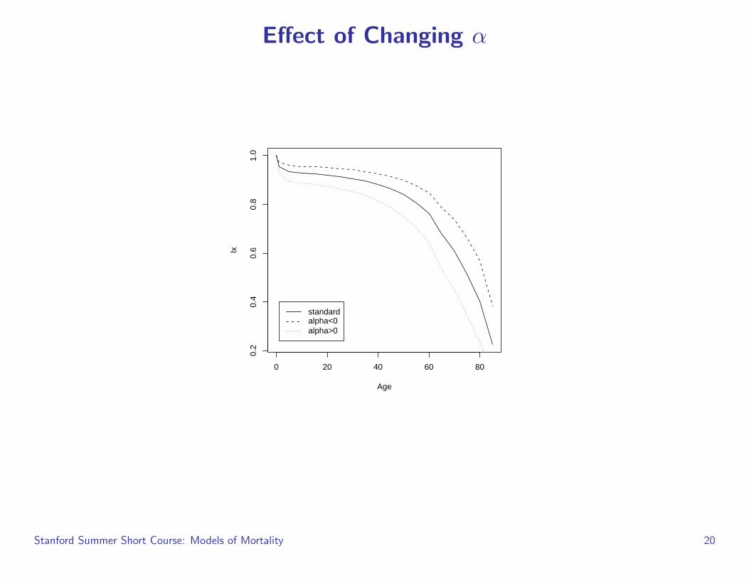
Effect of Changing α
0 20 40 60 80
0.2
0.4
0.6
0.8
1.0
Age
lx
standardalpha<0alpha>0
Stanford Summer Short Course: Models of Mortality 20
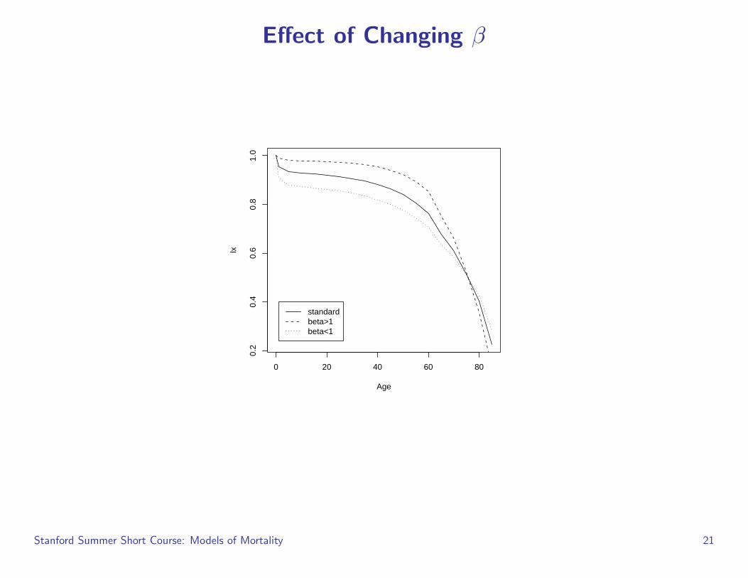
Effect of Changing β
0 20 40 60 80
0.2
0.4
0.6
0.8
1.0
Age
lx
standardbeta>1beta<1
Stanford Summer Short Course: Models of Mortality 21

Model Life Tables
There are a variety of model life table systems
1. UN (1958, 1982)2. Coale & Demeny (1966, 1983)3. INDEPTH4. Weiss, 1973 (Obscure anthropological model life tables)
Stanford Summer Short Course: Models of Mortality 22

Model Life Table Construction
Model life table construction involves three general steps
• Gather a lot of high quality life tables
• Use Multivariate Analysis Techniques (e.g., PCA) to find clusters
• Combine them to provide a standard
Stanford Summer Short Course: Models of Mortality 23
Coale-Demeny Regional Model Life Tables
The Coale & Demeny is broken down into 4 “Regional” Models: North, South,East, and West
North Sweden pre-1920, Norway, Iceland: low infant and post-50 mortalitySouth Spain, Portugal, Southern Italy: high infant and post-65 mortalityEast Austria, Germany, Northern Italy, Hungary, Poland: mortality rates generally
high, particularly after 50West Everything else: Most frequent anthropological application
They are indexed (typically) by life expectancy at birth or age 10
Use of model life tables follows a simple recipe:
1. Use whatever information available to estimate life expectancy2. Use whatever information available to determine the mortality pattern (or use
West model life table)3. Use the table that fits your assumptions
Stanford Summer Short Course: Models of Mortality 24
Model Life Tables Construction
Component mortality models (e.g., Coale-Demeny)
m = Ca
where m is a vector of logit(nqx) values for x ∈ 0 . . . k
C is a k× l +1 matrix of loadings of the k ages on the first l components of a PCA(with a leading column of ones)
a is an l + 1× 1 vector of coefficients
a estimated by regressing empirically-derived values of logit(nqx) on C
Stanford Summer Short Course: Models of Mortality 25
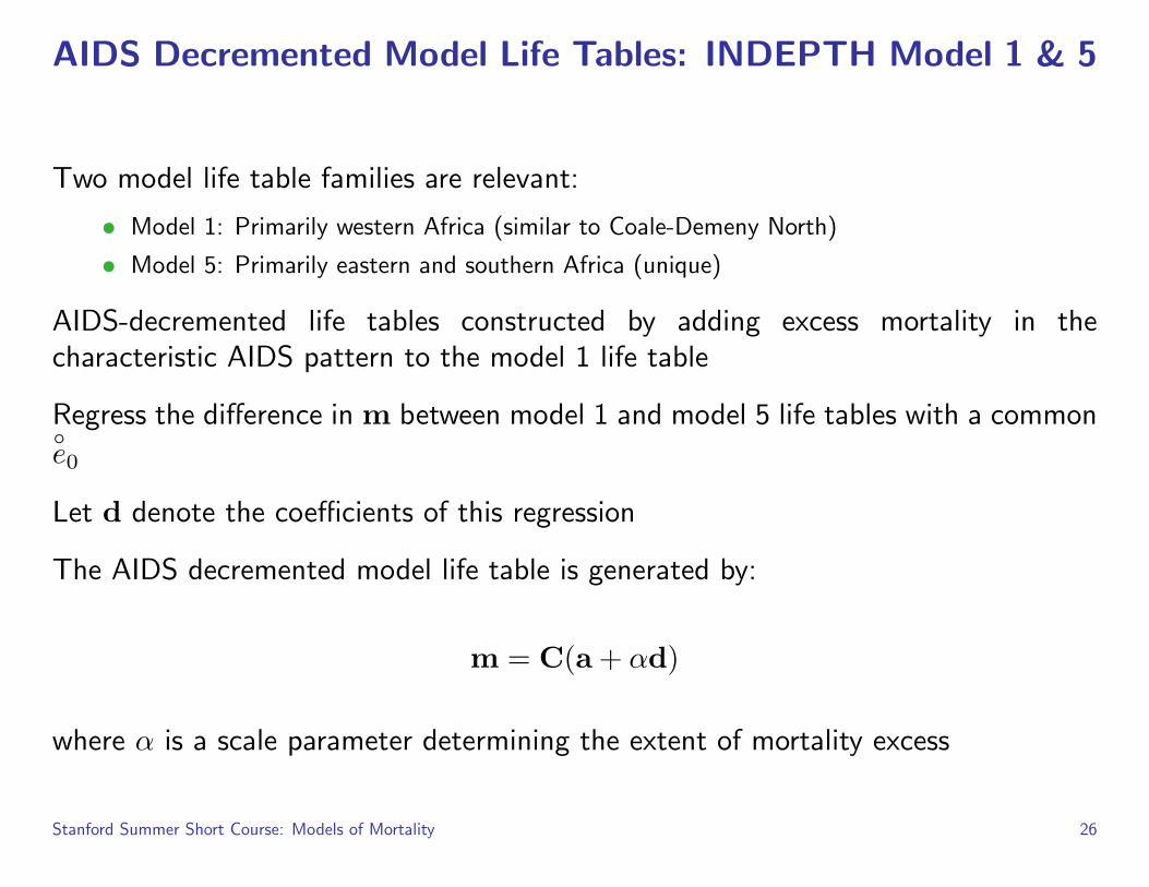
AIDS Decremented Model Life Tables: INDEPTH Model 1 & 5
Two model life table families are relevant:
• Model 1: Primarily western Africa (similar to Coale-Demeny North)
• Model 5: Primarily eastern and southern Africa (unique)
AIDS-decremented life tables constructed by adding excess mortality in thecharacteristic AIDS pattern to the model 1 life table
Regress the difference in m between model 1 and model 5 life tables with a common◦e0
Let d denote the coefficients of this regression
The AIDS decremented model life table is generated by:
m = C(a + αd)
where α is a scale parameter determining the extent of mortality excess
Stanford Summer Short Course: Models of Mortality 26
INDEPTH AIDS-Decremented Model Life Tables
0 20 40 60 80
0.2
0.4
0.6
0.8
1.0
Age
Sur
vivo
rshi
p
0 20 40 60 80
0.2
0.4
0.6
0.8
1.0
Age
Sur
vivo
rshi
p
Stanford Summer Short Course: Models of Mortality 27
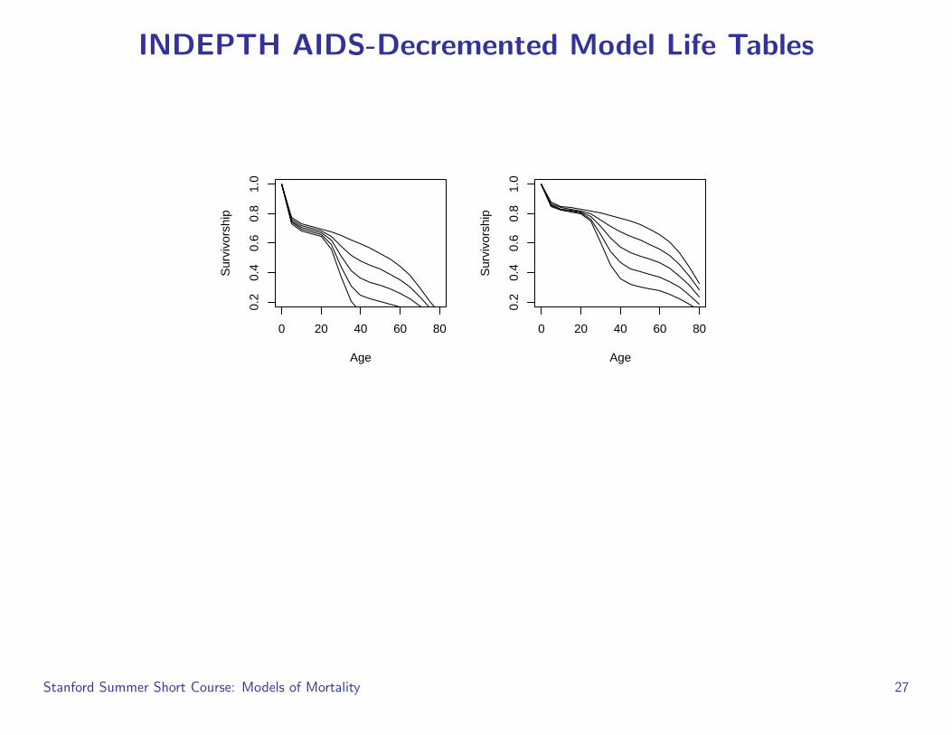
AIDS Creates More Orphans
0 5 10 15
0.0
0.1
0.2
0.3
0.4
Age
Con
ditio
nal P
roba
bilit
y of
Orp
hanh
ood
Stanford Summer Short Course: Models of Mortality 28
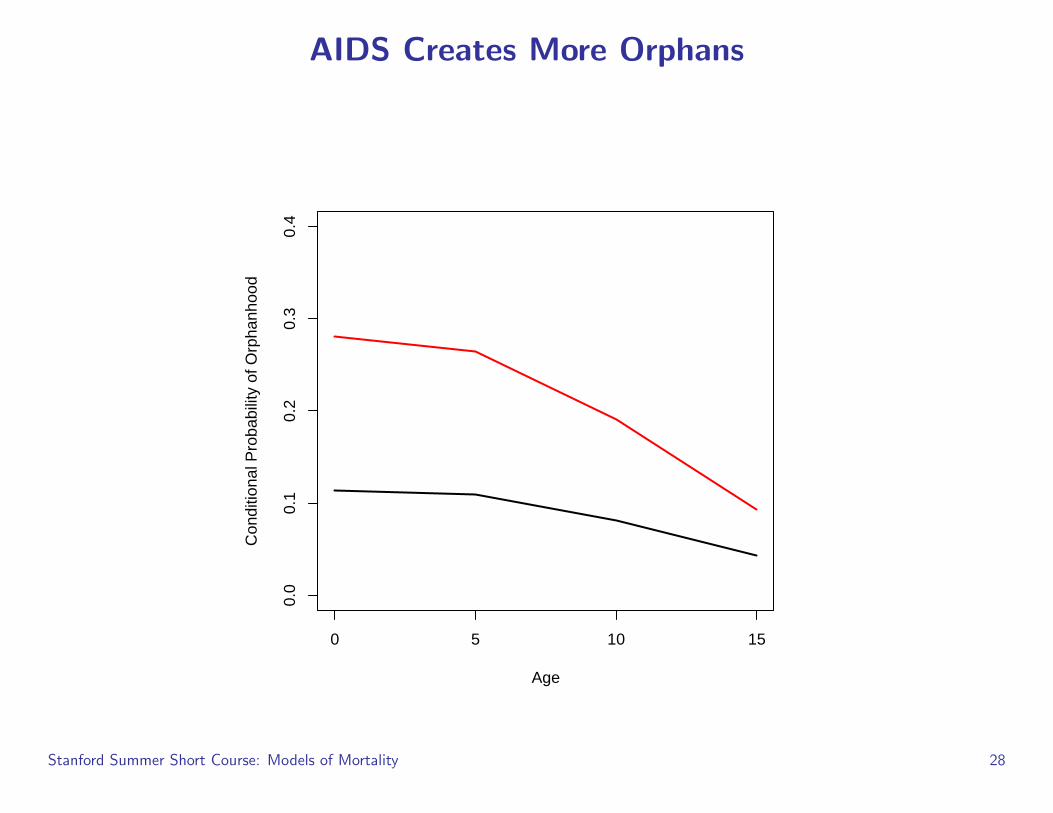
It’s the Pattern of Mortality that Matters
0 5 10 15
0.0
0.2
0.4
Age
Pr(
Orp
han)
5 Year Decrement
0 5 10 15
0.0
0.2
0.4
Age
Pr(
Orp
han)
10 Year Decrement
0 5 10 15
0.0
0.2
0.4
Age
Pr(
Orp
han)
15 Year Decrement
0 5 10 15
0.0
0.2
0.4
Age
Pr(
Orp
han)
20 Year Decrement
Stanford Summer Short Course: Models of Mortality 29
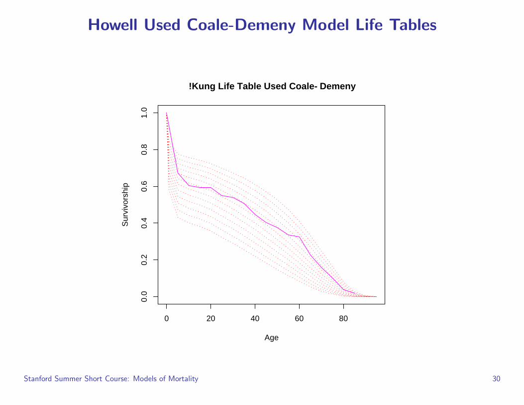
Howell Used Coale-Demeny Model Life Tables
0 20 40 60 80
0.0
0.2
0.4
0.6
0.8
1.0
Age
Sur
vivo
rshi
p
!Kung Life Table Used Coale−Demeny
Stanford Summer Short Course: Models of Mortality 30
Hill & Hurtado Did Not
0 20 40 60 80
0.0
0.2
0.4
0.6
0.8
1.0
Age
Sur
vivo
rshi
p
Ache Life Table Did Not Use Coale−Demeny
Ache!Kung
Stanford Summer Short Course: Models of Mortality 31
0 20 40 60 80
0.0
0.2
0.4
0.6
0.8
1.0
Age
Sur
vivo
rshi
p
Ache!KungYanomamoGombe
Stanford Summer Short Course: Models of Mortality 32
0 20 40 60 80
0.0
0.4
0.8
Age
Sur
vivo
rshi
p
15 20 25 30 35 40 45
0.0
0.4
0.8
1.2
Age
AS
FR
0.2 0.4 0.6 0.8 1.0
0.05
0.10
0.15
Relative Age
dx
Proportion in the Chimp Life Table
Pro
port
ion
in H
uman
Life
Tab
le
0.5
1.5
2.5
0.0 0.2 0.4 0.6 0.8 1.0
Stanford Summer Short Course: Models of Mortality 33
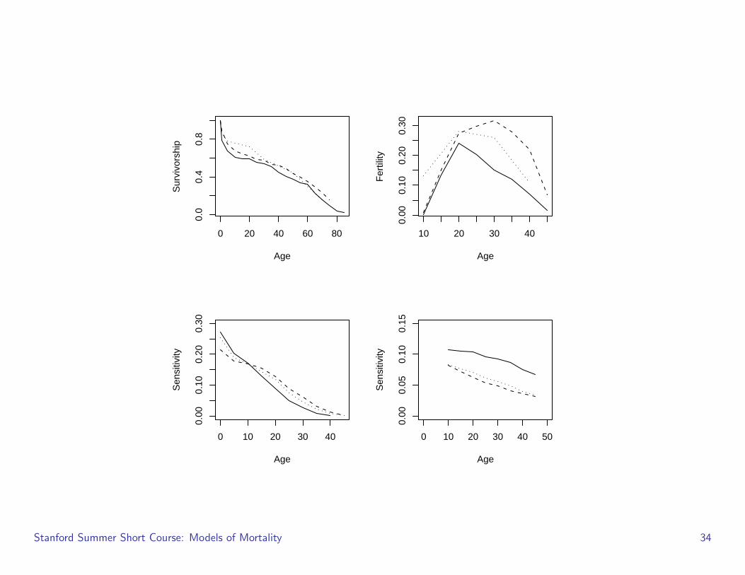
0 20 40 60 80
0.0
0.4
0.8
Age
Sur
vivo
rshi
p
10 20 30 40
0.00
0.10
0.20
0.30
Age
Fer
tility
0 10 20 30 40
0.00
0.10
0.20
0.30
Age
Sen
sitiv
ity
0 10 20 30 40 50
0.00
0.05
0.10
0.15
Age
Sen
sitiv
ity
Stanford Summer Short Course: Models of Mortality 34