Embed Size (px)
Citation preview

MATHEMATICAL APPENDIX to
Optimal continuous cover forest management:- Economic and environmental effects and legal considerations
Professor Dr Peter Lohmander http://www.Lohmander.com
BIT's 5th Low Carbon Earth Summit (LCES 2015 & ICE-2015)
Theme: "Take Actions for Rebuilding a Clean World"
September 24-26, 2015
Venue: Xi'an, China
1

This mathematical appendix includes derivations of most of the results presented in:
”Optimal continuous cover forest management:- Economic and environmental effects and legal considerations”
by
Professor Dr Peter Lohmanderhttp://www.Lohmander.com
BIT's 5th Low Carbon Earth Summit (LCES 2015 & ICE-2015)
Theme: "Take Actions for Rebuilding a Clean World"September 24-26, 2015
Venue: Xi'an, China
2

3
Lohmander 150824 China File
One and two dimensional optimization and comparative statistics in the
volume and time interval dimensions
Peter Lohmander 2015-08-24
One dimensional optimization and comparative statistics in the time interval dimension
General Problem Definition
1 1( , ) ( , )max ( )
1rt
P v t Q v t cR h
e
0 1
. .s t
h v v
Obs: Generalized P(.), Q(.) and R(.). Assumption: r > 0.

4
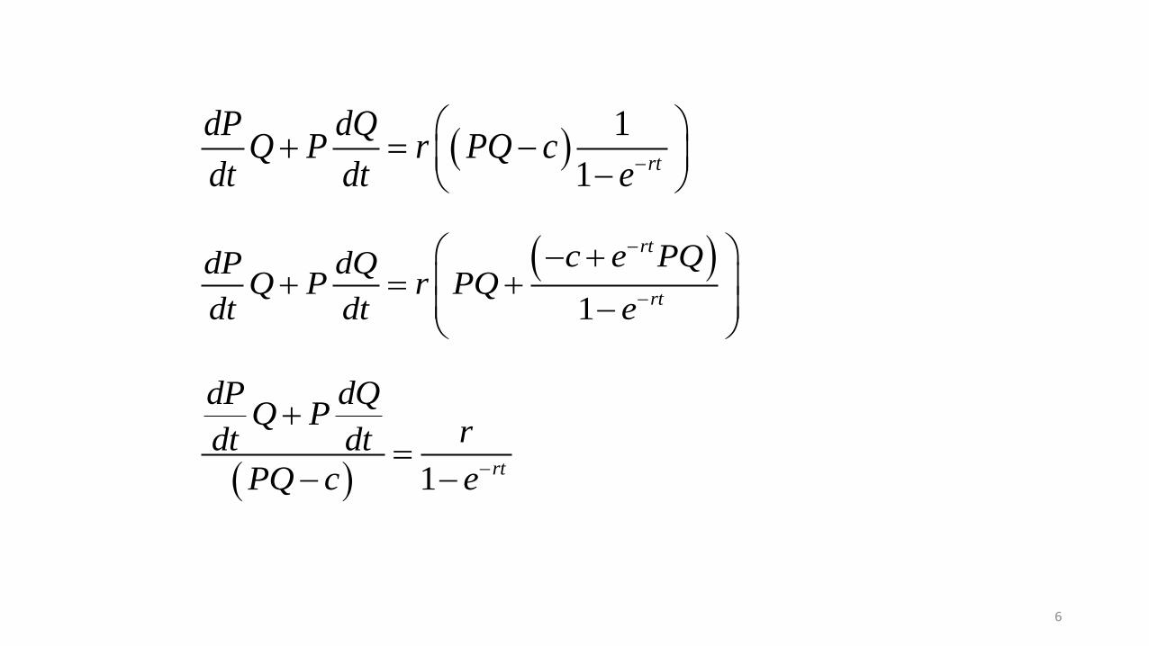
Derivation of optimal General Principles
2
11 0
1
rt rt
rt
d dP dQQ P e PQ c re
dt dt dte
21 0
1
rtrt
rt
d e dP dQQ P e PQ c r
dt dt dte
2
(.) 01
rt
rt
ek
e
(.) 1 0rtdP dQM Q P e PQ c r
dt dt
(.) 0M

5
(.) 0M
Optimal principles in the time dimension that can be given economic interpretations:
1
1 rt
dP dQQ P
dt dt r
PQ ce
1
rt
rt
dP dQQ P
dt dt rc e PQ
PQe
6
1
1 rt
dP dQQ P r PQ c
dt dt e
1
rt
rt
c e PQdP dQQ P r PQ
dt dt e
1 rt
dP dQQ P
rdt dt
PQ c e

7
Comparative statistics analyses based on one dimensional optimization:
How is the optimal time interval affected if the parameter c marginally increases (ceteres paribus)?
The time intervals are optimized:
0d
dt
If parameter changes take place, we still want the time interval to be optimal:
0d
ddt

8
2 2*
20
d d dd dt dc
dt dt dtdc
2 2*
2
d ddt dc
dt dtdc
2
*
2
2
d
dtdcdt
dc d
dt
A unique optimum is assumed in the time interval dimension. As a consequence:
2
20
d
dt

9
2
(.) 0d
k rdtdc
2
*
2
2
0
d
dtdcdt
dc d
dt
Conclusion:
The optimal time interval is a strictly increasing function of the parameter c.

10
Comparative statistics analyses based on one dimensional optimization:
How is the optimal time interval affected if the parameter r marginally increases (ceteres paribus)?
The time intervals are optimized:
0d
dt
If parameter changes take place, we still want the time interval to be optimal:
0d
ddt

11
2 2*
20
d d dd dt dr
dt dt dtdr
2 2*
2
d ddt dr
dt dtdr
2
*
2
2
d
dtdrdt
dr d
dt
A unique optimum is assumed in the time interval dimension. As a consequence:
2
20
d
dt

12
2
?d
dtdr
2d dk dMM k
dtdr dr dr
2
0 0d d dM
M kdt dtdr dr
2
0 sgn sgnd dM
kdtdr dr

13
(.) 1 0rtdP dQM Q P e PQ c r
dt dt
rtdM dP dQQ P te PQ c
dr dt dt
rtdM dP dQr Q P rte PQ c r
dr dt dt
1rt rtdM dP dQr M Q P rte e
dr dt dt

14
_
0dP dQ
w Q Pdt dt
1rt rtw rte e
_
sgn 0 sgn sgndM
r ww wdr

15
The usual case:
2
0 sgn sgn sgnd dM
r wdtdr dr
1rt rtw rte e
x rt
1x xw xe e
( ) 1 1xw x x e

16
(0) 0w
1 1x xdwe x e
dx
xdwxe
dx
0
0x
dw
dx
0
0x
dw
dx

17
0x rt
0( ) 0
xw x
2
sgn sgn 0d
wdtdr

18
The unusual case:
2
0 sgn sgn sgnd dM
r wdtdr dr
0x rt
0( ) 0
xw x
2
sgn sgn 0d
wdtdr

19
In both cases:
2
0d
dtdr
2
*
2
2
0
d
dtdrdt
dr d
dt
Conclusion:
The optimal time interval is a strictly decreasing function of the parameter r.

20
Comparative statistics analyses based on one dimensional optimization:
How is the optimal time interval affected if the future prices marginally increase (ceteres paribus)?
In order to study the effects of prices on the optimal time interval, useful parameters are needed.
The problem is originally:
1 1( , ) ( , )max ( )
1rt
P v t Q v t cR h
e
Here, we replace this problem by this problem:
1( , )max ( )
1rt
pQ v t cR h
e

21
How is the optimal time interval affected if the parameter p marginally increases (ceteres paribus)?
The time intervals are optimized:
0d
dt
If parameter changes take place, we still want the time interval to be optimal:
0d
ddt

22
2 2*
20
d d dd dt dp
dt dt dtdp
2 2*
2
d ddt dp
dt dtdp
2
*
2
2
d
dtdpdt
dp d
dt

23
A unique optimum is assumed in the time interval dimension. As a consequence:
2
20
d
dt
2
11 0
1
rt rt
rt
d dQp e pQ c re
dt dte
21 0
1
rtrt
rt
d e dQp e pQ c r
dt dte

24
2
(.) 01
rt
rt
ek
e
1(.) 1 0rtdQM p e pQ c r
dt
2
(.) 1 rtd dQk e Q r
dtdp dt
2
(.) 1 rtd dQp k p e pQ r
dtdp dt

25
2
(.)d d
p k crdtdp dt
2
( 0) ( 0) 0 0d d
p crdt dtdp
2
*
2
2
0
d
dtdpdt
dp d
dt
Conclusion:
The optimal time interval is a strictly decreasing function of the parameter p.

26
One dimensional optimization and comparative statistics in the volume dimension
General Problem Definition
1 1( , ) ( , )max ( )
1rt
P v t Q v t cR h
e
0 1
. .s t
h v v
Obs: Generalized P(.), Q(.) and R(.). t > 0. Assumption: r > 0.

27
1 1 1 1
1(.) 0
1rt
d dR dh dP dQQ P
dv dh dv e dv dv
1
1dh
dv
The first order optimum condition implies:
1 1
1(.)
1rt
dR dP dQQ P
dh e dv dv
28
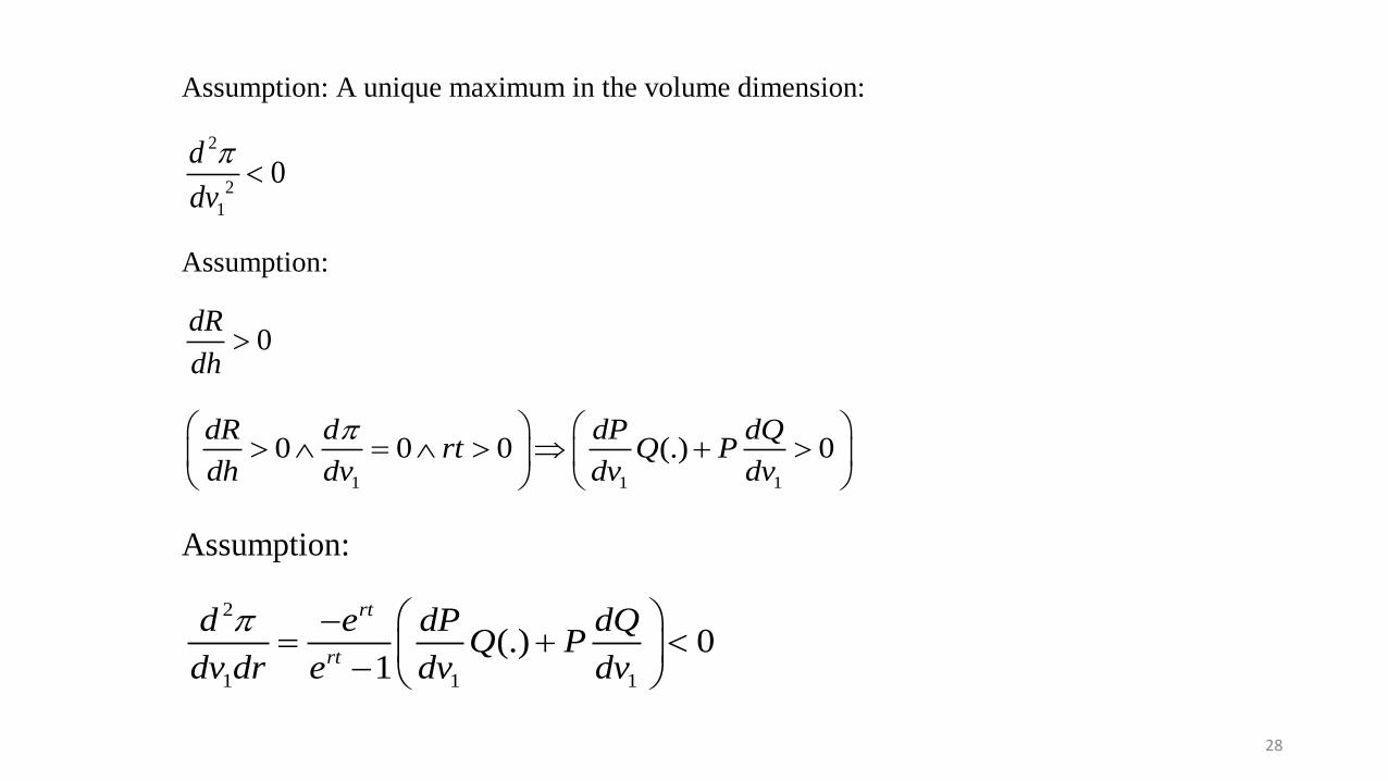
Assumption: A unique maximum in the volume dimension:
2
2
1
0d
dv
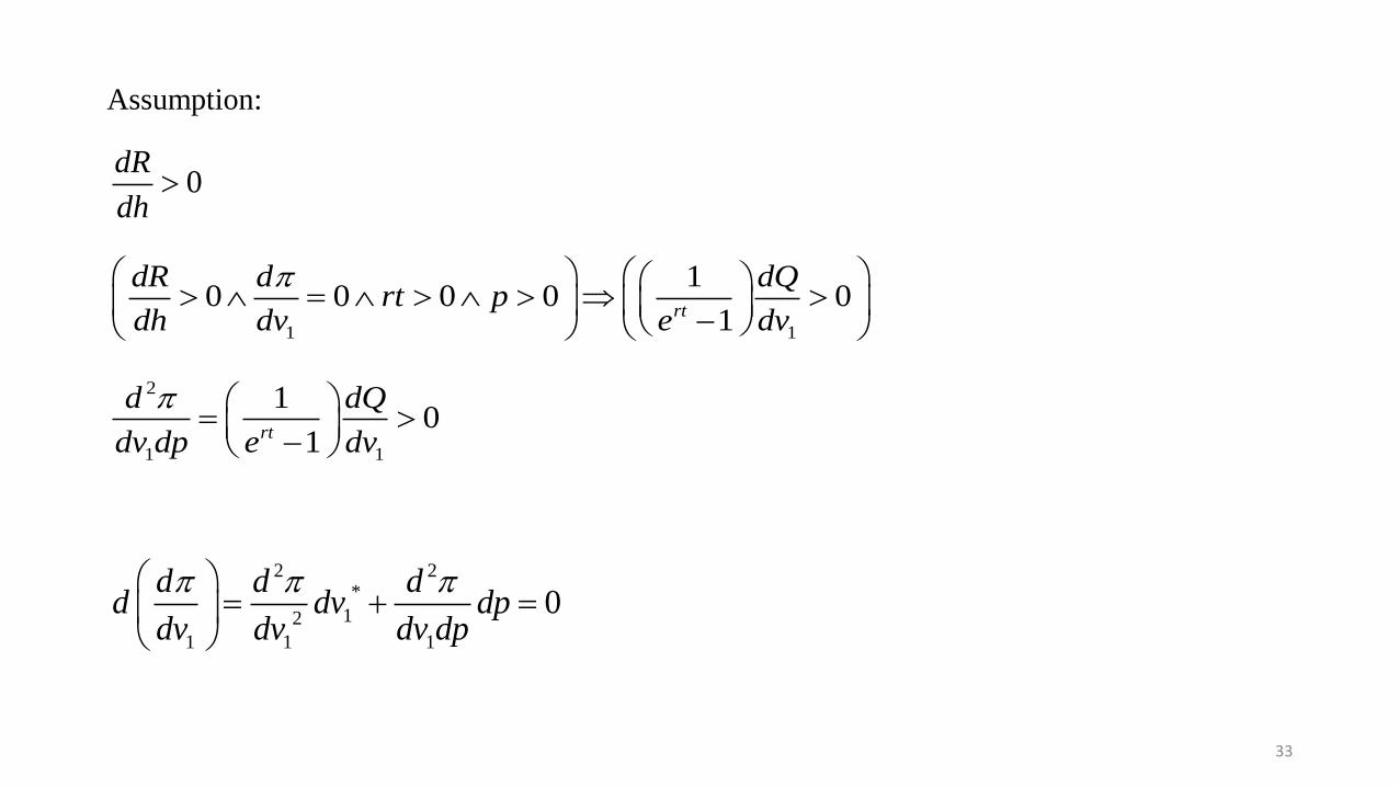
Assumption:
0dR
dh
1 1 1
0 0 0 (.) 0dR d dP dQ
rt Q Pdh dv dv dv
Assumption:
2
1 1 1
(.) 01
rt
rt
d e dP dQQ P
dv dr e dv dv
29
Comparative statistics analyses based on one dimensional optimization:
How is the optimal volume affected if the parameter r marginally increases (ceteres paribus)?
The volume is optimized:
1
0d
dv
If parameter changes take place, we still want the volume to be optimal:
1
0d
ddv

30
2 2*
12
1 1 1
0d d d
d dv drdv dv dv dr
2 2*
12
1 1
0d d
dv drdv dv dr
2 2
*
12
1 1
d ddv dr
dv dv dr
2
*11
2
2
1
0
d
dv drdv
dr d
dv
Conclusion:
The optimal volume is a strictly decreasing function of the parameter r.

31
Comparative statistics analyses based on one dimensional optimization:
How is the optimal volume affected if the future prices marginally increase (ceteres paribus)?
In order to study the effects of prices on the optimal time interval, useful parameters are needed.
The problem is originally:
1 1( , ) ( , )max ( )
1rt
P v t Q v t cR h
e
Here, we replace this problem by this problem:
1( , )max ( )
1rt
pQ v t cR h
e

32
1 1 1
10
1rt
d dR dh dQp
dv dh dv e dv
2
1 1
1
1rt
d dQ
dv dp e dv
The first order optimum condition implies:
1
1
1rt
dR dQp
dh e dv
Assumption: A unique maximum in the volume dimension:
2
2
1
0d
dv
33
Assumption:
0dR
dh
1 1
10 0 0 0 0
1rt
dR d dQrt p
dh dv e dv
2
1 1
10
1rt
d dQ
dv dp e dv
2 2*
12
1 1 1
0d d d
d dv dpdv dv dv dp

34
2 2*
12
1 1
0d d
dv dpdv dv dp
2 2
*
12
1 1
d ddv dp
dv dv dp
2
*11
2
2
1
0
d
dv dpdv
dp d
dv
Conclusion:
The optimal volume is a strictly increasing function of the parameter p.
35
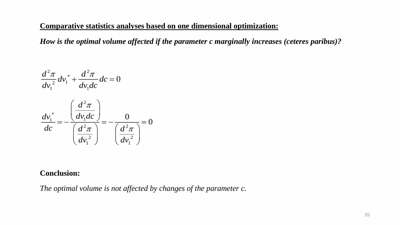
Comparative statistics analyses based on one dimensional optimization:
How is the optimal volume affected if the parameter c marginally increases (ceteres paribus)?
2 2*
12
1 1
0d d
dv dcdv dv dc
2
*11
2 2
2 2
1 1
00
d
dv dcdv
dc d d
dv dv
Conclusion:
The optimal volume is not affected by changes of the parameter c.

36
Observation:
If the volume is constrained (by law or something else), we may study the effects of the volume
constraint on the optimal time interval, via one dimensional optimization and
comparative statics using 2
1
d
dv dt
.
Also, since 2 2
1 1
d d
dv dt dtdv
, we may perform the corresponding analysis of optimal volume based on
constrained t.
In both cases, it is necessary to know somehing about 2
1
d
dv dt
.
Below, we will also use 2
1
d
dv dt
in another way, in two dimensional optimization of the time interval
and the volume.

37
We will soon discover that 2
1
0d
dv dt
.
In ”one dimensional optimization” and comparative statics analysis, we come to the following
conclusions:
2
*1
21
2
0
d
dtdvdt
dv d
dt
and
2
*11
2
2
1
0
d
dv dtdv
dt d
dv
38
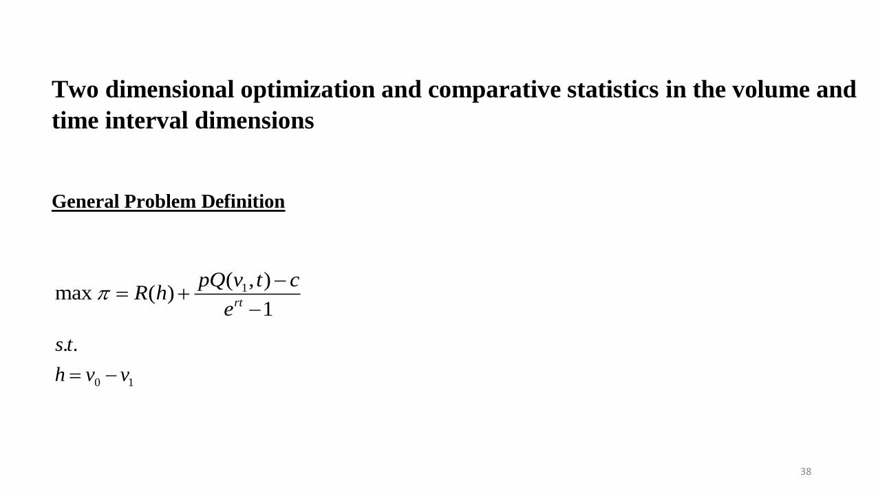
Two dimensional optimization and comparative statistics in the volume and
time interval dimensions
General Problem Definition
1( , )max ( )
1rt
pQ v t cR h
e
0 1
. .s t
h v v

39
The first order optimum conditions:
1
0
0
d
dv
d
dt
1 1
2
10
1
1 01
rt
rtrt
rt
dR dh dQp
dh dv e dv
e dQp e pQ c r
dte

40
Assumption: A unique maximum exists. The following conditions hold:
2 2
22 21 1
2 2 2 21
2
1
0, 0, 0
d d
dv dv dtd d
dv dt d d
dtdv dt
For a unique maximum, it is sufficient that:
2 2
221 1
2 2 21
2
1
0, 0
d d
dv dv dtd
dv d d
dtdv dt

41
In the analysis, it will turn out that it is important to know something about
2 2
1 1
d d
dv dt dtdv
, at least the sign.
2 2
2 2 2 2 21 1
2 22 21 1 1
2
1
0 0
d d
dv dv dt d d d dD
dv dt dtdv dv dtd d
dtdv dt

42
22 2 2 2 2
2 2
1 1 1 1
d d d d d
dv dt dtdv dv dt dv dt
Observation:
22
1
d
dv dt
is usually small in relation to 2 2
2 2
1
d d
dv dt
.
2
1
d
dv dt
is however a function of several parameters
and decision variables, which makes it complicated to give general and explicit functions describing
the signs and absolute values of 2
1
d
dv dt
. In any case, the sign of
2
1
d
dv dt
will be determined.

43
Determination of the sign of 2
1
d
dv dt
:
1 1
10
1rt
d dR dQp
dv dh e dv
2 2
2
1 1 1
1
11
rt
rtrt
d re dQ d Qp p
dv dt dv e dv dte

44
2 2
1 1 11 1rt rt
d p d Q r dQ
dv dt e dtdv e dv
2
11 0
1
rt rt
rt
d dQp e pQ c re
dt dte
2 2
1 1 11 1rt rt
d p d Q r dQ
dtdv e dtdv e dv

45
Observation:
2 2 2
1 1 1 11 1rt rt
d d p d Q r dQ
dv dt dtdv e dtdv e dv
2
1
sgn sgnd
dv dt
2
1 11 rt
d Q r dQ
dv dt e dv

46
With relevant growth functions:
2 2
1 10
td Q d Q
ds tdv dt dv dt
2
1 10
td Q dQ
dsdv dt dv
2
1 1
d Q dQt
dv dt dv
21
1
, 0
dQ
dvd Qk k
dv dt t

47
2
1 11 rt
d Q r dQ
dv dt e dv
1
11 rt
dQ
dv r dQk
t e dv
1
1
1 rt
dQ rk
dv t e
Observation:
1
10 sgn sgn
1 rt
dQ rk
dv t e

48
Let 1 rt
rw
e
W(r=0) = ? Observation: Division by zero is not allowed.
0
1 1lim
1 1rt rtrtr
dr
r dr
e te td e
dr
01 1
1 1lim 0r
dQ dQk k
dv t t dv

49
1
1
1 rt
dQ rk
dv t e
2
1
1(1 )
1
rt rt
rt
e r ted dQ
dr dv e
2
1
11
1
rt rt
rt
d dQe rte
dr dv e

50
Let
1 (1 )rte rt
Observation:
sgn sgnd
dr
( 0) 0r
(1 )rt rtdte rt e t
dr
2 rtdrt e
dr

51
0 0 0d
r tdr
0 0 0r t
sgn sgnd
dr
0d
dr

52
0
lim 0 0 0r
d
dr
2
1
sgn sgnd
dv dt
2
1
0d
dv dt

53
Comparative statics analysis based on two dimensional optimization:
2 2 2 2 2
2 *1 1 1 1 11
*2 2 2 2 2
2
1
d d d d ddc dp dr
dv dv dt dv dc dv dp dv drdv
dtd d d d ddc dp dr
dtdv dt dtdc dtdp dtdr

54
First, we study the effects of changes in c , when 0dp dr .
2
1
0d
dv dc
2
20
1
rt
rt
d re
dtdc e

55
2 2 2
2 *1 1 1 1
*2 2 2
2
1
d d ddc
dv dv dt dv dv dc
dtd d ddc
dtdv dt dtdc
2 2 2 2
1 1 1 1
2 2 2 2
* 2 21
2 2
2
1 1
2 2
2
1
d d d d
dv dc dv dt dv dc dv dt
d d d d
dv dtdc dt dtdc dt
dc Dd d
dv dv dt
d d
dtdv dt

56
2
1
2 22 2
* 21 1
0d
dv dt
d dd d
dv dtdc dv dtdtdc dt
dc D D
*2 2
1
1
0 0 sgn sgndvd d
Ddtdc dc dv dt
Observation:
2
1
0d
dv dt
. As a consequence,
*
1 0dv
dc .

57
2 2 2
2 2
1 1 1
2 2 2 2 2 2
2*1 1 1
2 2
2
1 1
2 2
2
1
0
0
d d d
dv dv dc dv
d d d d d d
dtdv dtdc dtdv dtdc dv dtdcdt
dc D Dd d
dv dv dt
d d
dtdv dt

58
Second, we study the effects of changes in p , when 0dc dr .
2
1 1
10
1rt
d dQ
dv dp e dv
2
2
11
1
rt rt
rt
d dQe Q re
dtdp dte
2
2
11
1
rt rt
rt
d dQp p e pQ re
dtdp dte

59
2
2
10
1
rt
rt
d dp cre
dtdp dt e
2
0 0 0d d
pdt dtdp
2 2 2
2 *1 1 11
*2 2 2
2
1
d d ddp
dv dv dt dv dpdv
dtd d ddp
dtdv dt dtdp

60
2 2 2 2
1 1 1 1
2 2 2 2
2 2*
1
2 2
2
1 1
2 2
2
1
d d d d
dv dp dv dt dv dp dv dt
d d d d
dtdp dt dtdp dtdv
dp Dd d
dv dv dt
d d
dtdv dt
2 2
1 1
2 2 2 2 2 2
2* 2
1 1 1 0
d d
dv dp dv dt
d d d d d d
dtdp dtdv dv dp dt dtdp dv dt
dp D D

61
2 2
2
1 1
2 2 2 2 2 2
2*1 1 1 1 0
d d
dv dv dp
d d d d d d
dtdv dtdp dv dtdp dtdv dv dpdt
dp D D
62
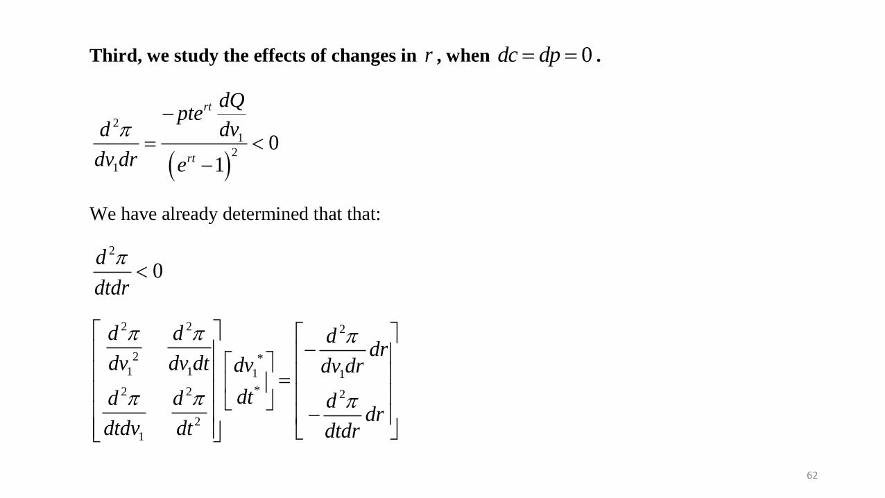
Third, we study the effects of changes in r , when 0dc dp .
2
1
2
1
01
rt
rt
dQpte
dvd
dv dr e
We have already determined that that:
2
0d
dtdr
2 2 2
2 *1 1 1 1
*2 2 2
2
1
d d ddr
dv dv dt dv dv dr
dtd d ddr
dtdv dt dtdr

63
2 2 2 2
1 1 1 1
2 2 2 2
* 2 21
2 2
2
1 1
2 2
2
1
d d d d
dv dr dv dt dv dr dv dt
d d d d
dv dtdr dt dtdr dt
dr Dd d
dv dv dt
d d
dtdv dt
2 2
1 1
2 2 2 22 2
* 221 1 1
d d
dv dr dv dt
d d d dd d
dv dv dr dt dtdr dv dtdtdr dt
dr D D
2
1
d
dv dt
is negative but has a low absolute value. As a result:
*
1 0dv
dr

64
2 2
2
1 1
2 2 2 2 2 2
2*1 1 1 1
2 2
2
1 1
2 2
2
1
d d
dv dv dr
d d d d d d
dtdv dtdr dv dtdr dtdv dv drdt
dr Dd d
dv dv dt
d d
dtdv dt
2
1
d
dv dt
is negative but has a low absolute value. As a result:
*
0dt
dr

Optimal continuous cover forest management
First, we study:
One dimensional optimization inthe time interval dimension
(of relevance when the stock levelafter harvest is determined by law
or can not be determined for some other reason)
65

66
1 1( , ) ( , )max ( )
1rt
P v t Q v t cR h
e
0 1
. .s t
h v v

67
21 0
1
rtrt
rt
d e dP dQQ P e PQ c r
dt dt dte
1 0rtdP dQQ P e PQ c r
dt dt
(.) 0M

Optimal principle in the time dimension:
68
1
rt
rt
dP dQQ P
dt dt rc e PQ
PQe

How is the optimal time interval affected if the parameter c marginally increases (ceteresparibus)?
69
0d
dt
2 2*
20
d d dd dt dc
dt dt dtdc
2
*
2
2
d
dtdcdt
dc d
dt

A unique optimum is assumed in the time interval dimension
70
2
20
d
dt
2
(.) 0d
k rdtdc
2
*
2
2
0
d
dtdcdt
dc d
dt
Conclusion:
The optimal time interval
is a strictly increasing
function of c.

How is the optimal time interval affected if the parameter r marginally increases (ceteres paribus)?
71
2
*
2
2
0
d
dtdrdt
dr d
dt
Conclusion:
The optimal time interval is
a strictly decreasing function
of the parameter r.

How is the optimal time interval affected if the future prices marginally increase (ceteres paribus)?
72
1( , )max ( )
1rt
pQ v t cR h
e

73
2
*
2
2
0
d
dtdpdt
dp d
dt
Conclusion:
The optimal time interval is a
strictly decreasing function of the
parameter p.

Optimal continuous cover forest management
Now, we study:
One dimensional optimization inthe volume dimension
(of relevance when the time interval is determined by law
or can not be determined for some other reason)
74

75
1 1( , ) ( , )max ( )
1rt
P v t Q v t cR h
e
0 1
. .s t
h v v

76
1 1 1 1
1(.) 0
1rt
d dR dh dP dQQ P
dv dh dv e dv dv
1
1dh
dv
1 1
1(.)
1rt
dR dP dQQ P
dh e dv dv
Optimal principle in the
volume dimension:

How is the optimal volume affected if one
parameter marginally increases (ceteres
paribus)?
- The optimal volume is not affected by changes of c.
- The optimal volume is a strictly decreasing function of r.
- The optimal volume is a strictly increasing function of p.
77

Observation:
• If the volume is constrained (by law or something else), we may studythe effects of the volume constraint on the optimal time interval, via one dimensional optimization.
78
2
1
0d
dv dt
2
*1
21
2
0
d
dtdvdt
dv d
dt

Observation (extended):
• If the time interval is constrained (by law or something else), we maystudy the effects of the time interval constraint on the volume, via onedimensional optimization.
79
2
*11
2
2
1
0
d
dv dtdv
dt d
dv
2
1
0d
dv dt

Optimal continuous cover forest management
Now, we study:
Two dimensional optimization in the volume AND time interval dimensions
80

81
1( , )max ( )
1rt
pQ v t cR h
e
0 1
. .s t
h v v

The first order optimum conditions:
82
1
0
0
d
dv
d
dt
1 1
2
10
1
1 01
rt
rtrt
rt
dR dh dQp
dh dv e dv
e dQp e pQ c r
dte

Assumption: A unique maximum exists. The
following conditions hold:
83
2 2
22 21 1
2 2 2 21
2
1
0, 0, 0
d d
dv dv dtd d
dv dt d d
dtdv dt

84
2 2
2 2 2 2 21 1
2 22 21 1 1
2
1
0 0
d d
dv dv dt d d d dD
dv dt dtdv dv dtd d
dtdv dt
22 2 2 2 2
2 2
1 1 1 1
d d d d d
dv dt dtdv dv dt dv dt

Comparative statics analysis based on two
dimensional optimization:
85
2 2 2 2 2
2 *1 1 1 1 11
*2 2 2 2 2
2
1
d d d d ddc dp dr
dv dv dt dv dc dv dp dv drdv
dtd d d d ddc dp dr
dtdv dt dtdc dtdp dtdr

86
2 2 2
2 *1 1 1 1
*2 2 2
2
1
d d ddc
dv dv dt dv dv dc
dtd d ddc
dtdv dt dtdc

87
2
1
2 22 2
* 21 1
0
0
d
dv dt
d dd d
dv dtdc dv dtdtdc dt
dc D D

88
2 2 2
2 2
1 1 1
2 2 2 2 2 2
2*1 1 1
2 2
2
1 1
2 2
2
1
0
0
d d d
dv dv dc dv
d d d d d d
dtdv dtdc dtdv dtdc dv dtdcdt
dc D Dd d
dv dv dt
d d
dtdv dt

89
2 2
1 1
2 2 2 2 2 2
2* 2
1 1 1 0
d d
dv dp dv dt
d d d d d d
dtdp dtdv dv dp dt dtdp dv dt
dp D D

90
2 2
2
1 1
2 2 2 2 2 2
2*1 1 1 1 0
d d
dv dv dp
d d d d d d
dtdv dtdp dv dtdp dtdv dv dpdt
dp D D

91
2 2
1 1
2 2 2 22 2
* 221 1 1 0
d d
dv dr dv dt
d d d dd d
dv dv dr dt dtdr dv dtdtdr dt
dr D D

92
2 2
2
1 1
2 2 2 2 2 2
2*1 1 1 1
2 2
2
1 1
2 2
2
1
0
d d
dv dv dr
d d d d d d
dtdv dtdr dv dtdr dtdv dv drdt
dr Dd d
dv dv dt
d d
dtdv dt

93
Graphical
illustrations
based on
specified
functions
and
parameters

94
tv1
Present
value

95
Present
value
tv1

96
Present
value
tv1

97
Present
value
t
v1

98

99

100
Case c = 25:
Local optimal solution found.
Objective value: 6112.837
Infeasibilities: 0.1421085E-13
Total solver iterations: 33
Variable Value Reduced Cost
V0 200.0000 0.000000
P 20.00000 0.000000
C 25.00000 0.000000
R 0.3000000E-01 0.000000
M0 30.00000 0.000000
C0 50.00000 0.000000
Y 6112.837 0.000000
R0 4614.702 0.000000
Q 60.39070 0.000000
T 19.39833 0.000000
H 148.8702 0.000000
V1 51.12982 0.000000
MP 20.35565 0.000000
A -0.1833333 0.000000
B 0.1666667E-02 0.000000

101
Case c = 75:
Local optimal solution found.
Objective value: 6059.922
Infeasibilities: 0.1818989E-11
Total solver iterations: 36
Variable Value Reduced Cost
V0 200.0000 0.000000
P 20.00000 0.000000
C 75.00000 0.000000
R 0.3000000E-01 0.000000
M0 30.00000 0.000000
C0 50.00000 0.000000
Y 6059.922 0.000000
R0 4678.431 0.000000
Q 79.22597 0.000000
T 24.61475 0.000000
H 152.0811 0.000000
V1 47.91893 0.000000
MP 19.33378 0.000000
A -0.1833333 0.000000
B 0.1666667E-02 0.000000

102
Case r = 0.01:
Local optimal solution found.
Objective value: 11288.77
Infeasibilities: 0.1818989E-11
Total solver iterations: 39
Variable Value Reduced Cost
V0 200.0000 0.000000
P 20.00000 0.000000
C 50.00000 0.000000
R 0.1000000E-01 0.000000
M0 30.00000 0.000000
C0 50.00000 0.000000
Y 11288.77 0.000000
R0 3708.662 0.000000
Q 122.3903 0.000000
T 27.48465 0.000000
H 112.9925 0.000000
V1 87.00750 0.000000
MP 29.43645 0.000000
A -0.1833333 0.000000
B 0.1666667E-02 0.000000

103
Case r = 0.05:
Local optimal solution found.
Objective value: 5438.774
Infeasibilities: 0.1421085E-13
Total solver iterations: 31
Variable Value Reduced Cost
V0 200.0000 0.000000
P 20.00000 0.000000
C 50.00000 0.000000
R 0.5000000E-01 0.000000
M0 30.00000 0.000000
C0 50.00000 0.000000
Y 5438.774 0.000000
R0 4935.135 0.000000
Q 30.30823 -0.2519769E-08
T 14.87958 0.1972276E-07
H 167.4356 0.000000
V1 32.56436 0.000000
MP 13.97205 0.000000
A -0.1833333 0.000000
B 0.1666667E-02 0.000000
104
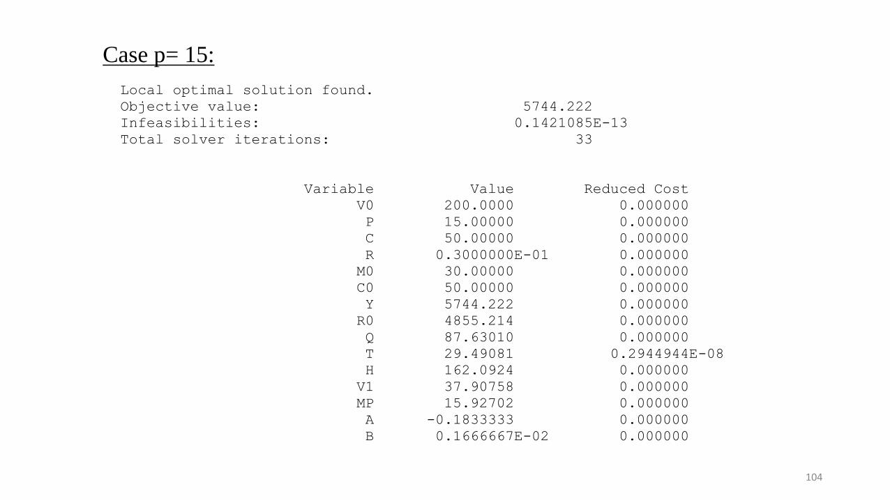
Case p= 15:
Local optimal solution found.
Objective value: 5744.222
Infeasibilities: 0.1421085E-13
Total solver iterations: 33
Variable Value Reduced Cost
V0 200.0000 0.000000
P 15.00000 0.000000
C 50.00000 0.000000
R 0.3000000E-01 0.000000
M0 30.00000 0.000000
C0 50.00000 0.000000
Y 5744.222 0.000000
R0 4855.214 0.000000
Q 87.63010 0.000000
T 29.49081 0.2944944E-08
H 162.0924 0.000000
V1 37.90758 0.000000
MP 15.92702 0.000000
A -0.1833333 0.000000
B 0.1666667E-02 0.000000

105
Case p = 25:
Local optimal solution found.
Objective value: 6485.002
Infeasibilities: 0.9094947E-12
Total solver iterations: 33
Variable Value Reduced Cost
V0 200.0000 0.000000
P 25.00000 0.000000
C 50.00000 0.000000
R 0.3000000E-01 0.000000
M0 30.00000 0.000000
C0 50.00000 0.000000
Y 6485.002 0.000000
R0 4412.308 0.000000
Q 58.10996 0.000000
T 17.22910 0.000000
H 139.5701 0.000000
V1 60.42991 0.2916067E-08
MP 23.12150 0.000000
A -0.1833333 0.000000
B 0.1666667E-02 0.000000
106
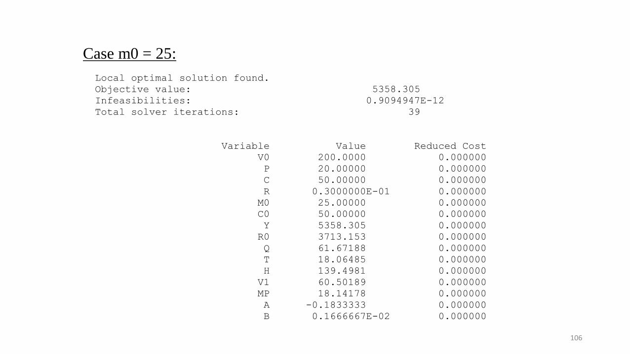
Case m0 = 25:
Local optimal solution found.
Objective value: 5358.305
Infeasibilities: 0.9094947E-12
Total solver iterations: 39
Variable Value Reduced Cost
V0 200.0000 0.000000
P 20.00000 0.000000
C 50.00000 0.000000
R 0.3000000E-01 0.000000
M0 25.00000 0.000000
C0 50.00000 0.000000
Y 5358.305 0.000000
R0 3713.153 0.000000
Q 61.67188 0.000000
T 18.06485 0.000000
H 139.4981 0.000000
V1 60.50189 0.000000
MP 18.14178 0.000000
A -0.1833333 0.000000
B 0.1666667E-02 0.000000
107
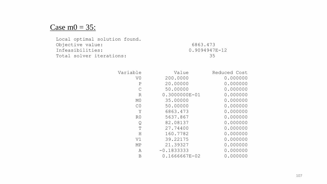
Case m0 = 35:
Local optimal solution found.
Objective value: 6863.473
Infeasibilities: 0.9094947E-12
Total solver iterations: 35
Variable Value Reduced Cost
V0 200.0000 0.000000
P 20.00000 0.000000
C 50.00000 0.000000
R 0.3000000E-01 0.000000
M0 35.00000 0.000000
C0 50.00000 0.000000
Y 6863.473 0.000000
R0 5637.867 0.000000
Q 82.08137 0.000000
T 27.74400 0.000000
H 160.7782 0.000000
V1 39.22175 0.000000
MP 21.39327 0.000000
A -0.1833333 0.000000
B 0.1666667E-02 0.000000
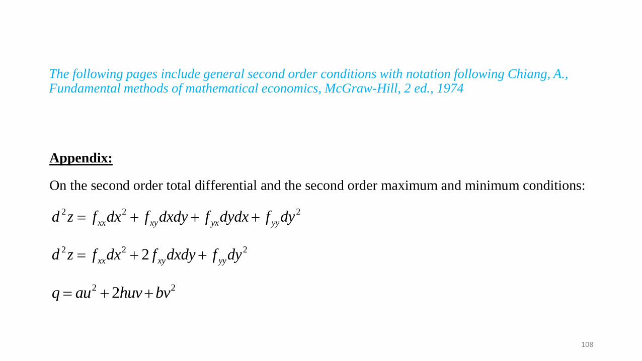
The following pages include general second order conditions with notation following Chiang, A., Fundamental methods of mathematical economics, McGraw-Hill, 2 ed., 1974
108
Appendix:
On the second order total differential and the second order maximum and minimum conditions:
2 2 2
xx xy yx yyd z f dx f dxdy f dydx f dy
2 2 22xx xy yyd z f dx f dxdy f dy
2 22q au huv bv

109
2 22q au huv bv
2 22 2 2 22
h hq au huv v bv v
a a
2 22 2 2
2
2h h hq a u uv v b v
a a a
2 22h ab h
q a u v va a

110
Results:
If: 20 0 0a ab h q , the quadratic form is said to be negative definite.
If: 20 0 0a ab h q , the quadratic form is said to be positive definite.
In other words: Assumption: A unique (local) maximum exists. The following conditions hold:
2 2
22 2
2 2 2 2
2
0, 0, 0
d f d f
dx dxdyd f d f
dx dy d f d f
dydx dy
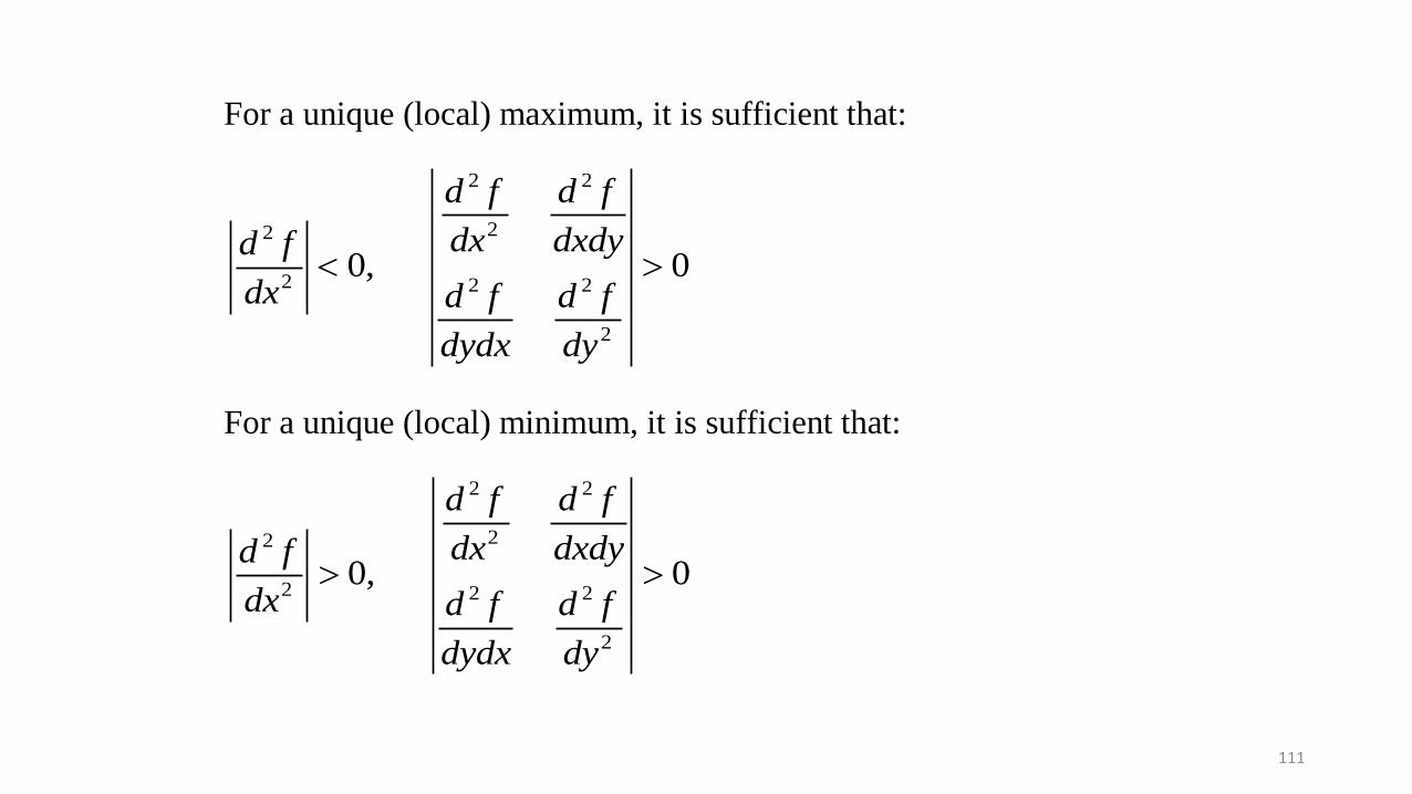
111
For a unique (local) maximum, it is sufficient that:
2 2
22
2 2 2
2
0, 0
d f d f
dx dxdyd f
dx d f d f
dydx dy
For a unique (local) minimum, it is sufficient that:
2 2
22
2 2 2
2
0, 0
d f d f
dx dxdyd f
dx d f d f
dydx dy

MATHEMATICAL APPENDIX to
Optimal continuous cover forest management:- Economic and environmental effects and legal considerations
Professor Dr Peter Lohmander http://www.Lohmander.com
BIT's 5th Low Carbon Earth Summit (LCES 2015 & ICE-2015)
Theme: "Take Actions for Rebuilding a Clean World"
September 24-26, 2015
Venue: Xi'an, China
112


![[Tabachnikov S.] Mathematical Methods of Classical(BookFi.org)](https://img.pdfslide.us/doc/110x75/577ccec41a28ab9e788e3f0c/tabachnikov-s-mathematical-methods-of-classicalbookfiorg.jpg)