NONLINEAR DYNAMIC INTERTWINING OF RODS WITH SELF-CONTACT

AUTHORS:

Sachin Goyal1(current), 2(work) (sgoyal@whoi.edu)

N. C. Perkins2 (ncp@umich.edu) – Corresponding Author

Christopher L. Lee3(current), 4(work) (christopher.lee@olin.edu)

AFFILIATIONS:

1Applied Ocean Physics and Engineering

Woods Hole Oceanographic Institution, Woods Hole MA 02543 (U.S.A.)

2Department of Mechanical Engineering

University of Michigan, Ann Arbor MI 48109 (U.S.A.)

3Department of Mechanical Engineering

Olin College, Needham, MA 02492 (U.S.A.)

4 Lawrence Livermore National Laboratory

New Technologies Engineering Division

7000 East Ave., Livermore, CA 94550 (U.S.A.)

1

ABSTRACT

Twisted marine cables on the sea floor can form highly contorted three-dimensional loops

that resemble tangles. Such tangles or ‘hockles’ are topologically equivalent to the

plectomenes that form in supercoiled DNA molecules. The dynamic evolution of these

intertwined loops is studied herein using a computational rod model that explicitly

accounts for dynamic self-contact. Numerical solutions are presented for an illustrative

example of a long rod subjected to increasing twist at one end. The solutions reveal the

dynamic evolution of the rod from an initially straight state, through a buckled state in the

approximate form of a helix, through the dynamic collapse of this helix into a near-planar

loop with one site of self-contact, and the subsequent intertwining of this loop with

multiple sites of self-contact. This evolution is controlled by the dynamic conversion of

torsional strain energy to bending strain energy or, alternatively by the dynamic

conversion of twist (Tw) to writhe (Wr).

KEY WORDS

Rod Dynamics, Self-contact, Intertwining, DNA Supercoiling, Cable Hockling

2

1. INTRODUCTION

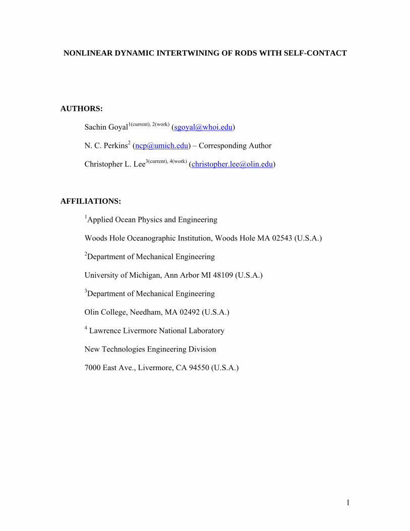
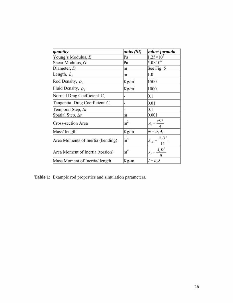
Cables laid upon the sea floor may form loops and tangles as illustrated in Fig. 1. The

loops, sometimes referred to as hockles, may cause localized damage and, in the case of

fiber optic cables, may also prevent signal transmission. These highly nonlinear

deformations are initiated by a combination of low tension or compression (i.e. cable

slack) and residual torsion sufficient to induce torsional buckling of the cable. Tangles

evolve from a subsequent dynamic collapse of the buckled cable into highly nonlinear

and intertwined configurations with self-contact.

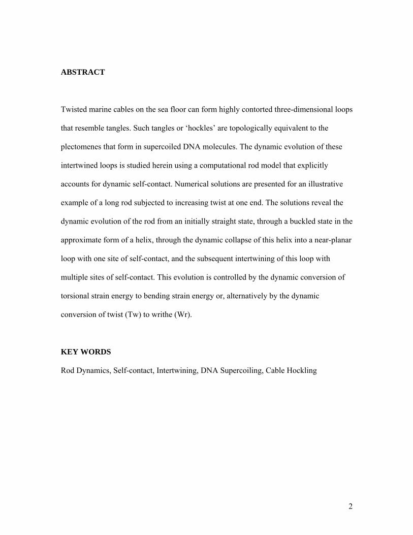
The looped and tangled forms of marine cables are topologically equivalent to the

‘plectonemic supercoiling’ of long DNA molecules as illustrated in Fig. 2 (refer to

Calladine et al. 2004; Goyal et al. 2005a). Figure 2 depicts a DNA molecule on three

different length scales as reproduced from (Branden & Tooze 1999; Lehninger et al.

2005). The smallest length scale (far left) shows a segment of the familiar ‘double-helix’

which has a diameter of approximately 2 nanometers (nm). One complete helical turn is

depicted here and this extends over a length of approximately 3 nm.

On an intermediate spatial scale (middle of Fig. 2), the double helix now appears as a

long and slender DNA molecule that might be realized when considering tens to

hundreds of helical turns (approximately tens to hundreds of nm). Two idealized ‘long-

length scale structures’ of DNA are illustrated to the far right in Fig. 2. Here, the

3

exceedingly long DNA molecule may contain thousands to millions of helical turns and

behave as a very flexible filament with lengths ranging from micron to millimeter scales

or even longer. The long-length scale curving and twisting of this flexible molecule is

referred to as supercoiling. Two generic types of supercoils are illustrated. A plectonemic

supercoil leads to an interwound structure where the molecule wraps upon itself with

many sites of apparent ‘self-contact’. By contrast, a solenoidal supercoil possesses no

self-contact and forms a secondary helical structure resembling a coiled spring or a

telephone cord.

Often with the aid of proteins, DNA must supercoil for several key reasons. First,

supercoiling provides an organized means to compact the very long molecule (by as

much as ) within the small confines of the cell nucleus. An unorganized compaction

would hopelessly tangle the molecule and render it useless as the medium for storing

genetic information. Second, supercoiling plays important roles in the transcription,

regulation and repair of genes. For instance, specific regulatory proteins are known to aid

or to hinder the formation of simple loops of DNA which in turn regulate gene activity;

refer, for example, to (Schleif 1992) and (Semsey et al. 2005).

510

Like the tangling of marine cables above, the intertwining of DNA is inherently a

nonlinear dynamic process controlled by structural properties (e.g., elasticity) and applied

forces (e.g., protein interactions). Rod theory provides a useful framework to explore the

dynamics of intertwining of long filament-like structures such as cables and DNA

molecules, as described, for example in (Goyal 2006). The mechanics of intertwining

4

immediately invokes formulations for self-contact in rod theory which remain a

significant challenge as emphasized recently in (Chouaieb et al. 2006; van der Heijden et

al. 2006).

The inclusion of self-contact in equilibrium formulations of rod theory has been treated in

(Coleman et al. 2000; Gonzalez et al. 2002; Schuricht & von der Mosel 2003; van der

Heijden et al. 2003; Coleman & Swigon 2004; Chouaieb et al. 2006; van der Heijden et

al. 2006). In particular, Chouaieb et al. (2006) evaluate helical equilibria where self-

contact is accounted for by imposing bounds on helical curvature and torsion. The

formation of self-contact in the equilibria generated from ‘closed’ or ‘circular’ rods (e.g.,

representative of DNA plasmids) is examined in (Coleman et al. 2000; Coleman &

Swigon 2004) using numerical energy minimization. The mathematical existence of such

solutions is deduced in (Gonzalez et al. 2002) by careful formulation of the geometric

excluded volume constraint on self-intersection. The excluded volume constraint is

formulated in terms rod of centerline curvature in (Schuricht & von der Mosel 2003) and

appended via Lagrange multiplier to the Euler-Lagrange equation for rod equilibrium

with self-contact. The analysis of ‘open’ rods (e.g., rods that do not close upon

themselves) requires consideration of two boundary conditions through which loads may

also be applied. A numerical study of the self-contacting equilibria of clamped-clamped

rods reveals the bifurcations generated by varying compression and twist applied at the

boundaries (van der Heijden et al. 2003). A recent extension (van der Heijden et al. 2006)

considers cases where the rod is constrained to lie on the surface of a cylinder. Open

questions regarding the analysis of rods with self-contact are emphasized in (van der

5

Heijden et al. 2006) by the lament “We are still far from understanding analytically the

solutions of the Euler-Lagrange equations for general contact situations. Even if we limit

ourselves to global minimizers of an appropriate energy functional, we can prove little

about the form of solutions as soon as contact is taken into account.”

In contrast to the equilibrium formulations above, very few dynamical formulations of

rod theory have been proposed that incorporate self-contact. Nevertheless, such

formulations enable one to explore the dynamic evolution of self-contacting states and

possible dynamic transitions between them. For instance, the slow twisting of the

filament treated in (Goyal et al. 2003b) ultimately induces a sudden dynamic collapse of

an intermediate helical loop into an intertwined form. An approximate dynamical

formulation is also presented in (Klapper 1996) where inertial effects are ignored in favor

of dissipation and stiffness effects.

In this paper, we revisit the slow twisting of a filament (Goyal et al. 2003b) with the

objective to develop a fundamental understanding of the dynamic evolution of its

intertwined states. In particular, we describe how intertwined states result from a sudden

collapse of helically-looped states through a rapid conversion of torsional to bending

strain energy. The remainder of this paper is organized as follows. Sections 2 and 3

summarize a computational dynamic rod model that incorporates self-contact (Goyal

2006). Section 4 presents an illustrative example of a non-homogeneous rod subject to

pure torsion. Results highlight the dynamic evolution from straight to looped to

6

intertwined states following a dramatic collapse to self-contact. We close in Section 5

with conclusions.

2. COMPUTATIONAL ROD MODEL – A SUMMARY

The rod segment illustrated in Fig. 3 is a thin (1-dimensional) element that may undergo

two-axis bending and torsion in forming a three-dimensional space curve. This curve

represents the rod centerline which, in the context of double-stranded DNA, represents

the helical axis of the duplex. We develop the dynamical model by employing the

classical approximations of Kirchhoff and Clebsch (Love 1944) as detailed in (Goyal

2006). A summary is provided here.

2.1 Rod Kinematics, Constitutive Law, and Energy

Consider the infinitesimal element of a Kirchhoff rod shown in Fig. 3. The three-

dimensional curve formed by the centerline is parameterized by the arc length

coordinate and time t . The body-fixed frame at each cross-section is employed to

describe the orientation of the cross-section with respect to the inertial frame . The

angular velocity

),( tsR

s }{ ia

}{ ie

),( tsω of the cross-section is defined as the rotation of the body-fixed

frame per unit time relative to the inertial frame and satisfies }{ ia }{ ie

i

e

i at

a

i

×=⎟⎠⎞

⎜⎝⎛∂∂

ω}{

, (1)

7

where the subscript specifies the reference frame relative to which the derivative has been

taken. We also define a ‘curvature and twist vector’ ),( tsκ as the rotation of the body-

fixed frame per unit arc length relative to the inertial frame which satisfies }{ ia }{ ie

i

e

i asa

i

×=⎟⎠⎞

⎜⎝⎛∂∂

κ}{

. (2)

In a stress-free state, the rod conforms to its natural geometry defined by )(0 sκ . The

difference { }0( , ) ( )s t sκ κ− results in an internal moment at each cross-section of

the rod. The relationship between the change in curvature/twist

),( tsq

{ }0( , ) ( )s t sκ κ− and the

restoring moment is governed by a constitutive law for bending and torsion.

While many generalizations of the constitutive law are discussed in (Goyal 2006), in this

study we employ the linear elastic law

),( tsq

))(),()((),( 0 stssBtsq κκ −= (3)

where is a positive definite stiffness tensor that is a prescribed function of position s.

The resulting strain energy density is

)(sB

))(),()(())(),((21),( 00 stssBststsS T

e κκκκ −−= . (4)

We further employ a diagonalized form of by choosing to coincide with the

‘principal torsion-flexure axes’ of the cross-section (Love 1944). In particular, and

)(sB }{ ia

1a 2a

8

are in the plane of the cross-section and are aligned with the principal flexure axes while

is normal to the cross-section and coincides with the tangent . The resulting

diagonal form of the stiffness tensor is

3a t̂

)(sB

⎥⎥⎥

⎦

⎤

⎢⎢⎢

⎣

⎡=

)(000)(000)(

)( 2

1

sCsA

sAsB , (5)

where and are bending stiffnesses about the principal flexure axes along

and respectively, and is the torsional stiffness about principal torsional or

‘tangent’ axis . Furthermore, in the results that follow, the rod is assumed to be

isotropic

)(1 sA )(2 sA 1a

2a )(sC

3a

1 but non-homogeneous (i.e. )()()( 21 sAsAsA == ). The stress-distribution at

any cross-section not only results in a net internal moment , but also net tensile and

shear forces .

),( tsq

),( tsf

The kinetic energy of the rod depends upon the centerline velocity and the cross-

section angular velocity

),( tsv

),( tsω . Let denote the mass of the rod per unit arc length

and denote the tensor of principal mass moments of inertia per unit arc length. Then

the rod kinetic energy density is

)(sm

)(sI

),()(),(21),()(),(

21),( tsvsmtsvtssItstsK TT

e += ωω . (6)

1 The rod is assumed to have circular cross section in this study with axi-symmetric bending stiffness.

9

We choose the vectors ,),( tsv ),( tsω , ),( tsκ and as four unknown field variables

in the formulation below. The kinematical quantities

),( tsf

),( tsκ , ),( tsω and can be

readily integrated to compute the rod configuration and the cross-section

orientation as given by ; refer to Fig. 3 and to (Goyal 2006).

),( tsv

),( tsR

)},({ tsai

Depending upon the application, the rod may also interact with numerous external field

forces including those produced by gravity, a surrounding fluid medium, electrostatic

forces, contact with other bodies or with the rod itself, , etc. The resultant of these

external forces and moments per unit length is denoted by and ,

respectively. In general, these quantities may be functionally-dependent on the

kinematical quantities

,...),( tsF ,...),( tsQ

),( tsκ , ),( tsω and in addition to the rod

configuration .

),( tsv

),( tsR

We next specify the four field equations required to solve for the four vector

unknowns },,,{ fv κω . In the field equations, we employ partial derivatives of all

quantities relative to the body-fixed frame and recall the following relations to the

partial derivatives relative to the inertial frame for a vector quantity

}{ ia

υ (Greenwood

1988):

υωυυ×−⎟

⎠⎞

⎜⎝⎛∂∂

=⎟⎠⎞

⎜⎝⎛∂∂

}{}{ ii ea tt and υκυυ

×−⎟⎠⎞

⎜⎝⎛∂∂

=⎟⎠⎞

⎜⎝⎛∂∂

}{}{ ii ea ss, (7)

For notational convenience, we drop the subscript for the body-fixed frame from this

point forward.

10

2.2 Equations of Motion

The balance law for linear momentum of the infinitesimal element shown in Fig. 3

becomes

Fv

tvmf

sf

−⎟⎠⎞

⎜⎝⎛ ×+∂∂

=×+∂∂ ωκ (8)

and that for angular momentum becomes

QtfIt

Iqsq

−×+×+∂∂

=×+∂∂ ˆωωωκ , (9)

Here, is the unit tangent vector along the centerline (directed towards increasing

arc length ) and the internal moment

),(ˆ tst

s ))(),()((),( 0 stssBtsq κκ −= upon substitution of

the constitutive law Eq. (3).

2.3 Constraints and Summary

The above formulation is completed with the addition of two vector constraints. The first

enforces inextensibility and unshearability which take the form

tvsv ˆ×=×+∂∂ ωκ . (10)

11

The second follows from continuity requirements for ω and κ in the form of the

compatibility constraint

ts ∂

∂=×+

∂∂ κωκω . (11)

Detailed derivations of these constraints are provided in (Goyal 2006).

The four vector equations Eq. (8-11) in the four vector unknowns },,,{ fv κω result in a

12th order system of nonlinear partial differential equations in space and time. They are

compactly written as

0),,(),,(),,( =/+∂∂

+∂∂ tsYF

sYtsYK

tYtsYM (12)

where },,,{),( fvtsY κω= and the operators M , K and F/ are described in ( Goyal et al.

2005b; Goyal 2006;). These equations are not integrable in general and thus we pursue a

numerical solution as detailed in (Goyal et al. 2005b; Goyal 2006). In particular, we

discretize the equations above by employing a finite difference algorithm using the

generalized-α method (Chung & Hulbert 1993) in both space and time. Doing so yields a

method that is unconditionally stable and second-order accurate. A single numerical

parameter can be varied to control maximum numerical dissipation. The difference

equations so obtained are implicit and their solution must satisfy the rod boundary

conditions. The boundary conditions are satisfied using a shooting method in conjunction

with Newton-Raphson iteration. In addition, this formulation also incorporates the forces

12

generated by self-contact which, being central to the objective of this paper, we describe

in some detail below.

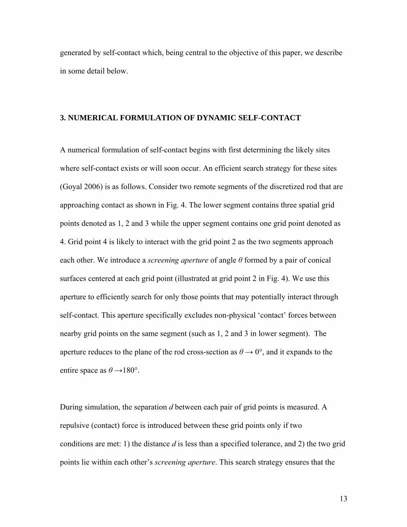
3. NUMERICAL FORMULATION OF DYNAMIC SELF-CONTACT

A numerical formulation of self-contact begins with first determining the likely sites

where self-contact exists or will soon occur. An efficient search strategy for these sites

(Goyal 2006) is as follows. Consider two remote segments of the discretized rod that are

approaching contact as shown in Fig. 4. The lower segment contains three spatial grid

points denoted as 1, 2 and 3 while the upper segment contains one grid point denoted as

4. Grid point 4 is likely to interact with the grid point 2 as the two segments approach

each other. We introduce a screening aperture of angle θ formed by a pair of conical

surfaces centered at each grid point (illustrated at grid point 2 in Fig. 4). We use this

aperture to efficiently search for only those points that may potentially interact through

self-contact. This aperture specifically excludes non-physical ‘contact’ forces between

nearby grid points on the same segment (such as 1, 2 and 3 in lower segment). The

aperture reduces to the plane of the rod cross-section as θ → 0°, and it expands to the

entire space as θ →180°.

During simulation, the separation d between each pair of grid points is measured. A

repulsive (contact) force is introduced between these grid points only if two

conditions are met: 1) the distance d is less than a specified tolerance, and 2) the two grid

points lie within each other’s screening aperture. This search strategy ensures that the

13

contact forces are approximately normal to the rod surfaces and also allows for sliding

contact. The interaction force can in general be a function of d and (the approach

speed) and it is included in the balance of linear momentum Eq. (8) through the

distributed force term F. Example interaction laws that can be employed include

(attractive-repulsive) Lennard-Jones type (refer to, for example (Schlick et al. 1994b)),

(screened repulsion) Debye-Huckle type (refer to, for example (Schlick et al. 1994a)),

general inverse-power laws (refer to, for example (Klapper 1996)), and idealized contact

laws for two solids (refer to, for example (van der Heijden et al. 2003) and (Coleman et

al. 2000)). In the specific case of DNA, one might introduce a fictitious charged and

cylindrical surface that circumscribes the molecule to capture the repulsive effects of the

negatively charged backbone.

d&

4. RESULTS

The computational model above is used to explore the dynamic evolution of an

intertwined state induced by slowly increasing the twist applied to one end of an elastic

rod. The numerical solutions reveals three major behaviors: 1) the torsional buckling of

an initially straight rod into the approximate shape of a helix, 2) the dramatic collapse of

this helix to a near-planar loop with self-contact at a single point, and 3) the subsequent

intertwining of the loop with multiple sites of self-contact.

14

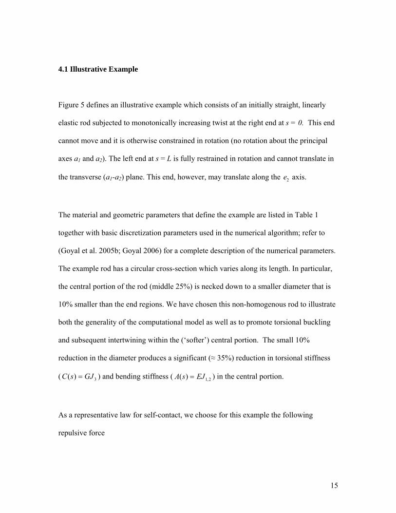
4.1 Illustrative Example

Figure 5 defines an illustrative example which consists of an initially straight, linearly

elastic rod subjected to monotonically increasing twist at the right end at s = 0. This end

cannot move and it is otherwise constrained in rotation (no rotation about the principal

axes a1 and a2). The left end at s = L is fully restrained in rotation and cannot translate in

the transverse (a1-a2) plane. This end, however, may translate along the axis. 2e

The material and geometric parameters that define the example are listed in Table 1

together with basic discretization parameters used in the numerical algorithm; refer to

(Goyal et al. 2005b; Goyal 2006) for a complete description of the numerical parameters.

The example rod has a circular cross-section which varies along its length. In particular,

the central portion of the rod (middle 25%) is necked down to a smaller diameter that is

10% smaller than the end regions. We have chosen this non-homogenous rod to illustrate

both the generality of the computational model as well as to promote torsional buckling

and subsequent intertwining within the (‘softer’) central portion. The small 10%

reduction in the diameter produces a significant (≈ 35%) reduction in torsional stiffness

( ) and bending stiffness (3)( GJsC = 2,1)( EJsA = ) in the central portion.

As a representative law for self-contact, we choose for this example the following

repulsive force

15

⎟⎟⎠

⎞⎜⎜⎝

⎛+

−=

4

2

31

)5.0(k

kcccontact dddk

Ddk

AF &&ρ , (13)

with example parameters: k1 = 10-7m4/s2, k2 = 3, k3 = 10-6 and k4 = 1. This contact law is

one of many possible that capture both nonlinear repulsion and dissipation. The results

that follow are rather insensitive to changes in the specific parameter values selected for

this example.

In addition to the contact law above, the only other body force considered is a dissipative

force. As one example, we introduce the viscous drag imparted by a surrounding fluid

environment in the form of the standard Morison drag law (Morison et al. 1950). This

distributed drag, which manifests itself in the balance of linear momentum Eq. (8)

through the distributed force term , is computed as (Goyal et al. 2005b): F

( ) ( ){ ttvtvCtvttvCDF tnfdragˆˆˆˆˆˆ

21

⋅⋅+×××−= πρ }, (14)

Here, is the normal (form) drag coefficient, is the tangential (skin friction) drag

coefficient, and

nC tC

fρ is fluid density. Example values of these parameters are reported in

Table 1.

4.2 Evolution of Self-Contact and Intertwining

By increasing the rotation (twist) slowly at the right end, the internal torque eventually

reaches the bifurcation condition associated with the classical torsional buckling of a

16

straight rod (Zachmann 1979). This rotation is generated by prescribing the angular

velocity component ω3 at the right end as shown in Fig. 6 (not to scale). In addition, the

left end is allowed to translate freely during the first 30 seconds and is then held fixed to

control what would otherwise be an exceedingly rapid collapse to self-contact as

described in the following.

As the right end is initially twisted by a modest amount, the rod remains straight. There is

an abrupt change however when the twist reaches the bifurcation value associated with

the Zachmann buckling condition (Zachmann 1979) and the straight (trivial)

configuration becomes unstable. This occurs at approximately 16 seconds in this

example. The computational model captures this initial instability as well as the

subsequent nonlinear motion that leads to loop formation and ultimately to intertwining.

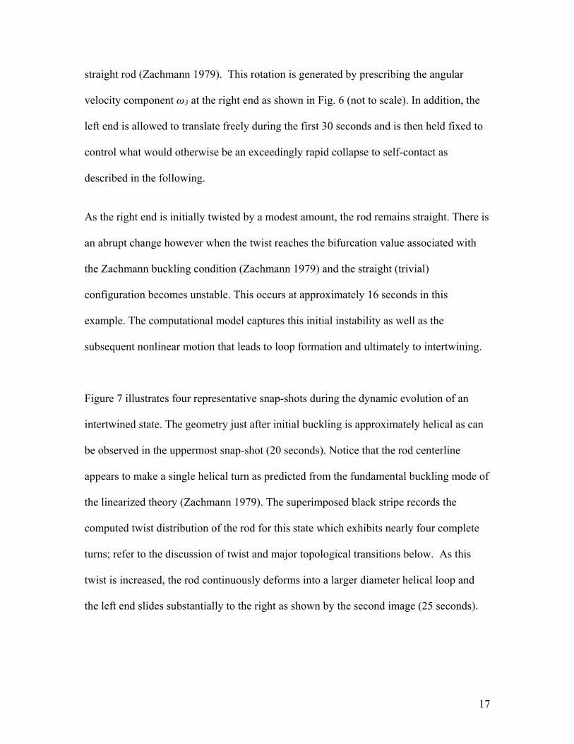
Figure 7 illustrates four representative snap-shots during the dynamic evolution of an

intertwined state. The geometry just after initial buckling is approximately helical as can

be observed in the uppermost snap-shot (20 seconds). Notice that the rod centerline

appears to make a single helical turn as predicted from the fundamental buckling mode of

the linearized theory (Zachmann 1979). The superimposed black stripe records the

computed twist distribution of the rod for this state which exhibits nearly four complete

turns; refer to the discussion of twist and major topological transitions below. As this

twist is increased, the rod continuously deforms into a larger diameter helical loop and

the left end slides substantially to the right as shown by the second image (25 seconds).

17

Upon greater twist, the left end continues to slide towards the right end and the helical

loop continues to rotate out of the plane of this figure. Eventually the loop undergoes a

secondary bifurcation followed by a rapid dynamic collapses into self-contact in forming

a nearly planar loop. The collapsed loop is shown by the third image (which occurs at

approximately 29 seconds).

The dynamic collapse can be anticipated from stability analyses of the equilibrium forms

of a rod under similar loading conditions; refer to (Lu & Perkins 1994) and studies cited

therein. The snap-shot at 25 seconds shows the three-dimensional shape of the rod just

prior to dynamic collapse. Here, the apex of the loop has rotated approximately 90° about

the vertical (e1) axis so that the tangent at the apex is now orthogonal to the loading (e2)

axis. This was the noted secondary bifurcation condition in (Lu & Perkins 1994) at which

the three-dimensional equilibrium form loses stability.

The collapsed loop, however, is very sensitive to the increasing twist and rapidly

continues to rotate about the vertical (e1) axis leading to intertwined forms with multiple

sites of self-contact. A snapshot of a fully intertwined loop is illustrated at the bottom of

Fig. 7 (32 seconds). The strain energy density (color scale in Fig. 7) reveals that the

strain energy becomes highly localized to the apex of the intertwined loop where the

curvature is greatest. The decomposition of this strain energy into bending and torsional

components provides significant insight into the dynamic evolution of an intertwined

state as discussed next.

18

4.3 Energetic Transitions

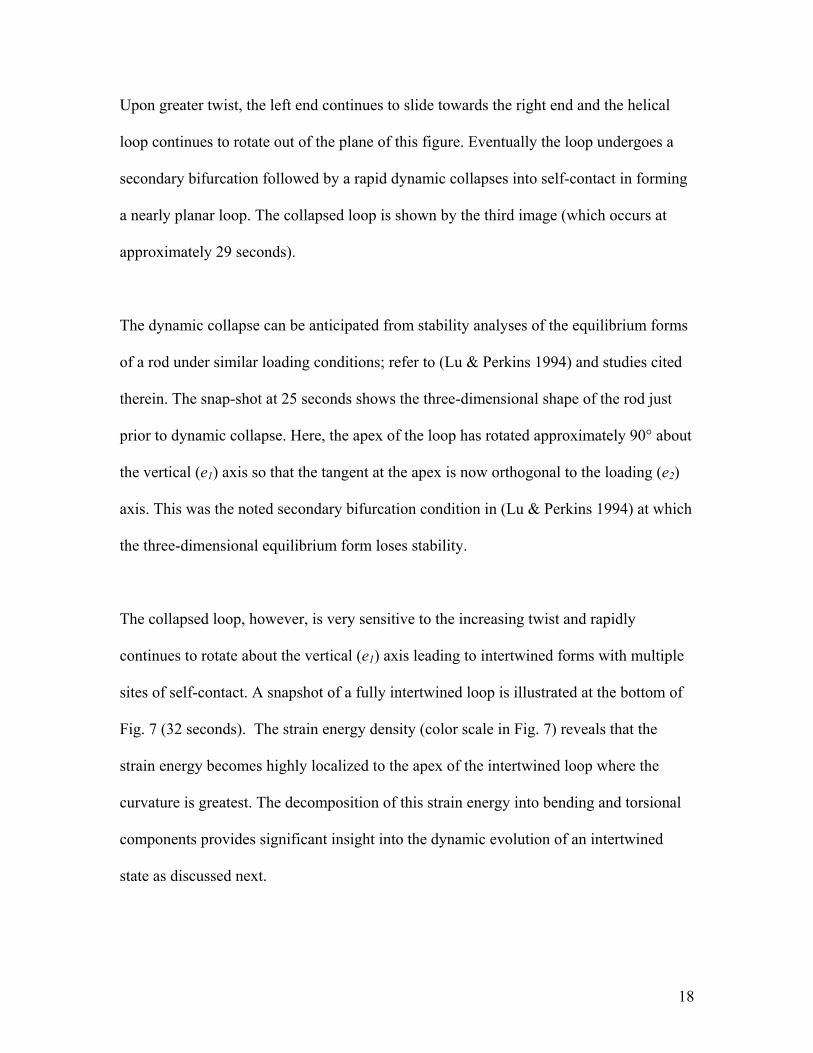
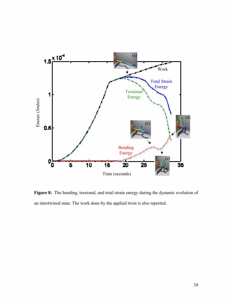
Figure 8 summarizes the energetics of this process by illustrating how the bending and

torsional strain energy components contribute to the total strain energy. Starting at time

zero, the initially straight rod remains straight and the applied twist simply increases the

torsional strain energy. This elementary, pure-twisting of the straight rod ceases at

approximately 18 seconds with the first bifurcation due to torsional buckling (Zachmann

1979). The torsional strain energy achieves its maximum at this state and immediately

thereafter the rod buckles into a three-dimensional form resembling a shallow helix (a).

This transition is accompanied by a conversion of torsional to bending strain energy. This

conversion is dynamic and markedly increases as the rod is twisted further while

developing a distinctive loop (b). The apex of this loop rotates further out of plane during

this stage. Just prior to 29 seconds the apex becomes orthogonal to the loading axis

(original axis of the straight rod) which marks the secondary bifurcation (Lu & Perkins

1994) that generates an extremely fast dynamic collapse to self-contact. The resulting

loop with self-contact is nearly planar (c). During this secondary bifurcation, the rod

loses both torsional and bending strain energies until self-contact and, thereafter

intertwining begins. As intertwining advances (d), the torsional strain energy continues

to decrease while the bending strain energy increases once more. In addition, the bending

strain energy becomes localized to the apex of the loop due to the significant and

increasing curvature developed there; refer also to snapshot at 32 seconds in Fig. 7. In

the case of DNA forming plectonemes, such localized strain energy might possibly be the

19

forerunner of the nonlinear ‘kinking’ of the molecule as proposed recently (Wiggins et al.

2005). Figure 8 also illustrates the total strain energy and the work done by twisting the

right boundary. The energy difference between the work done and the total strain energy

derives from the significant kinetic energy during this process as well as the dissipation

developed from the included fluid drag.

4.4 Topological Transitions

It is interesting to observe that the topological changes for the example rod above are also

exhibited by DNA during supercoiling. As discussed in (Calladine et al. 2004), the above

conversion of torsional strain energy to bending strain energy for DNA is more

frequently described topologically as the conversion of twist to writhe. We explore this

conversion in the above example after briefly reviewing the definitions for twist and

writhe.

Twist (Tw) is a kinematical quantity representing the total number of twisted turns along

the rod centerline as computed from

( )∫ ⋅=CL

dstTw0

ˆ21 κπ

(15)

Writhe (Wr) is defined as the average number of cross-overs of the rod centerline when

observed over all possible views of the rod (Calladine et al. 2004). For our initially

straight configuration, Wr = 0. At the first self-contact shown by the snapshot at 29

20

seconds in Fig. 7, Wr = 1. The writhe then continues to increase to Wr = 2 for the

intertwined state at 32 seconds in Fig. 7. The writhe is purely a function of the space

curve defining the rod centerline and it may also be positive or negative depending on

whether the crossing is right-handed or left-handed (Calladine et al. 2004). In our

illustrative example, the sum Tw + Wr equals the number of rotations of the right

boundary and this sum is called the Linking number Lk2. Refer to Fuller (Fuller 1971)

and White (White 1969) for the proof of conservation of the Linking number (Lk).

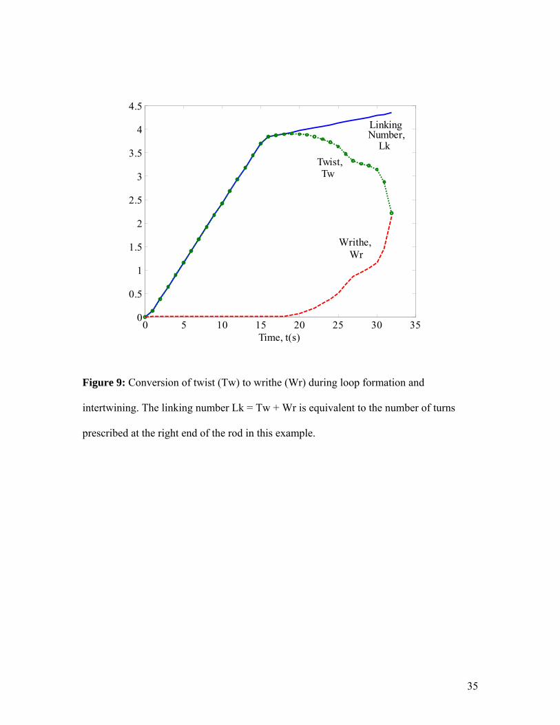
In our example, the initial twisting phase rapidly increases Lk from 0 to approximately 4,

all in the form of twist, prior to the first bifurcation (torsional buckling) as illustrated in

Fig. 9. An additional increase in Lk (end rotation) of less than ½ (turn) produces all of the

sudden transitions noted above. Following the first bifurcation, Wr increases from 0 to 1

at self-contact (29 seconds) and Tw correspondingly reduces so that the sum Wr + Tw

remains equal to Lk. Following the first self-contact, the loop continues to rotate as it

intertwines. In doing so, every half rotation of the loop establishes an additional contact

site thereby increasing Wr by 1 and reducing Tw by 1. At 32 seconds, Wr is slightly

larger than 2. Thus, we observe two crossovers in any three orthogonal views of the snap-

shot at 32 seconds shown in Fig. 7. There is a compensatory loss in Tw as shown in Fig.

9.

It should also be noted if self-contact is ignored, as has often been done in some prior

studies of the looping of rods, the numerical solution for the rod may allow it to

2 This is not true, in general, for other boundary conditions that allow rotations about the other axes (i.e., cases where ω1,2 ≠ 0 at the boundaries).

21

artificially ‘cut through itself’ leading to entirely different and non-physical results.

Following each ‘cut’, both Wr and Lk are reduced discontinuously by 2. Examples of this

readily follow from the present computational formulation by simply eliminating the

contact force. However, doing so leads to non-physical discontinuous changes in Wr and

Lk following artificial ‘cuts’ through the rod. Thus, modeling self-contact is

fundamentally necessary when one endeavors to understand the pathway(s) leading to the

intertwined loops.

5. CONCLUSIONS

This paper summarizes a computational rod model that captures the dynamical evolution

of intertwined loops in rods under torsion. A major feature is the explicit formulation of

dynamic self-contact. An illustrative example is selected which reveals a fundamental

understanding of how loops first form, then collapse, and then intertwine. This

knowledge may also promote an understanding of how long cables form ‘hockles’ and

how DNA molecules form plectonemic supercoils.

Numerical simulations reveal that an originally straight rod undergoes two bifurcations in

succession as twist is added. The first bifurcation is elementary and occurs at the

(Zachmann) buckling condition where the trivial equilibrium becomes unstable and the

rod buckles into the approximate shape of a shallow helix. Upon increasing twist, this

helix grows in amplitude to form a distinctive loop. In doing so, the apex of this loop

22

continues to rotate towards the out-of-plane direction. When the apex ultimately

becomes orthogonal to the loading axis (axis of the original straight rod), the loop

experiences a secondary bifurcation and a sudden dynamic collapse into a near-planar

loop with self-contact. As twist is again added, the near-planar loop rotates upon itself

becoming intertwined with multiple sites of self-contact. The energetics leading to the

intertwined form confirm the large exchange of torsional strain energy for bending strain

energy which becomes increasingly localized to the apex of the loop. These transitions

parallel the dynamic conversion of twist (Tw) to writhe (Wr) during this process.

ACKNOWLEDGEMENTS

The authors (NCP and SG) gratefully acknowledge the research support provided by the

U.S. Office of Naval Research (grant N00014-00-1-0001), the Lawrence Livermore

National Laboratories (grant B 531085), and the U. S. National Science Foundation

(grants CMS 0439574 and CMS 0510266). The author (CLL) performed work under the

auspices of the U.S. Department of Energy by the University of California, Lawrence

Livermore National Laboratory under contract No.W-7405-ENG-48.

23

REFERENCES

Branden, C. & Tooze, J. 1999 Introduction to protein structure. New York: Garland Publishing.

Calladine, C. R., Drew, H. R., Luisi, B. F. & Travers, A. A. 2004 Understanding DNA, the molecule and how it works. Amsterdam: Elsevier Academic Press.

Chouaieb, N., Goriely, A. & Maddocks, J. H. 2006 Helices. Proc. Natl. Acad. Sci. U. S. A. 103, 9398-9403.

Chung, J. & Hulbert, G. M. 1993 A time integration algorithm for structural dynamics with improved numerical dissipation - the generalized-alpha method. ASME J. Appl. Mech. 60, 371-375.

Coleman, B. D., Swigon, D. & Tobias, I. 2000 Elastic stability of DNA configurations. II. supercoiled plasmids with self-contact. Phys. Rev. E 61, 759-770.

Coleman, B. D. & Swigon, D. 2004 Theory of self-contact in Kirchhoff rods with applications to supercoiling of knotted and unknotted DNA plasmids. Phil. Trans. Roy. Soc. Lond. A 362, 1281-1299.

Fuller, F. B. 1971 Writhing number of a space curve. Proc. Natl. Acad. Sci. U. S. A. 68, 815-819.

Gonzalez, O., Maddocks, J. H., Schuricht, F. & von der Mosel, H. 2002 Global curvature and self-contact of nonlinearly elastic curves and rods. Calculus of Variations and Partial Differential Equations 14, 29-68.

Goyal, S., Perkins, N. C. & Lee, C. L. 2003b Writhing dynamics of cables with self-contact. Proceedings of Fifth International Symposium on Cable Dynamics, 27-36. Santa Margherita Ligure, Italy.

Goyal, S., Lillian, T., Perkins, N. C. & Meyhofer, E. 2005a Cable dynamics applied to long-length scale mechanics of DNA. (CD-ROM) Proceedings of Sixth International Symposium on Cable Dynamics. Charleston, South Carolina.

Goyal, S., Perkins, N. C. & Lee, C. L. 2005b Nonlinear dynamics and loop formation in Kirchhoff rods with implications to the mechanics of DNA and cables. J. Comput. Phys. 209, 371-389.

Goyal, S. 2006 A dynamic rod model to simulate mechanics of cables and DNA. Doctoral. Dissertation, The University of Michigan, Ann Arbor, Michigan.

Greenwood, D. T. 1988 Principles of dynamics. Englewood Cliffs, N.J. Prentice-Hall. Klapper, I. 1996 Biological applications of the dynamics of twisted elastic rods. J.

Comput. Phys. 125, 325-337. Lehninger, A. L., Nelson, D. L. & Cox, M. M. 2005 Lehninger principles of

biochemistry. New York: W. H. Freeman. Love, A. E. H. 1944 A Treatise on the mathematical theory of elasticity. New York:

Dover Publications. Lu, C. L. & Perkins, N. C. 1994 Nonlinear spatial equilibria and stability of cables under

uniaxial torque and thrust. ASME J. Appl. Mech. 61, 879-886.

24

Morison, J. R., Obrien, M. P., Johnson, J. W. & Schaaf, S. A. 1950 The force exerted by surface waves on piles. Trans. Am. Inst. Min. Metall. Eng. 189, 149-154.

Schleif, R. 1992 DNA looping. Annu. Rev. Biochem. 61, 199-223. Schlick, T., Li, B. & Olson, W. K. 1994a The influence of salt on the structure and

energetics of supercoiled DNA. Biophys. J. 67, 2146-2166. Schlick, T., Olson, W. K., Westcott, T. & Greenberg, J. P. 1994b On higher buckling

transitions in supercoiled DNA. Biopolymers 34, 565-597. Schuricht, F. & von der Mosel, H. 2003 Euler-Lagrange equations for nonlinearly elastic

rods with self-contact. Arch. Ration. Mech. Anal. 168, 35-82. Semsey, S., Virnik, K. & Adhya, S. 2005 A gamut of loops: meandering DNA. Trends

Biochem. Sci. 30, 334-341. van der Heijden, G. H. M., Neukirch, S., Goss, V. G. A. & Thompson, J. M. T. 2003

Instability and self-contact phenomena in the writhing of clamped rods. Int. J. Mech. Sci. 45, 161-196.

van der Heijden, G. H. M., Peletier, M. A. & Planque, R. 2006 Self-contact for rods on cylinders. Arch. Ration. Mech. Anal. 182, 471-511.

White, J. H. 1969 Self-linking and Gauss-integral in higher dimensions. Am. J. Math. 91, 693-728.

Wiggins, P. A., Phillips, R. & Nelson, P. C. 2005 Exact theory of kinkable elastic polymers. Phys. Rev. E 71.

Zachmann, D. W. 1979 Non-linear analysis of a twisted axially loaded elastic rod. Quart. Appl. Math. 37, 67-72.

25

quantity units (SI) value/ formula Young’s Modulus, E Pa 1.25×107 Shear Modulus, G Pa 5.0×106 Diameter, D m See Fig. 5 Length, cL m 1.0 Rod Density, cρ Kg/m3 1500 Fluid Density, fρ Kg/m3 1000 Normal Drag Coefficient nC - 0.1 Tangential Drag Coefficient tC - 0.01 Temporal Step, ∆t s 0.1 Spatial Step, ∆s m 0.001

Cross-section Area m2 4

2DAcπ

=

Mass/ length Kg/m cc Am ρ=

Area Moments of Inertia (bending) m4 16

2

2,1DA

J c=

Area Moment of Inertia (torsion) m4 8

2

3DA

J c=

Mass Moment of Inertia/ length Kg-m JI cρ=

Table 1: Example rod properties and simulation parameters.

26

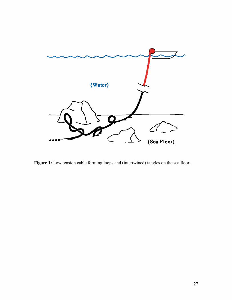
Figure 1: Low tension cable forming loops and (intertwined) tangles on the sea floor.

27

Figure 2: DNA shown on three length scales. Smallest scale (left) shows a single helical

repeat of the double-helix structure (sugar-phosphate chains and base-pairs). Intermediate

scale (middle) suggests how many consecutive helical repeats form the very long and

slender DNA molecule. Largest scale (right) shows how the molecule ultimately curves

and twists in forming supercoils (plectonemic or solenoidal). (Courtesy: (Branden &

Tooze 1999) and (Lehninger et al. 2005)).

28

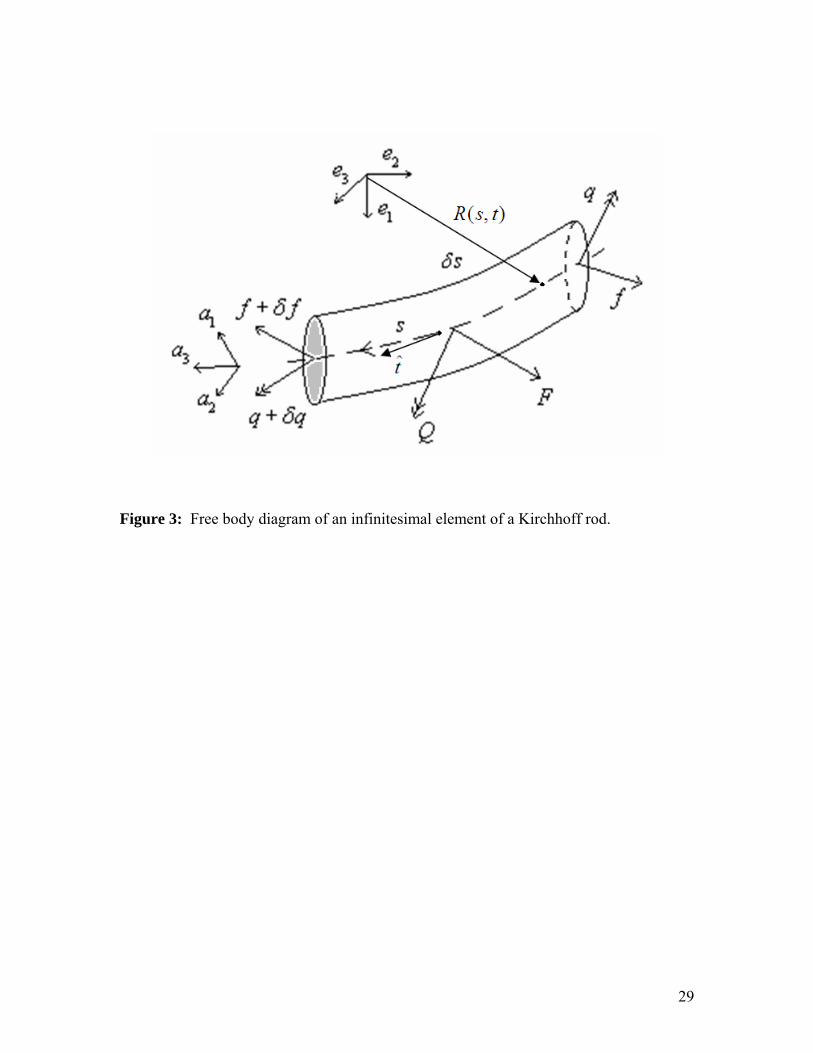
Figure 3: Free body diagram of an infinitesimal element of a Kirchhoff rod.

29

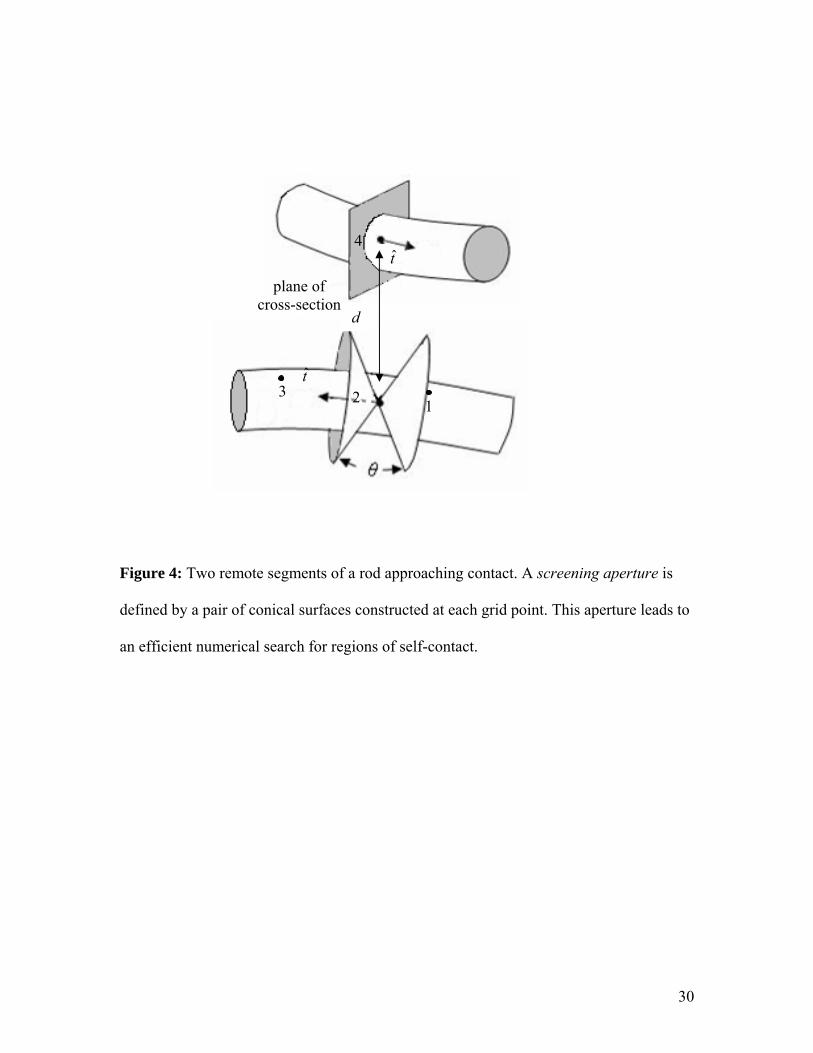
Figure 4: Two remote segments of a rod approaching contact. A screening aperture is

defined by a pair of conical surfaces constructed at each grid point. This aperture leads to

an efficient numerical search for regions of self-contact.

d

t̂

t̂

cross-section

4

plane of

3 2 1

30

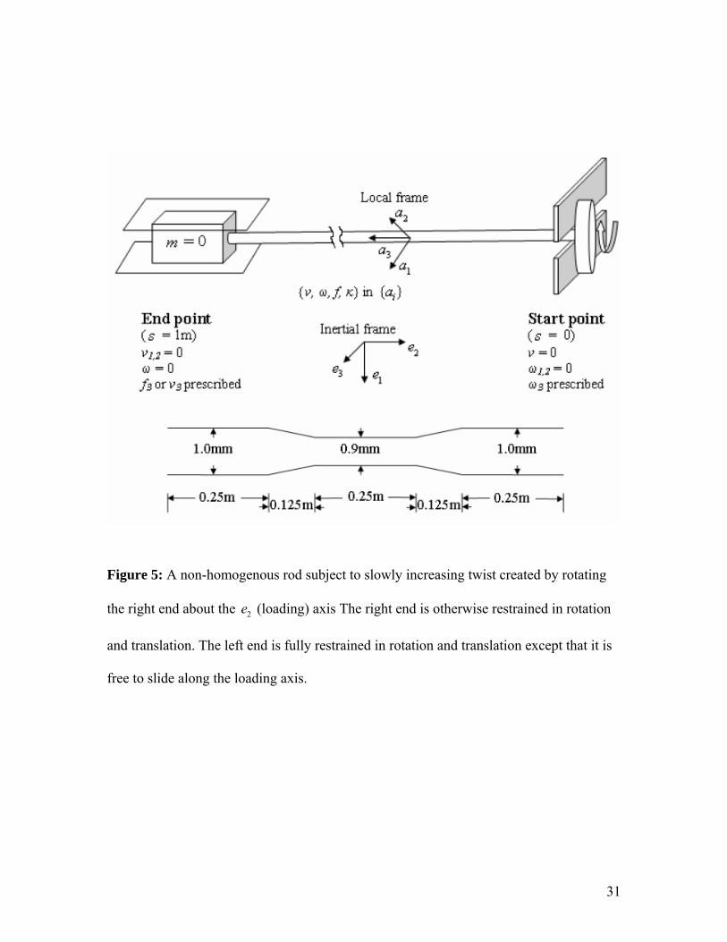
Figure 5: A non-homogenous rod subject to slowly increasing twist created by rotating

the right end about the (loading) axis The right end is otherwise restrained in rotation

and translation. The left end is fully restrained in rotation and translation except that it is

free to slide along the loading axis.

2e

31

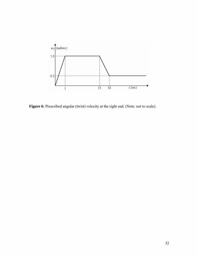
Figure 6: Prescribed angular (twist) velocity at the right end. (Note: not to scale).

32

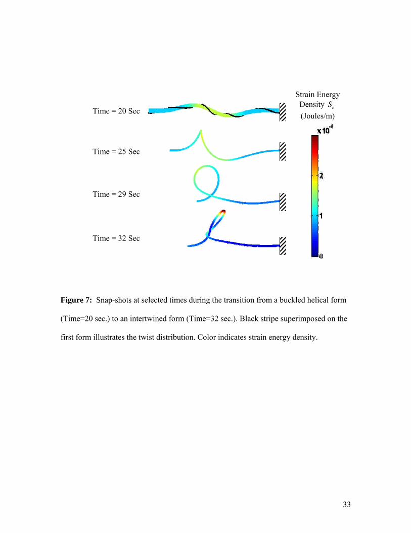
Figure 7: Snap-shots at selected times during the transition from a buckled helical form

(Time=20 sec.) to an intertwined form (Time=32 sec.). Black stripe superimposed on the

first form illustrates the twist distribution. Color indicates strain energy density.

Time = 20 Sec

Time = 25 Sec

Time = 29 Sec

Time = 32 Sec

Strain Energy Density (Joules/m)

eS

33

Time (seconds)

Work

Torsional Energy

(c)

(b)

Bending Energy

Total Strain Energy

(d)

Ener

gy (J

oule

s)

(a)

Figure 8: The bending, torsional, and total strain energy during the dynamic evolution of

an intertwined state. The work done by the applied twist is also reported.

34

0 5 10 15 20 25 30 350

0.5

1

1.5

2

2.5

3

3.5

4

4.5

Time, t(s)

LinkingNumber,

LkTwist,Tw

Writhe,Wr

Figure 9: Conversion of twist (Tw) to writhe (Wr) during loop formation and

intertwining. The linking number Lk = Tw + Wr is equivalent to the number of turns

prescribed at the right end of the rod in this example.

35