Algorithms for Finite Fields

1 Introduction

This course will discuss efficient ways to do computations over finite fields.First, we will search for efficient ways to factor polynomials over finite fields.There is a probabilistic polynomial time algorithm for this, as we’ll see.Second, we’ll discuss computations involving discrete logarithms. That is,suppose h ∈< g >, find n such that h = gn. As of the first class day, thereis no polynomial time algorithm for this problem. It is possible that thereis no such algorithm. Third, we will look at primality testing for integers.There is a deterministic polynomial time algorithm for this problem, and itis essentially a finite field algorithm. It starts with a ring depending of thenumber to be tested, which is a field if and only if the number is prime.

For every prime number p and positive integer n, there exists a fieldwith pn elements, and any two such fields are isomorphic. Fpn denotes“the” finite field with pn elements. When n = 1, we have Fp = Z/pZ. Oneway of describing Fpn is as the splitting field of xpn − x in the algebraicclosure of Fp. This is unsatisfactory, however, since this does not show howto compute the algebraic closure. A better way is to choose an irreduciblef(x) ∈ Fp[x] of degree n and think of Fpn as Fp[x]/(f(x)). This is bettersince we may describe each element in this field as a0 +a1x+ . . .+an−1x

n−1

for ai ∈ Fp. But, we have a new problem on our hands: Given p and n, findan irreducible polynomial of degree n in Fp[x]. We would like the fastestpossible procedure for this, i.e. one that is polynomial in nlog p. Indeed,we cannot do better than nlogp, since for f(x) = f0 + f1x + . . . + fnxn wewould need log p digits just to describe each fi.

Example 1 (Easy) If n = 2 and p ≡ 3(mod 4), then f(x) = x2 + 1 isgood.

Example 2 (Hard) Same n = 2 but with p ≡ 1(mod 4).

How likely is a polynomial of degree n picked at random irreducible?Over Fp, the probability is 1/n. So, our algorithm is simple: pick a randompolynomial of degree n, and test whether it is irreducible. If it is, great. Ifnot, pick another.

Now, suppose you are lucky and find two irreducible polynomials f(x)and g(x) of degree n. Then Fp[x]/(f(x)) ∼= Fp[x]/(g(x)). A natural questionto ask is, what is the isomorphism? There is a deterministic polynomial time

1

algorithm for finding this; so now that we know the ending, we’ll move alongto the next example.

We know that F×q = Fq − {0} is a cyclic group of order q − 1, but whatis the generator? One algorithm to find it is to pick g ∈ F×q at random, andcheck if g(q−1)/l 6= 1 for all primes l|(q−1). It is clear that this is a necessaryand sufficient condition for g to generate F×q . This is not hard to do providedwe have a factorization of q − 1. (If we know the factorization, then this isa probabilistic polynomial time algorithm for finding the generator.) Thenumber of generators is φ(q−1), so the probability that an element chosen atrandom is a generator is φ(q− 1)/q− 1. This algorithm is efficient for smallq, but for large q, we’d like to have a smaller set from which to search forour generator, as opposed to picking from all of F×q . Under the generalizedRiemann Hypothesis, there is a g such that 2 < g < (log p)2 which is aprimitive root mod p. It may be (log p)3, or something close to that, but thepoint is that it is very specific. So, we have a deterministic algorithm if wepick sequentially, but we must assume the generalized Riemann Hypothesis.

Example 3 Look at Fpp = Fp[x]/(xp − x− 1). F×pp has pp − 1 elements,and pp − 1 = (p− 1)pp−1

p−1 . We have an exact sequence:

1 −→ F×p −→ F×pp −→ G −→ 1.

Ker NFpp/Fpis a subgroup of F×pp of order pp−1

p−1 splitting the exact sequence.

Conjecture: The image of x in Fp[x]/(xp−x−1) has order pp−1p−1 . (Only

been checked for primes less than 20.)Given a ground field Fq, if we want to build an extension of degree n we

need an irreducible polynomial f(x) of degree n so that Fqn = Fq[x]/(f(x)).We shall now study some algorithms in Fq[x] with a view towards an irre-ducibility test.

Division Algorithm

Given polynomials a(x), f(x) ∈ Fq[x] ∃ polynomials b(x), r(x) ∈ Fq[x] suchthat

1. a(x) = b(x)f(x) + r(x)

2. deg r(x) < deg f(x)

2

Algorithm

Let a = a0xm + . . . and f = f0x

n + . . . .If deg a < deg f ⇒ b = 0, r = aElse if deg a = m > deg f = nReplace a by a− a0

f0xm−nf and b by b + a0

f0xm−n

Do this until deg a < deg f .

This algorithm takes at most m − n steps to get b and r. Each step takesO(n) operations in Fq and the whole process takes O(mn) operations.

Euclidean Algorithm

Given polynomials a, b ∈ Fq[x] with deg b 6 deg a we want to computegcd(a, b). We shall let a%f denote the remainder when a is divided by f .

Algorithm

gcd(a, b) = gcd(b, a%b)Do this until gcd(a, 0) = a

Iterating will compute gcd(a, b) in O(max{deg a,deg b}) = O(deg a) divi-sion of polynomials.

Raising to an integral power

Given a, f ∈ Fq[x] and m > 0 an integer we would like to compute am mod f .This can be done in O(log m) operations in Fq[x]/(f(x)).

Algorithm

Let us look at the binary expansion of m.

m = m0 + m12 + · · ·+ mr2r,mi ∈ {0, 1}

To improve efficiency of our algorithm we could use the base p representationof m.We compute by squaring and then reducing mod p the previous term of thesequence.

{a, a2, . . . a2r}

3

Then am = am0(a2)m1 · · · (a2r)mr can be computed by using at most r + 1

multiplications from terms of the sequence.Since we are reducing mod f each time the degree of a does not becomelarge.

Irreducibility of Polynomials

Theorem 1. Let f(x) ∈ Fq[x] be a polynomial of degree n. Then f(x) isirreducible iff

1. f(x)|(xqn − x)

2. gcd(f(x), xqd − x) = 1, ∀ d|n, d < n

Proof. Assume 1 and 2.1⇒ f splits completely in Fqn and has simple roots.2⇒ f has no roots in a smaller subextension of Fqn/Fq

So f is irreducible, since a factor would have to have roots in a field smallerthan Fqn . Converse is similar.

Algorithm

We want to compute (xqd − x)%f .We compute xqd

in Fq[x]/(f(x)) which takes at most d log q steps.xqd ≡ b mod f (deg b < deg f) .(xqd − x)%f = (b− x)%fWhen d = n this is item 1 of the theorem. For d < n this calculation isthe first step of the Euclidean Algorithm. Subsequent steps involve onlypolynomials of degree at most n.

Example 1. Consider f(x) = x5 + x + 1 in F2[x].Condition 2 of the Theorem is clearly satisfied i.e. gcd(f(x), x2 − x) = 1.We want to compute x25

mod f .x, x2, x4

x8 ≡ x4 + x3 mod f

x16 ≡ x8 + x6 ≡ x4 + x3 + x2 + x mod f

x32 ≡ x8 + x6 + x4 + x2

≡ x4 + x3 + x2 + x4 + x2 ≡ x3 + x mod f

Hence (x32 − x)%f = x3 6= 0 and hence condition 1 of the Theorem is notsatisfied. So f is reducible.

4

For large q and small n there might be better algorithms.We have a fast deterministic test for irreducibility of polynomials over

finite fields. How do we find an irreducible polynomial of given degree nover Fq? There is no deterministic polynomial time algorithm to do this.There is a probabilistic algorithm.

Algorithm

Pick a monic polynomial f(x) ∈ Fq[x] of degree n at random. Test forirreducibility. Repeat until you find an irreducible polynomial.

The algorithm is based on the following theorem.

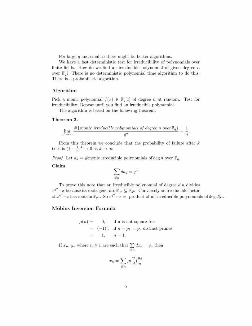
Theorem 2.

limqn→∞

#{monic irreducible polynomials of degree n over Fq}qn

=1n

.

From this theorem we conclude that the probability of failure after ktries is (1− 1

n)k → 0 as k →∞

Proof. Let ad = #monic irreducible polynomials of deg n over Fq.

Claim. ∑d|n

dad = qn

To prove this note that an irreducible polynomial of degree d|n dividesxqn−x because its roots generate Fqd ⊆ Fqn . Conversely an irreducible factorof xqn−x has roots in Fqn . So xqn−x = product of all irreducible polynomials of deg d|n.

Mobius Inversion Formula

µ(n) = 0, if n is not square free= (−1)r, if n = p1 . . . pr distinct primes= 1, n = 1.

If xn, yn where n ≥ 1 are such that∑d|n

dxd = yn then

xn =∑d|n

µ(n

d)yd

n

5

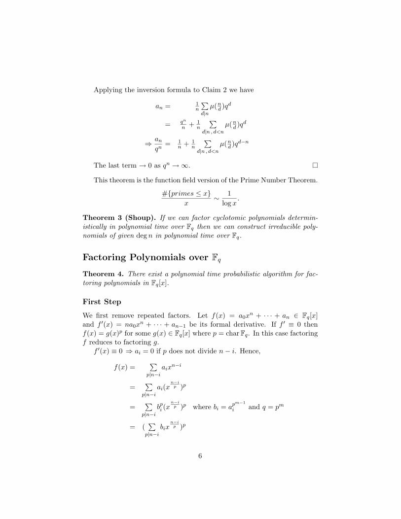
Applying the inversion formula to Claim 2 we have

an = 1n

∑d|n

µ(nd )qd

= qn

n + 1n

∑d|n , d<n

µ(nd )qd

⇒ an

qn= 1

n + 1n

∑d|n , d<n

µ(nd )qd−n

The last term → 0 as qn →∞.

This theorem is the function field version of the Prime Number Theorem.

#{primes ≤ x}x

∼ 1log x

.

Theorem 3 (Shoup). If we can factor cyclotomic polynomials determin-istically in polynomial time over Fq then we can construct irreducible poly-nomials of given deg n in polynomial time over Fq.

Factoring Polynomials over Fq

Theorem 4. There exist a polynomial time probabilistic algorithm for fac-toring polynomials in Fq[x].

First Step

We first remove repeated factors. Let f(x) = a0xn + · · · + an ∈ Fq[x]

and f ′(x) = na0xn + · · · + an−1 be its formal derivative. If f ′ ≡ 0 then

f(x) = g(x)p for some g(x) ∈ Fq[x] where p = char Fq. In this case factoringf reduces to factoring g.

f ′(x) ≡ 0 ⇒ ai = 0 if p does not divide n− i. Hence,

f(x) =∑

p|n−i

aixn−i

=∑

p|n−i

ai(xn−i

p )p

=∑

p|n−i

bpi (x

n−ip )p where bi = apm−1

i and q = pm

= (∑

p|n−i

bixn−i

p )p

6

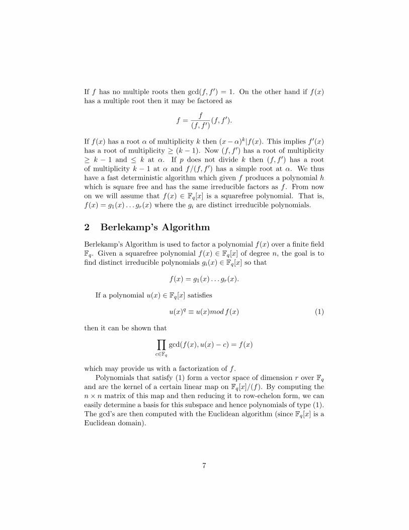
If f has no multiple roots then gcd(f, f ′) = 1. On the other hand if f(x)has a multiple root then it may be factored as

f =f

(f, f ′)(f, f ′).

If f(x) has a root α of multiplicity k then (x−α)k|f(x). This implies f ′(x)has a root of multiplicity ≥ (k − 1). Now (f, f ′) has a root of multiplicity≥ k − 1 and ≤ k at α. If p does not divide k then (f, f ′) has a rootof multiplicity k − 1 at α and f/(f, f ′) has a simple root at α. We thushave a fast deterministic algorithm which given f produces a polynomial hwhich is square free and has the same irreducible factors as f . From nowon we will assume that f(x) ∈ Fq[x] is a squarefree polynomial. That is,f(x) = g1(x) . . . gr(x) where the gi are distinct irreducible polynomials.

2 Berlekamp’s Algorithm

Berlekamp’s Algorithm is used to factor a polynomial f(x) over a finite fieldFq. Given a squarefree polynomial f(x) ∈ Fq[x] of degree n, the goal is tofind distinct irreducible polynomials gi(x) ∈ Fq[x] so that

f(x) = g1(x) . . . gr(x).

If a polynomial u(x) ∈ Fq[x] satisfies

u(x)q ≡ u(x)mod f(x) (1)

then it can be shown that∏c∈Fq

gcd(f(x), u(x)− c) = f(x)

which may provide us with a factorization of f .Polynomials that satisfy (1) form a vector space of dimension r over Fq

and are the kernel of a certain linear map on Fq[x]/(f). By computing then× n matrix of this map and then reducing it to row-echelon form, we caneasily determine a basis for this subspace and hence polynomials of type (1).The gcd’s are then computed with the Euclidean algorithm (since Fq[x] is aEuclidean domain).

7

2.1 Details

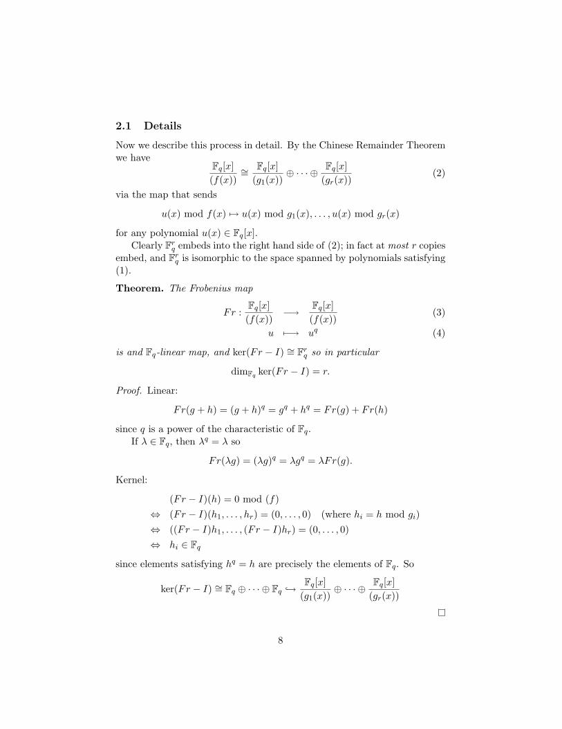
Now we describe this process in detail. By the Chinese Remainder Theoremwe have

Fq[x](f(x))

∼=Fq[x]

(g1(x))⊕ · · · ⊕ Fq[x]

(gr(x))(2)

via the map that sends

u(x) mod f(x) 7→ u(x) mod g1(x), . . . , u(x) mod gr(x)

for any polynomial u(x) ∈ Fq[x].Clearly Fr

q embeds into the right hand side of (2); in fact at most r copiesembed, and Fr

q is isomorphic to the space spanned by polynomials satisfying(1).

Theorem. The Frobenius map

Fr :Fq[x](f(x))

−→ Fq[x](f(x))

(3)

u 7−→ uq (4)

is and Fq-linear map, and ker(Fr − I) ∼= Frq so in particular

dimFq ker(Fr − I) = r.

Proof. Linear:

Fr(g + h) = (g + h)q = gq + hq = Fr(g) + Fr(h)

since q is a power of the characteristic of Fq.If λ ∈ Fq, then λq = λ so

Fr(λg) = (λg)q = λgq = λFr(g).

Kernel:

(Fr − I)(h) = 0 mod (f)⇔ (Fr − I)(h1, . . . , hr) = (0, . . . , 0) (where hi = h mod gi)⇔ ((Fr − I)h1, . . . , (Fr − I)hr) = (0, . . . , 0)⇔ hi ∈ Fq

since elements satisfying hq = h are precisely the elements of Fq. So

ker(Fr − I) ∼= Fq ⊕ · · · ⊕ Fq ↪→ Fq[x](g1(x))

⊕ · · · ⊕ Fq[x](gr(x))

8

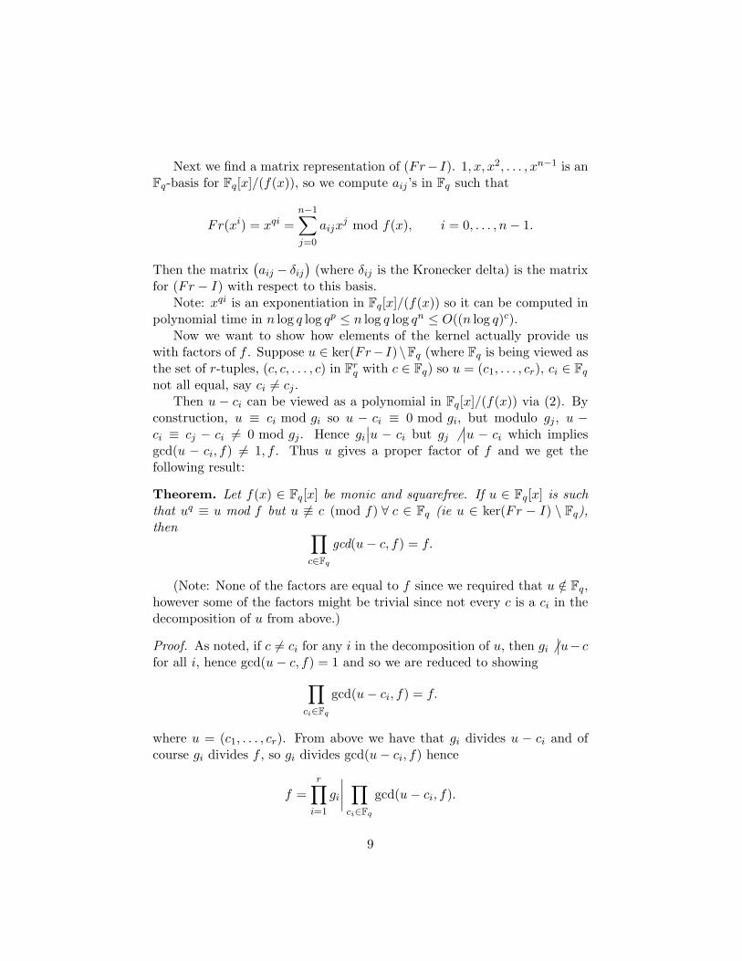
Next we find a matrix representation of (Fr− I). 1, x, x2, . . . , xn−1 is anFq-basis for Fq[x]/(f(x)), so we compute aij ’s in Fq such that

Fr(xi) = xqi =n−1∑j=0

aijxj mod f(x), i = 0, . . . , n− 1.

Then the matrix(aij − δij

)(where δij is the Kronecker delta) is the matrix

for (Fr − I) with respect to this basis.Note: xqi is an exponentiation in Fq[x]/(f(x)) so it can be computed in

polynomial time in n log q log qp ≤ n log q log qn ≤ O((n log q)c).Now we want to show how elements of the kernel actually provide us

with factors of f . Suppose u ∈ ker(Fr− I)\Fq (where Fq is being viewed asthe set of r-tuples, (c, c, . . . , c) in Fr

q with c ∈ Fq) so u = (c1, . . . , cr), ci ∈ Fq

not all equal, say ci 6= cj .Then u − ci can be viewed as a polynomial in Fq[x]/(f(x)) via (2). By

construction, u ≡ ci mod gi so u − ci ≡ 0 mod gi, but modulo gj , u −ci ≡ cj − ci 6= 0 mod gj . Hence gi

∣∣u − ci but gj 6∣∣u − ci which implies

gcd(u − ci, f) 6= 1, f . Thus u gives a proper factor of f and we get thefollowing result:

Theorem. Let f(x) ∈ Fq[x] be monic and squarefree. If u ∈ Fq[x] is suchthat uq ≡ u mod f but u 6≡ c (mod f) ∀ c ∈ Fq (ie u ∈ ker(Fr − I) \ Fq),then ∏

c∈Fq

gcd(u− c, f) = f.

(Note: None of the factors are equal to f since we required that u /∈ Fq,however some of the factors might be trivial since not every c is a ci in thedecomposition of u from above.)

Proof. As noted, if c 6= ci for any i in the decomposition of u, then gi 6∣∣u− c

for all i, hence gcd(u− c, f) = 1 and so we are reduced to showing∏ci∈Fq

gcd(u− ci, f) = f.

where u = (c1, . . . , cr). From above we have that gi divides u − ci and ofcourse gi divides f , so gi divides gcd(u− ci, f) hence

f =r∏

i=1

gi

∣∣∣∣ ∏ci∈Fq

gcd(u− ci, f).

9

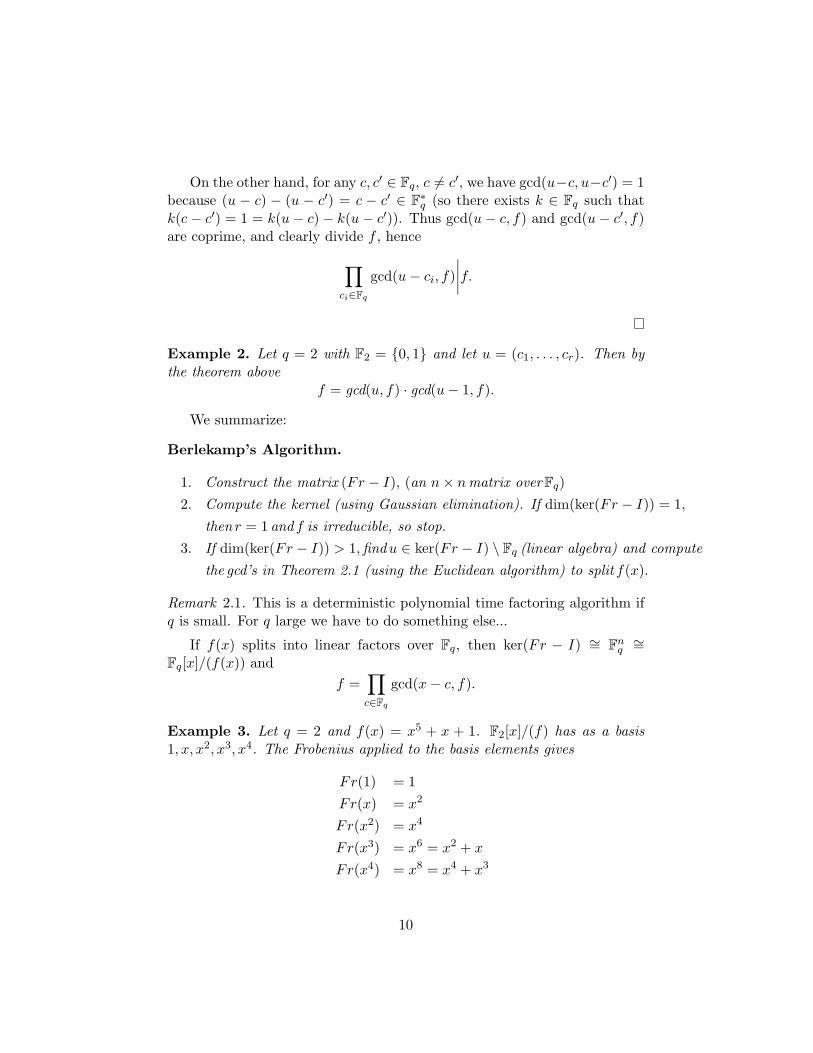
On the other hand, for any c, c′ ∈ Fq, c 6= c′, we have gcd(u−c, u−c′) = 1because (u − c) − (u − c′) = c − c′ ∈ F∗q (so there exists k ∈ Fq such thatk(c− c′) = 1 = k(u− c)− k(u− c′)). Thus gcd(u− c, f) and gcd(u− c′, f)are coprime, and clearly divide f , hence∏

ci∈Fq

gcd(u− ci, f)∣∣∣∣f.

Example 2. Let q = 2 with F2 = {0, 1} and let u = (c1, . . . , cr). Then bythe theorem above

f = gcd(u, f) · gcd(u− 1, f).

We summarize:

Berlekamp’s Algorithm.

1. Construct the matrix (Fr − I), (an n× nmatrix over Fq)2. Compute the kernel (using Gaussian elimination). If dim(ker(Fr − I)) = 1,

then r = 1 and f is irreducible, so stop.3. If dim(ker(Fr − I)) > 1,findu ∈ ker(Fr − I) \ Fq (linear algebra) and compute

the gcd’s in Theorem 2.1 (using the Euclidean algorithm) to split f(x).

Remark 2.1. This is a deterministic polynomial time factoring algorithm ifq is small. For q large we have to do something else...

If f(x) splits into linear factors over Fq, then ker(Fr − I) ∼= Fnq∼=

Fq[x]/(f(x)) andf =

∏c∈Fq

gcd(x− c, f).

Example 3. Let q = 2 and f(x) = x5 + x + 1. F2[x]/(f) has as a basis1, x, x2, x3, x4. The Frobenius applied to the basis elements gives

Fr(1) = 1Fr(x) = x2

Fr(x2) = x4

Fr(x3) = x6 = x2 + x

Fr(x4) = x8 = x4 + x3

10

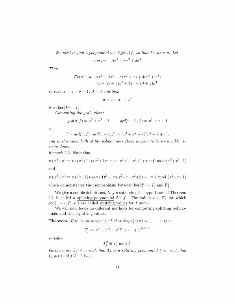
We need to find a polynomial u ∈ F2[x]/(f) so that Fr(u) = u. Let

u = αx + βx2 + γx3 + δx4

Then

Fr(u) = αx2 + βx4 + γ(x2 + x) + δ(x4 + x3)γx + (α + γ)x2 + δx3 + (β + γ)x4

so take α = γ = δ = 1, β = 0 and then

u = x + x3 + x4

is in ker(Fr − I).Computing the gcd’s gives:

gcd(u, f) = x3 + x2 + 1, gcd(u + 1, f) = x2 + x + 1

sof = gcd(u, f) · gcd(u + 1, f) = (x3 + x2 + 1)(x2 + x + 1),

and in this case, both of the polynomials above happen to be irreducible, sowe’re done.Remark 2.2. Note that

x+x3+x4 ≡ x+(x2+1)+(x2+1)x ≡ x+x2+1+x2+1+x ≡ 0 mod (x3+x2+1)

and

x+x3+x4 ≡ x+(x+1)x+(x+1)2 = x+x2+x+x2+2x+1 ≡ 1 mod (x2+x+1)

which demonstrates the isomorphism between ker(Fr − I) and F22.

We give a couple definitions, Any u satisfying the hypotheses of Theorem2.1 is called a splitting polynomial for f . The values c ∈ Fq for whichgcd(u− c, f) 6= 1 are called splitting values for f and u.

We will now focus on different methods for computing splitting polyno-mials and their splitting values.

Theorem. If m is an integer such that deg gi

∣∣m∀ i = 1, . . . , r then

Tj := xj + xjq + xjq2+ · · ·+ xjqm−1

satisfiesT q

j ≡ Tj mod f.

Furthermore ∃ j ≤ n such that Tj is a splitting polynomial (i.e. such thatTj 6≡ c mod f ∀ c ∈ Fq).

11

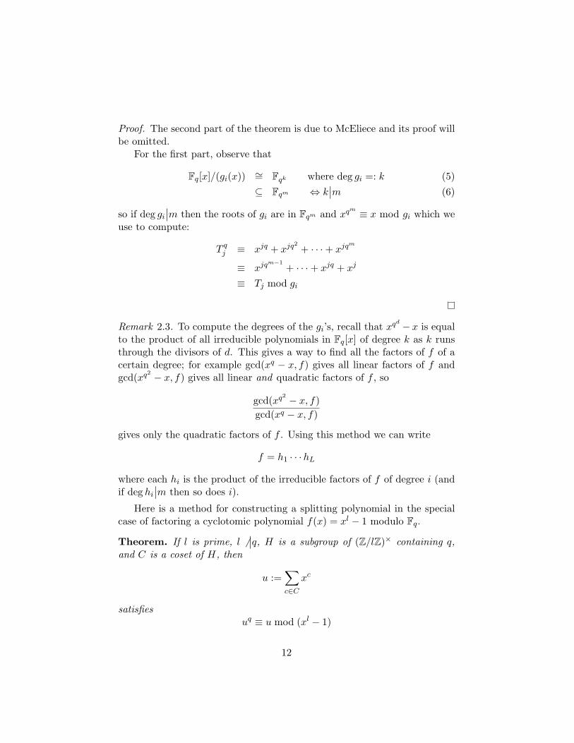
Proof. The second part of the theorem is due to McEliece and its proof willbe omitted.

For the first part, observe that

Fq[x]/(gi(x)) ∼= Fqk where deg gi =: k (5)⊆ Fqm ⇔ k

∣∣m (6)

so if deg gi

∣∣m then the roots of gi are in Fqm and xqm ≡ x mod gi which weuse to compute:

T qj ≡ xjq + xjq2

+ · · ·+ xjqm

≡ xjqm−1+ · · ·+ xjq + xj

≡ Tj mod gi

Remark 2.3. To compute the degrees of the gi’s, recall that xqd − x is equalto the product of all irreducible polynomials in Fq[x] of degree k as k runsthrough the divisors of d. This gives a way to find all the factors of f of acertain degree; for example gcd(xq − x, f) gives all linear factors of f andgcd(xq2 − x, f) gives all linear and quadratic factors of f , so

gcd(xq2 − x, f)gcd(xq − x, f)

gives only the quadratic factors of f . Using this method we can write

f = h1 · · ·hL

where each hi is the product of the irreducible factors of f of degree i (andif deg hi

∣∣m then so does i).

Here is a method for constructing a splitting polynomial in the specialcase of factoring a cyclotomic polynomial f(x) = xl − 1 modulo Fq.

Theorem. If l is prime, l 6∣∣q, H is a subgroup of (Z/lZ)× containing q,

and C is a coset of H, then

u :=∑c∈C

xc

satisfiesuq ≡ u mod (xl − 1)

12

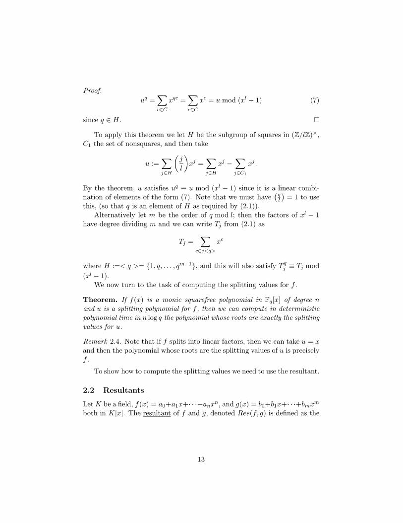
Proof.uq =

∑c∈C

xqc =∑c∈C

xc = u mod (xl − 1) (7)

since q ∈ H.

To apply this theorem we let H be the subgroup of squares in (Z/lZ)×,C1 the set of nonsquares, and then take

u :=∑j∈H

(j

l

)xj =

∑j∈H

xj −∑j∈C1

xj .

By the theorem, u satisfies uq ≡ u mod (xl − 1) since it is a linear combi-nation of elements of the form (7). Note that we must have

( ql

)= 1 to use

this, (so that q is an element of H as required by (2.1)).Alternatively let m be the order of q mod l; then the factors of xl − 1

have degree dividing m and we can write Tj from (2.1) as

Tj =∑

c∈j<q>

xc

where H :=< q >= {1, q, . . . , qm−1}, and this will also satisfy T qj ≡ Tj mod

(xl − 1).We now turn to the task of computing the splitting values for f .

Theorem. If f(x) is a monic squarefree polynomial in Fq[x] of degree nand u is a splitting polynomial for f , then we can compute in deterministicpolynomial time in n log q the polynomial whose roots are exactly the splittingvalues for u.

Remark 2.4. Note that if f splits into linear factors, then we can take u = xand then the polynomial whose roots are the splitting values of u is preciselyf .

To show how to compute the splitting values we need to use the resultant.

2.2 Resultants

Let K be a field, f(x) = a0+a1x+· · ·+anxn, and g(x) = b0+b1x+· · ·+bmxm

both in K[x]. The resultant of f and g, denoted Res(f, g) is defined as the

13

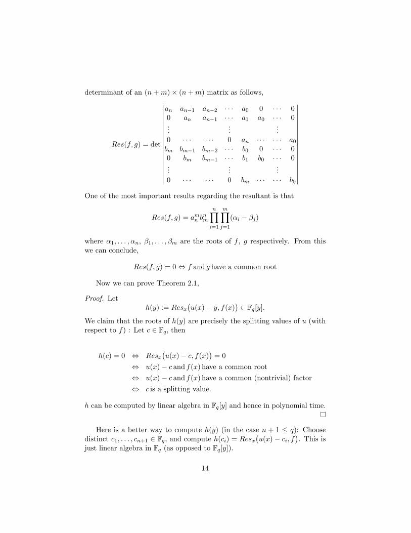
determinant of an (n + m)× (n + m) matrix as follows,

Res(f, g) = det

∣∣∣∣∣∣∣∣∣∣∣∣∣∣∣∣∣∣

an an−1 an−2 · · · a0 0 · · · 00 an an−1 · · · a1 a0 · · · 0...

......

0 · · · · · · 0 an · · · · · · a0

bm bm−1 bm−2 · · · b0 0 · · · 00 bm bm−1 · · · b1 b0 · · · 0...

......

0 · · · · · · 0 bm · · · · · · b0

∣∣∣∣∣∣∣∣∣∣∣∣∣∣∣∣∣∣One of the most important results regarding the resultant is that

Res(f, g) = amn bn

m

n∏i=1

m∏j=1

(αi − βj)

where α1, . . . , αn, β1, . . . , βm are the roots of f , g respectively. From thiswe can conclude,

Res(f, g) = 0⇔ f and g have a common root

Now we can prove Theorem 2.1,

Proof. Leth(y) := Resx

(u(x)− y, f(x)

)∈ Fq[y].

We claim that the roots of h(y) are precisely the splitting values of u (withrespect to f) : Let c ∈ Fq, then

h(c) = 0 ⇔ Resx

(u(x)− c, f(x)

)= 0

⇔ u(x)− c and f(x) have a common root⇔ u(x)− c and f(x) have a common (nontrivial) factor⇔ c is a splitting value.

h can be computed by linear algebra in Fq[y] and hence in polynomial time.

Here is a better way to compute h(y) (in the case n + 1 ≤ q): Choosedistinct c1, . . . , cn+1 ∈ Fq, and compute h(ci) = Resx

(u(x)− ci, f

). This is

just linear algebra in Fq (as opposed to Fq[y]).

14

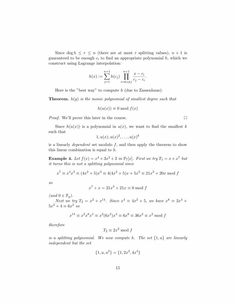
Since deg h ≤ r ≤ n (there are at most r splitting values), n + 1 isguaranteed to be enough ci to find an appropriate polynomial h, which weconstruct using Lagrange interpolation:

h(x) :=n+1∑j=1

h(cj)n+1∏

i=0,i6=j

x− ci

cj − ci.

Here is the ”best way” to compute h (due to Zassenhaus):

Theorem. h(y) is the monic polynomial of smallest degree such that

h(u(x)) ≡ 0 mod f(x)

Proof. We’ll prove this later in the course.

Since h(u(x)) is a polynomial in u(x), we want to find the smallest ksuch that

1, u(x), u(x)2, . . . , u(x)k

is a linearly dependent set modulo f , and then apply the theorem to showthis linear combination is equal to h.

Example 4. Let f(x) = x4 +3x2 +2 in F7[x]. First we try T1 = x+x7 butit turns this is not a splitting polynomial since

x7 ≡ x4x3 ≡ (4x2 + 5)x3 ≡ 4(4x2 + 5)x + 5x3 ≡ 21x3 + 20x mod f

sox7 + x = 21x3 + 21x ≡ 0 mod f

(and 0 ∈ Fq).Next we try T2 = x2 + x14. Since x4 ≡ 4x2 + 5, we have x8 ≡ 2x4 +

5x2 + 4 ≡ 6x2 so

x14 ≡ x2x8x4 ≡ x2(6x2)x4 ≡ 6x8 ≡ 36x2 ≡ x2 mod f

thereforeT2 ≡ 2x2 mod f

is a splitting polynomial. We now compute h. The set {1, u} are linearlyindependent but the set

{1, u, u2} = {1, 2x2, 4x4}

15

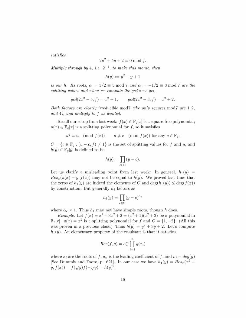
satisfies2u2 + 5u + 2 ≡ 0 mod f.

Multiply through by 4, i.e. 2−1, to make this monic, then

h(y) := y2 − y + 1

is our h. Its roots, c1 = 3/2 ≡ 5 mod 7 and c2 = −1/2 ≡ 3 mod 7 are thesplitting values and when we compute the gcd’s we get,

gcd(2x2 − 5, f) = x2 + 1, gcd(2x2 − 3, f) = x2 + 2.

Both factors are clearly irreducible mod7 (the only squares mod7 are 1, 2,and 4), and multiply to f as wanted.

Recall our setup from last week: f(x) ∈ Fq[x] is a square-free polynomial;u(x) ∈ Fq[x] is a splitting polynomial for f , so it satisfies

uq ≡ u (mod f(x)) u 6≡ c (mod f(x)) for any c ∈ Fq;

C = {c ∈ Fq : (u − c, f) 6= 1} is the set of splitting values for f and u; andh(y) ∈ Fq[y] is defined to be

h(y) =∏c∈C

(y − c).

Let us clarify a misleading point from last week: In general, h1(y) =Resx(u(x) − y, f(x)) may not be equal to h(y). We proved last time thatthe zeros of h1(y) are indeed the elements of C and deg(h1(y)) ≤ deg(f(x))by construction. But generally h1 factors as

h1(y) =∏c∈C

(y − c)αc

where αc ≥ 1. Thus h1 may not have simple roots, though h does.Example. Let f(x) = x4 + 3x2 + 2 = (x2 + 1)(x2 + 2) be a polynomial in

F7[x]. u(x) = x2 is a splitting polynomial for f and C = {1,−2}. (All thiswas proven in a previous class.) Thus h(y) = y2 + 3y + 2. Let’s computeh1(y). An elementary property of the resultant is that it satisfies

Res(f, g) = amn

n∏i=1

g(xi)

where xi are the roots of f , an is the leading coefficient of f , and m = deg(g)[See Dummit and Foote, p. 621]. In our case we have h1(y) = Resx(x2 −y, f(x)) = f(

√y)f(−√y) = h(y)2.

16

Theorem. h(y) is the monic polynomial of smallest degree such that f(x)divides h(u(x)).

Proof. Observe that I = {g(y) ∈ Fq[x] : f(x)|g(u(x))} is an ideal in Fq[x],which is a prinicipal ideal domain and hence I is generated by a singleelement (of minimal degree). Our claim is equivalent to the claim thatI = (h). First observe that h ∈ I: recall that f = g1 · · · gr where each gi

is irreducible and that u ≡ ci (mod gi) for some ci ∈ Fq. (For this lastclaim, recall uq ≡ u (mod f), so uq ≡ u (mod gi) for all i. Since the gi’s areirreducible, Fq[x]/(gi) is a finite field containing a copy of Fq as the solutionsof xq ≡ x (mod gi). Thus u ≡ ci (mod gi) for some ci ∈ Fq ⊆ Fq[x]/(gi).)Thus gi divides u − ci and hence also

∏c∈Fq

(u − c) = h(u). Thus every gi

divides h(u), so f does as well.Now assume I = (k) for some k ∈ Fq[y], k 6= h. Since h ∈ I, we know k

divides h, sok(y) =

∏c∈C′

(y − c)

for C ′ ( C. So there exists a ci ∈ C such that ci /∈ C ′. Recall that weknow u ≡ ci (mod gi) for some i. We claim for this fixed i, gi does notdivide k(u). Assume this is not true, so gi divides

∏c∈C′(u − c). But gi is

irreducible and hence a prime in Fq[x], so gi divides u−c for some c ∈ C ′, sou ≡ c (mod gi), but u ≡ ci (mod gi). Thus c = ci, but this contradicts thefact that ci /∈ C ′. Thus for some i, gi does not divide k(u), hence neitherdoes f , so k /∈ I, a contradiction. Hence k must be h, so I = (h).

Problem: Given a square-free f(x) ∈ Fq[x] that splits completely in Fq

(i.e. f(x) divides xq − x), find the (distinct) roots of f(x).We have a probabilistic algorithm that is quite fast in practice due to

Legendre. The idea is to split up Fq into two disjoint halves and hope thatthis will induce a splitting of f . After at most deg f successful splits, wewill have found its roots. Here is the procedure:

Algorithm: Suppose first that q is odd. Observe that

xq − x = x(x(q−1)/2 − 1)(x(q−1)/2 + 1).

The last two factors on the right distinguish the squares from the non-squares in Fq, respectively, and the first factor distinguishes 0. With this inmind, pick a b ∈ Fq at random and consider

f(x) = (f(x), x− b) · (f(x), (x− b)(q−1)/2 − 1) · (f(x), (x− b)(q−1)/2 + 1).

17

If this is a non-trivial splitting of f , recurse over these other factors bychoosing different b’s. If not, choose a different b and try again.

Now suppose q is even, so say q = 2m. Let S(x) = x + x2 + · · ·+ x2m−1.

Observe S(x)(S(x)+1) = xq−x. So for any a ∈ Fq, S(a) = TrFq/F2(a) ∈ F2.

Again, select a b ∈ Fq at random and consider

f(x) = (f(x), S(bx)) · (f(x), S(bx) + 1).

If this is a non-trivial splitting of f , again recurse over these factors withnew b’s. If not, choose a different b and try again.Remark 2.5. (q odd.) Computing (x− b)(q−1)/2 using modular exponentia-tion is fast, as is computing the gcd’s. Hence the only difficulty is finding asatisfactory b. So how often do we have a “bad” b, i.e. a b for which we get anon-trivial splitting of f? Suppose f(x) =

∏ni=1(x− ci). Then f(x) divides

(x− b)(q−1)/2− 1 if and only if x− ci divides (x− b)(q−1)/2− 1 for all i if andonly if (ci− b)(q−1)/2 = 1 for all i. Equivalently, ci− b is a square for every i.We will prove later that the probability of this event is approximately 2−n

where n is the degree of f .Remark 2.6. (q even.) We will show below that picking a “bad” b in thiscase also has small probability.

We have the following theorems:

Theorem. For c1, . . . , cn ∈ Fq distinct, q odd,

#{b ∈ Fq : b− ci is a square for all i} =q

2n+ O(n

√q)

Proof. Consider the system of equations

x− ci = y2i (8)

for i = 1, . . . , n in the variables x, y1, . . . , yn. Any b for which b − ci is anon-zero square in Fq for all i gives rise to solutions x = b, yi = ±

√b− ci.

Thus we see that every such b 6= ci,∀i yields 2n solutions to the system(8). Our claim will follow if and only if (8) has q + O(2nn

√q) solutions

in Fq. Observe that (8) defines an affine algebraic curve X over Fq. Wehave the map φ : X → A1 given by (x, y1, . . . , yn) 7→ x. This extends to arational map X → P1, where X is the projective closure of X. (In fact thisis a (2, . . . , 2) Galois cover of P1.) The genus of (the normalization of) Xis g = 2n−2(n − 3) + 1, which can be calculated using Hurwitz’s formula.Recall the Weil bound:

18

Lemma. If X is a smooth irreducbile projective curve over Fq of genus g,then

|#X(Fq)− (q + 1)| ≤ 2g√

q.

Thus the estimate q + O(2nn√

q) for the number points on X is just theWeil bound. This completes the proof.

Theorem. For c1, . . . , cn ∈ Fq distinct, q even,

#{b ∈ Fq : S(bci) = 0 for all i} =q

2k= 2m−k

where k is the dimension of the F2-vector space spanned by c1, . . . , cn insideFq.

Proof. Observe that S is F2-linear: S(x + y) = S(x) + S(y) since we are incharacteristic 2. Let V = {b ∈ Fq : S(bci) = 0 for all i} be the F2-subspaceof Fq. We want to show that dimF2(V ) = m − k. We recall the followinglemma from field theory:

Lemma. If L/K is a finite separable extension of fields then the map L×L→ K given by (x, y) 7→ TrL/K(xy) is a non-degenerate bilinear pairing ofK-vector spaces, where TrL/K is the trace of L/K.

Now TrFq/F2(x) = S(x) for all x ∈ Fq. Observe that V is the orthogonal

complement to c1, . . . , cn with respect to the trace pairing since S(bci) = 0implies b is orthogonal to ci with respect to this pairing. Thus dimF2(V ) =dimF2(Fq) − dimF2(V

⊥) = m − k where k = dimF2(span(c1, . . . , cn)). Thiscompletes the proof.Remark 2.7. (q even.) Recall that we have

f =n∏

i=1

(x− ci)

and we also have

f(x) = (f(x), S(bx))(f(x), S(bx) + 1)).

We have already discussed the “bad” b’s arising from the first factor. Forthe second factor, consider the set V1 : {b ∈ Fq : S(bci) = 1 for all i}. Nextobserve that if there exists a b0 ∈ Fq such that S(bci) = 1 for all i, thenV1 = b0 + V since S is F2-linear, so V1 is just a translation of V by b0. Insuch a case, we see that #V1 = #V . A priori though, there may exist no

19

such b0. For observe that V ∩ V1 = ∅, thus if V = Fq, V1 = ∅ and we willhave no such b0.

Now writing f as

f(x) = (f(x), S(bx))(f(x), S(bx) + 1)

=∏

ci∈Fq ,S(bci)=0

(x− ci)∏

ci∈Fq ,S(bci)=1

(x− ci),

we see this is a (non-trivial) splitting of f if and only if b 6∈ V ∪V1 (otherwiseone of the products contains all of the ci’s, and hence is f). Now #(V ∪V1) =#V +#V1 ≤ 2#V = q/2k−1 ≤ q/2 if k ≥ 2. So if k is at least 2, then at leasthalf of the b’s are “good.” For k = 0, we see that {c1, . . . , cn} = {0} sincethey span just 0, which corresponds to the polynomial f(x) = x, whichis already factored. For k = 1, we have that all of the ci’s are F2-linearcombinations of one c ∈ {c1, . . . , cn}, c 6= 0. This means f divides x(x− c),hence is a quadratic which we can factor easily. These becomes trivial cases,which we check for, and otherwise we use the above algorithm.

Another significant improvement can be made though. We can make thisprobabilistic algorithm into a deterministic one via the following proposition:

Proposition 5. Let b1, . . . , bm be a basis for Fq over F2. Then there exists aj such that bj 6∈ V ∪ V1 so long as m ≥ 2.

In fact, thinking of Fq as F2/(g(x)) where g(x) ∈ F2[x] is an irreduciblepolynomial of degree m, we have the natural basis {1, x, x2, . . . , xm−1} where· is reduction modulo g.

Proof of Proposition. We argue by contradiction: suppose every bj is anelement of V ∪ V1. Then for all j, S(bjci) are all equal. In particularS(bjc1) = S(bjc2) for all j. So S(bj(c1 − c2)) = 0 for all j by linearity of S.So c1 − c2 is orthogonal to every basis element. But S is a non-degeneratebilinear pairing, so c1 − c2 = 0, contradicting the assumption that f hasdistinct roots.

Thus for q even, we have a deterministic polynomial time factoring al-gorithm by picking a b from a basis of Fq/F2 instead of a random b.

Remark 2.8. (q odd.) A similar strategy works for q = pm, p a small oddprime. Define

S(x) = x + xp + · · ·xpm−1,

20

which is just TrFq/Fp(x). Then

f(x) =p−1∏j=0

(f(x), S(bx)− j).

We want to find a b such that this is a (non-trivial) splitting. As before,there always exists such a b within a basis of Fq/Fp. This then gives us adeterministic polynomial time algorithm for factoring f in Fq where char(Fq)is small. This algorithm has running time O((np log q)c).

Thus we have deterministic polynomial time algorithms for even q andodd q’s with small characteristic (with respect to n log q). This leaves onlyFq with large characteristic, such as Fp with p large. We will tackle this nextweek.

Problem. Given a ∈ Fq (with q odd) such that a is a square; find xsuch that x2 = a. This is equivalent to factoring the polynomial x2−a. Notethat a ∈ F∗q is a square if and only if a

q−12 = 1.

The general techniques for polynomial solving give probabilistic poly-nomial time algorithms. For example, we can take the greatest commondivisor

(x2 − a, (x− b)q−12 − 1)

for random b. (See last lecture).Today we will see some algorithms that are specific for square roots and

outperform the general polynomial solving algorithms in some situations.

3 An algorithm

Let q ≡ 3 (mod 4). If aq−12 = 1 then a

q−12 a = a but a

q−12 a = a

q+12 = (a

q+14 )2.

Hence x = ±aq+14 are the square roots of a in Fq.

Note that this is a consequence of a fact that holds for every group ofodd cardinality: |G| = m ≡ 1 (mod 2) ⇒ (g

m+12 )2 = g ∀ g ∈ G. Now q ≡

3 (mod 4) ⇒#[(F∗q)2] = q−1

2 is odd.This is a nice way to take square roots in groups of odd order. We can

try to generalize this idea. Write q − 1 = 2rm with m odd.Since F∗q is a cyclic group, it has a unique subgroup of order m, let’s call

it G :

G = {x ∈ F∗q | xm = 1}.

21

Then the following sequence is exact, and |F∗q/G| = 2r :

0→ G ↪→ F∗q → F∗q/G→ 0

|F∗q/G| = 2r and F∗q ' G× F∗q/G.Suppose c ∈ F∗q is not a square. Then using c we will have a deterministic

algorithm for taking square roots in F∗q which is good if r is small. We discusshow to find c below.

Given a ∈ F∗q set e0 = 0, and for i = 1, ..., r do: if (ac−ei−1)q−1

2i−1 6= 1 putei = ei−1+2i−1, otherwise, ei = ei−1. We will show below that ac−er ∈ G,i.e.(ac−er)m = 1.

Claim. er even ⇒ (ac−er)m+1

2 cer2 is a square root of a.

Proof. Since m is odd and er is even, all the exponents in the expressionare integers. Now let’s take the square:

[(ac−er)m+1

2 cer2 ]2 =

(ac−er)m+1cer =(ac−er)m(ac−er)cer =a(c−ercer) = a

Claim. For all i = 0, . . . , r (ac−ei)q−1

2i = 1.Proof. By induction.i = 0 : (ac−e0)q−1 = 1 automatically. (Nothing to be checked).

1 ≤ i ≤ r − 1 : (ac−ei−1)q−1

2i−1 = 1 by our inductive hypothesis. Takingsquare roots on both sides we obtain:

(ac−ei−1)q−1

2i = ±1,

so there are two cases to check.Case 1: = +1. Here ei = ei−1, so (ac−ei)

q−1

2i = 1.

22

Case 2: = −1. Here ei = ei−1 + 2i−1, so

(ac−ei)q−1

2i = (ac−ei−1−2i−1)

q−1

2i

= (ac−ei−1)q−1

2i (c−2i−1)

q−1

2i

= (−1)c−q−12

= (−1) 1−1 (since c is not a square).

= 1

i = r : 1 = (ac−er)q−12r = (ac−er)m, hence ac−er ∈ G.

Note that we get an isomorphism

F∗q/G∼−→ Z/2rZ

a 7→ er

The problem with this algorithm is finding c. If we assume the gen-eralized Riemann hypothesis, for q an odd prime there exists c, 1 ≤ c ≤4(log q)2, with c

q−12 6= 1 (mod q). Note that if for a given q such a c doesn’t

exist, then this would be a counterexample to GRH. Alternatively, we cando a random search for c and each try will have a 0.5 probability of success.

Now suppose a ∈ Fq is a square, and let t ∈ Fq such that f(x) = x2−tx+ais irreducible in Fq[x]. Then for α a root of f, Fq(α) = Fq2 and the normof α is given by the product of α itself and its image under the Frobeniusmorphism, hence:

NFq2/Fq(α) = αq+1 = a.

So αq+12 is a square root of a in Fq2 . Since we are assuming that a has a

square root in Fq, we conclude that αq+12 ∈ Fq.

When is f irreducible? x2−tx+a is irreducible iff t2−4a is not a square.So again we need to find a non square in Fq. We can proceed randomly tofind it or sequentially if we believe GRH.

This algorithm is much faster than the previous one when r, (the 2-adicvaluation of q), is large.

23

4 Schoof’s algorithm

Given a ∈ Z and a prime p, Schoof’s algorithm is a deterministic algorithmto compute a square root of d mod p in polynomial time in |d| log p. It isbased on a method to count rational points on elliptic curves over finitefields.

Let a, b,∈ Fq, with (b, q) = 1 and let’s consider the elliptic curve overthe finite field Fq given by the equation y2 = x3 + ax + b. Thus

E(Fqn) = {(x, y) ∈ Fqn × Fqn | y2 = x3 + ax + b} ∪ {O}

Elliptic curves have a group structure where P + Q + R = O ⇔ P,Q,Rare colinear.

We know #E(Fq) = q + 1− t where |t| ≤ 2√

q.Schoof’s algorithm computes #E(Fq) in polynomial time in log q.Let’s say we compute the square root of d (mod p), d ∈ Z and p prime.

For simplicity, let’s assume d < 0. (Think of 0 < d < p and take d := d− p).We need to find an elliptic curve with complex multiplication 1by Q(

√d)

and reduce it modulo p. We won’t see here how to find such a curve, butit exists. Unfortunately, such a curve is hard to find and that’s why therunning time depends badly on |d|. Assume that E is such a curve.

Let f(x) = x2 − tx + q where #E(Fq) = q + 1− t. Let α be a root of f .

Then{

α.α = qα + α = t

The complex multiplication hypothesis is essentially equivalent to α, α ∈Q(√

d) and this is all we will use of it. Let’s write α = u +√

dv where2u, 2v ∈ Z. Then:{

t = 2u(= α + α)p = u2 − dv2

We will compute u using Schoof, and from that we compute v =√

(u2 − p)/d.Now p = u2− dv2 ⇒ (u

v )2 ≡ d mod p. Hence we would have found a squareroot of d mod p, namely u

v .Example.

d = −1E : y2 = x3 − x (mod p).

E has complex multiplication by Q(i). If p ≡ 1 (mod 4), then the numberof points on the curve is p + 1 − 2u, and u2 + v2 = p. This gives a squareroot of −1 modulo p. As an aside, (p−1

2 )! is also a square root of −1 modulop but is a horrible way to compute it.

1See Silverman’s Advanced topics in the arithmetic of elliptic curves.

24

Example.E : y2 = x3 − 1

E has complex multiplication by Q(√−3).

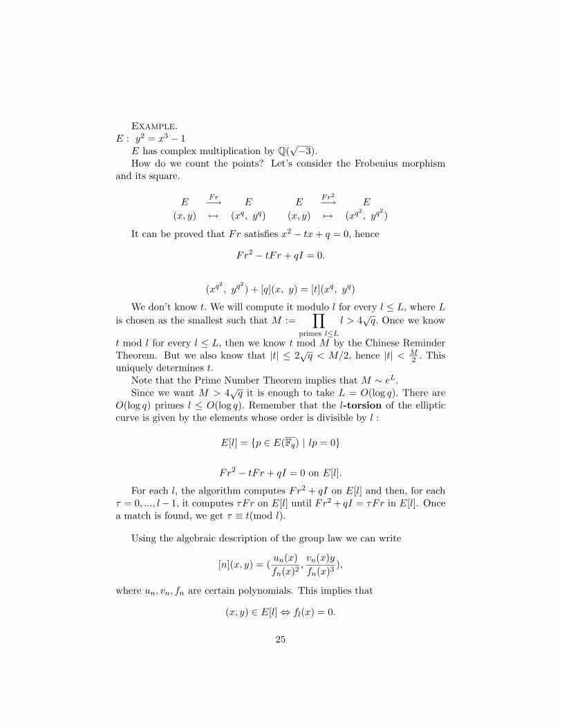
How do we count the points? Let’s consider the Frobenius morphismand its square.

EFr−→ E E

Fr2

−→ E

(x, y) 7→ (xq, yq) (x, y) 7→ (xq2, yq2

)

It can be proved that Fr satisfies x2 − tx + q = 0, hence

Fr2 − tFr + qI = 0.

(xq2, yq2

) + [q](x, y) = [t](xq, yq)

We don’t know t. We will compute it modulo l for every l ≤ L, where L

is chosen as the smallest such that M :=∏

primes l≤L

l > 4√

q. Once we know

t mod l for every l ≤ L, then we know t mod M by the Chinese ReminderTheorem. But we also know that |t| ≤ 2

√q < M/2, hence |t| < M

2 . Thisuniquely determines t.

Note that the Prime Number Theorem implies that M ∼ eL.Since we want M > 4

√q it is enough to take L = O(log q). There are

O(log q) primes l ≤ O(log q). Remember that the l-torsion of the ellipticcurve is given by the elements whose order is divisible by l :

E[l] = {p ∈ E(Fq) | lp = 0}

Fr2 − tFr + qI = 0 on E[l].

For each l, the algorithm computes Fr2 + qI on E[l] and then, for eachτ = 0, ..., l− 1, it computes τFr on E[l] until Fr2 + qI = τFr in E[l]. Oncea match is found, we get τ ≡ t(mod l).

Using the algebraic description of the group law we can write

[n](x, y) = (un(x)fn(x)2

,vn(x)yfn(x)3

),

where un, vn, fn are certain polynomials. This implies that

(x, y) ∈ E[l]⇔ fl(x) = 0.

25

To test the equation (xq2, yq2

) + [q](x, y) = [τ ](xq, yq) in E[l] can betested by computing in Fq[x]/(fl(x)).

For instance, compute un(x)fn(x)2

mod fl where n ≡ q mod l will give the

x coordinate of [q](x, y) in E[l]. Likewise, ( uτ (x)fτ (x)2

)q is the x coordinate of[τ ](xq, yq).

We know that deg fl = l2−12 if l is odd. O(log q

l2−12 ) = O(l2 log q) =

O((log q)3) is required for doing one computation on the ring Fq[x]/(fl(x)).The case l = 2 is a little special but it can be done directly.#E(Fq) = q+1−t and since q is odd, #E(Fq) ≡ t mod 2. Hence #E(Fq)

is even ⇔ (E[2]\{O}) ∩ E(Fq) 6= ∅.Note that the points of odd order come in pairs, whereas E[2]−{O} has

odd cardinality, since its elements correspond to the roots of x3 + ax + b inFq.

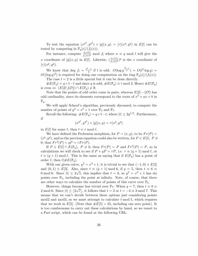
We will apply Schoof’s algorithm, previously discussed, to compute thenumber of points of y2 = x3 + 1 over F5 and F7.

Recall the following: #E(Fq) = q+1−t, where |t| ≤ 2q1/2. Furthermore,if

(xq2, yq2

) + [q](x, y) = τ(xq, yq)

in E[`] for some `, then t ≡ τ mod `.We have defined the Frobenius morphism, for P = (x, y), to be Fr(P ) =

(xq, yq), and so the previous equation could also be written, for P ∈ E[`], P 6=0, that Fr2(P ) + qP = τFr(P ).

If P ∈ E[`] ∩ E(Fq), P 6= 0, then Fr(P ) = P and Fr2(P ) = P , so incalculations we will check to see if P + qP = τP , i.e. τ ≡ (q + 1) mod `, ort ≡ (q + 1) mod `. This is the same as saying that if E(Fq) has a point oforder `, then `|#E(Fq).

With our given curve, y2 = x3 + 1, it is trivial to see that (−1, 0) ∈ E[2]and (0, 1) ∈ E[3]. Also, since t ≡ (q + 1) mod 6, if q = 5, then t ≡ 6 ≡0 mod 6. Since |t| ≤ 2

√5, this implies that t = 0, so y2 = x3 + 1 has six

points over F5, including the point at infinity. Note, of course, that thereare other ways to calculate the number of points of this curve over F5.

However, things become less trivial over F7: When q = 7, then t ≡ 8 ≡2 mod 6. Since |t| ≤ b2

√7c, it follows that t = 2 or t = −4 ≡ 3 mod 7. This

means that we can’t decide between these options just considering pointsmod2 and mod3, so we must attempt to calculate t mod 5, which requiresthat we work in E[5]. (Note that #E[5] = 25, including one zero point). Itis too cumbersome to carry out these calculations by hand, so we resort toa Pari script, which can be found at the following URL.

26

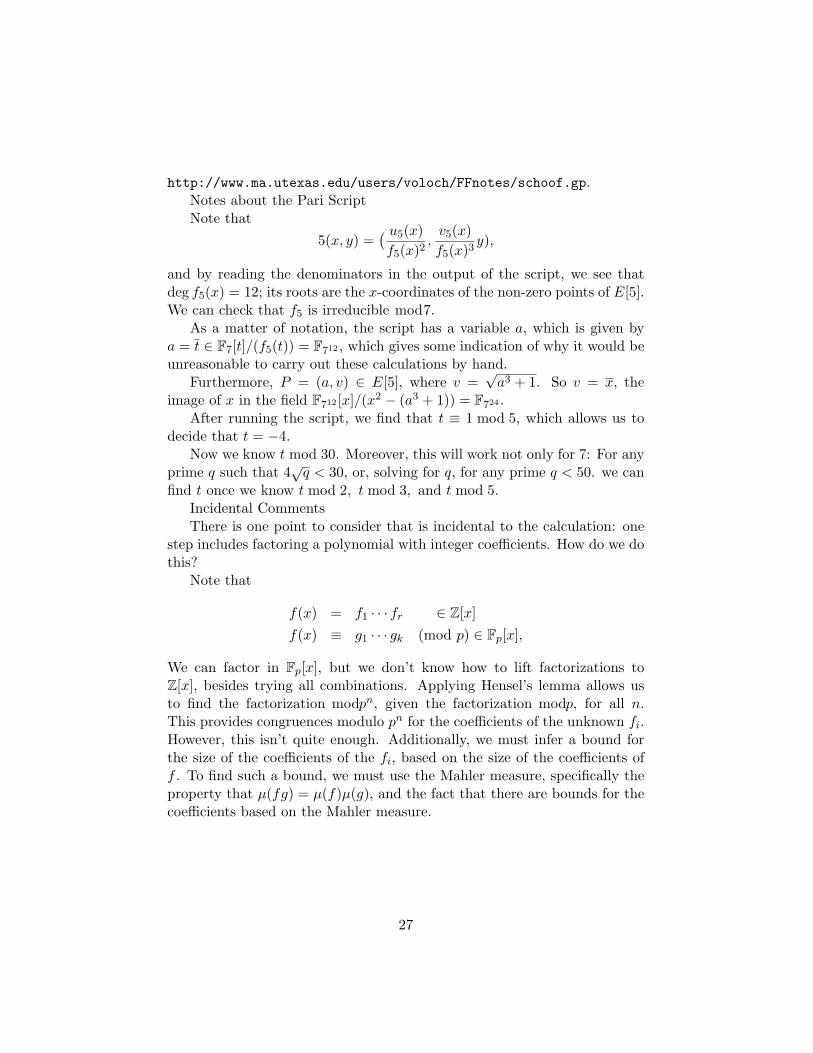
http://www.ma.utexas.edu/users/voloch/FFnotes/schoof.gp.Notes about the Pari ScriptNote that

5(x, y) =( u5(x)f5(x)2

,v5(x)f5(x)3

y),

and by reading the denominators in the output of the script, we see thatdeg f5(x) = 12; its roots are the x-coordinates of the non-zero points of E[5].We can check that f5 is irreducible mod7.

As a matter of notation, the script has a variable a, which is given bya = t ∈ F7[t]/(f5(t)) = F712 , which gives some indication of why it would beunreasonable to carry out these calculations by hand.

Furthermore, P = (a, v) ∈ E[5], where v =√

a3 + 1. So v = x, theimage of x in the field F712 [x]/(x2 − (a3 + 1)) = F724 .

After running the script, we find that t ≡ 1 mod 5, which allows us todecide that t = −4.

Now we know t mod 30. Moreover, this will work not only for 7: For anyprime q such that 4

√q < 30, or, solving for q, for any prime q < 50. we can

find t once we know t mod 2, t mod 3, and t mod 5.Incidental CommentsThere is one point to consider that is incidental to the calculation: one

step includes factoring a polynomial with integer coefficients. How do we dothis?

Note that

f(x) = f1 · · · fr ∈ Z[x]f(x) ≡ g1 · · · gk (mod p) ∈ Fp[x],

We can factor in Fp[x], but we don’t know how to lift factorizations toZ[x], besides trying all combinations. Applying Hensel’s lemma allows usto find the factorization modpn, given the factorization modp, for all n.This provides congruences modulo pn for the coefficients of the unknown fi.However, this isn’t quite enough. Additionally, we must infer a bound forthe size of the coefficients of the fi, based on the size of the coefficients off . To find such a bound, we must use the Mahler measure, specifically theproperty that µ(fg) = µ(f)µ(g), and the fact that there are bounds for thecoefficients based on the Mahler measure.

27

5 Primitive Roots

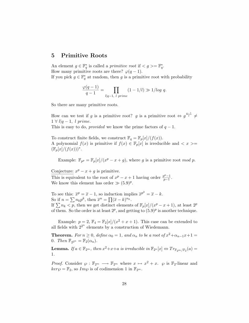
An element g ∈ F∗q is called a primitive root if < g >= F∗q .How many primitive roots are there? ϕ(q − 1).If you pick g ∈ F∗q at random, then g is a primitive root with probability

ϕ(q − 1)q − 1

=∏

l|q−1, l prime

(1− 1/l)� 1/log q.

So there are many primitive roots.

How can we test if g is a primitive root? g is a primitive root ⇔ gq−1

l 6=1 ∀ l|q − 1, l prime.This is easy to do, provided we know the prime factors of q − 1.

To construct finite fields, we construct Fq = Fp[x]/(f(x)).A polynomial f(x) is primitive if f(x) ∈ Fp[x] is irreducible and < x >=(Fp[x]/(f(x)))∗.

Example: Fpp = Fp[x]/(xp − x + g), where g is a primitive root mod p.

Conjecture: xp − x + g is primitive.This is equivalent to the root of xp − x + 1 having order pp−1

p−1 .We know this element has order � (5.9)p.

To see this: xp = x− 1, so induction implies xpk= x− k.

So if n =∑

nkpk, then xn =

∏(x− k)nk .

If∑

nk < p, then we get distinct elements of Fp[x]/(xp − x + 1), at least 2p

of them. So the order is at least 2p, and getting to (5.9)p is another technique.

Example: p = 2, F4 = F2[x]/(x2 + x + 1). This case can be extended toall fields with 22n

elements by a construction of Wiedemann.

Theorem. For n ≥ 0, define α0 = 1, and αn to be a root of x2+αn−1x+1 =0. Then F22n = F2(αn).

Lemma. If a ∈ F2m, then x2+x+a is irreducible in F2n [x]⇔ TrF2m/F2(a) =

1.

Proof. Consider ℘ : F2m −→ F2m where x 7→ x2 + x. ℘ is F2-linear andker℘ = F2, so Im℘ is of codimension 1 in F2m .

28

On the other hand, Im℘ ⊆ ker(TrF2m/F2) because Tr(x2 + x) = Tr(x2) +

Tr(x) = 2Tr(x) = 0 (since x2 and x are conjugates).Since Tr is non-trivial (an algebra fact), we get Im(φ) = ker(Tr).Since quadratics are irreducible when they don’t have roots, we get thelemma.

So now back to the Theorem:

Proof of Theorem. 1α2

n−1(x2 + αn−1x + 1) = ( x

αn−1)2 + ( x

αn−1) + 1

α2n−1

.

We need to prove that Tr( 1α2

n−1) = 1.

We prove this by induction.

Tr(1

α2n−1

) = Tr(1

αn−1) since they are conjugates

= Tr(αn−1 + αn−2) since α2n−1 + αn−2αn−1 + 1 = 0⇒ αn−1 + αn−2 + 1/αn−1 = 0

= TrF22

n−1 /F2(αn−1) + TrF

22n−1 /F2

(αn−2)

Now

TrF22

n−1 /F2(αn−2) = TrF

22n−2 /F2

(TrF22

n−1 /F22

n−2(αn−2)) = 0,

sinceTrF

22n−1 /F

22n−2

(αn−2) = αn−2 + αn−2 = 0

since αn−2 ∈ F22n−2 .

AndTrF

22n−1 /F2

(αn−1) = TrF22

n−2 /F2(TrF

22n−1 /F

22n−2

(αn−1)).

But αn−1 is a root of x2 + αn−2x + 1 over F22n−2 , we get

TrF22

n−1 /F22

n−2(αn−1) = αn−2,

so TrF22

n−1 /F2(αn−1) = 1 by induction.

We will now use the notation q = 22n−1. So Fq2 = Fq(α), where α = αn.

Every element of Fq2 is of the form u + vα, u, v ∈ Fq. Arithmetic is

(u1 + v1α)(u2 + v2α) = (u1u2 + v1v2) + (u1v2 + u2v1 + αn−1v1v2)α.

So to do multiplication in Fq2 , one must do multiplication in Fq, so it’srecursive and can be very efficient in larger fields.

29

Conjecture. αnαn−1 · · ·α1 is a primitive root for F22n for all n.(⇔ αn has order q + 1, i.e. 22n−1

+ 1 ∀ n)

Note that q2−1 = (q−1)(q+1) and that q2−1 = #F∗q2 , q−1 = #F∗q , andq+1 = #{x ∈ F∗q2 |NFq2/Fq

(x) = 1}. On the other hand, α2 +αn−1α+1 = 0,so NFq2/Fq

(α) = 1. So the conjecture is that α is a generator of the subgroupof norm 1 elements of Fq2 .

The conjecture is known for n ≤ 11. The hard part is factoring Fn =22n

+ 1.

Question: Give a lower bound to the order of αn.A good lower bound combined with the partial factorizations of Fn’s mightallow us to check the conjecture for a few more values of n.

6 The Discrete Logarithm Problem

6.1 The Problem

Let G be a cyclic group of order n and g ∈ G a generator, i.e. 〈g〉 = G. TheDiscrete Logarithm Problem is the following. Given h ∈ G, we want to findsome m ∈ Z/nZ such that h = gm.

We currently have no good algorithm for solving the Discrete Log Prob-lem (henceforth called the DLP), but we can reduce the number of stepsit takes from the order n taken by the stupid algorithm of just computingevery power of g until we find the one desired. For example, for a groupof non-prime order n, if we can write n = n1n2 with (n1, n2) = 1, then weknow that G ∼= G1 ×G2, where |Gi| = ni. The group isomorphism is givenby

G ∼= G1 ×G2

x → (xn2 , xn1)yazb ← (y, z), an2 + bn1 = 1.

So the DLP in a group of order n reduces to the DLP on the groups oforder n1 and n2, respectively.

For a general group, the best algorithm for the DLP takes O(√

n) steps.Notice that

√n = e

ln n2 , so the algorithm is exponential in ln n. In F∗q , there

is an algorithm taking O(e(ln n)1/3+ε) steps, known as the “index calculus

30

algorithm”, which is probabilistic in nature. This algorithm performs betterthan exponential time, but still not as good as an ideal polynomial-timealgorithm:

(log n)c < e(log n)α< nc

There is currently no polynomial time algorithm for solving the DLP.

6.2 An Algorithm in O(√

n) (Shank’s “Baby-step/Giant-step”Algorithm)

As above, let G be a cyclic group of order n with generator g. The followingis a deterministic algorithm that, given h ∈ G, computes m such that h = gm

in O(√

n) time.

• (Baby Steps) Compute and store the values 1, g, g2, g3, . . . , gb√

nc

• (Giant Steps) Given h ∈ G, compute hg−ib√

nc for i = 1, 2, . . ., andcompare it with the list 1, g, . . . , gb

√nc, until you find a match. If a

match is found, stop, else proceed to next value of i.

Once you find a match, you’ve just found i, j such that

hg−ib√

nc = gj =⇒ h = gib√

nc+j

Theorem. There is a match with 0 < i ≤ b√

nc + 1. Therefore, the algo-rithm above stops in O(

√n) steps.

Proof. Choose h ∈ G. Then since G is cyclic with generator g, h = gm forsome m. Use the division algorithm to write

m = ib√

nc+ j, 0 ≤ j ≤ b√

nc − 1

Then we have

i =m− j

b√

nc≤ m

b√

nc≤ n− 1b√

nc≤ n− 1√

n− 1=√

n + 1

and it follows that i ≤ b√

nc+ 1.

31

6.3 The Index Calculus Algorithm “Framework”

Suppose that you have the following.

• G a cyclic group of order n.

• g a generator of G

• B = {g1, g2, . . . , gr} ⊆ G a “factor base” for G, and

• An algorithm (∗∗) that, given h ∈ G, outputs with a certain probabil-ity ε > 0 integers a1, . . . , ar with h = ga1

1 · · · garr .

Then the Index Calculus Algorithm performs the following computa-tions. First, we must find {x1, . . . , xr} such that gxi = gi. In order to dothis, pick k ∈ Z/nZ at random. Compute gk and feed it to our algoritm(∗∗) above. Repeat enough times to get a system of equalities

gkj = gaj11 · · · gajr

r , j = 1, . . . , R, R > r.

This gives us the system of R linear equations in the xi’s:

kj ≡ aj1x1 + · · ·+ ajrxr mod n

If we have found r linearly independent equations, then we can solve for thexi. We hope to succeed if R is a little bit bigger than r.

Now we are ready to compute the discrete log. Given h ∈ G, pickk ∈ Z/nZ at random, compute hg−k, and feed it to the algorithm (∗∗)above, until you get hg−k = ga1

1 · · · garr . Then

h = gm, m = k + a1x1 + · · ·+ arxr.

Next time, we will work on finding the specific algorithm (∗∗).

7 Diffie-Hellman Key Exchange

The Diffie-Hellman Key Exchange is an encoding scheme that relies on thedifficulty of the DLP. If we could find a faster algorithm for computing theDLP, then this scheme would become drasically less effective.

32

7.1 The Algorithm

Let G = 〈g〉 be a cyclic group of order n. Suppose Alice and Bob wantto communicate over an insecure channel. The Diffie-Hellman algorithmproceeds as follows:

• Alice chooses at random some a ∈ Z/nZ, keeps a a secret and sendsBob ga.

• Bob chooses at random some b ∈ Z/nZ, keeps b a secret and sendsAlice gb.

• Alice can compute gab by computing (gb)a

• Bob can compute gab by computing (ga)b. Alice and Bob now have ashared secret key.

Notice that if the discrete logarithm problem is hard, then knowledge ofga, gb doesn’t reveal the numbers a and b. Thus Alice and Bob’s secret issafe.

7.2 Open Problem

One other way to crack the Diffie-Hellman code would be to find a wayto compute gab knowing only ga and gb. i.e. without first computing aand b. An algorithm to compute this would be interesting even if it ran inO(e(log n)α

) time, α < 1.

8 More on the Index Calculus Algorithm

8.1 Running Time of the Index Calculus Algorithm

The average number of tries in the algorithm (∗∗) before success is 1ε . We

need a total of R successes before we attempt to calculate the discrete log-arithms of the gi, so it follows that we must run (∗∗) a total of R

ε times onaverage before success. This step is parallelizable, so we can improve thetime it takes to run this algorithm by running on several machines simulta-neously.

After finding our R linear equations, we must then attempt to solvethem with linear algebra, however, which is not in general a parallelizablealgorithm. The time it takes to perform this step is O(R3). For our purposes,we may assume that R ∼ r for studying the running time.

33

8.2 An Example

Let G = F∗q , q = pn, p a prime (think p small and n large). [NOTE: Wehave changed notation - the order of our group is no longer n, but pn − 1.]Then

Fq = Fp[x]/(f(x)), deg(f) = n.

Given an h ∈ F∗q , we can view h as the reduction of h(x) ∈ Fp[x], withdeg(h(x)) ≤ n.

Let B = { monic irreducible polynomials of degree ≤ m} ∪ {g0} where〈g0〉 = F∗p. Then

r = #B ∼ pm

m+

pm−1

m− 1+ · · · ∼ cpm

and we have

ε =#{h | deg(h) < n and h factors as a product of polynomials of degree ≤ m}

pn = #{ polynomials of degree < n}

We want to find a lower bound on ε to give us an upper bound on 1ε .

Let v = b nmc. Assume that m does not divide n so that vm < n. Take

v irreducible polynomials of degree ≤ m and multiply them out to get apolynomial of degree < n which factors the way we want. There are at least( r

v ) choices for how to do this. For our purposes, ( rv ) ∼ rv

v! . Thus we get an(approximate) lower bound on ε:

ε ≥ rv/v!pn

.

We can then attempt to figure out the running time of the index calculusmethod in this case. We have

R

ε∼ r

ε� pm · pn

pmv· v! (r � pm)

=pmpmv+av!

pmv� p2mv! (n = mv + a, 0 ≤ a < m)

� p2mev log v (v!� ev log v)� p2me

nm

log n

Here we must balance the p2m term (becomes large if m is large) with thee

nm term (which becomes small if m is large). It turns out that the best way

34

to do this is to set m =√

n. In this case, we have

R

ε� p2

√ne√

n log n (9)

� e√

n log n+2√

n log p (10)

� e(n log p)

„1/2+δ1+δ

«(11)

∼ e(log |F∗q |)α(12)

Where we get from (2) to (3) by assuming that p is small in the sense thatlog p < nδ. It follows that if p is small, then we can take log p = nδ, andhence

√n log p = n1/2+δ = (n log p)α = n(1+δ)α =⇒ α = 1/2+δ

1+δ . We get fromstep (3) to step (4) by assuming that log p ≤ nδ.

In practice, the performance of the linear algebra computation will al-ways dominate the running time.

8.3 Another Example

Let G = Fp = Z/pZ. Then for h ∈ F∗p, we can lift h to Z, with 1 ≤ h ≤ p−1.Our factor base B is the set of primes l ≤ x. In other words, we’re hopingthat h factors as a product of small primes. Then, by the Prime NumberTheorem, we have

#B = r ∼ x

log x

Let v = b log plog xc. Then as before we have at least ( r

v ) choices that factor as aproduct of small primes less than x (i.e. factor as we want them to). Thuswe have

#{h < p | h is a product of primes ≤ x} ≥ ( rv )

So we must have as before that (approximately)

ε ≥ rv/v!p

.

For comparison to the previous example, log p = n and log x = m. So nowwe must choose log x =

√log p, or x = e

√log p.

The running time of this algorithm is e(log p)α, α < 1 (in fact, α is close to

12).

For pn where p is big and n is small, take an extension K/Q of degree nwhere p is inert and unramified so that

Ok/(p) ∼= Fpn

35

and proceed along similar lines. (This is in fact never done in practice forn > 3.)

8.4 Other examples

The function field sieve is another way of approaching the index calculusalgorithm for Fq. Instead of working in Fp[x], work in a ring of integerson an extension of Fp(x), and use the fact that there may be more primedivisors of low degree and use them as the factor base.

Suppose C/Fq is an algebraic curve of genus g ≥ 1. Then the JacobianJC(Fq) is an abelian group. Thus we can do index calculus with the factorbase

B = {positive divisors of small degree}

which ends up working very well when g is very big.

If G = F∗q , q = rm, then {x ∈ F∗q | NFq/Fr= 1} = G, and

|G| = q − 1r − 1

, (i.e. we’ve made G smaller)

It turns out however that it is currently not known whether the DLP is anyeasier on this smaller group than it is on the larger one!

9 Primality Testing

A primality testing algorithm takes an integer n as input, and decideswhether n is prime or not. (Note: It does not necessarily give factors -this is a different (and harder) problem.)

We will eventually present the AKS algorithm, which is a deterministic,polynomial time primality test.

Many primality tests (including AKS) are based on the following princi-ple: If R is a ring of prime characteristic n, then (x+y)n = xn+yn ∀x, y ∈ R.

An example of this is in Fermat’s Little Theorem: If n is prime, thenan ≡ a (mod n)∀a ∈ Z. This follows from the principle because (1 + 1 +. . . + 1)n = 1n + 1n + . . . + 1n = a in Z/n.

9.1 A pseudoprimality test

For random a: test if an ≡ a (mod n).If not, then n is composite.

36

If yes, then we don’t know.By repeating this test, we can usually know if n is probably a prime,

but there are cases where it will never work: A Carmichael number is acomposite integer n for which an ≡ a (mod n) ∀a, (a, n) = 1. For example,561 = 3∗11∗17 is a Carmichael number, and there are infinitely many suchnumbers.

9.2 Legendre and Jacobi symbols

The Legendre symbol is defined for p an odd prime as follows:

(a

p

)=

1 if a is a square mod p, a 6= 0−1 if a is not a square mod p, a 6= 00 if a = 0

The Jacobi symbol is defined for a, n ∈ Z, n odd, n = pα11 · · · pαr

r by(a

n

)=

(a

p1

)α1

· · ·(

a

pr

)αr

where(

api

)is the Legendre symbol.

Note:(

abn

)=

(an

) (bn

), and if a ≡ b mod n then

(an

)=

(bn

).

The definition is not useful for computing, because it requires factoring.Instead we use Quadratic Reciprocity: If a, n are odd and (a, n) = 1, then(a

n

) (n

a

)= (−1)

a−12

n−12

.We can use this to compute Jacobi symbols by repeatedly factoring out

powers of 2 and reducing:(a

n

)=

(n

a

)(−1)

a−12

n−12 = ±

(n%a

a

)If we iterate, the convergence is polynomial: It will take O(log n) steps

because after two steps, the numbers will get halved.

9.3 Solovay-Strassen Primality Test

If n is an odd prime and (d, n) = 1, then let R = (Z/n[x])/(x2 − d).Then by the earlier principle,

(a + b√

d)n = an + bn√

dn

= a + bdn−1

2

√d = a± b

√d

37

.(Note that d

n−12 =

(dn

)mod n since n is prime.)

So the test is as follows: Test for a random d whether dn−1

2 ≡(

dn

). We

can simply compute each side. If they are not equal, then n is composite.If they are equal, we don’t know, but we don’t have any Carmichael-likeproblems.

Theorem 6. If n is odd and composite, then G = {d ∈ (Z/n)∗ :(

dn

)≡

dn−1

2 mod n} 6= (Z/n)∗

Remark: G is a subgroup of (Z/n)∗, because both sides are multiplica-tive. So if G 6= (Z/n)∗, then |G| ≤ 1

2 |(Z/n)∗|. Thus at least half of the d’swill show that n is composite in the Solovay-Strassen test. So it follows fromthe theorem that this test is a probabilistic polynomial time primality test.

In fact, if GRH is true and n is composite, then ∃ d 6∈ G, 1 ≤ d ≤4(log n)2, so this would be a polynomial time determinstic test by testingthose d’s.

Proof. Suppose by contradiction that n is composite and G = (Z/n)∗. ∀a ∈(Z/n)∗, an−1 = (a

n−12 )2 ≡

(an

)2 = 1 mod n. Thus n is Carmichael, so n issquarefree.

Then we can write n = pr, p prime, p - r, r > 1. Let c be a quadraticnonresidue mod p. Find a s.t.

a ≡ c mod p

a ≡ 1 mod r

We know this exists by CRT. Now(a

n

)=

(a

p

) (a

r

)=

(c

p

) (1r

)= (−1)(1) = −1

Thus if a ∈ G, then an−1

2 ≡ −1 mod n, so an−1

2 ≡ −1 mod r, so 1 ≡−1 mod r, contradiction. Thus a 6∈ G, but this contradicts our originalassumption.

Note: The Miller-Rabin test is similar - it uses dn−12r , and is stronger

although not as mathematically pretty.

38

Suppose(

dn

)= −1. If n is prime, then

(a + b√

d)n = a− b√

d

(a + b√

d)n+1 = (a− b√

d)(a + b√

d) = a2 − db2 ∈ Z/n

Thus (a + b√

d)n+1 − (a− b√

d)n+1 = 0. This is the Lucas-Lehmer Test(which is usually phrased in terms of linear recurrences). A version of thistest can be set up by taking say a = b = 1 and d minimal with

(dn

)= −1.

No composite number has been observed to pass this test, although such anumber should exist.

Consider the case of Mersenne primes: If n = 2l − 1, l prime, then(3n

)= −1. So we can use the Lucas-Lehmer test with a = 2, b = 1:Define Sk = (2 +

√3)2

k+ (2−

√3)2

k, S0 = 4. (Note that Sk+1 = S2

k − 2,so it’s easy to compute these mod n.) Then n = 2l−1 is prime⇐⇒ Sl−2 ≡ 0mod n.

To prove this: Proving ⇒ comes from the identity above. The ideabehind proving ⇐ is that (2+

√3

2−√

3)2

l−2 ≡ −1 mod n so the order of 2+√

32−√

3in

R∗ is 2l−1, so R must be a field, so n is prime.

9.4 AKS Preliminaries

If R is a ring of prime characteristic n, then (x+y)n = xn+yn, for x, y ∈ R.

Proposition 7. If, for some a ∈ (Z/n)∗, (x + a)n = xn + an in Z/n[x] thenn is prime.

Remark: Computing (x + a)n is hard (order n), so this is not a usefulalgorithm.

To prove this proposition, we will use the following lemma:

Lemma. (Lucas Lemma) Let n = a0 +a1p+ . . .+asps, and m = b0 + b1p+

. . . + bsps, where 0 ≤ ai, bi ≤ p. Then(

n

m

)≡

(a0

b0

)· · ·

(as

bs

)mod p

In particular,(

nm

)6≡ 0 mod p⇐⇒ bi ≤ ai ∀i.

39

Proof. (Lucas Lemma)(

nm

)is the coefficient of xm in (x + 1)n. OTOH,

(x + 1)n = (x + 1)a0+a1p+...+asps

=s∏

i=0

(x + 1)aipi

=s∏

i=0

(xpi+ 1)ai in Fp[x]

=s∏

i=0

ai∑j=0

(ai

j

)xpij

=

∑j0,...,js

(a0

j0

)· · ·

(as

js

)xj0+pj1+...+psjs

Since 0 ≤ ji ≤ ai < p, j0 + j1p + . . . + jsps = m ⇐⇒ ji = bi ∀i. Thus(

nm

)=

(ao

b0

)· · ·

(as

bs

)in Fp.

Proof. (Proposition) Suppose n is composite. Assume first that n is not aprime power. Let p be a prime, pr|n, pr+1 - n. Then n/pr 6= 1. We’ll showthat

(npr

)6≡ 0 mod p, so

(npr

)6≡ 0 mod n, so (x+a)n has a nonzero coefficient

in xn−prand thus cannot be xn + an.

Now n = arpr + ar+1p

r+1 + . . . , ar 6= 0 and pr = 1 ∗ pr + 0. Thus byLucas Lemma,

(npr

)≡

(ar

1

)≡ ar 6= 0 mod p.

Suppose instead that n = pr for some prime p, r ≥ 2. Then

(x + a)pr=

∑ (pr

j

)ajxpr−j

(pr

p

)=

pr(pr − 1) · · · (pr − p + 1)p · · · 1

The only terms not prime to p in this are pr in the numerator and p in thedenominator, so

(pr

p

)= pr−1 ∗ u, where p - u, so it cannot be 0 mod pr.

Theorem 8. Suppose n is not a prime power and r < n is a prime, r - n,such that the order of n in (Z/r)∗ is at least 4(log n)2. Then ∃a, 1 ≤ a ≤2√

r log n such that (x + a)n 6= xn + a in (Z/n[x])/(xr − 1).

40

9.5 AKS Primality Test

Input n odd.

1. If n = ab, b ≥ 2, then output that n is composite.

To do this, simply take the bth root of n numerically as a real numberand check if it’s an integer. We only need to check for values of b upto log n.

2. Find the smallest r prime, r < n, r - n, such that the order of n in(Z/r)∗ is at least 4(log n)2.

3. Test for a = 1, . . . , b2√

r log nc whether (x + a)n = xn + a in

(Z/n[x])/(xr − 1) = R.

(a) If yes for all a, then n is prime.

(b) If no for some a, then n is composite.

(c) If no such r exists, then n is prime.

For step 3, we have a ring with nr elements. Computing (x + a)n inR takes O((r log n)c) steps. So for the algorithm to be polynomial time inlog n, we must have r = O((log n)c) for some c. Note that r > 4(log n)2

from step 2.

Lemma. If n ∈ Z,∃ prime r, r - n, such that the order of n in (Z/r)∗ is atleast 4(log n)2 and r = O((log n)6).

Proof. Let M = n∏b4(log n)2c

j=1 (nj − 1)If r is prime, r|n, then r|M . If r - n and the order of n in (Z/r)∗ is less

than 4(log n)2 then r|M .What we want is a prime r, r - M . Claim: at most log2 M primes divide

M . This is clear. (Note that M = pα11 · · · p

αkk ≥ 2k.)

Then

log M ≤ log n +∑

j

j log n

≤ log n

1 +4(log n)2∑

j=1

4(log n)2

≤ 5(log n)2 ∗ 4(log n)2 ∗ log n = O((log n)5)

41

Thus step 2 is ok, and the algorithm is polynomial in log n.

Theorem 9.1. Let n ≥ 1 be an odd integer and r a prime, r - n, such thatthe order of n in

(Z�r)?

is at least 4(log n)2 and such that (x+ a)n = xn + a

in Rn := Z�n[x]�(xr − 1) for all a with 1 ≤ a ≤ 2√

r(log n).Then n is a prime power.

Proof. We will proceed via a series of Lemmas.Let p | n be prime and set l = b2

√r log nc, and Rp := Z�p[x]�(xr − 1)

then we have (x + a)n = xn + a in Rn for a = 1, . . . , l. Let

I := {m ∈ N | (x + a)m = xm + a in Rp ∀a = 1, . . . , l}

then 1, p, n ∈ I. We aim to show that I consists of the powers of p.

Lemma 9.2. If m, m′ ∈ I then mm′ ∈ I (I is a multiplicative semigroup).

In Rp we have (x + a)mm′= (xm + a)m′

. On the other hand

(x + a)m′ − xm′ − a = (xr − 1)u(x) in Z�p[x]

Replacing x with xm yields

(xm+a)m′−xmm′−a = (xmr−1)u(x) = (xr−1)(1+xr+· · ·+xr(m−1))u(xm) = 0 in Rp

So (xm + a)m′= xmm′

+ a in Rp and mm′ ∈ I �

Define I0 to be the group generated by p and n in(Z�r

)?and let t = |I0|.

Then t ≥ 4(log n)2 since t was assumed to be the order of n in(Z�r

)?.

Lemma 9.3. If 1 ≤ a1, . . . , ak ≤ l and f(x) =k∏

i=1

(x + ai) ∈ Z�p[x]

then f(x)m = f(xm) in Rp for all m ∈ I.

We proceed via induction on k. The base case, k = 1, is clearfrom the definition of I. Now assume that fk(x) = fk−1(x)(x +ak) where the result holds for fk−1. Then in Rp

fk(x)m = fk−1(x)m(x + ak)m = fk−1(xm)(xm + ak) = fk(xm)

�

42

For the next two Lemmas we introduce the following notation:Let h(x) be an irreducible factor of xr−1

x−1 in Z�p[x], and ζ a root of h in Z�p.

Also let F := Z�p(ζ) = Z�p[x]�(h(x)) be a finite field with G := 〈 ζ + a |1 ≤ a ≤ l 〉 ⊆ F ?.

Lemma 9.4. |G| ≥(t+l+1t−1

)Let f(x) =

k∏i=1

(x + ai), g(x) =k′∏

i=1

(x + bi), 1 ≤ ai, bi ≤

l; k, k′ ≤ t − 1. We will show that f(ζ) 6= g(ζ) in F so theyyield distinct elements of G and so the size of G is bigger thanthe number of polynomials of the same form as f .

If f(ζ) = g(ζ) then for all m ∈ I0 we have

f(ζm) 9.3= f(ζ)m = g(ζ)m 9.3= g(ζm)

so the polynomial f(x)−g(x) has roots ζm, m ∈ I0 (since ζr = 1,we are working mod r) and these are all distinct so f − g has atleast t roots. But deg(f−g) ≤ max(k, k′) ≤ t−1 so f(x) = g(x),thus distinct polynomials give distinct elements of G. �

Lemma 9.5. If n is not a power of p then |G| ≤ 12n2

√t

Let J := {nipj | 0 ≤ i, j ≤ b√

tc} ⊆ I (recall 9.3). If n isnot a power of p then all these terms are distinct and |J | ≥(b√

tc+ 1)2 > t.Now ∃m,m′ ∈ J with

m ≡ m′ mod r

because the image of J in(Z�r

)?is contained in I0 but |I0| =

t < |J | so reduction modr cannot be injective.

Again, let f(x) =k∏

i=1

(x + ai), 1 ≤ ai ≤ l and set g = f(ζ) ∈

G. Then

gm = f(ζ)m =m∈J⊆I

f(ζm) =m≡m′ mod r,

ζr=1

f(ζm′) = f(ζ)m′

= gm′

soG ⊆ { roots of xm − xm′ } ⊆ F

and |G| ≤ max(m,m′) ≤ (np)√

t ≤ 12n2

√t. �

43

Finally we return to the proof of the main theorem:

If n is not a power of p then by Lemma 9.5

|G| ≤ 12n2√

t

on the other hand Lemma 9.4 gives

|G| ≥(

t + l + 1t− 1

).

Recall√

t ≥ 2 log n =⇒ t ≥ 2√

t log n and l = b2√

r log nc ≥2√

t log n since I0 ≤(Z�r

)?, so

|G| ≥(

t + l + 1t− 1

)≥

(l + 1 + b2

√t log nc

b2√

t log nc

)≥

(b4√

t log ncb2√

t log nc

)>

12n2√

t

by Stirling’s formula. Thus n is a prime power. �

Conjecture 9.6. If r is an odd prime which does not divide the odd n and

(x + 1)n = xn + 1 in Rn

then either n is prime of n2 ≡ 1 (mod r)

This seems to be too strong according to the counter conjecture

Conjecture 9.7. For any prime r ≥ 5 ∃n such that r - n(n2 − 1) and

(x + 1)n = xn + 1 in Rn

What is the smallest n for a given r? Denote it by n0(r). Now

(x + 1)n = xn + 1 in Rn ⇐⇒ (x + 1)n ≡ xn + 1 mod xr − 1 in Z�r[x]

If r > n this implies

(x + 1)n = xn + 1 in Z�n[x] =⇒ n is prime

So n0(r) > r. (numerical evidence shows n0(5) is large)

44

10 Polynomial Reconstruction

Let x1, x2, . . . , xn be distinct elements of the field F , and t, d ≥ 1 integers.Problem P Given y1, . . . , yn ∈ F , find all polynomials f(x) ∈ F [x],

deg f ≤ d such that f(xi) = yi for at least t values of i.[ cf Reed-Solomon codes ]Now if f(x) 6= g(x) are polynomials of degree≤ d then deg(f(x)−g(x)) ≤

d so f(xi) = g(xi) for at most d values of i.When is there at most one solution?

Proposition 10.1. The Problem P has at most one solution f(x) ∈ F [x] if2t− n > d.

Consider I, J ⊆ {1, 2, . . . , n} of size ≥ t, then if

f(xi) = yi for i ∈ I g(xi) = yi for i ∈ J

then f(xi) = g(xi) for i ∈ I ∩ J so f = g if |I ∩ J | > d but

|I ∩ J | = |I|+ |J | − |I ∪ J | ≥ 2t− |I ∪ J | ≥ 2t− n.

So if 2t− n > d the problem has at most one solution. �

If t = n, that is we need all f(xi) = yi, and n > d then we have at mostone solution, and Lagrange interpolation using the first d + 1 elements

f(x) =d+1∑j=1

yj

d+1∏i=1,i6=j

x− xi

xj − xi

gives a candidate which can then be checked to see if f(xi) = yi for theelements i > d + 1.

An approach to problem P when t ≥ d + 1 would be to take everyI ⊆ {1, 2, . . . , n} with |I| = d + 1 and compute the unique fI of degree ≤ dwith f(xi) = yi for i ∈ I and then compute the fI(xi) for i 6∈ I; keepingthose fI for which fI(xi) = yi for at least t− (d + 1) values of i 6∈ I.This process requires one to investigate

(n

d+1

)polynomials.

There is an algorithm due to Berlekamp and Massey that when 2t−n > deither decides there is no solution or produces the unique solution efficiently(in finite fields).

The general reconstruction problem is as follows. Let F be a field (notnecessarily finite). Given two sequences {x1, . . . , xn} ∈ F and {y1, . . . , yn} ∈

45

F , we want to find a polynomial f(x) ∈ F [x] such that f(xi) = yi for“enough” values of i.

The notable difference here between interpolation and reconstruction isthat we do not specify the particular values of i for which f(xi) = yi andby doing so we avoid the

(n

deg f

)running time of the naıve algorithm which

interpolates every possible subset.

10.1 Specialized Polynomial Reconstruction

By restricting the degree of f(x) and setting a lower bound on the number ofvalues of i for which f(xi) = yi, we can narrow the set of possible solutionsdown to either one or zero solutions and obtain a simple algorithm to finda solution if it exists. Specifically, given a field F , x1, . . . , xn ∈ F distinctand y1, . . . , yn ∈ F choose a k ∈ N, k < n and seek f such that

1. deg f(x) < k

2. #{i : f(xi) 6= yi} ≤ n−k2

then the algorithm will either give a unique f(x) which satisfies the condi-tions or will signal that no such f(x) exists.

10.2 Algorithm for Polynomial Reconstruction

To find an f ∈ F [x] which satisfies the above restrictions, this algorithmfinds polynomials E,N ∈ F [x] such that

1. E monic with deg E ≤ n−k2

2. deg N ≤ n+k2 − 1

3. N(xi) = yiE(xi) ∀ i = 1, . . . , n

If E | N and deg N/E < k, then N/E is a polynomial of degree < k forwhich N(xi)/E(xi) 6= yi for at most deg E ≤ n−k

2 values. Hence f = N/Eis a solution to the original problem.

If E 6 | N or deg N/E ≥ k, then (as we shall see later), there is nosolution to the original problem.

46

10.2.1 Description of Algorithm

To find N,E ∈ F [x], note that condition (3) implies that

N(xi) =

n+k2−1∑

j=0

njxji = yi

n−k2∑

j=0

ejxji = yiE(xi)

for all (xi, yi). But this is a linear system of n equations in n+k2 + n−k

2 +1 =n+1 unknowns, hence there is at least one solution and, by dividing by theleading nonzero coefficient of E, we can assume that E is monic.

Note also that there is a solution with E 6= 0 since, if E = 0, then N = 0because deg N < n and N(xi) = 0 for all 1 ≤ i ≤ n.

10.2.2 Proof of Uniqueness

Although the solution to the linear system above is not unique, we showthat N/E is unique.

Lemma. If N1, E1 and N2, E2 are two sets of solutions to conditions (1),(2),and (3) above with Ei | Ni then N1/E1 = N2/E2.

Proof. Note that, by condition (3), (N1(xi)E2(xi) − N2(xi)E1(xi))yi = 0for all i. If yi 6= 0, we get N1(xi)E2(xi) − N2(xi)E1(xi) = 0. If yi = 0,we get N1(xi) = N2(xi) = 0 and it follows that, again, N1(xi)E2(xi) −N2(xi)E1(xi) = 0. Since deg (N1E2 −N2E1) ≤ n−k

2 + n+k2 − 1 = n − 1 we

conclude that N1E2 = N2E1 and so N1/E1 = N2/E2 as required.

10.2.3 Proof of Sufficiency

We need to know whether the algorithm will always produce a solution ifa solution to the original problem exists. Suppose f is a solution to theoriginal problem. Define E as

E(x) :=n∏

i=1f(xi) 6=yi

(x− xi)

and define N = fE so that N/E = f .Now we check that N,E satisfy the three conditions. Since #{i : f(xi) 6=

yi} ≤ n−k2 we have deg E ≤ n−k

2 and E is monic by construction so condition(1) holds. Furthermore, since deg f < k and deg E ≤ n−k

2 we have thatdeg N = deg f +deg E ≤ k−1+ n−k

2 = n+k2 −1 and so condition (2) holds.

47

Finally, N(xi) = f(xi)E(xi) so N(xi) is equal to yiE(xi) when f(xi) = yi.If f(xi) 6= yi then E(xi) = N(xi) = 0 so again N(xi) is equal to yiE(xi).

By the previous section, we know that for any N,E which satisfy thethree conditions and for which E | N , then N/E is unique. Hence if thealgorithm does not find a suitable N,E, then no such pair exists and sothere is no solution to the original problem.

10.3 Reconstruction Example

To see how the algorithm works in detail, let us consider the relatively simplecase where n = 3 and k = 1. Then we are looking for a constant polynomialf ∈ F such that f = yi for at least two values of i. Clearly, this can onlyoccur when two of the yi are the same.

The above algorithm finds polynomials N(x) = n0 + n1x and E(x) =e0 + e1x such that N(xi) = yiE(xi). For simplicity, let xi = i and then, tofind the coefficients n0, n1, e0, e1 we must solve the following equation

1 1 −y1 −y1

1 2 −y2 −2y2

1 3 −y3 −3y3

n0

n1

e0

e1

=

0000

which has the general solution

n0

n1

e0

e1

= c

3y1y2 − 4y1y3 + y2y3

−y1y2 + 2y1y3 − y2y3

−y1 + 4y2 + 3y3

y1 − 2y2 + y3

for any c ∈ F except when y1 = y2 = y3 in which case a solution is N(x) =y1x and E(x) = x or N(x) = y1 and E(x) = 1.

To see what happens when two of the yi are the same, suppose thaty1 = y2 6= y3, then

N(x) = 3y1(y1 − y3) + y1(y3 − y1)xE(x) = 3(y1 − y3) + (y3 − y1)x

N(x)/E(x) = y1

and so N/E = y1 is a solution to the original problem.To see what happens when all the yi are distinct, note that the general

case is rather complicated so take y1 = 1, y2 = 2, y3 = 4 to be an illustrative

48

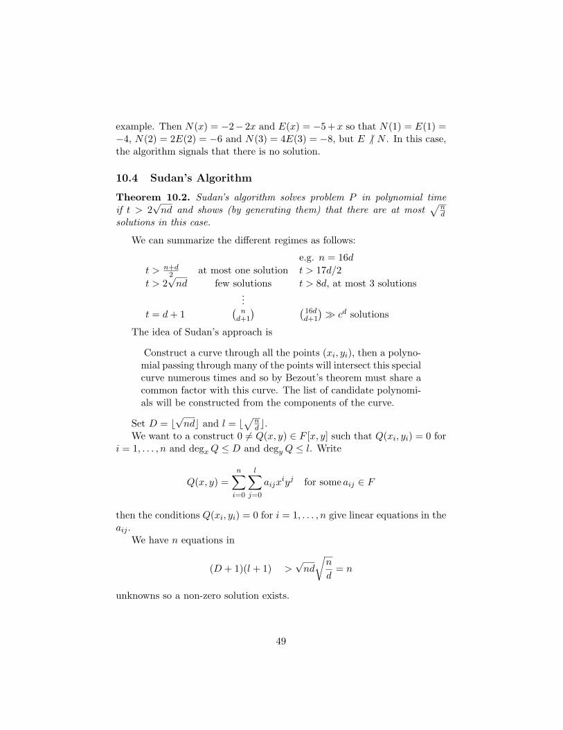
example. Then N(x) = −2− 2x and E(x) = −5+x so that N(1) = E(1) =−4, N(2) = 2E(2) = −6 and N(3) = 4E(3) = −8, but E 6 | N . In this case,the algorithm signals that there is no solution.

10.4 Sudan’s Algorithm

Theorem 10.2. Sudan’s algorithm solves problem P in polynomial timeif t > 2

√nd and shows (by generating them) that there are at most

√nd

solutions in this case.

We can summarize the different regimes as follows:

e.g. n = 16d

t > n+d2 at most one solution t > 17d/2

t > 2√

nd few solutions t > 8d, at most 3 solutions...

t = d + 1(

nd+1

) (16dd+1

)� cd solutions

The idea of Sudan’s approach is

Construct a curve through all the points (xi, yi), then a polyno-mial passing through many of the points will intersect this specialcurve numerous times and so by Bezout’s theorem must share acommon factor with this curve. The list of candidate polynomi-als will be constructed from the components of the curve.

Set D = b√

ndc and l = b√

nd c.

We want to a construct 0 6= Q(x, y) ∈ F [x, y] such that Q(xi, yi) = 0 fori = 1, . . . , n and degx Q ≤ D and degy Q ≤ l. Write

Q(x, y) =n∑

i=0

l∑j=0

aijxiyj for some aij ∈ F

then the conditions Q(xi, yi) = 0 for i = 1, . . . , n give linear equations in theaij .

We have n equations in

(D + 1)(l + 1) >√

nd

√n

d= n

unknowns so a non-zero solution exists.

49

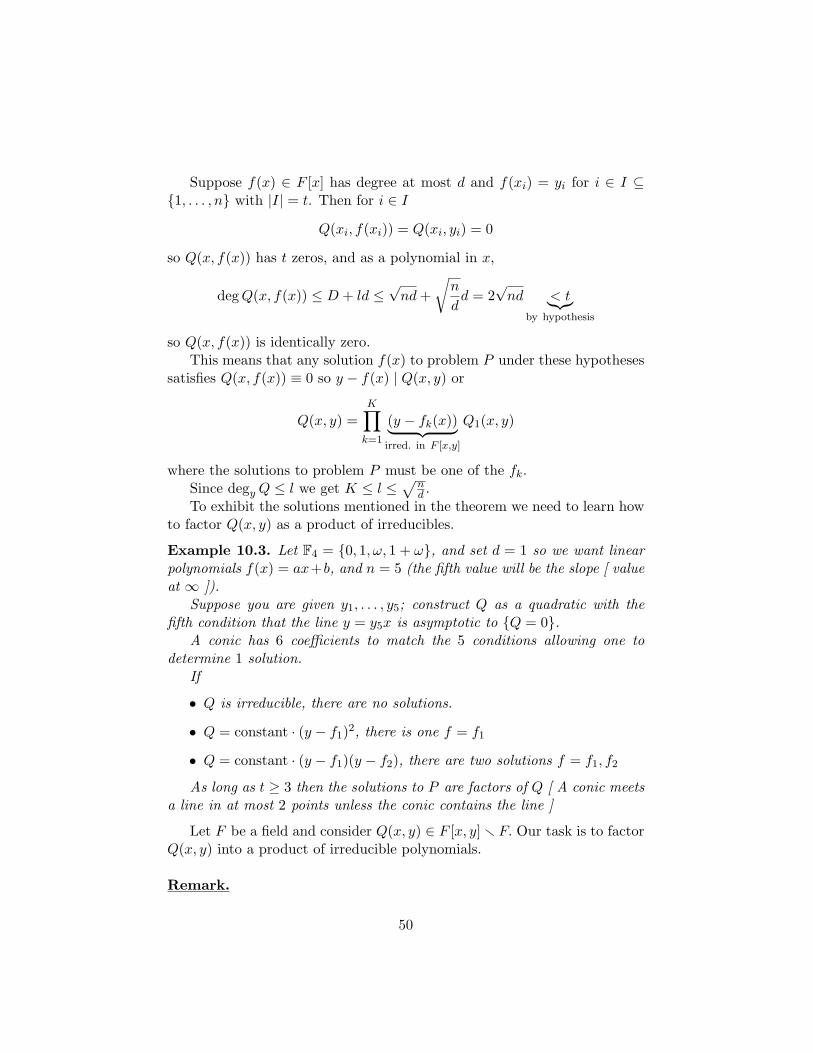
Suppose f(x) ∈ F [x] has degree at most d and f(xi) = yi for i ∈ I ⊆{1, . . . , n} with |I| = t. Then for i ∈ I

Q(xi, f(xi)) = Q(xi, yi) = 0

so Q(x, f(x)) has t zeros, and as a polynomial in x,

deg Q(x, f(x)) ≤ D + ld ≤√

nd +√

n

dd = 2

√nd < t︸︷︷︸

by hypothesis

so Q(x, f(x)) is identically zero.This means that any solution f(x) to problem P under these hypotheses

satisfies Q(x, f(x)) ≡ 0 so y − f(x) | Q(x, y) or

Q(x, y) =K∏

k=1

(y − fk(x))︸ ︷︷ ︸irred. in F [x,y]

Q1(x, y)

where the solutions to problem P must be one of the fk.Since degy Q ≤ l we get K ≤ l ≤

√nd .

To exhibit the solutions mentioned in the theorem we need to learn howto factor Q(x, y) as a product of irreducibles.

Example 10.3. Let F4 = {0, 1, ω, 1 + ω}, and set d = 1 so we want linearpolynomials f(x) = ax+b, and n = 5 (the fifth value will be the slope [ valueat ∞ ]).

Suppose you are given y1, . . . , y5; construct Q as a quadratic with thefifth condition that the line y = y5x is asymptotic to {Q = 0}.

A conic has 6 coefficients to match the 5 conditions allowing one todetermine 1 solution.

If

• Q is irreducible, there are no solutions.

• Q = constant · (y − f1)2, there is one f = f1

• Q = constant · (y − f1)(y − f2), there are two solutions f = f1, f2

As long as t ≥ 3 then the solutions to P are factors of Q [ A conic meetsa line in at most 2 points unless the conic contains the line ]

Let F be a field and consider Q(x, y) ∈ F [x, y] r F. Our task is to factorQ(x, y) into a product of irreducible polynomials.

Remark.

50

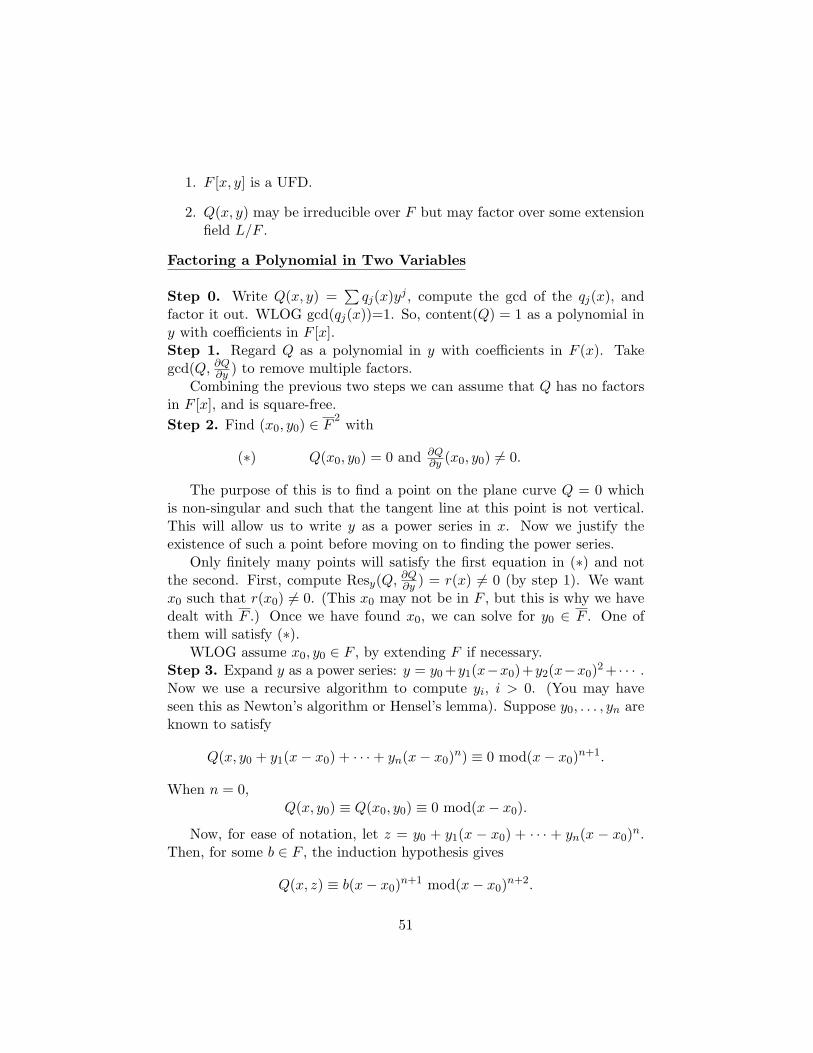
1. F [x, y] is a UFD.

2. Q(x, y) may be irreducible over F but may factor over some extensionfield L/F .

Factoring a Polynomial in Two Variables

Step 0. Write Q(x, y) =∑

qj(x)yj , compute the gcd of the qj(x), andfactor it out. WLOG gcd(qj(x))=1. So, content(Q) = 1 as a polynomial iny with coefficients in F [x].Step 1. Regard Q as a polynomial in y with coefficients in F (x). Takegcd(Q, ∂Q

∂y ) to remove multiple factors.Combining the previous two steps we can assume that Q has no factors

in F [x], and is square-free.Step 2. Find (x0, y0) ∈ F

2 with

(∗) Q(x0, y0) = 0 and ∂Q∂y (x0, y0) 6= 0.

The purpose of this is to find a point on the plane curve Q = 0 whichis non-singular and such that the tangent line at this point is not vertical.This will allow us to write y as a power series in x. Now we justify theexistence of such a point before moving on to finding the power series.

Only finitely many points will satisfy the first equation in (∗) and notthe second. First, compute Resy(Q, ∂Q

∂y ) = r(x) 6= 0 (by step 1). We wantx0 such that r(x0) 6= 0. (This x0 may not be in F , but this is why we havedealt with F .) Once we have found x0, we can solve for y0 ∈ F . One ofthem will satisfy (∗).

WLOG assume x0, y0 ∈ F , by extending F if necessary.Step 3. Expand y as a power series: y = y0 +y1(x−x0)+y2(x−x0)2 + · · · .Now we use a recursive algorithm to compute yi, i > 0. (You may haveseen this as Newton’s algorithm or Hensel’s lemma). Suppose y0, . . . , yn areknown to satisfy

Q(x, y0 + y1(x− x0) + · · ·+ yn(x− x0)n) ≡ 0 mod(x− x0)n+1.

When n = 0,Q(x, y0) ≡ Q(x0, y0) ≡ 0 mod(x− x0).

Now, for ease of notation, let z = y0 + y1(x − x0) + · · · + yn(x − x0)n.Then, for some b ∈ F , the induction hypothesis gives

Q(x, z) ≡ b(x− x0)n+1 mod(x− x0)n+2.

51

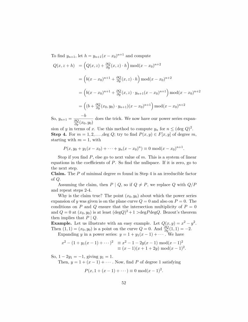
To find yn+1, let h = yn+1(x− x0)n+1 and compute

Q(x, z + h) =(Q(x, z) + ∂Q

∂y (x, z) · h)

mod(x− x0)n+2

=(b(x− x0)n+1 + ∂Q

∂y (x, z) · h)

mod(x− x0)n+2

=(b(x− x0)n+1 + ∂Q

∂y (x, z) · yn+1(x− x0)n+1)

mod(x− x0)n+2

=((b + ∂Q

∂y (x0, y0) · yn+1)(x− x0)n+1)

mod(x− x0)n+2

So, yn+1 =−b

∂Q∂y (x0, y0)

does the trick. We now have our power series expan-

sion of y in terms of x. Use this method to compute yn for n ≤ (deg Q)2.Step 4. For m = 1, 2, . . . ,deg Q; try to find P (x, y) ∈ F [x, y] of degree m,starting with m = 1, with

P (x, y0 + y1(x− x0) + · · ·+ yn(x− x0)n) ≡ 0 mod(x− x0)n+1.

Stop if you find P , else go to next value of m. This is a system of linearequations in the coefficients of P . So find the nullspace. If it is zero, go tothe next step.Claim. The P of minimal degree m found in Step 4 is an irreducible factorof Q.

Assuming the claim, then P | Q, so if Q 6= P , we replace Q with Q/Pand repeat steps 2-4.

Why is the claim true? The point (x0, y0) about which the power seriesexpansion of y was given is on the plane curve Q = 0 and also on P = 0. Theconditions on P and Q ensure that the intersection multiplicity of P = 0and Q = 0 at (x0, y0) is at least (degQ)2 +1 >degPdegQ. Bezout’s theoremthen implies that P | Q.Example. Let us illustrate with an easy example. Let Q(x, y) = x2 − y2.Then (1, 1) = (x0, y0) is a point on the curve Q = 0. And ∂Q

∂y (1, 1) = −2.Expanding y in a power series: y = 1 + y1(x− 1) + · · · . We have

x2 − (1 + y1(x− 1) + · · · )2 ≡ x2 − 1− 2y(x− 1) mod(x− 1)2

≡ (x− 1)(x + 1 + 2y) mod(x− 1)2.

So, 1− 2y1 = −1, giving y1 = 1.Then, y = 1 + (x− 1) + · · · . Now, find P of degree 1 satisfying

P (x, 1 + (x− 1) + · · · ) ≡ 0 mod(x− 1)2.

52

Say, P (x, y) = y − x, so P | Q.

A few weeks ago, we talked about how to factor in Z[x]. So, Q(Y ) ∈ Z[Y ].The analogy here is between Z and F[x]. Find a prime p and a y0 such that

Q(y0) = 0 mod pQ′(y0) 6= 0 mod p.

This is the same as finding (x0, y0). Now, use Hensel’s lemma: find y ∈ Z/pn

with Q(y) ≡ 0 mod pn, for n large in relation to the coefficients of Q. Step3 is to find the power series expansion of y:

y = y0 + y1p + y2p2 + · · ·+ ynpn

Now find P (Y ) ∈ Z[Y ] of small degree and with small coefficients such thatP (y) ≡ 0 mod pn. (This can no longer be done with linear algebra.) Thiscongruence defines a lattice in ZdegP+1. To find a short vector in a lattice,there is an algorithm called the LLL-algorithm which we won’t explain.Then a height calculation will replace Bezout to prove that P | Q.

11 List decoding and discrete log problem:

The decoding problem of Reed Solomon codes can be reformulated into theproblem of curve fitting or polynomial reconstruction. If we are given npoints, (x1, y1), (x2, y2)..., (xn, yn) in F2

q , we want to find all polynomialsf(x) of degree d that pass through at least t points. Recall that Sudan gavean algorithm for t ≥ 2

√nd. Cheng and Wan prove that if we decrease t much

further(made precise later), then decoding Reed Solomon codes becomes ashard as solving the discrete log problem.

11.1 Index Calculus versus Sudan’s algorithm

We use the index calculus technique for F∗q where , Fq = Fpn = Fp[x]/(f(x)).We consider p midsize, which means that log p and nα are of comparablesize.

We want to use the factor base

B = {g, x, x + 1, ....x + p− 1}

< g >= F∗p

53

The first question is how often h(x) of deg h ≤ n factors as

h(x) = gbp−1∏i=0

(x + i)ai

Total number of h’s is (pn − 1).The number of h’s which factor is (p− 1)

(n+p−1

p

)If p is big, n is small, this is approximately equal to pn

n! or cp when p and nare comparable.Probability of h factoring = 1

n! .But we want the polynomial to factor in the factor base in F∗q which is

weaker than factoring in Fp[x].Cheng’s Idea: Lets ask what it means to write h as a product of

elements in B in the quotient ring?

h(x) = gbp−1∏i=0

(x + i)ai + f(x)k(x) 1

But this is not useful to us because we don’t know k.However, if ai 6= 0, for some i = 0, 1, ..., p− 1,

h(−i) = f(−i)k(−i)

So,

k(−i) =h(−i)f(−i)

So, though we don’t know k, we know many of the values of k at elementsof Fp. This works only when many ai’s are non-zero.

Question: Reconstruct k(x) given that we know k(−i) for all i = 0, ..., p−1 with ai 6= 0.

d = deg k(x) =∑

ai − n

t = #{i = 0....p− 1|ai 6= 0}

Sudan’s algorithm produces a list of solutions k to polynomial recon-struction problem k(−i) = h(−i)/f(−i) for t values of i provided t ≥ 2

√pd

and the list has at most√

pd elements.

If,

k(−i) =h(−i)f(−i)

, i ∈ I ⊂ {0, 1..., p− 1}, |I| = t

54

We can deduce k(x)f(x) − h(x) vanishes at x = −i, i ∈ I. This only givesus:

k(x)f(x)− h(x) = gb∏i∈I

(x + i)u(x)

This is not quite enough. We want to get rid of u(x).

11.2 How to improve the index calculus algorithm

Fix some d. Given h(x) 6= 0 and deg h < n.Try to find all k(x) of degree ≤ d, such that

k(−i) =h(−i)f(−i)

for at least d2√

pde values of i and check whether k(x)f(x)−h(x) factors asa product of elements in the factor base.Note that if d is small, it is better to use Berlekamp’s algorithm than Sudan’s.

Problem: Count how many more factorizations we are going to achieveby this improvement.

2√

pd < t < p

Thusd <

p

4List decoding will not succeed if d > p

4 .

Theorem. If p > max(g2, (n− 1)2+ε) and g ≥ (4ε + 2)(n + 1) for some

ε > 0, then ∀h,∃k, ai, b, satisfying equation 1 with∑

ai ≤ g .

Question: Can this be improved?Gain: Count the possible ai with

∑ai ≤ (n + d) and with #{ai 6= 0} ≥

2√

pd. The good h’s are (gb)∏

(x + i)ai%f

11.3 Open questions

Consider: F∗pn , Fpn = Fp[x]/f(x). Let B be the set of monic irreduciblepolynomials with degree at most b. h(x) = gr

∏r(x)∈B r(x)αr + f(x)k(x)

k(z) = h(z)f(z) if r(z) = 0 and αr > 0

Sudan’s algorithm gives solution for the field in which we are working.Is there a version of Sudan’s algorithm taking into account the field wherethe values are? Can we use it for the discrete log problem?

55

11.4 Numerical example of Cheng’s idea:

Consider the field F125 = F53 = F5[x]/(x3 − x + 2). Instead of working withF∗125, we will work with G = F∗125/F∗5. Thus, |G| = 31 = 124/4

G =< x >. Factor Base B = x, x + 1, x + 2, x + 3, x + 4. Also, deg h(x) ≤2We ask the following questions: Does h(x) factor over B? How many h(x)factor over B as polynomials? The number of h(x) that factor over B aspolynomials are 1(constant) + 5(elements of B,linear) +5(squares)+ 10(2distinct factors)=21.So there are 10 irreducible polynomials of degree 2.

How many of these h can be expressed as

h(x) = c

4∏i=0

(x + i)ai + f(x)k(x)

with c, k ∈ F∗5 ? deg f = 3,deg h = 2,∑

ai = 3.Example 1: Consider h(x) = x2 + 3. Remember f(x) = x3 − x + 2.

The values of h(−i)/f(−i) for i = 1, 2, 3, 4, 0 are 2, 2, 4, 2, 4The degree of k is 0, and we try value k = 2 which works.

Example 2: h(x) = x2 + 2.The values of h(−i)/f(−i) for i = 1, 2, 3, 4, 0 are 4, 1, 2, 4, 1Try k = 4. We get h(x)− 4f(x) = (−4)(x + 1)2(x + 4).

Example 3: h(x) = x2 + 3x + 4.The values of h(−i)/f(−i) for i = 1, 2, 3, 4, 0 are 1, 2, 3, 4, 2Try k = 2 h(x)− 2f(x) = −2(x2)(x + 2). Here, another interesting observa-tion was that the values 1, 2, 3, 4 correspond to the values of the polynomial−x. So we also get: h(x) + xf(x) = (x + 1)(x + 2)(x + 3)(x + 4).

12 Complexity of Multiplication

Suppose V = {v1, ..., vn} is a basis of Fqn/Fq. So every element of Fqn is∑aivi ai ∈ Fq.

(∑

aivi)(∑

bivi) =∑

aibjvivj (13)

Now we need to know how to multiply the basis elements. Suppose:

vivj =∑

mijkvk, (14)

56

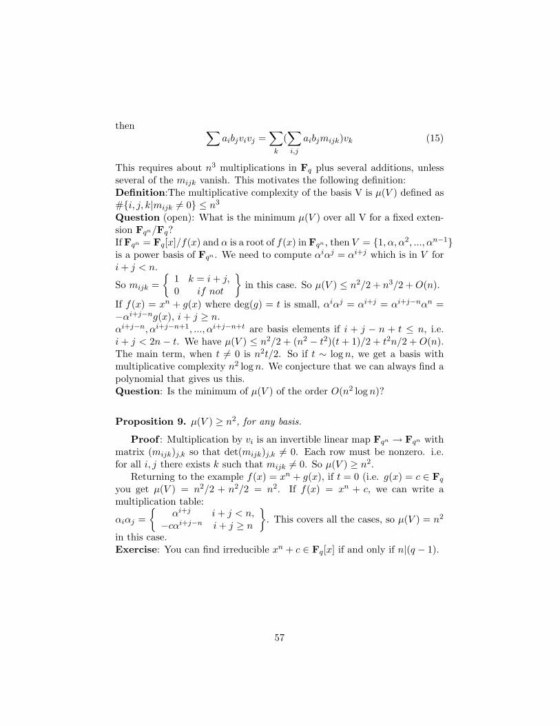
then ∑aibjvivj =

∑k

(∑i,j

aibjmijk)vk (15)

This requires about n3 multiplications in Fq plus several additions, unlessseveral of the mijk vanish. This motivates the following definition:Definition:The multiplicative complexity of the basis V is µ(V ) defined as#{i, j, k|mijk 6= 0} ≤ n3

Question (open): What is the minimum µ(V ) over all V for a fixed exten-sion Fqn/Fq?If Fqn = Fq[x]/f(x) and α is a root of f(x) in Fqn , then V = {1, α, α2, ..., αn−1}is a power basis of Fqn . We need to compute αiαj = αi+j which is in V fori + j < n.

So mijk ={

1 k = i + j,0 if not

}in this case. So µ(V ) ≤ n2/2 + n3/2 + O(n).

If f(x) = xn + g(x) where deg(g) = t is small, αiαj = αi+j = αi+j−nαn =−αi+j−ng(x), i + j ≥ n.αi+j−n, αi+j−n+1, ..., αi+j−n+t are basis elements if i + j − n + t ≤ n, i.e.i + j < 2n− t. We have µ(V ) ≤ n2/2 + (n2 − t2)(t + 1)/2 + t2n/2 + O(n).The main term, when t 6= 0 is n2t/2. So if t ∼ log n, we get a basis withmultiplicative complexity n2 log n. We conjecture that we can always find apolynomial that gives us this.Question: Is the minimum of µ(V ) of the order O(n2 log n)?

Proposition 9. µ(V ) ≥ n2, for any basis.

Proof : Multiplication by vi is an invertible linear map Fqn → Fqn withmatrix (mijk)j,k so that det(mijk)j,k 6= 0. Each row must be nonzero. i.e.for all i, j there exists k such that mijk 6= 0. So µ(V ) ≥ n2.

Returning to the example f(x) = xn + g(x), if t = 0 (i.e. g(x) = c ∈ Fq

you get µ(V ) = n2/2 + n2/2 = n2. If f(x) = xn + c, we can write amultiplication table:

αiαj ={

αi+j i + j < n,−cαi+j−n i + j ≥ n

}. This covers all the cases, so µ(V ) = n2

in this case.Exercise: You can find irreducible xn + c ∈ Fq[x] if and only if n|(q − 1).

57

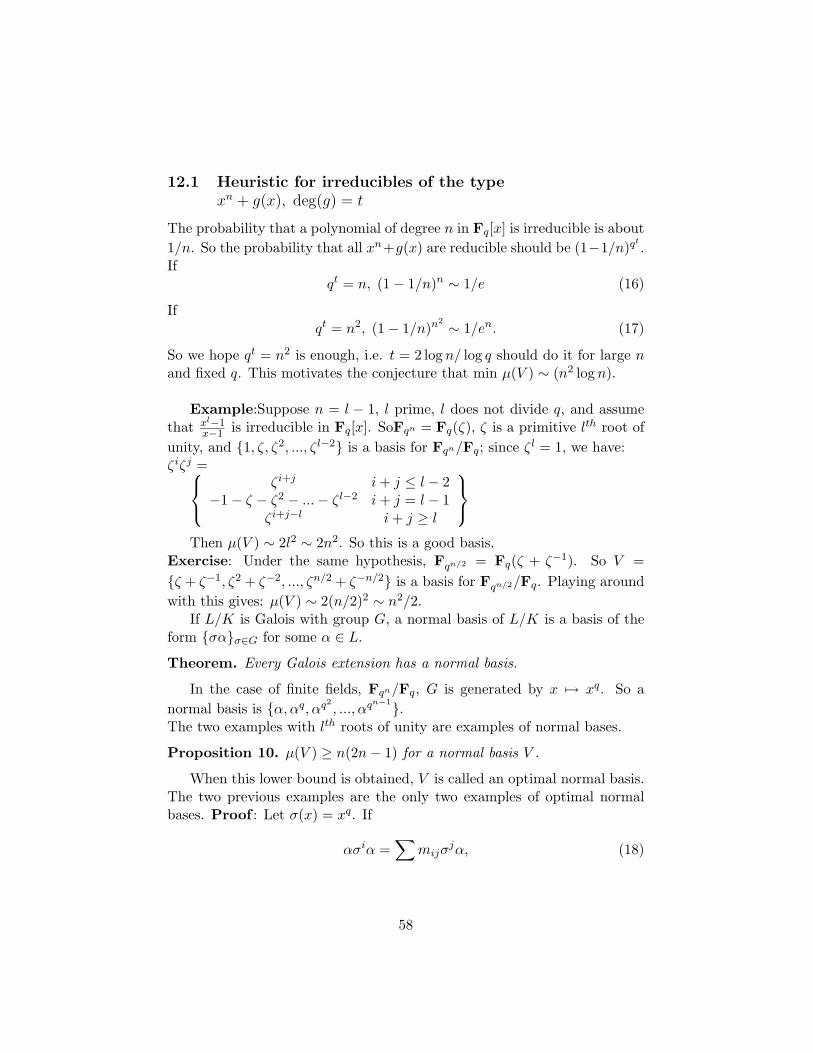
12.1 Heuristic for irreducibles of the typexn + g(x), deg(g) = t

The probability that a polynomial of degree n in Fq[x] is irreducible is about1/n. So the probability that all xn+g(x) are reducible should be (1−1/n)qt

.If

qt = n, (1− 1/n)n ∼ 1/e (16)

Ifqt = n2, (1− 1/n)n2 ∼ 1/en. (17)

So we hope qt = n2 is enough, i.e. t = 2 log n/ log q should do it for large nand fixed q. This motivates the conjecture that min µ(V ) ∼ (n2 log n).

Example:Suppose n = l − 1, l prime, l does not divide q, and assumethat xl−1

x−1 is irreducible in Fq[x]. SoFqn = Fq(ζ), ζ is a primitive lth root ofunity, and {1, ζ, ζ2, ..., ζ l−2} is a basis for Fqn/Fq; since ζ l = 1, we have:ζiζj =

ζi+j i + j ≤ l − 2−1− ζ − ζ2 − ...− ζ l−2 i + j = l − 1

ζi+j−l i + j ≥ l

Then µ(V ) ∼ 2l2 ∼ 2n2. So this is a good basis.

Exercise: Under the same hypothesis, Fqn/2 = Fq(ζ + ζ−1). So V ={ζ + ζ−1, ζ2 + ζ−2, ..., ζn/2 + ζ−n/2} is a basis for Fqn/2/Fq. Playing aroundwith this gives: µ(V ) ∼ 2(n/2)2 ∼ n2/2.

If L/K is Galois with group G, a normal basis of L/K is a basis of theform {σα}σ∈G for some α ∈ L.

Theorem. Every Galois extension has a normal basis.

In the case of finite fields, Fqn/Fq, G is generated by x 7→ xq. So anormal basis is {α, αq, αq2

, ..., αqn−1}.The two examples with lth roots of unity are examples of normal bases.

Proposition 10. µ(V ) ≥ n(2n− 1) for a normal basis V .

When this lower bound is obtained, V is called an optimal normal basis.The two previous examples are the only two examples of optimal normalbases. Proof : Let σ(x) = xq. If

ασiα =∑

mijσjα, (18)

58

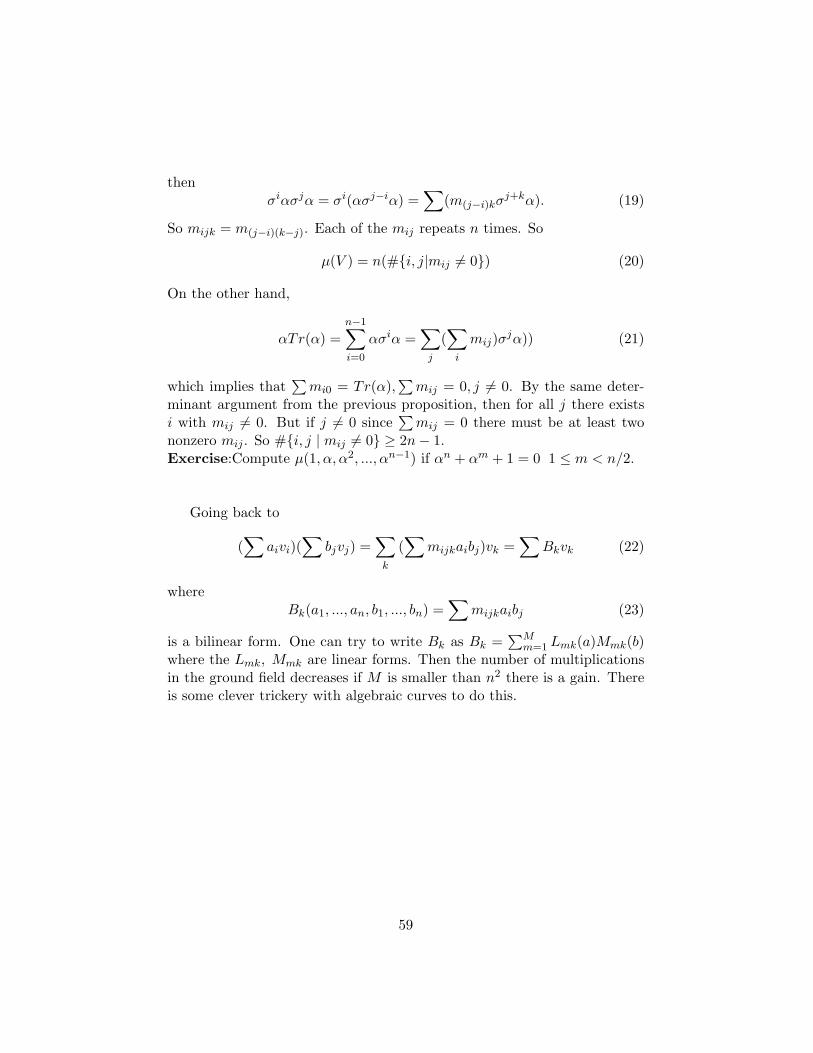
thenσiασjα = σi(ασj−iα) =

∑(m(j−i)kσ

j+kα). (19)

So mijk = m(j−i)(k−j). Each of the mij repeats n times. So

µ(V ) = n(#{i, j|mij 6= 0}) (20)

On the other hand,

αTr(α) =n−1∑i=0

ασiα =∑

j

(∑

i

mij)σjα)) (21)

which implies that∑

mi0 = Tr(α),∑

mij = 0, j 6= 0. By the same deter-minant argument from the previous proposition, then for all j there existsi with mij 6= 0. But if j 6= 0 since

∑mij = 0 there must be at least two

nonzero mij . So #{i, j | mij 6= 0} ≥ 2n− 1.Exercise:Compute µ(1, α, α2, ..., αn−1) if αn + αm + 1 = 0 1 ≤ m < n/2.

Going back to

(∑

aivi)(∑

bjvj) =∑

k

(∑

mijkaibj)vk =∑

Bkvk (22)

whereBk(a1, ..., an, b1, ..., bn) =

∑mijkaibj (23)

is a bilinear form. One can try to write Bk as Bk =∑M

m=1 Lmk(a)Mmk(b)where the Lmk, Mmk are linear forms. Then the number of multiplicationsin the ground field decreases if M is smaller than n2 there is a gain. Thereis some clever trickery with algebraic curves to do this.

59