Embed Size (px)
Citation preview
MATH 361: Financial Mathematics for Actuaries I
Albert Cohen
Actuarial Sciences ProgramDepartment of Mathematics
Department of Statistics and ProbabilityC336 Wells Hall
Michigan State UniversityEast Lansing MI
[email protected]@stt.msu.edu
Albert Cohen (MSU) Financial Mathematics for Actuaries I MSU Fall 2017 1 / 164

Course Information
Syllabus to be posted on class page in first week of classes
Homework assignments will posted there as well
Page can be found at https://math.msu.edu/classpages/
Albert Cohen (MSU) Financial Mathematics for Actuaries I MSU Fall 2017 2 / 164
Course Information
Many examples within these slides are used with kind permission ofProf. Dmitry Kramkov, Dept. of Mathematics, Carnegie MellonUniversity.
Book for course: Marcel Finan’s A Discussion of Financial Economicsin Actuarial Models: A Preparation for the Actuarial Exam MFE/3F.Some proofs from there will be referenced as well. Please find thesenotes here
Some examples here will be similar to those practice questionspublicly released by the SOA. Please note the SOA owns thecopyright to these questions.
Albert Cohen (MSU) Financial Mathematics for Actuaries I MSU Fall 2017 3 / 164

What are financial securities?
Traded Securities - price given by market.
For example:
StocksCommodities
Non-Traded Securities - price remains to be computed.
Is this always true?
We will focus on pricing non-traded securities.
Albert Cohen (MSU) Financial Mathematics for Actuaries I MSU Fall 2017 4 / 164

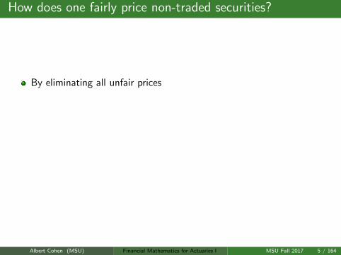
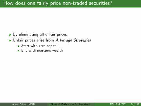
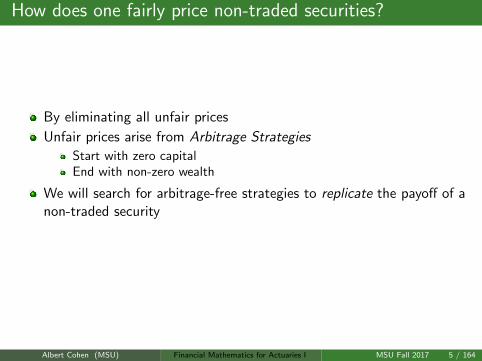
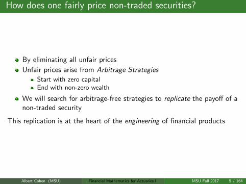
How does one fairly price non-traded securities?
By eliminating all unfair prices
Unfair prices arise from Arbitrage Strategies
Start with zero capitalEnd with non-zero wealth
We will search for arbitrage-free strategies to replicate the payoff of anon-traded security
This replication is at the heart of the engineering of financial products
Albert Cohen (MSU) Financial Mathematics for Actuaries I MSU Fall 2017 5 / 164
More Questions
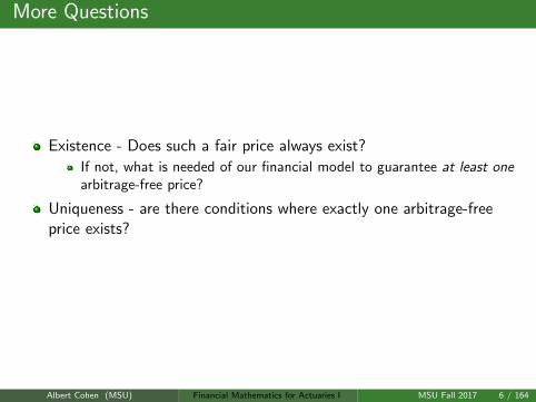
Existence - Does such a fair price always exist?
If not, what is needed of our financial model to guarantee at least onearbitrage-free price?
Uniqueness - are there conditions where exactly one arbitrage-freeprice exists?
Albert Cohen (MSU) Financial Mathematics for Actuaries I MSU Fall 2017 6 / 164

And What About...
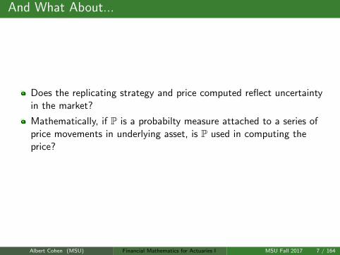
Does the replicating strategy and price computed reflect uncertaintyin the market?
Mathematically, if P is a probabilty measure attached to a series ofprice movements in underlying asset, is P used in computing theprice?
Albert Cohen (MSU) Financial Mathematics for Actuaries I MSU Fall 2017 7 / 164
And What About...
Does the replicating strategy and price computed reflect uncertaintyin the market?
Mathematically, if P is a probabilty measure attached to a series ofprice movements in underlying asset, is P used in computing theprice?
Albert Cohen (MSU) Financial Mathematics for Actuaries I MSU Fall 2017 7 / 164

Notation
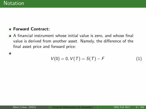
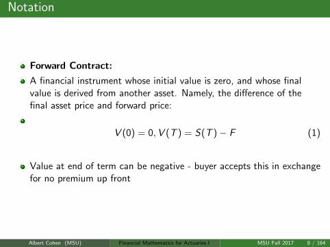
Forward Contract:
A financial instrument whose initial value is zero, and whose finalvalue is derived from another asset. Namely, the difference of thefinal asset price and forward price:
V (0) = 0,V (T ) = S(T )− F (1)
Value at end of term can be negative - buyer accepts this in exchangefor no premium up front
Albert Cohen (MSU) Financial Mathematics for Actuaries I MSU Fall 2017 8 / 164
Notation
Forward Contract:
A financial instrument whose initial value is zero, and whose finalvalue is derived from another asset. Namely, the difference of thefinal asset price and forward price:
V (0) = 0,V (T ) = S(T )− F (1)
Value at end of term can be negative - buyer accepts this in exchangefor no premium up front
Albert Cohen (MSU) Financial Mathematics for Actuaries I MSU Fall 2017 8 / 164

Notation
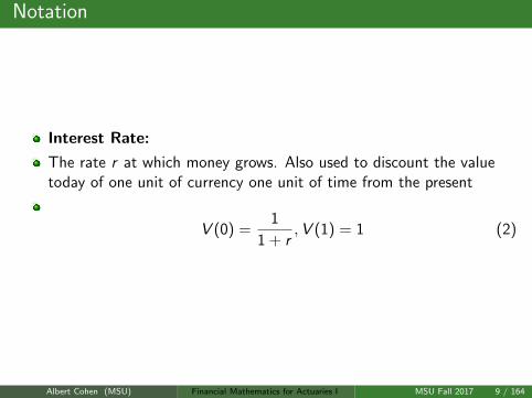
Interest Rate:
The rate r at which money grows. Also used to discount the valuetoday of one unit of currency one unit of time from the present
V (0) =1
1 + r,V (1) = 1 (2)
Albert Cohen (MSU) Financial Mathematics for Actuaries I MSU Fall 2017 9 / 164
Notation
Interest Rate:
The rate r at which money grows. Also used to discount the valuetoday of one unit of currency one unit of time from the present
V (0) =1
1 + r,V (1) = 1 (2)
Albert Cohen (MSU) Financial Mathematics for Actuaries I MSU Fall 2017 9 / 164
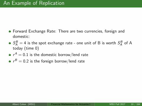
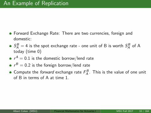
An Example of Replication
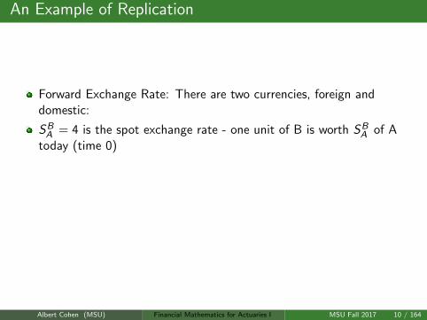
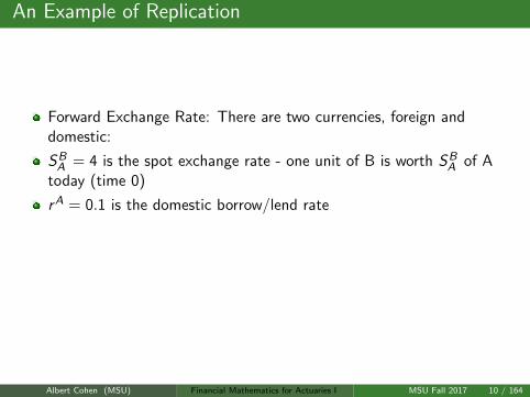
Forward Exchange Rate: There are two currencies, foreign anddomestic:
SBA = 4 is the spot exchange rate - one unit of B is worth SB
A of Atoday (time 0)
rA = 0.1 is the domestic borrow/lend rate
rB = 0.2 is the foreign borrow/lend rate
Compute the forward exchange rate FBA . This is the value of one unit
of B in terms of A at time 1.
Albert Cohen (MSU) Financial Mathematics for Actuaries I MSU Fall 2017 10 / 164
An Example of Replication
Forward Exchange Rate: There are two currencies, foreign anddomestic:
SBA = 4 is the spot exchange rate - one unit of B is worth SB
A of Atoday (time 0)
rA = 0.1 is the domestic borrow/lend rate
rB = 0.2 is the foreign borrow/lend rate
Compute the forward exchange rate FBA . This is the value of one unit
of B in terms of A at time 1.
Albert Cohen (MSU) Financial Mathematics for Actuaries I MSU Fall 2017 10 / 164
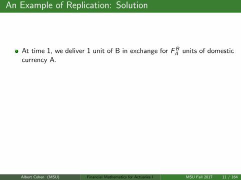
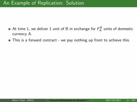
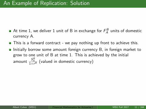
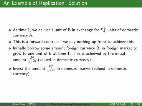
An Example of Replication: Solution
At time 1, we deliver 1 unit of B in exchange for FBA units of domestic
currency A.
This is a forward contract - we pay nothing up front to achieve this.
Initially borrow some amount foreign currency B, in foreign market togrow to one unit of B at time 1. This is achieved by the initial
amountSBA
1+rB(valued in domestic currency)
Invest the amountFBA
1+rAin domestic market (valued in domestic
currency)
Albert Cohen (MSU) Financial Mathematics for Actuaries I MSU Fall 2017 11 / 164

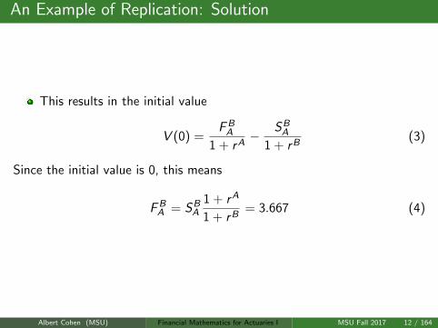
An Example of Replication: Solution
This results in the initial value
V (0) =FBA
1 + rA−
SBA
1 + rB(3)
Since the initial value is 0, this means
FBA = SB
A
1 + rA
1 + rB= 3.667 (4)
Albert Cohen (MSU) Financial Mathematics for Actuaries I MSU Fall 2017 12 / 164
An Example of Replication: Solution
This results in the initial value
V (0) =FBA
1 + rA−
SBA
1 + rB(3)
Since the initial value is 0, this means
FBA = SB
A
1 + rA
1 + rB= 3.667 (4)
Albert Cohen (MSU) Financial Mathematics for Actuaries I MSU Fall 2017 12 / 164

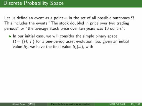
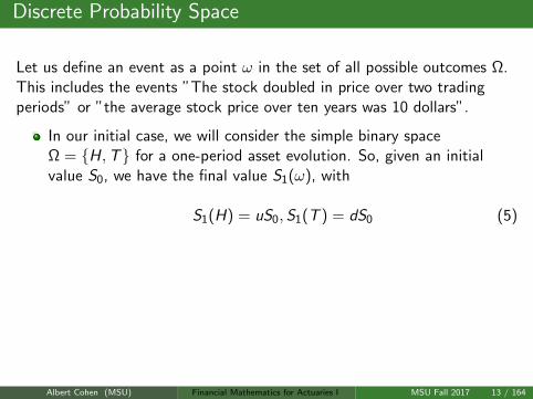
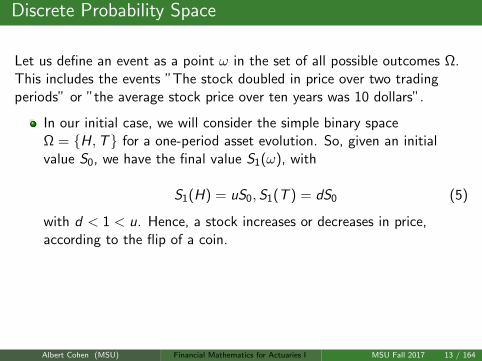
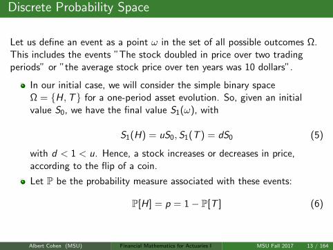
Discrete Probability Space
Let us define an event as a point ω in the set of all possible outcomes Ω.This includes the events ”The stock doubled in price over two tradingperiods” or ”the average stock price over ten years was 10 dollars”.
In our initial case, we will consider the simple binary spaceΩ = H,T for a one-period asset evolution. So, given an initialvalue S0, we have the final value S1(ω), with
S1(H) = uS0,S1(T ) = dS0 (5)
with d < 1 < u. Hence, a stock increases or decreases in price,according to the flip of a coin.
Let P be the probability measure associated with these events:
P[H] = p = 1− P[T ] (6)
Albert Cohen (MSU) Financial Mathematics for Actuaries I MSU Fall 2017 13 / 164
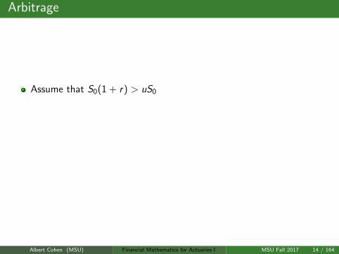
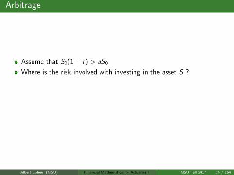
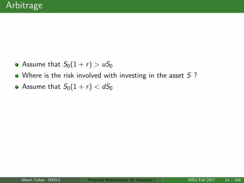
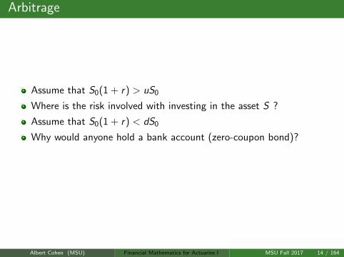
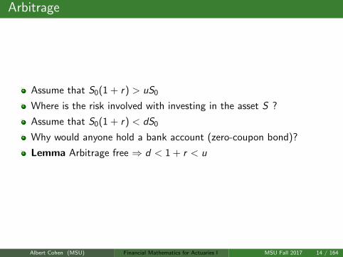
Arbitrage
Assume that S0(1 + r) > uS0
Where is the risk involved with investing in the asset S ?
Assume that S0(1 + r) < dS0
Why would anyone hold a bank account (zero-coupon bond)?
Lemma Arbitrage free ⇒ d < 1 + r < u
Albert Cohen (MSU) Financial Mathematics for Actuaries I MSU Fall 2017 14 / 164
Arbitrage
Assume that S0(1 + r) > uS0
Where is the risk involved with investing in the asset S ?
Assume that S0(1 + r) < dS0
Why would anyone hold a bank account (zero-coupon bond)?
Lemma Arbitrage free ⇒ d < 1 + r < u
Albert Cohen (MSU) Financial Mathematics for Actuaries I MSU Fall 2017 14 / 164
Arbitrage
Assume that S0(1 + r) > uS0
Where is the risk involved with investing in the asset S ?
Assume that S0(1 + r) < dS0
Why would anyone hold a bank account (zero-coupon bond)?
Lemma Arbitrage free ⇒ d < 1 + r < u
Albert Cohen (MSU) Financial Mathematics for Actuaries I MSU Fall 2017 14 / 164
Arbitrage
Assume that S0(1 + r) > uS0
Where is the risk involved with investing in the asset S ?
Assume that S0(1 + r) < dS0
Why would anyone hold a bank account (zero-coupon bond)?
Lemma Arbitrage free ⇒ d < 1 + r < u
Albert Cohen (MSU) Financial Mathematics for Actuaries I MSU Fall 2017 14 / 164
Arbitrage
Assume that S0(1 + r) > uS0
Where is the risk involved with investing in the asset S ?
Assume that S0(1 + r) < dS0
Why would anyone hold a bank account (zero-coupon bond)?
Lemma Arbitrage free ⇒ d < 1 + r < u
Albert Cohen (MSU) Financial Mathematics for Actuaries I MSU Fall 2017 14 / 164
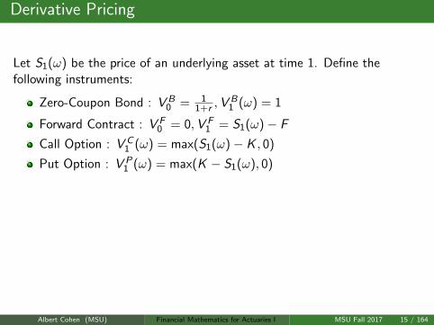
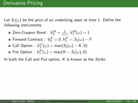
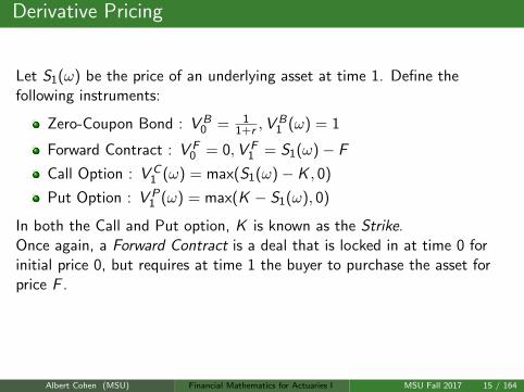
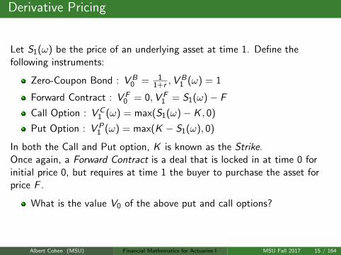
Derivative Pricing
Let S1(ω) be the price of an underlying asset at time 1. Define thefollowing instruments:
Zero-Coupon Bond : V B0 = 1
1+r ,VB1 (ω) = 1
Forward Contract : V F0 = 0,V F
1 = S1(ω)− F
Call Option : V C1 (ω) = max(S1(ω)− K , 0)
Put Option : V P1 (ω) = max(K − S1(ω), 0)
In both the Call and Put option, K is known as the Strike.Once again, a Forward Contract is a deal that is locked in at time 0 forinitial price 0, but requires at time 1 the buyer to purchase the asset forprice F .
What is the value V0 of the above put and call options?
Albert Cohen (MSU) Financial Mathematics for Actuaries I MSU Fall 2017 15 / 164
Derivative Pricing
Let S1(ω) be the price of an underlying asset at time 1. Define thefollowing instruments:
Zero-Coupon Bond : V B0 = 1
1+r ,VB1 (ω) = 1
Forward Contract : V F0 = 0,V F
1 = S1(ω)− F
Call Option : V C1 (ω) = max(S1(ω)− K , 0)
Put Option : V P1 (ω) = max(K − S1(ω), 0)
In both the Call and Put option, K is known as the Strike.
Once again, a Forward Contract is a deal that is locked in at time 0 forinitial price 0, but requires at time 1 the buyer to purchase the asset forprice F .
What is the value V0 of the above put and call options?
Albert Cohen (MSU) Financial Mathematics for Actuaries I MSU Fall 2017 15 / 164
Derivative Pricing
Let S1(ω) be the price of an underlying asset at time 1. Define thefollowing instruments:
Zero-Coupon Bond : V B0 = 1
1+r ,VB1 (ω) = 1
Forward Contract : V F0 = 0,V F
1 = S1(ω)− F
Call Option : V C1 (ω) = max(S1(ω)− K , 0)
Put Option : V P1 (ω) = max(K − S1(ω), 0)
In both the Call and Put option, K is known as the Strike.Once again, a Forward Contract is a deal that is locked in at time 0 forinitial price 0, but requires at time 1 the buyer to purchase the asset forprice F .
What is the value V0 of the above put and call options?
Albert Cohen (MSU) Financial Mathematics for Actuaries I MSU Fall 2017 15 / 164
Derivative Pricing
Let S1(ω) be the price of an underlying asset at time 1. Define thefollowing instruments:
Zero-Coupon Bond : V B0 = 1
1+r ,VB1 (ω) = 1
Forward Contract : V F0 = 0,V F
1 = S1(ω)− F
Call Option : V C1 (ω) = max(S1(ω)− K , 0)
Put Option : V P1 (ω) = max(K − S1(ω), 0)
In both the Call and Put option, K is known as the Strike.Once again, a Forward Contract is a deal that is locked in at time 0 forinitial price 0, but requires at time 1 the buyer to purchase the asset forprice F .
What is the value V0 of the above put and call options?
Albert Cohen (MSU) Financial Mathematics for Actuaries I MSU Fall 2017 15 / 164

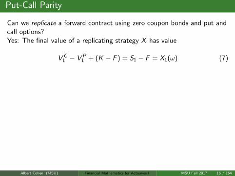
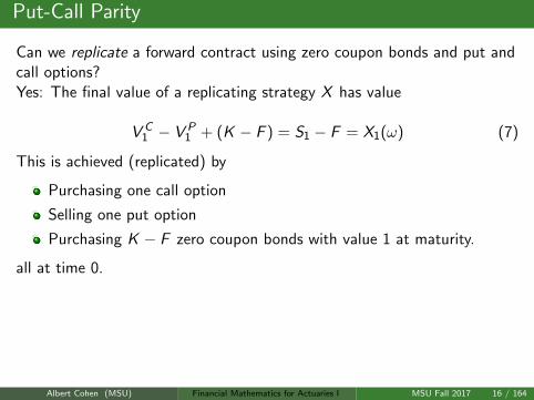
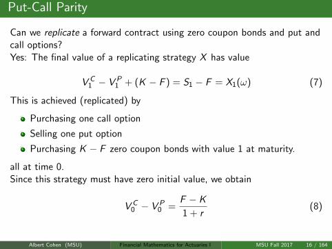
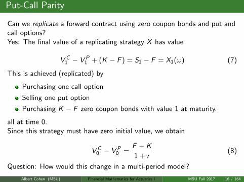
Put-Call Parity
Can we replicate a forward contract using zero coupon bonds and put andcall options?
Yes: The final value of a replicating strategy X has value
V C1 − V P
1 + (K − F ) = S1 − F = X1(ω) (7)
This is achieved (replicated) by
Purchasing one call option
Selling one put option
Purchasing K − F zero coupon bonds with value 1 at maturity.
all at time 0.Since this strategy must have zero initial value, we obtain
V C0 − V P
0 =F − K
1 + r(8)
Question: How would this change in a multi-period model?
Albert Cohen (MSU) Financial Mathematics for Actuaries I MSU Fall 2017 16 / 164
Put-Call Parity
Can we replicate a forward contract using zero coupon bonds and put andcall options?Yes: The final value of a replicating strategy X has value
V C1 − V P
1 + (K − F ) = S1 − F = X1(ω) (7)
This is achieved (replicated) by
Purchasing one call option
Selling one put option
Purchasing K − F zero coupon bonds with value 1 at maturity.
all at time 0.
Since this strategy must have zero initial value, we obtain
V C0 − V P
0 =F − K
1 + r(8)
Question: How would this change in a multi-period model?
Albert Cohen (MSU) Financial Mathematics for Actuaries I MSU Fall 2017 16 / 164
Put-Call Parity
Can we replicate a forward contract using zero coupon bonds and put andcall options?Yes: The final value of a replicating strategy X has value
V C1 − V P
1 + (K − F ) = S1 − F = X1(ω) (7)
This is achieved (replicated) by
Purchasing one call option
Selling one put option
Purchasing K − F zero coupon bonds with value 1 at maturity.
all at time 0.Since this strategy must have zero initial value, we obtain
V C0 − V P
0 =F − K
1 + r(8)
Question: How would this change in a multi-period model?
Albert Cohen (MSU) Financial Mathematics for Actuaries I MSU Fall 2017 16 / 164
Put-Call Parity
Can we replicate a forward contract using zero coupon bonds and put andcall options?Yes: The final value of a replicating strategy X has value
V C1 − V P
1 + (K − F ) = S1 − F = X1(ω) (7)
This is achieved (replicated) by
Purchasing one call option
Selling one put option
Purchasing K − F zero coupon bonds with value 1 at maturity.
all at time 0.Since this strategy must have zero initial value, we obtain
V C0 − V P
0 =F − K
1 + r(8)
Question: How would this change in a multi-period model?
Albert Cohen (MSU) Financial Mathematics for Actuaries I MSU Fall 2017 16 / 164
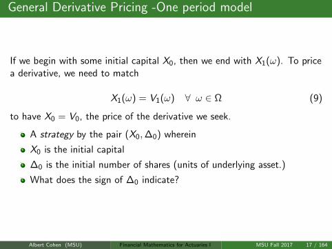
General Derivative Pricing -One period model
If we begin with some initial capital X0, then we end with X1(ω). To pricea derivative, we need to match
X1(ω) = V1(ω) ∀ ω ∈ Ω (9)
to have X0 = V0, the price of the derivative we seek.
A strategy by the pair (X0,∆0) wherein
X0 is the initial capital
∆0 is the initial number of shares (units of underlying asset.)
What does the sign of ∆0 indicate?
Albert Cohen (MSU) Financial Mathematics for Actuaries I MSU Fall 2017 17 / 164

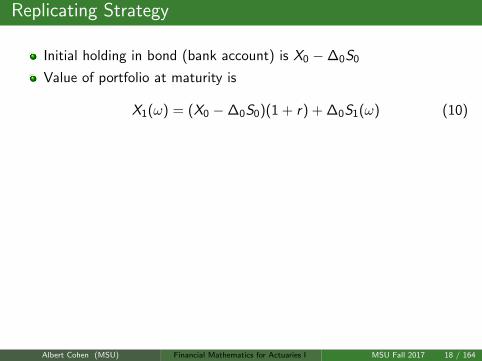
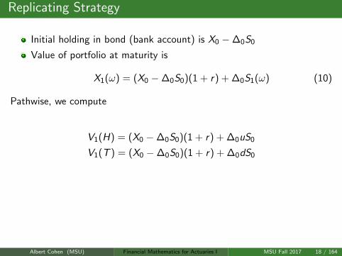
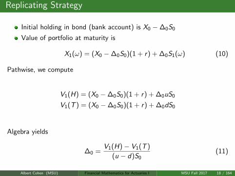
Replicating Strategy
Initial holding in bond (bank account) is X0 −∆0S0
Value of portfolio at maturity is
X1(ω) = (X0 −∆0S0)(1 + r) + ∆0S1(ω) (10)
Pathwise, we compute
V1(H) = (X0 −∆0S0)(1 + r) + ∆0uS0
V1(T ) = (X0 −∆0S0)(1 + r) + ∆0dS0
Algebra yields
∆0 =V1(H)− V1(T )
(u − d)S0(11)
Albert Cohen (MSU) Financial Mathematics for Actuaries I MSU Fall 2017 18 / 164
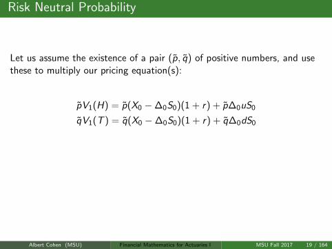
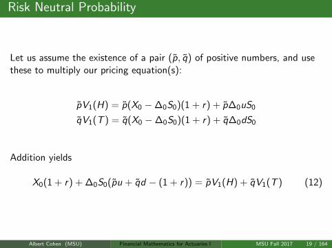
Risk Neutral Probability
Let us assume the existence of a pair (p, q) of positive numbers, and usethese to multiply our pricing equation(s):
pV1(H) = p(X0 −∆0S0)(1 + r) + p∆0uS0
qV1(T ) = q(X0 −∆0S0)(1 + r) + q∆0dS0
Addition yields
X0(1 + r) + ∆0S0(pu + qd − (1 + r)) = pV1(H) + qV1(T ) (12)
Albert Cohen (MSU) Financial Mathematics for Actuaries I MSU Fall 2017 19 / 164
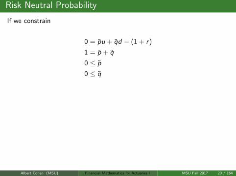
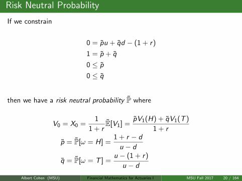
Risk Neutral Probability
If we constrain
0 = pu + qd − (1 + r)
1 = p + q
0 ≤ p
0 ≤ q
then we have a risk neutral probability P where
V0 = X0 =1
1 + rE[V1] =
pV1(H) + qV1(T )
1 + r
p = P[ω = H] =1 + r − d
u − d
q = P[ω = T ] =u − (1 + r)
u − d
Albert Cohen (MSU) Financial Mathematics for Actuaries I MSU Fall 2017 20 / 164
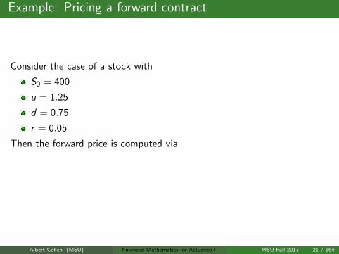
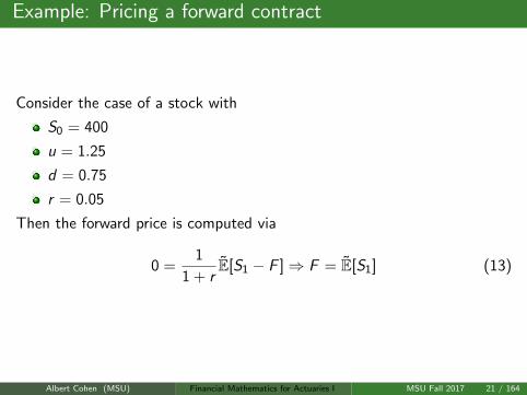
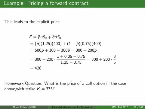
Example: Pricing a forward contract
Consider the case of a stock with
S0 = 400
u = 1.25
d = 0.75
r = 0.05
Then the forward price is computed via
0 =1
1 + rE[S1 − F ]⇒ F = E[S1] (13)
Albert Cohen (MSU) Financial Mathematics for Actuaries I MSU Fall 2017 21 / 164
Example: Pricing a forward contract
Consider the case of a stock with
S0 = 400
u = 1.25
d = 0.75
r = 0.05
Then the forward price is computed via
0 =1
1 + rE[S1 − F ]⇒ F = E[S1] (13)
Albert Cohen (MSU) Financial Mathematics for Actuaries I MSU Fall 2017 21 / 164
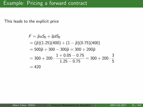
Example: Pricing a forward contract
This leads to the explicit price
F = puS0 + qdS0
= (p)(1.25)(400) + (1− p)(0.75)(400)
= 500p + 300− 300p = 300 + 200p
= 300 + 200 · 1 + 0.05− 0.75
1.25− 0.75= 300 + 200 · 3
5
= 420
Homework Question: What is the price of a call option in the caseabove,with strike K = 375?
Albert Cohen (MSU) Financial Mathematics for Actuaries I MSU Fall 2017 22 / 164
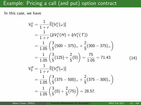
Example: Pricing a call (and put) option contract
In this case, we have
V c0 =
1
1 + rE[V c
1 (ω)]
=1
1 + r(pV c
1 (H) + qV c1 (T ))
=1
1.05
(3
5(500− 375)+ +
2
5(300− 375)+
)=
1
1.05
(3
5(125) +
2
5(0)
)=
75
1.05= 71.43
V p0 =
1
1 + rE[V p
1 (ω)]
=1
1.05
(3
5(375− 500)+ +
2
5(375− 300)+
)=
1
1.05
(3
5(0) +
2
5(75)
)= 28.57.
(14)
Albert Cohen (MSU) Financial Mathematics for Actuaries I MSU Fall 2017 23 / 164
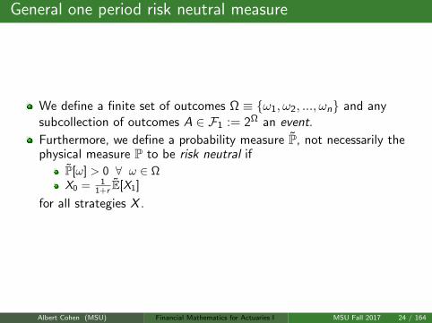
General one period risk neutral measure
We define a finite set of outcomes Ω ≡ ω1, ω2, ..., ωn and anysubcollection of outcomes A ∈ F1 := 2Ω an event.
Furthermore, we define a probability measure P, not necessarily thephysical measure P to be risk neutral if
P[ω] > 0 ∀ ω ∈ ΩX0 = 1
1+r E[X1]
for all strategies X .
Albert Cohen (MSU) Financial Mathematics for Actuaries I MSU Fall 2017 24 / 164
General one period risk neutral measure
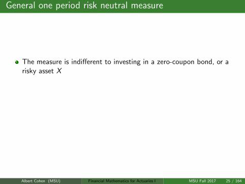
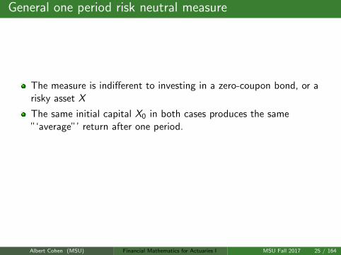
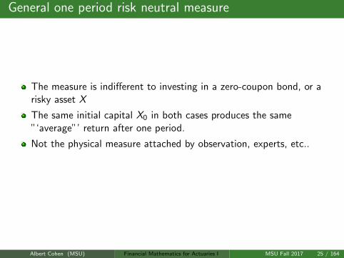
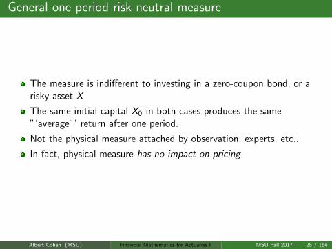
The measure is indifferent to investing in a zero-coupon bond, or arisky asset X
The same initial capital X0 in both cases produces the same”‘average”’ return after one period.
Not the physical measure attached by observation, experts, etc..
In fact, physical measure has no impact on pricing
Albert Cohen (MSU) Financial Mathematics for Actuaries I MSU Fall 2017 25 / 164
General one period risk neutral measure
The measure is indifferent to investing in a zero-coupon bond, or arisky asset X
The same initial capital X0 in both cases produces the same”‘average”’ return after one period.
Not the physical measure attached by observation, experts, etc..
In fact, physical measure has no impact on pricing
Albert Cohen (MSU) Financial Mathematics for Actuaries I MSU Fall 2017 25 / 164
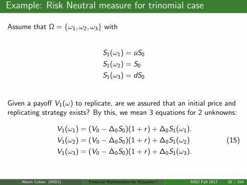
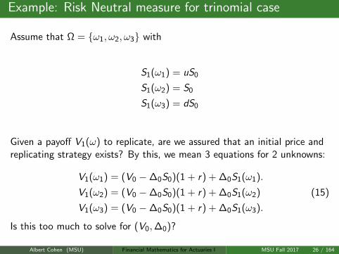
Example: Risk Neutral measure for trinomial case
Assume that Ω = ω1, ω2, ω3 with
S1(ω1) = uS0
S1(ω2) = S0
S1(ω3) = dS0
Given a payoff V1(ω) to replicate, are we assured that an initial price andreplicating strategy exists? By this, we mean 3 equations for 2 unknowns:
V1(ω1) = (V0 −∆0S0)(1 + r) + ∆0S1(ω1).
V1(ω2) = (V0 −∆0S0)(1 + r) + ∆0S1(ω2)
V1(ω3) = (V0 −∆0S0)(1 + r) + ∆0S1(ω3).
(15)
Is this too much to solve for (V0,∆0)?
Albert Cohen (MSU) Financial Mathematics for Actuaries I MSU Fall 2017 26 / 164
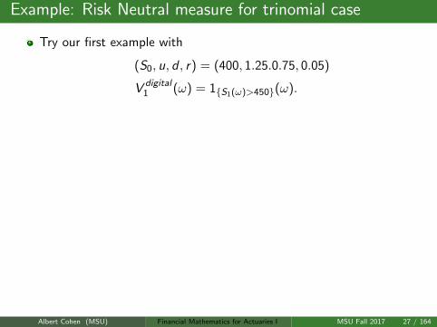
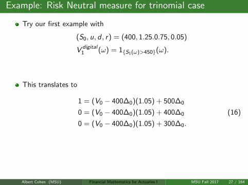
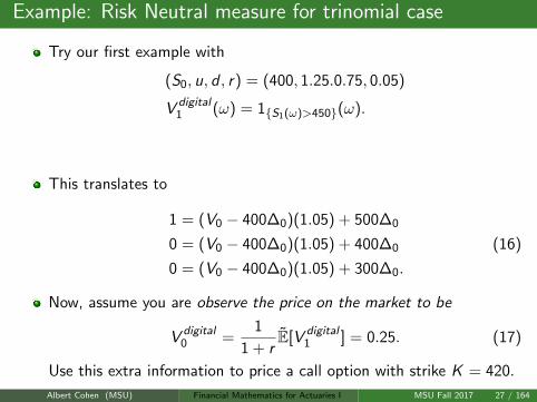
Example: Risk Neutral measure for trinomial case
Try our first example with
(S0, u, d , r) = (400, 1.25.0.75, 0.05)
V digital1 (ω) = 1S1(ω)>450(ω).
This translates to
1 = (V0 − 400∆0)(1.05) + 500∆0
0 = (V0 − 400∆0)(1.05) + 400∆0
0 = (V0 − 400∆0)(1.05) + 300∆0.
(16)
Now, assume you are observe the price on the market to be
V digital0 =
1
1 + rE[V digital
1 ] = 0.25. (17)
Use this extra information to price a call option with strike K = 420.
Albert Cohen (MSU) Financial Mathematics for Actuaries I MSU Fall 2017 27 / 164
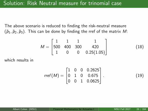
Solution: Risk Neutral measure for trinomial case
The above scenario is reduced to finding the risk-neutral measure(p1, p2, p3). This can be done by finding the rref of the matrix M:
M =
1 1 1 1500 400 300 420
1 0 0 0.25(1.05)
(18)
which results in
rref (M) =
1 0 0 0.26250 1 0 0.6750 0 1 0.0625
. (19)
Albert Cohen (MSU) Financial Mathematics for Actuaries I MSU Fall 2017 28 / 164
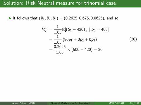
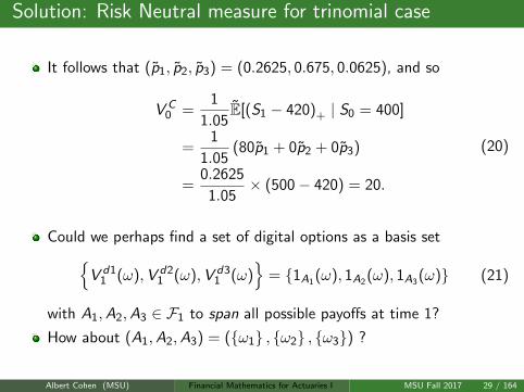
Solution: Risk Neutral measure for trinomial case
It follows that (p1, p2, p3) = (0.2625, 0.675, 0.0625), and so
V C0 =
1
1.05E[(S1 − 420)+ | S0 = 400]
=1
1.05(80p1 + 0p2 + 0p3)
=0.2625
1.05× (500− 420) = 20.
(20)
Could we perhaps find a set of digital options as a basis setV d1
1 (ω),V d21 (ω),V d3
1 (ω)
= 1A1(ω), 1A2(ω), 1A3(ω) (21)
with A1,A2,A3 ∈ F1 to span all possible payoffs at time 1?
How about (A1,A2,A3) = (ω1 , ω2 , ω3) ?
Albert Cohen (MSU) Financial Mathematics for Actuaries I MSU Fall 2017 29 / 164
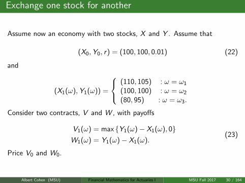
Exchange one stock for another
Assume now an economy with two stocks, X and Y . Assume that
(X0,Y0, r) = (100, 100, 0.01) (22)
and
(X1(ω),Y1(ω)) =
(110, 105) : ω = ω1
(100, 100) : ω = ω2
(80, 95) : ω = ω3.
Consider two contracts, V and W , with payoffs
V1(ω) = max Y1(ω)− X1(ω), 0W1(ω) = Y1(ω)− X1(ω).
(23)
Price V0 and W0.
Albert Cohen (MSU) Financial Mathematics for Actuaries I MSU Fall 2017 30 / 164
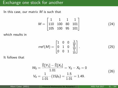
Exchange one stock for another
In this case, our matrix M is such that
M =
1 1 1 1110 100 80 101105 100 95 101
(24)
which results in
rref (M) =
1 0 0 310
0 1 0 610
0 0 1 110
. (25)
It follows that
W0 =E[Y1]− E[X1]
1.01= Y0 − X0 = 0
V0 =1
1.01· (15p3) =
1.5
1.01= 1.49.
(26)
Albert Cohen (MSU) Financial Mathematics for Actuaries I MSU Fall 2017 31 / 164

Homework
From Finan:
Problems 14.1, 14.3, 14.4, 14.5, 14.6, 14.7, 14.11
Problems 15.1, 15.3, 15.4, 15.6, 15.7, 15.10, 15.11
Albert Cohen (MSU) Financial Mathematics for Actuaries I MSU Fall 2017 32 / 164

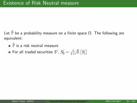
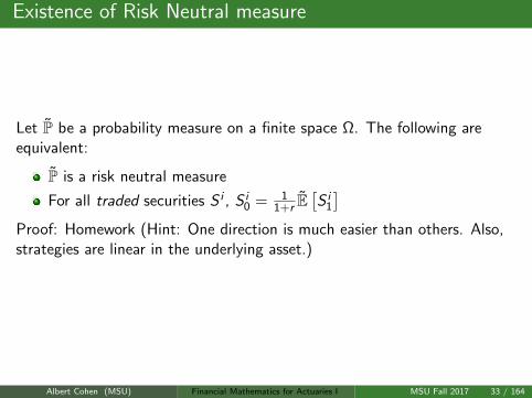
Existence of Risk Neutral measure
Let P be a probability measure on a finite space Ω. The following areequivalent:
P is a risk neutral measure
For all traded securities S i , S i0 = 1
1+r E[S i
1
]Proof: Homework (Hint: One direction is much easier than others. Also,strategies are linear in the underlying asset.)
Albert Cohen (MSU) Financial Mathematics for Actuaries I MSU Fall 2017 33 / 164
Existence of Risk Neutral measure
Let P be a probability measure on a finite space Ω. The following areequivalent:
P is a risk neutral measure
For all traded securities S i , S i0 = 1
1+r E[S i
1
]
Proof: Homework (Hint: One direction is much easier than others. Also,strategies are linear in the underlying asset.)
Albert Cohen (MSU) Financial Mathematics for Actuaries I MSU Fall 2017 33 / 164
Existence of Risk Neutral measure
Let P be a probability measure on a finite space Ω. The following areequivalent:
P is a risk neutral measure
For all traded securities S i , S i0 = 1
1+r E[S i
1
]Proof: Homework (Hint: One direction is much easier than others. Also,strategies are linear in the underlying asset.)
Albert Cohen (MSU) Financial Mathematics for Actuaries I MSU Fall 2017 33 / 164

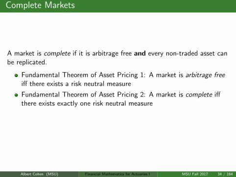
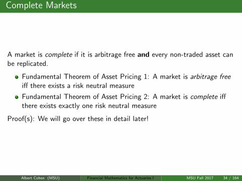
Complete Markets
A market is complete if it is arbitrage free and every non-traded asset canbe replicated.
Fundamental Theorem of Asset Pricing 1: A market is arbitrage freeiff there exists a risk neutral measure
Fundamental Theorem of Asset Pricing 2: A market is complete iffthere exists exactly one risk neutral measure
Proof(s): We will go over these in detail later!
Albert Cohen (MSU) Financial Mathematics for Actuaries I MSU Fall 2017 34 / 164
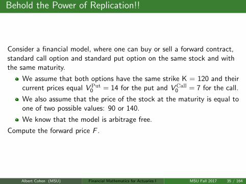
Behold the Power of Replication!!
Consider a financial model, where one can buy or sell a forward contract,standard call option and standard put option on the same stock and withthe same maturity.
We assume that both options have the same strike K = 120 and theircurrent prices equal V Put
0 = 14 for the put and V Call0 = 7 for the call.
We also assume that the price of the stock at the maturity is equal toone of two possible values: 90 or 140.
We know that the model is arbitrage free.
Compute the forward price F .
Albert Cohen (MSU) Financial Mathematics for Actuaries I MSU Fall 2017 35 / 164
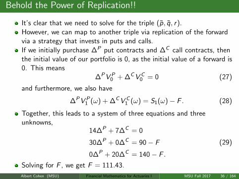
Behold the Power of Replication!!
It’s clear that we need to solve for the triple (p, q, r).
However, we can map to another triple via replication of the forwardvia a strategy that invests in puts and calls.
If we initially purchase ∆P put contracts and ∆C call contracts, thenthe initial value of our portfolio is 0, as the initial value of a forward is0. This means
∆PV P0 + ∆CV C
0 = 0 (27)
and furthermore, we also have
∆PV P1 (ω) + ∆CV C
1 (ω) = S1(ω)− F . (28)
Together, this leads to a system of three equations and threeunknowns,
14∆P + 7∆C = 0
30∆P + 0∆C = 90− F
0∆P + 20∆C = 140− F .
(29)
Solving for F , we get F = 111.43.
Albert Cohen (MSU) Financial Mathematics for Actuaries I MSU Fall 2017 36 / 164
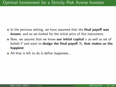
Optimal Investment for a Strictly Risk Averse Investor
In the previous setting, we have assumed that the final payoff wasknown, and so we looked for the initial price of this instrument.
Now, we assume that we know our initial capital x as well as set ofbeliefs P and want to design the final payoff X1 that makes us thehappiest
All that is left to do is define happiness...
Albert Cohen (MSU) Financial Mathematics for Actuaries I MSU Fall 2017 37 / 164
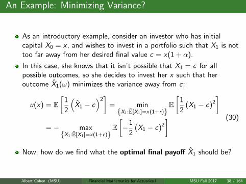
An Example: Minimizing Variance?
As an introductory example, consider an investor who has initialcapital X0 = x , and wishes to invest in a portfolio such that X1 is nottoo far away from her desired final value c = x(1 + α).
In this case, she knows that it isn’t possible that X1 = c for allpossible outcomes, so she decides to invest her x such that heroutcome X1(ω) minimizes the variance away from c :
u(x) = E[
1
2
(X1 − c
)2]
= minX1:E[X1]=x(1+r)
E[
1
2(X1 − c)2
]= − maxX1:E[X1]=x(1+r)
E[−1
2(X1 − c)2
] (30)
Now, how do we find what the optimal final payoff X1 should be?
Albert Cohen (MSU) Financial Mathematics for Actuaries I MSU Fall 2017 38 / 164
Optimal Investment for a Strictly Risk Averse Investor
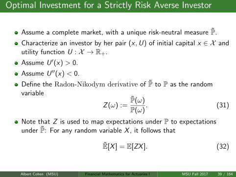
Assume a complete market, with a unique risk-neutral measure P.
Characterize an investor by her pair (x ,U) of initial capital x ∈ X andutility function U : X → R+.
Assume U ′(x) > 0.
Assume U ′′(x) < 0.
Define the Radon-Nikodym derivative of P to P as the randomvariable
Z (ω) :=P(ω)
P(ω). (31)
Note that Z is used to map expectations under P to expectationsunder P: For any random variable X , it follows that
E[X ] = E[ZX ]. (32)
Albert Cohen (MSU) Financial Mathematics for Actuaries I MSU Fall 2017 39 / 164
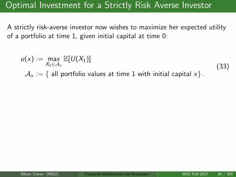
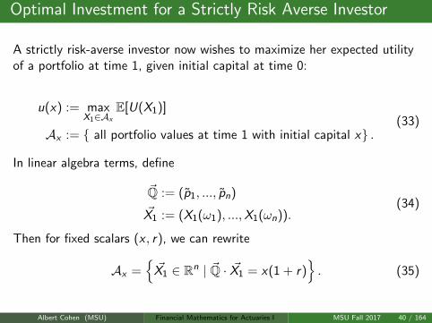
Optimal Investment for a Strictly Risk Averse Investor
A strictly risk-averse investor now wishes to maximize her expected utilityof a portfolio at time 1, given initial capital at time 0:
u(x) := maxX1∈Ax
E[U(X1)]
Ax := all portfolio values at time 1 with initial capital x .(33)
In linear algebra terms, define
~Q := (p1, ..., pn)
~X1 := (X1(ω1), ...,X1(ωn)).(34)
Then for fixed scalars (x , r), we can rewrite
Ax =~X1 ∈ Rn | ~Q · ~X1 = x(1 + r)
. (35)
Albert Cohen (MSU) Financial Mathematics for Actuaries I MSU Fall 2017 40 / 164
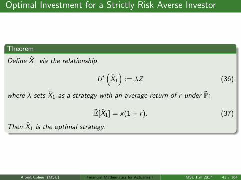
Optimal Investment for a Strictly Risk Averse Investor
Theorem
Define X1 via the relationship
U ′(
X1
):= λZ (36)
where λ sets X1 as a strategy with an average return of r under P:
E[X1] = x(1 + r). (37)
Then X1 is the optimal strategy.
Albert Cohen (MSU) Financial Mathematics for Actuaries I MSU Fall 2017 41 / 164
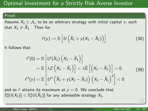
Optimal Investment for a Strictly Risk Averse Investor
Proof.
Assume X1 ∈ Ax to be an arbitrary strategy with initial capital x , suchthat X1 6= X1 . Then for
f (y) := E[U(
X1 + y(X1 − X1))]
(38)
it follows that
f ′(0) = E[U ′(X1)
(X1 − X1
)]= E
[λZ(
X1 − X1
)]= λE
[(X1 − X1
)]= 0
f ′′(y) = E[
U ′′(
X1 + y(X1 − X1))(
X1 − X1
)2]< 0
(39)
and so f attains its maximum at y = 0. We conclude thatE[U(X1)] < E[U(X1)] for any admissible strategy X1.
Albert Cohen (MSU) Financial Mathematics for Actuaries I MSU Fall 2017 42 / 164
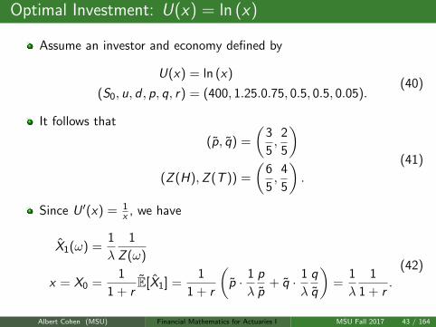
Optimal Investment: U(x) = ln (x)
Assume an investor and economy defined by
U(x) = ln (x)
(S0, u, d , p, q, r) = (400, 1.25.0.75, 0.5, 0.5, 0.05).(40)
It follows that
(p, q) =
(3
5,
2
5
)(Z (H),Z (T )) =
(6
5,
4
5
).
(41)
Since U ′(x) = 1x , we have
X1(ω) =1
λ
1
Z (ω)
x = X0 =1
1 + rE[X1] =
1
1 + r
(p · 1
λ
p
p+ q · 1
λ
q
q
)=
1
λ
1
1 + r.
(42)
Albert Cohen (MSU) Financial Mathematics for Actuaries I MSU Fall 2017 43 / 164
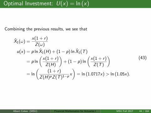
Optimal Investment: U(x) = ln (x)
Combining the previous results, we see that
X1(ω) =x(1 + r)
Z (ω)
u(x) = p ln X1(H) + (1− p) ln X1(T )
= p ln
(x(1 + r)
Z (H)
)+ (1− p) ln
(x(1 + r)
Z (T )
)= ln
((1 + r)
Z (H)pZ (T )1−p x
)= ln (1.0717x) > ln (1.05x).
(43)
Albert Cohen (MSU) Financial Mathematics for Actuaries I MSU Fall 2017 44 / 164
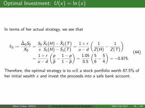
Optimal Investment: U(x) = ln (x)
In terms of her actual strategy, we see that
π0 :=∆0S0
X0=
S0
x
X1(H)− X1(T )
S1(H)− S1(T )=
1 + r
u − d
(1
Z (H)− 1
Z (T )
)=
1 + r
u − d
(p
p− 1− p
1− p
)=
1.05
0.5
(5
6− 5
4
)= −0.875.
(44)
Therefore, the optimal strategy is to sell a stock portfolio worth 87.5% ofher initial wealth x and invest the proceeds into a safe bank account.
Albert Cohen (MSU) Financial Mathematics for Actuaries I MSU Fall 2017 45 / 164
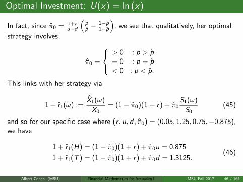
Optimal Investment: U(x) = ln (x)
In fact, since π0 = 1+ru−d
(pp −
1−p1−p
), we see that qualitatively, her optimal
strategy involves
π0 =
> 0 : p > p= 0 : p = p< 0 : p < p.
This links with her strategy via
1 + r1(ω) :=X1(ω)
X0= (1− π0)(1 + r) + π0
S1(ω)
S0(45)
and so for our specific case where (r , u, d , π0) = (0.05, 1.25, 0.75,−0.875),we have
1 + r1(H) = (1− π0)(1 + r) + π0u = 0.875
1 + r1(T ) = (1− π0)(1 + r) + π0d = 1.3125.(46)
Albert Cohen (MSU) Financial Mathematics for Actuaries I MSU Fall 2017 46 / 164
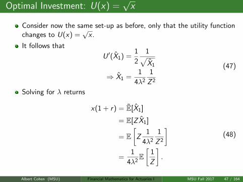
Optimal Investment: U(x) =√x
Consider now the same set-up as before, only that the utility functionchanges to U(x) =
√x .
It follows that
U ′(X1) =1
2
1√X1
⇒ X1 =1
4λ2
1
Z 2
(47)
Solving for λ returns
x(1 + r) = E[X1]
= E[Z X1]
= E[
Z1
4λ2
1
Z 2
]=
1
4λ2E[
1
Z
].
(48)
Albert Cohen (MSU) Financial Mathematics for Actuaries I MSU Fall 2017 47 / 164
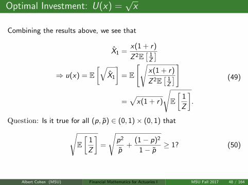
Optimal Investment: U(x) =√x
Combining the results above, we see that
X1 =x(1 + r)
Z 2E[
1Z
]⇒ u(x) = E
[√X1
]= E
[√x(1 + r)
Z 2E[
1Z
]]
=√
x(1 + r)
√E[
1
Z
].
(49)
Question: Is it true for all (p, p) ∈ (0, 1)× (0, 1) that√E[
1
Z
]=
√p2
p+
(1− p)2
1− p≥ 1? (50)
Albert Cohen (MSU) Financial Mathematics for Actuaries I MSU Fall 2017 48 / 164
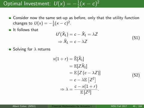
Optimal Investment: U(x) = −12(x − c)2
Consider now the same set-up as before, only that the utility functionchanges to U(x) = −1
2 (x − c)2.
It follows thatU ′(X1) = c − X1 = λZ
⇒ X1 = c − λZ(51)
Solving for λ returns
x(1 + r) = E[X1]
= E[Z X1]
= E [Z (c − λZ )]
= c − λE[Z 2]
⇒ λ =c − x(1 + r)
E [Z 2].
(52)
Albert Cohen (MSU) Financial Mathematics for Actuaries I MSU Fall 2017 49 / 164
Optimal Investment: U(x) = −12(x − c)2
Combining the results above, we see that
X1 = c − c − x(1 + r)
E [Z 2]Z
⇒ u(x) = −E[−1
2
(X1 − c
)2]
= E
[1
2
(c − x(1 + r)
E [Z 2]Z
)2]
=1
2
[c − x(1 + r)2
]=
1
2x2(α− r)2.
(53)
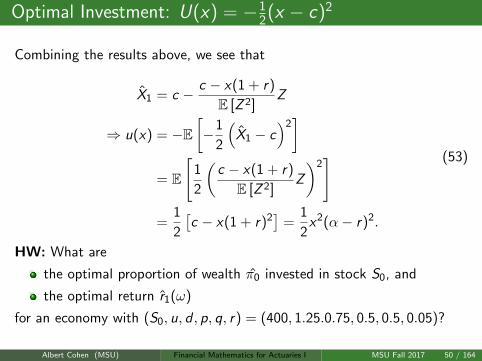
HW: What are
the optimal proportion of wealth π0 invested in stock S0, and
the optimal return r1(ω)
for an economy with (S0, u, d , p, q, r) = (400, 1.25.0.75, 0.5, 0.5, 0.05)?
Albert Cohen (MSU) Financial Mathematics for Actuaries I MSU Fall 2017 50 / 164
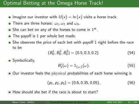
Optimal Betting at the Omega Horse Track!
Imagine our investor with U(x) = ln (x) visits a horse track.
There are three horses: ω1, ω2 and ω3.
She can bet on any of the horses to come in 1st .
The payoff is 1 per whole bet made.
She observes the price of each bet with payoff 1 right before the raceto be
(B10 ,B
20 ,B
30 ) = (0.5, 0.3, 0.2). (54)
Symbolically,B i
1(ω) = 1ωi(ω). (55)
Our investor feels the physical probabilities of each horse winning is
(p1, p2, p3) = (0.6, 0.35, 0.05). (56)
How should she bet if the race is about to start?
Albert Cohen (MSU) Financial Mathematics for Actuaries I MSU Fall 2017 51 / 164
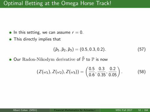
Optimal Betting at the Omega Horse Track!
In this setting, we can assume r = 0.
This directly implies that
(p1, p2, p3) = (0.5, 0.3, 0.2). (57)
Our Radon-Nikodym derivative of P to P is now
(Z (ω1),Z (ω2),Z (ω3)) =
(0.5
0.6,
0.3
0.35,
0.2
0.05
). (58)
Albert Cohen (MSU) Financial Mathematics for Actuaries I MSU Fall 2017 52 / 164
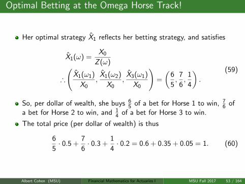
Optimal Betting at the Omega Horse Track!
Her optimal strategy X1 reflects her betting strategy, and satisfies
X1(ω) =X0
Z (ω)
∴
(X1(ω1)
X0,
X1(ω2)
X0,
X3(ω1)
X0
)=
(6
5,
7
6,
1
4
).
(59)
So, per dollar of wealth, she buys 65 of a bet for Horse 1 to win, 7
6 ofa bet for Horse 2 to win, and 1
4 of a bet for Horse 3 to win.
The total price (per dollar of wealth) is thus
6
5· 0.5 +
7
6· 0.3 +
1
4· 0.2 = 0.6 + 0.35 + 0.05 = 1. (60)
Albert Cohen (MSU) Financial Mathematics for Actuaries I MSU Fall 2017 53 / 164
Dividends
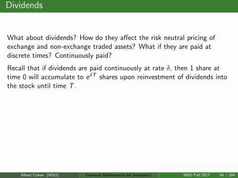
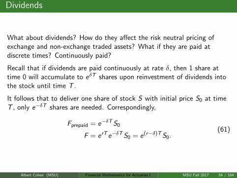
What about dividends? How do they affect the risk neutral pricing ofexchange and non-exchange traded assets? What if they are paid atdiscrete times? Continuously paid?
Recall that if dividends are paid continuously at rate δ, then 1 share attime 0 will accumulate to eδT shares upon reinvestment of dividends intothe stock until time T .
It follows that to deliver one share of stock S with initial price S0 at timeT , only e−δT shares are needed. Correspondingly,
Fprepaid = e−δTS0
F = erT e−δTS0 = e(r−δ)TS0.(61)
Albert Cohen (MSU) Financial Mathematics for Actuaries I MSU Fall 2017 54 / 164
Dividends
What about dividends? How do they affect the risk neutral pricing ofexchange and non-exchange traded assets? What if they are paid atdiscrete times? Continuously paid?
Recall that if dividends are paid continuously at rate δ, then 1 share attime 0 will accumulate to eδT shares upon reinvestment of dividends intothe stock until time T .
It follows that to deliver one share of stock S with initial price S0 at timeT , only e−δT shares are needed. Correspondingly,
Fprepaid = e−δTS0
F = erT e−δTS0 = e(r−δ)TS0.(61)
Albert Cohen (MSU) Financial Mathematics for Actuaries I MSU Fall 2017 54 / 164
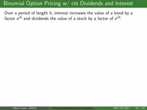
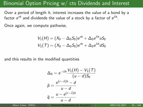
Binomial Option Pricing w/ cts Dividends and Interest
Over a period of length h, interest increases the value of a bond by afactor erh and dividends the value of a stock by a factor of eδh.
Once again, we compute pathwise,
V1(H) = (X0 −∆0S0)erh + ∆0eδhuS0
V1(T ) = (X0 −∆0S0)erh + ∆0eδhdS0
and this results in the modified quantities
∆0 = e−δhV1(H)− V1(T )
(u − d)S0
p =e(r−δ)h − d
u − d
q =u − e(r−δ)h
u − d
Albert Cohen (MSU) Financial Mathematics for Actuaries I MSU Fall 2017 55 / 164
Binomial Option Pricing w/ cts Dividends and Interest
Over a period of length h, interest increases the value of a bond by afactor erh and dividends the value of a stock by a factor of eδh.
Once again, we compute pathwise,
V1(H) = (X0 −∆0S0)erh + ∆0eδhuS0
V1(T ) = (X0 −∆0S0)erh + ∆0eδhdS0
and this results in the modified quantities
∆0 = e−δhV1(H)− V1(T )
(u − d)S0
p =e(r−δ)h − d
u − d
q =u − e(r−δ)h
u − dAlbert Cohen (MSU) Financial Mathematics for Actuaries I MSU Fall 2017 55 / 164
Binomial Models w/ cts Dividends and Interest
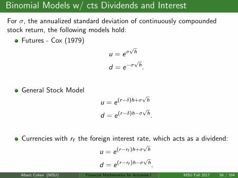
For σ, the annualized standard deviation of continuously compoundedstock return, the following models hold:
Futures - Cox (1979)
u = eσ√h
d = e−σ√h.
General Stock Model
u = e(r−δ)h+σ√h
d = e(r−δ)h−σ√h.
Currencies with rf the foreign interest rate, which acts as a dividend:
u = e(r−rf )h+σ√h
d = e(r−rf )h−σ√h.
Albert Cohen (MSU) Financial Mathematics for Actuaries I MSU Fall 2017 56 / 164

1- and 2-period pricing
We can solve for 2-period problems
on a case-by-case basis, or
by developing a general theory for multi-period asset pricing.
In the latter method, we need a general framework to carry out ourcomputations
Albert Cohen (MSU) Financial Mathematics for Actuaries I MSU Fall 2017 57 / 164
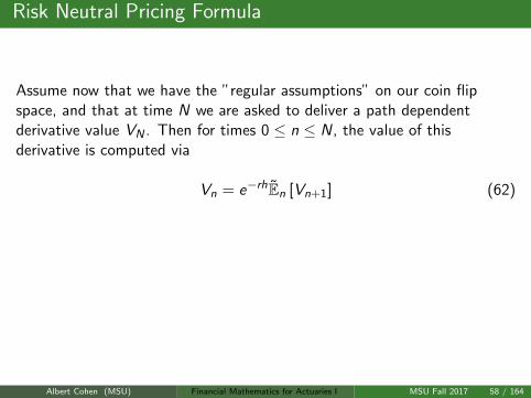
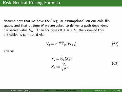
Risk Neutral Pricing Formula
Assume now that we have the ”regular assumptions” on our coin flipspace, and that at time N we are asked to deliver a path dependentderivative value VN . Then for times 0 ≤ n ≤ N, the value of thisderivative is computed via
Vn = e−rhEn [Vn+1] (62)
and so
X0 = E0 [XN ]
Xn :=Vn
enh.
(63)
Albert Cohen (MSU) Financial Mathematics for Actuaries I MSU Fall 2017 58 / 164
Computational Complexity
Consider the case
p = q =1
2
S0 = 4, u =4
3, d =
3
4
(64)
but now with term n = 3.
There are 23 = 8 paths to consider.
However, there are 3 + 1 = 4 unique final values of S3 to consider.
In the general term N, there would be 2N paths to generate SN , butonly N + 1 distinct values.
At any node n units of time into the asset’s evolution, there are n + 1distinct values.
Albert Cohen (MSU) Financial Mathematics for Actuaries I MSU Fall 2017 59 / 164
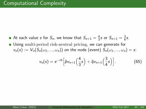
Computational Complexity
At each value s for Sn, we know that Sn+1 = 43 s or Sn+1 = 3
4 s.
Using multi-period risk-neutral pricing, we can generate forvn(s) := Vn(Sn(ω1, ..., ωn)) on the node (event) Sn(ω1, ..., ωn) = s:
vn(s) = e−rh[pvn+1
(4
3s)
+ qvn+1
(3
4s)]. (65)
Albert Cohen (MSU) Financial Mathematics for Actuaries I MSU Fall 2017 60 / 164
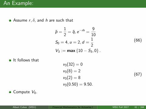
An Example:
Assume r , δ, and h are such that
p =1
2= q, e−rh =
9
10
S0 = 4, u = 2, d =1
2V3 := max 10− S3, 0 .
(66)
It follows thatv3(32) = 0
v3(8) = 2
v3(2) = 8
v3(0.50) = 9.50.
(67)
Compute V0.
Albert Cohen (MSU) Financial Mathematics for Actuaries I MSU Fall 2017 61 / 164
Another Example
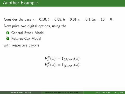
Consider the case r = 0.10, δ = 0.05, h = 0.01, σ = 0.1,S0 = 10 = K .
Now price two digital options, using the
1 General Stock Model
2 Futures-Cox Model
with respective payoffs
V K1 (ω) := 1S1≥K(ω)
V K2 (ω) := 1S2≥K(ω).
Albert Cohen (MSU) Financial Mathematics for Actuaries I MSU Fall 2017 62 / 164
Another Example
Consider the case r = 0.10, δ = 0.05, h = 0.01, σ = 0.1,S0 = 10 = K .
Now price two digital options, using the
1 General Stock Model
2 Futures-Cox Model
with respective payoffs
V K1 (ω) := 1S1≥K(ω)
V K2 (ω) := 1S2≥K(ω).
Albert Cohen (MSU) Financial Mathematics for Actuaries I MSU Fall 2017 62 / 164
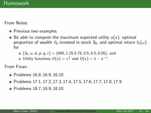
Homework
From Notes:
Previous two examples.
Be able to compute the maximum expected utility u(x), optimalproportion of wealth π0 invested in stock S0, and optimal return r1(ω)for
(S0, u, d , p, q, r) = (400, 1.25.0.75, 0.5, 0.5, 0.05), and
Utility functions U(x) = x13 and U(x) = 1− e−x .
From Finan:
Problems 16.8, 16.9, 16.10
Problems 17.1, 17.2, 17.3, 17.4, 17.5, 17.6, 17.7, 17.8, 17.9
Problems 18.7, 18.9, 18.10.
Albert Cohen (MSU) Financial Mathematics for Actuaries I MSU Fall 2017 63 / 164
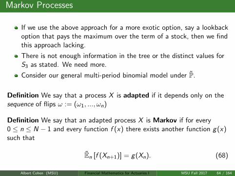
Markov Processes
If we use the above approach for a more exotic option, say a lookbackoption that pays the maximum over the term of a stock, then we findthis approach lacking.
There is not enough information in the tree or the distinct values forS3 as stated. We need more.
Consider our general multi-period binomial model under P.
Definition We say that a process X is adapted if it depends only on thesequence of flips ω := (ω1, ..., ωn)
Definition We say that an adapted process X is Markov if for every0 ≤ n ≤ N − 1 and every function f (x) there exists another function g(x)such that
En [f (Xn+1)] = g(Xn). (68)
Albert Cohen (MSU) Financial Mathematics for Actuaries I MSU Fall 2017 64 / 164
Markov Processes
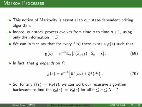
This notion of Markovity is essential to our state-dependent pricingalgorithm.
Indeed, our stock process evolves from time n to time n + 1, usingonly the information in Sn.
We can in fact say that for every f (s) there exists a g(s) such that
g(s) = e−rhEn [f (Sn+1) | Sn = s] . (69)
In fact, that g depends on f :
g(s) = e−rh[pf (us) + qf (ds)
]. (70)
So, for any f (s) := VN(s), we can work our recursive algorithmbackwards to find the gn(s) := Vn(s) for all 0 ≤ n ≤ N − 1
Albert Cohen (MSU) Financial Mathematics for Actuaries I MSU Fall 2017 65 / 164
Markov Processes
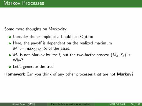
Some more thoughts on Markovity:
Consider the example of a Lookback Option.
Here, the payoff is dependent on the realized maximumMn := max0≤i≤nSi of the asset.
Mn is not Markov by itself, but the two-factor process (Mn, Sn) is.Why?
Let’s generate the tree!
Homework Can you think of any other processes that are not Markov?
Albert Cohen (MSU) Financial Mathematics for Actuaries I MSU Fall 2017 66 / 164
The Interview Process
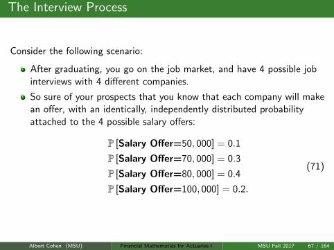
Consider the following scenario:
After graduating, you go on the job market, and have 4 possible jobinterviews with 4 different companies.
So sure of your prospects that you know that each company will makean offer, with an identically, independently distributed probabilityattached to the 4 possible salary offers:
P [Salary Offer=50, 000] = 0.1
P [Salary Offer=70, 000] = 0.3
P [Salary Offer=80, 000] = 0.4
P [Salary Offer=100, 000] = 0.2.
(71)
Albert Cohen (MSU) Financial Mathematics for Actuaries I MSU Fall 2017 67 / 164

The Interview Process
Questions:
How should you interview?
Specifically, when should you accept an offer and cancel theremaining interviews?
How does your strategy change if you can interview as many times asyou like, but the distribution of offers remains the same as above?
Albert Cohen (MSU) Financial Mathematics for Actuaries I MSU Fall 2017 68 / 164

The Interview Process: Strategy
Some more thoughts...
At any time the student will know only one offer, which she can eitheraccept or reject.
Of course, if the student rejects the first three offers, than she has toaccept the last one.
So, compute the maximal expected salary for the student after thegraduation and the corresponding optimal strategy.
Albert Cohen (MSU) Financial Mathematics for Actuaries I MSU Fall 2017 69 / 164
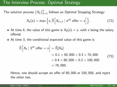
The Interview Process: Optimal Strategy
The solution process Xk4k=1 follows an Optimal Stopping Strategy:
Xk(s) = max
s, E[Xk+1 | kth offer = s
]. (72)
At time 4, the value of this game is X4(s) = s, with s being the salaryoffered.
At time 3, the conditional expected value of this game is
E[X4 | 3rd offer = s
]= E[X4]
= 0.1× 50, 000 + 0.3× 70, 000
+ 0.4× 80, 000 + 0.2× 100, 000
= 78, 000.
(73)
Hence, one should accept an offer of 80, 000 or 100, 000, and rejectthe other two.
Albert Cohen (MSU) Financial Mathematics for Actuaries I MSU Fall 2017 70 / 164
The Interview Process: Optimal Strategy
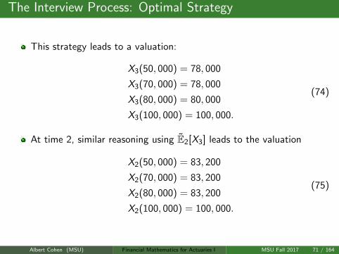
This strategy leads to a valuation:
X3(50, 000) = 78, 000
X3(70, 000) = 78, 000
X3(80, 000) = 80, 000
X3(100, 000) = 100, 000.
(74)
At time 2, similar reasoning using E2[X3] leads to the valuation
X2(50, 000) = 83, 200
X2(70, 000) = 83, 200
X2(80, 000) = 83, 200
X2(100, 000) = 100, 000.
(75)
Albert Cohen (MSU) Financial Mathematics for Actuaries I MSU Fall 2017 71 / 164
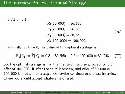
The Interview Process: Optimal Strategy
At time 1,X1(50, 000) = 86, 560
X1(70, 000) = 86, 560
X1(80, 000) = 86, 560
X1(100, 000) = 100, 000.
(76)
Finally, at time 0, the value of this optimal strategy is
E0[X1] = E[X1] = 0.8× 86, 560 + 0.2× 100, 000 = 89, 248. (77)
So, the optimal strategy is, for the first two interviews, accept only anoffer of 100, 000. If after the third interview, and offer of 80, 000 or100, 000 is made, then accept. Otherwise continue to the last interviewwhere you should accept whatever is offered.
Albert Cohen (MSU) Financial Mathematics for Actuaries I MSU Fall 2017 72 / 164

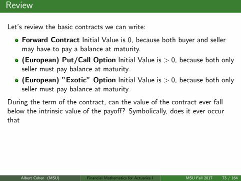
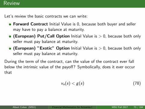
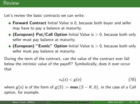
Review
Let’s review the basic contracts we can write:
Forward Contract Initial Value is 0, because both buyer and sellermay have to pay a balance at maturity.
(European) Put/Call Option Initial Value is > 0, because both onlyseller must pay balance at maturity.
(European) ”Exotic” Option Initial Value is > 0, because both onlyseller must pay balance at maturity.
During the term of the contract, can the value of the contract ever fallbelow the intrinsic value of the payoff? Symbolically, does it ever occurthat
vn(s) < g(s) (78)
where g(s) is of the form of g(S) := max S − K , 0, in the case of a Calloption, for example.
Albert Cohen (MSU) Financial Mathematics for Actuaries I MSU Fall 2017 73 / 164

For Freedom! (we must charge extra...)
What happens if we write a contract that allows the purchaser to exercisethe contract whenever she feels it to be in her advantage? By allowing thisextra freedom, we must
Charge more than we would for a European contract that is exercisedonly at the term N.
Hedge our replicating strategy X differently, to allow for thepossibility of early exercise.
Albert Cohen (MSU) Financial Mathematics for Actuaries I MSU Fall 2017 74 / 164
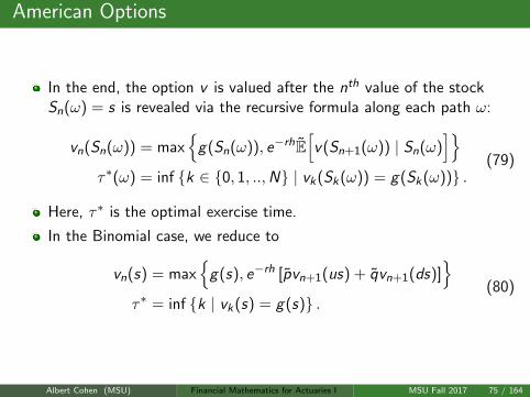
American Options
In the end, the option v is valued after the nth value of the stockSn(ω) = s is revealed via the recursive formula along each path ω:
vn(Sn(ω)) = max
g(Sn(ω)), e−rhE[v(Sn+1(ω)) | Sn(ω)
]τ∗(ω) = inf k ∈ 0, 1, ..,N | vk(Sk(ω)) = g(Sk(ω)) .
(79)
Here, τ∗ is the optimal exercise time.
In the Binomial case, we reduce to
vn(s) = max
g(s), e−rh [pvn+1(us) + qvn+1(ds)]
τ∗ = inf k | vk(s) = g(s) .(80)
Albert Cohen (MSU) Financial Mathematics for Actuaries I MSU Fall 2017 75 / 164
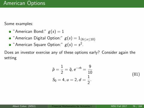
American Options
Some examples:
”American Bond:” g(s) = 1
”American Digital Option:” g(s) = 16≤s≤10
”American Square Option:” g(s) = s2.
Does an investor exercise any of these options early? Consider again thesetting
p =1
2= q, e−rh =
9
10
S0 = 4, u = 2, d =1
2.
(81)
Albert Cohen (MSU) Financial Mathematics for Actuaries I MSU Fall 2017 76 / 164
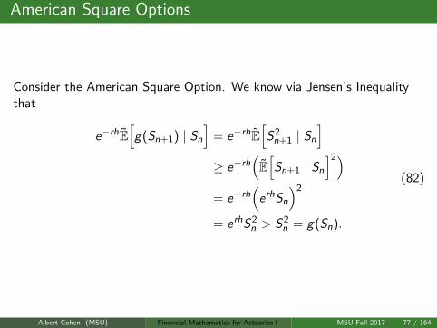
American Square Options
Consider the American Square Option. We know via Jensen’s Inequalitythat
e−rhE[g(Sn+1) | Sn
]= e−rhE
[S2n+1 | Sn
]≥ e−rh
(E[Sn+1 | Sn
]2)= e−rh
(erhSn
)2
= erhS2n > S2
n = g(Sn).
(82)
Albert Cohen (MSU) Financial Mathematics for Actuaries I MSU Fall 2017 77 / 164
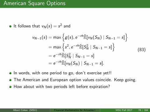
American Square Options
It follows that vN(s) = s2 and
vN−1(s) = max
g(s), e−rhE[vN(SN) | SN−1 = s]
= max
s2, e−rhE[S2N | SN−1 = s]
= e−rhE[S2
N | SN−1 = s]
= e−rhE[vN(SN) | SN−1 = s].
(83)
In words, with one period to go, don’t exercise yet!!
The American and European option values coincide. Keep going.
How about with two periods left before expiration?
Albert Cohen (MSU) Financial Mathematics for Actuaries I MSU Fall 2017 78 / 164
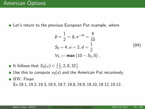
American Options
Let’s return to the previous European Put example, where
p =1
2= q, e−rh =
9
10
S0 = 4, u = 2, d =1
2V3 := max 10− S3, 0 .
(84)
It follows that S3(ω) ∈
12 , 2, 8, 32
.
Use this to compute v3(s) and the American Put recursively.
HW: FinanEx.19.1, 19.2, 19.3, 19.5, 19.7, 19.8, 19.9, 19.10, 19.12, 19.13 .
Albert Cohen (MSU) Financial Mathematics for Actuaries I MSU Fall 2017 79 / 164
Asian Options
In times of high volatility or frequent trading, a company may want toprotect against large price movements over an entire time period, using anaverage. For example, if a company is looking at foreign exchange marketsor markets that may be subject to stock pinning due to large actors.
As an input, the average of an asset is used as an input against a strike,instead of the spot price.
There are two possibilities for the input in the discrete case: h = TN and
Arithmetic Average: IA(T ) := 1N+1
∑Nk=0 Skh .
Geometric Average: IG (T ) :=(
ΠNk=0Skh
) 1N+1
.
HW: Is there an ordering for IA, IG that is independent of T ?
Albert Cohen (MSU) Financial Mathematics for Actuaries I MSU Fall 2017 80 / 164
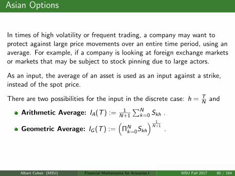
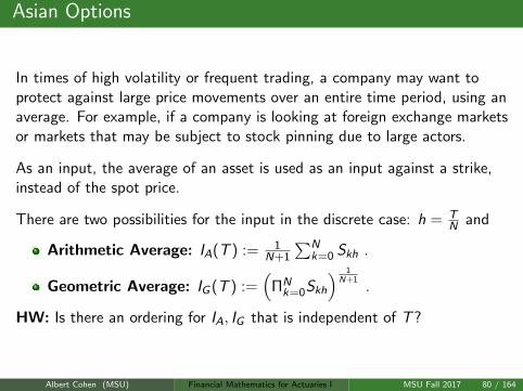
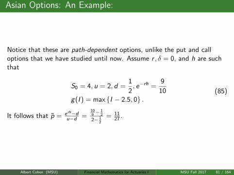
Asian Options: An Example:
Notice that these are path-dependent options, unlike the put and calloptions that we have studied until now. Assume r , δ = 0, and h are suchthat
S0 = 4, u = 2, d =1
2, e−rh =
9
10g(I ) = max I − 2.5, 0 .
(85)
It follows that p = erh−du−d =
109− 1
2
2− 12
= 1127 .
Albert Cohen (MSU) Financial Mathematics for Actuaries I MSU Fall 2017 81 / 164
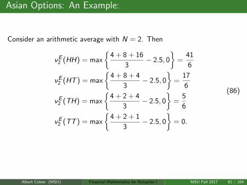
Asian Options: An Example:
Consider an arithmetic average with N = 2. Then
vE2 (HH) = max
4 + 8 + 16
3− 2.5, 0
=
41
6
vE2 (HT ) = max
4 + 8 + 4
3− 2.5, 0
=
17
6
vE2 (TH) = max
4 + 2 + 4
3− 2.5, 0
=
5
6
vE2 (TT ) = max
4 + 2 + 1
3− 2.5, 0
= 0.
(86)
Compute v0, assuming a European structure. How about an Americanstructure?
Albert Cohen (MSU) Financial Mathematics for Actuaries I MSU Fall 2017 82 / 164
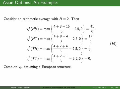
Asian Options: An Example:
Consider an arithmetic average with N = 2. Then
vE2 (HH) = max
4 + 8 + 16
3− 2.5, 0
=
41
6
vE2 (HT ) = max
4 + 8 + 4
3− 2.5, 0
=
17
6
vE2 (TH) = max
4 + 2 + 4
3− 2.5, 0
=
5
6
vE2 (TT ) = max
4 + 2 + 1
3− 2.5, 0
= 0.
(86)
Compute v0, assuming a European structure.
How about an Americanstructure?
Albert Cohen (MSU) Financial Mathematics for Actuaries I MSU Fall 2017 82 / 164
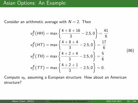
Asian Options: An Example:
Consider an arithmetic average with N = 2. Then
vE2 (HH) = max
4 + 8 + 16
3− 2.5, 0
=
41
6
vE2 (HT ) = max
4 + 8 + 4
3− 2.5, 0
=
17
6
vE2 (TH) = max
4 + 2 + 4
3− 2.5, 0
=
5
6
vE2 (TT ) = max
4 + 2 + 1
3− 2.5, 0
= 0.
(86)
Compute v0, assuming a European structure. How about an Americanstructure?
Albert Cohen (MSU) Financial Mathematics for Actuaries I MSU Fall 2017 82 / 164
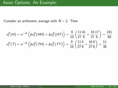
Asian Options: An Example:
Consider an arithmetic average with N = 2. Then
vE1 (H) = e−rh
(pvE
2 (HH) + qvE2 (HT )
)=
9
10
(11
27
41
6+
16
27
17
6
)=
241
60
vE1 (T ) = e−rh
(pvE
2 (TH) + qvE2 (TT )
)=
9
10
(11
27
5
6+
16
27
0
6
)=
11
36
∴ vE0 = e−rh
(pvE
1 (H) + qvE1 (T )
)=
9
10
(11
27
241
60+
16
27
11
36
)=
8833
5400
≈ 1.636.(87)
Albert Cohen (MSU) Financial Mathematics for Actuaries I MSU Fall 2017 83 / 164
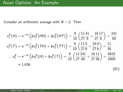
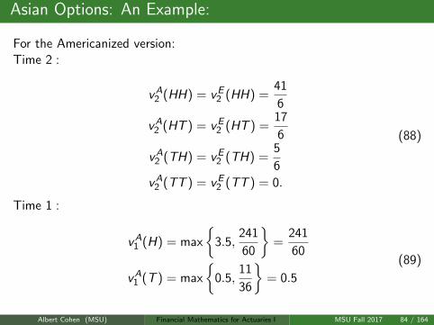
Asian Options: An Example:
For the Americanized version:Time 2 :
vA2 (HH) = vE
2 (HH) =41
6
vA2 (HT ) = vE
2 (HT ) =17
6
vA2 (TH) = vE
2 (TH) =5
6
vA2 (TT ) = vE
2 (TT ) = 0.
(88)
Time 1 :
vA1 (H) = max
3.5,
241
60
=
241
60
vA1 (T ) = max
0.5,
11
36
= 0.5
(89)
Albert Cohen (MSU) Financial Mathematics for Actuaries I MSU Fall 2017 84 / 164
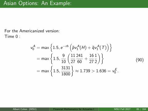
Asian Options: An Example:
For the Americanized version:Time 0 :
vA0 = max
1.5, e−rh
(pvA
1 (H) + qvA1 (T )
)= max
1.5,
9
10
(11
27
241
60+
16
27
1
2
)= max
1.5,
3131
1800
≈ 1.739 > 1.636 = vE
0 .
(90)
Albert Cohen (MSU) Financial Mathematics for Actuaries I MSU Fall 2017 85 / 164
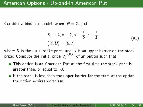
American Options - Up-and-In American Put
Consider a binomial model, where N = 2, and
S0 = 4, u = 2, d =1
2, r =
1
4(K ,U) = (5, 7)
(91)
where K is the usual strike price, and U is an upper barrier on the stockprice. Compute the initial price V A,P,U
0 of an option such that
This option is an American Put at the first time the stock price isgreater than, or equal to, U.
If the stock is less than the upper barrier for the term of the option,the option expires worthless.
Albert Cohen (MSU) Financial Mathematics for Actuaries I MSU Fall 2017 86 / 164
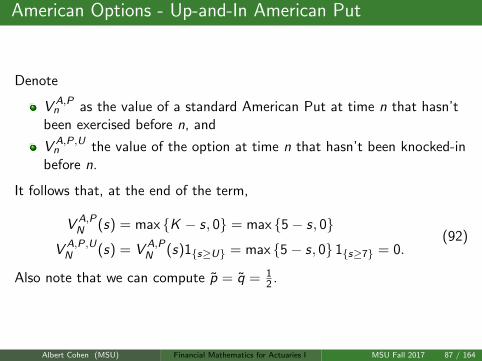
American Options - Up-and-In American Put
Denote
V A,Pn as the value of a standard American Put at time n that hasn’t
been exercised before n, and
V A,P,Un the value of the option at time n that hasn’t been knocked-in
before n.
It follows that, at the end of the term,
V A,PN (s) = max K − s, 0 = max 5− s, 0
V A,P,UN (s) = V A,P
N (s)1s≥U = max 5− s, 0 1s≥7 = 0.(92)
Also note that we can compute p = q = 12 .
Albert Cohen (MSU) Financial Mathematics for Actuaries I MSU Fall 2017 87 / 164
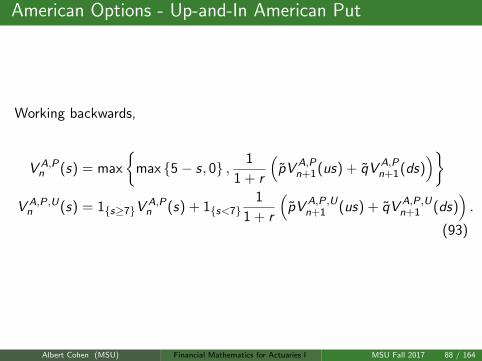
American Options - Up-and-In American Put
Working backwards,
V A,Pn (s) = max
max 5− s, 0 , 1
1 + r
(pV A,P
n+1(us) + qV A,Pn+1(ds)
)V A,P,Un (s) = 1s≥7V
A,Pn (s) + 1s<7
1
1 + r
(pV A,P,U
n+1 (us) + qV A,P,Un+1 (ds)
).
(93)
Albert Cohen (MSU) Financial Mathematics for Actuaries I MSU Fall 2017 88 / 164
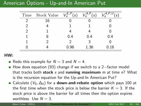
American Options - Up-and-In American Put
Time Stock Value V E ,Pn (s) V A,P
n (s) V A,P,Un (s)
2 16 0 0 02 4 1 1 02 1 4 4 01 8 0.4 0.4 0.41 2 2 3 00 4 0.96 1.36 0.16
HW:
Redo this example for N = 3 and N = 4.How does equation (93) change if we switch to a 2−factor modelthat tracks both stock s and running maximum m at time n? Whatis the recursion equation for the Up-and-In American Put?Calculate (V0,∆0) for a down-and-rebate option which pays 100 atthe first time when the stock price is below the barrier K = 3. If thestock price is above the barrier for all times then the option expiresworthless. Use N = 3.Albert Cohen (MSU) Financial Mathematics for Actuaries I MSU Fall 2017 89 / 164
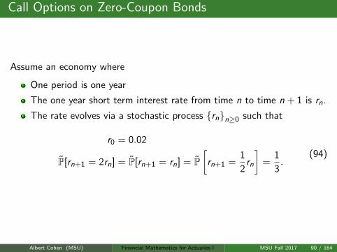
Call Options on Zero-Coupon Bonds
Assume an economy where
One period is one year
The one year short term interest rate from time n to time n + 1 is rn.
The rate evolves via a stochastic process rnn≥0 such that
r0 = 0.02
P[rn+1 = 2rn] = P[rn+1 = rn] = P[
rn+1 =1
2rn
]=
1
3.
(94)
Albert Cohen (MSU) Financial Mathematics for Actuaries I MSU Fall 2017 90 / 164
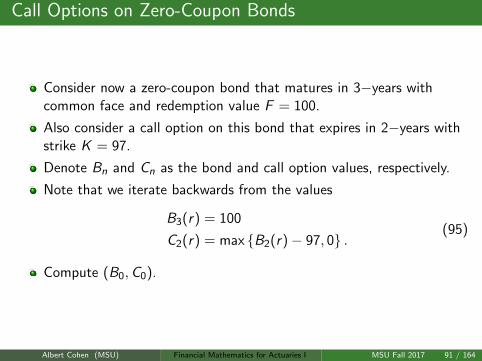
Call Options on Zero-Coupon Bonds
Consider now a zero-coupon bond that matures in 3−years withcommon face and redemption value F = 100.
Also consider a call option on this bond that expires in 2−years withstrike K = 97.
Denote Bn and Cn as the bond and call option values, respectively.
Note that we iterate backwards from the values
B3(r) = 100
C2(r) = max B2(r)− 97, 0 .(95)
Compute (B0,C0).
Albert Cohen (MSU) Financial Mathematics for Actuaries I MSU Fall 2017 91 / 164
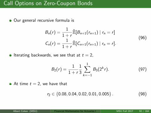
Call Options on Zero-Coupon Bonds
Our general recursive formula is
Bn(r) =1
1 + rE[Bn+1(rn+1) | rn = r ]
Cn(r) =1
1 + rE[Cn+1(rn+1) | rn = r ].
(96)
Iterating backwards, we see that at t = 2,
B2(r) =1
1 + r
1
3
1∑k=−1
B3(2k r). (97)
At time t = 2, we have that
r2 ∈ 0.08, 0.04, 0.02, 0.01, 0.005 . (98)
Albert Cohen (MSU) Financial Mathematics for Actuaries I MSU Fall 2017 92 / 164
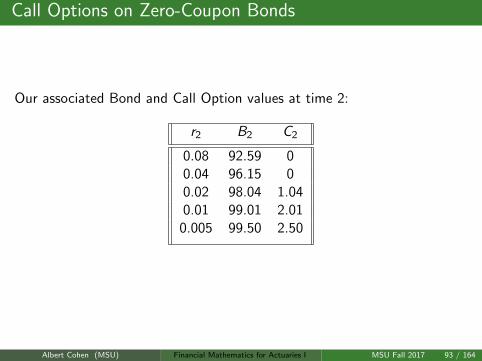
Call Options on Zero-Coupon Bonds
Our associated Bond and Call Option values at time 2:
r2 B2 C2
0.08 92.59 00.04 96.15 00.02 98.04 1.040.01 99.01 2.01
0.005 99.50 2.50
Albert Cohen (MSU) Financial Mathematics for Actuaries I MSU Fall 2017 93 / 164
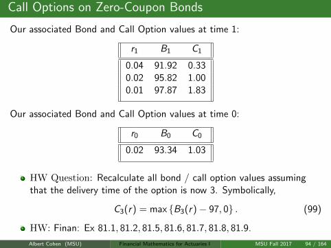
Call Options on Zero-Coupon Bonds
Our associated Bond and Call Option values at time 1:
r1 B1 C1
0.04 91.92 0.330.02 95.82 1.000.01 97.87 1.83
Our associated Bond and Call Option values at time 0:
r0 B0 C0
0.02 93.34 1.03
HW Question: Recalculate all bond / call option values assumingthat the delivery time of the option is now 3. Symbolically,
C3(r) = max B3(r)− 97, 0 . (99)
HW: Finan: Ex 81.1, 81.2, 81.5, 81.6, 81.7, 81.8, 81.9.
Albert Cohen (MSU) Financial Mathematics for Actuaries I MSU Fall 2017 94 / 164
Matching Interest Rates to Market Conditions
Consider again a series of coin flips (ω1, ..., ωn) where at time n, theinterest rate from n to n + 1 is modeled via
rn = rn(ω1, ..., ωn) (100)
Keep in mind that we will build a recombining binomial tree for thismodel. So, for example,
r2(H,T ) = r2(T ,H). (101)
Albert Cohen (MSU) Financial Mathematics for Actuaries I MSU Fall 2017 95 / 164
Matching Interest Rates to Market Conditions
Furthermore, we can define the yield rate y(t,T , r(t)) for a zero-couponbond B(t,T , r(t)) via
B(t,T , r(t)) =1
(1 + y(t,T , r(t)))T−t(102)
Given yield rates, there is also the corresponding yield rate volatility
σn =1
2ln
(y(1, n, r1(H))
y(1, n, r1(T ))
). (103)
We compare the yield rate volatility with the short rate volatility
σn =1
2ln
(rn(ω1, ..., ωn−1, ωn = H)
rn(ω1, ..., ωn−1, ωn = T )
). (104)
Albert Cohen (MSU) Financial Mathematics for Actuaries I MSU Fall 2017 96 / 164
Matching Interest Rates to Market Conditions
We can in fact see that
y(1, 2, r1(H)) = r1(H)
y(1, 2, r1(T )) = r1(T ).(105)
But, for example, it is not clear how to obtain
(y(1, 3, r1(H)), y(1, 3, r1(T ))) . (106)
Furthermore, how can we match to market conditions and update ourestimates for interest rates rn?
Albert Cohen (MSU) Financial Mathematics for Actuaries I MSU Fall 2017 97 / 164
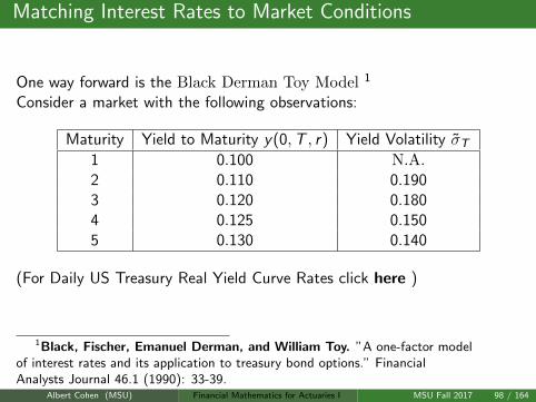
Matching Interest Rates to Market Conditions
One way forward is the Black Derman Toy Model 1
Consider a market with the following observations:
Maturity Yield to Maturity y(0,T , r) Yield Volatility σT1 0.100 N.A.2 0.110 0.1903 0.120 0.1804 0.125 0.1505 0.130 0.140
(For Daily US Treasury Real Yield Curve Rates click here )
1Black, Fischer, Emanuel Derman, and William Toy. ”A one-factor modelof interest rates and its application to treasury bond options.” FinancialAnalysts Journal 46.1 (1990): 33-39.
Albert Cohen (MSU) Financial Mathematics for Actuaries I MSU Fall 2017 98 / 164
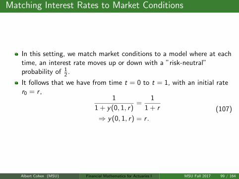
Matching Interest Rates to Market Conditions
In this setting, we match market conditions to a model where at eachtime, an interest rate moves up or down with a ”risk-neutral”probability of 1
2 .
It follows that we have from time t = 0 to t = 1, with an initial rater0 = r ,
1
1 + y(0, 1, r)=
1
1 + r
⇒ y(0, 1, r) = r .
(107)
Albert Cohen (MSU) Financial Mathematics for Actuaries I MSU Fall 2017 99 / 164
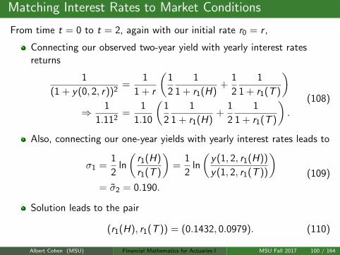
Matching Interest Rates to Market Conditions
From time t = 0 to t = 2, again with our initial rate r0 = r ,
Connecting our observed two-year yield with yearly interest ratesreturns
1
(1 + y(0, 2, r))2=
1
1 + r
(1
2
1
1 + r1(H)+
1
2
1
1 + r1(T )
)⇒ 1
1.112=
1
1.10
(1
2
1
1 + r1(H)+
1
2
1
1 + r1(T )
).
(108)
Also, connecting our one-year yields with yearly interest rates leads to
σ1 =1
2ln
(r1(H)
r1(T )
)=
1
2ln
(y(1, 2, r1(H))
y(1, 2, r1(T ))
)= σ2 = 0.190.
(109)
Solution leads to the pair
(r1(H), r1(T )) = (0.1432, 0.0979). (110)
Albert Cohen (MSU) Financial Mathematics for Actuaries I MSU Fall 2017 100 / 164
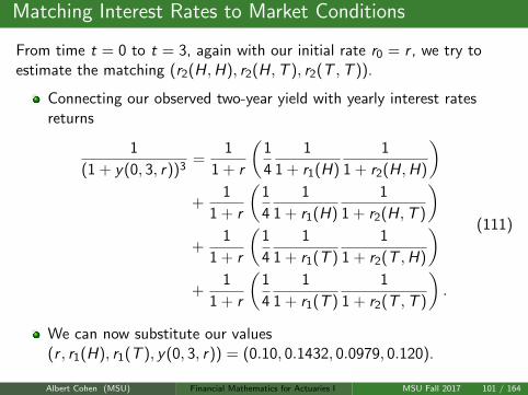
Matching Interest Rates to Market Conditions
From time t = 0 to t = 3, again with our initial rate r0 = r , we try toestimate the matching (r2(H,H), r2(H,T ), r2(T ,T )).
Connecting our observed two-year yield with yearly interest ratesreturns
1
(1 + y(0, 3, r))3=
1
1 + r
(1
4
1
1 + r1(H)
1
1 + r2(H,H)
)+
1
1 + r
(1
4
1
1 + r1(H)
1
1 + r2(H,T )
)+
1
1 + r
(1
4
1
1 + r1(T )
1
1 + r2(T ,H)
)+
1
1 + r
(1
4
1
1 + r1(T )
1
1 + r2(T ,T )
).
(111)
We can now substitute our values(r , r1(H), r1(T ), y(0, 3, r)) = (0.10, 0.1432, 0.0979, 0.120).
Albert Cohen (MSU) Financial Mathematics for Actuaries I MSU Fall 2017 101 / 164
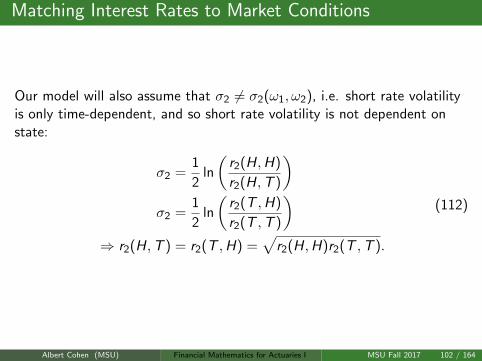
Matching Interest Rates to Market Conditions
Our model will also assume that σ2 6= σ2(ω1, ω2), i.e. short rate volatilityis only time-dependent, and so short rate volatility is not dependent onstate:
σ2 =1
2ln
(r2(H,H)
r2(H,T )
)σ2 =
1
2ln
(r2(T ,H)
r2(T ,T )
)⇒ r2(H,T ) = r2(T ,H) =
√r2(H,H)r2(T ,T ).
(112)
Albert Cohen (MSU) Financial Mathematics for Actuaries I MSU Fall 2017 102 / 164
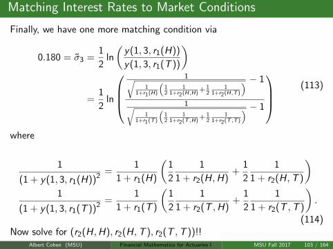
Matching Interest Rates to Market Conditions
Finally, we have one more matching condition via
0.180 = σ3 =1
2ln
(y(1, 3, r1(H))
y(1, 3, r1(T ))
)
=1
2ln
1√
11+r1(H)
(12
11+r2(H,H)
+ 12
11+r2(H,T )
) − 1
1√1
1+r1(T )
(12
11+r2(T ,H)
+ 12
11+r2(T ,T )
) − 1
(113)
where
1
(1 + y(1, 3, r1(H))2=
1
1 + r1(H)
(1
2
1
1 + r2(H,H)+
1
2
1
1 + r2(H,T )
)1
(1 + y(1, 3, r1(T ))2=
1
1 + r1(T )
(1
2
1
1 + r2(T ,H)+
1
2
1
1 + r2(T ,T )
).
(114)Now solve for (r2(H,H), r2(H,T ), r2(T ,T ))!!
Albert Cohen (MSU) Financial Mathematics for Actuaries I MSU Fall 2017 103 / 164
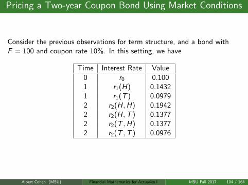
Pricing a Two-year Coupon Bond Using Market Conditions
Consider the previous observations for term structure, and a bond withF = 100 and coupon rate 10%. In this setting, we have
Time Interest Rate Value
0 r0 0.1001 r1(H) 0.14321 r1(T ) 0.09792 r2(H,H) 0.19422 r2(H,T ) 0.13772 r2(T ,H) 0.13772 r2(T ,T ) 0.0976
Albert Cohen (MSU) Financial Mathematics for Actuaries I MSU Fall 2017 104 / 164
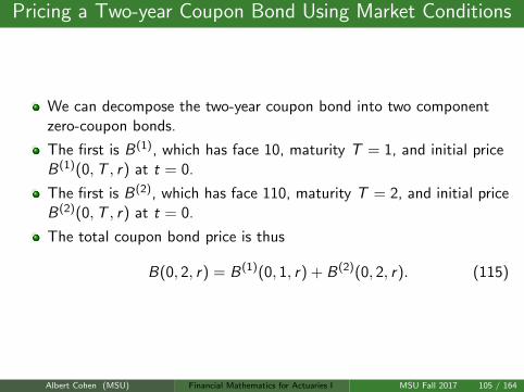
Pricing a Two-year Coupon Bond Using Market Conditions
We can decompose the two-year coupon bond into two componentzero-coupon bonds.
The first is B(1), which has face 10, maturity T = 1, and initial priceB(1)(0,T , r) at t = 0.
The first is B(2), which has face 110, maturity T = 2, and initial priceB(2)(0,T , r) at t = 0.
The total coupon bond price is thus
B(0, 2, r) = B(1)(0, 1, r) + B(2)(0, 2, r). (115)
Albert Cohen (MSU) Financial Mathematics for Actuaries I MSU Fall 2017 105 / 164
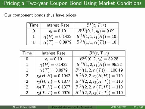
Pricing a Two-year Coupon Bond Using Market Conditions
Our component bonds thus have prices
Time Interest Rate B1(t,T , r)
0 r0 = 0.10 B(1)(0, 1, r0) = 9.09
1 r1(H) = 0.1432 B(1)(1, 1, r1(H)) = 10
1 r1(T ) = 0.0979 B(1)(1, 1, r1(T )) = 10
Time Interest Rate B2(t,T , r)
0 r0 = 0.10 B(2)(0, 2, r0) = 89.28
1 r1(H) = 0.1432 B(2)(1, 2, r1(H)) = 96.22
1 r1(T ) = 0.0979 B(2)(1, 2, r1(T )) = 100.19
2 r2(H,H) = 0.1942 B(2)(2, 2, r2(H,H)) = 110
2 r2(H,T ) = 0.1377 B(2)(2, 2, r2(H,T )) = 110
2 r2(T ,H) = 0.1377 B(2)(2, 2, r2(T ,H)) = 110
2 r2(T ,T ) = 0.0976 B(2)(2, 2, r2(T ,T )) = 110
Albert Cohen (MSU) Financial Mathematics for Actuaries I MSU Fall 2017 106 / 164
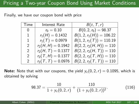
Pricing a Two-year Coupon Bond Using Market Conditions
Finally, we have our coupon bond with price
Time Interest Rate B(t,T , r)
0 r0 = 0.10 B(0, 2, r0) = 98.371 r1(H) = 0.1432 B(1, 2, r1(H)) = 106.221 r1(T ) = 0.0979 B(1, 2, r1(T )) = 110.192 r2(H,H) = 0.1942 B(2, 2, r2(H,H)) = 1102 r2(H,T ) = 0.1377 B(2, 2, r2(H,T )) = 1102 r2(T ,H) = 0.1377 B(2, 2, r2(T ,H)) = 1102 r2(T ,T ) = 0.0976 B(2, 2, r2(T ,T )) = 110
Note: Note that with our coupons, the yield yc(0, 2, r) = 0.1095, which isobtained by solving
98.37 =10
1 + yc(0, 2, r)+
110
(1 + yc(0, 2, r))2. (116)
Albert Cohen (MSU) Financial Mathematics for Actuaries I MSU Fall 2017 107 / 164
Pricing a 1-year Call Option on our 2-year Coupon Bond
Consider the previous term structure, and a European Call Option on thetwo year bond with K = 97 and expiry of 1 year.
Compute the initial Call price C0(r).
Compute the initial number of bonds to hold to replicate this option.
Albert Cohen (MSU) Financial Mathematics for Actuaries I MSU Fall 2017 108 / 164
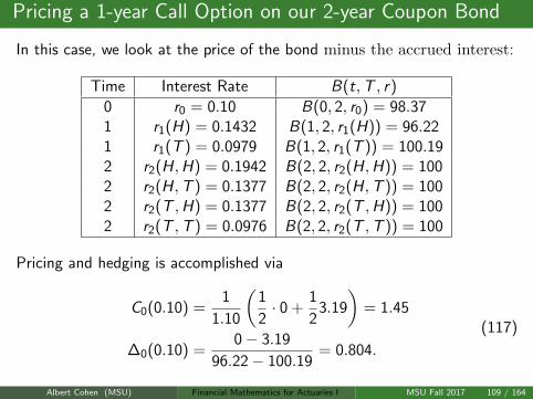
Pricing a 1-year Call Option on our 2-year Coupon Bond
In this case, we look at the price of the bond minus the accrued interest:
Time Interest Rate B(t,T , r)
0 r0 = 0.10 B(0, 2, r0) = 98.371 r1(H) = 0.1432 B(1, 2, r1(H)) = 96.221 r1(T ) = 0.0979 B(1, 2, r1(T )) = 100.192 r2(H,H) = 0.1942 B(2, 2, r2(H,H)) = 1002 r2(H,T ) = 0.1377 B(2, 2, r2(H,T )) = 1002 r2(T ,H) = 0.1377 B(2, 2, r2(T ,H)) = 1002 r2(T ,T ) = 0.0976 B(2, 2, r2(T ,T )) = 100
Pricing and hedging is accomplished via
C0(0.10) =1
1.10
(1
2· 0 +
1
23.19
)= 1.45
∆0(0.10) =0− 3.19
96.22− 100.19= 0.804.
(117)
Albert Cohen (MSU) Financial Mathematics for Actuaries I MSU Fall 2017 109 / 164

Homework
From Finan:
Problems 81.1, 81.2, 81.5, 81.6, 81.7, 81.8, 81.9.
Problems 82.1, 82.2, 82.3, 82.4, 82.5
Problems 82.6, 82.7, 82.8, 82.9, 82.10, 82.11.
Albert Cohen (MSU) Financial Mathematics for Actuaries I MSU Fall 2017 110 / 164
Lognormality
Analyzing returns, we assume:
A probability space(
Ω,F ,P).
Our asset St(ω) has an associated return over any period (t, t + u)defined as
rt,u(ω) := ln
(St+u(ω)
St(ω)
). (118)
Albert Cohen (MSU) Financial Mathematics for Actuaries I MSU Fall 2017 111 / 164
Lognormality
Partition the interval [t,T ] into n intervals of length h = T−tn , then:
The return over the entire period can be taken as the sum of thereturns over each interval:
rt,T−t(ω) = ln
(ST (ω)
St(ω)
)=
n∑k=1
rtk ,h(ω)
tk = t + kh.
(119)
We model the returns as being independent and possessing a binomialdistribution.
Employing the Central Limit Theorem, it can be shown that asn→∞, this distribution approaches normality.
Albert Cohen (MSU) Financial Mathematics for Actuaries I MSU Fall 2017 112 / 164
Binomial Tree and Discrete Dividends
Another issue encountered in elementary credit and investment theoryis the case of different compounding and deposit periods.
This also occurs in the financial setting where a dividend is not paidcontinuously, but rather at specific times.
It follows that the dividend can be modeled as delivered in the middleof a binomial period, at time τ(ω) < T .
This view is due to Schroder and can be summarized as viewing theinherent value of St(ω) as the sum of a prepaid forward PF and thepresent value of the upcoming dividend payment D:
PFt(ω) = St(ω)− De−r(τ(ω)−t)
u = erh+σ√h
d = erh−σ√h.
(120)
Now, the random process that we model as having up and downmoves is PF instead of S .
Albert Cohen (MSU) Financial Mathematics for Actuaries I MSU Fall 2017 113 / 164
Back to the Continuous Time Case
Consider the case of a security whose binomial evolution is modeled as anup or down movement at the end of each day. Over the period of oneyear, this amounts to a tree with depth 365. If the tree is not recombining,then this amounts to 2365 branches. Clearly, this is too large to evaluatereasonably, and so an alternative is sought.
Whatever the alternative, the concept of replication must hold. This isthe reasoning behind the famous Black-Scholes-Merton PDE approach.
Albert Cohen (MSU) Financial Mathematics for Actuaries I MSU Fall 2017 114 / 164
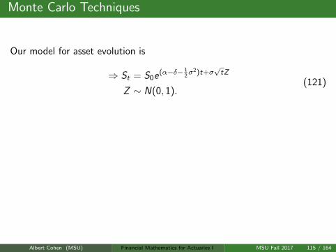
Monte Carlo Techniques
Our model for asset evolution is
⇒ St = S0e(α−δ− 12σ2)t+σ
√tZ
Z ∼ N(0, 1).(121)
Consider now the possibility of simulating the stock evolution bysimulating the random variable Z , or in fact an i.i.d. sequence
Z (i)
ni=1
.
For a European option with time expiry T , we can simulate the expirytime payoff mulitple times:
V(
S (i),T)
= G(
S (i))
= G(
S0e(α−δ− 12σ2)T+σ
√TZ (i)
). (122)
Albert Cohen (MSU) Financial Mathematics for Actuaries I MSU Fall 2017 115 / 164
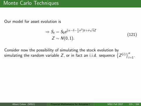
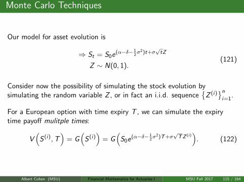
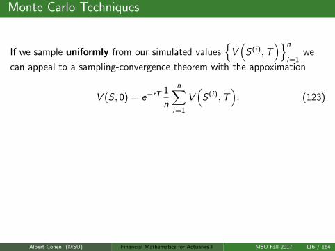
Monte Carlo Techniques
If we sample uniformly from our simulated values
V(
S (i),T)n
i=1we
can appeal to a sampling-convergence theorem with the appoximation
V (S , 0) = e−rT1
n
n∑i=1
V(
S (i),T). (123)
The challenge now is to simulate our lognormally distributed assetevolution.
One can simulate the value ST directly by one random variable Z , or amultiple of them to simulate the path of the evolution until T .
The latter method is necessary for Asian options.
Albert Cohen (MSU) Financial Mathematics for Actuaries I MSU Fall 2017 116 / 164
Monte Carlo Techniques
There are multiple ways to simulate Z . One way is to find a randomnumber U taken from a uniform distribution U[0, 1].
It follows that one can now map U → Z via inversion of the Normal cdf N:
Z = N−1(U). (124)
It can be shown that in a sample, the standard deviation of the sampleaverage σsample is related to the standard deviation of an individual drawvia
σsample =σdraw√
n. (125)
If σdraw = σ, then we can see that we must increase our sample size by22k if we wish to cut our σsample by a factor of 2k .
Albert Cohen (MSU) Financial Mathematics for Actuaries I MSU Fall 2017 117 / 164
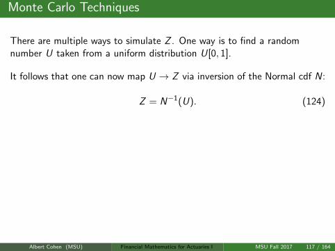
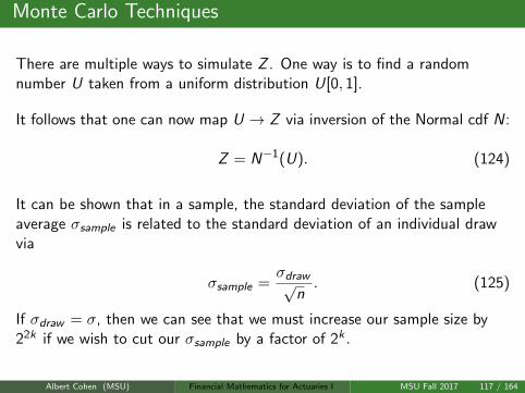
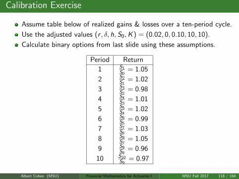
Calibration Exercise
Assume table below of realized gains & losses over a ten-period cycle.
Use the adjusted values (r , δ, h,S0,K ) = (0.02, 0, 0.10, 10, 10).
Calculate binary options from last slide using these assumptions.
Period Return
1 S1S0
= 1.05
2 S2S1
= 1.02
3 S3S2
= 0.98
4 S4S3
= 1.01
5 S5S4
= 1.02
6 S6S5
= 0.99
7 S7S6
= 1.03
8 S8S7
= 1.05
9 S9S8
= 0.96
10 S10S9
= 0.97
Albert Cohen (MSU) Financial Mathematics for Actuaries I MSU Fall 2017 118 / 164
Calibration Exercise: Linear Approximation
We would like to compute σ for the logarithm of returns ln(
SiSi−1
).
Assume the returns per period are all independent.
Q: Can we use a linear (simple) return model instead of a compoundreturn model as an approximation?
If so, then for our observed simple return rate values:
Calculate the sample variance σ2∗.
Estimate that σ ≈ σ∗√h
.
Albert Cohen (MSU) Financial Mathematics for Actuaries I MSU Fall 2017 119 / 164
Calibration Exercise: Linear Approximation
Note that if SiSi−1
= 1 + γ for γ 1, then
ln
(Si
Si−1
)≈ γ =
Si − Si−1
Si−1. (126)
Approximation: Convert our previous table, using simple interest.
Over small time periods h, define linear return values for i th period:
Xih :=Si − Si−1
Si−1. (127)
In other words, for simple rate of return Xi for period i :
Si = Si−1 · (1 + Xih). (128)
Albert Cohen (MSU) Financial Mathematics for Actuaries I MSU Fall 2017 120 / 164
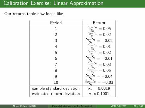
Calibration Exercise: Linear Approximation
Our returns table now looks like
Period Return
1 S1−S0S0
= 0.05
2 S2−S1S1
= 0.02
3 S3−S2S2
= −0.02
4 S4−S3S3
= 0.01
5 S5−S4S4
= 0.02
6 S6−S5S5
= −0.01
7 S7−S6S6
= 0.03
8 S8−S7S7
= 0.05
9 S9−S8S8
= −0.04
10 S10−S9S9
= −0.03
sample standard deviation σ∗ = 0.0319estimated return deviation σ ≈ 0.1001
Albert Cohen (MSU) Financial Mathematics for Actuaries I MSU Fall 2017 121 / 164
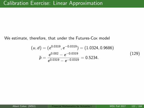
Calibration Exercise: Linear Approximation
We estimate, therefore, that under the Futures-Cox model
(u, d) = (e0.0319, e−0.0319) = (1.0324, 0.9686)
p =e0.002 − e−0.0319
e0.0319 − e−0.0319= 0.5234.
(129)
Albert Cohen (MSU) Financial Mathematics for Actuaries I MSU Fall 2017 122 / 164
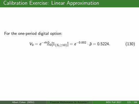
Calibration Exercise: Linear Approximation
For the one-period digital option:
V0 = e−rhE0[1S1≥10] = e−0.002 · p = 0.5224. (130)
For the two-period digital option:
V0 = e−2rhE0[1S2≥10] = e−0.004 ·[p2 + 2pq
]= 0.7698. (131)
Albert Cohen (MSU) Financial Mathematics for Actuaries I MSU Fall 2017 123 / 164
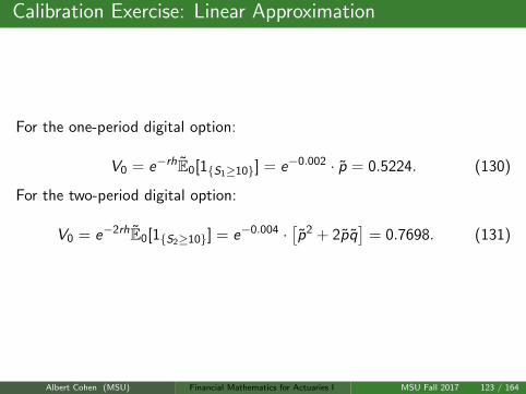
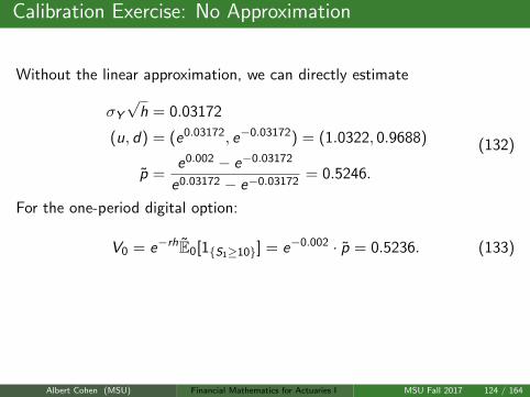
Calibration Exercise: No Approximation
Without the linear approximation, we can directly estimate
σY√
h = 0.03172
(u, d) = (e0.03172, e−0.03172) = (1.0322, 0.9688)
p =e0.002 − e−0.03172
e0.03172 − e−0.03172= 0.5246.
(132)
For the one-period digital option:
V0 = e−rhE0[1S1≥10] = e−0.002 · p = 0.5236. (133)
For the two-period digital option:
V0 = e−2rhE0[1S2≥10] = e−0.004 ·[p2 + 2pq
]= 0.7721. (134)
Albert Cohen (MSU) Financial Mathematics for Actuaries I MSU Fall 2017 124 / 164
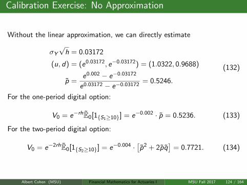
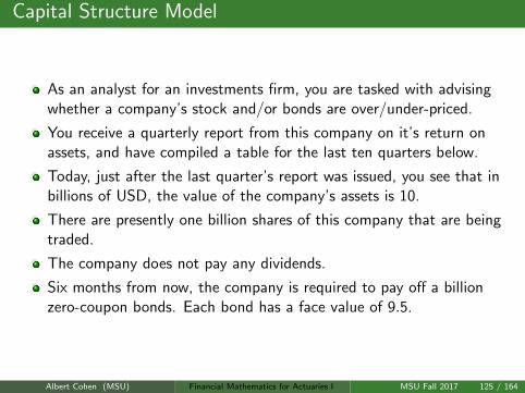
Capital Structure Model
As an analyst for an investments firm, you are tasked with advisingwhether a company’s stock and/or bonds are over/under-priced.
You receive a quarterly report from this company on it’s return onassets, and have compiled a table for the last ten quarters below.
Today, just after the last quarter’s report was issued, you see that inbillions of USD, the value of the company’s assets is 10.
There are presently one billion shares of this company that are beingtraded.
The company does not pay any dividends.
Six months from now, the company is required to pay off a billionzero-coupon bonds. Each bond has a face value of 9.5.
Albert Cohen (MSU) Financial Mathematics for Actuaries I MSU Fall 2017 125 / 164
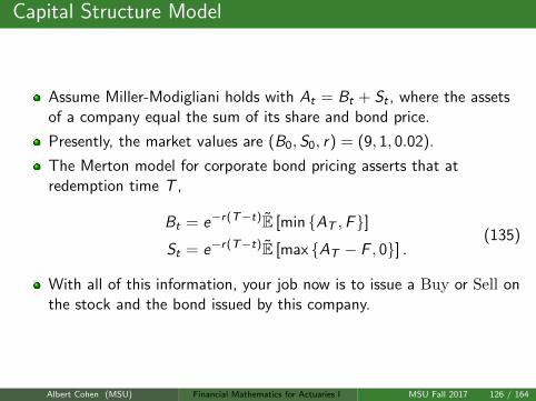
Capital Structure Model
Assume Miller-Modigliani holds with At = Bt + St , where the assetsof a company equal the sum of its share and bond price.
Presently, the market values are (B0, S0, r) = (9, 1, 0.02).
The Merton model for corporate bond pricing asserts that atredemption time T ,
Bt = e−r(T−t)E [min AT ,F]St = e−r(T−t)E [max AT − F , 0] .
(135)
With all of this information, your job now is to issue a Buy or Sell onthe stock and the bond issued by this company.
Albert Cohen (MSU) Financial Mathematics for Actuaries I MSU Fall 2017 126 / 164
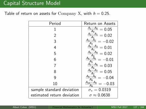
Capital Structure Model
Table of return on assets for Company X, with h = 0.25.
Period Return on Assets
1 A1−A0A0
= 0.05
2 A2−A1A1
= 0.02
3 A3−A2A2
= −0.02
4 A4−A3A3
= 0.01
5 A5−A4A4
= 0.02
6 A6−A5A5
= −0.01
7 A7−A6A6
= 0.03
8 A8−A7A7
= 0.05
9 A9−A8A8
= −0.04
10 A10−A9A9
= −0.03
sample standard deviation σ∗ = 0.0319estimated return deviation σ ≈ 0.0638
Albert Cohen (MSU) Financial Mathematics for Actuaries I MSU Fall 2017 127 / 164
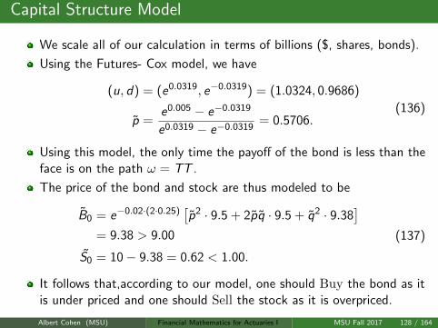
Capital Structure Model
We scale all of our calculation in terms of billions ($, shares, bonds).
Using the Futures- Cox model, we have
(u, d) = (e0.0319, e−0.0319) = (1.0324, 0.9686)
p =e0.005 − e−0.0319
e0.0319 − e−0.0319= 0.5706.
(136)
Using this model, the only time the payoff of the bond is less than theface is on the path ω = TT .
The price of the bond and stock are thus modeled to be
B0 = e−0.02·(2·0.25)[p2 · 9.5 + 2pq · 9.5 + q2 · 9.38
]= 9.38 > 9.00
S0 = 10− 9.38 = 0.62 < 1.00.
(137)
It follows that,according to our model, one should Buy the bond as itis under priced and one should Sell the stock as it is overpriced.
Albert Cohen (MSU) Financial Mathematics for Actuaries I MSU Fall 2017 128 / 164
Optimal Investment: U(x) = ln (x): Maximized over p?
In the case of a logarithmic investor, if (p, x , r) are fixed, known terms,then it follows from (43) that
u(x ; p) = ln
(1 + r)(pp
)p (1−p1−p
)1−p x
= ln (x(1 + r)) + p ln
(p
p
)+ (1− p) ln
(1− p
1− p
).
∴∂
∂p[u(x ; p)] = ln
(p
p
)− ln
(1− p
1− p
)= 0⇒ p = p.
(138)
Albert Cohen (MSU) Financial Mathematics for Actuaries I MSU Fall 2017 129 / 164
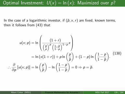
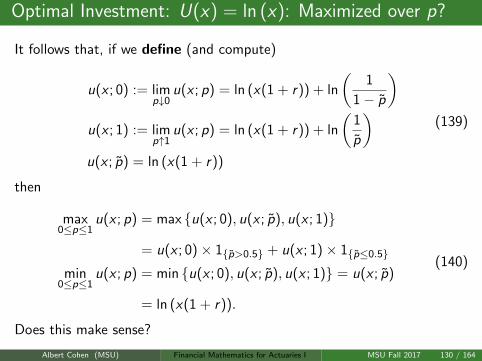
Optimal Investment: U(x) = ln (x): Maximized over p?
It follows that, if we define (and compute)
u(x ; 0) := limp↓0
u(x ; p) = ln (x(1 + r)) + ln
(1
1− p
)u(x ; 1) := lim
p↑1u(x ; p) = ln (x(1 + r)) + ln
(1
p
)u(x ; p) = ln (x(1 + r))
(139)
then
max0≤p≤1
u(x ; p) = max u(x ; 0), u(x ; p), u(x ; 1)
= u(x ; 0)× 1p>0.5 + u(x ; 1)× 1p≤0.5
min0≤p≤1
u(x ; p) = min u(x ; 0), u(x ; p), u(x ; 1) = u(x ; p)
= ln (x(1 + r)).
(140)
Does this make sense?
Albert Cohen (MSU) Financial Mathematics for Actuaries I MSU Fall 2017 130 / 164
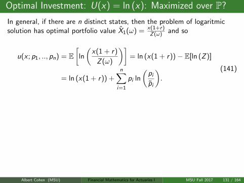
Optimal Investment: U(x) = ln (x): Maximized over P?
In general, if there are n distinct states, then the problem of logaritmicsolution has optimal portfolio value X1(ω) = x(1+r)
Z(ω) and so
u(x ; p1, .., pn) = E[
ln
(x(1 + r)
Z (ω)
)]= ln (x(1 + r))− E[ln (Z )]
= ln (x(1 + r)) +n∑
i=1
pi ln
(pi
pi
).
(141)
If we assume the pi are known, then a similar calculation as in (138) leadsto the critical physical probabilities pi = pi . This leads to a min insteadof a max solution.
Furthermore, we can see that shifting all the physical probabilities to 1 forstates i where pi < 0.5 is the maximal solution.
However, this kind of investing results in a Radon-Nikodym derivative thatis in the set 0,∞. We may need to put limits on what beliefs/physicalprobabilities we allow the investor to possess!
Albert Cohen (MSU) Financial Mathematics for Actuaries I MSU Fall 2017 131 / 164
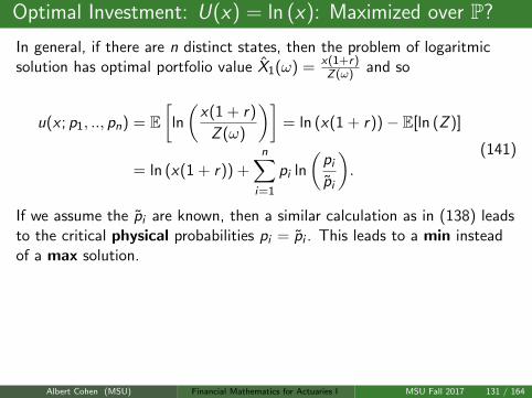
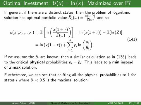
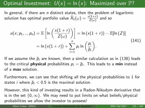
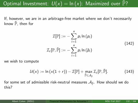
Optimal Investment: U(x) = ln (x): Maximized over P?
If, however, we are in an arbitrage-free market where we don’t necessarilyknow P, then for
I[P] := −n∑
i=1
pi ln (pi )
Ic [P, P] := −n∑
i=1
pi ln (pi )
(142)
we wish to compute
U(x) := ln (x(1 + r))− I[P] + maxP∈AP
Ic [P, P]. (143)
for some set of admissible risk-neutral measures AP. How should we dothis?
Albert Cohen (MSU) Financial Mathematics for Actuaries I MSU Fall 2017 132 / 164
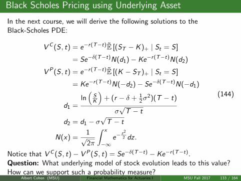
Black Scholes Pricing using Underlying Asset
In the next course, we will derive the following solutions to theBlack-Scholes PDE:
V C (S , t) = e−r(T−t)E [(ST − K )+ | St = S ]
= Se−δ(T−t)N(d1)− Ke−r(T−t)N(d2)
V P(S , t) = e−r(T−t)E [(K − ST )+ | St = S ]
= Ke−r(T−t)N(−d2)− Se−δ(T−t)N(−d1)
d1 =ln(
SK
)+ (r − δ + 1
2σ2)(T − t)
σ√
T − t
d2 = d1 − σ√
T − t
N(x) =1√2π
∫ x
−∞e−
z2
2 dz .
(144)
Notice that V C (S , t)− V P(S , t) = Se−δ(T−t) − Ke−r(T−t).Question: What underlying model of stock evolution leads to this value?How can we support such a probability measure?
Albert Cohen (MSU) Financial Mathematics for Actuaries I MSU Fall 2017 133 / 164
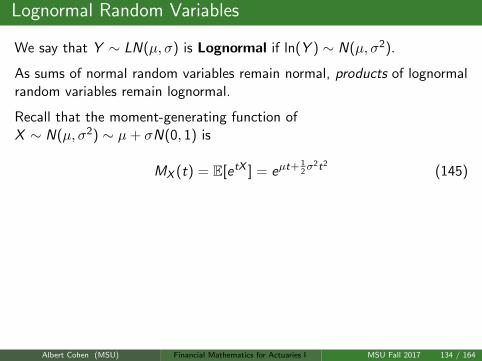
Lognormal Random Variables
We say that Y ∼ LN(µ, σ) is Lognormal if ln(Y ) ∼ N(µ, σ2).
As sums of normal random variables remain normal, products of lognormalrandom variables remain lognormal.
Recall that the moment-generating function ofX ∼ N(µ, σ2) ∼ µ+ σN(0, 1) is
MX (t) = E[etX ] = eµt+ 12σ2t2
(145)
If Y = eµ+σZ , then, it can be seen that
E[Y n] = E[enX ] = eµn+ 12σ2n2
(146)
and
fY (y) =1
σ√
2πyexp
(− (ln(y)− µ)2
2σ2
)(147)
Albert Cohen (MSU) Financial Mathematics for Actuaries I MSU Fall 2017 134 / 164
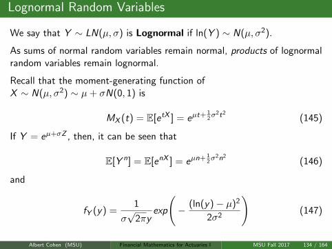
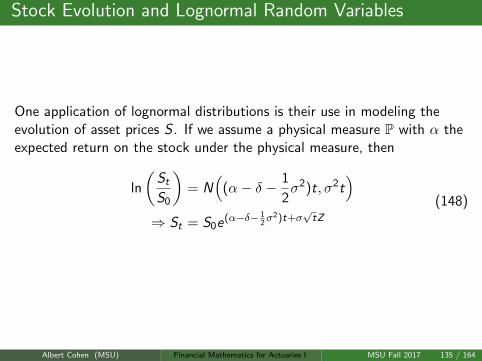
Stock Evolution and Lognormal Random Variables
One application of lognormal distributions is their use in modeling theevolution of asset prices S . If we assume a physical measure P with α theexpected return on the stock under the physical measure, then
ln
(St
S0
)= N
((α− δ − 1
2σ2)t, σ2t
)⇒ St = S0e(α−δ− 1
2σ2)t+σ
√tZ
(148)
Albert Cohen (MSU) Financial Mathematics for Actuaries I MSU Fall 2017 135 / 164
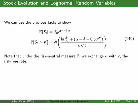
Stock Evolution and Lognormal Random Variables
We can use the previous facts to show
E[St ] = S0e(α−δ)t
P[St > K ] = N
(ln S0
K + (α− δ − 0.5σ2)t
σ√
t
).
(149)
Note that under the risk-neutral measure P, we exchange α with r , therisk-free rate:
E[St ] = S0e(r−δ)t
P[St > K ] = N(d2).(150)
Albert Cohen (MSU) Financial Mathematics for Actuaries I MSU Fall 2017 136 / 164
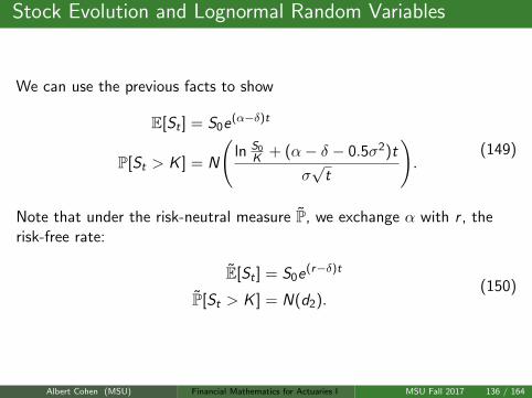
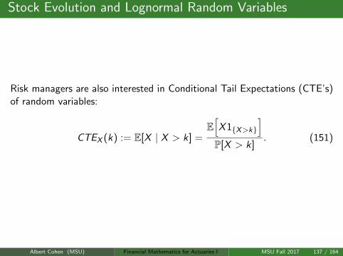
Stock Evolution and Lognormal Random Variables
Risk managers are also interested in Conditional Tail Expectations (CTE’s)of random variables:
CTEX (k) := E[X | X > k] =E[X 1X>k
]P[X > k]
. (151)
Albert Cohen (MSU) Financial Mathematics for Actuaries I MSU Fall 2017 137 / 164
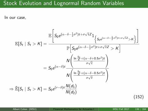
Stock Evolution and Lognormal Random Variables
In our case,
E[St | St > K ] =
E
[S0e(α−δ− 1
2σ2)t+σ
√tZ1
S0e(α−δ− 1
2σ2)t+σ
√tZ>K
]
P[S0e(α−δ− 1
2σ2)t+σ
√tZ > K
]
= S0e(α−δ)t
N
(ln
S0K
+(α−δ+0.5σ2)t
σ√t
)
N
(ln
S0K
+(α−δ−0.5σ2)t
σ√t
)
⇒ E[St | St > K ] = S0e(r−δ)t N(d1)
N(d2)(152)
Albert Cohen (MSU) Financial Mathematics for Actuaries I MSU Fall 2017 138 / 164
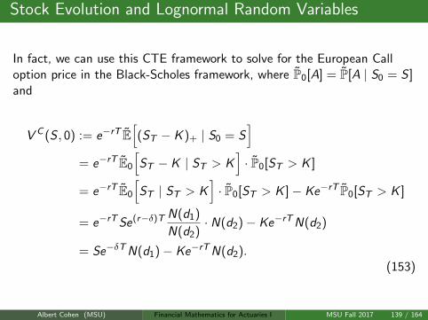
Stock Evolution and Lognormal Random Variables
In fact, we can use this CTE framework to solve for the European Calloption price in the Black-Scholes framework, where P0[A] = P[A | S0 = S ]and
V C (S , 0) := e−rT E[(ST − K )+ | S0 = S
]= e−rT E0
[ST − K | ST > K
]· P0[ST > K ]
= e−rT E0
[ST | ST > K
]· P0[ST > K ]− Ke−rT P0[ST > K ]
= e−rTSe(r−δ)T N(d1)
N(d2)· N(d2)− Ke−rTN(d2)
= Se−δTN(d1)− Ke−rTN(d2).(153)
Albert Cohen (MSU) Financial Mathematics for Actuaries I MSU Fall 2017 139 / 164
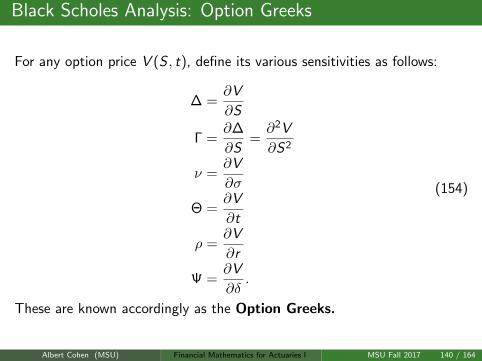
Black Scholes Analysis: Option Greeks
For any option price V (S , t), define its various sensitivities as follows:
∆ =∂V
∂S
Γ =∂∆
∂S=∂2V
∂S2
ν =∂V
∂σ
Θ =∂V
∂t
ρ =∂V
∂r
Ψ =∂V
∂δ.
(154)
These are known accordingly as the Option Greeks.
Albert Cohen (MSU) Financial Mathematics for Actuaries I MSU Fall 2017 140 / 164
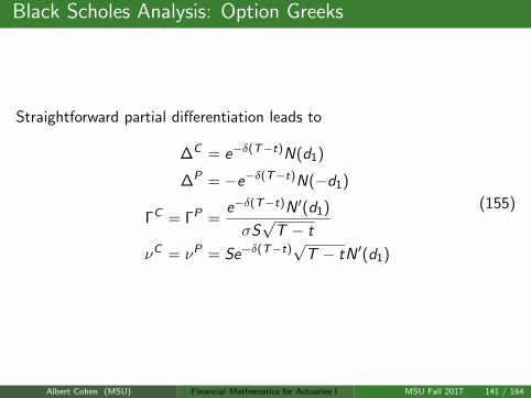
Black Scholes Analysis: Option Greeks
Straightforward partial differentiation leads to
∆C = e−δ(T−t)N(d1)
∆P = −e−δ(T−t)N(−d1)
ΓC = ΓP =e−δ(T−t)N ′(d1)
σS√
T − t
νC = νP = Se−δ(T−t)√
T − tN ′(d1)
(155)
Albert Cohen (MSU) Financial Mathematics for Actuaries I MSU Fall 2017 141 / 164
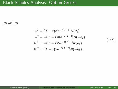
Black Scholes Analysis: Option Greeks
as well as..
ρC = (T − t)Ke−r(T−t)N(d2)
ρP = −(T − t)Ke−r(T−t)N(−d2)
ΨC = −(T − t)Se−δ(T−t)N(d1)
ΨP = (T − t)Se−δ(T−t)N(−d1).
(156)
What do the signs of the Greeks tell us?
HW: Compute Θ for puts and calls.
Albert Cohen (MSU) Financial Mathematics for Actuaries I MSU Fall 2017 142 / 164
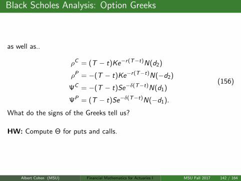
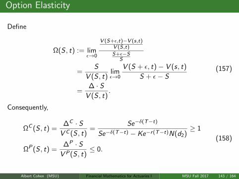
Option Elasticity
Define
Ω(S , t) := limε→0
V (S+ε,t)−V (s,t)V (S,t)
S+ε−SS
=S
V (S , t)limε→0
V (S + ε, t)− V (s, t)
S + ε− S
=∆ · S
V (S , t).
(157)
Consequently,
ΩC (S , t) =∆C · S
V C (S , t)=
Se−δ(T−t)
Se−δ(T−t) − Ke−r(T−t)N(d2)≥ 1
ΩP(S , t) =∆P · S
V P(S , t)≤ 0.
(158)
Albert Cohen (MSU) Financial Mathematics for Actuaries I MSU Fall 2017 143 / 164
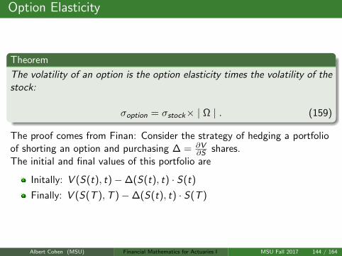
Option Elasticity
Theorem
The volatility of an option is the option elasticity times the volatility of thestock:
σoption = σstock× | Ω | . (159)
The proof comes from Finan: Consider the strategy of hedging a portfolioof shorting an option and purchasing ∆ = ∂V
∂S shares.The initial and final values of this portfolio are
Initally: V (S(t), t)−∆(S(t), t) · S(t)
Finally: V (S(T ),T )−∆(S(t), t) · S(T )
Albert Cohen (MSU) Financial Mathematics for Actuaries I MSU Fall 2017 144 / 164
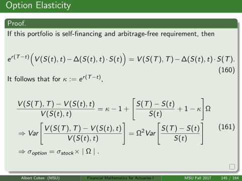
Option Elasticity
Proof.
If this portfolio is self-financing and arbitrage-free requirement, then
er(T−t)(
V (S(t), t)−∆(S(t), t) ·S(t))
= V (S(T ),T )−∆(S(t), t) ·S(T ).
(160)It follows that for κ := er(T−t),
V (S(T ),T )− V (S(t), t)
V (S(t), t)= κ− 1 +
[S(T )− S(t)
S(t)+ 1− κ
]Ω
⇒ Var
[V (S(T ),T )− V (S(t), t)
V (S(t), t)
]= Ω2Var
[S(T )− S(t)
S(t)
]⇒ σoption = σstock× | Ω | .
(161)
Albert Cohen (MSU) Financial Mathematics for Actuaries I MSU Fall 2017 145 / 164
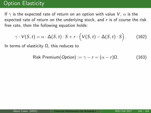
Option Elasticity
If γ is the expected rate of return on an option with value V , α is theexpected rate of return on the underlying stock, and r is of course the riskfree rate, then the following equation holds:
γ · V (S , t) = α ·∆(S , t) · S + r ·(
V (S , t)−∆(S , t) · S). (162)
In terms of elasticity Ω, this reduces to
Risk Premium(Option) := γ − r = (α− r)Ω. (163)
Furthermore, we have the Sharpe Ratio for an asset as the ratio of riskpremium to volatility:
Sharpe(Stock) =(α− r)
σ=
(α− r)Ω
σΩ= Sharpe(Call). (164)
HW Sharpe Ratio for a put? How about elasticity for a portfolio ofoptions? Now read about Calendar Spreads, Implied Volatility, andPerpetual American Options.
Albert Cohen (MSU) Financial Mathematics for Actuaries I MSU Fall 2017 146 / 164
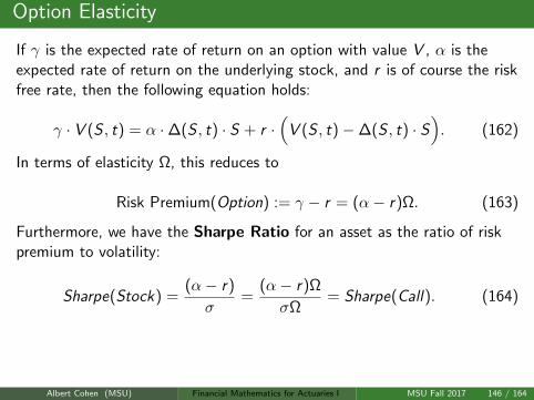
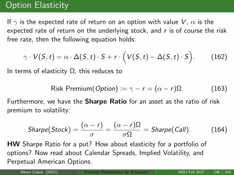
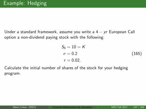
Example: Hedging
Under a standard framework, assume you write a 4− yr European Calloption a non-dividend paying stock with the following:
S0 = 10 = K
σ = 0.2
r = 0.02.
(165)
Calculate the initial number of shares of the stock for your hedgingprogram.
Albert Cohen (MSU) Financial Mathematics for Actuaries I MSU Fall 2017 147 / 164
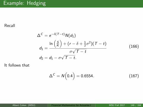
Example: Hedging
Recall
∆C = e−δ(T−t)N(d1)
d1 =ln(
SK
)+ (r − δ + 1
2σ2)(T − t)
σ√
T − t
d2 = d1 − σ√
T − t.
(166)
It follows that
∆C = N(
0.4)
= 0.6554. (167)
Albert Cohen (MSU) Financial Mathematics for Actuaries I MSU Fall 2017 148 / 164
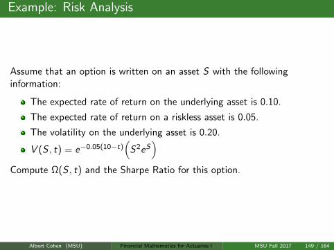
Example: Risk Analysis
Assume that an option is written on an asset S with the followinginformation:
The expected rate of return on the underlying asset is 0.10.
The expected rate of return on a riskless asset is 0.05.
The volatility on the underlying asset is 0.20.
V (S , t) = e−0.05(10−t)(
S2eS)
Compute Ω(S , t) and the Sharpe Ratio for this option.
Albert Cohen (MSU) Financial Mathematics for Actuaries I MSU Fall 2017 149 / 164
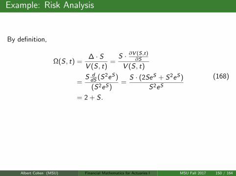
Example: Risk Analysis
By definition,
Ω(S , t) =∆ · S
V (S , t)=
S · ∂V (S,t)∂S
V (S , t)
=S d
dS (S2eS)
(S2eS)=
S · (2SeS + S2eS)
S2eS
= 2 + S .
(168)
Furthermore, since Ω = 2 + S ≥ 2, we have
Sharpe =0.10− 0.05
0.20= 0.25. (169)
Albert Cohen (MSU) Financial Mathematics for Actuaries I MSU Fall 2017 150 / 164
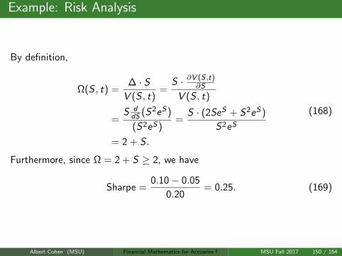
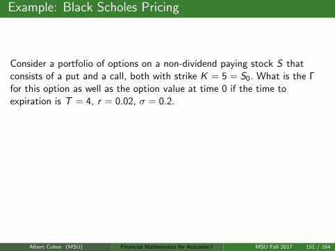
Example: Black Scholes Pricing
Consider a portfolio of options on a non-dividend paying stock S thatconsists of a put and a call, both with strike K = 5 = S0. What is the Γfor this option as well as the option value at time 0 if the time toexpiration is T = 4, r = 0.02, σ = 0.2.
In this case,
V = V C + V P
Γ =∂2
∂S2
(V C + V P
)= 2ΓC .
(170)
Albert Cohen (MSU) Financial Mathematics for Actuaries I MSU Fall 2017 151 / 164
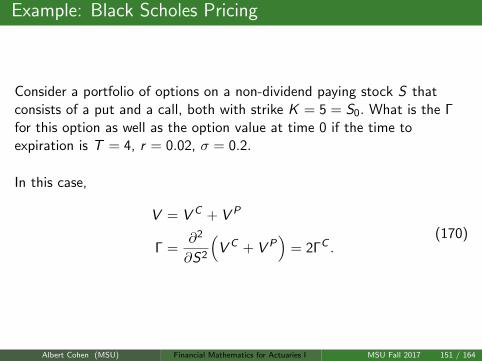
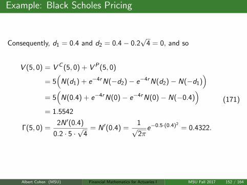
Example: Black Scholes Pricing
Consequently, d1 = 0.4 and d2 = 0.4− 0.2√
4 = 0, and so
V (5, 0) = V C (5, 0) + V P(5, 0)
= 5(
N(d1) + e−4rN(−d2)− e−4rN(d2)− N(−d1))
= 5(
N(0.4) + e−4rN(0)− e−4rN(0)− N(−0.4))
= 1.5542
Γ(5, 0) =2N ′(0.4)
0.2 · 5 ·√
4= N ′(0.4) =
1√2π
e−0.5·(0.4)2= 0.4322.
(171)
Albert Cohen (MSU) Financial Mathematics for Actuaries I MSU Fall 2017 152 / 164
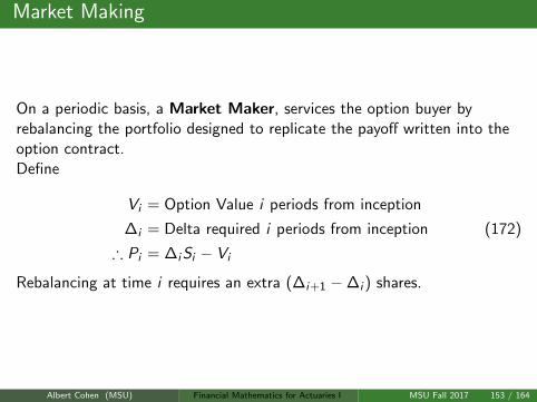
Market Making
On a periodic basis, a Market Maker, services the option buyer byrebalancing the portfolio designed to replicate the payoff written into theoption contract.Define
Vi = Option Value i periods from inception
∆i = Delta required i periods from inception
∴ Pi = ∆iSi − Vi
(172)
Rebalancing at time i requires an extra (∆i+1 −∆i ) shares.
Albert Cohen (MSU) Financial Mathematics for Actuaries I MSU Fall 2017 153 / 164
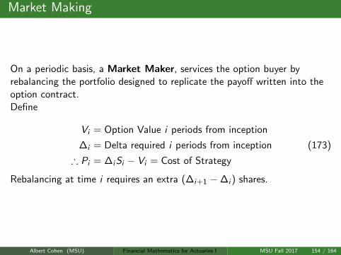
Market Making
On a periodic basis, a Market Maker, services the option buyer byrebalancing the portfolio designed to replicate the payoff written into theoption contract.Define
Vi = Option Value i periods from inception
∆i = Delta required i periods from inception
∴ Pi = ∆iSi − Vi = Cost of Strategy
(173)
Rebalancing at time i requires an extra (∆i+1 −∆i ) shares.
Albert Cohen (MSU) Financial Mathematics for Actuaries I MSU Fall 2017 154 / 164
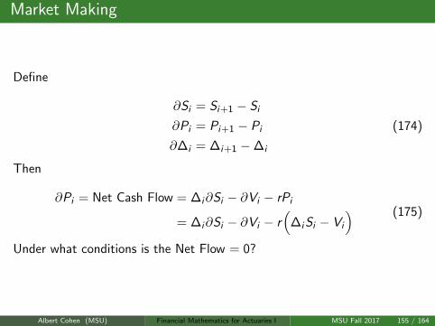
Market Making
Define
∂Si = Si+1 − Si
∂Pi = Pi+1 − Pi
∂∆i = ∆i+1 −∆i
(174)
Then
∂Pi = Net Cash Flow = ∆i∂Si − ∂Vi − rPi
= ∆i∂Si − ∂Vi − r(
∆iSi − Vi
) (175)
Under what conditions is the Net Flow = 0?
Albert Cohen (MSU) Financial Mathematics for Actuaries I MSU Fall 2017 155 / 164
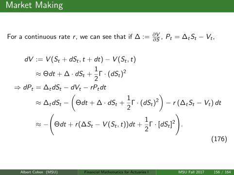
Market Making
For a continuous rate r , we can see that if ∆ := ∂V∂S , Pt = ∆tSt − Vt ,
dV := V (St + dSt , t + dt)− V (St , t)
≈ Θdt + ∆ · dSt +1
2Γ · (dSt)
2
⇒ dPt = ∆tdSt − dVt − rPtdt
≈ ∆tdSt −(
Θdt + ∆ · dSt +1
2Γ · (dSt)
2
)− r (∆tSt − Vt) dt
≈ −
(Θdt + r(∆St − V (St , t))dt +
1
2Γ · [dSt ]
2
).
(176)
Albert Cohen (MSU) Financial Mathematics for Actuaries I MSU Fall 2017 156 / 164
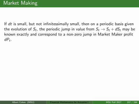
Market Making
If dt is small, but not infinitessimally small, then on a periodic basis giventhe evolution of St , the periodic jump in value from St → St + dSt may beknown exactly and correspond to a non-zero jump in Market Maker profitdPt .
If dSt · dSt = σ2S2t dt, then if we sample continuously and enforce a zero
net-flow, we retain the BSM PDE for all relevant (S , t):
∂V
∂t+ r(
S∂V
∂S− V
)+
1
2σ2S2∂
2V
∂S2= 0
V (S ,T ) = G (S) for final time payoff G (S).
(177)
Albert Cohen (MSU) Financial Mathematics for Actuaries I MSU Fall 2017 157 / 164
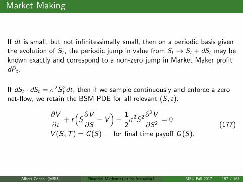
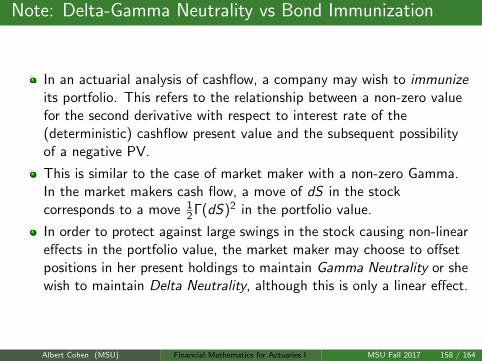
Note: Delta-Gamma Neutrality vs Bond Immunization
In an actuarial analysis of cashflow, a company may wish to immunizeits portfolio. This refers to the relationship between a non-zero valuefor the second derivative with respect to interest rate of the(deterministic) cashflow present value and the subsequent possibilityof a negative PV.
This is similar to the case of market maker with a non-zero Gamma.In the market makers cash flow, a move of dS in the stockcorresponds to a move 1
2 Γ(dS)2 in the portfolio value.
In order to protect against large swings in the stock causing non-lineareffects in the portfolio value, the market maker may choose to offsetpositions in her present holdings to maintain Gamma Neutrality or shewish to maintain Delta Neutrality, although this is only a linear effect.
Albert Cohen (MSU) Financial Mathematics for Actuaries I MSU Fall 2017 158 / 164
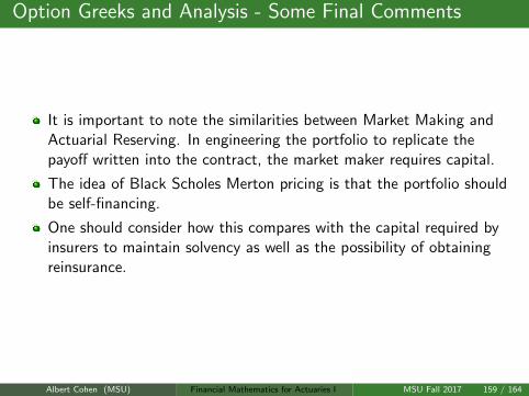
Option Greeks and Analysis - Some Final Comments
It is important to note the similarities between Market Making andActuarial Reserving. In engineering the portfolio to replicate thepayoff written into the contract, the market maker requires capital.
The idea of Black Scholes Merton pricing is that the portfolio shouldbe self-financing.
One should consider how this compares with the capital required byinsurers to maintain solvency as well as the possibility of obtainingreinsurance.
Albert Cohen (MSU) Financial Mathematics for Actuaries I MSU Fall 2017 159 / 164
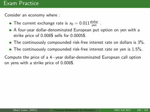
Exam Practice
Consider an economy where :
The current exchange rate is x0 = 0.011 dollaryen .
A four-year dollar-denominated European put option on yen with astrike price of 0.008$ sells for 0.0005$.
The continuously compounded risk-free interest rate on dollars is 3%.
The continuously compounded risk-free interest rate on yen is 1.5%.
Compute the price of a 4−year dollar-denominated European call optionon yens with a strike price of 0.008$.
ANSWER: By put call parity, and the Black Scholes formula, with theasset S as the exchange rate, and the foreign risk-free rate rf = δ,
V C (x0, 0) = V P(x0, 0) + x0e−rf T − Ke−rT
= 0.0005 + 0.011e−0.015·4 − 0.008e−0.03·4
= 0.003764.
(178)
Albert Cohen (MSU) Financial Mathematics for Actuaries I MSU Fall 2017 160 / 164
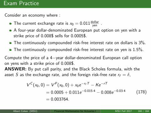
Exam Practice
Consider an economy where :
The current exchange rate is x0 = 0.011 dollaryen .
A four-year dollar-denominated European put option on yen with astrike price of 0.008$ sells for 0.0005$.
The continuously compounded risk-free interest rate on dollars is 3%.
The continuously compounded risk-free interest rate on yen is 1.5%.
Compute the price of a 4−year dollar-denominated European call optionon yens with a strike price of 0.008$.ANSWER: By put call parity, and the Black Scholes formula, with theasset S as the exchange rate, and the foreign risk-free rate rf = δ,
V C (x0, 0) = V P(x0, 0) + x0e−rf T − Ke−rT
= 0.0005 + 0.011e−0.015·4 − 0.008e−0.03·4
= 0.003764.
(178)
Albert Cohen (MSU) Financial Mathematics for Actuaries I MSU Fall 2017 160 / 164
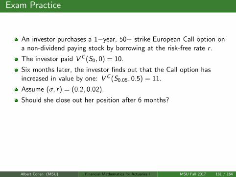
Exam Practice
An investor purchases a 1−year, 50− strike European Call option ona non-dividend paying stock by borrowing at the risk-free rate r .
The investor paid V C (S0, 0) = 10.
Six months later, the investor finds out that the Call option hasincreased in value by one: V C (S0.05, 0.5) = 11.
Assume (σ, r) = (0.2, 0.02).
Should she close out her position after 6 months?
ANSWER: Simply put, her profit if she closes out after 6 months is
11− 10e0.02 12 = 0.8995. (179)
So, yes, she should liquidate her position.
Albert Cohen (MSU) Financial Mathematics for Actuaries I MSU Fall 2017 161 / 164
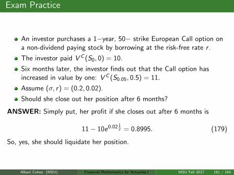

Exam Practice
Consider a 1−year at the money European Call option on anon-dividend paying stock.
You are told that ∆C = 0.65, and the economy bears a 1% rate.
Can you estimate the volatility σ?
ANSWER: By definition,
∆C = e−δTN(d1) = N( r + 1
2σ2
σ
)= N
(0.01 + 12σ
2
σ
)= 0.65
⇒0.01 + 1
2σ2
σ= 0.385
⇒ σ ∈ 0.0269, 0.7431 .
(180)
More information is needed to choose from the two roots computed above.
Albert Cohen (MSU) Financial Mathematics for Actuaries I MSU Fall 2017 162 / 164
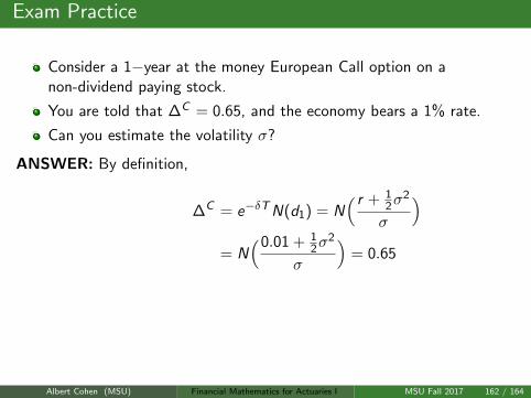
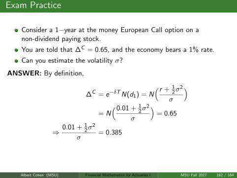
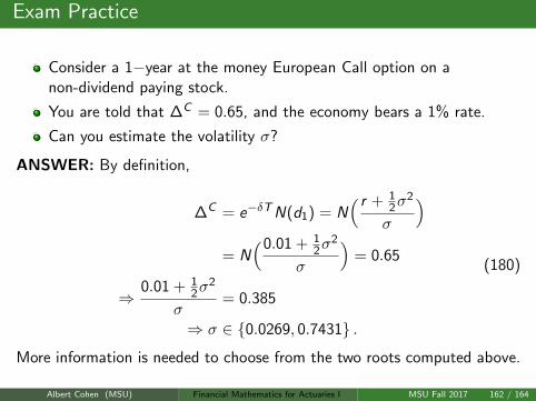

Exam Pointers
When reviewing the material for the exam, consider the followingmilestones and examples:
The definition of the Black-Scholes pricing formulae for Europeanputs and calls.
What are the Greeks? Given a specific option, could you compute theGreeks?
What is the Option Elasticity? How is it useful? How about theSharpe ratio of an option? Can you compute the Elasticity andSharpe ration of a given option?
Albert Cohen (MSU) Financial Mathematics for Actuaries I MSU Fall 2017 163 / 164
Exam Pointers
What is Delta Hedging?
If the Delta and Gamma values of an option are known, can youcalculate the change in option value given a small change in theunderlying asset value?
How does this correspond the Market Maker’s profit?
Albert Cohen (MSU) Financial Mathematics for Actuaries I MSU Fall 2017 164 / 164