Estimating a Population MeanMATH 130, Elements of Statistics I

J. Robert Buchanan

Department of Mathematics

Fall 2018

Objectives

At the end of this lesson we will be able to:I obtain a point estimate for the population mean,I state the properties of Student’s t-distribution,I determine t-values,I construct and interpret a confidence interval for a

population mean, andI find the sample size needed to estimate the population

mean within a given margin of error.

Point Estimate of the Mean

I The sample mean x is the best point estimate of thepopulation mean µ.

I Previously we constructed confidence interval estimatesfor the mean of a population assuming we knew thepopulation standard deviation σ (which is unlikely inpractice).

Lower and upper estimates: x ± zα/2 ·σ√n

I What can we do when σ is unknown?

Lower and upper estimates: x ± zα/2 ·s√n

is not correct since s, like x , is a random variable (willdepend on the sample chosen) and is not constant.

Point Estimate of the Mean

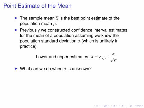
I The sample mean x is the best point estimate of thepopulation mean µ.

I Previously we constructed confidence interval estimatesfor the mean of a population assuming we knew thepopulation standard deviation σ (which is unlikely inpractice).

Lower and upper estimates: x ± zα/2 ·σ√n

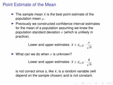
I What can we do when σ is unknown?

Lower and upper estimates: x ± zα/2 ·s√n

is not correct since s, like x , is a random variable (willdepend on the sample chosen) and is not constant.

Point Estimate of the Mean

I The sample mean x is the best point estimate of thepopulation mean µ.

I Previously we constructed confidence interval estimatesfor the mean of a population assuming we knew thepopulation standard deviation σ (which is unlikely inpractice).

Lower and upper estimates: x ± zα/2 ·σ√n

I What can we do when σ is unknown?

Lower and upper estimates: x ± zα/2 ·s√n

is not correct since s, like x , is a random variable (willdepend on the sample chosen) and is not constant.

Student’s t-Distribution

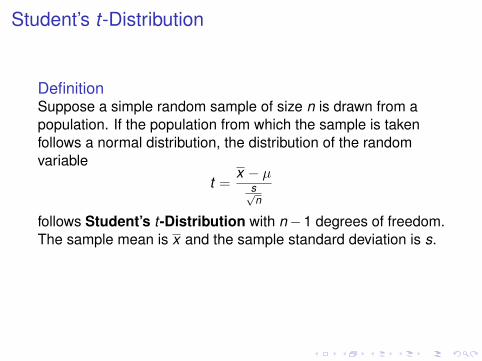
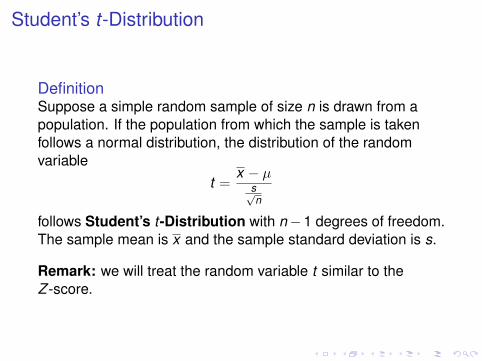
DefinitionSuppose a simple random sample of size n is drawn from apopulation. If the population from which the sample is takenfollows a normal distribution, the distribution of the randomvariable

t =x − µ

s√n

follows Student’s t-Distribution with n− 1 degrees of freedom.The sample mean is x and the sample standard deviation is s.

Remark: we will treat the random variable t similar to theZ -score.

Student’s t-Distribution

DefinitionSuppose a simple random sample of size n is drawn from apopulation. If the population from which the sample is takenfollows a normal distribution, the distribution of the randomvariable

t =x − µ

s√n

follows Student’s t-Distribution with n− 1 degrees of freedom.The sample mean is x and the sample standard deviation is s.

Remark: we will treat the random variable t similar to theZ -score.

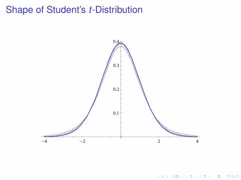
Shape of Student’s t-Distribution

-4 -2 2 4

0.1

0.2

0.3

0.4

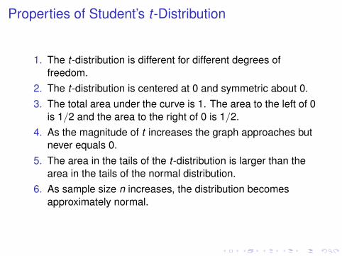
Properties of Student’s t-Distribution

1. The t-distribution is different for different degrees offreedom.

2. The t-distribution is centered at 0 and symmetric about 0.3. The total area under the curve is 1. The area to the left of 0

is 1/2 and the area to the right of 0 is 1/2.4. As the magnitude of t increases the graph approaches but

never equals 0.5. The area in the tails of the t-distribution is larger than the

area in the tails of the normal distribution.6. As sample size n increases, the distribution becomes

approximately normal.

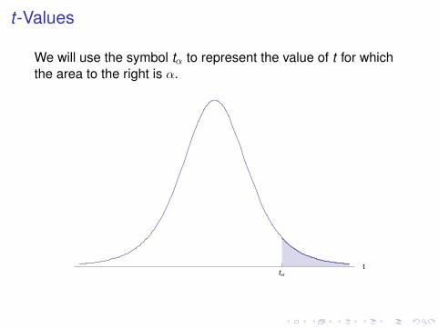
t-Values

We will use the symbol tα to represent the value of t for whichthe area to the right is α.

tΑ

t

Determining t-Values

We can look up tα in Table VI.

To use this table we must know:I the degrees of freedom df = n − 1,I the area in the right tail of the distribution.

Confidence Intervals

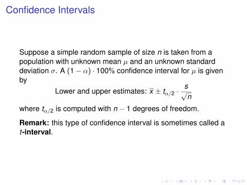
Suppose a simple random sample of size n is taken from apopulation with unknown mean µ and an unknown standarddeviation σ. A (1− α) · 100% confidence interval for µ is givenby

Lower and upper estimates: x ± tα/2 ·s√n

where tα/2 is computed with n − 1 degrees of freedom.

Remark: this type of confidence interval is sometimes called at-interval.

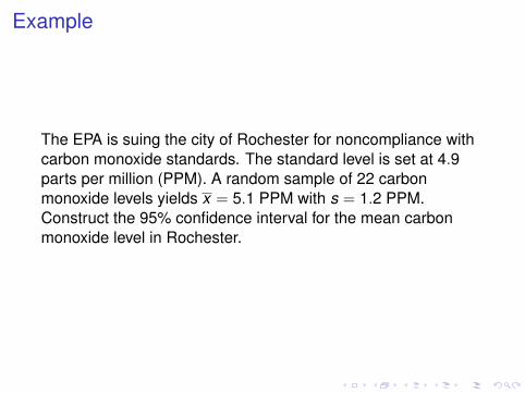
Example

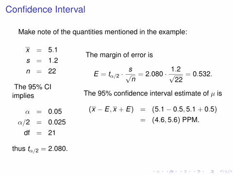
The EPA is suing the city of Rochester for noncompliance withcarbon monoxide standards. The standard level is set at 4.9parts per million (PPM). A random sample of 22 carbonmonoxide levels yields x = 5.1 PPM with s = 1.2 PPM.Construct the 95% confidence interval for the mean carbonmonoxide level in Rochester.

Confidence Interval

Make note of the quantities mentioned in the example:

x = 5.1s = 1.2n = 22

The 95% CIimplies

α = 0.05α/2 = 0.025

df = 21

thus tα/2 = 2.080.

The margin of error is

E = tα/2 ·s√n= 2.080 · 1.2√

22= 0.532.

The 95% confidence interval estimate of µ is

(x − E , x + E) = (5.1− 0.5,5.1 + 0.5)= (4.6,5.6) PPM.

Confidence Interval

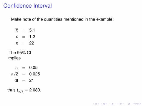
Make note of the quantities mentioned in the example:

x = 5.1s = 1.2n = 22

The 95% CIimplies

α = 0.05α/2 = 0.025

df = 21

thus tα/2 = 2.080.

The margin of error is

E = tα/2 ·s√n= 2.080 · 1.2√

22= 0.532.

The 95% confidence interval estimate of µ is

(x − E , x + E) = (5.1− 0.5,5.1 + 0.5)= (4.6,5.6) PPM.

Confidence Interval

Make note of the quantities mentioned in the example:

x = 5.1s = 1.2n = 22

The 95% CIimplies

α = 0.05α/2 = 0.025

df = 21

thus tα/2 = 2.080.

The margin of error is

E = tα/2 ·s√n= 2.080 · 1.2√

22= 0.532.

The 95% confidence interval estimate of µ is

(x − E , x + E) = (5.1− 0.5,5.1 + 0.5)= (4.6,5.6) PPM.

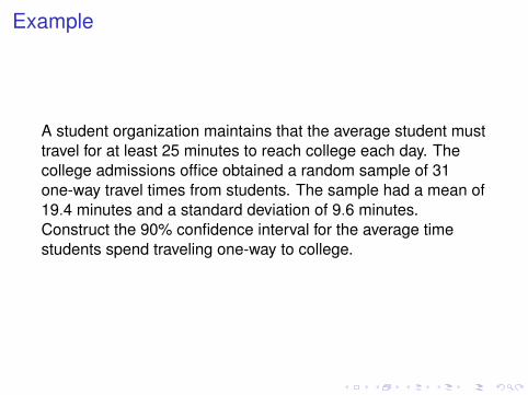
Example

A student organization maintains that the average student musttravel for at least 25 minutes to reach college each day. Thecollege admissions office obtained a random sample of 31one-way travel times from students. The sample had a mean of19.4 minutes and a standard deviation of 9.6 minutes.Construct the 90% confidence interval for the average timestudents spend traveling one-way to college.

Confidence Interval

Make note of the quantities mentioned in the example:

x = 19.4s = 9.6n = 31

The 90% CIimplies

α = 0.10α/2 = 0.05

df = 30

thus tα/2 = 1.697.

The margin of error is

E = tα/2 ·s√n= 1.697 · 9.6√

31= 2.926.

The 90% confidence interval estimate of µ is

(x − E , x + E) = (19.4− 2.9,19.4 + 2.9)= (16.5,22.3) minutes.

Confidence Interval

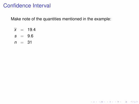
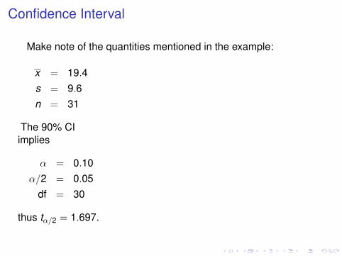
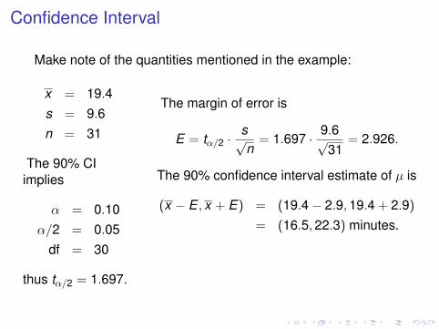
Make note of the quantities mentioned in the example:

x = 19.4s = 9.6n = 31

The 90% CIimplies

α = 0.10α/2 = 0.05

df = 30

thus tα/2 = 1.697.

The margin of error is

E = tα/2 ·s√n= 1.697 · 9.6√

31= 2.926.

The 90% confidence interval estimate of µ is

(x − E , x + E) = (19.4− 2.9,19.4 + 2.9)= (16.5,22.3) minutes.

Confidence Interval

Make note of the quantities mentioned in the example:

x = 19.4s = 9.6n = 31

The 90% CIimplies

α = 0.10α/2 = 0.05

df = 30

thus tα/2 = 1.697.

The margin of error is

E = tα/2 ·s√n= 1.697 · 9.6√

31= 2.926.

The 90% confidence interval estimate of µ is

(x − E , x + E) = (19.4− 2.9,19.4 + 2.9)= (16.5,22.3) minutes.

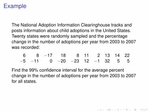
Example

The National Adoption Information Clearinghouse tracks andposts information about child adoptions in the United States.Twenty states were randomly sampled and the percentagechange in the number of adoptions per year from 2003 to 2007was recorded:

6 8 −17 18 8 11 2 13 14 22−5 −11 0 −20 −23 12 −1 32 5 5

Find the 99% confidence interval for the average percentchange in the number of adoptions per year from 2003 to 2007for all states.

Hint: x = 4.0 and s = 14.0.

Example

The National Adoption Information Clearinghouse tracks andposts information about child adoptions in the United States.Twenty states were randomly sampled and the percentagechange in the number of adoptions per year from 2003 to 2007was recorded:

6 8 −17 18 8 11 2 13 14 22−5 −11 0 −20 −23 12 −1 32 5 5

Find the 99% confidence interval for the average percentchange in the number of adoptions per year from 2003 to 2007for all states.

Hint: x = 4.0 and s = 14.0.

Confidence Interval

Make note of the quantities mentioned in the example:

x = 4.0s = 14.0n = 20

The 99% CIimplies

α = 0.01α/2 = 0.005

df = 19

thus tα/2 = 2.861.

The margin of error is

E = tα/2 ·s√n= 2.861 · 14.0√

20= 8.956.

The 99% confidence interval estimate of µ is

(x − E , x + E) = (4.0− 9.0,4.0 + 9.0)= (−5.0,13.0) percent.

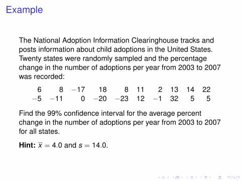
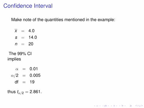
Confidence Interval

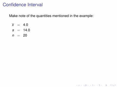
Make note of the quantities mentioned in the example:

x = 4.0s = 14.0n = 20

The 99% CIimplies

α = 0.01α/2 = 0.005

df = 19

thus tα/2 = 2.861.

The margin of error is

E = tα/2 ·s√n= 2.861 · 14.0√

20= 8.956.

The 99% confidence interval estimate of µ is

(x − E , x + E) = (4.0− 9.0,4.0 + 9.0)= (−5.0,13.0) percent.

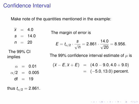
Confidence Interval

Make note of the quantities mentioned in the example:

x = 4.0s = 14.0n = 20

The 99% CIimplies

α = 0.01α/2 = 0.005

df = 19

thus tα/2 = 2.861.

The margin of error is

E = tα/2 ·s√n= 2.861 · 14.0√

20= 8.956.

The 99% confidence interval estimate of µ is

(x − E , x + E) = (4.0− 9.0,4.0 + 9.0)= (−5.0,13.0) percent.

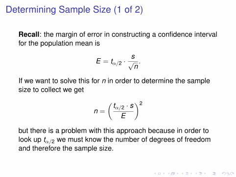
Determining Sample Size (1 of 2)

Recall: the margin of error in constructing a confidence intervalfor the population mean is

E = tα/2 ·s√n.

If we want to solve this for n in order to determine the samplesize to collect we get

n =

(tα/2 · s

E

)2

but there is a problem with this approach because in order tolook up tα/2 we must know the number of degrees of freedomand therefore the sample size.

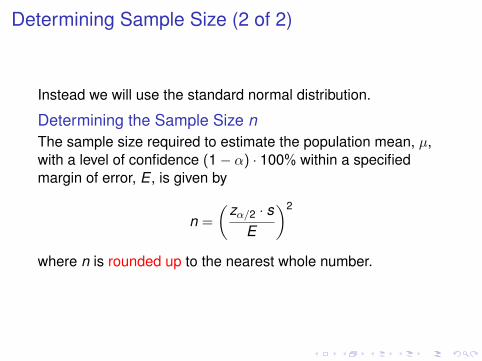
Determining Sample Size (2 of 2)

Instead we will use the standard normal distribution.

Determining the Sample Size nThe sample size required to estimate the population mean, µ,with a level of confidence (1− α) · 100% within a specifiedmargin of error, E , is given by

n =

(zα/2 · s

E

)2

where n is rounded up to the nearest whole number.

Example

Suppose a previous study has shown the sample standarddeviation of a particular model of automobile to be 3.12 mpg.

How large a sample is necessary to estimate the mean milesper gallon to within 0.25 mpg with 95% confidence?

Reading carefully above we have s = 3.12, E = 0.25, andα = 0.05 which implies zα/2 = 1.96.

n =

(zα/2 · s

E

)2

=

(1.96 · 3.12

0.25

)2

= 598.33 ≈ 599

Example

Suppose a previous study has shown the sample standarddeviation of a particular model of automobile to be 3.12 mpg.

How large a sample is necessary to estimate the mean milesper gallon to within 0.25 mpg with 95% confidence?

Reading carefully above we have s = 3.12, E = 0.25, andα = 0.05 which implies zα/2 = 1.96.

n =

(zα/2 · s

E

)2

=

(1.96 · 3.12

0.25

)2

= 598.33 ≈ 599

Example

Suppose a previous study has shown the sample standarddeviation of a particular model of automobile to be 3.12 mpg.

How large a sample is necessary to estimate the mean milesper gallon to within 0.25 mpg with 95% confidence?

Reading carefully above we have s = 3.12, E = 0.25, andα = 0.05 which implies zα/2 = 1.96.

n =

(zα/2 · s

E

)2

=

(1.96 · 3.12

0.25

)2

= 598.33 ≈ 599