Materials Design and Prediction Using Computational Science · band calculation in order to obtain the optical band gap. The optical band gap was estimated using the energy difference

1SUMITOMO KAGAKU 2015

This paper is translated from R&D Repor t, “SUMITOMO KAGAKU”, vol. 2015.

Initially, we applied it to the design of agrochemicals.

However, along with technology innovation and the sig-

nificant evolution of computers, it has developed into

materials design, as intended for larger, more complex

structures (hereinafter referred to as “computational

materials science”, which corresponds to “Simulation

and Prediction” in Fig. 1), and it now occupies an impor-

tant position in our materials development.

The situation surrounding computational science is

now undergoing significant change. Particularly, since

2000 many computational science software programs

have become compatible with parallel computation due

to the dissemination of general-purpose parallel comput-

ers. This trend has accelerated the speed-up of scientific

computation and the expansion of its scale in industry.

Parallel to such a trend, the industrial use of domestic

large-scale computers has been promoted, thus acceler-

ating the industrial use of the “Earth Simulator” of the

Japan Agency for Marine-Earth Science and Technolo-

gy, as well as “TSUBAME” of the Tokyo Institute of

Technology. Moreover, September 2012 brought the full

operation of a supercomputer called “K” (hereinafter

referred to as the K computer) developed by the Nation-

al Research and Development Agency RIKEN, thus

allowing industrial users to take advantage of its tremen-

dously improved computational capability.2) We have

also used the K computer since its initial operation in

order to establish the fundamental techniques for the

future of large-scale calculation of material structures

Materials Design and PredictionUsing Computational Science

Sumitomo Chemical Co., Ltd.

Advanced Materials Research Laboratory

Masaya ISHIDA

Yasuyuki KURITA

Akiko NAKAZONO

Recent progress in simulation and computer technology has helped the growth of computational materials science.Computer aided design of materials with high functionality based on theories of materials science has become animportant and essential part of research and development in our company. Here, we introduce our work on thecomputational analysis of inorganic fluorescent and organic semiconductor materials. Also, we show how recentprogress in this field can influence the directions of our research in the future.

Introduction

Computational science has, in recent years, been

referred to as the “third science” in addition to experi-

mental and theoretical approaches. It consists of four

areas, as shown in Fig. 1.1)

Sumitomo Chemical has positioned computational sci-

ence as one of the useful methods for our various

research and development. It has been used to present

the direction of research and development, such as in

proposing indices for efficient screening of chemical

compounds and proposing structures of high-perfor-

mance materials.

As described in later sections, we at Sumitomo Chem-

ical have a long history and experience in molecular

design to predict molecular structures and functions.

Fig. 1 Schematic overview of four functions of computational science pictured by the author based on reference 1

Simulationand

Prediction

Observationand

Modeling

Application toSocial Science Data Science

ComputationalScience


Materials Design and Prediction Using Computational Science

and electronic states. In this paper we will introduce our

computational approaches from molecular design to

materials design, presenting practical examples, and will

discuss how computational materials science is applied

in industrial materials development and the future per-

spectives.

This paper consists of as follows: The next section will

review the history of computational science in Sumito-

mo Chemical as well as some practical examples of com-

putational materials science in our Advanced Materials

Research Laboratory in Tsukuba. Lastly, we will review

the recent trend in computational materials science and

present our goals in computational science in our com-

pany based on the above reviews and examples.

Our Approach to Computational Science

1. History of Computational Science in Sumitomo

Chemical

The origin of computational science in our company

is research in the structure-activity relationship of agro-

chemicals, which began at the laborator y in the

Takarazuka district during the 1970s. The Hansch-Fujita

method3)— which is used for multiple regression analy-

ses between agrochemical activities (insecticidal, fungi-

cidal, herbicidal activities) and the hydrophobic, electri-

cal and steric parameters of a substituent group that

substitutes for a hydrogen atom on the parent chemical

structure of an agrochemical — was applied to the devel-

opment of agrochemicals such as the herbicide named

Sumiherb®.4) When there are multiple substitution sites,

it is difficult to find the combination of substituents that

will optimize the agrochemical activities. In order to

solve this issue, Takayama and Yoshida et al. have

developed a computer program named PREHAC, which

puts parameters stored in the substituent-parameter

database into the correlation equation obtained from a

structure-activity relationship analysis, predicts the activ-

ities of various substitution combinations, and outputs

the activities in descending order.5) It can be said that

the PREHAC is a pioneering software program for mate-

rials informatics which is now attracting global attention.

Subsequently, during the 1980s Sumitomo Chemical

jointly developed the computer chemistr y system

named ACACS6) together with NEC Corporation by

expanding PREHAC and other similar programs. The

ACACS system was then applied not only to structure-

activity correlation analysis of agrochemicals7) – 11), but

also to characteristics analysis of synthetic dyes and the

like. In 1990, Yoshida, one of the ACACS developers,

moved to the Tsukuba Laboratory with Zempo (current-

ly working as a professor at Hosei University) et al., and

further expanded the scope of computer chemistry to

encompass materials design and device design, and con-

sequently it evolved to computational materials sci-

ence.12)

2. Examples of Our Approach to Computational

Materials Science

The process of industrial materials development con-

sists not only of exploring molecules and materials hav-

ing outstanding characteristics and functionalities as raw

materials, but also of a series of efforts to optimize vari-

ous parameters of the material so that it will demon-

strate the desired characteristics and functions in sys-

tems such as electric devices and launch it to the market

as a final product. This process is closely related to the

hierarchical structure of materials. For example, in elec-

tronics-related materials, atoms and molecules aggre-

gate and form a more complex higher-order structure,

then the aggregates are incorporated into devices and

finally the device properties are demonstrated.

One of the required roles of computational materials

science is to improve the efficiency of research and

development through the following activities: revealing

the nature of phenomena derived from various forms of

matter during such a successive development stages;

based on understanding of the nature, inspiring new

ideas through the prediction of characteristics and func-

tions that each material and its aggregate structure may

demonstrate; and contributing to the creation of new or

highly functional materials and innovative processes.

This section will introduce four practical examples of

our approach to computational materials science. First,

we will introduce the computational material search

using optical band gap prediction for inorganic phospho-

rs, followed by the results of investigation into the

methodologies regarding the conduction characteristics

and optical properties of organic semiconductor materi-

als through the use of TSUBAME of the Tokyo Institute

of Technology and the K computer. Lastly, we will intro-

duce the result of investigation into the solubility pre-

diction of chemical compounds, such prediction being

crucial for the coating process.

(1) Computational Material Search Using the Optical

Band Gap Prediction of Inorganic Phosphors

Inorganic phosphors are used for plasma displays and



scintillation materials, as well as in lighting such as flu-

orescent lights. The luminescent colors of red, green

and blue can be obtained from inorganic phosphors,

depending on the kinds of doped rare-earth elements

and their valences. The inorganic phosphors introduced

here are Eu2+ doped silicate materials, which show blue

luminescent color due to vacuum UV excitation (wave-

lengths of 147nm and 172nm).13) It is generally consid-

ered that during the light absorption/emission process

of inorganic phosphors, once a host crystal of an oxide

or the like has absorbed vacuum UV rays, its energy is

transferred to a doped rare-earth element, thereby caus-

ing the element to illuminate.14) Therefore, from the per-

spective of material search, the question of how to find

host crystals having the optical band gap, which corre-

sponds to two types of the excitation wavelength of vac-

uum UV rays, is crucially important.

The optical band gap of a host crystal is calculated

using the first-principles band calculation method.

Although the calculated optical band gap is often small-

er than the experimental value due to the approxima-

tion contained in the original theory, it is well known

that its qualitative tendency derived from the difference

in materials is often reproduced.15) In our search for sil-

icate host crystals suitable for the excitation wave-

lengths of 147nm and 172nm, we calculated the optical

band gaps of various types of silicates using the band

calculation.16)

In this study we extracted approximately 30 crystal

structure data for silicates having different compositions

from the inorganic crystal structure database, then we

carried out a structure-optimization calculation via the

band calculation in order to obtain the optical band gap.

The optical band gap was estimated using the energy

difference (Ediff) between the valence band edge of the

density-of-state and the first peak of the d band. Fig. 2

shows the results. Because it is known that CMS

(CaMgSi2O6) (shown at the far-left of Fig. 2) has 147nm

absorption , all the calculated optical band gaps are shift-

ed by adding the energy difference between the experi-

mental value 8.4 eV(147nm) and the calculated value of

CMS.

The aluminate host crystal BAM (BaMgAl10O17)

known as a commercialized blue color inorganic phos-

phor has 172nm absorption, and the calculated value of

the optical band gap of BAM corresponds well to its

excitation energy (7.2eV). Based on this calculation

result, we predict that BaCa2MgSi2O8 and BaCa2Si3O9,

which are present in the vicinity of BAM, should be

promising candidate silicates corresponding to 172nm

excitation. In fact, BaCa2MgSi2O8 was developed as an

inorganic phosphor corresponding to 172nm excitation.

The calculation result is consistent with the experiment.

We use the term “computational material screening”

for the method of reducing the number of candidates

by calculating characteristics of chemical compounds

Fig. 2 The host excitation energies of various non-doped silicate hosts, estimated by using the energy difference

(Ediff) between the VB top and the first maximum intense d band calculated using the VASP code 17). The scissors operator of 1.4 eV for all unoccupied bands is uniformly applied. The dashed line at 7 eV indicates

the uncorrected value of Ediff for CMS.© IOP Publishing. Reproduced by permission of IOP Publishing. All rights reserved.

0

1

2

3

4

5

6

7

8

9

CM

SC

aA

l2(S

i,A

l)O

6

Ca

2A

l2S

iO7

CaZ

nS

i3O

8

Ba

Al2

Si2

O8_

2(C

a,B

a3)

Si2

B2O

8

SrS

iO3

CaS

iO3

CaS

i2B

2O8

BaS

i4O

9

BaS

i2B

2O8

Sr2

Al2

SiO

7

Ca

3Mg

Si2

O8

(Ca,

Mg

2)S

i2O

7

Ba

Al2

Si2

O8

BaC

a2M

gS

i2O

8

BA

MB

aCa

2S

i3O

9

BaS

i2O

5

BaZ

nS

i3O

8

BaS

iO3

Ca5

SiP

2O1

2

(Ca

2,M

g)S

i2O

7

Ba4

Si6

O16

Ba

3Mg

Si2

O8

Ca

3S

i2O

7

BaM

gS

iO4

BaS

nS

i3O

9

BaC

aSiO

4

CaS

rSiO

4

Ca

2(M

g,A

l)(S

i,A

l)2O

7

CaM

g3S

i3O

10

Ca

2S

iO4

Sr3

SiO

5

Ca

3S

iO5

Ca

3S

nS

i2O

9

Mg

2S

iO4

Ed

iff (

eV)



describes our investigation of the hole-injection property

and hole conductivity.

( i) Hole-Injectability from Electrode to Organic Semi-

conductor

One of the factors that affect the injection of holes

from an electrode to an organic semiconductor is the

difference between the Fermi energy of the electrode

material and the valence band top energy of the organic

semiconductor. The smaller this energy difference is,

the more often hole injection will occur, thus causing

the electric resistance to become smaller. This is ideal

from the perspective of economical power consumption.

In an experiment the valence band top energy of the

organic semiconductor is evaluated as a negative value

of the ionization potential, which is measured using pho-

toelectron spectroscopy. In a theoretical calculation it is

often evaluated by calculating the HOMO (Highest

Occupied Molecular Orbital) levels of single molecules.

However, because an organic semiconductor is an

aggregate composed of numerous organic semiconduc-

tor molecules, it is affected by the intermolecular inter-

actions such as π - π interaction, and consequently the

tendency of the measured ionization potential may not

be explained merely by the calculated values of the

HOMO levels of single molecules. An example is shown

below.18)

We examined the ionization potentials of low-molecu-

lar organic semiconductors as a foundation for predict-

and materials using theoretical methods. Currently,

although there is an issue of calculation accuracy, it can

be expected that if computational material screening is

applied to an even broader search for chemical com-

pounds and materials, it will improve the efficiency of

material search. For more detailed analysis of the mech-

anism of photo-excitation and luminescence, please see

the reference.16)

(2) Design of Organic Semiconductor Materials

Organic EL (electroluminescence) displays, transis-

tors and solar cells can be manufactured through rela-

tively inexpensive process methods such as inkjet and

printing methods. They have garnered attention as next-

generation devices having favorable characteristics such

as light weight, thinness and flexibility. Organic semi-

conductors are the key materials in the above devices.

The important factors when an organic semiconduc-

tor demonstrates its functions are carrier (electrons or

holes) injection from the electrodes and carrier conduc-

tion within the organic semiconductor. Additionally, light

emission (which occurs due to the recombination of

electrons and holes) is important for organic EL dis-

plays, and the electron-hole pair generation from the

excited states (which occurs due to light absorption) is

crucial for organic solar cells. Furthermore, it is known

that the characteristics (such as crystallinity) of the

aggregated structure of organic-semiconductor mole-

cules greatly affect the above process. The following

Fig. 3 Molecular structures of organic semiconductors for ionization potential calculations

Acene-type Amine-type

N N

NN

NN



sity occurs in multiple molecules when ionized, as seen

in the example of pentacenes in Fig. 5.

(ii) Hole Conductivity in Organic Semiconductors

Of the three devices listed in a previous section, the

improvement of carrier mobility in an organic semicon-

ductor is important in order to improve the performance

of organic transistors in particular. When the voltage

between the electrodes is constant, electric current can

be increased by increasing the carrier mobility. The

application of organic transistors to adjustment of the

brightness of pixels of flexible organic EL displays has

been examined. However, because a certain amount of

electric current is required at low voltage, the improve-

ment of carrier mobility is necessary from the stand-

point of economical power consumption.

ing the aforementioned hole-injectability. Regarding sin-

gle molecules, which constitute each of the low-molecu-

lar organic semiconductors shown in Fig. 3 and were

isolated from measured single crystal structures, the

left graph in Fig. 4 depicts the relationship between the

measured ionization potential and the calculated ioniza-

tion potential as a difference between the energy of the

neutral state and that of the cation radial state using

the density functional method (B3LYP/6-31G* level)

through the Gaussian09 program.20) The acene-type

low-molecular compounds (●) and amine-type low-

molecular compounds (○) are described using different

correlation lines. However, when calculating the ioniza-

tion potential including the first-nearest-neighbor mol-

ecules in the measured single crystal structure21), the

correlation lines of the acene-based and amine-based

low-molecular compounds become closer to one anoth-

er. Furthermore, if this calculation includes the second-

nearest-neighbor molecules, the correlation lines of

both molecules will nearly overlap. When this occurs,

the correlation between the total experimental value

and the total calculated value of the acene-based and

amine-based molecules are 0.73, 0.89 and 0.98 for the

isolated molecule model, first-nearest-neighbor model

and second-nearest-neighbor model, respectively.

The above results indicate that in order to compre-

hensively understand the tendencies of the ionization

potentials of various organic semiconductors, the calcu-

lation for single molecules is insufficient. It is therefore

necessary to use a calculation model for a molecular

aggregate that includes at least the first- and the sec-

ond-nearest-neighbor molecules. It can be surmised that

this is due to the fact that the delocalization of spin den-

Fig. 4 Experimental and calculated ionization potentials

4

5

6

7

8

4 5 6 7 84

5

6

7

8

4 5 6 7 84

5

6

7

8

4 5 6 7 8

Exp

erim

enta

lIo

niz

atio

n P

oten

tial

(eV

)

Calculated Ionization Potential (eV)

Isolated Molecules Isolated and First-Nearest-Neighbor

Molecules

Isolated, First- and Second-Nearest-Neighbor

Molecules

Fig. 5 Spin density calculated for isolated, first- and second-nearest-neighbor pentacenes



The theories and methods to calculate the carrier con-

ductivity in organic semiconductors include the Marcus

theory22), band theory23), non-equilibrium Green’s func-

tion method24) and time-dependent Schrödinger equa-

tion.25) Below are shown examples of our application of

the intra-chain current calculated through the non-equi-

librium Green’s function method as an index for the

electric conductivity in polymer chains, and the reso-

nance integral between the HOMOs of polymer chains

as an index for the electric conductivity between the

polymer chains.26)

The application of the non-equilibrium Green’s func-

tion method to molecules was initiated by Datta et al. in

1997.24)-a) The description of quantum mechanics using

the Green’s function is mathematically equivalent to the

description using the wave function, i.e., the

Schrödinger equation. The Green’s function is suitable

for describing the electric conduction phenomena

because it expresses the probability that a certain phe-

nomenon occurred at a certain time and a certain point

propagates to another point after that time.

We calculated the intra-chain current by conducting

the following procedures: First, using the Gaussian09

program19), we optimized the geometries of the struc-

ture created by adding a gold atom to each of the carbon

atoms at the edges of a polymer model through the den-

sity functional method (B3LYP/3-21G*, Lanl2DZ (Au)

level). Next, we drew a straight line connecting the

above two atoms at both ends and other straight lines

parallel to this straight line passing through the gold

atoms bonded to the atoms at the edges. Then a one-

dimensional gold electrode was created on the above

straight line by bonding the gold atomic row that con-

tinues infinitely toward the opposite direction of the

other edge. We created a one-dimensional gold elec-

trode for each of the two atoms at the edges, and set

the distance between the adjacent gold atoms at 2.884Å,

which was the measured value in the gold crystal. Last-

ly, using the PBE density functional, DZP basis function

and Troullier-Martins pseudo-potential through the

TranSIESTA program, we calculated the electric current

when a voltage of 0.3V was applied.24)-c) Fig. 6 shows

model structures for which intra-chain current values

were calculated. The reason for establishing two model

types (A and B) for each structure except for [1] is to

calculate IA-B, which is the current value in the same

length chain as that of [1], using equation (1), consider-

ing the dependence of the current on the chain length.

In the above equation, IA and IB are the calculated

current values in models A and B, respectively, when

the voltage of 0.3 V is applied. LA, LB and LS express the

distances between the edge atoms of models A, B and

[1], respectively.

(1)IA–B = exp[{ln(IA)–ln(IB)}(LS–LB)/(LA–LB)+ln(IB)]

Fig. 6 Model structures for calculations of the intra-chain current

SH

∙ ∙ ∙ AuAuAu

n-C14H29

S

S

SS

S

S

n-C14H29

n-C14H29

S H

AuAuAu ∙ ∙ ∙

n-C14H29

S

SSS

S

H

∙ ∙ ∙ AuAuAuS

S H

AuAuAu ∙ ∙ ∙

H33C16-n

n-C16H33 n-C16H33

[1]

H

∙ ∙ ∙ AuAuAu

SS

H17C8-n n-C8H17

H17C8-n n-C8H17

S H

AuAuAu ∙ ∙ ∙

[2]-A

H17C8-n n-C8H17

H17C8-n n-C8H17

H

∙ ∙ ∙ AuAuAu

SS H

AuAuAu ∙ ∙ ∙

[2]-B

SS

SS∙ ∙ ∙ AuAuAu

H SS

SS H

AuAuAu ∙ ∙ ∙

n-C6H13

n-C6H13

n-C6H13

n-C6H13

n-C6H13

n-C6H13

n-C6H13

n-C6H13

[3]-A

SS

SS∙ ∙ ∙ AuAuAu

H SS

S

n-C6H13

n-C6H13

n-C6H13

n-C6H13

n-C6H13

n-C6H13

n-C6H13

H

AuAuAu ∙ ∙ ∙

[3]-B

[4]-A

H33C16-n

S

SSS

S

H

∙ ∙ ∙ AuAuAu

n-C16H33 n-C16H33

H

AuAuAu ∙ ∙ ∙

[4]-B

NS

N

S S

H33C16-n n-C16H33

NS

N

S S

H33C16-n n-C16H33

NS

NH

AuAuAu ∙ ∙ ∙H

∙ ∙ ∙ AuAuAu

[5]-A

H33C16-n

NS

N

S S

n-C16H33

NS

N

S S

H33C16-n n-C16H33

H

∙ ∙ ∙ AuAuAu H

AuAuAu ∙ ∙ ∙

[5]-B



When the carrier conduction is classified as the “hop-

ping” type, the Marcus theory can be applied and the

probability of hole hopping between the molecules is

proportional to the second power of the resonance inte-

gral between HOMOs. Because the hole mobility is pro-

portional to the hole-hopping probability, the larger the

resonance integral between HOMOs is, the greater the

hole mobility will be. Moreover, when the carrier con-

duction is classified as the “band conduction” type, the

band theory can be applied, and the greater the reso-

nance integral between HOMOs is, the smaller the

effective mass of holes will be. Because the hole mobili-

ty is inversely proportional to the effective mass of

holes, the larger the resonance integral between

HOMOs is, the greater the hole mobility will be in this

case as well.

The resonance integral between HOMOs, which is

expressed as HAB, was calculated using equation (2).

KSAB indicates the Kohn-Sham operator in a stacking

stable structure of molecules A and B. ΨAHOMO and ΨB

HOMO

are HOMOs of molecules A and B, respectively, isolated

from the stacking stable structure conserving their

geometries and orientations. They are expressed by

equation (3) using the molecular orbital Ψ iAB in the

stacking stable structure.

CAi, HOMO and CB

j, HOMO indicate expansion coefficients,

while ε iAB indicates the energy of the i-th molecular or-

bital. The Gaussian09 program19) was used for obtain-

ing the stacking stable structures and resonance

integral between HOMOs of two molecules through the

density functional method (MPWB1K/6-31G* level).

Fig. 7 shows the model structure used for the stacking

structure calculation.

Fig. 8 depicts the results of the two-dimensional plot

of the second power of the resonance integral between

the HOMOs of polymer organic semiconductor model

structures and the intra-chain current calculated for the

(2)HAB = |〈ψ A HOMO |KS AB |ψ B

HOMO 〉|

= |Σ Σ C A i, HOMO C B

j, HOMO 〈ψ AB i | KS AB|ψ AB

j 〉|= |Σ C A

i, HOMO C B i, HOMO ε AB

i |i

i

j

(3)ψ A HOMO = Σ ψ AB

i C A i, HOMO

i

ψ B HOMO = Σ ψ AB

j C B j, HOMO

j

model structures. The value shown at each plotting

point is a measured value of the hole mobility.27) Viewing

this plot, one can see that if either the squared value of

the resonance integral between HOMOs or the intra-

chain current is large, the hole mobility will tend to be

greater. Fig. 9 depicts the plot of comparisons between

the measured hole mobility and the hole mobility calcu-

Fig. 7 Model structures for calculations of stacking structures and HAB

S

n-C14H29

S

S

S

n-C14H29

S

S

H17C8-n n-C8H17

S

S

S

S

n-C6H13

n-C6H13

n-C6H13

n-C6H13

S

SS

S

H33C16-n

n-C16H33

N

S

N

S S

H33C16-n n-C16H33

N

S

N

[1]

[2]

[3]

[4]

[5]

Fig. 8 HAB 2 and intra-chain current calculated for polymer models

0.00

0.05

0.10

0.15

0 5 10 15 20 25

Intra-chain Current (μA)

HA

B2 (

eV2)

1.4

1.0

0.29

0.54

0.02

S

n-C14H29

S

SS

n-C14H29

SS

H17C8-n n-C8H17

S

n-C6H13

S

SSS

H33C16-n

n-C16H33

S S

H33C16-n n-C16H33

NS

N



be used for spectrum calculations, into the K computer.

Subsequent to the installation, we performed a tuning

of the RSRT in collaboration with the industrial-use sup-

port staff, while the RSRT demonstrated excellent per-

formance on the Earth Simulator32), by which a speed-

up in program execution by a factor of 1.4 was

accomplished without making any significant change in

the program.33)

Next, we examined the effect of the polymer chain

length on the absorption spectrum using a simplified

single straight chain model having a methyl group at

the ninth position of fluorine (FL), which is one of the

typical organic EL materials, using the RSRT pro-

gram.34) Fig. 10 shows the results of the spectrum cal-

culation.

The use of the K computer enabled us to successfully

perform the first-principles calculation of a polymer

chain model having a size of 40 monomer units (approx-

imately 30 nm). As the molecular chain length was

extended from 2 monomer units to 10, 20 and 40

monomer units, the longest-wavelength absorption peak

indicated a red shift. However, if the length was 10

monomer units or longer, the peak positions remained

nearly the same. In the case of an ideal straight-chain

structure, we suppose that the electronic state of a con-

jugated polymer can be expressed using a model having

a molecular length of approximately 10 monomer units.

Based on studies of solitons and polarons in PPV, we

believe this assumption qualitatively agrees with the

lated using the correlation equation obtained by con-

ducting a multiple-regression analysis on the measured

hole mobility using the above two parameters. The mul-

tiple regression coefficient was high at 0.97, thus prov-

ing the aforementioned tendency.

(3) Optical Spectrum Simulation of Organic Semicon-

ducting Polymers Using the K Computer

Since characteristics of aggregated structures of

organic semiconductor molecules (such as crystallinity)

greatly affect the device characteristics as described in

the previous section, it is necessary to use a molecular-

aggregate model in calculation as well. It can be

assumed that the same is true in the calculation of

organic semiconducting polymers.

However, with respect to polymer models, even only

a single main chain consists of at least 10 monomer units

(several hundreds of atoms). Therefore, an aggregate

model containing several such main chains will have

more than a few thousands or even more than ten thou-

sand constituent atoms. In the current situation, it is not

realistic to calculate the electronic structures of such

large systems using our in-house computers. For such

a large-scale electronic structure calculation, we have

used large computers outside the company, such as the

Earth Simulator and the K computer, in order to acquire

the state-of-the-art technologies and establish fundamen-

tal technologies for the future. In this section we will

introduce the analysis regarding the optical spectrum

of organic semiconducting polymers using the K com-

puter. First, we installed a real-space and real-time pro-

gram based on time-dependent density functional theory

(TDDFT)28), 29) herein called RSRT 30), 31), which would

Fig. 10 Calculated optical spectra of fluorene models using TDDFT/RSR T program. FL2, FL10, FL20 and FL40 stand for dimer, decamer, icosamer and tetracontamer of the models, respectively. Inset picture: chemical structure of fluorene monomer.

0

100

200

300

400

100 200 300 400 500 600 700

RR

FL2FL10FL20FL40

Wavelength (nm)

Inte

nti

sty

(arb

.)

Fig. 9 Experimental and calculated hole mobili-ties

0.0

0.5

1.0

1.5

–0.5 0.0 0.5 1.0 1.5

Calculated Hole Mobility (cm2/Vs)

Ex

per

imen

tal H

ole

Mob

ilit

y (c

m2 /

Vs)

n-C16H33

S S

H33C16-n

n-C16H33

H33C16-n

NS

N

S

S

SS

S

SSS

S

SS

n-C14H29

n-C14H29

H17C8-n n-C8H17

n-C6H13



length side. Presuming a dif ference in strength of

molecular interaction in those disordered and molecular

oriented models, it suggests that while the characteris-

tics of an isolated molecular chain are reflected in the

spectrum in the aggregate structure of disordered

model A, the ef fect of intermolecular interaction is

reflected in molecular oriented model B in addition to

the characteristics of an isolated molecular chain.

Although the improvement of calculation accuracy

and more detailed analyses of the structural character-

istics and electronic structure in each model are future

challenges, we believe that understanding the relation-

ship between a material structure and the electronic

state using such a large-scale calculation is crucial to

the future design and development of organic electronic

materials, because experimental research on single mol-

ecule spectroscopy has progressed in recent years36). It

has been reported that the conformation such as bend-

ing structures and the contact between segments of iso-

lated molecular chains are related to energy transfer and

the emission mechanism.37)

(4) Prediction of Solubility

In the development of organic device materials which

are characterized by a solution coating process, the con-

trol of solubility of chemical compounds is an important

technique. Therefore, we pay attention to the solubility

parameter (hereinafter referred to as the “SP”) as an

index for the prediction of solubility. The solubility

parameter is a value defined by the regular solution (i.e.,

non-electrolytic solution having no chemical interaction

or association) theory introduced by Hildebrand et al. 38)

In a regular solution, the mixing energy of two compo-

result that unpaired π electrons and the charge expand

to approximately four phenyl rings of the PPV.35)

We are also attempting to associate the electronic

structure of the aggregated polymers with that of each

component polymer chain in the aggregates. In this

study, using an aggregate model in which there were

several 10 monomer-unit single chains containing an

octyl group at the ninth position of the FL, we calculated

the absorption spectrum of the model structure A hav-

ing disordered molecular chains and that of the model

structure B having relatively oriented molecular chains

through the RSRT. We then compared those absorption

spectra to the sum of absorption spectra of the compo-

nents, which are separately calculated using the RSRT

to individual polymer chain models.

The aggregate-structure model was used for an

absorption spectrum calculation through the RSRT after

conducting the following procedures: The molecular

dynamics calculation was performed under the periodic

boundary condition (PBC) after arranging three molec-

ular-chain models having FL10 monomer units within a

cell; and an aggregated stable structure of the three

chains was extracted from the cell under PBC. Fig. 11

shows the results.

In the model structure A having disordered molecular

chains, the shape of the absorption spectrum of the

molecular aggregate turned out to be similar to that of

the sum of absorption spectra of the components, com-

prising three individual polymer chains.

Contrastingly, in model structure B, in which molec-

ular chains were relatively oriented, those absorption

spectra had different peak shapes on the longest wave-

Fig. 11 Calculated optical spectra using TDDFT/RSRT for disordered aggregation model A (left) and oriented aggregation model B (right). Solid line: spectrum of aggregation model including three molecular chains; Dashed line: sum of three spectrum from individual molecular chain.

model A model B

0

5

10

15

20

25

30

200 400 600 8000

5

10

15

20

25

30

200 400 600 800

Inte

nti

sty

(arb

.)

Wavelength (nm) Wavelength (nm)

Inte

nti

sty

(arb

.)



culation through the NVT ensemble for sampling; (4)

obtain the δ value of SP through statistical processing

using equation (5), in which V indicates the volume of

the simulation cell of a molecular aggregate, Ecoh indi-

cates the cohesive energy, Eaggregate is the energy of the

aggregate and Eisolated molecule is the energy of each mole-

cule in the aggregate.

Although there are numerous types of intermolecular

interactions in actual materials, they can be roughly clas-

sified into two types: vdW interaction (dispersion force)

and Coulomb’s interaction (electrostatic force). Because

it can be assumed that chemical compounds having clos-

er cohesive energy density will be more miscible with

regard to both interactions, we decided to use the two-

dimensional indication (hereinafter referred to as the

“ 2D- SP ”) by dividing the SP into the vdW and

Coulomb’s interaction as shown in equation (6). In that

equation (Ecoh)vdW indicates the vdW interaction of the

cohesive energy of the molecular aggregate and

(Ecoh)Coulomb indicates the Coulomb’s interaction.

Here, by indicating δvdW and δCoulomb using the two-

dimensional graph, the degrees of solubility and affinity

of the materials can be expressed by the distance on the

graph. As other similar methods to express the solubility

by taking types of intermolecular interactions into

account, the Hansen42) and Hoy43) methods are known.

In those methods the SP is indicated using the three

interactions; dispersion forces, dipole forces and hydro-

gen bond forces. However, we believe the 2D-SP can

serve as an effective index for the solubility due to the

following reasons: There are actual cases in which the

solubility was adequately predicted through the afore-

mentioned method (which divides the SP into two inter-

actions) for materials having a large hydrogen bonding

strength; and it is simply easier to plot two types of inter-

actions in a graph than it is to plot three types of inter-

actions.

The SP estimated through such methods have been

used to find the optimum ratio of two chemical com-

pounds in a mixing system and then select solvents tak-

ing into account the wettability, as well as other applica-

tions, including prediction of the solubility of new

chemical compounds and selection of soluble solvents.

(5)δ = , Ecoh = –(Eaggregate – Σ Eisolated molecule)VEcoh

(6)δvdW = [ ]1/2

V( Ecoh )vdW δCoulomb = [ ]

1/2

V( Ecoh )Coulomb

nents A and B (expressed as ΔEmix) is expressed by

molar evaporation energy (cohesive energy) ΔEVA and

ΔEVB , molar volume VA and VB, and molar numbers nA

and nB, as shown in equation (4).

The SP is an amount expressed as the square root of

cohesive energy density. It can be considered that the

closer the SP’s are, the more completely the two com-

ponents will mix (according to the equation (4)).

Although the SP is not always theoretically accurate for

the actual material, it is a convenient parameter that can

be used for a simple solubility prediction. Because the

SP is determined on the basis of substances, a combi-

nation can be selected merely through intercomparison

of the list of solute and solvent values without calculating

it for each individual solute-solvent combination. The

group contribution method is generally used for estima-

tion of the SP.39) – 41) In this method the value of the atom-

ic group is determined on the basis of the measured

value and the SP is obtained through summation. If

there are many similar chemical compounds that have

measured values, such as general-purpose polymers, the

SP can be estimated using the group contribution

method. However, chemical compounds within a conju-

gate framework for use in organic devices have only

minimal numbers of measured values. Consequently, in

some cases the group contribution method cannot be

applied to predict the solubility of a new chemical com-

pound.

We therefore examined the SP estimation method

using an approach in which the cohesive energy density

is calculated directly from the nonbonded intermolecu-

lar interaction in a molecular aggregate through the

molecular dynamics method (MD). In an estimation

using MD, it is possible to reflect all the effects that are

hard to be taken into account when using the group con-

tribution method, such as shape-related effects, includ-

ing the position of a substituent, the packing effect

between the molecules and temperature dependence.

The SP estimation procedure using the MD calcula-

tion method is as follows: (1) create initial geometries

of randomly arranged molecular aggregates of a single

chemical compound for which SP must be predicted in

a unit cell; (2) perform MD calculation until the energy

and volume of the simulation cell reach the equilibrium

state assuming the NPT ensemble; (3) fix the volume

and shape of the simulation cell, and perform MD cal-

(4)ΔEmix = [ – ]VA

ΔE V A

21/2

VB

ΔE V B

1/2

nAVA + nBVB

nAVA · nBVB



able. As an example, the application of the SP estimation

method to BTBT, which is a low-molecular organic tran-

sistor material, is shown here. The tendency—which is

that the longer the alkyl side-chain length is, the smaller

the SP will be—is the same in both the MD and group

contribution methods (Fig. 13, left). However, while by

the group contribution method it is predicted that the

longer the side-chain length is, the smaller the differ-

ence in the SP of solute and solvent will be, thereby

causing the chemical compound to be more soluble, by

the MD method it is predicted that when the number of

carbon atoms of the alkyl side chain is nine (C9), the

chemical compound will become most soluble in chlo-

roform, thereby the tendency is consistent with experi-

Fig. 12 shows examples of calculation of the SP and

densities of solvents. With regard to general-purpose

low-molecular compounds such as solvents, measured

values can be accurately predicted by the MD calcula-

tion. However, the calculated densities of solvents con-

taining Cl and F atoms will be slightly greater than the

measured values.

For materials which have a high orientation, such as

organic transistor materials, we can carry out a calcula-

tion that takes into account the molecular shape and

packing property by setting a nematic initial structure

in which the molecular axes are aligned toward a single

direction within the reasonable range of angle, assuming

the NPT ensemble and allowing the cell shape to be vari-

Fig. 12 Solubility parameters (left) and densities (right) of solvents calculated by MD (Experimental data: Polymer Handbook 4th44))

Calculated (MD)(g/cm3)Calculated (MD)(MPa)1/2

Exp

erim

enta

l (g

/cm

3 )

0.5

1.0

1.5

2.0

0.5 1.0 1.5 2.010

15

20

25

30

10 15 20 25 30

Exp

erim

enta

l (M

Pa)

1/2

: Cl, F-included

Chloroform

Carbontetrachloride

Trichloroethylene

Chlorobenzene

Solubility Parameters of Solvents Densities of Solvents

Fig. 13 Solubility parameters vs. side-chain lengths of BTBT (left)

Experimental solubilities in chloroform vs. Calculated solubility parameters of solute (δ(solute)) and solvent (δ(solvent)) (right)

S

S

RR

R = n-CnH2n+1

Sol

ub

ility

in C

hlo

rofo

rm(E

xper

imen

tal)

45) (

g/l

)

Side chain length(n)

Chloroform

C9

δ(solute)– δ(solvent)(MPa)1/2

(Calculated)

0

20

40

60

80

100

–0.4. 0.0 0.4 0.8 1.2 1.6

Sol

ub

ility

Par

amet

er(C

alcu

late

d)(

MP

a)1/

2

18.0

18.5

19.0

19.5

20.0

20.5

0 5 10 15

Molecular Dynamics MethodGroup Contribution Method

BTBT(Benzothieno[3,2-b]benzothiophene)

C9



culation are significantly different, and the results of the

prediction of solubility with respect to solvents were con-

sistent with the tendencies of measured values46) (Fig.

14). Viewing the snapshot of MD calculation of both

DNTs, it can be observed that the isomer having the

greater solubility tends not to pack, which suggests that

the packing property has a correlation with solubility

(Fig. 15).

Additionally, we have examined methods for selecting

the optimum combination that would enhance the tran-

sistor characteristics of polymer and low-molecular com-

pound mixed type organic semiconductor materials by

using the SP of the ingredients. We have discovered that

the difference in the SP obtained under certain condi-

tions between polymers and low-molecular compounds

has a correlation with the transistor characteristics.47)

Regarding the SP estimation using the MD calcula-

tion as a solubility prediction method, there are the fol-

lowing challenges:

( i ) With regard to polymers, it is difficult to estimate

the absolute value because the calculated value

varies according to the chain length of the model.

Although intercomparison between the same types

of polymers is possible, it is hard to compare the

SP of polymers with those of low-molecular- mate-

rials.

(ii) The results of calculation depend on the initial

state.

(iii) It is time-consuming.

ments45) (Fig. 13, right). This is because the character-

istics of the chemical compound as an aggregate, such

as orientation and packing property, have been taken

into account during the MD calculation.

While it is impossible to predict the effect on the sub-

stituent position to the solubility from the group contri-

bution method, it is possible from the MD method.

The solubility of low-molecular organic transistor

materials greatly varies even only by changing the side-

chain positions. The SP of two types of DNT having dif-

ferent side-chain positions obtained through the MD cal-

Fig. 14 Experimental solubilities vs. Calculated solubility parameters for 2 structures of DNT (dinaphtho[2,3-b :2’,3’-d]thiophene)

0.0

2.0

4.0

6.0

8.0

10.0

12.0

0.0 0.5 1.0 1.5 2.0 2.5

2D-Distance between δ(solute) and δ(solvent) (MPa)1/2 (Calculated)

2D-Distance between δ(solute) and δ(solvent)

= ((δ(solute)vdW – δ(solvent)vdW)2 + (δ(solute)Coulomb – δ(solvent)Coulomb)2)1/2

Sol

ub

ility

(Exp

erim

enta

l46) )

Wt%

ChloroformToluene

Solvent

S

n-C10H21H21C10-n

S

n-C10H21H21C10-n

Fig. 15 MD Snap-Shot of DNTs

S

n-C10H21H21C10-n

S

n-C10H21H21C10-n



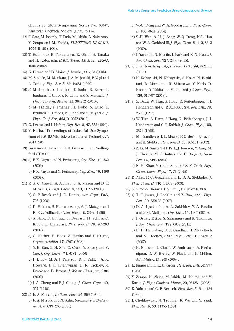
rials informatics, we must consciously practice the man-

ner of thinking based on data-oriented science. Not only

must we continue to improve our elemental technolo-

gies that we have accumulated thus far, but we must

also accelerate our efforts in new frontiers such as mate-

rials informatics.

Acknowledgment

The organic semiconductor analysis cases described

in the first half of Section 2 of Chapter 2 of this paper

were obtained from the 2013 industrial use of TSUB-

AME of the Tokyo Institute of Technology, subject num-

ber 13IBG. Also, the application examples of the K com-

puter described in Section 3 of Chapter 2 of this paper

were obtained through the use of the K computer of the

National Research and Development Agency RIKEN

(subject numbers: hp120028 and hp140089).

References

1) “Keisan no Kagaku in Iwanami Lecture Series

Keisan Kagaku”, Vol.1, A. Ukawa, A. Oshiyama, Y.

Oyanagi, M. Sugihara, A. Sumi and H. Nakamura

eds., Iwanami Shoten, p.3 (2013).

2) a) T. Nishikawa, Joho Kanri, 55(12), 882 (2013).

b) Research Organization for Information Science

and Technology, General Incorporated Founda-

tion, “Guide to HPCI for Beginner Users”,

http://www.hpci-office.jp/pages/e_guide (refer

at April. 16, 2015).

3) C. Hansch and T. Fujita, J. Am. Chem. Soc., 86, 1616

(1964).

4) O. Kirino, J. Pestisc. Sci. 9, 571 (1984).

5) C. Takayama, Y. Miyashita, S. Sasaki and M.Yoshida,

Quant. Struct.-Act. Relat., 2, 121 (1983).

6) M. Yoshida, J. Syn. Org. Chem., Jpn. 42, 743 (1984).

7) Y. Kurita, K. Tsushima and C. Takayama, “Probing

Bioactive Mechanisms (ACS Symposium Series

No.413)”, American Chemical Society (1989), p.183.

8) T. Katagi and Y. Kurita, J. Pestic. Sci., 14, 93 (1989).

9) K. Watanabe, K. Umeda, Y. Kurita, C. Takayama and

M. Miyakado, Pestic. Biochem. Physiol., 37, 275

(1990).

10) Y. Kurita, C. Takayama, T. Katagi and M. Yoshida,

“Computer Aided Innovation of New Materials”,

Elsevier Science (1991), p.455.

11) C. Takayama, N. Meki, Y. Kurita and H. Takano,

“Classical and Three-Dimensional QSAR in Agro-

For the SP estimation, we will improve the calculation

speed and accuracy and examine the MD calculation

with more consideration for structural parameters such

as an ordered structure. Moreover, we will investigate

the solubility predictive equation including solubility-

related parameters other than the SP.

Conclusion

U.S. President Barack Obama, in 2011, issued the

Materials Genome Initiative under the slogan of “2X

faster & 2X cheaper” in order to enhance the competing

power of the U.S. industry.48) In regard to the initiative

it was pointed out that it usually takes approximately 10

to 20 years from developing a material to launching it

into the market as a final product. In order to shorten

this process as much as possible, the materials infor-

matics approach is attracting much attention. The mate-

rials informatics procedures are as follows: Characteris-

tics that are unique to the material are calculated using

a computer simulation beforehand; the results of this

calculation are accumulated as a data set together with

the corresponding experimental data; and the structure

that realizes the target characteristics and functions is

derived from the above data set.49) While in the deduc-

tive approach one attempts to design a material having

the target functions by understanding and predicting the

material properties through experiments and theoretical

calculations using model structures, in materials infor-

matics an inductive approach is taken as follows: An

enormous data set of material characteristics is analyzed

through the informatics method, and a material having

the target functions is discovered based on the knowl-

edge obtained from that analysis.

Although in the beginning of this paper we stated that

computational science is considered as a “third science,”

such data-oriented science is currently advocated as a

“fourth science,” which covers a broader area. In the

field of materials science, this data-oriented science has

become mainstream in accelerating the movement of

materials informatics in terms of how (and how quickly)

we can discover the optimal combination from numer-

ous material-composition combinations.

In the previous chapter we introduced four cases with

a focus on our practical approach toward computational

materials science in electronics materials development

at Sumitomo Chemical. Our efforts remain within the

framework of the deductive approach. We believe that

in order to achieve an inductive approach such as mate-



c) W.-Q. Deng and W. A. Goddard III, J. Phys. Chem.

B, 108, 8614 (2004).

d) S.-H. Wen, A. Li, J. Song, W.-Q. Deng, K.-L. Han

and W. A. Goddard III, J. Phys. Chem. B, 113, 8813

(2009).

e) I. Yavuz, B. N. Martin, J. Park and K. N. Houk, J.

Am. Chem. Soc., 137, 2856 (2015).

23) a) J. E. Northrup, Appl. Phys. Lett., 99, 062111

(2011).

b) H. Kobayashi, N. Kobayashi, S. Hosoi, N. Koshi-

tani, D. Murakami, R. Shirasawa, Y. Kudo, D.

Hobara, Y. Tokita and M. Itabashi, J. Chem. Phys.,

139, 014707 (2013).

24) a) S. Datta, W. Tian, S. Hong, R. Reifenberger, J. I.

Henderson and C. P. Kubiak, Phys. Rev. Lett., 79,

2530 (1997).

b) W. Tian, S. Datta, S.Hong, R. Reifenberger, J. I.

Henderson and C. P. Kubiak, J. Chem. Phys., 109,

2874 (1998).

c) M. Brandbyge, J.-L. Mozos, P. Ordejón, J. Taylor

and K. Stokbro, Phys. Rev. B, 65, 165401 (2002).

d) Z. Li, M. Smeu, T.-H. Park, J. Rawson, Y. Xing, M.

J. Therien, M. A. Ratner and E. Borguet, Nano

Lett. 14, 5493 (2014).

e) K. H. Khoo, Y. Chen, S. Li and S. Y. Quek, Phys.

Chem. Chem. Phys., 17, 77 (2015).

25) P. Prins, F. C. Grozema and L. D. A. Siebbeles, J.

Phys. Chem. B, 110, 14659 (2006).

26) Sumitomo Chemical Co., Ltd., JP 2012-241038 A.

27) a) T. Fujiwara, J. Locklin and Z. Bao, Appl. Phys.

Lett., 90, 232108 (2007).

b) D. A. Lyashenko, A. A. Zakhidov, V. A. Pozdin

and G. G. Malliaras, Org. Elec., 11, 1507 (2010).

c) I. Osaka, T. Abe, S. Shinamura and K. Takimiya,

J. Am. Chem. Soc., 133, 6852 (2011).

d) B. H. Hamadani, D. J. Gundlach, I. McCulloch

and M. Heeney, Appl. Phys. Lett., 91, 243512

(2007).

e) H. N. Tsao, D. Cho, J. W. Andreasen, A. Rouha-

nipour, D. W. Breiby, W. Pisula and K. Müllen,

Adv. Mater., 21, 209 (2009).

28) E. Runge and E. K. U. Gross, Phys. Rev. Lett. 52, 997

(1984).

29) Y. Zempo, N. Akino, M. Ishida, M. Ishitobi and Y.

Kurita, J. Phys.: Condens. Matter, 20, 064231 (2008).

30) K. Yabana and G. F. Bertsch, Phys. Rev. B, 54, 4484

(1996).

31) J. Chelikowsky, N. Troullier, K. Wu and Y. Saad,

Phys. Rev. B, 50, 11355 (1994).

chemistry (ACS Symposium Series No. 606)”,

American Chemical Society (1995), p.154.

12) F. Goto, M. Ishitobi, T. Endo, M. Ishida, A. Nakazono,

Y. Zenpo and M. Yosida, SUMITOMO KAGAKU,

1994-@, 50 (1994).

13) T. Kunimoto, R. Yoshimatsu, K. Ohmi, S. Tanaka

and H. Kobayashi, IEICE Trans. Electron., E85-C,

1888 (2002).

14) G. Bizarri and B. Moine, J. Lumin., 115, 53 (2005).

15) M. Städele, M. Moukara, J. A. Majewski, P. Vogl and

A. Görling, Phys. Rev. B, 59, 10031 (1999).

16) a) M. Ishida, Y. Imanari, T. Isobe, S. Kuze, T.

Ezuhara, T. Umeda, K. Ohno and S. Miyazaki, J.

Phys.: Condens. Matter, 22, 384202 (2010).

b) M. Ishida, Y. Imanari, T. Isobe, S. Kuze, T.

Ezuhara, T. Umeda, K. Ohno and S. Miyazaki, J.

Phys.: Conf. Ser., 454, 012062 (2013).

17) G. Kresse and J. Hafner, Phys. Rev. B, 47, 558 (1999).

18) Y. Kurita, “Proceedings of Industrial Use Sympo-

sium of TSUBAME, Tokyo Institute of Technology”,

2014, 203.

19) Gaussian 09, Revision C.01, Gaussian, Inc., Walling-

ford CT, 2009.

20) a) P. K. Nayak and N. Periasamy, Org. Elec., 10, 532

(2009).

b) P. K. Nayak and N. Periasamy, Org. Elec., 10, 1396

(2009).

21) a) S. C. Capelli, A. Albinati, S. A. Mason and B. T.

M. Willis, J. Phys. Chem. A, 110, 11695 (2006).

b) C. P. Brock and J. D. Dunitz, Acta Cryst., B46,

795 (1990).

c) D. Holmes, S. Kumaraswamy, A. J. Matzger and

K. P. C. Vollhardt, Chem. Eur. J., 5, 3399 (1999).

d) S. Haas, B. Batlogg, C. Besnard, M. Schiltz, C.

Kloc and T. Siegrist, Phys. Rev. B, 76, 205203

(2007).

e) C. Näther, H. Bock, Z. Havlas and T. Hauck,

Organometallics, 17, 4707 (1998).

f) Y.-H. Sun, X.-H. Zhu, Z. Chen, Y. Zhang and Y.

Cao, J. Org. Chem., 71, 6281 (2006).

g) P. J. Low, M. A. J. Paterson, D. S. Yufit, J. A. K.

Howard, J. C. Cherryman, D. R. Tackley, R.

Brook and B. Brown, J. Mater. Chem., 15, 2304

(2005).

h) J.-A. Cheng and P.-J. Cheng, J. Chem. Cryst., 40,

557 (2010).

22) a) R. A. Marcus, J. Chem. Phys., 24, 966 (1956).

b) R. A. Marcus and N. Sutin, Biochimica et Biophys-

ica Acta, 811, 265 (1985).



43) K. L. Hoy, J. Paint. Technol., 42, 76 (1970).

44) J. Brandrup, E. H. Immergut and E. A. Grulke,

“Polymer Handbook 4th”, Wiley (2003).

45) H. Ebata, T. Izawa, E. Miyazaki, K. Takimiya, M.

Ikeda, H. Kuwabara and T. Yui, “J. Am. Chem. Soc.,

129, 15732 (2007).

46) T. Okamoto, C. Mitsui, M. Yamaguchi, K. Nakahara,

J. Soeda, Y. Hirose, K. Miwa, H. Sato, A. Yamano, T.

Matsushita, T. Uemura and J. Takeya, Adv. Mater.,

25, 6392 (2013).

47) Sumitomo Chemical Co., Ltd., JP 2009-267372A

(2009), JP 5480510 B2 (2014).

48) the WHITE HOUSE PRESIDENT BARACK

OBAMA, “Materials Genome Initiative for Global

Competitiveness, June 2011”, https://www.

whitehouse.gov/sites/default/files/microsites/

ostp/materials_genome_initiative-final.pdf (Ref.

2015/4/16).

49) Center for Research and Development Strategy,

Japan Science and Technology Agency, “STRATE-

GIC PROPOSAL; Materials Informatics Materials

Design by Digital Data Driven Method.” (2013),

http://www.jst.go.jp/crds/pdf/2013/SP/CRDS-

FY2013-SP-01.pdf (refer at April 16, 2015).

32) M. Ishida, N. Akino, Y. Zempo, S. Urashita, S. Shingu,

H. Suno and N. Nishikawa, “The User Report of the

Earth Simulator Industrial Application Project”, p.29

(2010).

33) Y. Zempo, N. Akino, M. Ishida, E. Tomiyama and H.

Yamamoto, J. Phys. Conf. Series, in submitted.

34) M. Ishida, “HPCI User Report for Industrial Use

of K computer, 2013”, https://www2.hpci-office.jp/

output/hp120028/outcome.pdf (refer at April 16,

2015).

35) S. Kuroda, OYOBUTSURI, 76, 795 (2007).

36) H. Masuhara, Polymers, 60, 53 (2011).

37) S. Habuchi and M. Vacha, Polymers, 60, 54 (2011).

38) J. H. Hildebrand and R. L. Scott, “The Solubility

of Non-Electrolytes”, Reinhold Publishing Corp.

(1949).

39) P. A. Small, J. Appl. Chem, 3, 77 (1953).

40) R. F. Fedors, Polym. Eng. Sci., 14, 147&472 (1974).

41) D.W. Van Krevelen and P. J. Hoftyzer, “Properties of

Polymers, Their Estimation and Correlation with

Chemical Structure”, Elsevier Publishing Company,

Amsrerdam (1972).

42) C. M. Hansen, “Hansen Solubility Parameters”, CRS

Press (2000).

P R O F I L E

Masaya ISHIDA

Sumitomo Chemical Co., Ltd.Advanced Materials Research LaboratorySenior Research Associate

Akiko NAKAZONO

Sumitomo Chemical Co., Ltd.Advanced Materials Research LaboratorySenior Research Specialist

Yasuyuki KURITA

Sumitomo Chemical Co., Ltd.Advanced Materials Research LaboratorySenior Research Specialist, Doctor of Agriculture

Documents

Materials Design and Prediction Using Computational Science · band calculation in order to obtain the optical band gap. The optical band gap was estimated using the energy difference