Matching Revenues and Costs: The Counter-Intuitive

International Journal of Business and Management; Vol. 15, No. 1; 2020 ISSN 1833-3850 E-ISSN 1833-8119

Published by Canadian Center of Science and Education

202

Matching Revenues and Costs: The Counter-Intuitive Rationality of Direct Costing

Anna Maria Moisello1 & Piero Mella1 1 Department of Economics and Management, University of Pavia, Pavia, Italy Correspondence: Anna Maria Moisello Department of Economics and Management, University of Pavia, Pavia, Italy. E-mail: [email protected]

Received: November 29, 2019 Accepted: December 21, 2019 Online Published: December 30, 2019

doi:10.5539/ijbm.v15n1p202 URL: https://doi.org/10.5539/ijbm.v15n1p202 Abstract This study investigates the consequences of adopting two simple sets of rules the manager can consider as perfectly rational and follow in his decisions regarding price, volume and mix of the various products. The first set follows the full (absorption) costing method logic, while the second is based on the direct (variable, marginal) costing method logic. It shows that costing systems adopting the full-costing method can lead management to make non-rational decisions regarding the setting of prices, acceptance of orders, make or buy choices and, above all, determination of the optimal production mix through programming and budgeting. On the other hand, using the direct costing method allows the manager to achieve rational results during the decision-making and planning phases, even if these often appear counter-intuitive when compared with the results achieved using the full costing method, which seem to conform to naïve intuition. The risk in the latter case is even more serious when we are dealing with multi-production firms operating under conditions of limited production capacity regarding one or more factors, as occurs most of the time. The demonstration of the thesis of the superiority of direct costing method rules in management decisions related to the problem of the matching costs and revenues is carried out with numerical evidence, formulating a set of decision problems that are solved by comparing the results obtained both with the full costing method rules and with the direct costing method rules. Keywords: direct costing method, full costing method, linear programming, management decisions 1. Introduction Managerial choices assume a countless number of valuation processes. The principle of managerial activity aimed at guiding the business system toward its objectives in itself implies the search for accurate control strategies (Mella, 2014). The economic value of a firm (EVF) expresses the main business and managerial objective whose achievement requires a strategy that, for the different business segments, correctly calculates costs, prices, volumes and production mix in order the quantify the maximum return on investment (roi), which is a prerequisite for achieving the maximum return on equity (roe), on which EVF depends (Mella, 2005, 2014; McIntyre, 1999). Each technical control of roi is mainly based on price and cost control, with business, marketing and industrial policies affecting quality and productivity (Mella, 2018a, 2018b). In particular, the ‘heart’ of any strategy to control the return on invested capital, roi, in multi-product companies must decide how to correlate in a meaningful manner sales revenues and production costs, in order to calculate the analytical economic results for each type of production so as to decide the optimal production mix, and which products to start, continue or interrupt producing. In addition, it must monitor the production volumes of each product. This strategic problem appears even more relevant when there are production or resource capacity constraints. Usually the debate between full costing and direct costing advocates revolves around the cost accounting systems with respect to both the evaluation of inventories and the ex post calculation of economic results in financial statements. The present study instead examines the two cost methods from an operational and managerial point of view, since they can deal with and solve in different ways the fundamental problems of any business strategy: how to rationally correlate prices and costs, on which some fundamental choices depend. For planning and budgeting purposes (Sponem, 2016; Hansen, 2004), the most relevant of these decisions concern: – How to set profitable prices on the basis of the unit cost data and, vice-versa: what target costs must be achieved given the pre-determined prices;

ijbm.ccsenet.org International Journal of Business and Management Vol. 15, No. 1; 2020

203

– Whether or not to activate or de-activate a production process, given the estimated selling prices; – Which product mix is most rational given the selling prices and unit costs of production. Today, management accounting can rely on a considerable variety of systems for calculating the costs of production (Moisello, 2000; Avi, 2012, Ogungbade & Tabhita, 2018): from the simple one-step calculation methods, which attempt to impute to products the costs of all the productive factors by employing mainly volumetric cost drivers, to the multi-step methods, such as “localization method” which operates through the allocation of elementary costs to cost centers, and activity based costing, or ABC, that allocates elementary costs based on the activities necessary for the production processes (Homburg, 2001; Cooper, 1988a, 1988b; Cooper & Kaplan, 1991; Bhimani & Pigott, 1992; Dugdale & Jones, 1997; Mitchell, 1994). These systems attribute the costs of factors of production (first step) first to the operational centers (localization) or the activities (ABC) and subsequently, after a certain number of exchanges among centers or between activities and macro activities (further steps), to the finished product (final step), using appropriate cost drivers that ensure an imputation based on assumed causal relations that link the activities to the finished products (Moisello, 2012a). Common to these systems is the fact that, more or less explicitly, they adopt the full cost method (logic) of calculation; that is, the logic of the full costing method (Kaplan and Johnson, 1987). Full costing represents the cost of all the factors – whether involved in the process or capacity, technical or financial, or effective or figurative in nature – held to contribute to obtaining a given volume of production. Precisely because it represents the economic consumption of all the factors, full costing is highly meaningful in terms of the efficiency of production processes and commonly used, having become by now the ‘king of the market’. The full costing method is also found in the target costing process, a system of cost management and planning regarding the production mix that aims at maximizing profitability (Moisello, 2012b; Ansary & Bell, 1997; Kato, 1993), taking the selling price as a constraint and trying to redesign the production process in order to keep costs at a level that, given the price constraint, produces the desired profitability. Finally, though this does not exhaust the varieties of costing systems, there is the Life Cycle Costing technique (Cooper & Chew, 1996), which determines the cost limits of a product in the various stages of its life cycle, with the aim of determining the moment of optimal conclusion of the life cycle to avoid the cash cow being transformed into a cash dog, according to the Boston Consulting Group framework. What is the reason for bringing up the direct costing method? For the answer, it is necessary to note that the cost calculations are part of the managerial calculations of economic effectiveness, which as a whole are referred to as the economic and productive calculation (Mella, 2005). In particular, the ‘heart’ of the economic calculation undertaken in multi-product companies attempts to correlate in a meaningful manner sales revenues and production costs, in order to calculate the analytical economic results for each type of production so as to decide which production to start, continue or interrupt and to monitor the carrying out of the production processes. The system of calculations of production costs must be suitable to the carrying out of a rational economic calculation (Cooper & Kaplan, 1988a, 1988b). From this perspective, a costing system can be defined as appropriate and coherent if it allows management to make the most rational decisions regarding profitability, thereby allowing costs and prices to be correlated so as to maximize the product mix given the constraint of obtaining the maximum revenue. This paper aims at demonstrating how the full costing method can distort operating decisions, as it assumes the imputation of all costs to the pre-determined production volumes, both direct and indirect costs, that can change only in the long term and do not affect this kind of decisions,. No matter how production is implemented: through cost centers, or through activities or processes, it can lead to non-rational operating decisions since it does not focus on relevant costs (Staubus, 1963) and it does not optimize the economic results that can be achieved. Only the direct costing method, since it investigates the dynamics of factor costs according to the dynamics of production volumes, dividing these into variable, direct (hence the term “direct” costing), and fixed costs, allows for the proper determination of the production mix to achieve maximum profitability. The direct costing method therefore refers to the calculation of costs at variable volumes of production and no longer only to "fixed" production volumes; in other words, the economic result for each production process becomes a function of the revenues, prices and volumes, and of the variable and fixed costs, for each level of production. Referring to a number of numerical examples, this paper highlights that the direct costing method can be defined as appropriate and coherent since it allows management to make the most rational decisions regarding profitability, thereby allowing costs and prices to be correlated so as to maximize the product mix given the constraint of obtaining the maximum revenue. More specifically, adopted as a decision-making criterion, the direct costing method consistently produces optimal results, even if in some cases these appear counter-intuitive.


204

Nevertheless, when compared with alternative results from the full costing method, the former turn out to be perfectly rational. 2. Full and Direct Costing: A Short Literature Review The development of cost accounting and managerial control dates to the beginning of the 19th century, when companies began to hire workers on a long-term basis and to realize the need to operate according to efficiency criteria (Johnson & Kaplan, 1987). Another strong incentive for the development of cost accounting techniques occurred in the second half of the 19th century, when the management of large transport, production and distribution companies felt the need for cost information useful to support business operations and growth processes (Waweru, 2010). Nevertheless, Kaplan (1984) observed that over the entire century cost accounting practices did not allocate fixed costs either to periods or to products, a practice that was begun by scientific management. Moss and Haseman (1957) point out that the development of the principle of burden application can be considered as the antecedent of direct costing. This approach recognizes that certain costs are not related to a specific output but to supply services beyond a single accounting period, therefore implying above all a cost allocation among different accounting periods and subsequently an allocation among different outputs. As the authors highlight, the fluctuations of outputs and costs reduce the validity of full cost information for the decision-making process. The full costing school, acknowledging the aforementioned limitations, refined the methodology by basing burden rates on the normal activity level or on the level related to practical capacity. The costs allocated in this way take on the meaning of “unavoidable amount of overhead cost” attributable on average to a single product unit, under the assumption that the company operates at the level of activity assumed as the basis for determining the allocation coefficient (Moss & Haseman, 1957 p. 185). Conversely, the direct costing school proposed to treat the amount of overhead cost not related to a specific output as period costs and not as product costs. Subsequently, the identification of the cost to be allocated to the product based on the direct relationship with the output was refined by taking into account the variability of the cost. Direct costing has its roots on management’s need for quantitative information on the effect of the cost-volume-price relationship on a business (Moss & Haseman, 1957). Many authors have emphasized the operational importance of the choice between full and direct costing in managerial decisions. The literature points out a number of concerns related to the use of absorption costing in profitability analysis, which is key for many decisions such as the elimination of products, the prioritization of products for sales activities, the determination of the optimum mix of production, and sales planning for products, suggesting the use of information based on variable costs, taking into account production constraints (Guerreiro et al., 2004). The advantages of contribution margin information in pricing decisions were effectively highlighted by Horngren, (1972), and the literature has consistently proposed models for pricing and profitability decision-making based on variable costs and contribution margin. The literature observes that the allocation of fixed costs to products may lead to adverse decision-making because the value attributed to a unit depends on the production volume as well as on the allocation criterion adopted (Guerreiro et al., 2004). Conversely, the contribution margin highlights in an unbiased way how the different products contribute to covering the structure costs and to producing profit. Noreen, Smith and Mackey (1995) point out that the contribution margin per unit of a constraint resource is a key indicator in deciding how to optimize its use or whether to elevate the constraint. Nevertheless, the full costing method has been indicated as an effective tool in dealing with the complexity of triple bottom line decisions; in particular, for businesses characterized by relevant environmental and social implications such as the automotive industry (Jasinski et al., 2015). The method has been applied to incorporate in products prices the value of internal and external impacts in order to pursue the overall sustainability of a business (Bebbington, 2001). Valuations of product stocks for external financial reporting is another significant point in the debate on the choice between full costing and direct costing (Moisello, 2000). Advocates of direct costing assessment note that fixed costs occur regardless of production volumes and of the production of products in stock. Therefore, these costs should not be transferred to the future financial year by the value assigned to inventories (Horngren & Sorter,1961). The proponents of direct costing argue that the result for the year would be clearer and more meaningful, since it does not depend on production volumes and is influenced solely by sales volume. Those who opt for full costing emphasize that structural factors are indispensable for obtaining production and that the related costs must be taken into account in the assessment of stocks. In doing so, the portions of fixed costs as well are postponed to the year in which the sales are made, perfectly matching revenues and costs (Paton & Littleton, 1940; Fremgen, 1964), while idle capacity costs should be treated as losses (Fess & Ferrara, 1961).


205

The empirical literature on the measurement of the economic results and the significance of financial statements (Pong & Mitchel, 2006) highlights that the choice between full costing and direct costing is relevant since these two methods provide different profit measurements when a variation between the stocks at the beginning and end of the period occurs. Under absorption costing the increase of stocks enhances profit, with some authors pointing out that the full costing method may motivate managers to increase stocks in order raise profit (Kaplan, 1984; Johnson & Kaplan, 1987). Conversely, in accounting frameworks, such as GAAP and IFRS, variable costing is not allowed in financial reporting and absorption costing is mandatory (Krishnan & Lin, 2012) since it is assumed that this accounting principle refers to historical periods in which the actual production data is known. In accordance with the accounting standards for external financial reporting, the cost of inventory must be determined in accordance with the matching principle in accounting, which requires expenses to be reported in the same period as the revenue generated by the expenses, including all costs used to prepare the inventory for its intended use. 3. The Logic of the Full (Absorption) Costing Method in Management Accounting As mentioned in Section 1, today, management accounting can rely on a considerable variety of systems for calculating the costs of production (Moisello, 2000; Drury, 2013): from the simple one-step calculation methods, which attempt to impute to products the costs of all the productive factors by mainly employing volumetric cost drivers, to the multi-step methods, such as localization and activity based costing (ABC). These systems attribute the costs of factors of production (first step) first to the operational centers (localization) or the activities (ABC) and subsequently, after a certain number of exchanges among centers or between activities and macro activities (further steps), to the finished product (final step), using appropriate cost drivers that ensure an imputation based on assumed causal relations that link the activities to the finished products (Moisello, 2012c). Common to these systems is the fact that, more or less explicitly, they adopt the full cost method (logic) of calculation. Full costing represents the cost of all the factors – involved in the process or in production capacity, and technical or financial, effective or figurative in nature – that are held to contribute to obtaining a given volume of production. Precisely because it represents the economic consumption of all the factors, full costing is highly meaningful in terms of the efficiency of production processes and commonly used, by now having become the ‘king of the market’. The full costing method is also found in the target costing process, a system of cost management and planning regarding the production mix that aims at maximizing profitability taking the selling price as a constraint and trying to redesign the production process in order to keep costs at a level that, given the price constraint, produces the desired profitability. Finally, though this does not exhaust the varieties of costing systems, there is the Life Cycle Costing technique which determines the cost limits of a product in the various stages of its life cycle, with the aim of determining the moment of optimal truncation of the life cycle in order to avoid the cash cow being transformed into a cash dog, according to the framework of the Boston Consulting Group. What is the reason for bringing up the direct costing method? For the answer it is necessary to note that the cost calculations are part of the managerial calculations of economic effectiveness, which as a whole are referred to as the economic and productive calculation (Mella, 1997). 4. From Management Accounting to the Management Problem of Correlating Unit Costs and Prices Dealing with the problem of the correlation between revenues and costs means in practice solving the problem of how to meaningfully compare prices and unit costs (Moyer et al., 2014) in production and pricing decisions: in other words, how to establish, for example, if it is economically convenient to produce the product ALFA, for which a client offers to pay 5 euros per unit, with a cost of 5.4 euros per unit; or when should it be decided which of the two products, BETA and GAMMA, to produce, given an offering price of 10 and 20 euros, respectively, and a unit cost of 8 and 19 euros. It may sound incredible, but the intuitive answers «do not produce ALFA, as this will entail a loss for each unit» and «produce BETA, since this offers a higher profit per unit» could turn out to be wrong and lead as a result to a reduction in overall economic efficiency and results. For this reason, the correct procedure management adopts to correlate costs/prices is fundamental for the very survival of the company, especially in multi-process and multi-product corporations. To demonstrate this, we must compare the analyses of the two costing methods; that is, the two methods for correlating unit costs and prices, and as a result total costs and revenues (Rajasekaran & Lalitha, 2011). In single-product companies the correlation between costs and revenues for a given production process is correctly achieved using the method knows as break-even analysis (BEA) (Cafferky, 2010), which analyzes the dynamics of costs and revenues as a function of the quantity produced by that process. In this way the


206

corresponding operating result for each level of production is determined, which is also a function of the volumes of production and sales (referring as it does to a production process, the stock of products is irrelevant). BEA thus assumes the possibility of specifying the economic result functions, by deriving these from the cost, earnings and operating results functions with respect to the quantity to produce as the independent variable (DuBrin, 2008). In its traditional form, the BEA is based on the fundamental hypothesis that revenues and costs vary linearly with respect to variations in the quantity produced and sold, Q. This simply means that the operational result function (R), considering the production volumes Q as an independent variable, take the following form:

( ) CF - Q FCQ Q R(Q) cmvcp =+−= (1)

This represents the fundamental expression of BEA in a linear form, since: • vc = Σ qV pV is the unit variable cost, obtained from the sum of the variable costs (qV pV) of the direct operating factors; that is, the costs for materials, services and direct labor – whose total increases with increases in the volumes (Q) of production – which are calculated by multiplying the unit quantities of the factors (qV) by the unit prices (pV); VC = vc Q represents the total variable costs function, since the costs for the operating factors are the costs for production, and therefore vary along with variations in the latter; they can also be called the “costs of the production process”; • FC = Σ qF pF are the total fixed costs for the process, and represent the sum of the costs of fixed structures (qF pF) – quantity (qF) multiplied by unit prices (pF) – that is, the costs for machinery and facilities, or the depreciation, rent, and so on, borne in a given amount independently of the volume of production; FC are also called “costs of production structures”, or simply “structure costs”. If these refer to a process lasting one year, they are also called “period costs”. Since BEA is applied linearly, all the basic costs that are not linear must be “linearized”: their dynamics, whatever form this should take, must be reduced to a linear form through appropriate procedures (see Mella 1997). From (1) it follows that, following the BEA logic, when Q = 0, the cost of production is equal to FC. The cost-price correlation through (1) allows us to correctly calculate the volume Q* which, given p, vc and FC, gives us a desired R*; in fact, we immediately derive the following fundamental equation of the BEA:

cmvcp*RFC*RFCQ* +=

−+= (2)

Where the denominator (p-vc) represents the unit contribution margin, cm, to cover fixed costs and achieve the desired level of operational result. The quantity Qe that achieves equilibrium is the “equilibrium quantity”, which corresponds to the production volume at which total costs equal total revenues, known as the break-even quantity or, more briefly, break-even point (BEP). Since costs are a function of Q, for every level of Q we can quantify the average relative cost, or unitary full cost:

QFCQ += vcfc (3)

Given the presence of fixed costs, fc will decline with increases in the volumes of production. It must be noted that in normal circumstances Q does not vary from zero to infinity, since for levels that are “too small”, near to zero, all costs have anomalous trends which are not easily determinable. Similarly, for production quantities that are ‘too high’, costs cannot be quantified. For this reason, in BEA the quantity Q varies from a minimum volume to a maximum volume in the “neighborhood” of a normal volume of production: the “admissible neighborhood” (range of admissible variability), which is assumed to be obtained without variations in production capacity. While the BEA allows us to solve the problem of the cost/price correlation in a single product company, in multi-product companies the correlation between specific sales revenues and specific production costs, needed to quantify the analytical results, can be found using the full cost method, better known as the full costing method, and the variable direct cost method, better known as the direct costing method, or also the variable costing method. The two methods assume the possibility of constructing the cost functions for each production process according to the BEA techniques, quantifying the revenues, costs, and results based on a given normal quantity of production, and constructing an analytical accounting matrix in which for each product, placed at the top of separate column, volumes, prices and costs are calculated in the corresponding rows. We can now move on to an


207

analysis of the full cost or full costing methods as alternative price/cost decision-making criteria. 5. The Full Costing Method Rules to Compare Unitary Costs and Prices According to this method, the price/cost comparison must involve the selling price (p), with full cost defined as the overall average unit cost, which includes both the unit variable costs (vc) as well as a unit share of the fixed costs, which will be indicated by the symbol fc (note: FC indicates total fixed costs; fc is the share of these costs attributed to each unit of product) (Gramlich & Korok 2015). Therefore, indicating unitary full cost by “fc”, and keeping in mind (3), we can write:

fcvcvcfc +=+=QFC (4)

From (4) we see that unit fixed costs (cf) are determined by dividing overall fixed costs by the normal quantity Q. The value ‘fc’ represents full cost, since it is the unit cost that includes both the share of variable costs and that part of fixed costs imputed to each unit of production. This method thus assumes that each unit of production obtained and sold must also absorb a share of the fixed costs needed for production, in addition to covering the variable costs vc. Therefore, the full costing method is also known as the absorption costing method (Drury, 2013). Using the usual symbols, the difference between “p” and “fc” measures the unit result “ur”; that is, the unit profit or unit loss:

( )fcvcpfcpur −−=−= (5)

This leads to the following operating rule for managerial economic calculations regarding the comparison of the unit price/cost with the full costing method: Rule 1): a product whose selling price “p” is below full cost, “fc”, should not be produced, since the price does not cover the production costs, and thus manufacturing it would inevitably lose money for the company;

Rule 2): as a result of Rule 1, the relation p > vc +fc must always hold; Rule 3): when there are two products with different unit profits, a company must favor the most profitable one; that is, the one for which “ur” is greater. In particular, if the firm produces ALFA and BETA, the first with a unit profit and the second a unit loss, it must stop producing BETA in order to avoid losses. 6. Theoretical Analysis of Problems Arising from the Full Costing Method 6.1 Stopping Production of a Loss-Making Product: Single Production The rules of the full costing method can lead to non-rational decisions. To demonstrate this, we can begin with a simple proof. Let us assume a single-product company produces a “normal” quantity of ALFA equal to Q = 100,000 units, with variable costs vc = 31.50 and fixed costs FC = 2,000,000 (let us suppose that all values are in some form of money unit: € or $ or £, etc.). The selling price is p = 49 (all money values can be expressed in some money unit: € or $ or £, or another unit of currency). In order to judge whether it is economically convenient to produce according to RULES 1 and 2 above we need to calculate the full cost by first determining the fixed cost share, “fixed c”, absorbed by each unit of product and then adding these to the unit variable costs:

20.00100,000

2,000,000 ==cfixed

The unit full cost is: 51.5020.0031.50 =+=+= cfixedvcfc

Since the price is p = 49, which is below unit full cost, it must be deduced that the production of ALFA is not economically convenient, since for each unit of production there would be a negative result, a loss, in the amount of:

2.5051.5049.00 −=−=−= fcpur (loss per unit). We assume that management, having observed this result, decides to interrupt production of ALFA. Is this a rational decision? To answer this, we need further information about the following two possibilities: whether the can company replace the production of ALFA with another, or whether it must stop producing ALFA without


208

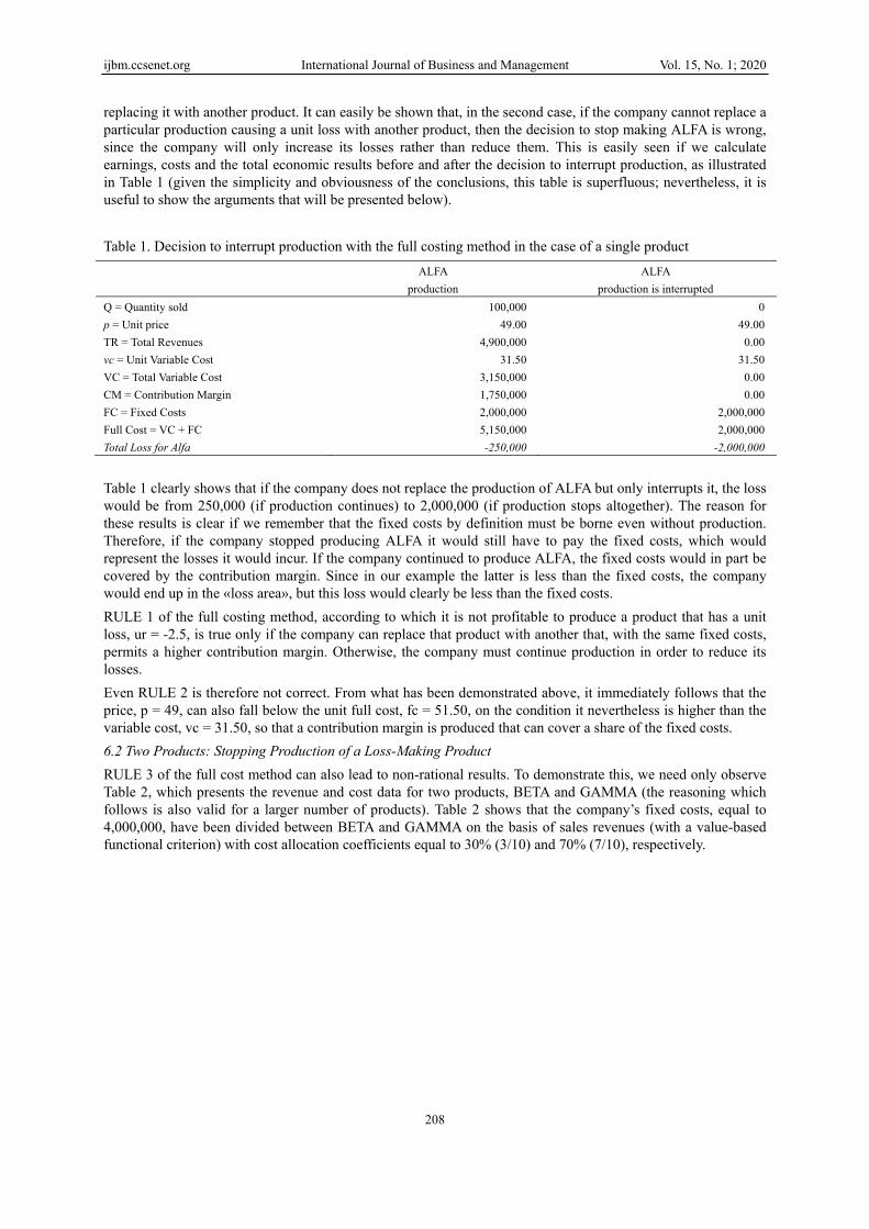
replacing it with another product. It can easily be shown that, in the second case, if the company cannot replace a particular production causing a unit loss with another product, then the decision to stop making ALFA is wrong, since the company will only increase its losses rather than reduce them. This is easily seen if we calculate earnings, costs and the total economic results before and after the decision to interrupt production, as illustrated in Table 1 (given the simplicity and obviousness of the conclusions, this table is superfluous; nevertheless, it is useful to show the arguments that will be presented below). Table 1. Decision to interrupt production with the full costing method in the case of a single product ALFA

production ALFA

production is interrupted Q = Quantity sold p = Unit price TR = Total Revenues vc = Unit Variable Cost VC = Total Variable Cost CM = Contribution Margin FC = Fixed Costs Full Cost = VC + FC Total Loss for Alfa

100,000 49.00

4,900,000 31.50

3,150,000 1,750,000 2,000,000 5,150,000 -250,000

0 49.00

0.00 31.50

0.00 0.00

2,000,000 2,000,000

-2,000,000 Table 1 clearly shows that if the company does not replace the production of ALFA but only interrupts it, the loss would be from 250,000 (if production continues) to 2,000,000 (if production stops altogether). The reason for these results is clear if we remember that the fixed costs by definition must be borne even without production. Therefore, if the company stopped producing ALFA it would still have to pay the fixed costs, which would represent the losses it would incur. If the company continued to produce ALFA, the fixed costs would in part be covered by the contribution margin. Since in our example the latter is less than the fixed costs, the company would end up in the «loss area», but this loss would clearly be less than the fixed costs. RULE 1 of the full costing method, according to which it is not profitable to produce a product that has a unit loss, ur = -2.5, is true only if the company can replace that product with another that, with the same fixed costs, permits a higher contribution margin. Otherwise, the company must continue production in order to reduce its losses. Even RULE 2 is therefore not correct. From what has been demonstrated above, it immediately follows that the price, p = 49, can also fall below the unit full cost, fc = 51.50, on the condition it nevertheless is higher than the variable cost, vc = 31.50, so that a contribution margin is produced that can cover a share of the fixed costs. 6.2 Two Products: Stopping Production of a Loss-Making Product RULE 3 of the full cost method can also lead to non-rational results. To demonstrate this, we need only observe Table 2, which presents the revenue and cost data for two products, BETA and GAMMA (the reasoning which follows is also valid for a larger number of products). Table 2 shows that the company’s fixed costs, equal to 4,000,000, have been divided between BETA and GAMMA on the basis of sales revenues (with a value-based functional criterion) with cost allocation coefficients equal to 30% (3/10) and 70% (7/10), respectively.


209

Table 2. Full costing method in the case of two products BETA

Production GAMMA

Production Totals

Q = Quantity sold p = Unit price TR = Total Revenues vc = Unit Variable Cost VC = Total Variable Cost CM = Contribution Margin FC = Fixed Costs Fixed Costs allocation coefficients (TR) Full Cost = VC + FC fc = unit full cost ur = unit result = p – fc R = Operating Income

100,00030.00

3,000,00015.00

1,500,0001,500,0001,200,000

30 %2,700,000

273

300,000

200,000 35.00

7,000,000 25.00

5,000,000 2,000,000 2,800,000

70 % 7,800,000

39 -4

-800,000

10,000,000

6,500,0003,500,0004,000,000

100 %10,500,000

-500,000 The unit full cost is:

27.0012.0015.00(BETA) =+=fc

39.0014.0025.00(GAMMA) =+=fc

Since the selling price of the two products is 30 and 35, respectively, the following unit results are obtained:

3.0027.0030.00(BETA) +=−=ur

4.0039.0035.00(GAMMA) −=−=ur According to full costing RULE 3, GAMMA production must be interrupted. This conclusion is clearly non-rational: it is not economically convenient for the company to replace a product with a unit loss unless the new product has a higher contribution margin. In fact, this would lead to a variant of the case mentioned in the previous section: as Table 3 illustrates, even if the company stops the production of GAMMA, all the fixed costs imputed to that production would still be incurred; and, not being able to count on the contribution margin from this production, the total loss would rise from 500,000 to 2,500,000. Table 3. Decision to stop production in the case of two products, under the full costing method

BETA Production

GAMMA Production

Totals

Q = Quantity sold p = Unit price TR = Total Revenues vc = Unit Variable Cost VC = Total Variable Cost CM = Contribution Margin FC = Fixed Costs Fixed Costs allocation coefficients (TR) Full Cost = VC + FC fc = unit full cost R = Operating Income

100,00030.00

3,000,00015.00

1,500,0001,500,0004,000,000

100%5,500,000

55.0-2,500,000

0 35.00

0 25.00

0 0 0 0 0 0 0

3,000,000

1,500,0001,500,0004,000,000

100%5,500,000

-2,500,000 This example leads to the following conclusion: the full costing method leads to non-rational decisions when there is unutilized production capacity; that is, when it must be decided whether or not to continue or interrupt a certain production without replacing that production with another; in other words, without covering the fixed costs imputed to the interrupted production (the case of fully utilized production capacity is dealt with in the next section).


210

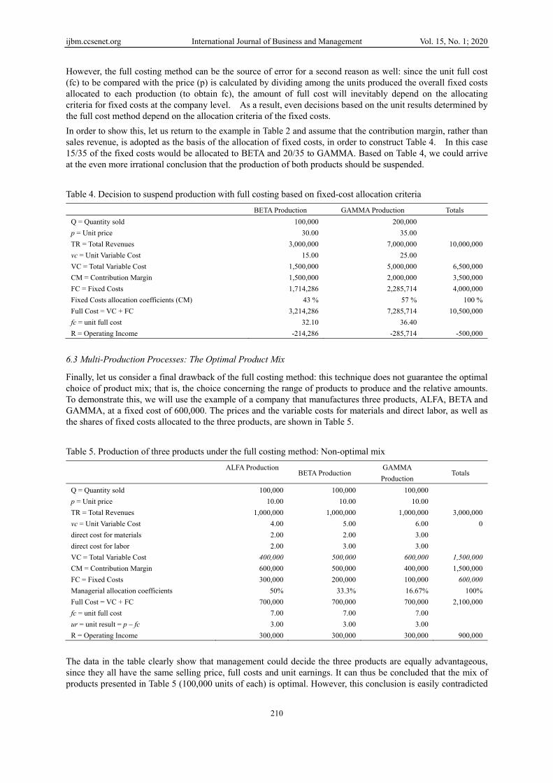
However, the full costing method can be the source of error for a second reason as well: since the unit full cost (fc) to be compared with the price (p) is calculated by dividing among the units produced the overall fixed costs allocated to each production (to obtain fc), the amount of full cost will inevitably depend on the allocating criteria for fixed costs at the company level. As a result, even decisions based on the unit results determined by the full cost method depend on the allocation criteria of the fixed costs. In order to show this, let us return to the example in Table 2 and assume that the contribution margin, rather than sales revenue, is adopted as the basis of the allocation of fixed costs, in order to construct Table 4. In this case 15/35 of the fixed costs would be allocated to BETA and 20/35 to GAMMA. Based on Table 4, we could arrive at the even more irrational conclusion that the production of both products should be suspended. Table 4. Decision to suspend production with full costing based on fixed-cost allocation criteria

BETA Production GAMMA Production Totals Q = Quantity sold p = Unit price TR = Total Revenues vc = Unit Variable Cost VC = Total Variable Cost CM = Contribution Margin FC = Fixed Costs Fixed Costs allocation coefficients (CM) Full Cost = VC + FC fc = unit full cost R = Operating Income

100,00030.00

3,000,00015.00

1,500,0001,500,0001,714,286

43 %3,214,286

32.10-214,286

200,000 35.00

7,000,000 25.00

5,000,000 2,000,000 2,285,714

57 % 7,285,714

36.40 -285,714

10,000,000

6,500,0003,500,0004,000,000

100 %10,500,000

-500,000 6.3 Multi-Production Processes: The Optimal Product Mix

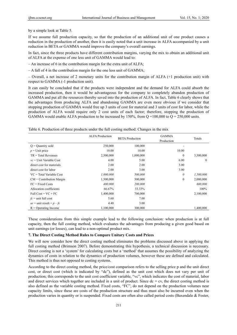
Finally, let us consider a final drawback of the full costing method: this technique does not guarantee the optimal choice of product mix; that is, the choice concerning the range of products to produce and the relative amounts. To demonstrate this, we will use the example of a company that manufactures three products, ALFA, BETA and GAMMA, at a fixed cost of 600,000. The prices and the variable costs for materials and direct labor, as well as the shares of fixed costs allocated to the three products, are shown in Table 5. Table 5. Production of three products under the full costing method: Non-optimal mix

ALFA Production BETA Production

GAMMA Production

Totals

Q = Quantity sold p = Unit price TR = Total Revenues vc = Unit Variable Cost direct cost for materials direct cost for labor VC = Total Variable Cost CM = Contribution Margin FC = Fixed Costs Managerial allocation coefficients Full Cost = VC + FC fc = unit full cost ur = unit result = p – fc R = Operating Income

100,00010.00

1,000,0004.002.002.00

400,000600,000300,000

50%700,000

7.003.00

300,000

100,00010.00

1,000,0005.002.003.00

500,000500,000200,000

33.3%700,000

7.003.00

300,000

100,000 10.00

1,000,000 6.00 3.00 3.00

600,000 400,000 100,000 16.67% 700,000

7.00 3.00

300,000

3,000,0000

1,500,0001,500,000

600,000100%

2,100,000

900,000 The data in the table clearly show that management could decide the three products are equally advantageous, since they all have the same selling price, full costs and unit earnings. It can thus be concluded that the mix of products presented in Table 5 (100,000 units of each) is optimal. However, this conclusion is easily contradicted


211

by a simple look at Table 5. If we assume full production capacity, so that the production of an additional unit of one product causes a reduction in the production of another, then it is easily noted that a unit increase in ALFA accompanied by a unit reduction in BETA or GAMMA would improve the company’s overall earnings. In fact, since the three products have different contribution margins, varying the mix to obtain an additional unit of ALFA at the expense of one less unit of GAMMA would lead to: – An increase of 6 in the contribution margin for the extra unit of ALFA; – A fall of 4 in the contribution margin for the one less unit of GAMMA; – Overall, a net increase of 2 monetary units for the contribution margin of ALFA (+1 production unit) with respect to GAMMA (-1 production unit). It can easily be concluded that if the products were independent and the demand for ALFA could absorb the increased production, then it would be advantageous for the company to completely abandon production of GAMMA and put all the resources thereby saved into the production of ALFA. In fact, Table 6 clearly shows that the advantages from producing ALFA and abandoning GAMMA are even more obvious if we consider that stopping production of GAMMA would free up 3 units of cost for material and 3 units of cost for labor, while the production of ALFA would require only 2 cost units of each factor; therefore, stopping the production of GAMMA would enable ALFA production to be increased by 150%, from Q =100,000 to Q = 250,000 units. Table 6. Production of three products under the full costing method: Changes in the mix

ALFA Production BETA Production

GAMMA Production

Totals

Q = Quantity sold p = Unit price TR = Total Revenues vc = Unit Variable Cost direct cost for materials direct cost for labor VC = Total Variable Cost CM = Contribution Margin FC = Fixed Costs Allocation coefficients Full Cost = VC + FC fc = unit full cost ur = unit result = p – fc R = Operating Income

250,00010.00

2,500,0004.002.002.00

1,000,0001,500,000

400,00066.67%

1,400,0005.604.40

1,100,000

100,00010.00

1,000,0005.002.003.00

500,000500,000200,00033.33%700,000

7.003.00

300,000

- 10.00

0 6.00 3.00 3.00

0 0

3,500,0000

1,500,0002,000,000

600,000100%

2,100,000

1,400,000

These considerations from this simple example lead to the following conclusion: when production is at full capacity, then the full costing method, which evaluates the advantages from producing a given good based on unit earnings (or losses), can lead to a non-optimal product mix. 7. The Direct Costing Method Rules to Compare Unitary Costs and Prices We will now consider how the direct costing method eliminates the problems discussed above in applying the full costing method (Brimson 2007). Before demonstrating this hypothesis, a technical discussion is necessary. Direct costing is not a ‘system’ for calculating costs but a ‘method’ that assumes the possibility of analyzing the dynamics of costs in relation to the dynamics of production volumes, however these are defined and calculated. This method is thus not opposed to costing systems. According to the direct costing method, the price/cost comparison refers to the selling price p and the unit direct cost, or direct cost (which is indicated by “dc”), defined as the unit cost which does not vary per unit of production; this corresponds to the unit cost coefficient variable, “vc”, which indicates the cost of material, labor and direct services which together are included in a unit of product. Since dc = cv, the direct costing method is also defined as the variable costing method. Fixed costs, “FC”, do not depend on the production volumes near capacity limits, since these are costs of the production structure and thus must also be incurred even when the production varies in quantity or is suspended. Fixed costs are often also called period costs (Baxendale & Foster,


212

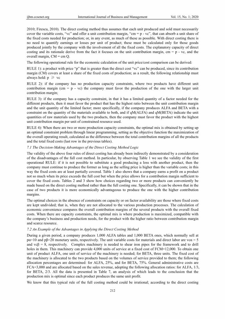
2010; Firescu, 2010). The direct costing method thus assumes that each unit produced and sold must necessarily cover the variable costs, “vc” and offer a unit contribution margin, “cm = p - vc”, that can absorb a unit share of the fixed costs needed for production; or, in any event, as much of these as possible. With direct costing there is no need to quantify earnings or losses per unit of product; these must be calculated only for those goods produced jointly by the company with the involvement of all the fixed costs. The explanatory capacity of direct costing and its rationale derive from the fact it focuses on the unit contribution margin, cm = p - vc, and the overall margin, CM = cm Q. The following operational rule for the economic calculation of the unit price/cost comparison can be derived: RULE 1): a product with price “p” that is greater than the direct cost “vc” can be produced, since its contribution margin (CM) covers at least a share of the fixed costs of production; as a result, the following relationship must always hold: p ≥ vc RULE 2): if the company has no production capacity constraints, where two products have different unit contribution margin (cm = p - vc) the company must favor the production of the one with the larger unit contribution margin; RULE 3): if the company has a capacity constraint, in that it has a limited quantity of a factor needed for the different products, then it must favor the product that has the highest ratio between the unit contribution margin and the unit quantity of the limited factor; more specifically, if the company produces ALFA and BETA with a constraint on the quantity of the materials available to both, and if qM(ALFA) and qM(BETA) indicate the unit quantities of raw materials used by the two products, then the company must favor the product with the highest unit contribution margin per unit of constrained resource used. RULE 4): When there are two or more production capacity constraints, the optimal mix is obtained by setting up an optimal constraint problem through linear programming, setting as the objective function the maximization of the overall operating result, calculated as the difference between the total contribution margins of all the products and the total fixed costs (last row in the previous tables). 7.1 The Decision-Making Advantages of the Direct Costing Method Logic The validity of the above four rules of direct costing has already been indirectly demonstrated by a consideration of the disadvantages of the full cost method. In particular, by observing Table 1 we see the validity of the first operational RULE: if it is not possible to substitute a good producing a loss with another product, then the company must continue to produce the former as long as the selling price is higher than the variable costs; in this way the fixed costs are at least partially covered. Table 1 also shows that a company earns a profit on a product not so much when its price exceeds the full cost but when the price allows for a contribution margin sufficient to cover the fixed costs. Tables 2 and 3 show how choices regarding two or more products can conveniently be made based on the direct costing method rather than the full costing one. Specifically, it can be shown that in the case of two products it is more economically advantageous to produce the one with the higher contribution margins. The optimal choices in the absence of constraints on capacity or on factor availability are those where fixed costs are kept undivided; that is, when they are not allocated to the various production processes. The calculation of economic convenience compares the overall contribution margins of the several products with the overall fixed costs. When there are capacity constraints, the optimal mix is where production is maximized, compatible with the company’s business and production needs, for the product with the higher ratio between contribution margin and scarce resource. 7.2 An Example of the Advantages in Applying the Direct Costing Method During a given period, a company produces 1,000 ALFA tables and 1,000 BETA ones, which normally sell at pα=10 and pβ=20 monetary units, respectively. The unit variable costs for materials and direct labor are vcα = 5 and vcβ = 8, respectively. Complex machinery is needed to shear iron pipes for the framework and to drill holes in them. This machinery can provide 4,000 units of service at a fixed cost of FCM=12,000. To obtain one unit of product ALFA, one unit of service of the machinery is needed; for BETA, three units. The fixed cost of the machinery is allocated to the two products based on the volumes of service provided to them; the following allocation percentages are determined: for ALFA, 25%, and for BETA, 75%. General administrative costs are FCA=3,000 and are allocated based on the sales revenue, adopting the following allocation ratios: for ALFA, 1/3, for BETA, 2/3. All the data is presented in Table 7, an analysis of which leads to the conclusion that the production mix is optimal since each product produces the same unit profit. We know that this typical rule of the full costing method could be irrational; according to the direct costing


213

method, the parameter to observe is the contribution margin. BETA has a higher unit contribution margin, and thus a case can be made to modify the product mix to increase production of BETA. However, the data reveals that production is at full capacity, and thus any change in the production of BETA must be accompanied by a variation in the opposite direction in ALFA production. It must now be decided if it is advantageous to increase the production of BETA while at the same time reducing that of ALFA. Since the capacity constraint concerns units of service of the available machinery, an increase of one unit for BETA, which requires 3 units of service, means reducing ALFA production by 3 units, each of which in turn requires one unit of machine service. Table 7. The full costing and direct costing methods in the case of two products

ALFA Production

BETA Production

Totals

Q = Quantity sold p = Unit price TR = Total Revenues vc = Unit Variable Cost direct cost for materials direct cost for labor VC = Total Variable Cost cm = unit contribution margin = p - cv CM = Contribution Margin Fixed Costs - Machinery Machinery allocation coefficient Fixed Costs - Administrative costs Machinery allocation coefficient FC = Fixed Costs Full Cost = VC + FC fc = unit full cost ur = unit result = p – fc R = Operating Income

1,00010.00

10,0005.002.003.00

5,0005.00

5,0003,00025 %1,000

33.33 %4,0009,000

9.001.00

1,000

1,000 20.00

20,000 8.00 4.00 4.00

8,000 12.00

12,000 9,000 75 % 2,000

66.67 % 11,000 19.000

19.00 1.00

1,000

30,0000

13,000

17,00012,000100 %3,000

100 %15,00028,000

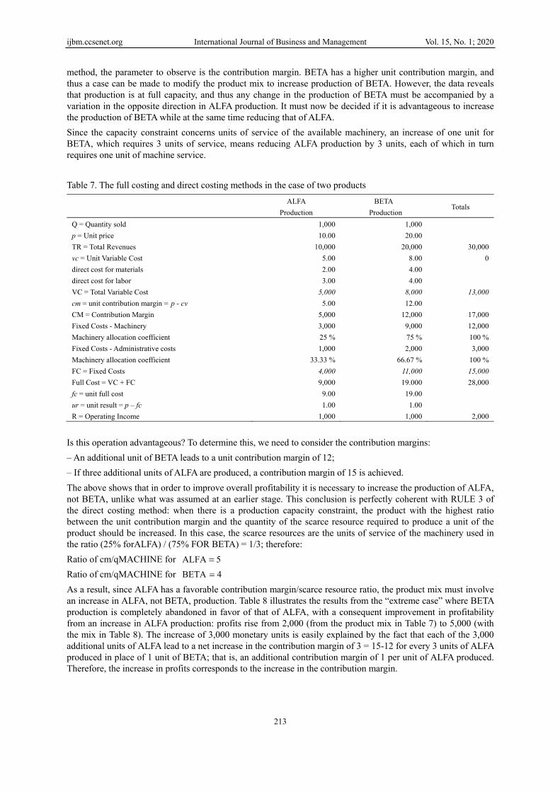
2,000 Is this operation advantageous? To determine this, we need to consider the contribution margins: – An additional unit of BETA leads to a unit contribution margin of 12; – If three additional units of ALFA are produced, a contribution margin of 15 is achieved. The above shows that in order to improve overall profitability it is necessary to increase the production of ALFA, not BETA, unlike what was assumed at an earlier stage. This conclusion is perfectly coherent with RULE 3 of the direct costing method: when there is a production capacity constraint, the product with the highest ratio between the unit contribution margin and the quantity of the scarce resource required to produce a unit of the product should be increased. In this case, the scarce resources are the units of service of the machinery used in the ratio (25% forALFA) / (75% FOR BETA) = 1/3; therefore: Ratio of cm/qMACHINE for 5ALFA = Ratio of cm/qMACHINE for 4BETA = As a result, since ALFA has a favorable contribution margin/scarce resource ratio, the product mix must involve an increase in ALFA, not BETA, production. Table 8 illustrates the results from the “extreme case” where BETA production is completely abandoned in favor of that of ALFA, with a consequent improvement in profitability from an increase in ALFA production: profits rise from 2,000 (from the product mix in Table 7) to 5,000 (with the mix in Table 8). The increase of 3,000 monetary units is easily explained by the fact that each of the 3,000 additional units of ALFA lead to a net increase in the contribution margin of 3 = 15-12 for every 3 units of ALFA produced in place of 1 unit of BETA; that is, an additional contribution margin of 1 per unit of ALFA produced. Therefore, the increase in profits corresponds to the increase in the contribution margin.


214

Table 8. Variation of the product mix in the case of a scarce factor ALFA

Production BETA

Production is interrupted Totals

Q = Quantity sold p = Unit price TR = Total Revenues vc = Unit Variable Cost direct cost for materials direct cost for labor VC = Total Variable Cost cm = unit contribution margin = p - cv CM = Contribution Margin Fixed Costs - Machinery Machinery allocation coefficient Fixed Costs - Administrative costs Machinery allocation coefficient FC = Fixed Costs Full Cost = VC + FC fc = unit full cost ur = unit result = p – fc R = Operating Income

4,00010.00

40,0005.002.003.00

20,0005.00

20,00012,000100 %3,000

100 %15,00035,000

8.751.25

5,000

0 20.00

0 8.00 4.00 4.00

0 12.00

0 0

0 % 0

0 % 0 0

0

40,0000

20,000

20,00012,000100 %3,000

100 %15,00035,000

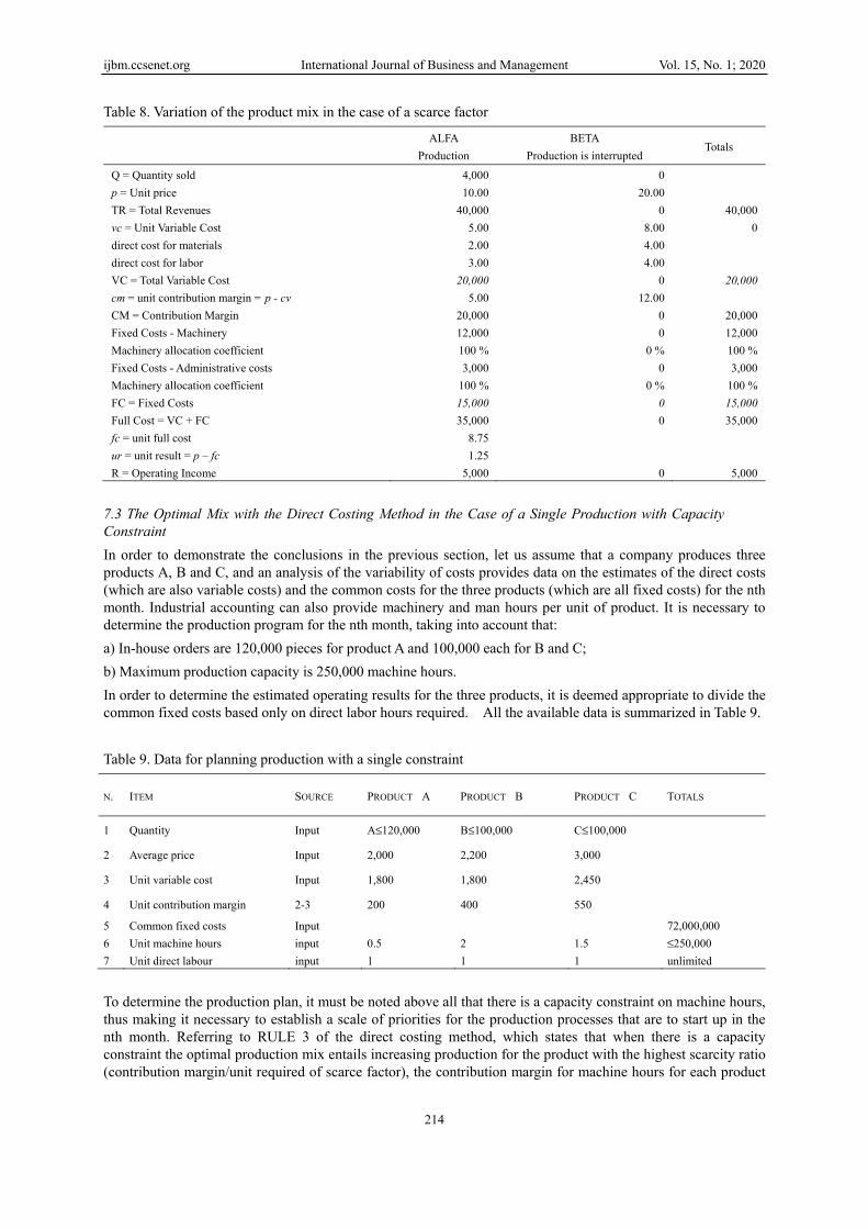
5,000 7.3 The Optimal Mix with the Direct Costing Method in the Case of a Single Production with Capacity Constraint In order to demonstrate the conclusions in the previous section, let us assume that a company produces three products A, B and C, and an analysis of the variability of costs provides data on the estimates of the direct costs (which are also variable costs) and the common costs for the three products (which are all fixed costs) for the nth month. Industrial accounting can also provide machinery and man hours per unit of product. It is necessary to determine the production program for the nth month, taking into account that: a) In-house orders are 120,000 pieces for product A and 100,000 each for B and C; b) Maximum production capacity is 250,000 machine hours. In order to determine the estimated operating results for the three products, it is deemed appropriate to divide the common fixed costs based only on direct labor hours required. All the available data is summarized in Table 9. Table 9. Data for planning production with a single constraint

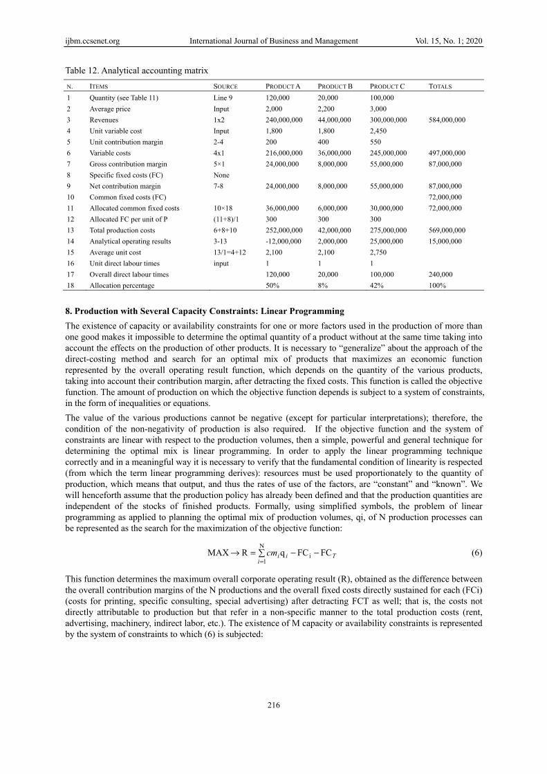
N. ITEM SOURCE PRODUCT A PRODUCT B PRODUCT C TOTALS

1 Quantity Input A≤120,000 B≤100,000 C≤100,000

2 Average price Input 2,000 2,200 3,000

3 Unit variable cost Input 1,800 1,800 2,450

4 Unit contribution margin 2-3 200 400 550

5 Common fixed costs Input 72,000,000 6 Unit machine hours input 0.5 2 1.5 ≤250,000 7 Unit direct labour input 1 1 1 unlimited To determine the production plan, it must be noted above all that there is a capacity constraint on machine hours, thus making it necessary to establish a scale of priorities for the production processes that are to start up in the nth month. Referring to RULE 3 of the direct costing method, which states that when there is a capacity constraint the optimal production mix entails increasing production for the product with the highest scarcity ratio (contribution margin/unit required of scarce factor), the contribution margin for machine hours for each product


215

must first be determined, as indicated in Table 10. Table 10. Order of preference based on the scarcity ratio N. ITEM SOURCE PRODUCT A PRODUCT B PRODUCT C TOTALS

1 Quantity Input A≤120,000 B≤100,000 C≤100,000

2 Average price Input 2,000 2,200 3,000

3 Unit variable cost input 1,800 1,800 2,450

4 Unit contribution margin 2-3 200 400 550

5 Unit machine times input 0.5 2 1.5 ≤250,000

6 Scarcity ratio 4/5 400 200 367

7 ORDER OF PREFERENCE I III II

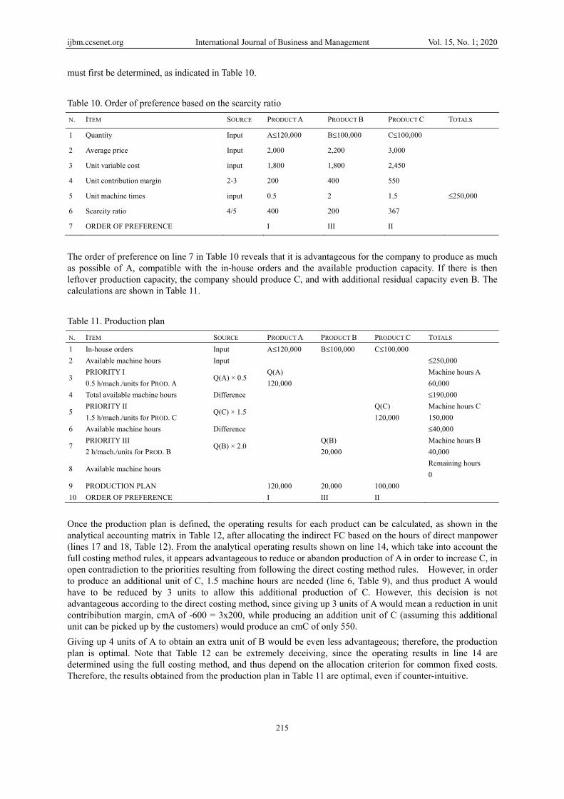
The order of preference on line 7 in Table 10 reveals that it is advantageous for the company to produce as much as possible of A, compatible with the in-house orders and the available production capacity. If there is then leftover production capacity, the company should produce C, and with additional residual capacity even B. The calculations are shown in Table 11. Table 11. Production plan N. ITEM SOURCE PRODUCT A PRODUCT B PRODUCT C TOTALS 1 In-house orders Input A≤120,000 B≤100,000 C≤100,000 2 Available machine hours Input ≤250,000

3 PRIORITY I 0.5 h/mach./units for PROD. A

Q(A) × 0.5 Q(A) 120,000

Machine hours A 60,000

4 Total available machine hours Difference ≤190,000

5 PRIORITY II 1.5 h/mach./units for PROD. C

Q(C) × 1.5 Q(C) 120,000

Machine hours C 150,000

6 Available machine hours Difference ≤40,000

7 PRIORITY III 2 h/mach./units for PROD. B

Q(B) × 2.0 Q(B) 20,000

Machine hours B 40,000

8 Available machine hours Remaining hours 0

9 PRODUCTION PLAN 120,000 20,000 100,000 10 ORDER OF PREFERENCE I III II Once the production plan is defined, the operating results for each product can be calculated, as shown in the analytical accounting matrix in Table 12, after allocating the indirect FC based on the hours of direct manpower (lines 17 and 18, Table 12). From the analytical operating results shown on line 14, which take into account the full costing method rules, it appears advantageous to reduce or abandon production of A in order to increase C, in open contradiction to the priorities resulting from following the direct costing method rules. However, in order to produce an additional unit of C, 1.5 machine hours are needed (line 6, Table 9), and thus product A would have to be reduced by 3 units to allow this additional production of C. However, this decision is not advantageous according to the direct costing method, since giving up 3 units of A would mean a reduction in unit contribibution margin, cmA of -600 = 3x200, while producing an addition unit of C (assuming this additional unit can be picked up by the customers) would produce an cmC of only 550. Giving up 4 units of A to obtain an extra unit of B would be even less advantageous; therefore, the production plan is optimal. Note that Table 12 can be extremely deceiving, since the operating results in line 14 are determined using the full costing method, and thus depend on the allocation criterion for common fixed costs. Therefore, the results obtained from the production plan in Table 11 are optimal, even if counter-intuitive.


216

Table 12. Analytical accounting matrix N. ITEMS SOURCE PRODUCT A PRODUCT B PRODUCT C TOTALS 1 Quantity (see Table 11) Line 9 120,000 20,000 100,000 2 Average price Input 2,000 2,200 3,000 3 Revenues 1x2 240,000,000 44,000,000 300,000,000 584,000,000 4 Unit variable cost Input 1,800 1,800 2,450 5 Unit contribution margin 2-4 200 400 550 6 Variable costs 4x1 216,000,000 36,000,000 245,000,000 497,000,000 7 Gross contribution margin 5×1 24,000,000 8,000,000 55,000,000 87,000,000 8 Specific fixed costs (FC) None 9 Net contribution margin 7-8 24,000,000 8,000,000 55,000,000 87,000,000 10 Common fixed costs (FC) 72,000,000 11 Allocated common fixed costs 10×18 36,000,000 6,000,000 30,000,000 72,000,000 12 Allocated FC per unit of P (11+8)/1 300 300 300 13 Total production costs 6+8+10 252,000,000 42,000,000 275,000,000 569,000,000 14 Analytical operating results 3-13 -12,000,000 2,000,000 25,000,000 15,000,000 15 Average unit cost 13/1=4+12 2,100 2,100 2,750 16 Unit direct labour times input 1 1 1 17 Overall direct labour times 120,000 20,000 100,000 240,000 18 Allocation percentage 50% 8% 42% 100% 8. Production with Several Capacity Constraints: Linear Programming The existence of capacity or availability constraints for one or more factors used in the production of more than one good makes it impossible to determine the optimal quantity of a product without at the same time taking into account the effects on the production of other products. It is necessary to “generalize” about the approach of the direct-costing method and search for an optimal mix of products that maximizes an economic function represented by the overall operating result function, which depends on the quantity of the various products, taking into account their contribution margin, after detracting the fixed costs. This function is called the objective function. The amount of production on which the objective function depends is subject to a system of constraints, in the form of inequalities or equations. The value of the various productions cannot be negative (except for particular interpretations); therefore, the condition of the non-negativity of production is also required. If the objective function and the system of constraints are linear with respect to the production volumes, then a simple, powerful and general technique for determining the optimal mix is linear programming. In order to apply the linear programming technique correctly and in a meaningful way it is necessary to verify that the fundamental condition of linearity is respected (from which the term linear programming derives): resources must be used proportionately to the quantity of production, which means that output, and thus the rates of use of the factors, are “constant” and “known”. We will henceforth assume that the production policy has already been defined and that the production quantities are independent of the stocks of finished products. Formally, using simplified symbols, the problem of linear programming as applied to planning the optimal mix of production volumes, qi, of N production processes can be represented as the search for the maximization of the objective function:

Ti

iicm FCFCqR MAX iN

1−−=→

= (6)

This function determines the maximum overall corporate operating result (R), obtained as the difference between the overall contribution margins of the N productions and the overall fixed costs directly sustained for each (FCi) (costs for printing, specific consulting, special advertising) after detracting FCT as well; that is, the costs not directly attributable to production but that refer in a non-specific manner to the total production costs (rent, advertising, machinery, indirect labor, etc.). The existence of M capacity or availability constraints is represented by the system of constraints to which (6) is subjected:


217

≤

≤

≤

=

=

=

N

1MM

N

122

N

111

bqc

...

bqc

bqc

iii

iii

iii

(7)

where the coefficients cji represent the unit consumption of the jth limited factor for the ith production process. Finally, the conditions of non-negativity must hold:

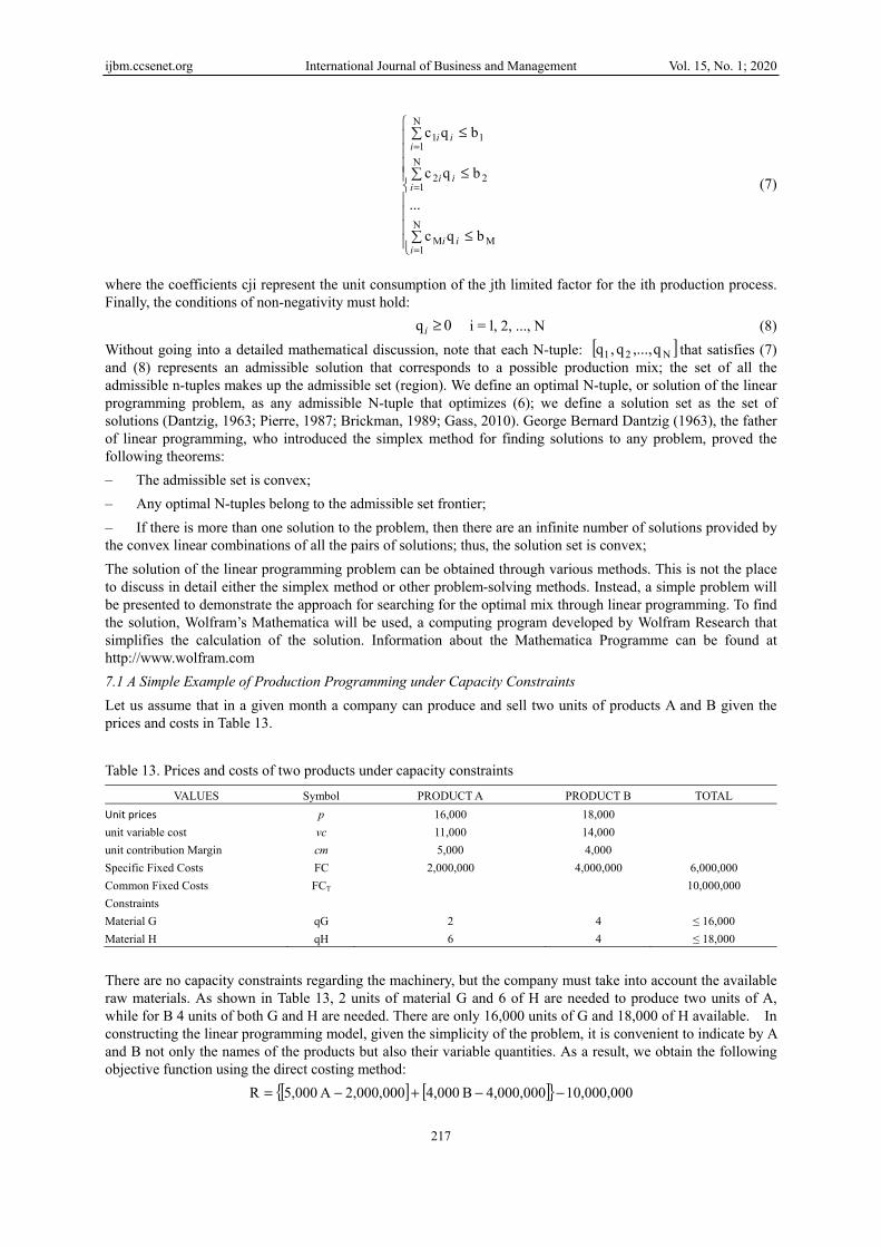
0q ≥i i = l, 2, ..., N (8) Without going into a detailed mathematical discussion, note that each N-tuple: [ ]N21 q,...,q,q that satisfies (7) and (8) represents an admissible solution that corresponds to a possible production mix; the set of all the admissible n-tuples makes up the admissible set (region). We define an optimal N-tuple, or solution of the linear programming problem, as any admissible N-tuple that optimizes (6); we define a solution set as the set of solutions (Dantzig, 1963; Pierre, 1987; Brickman, 1989; Gass, 2010). George Bernard Dantzig (1963), the father of linear programming, who introduced the simplex method for finding solutions to any problem, proved the following theorems: – The admissible set is convex; – Any optimal N-tuples belong to the admissible set frontier; – If there is more than one solution to the problem, then there are an infinite number of solutions provided by the convex linear combinations of all the pairs of solutions; thus, the solution set is convex; The solution of the linear programming problem can be obtained through various methods. This is not the place to discuss in detail either the simplex method or other problem-solving methods. Instead, a simple problem will be presented to demonstrate the approach for searching for the optimal mix through linear programming. To find the solution, Wolfram’s Mathematica will be used, a computing program developed by Wolfram Research that simplifies the calculation of the solution. Information about the Mathematica Programme can be found at http://www.wolfram.com 7.1 A Simple Example of Production Programming under Capacity Constraints Let us assume that in a given month a company can produce and sell two units of products A and B given the prices and costs in Table 13. Table 13. Prices and costs of two products under capacity constraints

VALUES Symbol PRODUCT A PRODUCT B TOTAL Unit prices p 16,000 18,000 unit variable cost vc 11,000 14,000 unit contribution Margin cm 5,000 4,000 Specific Fixed Costs FC 2,000,000 4,000,000 6,000,000 Common Fixed Costs FCT 10,000,000 Constraints Material G qG 2 4 ≤ 16,000 Material H qH 6 4 ≤ 18,000 There are no capacity constraints regarding the machinery, but the company must take into account the available raw materials. As shown in Table 13, 2 units of material G and 6 of H are needed to produce two units of A, while for B 4 units of both G and H are needed. There are only 16,000 units of G and 18,000 of H available. In constructing the linear programming model, given the simplicity of the problem, it is convenient to indicate by A and B not only the names of the products but also their variable quantities. As a result, we obtain the following objective function using the direct costing method:

[ ] [ ]{ } 10,000,0004,000,000B 4,0002,000,000A 5,000R −−+−=


218

[ ] B. 4,000A 5,00016,000,000R +=+

[ ]1,000

16,000,000RZ +=

Simplifying the above, the objective function is thus simply (ignoring for the moment the constant amount of units of material, 16,000):

B 4A 5 Zmax +=

Table 13 easily provides us with the system of constraints:

.negativity-non ofcondition 0 ≥ B A,H material of constraint 18,000 ≤ B 4+A 6G material of constraint 16,000 ≤ B 4+A 2

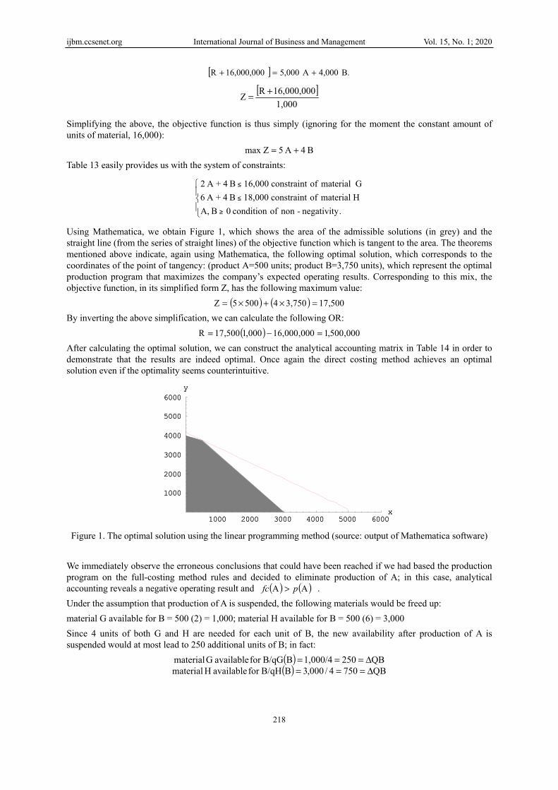
Using Mathematica, we obtain Figure 1, which shows the area of the admissible solutions (in grey) and the straight line (from the series of straight lines) of the objective function which is tangent to the area. The theorems mentioned above indicate, again using Mathematica, the following optimal solution, which corresponds to the coordinates of the point of tangency: (product A=500 units; product B=3,750 units), which represent the optimal production program that maximizes the company’s expected operating results. Corresponding to this mix, the objective function, in its simplified form Z, has the following maximum value:

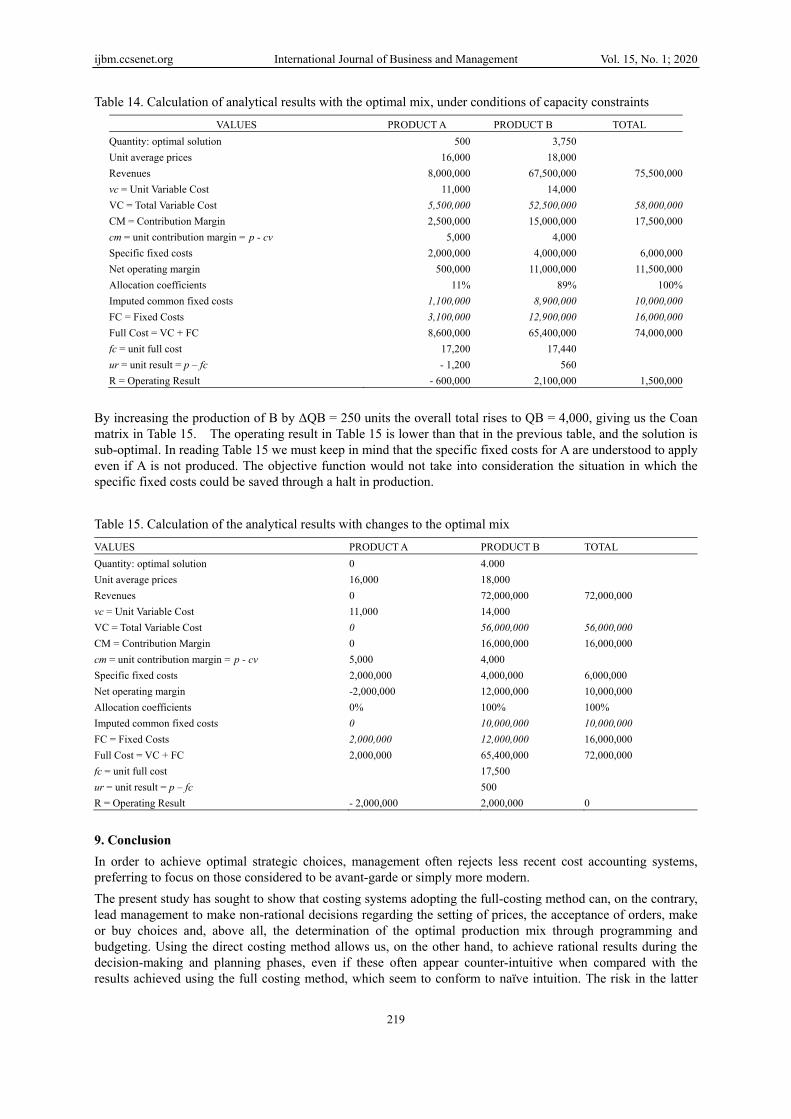
( ) ( ) 500,173,7504 5005Z =×+×= By inverting the above simplification, we can calculate the following OR:

( ) 000,500,1000,000,16000,1500,17R =−= After calculating the optimal solution, we can construct the analytical accounting matrix in Table 14 in order to demonstrate that the results are indeed optimal. Once again the direct costing method achieves an optimal solution even if the optimality seems counterintuitive.

Figure 1. The optimal solution using the linear programming method (source: output of Mathematica software) We immediately observe the erroneous conclusions that could have been reached if we had based the production program on the full-costing method rules and decided to eliminate production of A; in this case, analytical accounting reveals a negative operating result and ( ) ( )AA pfc > . Under the assumption that production of A is suspended, the following materials would be freed up: material G available for B = 500 (2) = 1,000; material H available for B = 500 (6) = 3,000 Since 4 units of both G and H are needed for each unit of B, the new availability after production of A is suspended would at most lead to 250 additional units of B; in fact:

( ) QB2501,000/4BB/qGfor availableG material Δ===( ) QB7504/000,3BB/qHfor available H material Δ===

1000 2000 3000 4000 5000 6000x

1000

2000

3000

4000

5000

6000y

1000 2000 3000 4000 5000 6000x

1000

2000

3000

4000

5000

6000y


219

Table 14. Calculation of analytical results with the optimal mix, under conditions of capacity constraints VALUES PRODUCT A PRODUCT B TOTAL

Quantity: optimal solution 500 3,750Unit average prices 16,000 18,000Revenues 8,000,000 67,500,000 75,500,000vc = Unit Variable Cost 11,000 14,000VC = Total Variable Cost 5,500,000 52,500,000 58,000,000CM = Contribution Margin 2,500,000 15,000,000 17,500,000cm = unit contribution margin = p - cv 5,000 4,000Specific fixed costs 2,000,000 4,000,000 6,000,000Net operating margin 500,000 11,000,000 11,500,000Allocation coefficients 11% 89% 100%Imputed common fixed costs 1,100,000 8,900,000 10,000,000FC = Fixed Costs 3,100,000 12,900,000 16,000,000Full Cost = VC + FC 8,600,000 65,400,000 74,000,000fc = unit full cost 17,200 17,440ur = unit result = p – fc - 1,200 560R = Operating Result - 600,000 2,100,000 1,500,000

By increasing the production of B by ΔQB = 250 units the overall total rises to QB = 4,000, giving us the Coan matrix in Table 15. The operating result in Table 15 is lower than that in the previous table, and the solution is sub-optimal. In reading Table 15 we must keep in mind that the specific fixed costs for A are understood to apply even if A is not produced. The objective function would not take into consideration the situation in which the specific fixed costs could be saved through a halt in production. Table 15. Calculation of the analytical results with changes to the optimal mix VALUES PRODUCT A PRODUCT B TOTAL Quantity: optimal solution 0 4.000 Unit average prices 16,000 18,000 Revenues 0 72,000,000 72,000,000 vc = Unit Variable Cost 11,000 14,000 VC = Total Variable Cost 0 56,000,000 56,000,000 CM = Contribution Margin 0 16,000,000 16,000,000 cm = unit contribution margin = p - cv 5,000 4,000 Specific fixed costs 2,000,000 4,000,000 6,000,000 Net operating margin -2,000,000 12,000,000 10,000,000 Allocation coefficients 0% 100% 100% Imputed common fixed costs 0 10,000,000 10,000,000 FC = Fixed Costs 2,000,000 12,000,000 16,000,000 Full Cost = VC + FC 2,000,000 65,400,000 72,000,000 fc = unit full cost 17,500 ur = unit result = p – fc 500 R = Operating Result - 2,000,000 2,000,000 0 9. Conclusion In order to achieve optimal strategic choices, management often rejects less recent cost accounting systems, preferring to focus on those considered to be avant-garde or simply more modern. The present study has sought to show that costing systems adopting the full-costing method can, on the contrary, lead management to make non-rational decisions regarding the setting of prices, the acceptance of orders, make or buy choices and, above all, the determination of the optimal production mix through programming and budgeting. Using the direct costing method allows us, on the other hand, to achieve rational results during the decision-making and planning phases, even if these often appear counter-intuitive when compared with the results achieved using the full costing method, which seem to conform to naïve intuition. The risk in the latter


220

case is even more serious when we are dealing with multi-production firms operating under conditions of limited production capacity regarding one or more factors, as occurs most of the time. Though simplified, the numerical examples presented above provide ample proof of the superiority of direct costing with respect to full costing, above all for the following important managerial decisions: – How to set profitable prices on the basis of the unit cost data and, vice-versa, which target costs must be achieed taking into account the predetermined prices; – Whether or not to activate or de-activate a production process, given the estimated selling prices; – Which product mix is most rational given the selling prices and unit costs of production, especially in the case of multiple constraints. This study does not intend to provide analytical solutions to the problems at hand, since this was not its original objective. Nevertheless, the hope is that it has aroused the “suspicion” that several modern costing systems, based on the full costing method, “are not infallible”, and that when using cost data for business decisions and budget preparation some “reflection” on the dynamics of costs in relation to production volumes is necessary. References Ansari, S. L., & Bell, J. E. (1997). Target Costing: The Next Frontier in Strategic Cost Management: The CAM-1

Target Cost Core Group. Chicago: Irwin Professional Publishing. Avi, M. S. (2012). Management Accounting. Cost Analysis, EIF ebook. Baxendale, S. J., & Foster, B. P. (2010). ABC absorption and direct costing income statements. Cost

Management, 24(5), 5-14. Bebbington, J., & Gray, R. (2001). An account of sustainability: failure, success and a reconceptualization.

Critical perspectives on accounting, 12(5), 557-587. https://doi.org/10.1006/cpac.2000.0450 Bhimani, A., & Pigott, D. (1992). Implementing ABC: A case study of organizational and behavioural

consequences. Management Accounting Research, 3(2), 119-132. https://doi.org/10.1016/S1044-5005(92)70007-9

Brickman, L. (2012). Mathematical introduction to linear programming and game theory. Undergraduate Texts in Mathematics). Springer Science and Business Media.

Brimson, J. A. (2007). An ABC retrospective:" mirror, mirror on the wall...". Journal of cost management, 21(2), 45-47.

Cafferky, M. (2010). Breakeven Analysis: The Definitive Guide to Cost-Volume-Profit Analysis. Managerial Accounting Collection: Business Expert Press. https://doi.org/10.4128/9781606490174

Cooper, R. (1988a). ABC: key to future costs. Management Consultancy, 10, 1-3. Cooper, R. (1988b). The rise of activity based costing – Part one: What is an activity based cost system? Journal

of Cost Management, 41-48. Cooper, R. (1989). The rise of activity based costing – Part three: How many cost drivers do you need and how

do you select them? Journal of Cost Management, 34-46. Cooper, R., & Chew, W. B. (1996). Control tomorrow's costs through today's designs. Harvard Business Review,

74(1), 88-97. Cooper, R., & Kaplan, R. S. (1988a). Measure costs right: make the right decisions. Harvard Business Review,

66(5), 96-103. Cooper, R., & Kaplan, R. S. (1988b). How cost accounting distorts product costs. Strategic Finance, 69(10),

20-27. Cooper, R., & Kaplan, R. S. (1991). Profit priorities from activity-based costing. Harvard Business Review,

69(3), 130-135. Dantzig, G. B. (1963). Linear programming and extensions. Princeton, NJ: Princeton university Press.

https://doi.org/10.7249/R366 Drury, C. M. (2013). Management and cost accounting. New York, NY, Dordrecht, London: Springer. DuBrin, A. J. (2008). Essentials of Management. Mason: South-Western, Cengage Learning. Dugdale, D., & Jones, T. C. (1997). How many companies use ABC for stock valuation ? A comment on Innes


221

and Mitchell's questionnaire findings. Management Accounting Research, 8(2), 233-240. https://doi.org/10.1006/mare.1996.0043

Fess, P. E., & Ferrara, W. L. (1961). The period cost concept for income measurement-can it be defended? The Accounting Review, 36(4), 598-611.

Firescu, V. (2010). The importance of the calculation methods based on direct costing in managerial decisions. Scientific Bulletin-Economic Sciences, 9(15), 75-82

Fremgen, J. M. (1964). The Direct costing controversy-An identification of issues. The Accounting Review, 39(1), 43-53.

Gass, I. S. (2010). Linear Programming: Methods and Applications (5th ed.). Dover: Dover Publications Gramlich, J. P., & Korok, R. (2015). Reconciling Full-Cost and Marginal-Cost Pricing, Finance and Economics

Discussion Series 2015-072. Washington: Board of Governors of the Federal Reserve System. Guerreiro, R., Bio, S. R., & Casado, T. (2004). Some reflections on the archetypes in cost accounting: an

exploratory study. Journal of Applied Management Accounting Research, 2(1), 41-48. https://doi.org/10.17016/FEDS.2015.072

Hansen, S. C., & Van der Stede, W. A. (2004). Multiple facets of budgeting: an exploratory analysis. Management accounting research, 15(4), 415-439. https://doi.org/10.1016/j.mar.2004.08.001

Homburg, C. (2001). A note on optimal cost driver selection in ABC. Management Accounting Research, 12(2), 197-205. https://doi.org/10.1006/mare.2000.0150

Horngren, C. T. (1972). Cost Accounting: A Managerial Emphasis. Inc. Englewood Cliffs, New Jersey: Prentice-Hall.

Horngren, C. T., & Sorter, G. H. (1961). "Direct" Costing for External Reporting. The Accounting Review, 36(1), 84-89.

Jasinski, D., Meredith, J., & Kirwan, K. (2015). A comprehensive review of full cost accounting methods and their applicability to the automotive industry. Journal of Cleaner Production, 108, 1123-1139. https://doi.org/10.1016/j.jclepro.2015.06.040

Johnson, H., & Kaplan, R. (1987). Relevance Lost – The Rise and Fall of Management Accounting. Boston, MA: Harvard Business School Press.

Kaplan, R. (1984). The Evolution of Management Accounting. The Accounting Review, 59(3), 390-418. Kaplan, R. S., & Johnson, H. T. (1987). Relevance lost. The rise and fall of management accounting. Boston,

Mass: Harvard Business School Press. Kato, Y. (1993), Target costing support systems: lessons from leading Japanese companies. Management

Accounting Research, 4(1), 33-47. https://doi.org/10.1006/mare.1993.1002 Krishnan, S., & Lin, P. (2012), Inventory Valuation Under IFRS and GAAP. Strategic finance, 93(9), 51-59. Mac Arthur, J. B. (1993). Theory of Constraint and activity based costing: friends or foes? Journal of Cost

Management, 7(2), 50-56. McIntyre, E. V. (1999). Accounting choices and EVA. Business Horizons, 42(1), 66-73.

https://doi.org/10.1016/S0007-6813(99)80050-0 Mella P. (1997). Management control (original: Controllo di gestione). Torino, IT: Utet. Mella, P. (2005). Performance Indicators in Business Value-Creating Organizations. Economia Aziendale 2000

Web, 2(2), 25- 52. Mella, P. (2012). Systems Thinking. Intelligence in Action. New York, NY, Dordrecht, London: Springer.

https://doi.org/10.1007/978-88-470-2565-3 Mella, P. (2014). The Magic Ring. Systems thinking Approach to Control Systems. New York, NY, Dordrecht,

London: Springer. https://doi.org/10.1007/978-3-319-05386-8 Mella, P. (2018a). Quality a Key Value Driver in Value Based Management. Economia Aziendale Online, 9(4),

439-462. https://doi.org/10.13132/2038-5498/9.4.1970 Mella, P. (2018b). The law of increasing productivity. Int. J. Markets and Business Systems, 3(4), 297-316.

https://doi.org/10.1504/IJMABS.2018.097899


222

Mitchell, F. (1994). A commentary on the applications of activity-based costing, Management Accounting Research, 5(3-4), 261-277. https://doi.org/10.1006/mare.1994.1016

Moisello, A. M. (2012a), Costing for Decision Making: Activity-based Costing vs. Theory of Constraints. International Journal of Knowledge, Culture and Change in Organizations: Annual Review, 12(1), 1-13. https://doi.org/10.18848/1447-9524/CGP/v12/50968

Moisello, A. M. (2012b). Cost measurement and cost management in target costing. The Annals of the University of Oradea, 1(1), 533-547.

Moisello, A. (2012c). ABC & EVA: un’integrazione possibile –La valutazione del costo di prodotto nell’ottica della creazione di valore. Economia Aziendale Online, (1), 25-40.

Moisello, A. M. (2000). Production costs (original: I costi di produzione). Milano, IT: Egea. Moss, M. F., & Haseman, W. C. (1957). Some Comments on the Applicability of Direct Costing to Decision

Making. The Accounting Review, 32(2), 184-193. Moyer, C. R., McGuigan, J. R., & Rao, R. P. (2014). Contemporary Financial Management. Cengage Learning. Noreen, E., Smith, D., & Mackey, J. T. (1995). Theory of constraints and its implications for management

accounting: A report on the actual implementation of the theory of constraints. Great Barrington, MA: North River Press, Incorporated.

Ogungbade, O. I., & Tabitha, N. (2018). Cost Accounting Techniques Adopted by Manufacturing and Service Industry within the Last Decade. International Journal of Advances in Management and Economics, 5(1), 48-61.

Paton, W. A., & Littleton, A. C. (1940). An Introduction to Corporate Accounting Standards. Monograph No. 3. Chicago, IL: American Accounting Association.

Pierre, D. A. (1987). Optimization Theory with Applications. New York, NY: Dover Publications. Pong, C., & Mitchell, F. (2006). Full costing versus variable costing: Does the choice still matter? An empirical

exploration of UK manufacturing companies 1988–2002. The British Accounting Review, 38(2), 131-148. https://doi.org/10.1016/j.bar.2005.09.003

Rajasekaran, V., & Lalitha, R. (2011). Cost Accounting. Dorling Kindersley, New Delhi, IN: Pearson. Sponem, S., & Lambert, C. (2016), Exploring differences in budget characteristics, roles and satisfaction: A

configurational approach. Management Accounting Research, 30, 47-61. https://doi.org/10.1016/j.mar.2015.11.003

Staubus, G. J. (1963). Direct, Relevant or Absorption Costing. The Accounting Review, 38(1), 64. Waweru, N.M. (2010). The origin and evolution of management accounting: A review of the theoretical

framework. Problems and Perspectives in Management, 8(3), 165-182. Copyrights Copyright for this article is retained by the author(s), with first publication rights granted to the journal. This is an open-access article distributed under the terms and conditions of the Creative Commons Attribution license (http://creativecommons.org/licenses/by/4.0/).

Documents

Matching Revenues and Costs: The Counter-Intuitive