Match-Making in Bartering Scenarios

by

Sebastien Mathieu

A Thesis Submitted in Partial Fulfilment ofthe Requirements for the Degree of

Master of Computer Science

in the Graduate Academic Unit of Computer Science

Supervisors: Dr. Virendra C. Bhavsar, PhD (IIT/Bombay), Computer ScienceDr. Harold Boley, Ph.D (Hamburg), Computer Science

Examining Board: Prof. John DeDourek, MS (Case Western), Computer Science,ChairDr. Weichang Du, PhD (U of Vic), Computer ScienceDr. Donglei Du, PhD (Dallas), Business Administration

This thesis is accepted by theDean of Graduate Studies

THE UNIVERSITY OF NEW BRUNSWICK

December, 2005

c©Sebastien Mathieu, 2006

Abstract

This thesis extends tree similarity based match-making from the buyer/seller situa-

tion to a scenario of bilateral bartering and multi-agent ring bartering. It is built

on top of the AgentMatcher tree similarity algorithm for node-labelled, arc-labelled,

arc-weighted trees. A representation of these trees in a multi-dimensional space is

developed to allow efficient indexing and pruning in large tree databases. The con-

cept of risk is introduced to control the process of bartering ring construction. We

have tested our system on the Teclantic.ca portal, where it allows researchers and

companies from Atlantic Canada to share technologies as well as to be contacted by

investors.

ii

Acknowledgements

First and foremost, I would like to express my appreciation to my supervisors, Dr.

Virendra C. Bhavsar and Dr. Harold Boley, who gave me a great deal of support

throughout my time at UNB. They continuously contributed their time, effort and

thought in guiding and helping me during the research and writing of this thesis.

Also, I am grateful to the Faculty of Computer Science for their support, and

to my thesis committee members. Special thanks go to Ms. Linda Sales and all her

administrative colleagues for their direction and help, and to all system support staff

for their technical assistance.

I also thank the AgentMatcher research group for their support and advice.

In particular, I also thank Mr. Lu Yang and Mr. Marcel Ball whose work predates

my own, and who helped me understanding their accomplishments.

Finally, I am grateful to all other people in the Faculty of Computer Science who

have assisted me in the course of this work.

iii

Table of Contents

Abstract . . . . . . . . . . . . . . . . . . . . . . . . . . . . . . . . . . . . . . ii

Acknowledgements . . . . . . . . . . . . . . . . . . . . . . . . . . . . . . . iii

List of Figures . . . . . . . . . . . . . . . . . . . . . . . . . . . . . . . . . . ix

List of Tables . . . . . . . . . . . . . . . . . . . . . . . . . . . . . . . . . . . xi

Glossary . . . . . . . . . . . . . . . . . . . . . . . . . . . . . . . . . . . . . . xii

1 Introduction . . . . . . . . . . . . . . . . . . . . . . . . . . . . . . . . . . 1

1.1 eCommerce . . . . . . . . . . . . . . . . . . . . . . . . . . . . . . . . 1

1.1.1 Web portals . . . . . . . . . . . . . . . . . . . . . . . . . . . . 2

1.1.2 Match-Making . . . . . . . . . . . . . . . . . . . . . . . . . . . 2

1.1.3 Bartering . . . . . . . . . . . . . . . . . . . . . . . . . . . . . 3

1.2 Motivation and Approach . . . . . . . . . . . . . . . . . . . . . . . . 4

iv

1.2.1 Representation of Queries . . . . . . . . . . . . . . . . . . . . 4

1.2.2 Match-Making for Bartering Scenarios . . . . . . . . . . . . . 5

1.2.3 Ring Bartering . . . . . . . . . . . . . . . . . . . . . . . . . . 6

1.3 Objectives . . . . . . . . . . . . . . . . . . . . . . . . . . . . . . . . . 6

1.4 Organization of the Thesis . . . . . . . . . . . . . . . . . . . . . . . . 7

2 Match-Making and Bartering . . . . . . . . . . . . . . . . . . . . . . . 8

2.1 Match-Making . . . . . . . . . . . . . . . . . . . . . . . . . . . . . . . 9

2.1.1 Agent-Mediated eCommerce System with Decision Analysis Fea-tures . . . . . . . . . . . . . . . . . . . . . . . . . . . . . . . . 9

2.1.2 The Weighted Tree Similarity Algorithm . . . . . . . . . . . . 10

2.1.2.1 Arc-labelled Weighted Trees for Query Representation 10

2.1.2.2 Description of the Algorithm . . . . . . . . . . . . . 11

2.1.2.3 The AgentMatcher Architecture . . . . . . . . . . . . 12

2.2 Bartering . . . . . . . . . . . . . . . . . . . . . . . . . . . . . . . . . 13

2.2.1 Ring Bartering . . . . . . . . . . . . . . . . . . . . . . . . . . 13

3 Bartering Trees . . . . . . . . . . . . . . . . . . . . . . . . . . . . . . . . 15

3.1 Bartering Trees . . . . . . . . . . . . . . . . . . . . . . . . . . . . . . 15

3.2 Aggregate Similarity . . . . . . . . . . . . . . . . . . . . . . . . . . . 16

3.2.1 Motivation . . . . . . . . . . . . . . . . . . . . . . . . . . . . . 17

3.2.2 Aggregation Function . . . . . . . . . . . . . . . . . . . . . . . 18

3.2.3 Polynomial Approximation . . . . . . . . . . . . . . . . . . . . 22

3.3 Summary and Remarks . . . . . . . . . . . . . . . . . . . . . . . . . . 25

4 Tree Approximation in a Multi-Dimensional Space . . . . . . . . . 26

v

4.1 Motivation . . . . . . . . . . . . . . . . . . . . . . . . . . . . . . . . . 26

4.2 Tree Representation in a Multi-dimensional Space . . . . . . . . . . 28

4.2.1 Definition of the Multi-dimensional Space . . . . . . . . . . . 29

4.2.2 Representation of the Trees . . . . . . . . . . . . . . . . . . . 31

4.2.3 Keeping Information on Nodes and Leaves . . . . . . . . . . . 32

4.3 Notion of Distance . . . . . . . . . . . . . . . . . . . . . . . . . . . . 34

4.3.1 Definition . . . . . . . . . . . . . . . . . . . . . . . . . . . . . 34

4.3.2 Behavior . . . . . . . . . . . . . . . . . . . . . . . . . . . . . . 35

4.4 Order Preserving Linear Hashing . . . . . . . . . . . . . . . . . . . . 36

4.4.1 Principle . . . . . . . . . . . . . . . . . . . . . . . . . . . . . . 36

4.4.2 Range Queries . . . . . . . . . . . . . . . . . . . . . . . . . . . 36

4.5 Remarks . . . . . . . . . . . . . . . . . . . . . . . . . . . . . . . . . . 37

5 Ring Bartering . . . . . . . . . . . . . . . . . . . . . . . . . . . . . . . . 39

5.1 Preliminaries . . . . . . . . . . . . . . . . . . . . . . . . . . . . . . . 39

5.1.1 Definition of a Bartering Ring . . . . . . . . . . . . . . . . . . 40

5.1.2 Generalized Aggregate Similarity . . . . . . . . . . . . . . . . 40

5.2 Notion of Risk . . . . . . . . . . . . . . . . . . . . . . . . . . . . . . . 41

5.2.1 Definition . . . . . . . . . . . . . . . . . . . . . . . . . . . . . 41

5.2.2 Requirement for the Ring Bartering Algorithm . . . . . . . . . 42

5.2.3 Remarks . . . . . . . . . . . . . . . . . . . . . . . . . . . . . . 45

5.2.3.1 Generalized Aggregate Similarity and Risk . . . . . . 45

5.2.3.2 Improvement of the Risk Estimate . . . . . . . . . . 45

5.3 Ring Bartering Algorithm . . . . . . . . . . . . . . . . . . . . . . . . 46

vi

5.3.1 Description of the Algorithm . . . . . . . . . . . . . . . . . . . 46

5.3.2 Details of the Algorithm . . . . . . . . . . . . . . . . . . . . . 46

5.3.2.1 The Selection of Closest Offers . . . . . . . . . . . . 47

5.3.2.2 The Closure of the Ring . . . . . . . . . . . . . . . . 48

5.3.2.3 The Testing of the Risk . . . . . . . . . . . . . . . . 49

5.3.2.4 Overall Algorithm . . . . . . . . . . . . . . . . . . . 51

5.3.3 Properties of the Algorithm . . . . . . . . . . . . . . . . . . . 52

5.4 Extended Algorithm for Bartering Tuples . . . . . . . . . . . . . . . . 54

5.4.1 The Closure of the Ring . . . . . . . . . . . . . . . . . . . . . 54

5.4.2 The Testing of the Risk . . . . . . . . . . . . . . . . . . . . . 55

5.5 Discussion . . . . . . . . . . . . . . . . . . . . . . . . . . . . . . . . . 56

5.5.1 Limitations . . . . . . . . . . . . . . . . . . . . . . . . . . . . 56

5.5.2 Case of Small Databases . . . . . . . . . . . . . . . . . . . . . 56

5.5.3 Storing similarity values . . . . . . . . . . . . . . . . . . . . . 57

5.5.4 Bidirectional Search . . . . . . . . . . . . . . . . . . . . . . . 57

5.5.5 Multiple calls . . . . . . . . . . . . . . . . . . . . . . . . . . . 58

5.5.6 Complexity . . . . . . . . . . . . . . . . . . . . . . . . . . . . 58

6 An Application: Teclantic.ca . . . . . . . . . . . . . . . . . . . . . . . 59

6.1 Description of Teclantic.ca . . . . . . . . . . . . . . . . . . . . . . . . 59

6.2 Details of Teclantic.ca for the Bartering System . . . . . . . . . . . . 60

6.2.1 Bartering Tuples . . . . . . . . . . . . . . . . . . . . . . . . . 60

6.2.2 Tree Representation . . . . . . . . . . . . . . . . . . . . . . . 61

6.2.3 Order Preserving Linear Hashing . . . . . . . . . . . . . . . . 63

vii

7 Computational Results . . . . . . . . . . . . . . . . . . . . . . . . . . . 66

7.1 Influence of the Distance . . . . . . . . . . . . . . . . . . . . . . . . . 66

7.1.1 Distance Behavior . . . . . . . . . . . . . . . . . . . . . . . . . 67

7.1.2 Distance Influence on the Resulting Rings . . . . . . . . . . . 68

7.2 Risk Influence on the Resulting Rings . . . . . . . . . . . . . . . . . . 70

7.3 Computation Times . . . . . . . . . . . . . . . . . . . . . . . . . . . . 71

7.3.1 Theoretical Results . . . . . . . . . . . . . . . . . . . . . . . . 71

7.3.2 Experimental Results . . . . . . . . . . . . . . . . . . . . . . . 74

8 Conclusion . . . . . . . . . . . . . . . . . . . . . . . . . . . . . . . . . . . 77

8.1 Contributions . . . . . . . . . . . . . . . . . . . . . . . . . . . . . . . 77

8.2 Future Work . . . . . . . . . . . . . . . . . . . . . . . . . . . . . . . . 79

8.2.1 Pairing . . . . . . . . . . . . . . . . . . . . . . . . . . . . . . . 79

8.2.2 Local Similarity . . . . . . . . . . . . . . . . . . . . . . . . . . 79

References . . . . . . . . . . . . . . . . . . . . . . . . . . . . . . . . . . . . . 80

A Teclantic Data Sample . . . . . . . . . . . . . . . . . . . . . . . . . . . 84

VITA

viii

List of Figures

1.1 The Bartering Scenario . . . . . . . . . . . . . . . . . . . . . . . . . . 5

2.1 An Offers Synthesis Graph [15] . . . . . . . . . . . . . . . . . . . . . 10

2.2 An Arc-labelled Weighted Tree . . . . . . . . . . . . . . . . . . . . . 11

2.3 The AgentMatcher Architecture . . . . . . . . . . . . . . . . . . . . . 12

2.4 A Bartering Ring from [3] . . . . . . . . . . . . . . . . . . . . . . . . 14

3.1 Bartering Tree Pair . . . . . . . . . . . . . . . . . . . . . . . . . . . . 16

3.2 Money as the Offer Tree . . . . . . . . . . . . . . . . . . . . . . . . . 17

3.3 Two levels of similarity . . . . . . . . . . . . . . . . . . . . . . . . . . 18

3.4 A Single Bartering Tree . . . . . . . . . . . . . . . . . . . . . . . . . 19

3.5 Aggregate Similarity as a Result of the Geometric Mean . . . . . . . 20

3.6 Comparison of the Two Functions with One Similarity Fixed . . . . . 21

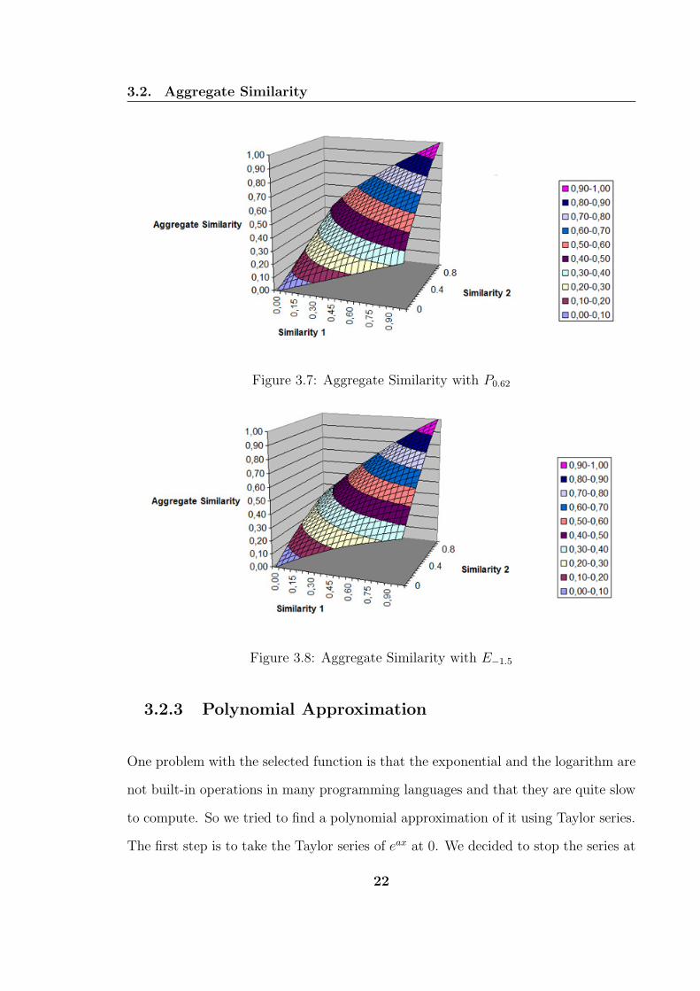
3.7 Aggregate Similarity with P0.62 . . . . . . . . . . . . . . . . . . . . . 22

3.8 Aggregate Similarity with E−1.5 . . . . . . . . . . . . . . . . . . . . . 22

ix

3.9 Approximation of the Aggregate Similarity . . . . . . . . . . . . . . . 24

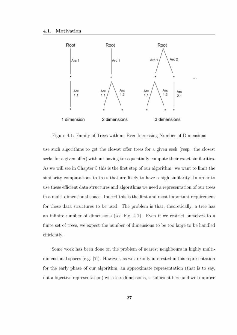
4.1 Family of Trees with an Ever Increasing Number of Dimensions . . . 27

4.2 A Fixed Tree Structure for an Apartment Rental Portal . . . . . . . . 29

4.3 Two Trees not in our Subset . . . . . . . . . . . . . . . . . . . . . . . 30

4.4 Two Trees in our Subset . . . . . . . . . . . . . . . . . . . . . . . . . 30

4.5 Examples of Corresponding Bases . . . . . . . . . . . . . . . . . . . . 31

4.6 Examples of Coordinates for Different Base Depths . . . . . . . . . . 33

4.7 Example of Inverse Bit Interleaving . . . . . . . . . . . . . . . . . . . 37

5.1 A Bartering Ring . . . . . . . . . . . . . . . . . . . . . . . . . . . . . 40

5.2 The Selection of Closest Offers . . . . . . . . . . . . . . . . . . . . . . 48

5.3 The Closure of the Ring . . . . . . . . . . . . . . . . . . . . . . . . . 49

5.4 An Ideal Agent . . . . . . . . . . . . . . . . . . . . . . . . . . . . . . 50

5.5 The Testing of the Risk . . . . . . . . . . . . . . . . . . . . . . . . . . 50

5.6 The Ring Bartering Algorithm . . . . . . . . . . . . . . . . . . . . . . 51

5.7 A Bartering Tuple Replacing 3 Bartering Pairs . . . . . . . . . . . . . 54

5.8 The Modified Closure of the Ring for Bartering Tuples . . . . . . . . 55

5.9 The Modified Testing of the Risk for Bartering Tuples . . . . . . . . . 56

6.1 The Taxonomy Part of a Project Tree in Teclantic.ca . . . . . . . . . 62

6.2 An example of Tree with its Representation . . . . . . . . . . . . . . 63

6.3 The Repartitioning of the Trees in the Buckets . . . . . . . . . . . . . 64

7.1 Behavior of the distance against the similarity . . . . . . . . . . . . . 67

7.2 Two Trees with Low Similarity and Zero Distance . . . . . . . . . . . 68

x

List of Tables

3.1 Values of a for Different 0.0/1.0 Trade Similarity Value . . . . . . . . 21

7.1 Influence of the Distance . . . . . . . . . . . . . . . . . . . . . . . . . 69

7.2 Influence of the Risk on Teclantic.ca Data . . . . . . . . . . . . . . . 70

7.3 Influence of the Risk with Random Similarity Values . . . . . . . . . 71

7.4 Computation Times . . . . . . . . . . . . . . . . . . . . . . . . . . . . 75

7.5 Computation Times and Size of the Rings . . . . . . . . . . . . . . . 76

7.6 Computation Times without Pruning . . . . . . . . . . . . . . . . . . 76

xi

Glossary

A() The adjustment function used in the weighted tree similarity algorithm.Prevents the similarity degradation with the increasing depth of the tree.

a The parameter for the aggregation function.

APa,d Polynomial approximation with degree d, of the aggregation function withparameter a.

Aik k-th arc in the i-th tree.

α Parameter in the risk function which handles the number of agents in thering.

B Base of trees.

Bn Restriction of the base of trees to the level n.

Bi i-th tree in the base B.

Bni i-th tree in the base Bn.

Dmax The maximum distance above which the algorithm will stop gatheringtrees.

Ea() The exponential based function for the aggregate similarity with parametera.

GAggSim() Generalized aggregate similarity function for bartering rings.

xii

K Key representing a tree in the OPLH.

OPLH Order Preserving Linear Hashing.

Pa() The polynomial function for the aggregate similarity with parameter a.

Rmax The maximum risk above which the algorithm will either discard the ringor will not try to add another agent to it.

Rn() The risk function.

Rn A bartering ring of size n.

S The aggregate similarity of two bartering pairs.

si i-th similarity value in a ring.

Sim() The tree similarity function.

S Multi-dimensional space corresponding to base B.

Sn Multi-dimensional space corresponding to base Bn.

Ti Notation for a Tree.

T The subset of trees we have restricted our system to.

ti Simplicity value.

TC Time complexity of our algorithm.

wi Arc weight.

xi i-th coordinate of a tree in a multi-dimensional space.

xiii

CHAPTER 1

Introduction

Similarity Match-Making is a process that helps buyers and sellers to find each other

according to the similarity of what they seek/offer. In this thesis we extend this

principle to bartering and ring bartering.

1.1 eCommerce

Before going into the details of bartering Match-Making, we will introduce some

concepts of eCommerce that are useful for our work.

In the last few decades, the importance of the Internet in our every day life has

kept increasing. Many basic tasks such as shopping can now be performed at home in

front of a computer screen. This is the field of eCommerce which, broadly conceived,

1

1.1. eCommerce

already has a long history. Indeed the early developments of eCommerce appeared in

the 1970s and 1980s with the EFT technology (Electronic Fund Transfer) and EDI

(Electronic Data Interchange) in 1984 [10, 13]. eCommerce has kept evolving since

this point, going from the stage of brochure-ware [13] in the early 1990s, that is to

say static websites that had only an informational purpose, to advanced transactional

devices that have been appearing in the last few years.

1.1.1 Web portals

Web portals are currently the main interface for Internet eCommerce users. Some

portals are company portals, they are windows of what the company is doing/provid-

ing and allow them to reach more customers. For example the store Marks & Spencer

uses this kind of web portal ( http://www.marksandspencer.com/ ). Other portals

are maintained by an external entity and are acting as interface between buyers and

sellers from different origins. Generally each is specialized in a particular area. For

instance Kasbah ( http://www.kasbah.com/ ) is centered on travels while Telzoo (

http://telezoo.com/ ) is aiming at telecommunication and networking technologies.

1.1.2 Match-Making

According to the dictionary [2], Match-Making is “The act or process of trying to bring

about a marriage for others”. In other words it has its origin in helping people to find

a suitable partner. Currently many Match-Making Web portals are actually focused

on dating. However, Match-Making has expanded throughout the years to other

areas. Telzoo, a telecommunication and networking technologies centered portal,

2

1.1. eCommerce

is using a Match-Making system to help buyers and seekers to meet. This is one

of the many examples that we can find on the Internet. The possibilities given to

the users are varying depending on the portal. For example our own Teclantic (

http://www.teclantic.ca ) gives the user the opportunity to specify the relative

importance of some aspects of his/her query.

1.1.3 Bartering

Bartering: “The practice of exchanging goods or services without using the medium

of money.” [2]

Bartering has a long history 1. It was the only way to do commerce before the

appearance of money. However, bartering has not disappeared and has made some

noticeable comebacks in the last few centuries, especially during recession periods

where money became more and more worthless such as in parts of Europe of the 1930s.

Bartering is still studied (e.g. [27, 9] for an economic perspective) and used today as

some bartering portals such as T&C Global Barter Exchange ( www.tandc-global.

com ) can testify and is even required in some particular cases. Also in our own

company merger example of cooperative work, where users are looking for other

projects to complement their own, it would be very difficult to use money.

1See [28] for more information on the history of bartering and money

3

1.2. Motivation and Approach

1.2 Motivation and Approach

Similarity Match-Making has enhanced eCcommerce in a way so that users, both

on the seller and the buyer side, can gain a great amount of time and money by

shortening both the search and the negotiation processes. Here, the Match-Making

system presents to a given user only potential partners that are likely to agree with

him/her. Consequently research in this area, trying to improve either the efficiency or

the possibilities given to the user, is of great interest. This is the aim of our similarity

Match-Making for bartering scenario system: to give the user another perspective on

Match-Making, while exploit recent techniques in similarity Match-Making to assure

efficiency.

1.2.1 Representation of Queries

For efficient product/service comparison, a suitable representation of the data is re-

quired. One of the most popular representations is the key-words/phrases widely used

by search engines, for instance. In order to carry extra information, in some systems

such as ACORN [25] weights have been added to key-words/phrases. However, in

some cases, the relationship between different features of the data is complex and

requires a hierarchical representation. For example, to describe this thesis, we would

have to give information about the university, the supervisors and the topic. The

topic is independent from the rest but the supervisors are dependent on the univer-

sity. A tree representation of queries can handle these complex relationships. To allow

such a nested representation augmented by weights we are going to use node-labelled

arc-labelled weighted trees from the AgentMatcher research group [5, 4, 31, 32] in

this thesis. More details about this representation are given in Section 2.1.2.1.

4

1.2. Motivation and Approach

1.2.2 Match-Making for Bartering Scenarios

The buyers/sellers scenario is the most widely used for the Match-Making systems

(e.g. [15, 8, 4]). The main reason is obviously because it is the most frequent situation

and the one with the easiest-to-see applications. However shifting from this classical

“client/server”-like view to a “peer-to-peer”-like view, where the buyers and sellers

both become bartering agents with something to offer as well as something they seek

(see Fig 1.1), can extend the possibilities to other areas where money is not easy

to deal with. Indeed if we want to exchange ideas or knowledge, for instance, as in

[20], we cannot use money, as it is very difficult to quantify its value. With bartered

Match-Making, we have a very natural way of dealing with this kind of “product” by

simply trading an idea or some knowledge for some other. Similarly, the Web Portal

Teclantic.ca, which is focusing on research projects, was particularly adapted for this

approach.

Figure 1.1: The Bartering Scenario

5

1.3. Objectives

1.2.3 Ring Bartering

The main focus in Match-Making is to find the best match between different agents of

the virtual market place [8, 19, 30, 23, 29, 15]. However, limiting the potential deals

to two agents is a strong restriction. It does not matter in the case of buying/selling

scenarios but in the case of bartering it does as it is not always likely that a match

is going to be found for a particular offer/seek pair. On the contrary, it is very likely

to find situations where a strong match will be found for one side of the deal. For

example, an agent is seeking for an apartment in Halifax and another agent is offering

one there. But the other part of the trade may not match at all. The first agent could

offer an apartment in Tregun while the second one is seeking one in Toronto. Adding

more agents to the trade can improve the global satisfaction of all the agents. A third

agent could come into the previous trade offering an apartment in Toronto and looking

for one in Tregun. Separately paired, none of this agents could match satisfactorily,

but all of them together will, and thus will form a bartering ring.

1.3 Objectives

This thesis aims to develop an advanced similarity Match-Making system centered

on bartering scenarios. The main objectives are as follows:

• To develop techniques for bartered Match-Making.

• To develop techniques for ring bartering.

• To apply these techniques to Teclantic.ca for testing them.

6

1.4. Organization of the Thesis

One of the main concern that has driven our work is the computation time. This thesis

aims at finding efficient ways of providing agents with the best potential partners.

1.4 Organization of the Thesis

This thesis is organized as follows. Chapter 2 presents some background on similarity

Match-Making and bartering, introducing the arc-labelled weighted tree representa-

tion of queries that is going to be used by our system. The concept of bartering trees

is presented in Chapter 3. Chapter 4 presents an approximate representation of our

trees in a multi-dimensional space. The ring bartering algorithm is given in Chap-

ter 5. Chapter 6 presents an application of our system in the research area. Finally,

Chapter 7 discusses some tests of our system.

7

CHAPTER 2

Match-Making and Bartering

Coincidently with the development of the Internet, eCommerce has become more

and more important in our everyday life. Being more than mere display windows,

company websites and web portals are now a standard means of reaching customers

or finding providers. Virtual market places are emerging all over the world, growing

in number and importance. The necessity of powerful tools to help users navigate

through these market places is thus also increasing. It is not possible anymore to just

display lists of offers and/or seeks to users, as the number of potential partners is

rising drastically.

To help users, multi-agents systems have been developed. These systems repre-

sent the user by a virtual agent who is going to communicate with the other agents

of the e-Marketplace by exchanging their knowledge of their users’ preferences. The

aim is to find the product/service closest (most similar) to a user’s desire. Many algo-

8

2.1. Match-Making

rithms have been designed for this purpose. Research has also been done on bartering

with applications in various areas.

2.1 Match-Making

Extensive research has been conducted on Match-Making [8, 19, 30, 23, 29]. IBM’s

Websphere Matchmaking Environment was one of the first to emphasize the match-

making between a demand and a supply, for commercial use. The matching engine

underneath uses properties and rules which describe the supplies/demands and per-

forms comparisons of the properties and verifications of the rules.

2.1.1 Agent-Mediated eCommerce System with Decision

Analysis Features

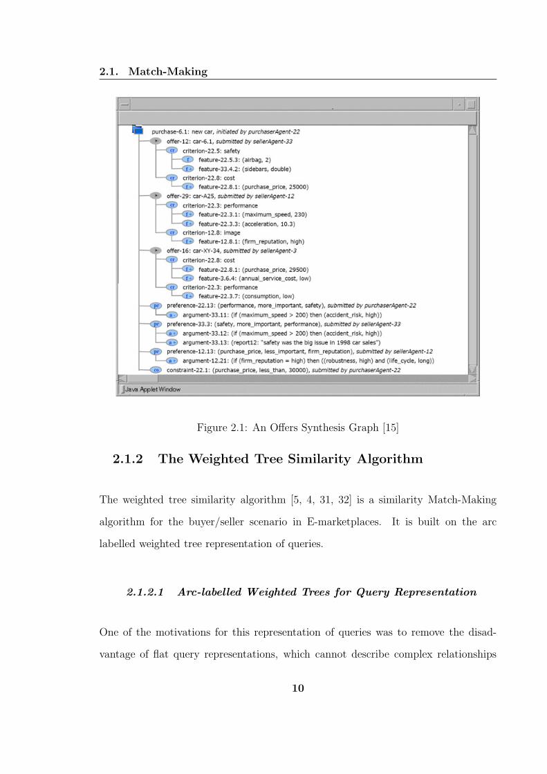
Another more recent approach is in [15] where the purchase and the potential offers

are represented in a single Offer synthesis graph. This graph regroups criteria and

related features as well as preferences with related arguments, as illustrated in Fig 2.1.

From this figure we can see that this graph is actually a tree.

The graph is built by the purchaser agent and updated for a given time limit.

Then the user interacts with the graph to activate or deactivate nodes of the graph.

The system also checks for conflicts and inconsistencies and deactivates nodes accord-

ingly in case of constraint violations, or asks the user to make a decision for conflicting

preferences. Then the system gives a score to each offer using a weighting schema

based on the user preferences.

9

2.1. Match-Making

Figure 2.1: An Offers Synthesis Graph [15]

2.1.2 The Weighted Tree Similarity Algorithm

The weighted tree similarity algorithm [5, 4, 31, 32] is a similarity Match-Making

algorithm for the buyer/seller scenario in E-marketplaces. It is built on the arc

labelled weighted tree representation of queries.

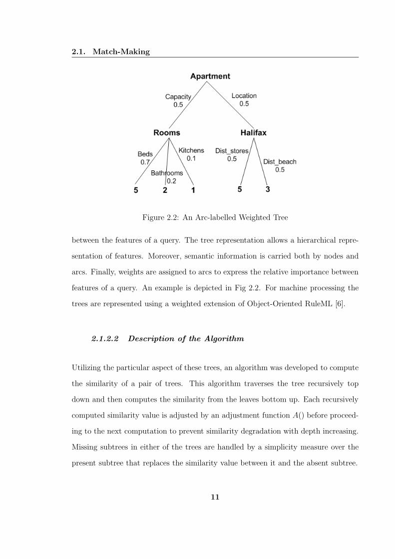
2.1.2.1 Arc-labelled Weighted Trees for Query Representation

One of the motivations for this representation of queries was to remove the disad-

vantage of flat query representations, which cannot describe complex relationships

10

2.1. Match-Making

Figure 2.2: An Arc-labelled Weighted Tree

between the features of a query. The tree representation allows a hierarchical repre-

sentation of features. Moreover, semantic information is carried both by nodes and

arcs. Finally, weights are assigned to arcs to express the relative importance between

features of a query. An example is depicted in Fig 2.2. For machine processing the

trees are represented using a weighted extension of Object-Oriented RuleML [6].

2.1.2.2 Description of the Algorithm

Utilizing the particular aspect of these trees, an algorithm was developed to compute

the similarity of a pair of trees. This algorithm traverses the tree recursively top

down and then computes the similarity from the leaves bottom up. Each recursively

computed similarity value is adjusted by an adjustment function A() before proceed-

ing to the next computation to prevent similarity degradation with depth increasing.

Missing subtrees in either of the trees are handled by a simplicity measure over the

present subtree that replaces the similarity value between it and the absent subtree.

11

2.1. Match-Making

The formula expressing the similarity at a given level, with the weights wji adding

up to 1.0 for a given j, is the following:

Sim(T1, T2) =∑

(

A(si) ·w1i + w2i

2

)

(2.1)

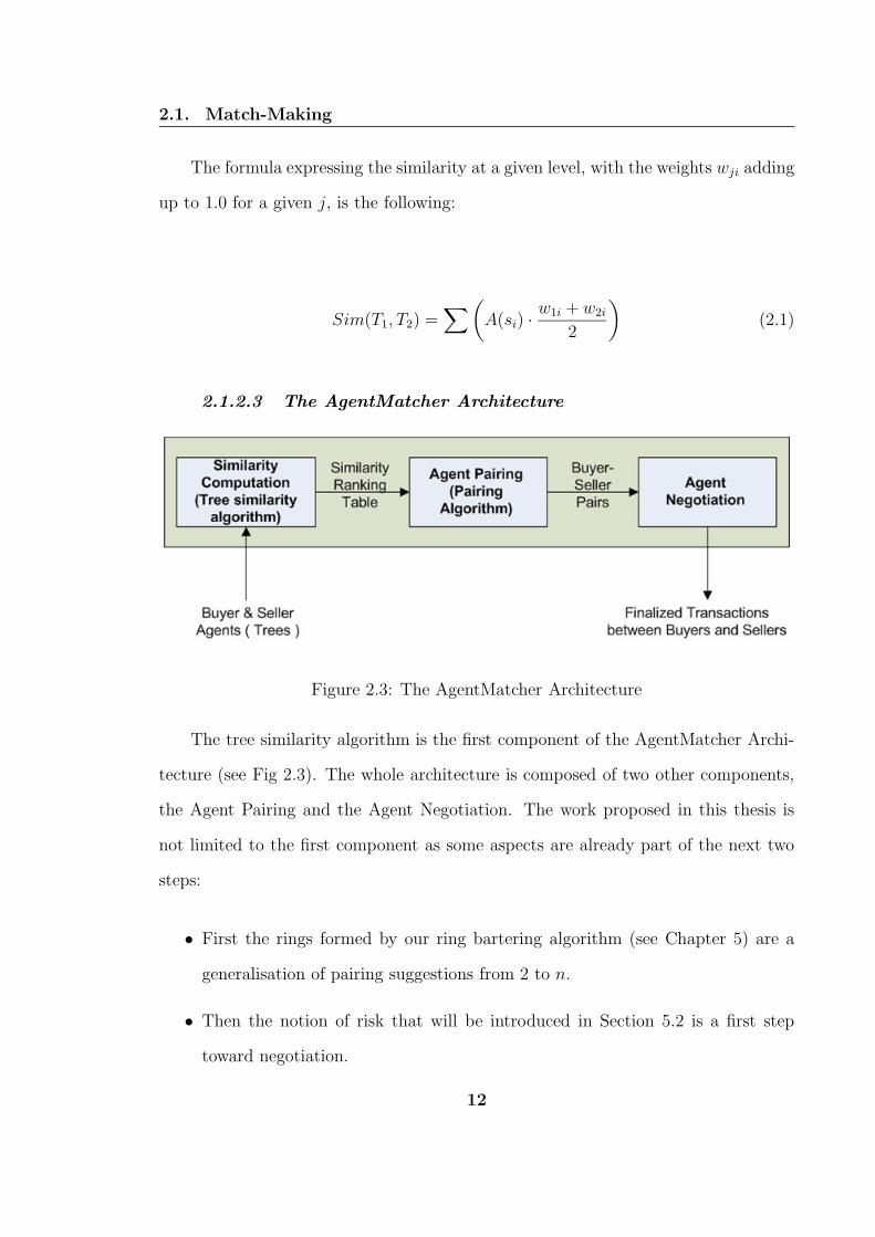
2.1.2.3 The AgentMatcher Architecture

Figure 2.3: The AgentMatcher Architecture

The tree similarity algorithm is the first component of the AgentMatcher Archi-

tecture (see Fig 2.3). The whole architecture is composed of two other components,

the Agent Pairing and the Agent Negotiation. The work proposed in this thesis is

not limited to the first component as some aspects are already part of the next two

steps:

• First the rings formed by our ring bartering algorithm (see Chapter 5) are a

generalisation of pairing suggestions from 2 to n.

• Then the notion of risk that will be introduced in Section 5.2 is a first step

toward negotiation.

12

2.2. Bartering

2.2 Bartering

Bartering systems have been proposed using different approaches and restrictions.

The trade balance problem, that is to say trying to make profitable deals while keeping

the balance of every user close to zero is discussed in [12]. The balance of the user

is artificially created by using trade dollars as intermediate in the bartering process.

Instead of trying to perform direct exchanges of goods between users, the system

performs one way deals ( e.g. user1 is buying an amount A of goods for a price P

in trade dollars from user2 ). Then the system will try to bring back the balance of

user1 and user2 to zero by making other deals with other users. This can be seen

as what we call a ring bartering process but delayed in time. However, one major

requirement of this approach is to be able to quantify and/or evaluate goods in the

“bartering pool”. This is not always possible, e.g. when dealing with people and

information as in [20].

In [20], the aim is to improve the global knowledge of agents by sharing/exchang-

ing cases. The decision of making a deal or not is done by checking whether a value

called ICB (Individual Case Bias) is decreasing or not. This approach is not quite

related to eCommerce as in the latter the aim is not to improve a global knowledge

but to satisfy two parties: the seller and the buyer.

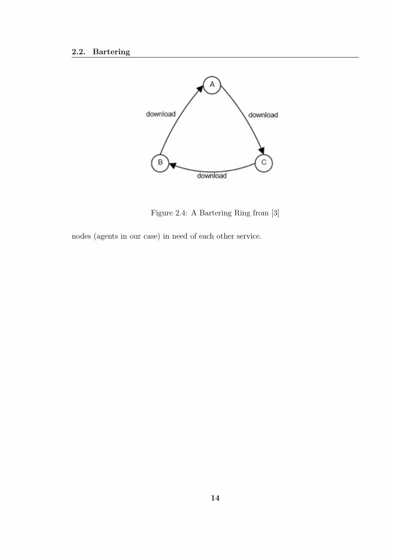
2.2.1 Ring Bartering

We did not find relevant work done on Ring Bartering for eCommerce. However 3

nodes Bartering Rings for Peer to Peer applications (see Fig 2.4) are used in [3]. This

work starts from the same assumptions as ours, namely that it is difficult to find two

13

2.2. Bartering

Figure 2.4: A Bartering Ring from [3]

nodes (agents in our case) in need of each other service.

14

CHAPTER 3

Bartering Trees

3.1 Bartering Trees

The first step to deal with Bartering Scenarios is to shift the “client/server”-like

buyer/seller view to a “peer-to-peer”-like bartering agent view. The former uses a

single tree to represent an agent: a seek tree in the case of a buyer and an offer tree

for a seller. With bartering agents, we need two trees for each agent (see Fig. 3.1),

one for its offer and one for its seek, as each bartering agent is at the same time a

potential buyer as well as a potential seller.

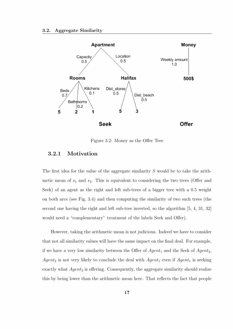
This concept of bartering trees can be seen as the generalisation of the usual goods

for money deal. Indeed it is always possible to represent money as a degenerated tree

and have this tree as the offer of the first bartering agent (see Fig. 3.2), the former

15

3.2. Aggregate Similarity

Figure 3.1: Bartering Tree Pair

buyer, and a similar one as the seek of the second bartering agent, the former seller.

3.2 Aggregate Similarity

When dealing with bartering scenarios, we are faced with two levels of similarity.

First we have the similarity values between, on one side, the offer of Agent1 and the

seek of Agent2 and, on the other side, the seek of Agent1 and the offer of Agent2.

The second level of similarity is the aggregate similarity between the two pairs. This

similarity S is to be computed from the two previous ones s1 and s2. This process

is to be performed with caution as S is the final result that the user will obtain.

Figure 3.3 illustrates the two levels of similarity for two bartering pairs.

16

3.2. Aggregate Similarity

Figure 3.2: Money as the Offer Tree

3.2.1 Motivation

The first idea for the value of the aggregate similarity S would be to take the arith-

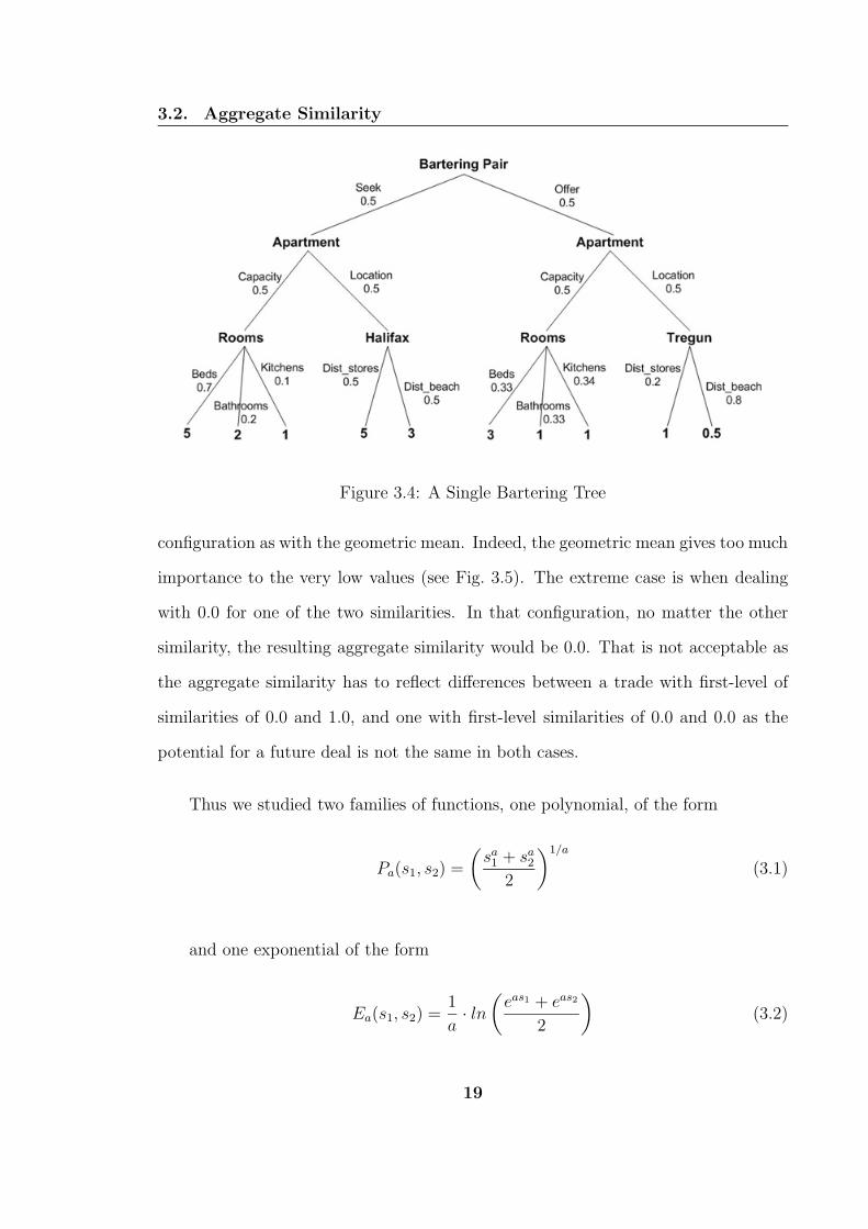
metic mean of s1 and s2. This is equivalent to considering the two trees (Offer and

Seek) of an agent as the right and left sub-trees of a bigger tree with a 0.5 weight

on both arcs (see Fig. 3.4) and then computing the similarity of two such trees (the

second one having the right and left sub-tree inverted, so the algorithm [5, 4, 31, 32]

would need a “complementary” treatment of the labels Seek and Offer).

However, taking the arithmetic mean is not judicious. Indeed we have to consider

that not all similarity values will have the same impact on the final deal. For example,

if we have a very low similarity between the Offer of Agent1 and the Seek of Agent2,

Agent2 is not very likely to conclude the deal with Agent1 even if Agent1 is seeking

exactly what Agent2 is offering. Consequently, the aggregate similarity should realize

this by being lower than the arithmetic mean here. That reflects the fact that people

17

3.2. Aggregate Similarity

Figure 3.3: Two levels of similarity

try to maximize their Seek similarity (the other’s Offer similarity), not their Offer

similarity (the other’s Seek similarity). So, the aggregate similarity should not be a

linear combination of s1 and s2: if any of these two component similarities approaches

0.0, the aggregate similarity should also approach 0.0. If we take the most extreme

case, with the arithmetic mean the aggregate similarity for s1 = 0.0 and s2 = 1.0

would be 1

2(0.0 + 1.0) = 0.5, that is to say the same value as if s1 = s2 = 0.5 =

1

2(0.5+0.5). This appears not judicious as the agents involved in the potential 0.0/1.0

deal are clearly going to behave differently from those in the potential 0.5/0.5 deal.

3.2.2 Aggregation Function

In the context of discussion in Section 3.2.1 we had to find another way of combination

for the aggregate similarity. The first idea was to try some non arithmetic means.

When dealing with means that are not linear what comes to mind at first are the

harmonic ( 1

1/x+1/y) and the geometric (

√x · y ) means. The former one is not

applicable as we would have a problem when dealing with 0.0. It would still be

possible to make a continuity extension however we would then end up in the same

18

3.2. Aggregate Similarity

Figure 3.4: A Single Bartering Tree

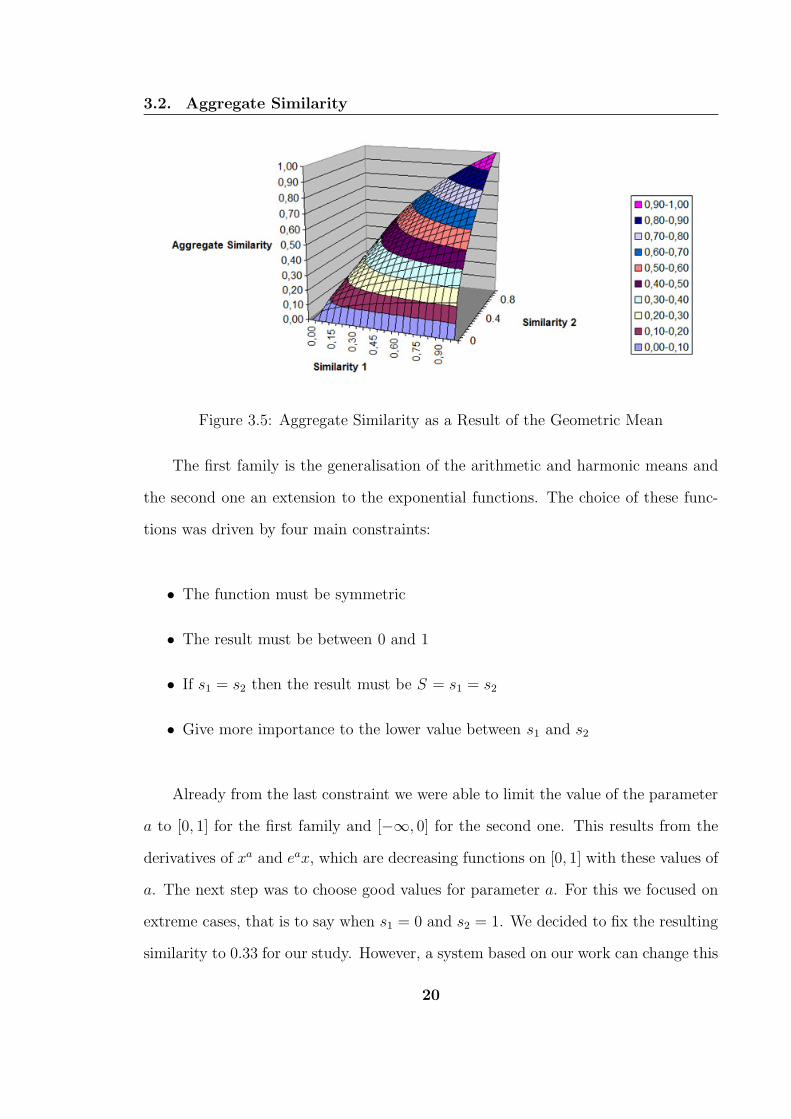
configuration as with the geometric mean. Indeed, the geometric mean gives too much

importance to the very low values (see Fig. 3.5). The extreme case is when dealing

with 0.0 for one of the two similarities. In that configuration, no matter the other

similarity, the resulting aggregate similarity would be 0.0. That is not acceptable as

the aggregate similarity has to reflect differences between a trade with first-level of

similarities of 0.0 and 1.0, and one with first-level similarities of 0.0 and 0.0 as the

potential for a future deal is not the same in both cases.

Thus we studied two families of functions, one polynomial, of the form

Pa(s1, s2) =

(

sa1 + sa

2

2

)1/a

(3.1)

and one exponential of the form

Ea(s1, s2) =1

a· ln(

eas1 + eas2

2

)

(3.2)

19

3.2. Aggregate Similarity

Figure 3.5: Aggregate Similarity as a Result of the Geometric Mean

The first family is the generalisation of the arithmetic and harmonic means and

the second one an extension to the exponential functions. The choice of these func-

tions was driven by four main constraints:

• The function must be symmetric

• The result must be between 0 and 1

• If s1 = s2 then the result must be S = s1 = s2

• Give more importance to the lower value between s1 and s2

Already from the last constraint we were able to limit the value of the parameter

a to [0, 1] for the first family and [−∞, 0] for the second one. This results from the

derivatives of xa and eax, which are decreasing functions on [0, 1] with these values of

a. The next step was to choose good values for parameter a. For this we focused on

extreme cases, that is to say when s1 = 0 and s2 = 1. We decided to fix the resulting

similarity to 0.33 for our study. However, a system based on our work can change this

20

3.2. Aggregate Similarity

0.0/1.0 trade a for Pa a for Ea

0.1 0.3 -70.25 0.5 -2.50.33 0.62 -1.50.5 1 n/a (or 0 by extension)

Table 3.1: Values of a for Different 0.0/1.0 Trade Similarity Value

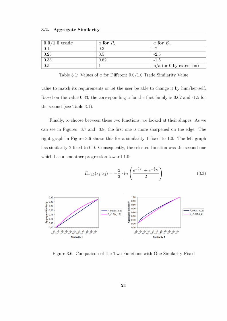
value to match its requirements or let the user be able to change it by him/her-self.

Based on the value 0.33, the corresponding a for the first family is 0.62 and -1.5 for

the second (see Table 3.1).

Finally, to choose between these two functions, we looked at their shapes. As we

can see in Figures 3.7 and 3.8, the first one is more sharpened on the edge. The

right graph in Figure 3.6 shows this for a similarity 1 fixed to 1.0. The left graph

has similarity 2 fixed to 0.0. Consequently, the selected function was the second one

which has a smoother progression toward 1.0:

E−1.5(s1, s2) = −2

3· ln(

e−3

2s1 + e−

3

2s2

2

)

(3.3)

Figure 3.6: Comparison of the Two Functions with One Similarity Fixed

21

3.2. Aggregate Similarity

Figure 3.7: Aggregate Similarity with P0.62

Figure 3.8: Aggregate Similarity with E−1.5

3.2.3 Polynomial Approximation

One problem with the selected function is that the exponential and the logarithm are

not built-in operations in many programming languages and that they are quite slow

to compute. So we tried to find a polynomial approximation of it using Taylor series.

The first step is to take the Taylor series of eax at 0. We decided to stop the series at

22

3.2. Aggregate Similarity

the eighth order.

1 + ax +1

2a2x2 +

1

6a3x3 +

1

24a4x4 +

1

120a5x5 +

1

720a6x6 +

1

5040a7x7 + O(x8)

Then we have to take the Taylor series of ln(1 + x) at 0. Here again stopped at

order eight.

x − 1

2x2 +

1

3x3 − 1

4x4 +

1

5x5 − 1

6x6 +

1

7x7 + O(x8)

Finally, substitute the x in the previous formula by the combination of the first

one applied to s1 and s2, divided by 2 and -1 ( because it was a development of

ln(1 + x) and not ln(x) ). The resulting two variable polynomial, of degree 49 is

relevant only up to degree seven as the two Taylor series were at order eight. Of

course this approximation has to be tested because these two series are only relevant

around x = 0 and here we have values that are going up to 1.

We have tested with the degree 2 polynomial function:

APa,2(s1, s2) =1

8as2

1 +1

8as2

2 −1

4as1s2 +

1

2s1 +

1

2s2 (3.4)

From this function with a = −1.5 we obtained a maximum deviation from the

original function of 0.02 (4.67%) for only the two extreme values and an average

deviation of 0.35% (See Figure 3.9).

As a variation of 0.02 for a similarity value will not change the interpretation of

the results, this approximation appears acceptable. The next approximation would

23

3.2. Aggregate Similarity

Figure 3.9: Approximation of the Aggregate Similarity

require a degree 4 polynomial as there are no degree 3 terms, and so the increased

computation time appears not to be worth the resulting gain ( maximum deviation

of 0.69%, average deviation of 0.03% ).

The resulting degree 2 and 4 polynomials for a = −1.5 are the following:

AP−1.5,2(s1, s2) = − 3

16(s2

1 + s2

2) +3

8s1s2 +

1

2(s1 + s2) (3.5)

AP−1.5,4(s1, s2) =9

512(s4

1 + s4

2) −9

128(s3

1s2 + s1s3

2) +27

256s2

1s2

2

− 3

16(s2

1 + s2

2) +3

8s1s2 +

1

2(s1 + s2) (3.6)

Intuitively, note that in both cases, reading these sums from right to left, we

take the arithmetic mean of s1 and s2, add 3/8th of their product (while the geo-

metric mean is the square root of their product), and subtract a combination of their

squares. While the degree 2 polynomial uses this as the similarity value, the degree 4

24

3.3. Summary and Remarks

polynomial performs three further corrective additions/subtractions on the arithmetic

mean.

3.3 Summary and Remarks

We have defined the concept of bartering trees which constitute a pair of trees, one for

the agent’s offer and one for his/her seek. Then we defined the aggregate similarity.

This value, describing the similarity between two bartering pairs, is computed from

the similarity values of the first offer with the second seek and of the first seek with

the second offer. We did not just use the arithmetic mean as we think it is not giving

enough importance to low similarity values, which are more likely to make the future

negotiation steps fail. Instead we found an exponential based function. We finally

gave a polynomial approximation to prevent computation time losses.

The weighting schema presented in this chapter to combine the two first-level

similarity values could also be applied within the similarity algorithm. We are cur-

rently using the arithmetic mean to combine the recursively computed similarities at

every inner node of the tree structure. We could replace this arithmetic mean by our

aggregation function (or its generalized form - see Section 5.1.2) for the same reasons

we stated at the beginning of this chapter.

25

CHAPTER 4

Tree Approximation in aMulti-Dimensional Space

In this chapter we propose a representation approximating arc-labelled node-labelled

weighted trees in a multi-dimensional space. We define a family of representations

with less and less dimensions resulting in more coarse-grained approximations. We

then expose the Order Preserving Linear Hashing data-structure which provides us

with an efficient way of performing range queries in our multidimensional space.

4.1 Motivation

Many multi-dimensional data-structures and algorithms exist to efficiently handle

range queries and/or the nearest neighbours problem [26]. In our system we want to

26

4.1. Motivation

Figure 4.1: Family of Trees with an Ever Increasing Number of Dimensions

use such algorithms to get the closest offer trees for a given seek (resp. the closest

seeks for a given offer) without having to sequentially compute their exact similarities.

As we will see in Chapter 5 this is the first step of our algorithm: we want to limit the

similarity computations to trees that are likely to have a high similarity. In order to

use these efficient data structures and algorithms we need a representation of our trees

in a multi-dimensional space. Indeed this is the first and most important requirement

for these data structures to be used. The problem is that, theoretically, a tree has

an infinite number of dimensions (see Fig. 4.1). Even if we restrict ourselves to a

finite set of trees, we expect the number of dimensions to be too large to be handled

efficiently.

Some work has been done on the problem of nearest neighbours in highly multi-

dimensional spaces (e.g. [7]). However, as we are only interested in this representation

for the early phase of our algorithm, an approximate representation (that is to say,

not a bijective representation) with less dimensions, is sufficient here and will improve

27

4.2. Tree Representation in a Multi-dimensional Space

the speed of our system.

4.2 Tree Representation in a Multi-dimensional

Space

We are now going to detail how to represent an arc-labelled node-labelled weighted

tree in a multi-dimensional space. The first step is to define the subset of the set of

all possible arc-labelled node-labelled weighted trees to work with. Such subsetting

corresponds to constructing tree instances according to a tree schema, as already

explored in AgentMatcher’s eLearning application [11] and in Teclantic.ca. We will

assume that the set of trees we are working with has, for a given set of arcs, a unique

set of corresponding inner nodes. That is to say that a given arc will always come

from the same node, and will always go to the same node, except for the leaf level (see

Definition 4.2.1 and Figures 4.3, 4.4). The representation would still work without

this restriction, but the number of dimensions would greatly increase. We will present

a solution in section 4.2.3 to deal with trees not from this set without increasing the

number of dimensions. Finally, this restriction may appear very strict in theory, but

in practice it is very often the case that the structure of the trees is more or less fixed

with only the number of arcs and the leaves varying (e.g. Figure 4.2).

Definition 4.2.1 (path-to-node persistant trees) Let T be a set of trees such

that for all trees Ti and Tj ∈ T if two arcs Aik ∈ Ti and Ajl ∈ Tj have the same arc

label and are on corresponding paths from their respective roots (in terms of arc labels

and node labels), then either they have the same child node label or they point to a

leaf.

28

4.2. Tree Representation in a Multi-dimensional Space

Figure 4.2: A Fixed Tree Structure for an Apartment Rental Portal

4.2.1 Definition of the Multi-dimensional Space

We will now define the space, where our trees will be represented by defining the

corresponding base.

Definition 4.2.2 For all possible paths from a root to a leaf in the tree schema of

the set of trees T , we define a unary tree Bi. This tree is the restriction of the tree

schema to this path with no value on the leaf and all weights set to 1.0. Let B be the

set of all Bi. B is the base for the set T in the k-dimensional space S where k is the

number of Bi.

This is the first base of our family. The one with the least approximation. Indeed

we only have an approximation on the leaf level. If we want an exact representation,

we need to keep the information on the leaves. We will see in section 4.2.3 how to deal

with this without increasing the number of dimensions. The other bases are defined

as follows:

29

4.2. Tree Representation in a Multi-dimensional Space

Figure 4.3: Two Trees not in our Subset

Figure 4.4: Two Trees in our Subset

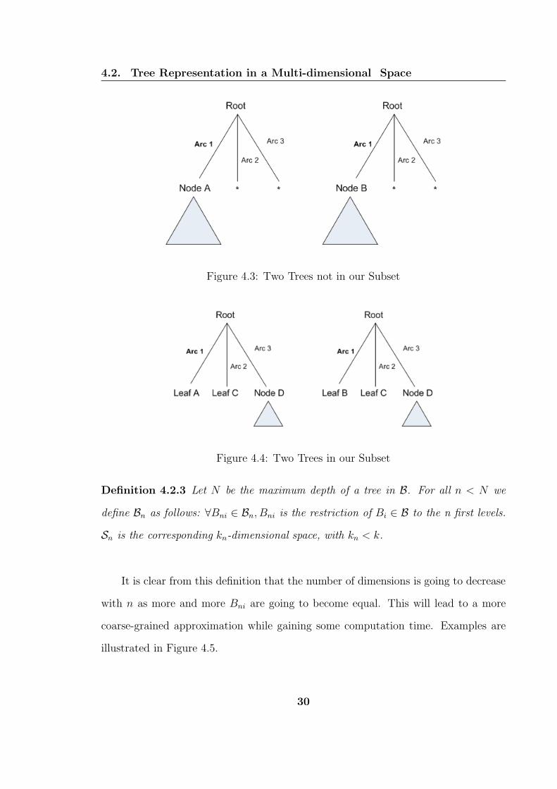
Definition 4.2.3 Let N be the maximum depth of a tree in B. For all n < N we

define Bn as follows: ∀Bni ∈ Bn, Bni is the restriction of Bi ∈ B to the n first levels.

Sn is the corresponding kn-dimensional space, with kn < k.

It is clear from this definition that the number of dimensions is going to decrease

with n as more and more Bni are going to become equal. This will lead to a more

coarse-grained approximation while gaining some computation time. Examples are

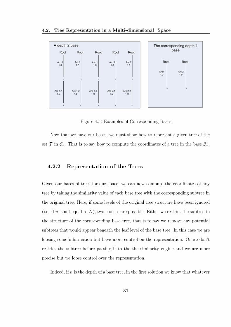
illustrated in Figure 4.5.

30

4.2. Tree Representation in a Multi-dimensional Space

Figure 4.5: Examples of Corresponding Bases

Now that we have our bases, we must show how to represent a given tree of the

set T in Sn. That is to say how to compute the coordinates of a tree in the base Bn.

4.2.2 Representation of the Trees

Given our bases of trees for our space, we can now compute the coordinates of any

tree by taking the similarity value of each base tree with the corresponding subtree in

the original tree. Here, if some levels of the original tree structure have been ignored

(i.e. if n is not equal to N), two choices are possible. Either we restrict the subtree to

the structure of the corresponding base tree, that is to say we remove any potential

subtrees that would appear beneath the leaf level of the base tree. In this case we are

loosing some information but have more control on the representation. Or we don’t

restrict the subtree before passing it to the the similarity engine and we are more

precise but we loose control over the representation.

Indeed, if n is the depth of a base tree, in the first solution we know that whatever

31

4.2. Tree Representation in a Multi-dimensional Space

the (n+1)-th level is, if the first n levels of two trees are identical, they will have the

same representation. In the second case, two trees can have different representations

even if the first n levels are identical, but it is very difficult to tell how the representa-

tion will evolve. Two totally different trees at the (n + 1)-th level can have the same

representation and two nearly equal trees can have a different one. The explanation

of this comes from the fact that the information we add here is only the structure of

the (n + 1)-th level and not the values. So we are more precise but must be cautious

while interpreting the results.

Consequently, if we apply the similarity computation the i-th coordinate for a

given tree will be, in case of a one level tree base with wi being the weight of the

corresponding arc in the original tree, ti the simplicity of a potential missing subtree

(or 1 otherwise) and A() the adjustment function

xi = wi+1

2· A(ti)

For a two level tree base we would have

xi = wi1+1

2· A(wi2+1

2· A(ti))

The formula for recursively computed similarities sik is

xi = wik+1

2· A(sik+1)

4.2.3 Keeping Information on Nodes and Leaves

The first restriction made on our trees when computing their coordinates, that is to

say ignoring the node and leaf values, can be worked around without a great loss in

32

4.2. Tree Representation in a Multi-dimensional Space

Figure 4.6: Examples of Coordinates for Different Base Depths

computation time. Indeed we ignored these values because, as the current similarity

algorithm is defined, there is no way to distinguish two different values from two

others: the similarity between two leaves is either 0 or 1. Consequently, we need to

have in order to get a unique representation in the space, a base tree for each possible

value. However, recent work on the algorithm [5] showed that in some cases we could

compute a similarity ranging between 0 and 1 for two leaves by using a local similarity

measure. For example two price values or two dates. Consequently, every time we

can compute such a local similarity between leaves we can keep the information in

these leaves, without adding any dimension to the base. All we have to do is set the

base tree leaf value to a default value such as the mean value if it exists. This could

also be extended to inner nodes for identical arcs that lead to different node values.

Moreover, we can extend this principle to all finite sets of values. Indeed, some-

33

4.3. Notion of Distance

times it may not be possible to compute easily a similarity between values. For

example, if we take towns, one could take the similarity between their population,

or their distance from one point or many other parameters. None of them would be

really accurate. One solution would be, if the set of possible values is finite, to create

a table of values, incorporated into the system that will give the “similarity” value

between every pair.

These methods will increase the precision in the computation of the distance

without adding any dimension and thus computation time. Of course we will still

have the computation time of the local similarity.

4.3 Notion of Distance

The aim of this representation of queries is to perform range searches to make a first

selection among all the possible choices. In other words, we want to select all the

trees that are within a given distance of the query point. We are now going to define

the distance between two trees in our multi-dimensional space.

4.3.1 Definition

We define the square of the distance between two trees as follows (n is the dimension

of the space). It is the usual Euclidean distance between two points

||T1, T2||2 =

n∑

i=1

(xi − x′

i)2

34

4.3. Notion of Distance

Consequently for a one level tree base the expression of the distance between two

trees becomes

||T1, T2||2 =n∑

i=1

(

wi + 1

2· A(ti) −

w′

i + 1

2· A(t′i)

)2

.

4.3.2 Behavior

If T1 = T2 then ∀i, wi = w′

i and ti = t′i. Consequently, all the terms in the sum

become null and the distance is 0, which is what we expected in such a case.

On the other hand, if T1 and T2 are very different, for most values of i either ti or

t′i will be null (that is to say that most of the branches existing in the first tree will

not exist in the second one and vice versa) and consequently for those values of i, one

of the terms of the subtraction will be null and the resulting term will be of greater

importance. So we can see that the more different the two trees are, the greater is

their distance.

Of course when taking a base less deep than the real trees, it is possible to have

a zero distance for trees that are not similar at all because of lower levels that are not

taken into account. However, this does not matter, as such trees will be discarded

very soon in the algorithm (see Chapter 5). The most important fact is that for high

similarity values the distance will be low, no matter the depth of the base.

This confirms the choice of our definition of distance and, most of all, of our

choice of tree representation in a finite space as this was the main constraint. In

Chapter 7 we will discuss some test results of the distances and the corresponding

similarities supporting our choice.

35

4.4. Order Preserving Linear Hashing

4.4 Order Preserving Linear Hashing

Order Preserving Linear Hashing (OPLH) is a variation of the Linear Hashing data

structure from Litwin [18] that handles range queries more efficiently. We are going

to use this data-structure to retrieve trees in the first phase of our algorithm.

4.4.1 Principle

The OPLH is a bucket based data-structure without directory. It grows or shrinks

dynamically while data are being inserted or deleted. Each piece of data is represented

by a key K. This key is generated by the inversed bit interleaving operation (see

Figure 4.7). Then the following hashing function is used to determine which bucket

the data is to be stored in.

h(K) = K mod 2n+1 if h(K) < number of buckets

h(K) = K mod 2n otherwise(4.1)

The splitting process is controlled by a storage utilization factor. Overflow buck-

ets are assigned when a bucket is full.

4.4.2 Range Queries

Range queries are performed by visiting the buckets that intersect with the query.

These buckets are found by splitting recursively the space while checking whether the

36

4.5. Remarks

Figure 4.7: Example of Inverse Bit Interleaving

current subspace is outside, inside, or intersecting with the query.

In our algorithm, we define the query by a maximum distance (defined as in

Section 4.3.1) above which the trees must not be retrieved.

Then in the last phase of the query, we have to check the points in the buckets

to keep only those below the maximum authorized distance. We can also decide to

keep all the trees stored in the buckets that intersect with the query. This will speed

up the selection process but will increase the number of trees that will be selected.

Moreover, we loose some control on the selected trees.

4.5 Remarks

• Depending on the system where our algorithm will be implemented, some vari-

ations of Linear Hashing and/or OPLH could be applied. Some variations that

use a key vector instead of a single key are given in [16, 21, 22]. The choice of

the hash function according to the key distribution is discussed in [24]. This

37

4.5. Remarks

requires knowledge of the latter but can improve performance by ensuring a

better repartition among the buckets. Finally, the local order preserving prop-

erty of OPLH is extended to global order preserving in [14]. That is to say that

not only points in the same buckets will be close to each other, but also points

in adjacent buckets will not be too far apart.

• This whole chapter is independent of our ring bartering system and contains

results that can be used for other indexing purposes. For example the retrieval

of categories of trees in the database with a single query.

38

CHAPTER 5

Ring Bartering

In this chapter we describe our Ring Bartering algorithm. We first make some prelim-

inary remarks before describing the notion of risk. Then we proceed to the description

of our algorithm before extending it to bartering tuples.

5.1 Preliminaries

In the rest of this chapter, we are going to assume, without loss of generality, that we

will start from a seek. That is to say that the initial query will be made from a seek.

We will show later that starting from an offer will give the same results.

Except where mentioned otherwise, the labelling of the agents in this chapter are

relative to a given ring. For example, Agent1 is the first agent in the current ring.

39

5.1. Preliminaries

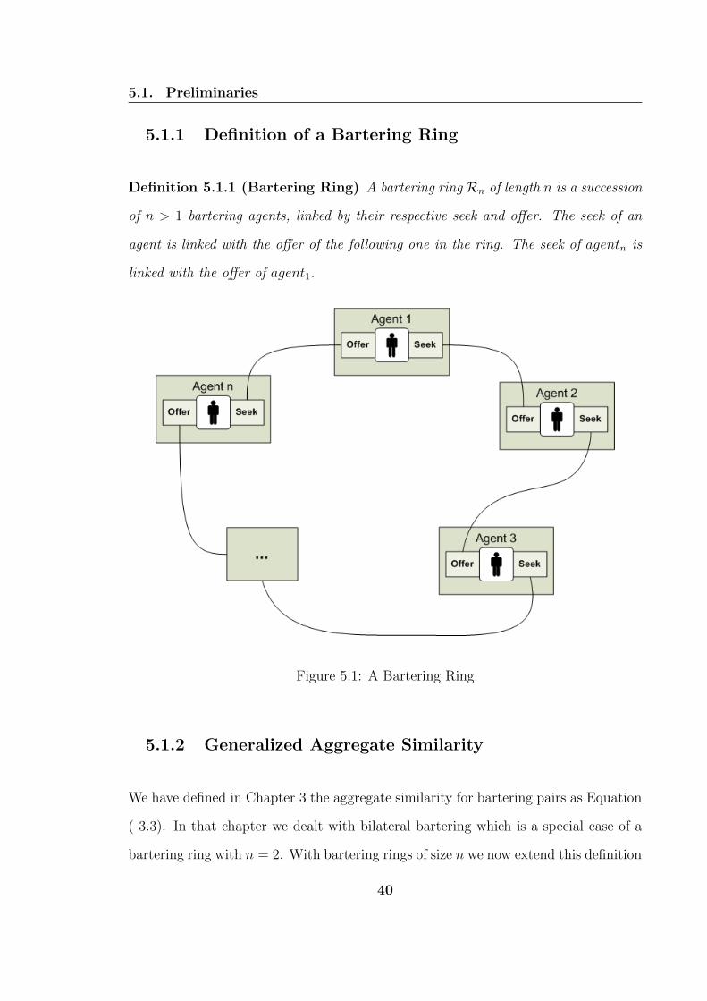
5.1.1 Definition of a Bartering Ring

Definition 5.1.1 (Bartering Ring) A bartering ring Rn of length n is a succession

of n > 1 bartering agents, linked by their respective seek and offer. The seek of an

agent is linked with the offer of the following one in the ring. The seek of agentn is

linked with the offer of agent1.

Figure 5.1: A Bartering Ring

5.1.2 Generalized Aggregate Similarity

We have defined in Chapter 3 the aggregate similarity for bartering pairs as Equation

( 3.3). In that chapter we dealt with bilateral bartering which is a special case of a

bartering ring with n = 2. With bartering rings of size n we now extend this definition

40

5.2. Notion of Risk

to more than two similarity values in a natural manner. This generalized aggregate

similarity is the value that describes the similarities between all consecutive seeks and

offers in the ring:

GAggSim(s1, ...sn) = −2

3· ln(

∑ni=1

e−3

2si

n

)

. (5.1)

5.2 Notion of Risk

When speaking about bartering, and making deal in general, there is always a risk

that one participant in a potential deal will not agree with the terms of the deal.

Especially if what he/she would receive does not match very well with what he/she

is seeking. Other reasons could interfere, such as a sudden change of mind and a

financial problem. The more participants in a trade, the more likely such behavior is

going to happen. Consequently, giving risk measures as well as the similarity values of

potential deals is a valuable information that will allow users to weigh the similarity

values that are given to them. Most importantly, this information will be key to

efficient pruning during the ring construction process (see Section 5.3).

5.2.1 Definition

There are two main aspects that can increase the risk of a deal:

• The number of participants in the deal

41

5.2. Notion of Risk

• The similarities between the corresponding seeks and offers that are involved in

the deal.

Moreover, very low similarity values should have a great impact on the risk mea-

sure as a very low similarity value between a seek and an offer in the ring is very

likely to make the whole trade collapse even if the generalized aggregate similarity

is high. A zero valued similarity somewhere in the ring should give the value of one

to the risk value. Consequently, the harmonic mean, which is the lowest of the usual

means seems a good choice. Of course we will have to make a continuity extension

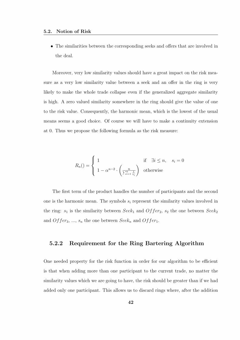
at 0. Thus we propose the following formula as the risk measure:

Rn() =

1 if ∃i ≤ n, si = 0

1 − αn−2 ·(

nPn

i=1

1

si

)

otherwise

The first term of the product handles the number of participants and the second

one is the harmonic mean. The symbols si represent the similarity values involved in

the ring: s1 is the similarity between Seek1 and Offer2, s2 the one between Seek2

and Offer3, ..., sn the one between Seekn and Offer1.

5.2.2 Requirement for the Ring Bartering Algorithm

One needed property for the risk function in order for our algorithm to be efficient

is that when adding more than one participant to the current trade, no matter the

similarity values which we are going to have, the risk should be greater than if we had

added only one participant. This allows us to discard rings where, after the addition

42

5.2. Notion of Risk

of an agent, the value of the risk is too high. Indeed this property ensures that even

if we can improve the generalized aggregate similarity by adding more agents in the

ring, the risk will still be too high (see Section 5.3). As we always add an agent before

using this property we only need risk(Rn+k) > risk(Rn+1) ∀k > 1.

Proposition 5.2.1 Given a ring Rn with n agents. Let Rn+k be the ring Rn with k

more agents. Then ∀k > 1, risk(Rn+k) > risk(Rn+1).

Consequently, the following function has to be strictly increasing in p, where p

is number of participants we add to the current deal. We have set their similarity

values to 1 as we know by definition that this is the value for which the risk will be

minimal. So if the property is true for these values of the similarities then it will be

true for all values:

Rn(p) =

1 if ∃i ≤ n, si = 0

1 − αn+p−2 ·(

n+p�Pn−1

i=1

1

si

�+p+1

)

otherwise

Consequently, the derivative in p of this function should be positive from n = 2

and p = 1 as there will always be at least two participants in a current deal when

trying to add further ones. For the following formulas we simplify the expression by

setting:

Γ = γ(n, s1, ..., sn) =

n−1∑

i=1

1

si

43

5.2. Notion of Risk

R′

n(p) = − αn+p−2

(Γ + p + 1)2· [ln(α) · (n + p) · (Γ + p + 1) + Γ + 1 − n] .

Having this expression positive is the same as having the following one positive:

−ln(α) · (n + p) · (Γ + p + 1) + Γ + 1 − n

That is to say if we want a condition on α :

ln(α) ≤ − Γ + 1 − n

(n + p) · (Γ + p + 1).

The problem is that we do not have much control on Γ, which can go from n− 1

to the infinity. Hopefully the second term of the previous inequality is a decreasing

function of Γ. Indeed its derivative (n is fixed at this point) is:

− (n + p)2

(n + p)2 · (Γ + p + 1)2

Consequently, by taking the limit in Γ at the infinity we can set a condition on

α that would to be true for all values of Γ. Thus the condition on α becomes:

ln(α) ≤ − 1

n + p

44

5.2. Notion of Risk

As we want our property to be true for at least n = 2 and p = 1, then the final

condition is:

α ≤ e−1

3 ≈ 0.71.

5.2.3 Remarks

5.2.3.1 Generalized Aggregate Similarity and Risk

It is important to differentiate clearly the risk value and the generalized aggregate

similarity. The generalized aggregate similarity is a value that is computed only from

the consecutive similarity values of the ring. We must not try to give more meaning

to this value than what it actually carries. It only tells that if this value is high, the

offer(s) and seek(s) in the ring must match each other well, conversely for a low value.

It is a tool that can be used for the subsequent negotiation phase. On the other hand,

the risk value carries different information. It can be seen as the probability for the

deal not to happen. It is a first step toward the negotiation process that is done

during the ring construction, as we will see in the next section.

5.2.3.2 Improvement of the Risk Estimate

We have taken into account two parameters for the risk calculation. However, it is

possible to add some extra information such as the reliability of the agents in the

ring. Indeed here we have supposed that every agent has the same impact on the

ring. But some agents might have a reputation of breaking deals more often and thus

should increase the risk when they appear in a ring.

45

5.3. Ring Bartering Algorithm

5.3 Ring Bartering Algorithm

We now describe our algorithm. We start with an overall description before going

further into details by explaining the different steps of the process.

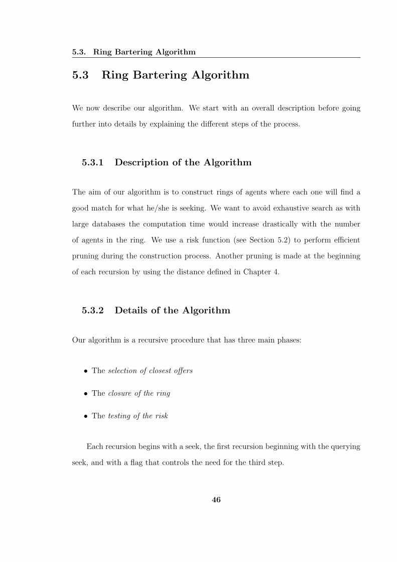
5.3.1 Description of the Algorithm

The aim of our algorithm is to construct rings of agents where each one will find a

good match for what he/she is seeking. We want to avoid exhaustive search as with

large databases the computation time would increase drastically with the number

of agents in the ring. We use a risk function (see Section 5.2) to perform efficient

pruning during the construction process. Another pruning is made at the beginning

of each recursion by using the distance defined in Chapter 4.

5.3.2 Details of the Algorithm

Our algorithm is a recursive procedure that has three main phases:

• The selection of closest offers

• The closure of the ring

• The testing of the risk

Each recursion begins with a seek, the first recursion beginning with the querying

seek, and with a flag that controls the need for the third step.

46

5.3. Ring Bartering Algorithm

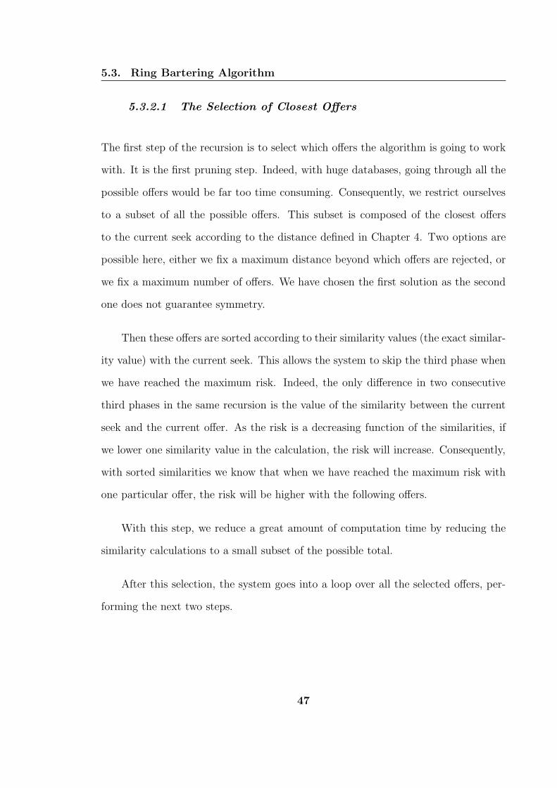
5.3.2.1 The Selection of Closest Offers

The first step of the recursion is to select which offers the algorithm is going to work

with. It is the first pruning step. Indeed, with huge databases, going through all the

possible offers would be far too time consuming. Consequently, we restrict ourselves

to a subset of all the possible offers. This subset is composed of the closest offers

to the current seek according to the distance defined in Chapter 4. Two options are

possible here, either we fix a maximum distance beyond which offers are rejected, or

we fix a maximum number of offers. We have chosen the first solution as the second

one does not guarantee symmetry.

Then these offers are sorted according to their similarity values (the exact similar-

ity value) with the current seek. This allows the system to skip the third phase when

we have reached the maximum risk. Indeed, the only difference in two consecutive

third phases in the same recursion is the value of the similarity between the current

seek and the current offer. As the risk is a decreasing function of the similarities, if

we lower one similarity value in the calculation, the risk will increase. Consequently,

with sorted similarities we know that when we have reached the maximum risk with

one particular offer, the risk will be higher with the following offers.

With this step, we reduce a great amount of computation time by reducing the

similarity calculations to a small subset of the possible total.

After this selection, the system goes into a loop over all the selected offers, per-

forming the next two steps.

47

5.3. Ring Bartering Algorithm

Figure 5.2: The Selection of Closest Offers

5.3.2.2 The Closure of the Ring

The second step of the recursion, the first of the loop, is to close the current ring. The

ring currently starts from the original seek and ends with the offer selected during

the previous step.

Thus to close the ring we need to get the similarity between the seek of the last

added agent and the offer of the very first agent in the ring. However, if we return

the ring like this, we lose the symmetry of the algorithm. Indeed, at every step, we

restrict the offers to those within the distance Dmax of the current seek. Consequently,

we must do the same here and test the distance between the last seek and the offer

of the first agent. If this distance is above Dmax, the ring must be rejected in order

to keep symmetry.

Finally, as we close the ring, we must compute the generalized aggregate simi-

larity and the final risk value to be reported to the user if it is below the maximum

authorized risk.

48

5.3. Ring Bartering Algorithm

Figure 5.3: The Closure of the Ring

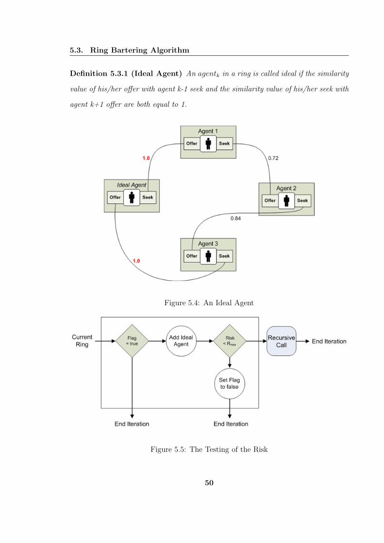
5.3.2.3 The Testing of the Risk

The last step of the loop is the most important. It tells whether the algorithm should

continue further in the recursion or not. This step is based on the risk function.

We calculate the risk of the current ring where we have added an ideal agent (see

Definition 5.3.1) and compare this value to Rmax.

If the risk is above the maximum value, we know that adding more agents to

the ring will leave the risk above this maximum. This results from Proposition 5.2.1.

Consequently, we do not need to go further. Moreover, as the offers selected in step

one are sorted according to their similarities, we don’t need to perform this test again

for this recursion. We thus inform the system by changing the value of the flag.

If the risk is below Rmax, we can create a ring with another agent that might

improve the generalized aggregate similarity of the whole ring while remaining below

the maximum risk. Consequently, we recursively call the procedure with the seek of

the last added agent.

49

5.3. Ring Bartering Algorithm

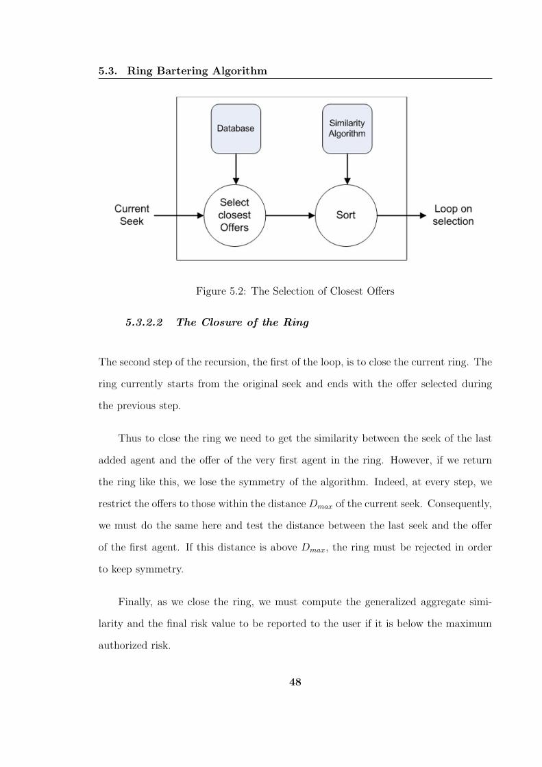
Definition 5.3.1 (Ideal Agent) An agentk in a ring is called ideal if the similarity

value of his/her offer with agent k-1 seek and the similarity value of his/her seek with

agent k+1 offer are both equal to 1.

Figure 5.4: An Ideal Agent

Figure 5.5: The Testing of the Risk

50

5.3. Ring Bartering Algorithm

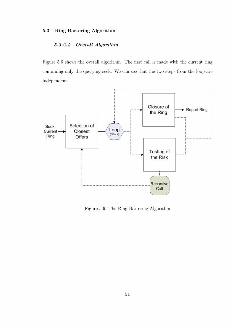
5.3.2.4 Overall Algorithm

Figure 5.6 shows the overall algorithm. The first call is made with the current ring

containing only the querying seek. We can see that the two steps from the loop are

independent.

Figure 5.6: The Ring Bartering Algorithm

51

5.3. Ring Bartering Algorithm

5.3.3 Properties of the Algorithm

Definition 5.3.2 (acceptable ring) A ring is called Dmax/Rmax acceptable if:

Condition 1. The distance between a seek and the offer of the next agent is below

Dmax.

Condition 2. The risk is below Rmax.

Our algorithm verifies the following soundness and completeness properties.

Property 5.3.1 (soundness) All rings reported by the algorithm are Dmax/Rmax

acceptable.

The proof of the first condition is immediate as we only consider offers that are

within a given distance. The second condition in order to be Dmax/Rmax acceptable

results directly from the testing during the closure phase.

Property 5.3.2 (completeness) All the rings starting from an Agentj of the agent

database that are Dmax/Rmax acceptable will be reported by the algorithm called with

Agentj as argument.

Proof: Let Rn be a ring of n agents that are Dmax/Rmax acceptable. From its first

condition, we know that if we start a recursion with the first k agents of Rn, the

(k + 1)-th agent’s offer will be selected in the first step of the recursion.

Now we have to show that the recursion will continue with the (k + 1)-th agent’s

seek. The pursuit of the recursion is dictated by the risk function. After having

52

5.3. Ring Bartering Algorithm

selected Offerk+1 an ideal agent is added to the ring and the risk is calculated.

However by hypothesis we know that the risk of Rn is below the maximum authorized

risk. Thus we know that the risk of a ring Rideal composed of the k + 1 first agent of

Rn and n− k− 1 ideal agents will be below Rmax, as the risk is a decreasing function

of the similarity values. Finally according to Proposition 5.2.1 we know that the risk

of the current ring with an ideal agent will be below the risk of Rideal and thus below

Rmax. Consequently the recursion will continue and the property is true.

Based on the two properties above we state the following theorem.

Theorem 5.3.1 A ring starting from an Agentj of the agent database will be reported

by the algorithm, called with Agentj as argument, if and only if it is Dmax/Rmax

acceptable.

Corollary 5.3.1 Suppose a ring is reported by the algorithm when starting with a

given agent. This ring, except for the labelling of the agents, will be also reported if

we start the algorithm with any of the other agents in the ring.

Proof: Let R be a ring reported by the algorithm starting with Agentj and j, k ∈

1..m where m is the number of agents in the database. This ring satisfies the two

conditions of Theorem 5.3.1. If we start the algorithm with an Agentk of R, all

rings that satisfy the conditions of Theorem 5.3.1 and which start with Agentk will

be reported. The ring R′ composed of all the agents of R in the same order but

starting with Agentk obviously shares the same risk value as R and has the same

set of similarity values between the consecutive offers and seeks. Consequently, R′

satisfies the conditions of Theorem 5.3.1 and will be reported.

53

5.4. Extended Algorithm for Bartering Tuples

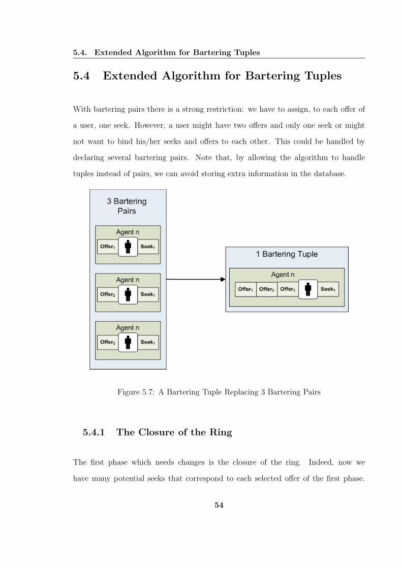
5.4 Extended Algorithm for Bartering Tuples

With bartering pairs there is a strong restriction: we have to assign, to each offer of

a user, one seek. However, a user might have two offers and only one seek or might

not want to bind his/her seeks and offers to each other. This could be handled by

declaring several bartering pairs. Note that, by allowing the algorithm to handle

tuples instead of pairs, we can avoid storing extra information in the database.

Figure 5.7: A Bartering Tuple Replacing 3 Bartering Pairs

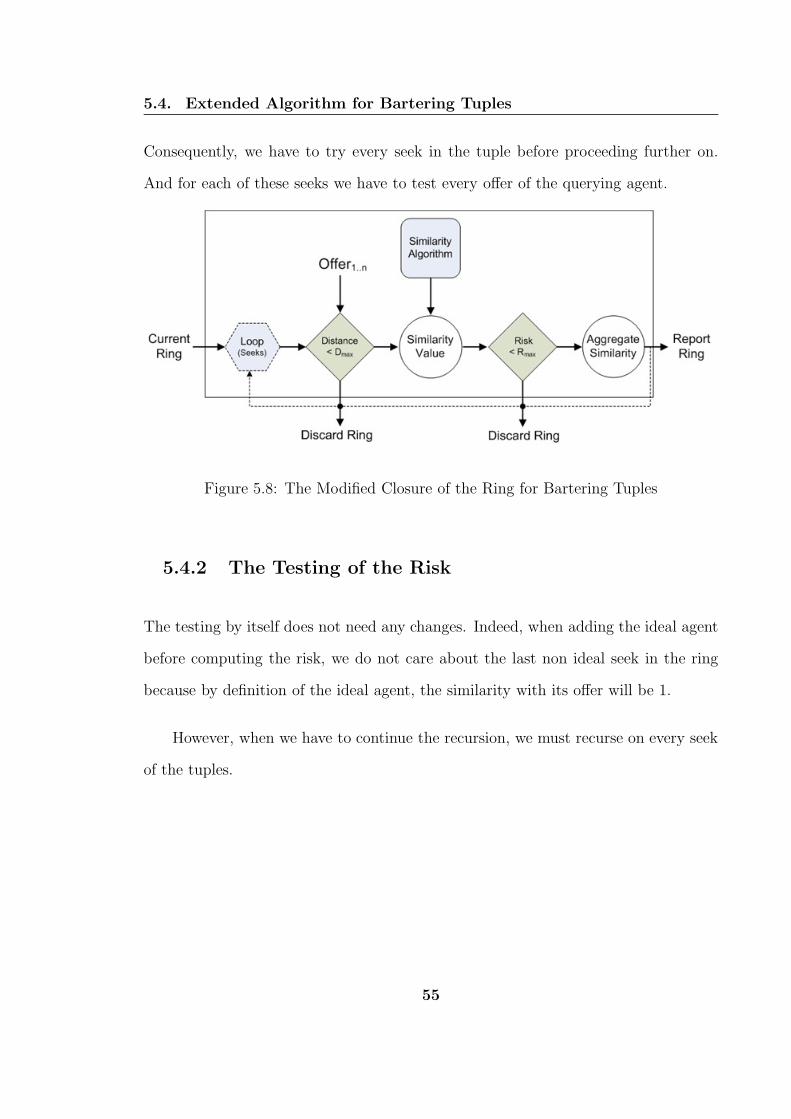
5.4.1 The Closure of the Ring

The first phase which needs changes is the closure of the ring. Indeed, now we

have many potential seeks that correspond to each selected offer of the first phase.

54

5.4. Extended Algorithm for Bartering Tuples

Consequently, we have to try every seek in the tuple before proceeding further on.

And for each of these seeks we have to test every offer of the querying agent.

Figure 5.8: The Modified Closure of the Ring for Bartering Tuples

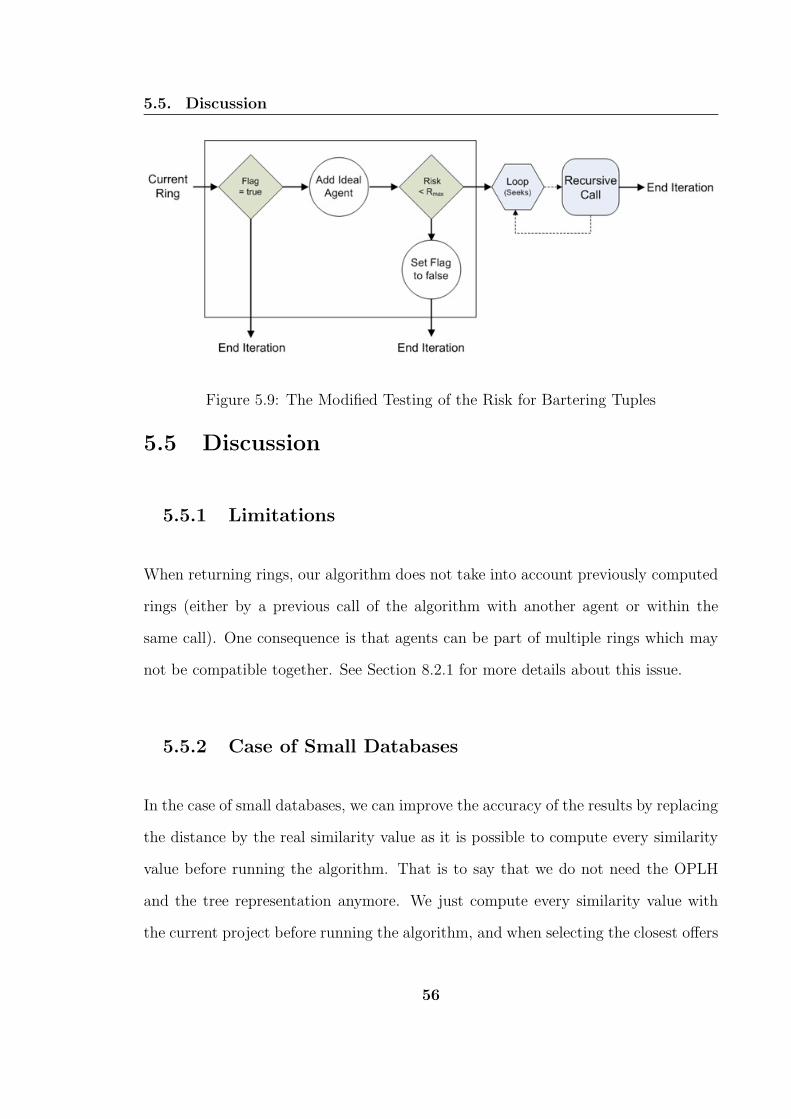
5.4.2 The Testing of the Risk

The testing by itself does not need any changes. Indeed, when adding the ideal agent

before computing the risk, we do not care about the last non ideal seek in the ring

because by definition of the ideal agent, the similarity with its offer will be 1.

However, when we have to continue the recursion, we must recurse on every seek

of the tuples.

55

5.5. Discussion

Figure 5.9: The Modified Testing of the Risk for Bartering Tuples

5.5 Discussion

5.5.1 Limitations

When returning rings, our algorithm does not take into account previously computed

rings (either by a previous call of the algorithm with another agent or within the

same call). One consequence is that agents can be part of multiple rings which may

not be compatible together. See Section 8.2.1 for more details about this issue.

5.5.2 Case of Small Databases

In the case of small databases, we can improve the accuracy of the results by replacing

the distance by the real similarity value as it is possible to compute every similarity

value before running the algorithm. That is to say that we do not need the OPLH

and the tree representation anymore. We just compute every similarity value with

the current project before running the algorithm, and when selecting the closest offers

56

5.5. Discussion

(resp. seek) to the current seek (resp. offer) we take the closest one according to the

similarity.

5.5.3 Storing similarity values

To avoid computing many times the same similarity values, the system has to store

them on the fly each time a new value is computed. Of course, in case of a modification

of a tree, these values have to be reset.

5.5.4 Bidirectional Search

In all previous sections, we have assumed that the starting point of our algorithm

is a seek. Instead, starting with an offer will not change the algorithm, we only

need to replace seek by offer, and conversely, everywhere in the algorithm. To allow

both, the system just has to remember from where the process has started and act

correspondingly. With the same kind of proof as for Theorem 5.3.1 we can show that

going from the offer direction will not provide different results.

Consequently, a bidirectional search, will not provide better results. One use

of bidirectional search could be to parallelize the computation by starting in both

directions at the same time. However, this would raise a problem as it would be

difficult to find a meeting point. One possible way to parallelize the algorithm would

be to wait for the first recursions to occur and distribute these recursions among the

processors/computers.

57

5.5. Discussion

5.5.5 Multiple calls

In all previous sections, we have always consider that our algorithm was focusing on

one particular agent. In order to get all possible Dmax/Rmax acceptable rings for a

given set of agents, the algorithm must be called with each agent as a starting point.

5.5.6 Complexity

The complexity of our algorithm is discussed in Section 7.3.

58

CHAPTER 6

An Application: Teclantic.ca

In order to test our system, we decided to implement it on the Teclantic.ca portal.

In this chapter we describe the portal before explaining some specifics and choices of

the implementation. The results of the testing are given in Chapter 7.

6.1 Description of Teclantic.ca

Teclantic.ca is a technology transfer portal for the research area in the Atlantic

Canadian region. The portal is using the AgentMatcher Tree similarity algorithm

[1, 5, 4, 32] to provide the user with the opportunity to contact other users having

similar projects. It is a match-making portal where the negotiation phase is left to

the user by means of an internal message service.

59

6.2. Details of Teclantic.ca for the Bartering System

One key difference to most other match-making portals is the weighting scheme

which allows the user to give more or less importance to the different partonomic and

taxonomic branches of his/her project.

Extending this portal to bartering and ring bartering will enhance further the

possibilities given to the user for facilitating collaborative work in the research area.

6.2 Details of Teclantic.ca for the Bartering Sys-

tem

In order to understand fully the next chapter, it is required that we review some

specifics of Teclantic.ca that have a direct influence on our algorithm.

6.2.1 Bartering Tuples

Teclantic.ca deals with research projects. Bartering pairs in the research area is not

really judicious. Indeed in most cases the following situations are going to occur:

• A user has only project offers ( e.g. a research group looking for funding ).

• A user has only projects seeks ( e.g. a venture capitalist seeking for technologies

).

• A user has both offers and seeks but not the same number of each.

Consequently, we have to implement a system that will deal with the two first

cases as well as the third one. The two first cases are easy to take care of. We only

60

6.2. Details of Teclantic.ca for the Bartering System

need to test whether the project has at least a corresponding offer (resp. seek) or not,

and run the actual similarity algorithm or the ring bartering algorithm accordingly.

The third case requires the use of the Extended Algorithm for Bartering Tuples (see

Section 5.4). Moreover, with this extended algorithm, every offer (resp. seek) of

a user can form a potential bartering pair with any seek (resp. offer) of this user.

We consequently remove the artificial binding between a user’s offers and seeks that

would be required with bartering pairs and which does not appear very meaningful

in the research area.

Finally, some projects may have an offer and a seek at the same time. Indeed

a research group may be willing to start a collaborative work with another group

working in the same area.

6.2.2 Tree Representation

In Teclantic.ca, the trees are separated in two parts. The first part has fixed arcs,

nodes and weights. Only the leaves are varying. It describes the general information

about the project. The weight of this subtree is 0.3. The second part is the description

of the areas of the project. The nodes and leaves are empty and the possible arc-labels

are from a given set. This subtree is a two-level tree, each level corresponding to a

level of the taxonomy (see Figure 6.1).

To represent these trees in a multi-dimensional space we are only going to focus

on the taxonomy part of the tree as we would need to go to the leaf level to get some

information on the general information part. Also we will restrict the base of trees

to one-level trees. As the taxonomy is quite important we would have far too many

dimensions with two-level trees. With one-level trees we already have 29 possible

61

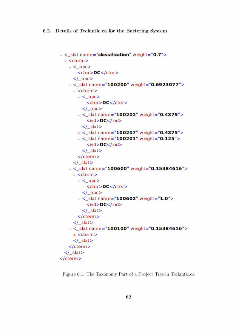
6.2. Details of Teclantic.ca for the Bartering System

Figure 6.1: The Taxonomy Part of a Project Tree in Teclantic.ca

62

6.2. Details of Teclantic.ca for the Bartering System

arc-labels and consequently 29 dimensions in our space. Figure 6.2 shows the values

of the corresponding 29 coordinates (x1 to x29) for a sample tree.

Figure 6.2: An example of Tree with its Representation

As we can see in the previous example, most of the coordinates are 0. This is

why we must not have too many dimensions in our space, as the splitting process

of linear hashing will never reach the last coordinates if the number of dimensions is

too high. Already with 29 it is not likely that a split on the last dimension will ever

occur. We are going to further explain this problem in the next section.

6.2.3 Order Preserving Linear Hashing

One peculiarity of the Teclantic.ca trees is that many of the coordinates of a tree in

the multi-dimensional space are going to be 0. Indeed it is not likely that a project

will be classified under more than two or three main taxonomy category items. With

such a small amount of data the division of space is only on the first few coordinates.

Consequently, many projects are going to be in the same bucket because these first

63

6.2. Details of Teclantic.ca for the Bartering System

Figure 6.3: The Repartitioning of the Trees in the Buckets

few coordinates are going to be null (see Figure 6.3). This will slow down the range

query process as the system will have to check many trees after retrieving them from

the buckets. In a worst case scenario, all the projects are going to be in the same

bucket and the range query function will have to check all of them to see if they are

within the querying distance. Nonetheless, this will still be faster than computing

every similarity value.

However, it is possible to artificially work around this problem by increasing the

number of buckets. Indeed we can start with an OPLH of high level which will allow

a better repartition in the buckets. Or, we can decrease the size of the buckets to

speed up the splitting process. Still, it will also slow down the range querying process

by forcing more and more intersection checks between subspaces and the query and

also more bucket retrievals.

Another solution, would be to perform a multiple OPLH. That is to say that,

instead of storing all points in bucket 0 as they are, we could re-hash them, starting

64

6.2. Details of Teclantic.ca for the Bartering System

from another coordinate, and store them in another OPLH. For example we have 29

dimensions in Teclantic: we could have 2 level 10 and one level 9 OPLH. It would

only increase the number of buckets by a factor of 3 instead of having 229 buckets if

we wanted to retain a single level 29 OPLH.

However, as long as Teclantic is not dealing with a great amount of data, we can

replace the distance by the real similarity value, as exposed in Section 5.5.2.

65

CHAPTER 7

Computational Results

We now present computational test results of our system. One must keep in mind

that the results are dependant on the kind of data we are dealing with. We will

first present some results on the influence of the distance, then we will discuss the

influence of the risk before showing the outcomes of computation time testings.

All the tests, except when mentioned otherwise, are done with 2- and 3-agent

rings.

7.1 Influence of the Distance

Two main aspects must be tested for the distance. First, the behavior of the distance

against the similarity. This is to justify our choice of distance. And secondly, the

66

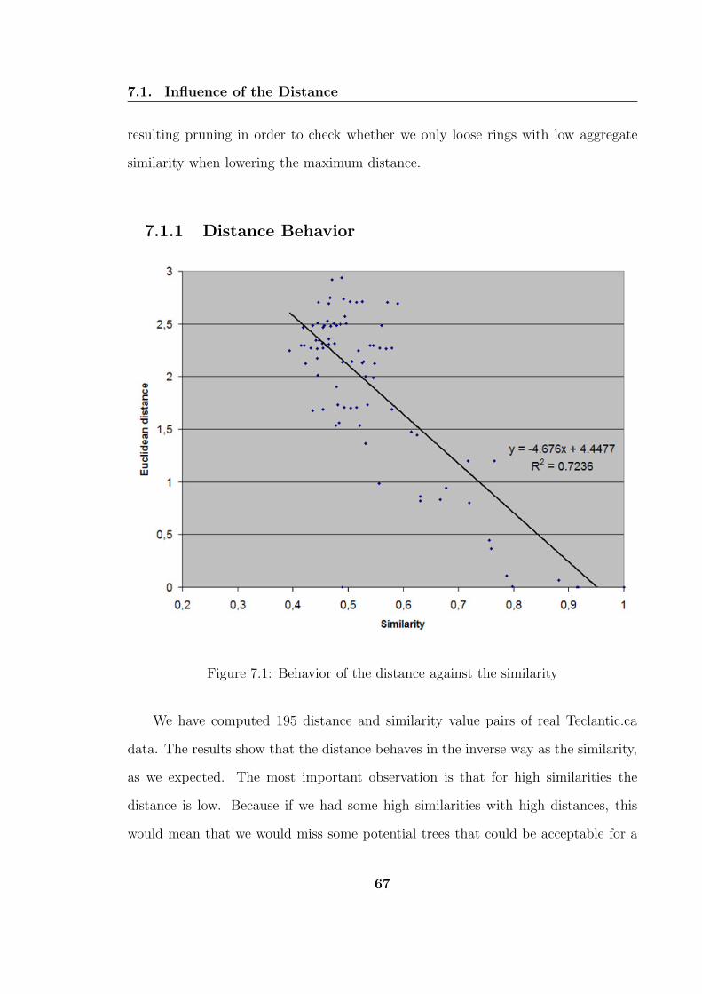
7.1. Influence of the Distance

resulting pruning in order to check whether we only loose rings with low aggregate

similarity when lowering the maximum distance.

7.1.1 Distance Behavior

Figure 7.1: Behavior of the distance against the similarity

We have computed 195 distance and similarity value pairs of real Teclantic.ca

data. The results show that the distance behaves in the inverse way as the similarity,

as we expected. The most important observation is that for high similarities the

distance is low. Because if we had some high similarities with high distances, this

would mean that we would miss some potential trees that could be acceptable for a

67

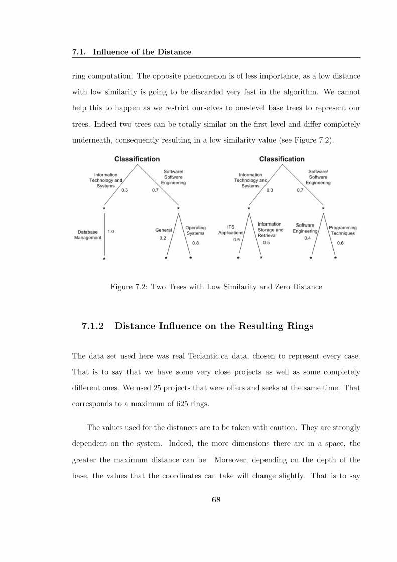
7.1. Influence of the Distance

ring computation. The opposite phenomenon is of less importance, as a low distance

with low similarity is going to be discarded very fast in the algorithm. We cannot

help this to happen as we restrict ourselves to one-level base trees to represent our

trees. Indeed two trees can be totally similar on the first level and differ completely

underneath, consequently resulting in a low similarity value (see Figure 7.2).

Figure 7.2: Two Trees with Low Similarity and Zero Distance

7.1.2 Distance Influence on the Resulting Rings

The data set used here was real Teclantic.ca data, chosen to represent every case.

That is to say that we have some very close projects as well as some completely

different ones. We used 25 projects that were offers and seeks at the same time. That

corresponds to a maximum of 625 rings.

The values used for the distances are to be taken with caution. They are strongly

dependent on the system. Indeed, the more dimensions there are in a space, the

greater the maximum distance can be. Moreover, depending on the depth of the

base, the values that the coordinates can take will change slightly. That is to say

68

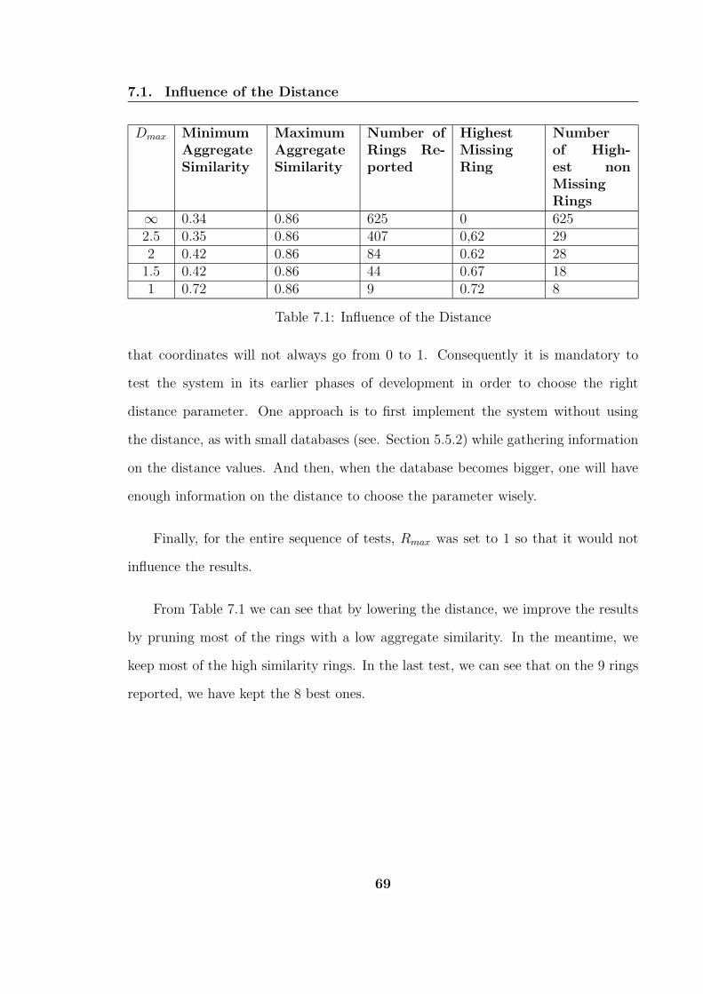
7.1. Influence of the Distance

Dmax MinimumAggregateSimilarity

MaximumAggregateSimilarity

Number ofRings Re-ported

HighestMissingRing

Numberof High-est nonMissingRings

∞ 0.34 0.86 625 0 6252.5 0.35 0.86 407 0,62 292 0.42 0.86 84 0.62 28

1.5 0.42 0.86 44 0.67 181 0.72 0.86 9 0.72 8

Table 7.1: Influence of the Distance

that coordinates will not always go from 0 to 1. Consequently it is mandatory to

test the system in its earlier phases of development in order to choose the right

distance parameter. One approach is to first implement the system without using

the distance, as with small databases (see. Section 5.5.2) while gathering information

on the distance values. And then, when the database becomes bigger, one will have

enough information on the distance to choose the parameter wisely.

Finally, for the entire sequence of tests, Rmax was set to 1 so that it would not

influence the results.

From Table 7.1 we can see that by lowering the distance, we improve the results

by pruning most of the rings with a low aggregate similarity. In the meantime, we

keep most of the high similarity rings. In the last test, we can see that on the 9 rings

reported, we have kept the 8 best ones.

69

7.2. Risk Influence on the Resulting Rings

Rmax MinimumAggregateSimilarity

MaximumAggregateSimilarity

Number ofRings Re-ported

HighestMissingRing

Numberof High-est nonMissingRings

1 0.34 0.86 625 0 6250.9 0.34 0.86 625 0 6250.8 0.34 0.86 625 0 6250.7 0.34 0.86 501 0.44 3970.6 0.4 0.86 93 0.57 740.5 0.52 0.86 18 0.69 130.4 0.65 0.86 6 0.78 40.3 0.72 0.85 3 0.86 00.2 0.84 0.85 2 0.86 00.1 0 0 0 0.86 00 0 0 0 0.86 0

Table 7.2: Influence of the Risk on Teclantic.ca Data

7.2 Risk Influence on the Resulting Rings

We performed here two series of tests. One with the same data set as in the previous

section. The other with random similarity values. It was not relevant to perform the

previous tests on the distance with random similarity values. Indeed, the distance

is linked with the similarity but is not the result of a computation implying the

similarity values. If we had used random similarity values in the previous section,

we would have lost the correlation between the distance and the similarity. On the

contrary, the risk is directly computed from the similarity values and having random

data will not change the correlation. For both tests, Dmax was set to ∞ so that it

would not interfere with the results.

Most of the results in Tables 7.2 and 7.3 are satisfactory. The pruning is mostly

done on the bottom aggregate similarity values and we keep most of the top rings,

even with low risk values. In both cases, from a risk of 0.3 we loose the best ring

70

7.3. Computation Times

Rmax MinimumAggregateSimilarity

MaximumAggregateSimilarity

Number ofRings Re-ported

HighestMissingRing

Numberof High-est nonMissingRings

1 0.02 0.89 625 0 6250.9 0.11 0.89 499 0.47 2480.8 0.21 0.89 372 0.5 2160.7 0.38 0.89 225 0.55 1640.6 0.43 0.89 134 0.62 1040.5 0.51 0.89 42 0.7 340.4 0.61 0.89 11 0.81 70.3 0.71 0.89 6 0.88 20.2 0.82 0.89 5 0.88 20.1 0 0 0 0.89 00 0 0 0 0.89 0

Table 7.3: Influence of the Risk with Random Similarity Values

(according to the aggregate similarity). This is not alarming. Indeed the risk value

reflects more the low similarities in the ring than the aggregate similarity. That is

to say that if a similarity value is low and the others high, the risk will be more

influenced than the aggregate similarity.

7.3 Computation Times

7.3.1 Theoretical Results

Giving an exact time complexity for our algorithm is not an easy task. Indeed as the

computation time depends on the repartition of the data (i.e. the different similarity

values), Dmax and Rmax it is hardly possible to provide a general formula. However

we can still give some information on the algorithm’s behavior.

71

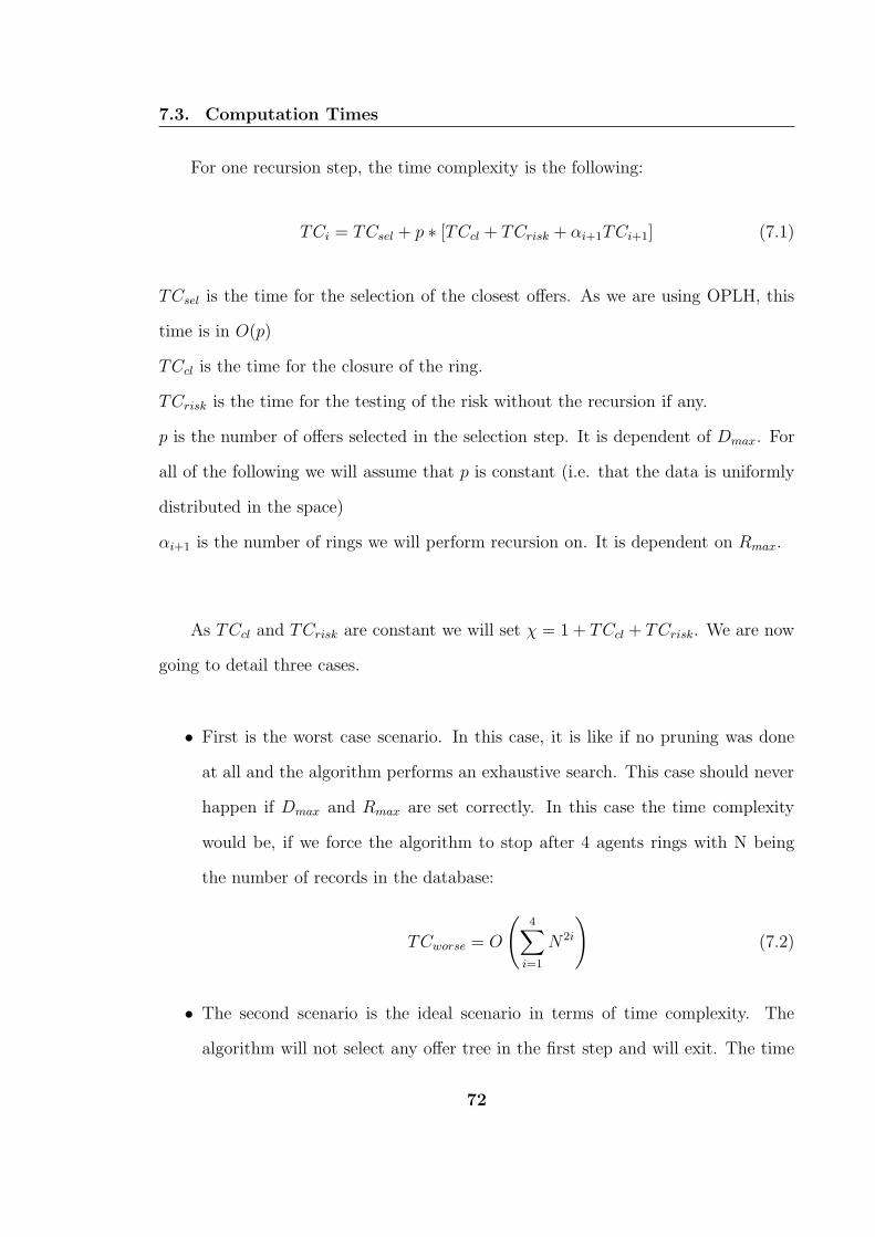
7.3. Computation Times

For one recursion step, the time complexity is the following:

TCi = TCsel + p ∗ [TCcl + TCrisk + αi+1TCi+1] (7.1)

TCsel is the time for the selection of the closest offers. As we are using OPLH, this

time is in O(p)

TCcl is the time for the closure of the ring.

TCrisk is the time for the testing of the risk without the recursion if any.

p is the number of offers selected in the selection step. It is dependent of Dmax. For

all of the following we will assume that p is constant (i.e. that the data is uniformly

distributed in the space)

αi+1 is the number of rings we will perform recursion on. It is dependent on Rmax.

As TCcl and TCrisk are constant we will set χ = 1 + TCcl + TCrisk. We are now

going to detail three cases.

• First is the worst case scenario. In this case, it is like if no pruning was done

at all and the algorithm performs an exhaustive search. This case should never

happen if Dmax and Rmax are set correctly. In this case the time complexity

would be, if we force the algorithm to stop after 4 agents rings with N being

the number of records in the database:

TCworse = O

(

4∑

i=1

N2i

)

(7.2)

• The second scenario is the ideal scenario in terms of time complexity. The

algorithm will not select any offer tree in the first step and will exit. The time

72

7.3. Computation Times

complexity is obviously in O(1).

• Finally for a more general scenario we will start from Equation ( 7.1) with i = 0

and will find a global formula by induction.

TC0 = TCsel + p ∗ [TCcl + TCrisk + α1TC1]

= O (p + p ∗ [χ − 1 + α1TC1])

= O (p · χ + p · α1TC1)

= O (p · χ + p · α1 · [p · χ + p · α2TC2])

= O (p · χ + p2 · α1χ + p2 · α1α2TC2)

= O (p · χ + p2 · α1χ + p2 · α1α2 · [p · χ + p · α3TC3])

= O (p · χ + p2 · α1χ + p3 · α1α2χ + p3 · α1α2α3TC3)

= ...

(7.3)

From this we can show by induction that the general result is the following, α∞

being equal to 0:

TC = O

(

∞∑

i=1

(

pi · Πi−1

k=1αk

)

)

(7.4)

Of course in practise, as shown in Table 7.5, from i = 7 all αi will be null. With

well parameterized Rmax it will probably be from i = 5.

If we want a formula depending on N , we have to express p as a percentage of

N and make some hypothesis on the αi. We will assume that p is 1% of N .

Then we will assume that α1 is 90% of p and that we divide the amount by 2

every time we increase i. And from i = 5 we will assume that the algorithm

will not perform any more recursion.

73

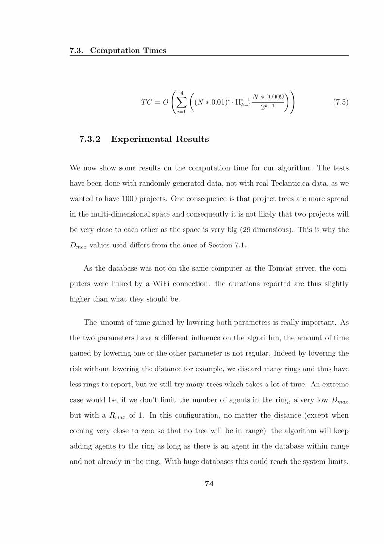
7.3. Computation Times

TC = O

(

4∑

i=1

(

(N ∗ 0.01)i · Πi−1

k=1

N ∗ 0.009

2k−1

)

)

(7.5)

7.3.2 Experimental Results

We now show some results on the computation time for our algorithm. The tests

have been done with randomly generated data, not with real Teclantic.ca data, as we

wanted to have 1000 projects. One consequence is that project trees are more spread

in the multi-dimensional space and consequently it is not likely that two projects will

be very close to each other as the space is very big (29 dimensions). This is why the

Dmax values used differs from the ones of Section 7.1.

As the database was not on the same computer as the Tomcat server, the com-

puters were linked by a WiFi connection: the durations reported are thus slightly

higher than what they should be.

The amount of time gained by lowering both parameters is really important. As

the two parameters have a different influence on the algorithm, the amount of time

gained by lowering one or the other parameter is not regular. Indeed by lowering the

risk without lowering the distance for example, we discard many rings and thus have

less rings to report, but we still try many trees which takes a lot of time. An extreme

case would be, if we don’t limit the number of agents in the ring, a very low Dmax

but with a Rmax of 1. In this configuration, no matter the distance (except when

coming very close to zero so that no tree will be in range), the algorithm will keep

adding agents to the ring as long as there is an agent in the database within range

and not already in the ring. With huge databases this could reach the system limits.

74

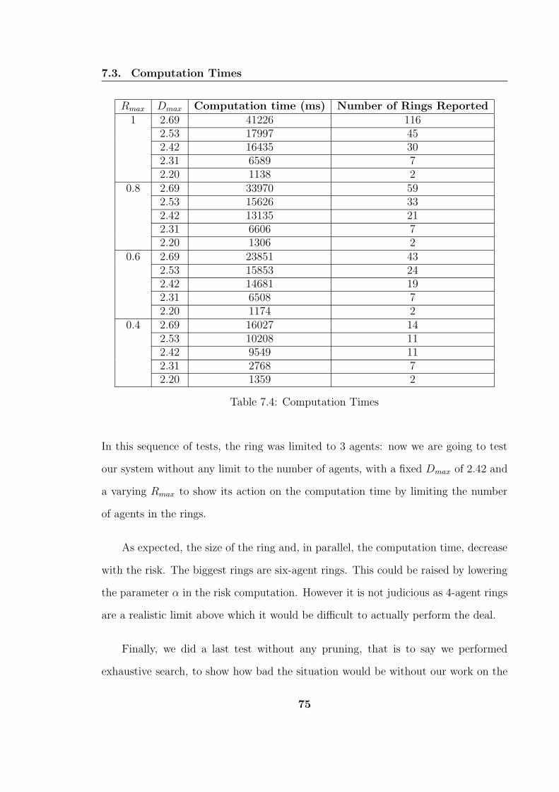
7.3. Computation Times

Rmax Dmax Computation time (ms) Number of Rings Reported1 2.69 41226 116

2.53 17997 452.42 16435 302.31 6589 72.20 1138 2

0.8 2.69 33970 592.53 15626 332.42 13135 212.31 6606 72.20 1306 2

0.6 2.69 23851 432.53 15853 242.42 14681 192.31 6508 72.20 1174 2

0.4 2.69 16027 142.53 10208 112.42 9549 112.31 2768 72.20 1359 2

Table 7.4: Computation Times

In this sequence of tests, the ring was limited to 3 agents: now we are going to test

our system without any limit to the number of agents, with a fixed Dmax of 2.42 and

a varying Rmax to show its action on the computation time by limiting the number

of agents in the rings.

As expected, the size of the ring and, in parallel, the computation time, decrease

with the risk. The biggest rings are six-agent rings. This could be raised by lowering

the parameter α in the risk computation. However it is not judicious as 4-agent rings

are a realistic limit above which it would be difficult to actually perform the deal.

Finally, we did a last test without any pruning, that is to say we performed

exhaustive search, to show how bad the situation would be without our work on the

75

7.3. Computation Times

Rmax Computation time(ms)

Number of RingsReported

Biggest Ring

0.9 54972 67 60.8 38887 42 50.7 33601 32 40.6 22311 21 40.5 15540 15 30.4 9064 11 30.3 1576 5 2

Table 7.5: Computation Times and Size of the Rings

Maximum authorized size of theRing

Computation time (ms)

2 5383 32524 415205 249973

Table 7.6: Computation Times without Pruning

risk and the distance. We worked with only 10 projects (which were offers and seeks

at the same time). Table 7.6 shows the results. When the size of the ring is increased,

the computation time becomes really bad very fast, and this with very few projects

to work with. This gives us the confirmation of what we had stated at the beginning

and justifies our work on this problem.

76

CHAPTER 8

Conclusion

8.1 Contributions

We have presented an algorithm to extend the usual buyer/seller scenario to, first,

bartering and, then, to ring bartering allowing several agents to take part in the same

trade. By representing the weighted trees in a multi-dimensional space, we allowed

an efficient pruning to be done in the early phase of our algorithm by using the notion

of distance instead of the similarity. Then we introduced the risk to limit the ring

construction process and to restrain the results to viable rings.

• The buyer/seller scenario, even if widespread among web portals, finds its limits

when dealing, for example, with knowledge that is difficult to quantify with

money. Bilateral bartering allows to handle naturally and easily any kind of

77

8.1. Contributions

“goods”. To rate a potential deal, we introduced the aggregate similarity value

of two pairs of trees. By using the weighted tree similarity algorithm we allow

user to specify detailed queries both on the offering and the seeking side.

• By definition the buyer/seller scenario is a two sided deal. Shifting to barter-

ing allows more sides to be part of the same trade thus increasing the global

satisfaction of each party. We developed a ring bartering algorithm which gives

the user 2- to n-agent deals. These rings are rated according to a naturally

generalized aggregate similarity value.

• As we allow n-agents deals, we developed two pruning techniques to avoid ex-

haustive search which would cause drastic performance losses.

We first used an approximate representation of the weighted trees in a multi-

dimensional space and defined the distance between two trees in this space.

Thanks to certain efficient data-structures such as the OPLH we can perform

efficient pruning in the first phase of our algorithm by testing only the trees

closest to the current one.

Then, we introduced the risk of a ring which is a measure of how likely the deal

is not going to happen. This value based on the number of agents as well as

the similarity values of the ring allows a second pruning phase and prevents the

algorithm from adding agents infinitely.

Finally, we proved Theorem 5.3.1 and its Corollary to verify the correctness of

our algorithm.

78

8.2. Future Work

8.2 Future Work

8.2.1 Pairing

One major area in continuation of our work is the pairing problem. Currently our

algorithm returns rings regardless of the availability of the agents involved. That is to

say that an agent can be involved in many rings. Of course this agent will not be able

to perform all the deals where his/her name appears. Consequently, the natural next

step to our system would be a pairing algorithm that would try to create the best

combination of rings implying every agent in the virtual market place so that everyone

would be part of exactly one deal. For this another measure would be needed, an

equivalent to the aggregate similarity but for the entire market place. And the system

would have to maximize this value. As this problem is close to the traveling salesman

problem, the time complexity for an exact solution will probably be very high and an

approximate algorithm would probably be needed to make it practical.

8.2.2 Local Similarity

As mentioned in section 4.2.3, the use of local similarity measures on nodes and leaves,

as developed in [4], can greatly improve our tree representation in a multi-dimensional

space. For example, in our Teclantic.ca portal we could add the general information

part of the tree without adding too much dimensions.

79

References

[1] Agentmatcher group website. http://www.cs.unb.ca/agentmatcher/.

[2] Ultralingua v5.0.3. http://www.ultralingua.com.

[3] T. Ackemann, R. Gold, C. Mascolo, and W. Emmerich. Incentives in Peer-to-Peer and Grid Networking. UCL Research Note RN/02/24, 2002.

[4] V.C. Bhavsar, H. Boley, and L. Yang M.Ball. Weighted Partonomy-TaxonomyTrees with Local Similarity Measures for Semantic Buyer-Seller Match-Making.In Proceedings of Workshop of Business Agents and the Semantic Web(BASeWEB’05), 8 May 2005.

[5] V.C. Bhavsar, H. Boley, and L. Yang. A Weighted Tree Similarity Algorithm forMulti-Agent System in E-Business Environments. Workshop on Business Agentsand the Semantic Web, pages 53–72, June 2003.

[6] H. Boley. Object-Oriented RuleML: User-level roles, URI-grounded clauses andorder-sorted terms. pages 1–16. Springer-Verlag, Heidelberg, LNCS-2876, 2003.

[7] S. Brin. Near Neighbor Search in Large Metric Spaces. The VLDB Journal,pages 574–584, 1995.

[8] A. Chavez and P. Maes. Kasbah: An Agent Marketplace for Buying and SellingGoods. In First International Conference on the Practical Application of Intelli-gent Agents and Multi-Agent Technology (PAAM’96), pages 75–90, London, UK,1996. Practical Application Company.

80

References

[9] B. Cresti. U.S. Domestic Barter: An Empirical Investigation. In TechnicalReport N.2003-5. Institut de Recherches Economiques et Sociales (IRES), 2003.

[10] W. Li E. Hiser, B. Lanka and F. Oliver. History of E-Commerce.http://newmedia.medill.northwestern.edu/courses/nmpspring01/brown/

Revstream/history.htm.

[11] H. Boley, V. C. Bhavsar, D. Hirtle, A. Singh, Z. Sun, and L. Yang. A match-making System for Learners and Learning Objects. In International Journal ofInteractive Technology and Smart Education, 2(3), pages 171–178, August 2005.online journal.

[12] P. Haddawy and C. Cheng. Balanced Matching of Buyers and Sellers in E-Marketplaces: The Barter Trade Exchange Model. December 2003. http://

citeseer.ist.psu.edu/haddawy03balanced.html.

[13] M. Han. History of E-Commerce : in the Context of Security Industry, 1999.

[14] A. Hutflesz, H.W. Six, and P. Widmayer. Globally Order Preserving Multidimen-sional Linear Hashing. In Proceedings of the Fourth International Conference onData Engineering, pages 572–579, Washington, DC, USA, 1988. IEEE ComputerSociety.

[15] N. Karacapilidis and P. Moraitis. Building an Agent-Mediated Electronic Com-merce System with Decision Analysis Features. Decision Support SyStems, 32,pages 53–69, 2001.

[16] H.P. Kriegel and B. Seeger. Multidimensional Order Preserving Linear Hashingwith Partial Expansions. In Proceedings on International conference on databasetheory, pages 203–220, New York, NY, USA, 1986. Springer-Verlag New York,Inc.

[17] P. Larson. A Single-File Version of Linear Hashing with Partial Expansions. InEigth International Conference on Very Large Data Bases, September 8-10, 1982,Mexico City, Mexico, Proceedings, pages 300–309. Morgan Kaufmann, 1982.

[18] W. Litwin. Linear Hashing: A New Tool for File and Table Addressing. Readingsin database systems (2nd ed.), pages 96–107, 1994.

[19] T.D. Noia, E.D. Sciascio, F.M. Donini, and M. Mongiello. Semantic Matchmak-ing in a P-2-P Electronic Marketplace. In SAC ’03: Proceedings of the 2003ACM symposium on Applied computing, pages 582–586, New York, NY, USA,2003. ACM Press.

81

References

[20] S. Onta and E. Plaza. A Bartering Approach to Improve Multiagent Learning.In AAMAS ’02: Proceedings of the first international joint conference on Au-tonomous agents and multiagent systems, pages 386–393, New York, NY, USA,2002. ACM Press.

[21] E.J. Otoo. A Multidimensional Digital Hashing Scheme for Files with CompositeKeys. In SIGMOD ’85: Proceedings of the 1985 ACM SIGMOD internationalconference on Management of data, pages 214–229, New York, NY, USA, 1985.ACM Press.

[22] M. Ouksel and P. Scheuermann. Storage Mappings for Multidimensional Lin-ear Dynamic Hashing. In PODS ’83: Proceedings of the 2nd ACM SIGACT-SIGMOD symposium on Principles of database systems, pages 90–105, New York,NY, USA, 1983. ACM Press.

[23] P. Pu and B. Faltings. Enriching buyers’ Experiences: the SmartClient Ap-proach. In CHI ’00: Proceedings of the SIGCHI conference on Human factors incomputing systems, pages 289–296, New York, NY, USA, 2000. ACM Press.

[24] J.T. Robinson. Order Preserving Linear Hashing Using Dynamic Key Statistics.In PODS ’86: Proceedings of the fifth ACM SIGACT-SIGMOD symposium onPrinciples of database systems, pages 91–99, New York, NY, USA, 1986. ACMPress.

[25] A. Ghorbani S. Marsh and V.C. Bhavsar. The ACORN Multi-Agent System.Web Intelligence and Agent Systems, pages 1–21, 2003.

[26] H. Samet. Hierarchical Representations of Point Data. Self-Published, 1998.

[27] G. Seyfang. Bartering for a Better Future ? Community Currencies and Sustain-able Consumption. University of East Anglia, Norwich, NR4 7TJ, UK. CSERGEWorking Paper EDM 94-10.

[28] J.H. Stout. The History of Bartering and Money. In Personal and Business Bar-tering, 1985. http://www.theorderoftime.com/politics/cemetery/stout/

h/pbb-24.htm.

[29] D. Veit, J.P. Muller, M. Schneider, and B. Fiehn. Matchmaking for AutonomousAgents in Electronic Marketplaces. In AGENTS ’01: Proceedings of the fifthinternational conference on Autonomous agents, pages 65–66, New York, NY,USA, 2001. ACM Press.

[30] H. Wang, S. Liao, and L. Liao. Modeling Constraint-Based Negotiating Agents.Decis. Support Syst. 33(2), pages 201–217, 2002.

82

References

[31] L. Yang. Weighted-Tree Similarity Techniques for Multi-Agent Systems. MCSthesis proposal, Faculty of Computer Science, University of New Brunswick, June2003.

[32] L. Yang, B.K. Sarker, V.C. Bhavsar, and H.Boley. A Weighted-Tree SimplicityAlgorithm for Similarity Matching of Partial Product Descriptions. In Proceed-ings of ISCA 14th International Conference on Intelligent and Adaptive Systemsand Software Engineering, pages 55–60, 20-22 July 2005.

83

APPENDIX A

Teclantic Data Sample

The following XML tree is a RuleML Object Oriented representation of the Agent-

Matcher project in the Teclantic.ca portal.

<cterm >

<_opc>

<ctor >Project </ctor >

</_opc>

<_slot name="title " weight ="0.05">

<ind >AgentMatcher</ind >

</_slot >

<_slot name="bSeek " weight ="0.0">

<ind >2</ind >

</_slot >

<_slot name="numpeople" weight ="0.05">

<ind >6</ind >

</_slot >

<_slot name="namepeople" weight ="0.0">

<ind />

</_slot >

<_slot name="website" weight ="0.05">

<ind >http: // agentmatcher.cs.unb .ca</ind >

</_slot >

<_slot name="copyright" weight ="0.0">

<ind />

</_slot >

<_slot name="description" weight ="0.05">

<ind >The AgentMatcher project is a project to develop a set of tools

used in creating systems used for comparison . The main sub

84

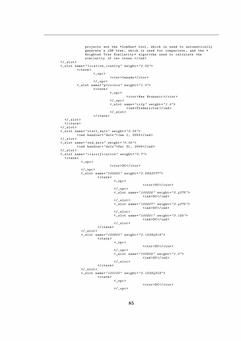
projects are the *LomGen * tool , which is used to automatically

generate a LOM tree , which is used for comparison , and the *

Weighted Tree Similarity * algorithm used to calculate the

similarity of two trees.</ind >

</_slot >

<_slot name="location_country" weight ="0.05">

<cterm >

<_opc >

<ctor>Canada </ctor >

</_opc>

<_slot name=" province" weight ="1.0">

<cterm >

<_opc>

<ctor>New Brunswic </ctor >

</_opc >

<_slot name="city" weight ="1.0">

<ind >Fredericton </ind >

</_slot >

</cterm >

</_slot >

</cterm >

</_slot >

<_slot name="start_date" weight ="0.05">

<ind handler ="date">Jan 1, 2003 </ind >

</_slot >

<_slot name="end_date" weight ="0.05">

<ind handler ="date">Dec 31, 2004</ind >

</_slot >

<_slot name="classification" weight ="0.7">

<cterm >

<_opc >

<ctor>DC</ctor>

</_opc >

<_slot name="100200 " weight =" 0.6923077">

<cterm >

<_opc>

<ctor >DC</ctor >

</_opc>

<_slot name="100202 " weight ="0.4375 ">

<ind >DC</ind >

</_slot >

<_slot name="100207 " weight ="0.4375 ">

<ind >DC</ind >

</_slot >

<_slot name="100201 " weight ="0.125">

<ind >DC</ind >

</_slot >

</cterm >

</_slot >

<_slot name="100600 " weight =" 0.15384616">

<cterm >

<_opc>

<ctor >DC</ctor >

</_opc>

<_slot name="100602 " weight ="1.0">

<ind >DC</ind >

</_slot >

</cterm >

</_slot >

<_slot name="100100 " weight =" 0.15384616">

<cterm >

<_opc>

<ctor >DC</ctor >

</_opc>

85

<_slot name="100108 " weight ="1.0">

<ind >DC</ind >

</_slot >

</cterm >

</_slot >

</cterm >

</_slot >

</cterm >

86

VITA

Candidate’s full name: Sebastien Stephen Pierre Mathieu

Place and date of birth: Reims, FranceMarch 05, 1983

Universities: 2002 - 2005Ecole nationale superieure des MinesSaint-Etienne, France

2004 - 2005University of New BrunswickFredericton, Canada