Embed Size (px)
Citation preview

MASTRAF: A DECENTRALIZED MULTI-AGENT SYSTEM FOR
NETWORK-WIDE TRAFFIC SIGNAL CONTROL WITH
DYNAMIC COORDINATION
BY
JUAN C MEDINA
DISSERTATION
Submitted in partial fulfillment of the requirements
for the degree of Doctor of Philosophy in Civil Engineering
in the Graduate College of the
University of Illinois at Urbana-Champaign, 2013
Urbana, Illinois
Doctoral Committee:
Professor Rahim F. Benekohal, Chair
Associate Professor Yanfeng Ouyang
Assistant Professor Daniel B. Work
Professor Gul Agha

ii
ABSTRACT
Continuous increases in traffic volume and limited available capacity in the roadway system
have created a need for improved traffic control. From traditional pre-timed isolated signals to
actuated and coordinated corridors, traffic control for urban networks has evolved into more
complex adaptive signal control systems. However, unexpected traffic fluctuations, rapid
changes in traffic demands, oversaturation, the occurrence of incidents, and adverse weather
conditions, among others, significantly impact the traffic network operation in ways that current
control systems cannot always cope with.
On the other hand, strategies for traffic control based on developments from the field of
machine learning can provide promising alternative solutions, particularly those that make use of
unsupervised learning such as reinforcement learning (RL) - also referred as approximate
dynamic programming (ADP) in some research communities. For the traffic control problem,
examples of convenient RL algorithms are the off-policy Q-learning and the ADP using a post
decision state variable, since they address processes with sequential decision making, do not
need to compute transition probabilities, and are well suited for high dimensional spaces.
A series of benefits are expected from these algorithms in the traffic control domain: 1)
no need of prediction models to transition traffic over time and estimate the best actions; 2)
availability of cost-to-go estimates at any time (appropriate for real-time applications); 3) self-
evolving policies; and 4) flexibility to make use of new sources of information part of emergent
Intelligent Transportation Systems (ITS) such as mobile vehicle detectors (Bluetooth and GPS
vehicle locators).
Given the potential benefits of these strategies, this research proposes MASTraf: a
decentralized Multi-Agent System for network-wide Traffic signal control with dynamic
coordination. MASTraf is designed to capture the behavior of the environment and take
decisions based on situations directly observed by RL agents. Also, agents can communicate
with each other, exploring the effects of temporary coalitions or subgroups of intersections as a
mechanism for coordination.

iii
Separate MASTraf implementations with similar state and reward functions using Q-
learning and ADP were tested using a microscopic traffic simulator (VISSIM) and real-time
manipulation of the traffic signals through the software’s COM interface. Testing was conducted
to determine the performance of the agents in scenarios with increasing complexity, from a
single intersection, to arterials and networks, both in undersaturated and oversaturated
conditions.
Results show that the multi-agent system provided by MASTraf improves its
performance as the agents accumulate experience, and the system was able to efficiently manage
the traffic signals of simple and complex scenarios. Exploration of the policies generated by
MASTraf showed that the agents followed expected behavior by providing green to greater
vehicle demands and accounting for the effects of blockages and lost time. The performance of
MASTraf was on par with current state of practice tools for finding signal control settings, but
MASTraf can also adapt to changes in demands and driver behavior by adjusting the signal
timings in real-time, thus improving coordination and preventing queue spillbacks and green
starvation.
A strategy for signal coordination was also tested in one of the MASTraf
implementations, showing increased throughput and reduced number of stops, as expected. The
coordination employed a version of the max-plus algorithm embedded in the reward structure,
acting as a bias towards improved coordination. The response of the system using imprecise
detector data, in the form of coarse aggregation, showed that the system was able to handle
oversaturation under such conditions. Even when the data had only 25% of the resolution of the
original implementation, the system throughput was only reduced by 5% and the number of stops
per vehicle was increased by 8%.
The state and reward formulations allowed for a simple function approximation method
in order to reduce the memory requirements for storing the state space, and also to create a form
of generalization for states that have not been visited or that have not been experienced enough.
Given the discontinuities in the reward function generated by penalties for blockages and lost
times, the value approximation was conducted through a series of functions for each action and
each of the conditions before and after a discontinuity.
The policies generated using MASTraf with a function approximation were analyzed for
different intersections in the network, showing agent behavior that reflected the principles

iv
formulated in the original problem using lookup tables, including right of way assignment based
on expected rewards with consideration of penalties such as lost time. In terms of system
performance, MASTraf with function approximation resulted in average reductions of 1% in the
total system throughput and 3.6% increases in the number of stops per vehicle, when compared
to the implementation using lookup tables on a congested network of 20 intersections.

v
ACKNOWLEDGEMENTS
I would like to specially thank my advisor Dr. Rahim F. Benekohal for his continuous support
and guidance, not only for the completion of this work, but throughout my graduate studies. I
would also like to thank Dr. Benekohal for the education received in the transportation program,
and for the practical, real-world experience acquired from a wide variety of projects I had the
opportunity to be part of.
I have met a great number of people over the last years. To them, I owe all the small and
big things that made my stay a truly great life experience; I am and I will always be truly grateful
for that. I finish the program with the best friends and peers, and hoping to keep in contact with
them for years to come.
Lastly, I would like to thank my parents for their unconditional support and constant
motivation. I am sure they appreciate this achievement as much as I do, and this it to them.

vi
TABLE OF CONTENTS
CHAPTER 1 - INTRODUCTION .................................................................................................. 1
1.1. MASTraf ............................................................................................................................... 4
CHAPTER 2 – LITERATURE REVIEW ...................................................................................... 8
2.1. Evolution of Traffic Control and Current Systems .............................................................. 8
2.2. Reinforcement Learning and Approximate Dynamic Programming over Time ................ 13
2.3. Traffic Control Using Learning Agents .............................................................................. 15
CHAPTER 3 – REVIEW OF REINFORCEMENT LEARNING AND APPROXIMATE
DYNAMIC PROGRAMMING .................................................................................................... 21
3.1. Fundamentals ...................................................................................................................... 21
3.2. Q-learning ........................................................................................................................... 24
3.3. The ADP with Post-decision State Variable....................................................................... 26
3.4. Eligibility Traces – a Bridge between Single-step Updates and Monte-Carlo ................... 29
CHAPTER 4 – PROPOSED MULTI-AGENT SYSTEM ........................................................... 31
4.1. Operational Description ...................................................................................................... 31
4.2. Implementation ................................................................................................................... 33
4.3. System Components ........................................................................................................... 34
CHAPTER 5 – EVALUATION OF MASTRAF IN TRAFFIC SIGNAL SYSTEMS ................ 41
5.1. Single Intersection - Oversaturated Conditions .................................................................. 41
5.2. Four-intersection Arterial, Undersaturated Conditions ...................................................... 55
5.3. Five-intersection Arterial – Q-learning, Variable Demands .............................................. 70
5.4. 3x2 and 3x3 Networks – Q-learning ................................................................................... 77
5.5. 3x3 Network – ADP ........................................................................................................... 81
5.6. 5x2 Network, Undersaturated Conditions .......................................................................... 89
5.7. 5x2 Network, Oversaturated Conditions ............................................................................ 95
5.8. 4x5 Network – Q-learning and ADP .................................................................................. 98
CHAPTER 6 – IMPLEMENTATION OF A STRATEGY FOR SIGNAL COORDINATION 105
6.1. The Max-Plus Algorithm .................................................................................................. 107
6.2. Implementation ................................................................................................................. 110
6.3. Simulation Results ............................................................................................................ 111
vii
6.4. Summary of Findings ....................................................................................................... 119
CHAPTER 7 – IMPLEMENTATION OF A VALUE FUNCTION APPROXIMATION ........ 120
7.1. Implementation ................................................................................................................. 122
7.2. Performance ...................................................................................................................... 125
7.3. Policies.............................................................................................................................. 127
7.4. Summary of Findings ....................................................................................................... 134
CHAPTER 8 –STRENGTHS, LIMITATIONS, FUTURE EXTENSIONS, AND POTENTIAL
FOR FIELD IMPLEMENTATIONS ......................................................................................... 135
8.1. Strengths ........................................................................................................................... 135
8.2. Limitations ........................................................................................................................ 136
8.3. Future Extensions ............................................................................................................. 137
8.4. Potential for Field Implementation ................................................................................... 138
CONCLUSIONS......................................................................................................................... 140
REFERENCES ........................................................................................................................... 144

1
CHAPTER 1 - INTRODUCTION
Continuous increases in traffic volume and limited available capacity in the roadway system
have created a need for improved traffic control. From traditional pre-timed isolated signals to
actuated and coordinated corridors, traffic control for urban networks has recently evolved into
more complex adaptive signal control systems. These systems strive to provide improved
performance in terms of indicators such as throughput and delay, but they have a number of
limitations or are in experimental stages. Managing traffic signals in an urban network using
real-time information is today, without doubt, a problem subject of active research.
Traffic engineers typically forecast and take preventive measures for recurrent
congestion, thus reactive and adaptive control systems are tuned to adjust (to some degree) the
signal timing settings for such conditions. However, unexpected traffic fluctuations, rapid
changes in traffic demands, oversaturation, the occurrence of incidents, and adverse weather
conditions, among others, significantly impact the traffic network operation. All these factors
make of the traffic operation a complex process that is difficult to model and manage, to the
point that current control systems cannot always cope with.
Very broadly, today’s advanced traffic signal systems could be grouped as traffic
responsive and traffic adaptive systems, following a classification proposed in the Traffic
Control Systems Handbook (Gordon et al, 2005). Traffic responsive systems make use of vehicle
detectors to determine the best gradual changes in cycles, splits, and offsets, for intersections
within a predetermined sub-area of a network. Well known examples in this category are the
SCOOT and SCATS systems. On the other hand, adaptive systems have more flexibility in the
signal parameters and they do not make use of predetermined signal timing settings for their
operation. In addition to sensor information, they also use prediction models to estimate traffic
arrivals at intersections and adjust the signal settings to optimize an objective function, such as
delay. Examples of adaptive systems are RHODES and OPAC, which optimize an objective
function for a specified rolling horizon (using traffic prediction models) and have pre-defined
sub-areas (limited flexibility) in which the signals can be coordinated.

2
One of the main disadvantages of actuated and adaptive traffic control is that the
operation is constrained by maximum and minimum values for cycles, splits, and offsets. In
addition, some of today’s most sophisticated traffic control systems use hierarchies that either
partially or completely centralize the decisions, making the systems more vulnerable upon
failures in one of the master controllers. In such events, the whole area of influence of said
master, which may include several intersections, will be compromised by a single failure.
Hierarchies also make systems more difficult to scale up, as centralized computers will need to
interconnect all intersections within pre-defined subareas, creating limitations and requirements
as the network is expanded.
Additional disadvantages of current advanced systems are related to the uncertainty of the
prediction models for future demand and arrival times, particularly when the demand is close to
capacity and when operation is oversaturated. Issues are more common when conditions in the
network transition from undersaturated to oversaturated and vice versa because a series of
predictors, coefficients, and parameter relations in the models may not appropriately describe the
movement of traffic at all times. Moreover, these systems incorporate self-correcting
mechanisms only for some of the model parameters, indicating no complete adaptation or
evolution. For example, RHODES requires a multitude of parameters for queue discharge speeds
and the like that must be calibrated to field conditions (FHWA, 2010).
Therefore, improvements to traffic control strategies could be made if the control system
is able to not only respond to the actual conditions found in the field, but also to learn about them
and truly adapt its actions. Cycle-free strategies could also offer a new perspective that is less
restrictive to accommodate changes in traffic. In addition, increased flexibility for system
modifications, expansions, and lower vulnerability could also be achieved if the control system
were decentralized. These are precisely some of the ideas considered in this proposal, and the
main reasons to consider learning methods to approach the traffic control problem.
Alternative methods for real-time traffic signal control may be devised based on new
developments from the field of machine learning that make use of unsupervised learning. In such
methods the decisions are made given the state of the system, policies are learned based on past
experience, and the system evolves over time to improve performance. This is the case of
reinforcement learning (RL) strategies, which are also referred as approximate dynamic
programming (ADP) in some research communities (Gosavi, 2009).

3
These strategies can solve stochastic optimization problems that are difficult to model
(the expectation of the transition function is difficult to be computed), require sequential decision
making, and have high dimensional decision and solution spaces. The network-wide traffic
signal control problem can very well be defined in such terms given that the system evolves over
time based on a complex stochastic process itself. The system behavior depends on a wide
variety of combination of driver and vehicle types that produces a series of stochastic trajectories
for identical initial conditions. Driver characteristics such as reaction times, acceleration and
deceleration rates, desired speeds, and lane changing behavior are examples of stochastic
variables that directly affect the evolution of the system state over time. Some of these stochastic
variations are also incorporated in current traffic models by means of statistical distributions that
approximate the real-world behavior. As an example, for the Wiedemann car-following model
(used in the microscopic simulation VISSIM) these factors are the response time and desired
spacing of drivers, coupled with the desired speed of a leader and a set of lane-changing behavior
parameters.
Thus, if the traffic state can be modeled as a stochastic process, and more precisely as a
stochastic process that follows the Markov property, the control of the traffic signals can be
described as a Markov Decision Process (MDP) and there is potential for finding optimal or
near-optimal solutions using RL strategies. For our control problem, perhaps some of the best
examples of RL algorithms are the off-policy Q-learning and the approximate dynamic
programming using a post decision state variable, since they are very convenient to address
processes with sequential decision making, do not need to compute the transition probabilities,
and are well suited for high dimensional spaces (Powell, 2010).
A series of benefits can be anticipated with the use of these algorithms for the traffic
control problem: 1) there is no need of closed-form expressions (or prediction models) to
transition the traffic over time and estimate the best actions, since the algorithms make use of
real-time inputs (from field or a simulation environment) to learn the system behavior; 2) the
algorithms continuously update estimates of cost-to-go functions (discounted state values),
therefore they always have an estimate available and are appropriate for real-time applications,
i.e. they are “anytime” algorithms; 3) self-evolving policies can ensure true adaptation to
approach optimal performance with respect to the desired measure of performance; 4) results
from the algorithms may lead to new strategies to manage traffic since the emergent agent

4
behavior (action selection) to optimize a series of indicators is not known in advance; 5) given
the flexibility of the multi-agent structure and the model-free strategy, RL agents could be easily
adapted to make use of new sources of information part of emergent Intelligent Transportation
System (ITS) trends such as mobile vehicle detectors (Bluetooth and GPS vehicle locators),
through local Dedicated Short Range Communication (DSRC) devices.
Some studies have considered the use of RL algorithms for traffic control, but they are
very limited in terms of network complexity and traffic loadings, so that realistic scenarios,
oversaturated conditions, and transitions from undersaturation to oversaturation (and vice versa)
have not been fully explored. Many questions remain open on the adequate management of RL
agents when the traffic demands are not balanced (in terms of volume, number of lanes, and link
length), when the demand changes over time, and when the volumes exceed the capacity of the
network so that the signal control should prevent queue overflows. In addition, there are a series
of challenges that need to be solved in order to express a traffic control system as an effective
multi-agent RL system, including: 1) what parameters should be used to best describe the system
state, 2) how to determine the goodness of the agents’ actions, or the reward and penalty
structures, 3) how often the decisions should be made, 4) how to interconnect intersections and
create conditions for cooperative behavior that translate into good signal progression, and 5) how
to incorporate traffic-domain knowledge in the reinforcement learning algorithms.
1.1. MASTraf
Based on recent advances in reinforcement learning (RL) and given the limitations of current
traffic signal control systems, this research develops a fully decentralized Multi-Agent System
for network-wide Traffic Signal Control with Dynamic Coordination (called MASTraf), capable
of providing efficient operation of traffic signals using real-time inputs.
Knowledge from the transportation engineering domain has been combined with the use
of RL techniques in order to develop MASTraf. In addition, the microscopic traffic simulator
VISSIM provided an ideal platform for testing MASTraf in different networks and traffic
conditions.
Two separate MASTraf systems were created independent from each other and tested
under similar conditions: one using Q-learning, and one using an ADP algorithm with a post-

5
decision state variable. Even though the two algorithms use a different learning process, they
shared similar definitions for the state and reward functions.
MASTraf, as a multi-agent system, is designed to capture the behavior of the
environment based on situations directly observed by the agent. In contrast, current adaptive
approaches rely on predictions from traffic models that need to be calibrated for specific sites
and geometries. Learning agents can identify changes in traffic and react appropriately based on
what they “know” about the system (as they have experienced it before), thus there is no need for
calibration of traffic-related characteristics (which can vary over time, requiring recalibration).
Agents act and then observe the performance of the actions to create knowledge, thus the process
is not a predictive one, but a learning one based on the past behavior of the system.
MASTraf can accommodate changes in the system size, should it increase or decrease, or
simply have geometric modifications (e.g. changes in number of lanes or lane configuration).
This is the case because of the decentralized nature of the control strategy and because agents
have a limited view of their surroundings and may couple with their neighbors only temporarily
for improved network-wide performance. Learning can be continuous and, as it converges to a
policy, it is possible to re-learn a policy in the background and compare it to the current policy to
adapt to changes in the medium or long term. The MASTraf network connectivity is very sparse,
with permanent communication links only between immediate neighbors, thus system scaling
with changes in the network size is adequate and only a limited number of agents are affected by
adding, removing, or modifying an intersection.
Due to these characteristics MASTraf can be effective in managing a wide range of
network sizes (from only a few, to several dozen intersections) with symmetric and asymmetric
geometries and traffic demands, which can be very challenging for network-wide control,
particularly for large networks.
Communication is granted between neighboring agents, and in this research is assumed to
exist in order to determine coordinated actions that may result in favorable traffic progression
and a better utilization of the network capacity. This feature may bring significant benefits when
the conditions are undersaturated, and it will be even more important for oversaturated
conditions by allowing vehicles to be processed only when there is available capacity
downstream, helping prevent blockages and gridlocks.

6
A method to form temporary coalitions or subgroups of intersections to coordinate
actions based on current traffic demand is anticipated is also incorporated to MASTraf. Dynamic
groups of coordinated intersections are created by means of the max-plus algorithm (Kok and
Vlassis, 2006; Kuyer et al., 2008). This feature may be very important to further enhance the
reliability of the system, as recommended directions for coordination is also taken into account.
In contrast to dynamic formation of groups for coordination in MASTraf, current traffic control
systems have very limited capabilities to coordinate different corridors given the state of the
system (currently the most flexible system in terms of dynamic group formation is SCATS,
which uses a marriage/divorce strategy between pre-established subgroups in the network).
Thus, MASTraf is a multi-agent system suitable to control the traffic signals of small,
medium, and large traffic networks under both undersaturated and saturated conditions using
real-time information from stationary vehicle detectors. Agents are capable of learning the value
of their actions over time and of adapting to changes in traffic in order to make decisions on the
right of way assignment and its duration.
MASTraf is, therefore, the main end product of this research, which in turn can be an
active element part of the ITS framework. MASTraf operates the signals of a traffic network
based on experience gathered directly from the specific network, without the calibration of traffic
parameters such as saturation flow, startup lost times, etc.
Some of the key developments of MASTraf compared to current traffic signal control
systems are briefly described below:
1. A state perceived by an agent including “look-ahead” and “look-down-the-road” features
to manage queue in oversaturated links and to implicitly promote signal coordination.
2. Reward and penalty structures for traffic agents suitable for undersaturated and
oversaturated conditions, including measurements typically used to determine system
performance such as queue length, number of processed vehicles, queue overflows and
de-facto red (vehicles that cannot be processed due to downstream queues), and green
starvation (when demand is not enough to process vehicles at saturation flow).

7
3. The incorporation of an algorithm to dynamically group intersections and promote signal
coordination considering current traffic demands.
4. Specific knowledge related to management of oversaturated networks can be derived
from solutions found by MASTraf. Even though solutions may be cycle-free and
dynamic, they can be applicable (at least partially) to policies for current control systems
requiring cycle lengths, splits and offsets. Solutions from scenarios analyzed by
MASTraf could lead to new policies or directions to adopt strategies such as variable
cycle lengths, skip left-turn phases every other cycle, temporary coordination of one
arterial before the coordination is switched to a conflicting arterial, etc. A great number
of “what if” scenarios could be analyzed so that current practices may be revised for
alternative approaches suggested by MASTraf.

8
CHAPTER 2 – LITERATURE REVIEW
2.1. Evolution of Traffic Control and Current Systems
The first traffic control device for automobiles dates back to the second half of the 19th century
with the introduction of a gas-lantern traffic light in London, and it was not until 1912 that the
first electric traffic light appeared, in Salt Lake City (Sessions, G.M., 1971). After the end of
World War I, a significant increase in car ownership created greater needs in terms of traffic
control (Traffic Control Handbook - Gordon and Tighe, 2005), and research in the area of traffic
control for automobiles resulted in traffic lights evolving from concepts originally developed for
the railroad industry. Then, traffic lights were quickly grouped to form interconnected systems,
which appeared as early as in 1917 in Salt Lake City, and the first system using a central control
was already in place in 1922 in Houston, Texas.
Actuated systems appeared next, following up on the need to react to varying traffic
demands. The first vehicle detectors at a signalized intersection were installed in 1928 in
Baltimore (FHWA, 2006). Some detectors were based on the horn sound of vehicles waiting for
the green light, whereas some others were pressure-sensitive and activated as soon as a vehicle
was driven on top of them. Pressure-sensitive sensors became more popular and continued to be
used for over 30 years, but were later replaced by inductive loop detectors in the early 1960s.
In the 1950s traffic systems saw the coming of the computer era, which was also the time
when signals began setting their timings more closely to the actual demands. Digital computers
were then used for traffic applications in Toronto in 1960, leading to an implementation that
comprised 885 intersections by the year 1973. Centralized traffic control was spread in the 1960s
to a handful of cities in the U.S., with systems including in the order of 50 or more intersections
operating based on fixed timing plans.
The most basic form of responsive systems started with the use of automated selection of
previously stored timing plans based on detector information. The Urban Traffic Control System
(UTCS) Project by the Federal Highway Administration (FHWA) followed up in this direction
9
by the second half of the 1960s. This project used detector information to make decisions on
appropriate signal timing settings: cycle, splits, and offsets. As explained in the NCHRP Report
340 (NCHRP, 1991), the first generation of UTCS had features such as plan selection based on
recent volume and occupancy data, and showed benefits over typical strategies such as time-of-
day plans. This prompted UTCS generation 1.5, which partially automated not only the selection
of a plan, but also the off-line creation of new ones based on historical data. However,
Generation 2 did not show improvements using predictions and signal plans computations (it
used predicted demands for the next 5 to 15 minutes), arguably due to frequent plan changing,
inadequate prediction, slow response, and poor decisions. A third generation of UTCS was
implemented in Washington D.C. using two algorithms: one for undersaturated conditions
without fixed cycle times, and one for oversaturated conditions to control queues. This version
predicted demands over much shorter time periods (in the order of one cycle), but field results in
the D.C. area showed higher delays compared to a three-dial system (pre-timed signals with
options for three cycles and sets of timing settings).
On the other hand, developments at the beginning of 1970s in Australia resulted in
SCATS (Sydney Coordinated Adaptive Traffic System), which has a partially decentralized
architecture and relies on detectors at the stop bar locations of all approaches. This detector
configuration allowed for downstream arrival predictions using vehicle departures and a platoon
dispersion factor. SCATS determines signal timing settings for background plans based on
current demands at intersections that are selected as critical, and these set the base for
coordination with intersections belonging to a predefined subsystem around it. However, the
offsets are not optimized online and they should be provided for SCATS to use them at later
times. It uses a feature known as marriage/divorce to dynamically group adjacent subsystems of
intersections for coordination, each subsystem varying in size from one to ten intersections
(NCHRP Report 340, 1991). At peak hours, Webster’s method is used to find cycle lengths
within each subsystem, and offsets are set for the direction with the highest demand. At off-peak
hours, a cycle length is selected to provide better coordination to both directions and the
objective is to minimize stops. In undersaturated conditions, the goal of SCATS is to reduce
stops and delay, and near saturation it maximizes throughput and controls queues (Traffic
Detector Handbook, 2006). Field implementations of SCATS have been completed in more than

10
70 cities around the world, including very large systems such as the ones in Sydney and
Melbourne, with around 2000 intersections each.
Another well-known traffic signal system is SCOOT (Split, Cycle, Offset Optimization
Technique), developed by the Transport Research Laboratory (TRL) in the U.K. SCOOT is a
centralized traffic-responsive system that minimizes stops and delay by optimizing cycle, splits
and offsets. The system uses detectors upstream from the intersections to predict vehicle arrivals
downstream at the stop bar, and update its predictions every few seconds. The optimization is
performed using heuristics from TRANSYT considering only small changes in the signal settings
(given that the solution needs to be obtained in real-time), and also not to disrupt significantly
coordination in a single step. However, this limits the changes to gradual modifications over time
that may be slower than needed under unusual circumstances (e.g. incidents), and it indicates that
the optimization is rather local. SCOOT has been deployed in more than 200 cities worldwide.
On the other hand, traffic adaptive systems can be thought as the next step from traffic
responsive systems. Adaptive systems, according to the Traffic Detector Handbook (2006) are
not only reactive, but also proactive based on predicted movements. In addition, they are flexible
enough that do not require a given cycle length, specific offsets, or a phase sequence. In 1992,
the FHWA began a 10-year project to develop Adaptive Control Software (ACS), and based on
the proposals received under this initiative the following three systems were selected as viable
and have been tested in laboratory conditions and in the field: a) OPAC, b) RHODES, and c)
RTACL (Turner-Fairbank Highway Research Center, 2005).
The OPAC (Optimized Policies for Adaptive Control) system minimizes a function based
on total intersection delay and stops for time horizons of a pre-defined length. There are multiple
versions, out of which OPAC III and OPAC IV have been implemented in the field. In OPAC
III, a rolling horizon (typically as long as an average cycle) and a simplified dynamic
programming approach are used to optimize the signal timings based on detector data and
predictive traffic models, but only the “head” portion of the prediction is implemented. The
“head” prediction is based on actual detector information (not on the predicted demand). The
system can make decisions every 1 or 2 seconds, and phase sequencing is not free but based on
the time of day, skipping phases if there is not demand for such movements. It is noted that the
phases that are displayed are also constrained by maximum and minimum green times. The
OPAC IV (or RT-TRACS) version is intended to incorporate explicit coordination and

11
progression in urban networks and it is known as the virtual-fixed-cycle OPAC. The virtual-
fixed-cycle restricts the changes in cycle lengths at intersections around a given primary signal,
so that they can fluctuate only in small amounts to maintain coordination. There are three control
layers in the OPAC architecture: 1) local control (using OPAC III), 2) coordination (offset
optimization), and 3) synchronization (network-wide virtual-fixed-cycle). A field
implementation of isolated OPAC was completed in 1996 on Route 18 in New Jersey, and a
coordinated version was setup in Reston, Virginia in 1998 including 16 intersections along an
arterial. A more recent version V also includes dynamic traffic assignment in the optimization of
the signal timings.
A second adaptive system from the ACS project is RHODES (Real-time Hierarchical
Optimized Distributed Effective System), developed at the University of Arizona starting in
1991 (Lucas et al., 2000). RHODES has three hierarchical levels: 1) intersection control, 2)
network flow control, and 3) network loading. It uses real-time input from vehicle detectors in
order to optimize a given criteria based on measures of effectiveness such as delay, number of
stops, or throughput (Mirchandani, 2001). The system predicts traffic fluctuations in the short
and medium terms, and based on the predictions it determines the following phases and their
duration. It uses detectors that at the very minimum should be placed at the upstream end of each
link, but preferably it should use additional detectors at the stop bar to calibrate the estimates. At
the intersection control level, an optimization is carried out with the dynamic programming
routine “COP” that uses a traffic flow model (called PREDICT) for a horizon that rolls over time
(e.g. 20 to 40 seconds). The solution for the first phase is implemented and the optimization is
performed again based on updated information. The network flow control uses a model called
REALBAND to optimize the movement of platoons identified and characterized by the system
(based on size and speed). It creates a decision tree with all potential platoon conflicts and finds
the best solution using results from APRES-NET, which is a simplified model to simulate
platoons through a subnet of intersections (similar to PREDICT). The rolling horizon at this level
is in the order of 200-300 seconds. Finally, the network loading focuses on the demand on a
much longer prediction horizon, say in the order of one hour. Some of the limitations of
RHODES arise with oversaturated conditions, under which the queue estimations may not be
properly handled by PREDICT. Also, the predictions consider signal timing plans for upstream
intersection, which may change at any point in time creating deviations between the estimated

12
and actual arrival times at the subject intersection. Lastly, there are several parameters used in
the queue predictions such as queue discharge speeds that should be calibrated to field
conditions, and the fact that an upper layer is used for network coordination demands additional
infrastructure.
A third example of traffic adaptive systems from the ACS project is RTACL (Real-Time
Traffic Adaptive Control Logic), which was derived from OPAC and envisioned specifically for
urban networks. This system is based on a macroscopic model to select the next phases. Most of
the logic is based on local control at the intersection level, and the predictions are found for the
next two cycles (short term), leading to recommendations for the current and the next phase, and
long-term estimations for the following phases. These recommended actions (short and long
term) generate estimates of demand that are used at the network level by nearby intersections,
which can adjust their decisions based on the new predictions (Turner-Fairbank Highway
Research Center, 2005). The RTACL was field-tested in Chicago, IL, in 2000.
Other examples of adaptive systems that make decisions very frequently (in the order of a
few seconds) are available and include PRODYN and UTOPIA/SPOT, among others. PRODYN
(Programmation Dynamique) was developed by the Centre d’Etudes et de Recherches de
Toulouse (CERT), France, and employs a rolling horizon for the optimization that predicts
vehicle arrivals and queues at each intersection every five seconds and for periods of 140
seconds. At the intersection level, the goal is to minimize delay using forward dynamic
programming with constraints for maximum and minimum green times, and at the network level
it simulates and propagates the outputs to downstream intersections for future forecasting (Van
Katwijk, 2008). It has a centralized (PRODYN-H) and a decentralized version (PRODYN-D).
PRODYN-H has shown better performance, but due to its complexity is limited to a very low
number of intersections. PRODYN-D comes in two versions: one in which information exchange
between intersections (better suitable for networks), and one based on information from the
immediate links.
UTOPIA/SPOT (Urban Traffic Optimization by Integrated Automation/Signal
Progression Optimization Technology) was developed by Mizar Automazione in Italy. It is
comprised of a module for optimization of a given criteria (e.g. delay or stops) at the intersection
level (SPOT) and one module for dealing with area-wide coordination between intersections
(UTOPIA), with the objective of improving mobility for both public and private transport.

13
Intersections with SPOT share signal strategy and platoon information with their neighbors for
better network operation, but UTOPIA is needed for an increase number of intersections linked
together, allowing for area-wide predictions and optimization. The predictions at the network
level (and the optimized control) are made for a horizon of 15 minutes, and individual
intersections compute their own predictions (for the next two minutes) using local data.
Adjustments to the signal strategies can be made every three seconds. Deviations with the
network-level predictions are sent to the central controller so that better predictions for other
intersections are available (van der Berg et al., 2007). Several cities have implemented SPOT in
Europe and in the U.S.
The traffic signal systems described above have the potential to improve system-wide
performance and they use real-time data for determining a control policy. Some of them have
been proved in field installations with successful results and have been distributed extensively
around the world. They are flexible in the sense that they can frequently change cycle times (or
they are acyclic) and have the capability to adjust the signal strategy based on predictions every
few seconds. However, as it has been pointed out (Shao, 2009), they have some limitations in
terms of uncertainty in the predictions for traffic flow and arrival times, and their lack of
evolving mechanisms for self-adjusting or learning over time. In addition, some of the current
adaptive control systems (OPAC, PRODYN, and RHODES) use recursions based on dynamic
programming or enumeration of a reduced version of the available space for a given rolling
horizon, but with the shortcoming that the best solutions are based for the most part on predicted
traffic, which may not be accurate enough to obtain optimal behavior (it is also recalled that the
forward dynamic programming recursions find the optimal values and then move backward in
time to estimate the optimal policy, from the end of the horizon, which has the most uncertainty).
2.2. Reinforcement Learning and Approximate Dynamic Programming over Time
In the 1980s, long-acknowledged limitations in the application of exact dynamic programming
methods to solve large stochastic optimization problems prompted the search for alternative
strategies. Different research communities including those from the field of operations research
and artificial intelligence started developing a series of algorithms to solve Bellman’s optimality
14
equation (at least approximately), finding near-optimal solutions for large scale problems.
Among other methods, members of the artificial intelligence community proposed what is it
known as a reinforcement learning (RL) approach by combining the concepts from classical DP,
adaptive function approximations (Werbos, 1987) and learning methods (Barto el at, 1983).
Q-learning is one of such reinforcement learning strategies. After its initial publication
(Watkins, 1989, 1992 – Watkins and Dayan, 1992), many studies have followed on the analysis
of this and other algorithms based on similar principles. A good example is the analysis of
reinforcement learning published by Sutton and Barto (1998) with their book “Reinforcement
Learning: An Introduction”, which covers the reinforcement learning problem, a series of
methods for solving it (dynamic programming, Monte-Carlo, and temporal difference methods),
extensions, and case studies. Similar learning algorithms include Sarsa and Actor-Critic methods,
but the focus here will be given to Q-learning, mostly giving its off-policy nature of doing
temporal difference control.
Q-learning has been widely used and the research topic of numerous practical
applications, leading to enhancements in the algorithm and its learning structure. For example, a
combination of Q-learning and principles of temporal difference learning (Sutton, 1988 –
Tesauro, 1992) resulted in the Q(λ) algorithm (Watkins, 1989 – Peng and Williams, 1991) for
non-deterministic Markov decision processes. In Q(λ) – which implements an eligibility trace,
the updates are allowed not only for the last visited state-action pair but also for the preceding
predictions. The eligibility is based on a factor that decreases exponentially over time (given that
the discount factor for delayed rewards is lower than one and that lambda is greater than zero).
Thus, the original version of the Q-learning algorithm is equivalent to a Q(0)-learning, and on
the other end the traces can extend the full extent of the episodes when Q(1)-learning is used. In
terms of its performance and robustness, the Q(λ) algorithm has shown improvements over the 1-
step Q-learning (Pendrith, 1994 – Rummery and Nirajan, 1994 – Peng, 1993), and it is a viable
option for the traffic control problem. Also, several other forms of Q-learning approaches have
emerged with enhanced capabilities, such as W-learning (Humphrys, 1995, 1997), HQ-learning
(Wiering, 1997), Fast Online Q(λ) (Wiering, 1998), and Bayesian Q-learning (Dearden, et al,
1998).
Thus, it could be said that the study and development of reinforcement learning has
benefitted from a great number of approaches. The fields of classical dynamic programming,
15
artificial intelligence (temporal difference), stochastic approximation (simulation), and function
approximation have all contributed to reinforcement learning in one or other way (Gosavi, 2009).
On the other hand, approximate dynamic programming (under such name) evolved based
on the same principles as reinforcement learning, but mostly from the perspective of the
operations research. Also, in some sense, advances shown above for reinforcement learning are
also advances in the approximate DP field. As it is pointed by Powell (2007), the initial steps in
finding exact solutions for Markov Decision Processes date back to the work by Bellman (1957)
and Bellman and Dreyfus (1959), and even back to Robbins and Monro (1951), but it was not
until the 1990s that formal convergence of approximate methods was brought to light mainly in
the books by Bertsekas and Tsitsiklis (1996) and Sutton and Barto (1998) (even though this last
one is focused from a computer science point of view). These two books are arguably the most
popular sources for approximate dynamic programming methods, and quite a few significant
works have followed, including the book by Powell (2007) itself, which covers in great detail
some of the most common algorithms, and particularly the use of the post-decision state variable
(selected for the proposed research).
2.3. Traffic Control Using Learning Agents
Specifically for traffic signal control, the study of reinforcement learning dates back about 15
years ago. One of the first of such studies was completed by Thorpe (1997), using the RL
algorithm SARSA to assign signal timings to different traffic control scenarios. Later, Wiering
(2000) discussed a state representation based on road occupancy and mapping the individual
position of vehicles over time, and Bakker (2005) later extended this representation using an
additional bit of information from adjacent intersections. This allowed communication between
agents, trying to improve the reward structure and ultimately the overall performance of the
system.
Using a different approach, Bingham (1998, 2001) defined fuzzy rules to determine the
best allocation of green times based on the number of vehicles that would receive the green and
red indication. He presented a neural network to store the membership functions of the fuzzy
rules, reducing memory requirements. It is noted that a Cerebellar Model Articulation Controller

16
(CMAC) has also been used in the past to store the information learned (Abdulhai, 2003).
Another application using fuzzy rules for traffic control was presented by Appl and Brauer
(2000), where the controller selected one of the available signal plans based on traffic densities
measured at the approaching links. Using a single intersection, their fuzzy controller
outperformed learning from a controller with a prioritized sweeping strategy.
Choy et al. (2003) also used a multi-agent application for traffic control, but creating a
hierarchical structure with three levels: intersection, zones, and regions. The three types of agents
(at each level) made decisions based on fuzzy rules, updated their knowledge using a
reinforcement learning algorithm, and encoded the stored information through a neural network.
Agents selected a policy from a set of finite possible policies, where a policy determined
shortening, increasing, or not changing green times. Experiments on a 25-intersection network
showed improvements with the agents compared to fixed signal timings, mostly when traffic
volumes were higher.
Campoganara and Kraus (2003) presented an application of Q-learning agents in a
scenario of two intersections next to each other, showing that when both of those agents
implemented the learning algorithm, the systems performed significantly better than when only
one of none of them did. The comparison was made with a best-effort policy, where the approach
with longer queue received the green indication.
A study on the effects of non-stationary nature of traffic patterns using RL was proposed
by De Oliveira et al. (2006), who analyzed the performance of RL algorithms upon significant
volume changes. They pointed out that RL may have difficulties to learn new traffic patterns,
and that an extension of Q-learning using context detection (RL-CD) could result in improved
performance.
Ritcher et al (2007) showed results from agents working independently using a policy-
gradient strategy based on a natural actor-critic algorithm. Experiments using information from
adjacent intersections resulted in emergent coordination, showing the potential benefits of
communication, in this case, in terms of travel time. Xie (2007) and Zhang (2007), explored the
use of a neuro-fuzzy actor-critic temporal difference agent for controlling a single intersection,
and used a similar agent definition for arterial traffic control where the agents operated
independently from each other. The state of the system was defined by fuzzy rules based on
queues, and the reward function included a linear combination of number of vehicles in queue,

17
new vehicles joining queues, and vehicles waiting in red and receiving green. Results showed
improved performance with the agents compared to pre-timed and actuated controllers, mostly in
conditions with higher volumes and when the phase sequence was not fixed.
Note that most of the previous research using RL has been focused on agents controlling
a single intersection, or a very limited number intersections interacting along an arterial or a
network. Most of the efforts have been on the performance of the agents using very basic state
representations, and no studies focusing on oversaturated conditions and preventing queue
overflows have been conducted. Additional research exploring the explicit coordination of agents
and group formation in different traffic control settings will be reviewed in the next subsection,
and will provide an important basis for the coordination of agents proposed in this research.
Regarding the application of exact dynamic programming (DP), only a few attempts at
solving the problem of optimal signal timings in a traffic network are found in the literature. This
is not surprising because even though DP is an important tool to solve complex problems by
breaking them down into simpler ones - and generating a sequence of optimal decisions by
moving backward in time to find exact global solutions – it suffers from what is known as the
curses of dimensionality. Solving Bellman’s optimality equation recursively can be
computationally intractable, since it requires the computation of nested loops over the whole
state space, the action space, and the expectation of a random variable. In addition, DP requires
knowing the precise transition function and the dynamics of the system over time, which can also
be a major restriction for some applications.
Thus, with these considerations, there is only limited literature for medium or large-sized
problems exclusively using DP. The work of Robertson and Bretherton (1974) is cited as an
example of using DP for traffic control applications at a single intersection, and the subsequent
work of Gartner (1983) for using DP and a rolling horizon, also for the same application.
On the other hand, Approximate Dynamic Programming (ADP) has increased potential
for large-scale problems. ADP uses an approximate value function that is updated as the system
moves forward in time (as opposed to standard DP), thus ADP is an “any-time” algorithm and
this gives it advantages for real-time applications. ADP can also effectively deal with stochastic
conditions by using post-decision variables, as it will be explained in more detail in the
subsequent Appendix.

18
Despite the fact that ADP has been used extensively as an optimization technique in a
variety of fields, the literature shows only a few studies in traffic signal control using this
approach. Nonetheless, the wide application of ADP in other areas has shown that it can be a
practical tool for real-world optimization problems, such as signal control in urban traffic
networks. An example of an ADP application is a recent work for traffic control at a single
intersection by Cai et al. (2009), who used ADP with two different learning techniques:
temporal-difference reinforcement learning and perturbation learning. In their experiments, the
delay was reduced from 13.95 vehicle-second per second (obtained with TRANSYT) to 8.64
vehicle-second per second (with ADP). In addition, a study by Teodorvic et al. (2006) combined
dynamic programming with neural networks for a real-time traffic adaptive signal control,
stating that the outcome of their algorithm was nearly equal to the best solution.
A summary of past research using RL for traffic control is shown in Tables 2.1 and 2.2.,
where the state and the reward representation of the different approaches are described. The
implementations presented in this report will be based on modifications and variations of
previous work, with the addition of factors that may improve the system performance
particularly in oversaturated conditions, including the explicit coordination of agents through the
use of the max-plus algorithm.

19
Table 2.1 Summary of Past Research on RL for Traffic Control – States and Actions
Author Algorithm State and actionsCommunication Between
AgentsApplication Loads Training
Thorpe SARSA with eligibil ity tracesState: Number of vehicles (vehicles grouped in bins). Actions: unidimensional (direction to
receive green)No 4x4 network different loads Mutiple (undersaturation) On a single intersection, then use same training for network
Thorpe SARSA with eligibil ity tracesState: Link occupation (l ink divided in equal segments). Actions: unidimensional
(direction to receive green)No 4x4 network different loads Mutiple (undersaturation) On a single intersection, then use same training for network
Thorpe SARSA with eligibil ity tracesState: Link occupation (l ink divided in unequal segments). Actions: unidimensional
(direction to receive green)No 4x4 network different loads Mutiple (undersaturation) On a single intersection, then use same training for network
Thorpe SARSA with eligibil ity tracesState: Number of vehicles (vehicles grouped in bins), current signal status. Actions were
represented by a minimum phase duration (8 bins) and the direction which receives greenNo 4x4 network different loads Mutiple (undersaturation) All intersections shared common Q-values
Appl and BrauerQ-function approximated by fuzzy
prioritized sweeping
State: Link density distribution for each direction. Actions: plan selection, total of three
possible plans No Single intersection Not described, l ikely undersaturation Not described
Wiering Model-based RL (with Q values)
State: Number of vehicles in l inks. Actions: signal states/phases (up to 6 per intersection).
Car paths are selected based on the minimum Q-value to the destination. This Is a car-
based approach. It uses values for each car and a voting approach to select actions
Yes (shared knowledge or
"tables" in some scenarios).
Also, included a look-ahead
feature
2x3 networkMultiple (undersaturation/likely oversat for 1
case)Not described
BinghamNeurofuzzy controller with RL (using
GARIC, an approach based on ANN)
State: Vehicles in approaches with green, and those in approaches with red (these are the
inputs to the ANN). Actions: values of green extension: zero, short, medium, and long. Fuzzy
rules depend on how many extensions have already been granted
No Single intersectionMultiple (undersaturation/likely oversat for 1
case)Not described
Gieseler Q-learning
State: Number of vehicles in each of the approaches and a boolean per direction
indicating if neighbors have sent vehicles "q" seconds earlier, quere "q" is the # of veh in
queue. Actions: one of 8 possible actions at a single intersection
Yes, boolean variable showing if
the signal was green "q"
seconds earlier. Also shred
information of the rewards
3x3 network Not described Not described
Nunes, Oliveira
Heterogeneous (some agents use Q-
learning, others hil l cl imbing,
simulated annealing, or evolutionary
algorithms). Then, the learning process
is RL + advice from peers
State: two cases: one is the ratio of vehicles in each link to the total number of vehicles in
the intersection (4 dimentions), and the second is equal to the first plus an indication
showing the time of the front vehicle in queue - this is the longest time a vehicle has been
in the link (additional 4 dimentions). Action: percent of time within the cycle that green
will be given to N-S direction (the other direction receives the complement
Yes (advice exchange):
communicate state and the
action that was taken by the
advisor agent, the present and
past score
Single intersection - each agent controls one
intersection but they are not connectedNot described
Boltzman distribution used for action selection (T factor between
0.3 and 0.7); learning rate decreased over time for convergence
Abdulhai Q-learning (CMAC to store Q-values)State: Queue length of each of 4 approaches and phase duration. Action: Two possible
phases with bounded cycle length
No, but recommended by
sharing info on state and on
rewards from a more global
computation
Single intersectionNot described but variable over time (likely
undersaturated) E-greedy, Boltzman, and annealing (in separate experiments)
Choi et alRL agents using fuzzy sets. Three
hierarchies well defined
State: Occupancy and flow of each link, and rate of change of flow in the approaches.
These are measured when signal is green. Action: duration of green for a phase, with fixed
phasing and cycle length between 60s and 120s, and offsets
Yes, but by using the
hierarchies, not between
neighbors
25-intersection network in ParamicsNot described but variable over time (likely
undersaturated) Not described
Campoganara and Kraus Distributed Q-learning State: Number of vehicles in each approach. Action: allocation of right of way, 2 phases Yes, a distributed Q-learning Two adjacent intersections connected Not described but fixed and undersaturated Not described
Richter et alNatural actor-critic with online
stochastic gradient ascent
State: Very comprehensive state: phase, phase duration, cycle duration, duration of other
phases in cycle, bit showing if there is a car waiting on each approach, saturation level (3
posssible), and neighbor information (2 bits showing where traffic is expected from).
Action: 4 possible phases, with the restriction that all must be called at least once in the
last 16 actions
Yes, 2 bits of info showing
where is traffic expected from
2-intersection network and 9-intersection
network, 10x10 network (not detailed results)Not described but variable over time Not described
Zhang and Xie Neuro-fuzzy actor-critic RL State: Queue length and signal state. Action: duration of the phase for fixed phase
sequence; for variable phase sequence actions included the phase to follow
No, but recommended for multi-
agent applications4-intersection arterial in VISSIM
Variable over time based on real data.
UndersaturatedNot described
Kuyer et alModel-based RL (with Q values) - and
coordination graphs
State: Sum of all states of blocks in the network (which represnets all vehicles in the
links). Action: assign right of way to a specific direction.
Yes, max plus algorithm but no
RL
3-intersection, 4-intersection networks, and a
15-intersection network
Not described, but experiments with different
amount of "local" and "long route"
percentages, to create improvements when
coordination was added
Not described
Arel et al
Q-learning with function
approximation. There are central and
outbound agents
State: For each of the 8 lanes of an intersection, the state was the total delay of vehicles in
a lane divided by the total delay of all vehicles in all lanes. The central agent has access
to full states of all intersections. Action: any of 8 possible phases (an action is taken every
20 time units)
Yes, all intersections share the
state with a central agent
5-intersection network with a central
intersection that has the learning capabilitiesVariable, including oversaturation
10000 time steps before stats were collected. In operational mode
the exploration rate was 0.02

20
Table 2.2 Summary of Past Research on RL for Traffic Control – Rewards and MOEs
Author Algorithm Reward Communication Application MOEs Analyzed
Thorpe SARSA with eligibil ity traces Negative values for each time step until it processed all vehicles in a time period No 4x4 network different loads
Thorpe SARSA with eligibil ity traces
Negative values for each time step until it processed all vehicles in a time period, positive
values for every vehicle crossing the stop bar, and negative values for vehicle arriving at
l inks with red
No 4x4 network different loads
Appl and BrauerQ-function approximated by fuzzy
prioritized sweeping
Squared sum of average divdied by max density of l inks (the lower and the more
homogeneous the better)No Single intersection Total average density per day
Wiering Model-based RL (with Q values)If a car does not move, assing a value of 1, otherwise assing 0 (in sum, maximizing car
movement/ or throughput).
Yes (shared knowledge or
"tables" in some scenarios).
Also, included a look-ahead
feature
2x3 network Throughput
BinghamNeurofuzzy controller with RL (using
GARIC, an approach based on ANN)
Delay of vehicles + V value at time t - V value at time t-1 (V depends on the approaching
vehicles in l inks with green plus those with redNo Single intersection Average vehicle delay
Gieseler Q-learning
A reward resulting from the difference in the activation times of vehicles being processes
(headways) - the shorter headways the better. Also, a fraction of the rewards of adjacent
intersections was added to the agent's reward
Yes, boolean variable showing if
the signal was green "q"
seconds earlier. Also shred
information of the rewards
3x3 network Not described
Nunes, Oliveira
Heterogeneous (some agents use Q-
learning, others hill climbing,
simulated annealing, or evolutionary
algorithms). Then, the learning process
is RL + advice from peers
Not described
Yes (advice exchange):
communicate state and the
action that was taken by the
advisor agent, the present and
past score
Single intersection - each agent controls one
intersection but they are not connected
"Quality of service" as 1- sum(average time per
l ink/average time in l ink of all l inks)
Abdulhai Q-learning (CMAC to store Q-values)Delay between succesive actions. Combination of delay and throughput or emissions is
recommended for future research.
No, but recommended by
sharing info on state and on
rewards from a more global
computation
Single intersection Average delay per vehicle
Choi et alRL agents using fuzzy sets. Three
hierarchies well defined
Based on previous state as follows: (factor*(current-previous))-(current-best). Therefore it
is positive if current state is greater than previous and the first parenthesis is greater than
the second. A critic in the system also evaluates the performance in terms of delay
Yes, but by using the
hierarchies, not between
neighbors
25-intersection network in ParamicsAverage delay per vehicle and time vehicles
were stopped
Campoganara and Kraus Distributed Q-learning Not described Yes, a distributed Q-learning Two adjacent intersections connected Average number of waiting vehicles
Richter et alNatural actor-critic with online
stochastic gradient ascentNot described, but l ikely to be related with the number of cars in the links
Yes, 2 bits of info showing
where is traffic expected from
2-intersection network and 9-intersection
network, 10x10 network (not detailed results)
Normalized discounted throughput (to
encourage vehicle discharge as soon as
possible)
Zhang and Xie Neuro-fuzzy actor-critic RL Linear combination of vehicles discharged, vehicles in queue, number of new vehicles in
queue, vehicles with green, and vehicles with red
No, but recommended for multi-
agent applications4-intersection arterial in VISSIM
Average delay, average stopped delay and
average number of stops
Kuyer et alModel-based RL (with Q values) - and
coordination graphs
Sum of changes in network blocks: zero value if state changed, and -1 if state did not
change - or vehicles did not move
Yes, max plus algorithm but no
RL
3-intersection, 4-intersection networks, and a
15-intersection network
Average waiting time, ratio of stopped vehicles,
and total queue length
Arel et el
Q-learning with function
approximation. There are central and
outbound agents
Based on the change in delay between the previous time step and the current one, divided
by the max of previous or current
Yes, all intersections share the
state with a central agent
5-intersection network with a central
intersection that has the learning capabilities
Average delay per vehicle and percentage of
time there was blocking
Number of steps to process demand, average
wait time per vehicle, and number of stops

21
CHAPTER 3 – REVIEW OF REINFORCEMENT LEARNING AND APPROXIMATE
DYNAMIC PROGRAMMING
3.1. Fundamentals
In a broad sense, a reinforcement learning (RL) problem is the problem of learning how to take
sequential actions to accomplish a goal. To do so, an agent (or a set of agents) will follow a
learning process by interacting with the environment and gaining knowledge from experience.
As mentioned above, in this particular research the two learning algorithms of interest
are: a) Q-learning and b) approximate dynamic programming with a post-decision state variable.
The principles behind these algorithms are similar and are obtained from the basic formulation of
the well-known Bellman equation, as described next.
Assuming that the state of a system follows the Markovian memory-less property and
that the values of all future states are given (based on discounted rewards), the Bellman equation
shows the value of a given state (s) as a function of the value of the potential states following the
immediate action (s’) and the cost to transition from s to s’ (Css’), as follows:
𝑉𝜋(𝑠) = ∑ 𝜋(𝑠, 𝑥)𝑥 ∑ 𝑃𝑠𝑠′𝑥
𝑠′ (𝐶𝑠𝑠′𝑥 + 𝛾𝑉𝜋(𝑠′)) (3.1)
where Vπ(s) is the value of state s following policy π (also known as the “cost-to-go”), x
is an action drawn from a finite set of possible actions, 𝑃𝑠𝑠′𝑥 is the probability of transitioning to
state s’ given that the current state is s and the action taken is x, and 𝛾 is a discount factor for the
value of the next state 𝑉𝜋(𝑠′) (Sutton and Barto, 1998). Note that in the first summation π(s,x) is
simply the probability of taking action x given that the current state is s, and that the second
summation is also commonly expressed as an expectation (instead of the sum of weighted
values) for taking action x.

22
Thus, based on this representation of the state value, it is possible to formulate an
optimization problem in order to find optimal state values (𝑉∗(𝑠)), which in turn represents the
problem of finding an optimal policy:
𝑉∗(𝑠) = 𝑚𝑎𝑥𝜋𝑉𝜋(𝑠), 𝑓𝑜𝑟 𝑎𝑙𝑙 𝑠 ∈ 𝑆 , or (3.2)
𝑉∗(𝑠) = max𝑥
∑ 𝑃𝑠𝑠′𝑥
𝑠′ (𝐶𝑠𝑠′𝑥 + 𝛾𝑉∗(𝑠′)) (3.3)
However, since the true discounted values of the states are not known (otherwise finding
optimal policies would be trivial) some algorithms have been developed to solve this problem
both in an exact and an approximate fashion. The most well known exact strategy is traditional
dynamic programming (DP), originally proposed by Richard Bellman, followed by approximate
methods that emerged well after (in 1980s), including temporal difference methods (TD).
Traditional DP is a very powerful tool that can be used to solve the Bellman equation and
guarantees the optimality of the solution. However, the number of required computations using a
standard DP algorithm grows exponentially with a linear increase in the state space, the output
space, or the action space, deeming it intractable for most real-sized problems. This is known as
the curse of dimensionality of DP, and can be described as the need to perform nested loops over
the state and action space as the algorithm finds the state values in a backward recursion.
To illustrate the curse of dimensionality in a centralized signal system, consider the task
of finding the optimal signal timings for a period of 15 minutes (assuming the control is
evaluated every 10 seconds, which is a very coarse approximation) in a network of 10
intersections, where each of them can display up to four different phases (through and left-turn
movements for E-W and N-S directions). Also, assume that the demand for each movement can
be categorized in 20 levels, thus if the capacity of the link is 60 vehicles some loss of resolution
is allowed. This leaves us with a combination of 204 states per intersection (assuming 4 links,
thus a combination of 20x20x20x20) and 2040 (204 combined for the 10 intersections, thus
204*10) for the whole system at a single point in time. If the signals are re-evaluated every 10
seconds, a total of 90 decisions points are required. This makes a backward recursion intractable,
as looping through the state space at every decision point is unfeasible in practice.

23
Moreover, DP algorithms need a complete model of the systems dynamics (or transition
function) in order to perform a backward recursion and estimate the optimal state values.
However, the precision of traffic model predictions decrease as the prediction horizon increases,
indicating that if DP is used the solutions will be built backwards starting from the least accurate
end of the horizon.
On the other hand, TD methods are particularly well suited for real-time traffic control
compared to other methods to solve RL problems (i.e. dynamic programming and Monte-Carlo
methods). This is because TD methods have the following characteristics: a) Learning can be
performed without knowing the dynamics of the environment (or transition function), b)
estimates are based on previous estimates (bootstrapping) so there is a solution for every state at
every point in time (i.e. any-time algorithms), and c) they use forward-moving algorithms than
can make use of real-time inputs as the system evolves.
Standard TD algorithms are designed to learn optimal policies for a single agent, given
the agent’s perceived state of the system. However, since in traffic control applications the
perceived state is typically confined to the immediate surroundings of the agent (e.g. vehicles in
the approaches of the agent’s intersection), changes in the dynamics of neighboring agents could
make the learned policies no longer optimal. These characteristics emphasize the importance of a
precise state representation to capture the dynamics of the environment, allowing for adequate
learning and communication between agents in order to promote signal coordination.
Depending on the coverage of a single agent and its perception limits, several RL traffic
control structures can be defined, including three obvious cases: a) a single agent that directly
controls all intersections of a traffic network (completed centralized); b) multiple agents, each
controlling a group of intersections (partially decentralized); and c) one agent per intersection
(completely decentralized). Options a and b may have a prohibitive number of states per agent
and high system vulnerability in case of an agent failure. On the other hand, option c seems more
appropriate as it may have better scalability properties for large systems, is less vulnerable, and
(not surprisingly) it has actually been pursued by most researchers using RL techniques for
traffic control.
Out of a handful of TD algorithms, Q-learning and ADP with the post-decision state
variable are used in this research to find near optimal signal timings in traffic networks. The

24
selected algorithms move forward in time to improve the updates of the values of being in each
state (or “cost-to-go”), which then are used as a decision-making tool.
A description of Q-learning and ADP with the post-decision state variable is provided
next.
3.2. Q-learning
As described above, the RL problem can be thought as the problem of finding the policy that
guarantees maximum expected rewards:
𝑉∗(𝑠) = 𝑚𝑎𝑥𝜋𝑉𝜋(𝑠), 𝑓𝑜𝑟 𝑎𝑙𝑙 𝑠 ∈ 𝑆 (3.4)
This maximization problem can also be described in terms of the value of state-action
pairs (called Q-values), and therefore the goal will be to find a policy with action-value functions
(𝑄𝜋(𝑠, 𝑎)) leading to maximum expected total rewards:
𝑄∗(𝑠, 𝑎) = 𝑚𝑎𝑥𝜋𝑄𝜋(𝑠, 𝑎) (3.5)
The advantages of having values of state-action pairs, as opposed of only states, are
mostly observed in systems where the dynamics are not completely known (the algorithm is
model-free) or where the random information received over time is not precisely determined in
advance. The reason for such advantage is that there is no need to estimate the full expectation of
the transition function to perform an update of the Q estimates (as opposed to the standard
Bellman equation). This is, in Q-learning:
�̂�(𝑠, 𝑥) = 𝑐𝑠𝑠′𝑥 + 𝛾 max
𝑥′𝑄(𝑠 ′, 𝑥′) (3.6)
as opposed to the standard Bellman equation:
𝑄(𝑠, 𝑥) = 𝐶𝑠𝑠′𝑥 + 𝛾 ∑ 𝑃𝑠𝑠′
𝑥𝑠′ max
𝑥′𝑄(𝑠 ′, 𝑥′) (3.7)

25
Since the learning process is done gradually and based on experiencing sampled
information from the system, the estimates can be updated using the following standard rule:
𝑄(𝑠, 𝑥) = (1 − 𝛼)𝑄(𝑠, 𝑥) + 𝛼�̂� (3.8)
where α is the learning rate.
The general algorithm for Q-learning can be formulated as shown in Figure 3.1.
Figure 3.1 Pseudo-code for Q-learning algorithm
Q-learning has shown good performance for a variety of practical problems under
stationary conditions, even though the convergence of Q-values has only been proven if the
states are visited an infinite number of times (Watkins, 1989, 1992). Arguably, this is because
practical decision making does not require full convergence of Q-values as long as they are
“sufficiently” different for the agent to commit to the best choice. Unfortunately, precise
boundaries of the Q-learning algorithm for decision-making purposes only are not well defined
and require further research.

26
3.3. The ADP with Post-decision State Variable
Unlike standard DP, which finds the best policy from exact values of the states, ADP uses
approximate state values that are updated continuously. Estimates of state values are available at
any point in time (thus, the algorithm is suitable for real-time control), and bootstrapping is used
for closing the gap between approximate estimates and the true value of a state (similar to Q-
learning). Also, since ADP does not require a model of the dynamics of the system over time, the
system moves forward step by step in time following a transition function provided by a
simulation environment or by incoming real-world data.
There are multiple variants to the basic ADP algorithm, but for this research it was
decided to adopt an ADP algorithm that uses the “post-decision” state variable, based on the
formulation described by Powell (2007). For our traffic control problem, this algorithm provides
a series of computational advantages, as it is explained below.
The post-decision state variable formulation uses the concept of the state of the system
immediately after an action is taken. This can be described based on the expression that
represents the transition function of our problem:
(3.9)
where the state changes from St to St+1 in a transition that starts at time t and ends at t+1.
Wt+1 represents the exogenous (or random) information that influences the transition from state St
to St+1, after executing action xt. Specifically for our system, the exogenous information is the
combination of different driver and vehicle characteristics that ultimately translates in the
(stochastic) behavior of vehicles in the traffic stream.
Note that the transition shown above can be also described by the following sequential
steps:
1) The system has just arrived at time t and the state (St) has been updated based on the
transition from the last time step:
(3.10)
)W,x,S(SS 1tttM
1t
)W,x,S(SS t1t1tM
t

27
2) Also at time t, the state of the system (St) is modified immediately after the action xt is
taken (Stx), but no exogenous information from time t to t+1 has been received (in our
traffic control problem, the signal has just changed but vehicles have not reacted to
it):
(3.11)
3) At time t+1, the exogenous information (Wt+1) has been received and the transition
from Stx to St+1 has been completed (this is, after the vehicles have reacted to the
signal):
(3.12)
Similarly, the process to update the value of a state from one time step to the next can be
decomposed as follows:
1) The value of state St-1 at time t-1 after committing to action x, St-1x, can be expressed
as a function of the expected value of the next state Vt(St), following the Markov
property:
(3.13)
2) In addition, the value of the next state (at time t) can be expressed based on the
maximum value of the state after taking the optimal action Xt (this is, Vtx(St
x)) and the
cost to get there Ct:
(3.14)
3) Analogous to the expression in step 1, the sequence repeats for the value of state St,
but at time t and after committing to a new action x:
(3.15)
)x,S(SS ttx,Mx
t
)W,S(SS 1txt
W,M1t
x1ttt
x1t
x1t S|)S(V)S(V
)S(V)X,S(Cmax)S(V xt
xtttt
xtt t
xt1t1txt
xt S|)S(V)S(V

28
As explained in Powell (2007), the standard optimality equation could be obtained by
combining Equations 3.14 and 3.15. However, if Equations 3.13 and 3.14 are combined instead,
a new expression using the “post-decision” state variable is obtained as follows:
(3.16)
Note that this expression is very different from the traditional optimality equation, mainly
because the expectation is outside of the optimization problem.
Similar to Q-learning, this provides an important computational advantage by allowing
the algorithm to provide better approximate solutions as the number of iterations increases. In
other words, it allows for the use of a forward algorithm so that it is no longer needed to loop
though all possible states to improve an estimate. However, eventually the algorithm is required
to approximate the expectation of the value function, but as long as the states are visited with
“enough” frequency it is possible to have estimates for adequate decision making support.
The value function using the post-decision variable can be updated using a similar
equation as in standard temporal difference learning, as follows:
(3.17)
where )S(V n1t
n1t is the approximate value of the state St-1
n at iteration n, and α is the step
size or learning rate. The step size determines the weighted value of the current direction pointed
out by ntv̂ in relation to the approximation of the state value at the current iteration.
It is pointed out that since it is necessary to have a value of )S(V nt
nt for each state St
n, the
problems do not reduce their dimensionality when using ADP, but rather the number of
computations needed to find an approximate solution.
The general algorithm for the ADP using the post-decision state variable is shown in
Figure 3.2.
x1t
xt
xtt
x1tt
x
x1t
x1t S)S(V)x,S(CmaxE)S(V
t
n
tn
n
t
n
tn
n
t
n
t vSVSV ˆ)()1()( 11
1
1111

29
Figure 3.2 Pseudo-code for ADP algorithm using a post decision state variable
To achieve convergence, the learning rate should decrease over time. Rules for the
algorithms to converge require the same standard rules for stochastic gradient algorithms: 1) the
step size should not be negative, 2) the infinite sum of step sizes must be infinite, and 3) the sum
of the square of the step sizes must be finite.
3.4. Eligibility Traces – a Bridge between Single-step Updates and Monte-Carlo
Eligibility traces are one of several well known mechanisms of reinforcement learning. The basic
idea is to accelerate learning by having deeper updates, as opposed to only updating the value of
the state visited in the last time step. Eligibility traces can also be thought as a combination of
concepts to bridge Monte Carlo methods (which always perform a full backup) and the standard
temporal difference expression - TD(0) (which backs up only one step in time). The algorithms
using eligibility traces are typically represented by the Greek letter λ to indicate the extent of the
backup, or TD(λ).
The implementation of eligibility traces is relatively straight forward and is based on a
series of weights that keep track of how much time ago a state was visited. They are updated
every time the system is updated in such way that the most recent states will have greater

30
weights, and will be affected in greater proportion by new states (compared to those states visited
long ago). Thus, eligibility traces require a new look-up table in order to keep track of the current
weight of each state (e(s)).
There are multiple algorithms to implement eligibility traces (for reinforcement learning),
including a Sarsa(λ), standard Q(λ), Watkins’ Q(λ), and Peng’s Q(λ). For illustration purposes, a
modification of the approach used in Peng’s Q(λ) algorithm has been adapted for the ADP
algorithm with the post-decision state variable and shown in Figure 3.3. The Peng’s version of
the eligibility trace was selected because it does not make distinction of the traces applied to
greedy and non-greedy actions, unlike Watkins’. In our traffic control problem, non-greedy
actions could be the result of a coordination strategy that may seem suboptimal for the agent
itself but aims at better system-wide performance.
Figure 3.3 Pseudo-code for ADP algorithm with eligibility traces
Note that a modification in the update of the trace (e(s)) was introduced, so that states
frequently visited did not have traces greater than 1, potentially distorting the learning process.
This modification is known as eligibility trace with replacement, and consists in “replacing” the
trace of the visited state with a value of 1 instead of the typical addition of 1 to its current value.

31
CHAPTER 4 – PROPOSED MULTI-AGENT SYSTEM
4.1. Operational Description
MASTraf is a fully decentralized multi-agent system for traffic signal control, and it is composed
of independent agents that may also communicate with immediate neighbors and act together in
a cooperative fashion. The general structure of an agent and its interaction with the traffic
environment is represented schematically in Figure 4.1. As it is typical of an agent-based system,
the only direct input from the environment to the agent is in the form a “perceived” state, which
in this particular research comes from static traffic sensors and the state of the traffic signals, in
addition to an indirect input of the environment through communication with other agents.
Conversely, the only mechanism for the agent to impact the traffic environment is through
actions that modify the status of the traffic signals and influence the actions of other agents.
Figure 4.1 Schematic representation of agent and traffic environment

32
Within each agent, a series of closely interacting elements creates the learning structure,
knowledge storage, and decision making process. This structure is standard of an agent using a
RL algorithm, with exception of the COM module, and is described using Figure 4.1 as follows.
Information from the environment in the form of sensor inputs and current traffic signal
indications is received by the agent and associated with the current ‘perceived’ state of system.
The current state is used by the agent to: 1) estimate the reward of the previous action, 2)
determine potential actions the given state can transition to, 3) estimate the value of the previous
state (or state-action pair), and 4) inform other agents the most recent state that has been
perceived.
The estimation of the reward requires comparing the current and previous states to
determine the goodness of the last action or series of actions, as well as the evaluation of the
desired measures of performance (e.g. delay, carbon emissions). The value of being in a given
state (for Q-learning this value is also associated with an action) is estimated from an immediate
reward and previous knowledge on the value of the state. The value of a state is also commonly
viewed as a “cost-to-go” value, indicating an estimation of the “true” or discounted value of a
state (or a state-action pair).
It is noted that the learning process is based on the optimal action an agent can take given
its current knowledge. However, not all algorithms would force the agent to commit to the best
action, indicating that the learning process could be different from the one driving the agent’s
decision making and creating the experienced sample paths. On this regard, the two algorithms
selected for this research (Q-learning and the ADP algorithm) are called “off-policy”, since the
learning process is optimal even though the policy may continuously change, for example by
switching at some point to an exploration strategy instead of always using a greedy criterion.
The commitment to take an action is driven by a set of rules that jointly creates a policy.
A policy is typically influenced by the estimated state values and the information exchange with
other agents, and it is bounded by a set of valid actions given the current state of the agent. After
the agent commits to an action, this decision is relayed to the traffic signals for their execution,
affecting the vehicular traffic (and the state of the system) and finishing the events from the
current time step. The same sequence of events will start on the following time step, thus the
agent continues gaining experience and taking improved actions.

33
In the current implementation, the information received by a MASTraf agent regarding
the state of the system is collected via vehicle detectors placed along the roadway. This allows
for calculations of the number of vehicles in the links and number of vehicles processed, which
the agents can use to make the control decisions (in addition to information received from other
agents).
However, future extensions of the system can also make use of alternative inputs such as
the precise location of each vehicle in the approaches, their speed, and intended actions. These
extensions are ideal to adapt the proposed MASTraf to new initiatives such as vehicle-
infrastructure interactions through dedicated short range communication (DSRC) devices, as
well as other various ITS components. MASTraf is particularly well suited for making use of
real-time data and translate it into a flexible traffic signal operation given that the learning
process can reflect the effect of newly available variables in the reward structure, and that agents
are not restricted by pre-specified cycle length, splits, or offsets. Furthermore, restrictions such
as maximum or minimum green times, or phase sequence, are not an issue in MASTraf.
4.2. Implementation
The implementation of MASTraf was achieved using a custom dynamic linked library (DLL)
created to interact with VISSIM, a widely accepted microscopic traffic simulator by PTV AG.
VISSIM is able to generate the necessary traffic conditions to test MASTraf and most
importantly, it also allows for the state of the traffic signals to be manipulated in running time
based on user-defined rules contained in the DLL.
All elements that make part of an agent for this research were defined in the DLL, as well
as the learning algorithms and the topology and relationship rules between agents. The original
version of the DLL and related files provided by VISSIM included the definition and
implementation of valid functions that can interact internally with the simulation, leaving to the
user the development of any structures and their functionality for a given application.
The geometry and signal configuration of a traffic network in VISSIM requires traffic
and software training that was acquired and put in practice in order to test MASTraf. This
includes link and connector properties, driver behavior, vehicle characteristics, detector
configuration, and system outputs. The traffic signal controllers were specified as external to the

34
simulation, indicating the use of a custom DLL file. Loop detectors at all entry and exit points of
the links were created to provide agents with a “perception” of current conditions in all
approaches. In addition, performance indicators such as travel time sections and data collection
points were also created for analysis of the MASTraf performance.
Using these performance indicators, VISSIM generates extensive amount of data not only
at the network level but also at the level of a single intersection and for every single vehicle.
Thus, given the amount of data available after a series of simulation runs, it was necessary to
create a custom code for data post-processing. This was achieved using the statistical software
package SAS, which has very flexible data management properties, ideal for this application.
Each agent in VISSIM sequentially calls the DLL every simulation second, thus all
variables accessible to the user can be tracked with the same frequency. The current
implementation updates the agents’ actions every two seconds, given that this close to the
standard time needed to process a single vehicle through an intersection at saturation flow rate. A
2-second window for evaluating the next action is expected to provide accurate results, also
leaving more time available to other MASTraf functions such as communication between agents
and conflict resolution for group formation.
Default driver behavior parameters from VISSIM for urban scenarios have been used for
the majority of the simulation results presented in this research. This was decided because the
main objective in this research was to determine the feasibility and performance of the proposed
system in standard and realistic settings, without a precise representation of a network in a given
population center. Nonetheless, some work has been done for specific experiments to calibrate
VISSIM parameters and compare the results obtained by MASTraf with other methods (such as
genetic algorithms and evolutionary strategies) implemented in the simulation package
CORSIM.
4.3. System Components
As described in Chapter 2, agent-based traffic control networks in severely congested conditions
have not been thoroughly explored in past research. Congestion and traffic operation
considerations in such conditions, including queue spillbacks, gridlocks, and signal coordination,
are considered in the proposed MASTraf. “Look-ahead” and “look-down-the-road” features have

35
been defined for the agents to be able to anticipate potential blockages or opportunities for signal
coordination.
Communication capabilities are convenient to generate coordination, but communication
requirements should be limited to provide good scalability to the system, resulting in increases in
the complexity of the agent’s structure of only a single dimension (likely binary) per critical
movement. This can be achieved when agents communicate (via information passing), their
potential for blockage or green starvation without the need of problem solving or negotiations
between agents.
In addition, algorithms for explicit coordination can also be used for real-time decision
making as long as they provide anytime estimations on potential solutions. In such cases, the
agents can initiate information passing and negotiations to create groups and coalitions for signal
coordination without compromising system decentralization and real-time decision making
capabilities.
The design of an effective agent requires the definition of its inner structure considering
traffic operation concepts in congested networks, with main efforts focusing on three aspects: 1)
a state representation, 2) a reward structure, and 3) an action selection strategy. These are
described in more detail as follows.
4.3.1. State Representation
The state representation defines how an agent perceives the world. The state typically includes
inputs considered to be important for the agent to recognize the occurrence of an event. Thus, a
state representation is likely to be a multidimensional vector, where each dimension measures a
significant characteristic of the environment. In our traffic signal problem, the state should be
able to describe the current traffic condition such that the right of way can be assigned efficiently
not only at the intersection level, but also to the benefit of the network as a whole.
Based on the literature, most studies have used variations of the number of vehicles
present or queued in the approaching links as the de-facto variable to describe the state perceived
by the agent. However, adding components of delay (or a proxy for delay) that are easy to
compute for real-time applications, and also components indicating oncoming traffic and
potential downstream blockages, may result in improved performance and even in emergent
coordinated behavior.

36
Thus, for a typical intersection with four approaches, a basic state representation could
consider the following: a) Components that reflect the number of vehicles and the time they have
spent in the link – e.g. one dimension for the east-west direction ( ews ) and one for the north-
south direction ( nss ); b) components intended to promote coordination, describing the occupancy
of the links in upstream intersections – e.g. upewb for the east-west direction, and
upnsb for the
north-south direction; c) components to avoid intersection blockages due to oversaturated
conditions, describing the occupancy of the links in downstream intersections – e.g. downewb for the
east-west direction, and downnsb for the north-south direction; d) The current state of the signal - g:
green indication displayed for east-west or for north-south; and e) the time periods since the last
phase change, or phase duration - d. Thus, a general form of the state representation, considering
upstream and downstream information can be defined as a multidimensional vector, as shown
below:
𝑆 = {𝑠𝑒𝑤, 𝑠𝑛𝑠, 𝑏𝑒𝑤𝑢𝑝 , 𝑏𝑛𝑠
𝑢𝑝, 𝑏𝑒𝑤𝑑𝑜𝑤𝑛 , 𝑏𝑛𝑠
𝑑𝑜𝑤𝑛, 𝑔, 𝑑} (4.1)
This state provides information for the agent to be able to anticipate upstream and
downstream congestion. In addition, it has information to determine if requirements such as
minimum green times or if special restrictions in the length of the phases are to be defined. Also,
the state formulation remains in the memory-less Markovian domain, as it maintains its
independence from past history.
The idea behind anticipating blockages or opportunities for coordination is to obtain
improved behavior of the system as a whole if the state of an agent is able to partially perceive
the state of neighboring agents. As mentioned above, this state representation will not increase
exponentially with the number of agents (having good scalability), since the added variables
would only represent the state of immediate neighbors. In addition, the communication between
agents is limited to “inform” and not to “negotiate” decisions in an orderly fashion.
The state space can also be kept within a manageable size since the components of the
state are susceptible to scaling in order to fit a large number of values. For example, in a given
implementation, sew and sns were transformed to a scale from 0 to 10 (11x2 levels), the upstream
and downstream indicators ranged from 0 to 2 (3x4 levels), only two phases were considered in

37
the state of the signal (2 levels), and up to 8 time periods were considered for the length of the
current phase (8 levels). This resulted in a state space in the order of 1 x 10⁵, which was feasible
to be stored in the memory of a standard computer in the form of a lookup table.
4.3.2. Reward Structure
An agent will perceive if the action taken in the last time step was positive or not based on the
goodness of the rewards derived from such action. Therefore, it is essential to build an
appropriate reward structure that considers key elements in the process of giving the right of way
to vehicles. Since there could be a number of potential objectives in the problem of signal control
(e.g. minimize delay, number of stops, or maximize throughput), elements in the reward should
be relevant to the selected objective(s).
For the agent to learn a given reward signal and efficiently include it in its knowledge, it
is ideal to express the rewards in terms of the state variables. Thus, if a reward signal is closely
associated with the perceived state of the system, the agent can have a better estimation of the
value of the state the next time it visits it.
For traffic signal operations, the rewards can be expressed in terms of several
components that are likely to be explicitly considered in the state. For instance, if one of the
objectives of the system is to process as many vehicles as possible, the reward can be a function
of the change in the number of vehicles queued, which can be directly found from the state
variables.
In addition, traffic operations in closely-spaced intersections and in oversaturated
conditions require additional considerations, since blockages, gridlocks, and potentially signal
coordination are to be provided for a successful network operation. Thus, rewards (and states)
should reflect these elements in order to consider them into the green time allocation, as shown
in a simple example. Consider a case where an agent finds a state that is likely to generate
blockages due to downstream congestion if green is provided to the E-W direction. If there is no
indication of such potential blockages in the reward, the agent has no feedback on the blockages
that it may generate even if the state includes the potential blockage in one of its components.
Therefore, the agent may provide green to the E-W direction, creating blockages and a situation
from which the system may or may not be able to recover. This situation may be recognized by
the learning mechanism a several time steps after the wrong decision was taken, making it

38
difficult for the estimates to back up the negative implications to the action that actually caused
the performance drop. A similar case can be argued for an implementation where the reward
considers the effect of blockages but this is not reflected in the state. The agent will not be able
to recognize situations where a decision may lead to a blockage, and the estimate of the state
value will be the result of an average performance between the value of having a blockage and
not having it.
With these considerations in mind, the formulation of the reward in this research included
variables that were, for the most part, represented in the state. This is expected to lead to more
uniform estimates in the value of a state, and therefore, to a smoother learning process.
The selection of variables in the reward considers traffic operation concepts from
congested networks. In a congested network, the traffic signals should process as many vehicles
as possible without overloading the links that could generate blockages. This basic idea leads to
the inclusion of variables such as current link occupancy and information on downstream and
upstream links. In addition, it should be considered that with every phase change there is a
transition time (and lost time) when vehicles are not processed in any direction, indicating that
the fewer transitions, the lower the lost time. Lastly, the quality of service should also be
included, with maximum waiting times for a given direction that are considered acceptable in
practice, and thus there may be a need to keep track of the phase duration and/or a measure of
delay.
These ideas have been implemented and put to practice in different scenarios with single
intersections, arterials, and networks, as it is shown in detail in the evaluation of the performance
of MASTraf in the following chapter. In general,
4.3.3. Action Selection
A mechanism to select an action given the current estimates of the state (or state-action pairs) is
necessary in order have an adequate spread in the number of states experienced and also to visit
them frequently enough to generate trusted estimates of their true value. Therefore, the action
selection should consider the tradeoffs between exploration and exploitation, where the agent
needs to balance the maximization of immediate outcomes with the potential discovery of long-
term benefits after suboptimal actions are taken in the short term.
39
The design of an adequate action selection strategy is even more significant for “off-
policy” algorithms, such as those implemented in this research (Q-learning and ADP). This is
because off-policy algorithms perform the learning process independent from the action selection
process as long as states are eventually visited with “sufficient” frequency.
A common approach for the action selection mechanism is the use of an e-greedy policy,
where the maximization of the immediate action is performed at all times, except for a random
action selection with probability e.
Similarly, a probabilistic action selection using a Boltzman or soft max distribution is
common in practice. In this case, exploration will be performed more often in the early stages of
the learning process, as indicated by the number of times a state has been visited, and is also
dependent on the current estimations of the values of being in a state. The general form of the
probability of selecting a given action can be expressed as follows:
(4.2)
where T is a temperature factor that controls the probability of exploration versus
exploitation and is dependent on the number of times a state has been visited. The greater the
value of T, the more likely the agent is to have similar probabilities for all actions, and therefore
to explore more often. Thus, each action will have a probability to be chosen that is a function of
both the estimate and the value of a state and the number of times the state has been visited.
On the other hand, a combination of different action selection mechanisms or a hybrid
approach can also be adopted. In such implementations, action selection can be guided based on
one strategy at early stages, but then modified when estimated are considered to be more stable.
This was precisely the choice selected in this research, as it is described next.
Given that in congested networks there is a need for having a careful balance between
processing the most number of vehicles and preventing blockages, signals acting randomly at the
beginning of the learning process may result in gridlocks from which recovery may be very
difficult. Therefore, in this research a hybrid approach has been adopted, where the following
strategies were combined: a) the very first time a state is visited, the action selection is biased
Ab
T
)b,x(Q
T
)a,x(Q
x
e
e)a(p

40
towards the approach with the higher combination of number of vehicles and the amount of time
they have been in the link; b) If the agent arrives at a state that has been already visited, but it has
not taken one particular action for the first time, the decision is biased to take that action as a
means of forced exploration. This is done until all actions have been tried at least once; c) once
all actions have been experienced, a proportional rule to choose the best action was implemented
using a Boltzman distribution, until the estimates were considered to be more stable; and d) at
later stages in the training process, e-greedy selection was used to choose the action with the
highest value estimates.
This hybrid approach allowed for extensive exploration at the beginning of the agent
training, slowly transitioning to exploitation of higher state values as the estimates became more
reliable.

41
CHAPTER 5 – EVALUATION OF MASTRAF IN TRAFFIC SIGNAL SYSTEMS
A series of experiments were designed to test the performance of MASTraf with different
definitions of the state and reward structure. The objective was to determine if the proposed
system is suitable for real-time traffic signal control in scenarios ranging from a single
intersection, to arterials and networks, both in undersaturated and oversaturated conditions.
Results are presented in an incremental fashion, from simpler to more complex scenarios.
The performances of the systems were evaluated in terms of typical measures of performance
relevant to traffic operations, including: vehicle throughput, delay, number of stops, signal
timings, queues, and average discharge headways.
The experiments and findings described in this section are the result of multiple research
projects and also a compilation of work that has been presented by the author in conferences and
technical meetings. Therefore, the relevant source will be referenced correspondingly in each of
the scenarios below.
5.1. Single Intersection - Oversaturated Conditions
Perhaps the simplest scenario to be analyzed for traffic signal systems is a single intersection
with random vehicle arrivals. In this particular case, an intersection was assumed to be isolated
with long entry links (2000 ft) and long left-turn lanes (1000 ft), all of which had a single lane.
The agent was required to control a traffic signal that could display up to four phases, two for the
through movements and two for the left movements. The phase sequence did not have any
restrictions. Traffic demands ensured oversaturation, with 1000 vphpl for each of the four entry
links and 20% of such demand turning left. A sample image of the single isolated intersection in
VISSIM is shown in Figure 5.1.

42
Figure 5.1 Schematic representation of single isolated intersection
For each implementation, an agent was trained during 160 replications of 15 minutes
each, where the agent accumulated experience and improved its performance based on the
feedback received through the reward function. The number of replications was chosen after
observing the learning curve of the agent, peaking near the 100th replication. The performance
measures were obtained after the training was in its final stages, more specifically, using the last
20 replications.
A total of four variations of the ADP algorithm and four more of the Q-learning
algorithms were implemented by incorporating different state and reward functions. Results are
presented for the ADP implementation first, followed by those using Q-learning.
5.1.1. ADP implementations
Four variations were tested in this scenario to explore different state and reward representations,
and their potential effects on the intersection performance. The following implementations were
evaluated:
2000 ft
2000 ft
2000 ft 2000 ft
1000 ft
1000 ft
1000 vph
1000 vph
1000 vph
1000 vph

43
- ADP 1: The state was represented by a five-dimensional vector with one
dimension for the demand of each phase and an additional dimension for the status of the current
phase. The reward for displaying a given phase was also very simple and calculated as the total
demand present in the approach served by this phase. A penalty for changing phases was
imposed to account for the lost time in the yellow-red transitions and it was a value proportional
to the demand being served by the new phase.
- ADP 2: This application used a similar state and reward representation to that in
ADP 1, but included an additional component in the state that indicated the duration of the
current phase being displayed. The rationale behind this additional information was to serve as a
proxy for the delay of vehicles in the phases not being served. The reward structure used in ADP
1 was maintained unchanged.
- ADP 3: Instead of using the phase duration as a proxy for the delay of competing
demands, this implementation used an estimation of the time that vehicles have spent in the link.
This value was then combined with the actual number of vehicles to determine the state of each
of the demands in the four phases. The time vehicles have been in the link was accumulated
using a dynamic table that kept track of vehicles as they entered and left the link, assuming no
lane changes. This information can be easily found in the field with the use of entry and exit
detectors. The reward structure remained unchanged, thus differences in the performance of ADP
3 will reflect the effects of the changes in the state representation. For this implementation, phase
duration was not included as a dimension in the state space.
- ADP 4: This implementation is similar to that used in ADP 3, with the exception
that the phase duration was added to the state representation. The reward structure was the same
as the one used in the implementations above.
5.1.2. Performance
In oversaturated conditions it is common practice to maximize the number of vehicles processed
by an intersection, or vehicle throughput. For the case of a single intersection, this may be the
case because when demands exceed capacity it is often desired to meet as much of such demand
so that the remaining number of vehicles at the end of the analysis period is as low as possible.
The learning curve for the agents running the four ADP implementations is shown in Figure 5.2,

44
where it is observed how the performance of the signal was improved over time as the agents
continued accumulating experience. For the two algorithms that had the best performance (ADP
1 and 3), the throughput reached about 700 vehicles in 15 minutes for the four phases combined.
This translates to about 1400 vphpl of vehicles processed by a single approach. Note that in
addition to the actual throughput for each replication, a 10-point moving average is also
displayed in Figure 5.2 for each implementation.
Figure 5.2 Learning curve for throughput of ADP algorithms in a single intersection
Additional analysis to determine how efficiently was the green time utilized in each
phase was conducted. The total green time of the last 20 replications was used for this analysis in
order to use the data when the agents had accumulated the most training time, and to take into
account the internal variation of the simulation software.
The average duration of each phase and their throughput for the last 20 replications is
shown in Table 5.1. This allowed an estimation of the average discharge headways for each
phase, which can be easily translated into green time utilization. It is observed that the lowest
discharge headways were obtained using ADP 3, which includes the time vehicles have spent in
the link as part of the state and excludes the phase duration. It is also noted that the total
400
450
500
550
600
650
700
750
800
0 20 40 60 80 100 120 140 160
Thro
ughp
ut (
vehi
cles
pro
cess
ed)
Replication
ADP 1 ADP 2ADP 3 ADP 410 per. Mov. Avg. (ADP 1) 10 per. Mov. Avg. (ADP 2)10 per. Mov. Avg. (ADP 3) 10 per. Mov. Avg. (ADP 4)

45
throughput found with ADP 3 was also the highest, confirming that this implementation had a
favorable performance compared to the others, as it can also be observed in Figure 5.2.
Table 5.1 Signal Timings and Average Discharge Headway for ADP in a Single Intersection
Even though the number of vehicles processed and efficiency in the utilization of green
time are important indicators of the signal performance, other indicators such as queue lengths
and quality of service for all users should also be considered. For example, it would be useful
knowing how the service for a driver turning left compares to the service for a driver continuing
straight through the intersection. In this regard, from Table 5.1, it is observed that the frequency
with which the left-turn and the through phases were displayed was very different for all
implementations, with through phases being around 3 or 4 times more frequent and with higher
average duration. Recall that the demands for the left-turn phases were 20% of the total incoming
traffic, thus the allocation of green time actually reflected the demand distribution.
Green EW Left Green EW Thru Green NS Left Green NS Thru Total Througput
Ave green time (s) 8.23 10.07 8.37 9.8
Total phase frequency 402 1206 429 1220
Total green time (s) 3308 12144 3591 11956
Throughput (veh) 3284 13476 3410 13281
Ave. discharge headway
(s)2.01 1.80 2.11 1.80
Ave green time (s) 8.19 9.36 8.1 9.24
Total phase frequency 294 1168 759 1181
Total green time (s) 2408 10932 6148 10912
Throughput (veh) 2632 12130 3089 12186
Ave. discharge headway
(s)1.83 1.80 3.98 1.79
Ave green time (s) 8.18 10.32 8.31 10.08
Total phase frequency 385 1216 385 1216
Total green time (s) 3149 12549 3199 12257
Throughput (veh) 3306 13834 3352 13682
Ave. discharge headway
(s)1.91 1.81 1.91 1.79
Ave green time (s) 8.1 9.19 8.01 9.14
Total phase frequency 264 1250 632 1269
Total green time (s) 2138 11488 5062 11599
Throughput (veh) 2378 12794 3313 12964
Ave. discharge headway
(s)1.80 1.80 3.06 1.79
ADP 4
IndicatorImplementationPhase
33451
30037
34174
31449
ADP 1
ADP 2
ADP 3
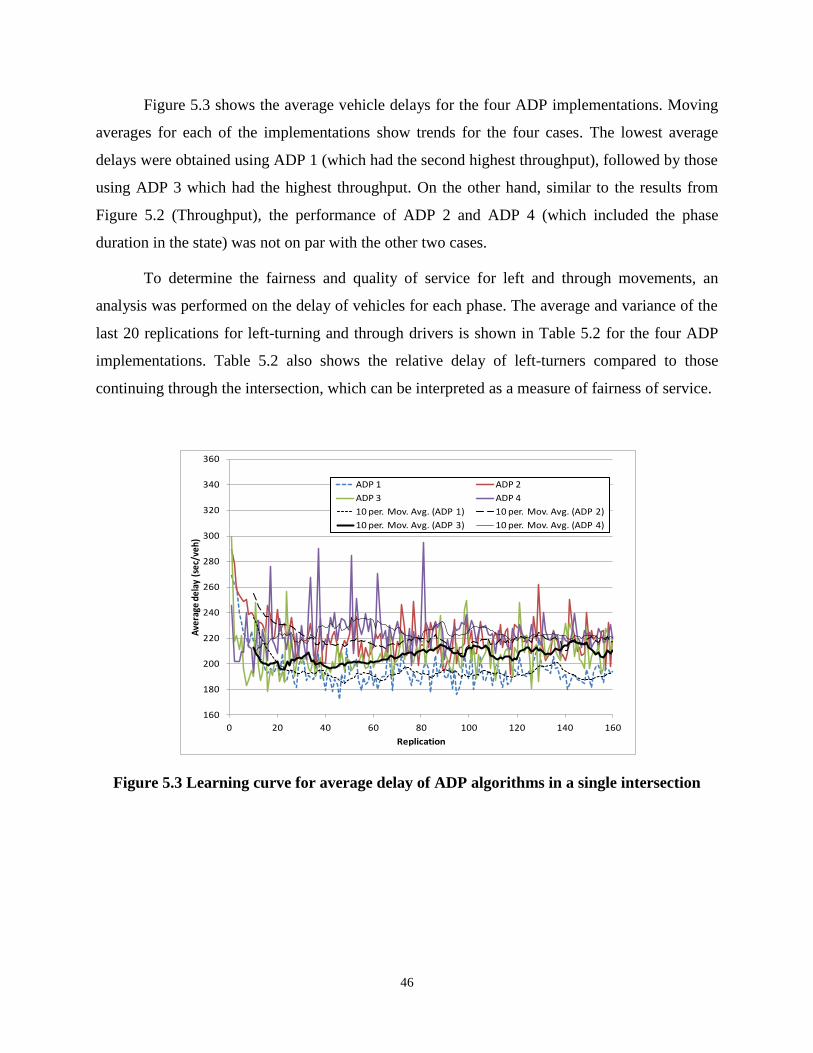
46
Figure 5.3 shows the average vehicle delays for the four ADP implementations. Moving
averages for each of the implementations show trends for the four cases. The lowest average
delays were obtained using ADP 1 (which had the second highest throughput), followed by those
using ADP 3 which had the highest throughput. On the other hand, similar to the results from
Figure 5.2 (Throughput), the performance of ADP 2 and ADP 4 (which included the phase
duration in the state) was not on par with the other two cases.
To determine the fairness and quality of service for left and through movements, an
analysis was performed on the delay of vehicles for each phase. The average and variance of the
last 20 replications for left-turning and through drivers is shown in Table 5.2 for the four ADP
implementations. Table 5.2 also shows the relative delay of left-turners compared to those
continuing through the intersection, which can be interpreted as a measure of fairness of service.
Figure 5.3 Learning curve for average delay of ADP algorithms in a single intersection
160
180
200
220
240
260
280
300
320
340
360
0 20 40 60 80 100 120 140 160
Ave
rage
del
ay (
sec/
veh)
Replication
ADP 1 ADP 2
ADP 3 ADP 4
10 per. Mov. Avg. (ADP 1) 10 per. Mov. Avg. (ADP 2)
10 per. Mov. Avg. (ADP 3) 10 per. Mov. Avg. (ADP 4)

47
Table 5.2 Delay per Phase for ADP Implementations in a Single Intersection
The lowest delay per phase was obtained with ADP 3 for the through movements, but the
most balanced service was provided using ADP 1, where the mean waiting time for both left and
through movements was practically equal. Other implementations (ADP 2 and ADP 4) were
highly unstable and provided longer delays for both left and through movements, and
significantly higher variances for the left-turn phases.
Thus, a tradeoff is found between providing more balanced service (ADP 1) and favoring
the phases with higher demands but achieving higher throughput (ADP 3). It is also noted that
even though the differences in the average signal timings between ADP 1 and ADP 3 were very
small, this resulted in significant changes in the ratio of delay between drivers in left and through
phases and the throughputs.
The average speed of all vehicles in the network is shown for the four ADP
implementations in Figure 5.4. ADP 1 had the highest average speeds, which combined with the
lowers average delays and the second highest throughput, provides a favorable performance
along with ADP 3. Similar to previous figures, Figure 5.4 shows a 10-point average speed to
highlight the learning curve as the agents gain and accumulate experience.
Mean (s) Variance (s) Mean (s) Variance (s)
ADP 1 226.3 531.6 242.5 29.6 0.93
ADP 2 251.9 17758.6 283.8 4.1 0.89
ADP 3 373.5 487.3 208.5 34.8 1.79
ADP 4 395.6 89499.7 245.1 10.8 1.61
Left-turn phases T hrough phases
Implementa tion
Ratio
Left/T hrough

48
Figure 5.4 Learning curve for average speed of ADP algorithms in a single intersection
5.1.3. Q-learning implementations
Similar to the analysis performed for ADP algorithms, a series of signal controllers were also
created for Q-learning algorithms. Four implementations using Q-learning (labeled Q1 through
Q4) follow the same state and reward definitions as explained for ADP 1 through ADP 4 in the
previous section. The analysis of the performance of these implementations is described below.
5.1.4. Performance
The first indicator to determine the performance of the algorithms was the intersection
throughput. The learning curve for the Q-learning implementations is shown in Figure 5.5, where
there was a distinctive improvement using Q1 and Q3, compared to those that had the phase
duration as part of the state representation (Q2 and Q4). This trend is similar to that observed for
the ADP implementations.
2
3
4
5
6
7
8
9
10
0 20 40 60 80 100 120 140 160
Ave
rage
Sp
ee
d (
mp
h)
Replication
ADP 1 ADP 2ADP 3 ADP 410 per. Mov. Avg. (ADP 1) 10 per. Mov. Avg. (ADP 2)10 per. Mov. Avg. (ADP 3) 10 per. Mov. Avg. (ADP 4)

49
Figure 5.5 Learning curve for throughput of Q-learning algorithms in a single intersection
A direct comparison between ADP and Q-learning is possible given that the algorithms
make use of the same information from the simulation and share the source code for data
collection and processing. In addition, the same random seeds were used for the two algorithms,
allowing for a paired comparison. Figure 5.6 shows the two most favorable implementations for
both ADP and Q-learning (implementations 1 and 3). It is observed that performance of the two
algorithms is comparable at the end of the 160 training runs, especially for Q3 and ADP 3,
reaching the highest throughput levels for the two series of implementations.
400
450
500
550
600
650
700
750
800
0 20 40 60 80 100 120 140 160
Thro
ugh
pu
t (ve
hic
les
pro
cess
ed)
Replication
C1Q C2Q
C3Q C4Q
10 per. Mov. Avg. (C1Q) 10 per. Mov. Avg. (C2Q)
10 per. Mov. Avg. (C3Q) 10 per. Mov. Avg. (C4Q)
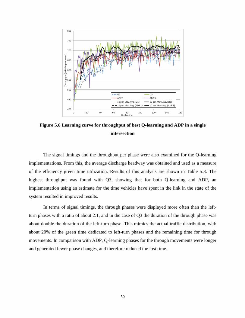
50
Figure 5.6 Learning curve for throughput of best Q-learning and ADP in a single
intersection
The signal timings and the throughput per phase were also examined for the Q-learning
implementations. From this, the average discharge headway was obtained and used as a measure
of the efficiency green time utilization. Results of this analysis are shown in Table 5.3. The
highest throughput was found with Q3, showing that for both Q-learning and ADP, an
implementation using an estimate for the time vehicles have spent in the link in the state of the
system resulted in improved results.
In terms of signal timings, the through phases were displayed more often than the left-
turn phases with a ratio of about 2:1, and in the case of Q3 the duration of the through phase was
about double the duration of the left-turn phase. This mimics the actual traffic distribution, with
about 20% of the green time dedicated to left-turn phases and the remaining time for through
movements. In comparison with ADP, Q-learning phases for the through movements were longer
and generated fewer phase changes, and therefore reduced the lost time.
400
450
500
550
600
650
700
750
800
0 20 40 60 80 100 120 140 160
Thro
ugh
pu
t (ve
hic
les
pro
cess
ed)
Replication
Q1 Q3
ADP 1 ADP 3
10 per. Mov. Avg. (Q1) 10 per. Mov. Avg. (Q3)
10 per. Mov. Avg. (ADP 1) 10 per. Mov. Avg. (ADP 3)

51
Table 5.3 Signal Timings and Average Discharge Headway for Q-learning in a Single
Intersection
The average delay for all vehicles in the system is shown in Figure 5.7 for the four Q-
learning implementations. At the end of the 160 runs the four implementations seem to converge
to the same lower delay level, with faster learning rates for the algorithms that made use of the
time vehicles have spent in the link as part of the state (Q1 and Q3).
Green EW Left Green EW Thru Green NS Left Green NS Thru Total Througput
Ave green time (s) 8 13.43 8.14 13.49
Total phase frequency 488 889 555 905
Total green time (s) 3904 11939 4518 12208
Throughput (veh) 3267 13058 3443 13430
Ave. discharge headway
(s)2.39 1.83 2.62 1.82
Ave green time (s) 8.01 10.88 8.09 10.93
Total phase frequency 505 1046 581 1026
Total green time (s) 4045 11380 4700 11214
Throughput (veh) 3075 12601 3167 12382
Ave. discharge headway
(s)2.63 1.81 2.97 1.81
Ave green time (s) 8.01 15.19 8.14 15.2
Total phase frequency 433 844 501 867
Total green time (s) 3468 12820 4078 13178
Throughput (veh) 3347 13844 3718 14245
Ave. discharge headway
(s)2.07 1.85 2.19 1.85
Ave green time (s) 8.01 10.54 8.04 10.33
Total phase frequency 535 1013 641 1058
Total green time (s) 4285 10677 5154 10929
Throughput (veh) 3229 13454 3497 13333
Ave. discharge headway
(s)2.65 1.59 2.95 1.64
Q 2 31225
Q 3 35154
Q 4 33513
Implementation IndicatorPhase
Q 1 33198

52
Figure 5.7 Learning curve for average delay of Q-learning algorithms in a single
intersection
In comparison with ADP, Figure 5.8 shows the implementations with the lowest delay for
both Q-learning and ADP, which in this case were implementations Q3 and ADP 1. The
performance of the two implementations is similar in terms of delay and this is also reflected in
their similar average discharge headway, however they yielded different throughputs (Tables 5.1
and 5.3).
160
180
200
220
240
260
280
300
320
340
360
0 20 40 60 80 100 120 140 160
Ave
rage
Del
ay (s
ec/v
eh)
Replication
Q1 Q2
Q3 Q4
10 per. Mov. Avg. (Q1) 10 per. Mov. Avg. (Q2)
10 per. Mov. Avg. (Q3) 10 per. Mov. Avg. (Q4)

53
Figure 5.8 Learning curve for average delay of best Q-learning and ADP in a single
intersection
In a more detailed examination of the delay of Q-learning, the individual phases are
observed to obtain the data shown in Table 5.4, analogous to Table 5.2 for ADP. It is observed
that the lowest overall delays were observed for left-turning drivers using Q2, but causing a
significant unbalance with delays of through vehicles. The delay of through movements was
more predictable, with variances significantly lower than those of left-turn vehicles. Better
balance of service for both directions was achieved by Q4 and Q3.
Given that the demand for through movements is 4 times greater than that of left turns, it
is not surprising that Q3 had the lowers overall delay for the whole intersection together, as seen
in Figure 5.7.
Table 5.4 Delay per Phase for Q-learning Implementations in a Single Intersection
160
180
200
220
240
260
280
300
320
340
360
0 20 40 60 80 100 120 140 160
Ave
rage
Del
ay (s
ec/v
eh)
Replication
Q3
ADP 1
10 per. Mov. Avg. (Q3)
10 per. Mov. Avg. (ADP 1)
Mean (s) Variance (s) Mean (s) Variance (s)
Q 1 179.2 248.6 256.3 76.0 0.70
Q 2 175.6 77.1 282.7 13.4 0.62
Q 3 244.5 856.2 220.3 33.8 1.11
Q 4 235.0 1443.0 239.5 4.2 0.98
Implementa tion
Left-turn phases T hrough phases Ratio
Le ft/T hrough

54
Regarding the average speed of vehicles, a summary of the performance of the four Q-
learning implementations is shown in Figure 5.9. Similar to the curve for delay, the speed of the
four cases approach a similar speed level by the time they reach the last of the 160 replications in
the learning stage.
Figure 5.9 Learning curve for average speed of Q-learning algorithms in a single
intersection
5.1.5. Summary of Findings
For a single isolated intersection, the reinforcement learning agents performed favorably by
displaying the green indication proportionally to the directional demands and each movement. Q-
learning and ADP showed similar performance and improved results as the agent accumulated
experience, indicating that a learning process was in fact taking place. Results indicate that a
measure of the occupancy or a combination of occupancy and delay for each movement was
descriptive enough for the agents to control the signal efficiently, without the need to include
2
3
4
5
6
7
8
9
10
0 20 40 60 80 100 120 140 160
Ave
rage
Sp
eed
(mp
h)
Replication
Q1 Q2
Q3 Q4
10 per. Mov. Avg. (Q1) 10 per. Mov. Avg. (Q2)
10 per. Mov. Avg. (Q3) 10 per. Mov. Avg. (Q4)

55
phase duration in the state representation. This simple case shows that a simple demand-based
only approach to control the signals could be practical for an isolated intersection.
5.2. Four-intersection Arterial, Undersaturated Conditions
The second case study to evaluate the reinforcement learning algorithms was an arterial with four
intersections. Conflicting volumes in the first two intersections create the need to continuously
change phases, and open the opportunity to observe if there is any emergent coordinated
behavior between them. The remaining two intersections did not have conflicting volumes and
the signals should learn not to provide green time to those approaches. Entry volumes on the
north and south end of the arterial are 2000 vph for the two lanes combined, and one third of the
per-lane volume was input at intersections 1 and 2, for a total of 1000 vph in the three lanes
combined. A schematic representation of the arterial is shown in Figure 5.10.
This section presents the results of multiple implementations, in a similar format to that
used for the case of a single intersection, above. The ADP implementations will be described
next, followed by Q-learning and some contrasts between the two approaches.
5.2.1. ADP Implementations
A total of four implementations were created for this scenario using ADP algorithms. The
implementation labels include the letter “a” to create a distinction between this scenario and
others.

56
Figure 5.10 Schematic representation of arterial, where “x” indicates no traffic in the
approaching links
The first two implementations (ADP1a and ADP2a) are analogous to implementations
with best performance from the previous scenario (ADP1 and ADP3). Thus, in ADP1a the state
was represented only by the number of vehicles in each link and the current phase, and in ADP2a
the state incorporates a measure of the time the vehicles have spent in the link together with the
number of vehicles. It is noted that the state space does not change from ADP1a to ADP2a, but
only the variables involved in the estimation of the current state.
The remaining two implementations (ADP3a and ADP4a) included the following
communication capabilities: 1) it was known to an agent if the receiving links of the neighboring
intersections were near capacity (implemented as a dimension in the state), and 2) the agent will
receive an incentive for providing green to incoming vehicles from adjacent intersection
1
2
3
4
1000 vph
1000 vph
2000 vph
2000 vph
375 ft
790 ft
390 ft
500 ft
500 ft
740 ft 760 ft

57
(implemented as a reduction in penalties). In addition to these capabilities, ADP4a used a
modified reward function that included potential downstream blockages, so that penalties were
created if green time was given to approaches that could result in these situations. More
specifically, penalties were gradually increased if the downstream link was occupied between 0
and 40%, between 40 and 60%, or higher than 60%, as a function of the opposing traffic.
The potential for blockage in ADP3a and ADP4a was included as an additional
dimension in the state space in the form of up to two levels of potential blockage per direction.
The additional information included in ADP4a did not affect the size of the state space, but the
calculation of the reward.
This scenario reflected undersaturated conditions, thus the total system throughput was
expected to remain similar across all implementations unless their performance is significantly
subpar compared to the others. A similar set of the indicators used in the case of a single
intersection will be also shown in this case, in combination with other indicators that are
appropriate for multiple intersections such as the total number of stops for a vehicle in the
system.
5.2.2. Performance
The analysis starts with the average delay of all vehicles in the network, as shown in Figure 5.11.
It is observed that the performance of the four implementations varied significantly, including
the last stages of the training curve. ADP3a achieved the lowest average delays and ADP1a the
highest. Recall that ADP3a included an incentive for incoming vehicles from adjacent
intersections, but so did ADP4a using a different reward function.

58
Figure 5.11 Learning curve for average delay of ADP algorithms in an arterial
Differences between the four implementations were, for the most part, the result of not
completely eliminating phase changes for the two intersections that did not have conflicting
volumes. The signals at these locations were not stable enough using ADP1a and ADP4a and the
green phase was randomly assigned to the E-W direction with some frequency. A closer view of
the signals in these two intersections showed that ADP1a provided green to the opposite
direction for about one fourth of the total green time at intersection 4 and only a negligible
portion of the green at intersection 3 (about 1% of the time). On the other hand, using ADP4a
about one sixth of the green time was allocated to the E-W direction at intersection 4, and about
5% to the E-W direction at intersection 3. The remaining two implementations did not provide
green time to approaches without demand at the end of the training process.
On the other hand, the average delay for each of the phases at the two intersections with
conflicting volumes was also inspected, as shown in Table 5.5. Overall, the average delays for
the four implementations are similar, indicating limited effects of the additional features for
ADP3a and ADP4a. This result does not come as a surprise because blockages were not expected
to be significant in undersaturated conditions.
10
15
20
25
30
35
40
45
50
55
0 10 20 30 40 50 60 70 80 90
Ave
rage
De
lay
(s/v
eh
)
Replication
ADP1a ADP2a
ADP3a ADP4a
10 per. Mov. Avg. (ADP1a) 10 per. Mov. Avg. (ADP2a)
10 per. Mov. Avg. (ADP3a) 10 per. Mov. Avg. (ADP4a)

59
Table 5.5 Delay per Phase for ADP Implementations in an Arterial
Additional information regarding the signal timings for each of the two directions of
traffic in the intersections with conflicting volumes is shown in Table 5.6. The signal timings
from ADP2a and ADP3a provided longer green times for the traffic direction along the arterial
compared to the other implementations. Likewise, the average discharge headway was slightly
longer for ADP2a and ADP3a.
In addition, the average green times for intersection 1 were longer than for intersection 2
along the arterial. This is explained by the more continuous arrival of vehicles at intersection 1
given that the demand on the northbound is reduced to about 72% of the original entry volume
due to right and left turn movements, and the demand southbound to about 95%. This is also an
indication that, given the greater demand southbound, coordination should be provided in this
direction. The offsets between the beginning of green time at intersections 1 and 2 on the
southbound and on the northbound were explored to determine if the coordination occurred as
expected.
For the southbound, the offsets of the last 20 replications (at the end of the training
period) were found to be shorter than those for northbound and closer to an ideal offset given the
distance between intersections. The ideal offset assuming no initial queue was around 10 seconds
in free-flow speed, but closer to 15 seconds with the assigned demands. A plot of the cumulative
distribution of the offsets using ADP3a showed that 70% of the offsets in the southbound
direction were lower than 22 seconds, whereas in the southbound the 70% of the cumulative
distribution was located at 34 seconds. This is a clear indication of better coordination in the
southbound, as expected. In contrast, an implementation without the coordination features (using
Mean (s) Variance (s) Mean (s) Variance (s)
ADP1a 15.4 269.6 25.0 2.1
ADP2a 18.8 225.8 17.3 0.8
ADP3a 16.3 280.3 23.3 2.4
ADP4a 16.0 284.7 23.1 2.3
ADP1a 10.3 81.5 20.7 1.4
ADP2a 11.7 117.8 18.0 0.6
ADP3a 11.5 125.6 20.8 2.4
ADP4a 11.1 116.9 21.5 2.4
Intersection 1
Intersection 2
Inte rsection Implementa tionN-S phase E-W phase

60
ADP2a) showed that 70% of the offsets were slightly longer in both directions, with the
southbound direction at 24 seconds and for the northbound at 38 seconds.
Table 5.6 Signal Timings and Average Discharge Headway for ADP in Arterial
Another measure of the coordination of traffic along the arterial is the average number of
stops per vehicles. Even though this indicator does not account for vehicles slowing down, it
may show when coordination was significantly different between the implementations. This is
shown in Figure 5.12, where ADP2a and ADP3a, following the same trend observed for the
delay, and closely linked to the signal operation in intersections 3 and 4.
E-W N-S Total Througput E-W N-S Total Througput
Ave green
time (s)8.07 24.89 8.3 20.77
Total phase
frequency877 876 974 977
Total green
time (s)7082 21810 8092 20294
Throughput
(veh)9912 34402 9994 33964
Ave.
discharge
headway (s)
2.14 2.54 2.43 2.39
Ave green
time (s)8.01 30.42 8.04 21.67
Total phase
frequency769 777 952 956
Total green
time (s)6164 23640 7654 20716
Throughput
(veh)9919 34375 9939 34010
Ave.
discharge
headway (s)
1.86 2.75 2.31 2.44
Ave green
time (s)8.07 26.57 8.06 22.71
Total phase
frequency850 849 930 931
Total green
time (s)6860 22558 7496 21143
Throughput
(veh)10008 34315 9999 33948
Ave.
discharge
headway (s)
2.06 2.63 2.25 2.49
Ave green
time (s)8.11 23.42 8.15 21.52
Total phase
frequency907 908 953 953
Total green
time (s)7360 21270 7766 20508
Throughput
(veh)9907 34392 9956 34033
Ave.
discharge
headway (s)
2.23 2.47 2.34 2.41
ADP 2a 44294 43949
ADP 3a 44323 43947
Implementation Indicator
ADP 1a 43958
Intersection 1 Intersection 2
44314
ADP 4a 44299 43989

61
Figure 5.12 Learning curve for average number of stops of ADP algorithms in an arterial
Agent policies along the arterial were analyzed to determine if the results at the
individual intersection level followed expected behavior. Two intersections were analyzed under
specific states to observe the value of being at a given state using ADP3a: intersections 1 and 4
from Figure 5.10.
The most straight forward analysis would be at intersection 4, where there were no
conflicting volumes in the E-W direction for the N-S arterial. The values of the states along the
arterial at intersection 4 were obtained in cases without blockages when the N-S state varied
from 0 to 14. Each of these states was visited more than 20 times, thus their values had been
updated repeatedly for the analysis. Notice that the E-W state was always zero, and therefore
their values were never updated from the initial zero value.
Figure 5.13 shows the increase in the value function as the state increases. Since all
values in Figure 5.13 are greater than zero, and increasing with the state, there is more pressure
to continue the green phase on the arterial with more vehicles in the link. On the other hand,
there is no pressure to change the phase to the minor street since the values of those states
remained zero. This policy resulted in the green indication given to the arterial at all times.
0.4
0.6
0.8
1
1.2
1.4
1.6
1.8
2
0 10 20 30 40 50 60 70 80
Ave
rage
sto
ps
pe
r ve
hic
le
Replication
ADP1a ADP2aADP3a ADP4a10 per. Mov. Avg. (ADP1a) 10 per. Mov. Avg. (ADP2a)10 per. Mov. Avg. (ADP3a) 10 per. Mov. Avg. (ADP4a)

62
Figure 5.13 State values for intersection 4 (N-S direction) along arterial
A more interesting comparison of the policies can be observed at intersection 1, where
conflicting volumes were present. Policies can be observed as the number of vehicles in the
arterial changes. Figure 5.14 shows that if the value of the state increases, the pressure to keep
providing green time to this direction increases at an almost linear rate. This applies for the
whole range of the volumes in the crossing street, but it is more pronounced if the crossing
volume is lower. This is expected, since the lower the pressure to change the green indication to
the side street, the greater the unit change in the state value with a unit increase in the arterial
state.
0
5
10
15
20
25
30
0 2 4 6 8 10
Val
ue
of
the
sta
te
N-S State (E-W State=0)

63
Figure 5.14 State values for intersection 1 – conflicting volumes in E-W and N-S
The exploration of the policies along the arterial helps validating the convergence of the
state values after the agents were trained. Recall that Figures 5.13 and 5.14 are based on values
of states that have been visited more than 5 times and up to more than 1000 times, thus they have
been updated multiple times to help approximating the converged state values.
5.2.3. Q-learning Implementations
Four implementations similar to those explained above for ADP where used to test the
performance of Q-learning in the arterial scenario, labeled Q1a through Q4a. There is
correspondence between the labeling used in this subsection and the characteristics of the
implementations for ADP, thus for example the implementation for Q1a had the same state and
reward definitions of ADP1a.
Unlike the results for ADP all four cases using Q-learning had similar performance at the
end of the 80 training runs and reached the same levels of the best ADP cases.

64
5.2.4. Performance
The first indicator used in this analysis was the average delay per vehicle in the system, as shown
in Figure 5.15. The four Q-learning implementations converged to a similar delay value and
produced similar variations on the replications. An examination of the delays per intersection
showed that in one of the implementations (Q1a) the signals provided momentarily the right of
way to the approaches with no demand, delaying vehicles unnecessarily. In Q1a the signals
provided on average about 5% of the total green time to the approaches with no demand, which
accounts for some of the increased total delay of Q1a compared to the other algorithms in Figure
5.15. Additional reinforcement from adding an estimate of delay in the state, as well as incentive
from adjacent intersections had a better effect in preventing switching phases to approaches with
no demand in the Q-learning implementations compared to ADP.
Figure 5.15 Learning curve for average delay of Q-learning algorithms in an arterial
Delay values for the two intersections with opposing demands are shown in Table 5.7.
Delays for the N-S direction were in general lower than for the E-W direction, which may be at
first counterintuitive given the greater demand on the N-S direction, but it can be mainly
10
15
20
25
30
35
40
45
50
55
0 10 20 30 40 50 60 70 80
Ave
rage
De
lay
(s/v
eh
)
Replication
Q1a Q2a
Q3a Q4a
10 per. Mov. Avg. (Q1a) 10 per. Mov. Avg. (Q2a)
10 per. Mov. Avg. (Q3a) 10 per. Mov. Avg. (Q4a)

65
explained by the greater number of vehicles that could be processed without stopping due to
increased pressure to hold the green light. The larger variance of the delay for the N-S direction
also explains this situation, where some vehicles may have been processed by the intersection
without stopping but some others had to wait at least the minimum green time and yellow-red
transition of the E-W direction. On the other hand, vehicles in the E-W direction were likely to
wait for the duration of the N-S direction (a great portion of a typical cycle) to be processed in
the next green light, having a more constant delay. Lastly, a slight decrease in the delay of the
intersections on the N-S direction (along the arterial) can be observed when using Q4a (which
accounted for incentive upon arrival of platoons) but at the expense of greater delay for the E-W
direction.
Similar comments to those mentioned for the ADP implementations apply to these cases
with Q-learning in relation to the magnitude of the mean and variance of the delay.
Table 5.7 Delay per Phase for Q-learning Implementations in an Arterial
The characteristics of the signal timings and the average discharge headway for the four
implementations are shown in Table 5.8. As expected, given the undersaturated conditions, all
four algorithms processed a very similar number of vehicles. Slightly different discharge
headways were observed using Q3a and Q4a compared to Q1a and Q2a, favoring the N-S
direction (larger headways) and also signal progression.
Different from ADP, the average phase duration for both N-S and E-W directions are
more similar between intersections 1 and 2, creating a better probability of coordination in both
directions due to common cycle length. If this is true, the offsets in both directions should be
Mean (s) Variance (s) Mean (s) Variance (s)
Q1a 17.1 267.4 21.4 1.2
Q2a 17.1 208.1 17.6 1.0
Q3a 17.5 284.6 19.6 1.7
Q4a 16.0 284.7 23.1 2.3
Q1a 13.3 156.4 15.5 0.4
Q2a 13.4 150.5 15.2 0.7
Q3a 12.3 136.3 18.1 1.1
Q4a 11.1 116.9 21.5 2.4
Intersection 1
Intersection 2
Inte rsection Implementa tionN-S phase E-W phase
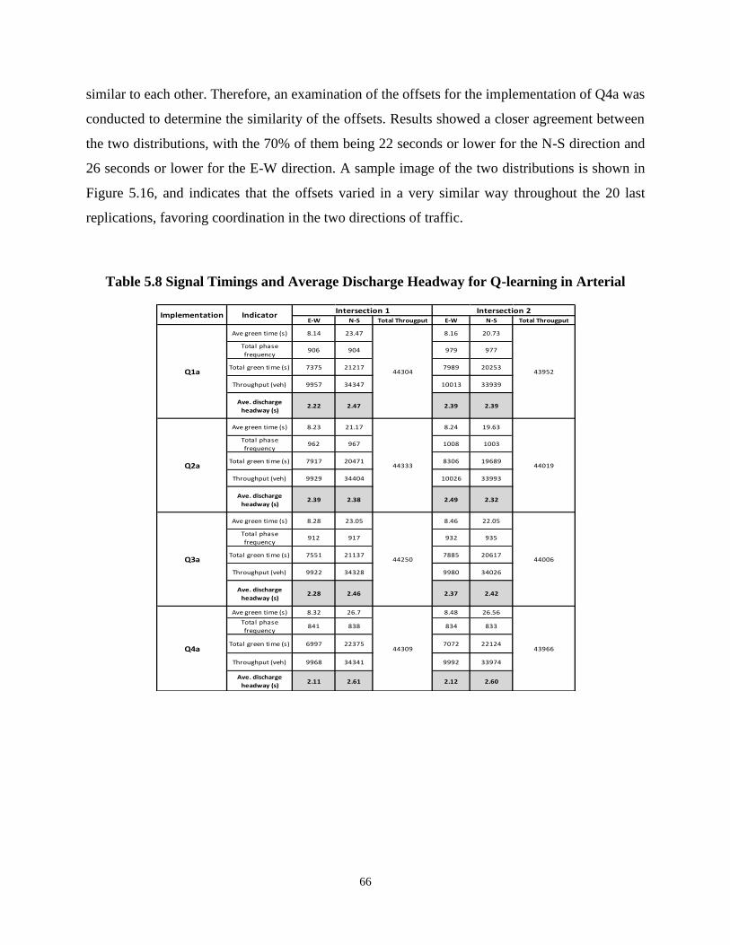
66
similar to each other. Therefore, an examination of the offsets for the implementation of Q4a was
conducted to determine the similarity of the offsets. Results showed a closer agreement between
the two distributions, with the 70% of them being 22 seconds or lower for the N-S direction and
26 seconds or lower for the E-W direction. A sample image of the two distributions is shown in
Figure 5.16, and indicates that the offsets varied in a very similar way throughout the 20 last
replications, favoring coordination in the two directions of traffic.
Table 5.8 Signal Timings and Average Discharge Headway for Q-learning in Arterial
E-W N-S Total Througput E-W N-S Total Througput
Ave green time (s) 8.14 23.47 8.16 20.73
Total phase
frequency906 904 979 977
Total green time (s) 7375 21217 7989 20253
Throughput (veh) 9957 34347 10013 33939
Ave. discharge
headway (s)2.22 2.47 2.39 2.39
Ave green time (s) 8.23 21.17 8.24 19.63
Total phase
frequency962 967 1008 1003
Total green time (s) 7917 20471 8306 19689
Throughput (veh) 9929 34404 10026 33993
Ave. discharge
headway (s)2.39 2.38 2.49 2.32
Ave green time (s) 8.28 23.05 8.46 22.05
Total phase
frequency912 917 932 935
Total green time (s) 7551 21137 7885 20617
Throughput (veh) 9922 34328 9980 34026
Ave. discharge
headway (s)2.28 2.46 2.37 2.42
Ave green time (s) 8.32 26.7 8.48 26.56
Total phase
frequency841 838 834 833
Total green time (s) 6997 22375 7072 22124
Throughput (veh) 9968 34341 9992 33974
Ave. discharge
headway (s)2.11 2.61 2.12 2.60
Q3a 44250 44006
Q4a 44309 43966
Intersection 1 Intersection 2
Q1a 44304 43952
Q2a 44333 44019
Implementation Indicator

67
Figure 5.16 Distribution of Offsets for NB and SB in intersections 1 and 2 using Q4a
The total number of stops per vehicle was also monitored for the whole system, and it is
shown in Figure 5.17. The four implementations converged to a value of about 0.7 stops per
vehicle, with an edge for the Q4a implementation. This was also expected given the longer
average green time for the N-S direction in Q4a compared to the other implementations and the
similar timings for the two intersections with conflicting movements, as shown above.
Figure 5.17 Learning curve for average number of stops of Q-learning algorithms in
arterial
0.4
0.6
0.8
1
1.2
1.4
1.6
1.8
2
0 10 20 30 40 50 60 70 80
Ave
rage
sto
ps
pe
r ve
hic
le
Replication
Q1a Q2a
Q3a Q4a
10 per. Mov. Avg. (Q1a) 10 per. Mov. Avg. (Q2a)
10 per. Mov. Avg. (Q3a) 10 per. Mov. Avg. (Q4a)
Offset (s)
Cumulative
Probability

68
In comparison with the best ADP, the learning curve of the Q-learning implementation
was very similar, with slight benefits in terms of the number of stops for Q-learning. This can be
observed in Figure 5.18, showing ADP3s and Q4a.
Figure 5.18 Comparison of learning curves for average number of stops of Q4a and ADP3a
The performance of the best ADP and Q-learning algorithms was also compared to the
results of the traffic signal optimization performed by the commercial software package
TRANSYT7F, which uses a search in the solution space through a genetic algorithm. The traffic
environment for TRANSYT7F was provided by CORSIM, a well known microscopic simulator.
The arterial was coded in CORSIM with the exact same characteristics as in VISSIM. In
addition, calibration had to be performed to ensure that the vehicle characteristics, the discharge
headways and speeds were the same in the two simulation environments. The following variables
were modified in VISSIM to attain the desired calibration: desired speed, vehicle types were
limited to two, with the same dimensions and similar operational characteristics, the additive part
of the desired safety distance in the car-following model (to obtain similar discharge headways),
and the standstill distance of vehicles (to match the number of vehicles that a link could store). It
is noted that the decision to perform this comparison was made before obtaining VISSIM results
presented above, therefore all data was obtained after the calibration was performed.
0.4
0.6
0.8
1
1.2
1.4
1.6
1.8
2
0 10 20 30 40 50 60 70 80
Ave
rage
sto
ps
pe
r ve
hic
le
Replication
Q4a
ADP3a
10 per. Mov. Avg. (Q4a)
10 per. Mov. Avg. (ADP3a)
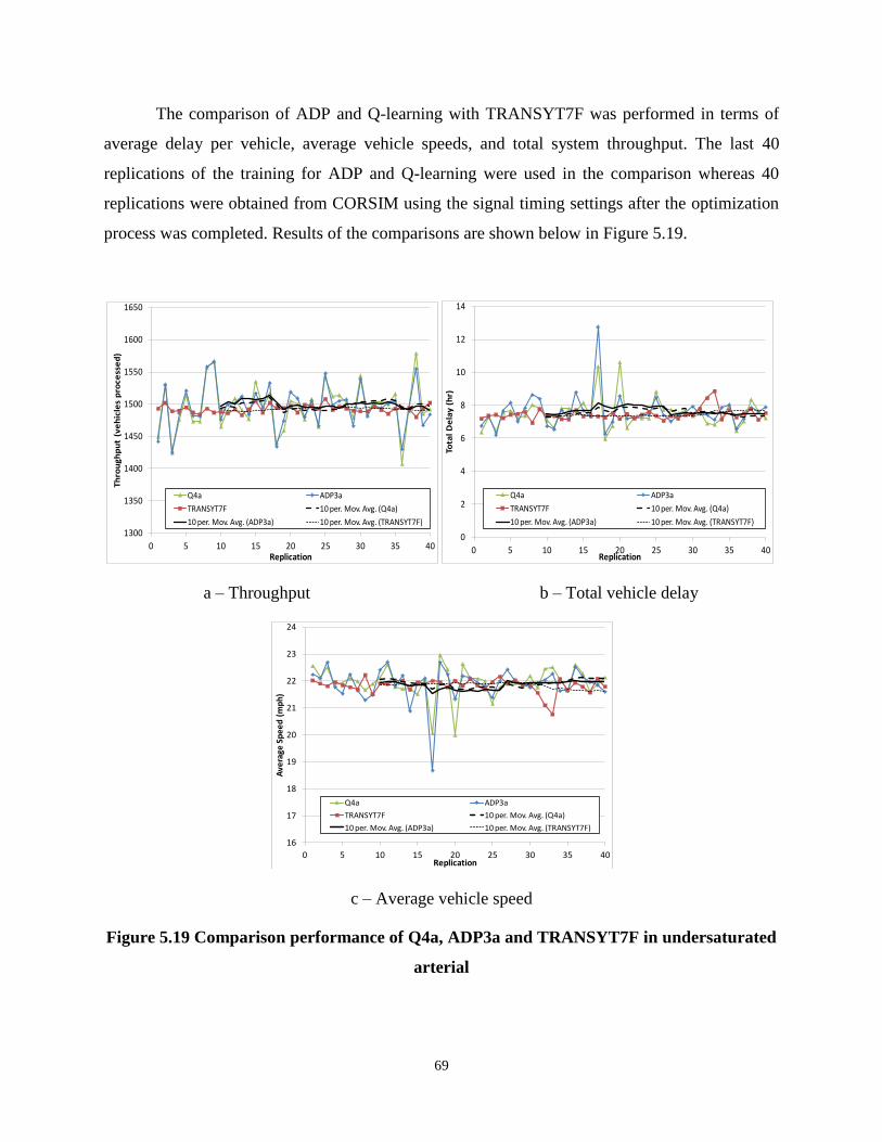
69
The comparison of ADP and Q-learning with TRANSYT7F was performed in terms of
average delay per vehicle, average vehicle speeds, and total system throughput. The last 40
replications of the training for ADP and Q-learning were used in the comparison whereas 40
replications were obtained from CORSIM using the signal timing settings after the optimization
process was completed. Results of the comparisons are shown below in Figure 5.19.
a – Throughput b – Total vehicle delay
c – Average vehicle speed
Figure 5.19 Comparison performance of Q4a, ADP3a and TRANSYT7F in undersaturated
arterial
1300
1350
1400
1450
1500
1550
1600
1650
0 5 10 15 20 25 30 35 40
Th
rou
gh
pu
t (v
eh
icle
s p
roce
sse
d)
Replication
Q4a ADP3a
TRANSYT7F 10 per. Mov. Avg. (Q4a)
10 per. Mov. Avg. (ADP3a) 10 per. Mov. Avg. (TRANSYT7F)
0
2
4
6
8
10
12
14
0 5 10 15 20 25 30 35 40
Tota
l D
ela
y (
hr)
Replication
Q4a ADP3a
TRANSYT7F 10 per. Mov. Avg. (Q4a)
10 per. Mov. Avg. (ADP3a) 10 per. Mov. Avg. (TRANSYT7F)
16
17
18
19
20
21
22
23
24
0 5 10 15 20 25 30 35 40
Ave
rage
Sp
ee
d (
mp
h)
Replication
Q4a ADP3a
TRANSYT7F 10 per. Mov. Avg. (Q4a)
10 per. Mov. Avg. (ADP3a) 10 per. Mov. Avg. (TRANSYT7F)

70
Figure 5.19 shows similar average values for all three methods for the three indicators.
However, higher variation between different replications was obtained in VISSIM compared to
CORSIM. It is important to observed that while the same random seeds where used for ADP and
Q-learning, this was not possible with CORSIM, as the simulation packages had a different car
following model, and therefore different use of random numbers. This variation can be better
observed in 19a, where the vehicle throughput is shown for the different replications.
5.2.5. Summary of Findings
Similar to the results for an isolated intersection, Q-learning and ADP agents efficiently
controlled the traffic signals along an arterial. The features included in the state and reward
functions had significant impact on the performance of the signals. Incentives for arriving
upstream platoon of vehicles and penalties to prevent blockages improved the coordination
between intersections by reducing the average number of stops through more adequate offsets.
These features also added stability on the cases where no conflicting volumes were present. Q-
learning seems to have an edge in terms of signal control for the cases without conflicting, as
expected given the direct association between states and actions.
Results also indicate that the ADP and Q-learning implementations were as effective as
current commercial solutions to find optimal signal timings along an arterial in undersaturated
conditions. These findings are also used as building blocks for more complex scenarios described
in the following sections.
5.3. Five-intersection Arterial – Q-learning, Variable Demands
In this scenario, three different sets of time-varying demands were tested along a five-
intersection arterial to determine how well the agents adjusted to changing conditions. The
reactions of agents to variable demands help providing answers to the problem of non-stationary
conditions for the traffic control domain. Agents were provided with communication capabilities
in order to share limited information regarding their current state, and therefore improve
coordination.

71
A sample image of the arterial and the intersecting streets is given in Figure 5.20, where
the vehicle entry points are marked by arrows. No turning movements were allowed, and all of
the approaching links had two lanes and were equipped with loop detectors at their entry and exit
points.
Figure 5.20 Schematic representation of the arterial and minor streets, and example of
detector location for intersection No. 2.
5.3.1. Implementation
A Q-learning implementation to similar those described above in the previous two scenarios was
used for this case. The state representation included the following components: The number of
vehicles and the time they have spent in the link (one component for E-W and one for N-S
directions), two components describing the occupancy of the links in upstream intersections (one
per direction), two components to avoid intersection blockages due to oversaturated conditions
(one per direction), the current state of the signal, and the number of time periods since the last
phase change as an indication of phase duration.
The reward structure followed the general definition provided in the description of
MASTraf from the previous Chapter, thus including the following components: a) the number of
vehicles in approaches receiving green (xg), b) the number of vehicles in approaches given red
(xr), c) a penalty for the delay incurred during the yellow-red transition when a phase is
terminated (pt), d) a penalty for giving green to approaches with congested receiving
Arterial St.
EB
Minor St. 1 Minor St. 2 Minor St. 3
WB
Minor St. 4 Minor St. 5

72
(downstream) links (pd), and e) an incentive to give green to approaches expected to receive
several vehicles from upstream links (iu). Each of these factors had a weight in the final reward
(R) in the general form of the reward equation shown below, where βi is a factor weight.
R = β1xg + β2xr + β3pt + β4pd + β5iu (5.1)
Based on the objectives of the signal control problem, the weights for the number of
vehicles in approaches with the green light (β1) and for coordinating the signals along the main
arterial (β5) were positive. On the other hand, the weights for other factors that may contribute to
delay and the number of stops (β2, β3, β4) were negative. Specifically, the weights used for the
βi factors were:
β1 = 1.5, β2 = −1, β3 = −1, β4 = 0, β5 = 1.5 (5.2)
Note that the factor including the penalty for downstream blockage due to congested
receiving links (β4) was zero. This was the case, since it was observed that the incentive for
coordination (β5) generated a “domino” effect that discharged links getting close to the
saturation points, preventing downstream blockages without having to define an explicit penalty
for them.
The reward structure in its basic form will generate a behavior that represents basic
principles of best effort policies at a given intersection. Thus, longer queues (or higher state) will
tend to receive the green indication. The immediate reward should indicate the value of a state
given the current conditions on the competing links, in addition to considerations of lost time,
downstream congestion, etc. An example of the policy based on immediate rewards at states
without blockages, at the shortest possible phase duration and considering lost time, is shown in
Figure 5.21 for illustration purposes. Figure 5.21 shows the variation of the immediate reward
for an intersection that is currently giving the green indication to the E-W approaches.

73
Figure 5.21 Immediate rewards for intersection without blockages, short phase duration,
and currently displaying green on the EW direction
Scenarios with variable traffic along the arterial were created to test the agents. The five
agents (one per intersection) were structured in an identical way, but with separate Q matrices.
Particular interest was centered on scenarios with high volume along the arterial, since
coordination can potentially pay off in greater proportion in presence of big platoons of vehicles.
Three scenarios with high traffic conditions were designed to determine the capabilities
of the agents (see Table 5.9). While all three scenarios show high total volumes, Scenario 1
presents a situation with high volume along the arterial compared to the volume in the minor
streets, Scenario 2 presents more balanced volumes, with similar traffic for the arterial and minor
streets, and Scenario 3 presents the highest conflicting volumes, close to roadway capacity.
The agents were trained prior to the actual evaluation of their performance in a
continuous fashion, not following an episodic training as in the cases from previous sections. The
training lasted for 20000 simulation seconds under each of the expected traffic volumes. The
simulation software could run at a speed about 30 times faster than real time using a PC with two
processors (2.4GHz each) and 4 GB of memory, thus the training was completed in reasonable
time.
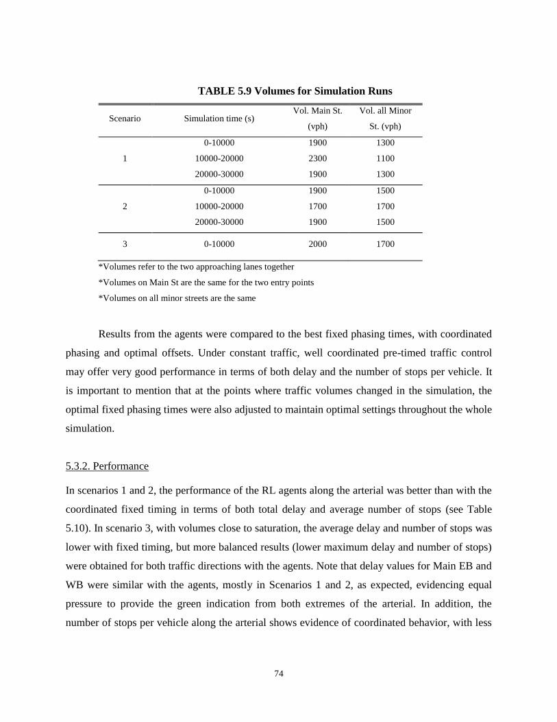
74
TABLE 5.9 Volumes for Simulation Runs
Scenario Simulation time (s) Vol. Main St.
(vph)
Vol. all Minor
St. (vph)
1
0-10000 1900 1300
10000-20000 2300 1100
20000-30000 1900 1300
2
0-10000 1900 1500
10000-20000 1700 1700
20000-30000 1900 1500
3 0-10000 2000 1700
*Volumes refer to the two approaching lanes together
*Volumes on Main St are the same for the two entry points
*Volumes on all minor streets are the same
Results from the agents were compared to the best fixed phasing times, with coordinated
phasing and optimal offsets. Under constant traffic, well coordinated pre-timed traffic control
may offer very good performance in terms of both delay and the number of stops per vehicle. It
is important to mention that at the points where traffic volumes changed in the simulation, the
optimal fixed phasing times were also adjusted to maintain optimal settings throughout the whole
simulation.
5.3.2. Performance
In scenarios 1 and 2, the performance of the RL agents along the arterial was better than with the
coordinated fixed timing in terms of both total delay and average number of stops (see Table
5.10). In scenario 3, with volumes close to saturation, the average delay and number of stops was
lower with fixed timing, but more balanced results (lower maximum delay and number of stops)
were obtained for both traffic directions with the agents. Note that delay values for Main EB and
WB were similar with the agents, mostly in Scenarios 1 and 2, as expected, evidencing equal
pressure to provide the green indication from both extremes of the arterial. In addition, the
number of stops per vehicle along the arterial shows evidence of coordinated behavior, with less

75
than 1.5 stops to traverse the 5 intersections. Even in Scenario 3, the number of stops was on
average less than 2.5 for both directions.
Regarding the minor streets (see Tables 5.11 and 5.12), for scenarios 1 and 2 the delays
and number of stops with the RL agents were also lower than with the fixed timing. It is noted
that with the RL agents, the intersection located half way in the arterial (Intersection 3) had the
highest delays and number of stops. This is a clear indication of more variability in the arrival of
traffic on the arterial since it depended on the green indications of both Minor 1 and 2 for the EB
traffic, and on both Minor 4 and 5 for the WB traffic.
TABLE 5.10 Performance of Pretimed and RL Agents for the Arterial
Scenario Strategy Delay (s) Stops per
Vehicle
Main
EB
Main
WB
Main
EB
Main
WB
1 Pretimed 22.5 103.6 0.67 4.00
Agents 37.6 35.1 1.50 1.53
2 Pretimed 22.5 73.9 0.71 3.34
Agents 34.1 32.7 1.44 1.25
3 Pretimed 21.7 90.3 0.71 3.66
Agents 59.2 49.1 2.49 2.13
TABLE 5.11 Delay - Pretimed and RL Agents for Minor Streets
Scenario Strategy Delay(s)
Minor
1
Minor
2
Minor
3
Minor
4
Minor
5
1 Pretimed 18.8 20.9 22.4 33.5 21.3
Agents 17.3 15.7 37.6 17.4 16.3
2 Pretimed 19.7 45.1 21.7 24.7 22.6
Agents 17.3 17.4 34 21.1 19.8
3 Pretimed 37.9 45.6 21.8 34.1 37.3
Agents 40.6 38.2 59.4 33.2 37.6

76
TABLE 5.12 Stops per Vehicle - Pretimed and RL Agents for Minor Streets
Scenario Strategy Stops per Vehicle
Minor
1
Minor
2
Minor
3
Minor
4
Minor
5
1 Pretimed 0.75 0.82 0.67 1.20 0.83
Agents 0.83 0.78 1.55 0.82 0.78
2 Pretimed 0.77 1.55 0.67 0.91 0.85
Agents 1.25 1.26 1.40 1.19 1.25
3 Pretimed 1.34 1.55 0.72 1.23 1.32
Agents 2.27 2.13 2.54 1.78 2.09
In terms of the signal timings, there was also evidence of signal coordination in the
duration of the green times obtained with the RL agents. An example of this situation is shown in
Figure 5.22, where the distribution of green times on the arterial road is shown for the five
intersections with two different traffic volumes. It is observed that even though the agents are not
constrained to any limitation on the green time (except a minimum green of 14 seconds), the
distribution of green times are very alike for all 5 intersections in the same time periods.
Figure 5.22 Green times for the arterial road. Left: first third of simulation in Scenario 2;
Right: second third of simulation in Scenario 2
5.3.3. Summary of Findings
In summary, results show that the agents adequately distributed the average vehicle delay and the
number of stops per vehicle for the traffic along the arterial. In addition, there was clear evidence
of traffic progression given that the average number of vehicle stops to traverse the 5
0
20
40
60
80
100
120
140
160
180
200
10 20 30 40 50
Freq
uenc
y
Duration of Green (s)
Intersection 1
Intersection 2
Intersection 3
Intersection 4
Intersection 5
0
10
20
30
40
50
60
70
80
10 20 30 40 50 60
Freq
uen
cy
Duration of Green (s)
Intersection 1Intersection 2
Intersection 3
Intersection 4
Intersection 5

77
intersections along the arterial was in the order of 1.5 stops or lower, and also by the similar
distribution of green times for all intersections during the same time periods. Even though the
performance of the RL agents was superior to the best coordinated fixed timing for high
volumes, the agents did not achieve similar results under close-to-saturation conditions. Since a
balance between the arterial and the minor streets was pursued by the agents, this created shorter
phases and increased the lost time due to yellow-red transitions.
5.4. 3x2 and 3x3 Networks – Q-learning
In these scenarios, testing was conducted for a Q-learning implementation based on the same
state and reward structure, as well as the same update rule and action selection policy as in the
previous example (along an arterial). The two scenarios included: a) a network of size 2x3; and
b) a network of size 3x3. All approaches had two lanes and no turning movements were allowed.
The main roadways had two-way traffic and the minor streets had only one-way traffic. A
schematic representation of the 2x3 network is shown in Figure 5.23 for illustration purposes.
Figure 5.23 Schematic representation of 2x3 network
The two scenarios were tested under two different volume conditions: a) high volume,
undersaturated conditions, and b) high volume, close-to-saturation conditions. For the
Minor St. 1 Minor St. 2 Minor St. 3
Corridor 1
Corridor 2

78
undersaturated conditions, 1700 vph were input at each of the entry points. For the close-to-
saturated conditions, 300 vph were added to the arterials in each direction, so that the total
volume to be processed at a given intersection was the sum of 1700 vph from the minor road,
2000 vph in the EB and 2000 vph in the WB of the arterial.
5.4.1. Implementation
The RL agents were trained during 60000 simulation seconds for the 2x3 and 3x3 networks.
Results were compared to the best pre-timed signal timing settings under the specified volumes.
The values provided here are based on the last 2 hours of simulation time from a run where the
agents used the policies created in the training period. A value was obtained from VISSIM every
5 minutes of simulation time, thus a total of 24 values were obtained from the last 2 hours of
simulation.
Given that traffic volumes per hour did not change in the simulation, pre-timed signal
operation was expected to provide adequate results. In addition, the pre-timed signals were set
such that one direction of traffic was coordinated along the two-way arterials, and also along the
one-way roadways (minor streets).
Results from the pre-timed and the reinforcement learning agents were compared in terms
of delay. A group of data collection points were defined in the networks to obtain the measures
of performance. These points covered roadway sections starting at about 200 ft upstream from
the initial signal, and ending about 200 ft after the last signal. For example, in the 2x3 network,
the delay along one of the arterials started upstream from the first traffic signal and ended
downstream of the third (and last) traffic signal.
5.4.2. Performance
The first scenario (2x3 intersections) is analyzed next. The results in terms of delays are shown
in Tables 5.13 and 5.14 for undersaturated and close-to-saturation conditions, respectively. The
average, maximum, and minimum delays per vehicle for each of the links in the networks are
included. In the pre-timed case, it is obvious that the coordinated traffic in the main corridor was
the eastbound (EB) direction.
From Table 5.13, the first observation is that lower average delay was obtained with RL
compared to the pre-timed signals. Second, there is more balance between the delays in the EB

79
and the WB direction when using the agents than in the pre-timed case. This is expected since
one direction is typically coordinated with pre-timed signals, increasing the expected delays for
the traffic in the other direction. Third, the maximum and minimum delays experienced by a
vehicle were lower using the agents compared to the pre-timed signals. Overall, it could be said
that for this specific condition, the reinforcement learning agents showed better performance that
the pre-timed signals.
Table 5.13 Delay for the 2x3 Network with High Volume and Undersaturated Conditions
Regarding Table 5.14, the operation of the RL agents in the close-to-saturation condition
was, in general, superior to pre-timed settings. This is similar to the case described above
(undersaturated condition). On average, delays on the two corridors were lower with the agents,
with a tendency to prioritize the WB direction, generating higher delays for the EB traffic.
Results from the second scenario (3x3 intersections) are shown in Tables 5.15 and 5.16.
The performance of the agents in these two cases was better than the pre-timed signal timings.
For the undersaturated conditions, average delays were lower and more balanced with the agents,
which also resulted in lower maximum and minimum values.
For the case close to saturation, also lower average, maximum, and minimum values were
obtained (see Table 5.16). Similar to the results in the 2x3 network, the agents learned policies
that generated improved and more balanced results. In particular, note that the ratio of delay
from the EB and the WB for corridor #3 is close to 1 using the agents, but more than 3 for the
pre-timed signals. Particular importance is given to corridor #3 because greater coordination
effects are expected to be seen as the traffic progresses along the minor streets in the network,
from corridor #1 through #3. Note how in Table 5.16 there is a decreasing trend in the delays
from corridor #1 to #3.
Average Max Min Average Max Min
EB 3216 21.7 36.6 16.7 3349 30.0 50.0 16.9
WB 3329 69.3 85.2 57.4 3356 23.1 37.0 15.2
EB 3269 20.1 26.2 15.0 3370 28.3 43.2 18.7
WB 3392 70.0 84.5 56.8 3370 20.1 34.2 10.0
3188 41.2 54.0 35.6 3289 45.7 67.3 28.3
3328 44.2 53.6 38.7 3318 54.7 70.3 36.0
19722 44.7 20052 33.6
Minor St. 1
Minor St. 2
Totals
Delay (veh/s) Delay (veh/s)# of
vehicles
Corridor 2
Pretimed# of
vehicles
Reinforcement Learning
Corridor 1
LinkDirection
of Traffic

80
Table 5.14 Delay for the 2x3 Network with High Volume and Close-to-saturated Conditions
Table 5.15 Delay for the 3x3 Network with High Volume and Undersaturated Conditions
Table 5.16 Delay for the 3x3 Network with High Volume and Close-to-saturated Conditions
This trend is more clearly described in Figure 5.24, where the average numbers of stops
per vehicle for each link in the 3x3 network are shown. The effect of using information from
neighboring intersections works in two ways: 1) as vehicles move toward the center of the
Average Max Min Average Max Min
EB 3526 93.4 152.1 61.7 3856 91.0 114.6 76.3
WB 3971 65.8 89.0 53.5 3910 43.8 74.3 21.0
EB 3938 22.8 35.9 14.4 4051 57.7 100.9 25.2
WB 3916 58.1 75.8 46.5 4091 40.2 64.9 22.7
2376 102.7 155.2 71.3 3703 97.6 143.4 75.1
3305 54.7 74.8 41.3 3962 45.3 113.7 29.0
4093 25.4 39.7 14.7 3983 58.1 101.2 22.6
21032 68.3 27556 61.4Totals
Corridor 1
Corridor 2
Minor St. 1
Minor St. 2
Minor St. 3
LinkDirection
of Traffic
Pretimed Reinforcement Learning# of
vehicles
Delay (veh/s) # of
vehicles
Delay (veh/s)
Average Max Min Average Max Min
EB 3350 55.8 159.7 15.4 3439 57.2 132.5 18.1
WB 3456 71.7 82.5 62.5 3420 32.9 100.2 13.7
EB 3495 24.9 43.6 16.7 3495 44.7 75.8 23.2
WB 3564 73.1 90.6 56.5 3564 24.5 40.7 13.0
EB 3403 18.4 31.4 13.2 3385 22.6 36.6 12.7
WB 3507 72.1 83.1 65.2 3486 23.9 36.9 14.1
3463 56.8 135.0 18.4 3333 52.5 86.4 20.1
3371 71.4 110.1 61.0 3438 30.0 61.9 16.5
3462 24.1 48.0 15.0 3411 42.9 85.5 17.5
27609 44.2 27560 30.1
Minor St. 1
Minor St. 2
Totals
Delay (veh/s) Delay (veh/s)# of
vehicles
Corridor 2
Corridor 3
Minor St. 3
Pretimed# of
vehicles
Reinforcement Learning
Corridor 1
LinkDirection
of Traffic
` Max Min Average Max Min
EB 3023 141.9 314.1 71.2 3749 104.8 136.3 82.3
WB 4027 93.6 126.3 74.6 3985 51.4 87.3 25.6
EB 4076 25.3 45.5 15.6 4074 73.1 100.4 25.9
WB 4070 64.4 91.6 47.4 4180 42.4 66.6 27.6
EB 3953 19.9 36.0 14.3 3996 30.0 50.1 18.3
WB 4072 72.0 90.8 57.9 4130 31.1 54.7 15.4
2990 145.3 396.5 70.7 3714 102.4 127.6 80.9
3952 97.4 280.6 62.8 4092 49.5 90.3 26.7
4088 26.5 43.8 16.4 4132 71.3 95.1 34.6
30163 66.0 31920 51.9
Pretimed Reinforcement Learning# of
vehicles
Delay (veh/s) # of
vehicles
Delay (veh/s)
Minor St. 2
Minor St. 3
Totals
LinkDirection
of Traffic
Corridor 1
Corridor 2
Minor St. 1
Corridor 3

81
network in the east-west direction, and 2) as vehicles move south in the minor streets (since they
have one-way traffic only). The dashed arrow in Figure 5.24 illustrates the trend, which is also
supported by the reduction in the number of stops. Similar trends were found using the delay
values, as it can be observed from Table 5.16.
Figure 5.24 Number of stops for the 3x3 network with volume close to saturation
5.4.3. Summary of Findings
In summary, results showed that in the simulated networks RL agents could manage stable traffic
conditions at high volumes and also for conditions close to the saturation point. For the 2x3 and
3x3 networks, improvements were obtained at all levels compared to pre-timed signals: lower
average, lower maximum, and lower minimum delays. More balanced operation was also
observed in two-way roadways compared to typical one-way coordination with pre-timed
signals.
5.5. 3x3 Network – ADP
Experiments were also conducted using a 3x3 network with symmetric volumes and geometry
(Figure 5.25). Intersections were 2000 ft apart from each other, all streets were two way with one
4.3 stops
3.1 stops
1.2 stops
2.1 stops
1.9 stops
1.3 stops
4.2 stops 2.1 stops 3.0 stops
Corridor 1
Corridor 2
Corridor 3
Minor St. 1 Minor St. 2 Minor St. 3
Decrease in Delay

82
lane per direction and exclusive left-turn pockets 1000 ft in length. A study period of 15 minutes
was determined, in which the traffic demand was fixed at a rate of 1000 vehicle per hour per lane
at each entry point. This demand was high enough to ensure oversaturation in the network.
Figure 5.25 Schematic representation of the 3x3 network for ADP agents
5.5.1. Implementation
For this ADP implementation, a total of four components were used to describe the state as
queues at the intersections (one for each of four queues waiting for the green light), and an extra
component that described the current state of the signal. This last component was important in
order to distinguish the pre-decision state variable from the post-decision state variable, as the
state will change as soon as the signal changes (even if drivers have not reacted to it). During the

83
transition between phases, while the signals display yellow or all-red indications, the state would
show the next phase receiving the green light.
The reward function for a given intersection was defined as a combination of the number
of vehicles served by the green light (with positive sign) and the number of vehicles waiting to
be served in the remaining approaches (with negative sign). In addition, penalties were defined
for giving green to downstream links with potential for blockages, and for the lost time every
time the right of way was changed from one movement to another. The penalty for lost time
decreased as a function of the duration of the phase, as described in the definition of the basic
MASTraf reward structure in Chapter 4.
In addition to the ADP algorithm with the post-decision state variable, eligibility traces
were also implemented with the purpose of having deeper updates, as opposed to only updating
the value of the state visited in the last time step. The implementation followed the adaptation of
the Peng’s Q(λ) algorithm described in Chapter 3.
Results from the ADP strategy were compared to results obtained from genetic
algorithms (GA) and evolutionary strategies (ES). In addition, a series of modifications to the
original ADP solution were generated by approximating the phase frequencies and durations to
fixed-timing settings. The idea behind the modified ADP solutions was to investigate if the real-
time signal timings could be transformed to fixed-timings using a simple method and
successfully applied to controllers not capable of having cycle-free operations. The modifications
of the ADP solutions are described as follows:
1) ADP Modification 1: All phases were forced to be displayed in all cycles. Green times
for through movements were based on averages from ADP, and green times for left-turn phases
were estimated based on the total time they were displayed by ADP, but diving it by the total
number of cycles (not the number of cycles they were actually displayed). This resulted in
unrealistic short green times for the left turn phases, as low as 5 seconds. As a results, when the
estimated green times for the left turns were below 7 seconds, green times for all phases were
adjusted by a factor that increased the minimum phase duration to 7 seconds.
2) ADP Modification 2: Similar to Modification 1, but instead of multiplying all green
times by a factor (when needed), they were added the time required to increase the minimum
phase duration to 7 seconds.

84
3) ADP Modification 3: This approximation did not assume that the left-turn phases had
to be displayed in every cycle, thus instead it considered the frequency left-turn phases were
displayed in the original ADP solution. Green times for through movements were based on
averages from ADP.
The following observations are highlighted from the signal timings obtained from the
ADP modifications:
1) Cycle lengths and splits for the original ADP results and the three ADP modifications
were similar to each other and follow the same symmetry of the traffic inputs. Thus, similar
signal timings were found for intersections at the corners (intersections number 1, 3, 7, and 9),
and also between intersections with only one entry link (intersections number 2, 4, 6, and 8). The
intersection in the center of the network (intersection #5) had shorter cycles and splits.
2) The splits for the two competing demands (E-W and N-S) are similar, reflecting the
actual traffic demands.
3) The ratio of splits for the left-turn and the through movements also follows the demand
ratios (80/20 for through/left traffic).
5.5.2. Performance
The performance of the different signal control strategies presented in this section is based on 31
replications in order to account for variability in the traffic simulator. For the case of the
reinforcement learning agents, the replications were performed after the agents were trained in
the subject scenario.
The delay and number of vehicles in the network at the end of the simulation period (as a
measure of network congestion), is shown in Figure 5.26. This analysis includes the delay for
vehicles that could not enter the network due to long queues in the entry links. This factor was
important in comparing solutions from different methods since inner links with less congestion
show lower delay but at the cost of not allowing vehicles to enter the network. This consideration
also works in favor of fairness to all strategies and adds a more realism to the calculations,
accounting for metering effects at the edges of the network. Thus, the standard estimation of
delay performed by VISSIM (the difference between the ideal travel time -without traffic and
signal control- and the actual travel time experienced by the drivers) was modified to include the
delay of vehicles waiting to enter the network.

85
Results show that the lowest delays were found with the different ADP strategies, as well
as the basic GA and ES strategies. The contribution of delay from vehicles outside the network
was very low and represented less than 4% of the total delay. This indicates that all strategies
managed to keep the back of the entry queues in such way that only a few vehicles were delayed
outside of the network. Figure 5.26 also shows that the total delay increased with the number of
vehicles in the network at the end of the simulation period, as the bars in the figure follow the
same trends as the delay ranges. Thus, as the saturation level of the network increased the total
average delay per vehicle also increased, suggesting that there should be an optimal level of
network saturation in order to achieve low average delays, high throughputs, and adequate queue
management.
Figure 5.26 Average delay and network congestion for 3x3 network
Figure 5.27 shows the total number of completed trips (or throughput) of the whole
network at the end of the analysis period. GA, ES, and ADP with or without eligibility traces and
its modifications resulted in similar average network throughput ranging from 2220 to 2320
vehicles. It is noted that the expected demand for the 15-minute analysis period was 3000
vehicles, indicating that all the demand (1000 vph) could not be processed.
A closer look at the number of vehicles inside the network revealed that the network
increased its saturation levels over time, since the number of vehicles processed was lower than
40
90
140
190
240
290
1200
1400
1600
1800
2000
2200
AD
P (N
o El
igib
ility
)
AD
P (E
ligib
ility
)
AD
P M
od1
AD
P M
od2
AD
P M
od3
No
over
load
ing
Ove
rloa
ding
10%
Ove
rloa
ding
20%
No
over
load
ing
Ove
rloa
ding
10%
Ove
rloa
ding
20%
ADP GA ES
Ave
rage
del
ay p
er v
ehic
le (
s) -
from
one
sim
ulat
ion
run
Num
ber o
f veh
icle
s
Average Delay Inside the Network
Max
Min
Ave

86
the actual demand. This was expected since the arriving volume at the intersections with two
competing entry links (the four intersections at the corners) was about 2000 vph, which exceeds
the actual capacity of signalized intersections with single lane approaches.
Figure 5.27 Total throughput for 3x3 network
Efficient green time utilization was an important parameter also analyzed in this
experiment. This measure of performance indicates if the green time allocated to the signal
phases resulted in the expected number of vehicles processed given the saturation flow rate. In
other words, it is an indication of how efficiently the green time was used to process vehicles. If
an approach is given green time when there is no queue, this is an indication that the green time
was underutilized. For all strategies, this measure was quantified at entry and non-entry links as
shown in Figure 5.28.
1900
2000
2100
2200
2300
2400
2500A
DP
(No
Elig
ibili
ty)
AD
P (E
ligib
ility
)
AD
P M
od
1
AD
P M
od
2
AD
P M
od
3
No
ove
rlo
adin
g
Ove
rlo
adin
g 1
0%
Ove
rlo
adin
g 2
0%
No
ove
rlo
adin
g
Ove
rlo
adin
g 1
0%
Ove
rlo
adin
g 2
0%
ADP GA ES
Net
wo
rk le
vel t
rip
s co
mp
lete
d
Max
Min
Ave

87
a – Entry links
b – Non-entry links
Figure 5.28 Percentage of simulation time that queues were zero
From Figure 5.28, the ADP strategies with and without eligibility traces showed the most
balanced performance and efficient green time utilization. This was expected given the reactive
nature of the signal timings, adjusting to different combination of driver behavior from one
0.0
5.0
10.0
15.0
Left
-tu
rn p
ock
et
Thro
ugh
lin
k
Left
-tu
rn p
ock
et
Thro
ugh
lin
k
Left
-tu
rn p
ock
et
Thro
ugh
lin
k
Left
-tu
rn p
ock
et
Thro
ugh
lin
k
Left
-tu
rn p
ock
et
Thro
ugh
lin
k
Left
-tu
rn p
ock
et
Thro
ugh
lin
k
Left
-tu
rn p
ock
et
Thro
ugh
lin
k
Left
-tu
rn p
ock
et
Thro
ugh
lin
k
Left
-tu
rn p
ock
et
Thro
ugh
lin
k
Left
-tu
rn p
ock
et
Thro
ugh
lin
k
Left
-tu
rn p
ock
et
Thro
ugh
lin
k
No Eligibility Eligibility Mod 1 Mod 2 Mod 3 No Overloading
Overloading 10%
Overloading 20%
No Overloading
Overloading 10%
Overloading 20%
ADP GA ES
An
alys
is p
erio
d (%
tim
e)Queue at entry links = 0
0.0
5.0
10.0
15.0
20.0
25.0
30.0
Left
-tu
rn p
ock
et
Thro
ugh
lin
k
Left
-tu
rn p
ock
et
Thro
ugh
lin
k
Left
-tu
rn p
ock
et
Thro
ugh
lin
k
Left
-tu
rn p
ock
et
Thro
ugh
lin
k
Left
-tu
rn p
ock
et
Thro
ugh
lin
k
Left
-tu
rn p
ock
et
Thro
ugh
lin
k
Left
-tu
rn p
ock
et
Thro
ugh
lin
k
Left
-tu
rn p
ock
et
Thro
ugh
lin
k
Left
-tu
rn p
ock
et
Thro
ugh
lin
k
Left
-tu
rn p
ock
et
Thro
ugh
lin
k
Left
-tu
rn p
ock
et
Thro
ugh
lin
k
No Eligibility Eligibility Mod 1 Mod 2 Mod 3 No Overloading
Overloading 10%
Overloading 20%
No Overloading
Overloading 10%
Overloading 20%
ADP GA ES
An
alys
is p
eri
od
(%
tim
e)
Queue at NON-entry links = 0

88
replication to the next, and also highlighting the benefits of cycle-free signal control. Left-turn
pockets were particularly better managed by limiting the phase frequency when not enough
demand was detected for this movement, resulting in better green utilization when the phase was
displayed.
Allowing the ADP agents having a cycle-free operation without phase ordering
restrictions also prompts the question of fairness of service. This is because some users may
experience extremely long delays in situations where a phase is not given enough green time in
order to favor system-wide performance. Therefore, an analysis was conducted to determine the
maximum delay per link and the number of vehicles that experienced significant amount of
delay, which in this case was set to 300 seconds), as shown in Table 5.17.
Table 5.17 Maximum Delays per Link and Vehicles with Delays Greater than 300 Seconds
StatisticMax Delay in
one link (s)
# of Vehicles
with delay
>300s in one
link
Min. 422 94
Ave. 513 152
Max. 664 204
Min. 451 117
Ave. 524 171
Max. 607 245
Min. 393 22
Ave. 491 79
Max. 612 166
Min. 391 31
Ave. 499 79
Max. 670 137
Min. 372 40
Ave. 498 109
Max. 658 167
Min. 527 135
Ave. 671 231
Max. 832 319
Min. 786 463
Ave. 901 520
Max. 1094 591
Min. 769 464
Ave. 890 519
Max. 1017 591
Min. 531 136
Ave. 652 219Max. 780 281
Min. 762 474
Ave. 898 519Max. 1070 606
Min. 764 471
Ave. 890 538Max. 1045 592
ES
No
overloading
10%
overloading
20%
overloading
20%
overloading
GA
No Eligibil ity
Strategy
ADP
No
overloading
10%
overloading
Mod 1
Mod 2
Mod 3
Eligibil ity

89
Table 5.17 clearly shows benefits of ADP compared to solutions using GA and ES in
terms of fairness of service. Average and maximum delays in the system when using ADP
strategies were lower, as well as fewer cases of vehicles experiencing significant delay (>5
minutes). Worst-case delays are very important since from the point of view of a traffic control
operator, it is always desirable to guarantee a minimum level of service for users in the network,
and ADP showed in this experiment that it may deliver better average and worst-case
performance than the other strategies.
Additional analysis and details on the performance of the ADP strategy and the GA and
ES algorithms are not included in this document, but are publicly available in the NEXTRANS
report mentioned at the beginning of this section, and titled “Traffic Signal Coordination and
Queue Management in Oversaturated Intersections”.
5.5.3. Summary of Findings
Results from a symmetric 3x3 network in oversaturated conditions showed that the MASTraf
formulation using ADP was able to efficiently manage the traffic signals by having high
throughput and low delay compared to results from fixed signal timings from GA and ES
strategies. In addition, it is shown that green times are better utilized using ADP and the quality
of service is improved by having lower worst-case delays including all network users. Eligibility
traces in the ADP formulation had little effects in the agent performance and did not show
significant operational improvements compared to the implementation without this feature. In
addition, the ADO modifications (fixed-time approximations of original ADP solutions)
performed favorably and may be an option worth exploring in scenarios with fixed demand.
However, fixed signal timings may result in significant delays and underutilization of green time.
5.6. 5x2 Network, Undersaturated Conditions
This section presents the results of Q-learning and ADP implementations in two arterials running
parallel to each other with high-volume intersecting streets creating a 5x2 network. This is a step

90
up in complexity for finding traffic signal timings compared to previous scenarios, because there
is interaction between intersections in both directions of traffic along two corridors.
Experiments with undersaturated and oversaturated conditions were analyzed in two
separate cases. In this section the undersaturated case is described, followed by the oversaturated
case in the following section. Demands for the undersaturated case were 1000 vphpl in the
direction with high demand and about one third of this amount (333 vphpl) for the opposing
direction. A schematic representation of the network is shown in Figure 5.29.
Figure 5.29 Schematic representation of 5x2 network
5.6.1. Implementations
Similar to the previous scenarios, a set of implementations were tested to determine their
performance. The following are the descriptions of the implementations:
- ADP1b: The definition of the state for this implementation includes a component
for each direction of traffic that is estimated using both the number of vehicles and the time they
have already spent in the link. This is a similar implementation to that used in previous scenarios,
such as ADP3 in the single intersection and ADP2a in the four-intersection arterial.
1000 vph
1000 vph 1000 vph 666 vph
666 vph
666 vph
666 vph
1000 vph
1000 vph
1000 vph
1000 vph
1
2
3
4
5
6
7
8
9
10
500 ft 365 ft 365 ft 760 ft 740 ft 500 ft
500 ft
375 ft
790 ft

91
- ADP2b: This implementation included a factor to account for potential blockages
due to downstream congestion. The blockage factor was represented in the state as an additional
dimension, thus one dimension for each direction was created. This factor also affected the
rewards by increasing the relative weight of the link without potential blockage, therefore
favoring the green light in that direction. The reward is analogous to that used in ADP4a in the
four-intersection arterial.
- Q1b: In this case, an application using Q-learning was created not only including
the blockage factor from ADP2b, but also some incentives for anticipating vehicles from
adjacent intersections. This incentive was in the form of added weight to the direction expecting
the vehicles. Even though this feature is expected to produce better results with very low traffic
in one of the traffic direction, it was included in this scenario to determine if it had any impact in
the network.
- Q2b: This implementation had the same state definition as Q1b, but the
calculation of the rewards was estimated using the same definition from ADP4a, therefore the
blockages and incentives have a significant impact in the rewards for each action.
5.6.2. Performance
The first measure of performance analyzed was the average vehicle delay for all vehicles in the
network as the agents trained, as shown in Figure 5.30. An improvement in the average delay of
all vehicles in the network is observed as the agents accumulate experience. It is noted, however,
that the change in performance between the initial portion of the training and the last of the
replications was in the order of 10% or less. This indicates that the reward function captures a
significant portion of the desired behavior in the immediate estimation of the reward, and the
subsequent discounted rewards only refined the decision making to those estimates.

92
Figure 5.30 Learning curve for average delay of RL algorithms in 2x5 network
All implementations showed that a learning process was in effect as the number of
replications increased, with similar performance in terms of delay for the two ADP and the two
Q-learning cases.
An analysis of the queue lengths in all links in the network, and for all implementations,
showed that the only points that eventually had queues near their capacity (>85%) were left-turn
lanes and the eastbound link of intersection 4. Therefore the signals prevented queue spillbacks
on the through movements, but due to the permitted operation of the left-turns (as opposed to
using an exclusive phase) these eventually created queues that reached the through lane. Given
that only a few links were likely to be blocked, it is not surprising that the total throughput of the
network was similar for all implementations and fluctuated around the expected number of
vehicles to be processed in each of the 15-minute replications, which in this scenario was around
2400 vehicles (Figure 5.31).
Signal timings were also examined to determine how green times were utilized at each
intersection. The direction of traffic with greatest volume was monitored in detail (E-W) since
the main problematic areas were observed along these links. In addition, the discharge of left-
turning vehicles was more critical on the E-W links given that there was only one through lane
and it could be easily blocked by left-turning vehicles overflowing the turning lane.
27
29
31
33
35
37
39
41
43
45
47
0 10 20 30 40 50 60 70 80
Ave
rage
Del
ay (s
/veh
)
Replication
ADP1b ADP2bQ1b Q2b10 per. Mov. Avg. (ADP1b) 10 per. Mov. Avg. (ADP2b)10 per. Mov. Avg. (Q1b) 10 per. Mov. Avg. (Q2b)
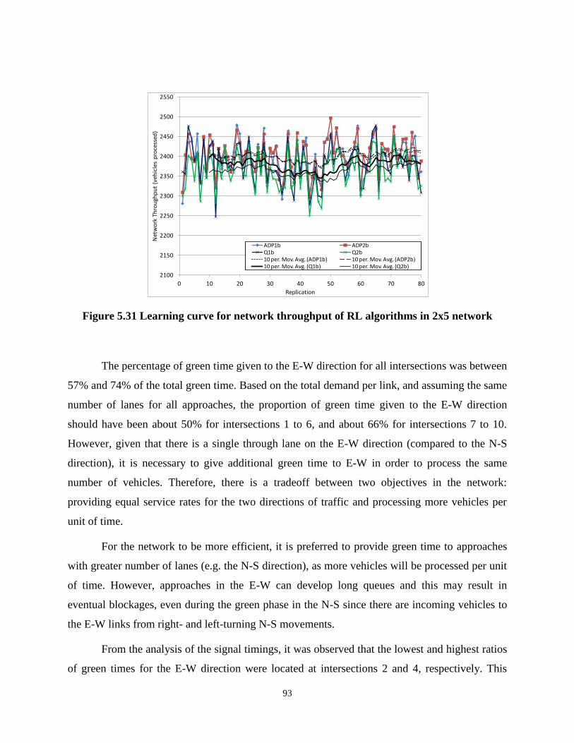
93
Figure 5.31 Learning curve for network throughput of RL algorithms in 2x5 network
The percentage of green time given to the E-W direction for all intersections was between
57% and 74% of the total green time. Based on the total demand per link, and assuming the same
number of lanes for all approaches, the proportion of green time given to the E-W direction
should have been about 50% for intersections 1 to 6, and about 66% for intersections 7 to 10.
However, given that there is a single through lane on the E-W direction (compared to the N-S
direction), it is necessary to give additional green time to E-W in order to process the same
number of vehicles. Therefore, there is a tradeoff between two objectives in the network:
providing equal service rates for the two directions of traffic and processing more vehicles per
unit of time.
For the network to be more efficient, it is preferred to provide green time to approaches
with greater number of lanes (e.g. the N-S direction), as more vehicles will be processed per unit
of time. However, approaches in the E-W can develop long queues and this may result in
eventual blockages, even during the green phase in the N-S since there are incoming vehicles to
the E-W links from right- and left-turning N-S movements.
From the analysis of the signal timings, it was observed that the lowest and highest ratios
of green times for the E-W direction were located at intersections 2 and 4, respectively. This
2100
2150
2200
2250
2300
2350
2400
2450
2500
2550
0 10 20 30 40 50 60 70 80
Net
wo
rk T
hro
ugh
pu
t (v
ehic
les
pro
cess
ed)
Replication
ADP1b ADP2bQ1b Q2b10 per. Mov. Avg. (ADP1b) 10 per. Mov. Avg. (ADP2b)10 per. Mov. Avg. (Q1b) 10 per. Mov. Avg. (Q2b)

94
explains the relatively long queues found in the eastbound direction of intersection 4, as
mentioned above. Incoming vehicles in the eastbound direction entered the link using 74% of the
green time at intersection 2, but only had 57% of the green at intersection 4 to be processed.
On a different performance measure, the average speed of vehicles in the network
improved also in a similar proportion than the delay during the training period (see Figure 5.32).
It is noted that the improvements in the system as training progresses should be observed by
looking at the throughput, delay, and speed simultaneously. In this case delay decreased and
speed increased while maintaining constant throughput (which was equal to the total demand),
but in oversaturated conditions delays may increase and speed decrease while the throughput is
improved.
Figure 5.32 Learning curve for average vehicle speed of RL algorithms in 2x5 network
5.6.3. Summary of Findings
MASTraf implementations with Q-learning and ADP in a 2x5 network with high conflicting
volumes and in undersaturated conditions showed positive results in terms of queue management
and therefore delays and throughput. The demand for this scenario was processed by the agents
as it arrived to the network, thus the system did not increase the saturation level over time. In
addition, the agents showed improvements in performance as the learning process continued with
15
15.5
16
16.5
17
17.5
18
18.5
0 10 20 30 40 50 60 70 80
Ave
rage
Sp
eed
(m
ph)
Replication
ADP1b ADP2bQ1b Q2b10 per. Mov. Avg. (ADP1b) 10 per. Mov. Avg. (ADP2b)10 per. Mov. Avg. (Q1b) 10 per. Mov. Avg. (Q2b)

95
an increased number of replications. Implementations included information regarding potential
blockages in the state and/or in the reward, but in all cases the performance was similar, given
the undersaturated conditions of the system.
5.7. 5x2 Network, Oversaturated Conditions
This section describes the experiments of the 5x2 network from the previous section, but in this
case with oversaturated conditions. A demand of 1000 vphpl was set at all entry points, ensuring
oversaturation and increasing the complexity of the scenario.
5.7.1. Implementation
A key issue in traffic signal control is to prevent blockages in the inner links of the network due
to queue spillbacks. As opposed to single intersections, where oversaturation may create long
queues without reducing the rate at which vehicles are processed, the occurrence of queue
spillbacks and gridlocks in networks can completely prevent the intersections from discharging
vehicles, collapsing the system without recovery. In our reinforcement learning problem, this
also translates to terminal states, from which the agents cannot exit and experience improved
strategies.
In this experiment, two algorithms were tested in oversaturated conditions to illustrate the
need of communication between neighboring intersections. The first implementation used Q-
learning without communication between intersections or any other mechanism to identify
potential blockages downstream (labeled Q1c). A second implementation allowed
communication between neighboring agents and added the potential for blockages to the state
and reward representation (labeled Q2c), similar to the implementation described in the above
section in undersaturated conditions (Q2b).
5.7.2. Performance
The analysis is focused on the total network throughput and queues rather than speed or number
of stops, given the oversaturation. The learning curves for the total network throughput of agents

96
with and without communication are shown in Figure 5.33, where it is observed that the
performance of the agents without communication is significantly lower than with
communication. The number of vehicles processed with communication reached an average of
3870 vehicles processed, which is about 74% of the total demand in all entry links. A more
realistic measure of the efficiency of the network, however, it is necessary by considering that
there are conflicting volumes at entry points and lost time due to yellow-red transitions.
It is estimated that the demand per intersection at entry points is 2000 vphpl. Assuming
that about 1600 vphpl can be processed (with an average discharge headway of 2 seconds and
subtracting about 10% of lost time), the capacity of an intersection should be about 1600 vphpl,
or 80% of the total demand. The total number of vehicles trying to enter the network is 5250,
therefore the capacity should be about 5250*0.8=4200. If this is the case, the network is
currently operating at over 90% efficiency in terms of throughput using the agents with
communication.
Figure 5.33 Learning curve for network throughput of RL algorithms with and without
communication in oversaturated 2x5 network
An examination of the performance of both algorithms showed that the main concern in
this scenario was downstream blockages and gridlocks, often created by left-turning vehicles.
1000
1500
2000
2500
3000
3500
4000
4500
0 20 40 60 80 100 120 140 160 180 200
Net
wo
rk T
hro
ugh
pu
t (v
ehic
les
pro
cess
ed)
Replication
Q1c - No CommunicationQ2c - Communication between agents10 per. Mov. Avg. (Q1c - No Communication)10 per. Mov. Avg. (Q2c - Communication between agents)
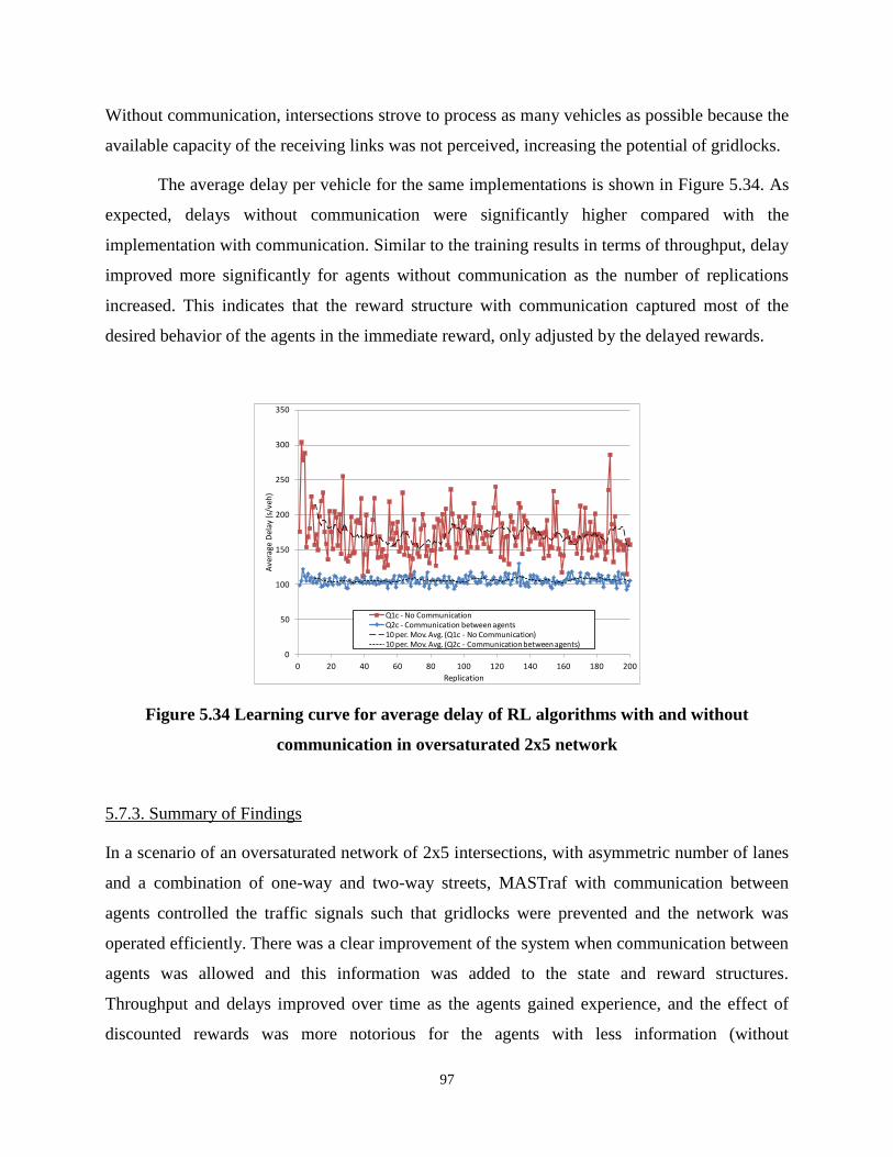
97
Without communication, intersections strove to process as many vehicles as possible because the
available capacity of the receiving links was not perceived, increasing the potential of gridlocks.
The average delay per vehicle for the same implementations is shown in Figure 5.34. As
expected, delays without communication were significantly higher compared with the
implementation with communication. Similar to the training results in terms of throughput, delay
improved more significantly for agents without communication as the number of replications
increased. This indicates that the reward structure with communication captured most of the
desired behavior of the agents in the immediate reward, only adjusted by the delayed rewards.
Figure 5.34 Learning curve for average delay of RL algorithms with and without
communication in oversaturated 2x5 network
5.7.3. Summary of Findings
In a scenario of an oversaturated network of 2x5 intersections, with asymmetric number of lanes
and a combination of one-way and two-way streets, MASTraf with communication between
agents controlled the traffic signals such that gridlocks were prevented and the network was
operated efficiently. There was a clear improvement of the system when communication between
agents was allowed and this information was added to the state and reward structures.
Throughput and delays improved over time as the agents gained experience, and the effect of
discounted rewards was more notorious for the agents with less information (without
0
50
100
150
200
250
300
350
0 20 40 60 80 100 120 140 160 180 200
Ave
rage
Del
ay (s
/veh
)
Replication
Q1c - No CommunicationQ2c - Communication between agents10 per. Mov. Avg. (Q1c - No Communication)10 per. Mov. Avg. (Q2c - Communication between agents)

98
communication), as expected. On the other hand, the state and reward structures captured the
desired behavior of the agents quite accurately, making the learning process less apparent. This
experiment highlights the importance of anticipating blockages in oversaturated conditions, a
feature that in undersaturation did not have a significant impact but that becomes essential with
higher demands.
5.8. 4x5 Network – Q-learning and ADP
This section describes a more complex scenario in a 4x5 network in oversaturated conditions.
The geometry of the network was modeled form a modified version of a portion of downtown
Springfield, IL, and includes one-way and two-way streets in a grid-like configuration. It
comprises the 2x5 network described in the previous two sections, further increasing the
complexity of the signal control task. The network is shown in Figure 5.35.
5.8.1. Implementation
The Q-learning and ADP implementations shared the same state and reward structure and
included information on potential downstream blockages. Therefore, the state representation was
a multidimensional vector describing the queues at the intersection controlled by a given agent,
in addition to indicators of potential downstream blockages, and a dimension for the current state
of the signal.
The reward structure was similar to that described in Chapter 4 for the basic definition of
MASTraf, as a combination of the number of vehicles being served by the green light (with a
positive sign), the number of vehicles waiting to be served in the remaining approaches (with a
negative sign), and a series of penalties (for potential downstream blockages and lost time when
the current phase was changed).

99
Figure 5.35 Schematic representation of the 4x5 network for ADP agents
5.8.2. Performance
Average delay per vehicle, number of trips completed, and network congestion were analyzed
during the training period, as it is shown in Figure 5.36. Note that the range of the vertical axis in
the subfigures is the same for both methods, allowing for easier visual comparisons between
them.
It is observed that there is a wider range of variation in the measures of performance for
the ADP algorithm compared to Q-learning (Figures 5.36(a) and 5.36(b)). While this was not
completely expected, it could be related to the inherent association of states to actions in Q-
learning, which is not present in ADP. Also, in the highly oversaturated conditions tested,
undesirable actions taken by chance or for the sake of exploration may have resulted in
conditions from which it was very difficult to recover (extended queue spillback and blockages).

100
Nevertheless, this was precisely the purpose of the training mode: to gather enough information
for the agent to be able to correctly assess the level of desirability of states/actions when in the
operational mode.
Similar comments also apply to the behavior observed in terms of number of trips
completed (Figures 5.36(c) and 5.36(d)) and the number of vehicles at the end of the simulation
(Figures 5.36(e) and 5.36(f)), where most of the individual runs from ADP in the training mode
yielded less desirable results than Q-learning.
In addition to traffic-related performance measures, the convergence of the Q and V
values was also monitored. For illustration purposes, two sample cases of the evolution of Q and
V values over time are shown in Figure 5.37. In Figure 5.37(a), the convergence is shown for a
state where queues in one direction (E-W) were much higher than for the other (N-S), whereas in
Figure 5.37(b) values are shown for a state where competing demands were the same, which
could present the agent with a more ambiguous situation. However, in both cases the values
either converged or were clearly well ahead in this process, indicating that the algorithms were,
in fact, learning a policy.
It is noted that the solution space for a single agent using Q-learning and ADP was in the
order of 105. However, an analysis of the final Q and V values (after training) showed that only
about 1% to 3% of these states were visited during the training period. Note that this was the
case because the evaluation was performed under a single set of traffic demands. In cases with
variable demand it is expected to visit a significantly higher number of states.
On the other hand, results in the operational mode from Q-learning and ADP were
compared to results obtained using optimized signal timings from the state-of-practice software
TRANSYT7F, based on 30 simulation runs to account for the internal variability of the
simulation software. Then, the same measures of performance described above for the training
mode were analyzed using data from the operational mode, as it is shown in Figure 5.38.

101
Q-learning ADP
a) Average delay per vehicle Q-learning b) Average delay per vehicle ADP
c) Number of trips completed Q-learning d) Number of trips completed ADP
e) Vehicles in network Q-learning f) Vehicles in Network ADP
Figure 5.36 Aggregate results from training stage for Q-learning and ADP
100
120
140
160
180
200
220
0 10 20 30 40 50 60
Ave
rage
De
lay
pe
r V
eh
icle
(s)
Simulation Run
100
120
140
160
180
200
220
0 5 10 15 20 25 30 35
Ave
rage
De
lay
pe
r V
eh
icle
(s)
Simulation Run
3000
3200
3400
3600
3800
4000
4200
4400
4600
4800
5000
0 10 20 30 40 50 60
Trip
s C
om
ple
ted
Simulation Run
3000
3200
3400
3600
3800
4000
4200
4400
4600
4800
5000
0 5 10 15 20 25 30 35
Trip
s C
om
ple
ted
Simulation Run
1000
1100
1200
1300
1400
1500
1600
1700
1800
0 10 20 30 40 50 60
Ve
hic
les
Insi
de
Ne
two
rk a
t en
d o
f Si
mu
lati
on
Simulation Run
1000
1200
1400
1600
1800
0 5 10 15 20 25 30 35
Ve
hic
les
Insi
de
Ne
two
rk a
t en
d o
f Si
mu
lati
on
Simulation Run

102
a) State: Queue EW=7, Queue NS=3, Signal status = green EW
b) State: Queue EW=6, Queue NS=6, Signal status = green EW
Figure 5.37 Convergence of Q and V Values in sample states
Regarding the simulation runs from TRANSYT7F, these were obtained by optimizing the
entire network at the same time and not individual intersections. The procedure in this software
uses a limited version of a genetic algorithm that performs a search in the solution space (signal
timings) with a fix, relatively coarse increment, for example every 10 seconds of cycle length.
All three traffic signal parameters were optimized by TRANSYT7F (cycle, splits, and offsets),
and the measure of performance for the optimization was throughput, given that it was the
measure that more closely related to our reward function.
-1.5
-1
-0.5
0
0.5
1
1.5
2
2.5
0 10 20 30 40 50
De
lta
Q b
etw
ee
n c
on
secu
tive
vis
its
Visits to state-1
-0.8
-0.6
-0.4
-0.2
0
0.2
0.4
0.6
0 20 40 60 80 100
De
lta
V b
etw
ee
n c
on
secu
tive
vis
its
Visits to state
-3
-2
-1
0
1
2
3
4
0 10 20 30 40 50 60 70
De
lta
Q b
etw
ee
n c
on
secu
tive
vis
its
Visits to state-0.3
-0.2
-0.1
0
0.1
0.2
0.3
0.4
0.5
0.6
0 20 40 60 80 100 120 140
Del
ta V
bet
wee
n c
on
secu
tive
vis
its
Visits to state

103
a) Average Delay per Vehicle b) Number of Trips Completed
c) Number of Vehicles inside Network
Figure 5.38 Results from Q-learning, ADP in operational node, and TRANSYT7F
Results from Figure 5.38(a) show that the two algorithms provided a narrower range of
delays concentrated at lower levels than those from TRANSYT7F. Moreover, the average delay
per vehicle from Q-learning (139 s) and ADP (138 s) were significantly lower than the average
delay from TRANSYT7F (159 s) with a 99% confidence level (an improvement of 13%).
Further observation of the simulation runs showed that the main reason for this was that Q-
learning and ADP agents could adapt the signal timings to the small variations in the traffic
100
120
140
160
180
200
220
0 5 10 15 20 25 30 35
Av
era
ge
De
lay
pe
r V
eh
icle
(s)
Simulation Run
Q-learning
ADP
TRANSYT7F
3000
3400
3800
4200
4600
5000
0 5 10 15 20 25 30 35
Trip
s C
om
ple
ted
Simulation Run
Q-learning
ADP
TRANSYT7F
1000
1200
1400
1600
1800
2000
0 5 10 15 20 25 30 35
Ve
hic
les
insi
de
Ne
two
rk a
t E
nd
of
Sim
ula
tio
n
Simulation Run
Q-learning
ADP
TRANSYT7F

104
stream. In some runs, such small variations were able to develop extended queue overflows and
blockages that resulted in significant performance degradation.
Similar observations can be made in terms of system throughput (see Figure 5.38(b)),
were most of the observations from Q-learning and ADP were confined to a narrower range
compared to those from TRANSYT7F. Average number of trips completed for Q-learning
(4718) and ADP (4794) were significantly higher than those from TRANSYT7F (4278) with a
99% confidence level (an improvement of 10%).
Lastly, congestion levels inside the network (Figure 5.38(c)) were similar for Q-learning
and ADP, as expected, but at a lower level than those for TRANSYT7F. This indicates that the
RL algorithms allowed more vehicles inside the network and created longer queues in the inner
links.
5.8.3. Summary of Findings
Experiments in an realistic oversaturated 4x5 network using MASTraf implementations with Q-
learning and ADP showed comparable and improved results compared to a solution found with
TRANSYT7F, reducing average delays by 13% and increasing average throughput by 10% to
12%. The systems accumulated experience as the training period progressed and resulted in
policies that prevented long-lasting queue spillbacks and gridlocks.
These implementations showed that the MASTraf formulation can effectively manage
traffic signals in realistic scenarios both using Q-learning and ADP algorithms. The system is
expected to scale well for larger networks since the complexity of the agent structure does not
increase with the network size.

105
CHAPTER 6 – IMPLEMENTATION OF A STRATEGY FOR SIGNAL
COORDINATION
A shortcoming of a multi-agent system where every agent learns and acts separately is that they
will strive to take actions that maximize their local rewards without considering the global payoff
of the system. For the problem of controlling the traffic signals of a network, agents will take
actions to improve one or a combination of measures of performance such that their own set of
indicators is improved over time. These measures may include throughput, delay, number of
stops, or any other traffic-related indicators.
Traffic networks with high demands may evolve into states that are not able to process
traffic at their capacity due to oversaturation and may create de-facto red and gridlocks. Under
these conditions if agents operate solely on the basis of their approaching links, they may take
decisions that could degrade the performance of adjacent intersections and ultimately their own.
For example, an intersection at the edge of a network may allow vehicles to enter at a rate that is
higher than the rate that can be processed downstream due to high conflicting volumes. This
situation may eventually create queue overflows inside the network and a gridlock, which will
result in a decrease in the throughput at the entry link and for the whole network.
The scenario described above can be encountered when demands are high, and
particularly in situations where conflicting volumes are also high. Therefore, if the traffic system
is controlled by agents operating individual intersections, it is just logical to create means for the
agents to communicate with each other at least to a certain degree.
As mentioned in Chapter 4 when describing the proposed MASTraf, in addition to agents
acting independently, they can also receive information from adjacent intersections and
incorporate it into their perception and decision-making process. This can be achieved in the
form of an extended state representation, changes in the reward structure, experience sharing (Q
values), or a combination of these elements. In turn, information sharing can lead to emergent
coordinated behavior that may favor signal progression along corridors, thereby improving
network performance.
However, information sharing does not explicitly describe a coordination mechanism that
the system designer can incorporate into the agents’ learning process. Therefore, additional

106
complexity can be added to the agent by including explicit coordination between intersections
through the formation of groups and coalitions.
There is extensive research in the areas of group and coalition formation for applications
other than traffic control, and most of the work has been originated from the artificial intelligent
community. More specifically, the focus here is on cooperative agents that share or exchange
some information to achieve better system-wide performance, and where the communication is
achieved in a completely decentralized way.
Communication between agents, without mediation from agents with higher hierarchies,
may allow the formation of (temporary) groups that can improve the overall performance of the
system. For the traffic control domain, it is of outmost importance to maintain acceptable
operational levels in the whole network, since queue spillbacks and traffic breakdowns may
extend to greater areas and ultimately result in system collapse. This research investigates group
formation methods for fully cooperative agents, willing to make decisions that at some point in
time may result in lower individual benefit but achieving higher payoff for the whole system.
Nunez and Oliveira (2003) devised a feature for heterogeneous agents to request advice
from agents with a better performance index, similar to supervised learning. Agents exchanged
their state, the best action for such state (as a means of advice), as well as their performance
index. The effects of the advice exchange were tested using a series of individual intersections
(not along an arterial) in a simple simulator, where each intersection had a different learning
algorithm. Results showed that the advice exchange was likely to improve performance and
robustness, but ill advice was also said to be a problem hindering the learning process.
De Oliveira et al. (2005) used a relationship graph as a support for the decision-making
process. Related agents entered a mediation process to determine the best set of actions. Agents
had priorities and the one with highest value was the leader of the mediation. Branch-and-bound
was performed to find the best outcome of the sub-problem. The test was conducted on a 5x5
network in a very simple simulation environment provided by a generic tool for multi-agent
systems (not a traffic-specific environment). Temporary group formation was achieved and
resulted in improved performance in terms of a cost function, compared to pre-timed coordinated
signals. The agents regrouped (through a new mediation) when traffic patterns changed, adapting
to new conditions.

107
The max-plus algorithm has been used by Vlassis and Kok (2004, 2005, and 2006) and it
emerges as a viable option for controlling the traffic signals in a network. The max-plus
algorithm uses a message-passing strategy that is based on the decomposition of the relations in a
coordination graph as the sum of local terms between two nodes at the time. This allows the
interchange of messages between neighboring intersections, such that in a series of iterations the
agents will reach a final decision based on their own local payoff function as well as the global
payoff of the network.
Kuyer at al. (2008) used coordination graphs and the max-plus algorithm to connect
intersections close to each other. Networks having up to 15 intersections were tested, finding
improved results compared to Wiering (1997) and Bakker (2005). Also, De Oliveira et al. (2004)
have made significant contributions using approaches based on swarm intelligence, where agents
behave like a social insect and the stimuli to select one phase or plan is given by a “pheromone”
trail with an intensity related to the number and duration of vehicles in the link.
A different approach by Junges and Bazzan (2007) studied a strategy using a distributed
constraint optimization problem for networks of up to 9x9 intersections, but only for the task of
changing the offset of the intersections given two different signal plans. A scenario without
online capabilities to change the coordinated direction was compared with the coordinated
scheme, showing improvements in the performance. However, for frequent action evaluations,
and for bigger networks, the methodology may not be practical as the computation time increases
exponentially with the number of agents.
In this research, different from previous approaches, the max-plus algorithm is used to
provide an indication of good coordinating actions, and these results are incorporated to the
reward structure of the agent in the form of an incentive towards the coordinated direction. This
addition to the standard definition of a reward is expected to create a tendency to increase the
system throughput and reduce the number of stops, as it is explored in the sections below.
6.1. The Max-Plus Algorithm
In this research, the max-plus algorithm has been implemented in the reward structure of a Q-
learning agent to determine if it leads to improved performance in an oversaturated network. The

108
max-plus algorithm propagates the combination of local and global payoffs among the agents
that are interconnected in a coordination graph. Locally optimized messages Uij(aj) are sent by
agent i to neighbor j over the edge that connect them and with respect to the action executed by
agent j (aj). For tree structures, the algorithm converges to a fixed point after a finite number of
iterations (Pearl, 1988; Wainwright et al., 2004). However, proof of convergence is not available
for graphs with cycles, and there is no guarantee on the quality of the solution of max-plus in
these cases. Nonetheless, as pointed out in Kok and Vlassis (2006), the algorithm has been
successfully applied in practice in graphs with cycles (Murphy et al., 1999; Crick and Pfeffer,
2003; Yedidia et al., 2003).
A description of the max-plus algorithm is provided in Kok and Vlassis (2006), along
with some considerations for applications on graphs with cycles. For the traffic signal problem
and in particular for grid-like networks, intersections are interrelated by connections in all their
approaches creating a series of cycles between them.
To describe the max-plus algorithm, let’s suppose that the traffic network is a graph with
|V| vertices (or intersections) and |E| edges (or links). To find the optimal action in the network
(a*), agent i repeatedly sends the following message uij to its neighbors j:
(6.1)
Where Γ(i)\j are all neighbors of i except j, and cij is a normalization value. Message uij,
as explained in Kok and Vlassis (2006), is an approximation of the maximum payoff agent i can
achieve with every action of j, and it is calculated as the sum of the payoff functions fi, fij, and all
other incoming messages to agent i, except that from agent j. Messages uij are exchanged until
they converge to a fixed point or until the agents are told to stop the exchange due to an external
signal, for example after the time available to make a decision is over. It is noted that the
messages only depend on the incoming messages of an agent’s neighbors based on their current
actions, thus there is no need to have these messages optimized, nor evaluated over all possible
actions.
On the other hand, the normalization value cij is very useful especially on graphs with
cycles since the value of an outgoing message uij eventually becomes also part of the incoming
ijj\)i(k
ikijiijiia
jij caua,afafmaxauj

109
message for agent i. Thus, in order to prevent messages from growing extremely large, the
average of all values in uik is subtracted using:
(6.2)
In this research, given that the agents are implemented in a microscopic traffic simulator where
the states are updates in a synchronous fashion, a centralized version of the max-plus algorithm
was implemented. The pseudo code of the algorithm is shown in Figure 6.1, following the
implementation described in Kok and Vlassis (2006).
Figure 6.1 Pseudo code of max-plus algorithm, adapted from Kok and Vlassis (2006)
k
kik
k
ij auA
1c

110
6.2. Implementation
The coordinating strategy provided by the max-plus algorithm was implemented along with the
reinforcement learning process in a simulated environment. Therefore, the process to embed
max-plus into the agent structure follows the same procedure described in previous chapters
though the use of the communications interface in the simulator VISSIM and a custom dynamic
linked library (DLL) generated by a C++ code created in this research.
As described earlier, each intersection is operated by a single agent, thus there is a
separate set of state values per agent and they keep track of their own knowledge independently.
Every agent in VISSIM sequentially calls the DLL every simulation second, thus all variables
accessible to the user can be tracked with the same frequency. The current implementation
updates the agents every two seconds, given that this is the typical time needed to process a
single vehicle through an intersection at saturation flow rate. In addition, a 2-second window for
evaluating the next signal response is expected to provide very accurate results, also leaving
more time available to other functions that may be needed, such as communication between
agents and conflict resolution for group formation.
For the experiments, driver behavior parameters from VISSIM have been calibrated to
match the performance of CORSIM with default parameters. This was the case because
performance benchmarks from optimized traffic signals using TRANSYT7F were obtained for
the oversaturated scenario, and this optimizer uses CORSIM as the simulation environment.
The information agents receive about the state of the system is collected via vehicle
detectors placed along the roadway at entry and exit points of all links. This allows for
calculations of the number of vehicles in each link, queues, density, and speeds in all approaches,
which the agents can use to take the control decisions (in addition to information received from
other agents).
Recall that the agents can run the traffic signals with complete flexibility in terms of
timing parameters, thus the operation is not restricted by pre-specified cycle length, splits, or
offsets. Furthermore, restrictions such as maximum green times or phase sequence were not
defined for this implementation, with the exception of a minimum green time of 8 seconds
imposed in all experiments.

111
Implementation of the Q-learning algorithm followed a similar process to that described
by Medina et al. (2010, 2011). The estimation of the goodness of a coordination action from the
max-plus algorithm (functions fi and fij) was based on the state of the links receiving the green
indication. For example, the potential goodness of coordinating intersections 1 and 2 (the two
intersections are adjacent in the E-W direction) will be the sum of their states in the E-W links.
This simple definition will favor coordinated movements based on current states, one pair of
intersections at the time, but eventually for the network as a whole using the max-plus algorithm.
6.3. Simulation Results
A realistic network was used to test the Q-learning and max-plus algorithms. The same network
used in the experiments described at the end of the previous section was also used for the max-
plus evaluation. This is a complex and realistic scenario with 20 intersections in a 4x5 grid-like
configuration and geometry based on a portion of downtown Springfield, IL. There is a
combination of one-way and two-way streets, as well as different number of lanes. Left turns
were allowed from left-turn pockets that had very limited capacity (about 150 feet) and could
block through movements given the high demands (20% of total arriving volume). Also, the left-
turn movements did not have an exclusive signal phase, thus they were only permitted upon
traffic gaps in the oncoming traffic. The network is shown in Figure 5.32 (previous Chapter).
6.3.1. Oversaturation – Heavy traffic in all directions
The algorithms were first tested in a highly oversaturated scenario. Demands ensured severe
congestion in all directions of traffic, with 1000 vphpl at all entry points. The implementation
used Q-learning and included -in the state and reward structures- features to identify potential
blockages and to promote flow of incoming platoons from adjacent intersections. An additional
implementation used the same Q-learning approach structure and also included the results from
the max-plus algorithm in the reward.
The max-plus algorithm quantified the benefits of selecting the green phase for E-W or
N-S direction for each intersection. There are a number of ways to implement these benefits in
the reward and/or in the state representation. As described above, previous studies have used the

112
results of the max-plus algorithm as the major factor to select the phases in a traffic network.
However, it has not been combined with RL strategies to produce a single response to take an
action.
In this case, it was opted to incorporate the results of the max-plus algorithm as a factor
to the immediate reward expected for E-W and N-S actions. The ratio between the max-plus
benefits of E-W and N-S was found and applied as a multiplication factor to the cost of taking
one of the two actions. For example, for a given intersection if the max-plus benefit of selecting
E-W is measured as 10 and the benefit of selecting N-S is 7.5, then the reward value of E-W is
increased by a factor of 10/7.5=1.33, and the value of N-S is not modified.
Using this procedure the max-plus results were incorporated into the RL decision-making
process, promoting the actions toward improved coordination.
The performances of the agents with and without max-plus are analyzed along with the
performance optimized signal timings from TRANSYT7F.
The total network throughput for the MASTraf implementations and TRANSYT7F is
shown in Figure 6.2. It can be observed that the throughput using Q-learning in the first stages of
the learning is lower than the one found by TRANSYT7F, but as the learning goes on there was
a tendency to produce a greater number of vehicles processed. Also, the learning with max-plus
had a steeper incline in the early replications compared to the Q-learning algorithm without the
coordinating mechanism.
Figure 6.2 Network throughput TRANSYT7F and Q-learning, oversaturated conditions
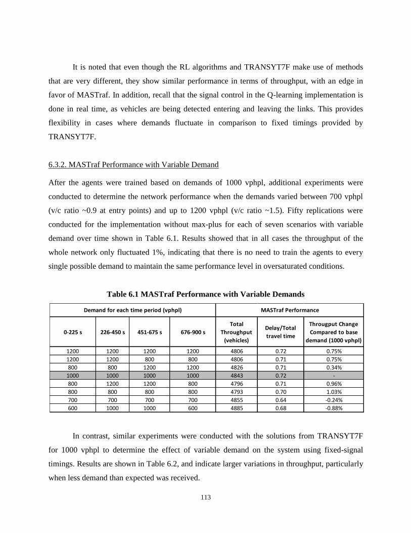
113
It is noted that even though the RL algorithms and TRANSYT7F make use of methods
that are very different, they show similar performance in terms of throughput, with an edge in
favor of MASTraf. In addition, recall that the signal control in the Q-learning implementation is
done in real time, as vehicles are being detected entering and leaving the links. This provides
flexibility in cases where demands fluctuate in comparison to fixed timings provided by
TRANSYT7F.
6.3.2. MASTraf Performance with Variable Demand
After the agents were trained based on demands of 1000 vphpl, additional experiments were
conducted to determine the network performance when the demands varied between 700 vphpl
(v/c ratio ~0.9 at entry points) and up to 1200 vphpl (v/c ratio ~1.5). Fifty replications were
conducted for the implementation without max-plus for each of seven scenarios with variable
demand over time shown in Table 6.1. Results showed that in all cases the throughput of the
whole network only fluctuated 1%, indicating that there is no need to train the agents to every
single possible demand to maintain the same performance level in oversaturated conditions.
Table 6.1 MASTraf Performance with Variable Demands
In contrast, similar experiments were conducted with the solutions from TRANSYT7F
for 1000 vphpl to determine the effect of variable demand on the system using fixed-signal
timings. Results are shown in Table 6.2, and indicate larger variations in throughput, particularly
when less demand than expected was received.
0-225 s 226-450 s 451-675 s 676-900 s
Total
Throughput
(vehicles)
Delay/Total
travel time
Througput Change
Compared to base
demand (1000 vphpl)
1200 1200 1200 1200 4806 0.72 0.75%
1200 1200 800 800 4806 0.71 0.75%
800 800 1200 1200 4826 0.71 0.34%
1000 1000 1000 1000 4843 0.72 -
800 1200 1200 800 4796 0.71 0.96%
800 800 800 800 4793 0.70 1.03%
700 700 700 700 4855 0.64 -0.24%
600 1000 1000 600 4885 0.68 -0.88%
Demand for each time period (vphpl) MASTraf Performance

114
Table 6.2 TRANSY7F Performance with Variable Demands
6.3.3. MASTraf Performance with Imprecise Detector Data
Additional runs were conducted to determine the system response when the information received
from vehicle detectors was imprecise. Scenarios for the oversaturated network of 4x5
intersections with data from detectors aggregated at different levels were compared to the initial
implementation where up to 20 states were possible for each phase. Recall that links may store
significantly higher number of vehicles than 20, thus with the standard application some
resolution was already lost.
Agents were trained with detector data that was more aggregated than in the initial
implementation. Data was aggregated by scaling down the number of possible states for a given
phase. Coarser aggregation (or reduced resolution) levels created imprecision in the information
received by the agents since an increasing number of vehicles were represented by the same
state. For example, at 25% resolution, a coarser representation with only 5 possible states for a
phase was sent to the agent, instead of having 20 possible states. Imprecision may translate to
inaccuracies in green time allocation and prevention of upstream blockages.
The following resolution levels were tested in separate experiments: 90% resolution (up
to 18 states), 75% resolution (up to 15 states), 50% resolution (up to 10 states), and 25%
resolution (up to 5 states). The effects of coarser detector data were measured in terms of
network throughput and average number of stops per vehicle. For each resolution level, the
training was conducted over 120 realizations of 15 minutes each, and the analysis was based on
30 repetitions obtained after the training runs were completed.
0-225 s 226-450 s 451-675 s 676-900 s
Total
Throughput
(vehicles)
Delay/Total
travel time
Througput Change
Compared to base
demand (1000 vphpl)
1200 1200 1200 1200 4706 0.75 2.83%
1200 1200 800 800 4704 0.75 2.86%
800 800 1200 1200 4728 0.72 2.38%
1000 1000 1000 1000 4769 0.75 -
800 1200 1200 800 4718 0.73 2.58%
800 800 800 800 4724 0.71 2.45%
700 700 700 700 4539 0.61 6.28%
Demand for each time period (vphpl) TRANSYT7F Performance

115
Results for all resolutions are shown in Figure 6.3. The reduction in detector resolution
produced limited effects both in terms of throughput and number of stops, especially with 90%
and 75% of the initial resolution. MASTraf managed to continue processing vehicles in
oversaturated conditions, although on average the total network throughput and stops per vehicle
were affected as shown in Figure 6.3.
Lower resolution levels (50% and 25%) further lowered MASTraf efficiency. At low
detector resolution the system performance also becomes less stable and the variation in the
measures of performance increase significantly, as seen in the two wider ellipses in Figure 6.3.
However, notice that even with very coarse approximations the system prevented the network
from collapsing.
Figure 6.3 Effect of lower detector resolution on network throughput and stops per vehicle
6.3.4. Extending the State Representation for Coordination
The performance of the Q-learning implementation was also examined when the max-plus was
added to the reward structure. Two cases were explored: One with an augmented state
representation indicating if the coordinated direction was E-W or N-S (using a binary variable),
4.5
4.7
4.9
5.1
5.3
5.5
5.7
4000 4200 4400 4600 4800 5000 5200
Ave
rage
Nu
mb
er
of
Sto
ps
pe
r V
eh
icle
Average Network Throughput
Standard resolution (100%)
90% resolution
75% resolution
50% resolution
25% resolution
Ellipses indicate plus and minus one standard deviation from the average value

116
and one without augmenting the state. Figure 6.4 shows the results for the two applications of the
max-plus together with the application without the coordinating algorithm, in terms of number of
stops per vehicle and throughput. Oversized symbols in Figure 6.4 show the average values for
each of the series.
Figure 6.4 Q-learning with and without max-plus, oversaturated conditions
From Figure 6.4, the use of the max-plus algorithm without the extended state resulted in
increased average throughput and reduced average number of stops. However, adding
information on the coordinating direction to the state did not result in significant improvements.
This could be case due to the nature of the max-plus implementation itself, where
multidirectional coordination may result between neighboring intersections, promoting
immediate localized benefits but not necessarily network-wide improvements at the end of the
time period.
6.3.5. Light Traffic Conditions – Heavier traffic in one direction
An additional scenario explored the effects of the max-plus algorithm in light traffic conditions
with higher demands in the N-S direction. The 4x5 network from previous experiments was also
4
4.5
5
5.5
6
6.5
7
4300 4500 4700 4900 5100
Ave
rage
Sto
ps
pe
r V
eh
icle
Throughput
Q-learning WITHOUT Max-plus
Q-learning WITH Max-plus
Q-Learning WITH Max-plus and Extended State

117
used in this case. Demands were ¼ of the saturation level volumes in the E-W direction (250
vphpl), and ½ of the saturation levels in the N-S direction (vphpl).
Simulation runs were conducted with and without max-plus to determine if the algorithm
affected the traffic operation in undersaturated conditions, either positively or negatively. Results
are based on a total of 150 runs for each condition (with and without max-plus), which include
the first 120 runs as the agents’ training period and the last 30 runs for estimating final measures
of performance.
Results showed that in light traffic conditions, the addition of max-plus did not have any
significant effects in the total network throughput. As expected, the total demand was processed
by the agents and there was no change in the number of vehicles in the network over time,
showing no increase in congestion. Out of the total demand expected in all entry links together
during the 15-minute evaluation period (2750 vehicles), the average network throughput without
max-plus was 2723 vehicles, and with max-plus it was 2722 vehicles.
Regarding the number of stops per vehicle, results indicate no significant change at the
network level due to the addition of the max-plus algorithm. Average number of stops per
vehicle using MASTraf and without max-plus were already low at 1.13 stops for the whole
network combined. This number did not change to the second decimal place when max-plus was
used.
These results indicate that the addition of max-plus to MASTraf did not improve
significantly the operation in undersaturated conditions and at the same time did not impact the
operation negatively. Moreover, it may be acceptable to operate MASTraf with max-plus in both
undersaturated and oversaturated conditions, as the algorithm does not have negative
implications in light traffic, but it may improve performance as traffic congestion increases.
6.3.6. Congested Conditions – Heavier traffic in one direction
A third scenario was also examined, where the demands were high, asymmetric and heavier in
one direction of traffic in the whole network. The objective of this experiment was to determine
if under dominant loads in one direction, the max-plus algorithm could provide improvements in
the performance of the RL implementation. Two scenarios: with and without max-plus were
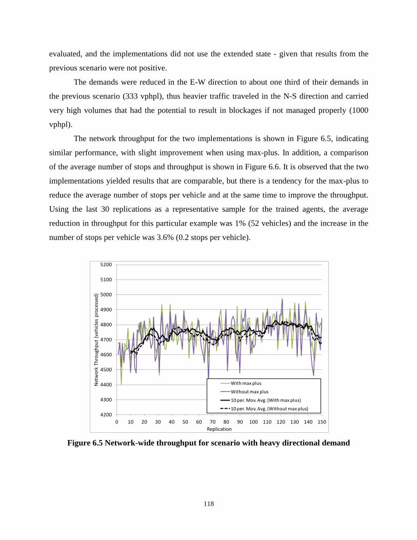
118
evaluated, and the implementations did not use the extended state - given that results from the
previous scenario were not positive.
The demands were reduced in the E-W direction to about one third of their demands in
the previous scenario (333 vphpl), thus heavier traffic traveled in the N-S direction and carried
very high volumes that had the potential to result in blockages if not managed properly (1000
vphpl).
The network throughput for the two implementations is shown in Figure 6.5, indicating
similar performance, with slight improvement when using max-plus. In addition, a comparison
of the average number of stops and throughput is shown in Figure 6.6. It is observed that the two
implementations yielded results that are comparable, but there is a tendency for the max-plus to
reduce the average number of stops per vehicle and at the same time to improve the throughput.
Using the last 30 replications as a representative sample for the trained agents, the average
reduction in throughput for this particular example was 1% (52 vehicles) and the increase in the
number of stops per vehicle was 3.6% (0.2 stops per vehicle).
Figure 6.5 Network-wide throughput for scenario with heavy directional demand
4200
4300
4400
4500
4600
4700
4800
4900
5000
5100
5200
0 10 20 30 40 50 60 70 80 90 100 110 120 130 140 150
Net
wo
rk T
hro
ugh
pu
t (v
ehic
les
pro
cess
ed)
Replication
With max plus
Without max plus
10 per. Mov. Avg. (With max plus)
10 per. Mov. Avg. (Without max plus)

119
Figure 6.6 Q-learning with and without max-plus directional demand
6.4. Summary of Findings
In summary, results presented in this paper shows that RL agents can efficiently control the
traffic signals of a realistic network in real time in conditions that are challenging for traditional
and more complex traffic control systems, including oversaturation with fixed and variable
demand. Oversaturation is especially challenging for independent agents, but results indicated
that even in this conditions the traffic signals prevented spillbacks and gridlocks and at a level
comparable or better than state-of-practice traffic optimization software.
Communication between agents was not only used to inform neighboring agents of
potential downstream blockages, but also to create a coordinating mechanism using the max-plus
algorithm. The coordinating mechanism acted as a bias to the reward function, favoring actions
with improved coordination. The max-plus algorithm was set to respond to local link demands at
each intersection, and yielded improved average results both in terms of total throughput and
number of stops per vehicle.

120
CHAPTER 7 – IMPLEMENTATION OF A VALUE FUNCTION APPROXIMATION
Different forms of reinforcement learning, and specifically the original formulations of Q-
learning and the approximate dynamic programming (ADP) algorithms used in this research,
make use of lookup tables to store an agent’s past experience and knowledge. While tables have
the advantage of recording precise information on experiences from every single state that has
been visited, it is expensive in terms of storage requirements and it doesn’t generalize past
experiences to similar states.
Alternatives have been proposed to store an agent’s knowledge using structures different
from lookup tables. A common approach is the use of other structures or a series of functions to
model the change of an agent’s perception of reward in a more compact fashion. These
techniques will be referred in this research as function approximation methods.
Before elaborating on the approach adopted in this study to implement a function
approximation, it is appropriate to first motivate its use by describing some potential benefits. As
expected, the advantages of using function approximation mainly aim at counteracting the
limitations of lookup tables mentioned above: storage requirements and generalization. Storage
requirements are reduced by having a more compact representation of the agent’s knowledge and
the magnitude of these reductions depend on the number of functions and features included in a
given implementation. On one end, if all elements perceived by the agents (and included in the
state) are incorporated in the same number of functions, a great number of parameters will be
required and the reduction in storage requirements may not be as critical as expected. However,
if the number of functions is reduced and the elements can be combined efficiently, the storage
allocation will be a major benefit achieved with a function approximation.
In addition to lessen storage requirements, function approximation also provides a
generalization of the lookup table that is useful to obtain information about states that have not
been visited or those from which not enough experience has been gathered. This is because it is
often the case that states with similar characteristics will tend to produce similar Q or V values in
the lookup tables, with the exception of boundaries or discontinuities.

121
In particular, for our traffic signal problem, features to be used in a function
approximation could be related to current traffic demands, queues, delays or any other feature to
which the agent has access in order to estimate the state values (or discounted rewards).
Therefore, it may be convenient to include in the functions a set of features with impact on the
state and reward definitions, and moreover, those features having a significant role in the
estimation of Q or V values if a lookup table were used.
The combination of features to approximate the lookup table may include linear or non-
linear regressions methods, decision trees, and often in practice, artificial neural networks to
model complex interactions. It is recognized, however, that simple solutions may be preferred
over complex ones, and the exploration of linear regressions should precede more elaborated
methods.
General approaches to produce a more compact state or action representation through
function approximation have recently been summarized for the robot reinforcement learning
domain by Kober and Peters ( 2012) into: neural networks (multi-layer perceptrons, fuzzy neural
networks, and explanation-based neural networks), generalization from neighboring cells, local
models through regression, and Gaussian model regression.
Earlier work by Mahavedan and Connell (1991) proposed basic but key ideas for
generalization of the state space from neighboring cells through the use of the Hamming
distance, a measure to determine how different states are based on the number of bits that are
different between them. This form of generalization significantly sped up the learning process
but it was dependent on the state encoding. Further refinements also by the same authors featured
statistical clustering for generalization, which reduced coding limitations of the Hamming
distance by grouping states based on the effect that an action will have on them. Generalization
with Hamming distance improved learning time of standard Q-learning with lookup tables, and it
was further improved by implementing the statistical clustering for the domain of a mobile robot.
Neural network applications opened their way into reinforcement learning with research
by Barto and Anandan (1985). Implementations for decisions between multiple actions (not only
two possible actions) have been proposed by past research, perhaps being the QCON proposed
by Lin (1993) one of the earliest ones, with the drawback of having as many networks as the
number of possible actions the agent can take. This is circumvented, as shown by Mahadevan

122
(1991) by modifying the network structure and having one output neuron for each action set,
where sets are ‘antagonists’ or play opposed roles for the agent.
Neural networks have been used since in a very wide range of applications, including
traffic signal control. A series of approaches have been proposed, from completely centralized to
partially and fully decentralized. Research by Bingham (1998, 2001) in traffic signal control
using fuzzy rules and a neural network, Abdulhai (2003) using a Cerebellar Model Articulation
Controller (CMAC), Choy et al. (2003) with hierarchical agents and a neural network, and Xie
(2007) and Zhang (2007), are examples in this domain.
On the other hand, Irodova and Sloan (2005) described examples of earlier research on
function approximation for model-free reinforcement learning, such as Q-learning and ADP.
They cite the formulations by Stone and Veloso (1999) using a function approximation for a
multi-agent system based on action-dependent features to partition the state space into regions,
and the seminal book by Russel and Norvig (2003) “Artificial Intelligence, a Modern Approach”.
The work conducted by Irodova and Sloan followed a different approach using a linear
approximation, and is important to the research presented in this document since this was the
approach adopted for a function approximation exercise using MASTraf.
To illustrate the results of implementing a linear function approximation on one of the
MASTraf definitions tested in this research, the Q-learning implementation used in the
oversaturated 4x5 network described in a previous section will be used as an example, as
follows.
7.1. Implementation
A linear function approximation using elements from the state (and also the reward function) was
implemented following an approach based on the same learning process used for the Q-values in
the lookup tables.
Therefore, a similar update rule was applied to the multipliers accompanying the selected
features from the state representation. A previous work from Idorova and Sloan (2005) has been
used as a reference for the formulation of the learning process in the linear function
approximation. For a Q-learning agent, element-based actions are identified and a Q function is

123
created for each of such actions, which in turn include a set of multipliers that will be trained
based on the agent’s experience. Thus, a generic Q function for a given action (a) could be
expressed as follows:
(7.1)
Where f1, ..., fn are the features or elements representative of the state and cost, and θa1 are the
multipliers. For such Qa functions, multipliers θa1 will be updated following a standard Q-value
algorithm but with respect to the particular slope for each θa1, as follows:
𝜃𝑘𝑎(𝑠, 𝑎) = (𝑐𝑠𝑠′
𝑎 + 𝛾 max𝑎′
𝑄(𝑠 ′, 𝑎′))𝑑𝑄𝑎(𝑠,𝑎)
𝑑𝜃𝑘𝑎 (7.2)
and,
𝜃𝑘𝑎(𝑠, 𝑎) = (1 − 𝛼)𝜃𝑘
𝑎(𝑠, 𝑎)𝑑𝑄𝑎(𝑠,𝑎)
𝑑𝜃𝑘𝑎 + 𝛼𝜃𝑘
𝑎(𝑠, 𝑎) (7.3)
Where �̂�𝑎(𝑠, 𝑎) is the current estimation of the value of the state-action pair, which is later
weighted along with the past accumulated knowledge 𝑄(𝑠, 𝑎). 𝑑𝑄𝑎(𝑠,𝑎)
𝑑𝜃𝑘𝑎 is the partial derivative
of the value of the state-action pair with respect to the current multiplier θak for action a.
Similar to the lookup table representation for standard Q-learning, the expression for the
function approximation is completely decentralized and does not increase in size as the number
of intersections increases.
The selection of the features to be included in the function approximation, and the
number of functions to be estimated were determined from the original definition of the reward
structure used in previous experiments with successful results in the oversaturated 4x5 network.
Thus, continuous rewards along a range of values from previous implementations were
identified, as well as the discontinuities due to penalties. More specifically, the discontinuities
were created by the indication of potential blockages in downstream links and the lost time due
to the phase change.
In the reward function from the lookup table implementation the potential for blockages
(P1) was penalized using the following expression:
nan1
a1
a f...fa,sQ

124
(7.4)
Where 𝛽𝐷𝑖𝑟(𝑎) is a scaling factor for a given direction of traffic that will be selected by an action
a, set to 1 in this case; 𝑆𝐷𝑖𝑟(𝑎)2 is the square of the value of the state component in the direction
potential blockage is expected; and 𝑏𝐷𝑖𝑟(𝑎)𝑑𝑜𝑤𝑛 is the blockage factor (or blockage intensity) in the
immediate downstream intersection in the same direction of traffic, which is also reflected in the
state space as a separate dimension.
Penalty P1 will only be in effect whenever there is potential for blockage in any of the
immediate downstream intersection, and therefore will create a discontinuity in the reward
function in such cases. Given that only two directions of traffic are considered in the network,
three cases are considered: blockage in the current direction of traffic only, blockage in the two
directions of traffic, and no blockages. It is noted that for a given action the case of blockage
only in the opposing direction of traffic was not considered since it will affect the reward of the
opposing action.
In addition to this penalty, agents incurred in a second penalty (P2) due to lost time when
the signal phase is changed. This penalty was not always present in the reward function and
therefore it creates a discontinuity for some of the states. The value of the penalty decreased with
the phase duration, representing the greater percentage of the cycle time that is lost if phases are
changed often. The form of the penalty function is:
(7.5)
Where 𝑡𝑃ℎ𝑎𝑠𝑒 is the time that has elapsed since the beginning of the current phase (to be
finished by action a), 𝛽/𝐷𝑖𝑟(𝑎) is a scaling factor for the direction of traffic currently receiving
green (opposed to direction a), and 𝑆/𝐷𝑖𝑟(𝑎) is the state of such direction.
The combination of these two discontinuities due to penalties resulted in a total of six
functions to be approximated: 3 levels of blockages x 2 levels of phase changes (one per action).
Each of these functions had their own set of θa (for a given action a), which were
calibrated through the updating process described above as the agents trained. The action
features selected for the function approximation were the state of the two directions of traffic at a
down)a(Dir
2)a(Dir)a(Dir1 b*S*)a(P
)a(Dir/)a(Dir/
Phase
Phase2 S**
5.0t
12t*2)a(P

125
given time (𝑆𝐸𝑊 and 𝑆𝑁𝑆) and the current phase duration (𝑡𝑃ℎ𝑎𝑠𝑒). This indicates that a total of
three sets of thetas had to be estimated for each of the six functions, for a total of 18 parameters
in the function approximation problem for a given action.
7.2. Performance
Experiments were conducted to determine the performance of the agents with and without state-
action approximations using the linear approach described above. The scenario selected for these
experiments was the 4x5 network used in previous chapters under constant oversaturated
conditions, with demands at all entry links of 1000 vphpl.
Agents using the function approximation were trained following the same procedure
applied for the runs previously obtained for the oversaturated scenario with agents and lookup
tables. The performance of the network for the two implementations in terms of network
throughput as the agents trained is shown in Figure 7.1.
Figure 7.1 Network throughput for MASTraf with and without function approximation
3800
4000
4200
4400
4600
4800
5000
5200
0 10 20 30 40 50 60 70 80 90 100 110 120 130 140 150
Net
wo
rk T
hro
ugh
pu
t (v
ehic
les
pro
cess
ed)
Replication
Q-learning Function Approximation
Q-learning Lookup Table
10 per. Mov. Avg. (Q-learning Function Approximation)
10 per. Mov. Avg. (Q-learning Lookup Table)

126
From Figure 7.1, agents storing their knowledge using a function approximation
converged to a given throughput level very rapidly, given the number of parameters to be
calibrated (a total of 18 thetas per agent). However, the performance at the end of the training
period was lower than that of the agents updating a full lookup table. These results were
expected and also agree with results from previous research running simple function
approximation methods. The reduction in the average network throughput for the last 50
replications (when agents can were trained) with the function approximation was in the order of
1% of the total, thus this approach may be worth to be considered when training time or samples
are limited, and in cases when rapid convergence is desired (e.g. field deployments with limited
simulation training).
Regarding the spread of the exploration in the state space, the percentage of states visited
out of all possible combination of states was very low and in the order of 1%. However, this
could be attributed to combinations that are not practically observable, continuous oversaturation
levels (preventing instances with low link occupancy), and the fast convergence of the functions
given the low number of parameters. In comparison, it is recalled that only 1% to 3% of all
possible states were also visited during training in the lookup table implementations.
Following the same format as in previous sections, the average number of stops versus
throughput were plotted for the last 50 replications of the training period. Here the difference in
the performance between the two implementations is more evident, but in total the average
number of stops per vehicle only increased by 3% with the use of the function approximation.
An examination of the network performance in terms of the total congestion in the inner
links at the end of the simulation period showed that agents running the function approximation
generated lower delays for those vehicles already in the network, indicating that more vehicles
were left outside of the network by having shorter cycle lengths and greater lost times. This also
resulted in lower delays for the vehicles inside the network at the expense of those outside of the
network boundaries in the implementation running the function approximation.

127
Figure 7.2 Number of stops and throughput for MASTraf with and without function
approximation
7.3. Policies
Policies found by the agents with the function approximation were further analyzed to determine
if the behavior of the traffic signals at the level of a single intersection was as expected. Policies
were found after the parameters of the function approximation had converged through training.
The parameters (θan) were used to determine the expected value of the state assuming that the
agent commits to an action, as shown in Equation 7.1. Then, the state values of the two actions
were compared and the highest expected reward determined the agent’s action of choice
assuming a greedy behavior.
Given that there are multiple dimensions in the state representation, it is difficult to
visualize the change of state values using all variables. Therefore, only cases without blockages
and for a given phase duration were analyzed at once.
The planes for each of the two functions that determine the state values (one per action)
were overlapped to determine the intersecting line. The intersection indicates the points at which
4
4.5
5
5.5
6
6.5
7
4200 4400 4600 4800 5000 5200
Ave
rage
Sto
ps
per
Veh
icle
Throughput
Q-learning Look-up table
Q-learning Function Approximation

128
the agent may change its decision. Once this line was determined, the policies given the E-W and
N-S states could be directly observed in terms of the action selection.
An example of the changes in the state values for each action at intersection number 16 in
the 4x5 network illustrated in Figure 5.35 is shown below in Figure 7.3. This example assumes
that at the moment of the analysis the green indication was displayed on the E-W direction, there
were no blockages, and the phase duration was 10 seconds. Intersection 16 has two-way streets
with a single lane for the E-W directions and two lanes in the N-S direction.
In Figure 7.3, the state values are provided for different combinations of E-W and N-S
states. The current signal status is important because if the agent decides to change the phase,
there will be lost time and therefore a reduction in the state value. In a greedy action selection
policy the agent will select the action with higher expected value, thus the intersection of these
two scatter plots (after the plots were approximated to surfaces) was found and it is shown in
Figure 7.4.
A better visualization of the agent policy, instead of the value of the states, can be plotted
by indicating the action selection given the state on the E-W and the N-S directions. Essentially,
the procedure simply requires subtracting the two surfaces and finding the positive and negative
regions, which represent the agent decision on next phase. Thus, if the subtraction is completed
as value(E-W) – value (N-S), positive values will indicate that the agent would choose giving
green to the E-W direction and negative values would indicate that agent choice is the N-S
direction instead.

129
(a)Value of changing the phase to N-S
(b)Value of continuing the phase in E-W
Figure 7.3 Value of states for Intersection 16

130
Figure 7.4 Expected state values for competing actions in intersection 16 without blockages
The results of this process for intersection 16 are shown in Figure 7.5, for the case when
the green indication is currently on the E-W direction (Figure 7.5(a)), and also for the case when
green is currently on the N-S direction (Figure 7.5(b)). Notice that the phase duration is also
important since the planes from Figures 7.3 and 7.4, and therefore Figure 7.5, are a function of
this variable. The effect of phase duration in the policy will be further described in the next
section.
The range of values in Figure 7.5 for the E-W and N-S states only show the combinations
that were often experienced by the agent and not the whole set of possible state values (from 0 to
19). This indicates that combinations such as E-W state=15 and N-S state=18 were not observed.
The range of values also shows that the N-S approaches stored more vehicles than the E-W. This
is expected given the difference in the number of lanes and also because the signal operation was
based mainly on queue management, not on actual number of vehicles at the signal. The agent
objective is to process vehicles and prevent queue backups and blockages, thus maintaining
similar-sized queues could be a valid policy.

131
(a) Policy when E-W is receiving green time (b) Policy when N-S is receiving green time
Figure 7.5 Agent policy at intersection 16 when green is given to any of the two approaches
From Figure 7.5, it is noted that at intersection 16 there is a tendency to continue
displaying the green indication on the approach that currently has the right of way. This is
reflected by the greater surface covered by the actions maintaining the current green phase
(Figures 7.5(a) and 7.5(b)). This result is also expected given the penalty for lost time.
In general, policies at intersection 16 follows expected behavior because the agent would
continue the current phase if the state value remains high, and select the opposite action if the
state for the competing demands is high and the current is low. Furthermore, a bias towards
selecting the phase currently displayed gives an indication of the effects of the lost time
parameter (Equation 7.5) in the reward structure.
In addition to the policies for intersection 16, other intersections in the network were
analyzed to determine if similar policies resulted at locations with different number of lanes and
traffic patterns. One of the selected locations was intersection 1 (see Figure 5.35), which had two
one-way streets, each street with three through lanes.
The policies for intersection 1 are shown in Figure 7.6, and indicate similar trends to
those observed for intersection 16. There is preference to continue the green indication in the
direction that currently has it, unless the difference in the states is large enough to switch phases
and justify the lost time. From the range of values, it is also observed that more vehicles were
Give Green to N-S
Continue Green on E-W
Continue Green on N-S
Give Green to E-W

132
queued in the N-S direction compared to the E-W direction. This is because the N-S approach
was directly located at an entry points, whereas the E-W approach was next to an exit link. The
number of vehicles in the N-S link grows faster and more uniformly than on E-W, but it is
possible that the N-S traffic could not always be processed due to possible downstream
restrictions. The E-W link, on the other hand, could always go through the intersection since the
receiving link was an exit.
The surface on Figure 7.6(a) follows a-priori expectations by not terminating the E-W
phase (processing vehicles towards the exit) unless a significant number of vehicles build enough
pressure to enter the network.
A third intersection, with different geometry, was also explored to determine the agent
policy. At intersection 8 (see Figure 5.35) there were three lanes in the N-S direction at an entry
point, and only one crossing lane per direction on the E-W direction. The agent policies are
shown in Figure 7.7, where it is noticed that there is more pressure to provide green to N-S than
to E-W even in cases where the current signal is in the E-W direction. This also follows
expectation given the difference in number of lanes and volumes between competing links.
(a)Agent policy when green is given to E-W (b) Agent policy when green is given to N-S
Figure 7.6 Agent policy at intersection 1 when green is given to any of the two approaches
Continue Green on E-W
Give Green to N-S
Give Green to E-W
Continue Green on N-S

133
(a)Agent policy when green is given to E-W (b) Agent policy when green is given to N-S
Figure 7.7 Agent policy at intersection 8 when green is given to any of the two approaches
In addition to the policies for fixed phase duration, the change in the decision-making
surface was also analyzed for a case when the phase duration varied. This is shown for
intersection 8 in Figure 7.8.
As the phase duration increased, the agent’s actions also shifted. The policy behavior
shows that opportunities to change the current phase were reduced as the phase duration
increased. For example, if the green signal is currently assigned to the N-S direction and the
phase duration is increasing, there are a decreasing number of combinations of E-W and N-S
states that would result in the agent changing the green phase to E-W. However, the combination
of states that could result in a phase change are very likely and include higher accumulating
demands in the E-W direction and lower discharging demands in the N-S direction.
Continue Green on E-W
Give Green to N-S
Give Green to E-W
Continue Green on N-S

134
(a)Phase duration = 5 s (b)Phase duration = 10 s (c)Phase duration = 20 s
Figure 7.8 Changes in policy when phase duration increases in Intersection 8
7.4. Summary of Findings
A linear function approximation was implemented to generate a more compact representation of
the state using a Q-learning algorithm and the structure provided by MASTraf. A complex
scenario was selected for this exercise, with a 4x5 realistic network in oversaturated conditions.
Results indicate that a simple linear approximation of the Q values was effective for the
fully decentralized system proposed in this research, accounting for discontinuities generated by
penalties in the reward structured only experienced by the agents when there was potential for
blockage due to downstream congestion and due to lost times when a phase was terminated.
Performance in terms of network throughput and number of stops showed for this
exercise that the function approximation resulted in 1% reduction in the total network throughput
and about 3% increase in the number of stops. Therefore, simple approximations such as the one
performed in this section is suitable for systems where these performance drops are acceptable
and also in cases where fast convergence is needed, as the number of iterations to estimate the
reduced number of parameters to be calibrated.
Policies generated by the agents using the function approximation indicated that the agent
behavior followed expected trends, with phase assignments that were proportional to the state in
the two competing traffic directions and the phase duration.

135
CHAPTER 8 –STRENGTHS, LIMITATIONS, FUTURE EXTENSIONS, AND
POTENTIAL FOR FIELD IMPLEMENTATIONS
8.1. Strengths
Experimental results from MASTraf have showed that the proposed system has potential to
efficiently manage the signals in undersaturated and oversaturated networks. Moreover, analyses
of the agents’ performance indicate that a learning process was in fact taking place during the
training period, leading to a policy that improved over time.
The agents’ structure in MASTraf was formulated taking into account traffic engineering
concepts as the first priority. Then, the application of the techniques from machine learning and
the skills to complete the implementation in the simulation software followed the process to
create the agents. Being developed from the traffic engineering point of view is one of the main
differences and strengths of MASTraf compared to previous tools for managing traffic signals in
networks.
A number of characteristics were considered necessary for MASTraf to be properly
designed and tested under different scenarios. These characteristics can be summarized into two
categories: 1) the agent and system definition, and 2) the simulation environment for testing. In
the first category, agents were provided with elements to recognize conditions to manage queues,
generate coordination, and efficiently use green time splits. Communication between agents was
recognized to be important mostly in oversaturated conditions, preventing queue spillbacks and
gridlocks. On the simulation environment, a widely accepted simulator was chosen for the
testing performed on MASTraf in order to assure that well known variations in traffic behavior
were taken into account. The use of a commercial simulator also may give more confidence to
the testing results in the traffic engineering community, given that the agents experience
situations with complexities similar to those in the field.
In comparison to other implementations, MASTraf combines features implemented in a
fully decentralized fashion, with capabilities to operate in undersaturated and oversaturated

136
conditions. Communication between agents is allowed to implement these features, not only by
means of information passing, but also for an explicit coordinating strategy, such as the max-plus
algorithm used in this research.
Experiments have also shown that current MASTraf formulation responded positively to
variations in the expected traffic demands, thus reducing requirements of training under every
possible condition that can be experienced in the field. MASTraf reliance on detectors was also
tested
Dynamic group formation is also considered as an important feature of MASTraf and was
implemented as a bias in the reward structure. This is different from previous multi-agent
systems for traffic signal control where the group formation was the main mechanism for
decision making. In terms of signal operation and traffic management, heavily relying on group
formation for action selection may not be beneficial in conditions where effective coordination
may not be achieved, such as in closely spaced intersections with oversaturated conditions.
8.2. Limitations
The MASTraf implementations presented in this work have been tested in complex traffic
control scenarios in realistic conditions simulated in using commercially available software.
Perhaps this is both a strength and a limitation of this research in the sense that provided reliable
testing results, but also should be interpreted with caution, as simplifications in the simulated
networks would also affect MASTraf. Along these simplifications, operational characteristics of
actual traffic such as right-turns in red, and entering and exiting midblock traffic, were not
modeled in the experiments and could have an impact in the performance of agents if these
variables are not considered in the state and reward structures.
So far in the research conducted in this study, perfect information and complete reliability
on each and all of the components part of the sensing devices from the network and the agents
themselves have been assumed. However, it is recognized that ideal conditions may not be
always achievable in practice, thus the effects of sensor failures, communication disruptions, and
failures of internal components of the agents is yet to be determined.

137
The MASTraf implementation has been tested under vehicular traffic without special
consideration of multimodal implications in the traffic mixture. Specifically, the combination of
vehicular traffic with transit systems has not been explicitly considered. This also applies to
minimum timing requirements to accommodate pedestrians. However, adaptations to explicitly
include transit and pedestrians into the state, reward, and action selection can be included as
extensions to current definitions. The learning process is expected to be able to respond to the
addition of these new variables as long as they are adequately considered in the agent’s structure.
A research project currently in progress, and sponsored by the NEXTRANS University
Transportation Center, will expand MASTraf to perform traffic signal optimization for
multimodal scenarios.
Along the same idea of accommodating different modes, MASTraf has not included rules
for priority vehicles. Protocols for entering and exiting into priority modes should be defined in
the agent operation, as well as the effects that priority may have on the overall performance of
networks, particularly on congested scenarios.
8.3. Future Extensions
Future extensions conceived for MASTraf are expected to target the limitations outlined above,
by incorporating the elements necessary to include multimodal demands, priority vehicles, and
analysis and provisions for sensor, communication, and agent component failures. State, rewards,
and action selection features will be modified and expanded to account for additional
requirements to implement these new capabilities.
Multimodal traffic signal control using MASTraf is currently being developed and will
enhance the system applicability to real-world scenarios. Challenges are anticipated in terms of
the definition of static or variable weights for each of the elements in urban traffic environments,
including pedestrians. Weights to determine the relative effect of a given element in the system
may be dynamic and dependent on the demand change and the critical mode to be served at a
given time, preventing the system from collapsing due to oversaturation.
The use of vehicle priority rules in the multi-agent system may be conceived as a fixed
mechanism activated upon a priority call, taking advantage of communication between agents,

138
but also stopping the execution of actions known to provide better system performance.
However, priority calls can also be modeled in the network as an optimization problem of
multiple signals along the path of the priority vehicle if this information is known in advance.
Then, it is possible to accumulate this knowledge as part of the same structure observed by the
agents at all times or simply as a separate operation mode for which a different policy may be in
effect for as long as the priority call lasts.
Analysis on optimal sensor location, sensor reliability, and the effects of these failures on
the multi-agent system can also be studied to anticipate their consequences in the network
operation. Ideal conditions have been considered so far in the experiments presented here, but
faulty signals or erroneous information can also be received by agents from field sensors. Agents
should be able to recognize the occurrence of such events and react accordingly, either by
adjusting their action selection based on own experience or by taking advantage of neighboring
agents making use of more reliable information on current events or sharing knowledge on
similar past experiences.
Also, the role of MASTraf may be investigated as an active part of emerging ITS
elements such as emerging vehicle detection technologies and a variety of new data sources that
are expected to be readily available in the near future. These include current ITS trends related to
vehicle-to-infrastructure and infrastructure-to-infrastructure communication, which encompass a
wide range of information such as individual vehicle speeds, position, acceleration, and other
elements part of ITS, such as transit, weather services, and emergency vehicles.
At the same time, control decisions may not be limited to traffic signals, as it is the case
today, but could also be expanded to platoon and vehicle level in order to increases the capacity
of traffic networks.
8.4. Potential for Field Implementation
To the author’s knowledge, field implementations of systems similar to MASTraf have not been
deployed, but multi-agent based traffic signal control using reinforcement learning is an active
area of research within the transportation engineering and computer science communities.

139
Additional testing for system reliability upon failures and multimodal functionality should be
provided before the system can become operational in field implementations.
After testing is completed, the system hardware should be built into a prototype using
specialized software to interact with existing controllers and sensor inputs.
Communication between intersections should also be provided for closely spaced
intersections. Currently communication via Ethernet is expected to be provided for
implementations being deployed in the field along arterials retrofitted with adaptive systems,
thus this is not a requirement exclusive of MASTraf nor unexpected for upgrades to more
flexible, capable network-wide traffic control solutions.
The increased availability of real time data and the development and deployment of
vehicle-infrastructure communication technologies, provide unique opportunities for traffic
control systems such as MASTraf and future field implementations. A system as flexible as
MASTraf will be able to process a perceived state using real-time information from approaching
vehicles. Thus, multi-agent learning systems such as MASTraf have the potential to be the next-
generation traffic signal control systems, making use of a wide variety of information sources
that can be processed together to assign the right of way to oncoming vehicles, not only for a
given phase but even giving individual right of way to every single vehicle in the proximity of
the signal so that multiple movements are served at simultaneously.

140
CONCLUSIONS
This research presents a multi-agent system for traffic signal control in urban networks with
dynamic coordination (called MASTraf) and its performance on a variety of simulated
environments. The system and agent structures were defined based on traffic operation principles
and aimed at providing adequate queue management and efficient use of green times for
congested networks, enabling the system to process vehicles in oversaturation and preventing
queue spillbacks and gridlocks. MASTraf definitions were in part based on an extensive
literature review on previous reinforcement learning applications for traffic signal control in
networks, as well as on recent responsive and adaptive traffic signal systems.
The state perceived by the agents included a combination of factors that allows fully
decentralization and therefore good scalability as the network size increases. Components from
approaching links, either using direct number of vehicles in queue or a combination of number of
vehicles and a proxy of vehicle delay were specified in the agents’ state, along with components
to identify potential downstream blockages, upstream vehicles for coordination, and the current
phase being displayed and its duration.
The reward structure captures the effects of the agents’ actions in their own intersection
and their immediate surroundings. Components include the number of vehicles receiving the
green indication (or its combination with a delay proxy) and those receiving red, together with a
“best effort” strategy typical of traffic operations. In addition, incentives were provided to green
times favoring coordination of upstream platoons, and penalties were given to lost times caused
by phase changes and green times assigned to approaches with potential downstream blockages.
Analysis of the learning process revealed that this structure provided good initial response from
untrained agents when immediate undiscounted rewards were used for action selection. Also, the
structure was suitable to allow improved agents’ response over time as rewards were adjusted
and discounted upon repeated visits to a given state.
A mixed action selection scheme was ultimately adopted to provide agents with a balance
between exploration and exploitation appropriate for the traffic control domain, particularly in
congested networks. Exploitation should be careful controlled to speed up the learning process

141
given that the system may not be able to recover if extensive queue spillbacks and blockages
generate gridlocks. Based on previous experiences from past research and results from
experimentation using MASTraf, an action selection scheme was selected such that: initial
actions were based on a best-effort policy based on queues (and a delay proxy); then, forced
exploration was applied such that all possible actions were tried at least once and initial estimates
of immediate rewards helped extracting outstanding actions; later, a probabilistic approach based
on a Boltzman distribution took over previous stages, such that exploitation was more likely for
states with fewer visits; and finally, e-greedy action selection dominated the agent behavior for
the later training stages and the operational mode.
Learning rates and discount factors were also analyzed and defined to reflect desired
traffic characteristics. The discount factor was set such that actions would have significant
effects when back-traced for about the typical duration of a phase under congested conditions
(about 1 minute). Learning rates followed standard convergence requirements for stochastic
gradient algorithms, such that they were positive, the infinite sum of the step sizes was finite, and
the sum of the square of the step sizes was finite.
The performance of MASTraf was evaluated in scenarios with incremental complexity,
from a single intersection to networks with undersaturation and asymmetric geometry. Results
indicate that MASTraf agents improved their performance with training and reached similar
service levels compared to state of practice traffic signal control optimization software.
However, as opposed to solutions from traffic signal optimization software, signal timings from
MASTraf are dynamic and cycle free, changing over time as demands change. Exploration of the
policies generated by MASTraf showed that the agents followed expected behavior by providing
green to greater vehicle demands and accounting for the effects of blockages and lost time.
Simulation results showed that MASTraf can modify signal timings in real-time to
maintain network throughput when demands changed unexpectedly even in oversaturated
conditions, resulting in better performance when compared to traffic signal optimization
software.
MASTraf implementations with Q-learning and ADP had similar performances, with
slightly better results for Q-learning given that it preserves greater amount of information by
associating the state values with each possible action. Testing with eligibility traces was limited,
but it did not result in significant improvements in the system performance.

142
A strategy for signal coordination was also tested in one of the MASTraf
implementations, showing potential for improvements by increasing throughput and reducing the
number of stops. The coordination employed a version of the max-plus algorithm embedded in
the reward structure, acting as a bias towards improved coordination. Emphasizing coordination
as the main factor in the decision making process was undesirable given that the system is
expected to perform in undersaturated and oversaturated conditions. In the latter, objectives such
as queue management should be emphasized over coordination in order to prevent network
blockages.
Variations to the max-plus implementation should be studied to identify situations where
a given coordinating direction should be prioritized without overloading the links. Extended
coverage area for the decision making could result in significant benefits since max-plus
solutions may account for additional competing directions at nearby intersections. In addition,
solving max-plus not only for immediate neighbors but also considering larger areas may result
in significant network-wide improvements as coordinated corridors could be explicitly defined.
The response of the system using imprecise detector data, in the form of coarse
aggregation, showed that the system was able to handle oversaturation under such conditions.
Even when the data had only 25% of the resolution of the original implementation, the system
throughput was only reduced by 5% and the number of stops per vehicle was increased by 8%.
The state and reward formulations allowed for a simple function approximation method
in order to reduce the memory requirements for storing the state space, and also to create a form
of generalization for states that have not been visited or those with limited experience. Given the
discontinuities in the reward functions generated by the penalties due to blockages and lost
times, the value approximation was conducted through a series of family of functions for each
action at for each of the conditions before and after a discontinuity.
The policies generated using MASTraf with a function approximation were analyzed for
different intersections in the network, showing agent behavior that reflected the principles
formulated in the original problem using lookup tables, including right of way assignment based
on expected rewards with consideration of penalties such as lost time. In terms of system
performance, MASTraf with function approximation resulted in average reductions of 1% in the
total system throughput and 3.6% increases in the number of stops per vehicle, when compared
to the implementation using lookup tables on a congested network of 20 intersections.

143
The development of MASTraf is an ongoing task, and additional features such as the
inclusion of multimodal transportation, pedestrians, priority vehicles, and the addition of vehicle
information such as precise location, speed, and routes, are part of significant tasks to be
addressed in future research. Ongoing projects are already targeting these limitations, further
improving the system for more realistic and comprehensive range of applications, and taking
MASTraf closer to field implementation.

144
REFERENCES
Abdulhai, B., Pringle, R., and Karakoulas, G.J. (2003) Reinforcement Learning for True
Adaptive Traffic Signal Control, ASCE Journal of Transportation Engineering, Vol. 129, No 3,
pp. 278-285.
Appl, M., and Brauer, W. (2000) Fuzzy Model-Based Reinforcement Learning. Presented at the
European Symposium on Intelligent Techniques, Germany.
Bakker, B., Steingrover, M., Schouten, R., Nijhuis, and E., Kester, L. (2005) Cooperative Multi-
agent Reinforcement Learning of Traffic Lights. Gama, J., Camacho, R., Brazdil, P.B., Jorge,
A.M., Torgo, L. (eds.) ECML 2005. LNCS (LNAI), Vol. 3720. Springer, Heidelberg.
Barto, A.G., Sutton, R.S., and Anderson, C.W. (1983) Neuronlike adaptive elements that can
solve difficult learning control problems. IEEE Transactions on Systems, Man, and Cybernetics,
Vol. 13, No. 5, pp. 835-846.
Barto, A.G. and Anandan, P. (1985) Pattern recognizing stochastic learning automata. IEEE
Transactions on Systems, Man, and Cybernetics, Vol. 15, No. 3, pp. 360-375.
Bellman, R. (1957) Dynamic Programming, Princeton University Press, Princeton.
Bellman, R., and Dreyfus, S. (1959) Functional Approximations and Dynamic Programming,
Mathematical Tables and Other Aids to Computation, Vol. 13, pp. 247–251.
Bertsekas, D., and Tsitsiklis, J. (1996) Neuro-Dynamic Programming, Athena Scientific,
Belmont, MA.

145
Bingham, E. (1998) Neurofuzzy Traffic Signal Control. Master’s thesis, Dept. of Engineering
Physics and Mathematics, Helsinki Univ. of Technology, Helsinki, Finland.
Bingham, E. (2001) Reinforcement Learning in Neurofuzzy Traffic Signal Control, European
Journal of Operations Research, Vol. 131, No. 2, pp. 232–241.
Cai, C., Kwong Wong, C., and Heydecker, B.G. (2009) Adaptive Traffic Signal Control Using
Approximate Dynamic Programming, Transportation Research Part C: Emerging Technologies,
Vol. 17, pp. 456-474.
Camponogara, E., and Kraus, W. Jr. (2003) Distributed Learning Agents in Urban Traffic
Control. Progress in Artificial Intelligence: Proceedings of the 11th Portuguese Conference on
Artificial Intelligence (EPIA).
Choy, M. C., Cheu, R. L., Srinivasan, D., and Logi, F. (2003) Real-time Coordinated Signal
Control Using Agents with Online Reinforcement Learning. Proceedings of the 82nd
Transportation Research Board Annual Meeting. Washington, D.C.
Crick, C., and Pfeffer, A. (2003) Loopy Belief Propagation as a Basis for Communication in
Sensor Networks. Proceedings of Uncertainty in Artificial Intelligence (UAI).
Dearden, R., Friedman, N., and Russell, S. (1998) Bayesian Q-Learning. Fifteenth National
Conference on Artificial Intelligence (AAAI), Madison, WI.
De Oliveira, D., Ferreira, P. R. Jr., Bazzan, A. L.C., and Kluegl, F. A. Swarm-based Approach
for Selection of Signal Plans in Urban Scenarios. IV International Workshop on Ant Colony
Optimization and Swarm Intelligence (ANTS), Brussels. 2004.
De Oliveira, D., and Bazzan, A. L.C. (2006) Emergence of Traffic Lights Synchronization.
Proceedings 20th European Conference on Modelling and Simulation. Germany.

146
De Oliveira, D., Bazzan, A. L.C., Castro da Silva, B., Basso, E.W., and Nunez, L. (2006)
Reinforcement Learning based Control of Traffic Lights in Non-stationary Environments: A
Case Study in a Microscopic Simulator. Fourth European Workshop on Multi-Agent Systems.
Portugal.
De Oliveira, D., and Bazzan, A. L. C. (2007) Swarm Intelligence Applied to Traffic Lights
Group Formation. Anais do VI Encontro Nacional de Inteligência Artificial (ENIA), pp. 1003-
1112.
Federal Highway Administration. (2006) Traffic Detector Handbook, Vol. 1, Publication No.
FHWA-HRT-06-108, Third Edition.
Federal Highway Administration (2010). Balancing Safety and Capacity in an Adaptive Signal
Control System – Phase 1. Publication No. FHWA-HRT-10-038.
Gartner, N.H. (1983) OPAC: A Demand-responsive Strategy for Traffic Signal Control.
Transportation Research Record 906, 75–81.
Gosavi, A. (2009) Reinforcement Learning: A tutorial Survey and Recent Advances. INFORMS
Journal on Computing, Vol. 21, No. 2, pp. 178-192.
Hajbabaie, A., Medina, J.C., Benekohal, R.F. (2011) Traffic Signal Coordination and Queue
Management in Oversaturated Intersections. NEXTRANS Project No. 047IY02.
Humphrys, M. (1995) W-learning: Competition Among Selfish Q-learners. Technical Report No.
362, University of Cambridge, UK.
Humphrys, M. (1997) Action selection Methods using Reinforcement Learning. PhD Thesis.
University of Cambridge, UK.
147
Irodova, M., Sloan, R.H. (2005) Reinforcement Learning and Function Approximation, FLAIRS
Conference, pp. 455-460.
Kok, J. R., Vlassis, N. (2005) Using the Max-plus Algorithm for Multiagent Decision Making in
Coordination Graphs. RoboCup-2005: Robot Soccer World Cup IX, Osaka, Japan.
Kok, J. R., Vlassis, N. (2006) Collaborative Multiagent Reinforcement Learning by Payoff
Propagation, Journal of Machine Learning Research, Vol. 7, pp. 1789-1828.
Kuyer L., Whiteson, S., Bakker, B., and Vlassis, N. (2008) Multiagent Reinforcement Learning
for Urban Traffic Control using Coordination Graphs. Proceedings 19th European Conference on
Machine Learning, Antwerp, Belgium.
Kober J., Peters, J. Reinforcement Learning in Robotics: A Survey (2012). Reinforcement
Learning Adaptation, Learning, and Optimization, Vol. 12, pp. 579-610.
Junges, R., and Bazzan, A.L.C. (2007) Modelling Synchronization of Traffic Lights as a DCOP.
Proceedings of the 5th European Workshop on Multiagent Systems, pp. 564-579, Tunisia.
Lucas, D.E., Mirchandani, P.B. and Head, K.L. (2000) Using Remote Simulation to Evaluate
Real-Time Traffic Control Strategies. Transportation Research Record 1727, Washington, D.C.,
pp. 10-15.
Lin L-J. (1993) Reinforcement Learning for Robots Using Neural Networks. Ph.D. thesis,
Carnegie Mellon University, Pittsburgh, CMU-CS-93-103.
Mahadevan, S., and Connell, J. (1991) Automatic Programming of Behavior-based Robots
using Reinforcement Learning. Artificial Intelligence, Vol. 55, pp. 311-365.
Medina, J.C., Hajbabaie, A., Benekohal, R.F. (2010) Arterial Traffic Control Using
Reinforcement Learning Agents and Information from Adjacent Intersections in the State and

148
Reward Structure. Presented at the 13th International IEEE Annual Conference on Intelligent
Transportation Systems, Madeira, Portugal.
Medina, J.C., Benekohal, R.F. (2011) Reinforcement Learning Agents for Traffic Signal Control
in Oversaturated Networks. Presented at the First TD&I Conference of the ASCE, Chicago, IL.
Medina, J.C., Hajbabaie, A., Benekohal, R.F. (2011) A Comparison of Approximate Dynamic
Programming and Simple Genetic Algorithm for Traffic Control in Oversaturated Conditions -
Case Study of a Simple Symmetric Network. Presented at the 14th International IEEE Annual
Conference on Intelligent Transportation Systems. Washington, DC.
Mirchandani, P.B. and Head, K.L . (2001) RHODES: A Real-Time Traffic Signal Control
System: Architecture, Algorithms and Analysis, Transportation Research. Part C: Emerging
Technologies, Vol. 9, No. 6, pp. 415-432.
Murphy, K., Weiss, K., and Jordan, M. (1999) Loopy Belief Propagation for Approximate
Inference: An Empirical Study. Proceedings of Uncertainty in Artificial Intelligence (UAI),
Stockholm, Sweden,
National Cooperative Highway Research Program – Federal Highway Administration. (1991)
NCHRP Report 340: Assessment of Advanced Technologies for Relieving Urban Traffic
Congestion, Washington, D.C.
Nunes, L., Oliveira, E. (2002) On Learning By Exchanging Advice. Symposium on Adaptive
Agents and Multi-Agent Systems (AISB/AAMAS-II), Imperial College, London.
Nunes, L., Oliveira, E. (2003) Cooperative Learning using Advice Exchange. Adaptive Agents
and Multi-agent Systems, Lecture Notes in Computer Science. Springer-Verlag, Berlin,
Heidelberg, Vol. 2636, pp. 33-48.

149
De Oliveira, D., Bazzan, A. L. C., and Lesser, V. (2005) Using Cooperative Mediation to
Coordinate Traffic Lights: a Case Study. Fourth International Joint Conference on Autonomous
Agents and Multiagent Systems, Utrecht. New York : ACM, Vol. 1.
Oliveira, D., Ferreira JR., P. R., Bazzan, A. L. C., and Kluegl, F. (2004) A Swarm-based
Approach for Selection of Signal Plans in Urban Scenarios. IV International Workshop on Ant
Colony Optimization and Swarm Intelligence (ANTS), Brussels.
Pearl, J. (1988) Probabilistic Reasoning in Intelligent Systems. Morgan Kaufman, San Mateo.
Pendrith, M. (1994) On Reinforcement Learning of Control Actions in Noisy Non-Markovian
Domains. UNSW-CSE-TR-9410. University of South Wales, Australia.
Peng, J. and Williams, R. (1991) Incremental Multi-step Q-learning. Machine Learning, Vol. 22,
pp.282-290.
Peng, J. (1993) Efficient Dynamic Programming-Based Learning for Control. PhD Dissertation,
Northeastern University, Boston.
Powell, W.B. (2007) Approximate Dynamic Programming: Solving the Curses of
Dimensionality, Wiley, New York.
Powell, W.B. (2010). Approximate Dynamic Programming – II: Algorithms. Wiley
Encyclopedia of Operations Research and Management Science. John Wiley & Sons, Inc.
Richter, S., Aberdeen, D., and Yu, J. (2007) Natural Actor-Critic for Road Traffic Optimisation.
Advances in Neural Information Processing Systems MIT Press, Cambridge, MA, pp. 1169-
1176.
Robert L. Gordon, P.E., Warren Tighe, P.E. (2005) Traffic Control Systems Handbook. Federal
Highway Administration. Publication Number FHWA-HOP-06-006.
150
Robertson, D.I., Bertherton, R.D. (1974) Optimum Control of an Intersection for any Known
Sequence of Vehicular Arrivals. Proceedings of the Second IFACIFIP-IFORS Symposium on
Traffic Control and Transportation system, Monte Carlo.
Robbins, H., and Monro, S. (1951) A Stochastic Approximation Method, Annals of
Mathematical Statistics, Vol. 22, pp.400–407.
Rummery, G.A., Niranjan, M. (1994) On-line Q-learning using Connectionist Systems.
CUED/F-INFENG/TR 166, Cambridge University, UK.
Russel, S., and Norvig, P. (2003) Artificial Intelligence a Modern Approach. Upper Saddle
River, NJ: Prentice Hall, 2nd edition.
Sessions, G.M. (1971) “Traffic Devices - Historical Aspects Thereof.” Institute of Traffic
Engineers. Washington, DC.
Shao, C. (2009) Adaptive Control Strategy for Isolated Intersection and Traffic Network. PhD
Thesis. The University of Akron, Ohio.
Stone, P., and Veloso, M. M. (1999) Team-partitioned, Opaque-transition Reinforcement
Learning. RoboCup-98: Robot Soccer World Cup II, pp. 261–272.
Sutton, R.S. (1988) Learning to Predict by Methods of Temporal Difference. Machine Learning,
Vol. 3, pp. 9-44.
Sutton, R.S., and Barto, A.G. (1998) Reinforcement Learning: An Introduction. MIT Press.
Teodorvic D., V. Varadarajan, J. Popovic, M. R. Chinnaswamy, S. Ramaraj. (2006) Dynamic
programming - neural network real-time traffic adaptive signal control algorithm. Annals of
Operation Research, pp-123-131.

151
Tesauro, G. (1992) Practical Issues in Temporal Difference Learning. Advances in Neural
Information Processing Systems 4, San Mateo, CA, Morgan Kaufmann., pp.259-266,
Thorpe, T. (1997) Vehicle Traffic Light Control Using SARSA, Master Thesis, Department of
Computer Science, Colorado State University.
Turner-Fairbank Highway Research Center - Federal Highway Administration. (2005) Adaptive
Control Software. Publication No. HRTS-02-037.
Van den Berg, M., Hegyi, A., De Schutter, B., and Hellendoorn, J.. (2007) Integrated Traffic
Control for Mixed Urban and Freeway Networks: A Model Predictive Control Approach,
European Journal of Transport and Infrastructure Research, Vol. 7, No. 3, pp. 223–250.
Van Katwijk, R. (2008) Multi-Agent Look-Ahead Traffic Adaptive Control. Ph.D. thesis, Delft
University of Technology, Delft, The Netherlands.
Vlassis, N., Elhorst, R., and Kok, J. R. (2004) Anytime Algorithms for Multiagent Decision
Making using Coordination Graphs. Proceedings of the International Conference on Systems,
Man, and Cybernetics (SMC), The Hague, The Netherlands.
Wainwright, M. J., Jaakkola, T. S., and Willsky, A. S. (2004) Tree Consistency and Bounds on
the Performance of the Max-product Algorithm and its Generalizations. Statistics and
Computing, Vol. 14, pp. 143–166.
Watkins, C.J.C.H. (1989) Learning from Delayed Rewards. PhD Thesis, King’s College,
Cambridge, England.
Watkins, C.J.C.H. and Dayan, P. (1992) Technical note: Q-learning. Machine Learning, Vol. 8,
pp. 279-292.

152
Werbos, P. J. (1987) Building and Understanding Adaptive Systems: A Statistical/Numerical
Approach to Factory Automation and Brain Research. IEEE Transactions on Systems, Man., and
Cybernetics, Vol. 17, pp. 7-20.
Wiering, M. and Schmidhuber, J. (1997) HQ-Learning. Adaptive Behavior, Vol. 6, No. 2, pp.
219-246.
Wiering, M. and Schmidhuber, J. (1998) Fast Online Q(λ). Machine Learning, Vol. 33, No. 1,
pp. 105-115.
Wiering, M. (2000) Multi-Agent Reinforcement Learning for Traffic Light Control. Proceedings
17th International Conference on Machine Learning, pp. 1151–1158.
Xie, Y. (2007) Development and Evaluation of an Arterial Adaptive Traffic Signal Control
System using Reinforcement Learning, Doctoral Dissertation, Texas A&M University: College
Station, TX.
Yedidia, J. S., Freeman, W. T., and Weiss, Y. (2003) Understanding Belief Propagation and its
Generalizations. Exploring Artificial Intelligence in the New Millennium, Chapter 8, pp. 239–
269. Morgan Kaufmann Publishers Inc.
Zhang, Y., Xie, Y., and Ye, Y. (2007) Development and Evaluation of a Multi-Agent Based
Neuro-Fuzzy Arterial Traffic Signal Control System, Texas A&M University, pp. 122 (SWUTC
#473700- 00092-1).