Master’s thesis

IDENTIFICATION OF NONLINEAR SYSTEMSBASED ON EXTREME LEARNING MACHINE

AND MULTILAYER NEURAL NETWORKS

Emerson Grzeidak

Brasília2016, May

UNIVERSIDADE DE BRASÍLIA

FACULDADE DE TECNOLOGIA

UNIVERSIDADE DE BRASILIAFaculdade de Tecnologia

Master’s thesis

IDENTIFICATION OF NONLINEAR SYSTEMSBASED ON EXTREME LEARNING MACHINE

AND MULTILAYER NEURAL NETWORKS

Emerson Grzeidak

Report submitted to the Department of Mechanical

Engineering in partial fulfillment of the requirements for

the degree of Master in Mechatronic Systems

Examination board

Prof. José Alfredo Ruiz Vargas, ENE/UnBAdvisor

Prof. Carlos Humberto Llanos Quintero,ENM/UnBChair member

Prof. Bismark Claure Torrico, DEE/UFCChair member

iii

FICHA CATALOGRÁFICA

GRZEIDAK, EMERSON

Identification of Nonlinear Systems based on Extreme Learning Machine and Multilayer

Neural Networks

[Distrito Federal] 2016.

x, 152p, 210 x 297 mm (ENM/FT/UnB, Mestre, Sistemas Mecatrônicos, 2016).

Dissertação de Mestrado – Universidade de Brasília. Faculdade de Tecnologia.

Departamento de Engenharia Mecânica

1. Identificação Online 2. Redes Neurais

3. Métodos de Lyapunov 4. Aprendizado Extremo

I. ENM/FT/UnB II. Título (série)

REFERÊNCIA BIBLIOGRÁFICA

GRZEIDAK, E. (2016). Identification of Nonlinear Systems based on Extreme Learning

Machine and Multilayer Neural Networks, Dissertação de Mestrado em Sistemas

Mecatrônicos, Publicação ENM.DM-101/2016, Departamento de Engenharia Mecânica,

Faculdade de Tecnologia, Universidade de Brasília, Brasília, DF, 152p.

CESSÃO DE DIREITOS

AUTOR: Emerson Grzeidak.

TÍTULO: Identification of Nonlinear Systems based on Extreme Learning Machine and

Multilayer Neural Networks.

GRAU: Mestre ANO: 2016

É concedida à Universidade de Brasília permissão para reproduzir cópias desta dissertação

e para emprestar ou vender tais cópias somente para propósitos acadêmicos e científicos. O

autor reserva outros direitos de publicação e nenhuma parte desse trabalho de conclusão de

curso pode ser reproduzida sem autorização por escrito do autor.

____________________________

Emerson Grzeidak Departamento de Eng. Mecânica (ENM) – FT Universidade de Brasília (UnB) Campus Darcy Ribeiro CEP 70919-970 - Brasília - DF – Brasil.

Dedication

To Thaís Cristina Cohen Grzeidak.

Emerson Grzeidak

“I do not know what I may appear to the world, but to myself I seem to have been only like a boyplaying on the seashore, diverting myself in now and then finding a smoother pebble or a prettiershell than ordinary, while the great ocean of truth lay all undiscovered before me.”

Isaac Newton

Acknowledgements

I am deeply grateful to my supervisor Prof. José Alfredo Ruiz Vargas for his friendlyadvice, constructive criticism and invaluable help all throughout the project. His devotionand enthusiasm to the study of control systems ignited my interest in the Master’s thesisresearch topics.I am also indebted to my master advisory committee members and college representativesfor their careful evaluation of my Master’s thesis and providing valuable corrections andinsightful comments. I would like to express my gratitude to the University of Brasília(UnB) and the Department of Mechanical Engineering (ENM) for providing such a greatlearning and friendly atmosphere.Finally, I would also like to thank my mother for her unwavering support and my fatherfor instilling me curiosity and passion for life. I must acknowledge my best friend andlove Thaís Cristina Cohen Grzeidak for all the support, encouragement and love she hasgiven me. My days are complete with you.

Emerson Grzeidak

ABSTRACT

The present research work considers the identification problem of nonlinear systems with uncertainstructure and in the presence of bounded disturbances. Given the uncertain structure of thesystem, the state estimation is based on single-hidden layer neural networks and then, to ensurethe convergence of the state estimation residual errors to zero, the learning laws are designed usingthe Lyapunov stability theory and already available results in adaptive control theory. First, anidentification scheme via extreme learning machine neural network is developed. The proposedmodel ensures the convergence of the state estimation residual errors to zero and boundedness ofall associated approximation errors, even in the presence of approximation error and disturbances.Lyapunov-like analysis using Barbalat’s Lemma and a dynamic single-hidden layer neural network(SHLNN) model with hidden nodes randomly generated to establish the aforementioned propertiesare employed. Hence, faster convergence and better computational efficiency than conventionalSHLNNs is assured. Furthermore, with a few modifications regarding the selection of activationfunction and the regressor vector’s structure, the proposed algorithm can be applied to any linearlyparameterized neural network model.

Next, as an extension of the proposed methodology, a nonlinearly parameterized single-hiddenlayer neural network model (SHLNN) is studied. The hidden and output weights are simulta-neously adjusted by robust adaptive laws that are designed via Lyapunov stability theory. Thesecond scheme also ensures the convergence of the state estimation residual errors to zero andboundedness of all associated approximation errors, even in the presence of approximation errorand disturbances. Additionally, as in the first scheme, it is not necessary any previous knowledgeabout the ideal weights, approximation error and disturbances. Extensive simulations to validatethe theoretical results and show the effectiveness of the two proposed methods are also provided.

IDENTIFICAÇÃO DE SISTEMAS NÃO LINEARES BASEADO EMAPRENDIZADO EXTREMO E REDES NEURAIS MULTICAMADAS

RESUMO ESTENDIDO

O presente trabalho considera o problema de identificação de sistemas não-lineares com estru-tura incerta na presença de distúrbios limitados.Dado a estrutura incerta do sistema, a estimaçãodos estados é baseada em redes neurais com uma camada escondida e então, para assegurar aconvergência dos erros residuais de estimação dos estados para zero, as leis de aprendizagem sãoprojetadas usando a teoria de estabilidade de Lyapunov e resultados já disponíveis na teoria decontrole adaptativo. Primeiramente, um esquema de identificação usando aprendizagem extremaé apresentado. O modelo proposto assegura a convergência dos erros residuais de estimação dosestados para zero e a limitação de todos os demais erros e distúrbios. Usando o lema de Barbalat euma análise tipo Lyapunov, é empregado um modelo de rede neural dinâmica com uma camada es-condida (SHLNN) gerada aleatoriamente para assegurar as propriedades supramencionadas. Dessamaneira, assegura-se uma convergência mais rápida e melhor eficiência computacional do que osmodelos SHLNN convencionais. Além disso, com algumas modificações que envolvem a seleçãoda função ativação e a estrutura do vetor regressor, o algoritmo proposto pode ser aplicado paraqualquer rede neural parametrizável linearmente.

Em seguida, como uma extensão da metodologia proposta, um modelo de rede neural com umacamada escondida e parametrizável não-linearmente (SHLNN) é estudado. Os pesos da camadaescondida e de saída são ajustados simultaneamente por leis adaptativas robustas obtidas através dateoria de estabilidade de Lyapunov. O segundo esquema também assegura a convergência dos errosresiduais de estimação dos estados para zero e a limitação de todos os demais erros de aproximaçãoassociados, mesmo na presença de erros de aproximação e distúrbios. Adicionalmente, como noprimeiro esquema, não é necessário conhecimento prévio sobre os pesos ideais, erros de aproximaçãoou distúrbios. Simulações extensivas para a validação dos resultados teóricos e demonstração dosmétodos propostos são fornecidos.

A dissertação está organizada da seguinte forma. Capítulo 1 apresenta a introdução e motivaçãoda pesquisa proposta e preliminares matemáticas necessárias para a compreensão da análise de es-tabilidade de Lyapunov. O capítulo 2 fornece uma breve descrição do desenvolvimento histórico damodelagem e identificação de sistemas assim como é apresentado uma revisão do estado da arte dosmétodos de identificação baseado em redes neurais com uma camada escondida. A fundamentaçãoteórica das redes neurais, suas propriedades, diferentes topologias e algoritmos de aprendizadocapítulo são descritas no 3 assim como a notação que será utilizada nos capítulos seguintes.

No capítulo 4, usando aprendizado extremo, propõe-se um novo esquema de identificação neuraladaptativo online para uma classe de sistemas não lineares na presença de dinâmica desconhecidae distúrbios limitados. É de salientar que, além da hipótese de limitação, nenhum conhecimentoprévio sobre a dinâmica do erro de aproximação, pesos ideais ou perturbações externas é necessário.Aprendizado extremo é uma classe de redes neurais com uma camada escondida onde os pesos da

camada escondida são gerados de forma aleatória de acordo com qualquer distribuição de proba-bilidade contínua, e adicionalmente nesta dissertação os pesos da camada de saída são atualizadosde acordo com uma lei adaptativa estável derivada da análise de Lyapunov. A análise baseadana teoria de estabilidade de Lyapunov prova que o algoritmo de aprendizado adaptativo convergeassintoticamente na estimação de sistemas não lineares. A metodologia proposta combina eficiên-cia computacional em termos de velocidade de convergência do algoritmo de aprendizado extremocom a estabilidade do sistema sob distúrbios garantida pela análise de Lyapunov.

O resultado das simulações para um sistema caótico unificado e um sistema hipercaótico fi-nanceiro demonstram a eficácia e desempenho da abordagem proposta na presença de distúrbios.Adicionalmente, para mostrar a eficiência do algoritmo de aprendizado proposto para sistemasde várias dimensões, uma simulação para um sistema hipercaótico complexo é demonstrada semcomprometer a velocidade e a qualidade da convergência. Finalmente, uma comparação do algo-ritmo proposto com [1] é exibida para mostrar as vantagens e peculiaridades do método propostona presença de distúrbios. Os erros de estimação dos estados mostram melhor convergência napresença de perturbações externas e evita a deriva dos parâmetros, assim como a norma dos pesosmostra valores quase constantes.

Posteriormente, no capítulo 5, os resultados obtidos no capítulo anterior são estendidos pararedes neurais com uma camada escondida. O esquema é baseado na topologia de uma rede neuralcom uma camada escondida para a parametrização das não linearidades desconhecidas, onde acamada escondida e de saída são ajustadas simultaneamente por leis adaptativas projetadas combase na teoria de estabilidade de Lyapunov. Condições necessárias são estabelecidas para assegurara convergência dos erros residuais de estimação dos estados para zero e todos os erros associadossão limitados, mesmo na presença de erros de aproximação e distúrbios desconhecidos limitados.

O resultado das simulações para o sistema caótico unificado mostram a eficácia e o desempenhoda abordagem proposta na presença de distúrbios. Adicionalmente, para mostrar a aplicabilidadedo algoritmo de aprendizado proposto para sistemas com várias dimensões, uma simulação comum sistema hipercaótico complexo é exibida. Finalmente, uma comparação do algoritmo propostocom [2] é realizada para mostrar as vantagens e peculiaridades do método proposto na presença dedistúrbios. Capítulo 6 resume as contribuições teóricas da pesquisa bem como os resultados obtidos.Sugestões para pesquisa futura também são discutidas. Os apêndices contém a implementação viasoftware dos identificadores neurais propostos nesta dissertação.

Table of Contents

1 Introduction . . . . . . . . . . . . . . . . . . . . . . . . . . . . . . . . . . . . . . . . . . . . . . . . . . . . . . . . . 11.1 Motivation of the Thesis ........................................................... 11.2 Thesis Statement ...................................................................... 21.3 Thesis Overview........................................................................ 3

2 Historical Developments and Literature Review . . . . . . . . . . . . . . . . . . . 42.1 Historical Developments of System Identification ....................... 42.2 State of the Art Review of Identification based on Single-Hidden

Layer Neural Networks ............................................................ 62.3 Mathematical Preliminaries ....................................................... 92.3.1 Function Norms ........................................................................ 102.3.2 Lyapunov Stability Theorem....................................................... 102.3.3 Boundedness and Ultimate Boundedness ...................................... 122.3.4 Barbalat’s Lemma and Lyapunov-Like Lemma ................................ 12

3 Technical Background. . . . . . . . . . . . . . . . . . . . . . . . . . . . . . . . . . . . . . . . . . . . . . . 143.1 Motivation ............................................................................... 143.2 Artificial Neural Networks....................................................... 143.2.1 Model of a Neuron and General Form of Neural Networks .......... 143.2.2 Universal Approximation of Artificial Neural Networks .............. 163.2.3 Capabilities and Limitations of Neural Networks ......................... 173.2.4 Linearly and Nonlinearly Parametrized Approach........................ 183.3 Neural Network Structures ...................................................... 193.3.1 Multilayer Feedforward Neural Network ................................... 203.3.2 High Order Neural Network ..................................................... 223.3.3 Radial Basis Function Neural Networks ..................................... 233.3.4 Fuzzy Neural Networks ............................................................ 263.3.5 Wavelet Neural Networks......................................................... 273.4 Categories of Learning Algorithms ............................................ 293.4.1 Supervised Learning .................................................................. 303.4.2 Unsupervised Learning............................................................... 313.4.3 Reinforcement Learning ............................................................ 313.4.4 Offline and Online Identification............................................... 32

iv

4 Online Neuro-Identification of Nonlinear Systems using ExtremeLearning Machine . . . . . . . . . . . . . . . . . . . . . . . . . . . . . . . . . . . . . . . . . . . . . . . . . . . . 334.1 Motivation and Difference Between Neural Networks and Ex-

treme Learning Machines........................................................... 334.2 Description of Extreme Learning Machine................................... 344.3 Problem Formulation ................................................................ 364.4 Identification Model and State Estimate Error Equation.............. 364.5 Adaptive Laws and Stability Analysis.......................................... 384.6 Simulation................................................................................ 414.6.1 Chen System............................................................................. 414.6.2 Hyperchaotic Finance System..................................................... 444.6.3 Hyperchaotic System................................................................. 484.6.4 Comparison with Ref. [1]............................................................ 534.7 Summary .................................................................................. 57

5 Identification of Unknown Nonlinear Systems based on MultilayerNeural Networks . . . . . . . . . . . . . . . . . . . . . . . . . . . . . . . . . . . . . . . . . . . . . . . . . . . . 585.1 Motivation ............................................................................... 585.2 Single Hidden Layer Neural Networks ........................................ 595.3 Problem Formulation ................................................................ 595.4 Identification Model and State Estimate Error Equation.............. 605.5 Adaptive Laws and Stability Analysis.......................................... 625.6 Simulation................................................................................ 645.6.1 Chen System with proposed algorithm ........................................ 655.6.2 Hyperchaotic System................................................................. 715.6.3 Comparison with Ref. [2]............................................................ 765.7 Discussions ............................................................................... 805.8 Summary .................................................................................. 81

6 Conclusions . . . . . . . . . . . . . . . . . . . . . . . . . . . . . . . . . . . . . . . . . . . . . . . . . . . . . . . . . . 82

References . . . . . . . . . . . . . . . . . . . . . . . . . . . . . . . . . . . . . . . . . . . . . . . . . . . . . . . . . . . . . . 85

Appendix . . . . . . . . . . . . . . . . . . . . . . . . . . . . . . . . . . . . . . . . . . . . . . . . . . . . . . . . . . . . . . . . 94

I Codes . . . . . . . . . . . . . . . . . . . . . . . . . . . . . . . . . . . . . . . . . . . . . . . . . . . . . . . . . . . . . . . . . 95I.1 Appendix 1 - Simulink plant used for simulations corresponding

to Fig. 4.1-4.17 and Fig. 5.1-5.19.................................................. 95I.2 Appendix 2 - Code for plant model corresponding to Fig. 4.1-4.4 ... 95I.3 Appendix 3 - Code for identifier corresponding to Fig. 4.1-4.4 ....... 96I.4 Appendix 4 - Code to display the Fig. 4.1-4.4 ................................ 100I.5 Appendix 5 - Code for plant model corresponding to Fig. 4.5-4.9 ... 100I.6 Appendix 6 - Code for identifier corresponding to Fig. 4.5-4.9 ....... 102

I.7 Appendix 7 - Code to display the Fig. 4.5-4.9 ................................ 105I.8 Appendix 8 - Code for plant model corresponding to Fig. 4.10-4.17 106I.9 Appendix 9 - Code for identifier corresponding to Fig. 4.10-4.17 .... 108I.10 Appendix 10 - Code to display the Fig. 4.10-4.17............................ 112I.11 Appendix 11 - Simulink plant used for simulations corresponding

to Fig. 4.18-4.22 ........................................................................ 114I.12 Appendix 12 - Code for plant model corresponding to Fig. 4.18-4.22 114I.13 Appendix 13 - Code for identifier in literature [1] corresponding

to Fig. 4.18-4.22 ........................................................................ 116I.14 Appendix 14 - Code for proposed identifier corresponding to Fig.

4.18-4.22 ................................................................................... 118I.15 Appendix 15 - Code to display the Fig. 4.18-4.22............................ 118I.16 Appendix 16 - Code for plant model corresponding to Fig. 5.1-5.5.. 119I.17 Appendix 17 - Code for identifier corresponding to Fig. 5.1-5.5 ..... 120I.18 Appendix 18 - Code to display the Fig. 5.1-5.5 .............................. 126I.19 Appendix 19 - Code for plant model corresponding to Fig. 5.6-5.10 127I.20 Appendix 20 - Code for identifier corresponding to Fig. 5.6-5.10 .... 128I.21 Appendix 21 - Code to display the Fig. 5.6-5.10 ............................. 134I.22 Appendix 22 - Code for plant model corresponding to Fig. 5.11-5.19 134I.23 Appendix 23 - Code for identifier corresponding to Fig. 5.11-5.19 .. 136I.24 Appendix 24 - Code to display the Fig. 5.11-5.19............................ 144I.25 Appendix 25 - Simulink plant used for simulations corresponding

to Fig. 5.20-5.26 ........................................................................ 145I.26 Appendix 26 - Code for plant model corresponding to Fig. 5.20-5.26 145I.27 Appendix 27 - Code for identifier in literature [2] corresponding

to Fig. 5.20-5.26 ........................................................................ 147I.28 Appendix 28 - Code for proposed identifier corresponding to Fig.

5.20-5.26 ................................................................................... 150I.29 Appendix 29 - Code to display the Fig. 5.20-5.26............................ 151

LIST OF FIGURES

2.1 Model Categories Based on Prior Information [3] ............................................... 6

3.1 Nonlinear model of a neuron [4] ..................................................................... 153.2 Multilayer Perceptron .................................................................................. 203.3 Radial Basis Function Neural Network............................................................. 253.4 Fuzzy System Architecture, adapted from [5] .................................................... 273.5 Wavelet Neural Network ............................................................................... 293.6 Learning Rules of Artificial Neural Networks .................................................... 30

4.1 Performance in the estimation of x ................................................................. 424.2 Performance in the estimation of y ................................................................. 434.3 Performance in the estimation of z ................................................................. 434.4 Frobenius norm of the estimated weight matrix W ............................................. 444.5 Performance in the estimation of x ................................................................. 454.6 Performance in the estimation of y ................................................................. 464.7 Performance in the estimation of z ................................................................. 464.8 Performance in the estimation of u ................................................................. 474.9 Frobenius norm of the estimated weight matrix W ............................................. 474.10 Performance in the estimation of x1 ................................................................ 494.11 Performance in the estimation of x2 ................................................................ 504.12 Performance in the estimation of x3 ................................................................ 504.13 Performance in the estimation of x4 ................................................................ 514.14 Performance in the estimation of x5 ................................................................ 514.15 Performance in the estimation of x6 ................................................................ 524.16 Performance in the estimation of x7 ................................................................ 524.17 Frobenius norm of the estimated weight matrix W ............................................. 534.18 Performance comparison in the estimation of x ................................................. 544.19 Performance comparison in the estimation of y .................................................. 554.20 Performance comparison in the estimation of z .................................................. 554.21 Frobenius norm of the estimated weight matrix W ............................................. 564.22 Frobenius norm of the estimated weight matrix W ............................................. 56

5.1 Performance in the estimation of x ................................................................. 665.2 Performance in the estimation of y ................................................................. 66

vii

5.3 Performance in the estimation of z ................................................................. 675.4 Frobenius norm of the estimated weight matrix W ............................................. 675.5 Frobenius norm of the estimated weight matrix V .............................................. 685.6 Performance in the estimation of x ................................................................. 685.7 Performance in the estimation of y ................................................................. 695.8 Performance in the estimation of z ................................................................. 695.9 Frobenius norm of the estimated weight matrix W ............................................. 705.10 Frobenius norm of the estimated weight matrix V .............................................. 705.11 Performance in the estimation of x1 ................................................................ 725.12 Performance in the estimation of x2 ................................................................ 725.13 Performance in the estimation of x3 ................................................................ 735.14 Performance in the estimation of x4 ................................................................ 735.15 Performance in the estimation of x5 ................................................................ 745.16 Performance in the estimation of x6 ................................................................ 745.17 Performance in the estimation of x7 ................................................................ 755.18 Frobenius norm of the estimated weight matrix W ............................................. 755.19 Frobenius norm of the estimated weight matrix V .............................................. 765.20 Performance comparison in the estimation of x ................................................. 775.21 Performance comparison in the estimation of y .................................................. 775.22 Performance comparison in the estimation of z .................................................. 785.23 Frobenius norm of the estimated weight matrix W ............................................. 785.24 Frobenius norm of the estimated weight matrix V .............................................. 795.25 Frobenius norm of the estimated weight matrix W ............................................. 795.26 Frobenius norm of the estimated weight matrix V .............................................. 80

LIST OF TABLES

3.1 Common Activation Functions for MLP Networks.............................................. 213.2 Common Activation Functions for RBF Networks .............................................. 253.3 Common Activation Functions for Wavelet Networks .......................................... 29

ix

LIST OF SYMBOLS

V (x, t),

¯

V : Lyapunov function candidateW : output layer weight matrix for the SHLNNV : hidden layer weight matrix for the SHLNN V

VR : hidden layer weight matrix with random values for the ELM V

W

⇤ : matrix of optimal weights for W

V

⇤ : matrix of optimal weights for V

ˆ

W : estimation of ideal weight matrix W

⇤

ˆ

V : estimation of ideal weight matrix V

⇤

x : n-dimensional state vectorx : estimation of the n-dimensional state vectorx : estimation error of the n-dimensional state vectoru : m-dimensional admissible input vectorz : regressor vector, where z = [x1, . . . , xn, u1, . . . , um]

�(.) : activation function

Acronyms

NN : Neural NetworkMLP : Multilayer PerceptronSLFN : Unified Single-hidden Layer Feedforward Neural networkSHLNN : Single-Hidden Layer Neural NetworkRBF : Radial Basis FunctionWNN : Wavelet Neural NetworkFBF : Fuzzy Basis NetworkHONN : Higher-Order Neural NetworkRHONN : Recurrent Higher-Order Neural NetworkELM : Extreme Learning MachineSOM : Self-Organizing MapsTD : Temporal DifferenceLMS : Least Mean SquareBP : BackpropagationMSE : Mean Squared Error

x

Chapter 1

Introduction

1.1 Motivation of the Thesis

Nonlinearity is a widespread phenomenon in nature. From fields such as chaos theory, ther-modynamics, fluid mechanics, space engineering, ecology, photonics and robotics, phenomenonsdriven by nonlinear equations are the rule rather than the exception. However, in many industrialand engineering applications that exhibit nonlinear behavior, conventional linear models based onapproximate linearization for system identification and control has been used. Furthermore, theuse of linear models can result in a poor control performance and impose considerable restrictionsfor many nonlinear plants. Also, the presence of nonlinearities in control systems may difficult thedesign stages and in many practical situations be infeasible to obtain an accurate mathematicalmodel due to lack of knowledge of some parameters or even the structure of the system. Thus,the modelling of nonlinear dynamical systems received considerable attention in the recent years,as it is an important step toward controller design of nonlinear systems in many situations. Re-search over past decades has produced several nonlinear control strategies based on mathematicalfoundations and there is an increasing demand for developing more effective nonlinear systemidentification methods. As a consequence, the research area of nonlinear system identification isintrinsically diversified and highly active [6].

From [7], system identification can be defined as the process of obtaining mathematical modelsof systems using input-output behavior. Thus, the subject of system identification is concernedwith techniques and methods for studying a process or system through observed data, mainlyfor developing a suitable mathematical description of that system. Additionally making it ofparamount importance in prediction, control, monitoring, design and innovation of systems andprocess. Two contrasting approaches are generally followed for model development: a theoreticalapproach that is based on methods derived from calculus, and an experimental approach that isbased on analysis of experimental observations or measured data.

For the theoretical approach, in most cases, simplifying assumptions regarding the systemare usually necessary to make the mathematical treatment feasible. By applying mathematicalmethods from calculus, a set of partial or ordinary equations is obtained to describe the system.

1

Thus leading to a theoretical model with a certain structure and defined parameters. However, inmany cases, the model may become too complex and not trivial, needing to be further simplified inorder to be relevant for subsequent applications. Especially nowadays, where high computationalpower and complex simulation programs make the inclusion of as many physical descriptions aspossible for the models an attractive idea. Nonetheless, such practice may hinder the relevantphysical effects and observations, turning both the understanding and work with such modelstiresome and non intuitive [8].

In the experimental approach, the mathematical model is obtained from measurements. Here,based on some a priori assumptions, the input as well as the output data are submitted to a chosenidentification method in order to find a mathematical model that describes the relation betweenthem. Thus, the choice of employing one or both approaches depends mainly on the purpose of thederived model. Although theoretical analysis may deliver more information about the system onceinternal behavior is known and mathematical description is feasible, the experimental approach hasattracted increasing interest over the past decades from the scientific community. The main reasonis that such analysis permits the development of mathematical models by measurement of theinput-output behavior of systems of arbitrary complex composition. Therefore, identified modelscan be obtained in shorter time with less effort, which is sufficient for many areas of application.

Several approaches to identify nonlinear systems have been proposed, such as swarm intel-ligence, genetic algorithms and neural networks [6, 9]. Particularly successful have been neuralnetworks, since universal approximation properties make them specially attractive and promisingfor applications to modelling and control of nonlinear systems. Also, in parallel, there remainsa number of unsolved problems in nonlinear system control. For instance, the design and imple-mentation of adaptive control schemes for nonlinear systems is remarkably difficult. In most casesthe designed adaptive control methods largely rely on some a priori information on the nonlinearstructure of the plant to be controlled. Thus, neural networks may contribute in the developmentof adaptive control for unknown nonlinear systems. If the dynamics between the input and theoutput of an unknown nonlinear system is modelled by a proper chosen neural network, the modelobtained can be used to design a controller through conventional nonlinear control techniques inthe literature. Furthermore, the whole approach of the training and construction of the controllercan be performed online. The neural network model is updated by measured plant input andoutput data and then the controller parameters are directly adapted using the updated model.This approach is highly attractive for industry and engineering applications [10, 11, 12].

1.2 Thesis Statement

The objective of this Master’s thesis is to develop two adaptive neural identification schemesfor dynamical nonlinear systems. In these two schemes, the single-hidden layer feedforward neuralnetwork topology is used as the function approximator to estimate the unknown nonlinear systems.The first one, differently from the existing methods, a recently proposed neural algorithm referred toas Extreme Learning Machine (ELM) [13] is employed with modifications. Additionally to what is

2

already established in the literature, a stable online learning algorithm based on Lyapunov stabilitytheory is developed to guarantee the convergence stability and approximation error boundednessof the ELM algorithm. The hidden-layer matrix is settled down in a random form and remainsfixed and its online approximation capability in the presence of disturbances is enhanced by arobustifying term. The proposed neural network ensures that all associated errors are boundedand the convergence of the state estimation residual errors to zero is assured, in contrast to [14,15, 16, 17, 1, 18]. Furthermore, with a few modifications regarding the selection of activationfunction and the regressor vector’s structure, the achieved results can be applied to any linearlyparameterized neural network model.

However, linearly parameterized models are known to suffer from the "curse of dimensionality"which may degrade their generalization performance. Also, the first scheme may present slowconvergence if proper initial values for the hidden layer are not selected. One way to alleviatesuch limitations is to simultaneously adjust the hidden and output layers. Although it demandsgreater computational effort, this approach also allows for a faster adaptation of the identifier inthe presence of disturbances that may appear, for example, as a consequence of faults. Consid-ering the aforementioned problems, the approach employed in the first scheme is extended to asingle-hidden layer feedforward neural network (SHLNN), where the results in [19] are extendedin order to identify dynamical systems based on SHLNNs. All conditions are established to ensurethe convergence of the residual state error to zero and all associated errors are bounded, even inthe presence of approximation error and internal or external perturbations. Also, the dependencebetween the residual state error and some independent design parameters is straightforward. Con-sequently, the residual state error can be arbitrarily and easily reduced. Furthermore, it is notnecessary any previous knowledge about the ideal weight, approximation error and disturbances,in contrast to [20, 21]. In addition, the designed methodology is structurally simple, since it doesnot use a dynamic feedback gain or bounding function employed in [20]. To provide stability,the weight adaptation laws are chosen based on Lyapunov theory. Simulation experiments areperformed to illustrate the effectiveness of the proposed method.

1.3 Thesis Overview

The Master’s thesis is organized as follows. Following this introductory chapter 1, historicaldevelopments of system modelling as well as a literature review on identification methods usingneural networks are presented in Chapter 2. Technical background about the artificial neuralnetworks is provided in Chapter 3 .

In Chapter 4, a neural network using extreme learning machine for identification of nonlinearsystems is developed based on Lyapunov theory. Examples to illustrate the effectivess of theproposed method are presented. In chapter 5, the results of the previous chapter are extended fora single-hidden layer feedforward neural network. Simulations results are also provided.

Chapter 6 summarizes the research results and future research directions are discussed. TheAppendix provide the software implementation of the theoretical contributions.

3

Chapter 2

Historical Developments and LiteratureReview

2.1 Historical Developments of System Identification

Modern system identification had its beginnings in the eighteen and nineteenth century break-throughs of mathematics and probability theory. Among milestones such as Bayesian theory andFourier transforms, it is often mentioned that the Least Squares Method and its concepts fromGauss [22] had a the major impact on data-based modeling and parameter estimation. Gauss’scontribution of the Least Square method was derived from his approach to describe planetaryorbits from astronomical data instead of using pure physical laws such as the classical Kleper’slaws of motion. This gave impulse to developments largely inclined towards a statistical theory ofparameter estimation and modeling of stochastic processes. Thus, much of the pioneering work onidentification was developed by the econometrics, statistics, and time-series communities [23, 24, 8].

The formalization of theory and methods of identification as known today was developed mostlythrough a range of contributions from engineers and statisticians. However, up until the late 1950s,much of control design relied on traditional techniques such as Nyquist, Bode, and Nichols chartsor on step response analyses. The scope of these techniques were limited to control design forsingle-input, single-output (SISO) systems. The necessity of model-based control-design tech-niques for more complex systems motivated the scientific and engineering community to expandthe approach of modern control design beyond the realm of applications for which reasonablyaccurate low-dimensional dynamical models could already be obtained from the aforementionedapproaches. Hence, data-based methods for developing dynamical models for diverse applicationssuch as process control, environmental systems, biological and biomedical systems, and transporta-tion systems [24] has been proposed. Despite several theoretical results on system identificationhaving already been established in the statistics and econometrics literature, the year of 1965 canbe pointed as the landmark for identification theory in the control community due to the publica-tion of the pioneering papers [25, 26], which are treated as the foundational works for two streamsof identification methods [8].

4

The Åström-Bohlin paper [26] presented the maximum likelihood framework that has been de-veloped by the time-series community for solving the parameter estimation methods for autoregressive-moving average with exogenous terms (ARMAX) models [27, 28]. These models, later gave riseto the immensely successful prediction-error identification framework and was then extended tothe general family of Box-Jenkins models [29]. On the other hand, the work of Ho and Kalman[25] provided a solution to the determination of state-space representations from impulse responsecoefficients. Subsequently, two significant works by the authors in [30, 31] laid the foundations forwhat is known as subspace state-space identification.

Following these researches, in the mid-1970s, with the introduction of prediction-error identifi-cation methods due to [32, 33, 34, 35, 36], the predominant view experienced a shift in the problemformulation, where the restrictive search for true model structure moved towards an ample andpractical search for the best approximate models. Thus, description and explanation of model er-rors became the primary point of research. Justifying the control engineering approach, where thefocus is on the model, rather than the parameters, which is viewed as just a vehicle for describingthe model.

This position of prediction-error methods in the field of control was solidified by the authorsin [37, 38, 39] where it is shown that by interpreting how the influence of experimental conditions,model structure and design choices translate on the identification model it was possible to tunethe design variables in order to accomplish the objective for which the model is being identified.This approach led to a new perspective in which identification became viewed as a design problem.Moreover, this perspective clearly separates the engineering approach to system identification fromthe statistical and time-series approach. The latter view is that the model must clarify the dataas well as possible.

The observation that the quality of a model can be altered by the selection of specific designvariables in order to achieve and justify the model’s goals introduced a new approach in the 1990s.The main application of this new shift is identification for the objective of model-based controldesign. Due to the fact that identification for control grasps many concepts of identification andcontrol theory, research areas such as closed-loop identification, data-based robust control analysisand design, uncertainty estimation, experiment design and frequency-domain identification hasflourished and developed greatly since 1990 [8, 24].

Due to the fact that in diverse fields of application, obtaining physical laws that describe thestructure of the nonlinear system was time consuming and sometimes impractical, nonlinear systemidentification gained impulse. Since it reduces to estimating unknown parameters in the modelon the basis of input-output measured signals [6]. Therefore, special interest has been focusedon identification of nonlinear systems with unknown structure by introducing broader classes ofnonlinear black-box models such as fuzzy, neural networks, wavelets and radial basis functions.Black-box models aim to model structures that have not been derived from physics laws andwhose parameters therefore have a priori no physical significance. Fig. 2.1 shows a brief accountof white to black box models (see [3]). Additionally, identification of nonlinear models is probablythe most active area in System Identification today [6].

5

Figure 2.1: Model Categories Based on Prior Information [3]

The approximation capabilities of general continuous functions by neural networks has beenextensively applied to system identification and control. Such approximation models are particu-larly useful in the black-box identification of nonlinear systems where nonexistent or very little apriori knowledge is available. For instance, neural networks have been employed for modeling andapproximating of general nonlinear systems based on radial basis networks [40, 41], fuzzy sets andrules [42], neural-fuzzy networks [43] and wavelet neural networks [44, 45, 46].

2.2 State of the Art Review of Identification based on Single-Hidden Layer Neural Networks

It is well known that the mathematical characterization is, often, a prerequisite to observer andcontroller design. However, in some circumstances, the characterization of the dominant dynamicscan be a difficult or even impossible task. In this scenario, the use of online approximators as,for instance, neural networks (NNs) is a possible alternative to parametrization. Since neuralnetworks have good approximation capabilities and inherent adaptivity features, they provide apowerful tool for identification of systems with unknown nonlinearities [47, 48]. Basically, theunknown nonlinearities in the system are replaced by NN models, which have a known structurebut unknown weights. In the case of supervised learning, the unknown weights are estimated byusing an error signal between the outputs of the actual system and the neural identification model.

The application of neural network architectures to nonlinear system identification has beenresearched by several authors in discrete time [49, 50, 51, 52, 53, 54] and in continuous time[55, 56,57]. A significant part of the research in discrete time systems are established by first replacing the

6

unknown plant in the difference equation by static neural networks and then obtaining update lawsbased on optimisation techniques (mostly, gradient descent methods) for a cost function (typicallyquadratic), which has led to the proposal of various backpropagation-like algorithms [58, 59, 60]that performed well in many applications. Nevertheless, the lack of rigorous proof for stability ofthe overall identification scheme and convergence of the output error remains a problem.

To improve the aforementioned limitations of backpropagation based algorithms, alternativeapproaches such as Lyapunov stability theory and adaptive control [61, 62] have been applied[55, 56, 57, 63, 64, 65], where the stability of the overall identification scheme is taken into account,which is an important issue. Even when the system is bounded-input bounded-output (BIBO)stable there is no a priori guarantee that the estimated state or the adjustable parameters of theidentification model will remain bounded. The overall stability depends not only on the particularchosen identification model and architecture, but also on the parameter adjustment rules thatare used. Therefore, under certain sufficient conditions, Lyapunov’s theory can guarantee theconvergence of the algorithm.

Neural identification models commonly employed are the linearly and nonlinearly parameter-ized, which can be by nature static or dynamic. Their weights are often adjusted using gradient-based schemes, as the backpropagation algorithm, or their robust modifications [2, 19, 20, 21, 10,66, 67, 68, 69, 70]. The most widely-used robust modifications in neuro-identification are the �,switching-�, "1, parameter projection, and dead zone [1-10], which avoid the parameter drift.

Recently, identification schemes have been proposed using a single hidden-layer feedforwardnetwork (SHLNN) architecture with weights adjusted by a neural algorithm referred to as extremelearning machine (ELM) [71, 14, 15, 16, 17, 1, 18]. Different from gradient-based and backpropa-gation methods, the parameters of the hidden nodes need not be adjusted during training. All thehidden node parameters are randomly generated according to any given probability distribution,thus remaining fixed during training. Based on this, a SHLNN may be considered as a linearlyparameterized neural network model, giving better computational efficiency in terms of learningspeed and generalization performance, easing the “curse of dimensionality” [13, 72, 73, 74]. How-ever, there are drawbacks for the ELM algorithm. Random choosing of input weights and biasesmay lead to a hidden layer output matrix that is not full column rank. This can make the leastsquare method for obtaining the output weights (linking the hidden layer to the output layer)unsolvable [13, 72, 73, 74]. Further, the ELM and its variants lack the stability analysis and con-ditions to ensure the asymptotical convergence of the state error to zero. In this context, derivingan ELM-based identification scheme with adaptive output weights is highly desired.

Several approaches have been proposed to address this issue [14, 15, 17, 1, 18]. For instance, in[14] a surface vehicle scheme is identified online by a SHLNN approximator with random hiddennodes and adaptive output weights which are determined by the ELM and Lyapunov synthesis.However, the adaptive law only assures the boundedness of the residual state estimation errors toan arbitrary neighbourhood of zero. In [1], an online system identification algorithm based on theELM approach for nonlinear systems has been developed using a Lyapunov approach, the adaptivelaw does not include a robustifying term, which may induce parameter drift and the residual state

7

estimation error may not converge in the presence of disturbances. The authors address theprevious issues and extends the results for the discrete case in [18]. In [15, 17] a sliding controlleris incorporated into the ELM based controller activated to work for offsetting the modeling errorsbrought by the SHLNN and system disturbances. The learning law based on sliding control isdiscontinuous, which may not be built in practice. In order to be performed, the sliding controllerwould need to pass through a method of smoothing, compromising the asymptotical convergenceof the state error to zero. Therefore, the proposed scheme only ensures the convergence of theresidual state estimation errors to an arbitrary neighbourhood of zero.

Despite the remarkable properties of the extreme learning machines, linearly parameterizedneural networks typically suffers the so-called "curse of dimensionality", where as the input di-mension of the system increases the number of nodes demanded to approximate nonlinear mappingsincreases exponentially. Thus, the computational demands, both in memory and computationaltime, can be significantly high for multiple-input multiple-output systems. Also, nonlinearly pa-rameterized neural networks provide greater approximation power than linearly parameterizedmodels. For instance, the authors in [75, 5] shows that for certain classes of functions, single-hiddenlayer neural network models with a sigmoid activation function can achieve a given approximationaccuracy with a number of nodes that is linearly dependent on the dimension of the input vector.Thus, the aforementioned properties make SHLNNs well worth for investigating its application forsystem identification of nonlinear systems.

For instance, in [67], the neuro-identification of a general class of uncertain continuous-timedynamical systems was proposed, and a �-modification adaptive law for the weights of recurrenthigh-order neural networks (RHONNs) was chosen to ensure that the state error converges tothe neighborhood of zero. More recently, in [20, 21, 66], neuro identification schemes for openloop systems were proposed. In [20, 21] was established the conditions to ensure the asymptoticalconvergence of the residual state error to zero, even in the presence of approximation error andbounded internal or external perturbations. The convergence of the state error to zero in both works([20, 21]) was based, among other, on the previous knowledge of bounds for the approximation errorand perturbations, which are usually unknown in practice. In [66], an identification scheme basedon a dynamical neural model with scaling and a robust weight adaptive law was proposed. Themain peculiarity of [66] is that the residual state error is directly related to two design matrices,which allow the residual state error to be arbitrarily and easily reduced.

Despite the remarkable theoretical contribution in these works ([67, 20, 21, 66]), they are allbased on linearly parameterized neural networks and consequently, in general, suffer from “thecurse of dimensionality”. That is, these models have a poor capability of interpolation and requirea large number of basic functions to deal with multi-dimensional inputs. This drawback can bealleviated by using identification models based on SLHNNs. See, for instance, [19, 2, 68, 70, 69].In these works, the presence of the two weight matrices to be estimated, approximation errors, andperturbations, however, make the problem challenging.

For example, in [19], an online approximator of multi-input multiple output static functionsbased on SHLNNs is proposed. In [2], a robust scheme based on SHLNNs to identify nonlinear

8

systems was proposed. The weight adaptation laws were based on modified backpropagationalgorithms. By using the Lyapunov’ direct method, it was shown that all errors are uniformlybounded and the residual state error converges to a ball whose radius can be reduced by settingsome design parameters in adequate values. Nevertheless, the design parameters related withthe performance are dependent and, therefore, arbitrary small residual state error could not beachieved. This drawback is also observed in [68]. Another disadvantage of [2] is that, due to staticapproximations assumed in the definition of the adaptive laws, the identification process may notconverge in the presence of high frequency perturbations. In [70, 69], the discrete case is consideredand the stability properties of the approximation errors are presented.

In this Master’s thesis, a recently proposed neural algorithm referred to as Extreme LearningMachine (ELM) [13] is proposed with modifications. Additionally to what is already established inthe literature, a stable online learning algorithm based on Lyapunov stability theory is developedto guarantee the convergence stability and approximation error boundedness of the ELM algo-rithm. The hidden-layer matrix is settled down in a random form and remains fixed and its onlineapproximation capability in the presence of disturbances is enhanced by a robustifying term. Theproposed neural network ensures that all associated errors are bounded and the convergence of thestate estimation residual errors to zero is assured, in contrast to [14, 15, 16, 17, 1, 18]. Furthermore,with a few modifications regarding the selection of activation function and the regressor vector’sstructure, the achieved results can be applied to any linearly parameterized neural network model.To the best of the author’s knowledge, the proposed ELM modification is the first in the literatureto ensure the convergence of the state estimation residual errors to zero in the presence of limiteddisturbances.

Moreover, the approach employed in the first scheme is extended to a single-hidden layerfeedforward neural network (SHLNN), where the results in [19] are extended in order to identifydynamical systems based on SHLNNs. The hidden and output weights are simultaneously ad-justed by robust adaptive laws that are designed via Lyapunov stability theory. All conditions areestablished to ensure the convergence of the residual state error to zero and all associated errorsare bounded, even in the presence of approximation error and internal or external perturbations.Also, the dependence between the residual state error and some independent design parameters isstraightforward. Consequently, the residual state error can be arbitrarily and easily reduced. Fur-thermore, it is not necessary any previous knowledge about the ideal weight, approximation errorand disturbances, in contrast to [20, 21]. In addition, the designed methodology is structurallysimple, since it does not use a dynamic feedback gain or bounding function employed in [20]. Toprovide stability, the weight adaptation laws are chosen based on Lyapunov theory. Extensivesimulation results are performed to illustrate the effectiveness of the proposed methods.

2.3 Mathematical Preliminaries

This section provides some fundamental mathematical concepts that are necessary for theremaining chapters.

9

2.3.1 Function Norms

Definition 1. Let f(t) : <+ ! < be a continuous function or piecewise continuous function. Thep-norm of f is defined by

kfkp =

✓

Z 1

0|f(t)|pdt

◆1/p

, for p 2 [1,1)

kfk1 = sup

t2[0,1)|f(t)|, for p = 1

(2.1)

Thus, by denoting p = 1, 2,1, the corresponding normed spaces are called L1, L2, L1, re-spectively. Furthermore, from [10], let f(t) be a function on [0,1) of the signal spaces, they aredefined as

L1 ,⇢

f : <+ ! <�

�kfk1 =Z 1

0|f |dt < 1, convolution kernel

�

L2 ,⇢

f : <+ ! <�

�kfk2 =Z 1

0|f |2dt < 1, finite energy

�

L1 ,(

f : <+ ! <�

�kfk1 = sup

t2[0,1)|f(t)| < 1, bounded signal

)

(2.2)

From the signal perspective, the 1-norm, kxk1, of the signal x(t) can be viewed as the integralof its absolute value, the square kxk22 of the 2-norm is often called the energy of the signal x(t),and the 1-norm is its absolute maximum peak value or amplitude.

2.3.2 Lyapunov Stability Theorem

The following definitions and theorem were extracted from [10, 62].

Definition 2. A continuous function ↵(r) : < ! < belongs to class K if

• ↵(0) = 0;

• ↵(r) ! 1 as r ! 1;

• ↵(0) > 0 8r > 0; and

• ↵(r) is nondecreasing, i.e., ↵(r1) � ↵(r2). 8r1 > r2.

Definition 3. A continuous function V (x, t) : <n ⇥<+ ! < is

• locally positive definite if there exists a class K function ↵(.) such that V (x, t) � ↵(kxk) forall t � 0 and in the neighbourhood N of the origin <n;

• positive definite if N = <n;

• (locally) negative definite if �V is (locally) positive definite; and

10

• (locally) decrescent if there exists a class K function �(.) such that V (x, t) �(kxk) for t � 0

and in (the neighbourhood N of the origin) <n.

Definition 4. Given a continuously differential function V : <n⇥<+ ! <, together with a systemof differential equations

x = f(x, t) (2.3)

the derivative of V along the system if defined as

˙

V =

dV (x, t)

dt

=

@V (x, t)

@t

+

@V (x, t)

@x

�T

f(t, x) (2.4)

Theorem 2.3.1. (Lyapunov Theorem). Given the nonlinear dynamic system

x = f(x, t), x(0) = x0 (2.5)

with an equilibrium point at the origin, and let N be a neighbourhood of the origin, i.e. N =

{x : kxk ✏, with ✏ > 0}, then, the origin 0 is

• stable in the sense of Lyapunov if for x 2 N , there exists a scalar function V (x, t) such thatV (x, t) > 0 and ˙

V (x, t) 0;

• uniformly stable if for x 2 N , there exists a scalar function V (x, t) such that V (x, t) > 0 anddecrescent and ˙

V (x, t) 0;

• asymptotically stable if for x 2 N , there exists a scalar function V (x, t) such that V (x, t) > 0

and ˙

V (x, t) < 0;

• globally asymptotically stable if for x 2 <n (i.e. N = <n), there exists a scalar functionV (x, t) such that V (x, t) > 0 and ˙

V (x, t) < 0;

• uniformly asymptotically stable if for x 2 <n (i.e. N = <n), there exists a scalar functionV (x, t) such that V (x, t) > 0 and decrescent and ˙

V (x, t) < 0;

• globally, uniformly, asymptotically stable if for N = <n, there exists a scalar function V (x, t)

such that V (x, t) > 0 and decrescent and is radially unbounded (i.e., V (x, t) ! 1 uniformlyin time as kxk ! 1) and ˙

V (x, t) < 0

• exponentially stable if there exist positive constants ↵, �, � such that, 8x 2 N , ↵kxk2 V (x, t) �kxk2 and ˙

V (x, t) ��kxk2; and

• globally exponentially stable if there exist positive constants ↵, �, � such that, 8x 2 <n,↵kxk2 V (x, t) �kxk2 and ˙

V (x, t) ��kxk2.

The function V (x, t) showed in Theorem 2.3.1 is usually called a Lyapunov function. Thetheorem outlines sufficient conditions for the origin to be stable. However, no conclusion on thestability and instability can be defined if a specific choice of Lyapunov candidate does not meetthe conditions on ˙

V (x, t).

11

A Lyapunov function is not unique, in other words, there may exist multiple Lyapunov functionsfor the same system. Nonetheless, for a given system, particular choices of Lyapunov functions mayreturn better results than others. For controller design, different choices of Lyapunov functionsmay yield different forms of controller with different performances.

2.3.3 Boundedness and Ultimate Boundedness

For uncertain systems it can be impossible to determine the equilibrium points, which maylimit the applications of the previous definitions. In this case, an useful concept for the stabilityanalysis is the definition of boundedness and ultimate boundedness

Definition 5. The solutions of x = f(x, t) where f : (0,1)⇥D ! <n is piecewise continuous int and locally Lipschitz in x on (0,1)⇥D, and D 2 <n is a domain that contains the origin are

• uniformly bounded if there exist a positive constant c, independent of t0 � 0, and for every↵ 2 (0, c), there is a � = �(↵) > 0, independent of t0, such that

kx(t0)k ↵) kx(t)k �, 8t � t0 (2.6)

• uniformly ultimately bounded if there exist positive constants b and c, independent oft0 � 0, and for every ↵ 2 (0, c), there is T = T (↵, b) > 0, independent of t0, such that

kx(t0)k ↵) kx(t)k b, 8t � t0 + T (2.7)

2.3.4 Barbalat’s Lemma and Lyapunov-Like Lemma

Generally, asymptotic stability analysis for non-autonomous systems are more complex thatfor autonomous systems, once that is more difficult to choose Lyapunov candidates with negativedefinite derivative. The Barbalat’s lemma [10, 62] offers a useful set of results that may help insolutions evolving asymptotic stability.

Lemma 2.3.2. Let f(t) be a differentiable function, if limt!1f(t) = k < 1 and ˙

f(t) is uniformlycontinuous, then

limt!1 ˙

f(t) = 0 (2.8)

Corollary 2.3.3. If f(t) is uniformly continuous 1, such that

limt!1

Z t

0f(⌧)d⌧ (2.9)

exists and is finite, then f(t) ! 0 as t ! 1

Corollary 2.3.4. If f(t), ˙

f(t) 2 L1, and f(t) 2 Lp, for some p 2 [1,1), then f(t) ! 0 ast ! 1.

1A function f : A ! R is uniformly continuous on A if for every ✏ > 0 there exists a � > 0 such that |x� y| < �

implies |f(x)� f(y)| < ✏.

12

Corollary 2.3.5. For the differentiable function f(t), if limt!1f(t) = k < 1 and ¨

f(t) exists,then ˙

f(t) ! 0 as t ! 1.

Barbalat’s lemma is merely a mathematical result regarding the asymptotic properties of func-tions and their derivatives. By properly applying the Barbalat’s lemma to the analysis of dynamicsystems, particularly non-autonomous systems, the following Lyapunov-like lemma can be ob-tained.

Lemma 2.3.6. ("Lyapunov-Like Lemma") If a scalar function V (x, t) satisfies the followingconditions

• V (x, t) is lower bounded

• ˙

V (x, t) is negative semi-definite

• ˙

V (x, t) is uniformly continuous in time then ˙

V (x, t) ! 0 as t ! 1

Where as V approaches a finite limiting value V1, such that V1 V (x(0), 0), which does notrequire uniform continuity.

13

Chapter 3

Technical Background

3.1 Motivation

In this chapter, technical background about neural networks, their properties and the notationthat will be used throughout this Master’s thesis will be introduced. Furthermore, a brief descrip-tion for the most used neural network topologies and the basic types of learning will be given. Ouraim is to provide a basic framework to understand the different architectures and strategies thatare used for neural based identification. Keeping that goal in mind, we start with a mathematicaldescription for the most basic component of a neural network, the neuron.

3.2 Artificial Neural Networks

3.2.1 Model of a Neuron and General Form of Neural Networks

A neuron is the fundamental information-processing unit for the operation of a neural network[4]. The individual processing unit receives input from other sources or output signals of otherunits and produces an output. Fig. 3.1 presents the block diagram of a neuron scheme. Basically,there are three components:

• A set of synapses, or connecting links, with each element being characterized by its ownweight or strength. The input signal xm is multiplied by the weight wkm between the sendingunit m and receiving unit k.

• An adder for summing the inputs signal components, multiplied by the respective synapsesweight. The operations described here constitute a linear combiner.

• An activation function where the sum of the weighted inputs is passed through. It transformsthe adder output into the output of the neuron by limiting its amplitude. The activationfunction is also referred in the literature as squashing function, in that it squashes (limits)the permissible amplitude range of the output signal to some finite value.

14

x2 wk2 ⌃ '(.)

Activatefunction

yk

Output

x1 wk1

......

xm wkm

Synapticweights

Biasbk

Inputs

Figure 3.1: Nonlinear model of a neuron [4]

The neuron scheme presented in Fig. 3.1 also includes an externally applied bias or threshold,denoted by bk. The bias bk increases or lowers the net input of the activation function, dependingon whether it is positive or negative, respectively.

The neuron can be mathematically described by the following pair of equations

uk =

mX

j=1

wkjxj (3.1)

yk = '(uk + bk) (3.2)

where x1, x2, ..., xm are the input signals and m the number of inputs; w1, w2, ..., wm are therespective synaptic weights of the neuron; uk is the linear combiner output due to the inputsignals; '(.) denotes the nonlinear activation function; and yk is the output signal of the neuron.The use of external bias or threshold bk has the effect of applying an affine transformation to theoutput of the linear combiner. Equivalently, (3.2) can have the index rewritten to include theexternal parameter bk as follows

vk = uk + bk (3.3)

vk =

mX

j=0

wkjxj (3.4)

yk = '(vk) (3.5)

where

wk0 = bk (3.6)

The mathematical representation of a neuron described in (3.3)-(3.5) forms the basis for design-ing a large family of neural networks. Essentially, neural networks are parametric models and can

15

be described as a linear combination of basis functions. Thus, the neural network can be generallydenoted by

f(u;w) =

mX

k=1

wk'k(u) (3.7)

where w is the parameter vector containing the weights wk and the set of parameters that definethe basis function 'k(u), m is the number of basis functions used in the overall mapping of thenetwork. For each parameter vector w 2 P, the network mapping f 2 Fw where P is the parameterset and Fw the set of functions which can be represented by the chosen neural network [12, 39].

In general, a neural network is characterized by the following three major components [4, 75]:

• An activation function '. which describes the nonlinear mapping between the input andoutput of a neuron. The performance of a neural network to a given application depends onthe proper choice of the activation function.

• The network architecture that specifies what variables are involved in the model and theirtopological relationships. Thus the neural network structure is determined based on decidingthe number of neurons in each layer and how these neurons are linked to each other by weights.The choices made in this step will determine the complexity of the implementation, the typeand level of performance that can be achieved.

• The learning algorithm to train the network which describes how the neural network’s weightsshould change with time or adapt based on the data and control performance.

3.2.2 Universal Approximation of Artificial Neural Networks

Considering that most nonlinear processes show complex behavior, the class of models generallyapplied are not capable of describing the process exactly. The bias error, also called approxima-tion error, can be defined as the error between the process and model purely as a result of thestructural inflexibility of the model. Since a nonlinear process can not be normally modeled with-out an approximation error, it can only be approximated by some universal approximator such aspolynomial, fuzzy system or neural networks. However, by raising model complexity (degree ofthe polynomial, number of rules or number of neurons) it can be expected that the approximationerror reduces to zero. If this property is achieved by an approximator for all smooth processes,then it is called a universal approximator.

The first research attempts to show the approximation properties of multilayer perceptrons wereintroduced by [76, 77, 78], the authors argued that Kolmogorov’s theorem on the representation offunctions provided the theoretical support for neural networks as models for the representation ofarbitrary continuous functions. After, [79] proved that a single hidden-layer multilayer perceptronwith cosine-sigmoidal function behaves like a special case of a Fourier network whose output isanalog to a Fourier series approximation for a given function. However, rigorous and mathemati-cally concise proofs for the universal approximation capability of single-hidden layer feedforward

16

neural networks were given, independently, by [80, 81, 82]. These papers demonstrated that thesenetworks can approximate not only an unknown function, but also approximate its derivative. Fur-thermore, [83] showed that networks using sigmoid type functions can also approximate piecewisedifferentiable functions.

The previous researches focused on the approximation properties of neural networks for sig-moidal neural networks. However, using a theorem proposed by [84], the authors in [85] extendedthe results in [80] to any continuous function f 2 <n and proved that signed integer weights andthresholds are sufficient to guarantee a proper approximation. The universality of single-hiddenlayer networks with neurons having non-sigmoid activation functions was formally proven by [86].Additionally, [87] showed that a sufficient condition for universal approximation can be obtainedby using continuous, bounded, and nonconstant activation functions. Finally, [88, 89]) have devel-oped these results by determining that a neural network with locally bounded piecewise continuousactivation function for hidden neurons is a universal approximator if and only if the function isnot a polynomial. The theorem in mathematical terms:

Theorem 3.2.1. Let '(.) be a nonconstant, bounded and monotone increasing continuous function.Let S ✓ <m and S is compact. The space of continuous functions on S is denoted by C(S). Then,given any function f 2 C(S), and any " > 0, there exists an integer n 2 N and real constants ai,j,bi, wi 2 <, where i 2 1 . . . n, j 2 1 . . .m such that we may define

fnn(x) =

nX

i=1

wi'(

mX

j=1

aijxj + bi) (3.8)

as an approximation of the function f(.) that is

kf(x)� fnn(x)k < " (3.9)

The universal approximation capability is an important property since it justifies the applica-tion of the neural networks to any function approximation problem. The theorem is an existencetheorem in the sense that it provides the mathematical justification for the approximation of anarbitrary continuous function. However, the proof is not constructive due to the fact that nomethod is provided for finding the ideal weights, optimum learning time and no information abouthow many hidden neurons would be required to achieve a given accuracy.

3.2.3 Capabilities and Limitations of Neural Networks

The following features of artificial neural networks make them specially attractive and promisingfor a wide range of applications for modelling and control of nonlinear systems [10]

• Neural networks with one or more hidden layers has universal approximation abilities, i.e., canapproximate any continuous nonlinear function arbitrarily well over a compact set, providedsufficient hidden neurons are available.

17

• The network has a highly parallel structure and computation speed and consists of manysimple elements, which is attractive from the viewpoint of feasibility for hardware implemen-tation. Furthermore, the connected structure of numerous neurons exhibit fault tolerance inthe sense that a failure in some units may not significantly affect the general performance ofthe network. This property is know in the literature as "graceful degradation" [90].

• Online learning and adaptation of neural networks are possible due to their generalizationabilities with respect to fresh and unknown data.

• Neural networks eliminate the need to develop an explicit model of a process that may behard to identify, making them practical and efficient "black box" models to implicitly detectcomplex nonlinear relationships between dependent and independent variables.

At the same time, it also has the following limitations:

• Depending on the chosen learning technique, neural networks may require long training timeand present slow learning speed.

• It is not trivial to extract ideal training samples for a given learning algorithm, which mayalso result in local minima problem.

• It is not easy to optimize the network structure in the sense that a network with insufficientnumber of neurons may not converge accordingly, but also an oversized network will resultin poor generalization performance and be prone to overfitting. Without a priori knowledgeof the problem, the topology must be determined on a trial and error basis.

• The "black box" nature does not provide physical meaning or explanation. Since a trainedneural network extracts knowledge from a training sample and creates its own internal repre-sentation, it is difficult to delineate an intuitive interpretation about input-output behaviorof the system.

• It is theoretically difficult to solve the convergence problem completely and assure a properlearning for the neural network algorithm.

3.2.4 Linearly and Nonlinearly Parametrized Approach

Based on the location of the adjustable parameters, the neural networks can be classified intolinearly and nonlinearly parametrized approximators. From an analytical viewpoint it is convenientto provide a common framework for the study of the various topologies that belong to each class.It should be noted that neural networks are never truly linearly parametrized. The class of basisfunction neural networks, such as radial, fuzzy or wavelets basis function networks, only turn intolinearly parametrized approximators when a technique has been used to fix or to select the basisfunctions. For these classes of neural networks, learning can be performed in two steps. In thefirst step, the hidden layer which is a set of basis functions is determined. Then, the second stepof learning becomes a linear learning problem. The linearly parametrized approach for neural

18

network learning refers to this two-step process. The main advantage of this approach is that itavoids complex optimization techniques [75, 10].

When the hidden layer of a neural network performs a fixed nonlinear transformation withno adjustable parameters, i.e., the input space is mapped into a new space and then the outputsare combined linearly in the output layer. The neural network, in this case, belongs to a class oflinearly parametrized approximators. F is of the form

F(W, z) = W'(z) (3.10)

where '(.) is a nonlinear activation function, W and z are the weight and the input vector,respectively. Approximators whose structure is such that the parameters appear in a nonlinearfashion are referred to as nonlinearly parametrized approximators. Thus F is of the form

F(W, z) = W'(V z) (3.11)

where the hidden layer weight V has a nonlinear behavior given the nonlinear nature of the ac-tivation function. In the context of approximation theory, linearly parameterized approximationcorresponds to the special case of the nonlinearly parameterized methodology.

Although the linearly parametrized approach may simplify the stability analysis, the nonlin-early parametrized approach has better representation power and significantly smaller approxi-mation errors. Furthermore, it also alleviates the "curse of dimensionality" common in linearlyparameterized approximators [75].

3.3 Neural Network Structures

Topology of a Neural Network (also called architecture or structure) refers to the way theneurons are interconnected. Since proper design requires selection of a family of function approx-imators, specification of the structure of the neural network and choosing the proper parameterestimation or learning laws, the choice of how the neurons are structured plays an important factorin network functioning and learning behavior.

Artificial Neural Networks can be classified in two major groups: feedforward (or static ornon-recurrent) networks, and feedback (or dynamical or recurrent) networks. In the former, theinformation flows only in one direction, i.e., the output relies only on the actual values of the inputand there is no cycle or loops in the network. The latter, contrary to static networks, are modelswhere the data flow is bi-directional, having at least one feedback loop.

Although recurrent networks offer great computational advantages for model and storage oftemporal information, they are better used in tasks where associative memory is needed, such astime series or sequential tasks. The static networks are ideally suitable for functional mappingproblems, where the analysis of how the input variables affect the output behavior is desired.Among the commonly used static neural network structures for system identification are multilayer

19

x1

x2

x3

x4

'(.)

'(.)

'(.)

'(.)

'(.)

'(.)

'(.)

'(.)

'(.)

'(.)

'(.)

'(.)

'(.)

'(.)

⌃

⌃

⌃

y1

y2

y3

Hidden Layers

Figure 3.2: Multilayer Perceptron

perceptron, radial basis function, wavelet and fuzzy networks. In practice, Multilayer FeedforwardNetworks are the most widely studied and used neural network model, being the model of choicein this Master’s thesis. However, with a few modifications, the proposed methodology can also beapplied to other topologies.

3.3.1 Multilayer Feedforward Neural Network

The first researches in neural networks focused on simple neural networks with one layer oflinear or nonlinear output units [91, 92]. However, the scientific community soon realized that thecomplexity of real applications could hardly be matched by these simple network architectures [93].To approach these issues, the introduction of multilayer neural networks provided a new impulseto neural network research [94]. A multilayer neural network may contain one or more layers ofhidden units between the input and output layers. The input layer performs as an input dataholder that assigns the inputs to the first hidden layer. The output from the first layer nodes thenbecomes inputs to the second layer, and so on. The last layer acts as the network output layer.As an example, figure 3.2 shows a multilayer feedforward neural network with three hidden layers.The hidden units are connected to the input units through the synaptic weights vjk, which formthe matrix V, and to the output units through the synaptic weights wij , which form the matrixW. Thus, it can be expressed in mathematical form as

fi =

lX

j=1

[wij'(

mX

k=1

vjkxk + ✓vj )] + ✓wi (3.12)

where xk = [x, u]

T 2 <m is the augmented input vector for the neural network and x 2 <n, u 2 <p

are respectively the states for estimation and control input vectors, l is the number of hiddenneurons, vjk are the input to hidden layer weights, wij are the hidden to output layer weights, ✓vjand ✓wi are the threshold offsets. Table 3.1 provide some of the common activation functions '(.)used in the literature.

20

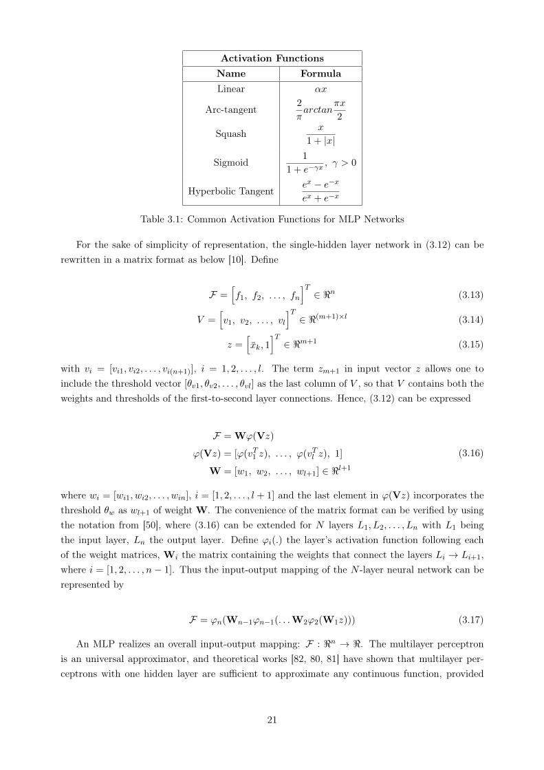
Activation FunctionsName FormulaLinear ↵x

Arc-tangent2

⇡

arctan

⇡x

2

Squashx

1 + |x|

Sigmoid1

1 + e

��x, � > 0

Hyperbolic Tangente

x � e

�x

e

x+ e

�x

Table 3.1: Common Activation Functions for MLP Networks

For the sake of simplicity of representation, the single-hidden layer network in (3.12) can berewritten in a matrix format as below [10]. Define

F =

h

f1, f2, . . . , fn

iT2 <n (3.13)

V =

h

v1, v2, . . . , vl

iT2 <(m+1)⇥l (3.14)

z =

h

xk, 1

iT2 <m+1 (3.15)

with vi = [vi1, vi2, . . . , vi(n+1)], i = 1, 2, . . . , l. The term zm+1 in input vector z allows one toinclude the threshold vector [✓v1, ✓v2, . . . , ✓vl] as the last column of V , so that V contains both theweights and thresholds of the first-to-second layer connections. Hence, (3.12) can be expressed

F = W'(Vz)

'(Vz) = ['(v

T1 z), . . . , '(v

Tl z), 1]

W = [w1, w2, . . . , wl+1] 2 <l+1

(3.16)

where wi = [wi1, wi2, . . . , win], i = [1, 2, . . . , l + 1] and the last element in '(Vz) incorporates thethreshold ✓w as wl+1 of weight W. The convenience of the matrix format can be verified by usingthe notation from [50], where (3.16) can be extended for N layers L1, L2, . . . , Ln with L1 beingthe input layer, Ln the output layer. Define 'i(.) the layer’s activation function following eachof the weight matrices, Wi the matrix containing the weights that connect the layers Li ! Li+1,where i = [1, 2, . . . , n� 1]. Thus the input-output mapping of the N -layer neural network can berepresented by

F = 'n(Wn�1'n�1(. . .W2'2(W1z))) (3.17)

An MLP realizes an overall input-output mapping: F : <n ! <. The multilayer perceptronis an universal approximator, and theoretical works [82, 80, 81] have shown that multilayer per-ceptrons with one hidden layer are sufficient to approximate any continuous function, provided

21

that there are enough hidden nodes. In nonlinear system identification problems, the number ofthe output nodes is equal to the number of the system outputs, and the number of the networkinput is equal to the dimension of system inputs. From (3.17) network input-output mappingF : <n ! < is clearly highly nonlinear in Wi, and training an multilayer perceptron is analogueto estimating this parameter vector. After the learning process is complete, the network mappingcan be assigned as a model of the system for control and other engineering applications.

Although modern research has revealed considerable drawbacks of the multilayer perceptronwith respect to many applications, it is still the most widely known and used neural networkarchitecture, sometimes even being used as a synonym for NN. One of the advantages is thatthe architecture permits possible extensions in the use of more than one hidden layer. Multiplehidden layers make the network much more powerful and complex, recently giving rise to the deeplearning approach [95, 96, 97]. Additionally, accuracy is usually very high, given the nonlinearlyparametrized structure, it often results in better approximation performance than the equivalentlinearly parametrized network approaches. Also, due to the optimization of the hidden layerweights the multilayer perceptron can be extremely powerful and usually requires fewer neuronsand parameters than other model topologies to perform a comparable approximation accuracy.Further, this property can be characterized as a high information compression capability.

3.3.2 High Order Neural Network

Since artificial neural networks for nonlinear system identification is that they categorize as"black-box" models, one of the drawbacks is that information about the system’s structure andparameters may not be intuitive for interpretation. Higher Order Neural Networks (HONNs) helpalleviate this problem by including nodes at the input layer that contribute the network witha better understanding of the input behavior and their dynamics. Essentially, the inputs aretransformed via higher-order functions such as squares, cubes, or sines in which the net inputto a neuron node is a weighted sum of products of its inputs. Although, this approach has beenshown to accelerate training in some applications, in practice, only second order networks are used.The major drawback of HONNs is that the required number of weights to accommodate all thehigh-order correlations increases exponentially with the dimensionality of the input vector [67, 98].

The authors in [67, 99, 100] showed that HONNs have great computational, storage and learningcapabilities. The order or structure of a HONN can be adapted according to the order or structureof a given problem, this advantage provide a more specialized and efficient approach in solvingthese problems. Additionally, a priori knowledge about the system can also be incorporated in aHONN when it is available. Also, results in [101] demonstrated HONNs to be at least as powerful asany other feedforward neural topology of same order. Another research [102], by using a piecewiselinear HONN with the structure consisting of two layers of modifiable weights, has shown HONNto be seven times faster than standard feedforward neural networks when simulating the XORproblem. Another comparison with FNNs is that [103] points out HONNs to significantly decreasethe needed training time for a given task. The authors in [67] studied the approximation andlearning properties of a class of recurrent HONNs and successfully applied these topologies to the

22

identification of dynamical systems. The structure of HONNs can be expressed as

xi = �aixi(t) + bi

LX

k=1

wikz(Ik) (3.18)

z(Ik) =Y

j2Ik

d

mj(k)j (x, u) (3.19)

d =

2

6

6

6

6

6

6

6

6

6

6

6

6

6

6

6

4

S(x1)S(x2)

...S(xn)S(u1)S(u2)

...S(un)

3

7

7

7

7

7

7

7

7

7

7

7

7

7

7

7

5

(3.20)

where u 2 <m, x 2 <n, I1, I2, . . . , IL is a collection of L nonordered subsets of 1, 2, . . . , L, L �m + n is the number of high order interactions, mj(k) are nonnegative integers, ai and bi arepositive constants and are fixed during training, wik are the adjustable net weights and mj(k)

are nonnegative integers. The dynamic behavior of the overall network is described by expressing(3.18) in vector notation as

x = Ax+BW

Tz (3.21)

where x = [x1 . . . xn]T , W = [wi . . . wn] 2 <L⇥n, A := diag(�a1,�a2, . . . ,�an) is an n⇥n diagonal

matrix, also a stability matrix and B := diag(�b1,�b2, . . . ,�bn) is an L⇥ L diagonal matrix.

It is proved in the literature [67, 94] that HONNs satisfy the conditions of the Stone-WeierstrassTheorem, guaranteeing to approximate any continuous function over a compact set. According to[98], high-order neural networks of any order can be trained by applying any of the learningalgorithms proposed for first-order neural networks.

3.3.3 Radial Basis Function Neural Networks

Radial Basis Function (RBF) neural networks are three-layer models with an input layer, ahidden layer and output layer where a linear combination of the hidden inputs neurons occurs.Each of the hidden nodes performs a nonlinear transformation of the input, by means of RadialBasis Functions. For the RBF network, the basis function at the i -th hidden neuron is given by

fi(x) = �(kx � cik) (3.22)

23

where k.k denotes a norm that is typically assumed to be Euclidean, x 2 <n the input vector, ciwith i = 1, . . . , n is the unit centre in the input space and �(.) a nonlinear activation function.The basis functions are radially symmetric with the centre on ci in the input space, hence theyare named radial basis functions. The overall input-output response of an n-input m-output RBFnetwork is a mapping fRBF : <n ! <m. Mathematically,

fRBFi =

nHX

j=1

✓j,i�j =

nHX

j=1

✓j,i�(kx � cik;�j), 1 i nO (3.23)

where ✓j,i are the weights of the linear combiners, �j are some positive scalars called the widths,ci are the RBF centers and nH is the number of hidden nodes. Also, (3.23) can be rewritten invector form as

fRBF (x) = W� (3.24)

where

W =

2

6

6

6

6

4

w11 w12 · · · w1n

w21 w22 · · · w2n...

... . . . ...wn1 wn2 · · · wnn

3

7

7

7

7

5

and � =

2

6

6

6

6

4

�(kx � c1k)�(kx � c2k)

...�(kx � cnk)

3

7

7

7

7

5

(3.25)

The RBF network is known to be a general function approximator, and theoretical research haveconcluded that the choice of �(.) is not essential for network approximation capabilities [104, 105].Nonetheless, deciding the nonlinearity of the hidden nodes according to the application can oftenimprove performance. Examples of common activation functions for local and global RBFs areshown in table 3.2, where r = kx � cik, � is a real number usually called receptive width or thewidth of the locally-tuned function which describes the declivity of the hyperbolic cone used in theradial function.

Figure 3.3 shows the architecture of a RBF network. The topology of the RBF network issimilar to that of the single-hidden layer perceptron, and the difference lies in the description ofthe hidden node. Hence, its input to the hidden layer connection transforms the input into adistance from a point in the input space, unlike in the multilayer perceptron (MLP), where it istransformed into a distance from a hyperplane in the input space. Then, while the hidden neuronsof a MLP with sigmoidal activation covers wide regions in the input space, the hidden neuronsof a RBF covers small specific regions. Thus, multilayer networks are more efficient as functionapproximators. Now, for tasks such as pattern classification, RBF networks tends to outperformthe MLP [106].

24

Activation FunctionsName Formula

Gaussian exp

✓

r

2

�

2

◆

Inverse Multiquadric�

r

2+ �

2�� 1

2

Linear r

Cubic r

3

Shifted Logarithms ln

�

r

2+ �

2�

Thin Plate Splines r

2ln(r)

Pseudo Potential Functions (1� exp

✓

� r

2

�

2

◆

ln(r))

Table 3.2: Common Activation Functions for RBF Networks

Inputlayer

Hiddenlayer

Outputlayer

...

...

...

x1

x2

xn�1

xn

�(.)

�(.)

�(.)

�(.)

�(.)

�(.)

�(.)

�(.)

�(.)

�(.)

�(.)

�(.)

w1

⌃

wj

wn

fRBF (x)

Figure 3.3: Radial Basis Function Neural Network

In general, the RBF network has a nonlinear-in-the-parameters structure. However, learningcan be implemented in two steps. First, a learning mechanism is performed to select a suitableset of RBF centers and widths. This effectively determines the hidden layer of the RBF network.After this step, learning the remaining output-layer weights becomes a linear problem. In thisaspect, the RBF network becomes a linear-in-the-parameters structure. This is true only after thehidden layer has been fixed separately before the second step. Because of this property, learningprocedures for the RBF network can be straightforward and reliable [5].

25

3.3.4 Fuzzy Neural Networks

Fuzzy neural networks have their origin from fuzzy sets and fuzzy inference systems, which wereinitially introduced by [107] as a extension of Boolean logic. A basic configuration of a n-input m-output fuzzy system is shown in 3.4. A fuzzy system consists of four basic components: a fuzzifier,a fuzzy rule set, a fuzzy inference engine, and a defuzzifier. The fuzzifier deals with a mappingfrom the input space to the fuzzy sets defined in the input space. The fuzzy rule base consists of aset of nF linguistic rules in the forms of IF-THEN values. The fuzzy inference engine is a decision-making logic that uses the fuzzy rules provided by the fuzzy rule base to determine a mapping fromthe fuzzy sets in the input space to the fuzzy sets in the output space. The efficiency of a fuzzyinference engine heavily relies on the knowledge base of the problem considered. The defuzzifierprovides a mapping from the fuzzy sets in <m to the crisp outputs y 2 <n. A class of fuzzysystems typically used in practice is constructed based on product inference, singleton fuzzificationand centroid or weighted average defuzzification [5]. Such fuzzy systems can be represented asseries expansions of fuzzy basis functions known as fuzzy basis function (FBF) networks or models[108, 43].

A ni-input m-output fuzzy system can be mathematically expressed as m single-output fuzzysubsystems [5]. The rule base of the ith fuzzy subsystem consists of nF rules defined as follows:

RB

ij : IF x1 is A1,j AND ... AND xnI is AnI,j , THEN yi is Bi

j (3.26)

where 1 j nF for 1 l n are the inputs to the fuzzy system; yiis the ith output of the fuzzysystem, 1 i m; and Ai,j and B

ij are the fuzzy sets described by fuzzy membership functions

µAl,j(xl) and µBi

j(yi), respectively. Under the assumptions of singleton fuzzifier, product inference,

and centroid defuzzifier, the input-output mapping of such a fuzzy system, fFBF : <n ! <mcanbe demonstrated to have the following form [108, 43, 109]

fFBFi(x) =

PnFj=1 y

ij(Qn

l=1 µAl,j(xl))

PnFj=1(

Qnl=1 µAl,j

(xl)), 1 i m (3.27)

where y

ij is the point at which µBi

j(yi) achieves its maximum value. Define

�i(x) =Qn

l=1 µAl,j(xl)

PnFj=1(

Qnl=1 µAl,j

(xl)), 1 i nF (3.28)

which are referred to as fuzzy basis functions (FBFs). Then the fuzzy system (3.27) is equal to anFBF expansion,

fFBFi(x) =nFX

j=1

�j(x)✓j,i, 1 i m (3.29)

where ✓j,i are coefficients of parameters of the FBF model.

26

Inference

Rule Base

Fuzzifier DefuzzifierCrispx

Crispy

Figure 3.4: Fuzzy System Architecture, adapted from [5]

Fuzzy systems are universal approximators, and theoretical studies have proved that the FBFnetwork (3.29) can approximate any continuous functions to within any degree of accuracy, pro-vided that a sufficient number of fuzzy rules are used [108, 43, 109]. Although the FBF network isderived within the framework of fuzzy logic, it obviously has many similarities to neural networkssuch as the RBF network. In fact, under some conditions, singleton neuro-fuzzy systems are equiv-alent to normalized RBF networks [110, 111]. An advantage of the FBF network is that linguisticinformation from human knowledge in the form of the fuzzy IF-THEN rules can be integrated intothe model, allowing improved understanding of the process and exploitation of prior knowledge[112].

Generally fuzzy systems are employed in engineering applications where the number of inputsand outputs is small. This is because the number of rules or FBFs grows exponentially as thenumber of inputs and outputs increases. This curse of "rule explosion" limits further uses offuzzy systems to complex large systems. Furthermore, several restrictions and constraints mustbe assumed on the fuzzy in order to keep it interpretable. Several applications of fuzzy systems inareas such as financial prediction, nonlinear systems identification and control has been proposed[113, 114, 115]. Notice that the FBF network (3.29) has a linear-in-the-parameters structure oncethe rules have been specified.

3.3.5 Wavelet Neural Networks

Wavelet neural networks (WNNs) were introduced in the 1990s [44, 45], based on wavelettransform theory initiated by the works in [116]. Wavelet transform theory was developed toanalyse signals with varied frequency resolutions such as a unifying idea of looking at non stationarysignals at various time locations. For reviews and tutorials on wavelets see, for example [117, 118].There are some significant differences between wavelet series expansions and classical Fourier series,which are

• Wavelets are local in both the frequency domain (via dilations) and in the time domain (viatranslations). On the other hand, Fourier basis functions are localised only in the frequencydomain but not in the time domain. Small frequency changes in the Fourier transform will

27

cause changes everywhere in the time domain.

• Many classes of functions can be described in a more compact way by wavelets than by theFourier series. Also, the wavelet basis functions are more effective than classical Fourier basisones in achieving a comparable function approximation.

The above advantages give wavelets strong compression abilities via dilation and translationproperties, helping alleviate the local minima problem of the classical sigmoidal neural networks[44]. The wavelets refer to a family of functions generated from one single function '(.) by theoperation of dilation and translation. In the continuous case it takes the following form

i(x) =| a�1/2i | '(x� bi

ai) (3.30)

where x = [x1, . . . , xn] 2 <n is the input vector and the parameters ai, bi 2 < and i 2 Z are namedthe scale and translation parameters, respectively. The parameter ai is a scaling or dilation factorand bi a translation factor of the original function '(.).

In the standard form of a wavelet neural network, output is given by

f(x) =

mX

i=1

wi i(x) =

mX

i=1

wi | ai |�1/2'(

x� bi

ai) (3.31)

where m is the number of hidden neurons, i is the wavelet activation function of i-th unit ofthe hidden layer and wi is the weight connecting the i-th unit of the hidden layer to the output-layer unit. An example of the WNN architecture is shown in 3.5.It should be noted that for then-dimensional input space, the multivariate wavelet-basis function can be computed by the tensorproduct of n single wavelet-basis functions given by

'(x) =

nY

j=1

'(xj) (3.32)

Wavelet neural networks have the universal approximation property [119, 44]. Some examples ofwavelet families used as activation function are shown in table 3.3, where r = x

Tx and k = dim(x),

whereas there are many other types of wavelet functions which depend on the specific application.It should be noted in (3.31) that the wavelet neural networks have a linearly parametrized structure.However, if the translation and dilation parameters ai and bi are handled as adjustable parametersthe referred network becomes nonlinearly parametrized and can be trained like any multilayerperceptron neural network [120].

Wavelet theory and networks have been widely employed in applications in diverse fields, suchas system identification [46, 121] geophysics [122], signal denoising [123], electric load forecasting[124], time-series prediction [125] and control [126]. However, according to [120], wavelet networkssuffer from "curse of dimensionality". To train a wavelet neural network, the gradients with respectto all the unknown parameters must be expressed explicitly. Thus, the calculation of gradients may

28

Inputlayer

Hiddenlayer

Outputlayer

...

...

...

x1

x2

xn�1

xn

(.)

(.)

(.)

(.)

(.)

(.)

(.)

(.)

(.)

(.)

(.)

(.)

w1

⌃

wj

wn

f(x)

Figure 3.5: Wavelet Neural Network

Activation FunctionsName Formula

Gaussian derivative (k � r)e

�r/2

Mexican Hat2p3⇡

1/4(k � r

2)e

�r2/2

Morlet Wavelet cos(5r)e

�r2/2

Haar wavelet

8

>

<

>

:

1 if 0 x < 1/2

� 1 if 1/2 x < 1

0 otherwise

Table 3.3: Common Activation Functions for Wavelet Networks

be heavy and difficult in high-dimensional models as the number of candidate wavelet terms oftenincreases with the model order. Also, another problem is how to determine the initial number ofwavelets associated with the network. These major drawbacks often limit the application of WNNsto low dimensions for dynamical identification problems.

3.4 Categories of Learning Algorithms

Neural networks are trained by two main types of learning algorithms: supervised and unsu-pervised learning algorithms. In addition, there is a third type, reinforcement learning, which canbe regarded as a special form of supervised learning [4]. They can be classified as shown in Fig.3.6:

29

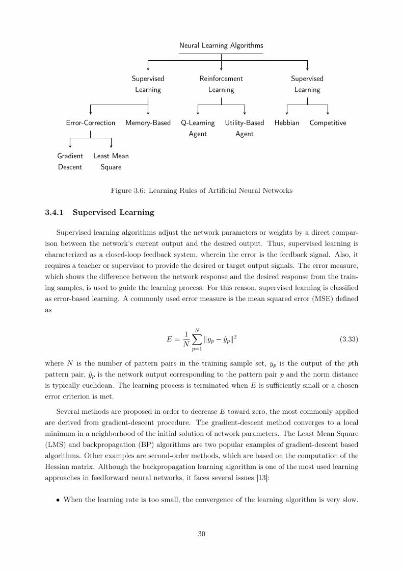
Neural Learning Algorithms

SupervisedLearning

Error-Correction

GradientDescent

Least MeanSquare

Memory-Based

ReinforcementLearning

Q-LearningAgent

Utility-BasedAgent

SupervisedLearning

Hebbian Competitive

Figure 3.6: Learning Rules of Artificial Neural Networks

3.4.1 Supervised Learning

Supervised learning algorithms adjust the network parameters or weights by a direct compar-ison between the network’s current output and the desired output. Thus, supervised learning ischaracterized as a closed-loop feedback system, wherein the error is the feedback signal. Also, itrequires a teacher or supervisor to provide the desired or target output signals. The error measure,which shows the difference between the network response and the desired response from the train-ing samples, is used to guide the learning process. For this reason, supervised learning is classifiedas error-based learning. A commonly used error measure is the mean squared error (MSE) definedas

E =

1

N

NX

p=1

kyp � ypk2 (3.33)

where N is the number of pattern pairs in the training sample set, yp is the output of the pthpattern pair, yp is the network output corresponding to the pattern pair p and the norm distanceis typically euclidean. The learning process is terminated when E is sufficiently small or a chosenerror criterion is met.

Several methods are proposed in order to decrease E toward zero, the most commonly appliedare derived from gradient-descent procedure. The gradient-descent method converges to a localminimum in a neighborhood of the initial solution of network parameters. The Least Mean Square(LMS) and backpropagation (BP) algorithms are two popular examples of gradient-descent basedalgorithms. Other examples are second-order methods, which are based on the computation of theHessian matrix. Although the backpropagation learning algorithm is one of the most used learningapproaches in feedforward neural networks, it faces several issues [13]:

• When the learning rate is too small, the convergence of the learning algorithm is very slow.

30

However, if it is too large, the algorithm becomes unstable and diverges.

• Another challenge is the presence of local minima in the error surface that affects the perfor-mance of the backpropagation algorithm [4]. This may result in an undesirable performanceif the learning algorithm is trapped at a local minima located far from a global minima.

• Neural network are prone to overtraining and obtain worse generalization performance whenusing backpropagation methods. Thus, validation and suitable stopping criteria are necessaryin the cost function minimization procedures.

• Gradient-based learning may require long training times. For example, the mean square errormay remain high in a number of interactions and suddenly reach small values. Thus, withoutprior experience, it may be difficult to estimate the training time given a particular task.

The extreme learning machine (ELM) has been proposed in order to alleviate the aforemen-tioned drawbacks for single-hidden layer neural networks. The advantages of this learning algo-rithm is being easy to implement, tends to reach the smallest training error, obtains the small-est norm of weights and the reasonable generalization performance and also runs extremely fast[13, 127, 128, 73].

3.4.2 Unsupervised Learning

Unsupervised learning refers to algorithms that seeks to learn structure in the absence of eitheran identified output or feedback. They do not require the desired outputs to be known. Duringtraining, only input patterns are presented to the neural network which automatically adaptsthe weights to its connections to cluster the input patterns intro groups with similar features.Thus, unsupervised learning is purely based on the correlations among the input data, and isused to find the significant patterns or features in the input data without the help of a teacher.Making it particularly suitable for biological learning in that it does not rely on a teacher and ituses intuitive primitives like neural competition and cooperation. For this reason, unsupervisedlearning is classified as output-based learning.

A criterion is needed to terminate the learning process. Without a stopping criterion, a learningprocess continues even when a pattern, which does not belong to the training patterns set, ispresented to the network. The network is adapted according to a constantly changing environment.Examples of unsupervised learning algorithms include Hebbian learning, competitive learning,Adaptive Resonance Theory and the self-organizing maps (SOM). In general, unsupervised learningis slow to settle under stable conditions [4].

3.4.3 Reinforcement Learning

Reinforcement learning describes a class of computational algorithms that specifies how anartificial agent can learn to select actions in order to maximize the received reward over time.Instead of using a teacher to give target outputs, reinforcement learning is a learning procedure

31

that rewards the neural network for its good output result and punishes it for the bad outputresult [4].

As mentioned before, reinforcement learning is a special case of supervised learning, wherethe exact desired output is unknown. Unlike in supervised learning problems, in reinforcement-learning problems, there are no labeled examples of correct and incorrect behavior. However, unlikeunsupervised learning problems, a reward signal can be perceived. Since the teacher supplies onlyfeedback about success or failure of an answer. In some applications, it may be more plausiblethan supervised learning since a fully specified correct answer might not always be available to thelearner or even the teacher. It is based only on the information as to whether or not the actualoutput is close to the estimate. Furthermore, explicit computation of derivatives is not required.However, this results in a slower learning process. In control applications, if the controller of asystem still works accurately after an input, the output is labeled good; otherwise, it is judgedbad. The evaluation of the binary output, also called external reinforcement, is used as the errorsignal. Examples of reinforcement learning algorithms are Temporal Difference (TD) learning,Monte-Carlo methods, Q � learning, genetic and evolutionary algorithms [129].

3.4.4 Offline and Online Identification

The previous learning methods can be applied in a online or offline fashion for system iden-tification. For the offline case, the measured data is first stored and then the model parametersare estimated. On the other hand, the online identification is performed parallel to the experi-ment and the algorithm estimates the parameters of the model when new data is available duringthe operation of the model. It should be noted that for nonlinear systems, the system operationcan vary with time or the real system input space may be different from the one which was usedfor offline identification. In order to achieve good identification results, both the structure andthe weights of the neural network model may need to be modified in response to changes in theplant characteristics. Thus, the main advantage of online identification is that parameter valuesusing online estimation can vary with time, but parameters estimated using offline methods donot. Hence, adaptive control is an example of such an application where it is useful to identify themodel online, simultaneously with the acquisition of measurements [130].

32

Chapter 4

Online Neuro-Identification of NonlinearSystems using Extreme LearningMachine

4.1 Motivation and Difference Between Neural Networks and Ex-treme Learning Machines

In the last decade, the extreme learning machine (ELM) approach has been proposed fortraining unified single hidden layer feedforward neural networks (SLFNs). In ELM, the hiddennodes are randomly initiated and remain fixed during the learning process without iterativelytuning. Moreover, the hidden nodes in ELM are not even necessary to be identical to a neuron.The only free parameters which need to be tuned are the weights between the hidden layer andthe output layer. Hence, ELM is classified as a linearly parameterized model which reduces tosolving a linear system. Compared to conventional feedforward neural network learning techniques,ELM is considerably efficient and turns to reach a global optimum. Theoretical studies haveproved that despite the presence of randomly generated hidden nodes, ELM preserves the universalapproximation capability of SLFNs [13, 71, 127].

ELM models share the same architecture of a traditional feedforward neural network, howeverthere are some subtle differences that make the ELM models remarkably attractive compared toANNs. In a conventional ANN model, both the input and the output layers parameters are spec-ified in the training process. Thus, a nonlinear technique is typically required, which may havelimitations such as slow iterative training and local minima trapping. ELM alleviates these limi-tations by eliminating the need for tuning the hidden layer parameters from the training process.As the input layer parameters are randomly generated according to a probability distribution, thetraining involves determining the output layer weights only. Since training involves a linear leastsquares problem, the achieved solution by the ELM approach is extremely fast and is a globaloptimum [13, 71, 127].

33

In spite of the aforementioned advantages, as the number of hidden neurons increase, an over-parametrized ELM suffers from ill conditioning problem when learning laws based on recursiveleast squares are performed [131]. This drawback may lead to an unbounded growth of the modelparameters and unbounded model predictions, specially when the system is under external distur-bances or unknown dynamics. For any general case, the convergence of ELM based identifier isnever guaranteed to be stable. Hence it is of extreme importance to guarantee the convergence sta-bility and approximation error boundedness for control related applications. To tackle this issue,stable online learning algorithms based on Lyapunov stability theory are developed in this chap-ter. The Lyapunov approach provides a stability guarantee and performs well with no undesirableparameter growth.

This chapter is organized as follows. Sections 4.2-4.3 provides a mathematical description ofthe ELM along with the problem formulation. In section 4.4, the identification model and the stateestimate error equation is introduced followed by the stable adaptive laws for adjusting the outputweights together with a Lyapunov analysis in section 4.5. Section 4.6 shows several simulationresults. Finally, section 4.7 presents the summary from this chapter.

4.2 Description of Extreme Learning Machine

The output of a unified single hidden-layer feedforward neural network (SLFN) with ˜

N hiddennodes can be represented by

fN (x) =

NX

i=1

�i�(x;wi, ✓i) (4.1)

where wi 2 <n is the weight vector connecting the input layer to the ith hidden node, �i is theoutput weight connecting the ith hidden node to the output node, ✓i is the bias of the ith hiddennode with respect to the input x 2 <n, �(x;wi, ✓i) is the output of the ith hidden node with respectto the input x and �(.) is the activation function of ELM. Commonly used activation functions�(.) include sigmoid and hyperbolic tangent functions.

The standard SLFN with ˜

N hidden nodes with activation function �(.) can approximate N

arbitrary distinct samples (xk, yk) 2 <n ⇥ <m with zero error, it then implies that there exist �i,wi and ✓i such that

X

�i�(xk;wi, ✓i) = yk, k = 1, . . . , N (4.2)

The above equation can be written compactly as

H� = Y (4.3)

where

34

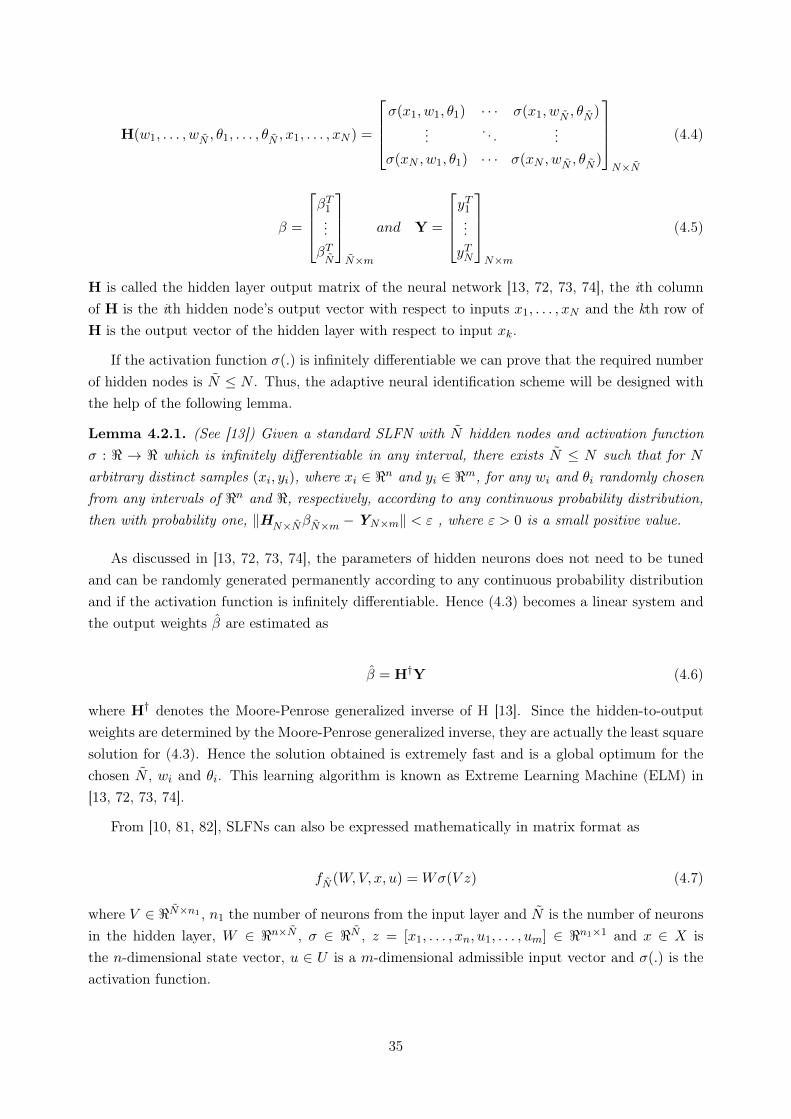
H(w1, . . . , wN , ✓1, . . . , ✓N , x1, . . . , xN ) =

2

6

6

4

�(x1, w1, ✓1) · · · �(x1, wN , ✓N )

... . . . ...�(xN , w1, ✓1) · · · �(xN , wN , ✓N )

3

7

7

5

N⇥N

(4.4)

� =

2

6

6

4

�

T1...�

TN

3

7

7

5

N⇥m

and Y =

2

6

6

4

y

T1...y

TN

3

7

7

5

N⇥m

(4.5)

H is called the hidden layer output matrix of the neural network [13, 72, 73, 74], the ith columnof H is the ith hidden node’s output vector with respect to inputs x1, . . . , xN and the kth row ofH is the output vector of the hidden layer with respect to input xk.

If the activation function �(.) is infinitely differentiable we can prove that the required numberof hidden nodes is ˜

N N . Thus, the adaptive neural identification scheme will be designed withthe help of the following lemma.

Lemma 4.2.1. (See [13]) Given a standard SLFN with ˜

N hidden nodes and activation function� : < ! < which is infinitely differentiable in any interval, there exists ˜

N N such that for N

arbitrary distinct samples (xi, yi), where xi 2 <n and yi 2 <m, for any wi and ✓i randomly chosenfrom any intervals of <n and <, respectively, according to any continuous probability distribution,then with probability one, kHN⇥N�N⇥m �YN⇥mk < " , where " > 0 is a small positive value.

As discussed in [13, 72, 73, 74], the parameters of hidden neurons does not need to be tunedand can be randomly generated permanently according to any continuous probability distributionand if the activation function is infinitely differentiable. Hence (4.3) becomes a linear system andthe output weights ˆ

� are estimated as

ˆ

� = H†Y (4.6)

where H† denotes the Moore-Penrose generalized inverse of H [13]. Since the hidden-to-outputweights are determined by the Moore-Penrose generalized inverse, they are actually the least squaresolution for (4.3). Hence the solution obtained is extremely fast and is a global optimum for thechosen ˜

N , wi and ✓i. This learning algorithm is known as Extreme Learning Machine (ELM) in[13, 72, 73, 74].

From [10, 81, 82], SLFNs can also be expressed mathematically in matrix format as

fN (W,V, x, u) = W�(V z) (4.7)

where V 2 <N⇥n1 , n1 the number of neurons from the input layer and ˜

N is the number of neuronsin the hidden layer, W 2 <n⇥N , � 2 <N , z = [x1, . . . , xn, u1, . . . , um] 2 <n1⇥1 and x 2 X isthe n-dimensional state vector, u 2 U is a m-dimensional admissible input vector and �(.) is theactivation function.

35

Remark 1. The mathematical description for unified SLFN present in (4.1) is quite common inELM literature. However, for ease of use in stability analysis and without loss of generality, theSLFN matrix representation (4.7) will be adopted for the remaining of this chapter.

4.3 Problem Formulation

Consider the following nonlinear differential equation

x = F (x, u, v, t), x(0) = x0 (4.8)

where x 2 X is the n-dimensional state vector, u 2 U is a m-dimensional admissible input vector,v 2 V ⇢ <q is a vector of time varying uncertain variables and F : X ⇥ U ⇥ V ⇥ [0,1) 7! <n is acontinuous map. In order to have a well-posed problem, we assume that X,U, V are compact setsand F is locally Lipschitzian with respect to x in X⇥U ⇥V ⇥ [0,1), such that (4.8) has a uniquesolution.

We assume that the following can be established:

Assumption 1. On a region X ⇥ U ⇥ V ⇥ [0,1)

kd(x, u, v, t)k d0 (4.9)

where

d(x, u, v, t) = F (x, u, v, t)� f(x, u) (4.10)

f is an unknown map, d are internal or external disturbances, and ¯

d0 , such that ¯

d0 > d0 � 0, is aknown constant. Note that (4.9) is verified when x and u evolve on compact sets and the temporaldisturbances are bounded.

Hence, except for the Assumption 1, we say that F (x, u, v, t) is an unknown map and our aim isto design an online SLFN identifier with random hidden nodes and adaptive output weights whichare determined by the ELM and Lyapunov synthesis for (4.8) to ensure the state error convergence,which will be accomplished despite the presence of approximation error and disturbances.

4.4 Identification Model and State Estimate Error Equation

We start by presenting the identification model and the definition of the relevant errors asso-ciated with the problem.

Now, by adding Ax to and subtracting from (4.8), where A 2 <n⇥n is an arbitrary Hurwitzmatrix, then the system becomes

36

x = Ax+ g(x, u) + d(x, u, v, t) (4.11)

where g(x, u) = f(x, u)�Ax describes the system nonlinearity.

From Lemma 1 and by using SLFNs, the nonlinear mapping g(x, u) can be replaced byW

⇤�(VRz) plus an approximation error term "(x, u). More exactly, (4.11) becomes

x = Ax+BW

⇤�(VRz) +B"(x, u) + d(x, u, v, t) (4.12)

where B 2 <n⇥n is a scaling matrix, VR 2 <N⇥n1 is a randomly generated matrix according to anygiven continuous probability distribution and W

⇤ 2 <n⇥N is the “optimal” or ideal matrix whichcan be defined as

W

⇤:= argmin

(W )

⇢

sup

z2⌦z

|W�(VRz)� g(z)|�

(4.13)

where ⌦z is a predefined compact set for z, which is defined as

⌦z = {z 2 <n1: kxk Mz} (4.14)

where Mz is a positive constant specified by the designer. The approximation, reconstruction, ormodeling error "(x, u) in (4.12) is a quantity that arises due to the incapacity of SLFN to matchthe unknown map g(x, u). In general, W

⇤ is unknown and needs to be estimated in functionapproximation. Let ˆ

W be the estimate of W ⇤, respectively, and the weight estimation error be˜

W =

ˆ

W �W

⇤. From Lemma 1, the following can be established

Assumption 2. On a compact set ⌦z, the ideal neural network weight and the NN approximationerror are bounded by

kW ⇤kF wm, k"(x, u)k "0 (4.15)

where wm and "0 are known positive constants.

Remark 2. Assumption 1 is usual in identification or robust control literature. Assumption 2 isquite natural since g is continuous and their arguments evolve on compact sets.

Remark 3. It should be noted that W

⇤ was defined as being the value of ˆ

W that minimizes theL1-norm difference between g(x, u) and ˆ

W�(VRz). The scaling matrix B from (4.12) is introducedto manipulate the magnitude of uncertainties and hence the magnitude of the approximation error.This procedure improves the performance of the identification process.

Remark 4. It is noteworthy that in the original ELM algorithm the output weight W is ad-justed based on the least-square error method. However in the proposed identification scheme,the adaptive law for updating the output weight ˆ

W is derived using Lyapunov methods in order

37

to guarantee the stability of the entire identification process. Nonetheless, as in the original ELMalgorithm, the hidden node parameters are also randomly determined.

Remark 5. Notice that the proposed neuro-identification scheme is a black-box methodology,hence the external disturbances and approximation error are related. Based on the system inputand state measurements, the uncertain system (including the disturbances) is parameterized bya neural network model plus an approximation error term. However, the aim for presenting theuncertain system in the form (4.12), where the disturbance d is explicitly considered, is also tohighlight that the proposed scheme is in addition valid in the presence of unexpected boundedchanges in the system dynamics that can emerge, for instance, due to environment change, agingof equipment or faults.

The structure (4.12) suggests an identification model of the form

˙

x = Ax+B

ˆ

W�(VRz)� l (4.16)

where x is the estimated state, B 2 <n⇥n is a positive diagonal matrix introduced to adjust themagnitude of uncertainties and hence the magnitude of the approximation error, and l is a vectorfunction to be defined afterwards. It will be demonstrated that the identification model (4.16)used in conjunction with a convenient adjustment law for ˆ

W , to be proposed in the next section,ensures the convergence of the state error to a neighborhood of the origin, even in the presence ofthe approximation error and disturbances, whose radius depends on the design parameters.

By defining the state estimation error as x := x�x, from (4.12) and (4.16), we obtain the stateestimation error equation

˙

x := Ax+B

˜

W�(VRz) + ⇤� l (4.17)

where ˜

W =

ˆ

W �W

⇤ is the estimated parameter error for the output weight and ⇤ = �B"(x, u)�d(x, u, v, t) is a bounded residual term.

Remark 6. The sections 4.2-4.3 are motivated by [20]. However, in contrast to [20], it is consid-ered in the model for identification a feedback function l with a time variant gain to ensure theconvergence of the state errors to zero.

4.5 Adaptive Laws and Stability Analysis

We now state and prove the main theorem of this chapter.

Theorem 4.5.1. Consider the class of general nonlinear systems described by (4.8) which satisfiesAssumptions 1-2, the identification model (4.16) with

l =

�0x

�min(K)[kxk+ �1exp(��2t)](4.18)

38

Let the weight adaptation law be given by

˙

ˆ

W = ��wh

kxk( ˆW �W0) +BKx�(VRz)

i

(4.19)

�w > 0, W0 is a constant matrix, VR are the randomly generated hidden layer weights and K is amatrix such that

K = P + P

T (4.20)

where P is a positive definite matrix. Then, the signal errors x and ˜

W are bounded. In addition,if �0 > ↵0 where ↵0 is a positive constant, then limt!1x(t) = 0.

Proof. Consider the Lyapunov function candidate

¯

V = x

TPx+

k ˜

Wk2F2�w

(4.21)

By evaluating the time derivative of (4.21) along the trajectories of (4.17) and (4.19), we obtain

˙

¯

V =

˙

x

TPx+ x

TP

˙

x+

tr

⇣

˜

W

T ˙

˜

W

⌘

�w

=

⇣

x

TA

T+ �

T˜

W

TB

T � ⇤

T⌘

Px� x

TKl

+ x

TP

⇣

Ax+B

˜

W � � ⇤

⌘

+

tr

⇣

˜

W

T ˙

˜

W

⌘

�w

(4.22)

where ˙

˜

W =

˙

ˆ

W , since ˙

W

⇤= 0.

By using (4.20) and the Lyapunov equation A

TP + PA = �Q, the Lyapunov derivative can

be written as

˙

¯

V =� x

TQx+ x

TKB

˜

W � � x

TK⇤� x

TKl

� tr

n

˜

W

Th

kxk⇣

ˆ

W �W0

⌘

+BKx�

Tio (4.23)

Furthermore, by using the following representations

tr

n

˜

W

TBKx�

To

= x

TKB

˜

W � (4.24)

and further rearranging terms, (4.23) implies

˙

¯

V = �x

TQx� x

TK⇤� x

TKl � tr

n

˜

W

Th

kxk⇣

ˆ

W �W0

⌘io

(4.25)

By considering the facts

39

2tr

h

˜

W

T⇣

ˆ

W �W0

⌘i

= k ˜

Wk2F +

�

�

�

⇣

ˆ

W �W0

⌘

�

�

�

2

F� k(W ⇤ �W0)k2F

k⇤(t)k ⇤0

(4.26)

where ⇤0 > 0, (4.26) results

˙

¯

V � �min(Q) kxk2 � 0.5

�

�

�

˜

W

�

�

�

2

Fkxk

� [(�0 � ↵0) kxk � �1↵0exp(��2t)]kxk+ �1exp(��2t)

kxk(4.27)

where �min(Q) denotes the minimum eigenvalue of Q and ↵0 = ⇤0 kKkF + 0.5 kW ⇤ �W0k2F .

At first, note that (4.27) implies

˙

¯

V ��min(Q) kxk2 � 0.5

�

�

�

˜

W

�

�

�

2

Fkxk+ ↵0 kxk (4.28)

or, by completing the square,

˙

¯

V = ��min(Q)

✓

kxk � ↵0

2�min(Q)

◆2

� 0.5

�

�

�

˜

W

�

�

�

2

Fkxk+ ↵

20

4�min(Q)

(4.29)

Hence, ˙

¯

V < 0 outside the compact set ⌦0 =

n⇣

x,

˜

W

⌘

| kxk ↵x or

�

�

�

˜

W

�

�

�

F ↵W

o

where

↵x = ↵0/�min(Q) and ↵W = (↵0/2�min(Q))

1/2. Thus, since ↵x and ↵W are positive constants,by employing usual Lyapunov arguments [62], we concluded that all error signals are uniformlybounded.

Define now

⌦ =

n⇣

x,

˜

W

⌘

| kx(t)k ⌘exp(��2t), ⌘ = �1↵0/(�0 � ↵0)

o

(4.30)

Note that the numerator in the bracket of (4.27) is greater than zero for kxk > ⌘exp(��2t) (orx 2 ⌦

c), hence

˙

¯

V ��min(Q) kxk2 (4.31)

Further, since ¯

V is bounded from below and non-increasing with time, we have

limt!1

Z t

0kx(⌧)k2 d⌧

¯

V (0)� ¯

V1�min(Q)

< 1 (4.32)

where limt!1 ¯

V (t) =

¯

V1 < 1. Notice that, based on (4.17), with the bounds on x, ˜

W and l, ˙

x isalso bounded. Thus, ˙

¯

V is uniformly continuous. Hence, by applying the Barbalat’s Lemma [62],we conclude that limt!1x(t) = 0 for all x 2 ⌦

c.

40

Once the synchronization error x(t) has entered ⌦, it will remain in ⌦ forever, due to (4.30)and (4.31). Consequently, we conclude that limt!1x(t) = 0 holds in the large, i.e., whatever theinitial value of

⇣

x(t),

˜

W (t)

⌘

(inside or outside ⌦).

Remark 7. It should be noted that resizing unknown nonlinearities has a positive impact on theidentification performance. The matrix B is introduced to attenuate the effect of uncertainties, ascan be seen in (4.29).

4.6 Simulation

This section presents four examples to validate the theoretical results and to show effectivenessin the presence of disturbances. The examples were chosen based on their bounded and complexnature, with promising applications in engineering. In all simulations, Solver ode23 (Bogacki-Shampine) of Matlab/Simulinkr, with a relative tolerance of 1e-6 was used to obtain the numericalsolutions. Also, the time in which the exponential function in (4.18) is turned off was set to ts = 3s

for all cases. First, the identification of a Chen system under disturbances using the proposedmethodology is achieved, after it is considered a hyperchaotic finance system submitted to thepresence of disturbances. An example of complex hyperchaotic system with 7 states is identifiedto show the feasibility of the ELM model for higher dimensional systems. Finally, a proposedalgorithm in the literature [1] is used here for comparison.

4.6.1 Chen System

Consider the unified chaotic system [132], which is described by

x = (25↵+ 10)(y � x) + dx

y = (28� 35↵)x� xz + (29↵� 1)y + dy

z = xy �✓

8 + ↵

3

◆

z + dz

(4.33)

where x, y and z are state variables and is always chaotic in the whole interval ↵ 2 [0, 1] and dx, dyand dz are unknown disturbances. It should be also noted that system (4.33) becomes the Lorenzsystem for ↵ = 0, Chen system for ↵ = 1. In particular, system (4.33) bridges the gap between theLorenz system and the Chen system. In the following simulation, we consider the Chen system.

To identify the chaotic system (4.33), the proposed identification model (4.16) and the adaptivelaw (4.19) were implemented. It should be noted that VR is randomly assigned and remains fixedthrough the simulation. The design parameters were chosen as �w = 0.001, �0 = 0.1, �1 = 1,�2 = 0.00001, the sigmoid function is �(.) = 100/1 + exp� 1(.), the design matrices are

A =

2

6

4

�10.5 0 0

0 �9 0

0 0 �9.5

3

7

5

, B = 10

2 ⇥

2

6

4

4.1 0 0

0 3.9 0

0 0 4

3

7

5

(4.34)

41

with W0 = 0 and P = 0.5⇥ I3⇥3, where I is the identity matrix. The chosen inputs are

z =

h

x y z x

2y

2z

21

i

(4.35)

The chosen initial conditions for the system are x(0) = �1.5, y(0) = �2, z(0) = �5, x(0) = 5,y(0) = 5, z(0) = 5 and ˆ

W = 0. To check the robustness of the proposed method, it is consideredthe presence of the following time-dependent disturbance

d(x, u, v, t) =

2

6

4

3sin(7t)k(x, y, z)k10cos(9t)x

cos(20t) + 10exp(�t)

3

7

5

(4.36)

for the system (4.33). We consider the emergence, at t = 5s, of disturbances of the form (4.36).

The performances in the estimation of state variable are shown in Fig. 4.1-4.3. It can be seenthat the simulations confirm the theoretical results, that is, the algorithm is stable and the residualstate error is small. The Frobenius norms associated to the estimated weight matrix W is shown inFig. 4.4. After a transient phase, due to the large initial uncertainty, this norm seems to converge,indicating that most of the state estimation error has been removed. It should be noted that thetransient can be shaped according to the user’s desired convergence.

Figure 4.1: Performance in the estimation of x

In the simulations of the proposed algorithm, the design matrices A, B, P and K were initiallychosen as identity matrices. In the sequence, these values were adjusted, by a trial and errorprocedure, to fulfill requirements of performance (such as small residual state error and transient).As a remark, the design parameters can be appropriately chosen so as to suit the requirementson overshoot and settling time of the parameter estimation. It was selected appropriate gains for

42

the design parameters to force a fast tracking; however, the transient can be adjusted arbitrarilydepending on the project requirements. This gives additional flexibility and control on the proposedmodel’s performance.

Figure 4.2: Performance in the estimation of y

Figure 4.3: Performance in the estimation of z

43

Figure 4.4: Frobenius norm of the estimated weight matrix W

From Fig. 4.4, it can be concluded that the identification scheme is robust in the presence of dis-turbances and unknown dynamics, handling abrupt perturbations with practically no degradationof performance.

4.6.2 Hyperchaotic Finance System

Consider a hyperchaotic finance system described by [133]

x = z + (y � a)x+ u+ dx

y = 1� by � x

2+ dy

z = �x� cz + dz

u = �dxy � ku� du

(4.37)

where a, b, c, d and k are constant parameters and dx, dy, dz and du are unknown disturbances.It was considered that a = 0.9, b = 0.2, c = 1.2, d = 0.2 and k = 0.17. Notice that system (4.37)satisfies assumption 1, since the state variables evolve on compact sets.

To identify the uncertain system (4.37), the proposed identification model (4.16) and the adap-tive law (4.19) were implemented. The design parameters were chosen as �w = 0.01, �0 = 0.1,�1 = 1, �2 = 0.00001, the sigmoid function is �(.) = 150/1 + exp � 1(.), the matrices parametersare

44

A =

2

6

6

6

6

4

�29 0 0 0

0 �30.5 0 0

0 0 �30 0

0 0 0 �28

3

7

7

7

7

5

, B = 10

2 ⇥

2

6

6

6

6

4

1.1 0 0 0

0 0.8 0 0

0 0 1.2 0

0 0 0 1

3

7

7

7

7

5

(4.38)

with W0 = 0 and P = 0.05⇥ I4⇥4, where I is the identity matrix. The chosen inputs are

z =

h

x y z x

2y

2z

21

i

(4.39)

The chosen initial conditions for the system are x(0) = 1, y(0) = 2.5, z(0) = 0.5, u(0) = 0.5,x(0) = �2, y(0) = �2, z(0) = �2, u(0) = �2 and ˆ

W = 0. To check the robustness of the proposedmethod, it is considered the presence of the following time-dependent disturbance

d(x, u, v, t) =

2

6

6

6

6

4

8sin(7t)u

10cos(9t)x

2

(cos(20t) + 5exp(�t))y

2sin(20t) + 3cos(15t)

3

7

7

7

7

5

(4.40)

We consider the emergence, at t = 5s, of disturbances of the form (4.40).

The performances in the estimation of state variable are shown in Fig. 4.5-4.8. It can be seenthat the simulations confirm the theoretical results, that is, the algorithm is stable and the residualstate error is small. The Frobenius norms associated to the estimated weight matrix W is shownin Fig. 4.9. One can find that the system outputs achieved by the proposed neural controller stillasymptotically track the desired trajectories well.

Figure 4.5: Performance in the estimation of x

45

Figure 4.6: Performance in the estimation of y

Figure 4.7: Performance in the estimation of z

46

Figure 4.8: Performance in the estimation of u

Figure 4.9: Frobenius norm of the estimated weight matrix W

47

4.6.3 Hyperchaotic System

Consider a hyperchaotic system described by [134]

x1 = ↵(x3 � x1) + dx1

x2 = ↵(x4 � x2) + dx2

x3 = �x1 � x1x5 � x3 + x6 + dx3

x4 = �x2 � x2x5 � x4 + x7 + dx4

x5 = x1x3 + x2x4 � �x5 + dx5

x6 = k1x1 + k2x3 + dx6

x7 = k1x2 + k2x4 + dx7

(4.41)

where ↵, �, �, k1 and k2 are constant parameters and dx1, dx2, dx3, dx4, dx5, dx6 and dx7 areunknown disturbances. It was considered that ↵ = 14, � = 3, � = 50, k1 = �5 and k2 = �4.Notice that system (4.41) satisfies assumption 1, since the state variables evolve on compact sets.

To identify the uncertain system (4.41), the proposed identification model (4.16) and the adap-tive law (4.19) were implemented. The design parameters were chosen as �w = 0.1, �0 = 0.1,�1 = 1, �2 = 0.00001, the sigmoid function is �(.) = 150/1+ exp� 0.1(.), the matrices parametersare

A = �16⇥

2

6

6

6

6

6

6

6

6

6

6

6

4

1.1 0 0 0 0 0 0

0 0.9 0 0 0 0 0

0 0 1.2 0 0 0 0

0 0 0 1.3 0 0 0

0 0 0 0 1 0 0

0 0 0 0 0 0.8 0

0 0 0 0 0 0 1

3

7

7

7

7

7

7

7

7

7

7

7

5

, B = 50⇥

2

6

6

6

6

6

6

6

6

6

6

6

4

1 0 0 0 0 0 0

0 0.9 0 0 0 0 0

0 0 1.2 0 0 0 0

0 0 0 1 0 0 0

0 0 0 0 1 0 0

0 0 0 0 0 1.1 0

0 0 0 0 0 0 0.8

3

7

7

7

7

7

7

7

7

7

7

7

5

(4.42)

with W0 = 0 and P = 0.05⇥ I7⇥7, where I is the identity matrix. The chosen inputs are

z =

h

x1 x2 x3 x4 x5 x6 x7 1

i

(4.43)

The chosen initial conditions for the system are x1(0) = 0, x2(0) = 1, x3(0) = 2, x4(0) = 3,x5(0) = 4, x6(0) = 5, x7(0) = 6, x1(0) = �20, x2(0) = �30, x3(0) = �40, x4(0) = 20, x5(0) = 40,x6(0) = 50, x7(0) = 40 and ˆ

W = 0. To check the robustness of the proposed method, it isconsidered the presence of the following time-dependent disturbance

48

d(x, u, v, t) = 2 kxk

2

6

6

6

6

6

6

6

6

6

6

6

4

sin(t)u

1.2sin(2t)

cos(4t)

1.2sin(t)

1.1sin(2t)

0.5sin(4t)

exp(�0.5t)

3

7

7

7

7

7

7

7

7

7

7

7

5

(4.44)

where x = [x1 x3 x3 x4 x5 x6 x7]T . We consider the emergence, at t = 5s, of disturbances of the

form (4.44).

The performances in the estimation of state variable are shown in Fig. 4.10-4.16. It can beseen that the simulations confirm the theoretical results, that is, the algorithm is stable and theresidual state error is small. The Frobenius norms associated to the estimated weight matrix W

is shown in Fig. 4.17. One can find that the system outputs achieved by the proposed neuralcontroller still asymptotically track the desired trajectories well.

Figure 4.10: Performance in the estimation of x1

49

Figure 4.11: Performance in the estimation of x2

Figure 4.12: Performance in the estimation of x3

50

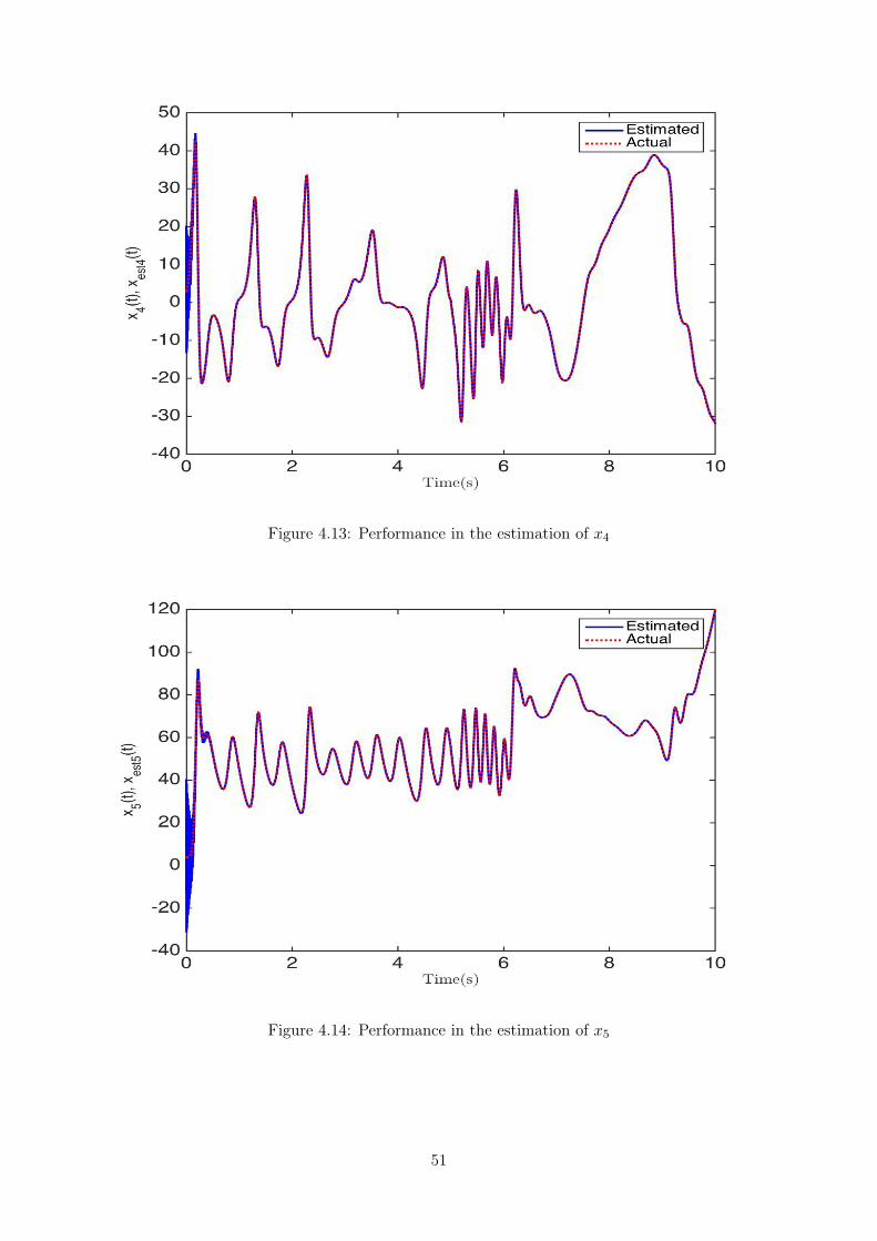
Figure 4.13: Performance in the estimation of x4

Figure 4.14: Performance in the estimation of x5

51

Figure 4.15: Performance in the estimation of x6

Figure 4.16: Performance in the estimation of x7

52

Figure 4.17: Frobenius norm of the estimated weight matrix W

4.6.4 Comparison with Ref. [1]

To illustrate the advantages of the proposed methodology, the identification model introducedin [1] is used here for comparison. Consider the Lyapunov based ELM algorithm proposed in [1]described as

˙

z = Az(t) +

ˆ

W

T�

˙

ˆ

W = ��eT(4.45)

where the state vector z 2 <n⇥1, � is the activation function for the regressor vector VRz and VR

the hidden layer weight matrix with random values. The Lorenz system is considered, where ↵ = 0

in (4.33). The sigmoid function is �(.) = 150/1 + exp � 0.001(.). The design matrix A is chosenas [1], where

A =

2

6

4

�60 0 0

0 �60 0

0 0 �120

3

7

5

(4.46)

The chosen initial conditions for the system are x(0) = 1, y(0) = 2.5, z(0) = 0.5, x(0) = 5,y(0) = 5, z(0) = 5 and ˆ

W = 0. It was stated in [1] that were chosen 12 inputs, as it was notspecified, they are chosen here as

53

z = [x y z x

2y

2z

2xy xz yz xyz x

2y x

2z] (4.47)

The initial conditions and design parameters of the proposed algorithm of this chapter forthis simulation are the same as in 4.6.1. To check the robustness of the proposed method, it isconsidered the presence of the following time-dependent disturbance for the comparison

d(x, u, v, t) = kwk

2

6

4

3sin(7t)u

10cos(9t)

(cos(20t) + 10exp(�t))y

3

7

5

(4.48)

where w = [x y z]

T . We consider the emergence, at t = 5s, of disturbances of the form (4.40).

Figs. 4.18-4.20 show the state error norms comparisons for each state variable. It should bepointed out that the adjustment of the design parameters in [1] was not trivial given the parameterdrift, mainly due to the lack of tuning parameters in the learning law ˆ

W for compensating thisdrawback. Furthermore, it seems that the absence of a robustifying term for the adaptive parameterlaw in [1] has a negative impact on the performance when the system is under external disturbance,as can be seen in Figs. 4.18-4.22

Figure 4.18: Performance comparison in the estimation of x

54

Figure 4.19: Performance comparison in the estimation of y

Figure 4.20: Performance comparison in the estimation of z

55

Figure 4.21: Frobenius norm of the estimated weight matrix W

Figure 4.22: Frobenius norm of the estimated weight matrix W

56

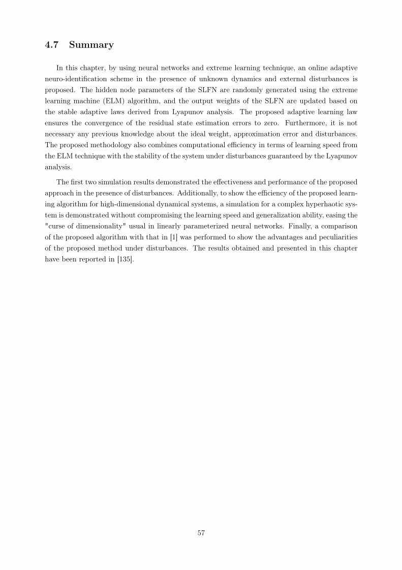
4.7 Summary

In this chapter, by using neural networks and extreme learning technique, an online adaptiveneuro-identification scheme in the presence of unknown dynamics and external disturbances isproposed. The hidden node parameters of the SLFN are randomly generated using the extremelearning machine (ELM) algorithm, and the output weights of the SLFN are updated based onthe stable adaptive laws derived from Lyapunov analysis. The proposed adaptive learning lawensures the convergence of the residual state estimation errors to zero. Furthermore, it is notnecessary any previous knowledge about the ideal weight, approximation error and disturbances.The proposed methodology also combines computational efficiency in terms of learning speed fromthe ELM technique with the stability of the system under disturbances guaranteed by the Lyapunovanalysis.

The first two simulation results demonstrated the effectiveness and performance of the proposedapproach in the presence of disturbances. Additionally, to show the efficiency of the proposed learn-ing algorithm for high-dimensional dynamical systems, a simulation for a complex hyperhaotic sys-tem is demonstrated without compromising the learning speed and generalization ability, easing the"curse of dimensionality" usual in linearly parameterized neural networks. Finally, a comparisonof the proposed algorithm with that in [1] was performed to show the advantages and peculiaritiesof the proposed method under disturbances. The results obtained and presented in this chapterhave been reported in [135].

57

Chapter 5

Identification of Unknown NonlinearSystems based on Multilayer NeuralNetworks

5.1 Motivation

Feedforward multilayer neural networks are of particular interest in this Master’s thesis, sinceit has been shown that with enough hidden units and under certain conditions they are capableof approximating any nonlinear mapping [80, 81, 86]. Moreover, linearly parametrized neuralnetworks typically suffers the so-called "curse of dimensionality", where as the input dimension ofthe system increases the number of nodes demanded to approximate nonlinear mappings increasesexponentially. Thus, the computational demands, both in memory and computational time, canbe significantly high for multiple-input multiple-output systems.

Also, nonlinearly parametrized neural networks provide greater approximation power thanlinearly parametrized models. For instance, the author in [136, pp. 11] shows that for certainclasses of functions, single-hidden layer neural network models with a sigmoid activation functioncan achieve a given approximation accuracy with a number of nodes that is linearly dependenton the dimension of the input vector. Thus, the above properties make SHLNNs well worth forinvestigating its application for system identification of nonlinear systems.

This chapter is organized as follows. Sections 5.2-5.3 give a brief review of the SHLNNs alongwith the problem formulation. In section 5.4, the design procedure of the adaptive neural iden-tifier and the state estimate error equation is introduced followed by the stable adaptive laws foradjusting the output weights based on a Lyapunov synthesis approach in section 5.5. Section 5.6shows the simulation results. Finally, section 5.8 presents the summary from this chapter.

58

5.2 Single Hidden Layer Neural Networks

A class of multilayer NNs used here can be expressed mathematically in matrix form as

gnn(W,V, x, u) = W�(V z) (5.1)

where V 2 <n2⇥(n1+1), n1 is the number of neurons from the input layer, n2 is the numberof neurons in the hidden layer, W 2 <n⇥n2 , � 2 <n2 is a basis function vector and z =

[x1, . . . , xn, u1, . . . , um, 1] 2 <n1+1, where n1 = n + m. In standard SHLNNs each entry of �(.)is a linear combination of either an external input or the state passed through a scalar activationfunction s(.). Commonly used s(.) are the sigmoid and hyperbolic tangent function [10].

Universal approximation results in [10, 67] indicate that:

Property 1. Let s(.) be a nonconstant, bounded and monotone increasing continuous function.Let ⌦z be a compact subset of <n and g(z) be a real valued continuous function on ⌦z. Then forany arbitrary µ > 0, there exists an integer n2 and ideal matrices W

⇤ and V

⇤ such that

max

z2⌦z

|g(z)� gnn(W⇤, V

⇤, z)| < µ (5.2)

Based on Property 1, we have

g(z) = W

⇤�(V

⇤z) + "(z) (5.3)

with "(z) satisfying maxz2⌦z |"(z)| < µ, 8z 2 ⌦z.

5.3 Problem Formulation

Consider the following nonlinear differential equation

x = F (x, u, v, t), x(0) = x0 (5.4)

where x 2 X is the n-dimensional state vector, u 2 U is a m-dimensional admissible input vector,v 2 V ⇢ <q is a vector of time varying uncertain variables and F : X ⇥ U ⇥ V ⇥ [0,1) 7! <n is acontinuous map. In order to have a well-posed problem, we assume that X,U, V are compact setsand F is locally Lipschitzian with respect to x in X⇥U ⇥V ⇥ [0,1), such that (5.4) has a uniquesolution.

We assume that the following can be established:

Assumption 1. On a region X ⇥ U ⇥ V ⇥ [0,1)

59

kd(x, u, v, t)k d0 (5.5)

where

d(x, u, v, t) = F (x, u, v, t)� f(x, u) (5.6)

f is an unknown map, d are internal or external disturbances, and ¯

d0 , such that ¯

d0 > d0 � 0, is aknown constant. Note that (5.5) is verified when x and u evolve on compact sets and the temporaldisturbances are bounded.

Hence, except for the Assumption 1, we say that F (x, u, v, t) is an unknown map and our aimis to design a NNs-based identifier for (5.4) to ensure the state error convergence, which will beaccomplished despite the presence of approximation error and disturbances.

5.4 Identification Model and State Estimate Error Equation

We start by presenting the identification model and the definition of the relevant errors asso-ciated to the problem.

By adding and subtracting Ax, where A 2 <n⇥n is an Hurwitz matrix, (5.4) can be rewrittenas

x = Ax+ g(x, u) + d(x, u, v, t) (5.7)

where g(x, u) = f(x, u)�Ax.

By using SHLNNs, the nonlinear mapping g(z) can be replaced by W

⇤�(V

⇤z) plus an approx-

imation error term "(x, u). More exactly, (5.4) becomes

x = Ax+BW

⇤�(V

⇤z) +B"(x, u) + d(x, u, v, t) (5.8)

where B 2 <n⇥n is a scaling matrix, W ⇤ 2 <n⇥n2 and v

⇤ 2 <n2⇥(n1+1) are the “optimal” or idealmatrices, which can be defined as

(W

⇤, V

⇤) := argmin

(W,V )

⇢

sup

z2⌦z

|W�(V z)� g(z)|�

(5.9)

Let ˆ

W and ˆ

V be the estimates of W ⇤ and V

⇤, respectively, and the weight estimation errorsbe ˜

W =

ˆ

W �W

⇤ and ˜

V =

ˆ

V � V

⇤. From (5.3), the following can be established

Assumption 2. On a compact set ⌦z, the ideal neural network weight and the NN approximationerror are bounded by

60

kW ⇤kF wm, kV ⇤kF vm, k"(x, u)k "0 (5.10)

where wm, vm and "0 are known positive constants.

Remark 1. Assumption 1 is usual in identification. Assumption 2 is quite natural since g iscontinuous and their arguments evolve on compact sets.

Remark 2. It should be noted that W

⇤ and V

⇤ were defined as being the values of ˆ

W and ˆ

V

that minimize the L1-norm difference between g(x, u) and ˆ

W�(

ˆ

V z). The scaling matrix B from(5.8) is introduced to manipulate the magnitude of uncertainties and hence the magnitude of theapproximation error. This procedure improves the performance of the identification process.

Remark 3. As multilayer neural networks are classified as nonlinear in the parameters approx-imators, since the hidden layer weight V appears in a nonlinear fashion, it is far more complexto derive the learning algorithms in comparison with the linear in the parameters models. Whenapplying function approximators such as ˆ

W�

⇣

ˆ

V z

⌘

for solving the identification problem, it is

desired to have a linearly parameterized form in terms of ˜

W and ˜

V . One approach [10] is byapplying the Taylor series expansion of �(V ⇤

z) about ˆ

V z, where we have

�(V

⇤z) = �(

ˆ

V z)� ˆ

�

0˜

V z +⇥ (5.11)

where �0 = @�(V ⇤z)@V ⇤z

�

�

�

V zand ⇥ represents the high order terms in the Taylor expansion.

The structure (5.8) suggests an identification model of the form

˙

x = Ax+B

ˆ

W�(

ˆ

V z)� l0x� l (5.12)

where l0 > 0, l is a vector function to be defined afterwards, x is the estimated state and x := x�x

is the state estimation error. It will be demonstrated that the identification model (5.12) used inconjunction with convenient adjustment laws for ˆ

W and ˆ

V to be proposed in the next section,ensures the convergence of the state error to a neighborhood of the origin, even in the presence ofthe approximation error and disturbances, whose radius depends on some design parameters.

From (5.8) and (5.12), we obtain the state estimation error equation

˙

x = Ax+B

ˆ

W�(

ˆ

V z)�BW

⇤�(V

⇤z)�B"(x, u)� d(x, u, v, t)� l0x� l (5.13)

From (4.11), we can rewrite the state estimation error equation as

˙

x = Ax+B

˜

W�(

ˆ

V z) +B

ˆ

W �

0˜

V z �B

˜

W �

0(

ˆ

V z)

˜

V z � ⇤� l0x� l (5.14)

where ⇤ = �BW

⇤⇥�B"(x, u)� d(x, u, v, t) is a bounded residual term.

61

5.5 Adaptive Laws and Stability Analysis

We now state and prove the main theorem of this chapter.

Theorem 5.5.1. Consider the class of general nonlinear systems described by (5.4), which satisfiesAssumptions 1-2, the identification model (5.12) with

l =

�0x

�min(K)[kxk+ �1exp(��2t)](5.15)

Let the weights adaptation laws be given by

˙

ˆ

W = ��W

2↵W kxk⇣

ˆ

W �W0

⌘

+BKx�

T �BKx

⇣

�

0ˆ

V z

⌘T�

(5.16)

˙

ˆ

V = ��Vh

2↵V kxk⇣

ˆ

V � V0

⌘

+ �

0ˆ

W

TBKxz

Ti

(5.17)

where �0 � 0, �1 > 0, �2 > 0, �W > 0, �V > 0, ↵W > 0, ↵V > 0, W0 and V0 are constantmatrices, K is a matrix such that

K = P + P

T (5.18)

and P is a positive definite matrix. Then, if �0 = 0, the estimation errors ˜

W and ˜

V are bounded,and x is uniformly ultimately bounded with ultimate bound ↵x. If �0 > ↵3, where ↵3 > 0, the stateerror converges to zero, i.e., limt!1x(t) = 0.

Proof. Consider the Lyapunov function candidate

¯

V = x

TPx+

�

�

�

˜

W

�

�

�

2

F

2�W+

�

�

�

˜

V

�

�

�

2

F

2�V(5.19)

By evaluating the time derivative of (5.19) along the trajectories of (5.14), (5.16) and (5.17),we obtain

˙

¯

V =� x

TQx+ x

TKB

˜

W � � x

TKB

˜

W �

0˜

V z + x

TKB

ˆ

W �

0˜

V z � x

TK⇤

� tr

⇢

˜

W

T

2↵W kxk⇣

ˆ

W �W0

⌘

+BKx�

T �BKx

⇣

�

0ˆ

V z

⌘T��

� tr

n

˜

V

Th

2↵V kxk⇣

ˆ

V � V0

⌘

+ �

0ˆ

W

TBKxz

Tio

� l0x2 � x

TKl

(5.20)

where A

TP + PA = �Q, Q is a Hurwitz matrix, ˙

˜

W =

˙

ˆ

W and ˙

˜

V =

˙

ˆ

V , since ˙

W

⇤= 0 and ˙

V

⇤= 0.

Furthermore, by using the following representations

62

tr

n

˜

W

TBKx�

To

= x

TKB

˜

W �

tr

⇢

˜

W

TBKx

⇣

�

0ˆ

V z

⌘T�

= x

TKB

˜

W �

0ˆ

V z

tr

n

˜

V �

0ˆ

W

TBKxz

To

= x

TKB

ˆ

W �

0˜

V z

(5.21)

and further rearranging terms, (5.20) results

˙

¯

V =� x

TQx� x

TK⇤� tr

n

˜

W

Th

2↵W kxk⇣

ˆ

W �W0

⌘io

� tr

n

˜

V

Th

2↵V kxk⇣

ˆ

V � V0

⌘io

� l0x2 � x

TKl

(5.22)

By considering the facts

� ˜

V +

ˆ

V = V

⇤,

2tr

h

˜

W

T⇣

ˆ

W �W0

⌘i

=

�

�

�

˜

W

�

�

�

2

F+

�

�

�

⇣

ˆ

W �W0

⌘

�

�

�

2

F� k(W ⇤ �W0)k2F

2tr

h

˜

V

T⇣

ˆ

V � V0

⌘i

=

�

�

�

˜

V

�

�

�

2

F+

�

�

�

⇣

ˆ

V � V0

⌘

�

�

�

2

F� k(V ⇤ � V0)k2F

�

�

�

0(t)

�

� �0d, k⇤(t)k ⇤0, kz(t)k z0, 8t � 0

(5.23)

where �0d, ⇤0 and z0 are positive constants, and, in the sequence, by completing the square, (5.22)implies

˙

¯

V = �kxk"

l0 kxk+ ↵W

✓

�

�

�

˜

W

�

�

�

F� ↵1

2↵W

◆2

+ ↵W

�

�

�

˜

V

�

�

�

2

F� ↵0

#

(5.24)

where ↵0 = ↵

21/4↵w + ↵2 + ↵w kW ⇤ �W0k2F + ↵W kV ⇤ � V0k2F , ↵1 = z0↵0d kKBkF kW ⇤kF and

↵2 = ⇤0 kKkF .

Hence, with ˙

¯

V < 0 outside the compact set ⌦ =

n⇣

x,

˜

W,

˜

V

⌘

�

� kxk ↵x or

�

�

�

˜

WF

�

�

�

↵W or�

�

�

˜

V

�

�

�

F ↵V

o

where ↵x = ↵0/l0, ↵W = (↵0/l0)1/2

+ ↵1/2↵W and ↵V = (↵0/↵V )1/2. Thus, since

↵x, ↵W and ↵V are positive constants, by employing usual Lyapunov arguments [11], we concludedthat all error signals are uniformly bounded. In addition, since l0, ↵W and ↵V can be arbitrarilyselected, x(t) is uniformly ultimately bounded with ultimate bound ↵x.

In case that �0 > ↵3, (5.22) implies

˙

¯

V � [�min(Q) + l0] kxk2 �↵3�1 [kxk � ⌘exp(�2t)]

⌘x+ �1exp(�2t)(5.25)

where ↵3 = ↵1 + ↵2 + ↵W kW ⇤ �W0k2F + ↵V kV ⇤ � V0k2F and ⌘ = �1↵3/(�0 � ↵3).

Define now

⌦ =

n⇣

x,

˜

W

⌘

�

� kx(t)k ⌘exp(��2t)o

(5.26)

63

Note that the numerator in the bracket of (5.25) is greater than zero for kxk > exp(��2t) (orx 2 ⌦

c), hence

˙

¯

V � [�min(Q) + l0] kxk2 (5.27)

Further, since ¯

V is bounded from below and non increasing with time, we have

limt!1

Z t

0kx(⌧)k2 d⌧

¯

V (0)� ¯

V1�min(Q) + l0

< 1 (5.28)

where limt!1 ¯

V (t) =

¯

V1 < 1. Notice that, based on (5.14), with the bounds on x, ˜

W , ˜

V , andl, ˙

x is also bounded. Thus, ˙

¯

V is uniformly continuous. Hence, by applying the Barbalat’s Lemma[62], we conclude that limt!1x(t) = 0 for all x 2 ⌦

c.

Once the synchronization error x(t) has entered ⌦, it will remain in ⌦ forever, due to (5.26).Consequently, we conclude that limt!1x(t) = 0 holds in the large, i.e., whatever the initial valueof⇣

x(t),

˜

W (t),

˜

V (t)

⌘

(inside or outside ⌦).

Corollary 5.5.2. Consider the class of general nonlinear systems described by (5.4), with satisfiesAssumptions 1-2, the identification model (4.12), (5.15-5.17) with �2 = 0. Then, the state errorx(t) converges to the residual set

⌅ =

�

x

�

� kx(t)k �1↵1

(5.29)

where ↵t = exp(��2ts) and ts is the time in which the exponential function in (5.15) is turned off.

Remark 4. Corollary 5.5.2 establish an interesting peculiarity of the proposed method. Theexponential function used in the identification model can be turned off when the residual stateerror has entered to any desired neighborhood of the origin. It is important to overcome numericalerrors that can appear when the exponential function on the right-hand side of (5.15) has practicallydecayed to zero.

Remark 5. It should be noted that the disturbances in an infinite horizon are related to theresidual state error. However, this residual error can be controlled, for instance, by the designparameter l0 and matrix B. For further details, see [66].

5.6 Simulation

This section presents four examples to validate the theoretical results. In the following simula-tions, it should be noted that the identification models does not depend explicitly on perturbations.Moreover, in all simulations, Solver ode23 (Bogacki-Shampine) of Matlab/Simulinkr, with a rel-ative tolerance of 1e-6 was used to obtain the numerical solutions. Also, the time in which the

64

exponential function in (5.15) is turned off was set to ts = 3s for all cases. First, the identifica-tion of a Chen system using the proposed methodology is achieved. Then, the same system andidentification model are submitted to the presence of disturbances. To check the performance forhigher dimensional systems, a complex hyperchaotic system with 7 states is identified. Finally, aproposed algorithm in the literature [2] is used here for comparison.

5.6.1 Chen System with proposed algorithm

Consider the unified chaotic system [132], which is described by

x = (25↵+ 10)(y � x)

y = (28� 35↵)x� xz + (29↵� 1)y

z = xy �✓

8 + ↵

3

◆

z

(5.30)

where x, y and z are state variables and is always chaotic in the whole interval ↵ 2 [0, 1]. It shouldbe also noted that system (5.30) becomes the Lorenz system for ↵ = 0, Chen system for ↵ = 1. Inparticular, system (5.30) bridges the gap between the Lorenz system and the Chen system. In thefollowing simulation, we consider the Chen system.

To identify the chaotic system (5.30), the proposed identification model (5.12) and the adaptivelaws (5.14) and (5.16) were implemented. The design parameters were chosen as ↵W = 1, ↵V = 1

�W = 0.02, �V = 0.001, ↵W = 0.5, ↵V = 0.5, l0 = 10, the sigmoid function is �(.) = 100/1+exp�1(.), the design matrices are

A =

2

6

4

�7.8 0 0

0 �7.8 0

0 0 �7.8

3

7

5

, B =

2

6

4

121 0 0

0 127.6 0

0 0 143

3

7

5

(5.31)

with W0 = 0, V0 = 0 and P = 0.05⇥ I3⇥3, where I is the identity matrix. The chosen inputs are

z =

h

x y z x

2y

2z

21

i

(5.32)

The chosen initial conditions for the system and the identification model are x(0) = 2, y(0) = 1,z(0) = 2, x(0) = 5, y(0) = 5, z(0) = 5, ˆ

W (0) = 0 and ˆ

V (0) = 0. The performances in theestimation of state variables are shown in Fig. 5.1-5.3. It can be seen that the simulations confirmthe theoretical results, that is, the algorithm is stable and the residual state error is small. TheFrobenius norms associated to the estimated weight matrices W and V are shown in Fig. 5.4 and5.5, respectively. After a transient phase, due to the large initial uncertainty, these norms seem toconverge, indicating that most of the state estimation error has been removed. It should be notedthat the transient can be shaped according to the user’s desired convergence.

In the simulations of the proposed algorithm, the design matrices A, B, P and K were initiallychosen as identity matrices. In the sequence, these values were adjusted, by a trial and error

65

procedure to fulfill requirements of performance.

Figure 5.1: Performance in the estimation of x

Figure 5.2: Performance in the estimation of y

66

Figure 5.3: Performance in the estimation of z

Figure 5.4: Frobenius norm of the estimated weight matrix W

67

Figure 5.5: Frobenius norm of the estimated weight matrix V

Figure 5.6: Performance in the estimation of x

To check the robustness of the proposed method, it is now considered an additional case with

68

the presence of the following time-dependent disturbance:

d(x, u, v, t) = 3sin(t) kxk+ 50sin(200t) + 10cos(400t)⇥

2

6

4

0

1

1

3

7

5

(5.33)

where x = [x y z]

T . Note that the disturbance appears only to states y and z in (5.30). Keepingall design parameters and initial conditions as before, we consider the emergence, at t = 5s, ofdisturbances of the form 5.33. The obtained results are shown in Fig. 5.6-5.8. From Fig. 5.9 and5.10, it can be concluded that the identification scheme is robust in the presence of perturbationwithout, practically, any degradation of performance.

Figure 5.7: Performance in the estimation of y

Figure 5.8: Performance in the estimation of z

69

Figure 5.9: Frobenius norm of the estimated weight matrix W

Figure 5.10: Frobenius norm of the estimated weight matrix V

70

5.6.2 Hyperchaotic System

Consider a hyperchaotic system described by [134]

x1 = ↵(x3 � x1) + dx1

x2 = ↵(x4 � x2) + dx2

x3 = �x1 � x1x5 � x3 + x6 + dx3

x4 = �x2 � x2x5 � x4 + x7 + dx4

x5 = x1x3 + x2x4 � �x5 + dx5

x6 = k1x1 + k2x3 + dx6

x7 = k1x2 + k2x4 + dx7

(5.34)

where ↵, �, �, k1 and k2 are constant parameters and dx1, dx2, dx3, dx4, dx5, dx6 and dx7 areunknown disturbances. It was considered that ↵ = 14, � = 3, � = 50, k1 = �5 and k2 = �4.Notice that system (5.34) satisfies assumption 1, since the state variables evolve on compact sets.

To identify the uncertain system (5.34), the proposed identification model (5.12) and the adap-tive laws (5.14) and (5.16) were implemented. The design parameters were chosen as �V = 1,�w = 0.01, ↵W = 1, ↵V = 1, l0 = 10, the sigmoid function is �(.) = 150/1 + exp � 1(.), thematrices parameters are

A = �20⇥ I7⇥7, B = 100⇥ I7⇥7, P = 0.05⇥ I7⇥7 (5.35)

where I is the identity matrix, with W0 = 0, V0 = 0. The chosen inputs are

z =

h

x1 x2 x3 x4 x5 x6 x7 1

iT(5.36)

The chosen initial conditions for the system are x1(0) = 0, x2(0) = 1, x3(0) = 2, x4(0) = 3,x5(0) = 4, x6(0) = 5, x7(0) = 6, x1(0) = �50, x2(0) = �40, x3(0) = �30, x4(0) = 20, x5(0) = 40,x6(0) = 50, x7(0) = 400, ˆ

W (0) = 0 and ˆ

V (0) = 0. To check the robustness of the proposedmethod, it is considered the presence of the following time-dependent disturbance

d(x, u, v, t) = 1.8kxk

2

6

6

6

6

6

6

6

6

6

6

6

4

sin(t)u

1.2sin(2t)

cos(4t)

1.2sin(t)

1.1sin(2t)

0.5sin(4t)

exp(�0.5t)

3

7

7

7

7

7

7

7

7

7

7

7

5

(5.37)

where x = [x1 x3 x3 x4 x5 x6 x7]T . We consider the emergence, at t = 5s, of disturbances of the

form (5.37).

71

The performances in the estimation of state variable are shown in Fig. 5.11-5.17. It can beseen that the simulations confirm the theoretical results, that is, the algorithm is stable and theresidual state error is small. The Frobenius norms associated to the estimated weight matrices W

and V are shown in Fig. 5.18-5.19 respectively. One can find that the system outputs achievedby the proposed neural controller still asymptotically track the desired trajectories well. Further,in comparison with the same simulation using the ELM model in chapter 4 shows the betterconvergence property of the SHLNNs.

Figure 5.11: Performance in the estimation of x1

Figure 5.12: Performance in the estimation of x2

72

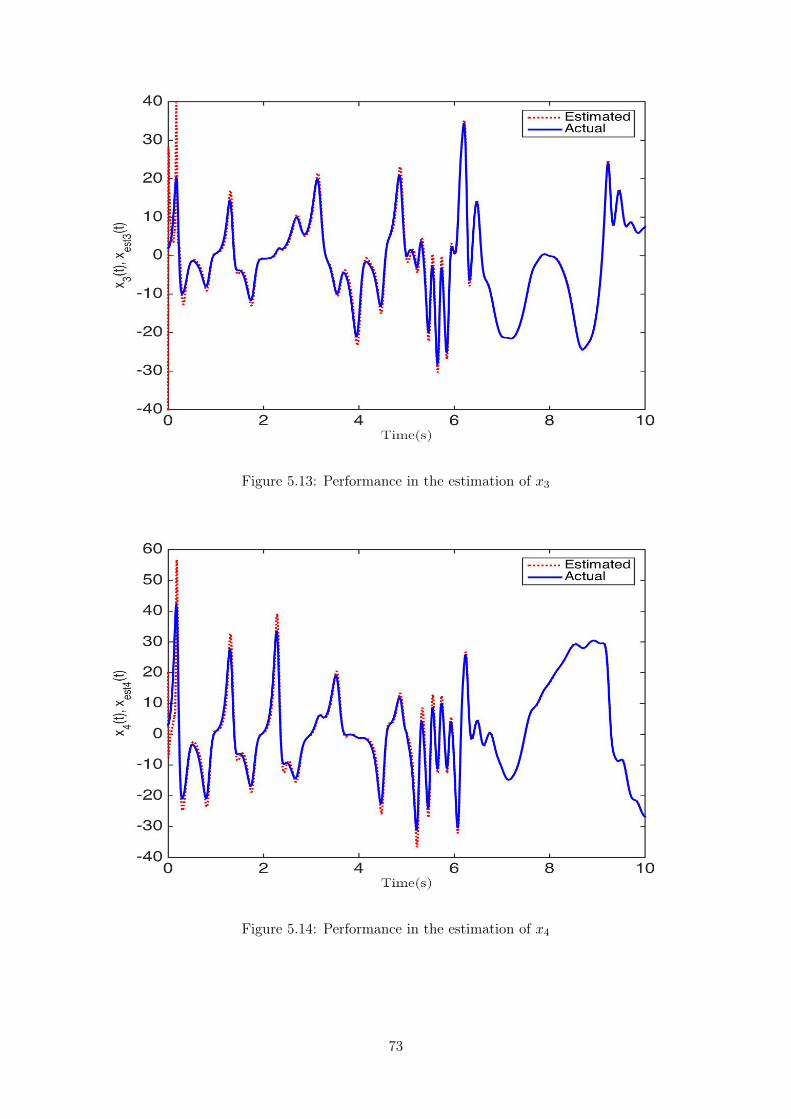
Figure 5.13: Performance in the estimation of x3

Figure 5.14: Performance in the estimation of x4

73

Figure 5.15: Performance in the estimation of x5

Figure 5.16: Performance in the estimation of x6

74

Figure 5.17: Performance in the estimation of x7

Figure 5.18: Frobenius norm of the estimated weight matrix W

75

Figure 5.19: Frobenius norm of the estimated weight matrix V

5.6.3 Comparison with Ref. [2]

To illustrate the advantages of the proposed methodology, the identification model introducedin [2] is used here for comparison. Consider the online identification multilayer neural networkalgorithm proposed in [2] described as

˙

x = Ax+

ˆ

W�

⇣

ˆ

V

ˆ

x

⌘

˙

ˆ

W = �⌘1�

x

TA

�1�T

⇣

�

⇣

ˆ

V

ˆ

x

⌘⌘T� ⇢1kxk ˆ

W

˙

ˆ

V = �⌘2✓

x

TA

�1ˆ

W

✓

I � ¯

⇤

⇣

ˆ

V

ˆ

x

⌘Tˆ

x

T � ⇢2kxk ˆV◆◆

(5.38)

where ¯

⇤

⇣

ˆ

V

ˆ

x

⌘

= diag

n

�

2i

⇣

ˆ

V

ˆ

x

⌘o

. The Chen system (5.30) is considered. The design parametersare chosen as ⌘1 = 25 and ⌘2 = 0.4, ⇢1 = 0.00012, ⇢2 = 0.00012, the sigmoid function is �(.) =500/1 + exp� 0.5(.). The design matrix A is chosen as

A =

2

6

4

�0.0078 0 0

0 �0.0078 0

0 0 �0.0078

3

7

5

(5.39)

Other design parameters and initial conditions were chosen as in section 5.6.1.

We consider the same disturbance from the previous example in (5.33). Figs. 5.20-5.22 show the

76

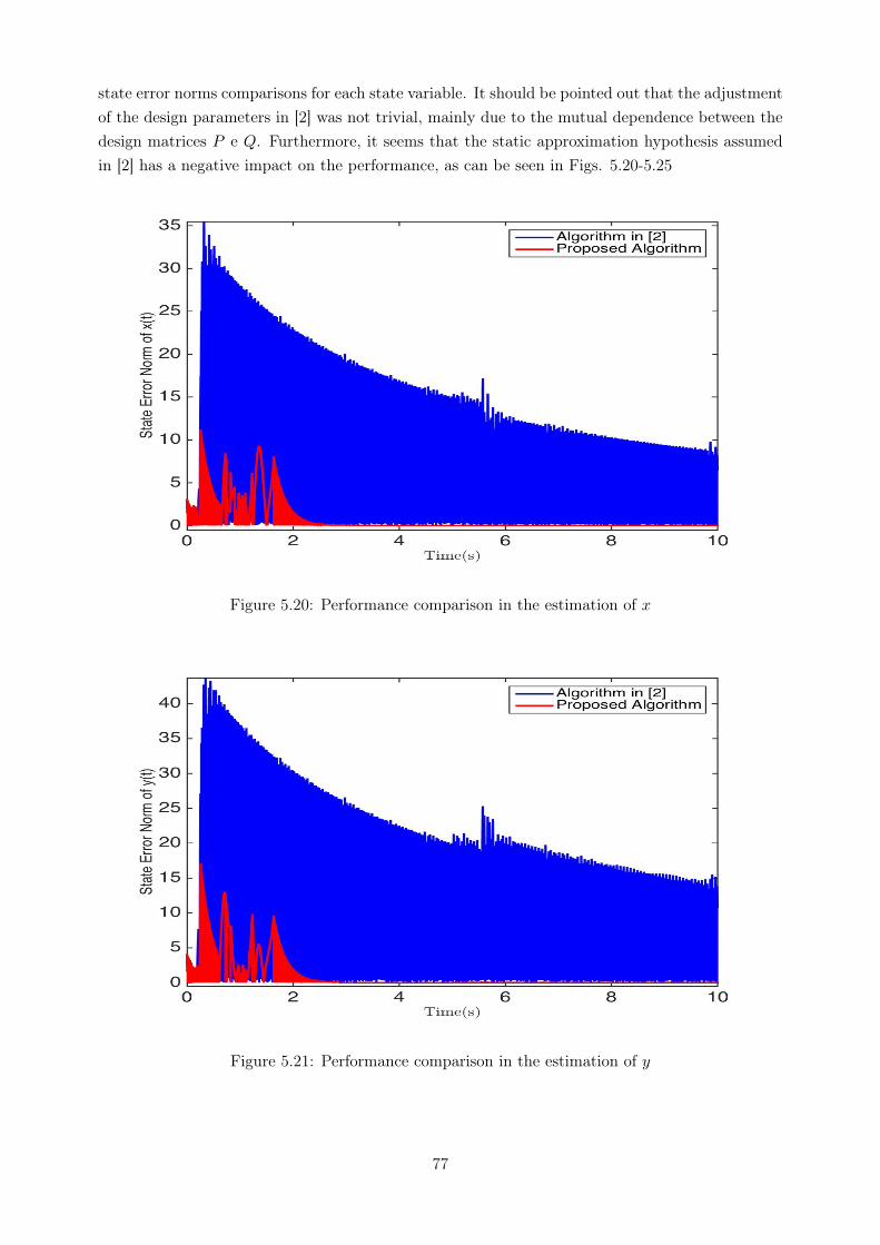
state error norms comparisons for each state variable. It should be pointed out that the adjustmentof the design parameters in [2] was not trivial, mainly due to the mutual dependence between thedesign matrices P e Q. Furthermore, it seems that the static approximation hypothesis assumedin [2] has a negative impact on the performance, as can be seen in Figs. 5.20-5.25

Figure 5.20: Performance comparison in the estimation of x

Figure 5.21: Performance comparison in the estimation of y

77

Figure 5.22: Performance comparison in the estimation of z

Figure 5.23: Frobenius norm of the estimated weight matrix W

78

Figure 5.24: Frobenius norm of the estimated weight matrix V

Figure 5.25: Frobenius norm of the estimated weight matrix W

79

Figure 5.26: Frobenius norm of the estimated weight matrix V

5.7 Discussions

As stated in previous sections, for all the simulations of the proposed algorithms, the designmatrices A, B, P and K were initially chosen as identity matrices. In the sequence, these valueswere adjusted, by a trial and error procedure to fulfill requirements of performance. After atransient phase, due to the large initial uncertainty, these norms seem to converge, indicating thatmost of the state estimation error has been removed. It should be noted that the transient can beshaped according to the user’s desired convergence as well as the learning speed can be adjustedgiven the project requirements.

The transients of the simulations with the algorithm proposed in Chapter 4 showed higherfrequency behavior than the algorithm proposed in this chapter. Although they can be modeled toshow a slower frequency, it is generally easier and more intuitive to shape the transient with SHLNNscheme. However, the trade-off involved is that the former methodology is faster than the lattergiven that only needs tuning for the output weights once the hidden layer is randomly generatedand remains fixed during the simulation. Additionally, despite the heavier computational cost, theSHLNN model required less inputs nodes than the algorithm proposed in Chapter 4, alleviatingthe so called "curse of dimensionality" for linearly parametrized models.

80

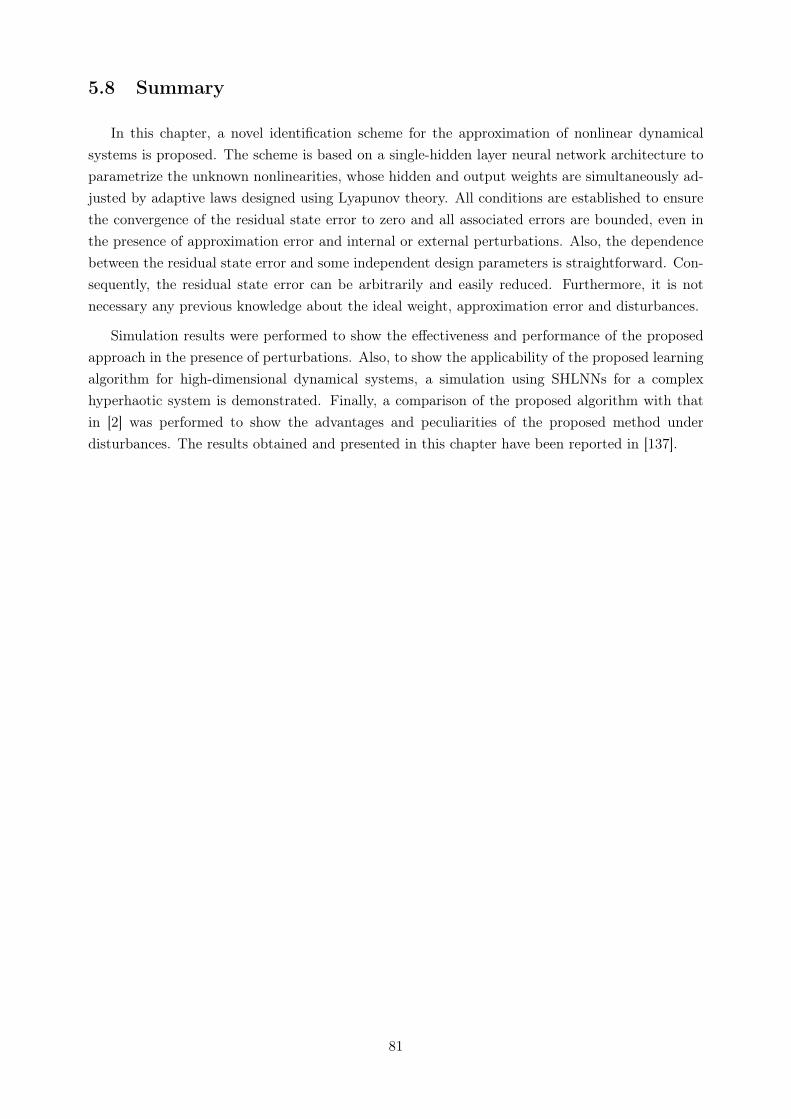
5.8 Summary

In this chapter, a novel identification scheme for the approximation of nonlinear dynamicalsystems is proposed. The scheme is based on a single-hidden layer neural network architecture toparametrize the unknown nonlinearities, whose hidden and output weights are simultaneously ad-justed by adaptive laws designed using Lyapunov theory. All conditions are established to ensurethe convergence of the residual state error to zero and all associated errors are bounded, even inthe presence of approximation error and internal or external perturbations. Also, the dependencebetween the residual state error and some independent design parameters is straightforward. Con-sequently, the residual state error can be arbitrarily and easily reduced. Furthermore, it is notnecessary any previous knowledge about the ideal weight, approximation error and disturbances.

Simulation results were performed to show the effectiveness and performance of the proposedapproach in the presence of perturbations. Also, to show the applicability of the proposed learningalgorithm for high-dimensional dynamical systems, a simulation using SHLNNs for a complexhyperhaotic system is demonstrated. Finally, a comparison of the proposed algorithm with thatin [2] was performed to show the advantages and peculiarities of the proposed method underdisturbances. The results obtained and presented in this chapter have been reported in [137].

81

Chapter 6

Conclusions

This Master’s thesis develops two novel online learning algorithms for neuro-based identificationof a general class of nonlinear dynamical systems. The neuro identifiers were designed based onLyapunov theory to ensure state error convergence to zero, despite the presence of approximationerror and disturbances. This approach demonstrated its capabilities in terms of having a shortdevelopment time and high accuracy, solving complex problems, and possessing the beneficialdesign properties of stability.

Chapter 2 provides a description of the historical developments of system identification alongwith a state of the art review of identification based on single-hidden layer neural networks. Theliterature review shows the relevancy and need for neural learning algorithms in control applicationswhere attributes such as convergence and stability can be verified analytically. Despite successfuluse of neural networks for a wide range of applications, they are prone to local optimal problemand have slow convergence rates which limits itself to relatively simpler problems. In chapter3, technical background about neural networks, their properties and the notation that was usedthroughout this Master’s thesis is introduced. Furthermore, a brief description is given for themost used neural network topologies and the basic types of learning.

Several approaches has been recently proposed in the literature to tackle the aforementionedchallenges. One has been extreme learning machine models which are linearly parametrized modelsefficient in terms of computation as well as optimality. The ELM and its variants lacks the stabilityanalysis and conditions to ensure error boundedness or asymptotical convergence of the state errorto zero. In this context, deriving an ELM-based identification scheme with adaptive output weightsis highly desired. Recent researches based on Lyapunov theory have been proposed to address theseissues [1, 15] by providing error boundedness, however they lack the assurance of asymptoticalconvergence of the residual state error to zero and boundedness of all associated approximationerrors in the presence of approximation error and disturbances.

Aiming to address the above drawbacks. In chapter 4, by using an extreme learning machine, anonline adaptive neuro-identification scheme for a general class of nonlinear systems in the presenceof unknown dynamics and external disturbances is proposed. It is noteworthy that, besides thebounds assumption, no previous knowledge about the dynamics of the approximation error, ideal

82

weights or external perturbations is needed. The ELM is a class of SHLNNs where the hiddenlayer weights are randomly generated according to any continuous probability distribution, andhere the output weights of the ELM are updated based on the stable adaptive laws derived fromLyapunov analysis. Analysis based on Lyapunov theory shows that the adaptive learning algorithmconverges asymptotically for estimation of nonlinear systems with no prior knowledge about theirsystem dynamics and under perturbations. The proposed methodology combines computationalefficiency in terms of learning speed from the ELM technique with the stability of the system underdisturbances guaranteed by the Lyapunov analysis.

Simulation results for a unified chaotic system and a hyperchaotic finance system demonstratedthe effectiveness and performance of the proposed approach in the presence of disturbances. Addi-tionally, to show the efficiency of the proposed learning algorithm for high-dimensional dynamicalsystems, a simulation for a complex hyperhaotic system is demonstrated without compromisingthe learning speed and convergence property. Finally, a comparison of the proposed algorithm withthat in [1] was performed to show the advantages and peculiarities of the proposed method underdisturbances. The state estimation error shows better convergence under external disturbancesand avoids the parameter drift, as the weight norms show nearly constant values.

Further, as a more general case of neural identification, multilayer neural networks presentbetter generalization performance for higher-dimensional problems, alleviating the "curse of di-mensionality" common on linearly parametrized problems. Nevertheless, a considerable share ofproposed learning algorithms for SHLNNs are modifications of gradient descent type algorithms,lacking stability analysis and robust terms to ensure convergence under external disturbances andmay suffer from slow convergence.

Considering the previous limitations, in chapter 5, a novel identification scheme for the ap-proximation of nonlinear dynamical systems is proposed. The scheme is based on a single-hiddenlayer neural network architecture to parametrize the unknown nonlinearities, whose hidden andoutput weights are simultaneously adjusted by adaptive laws designed with Lyapunov theory. Allconditions are established to ensure the convergence of the residual state error to zero and allassociated errors are bounded, even in the presence of approximation error and internal or exter-nal perturbations. Also, the dependence between the residual state error and some independentdesign parameters is straightforward. Consequently, the residual state error can be arbitrarily andeasily reduced. Furthermore, it is not necessary any previous knowledge about the ideal weight,approximation error and disturbances.

Simulation results were performed to show the effectiveness and performance of the proposedapproach in the presence of perturbations. Also, to show the applicability of the proposed learningalgorithm for high-dimensional dynamical systems, a simulation for a complex hyperhaotic systemis demonstrated. Finally, a comparison of the proposed algorithm with that in [2] was performedto show the advantages and peculiarities of the proposed method under disturbances. The stateestimation error shows faster convergence near the origin, as the weight norms show nearly con-stant values, however the main difficulty was heavier computational cost. There are several otheropportunities to extend the present work in the future as below:

83

• The universal approximation capability is an important property since it justifies the appli-cation of the neural networks to any function approximation problem. However, the theoremis not constructive due to the fact that no method is provided for finding the ideal weights,optimum learning time and no information about the number and characteristics of the hid-den neurons that would be required to achieve a given accuracy. Thus, tuning the designparameters of a neural network to a given target performance can be a rather tiresome taskand may lead to sub-optimal solution, specially in identification of nonlinear systems. Forfuture work, applications in evolutionary computation may help alleviate this issue. Sincethey belong to a family of trial and error problem solvers and are mostly applied to blackbox applications, they can be a valuable tool for global dynamic optimization search inidentification of complex nonlinear systems.

• Another issue for identification of nonlinear systems is the need of all inputs for measuring.Nevertheless, this is not often possible in practical situations, since physical sensors typicallyhave shortcomings that can degrade a control system for a number of reasons. To cite afew, sensors may be expensive and substantially raise the cost of a control system, theycan induce significant errors such as limited responsiveness and stochastic noise, also somesignals are impractical to measure given the environment. To mitigate such limitations, itcould be an interesting research direction for the future to investigate the potential of theproposed learning algorithms for observer models. Since observers are considered a generalcase of system identification, they provide better and cheaper implementation in engineeringapplications.

• The simulations included in this Master’s thesis are classified as open-loop identification.However, there are plants which may contain an integrator or are unstable in open-loopoperation. The integrator is an inherently unstable device which tends to make the systemless stable as, for instance, its response to a step input, a bounded signal, is a ramp, aunbounded signal. In many engineering applications, the performance of the closed-loopsystem can be improved by using a controller based on the identified model from the closed-loop data. Thus, further researches could focus on identification for robust control where aplant model is identified in closed-loop operation.

84

References

[1] JANAKIRAMAN, V.; ASSANIS, D. Lyapunov method based online identification of non-linear systems using extreme learning machines. Computing Research Repository (CoRR),abs/1211.1441, p. 1–8, 2012.

[2] ABDOLLAHI, F.; TALEBI, H.; PATEL, R. Stable identification of nonlinear systems usingneural networks: Theory and experiments. IEEE Transactions on Mechatronics, v. 11, n. 4, p.488–495, 2006.

[3] ABLAMEYKO, S. et al. Neural Networks for Instrumentation, Measurement and Related In-dustrial Applications. [S.l.]: IOS Press, 2003.

[4] HAYKIN, S. Neural networks and learning machines. [S.l.]: Pearson Prentice Hall, 2008.

[5] LEONDES, C. Control and Dynamic Systems. [S.l.]: Academic Press, 1997.

[6] LJUNG, L. Perspectives on system identification. Annual Reviews in Control, v. 34, n. 4, p.1–12, 2010.

[7] ZADEH, L. From circuit theory to system theory. IRE Proceedings, v. 50, n. 5, p. 856–865,1962.

[8] TANGIRALA, A. Principles of System Identification: Theory and Practice. [S.l.]: CRC Press,2015.

[9] FU, L.; LI, P. The research survey of system identification method. In: 5th InternationalConference on Intelligent Human-Machine Systems and Cybernetics. [S.l.]: IEEE, 2013. p. 397– 401.

[10] GE, S. et al. Stable Adaptive Neural Network Control. [S.l.]: Springer, 2002.

[11] IOANNOU, P.; SUN, J. Robust adaptive control. [S.l.]: Dover Publications, 2012.

[12] LIU, G. Nonlinear Identification and Control: A Neural Network Approach. [S.l.]: Springer,2001.

[13] HUANG, G.; ZHU, Q.-Y.; SIEW, C.-K. Extreme learning machine: Theory and applications.Neurocomputing, v. 70, p. 489–501, 2006.

85

[14] SUN, J. et al. Extreme learning control of surface vehicles with unknown dynamics and dis-turbances. Neurocomputing, v. 167, n. 1, p. 535–542, 2015.

[15] RONG, H.; ZHAO, G. Direct adaptive neural control of nonlinear systems with extremelearning machine. Neural Comput. and Applic., v. 22, n. 3, p. 577–586, 2013.

[16] TANG, Y.; LI, Z.; GUAN, X. Identification of nonlinear system using extreme learning ma-chine based hammerstein model. Commun. Nonlinear Sci. Numer. Simulat., v. 19, n. 9, p.3171–3182, 2014.

[17] RONG, H. et al. Adaptive neural control for a class of mimo nonlinear systems with extremelearning machine. Neurocomputing, v. 149, p. 405–414, 2015.

[18] JANAKIRAMAN, V.; NGUYEN, X.; ASSANIS, D. Stochastic gradient based extreme learn-ing machines for online learning of advanced combustion engines. Neurocomputing, v. 177, p.304–316, 2016.

[19] BAZAEI, A.; MOALLEM, M. Online neural identification of multi-input multi-output sys-tems. IET Control Theory Applications, v. 1, n. 1, p. 44–50, 2007.

[20] VARGAS, J.; HEMERLY, E. Neural adaptive observer with asymptotic convergence in thepresence of time-varying parameters and disturbances. (in Portuguese) Sba Controle Autom.,v. 19, p. 18–29, 2008.

[21] VARGAS, J.; HEMERLY, E.; VILLARREAL, E. Stability analysis of a neuro-identificationscheme with asymptotic convergence. International Journal of Artificial Intelligence and Appli-cations, v. 3, n. 4, p. 35–50, 2012.

[22] GAUSS, C. Theoria Motus Corporum Coelestium. [S.l.]: Dover Publications, 1809.

[23] DEISTLER, M. System identification and time series analysis. In: Proc. Stochastic Theoryand Control. [S.l.]: Festschrift for Tyrone Duncan, 2002. p. 97–108.

[24] GEVERS, M. A personal view of the development of system identification. IEEE ControlSystems Magazine, v. 26, n. 6, p. 93–105, 2006.

[25] HO, B.; KALMAN, R. Effective contruction of linear state-variable models from input-outputfunctions. Regelungstechnik, v. 12, p. 545–548, 1965.

[26] ASTROM, K.; BOHLIN, T. Numerical identification of linear dynamic systems from normaloperating records. In: Proc. IFAC Symp. Self-Adaptive Systems. [S.l.]: Teddington, U.K., 1992.p. 96–111.

[27] KOOPMANS, T.; RUBIN, H.; LEIPNIK, R. Measuring the equation systems of dynamiceconomics. Cowles Comission Monograph, v. 10, 1950.

[28] HANNAN, E. Time Series Analysis. [S.l.]: Methuen, 1960.

[29] BOX, G.; REINSEL, G. J. aand G. Time Series Analysis: Forecasting and Control. [S.l.]:John Wiley and Sons, 2008.

86

[30] KUNG, S. A new identification method and model reduction algorithm via singular valuedecomposition. In: 12th Asilomar Conf. on Circuits, Systems and Computers. [S.l.]: Asilomar,CA, 1978. p. 705–714.

[31] AKAIKE, H. Stochastic theory of minimal realization. IEEE Transaction on Automation andControl, v. 19, n. 6, p. 667–674, 1974.

[32] LJUNG, L. On consistency and identifiability. Math. Program Study, v. 5, p. 169–190, 1976.

[33] ANDERSON, B.; MOORE, J.; HAWKES, R. Model approximation via prediction error iden-tification. Automatica, v. 14, n. 6, p. 615–622, 1978.

[34] LJUNG, L.; CAINES, P. Asymptotic normality of prediction error estimators for approxima-tive system models. Stochastics, v. 3, p. 29–46, 1979.

[35] LJUNG, L. Convergence analysis of parametric identification methods. IEEE Transactions onAutomatic Control, v. 23, n. 5, p. 770–783, 1978.

[36] LJUNG, L. Asymptotic variance expressions for identified black-box transfer function estima-tion. IEEE Transaction on Automation and Control, v. 30, n. 9, p. 834–844, 1985.

[37] WAHLBERG, B.; LJUNG, L. Design variables for bias estimation in transfer function esti-mation. IEEE Transaction on Automation and Control, v. 31, n. 2, p. 133–144, 1986.

[38] GEVERS, M.; LJUNG, L. Optimal experiment designs with respect to the intended modelapplication. Automatica, v. 22, n. 5, p. 543–554, 1986.

[39] LJUNG, L. System Identification - Theory for the User. [S.l.]: Prentice-Hall, 1999.

[40] POGGIO, T.; GIROSI, F. Regularization algorithms for learning that are equivalent to mul-tilayer networks. Science, v. 247, n. 4945, p. 978–982, 1990.

[41] POGGIO, T.; GIROSI, F. Networks for approximation and learning. Proceedings of the IEEE,v. 78, n. 9, p. 1481–1497, 1990.

[42] ZADEH, L. Fuzzy logic, neural networks, and soft computing. Communication ACM, v. 37,n. 3, p. 77–86, 1994.

[43] WANG, L. Adaptive Fuzzy Systems and Control: Design and Stability Analysis. [S.l.]: PearsonPrentice Hall, 1994.

[44] ZHANG, Q.; BENVENISTE, A. Wavelet networks. IEEE Transactions on Neural Networks,v. 3, n. 6, p. 889–898, 1992.

[45] LIU, G.; BILLINGS, S.; KADIRKAMANATHAN, V. Nonlinear system identification usingwavelet networks. Proceedings of the UKACC International Conference on Control, p. 1248–1253,1998.

87

[46] LIU, G.; BILLINGS, S.; KADIRKAMANATHAN, V. Identification of nonlinear dynamicalsystems using wavelet networks. International Journal of Systems Science, v. 31, p. 1531–1541,2000.

[47] ANTSAKLIS, P. Special issue on neural networks in control systems. IEEE Control SystemsMagazine, v. 10, p. 3–5, 1990.

[48] MILLER, T.; SUTTON, R.; WERBOS, P. Neural Networks for Control. [S.l.]: MIT Press,1990.

[49] CHEN, S.; BILLINGS, S.; GRANT, P. Nonlinear system identification using neural networks.International Journal of Control, v. 51, n. 6, p. 1191–1214, 1990.

[50] NARENDRA, K.; PARTHASARATHY, K. Identification and control of dynamical systemsusing neural networks. IEEE Transactions on Neural Networks, v. 1, n. 1, p. 4–27, 1990.

[51] BILLINGS, S.; CHEN, S. Neural networks and system identification. Neural Networks forSystems and Control, v. 7, p. 181–205, 1992.

[52] QIN, S.; SU, H.; MCAVOY, T. Comparison of four net learning methods for dynamic systemidentification. IEEE Transactions on Neural Networks, v. 3, n. 1, p. 122–130, 1992.

[53] WILLIS, M. et al. Artificial neural networks in process estimation and control. Automatica,v. 28, n. 6, p. 1181–1187, 1992.

[54] KUSCHEWSKI, J.; HUI, S.; ZAK, S. Application of feedforward neural networks to dynamicalsystem identification and control. IEEE Transactions on Control Systems Technology, v. 1, n. 1,p. 37–49, 1993.

[55] POLYCARPOU, M.; IOANNOU, P. Identification and control of nonlinear systems usingneural network models: design and stability analysis. [S.l.], 1991. Tecnical Report 91-09-01.

[56] SANNER, R.; SLOTINE, J. Gaussian networks for direct adaptive control. IEEE Transactionson Neural Networks, v. 3, n. 6, p. 837–863, 1992.

[57] SADEGH, N. A perceptron network for functional identification and control of nonlinearsystems. IEEE Transactions on Neural Networks, v. 4, n. 6, p. 982–988, 1993.

[58] WERBOS, R. Backpropagation through time: what it does and how to do it. Proceedings ofthe IEEE, v. 78, n. 10, p. 1550–1560, 1990.

[59] WILLIAMS, R.; ZIPSER, D. A learning algorithm for continuous running fully recurrentneural networks. Neural Computation, v. 1, n. 2, p. 270–280, 1989.

[60] NARENDRA, K.; PARTHASARATHY, K. Gradient methods for the optimization of dynam-ical systems containing neural networks. IEEE transactions on Neural Networks, v. 2, n. 2, p.252–262, 1991.

[61] NARENDRA, K.; PARTHASARATHY, K. Stable Adaptive Systems. [S.l.]: Prentice-Hall,1989.

88

[62] SLOTINE, J.; LI, W. Applied Nonlinear Control. [S.l.]: Prentice-Hall International, 1991.

[63] BEHERA, L.; KUMAR, S.; PATNAIK, A. On adaptive learning rate that guarantees conver-gence in feedforward networks. IEEE Transactions on Neural Networks, v. 17, n. 5, p. 1116–1125,2006.

[64] MAN, Z. et al. A new adaptive backpropagation algorithm based on lyapunov stability theoryfor neural networks. IEEE Transactions on Neural Networks, v. 17, n. 6, p. 1580–1591, 2006.

[65] YU, X.; EFE, M.; KAYNAK, O. A general backpropagation algorithm for feedforward neuralnetworks learning. IEEE Transactions on Neural Networks, v. 13, n. 1, p. 251–254, 2002.

[66] VARGAS, J.; GULARTE, K.; HEMERLY, E. Online neuro-identification of uncertain systemsbased on scaling and explicit feedback. Control Automation and Electrical Systems, v. 24, n. 6,p. 753–763, 2013.

[67] KOSMATOPOULOS, E. et al. High-order neural network structures for identification of dy-namical systems. IEEE Transactions on Neural Networks, v. 6, n. 2, p. 422–431, 1995.

[68] ABDOLLAHI, F.; TALEBI, H.; PATEL, R. A stable neural network-based observer withapplication to flexible-joint manipulators. IEEE Transactions on Neural Networks, v. 17, n. 1,p. 118–129, 2006.

[69] YU, W.; RUBIO, J. Recurrent neural networks traininng with stable bounding ellipsoid algo-rithm. IEEE Transactions on Neural Networks, v. 20, n. 6, p. 983–991, 2009.

[70] RUBIO, J.; ANGELOV, P.; PACHECO, J. Uniformly stable backpropagation algorithm totrain a feedforward neural network. IEEE Transactions on Neural Networks, v. 22, n. 3, p.356–366, 2006.

[71] HUANG, G. et al. Extreme learning machine for regression and multiclass classification. IEEETransactions on Systems, Man and Cybernetics, v. 42, n. 2, p. 513–529, 2012.

[72] HUANG, G.; BABRI, H. Upper bounds on the number of hidden neurons in feedforwardnetworks with arbitrary bounded nonlinear activation functions. IEEE Transactions on NeuralNetworks, v. 17, n. 1, p. 879–892, 1998.

[73] WANG, Y.; CAO, F.; YUAN, Y. A study on effectiveness of extreme learning machine.Neurocomputing, v. 74, n. 16, p. 2483–2490, 2011.

[74] DING, S. et al. Extreme learning machine: algorithm, theory and applications. Artif. Intell.Rev., v. 44, n. 1, p. 103–115, 2015.

[75] FARREL, J.; POLYCARPOU, M. Adaptive Approximation Based Control: Unifying Neural,Fuzzy and Tradicional Adaptive Approximation Approaches. [S.l.]: Wiley, 2006.

[76] HECHT-NIELSEN, R. Kolmogorov’s mapping neural network existence theorem. First IEEEInternational Conference on Neural Networks, v. 3, p. 11–14, 1987.

89

[77] LIPPMANN, R. An introduction to computing with neural nets. IEEE ASSP Magazine, v. 4,n. 2, p. 4–22, 1987.

[78] SPRECHER, D. On the structure of continuous functions of several variables. Transactionsof the American Mathematical Society, v. 115, p. 340–355, 1965.

[79] GALLANT, A.; WHITE, H. There exists a neural network that does not make avoidablemistakes. Neural Networks, v. 2, p. 657–664, 1989.

[80] CYBENKO, G. Approximation by superpositions of a sigmoidal function. Math. Control Sig-nal Systems, v. 2, n. 4, p. 303–314, 1989.

[81] HORNIK, K.; STINCHCOMBE, M.; WHITE, H. Multilayer feedforward networks are uni-versal approximators. Neural Networks, v. 2, n. 5, p. 359–366, 1989.

[82] FUNAHASHI, K.-I. On the approximate realization of continuous mappings by neural net-works. IEEE International Conference on Neural Networks, v. 1, n. 3, p. 183–192, 1989.

[83] HORNIK, K.; STINCHCOMBE, M.; WHITE, H. Universal approximation of an unknownmapping and its derivatives using multilayer feedforward networks. Neural Networks, v. 3, n. 5,p. 551–560, 1990.

[84] LIGHT, W. Ridge functions, sigmoidal functions and neural networks. In: In ApproximationTheory VII. [S.l.]: Academic Press, 1992. p. 163–206.

[85] SUN, X.; CHENEY, E. The fundamentals of sets of ridge functions. Aequationes Math., v. 44,p. 226–235, 1992.

[86] STINCHCOMBE, M.; WHITE, H. Universal approximation using feedforward networks withnon-sigmoid hidden layer activation functions. In: International Joint Conference on NeuralNetworks. [S.l.: s.n.], 1989. v. 1, p. 613–617.

[87] HORNIK, K. Approximation capabilities of multilayer feedforward networks. Neural Networks,v. 4, n. 2, p. 251–257, 1991.

[88] LESHNO, M. et al. Multilayer feedforward networks with a nonpolynomial activation functioncan approximate any function. Neural Networks, v. 6, n. 6, p. 861–867, 1993.

[89] HORNIK, K. Some new results on neural network approximation. Neural Networks, v. 6, n. 8,p. 1069–1072, 1993.

[90] KULAKOV, A.; ZWOLINSKI, M.; REEVE, J. Fault tolerance in distributed neural comput-ing. ArXiv e-prints, v. 1509.09199, 2015.

[91] ROSENBLATT, F. The perceptron: A probabilistic model for information storage and orga-nization in the brain. Psychological Review, v. 65, p. 386–408, 1958.

[92] HEBB, D. The Organization of Behavior: A Neuropsychological Theory. [S.l.]: Wiley, 1949.

90

[93] MINSKY, M.; SELFRIDGE, O. Learning in random nets. In: Information Theory. [S.l.]: 4thLondom Symposium, 1961.

[94] RUMELHART, D.; HINTON, G.; WILLIAMS, R. Learning internal representations by errorpropagation. Parallel Distributed Processing, v. 1, p. 318–362, 1986.

[95] BENGIO, Y. Learning deep architectures for a.i. Foundations and Trends in Machine Learn-ing, v. 2, p. 1–127, 2009.

[96] BENGIO, Y.; COURVILLE, A. C.; VINCENT, P. Unsupervised feature learning and deeplearning: A review and new perspectives. CoRR, abs/1206.5538, 2012.

[97] SCHMIDHUBER, J. Deep learning in neural networks: An overview. Neural Networks, v. 61,p. 85–117, 2015.

[98] KARAYIANNIS, N.; VENETSANOPOULOS, A. Artificial Neural Networks: Learning Algo-rithms, Performance Evaluation and Applications. [S.l.]: Springer, 1993.

[99] GILES, C.; MAXWELL, T. Learning, invariance, and generalization in higher order neuralnetworks. Applied Optics, v. 26, n. 23, p. 4972–4978, 1987.

[100] PARETTO, P.; NIEZ, J. Long term memory storage capacity of multiconnected neuralnetworks. Biological Cybernetics, v. 54, p. 53–63, 1986.

[101] REDDING, N.; KOWALCZYK, A.; DOWNS, T. Constructive high-order network algorithmthat is polynomial time. Neural Networks, v. 6, n. 7, p. 997–1010, 1993.

[102] ESTEVEZ, P.; OKABE, Y. Training the piecewise linear-high order neural network througherror back propagation. In: Proceedings of IEEE International Joint Conference on Neural Net-works,. [S.l.: s.n.], 1991. v. 1, p. 771–716.

[103] SPIRKOVSKA, L.; REID, M. Robust position, scale, and rotation invariant object recogni-tion using higher-order neural networks. Pattern Recognition, v. 25, n. 9, p. 975–985, 1992.

[104] PARK, J.; SANDBERG, I. Universal approximation using radial-basis-function networks.Neural Computation, v. 3, n. 2, p. 246–257, 1990.

[105] HARTMAN, E.; KEELER, J.; KOWALSKI, J. Layered neural networks with gaussian hiddenunits as universal approximations. Neural Computation, v. 2, n. 2, p. 210–215, 1990.

[106] HUSH, D.; HORNE, B. Progress in supervised neural networks. IEEE Signal ProcessingMagazine, v. 10, n. 1, p. 8–39, 1993.

[107] ZADEH, L. Outline of a new approach to the analysis of complex systems and decisionprocesses. IEEE Transactions on Systems, Man, and Cybernetics, v. 3, n. 1, p. 28–44, 1973.

[108] WANG, L. X.; MENDEL, J. M. Fuzzy basis functions, universal approximation, and or-thogonal least-squares learning. IEEE Transactions on Neural Networks, v. 3, n. 5, p. 807–814,1992.

91

[109] KOSKO, B. Neural Networks and Fuzzy Systems. [S.l.]: Pearson Prentice Hall, 1992.

[110] JANG, J.-S.; SUN, C.; MIZUTANI, E. Functional equivalence between radial basis functionnetworks and fuzzy inference systems. IEEE Transactions on Neural Networks, v. 4, n. 1, p.156–159, 1993.

[111] KECMAN, V.; PFEIFFER, B.-M. Exploiting the structural equivalence of learning fuzzysystems and radial basis function networks. In: European Congress on Intelligent Techniquesand Soft Computing (EUFIT). [S.l.]: Aachen, Germany, 1994. p. 58–66.

[112] NELLES, O. Nonlinear system identification: from classical approaches to neural networksand fuzzy models. [S.l.]: Springer, 2001.

[113] BARUCH, I. et al. A fuzzy-neural multi-model for nonlinear systems identification and con-trol. Fuzzy Sets and Systems, v. 159, n. 20, p. 2650–2667, 2008.

[114] YU, L.; ZHANG, Y. Evolutionary fuzzy neural networks for hybrid financial prediction.IEEE Transactions on Systems, Man and Cybernetics, v. 35, n. 2, p. 244–249, 2005.

[115] THEODORIDIS, D.; BOUTALIS, Y.; CHRISTODOULOU, M. Neuro-fuzzy direct adaptivecontrol of unknown nonlinear systems with analysis on the model order problem. Journal ofZhejiang University, v. 12, p. 1–16, 2011.

[116] CALDERON, A.; ZYGMUND, A. On existence of certain singular integral. Acta Mathemat-ics, v. 88, p. 85–139, 1952.

[117] STRICHARTZ, R. How to make wavelets. American Mathematical Monthly, v. 100, n. 6, p.539–556, 1993.

[118] RIOUL, O.; VETTERLI, M. Wavelets and signal processing. IEEE Signal Processing Mag-azine, v. 8, n. 4, p. 14–38, 1991.

[119] KREINOVICH, V.; SIRISAENGTAKSIN, O.; CABRERA, S. Wavelet neural networks areasymptotically optimal approximators for functions of one variable. In: IEEE World Congresson Computational Intelligence. [S.l.: s.n.], 1994. v. 1, p. 299–304 vol.1.

[120] BILLINGS, S.; WEI, H. A new class of wavelet networks for nonlinear system identification.IEEE Transactions on Neural Networks, v. 16, n. 4, p. 862–874, 2005.

[121] SJOBERG, J. et al. Nonlinear black-box modelling in system identification: a unifiedoverview. Automatica, v. 31, n. 12, p. 1691–1724, 1995.

[122] KUMAR, P.; FOUFOULA-GEORGIOU, E. Multicomponent decomposition of spatial rain-fall fields: segregation of large and small scale features using wavelet transforms. Water ResourcesResearch, v. 29, n. 8, p. 2515–2532, 1993.

[123] ZHANG, Q. Learning algorithm of wavelet network based on sampling theory. Neurocomput-ing, v. 71, n. 1-3, p. 224–269, 2007.

92

[124] PANY, P.; GHOSHAL, S. Application of local linear wavelet neural network in short termelectric load forecasting. International Journal of Computer Applications, v. 51, n. 13, 2012.

[125] CHEN, Y.; YANG, B.; DONG, J. Time-series prediction using a local linear wavelet neuralwavelet. Neurocomputing, v. 69, n. 4-6, p. 449–465, 2006.

[126] WAI, R.; CHANG, H. Backstepping wavelet neural network control for indirect field-orientedinduction motor drive. IEEE Transactions on Neural Networks, v. 15, n. 2, p. 367–382, 2004.

[127] HUANG, G.; WANG, D.; LUAN, Y. Extreme learning machine: Theory and applications.International Journal of Machine Learning and Cybernetics, v. 2, n. 1-3, p. 107–122, 2011.

[128] SUN, F. et al. Extreme Learning Machines 2013: Algorithms and Applications. [S.l.]:Springer, 2014.

[129] KAELBLING, L.; LITTMAN, M.; MOORE, A. Reinforcement learning: A survey. Journalof Artificial Intelligence Research, v. 4, p. 237–285, 1996.

[130] ASTROM, K.; WITTENMARK, P. Adaptive Control. [S.l.]: Addison-Wesley, 1995.

[131] ZHAO, G. et al. On improving the conditioning of extreme learning machine: A linear case.7th International Conference on Information, Communications and Signal Processing, p. 1–5,2009.

[132] Lü, J.; CHEN, D.; CELIKOVSKY, S. Bridge the gap between the lorenz system and chensystem. International Journal of Bifurcation and Chaos, v. 12, n. 12, p. 2917–2926, 2002.

[133] YU, H.; CAI, G.; LI, Y. Dynamic analysis and control of a new hyperchaotic finance system.Nonlinear Dynamics, v. 67, n. 3, p. 2171–2182, 2012.

[134] MAHMOUD, E. Dynamics and synchronization of new hyperchaotic complex lorenz system.Mathematical and Computer Modeling, v. 55, n. 7-8, p. 1951–1962, 2012.

[135] GRZEIDAK, E.; VARGAS, J.; ALFARO, S. Online neuro-identification of nonlinear sys-tems using extreme learning machine. In: Accepted in International Joint Conference on NeuralNetworks IJCNN. [S.l.]: Vancouver, Canada, 2016.

[136] BARRON, A. Universal approximation bounds for superpositions of a sigmoidal function.IEEE Transactions on Information Theory, v. 39, n. 3, p. 930–945, 1993.

[137] VARGAS, J.; GRZEIDAK, E.; ALFARO, S. Identification of unknown nonlinear systemsbased on multilayer neural networks and lyapunov theory. In: Submitted to IEEE Multi-Conference on Systems and Control. [S.l.]: Buenos Aires, Argentina, 2016.

93

Appendix

94

I. CODES

I.1 Appendix 1 - Simulink plant used for simulations correspond-ing to Fig. 4.1-4.17 and Fig. 5.1-5.19

I.2 Appendix 2 - Code for plant model corresponding to Fig. 4.1-4.4

function [sys,x0,str,ts] = Plant(t,x,u,flag)

%Unified Chaotic System

a=1; %Constant for the Chen System

switch flag,

%%%%%%%%%%%%%%%%%%

% Initialization %

%%%%%%%%%%%%%%%%%%

case 0,

sizes = simsizes;

sizes.NumContStates = 3; %Number of Continuous States

sizes.NumDiscStates = 0; %Number of Discret States

sizes.NumOutputs = 3; %Number of Outputs

sizes.NumInputs = 0; %Number of Inputs

sizes.DirFeedthrough = 1;

sizes.NumSampleTimes = 1;

sys = simsizes(sizes);

x0=[�1.5 �2 �5]; %Initial Conditions

str=[];

ts=[0 0];

%%%%%%%%%%%%%%%

95

% Directives %

%%%%%%%%%%%%%%%

case 1,

%Unified chaotic system implementation, the chosen constant

%generates a Chen system.

sys = [(25*a+10)*(x(2)�x(1));(28�35*a)*x(1)�x(1)*x(3)+(29*a�1)*x(2);x(1)*x(2)�((a+8)/3)*x(3)]+disturb(x,u,t);

%%%%%%%%%%

% output %

%%%%%%%%%%

case 3,

sys = x;

%%%%%%%%%%%%%

% End %

%%%%%%%%%%%%%

case {2,4,9},

sys = [];

otherwise

error(['unhandled flag = ',num2str(flag)]);

end

%%%%%%%%%%%%%%%%%%%%%%%%%%%%%%%%%%%%%%%%%%%%%%%%%%%%%%%%%%%%%%%%

%Summary: Return the system's perturbations

%Arguments: state vector, input vector and time

function disturb = disturb(x,u,t)

if t>=5

disturb=[3*sin(7*t)*norm(x(1:3));

10*cos(9*t)*x(1);

(cos(20*t)+10*exp(�t))];else

disturb=0; %Until t=5 secs the disturb is null

end

I.3 Appendix 3 - Code for identifier corresponding to Fig. 4.1-4.4

%Project description: Online Identification using hidden layer neural networks

% with adaptive laws

%Authors: Jose Alfredo Ruiz Vargas and Emerson Grzeidak

%Date: 04/2016 Local: University of Brasilia

function [sys,x0,str,ts] = iden_Caos(t,x,u,flag)

%Diagonal matrix A with negative elements

A = [�10.5 0 0; 0 �9 0; 0 0 �9.5];

%Diagonal matrix A with positive elements

B = 100*[4.1 0 0; 0 3.9 0; 0 0 4];

96

%Constant parameters for learning laws

gammaW=0.001;

gamma0 = 0.1;

gamma1 = 1;

gamma2 = 0.00001;

%Adjustment weights to the output layer

W0 = [0 0 0; 0 0 0; 0 0 0];

%Random generated matrix used for this simulation

%The matrix was generated using V0 = randn(3, 7)

%and the kept fixed for the simulation

V0 = [0.8442 0.8963 0.0968 0.3392 0.1062 0.5720 0.8575;

0.9299 0.5364 0.2585 0.0694 0.8221 0.3607 0.2315;

0.2341 0.2986 0.3643 0.5960 0.5773 0.7750 0.0110];

%Positive definite matrix P and matrix K

P = 500*[0.001 0 0; 0 0.001 0; 0 0 0.001];

K = P + P';

%Parameters for the sigmoidal function

alpha=100;

beta=1;

switch flag,

%%%%%%%%%%%%%%%%%%

% Initialization %

%%%%%%%%%%%%%%%%%%

case 0,

sizes = simsizes;

sizes.NumContStates = 12; %Number of continuous states

sizes.NumDiscStates = 0; %Number of discrete states

sizes.NumOutputs = 16; %Number of outputs

sizes.NumInputs = 3; %Number of inputs

sizes.DirFeedthrough = 1;

sizes.NumSampleTimes = 1;

sys = simsizes(sizes);

x0=zeros(12,1); %Initial conditions

x0(1:3)=5; %Initial conditions for the estimated states

str=[];

ts=[0 0];

%%%%%%%%%%%%%%%

% Directives %

%%%%%%%%%%%%%%%

case 1,

%Identification model and learning laws implementation

97

sys = [A*x(1:3) + B*[x(4:6)'; x(7:9)'; x(10:12)']*Sig(x, u, alpha, beta, ...

V0)�parameter_l(x, u, gamma0, gamma1, gamma2, K, t);

�gammaW*(norm(x_error(x, u))*W_error(x, W0, 1) + w_term1(x, u, B, K, ...

1, alpha, beta, V0));

�gammaW*(norm(x_error(x, u))*W_error(x, W0, 2) + w_term1(x, u, B, K, ...

2, alpha, beta, V0));

�gammaW*(norm(x_error(x, u))*W_error(x, W0, 3) + w_term1(x, u, B, K, ...

3, alpha, beta, V0))];

%%%%%%%%%%%%%%%

% Outputs %

%%%%%%%%%%%%%%%

case 3,

sys = [x(1:12);

norm(x(4:12));

norm((u(1)�x(1)));norm((u(2)�x(2)));norm((u(3)�x(3)))];

case {2,4,9},

sys = [];

otherwise

error(['unhandled flag = ',num2str(flag)]);

end

%%%%%%%%%%%%%%%%%%%%%%%%%%%%%%%%%%%%%%%%%%%%%%%%%%%%%%%%%%%%%%%

%Summary: Return the line of the matrix of estimation errors for the parameter W

%Arguments: state vector, initial weights for W and the desired line

function W_error = W_error(x, W0, line)

%The state vector is in column format, your transposed is needed

%to mount the estimation matrix W

temp = [x(4:6)'; x(7:9)'; x(10:12)'] � W0;

if line == 1

W_error = temp(1,:)';

end

if line == 2

W_error = temp(2,:)';

end

if line == 3

W_error = temp(3,:)';

end

%%%%%%%%%%%%%%%%%%%%%%%%%%%%%%%%%%%%%%%%%%%%%%%%%%%%%%%%%%%%%%%

%Summary: Return the vector function l

%Arguments: state vector, system inputs, matrix K, time t and

%control parameters: gamma0, gamma1, gamma2

function parameter_l = parameter_l(x, u, gamma0, gamma1, gamma2, K, t)

denominator=(min(eig(K))*(norm(x_error(x,u))+gamma1*exp(�gamma2*t)));

98

parameter_l = � (gamma0*x_error(x,u))/denominator;

%%%%%%%%%%%%%%%%%%%%%%%%%%%%%%%%%%%%%%%%%%%%%%%%%%%%%%%%%%%%%%%

%Summary: Return a vector with estimated state's errors

%Arguments: state vector, system inputs

function x_error = x_error(x, u)

X = [x(1); x(2); x(3)];

U = [u(1); u(2); u(3)];

x_error = X � U;

%%%%%%%%%%%%%%%%%%%%%%%%%%%%%%%%%%%%%%%%%%%%%%%%%%%%%%%%%%%%%%%

%Summary: Return the NN's nonlinear regressor vector

%Arguments: state vector, system inputs and sigmoidal function parameters

function Sig = Sig(x,u, alpha, beta, V0) %Regressor

%Parameters for the activation function

V0Z = V0*[u(1); u(2); u(3); u(1)^2; u(2)^2; u(3)^2; 1];

%A sigmoidal function is used, we pass each of the elements of the vector

Sig=[(z(V0Z(1), alpha, beta));

(z(V0Z(2), alpha, beta));

(z(V0Z(3), alpha, beta))];

%%%%%%%%%%%%%%%%%%%%%%%%%%%%%%%%%%%%%%%%%%%%%%%%%%%%%%%%%%%%%%%

%Summary: Sigmoidal fucntion that returns the results of the regressor

%Arguments: the product VZ and parameters for the sigmoidal function

function z = z(arg, alpha, beta) %Sigmoidal activation function

z=alpha/(1+exp(�beta*arg)); %Sigmoidal Function

%%%%%%%%%%%%%%%%%%%%%%%%%%%%%%%%%%%%%%%%%%%%%%%%%%%%%%%%%%%%%%%

%Summary: Return the line of B*K*Xerror*S(VZ)

%Arguments: state vector, system inputs, matrix B and K,

%desired line of the matrix and parameters of sigmoidal function

function w_term1 = w_term1(x, u, B, K, line, alpha, beta, V0)

%term B*K*Xerror*S(VZ) 3x3

temp = B*K*x_error(x,u)*(Sig(x,u, alpha, beta, V0)');

if line == 1

w_term1 = temp(1, :)';

end

if line == 2

w_term1 = temp(2, :)';

end

if line == 3

99

w_term1 = temp(3, :)';

end

I.4 Appendix 4 - Code to display the Fig. 4.1-4.4

%Displays the actual states and their estimations

fsize=22;

figure;

plot(t,x(:,1),'��',t,Xestimated(:,1),'LineWidth',2); set(0,'DefaultAxesFontSize', ...

17);

h=legend('Sistema Caotico','NN');

set(h,'FontSize',fsize);

xlabel('Tempo(s)','Fontsize',fsize);

ylabel('x_{1}(t), x_{NN1}(t)','Fontsize',fsize);

figure;

plot(t,x(:,2),'��',t,Xestimated(:,2),'LineWidth',2); set(0,'DefaultAxesFontSize', ...

17);

h=legend('Sistema Caotico','NN');

set(h,'FontSize',fsize); xlabel('Tempo(s)','interpreter','latex','Fontsize',fsize);

ylabel('x_{2}(t), x_{NN2}(t)','Fontsize',fsize);

figure;

plot(t,x(:,3),'��',t,Xestimated(:,3),'LineWidth',2); set(0,'DefaultAxesFontSize', ...

17);

h=legend('Sistema Caotico','NN');

set(h,'FontSize',fsize);

xlabel('Tempo(s)','Fontsize',fsize);

ylabel('x_{3}(t), x_{NN3}(t)','Fontsize',fsize);

figure;

plot(t,Xestimated(:,13),'LineWidth',1);

set(0,'DefaultAxesFontSize', 17);

set(h,'FontSize',fsize);

xlabel('Tempo(s)','Fontsize',fsize);

ylabel('Estimated Weight Norm W','Fontsize',fsize);

I.5 Appendix 5 - Code for plant model corresponding to Fig. 4.5-4.9

function [sys,x0,str,ts] = Plant(t,x,u,flag)

%Hypercaotic Finance System

100

%Constants for the hyperchaotic system

a=0.9;

b=0.2;

c=1.2;

d=0.17;

k=0.17;

switch flag,

%%%%%%%%%%%%%%%%%%

% Initialization %

%%%%%%%%%%%%%%%%%%

case 0,

sizes = simsizes;

sizes.NumContStates = 4; %Number of continuous states

sizes.NumDiscStates = 0; %Number of discret states

sizes.NumOutputs = 4; %Number of outputs

sizes.NumInputs = 0; %Number of inputs

sizes.DirFeedthrough = 1;

sizes.NumSampleTimes = 1;

sys = simsizes(sizes);

x0=[1 2.5 0.5 0.5]; %Initial conditions

str=[];

ts=[0 0];

%%%%%%%%%%%%%%%

% Directives %

%%%%%%%%%%%%%%%

case 1,

%Unified chaotic system implementation, the chosen constant generates

%a Chen system.

sys = [x(3)+(x(2)�a)*x(1)+x(4);1�b*x(2)�x(1)*x(1);�x(1)�c*x(3);�d*x(1)*x(2)�k*x(4)]+disturb(x,u,t);

%%%%%%%%%%

% Output %

%%%%%%%%%%

case 3,

sys = x;

%%%%%%%%%%%%%

% End %

%%%%%%%%%%%%%

case {2,4,9},

sys = [];

otherwise

error(['unhandled flag = ',num2str(flag)]);

end

%%%%%%%%%%%%%%%%%%%%%%%%%%%%%%%%%%%%%%%%%%%%%%%%%%%%%%%%%%%%%%%

%Summary: Return the system's perturbations

%Arguments: state vector, input vector and time

101

function disturb = disturb(x,u,t)

if t>=5

disturb=[8*sin(7*t)*x(4);

10*cos(9*t)*x(1)*x(1);

x(2)*(cos(20*t)+5*exp(�t));2*sin(20*t)+3*cos(15*t)];

else

disturb=0; %Until t=5 secs the disturb is null

end

I.6 Appendix 6 - Code for identifier corresponding to Fig. 4.5-4.9

%Project description: Online Identification using hidden layer neural networks

% with adaptive laws

%Authors: Jose Alfredo Ruiz Vargas and Emerson Grzeidak

%Date: 04/2015 Local: University of Brasilia

function [sys,x0,str,ts] = iden_Caos(t,x,u,flag)

%Diagonal matrix A with negative elements

A = [�29 0 0 0; 0 �30.5 0 0; 0 0 �30 0; 0 0 0 �28];

%Diagonal matrix A with positive elements

B = 100*[1.1 0 0 0; 0 0.8 0 0; 0 0 1.2 0; 0 0 0 1];

%Constant parameters for the learning laws

gammaW=0.01;

gamma0 = 0.1;

gamma1 = 1;

gamma2 = 0.0001;

%Adjustment weights to the output layer

W0 = [0 0 0 0; 0 0 0 0; 0 0 0 0; 0 0 0 0];

%Random generated matrix used for this simulation

%The matrix was generated using V0 = randn(4, 9)

%and the kept fixed for the simulation

V0 = [0.5377 0.3188 0.5784 0.7254 0.1241 0.6715 0.4889 0.2939 0.0689;

0.8339 0.3077 0.7694 0.0631 0.4897 0.2075 0.0347 0.7873 0.8095;

0.2588 0.4336 0.3499 0.7147 0.4090 0.7172 0.7269 0.8884 0.9443;

0.8622 0.3426 0.0349 0.2050 0.4172 0.6302 0.3034 0.1471 0.4384];

%Positive definite matrix P and Matrix K

P = 50*[0.001 0 0 0; 0 0.001 0 0; 0 0 0.001 0; 0 0 0 0.001];

K = P + P';

%Parameters for the sigmoidal function

102

alpha=150;

beta=1;

switch flag,

%%%%%%%%%%%%%%%%%%

% Initialization %

%%%%%%%%%%%%%%%%%%

case 0,

sizes = simsizes;

sizes.NumContStates = 20; %Number of continuous states

sizes.NumDiscStates = 0; %Number of discrete states

sizes.NumOutputs = 25; %Number of outputs

sizes.NumInputs = 4; %Number of inputs

sizes.DirFeedthrough = 1;

sizes.NumSampleTimes = 1;

sys = simsizes(sizes);

x0=zeros(20,1); %Initial conditions

x0(1:4)=[�2 �2 �2 �2]; %Initial conditions for the estimated states

str=[];

ts=[0 0];

%%%%%%%%%%%%%%%

% Directives %

%%%%%%%%%%%%%%%

case 1,

% Identification model and learning laws implementation

sys = [A*x(1:4) + B*[x(5:8)'; x(9:12)'; x(13:16)'; x(17:20)']*Sig(x, u, ...

alpha, beta, V0)�parameter_l(x, u, gamma0, gamma1, gamma2, K, t);

�gammaW*(norm(x_error(x, u))*W_error(x, W0, 1) + w_term1(x, u, B, K, ...

1, alpha, beta, V0));

�gammaW*(norm(x_error(x, u))*W_error(x, W0, 2) + w_term1(x, u, B, K, ...

2, alpha, beta, V0));

�gammaW*(norm(x_error(x, u))*W_error(x, W0, 3) + w_term1(x, u, B, K, ...

3, alpha, beta, V0));

�gammaW*(norm(x_error(x, u))*W_error(x, W0, 4) + w_term1(x, u, B, K, ...

4, alpha, beta, V0))];

%%%%%%%%%%%%%%%

% Outputs %

%%%%%%%%%%%%%%%

case 3,

sys = [x(1:20);

norm(x(5:20));

norm((u(1)�x(1)));norm((u(2)�x(2)));norm((u(3)�x(3)));norm((u(4)�x(4)))];

case {2,4,9},

103

sys = [];

otherwise

error(['unhandled flag = ',num2str(flag)]);

end

%%%%%%%%%%%%%%%%%%%%%%%%%%%%%%%%%%%%%%%%%%%%%%%%%%%%%%%%%%%%%%%

%Summary: Return the line of the matrix of estimation errors for the parameter W

%Arguments: state vector, initial weights for W and the desired line

function W_error = W_error(x, W0, line)

%The state vector is in column format, your transposed is needed

%to mount the estimation matrix W

temp = [x(5:8)'; x(9:12)'; x(13:16)'; x(17:20)'] � W0;

if line == 1

W_error = temp(1,:)';

end

if line == 2

W_error = temp(2,:)';

end

if line == 3

W_error = temp(3,:)';

end

if line == 4

W_error = temp(4,:)';

end

%%%%%%%%%%%%%%%%%%%%%%%%%%%%%%%%%%%%%%%%%%%%%%%%%%%%%%%%%%%%%%%

%Summary: Return the vector function l

%Arguments: state vector, system inputs, matrix K, time t and control

%parameters: gamma0, gamma1, gamma2

function parameter_l = parameter_l(x, u, gamma0, gamma1, gamma2, K, t)

denominator = (min(eig(K))*(norm(x_error(x,u))+gamma1*exp(�gamma2*t)));parameter_l = � (gamma0*x_error(x,u))/denominator;

%%%%%%%%%%%%%%%%%%%%%%%%%%%%%%%%%%%%%%%%%%%%%%%%%%%%%%%%%%%%%%%

%Summary: Return a vector with estimated state's errors

%Arguments: state vector, system inputs

function x_error = x_error(x, u)

X = [x(1); x(2); x(3); x(4)];

U = [u(1); u(2); u(3); u(4)];

x_error = X � U;

%%%%%%%%%%%%%%%%%%%%%%%%%%%%%%%%%%%%%%%%%%%%%%%%%%%%%%%%%%%%%%%

%Summary: Return the NN's nonlinear regressor vector

%Arguments: state vector, system inputs and sigmoidal function parameters

104

function Sig = Sig(x,u, alpha, beta, V0) %Regressor

%Parameters for the activation function

V0Z = V0*[u(1); u(2); u(3); u(4); u(1)^2; u(2)^2; u(3)^2; u(4)^2; 1];

%A sigmoidal function is used, we pass each of the elements of the vector

Sig=[(z(V0Z(1), alpha, beta));

(z(V0Z(2), alpha, beta));

(z(V0Z(3), alpha, beta));

(z(V0Z(4), alpha, beta))];

%%%%%%%%%%%%%%%%%%%%%%%%%%%%%%%%%%%%%%%%%%%%%%%%%%%%%%%%%%%%%%%

%Summary: Sigmoidal fucntion that returns the results of the regressor

%Arguments: the product VZ and parameters for the sigmoidal function

function z = z(arg, alpha, beta) %Sigmoidal activation function

z=alpha/(1+exp(�beta*arg)); %Sigmoidal Function

%%%%%%%%%%%%%%%%%%%%%%%%%%%%%%%%%%%%%%%%%%%%%%%%%%%%%%%%%%%%%%%

%Summary: Return the line of B*K*Xerror*S(VZ)

%Arguments: state vector, system inputs, matrix B and K,

%desired line of the matrix and parameters of sigmoidal function

function w_term1 = w_term1(x, u, B, K, line, alpha, beta, V0)

%term B*K*Xerror*S(VZ) 3x3

temp = B*K*x_error(x,u)*(Sig(x,u, alpha, beta, V0)');

if line == 1

w_term1 = temp(1, :)';

end

if line == 2

w_term1 = temp(2, :)';

end

if line == 3

w_term1 = temp(3, :)';

end

if line == 4

w_term1 = temp(4, :)';

end

I.7 Appendix 7 - Code to display the Fig. 4.5-4.9

%Displays the actual states and their estimations

fsize=22;

figure;

105

plot(t,x(:,1), '��',t,Xestimated(:,1),'LineWidth',2);set(0,'DefaultAxesFontSize',17);h=legend('Sistema Caotico','NN');

set(h,'FontSize',fsize);

xlabel('Tempo(s)','Fontsize',fsize);

ylabel('x_{1}(t), x_{NN1}(t)','Fontsize',fsize);

figure;

plot(t,x(:,2), '��',t,Xestimated(:,2),'LineWidth',2);set(0,'DefaultAxesFontSize',17);h=legend('Sistema Caotico','NN');

set(h,'FontSize',fsize); xlabel('Tempo(s)','interpreter','latex','Fontsize',fsize);

ylabel('x_{2}(t), x_{NN2}(t)','Fontsize',fsize);

figure;

plot(t,x(:,3), '��',t,Xestimated(:,3),'LineWidth',2);set(0,'DefaultAxesFontSize',17);h=legend('Sistema Caotico','NN');

set(h,'FontSize',fsize);

xlabel('Tempo(s)','Fontsize',fsize);

ylabel('x_{3}(t), x_{NN3}(t)','Fontsize',fsize);

figure;

plot(t,x(:,4),'��',t,Xestimated(:,4),'LineWidth',2);set(0,'DefaultAxesFontSize',17);h=legend('Sistema Caotico','NN');

set(h,'FontSize',fsize);

xlabel('Tempo(s)','Fontsize',fsize);

ylabel('x_{4}(t), x_{NN4}(t)','Fontsize',fsize);

figure;

plot(t, Xestimated(:,21), 'LineWidth', 1 );

set(0,'DefaultAxesFontSize', 17);

set(h,'FontSize',fsize);

xlabel('Tempo(s)','Fontsize',fsize);

ylabel('Estimated Weight Norm W','Fontsize',fsize);

I.8 Appendix 8 - Code for plant model corresponding to Fig. 4.10-4.17

function [sys,x0,str,ts] = Plant(t,x,u,flag)

%Complex hyperchaotic system

%Constant parameters for complex chaotic system

alpha=14;

beta=3;

gamma=50;

k1=�5;k2=�4;

106

switch flag,

%%%%%%%%%%%%%%%%%%

% Initialization %

%%%%%%%%%%%%%%%%%%

case 0,

sizes = simsizes;

sizes.NumContStates = 7; %Number of constant states

sizes.NumDiscStates = 0; %Number of discret states

sizes.NumOutputs = 7; %Number of outputs

sizes.NumInputs = 0; %Number of inputs

sizes.DirFeedthrough = 1;

sizes.NumSampleTimes = 1;

sys = simsizes(sizes);

x0=[0 1 2 3 4 5 6]; %Initial conditions

str=[];

ts=[0 0];

%%%%%%%%%%%%%%%

% Directives %

%%%%%%%%%%%%%%%

case 1,

%Implementation of the Hyperchaotic Complex System

sys = [alpha*(x(3)�x(1));alpha*(x(4)�x(2));gamma*x(1)�x(1)*x(5)�x(3)+x(6);gamma*x(2)�x(2)*x(5)�x(4)+x(7);x(1)*x(3)+x(2)*x(4)�beta*x(5);k1*x(1)+k2*x(3);

k1*x(2)+k2*x(4)]+disturb(x,u,t);

%%%%%%%%%%

% Output %

%%%%%%%%%%

case 3,

sys = x;

%%%%%%%%%%%%%

% END %

%%%%%%%%%%%%%

case {2,4,9},

sys = [];

otherwise

error(['unhandled flag = ',num2str(flag)]);

end

%%%%%%%%%%%%%%%%%%%%%%%%%%%%%%%%%%%%%%%%%%%%%%%%%%%%%%%%%%%%%%%

%Summary: Return the system's perturbations

%Arguments: state vector, input vector and time

function disturb = disturb(x,u,t)

if t>=5

n=sqrt(x(1)^2 + x(2)^2 + x(3)^2+x(4)^2+x(5)^2 + x(6)^2 + x(7)^2);

disturb=2*[n*sin(t);

n*1.2*sin(2*t);

107

n*cos(4*t);

n*1.2*sin(t);

n*1.1*sin(2*t) ;

n*0.5*sin(4*t);

exp(�0.5*t)];else

disturb=[0 ; 0; 0; 0; 0; 0; 0]; %Until t=5 secs the disturb is null

end

I.9 Appendix 9 - Code for identifier corresponding to Fig. 4.10-4.17

%Project description: Online Identification using hidden layer neural networks

% with adaptive laws

%Authors: Jose Alfredo Ruiz Vargas and Emerson Grzeidak

%Date: 04/2015 Local: University of Brasilia

function [sys,x0,str,ts] = iden_Caos(t,x,u,flag)

%Diagonal matrix A with negative elements

A = 16*[�1.1 0 0 0 0 0 0;

0 �0.9 0 0 0 0 0;

0 0 �1.2 0 0 0 0;

0 0 0 �1.3 0 0 0;

0 0 0 0 �1 0 0;

0 0 0 0 0 �0.8 0;

0 0 0 0 0 0 �1];

%Diagonal matrix A with positive elements

B = 50*[1 0 0 0 0 0 0;

0 0.9 0 0 0 0 0;

0 0 1.2 0 0 0 0;

0 0 0 0.9 0 0 0;

0 0 0 0 1 0 0;

0 0 0 0 0 0.8 0;

0 0 0 0 0 0 1];

%Positive parameters for learning laws

gammaW=0.1;

lambdaW=1;

gamma0 = 0;

gamma1 = 1;

gamma2 = 0.00001;

%Adjustment weights to the output layer

W0 = [0 0 0 0 0 0 0;

0 0 0 0 0 0 0;

108

0 0 0 0 0 0 0;

0 0 0 0 0 0 0;

0 0 0 0 0 0 0;

0 0 0 0 0 0 0;

0 0 0 0 0 0 0];

%Random generated matrix used for this simulation

%The matrix was generated using V0 = randn(7, 8)

%and the kept fixed for the simulation

VR = [0.3404 0.8909 0.2543 0.6160 0.2858 0.5308 0.3371 0.2630;

0.5853 0.9593 0.8143 0.4733 0.7572 0.7792 0.1622 0.6541;

0.2238 0.5472 0.2435 0.3517 0.7537 0.9340 0.7943 0.6892;

0.7513 0.1386 0.9293 0.8308 0.3804 0.1299 0.3112 0.7482;

0.2551 0.1493 0.3500 0.5853 0.5678 0.5688 0.5285 0.4505;

0.5060 0.2575 0.1966 0.5497 0.0759 0.4694 0.1656 0.0838;

0.6991 0.8407 0.2511 0.9172 0.0540 0.0119 0.6020 0.2290];

%Positive definite matrix P and matrix K

P = 0.05*[1 0 0 0 0 0 0;

0 1 0 0 0 0 0;

0 0 1 0 0 0 0;

0 0 0 1 0 0 0;

0 0 0 0 1 0 0;

0 0 0 0 0 1 0;

0 0 0 0 0 0 1];

K = P + P';

%Parameters for the sigmoidal function

alpha=150;

beta=0.1;

switch flag,

%%%%%%%%%%%%%%%%%%

% Initialization %

%%%%%%%%%%%%%%%%%%

case 0,

sizes = simsizes;

sizes.NumContStates = 56; %Number of continuous states

sizes.NumDiscStates = 0; %Number of discrete states

sizes.NumOutputs = 8; %Number of outputs

sizes.NumInputs = 7; %Number of inputs

sizes.DirFeedthrough = 1;

sizes.NumSampleTimes = 1;

sys = simsizes(sizes);

x0=zeros(56,1); %Initial conditions

x0(1:7)=[�20 �30 �40 20 40 50 40]; %Initial conditions for the estimated states

str=[];

ts=[0 0];

%%%%%%%%%%%%%%%

% Directives %

109

%%%%%%%%%%%%%%%

case 1,

% Identification model and learning laws implementation

sys = [A*x(1:7) + B*[x(8:14)'; x(15:21)'; x(22:28)'; x(29:35)'; x(36:42)'; ...

x(43:49)'; x(50:56)']*Sig(x, u, alpha, beta, VR)�parameter_l(x, u, ...

gamma0, gamma1, gamma2, K, t);

�gammaW*(norm(x_error(x, u))*W_error(x, W0, 1) + w_term1(x, u, B, K, ...

1, alpha, beta, VR));

�gammaW*(norm(x_error(x, u))*W_error(x, W0, 2) + w_term1(x, u, B, K, ...

2, alpha, beta, VR));

�gammaW*(norm(x_error(x, u))*W_error(x, W0, 3) + w_term1(x, u, B, K, ...

3, alpha, beta, VR));

�gammaW*(norm(x_error(x, u))*W_error(x, W0, 4) + w_term1(x, u, B, K, ...

4, alpha, beta, VR));

�gammaW*(norm(x_error(x, u))*W_error(x, W0, 5) + w_term1(x, u, B, K, ...

5, alpha, beta, VR));

�gammaW*(norm(x_error(x, u))*W_error(x, W0, 6) + w_term1(x, u, B, K, ...

6, alpha, beta, VR));

�gammaW*(norm(x_error(x, u))*W_error(x, W0, 7) + w_term1(x, u, B, K, ...

7, alpha, beta, VR))];

%%%%%%%%%%%%%%%

% Outputs %

%%%%%%%%%%%%%%%

case 3,

sys = [x(1:7);

norm([x(8:14)'; x(15:21)'; x(22:28)'; x(29:35)'; x(36:42)'; ...

x(43:49)'; x(50:56)'],'fro')];

case {2,4,9},

sys = [];

otherwise

error(['unhandled flag = ',num2str(flag)]);

end

%%%%%%%%%%%%%%%%%%%%%%%%%%%%%%%%%%%%%%%%%%%%%%%%%%%%%%%%%%%%%%%

%Summary: Return the line of the matrix of estimation errors for the parameter W

%Arguments: state vector, initial weights for W and the desired line

function W_error = W_error(x, W0, line)

%The state vector is in column format, your transposed is needed

%to mount the estimation matrix W

temp = [x(8:14)'; x(15:21)'; x(22:28)'; x(29:35)'; x(36:42)'; x(43:49)'; ...

x(50:56)'] � W0;

if line == 1

W_error = temp(1,:)';

end

110

if line == 2

W_error = temp(2,:)';

end

if line == 3

W_error = temp(3,:)';

end

if line == 4

W_error = temp(4,:)';

end

if line == 5

W_error = temp(5,:)';

end

if line == 6

W_error = temp(6,:)';

end

if line == 7

W_error = temp(7,:)';

end

%%%%%%%%%%%%%%%%%%%%%%%%%%%%%%%%%%%%%%%%%%%%%%%%%%%%%%%%%%%%%%%

%Summary: Return the vector function l

%Arguments: state vector, system inputs, matrix K, time t and control

%parameters: gamma0, gamma1, gamma2

function parameter_l = parameter_l(x, u, gamma0, gamma1, gamma2, K, t)

parameter_l = � ...

(gamma0*x_error(x,u))/(min(eig(K))*(norm(x_error(x,u))+gamma1*exp(�gamma2*t)));

%%%%%%%%%%%%%%%%%%%%%%%%%%%%%%%%%%%%%%%%%%%%%%%%%%%%%%%%%%%%%%%

%Summary: Return a vector with estimated state's errors

%Arguments: state vector, system inputs

function x_error = x_error(x, u)

X = [x(1); x(2); x(3); x(4); x(5); x(6); x(7)];

U = [u(1); u(2); u(3); u(4); u(5); u(6); u(7)];

x_error = X � U;

%%%%%%%%%%%%%%%%%%%%%%%%%%%%%%%%%%%%%%%%%%%%%%%%%%%%%%%%%%%%%%%

%Summary: Return the NN's nonlinear regressor vector

%Arguments: state vector, system inputs and sigmoidal function parameters

function Sig = Sig(x,u, alpha, beta, VR) %Regressor

%Parameters for the activation function

VZ = VR*[u(1); u(2); u(3); u(4); u(5); u(6); u(7); 1];

%A sigmoidal function is used, we pass each of the elements of the vector

Sig=[(z(VZ(1), alpha, beta));

(z(VZ(2), alpha, beta));

111

(z(VZ(3), alpha, beta));

(z(VZ(4), alpha, beta));

(z(VZ(5), alpha, beta));

(z(VZ(6), alpha, beta));

(z(VZ(7), alpha, beta))];

%%%%%%%%%%%%%%%%%%%%%%%%%%%%%%%%%%%%%%%%%%%%%%%%%%%%%%%%%%%%%%%

%Summary: Sigmoidal fucntion that returns the results of the regressor

%Arguments: the product VZ and parameters for the sigmoidal function

function z = z(arg, alpha, beta) %Sigmoidal activation function

z=alpha/(1+exp(�beta*arg)); %Sigmoidal Function

%%%%%%%%%%%%%%%%%%%%%%%%%%%%%%%%%%%%%%%%%%%%%%%%%%%%%%%%%%%%%%%

%Summary: Return the line of B*K*Xerror*S(VZ)

%Arguments: state vector, system inputs, matrix B and K,

%desired line of the matrix and parameters of sigmoidal function

function w_term1 = w_term1(x, u, B, K, line, alpha, beta, VR)

%term B*K*Xerror*S(VZ) 3x3

temp = B*K*x_error(x,u)*(Sig(x,u, alpha, beta, VR)');

if line == 1

w_term1 = temp(1, :)';

end

if line == 2

w_term1 = temp(2, :)';

end

if line == 3

w_term1 = temp(3, :)';

end

if line == 4

w_term1 = temp(4, :)';

end

if line == 5

w_term1 = temp(5, :)';

end

if line == 6

w_term1 = temp(6, :)';

end

if line == 7

w_term1 = temp(7, :)';

end

I.10 Appendix 10 - Code to display the Fig. 4.10-4.17

112

%Displays the actual states and their estimations

fsize=22;

figure;

plot(t,Xestimated(:,1),'��',t,x(:,1),'LineWidth',2);set(0,'DefaultAxesFontSize', 17);

h=legend('Actual','Estimated');

set(h,'FontSize',fsize);

xlabel('Time(s)','interpreter','latex','Fontsize',fsize);

ylabel('x_{1}(t), x_{NN1}(t)','Fontsize',fsize);

figure;

plot(t,x(:,2),'��',t,Xestimated(:,2),'LineWidth',2);set(0,'DefaultAxesFontSize', 17);

h=legend('Actual','Estimated');

set(h,'FontSize',fsize);

xlabel('Time(s)','interpreter','latex','Fontsize',fsize);

ylabel('x_{2}(t), x_{NN2}(t)','Fontsize',fsize);

figure;

plot(t,x(:,3),'��',t,Xestimated(:,3),'LineWidth',2);set(0,'DefaultAxesFontSize', 17);

h=legend('Actual','Estimated');

set(h,'FontSize',fsize);

xlabel('Time(s)','interpreter','latex','Fontsize',fsize);

ylabel('x_{3}(t), x_{NN3}(t)','Fontsize',fsize);

figure;

plot(t,x(:,4),'��',t,Xestimated(:,4),'LineWidth',2);set(0,'DefaultAxesFontSize', 17);

h=legend('Actual','Estimated');

set(h,'FontSize',fsize);

xlabel('Time(s)','interpreter','latex','Fontsize',fsize);

ylabel('x_{4}(t), x_{NN4}(t)','Fontsize',fsize);

figure;

plot(t,x(:,5),'��',t,Xestimated(:,5),'LineWidth',2);set(0,'DefaultAxesFontSize', 17);

h=legend('Actual','Estimated');

set(h,'FontSize',fsize);

xlabel('Time(s)','interpreter','latex','Fontsize',fsize);

ylabel('x_{5}(t), x_{NN5}(t)','Fontsize',fsize);

figure;

plot(t,x(:,6),'��',t,Xestimated(:,6),'LineWidth',2);set(0,'DefaultAxesFontSize', 17);

h=legend('Actual','Estimated');

set(h,'FontSize',fsize);

xlabel('Time(s)','interpreter','latex','Fontsize',fsize);

ylabel('x_{6}(t), x_{NN6}(t)','Fontsize',fsize);

figure;

113

plot(t,x(:,7),'��',t,Xestimated(:,7),'LineWidth',2);set(0,'DefaultAxesFontSize', 17);

h=legend('Actual','Estimated');

set(h,'FontSize',fsize);

xlabel('Time(s)','interpreter','latex','Fontsize',fsize);

ylabel('x_{7}(t), x_{NN7}(t)','Fontsize',fsize);

figure;

plot(t, Xestimated(:,8), 'LineWidth', 2 );

set(0,'DefaultAxesFontSize', 17);

set(h,'FontSize',fsize);

xlabel('Time(s)','interpreter','latex','Fontsize',fsize);

ylabel('Estimated weight matrix W','Fontsize',fsize);

I.11 Appendix 11 - Simulink plant used for simulations correspond-ing to Fig. 4.18-4.22

I.12 Appendix 12 - Code for plant model corresponding to Fig.4.18-4.22

function [sys,x0,str,ts] = Plant(t,x,u,flag)

%Unified Chaotic System

a=0; %Constant for Lorenz System

switch flag,

114

%%%%%%%%%%%%%%%%%%

% Initialization %

%%%%%%%%%%%%%%%%%%

case 0,

sizes = simsizes;

sizes.NumContStates = 3; %Number of Constant States

sizes.NumDiscStates = 0; %Number of Discret States

sizes.NumOutputs = 3; %Number of outputs

sizes.NumInputs = 0; %Number of inputs

sizes.DirFeedthrough = 1;

sizes.NumSampleTimes = 1;

sys = simsizes(sizes);

x0=[1.5 2 5]; %Initial conditions

str=[];

ts=[0 0];

%%%%%%%%%%%%%%%

% Derivatives %

%%%%%%%%%%%%%%%

case 1,

%implementation of the unified chaotic system, the chosen value

%for a generates a Lorenz system.

sys = [(25*a+10)*(x(2)�x(1));(28�35*a)*x(1)�x(1)*x(3)+(29*a�1)*x(2);x(1)*x(2)�((a+8)/3)*x(3)]+disturb(x,u,t);

%%%%%%%%%%

% output %

%%%%%%%%%%

case 3,

sys = x;

%%%%%%%%%%%%%

% end %

%%%%%%%%%%%%%

case {2,4,9},

sys = [];

otherwise

error(['unhandled flag = ',num2str(flag)]);

end

%%%%%%%%%%%%%%%%%%%%%%%%%%%%%%%%%%%%%%%%%%%%%%%%%%%%%%%%%%%%%%%

%Summary: Return the system's perturbations

%Arguments: state vector, input vector and time

function disturb = disturb(x,u,t)

if t>=5

n=sqrt(x(1)^2 + x(2)^2 + x(3)^2);

disturb=n*[3*sin(7*t);

10*cos(9*t);

(cos(20*t)+10*exp(�t))];else

disturb=0; %Until t=5 secs the disturb is null

end

115

I.13 Appendix 13 - Code for identifier in literature [1] correspond-ing to Fig. 4.18-4.22

%Project description: Lyapunov Method Based Online Identification of

% Nonlinear Systems Using Extreme Learning Machine

%Authors: V.M. Janakiraman and D. Assanis

%Date: 2012

function [sys,x0,str,ts] = assanis(t,x,u,flag)

%Diagonal matrix A with negative elements

A = [�60 0 0; 0 �60 0; 0 0 �120];

%V0 = randn(3, 12)

V0 = [0.6948 0.0344 0.7655 0.4898 0.7094 0.6797 0.1190 ...

0.3404 0.7513 0.6991 0.5472 0.2575;

0.3171 0.4387 0.7952 0.4456 0.7547 0.6551 0.4984 ...

0.5853 0.2551 0.8909 0.1386 0.8407;

0.9502 0.3816 0.1869 0.6463 0.2760 0.1626 0.9597 ...

0.2238 0.5060 0.9593 0.1493 0.2543];

%Parameters for the sigmoidal function

alfa=150;

beta=0.001;

switch flag,

%%%%%%%%%%%%%%%%%%

% Initialization %

%%%%%%%%%%%%%%%%%%

case 0,

sizes = simsizes;

sizes.NumContStates = 12; %Number of continuous states

sizes.NumDiscStates = 0; %Number of discrete states

sizes.NumOutputs = 16; %Number of outputs

sizes.NumInputs = 3; %Number of inputs

sizes.DirFeedthrough = 1;

sizes.NumSampleTimes = 1;

sys = simsizes(sizes);

x0=zeros(12,1); %Initial conditions

x0(1:3)=5;

%Initial conditions for the estimated states

str=[];

ts=[0 0];

%%%%%%%%%%%%%%%

% Directives %

116

%%%%%%%%%%%%%%%

case 1,

sys = [A*x(1:3) + [x(4:6) x(7:9) x(10:12)]*Sig(x, u, alfa, beta, V0);

�W_estimated(x, u, alfa, beta, V0, 1);

�W_estimated(x, u, alfa, beta, V0, 2);

�W_estimated(x, u, alfa, beta, V0, 3)];

%%%%%%%%%%%%%%%

% Outputs %

%%%%%%%%%%%%%%%

case 3,

sys = [x(1:12);

norm(x(4:12));

norm((u(1)�x(1)));norm((u(2)�x(2)));norm((u(3)�x(3)))];

case {2,4,9},

sys = [];

otherwise

error(['unhandled flag = ',num2str(flag)]);

end

%%%%%%%%%%%%%%%%%%%%%%%%%%%%%%%%%%%%%%%%%%%%%%%%%%%%%%%%%%%%%%%%%%%

%Summary: Return the line of the matrix of estimation errors for the parameter W

%Arguments: state vector, initial weights for W and the desired line

function W_estimated = W_estimated(x, u, alfa, beta, V0, linha)

%The state vector is in column format, your transposed is needed

%to mount the estimation matrix W

temp = Sig(x, u, alfa, beta, V0)*(x_error(x, u));

if linha == 1

W_estimated = temp(1,:)';

end

if linha == 2

W_estimated = temp(2,:)';

end

if linha == 3

W_estimated = temp(3,:)';

end

%%%%%%%%%%%%%%%%%%%%%%%%%%%%%%%%%%%%%%%%%%%%%%%%%%%%%%%%%%%%%%%%%%%%

%Summary: Return a vector with estimated state's errors

%Arguments: state vector, system inputs

function x_error = x_error(x, u)

X = [x(1); x(2); x(3)];

117

U = [u(1); u(2); u(3)];

x_error = (X � U)';

%%%%%%%%%%%%%%%%%%%%%%%%%%%%%%%%%%%%%%%%%%%%%%%%%%%%%%%%%%%%%%%%%%%%

%Summary: Return the NN's nonlinear regressor vector

%Arguments: state vector, system inputs and sigmoidal function parameters

function Sig = Sig(x,u, alfa, beta, V0) %Regressor

%Parameters for the activation function

V0Z = V0*[u(1); u(2); u(3); u(1)^2; u(2)^2; u(3)^2; u(1)*u(2); u(1)*u(3); ...

u(2)*u(3); u(1)*u(2)*u(3); u(1)^2*u(2); u(1)^2*u(3)];

%A sigmoidal function is used, we pass each of the elements of the vector

Sig=[(z(V0Z(1), alfa, beta));

(z(V0Z(2), alfa, beta));

(z(V0Z(3), alfa, beta))];

%%%%%%%%%%%%%%%%%%%%%%%%%%%%%%%%%%%%%%%%%%%%%%%%%%%%%%%%%%%%%%%%%%%%

%Summary: Sigmoidal fucntion that returns the results of the regressor

%Arguments: the product VZ and parameters for the sigmoidal function

function z = z(arg, alfa, beta) %Sigmoidal activation function

z=alfa/(1+exp(�beta*arg)); %Sigmoidal Function

I.14 Appendix 14 - Code for proposed identifier corresponding toFig. 4.18-4.22

The code is the same as Appendix 3.

I.15 Appendix 15 - Code to display the Fig. 4.18-4.22

set(0,'DefaultAxesColorOrder',[0 0 1; 1 0 0; 0 0 0]);

fsize=14;

figure;

plot(t, Xestimated1(:,14),t, Xestimated(:,14), 'LineWidth', 2 );

axis([0 10 �0.5 inf]);

set(0,'DefaultAxesFontSize', 17);

h=legend('Algorithm in [1]','Proposed Algorithm');

set(h,'FontSize',fsize);

%%%%%%%%%%%%%%%%%%%%%%%%%%

118

figure;

plot(t, Xestimated1(:,15),t, Xestimated(:,15), 'LineWidth', 2 );

axis([0 10 �0.5 inf]);

set(0,'DefaultAxesFontSize', 17);

h=legend('Algorithm in [1]','Proposed Algorithm');

set(h,'FontSize',fsize);

xlabel('Time(s)','interpreter','latex','Fontsize',fsize);

ylabel('State Error Norm of y(t)','Fontsize',fsize);

%%%%%%%%%%%%%%%%%%%%%%%%%%

figure;

plot(t, Xestimated1(:,16),t, Xestimated(:,16), 'LineWidth', 2 );

axis([0 10 �0.5 inf]);

set(0,'DefaultAxesFontSize', 17);

h=legend('Algorithm in [1]','Proposed Algorithm');

set(h,'FontSize',fsize);

xlabel('Time(s)','interpreter','latex','Fontsize',fsize);

ylabel('State Error Norm of z(t)','Fontsize',fsize);

%%%%%%%%%%%%%%%%%%%%%%%%%%

set(0,'DefaultAxesColorOrder',[0 0 0; 1 0 0; 0 0 0]);

figure;

plot(t, Xestimated1(:,13), 'LineWidth', 2 );

h=legend('Algorithm in [1]')

set(0,'DefaultAxesFontSize', 17);

set(h,'FontSize',fsize);

xlabel('Time(s)','interpreter','latex','Fontsize',fsize);

ylabel('Estimated Weight Norm W','Fontsize',fsize);

%%%%%%%%%%%%%%%%%%%%%%%%%%

figure;

plot(t, Xestimated(:,13), 'LineWidth', 2 );

h=legend('Algorithm in [1]')

set(0,'DefaultAxesFontSize', 17);

set(h,'FontSize',fsize);

xlabel('Time(s)','interpreter','latex','Fontsize',fsize);

ylabel('Estimated Weight Norm W','Fontsize',fsize);

I.16 Appendix 16 - Code for plant model corresponding to Fig.5.1-5.5

function [sys,x0,str,ts] = plant(t,x,u,flag)

%Unified Chaotic System

119

a=1; %Constant for Chen System

switch flag,

%%%%%%%%%%%%%%%%%%

% Initialization %

%%%%%%%%%%%%%%%%%%

case 0,

sizes = simsizes;

sizes.NumContStates = 3; %Number of Continuous States

sizes.NumDiscStates = 0; %Number of Discret States

sizes.NumOutputs = 3; %Number of Outputs

sizes.NumInputs = 0; %Number of Inputs

sizes.DirFeedthrough = 1;

sizes.NumSampleTimes = 1;

sys = simsizes(sizes);

x0=[2 1 2]; %Initial Conditions

str=[];

ts=[0 0];

%%%%%%%%%%%%%%%

% Directives %

%%%%%%%%%%%%%%%

case 1,

%Implementation of unified chaotic system, the chosen constant

%generates a chen system.

sys(1) = (25*a+10)*(x(2)�x(1));sys(2) = (28�35*a)*x(1)�x(1)*x(3)+(29*a�1)*x(2);sys(3) = x(1)*x(2)�((a+8)/3)*x(3);%%%%%%%%%%

% Output %

%%%%%%%%%%

case 3,

sys = x;

%%%%%%%%%%%%%

% End %

%%%%%%%%%%%%%

case {2,4,9},

sys = [];

otherwise

error(['unhandled flag = ',num2str(flag)]);

end

I.17 Appendix 17 - Code for identifier corresponding to Fig. 5.1-5.5

%Project description: Online Identification using hidden layer neural networks

120

% with adaptive laws

%Authors: Jose Alfredo Ruiz Vargas and Emerson Grzeidak

%Date: 04/2015 Local: University of Brasilia

function [sys,x0,str,ts] = iden_Caos(t,x,u,flag)

%Diagonal matrix A with negative elements

A = [�7.8 0 0; 0 �7.8 0; 0 0 �7.8];

%Diagonal matrix A with positive elements

B = 110*[1.1 0 0; 0 1.16 0; 0 0 1.3];

%Positive parameters for the adaptation laws

gammaW=0.02;

gammaV=0.001;

gamma0 = 0.1;

gamma1 = 1;

gamma2 = 1;

alphaW=0.5;

alphaV=0.5;

l_zero = 1;

%Adjustment weights to the output layer

W0 = [0 0 0; 0 0 0; 0 0 0];

%Adjustment weights to the hidden layer

V0 = [0 0 0 0 0 0 0; 0 0 0 0 0 0 0; 0 0 0 0 0 0 0];

%Positive definite matrix P

P = 50*[0.001 0 0; 0 0.001 0; 0 0 0.001];

%Matrix K

K = P + P';

%Numerator parameter for the sigmoidal function

alpha=85;

%Denominator parameter for the sigmoidal function

beta=1;

switch flag,

%%%%%%%%%%%%%%%%%%

% Initialization %

%%%%%%%%%%%%%%%%%%

case 0,

sizes = simsizes;

sizes.NumContStates = 33; %Number of continuous states

sizes.NumDiscStates = 0; %Number of discrete states

121

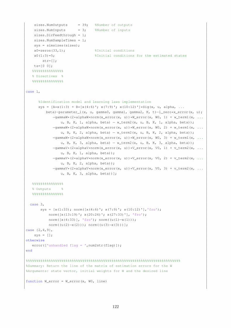
sizes.NumOutputs = 39; %Number of outputs

sizes.NumInputs = 3; %Number of inputs

sizes.DirFeedthrough = 1;

sizes.NumSampleTimes = 1;

sys = simsizes(sizes);

x0=zeros(33,1); %Initial conditions

x0(1:3)=5; %Initial conditions for the estimated states

str=[];

ts=[0 0];

%%%%%%%%%%%%%%%

% Directives %

%%%%%%%%%%%%%%%

case 1,

%Identification model and learning laws implementation

sys = [A*x(1:3) + B*[x(4:6)'; x(7:9)'; x(10:12)']*Sig(x, u, alpha, ...

beta)�parameter_l(x, u, gamma0, gamma1, gamma2, K, t)�l_zero*x_error(x, u);

�gammaW*(2*alphaW*norm(x_error(x, u))*W_error(x, W0, 1) + w_term1(x, ...

u, B, K, 1, alpha, beta) � w_term2(x, u, B, K, 1, alpha, beta));

�gammaW*(2*alphaW*norm(x_error(x, u))*W_error(x, W0, 2) + w_term1(x, ...

u, B, K, 2, alpha, beta) � w_term2(x, u, B, K, 2, alpha, beta));

�gammaW*(2*alphaW*norm(x_error(x, u))*W_error(x, W0, 3) + w_term1(x, ...

u, B, K, 3, alpha, beta) � w_term2(x, u, B, K, 3, alpha, beta));

�gammaV*(2*alphaV*norm(x_error(x, u))*V_error(x, V0, 1) + v_term2(x, ...

u, B, K, 1, alpha, beta));

�gammaV*(2*alphaV*norm(x_error(x, u))*V_error(x, V0, 2) + v_term2(x, ...

u, B, K, 2, alpha, beta));

�gammaV*(2*alphaV*norm(x_error(x, u))*V_error(x, V0, 3) + v_term2(x, ...

u, B, K, 3, alpha, beta))];

%%%%%%%%%%%%%%%

% Outputs %

%%%%%%%%%%%%%%%

case 3,

sys = [x(1:33); norm([x(4:6)'; x(7:9)'; x(10:12)'],'fro');

norm([x(13:19)'; x(20:26)'; x(27:33)'], 'fro');

norm([x(4:33)], 'fro'); norm((u(1)�x(1)));norm((u(2)�x(2))); norm((u(3)�x(3)))];

case {2,4,9},

sys = [];

otherwise

error(['unhandled flag = ',num2str(flag)]);

end

%%%%%%%%%%%%%%%%%%%%%%%%%%%%%%%%%%%%%%%%%%%%%%%%%%%%%%%%%%%%%%%%%%%%%%%%%%

%Summary: Return the line of the matrix of estimation errors for the W

%Arguments: state vector, initial weights for W and the desired line

function W_error = W_error(x, W0, line)

122

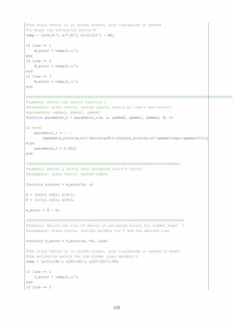
%The state vector is in column format, your transposed is needed

%to mount the estimation matrix W

temp = [x(4:6)'; x(7:9)'; x(10:12)'] � W0;

if line == 1

W_error = temp(1,:)';

end

if line == 2

W_error = temp(2,:)';

end

if line == 3

W_error = temp(3,:)';

end

%%%%%%%%%%%%%%%%%%%%%%%%%%%%%%%%%%%%%%%%%%%%%%%%%%%%%%%%%%%%%%%%%%%%%%%%%%%%%%%%%%%%%%%%%%%%%%%%%%%

%Summary: Return the vector function l

%Arguments: state vector, system inputs, matrix K, time t and control

%parameters: gamma0, gamma1, gamma2

function parameter_l = parameter_l(x, u, gamma0, gamma1, gamma2, K, t)

if t<=3

parameter_l = � ...

(gamma0*x_error(x,u))/(min(eig(K))*(norm(x_error(x,u))+gamma1*exp(�gamma2*t)));else

parameter_l = 0.001;

end

%%%%%%%%%%%%%%%%%%%%%%%%%%%%%%%%%%%%%%%%%%%%%%%%%%%%%%%%%%%%%%%%%%%%%%%%%

%Summary: Return a vector with estimated state's errors

%Arguments: state vector, system inputs

function x_error = x_error(x, u)

X = [x(1); x(2); x(3)];

U = [u(1); u(2); u(3)];

x_error = X � U;

%%%%%%%%%%%%%%%%%%%%%%%%%%%%%%%%%%%%%%%%%%%%%%%%%%%%%%%%%%%%%%%%%%%%%%%%%%%

%Summary: Return the line of matrix of estimated errors for hidden layer V

%Arguments: state vector, initial weights for V and the desired line

function V_error = V_error(x, V0, line)

%The state vector is in column format, your transposed is needed to mount

%the estimation matrix for the hidden layer weights V

temp = [x(13:19)'; x(20:26)'; x(27:33)']�V0;

if line == 1

V_error = temp(1,:)';

end

if line == 2

123

V_error = temp(2,:)';

end

if line == 3

V_error = temp(3,:)';

end

%%%%%%%%%%%%%%%%%%%%%%%%%%%%%%%%%%%%%%%%%%%%%%%%%%%%%%%%%%%%%%%%%%%%%%%%%%

%Summary: Return the NN's nonlinear regressor vector

%Arguments: state vector, system inputs and sigmoidal function parameters

function Sig = Sig(x,u, alpha, beta) %Regressor

%Parameters for the activation function

VZ = [x(13:19)'; x(20:26)'; x(27:33)']*[u(1); u(2); u(3); u(1)^2; u(2)^2; u(3)^2; 1];

%A sigmoidal function is used, we pass each of the elements of the vector

Sig=[(z(VZ(1), alpha, beta));

(z(VZ(2), alpha, beta));

(z(VZ(3), alpha, beta))];

%%%%%%%%%%%%%%%%%%%%%%%%%%%%%%%%%%%%%%%%%%%%%%%%%%%%%%%%%%%%%%%%%%%%%%%%%%

%Summary: Sigmoidal fucntion that returns the results of the regressor

%Arguments: the product VZ and parameters for the sigmoidal function

function z = z(arg, alpha, beta) %Sigmoidal activation function

z=alpha/(1+exp(�beta*arg)); %Sigmoidal Function

%%%%%%%%%%%%%%%%%%%%%%%%%%%%%%%%%%%%%%%%%%%%%%%%%%%%%%%%%%%%%%%%%%%%%%%%%%

%Summary: Return the derivative of the NN's nonlinear regressor

%Arguments: state vectors, system inputs and sigmoidal function parameters

function Sigdot = Sigdot(x,u, alpha, beta) %Regressor

%Parameters for the activation function

VZ = [x(13:19)'; x(20:26)'; x(27:33)']*[u(1); u(2); u(3); u(1)^2; u(2)^2; u(3)^2; 1];

%A sigmoidal function is used, passing each of the elements and creating a

%diagonal matrix

Sigdot=[zdot(VZ(1), alpha, beta) 0 0;

0 zdot(VZ(2), alpha, beta) 0;

0 0 zdot(VZ(3), alpha, beta)];

%%%%%%%%%%%%%%%%%%%%%%%%%%%%%%%%%%%%%%%%%%%%%%%%%%%%%%%%%%%%%%%%%%%%%%%%%%

%Summary: Derivative of the sigmoidal function that returns the regressor results

%Arguments: the product VZ, parameters for sigmoidal function

%Derivative of the sigmoidal activation function

function zdot = zdot(arg,alpha,beta)

%derivative of the sigmoidal function

zdot=(alpha*exp(�beta*arg))/(1+exp(�beta*arg)^2);

124

%%%%%%%%%%%%%%%%%%%%%%%%%%%%%%%%%%%%%%%%%%%%%%%%%%%%%%%%%%%%%%%%%%%%%%%%%%

%Summary: Return the line of B*K*Xerror*S(VZ)

%Arguments: state vector, system inputs, matrix B and K, desired line of the ...

matrix and parameters of sigmoidal function

function w_term1 = w_term1(x, u, B, K, line, alpha, beta)

%term B*K*Xerror*S(VZ) 3x3

temp = B*K*x_error(x,u)*(Sig(x,u, alpha, beta)');

if line == 1

w_term1 = temp(1, :)';

end

if line == 2

w_term1 = temp(2, :)';

end

if line == 3

w_term1 = temp(3, :)';

end

%%%%%%%%%%%%%%%%%%%%%%%%%%%%%%%%%%%%%%%%%%%%%%%%%%%%%%%%%%%%%%

%Summary: Return the line of B*K*Xerror*(Sdot(VZ)*VZ)'

%Arguments: state vector, system inputs, matrix B and K,

%desired line and parameters of sigmoidal function

function w_term2 = w_term2(x, u, B, K, line, alpha, beta)

%Parameters for the activation function

VZ = [x(13:19)'; x(20:26)'; x(27:33)']*[u(1); u(2); u(3); u(1)^2; u(2)^2; u(3)^2; 1];

%Term B*K*Xerror*(Sdot(VZ)*VZ)'

temp = B*K*x_error(x,u)*((Sigdot(x,u, alpha, beta)*VZ)');

if line == 1

w_term2 = temp(1, :)';

end

if line == 2

w_term2 = temp(2, :)';

end

if line == 3

w_term2 = temp(3, :)';

end

%%%%%%%%%%%%%%%%%%%%%%%%%%%%%%%%%%%%%%%%%%%%%%%%%%%%%%%%%%%%%%

%Summary: Return the line of Sdot(VZ)*W'*B*K*Xerror*Z'

%Arguments: state vector, system inputs, matrix B and K,

%desired line and parameters of sigmoidal function

function v_term2 = v_term2(x, u, B, K, line, alpha, beta)

%The vector of states is in column format, the following matrix is already transposed

125

W_transposed = [x(4:6) x(7:9) x(10:12)];

Z = [u(1); u(2); u(3); u(1)^2; u(2)^2; u(3)^2; 1];

%Term Sdot(VZ)*W'*B*K*Xerror*Z'

temp = Sigdot(x,u, alpha, beta)'*W_transposed*B*K*x_error(x,u)*(Z');

if line == 1

v_term2 = temp(1, :)';

end

if line == 2

v_term2 = temp(2, :)';

end

if line == 3

v_term2 = temp(3, :)';

end

I.18 Appendix 18 - Code to display the Fig. 5.1-5.5

%Displays the actual states and their estimations

fsize=22;

figure;

plot(t,x(:,1),'��',t,Xestimated(:,1),'LineWidth',2);set(0,'DefaultAxesFontSize', 17);

h=legend('Actual','Estimated');

set(h,'FontSize',fsize);

xlabel('Time(s)','interpreter','latex','Fontsize',fsize);

ylabel('x_{1}(t), x_{NN1}(t)','Fontsize',fsize);

figure;

plot(t,x(:,2),'��',t,Xestimated(:,2),'LineWidth',2);set(0,'DefaultAxesFontSize', 17);

h=legend('Actual','Estimated');

set(h,'FontSize',fsize);

xlabel('Time(s)','interpreter','latex','Fontsize',fsize);

ylabel('x_{2}(t), x_{NN2}(t)','Fontsize',fsize);

figure;

plot(t,x(:,3),'��',t,Xestimated(:,3),'LineWidth',2);set(0,'DefaultAxesFontSize', 17);

h=legend('Actual','Estimated');

set(h,'FontSize',fsize);

xlabel('Time(s)','interpreter','latex','Fontsize',fsize);

ylabel('x_{3}(t), x_{NN3}(t)','Fontsize',fsize);

figure;

plot(t, Xestimated(:,34), 'LineWidth', 2 );

set(0,'DefaultAxesFontSize', 17);

126

set(h,'FontSize',fsize);

xlabel('Time(s)','interpreter','latex','Fontsize',fsize);

ylabel('Estimated weight matrix W','Fontsize',fsize);

figure;

plot(t, Xestimated(:,35), 'LineWidth', 2 );

set(0,'DefaultAxesFontSize', 17);

set(h,'FontSize',fsize);

xlabel('Time(s)','interpreter','latex','Fontsize',fsize);

ylabel('Estimated weight matrix V','Fontsize',fsize);

I.19 Appendix 19 - Code for plant model corresponding to Fig.5.6-5.10

function [sys,x0,str,ts] = Plant(t,x,u,flag)

% Unified chaotic system

a=1; %Constant for chen system

switch flag,

%%%%%%%%%%%%%%%%%%

% Initialization %

%%%%%%%%%%%%%%%%%%

case 0,

sizes = simsizes;

sizes.NumContStates = 3; %Number of Constant States

sizes.NumDiscStates = 0; %Number of Discret States

sizes.NumOutputs = 3; %Number of Outputs

sizes.NumInputs = 0; %Number of Inputs

sizes.DirFeedthrough = 1;

sizes.NumSampleTimes = 1;

sys = simsizes(sizes);

x0=[2 1 2]; %Initial Conditions

str=[];

ts=[0 0];

%%%%%%%%%%%%%%%

% Directives %

%%%%%%%%%%%%%%%

case 1,

%Implementation of Unified Chaotic System, the constant value generates

%a Chen System.

sys(1) = (25*a+10)*(x(2)�x(1));sys(2) = (28�35*a)*x(1)�x(1)*x(3)+(29*a�1)*x(2)+disturb(x,u,t);sys(3) = x(1)*x(2)�((a+8)/3)*x(3)+disturb(x,u,t);%%%%%%%%%%

% Outputs %

127

%%%%%%%%%%

case 3,

sys = x;

%%%%%%%%%%%%%

% End %

%%%%%%%%%%%%%

case {2,4,9},

sys = [];

otherwise

error(['unhandled flag = ',num2str(flag)]);

end

%%%%%%%%%%%%%%%%%%%%%%%%%%%%%%%%%%%%%%%%%%%%%%%%%%%%%%%%%%%%%%

%Summary: Return the system's perturbations

%Arguments: state vector, input vector and time

function disturb = disturb(x,u,t)

if t>=5

disturb=3*sin(t)*(sqrt(x(1)^2 + x(2)^2 + x(3)^2))+50*sin(200*t)+10*cos(400*t);

else

disturb=0; %Until t=5 secs the disturb is null

end

I.20 Appendix 20 - Code for identifier corresponding to Fig. 5.6-5.10

%Project description: Online Identification using hidden layer neural

% networks with adaptive laws under disturbances

%Authors: Jose Alfredo Ruiz Vargas and Emerson Grzeidak

%Date: 04/2015 Local: University of Brasilia

function [sys,x0,str,ts] = iden_Caos(t,x,u,flag)

%Diagonal matrix A with negative elements

A = [�7.8 0 0; 0 �7.8 0; 0 0 �7.8];

%Diagonal matrix A with positive elements

B = 110*[1.1 0 0; 0 1.16 0; 0 0 1.3];

%Positive constants for fine tunning of the neural network

gammaW=0.02;

gammaV=0.001;

gamma0 = 0.1;

gamma1 = 1;

gamma2 = 1;

alphaW=0.5;

128

alphaV=0.5;

l_zero = 1;

%Adjustment weights to the output layer

W0 = [0 0 0; 0 0 0; 0 0 0];

%Adjustment weights to the hidden layer

V0 = [0 0 0 0 0 0 0; 0 0 0 0 0 0 0; 0 0 0 0 0 0 0];

%Positive definite matrix P

P = 50*[0.001 0 0; 0 0.001 0; 0 0 0.001];

%Matrix K

K = P + P';

%Numerator parameter for the sigmoidal function

alpha=85;

%Denominator parameter for the sigmoidal function

beta=1;

switch flag,

%%%%%%%%%%%%%%%%%%

% Initialization %

%%%%%%%%%%%%%%%%%%

case 0,

sizes = simsizes;

sizes.NumContStates = 33; %Number of continuous states

sizes.NumDiscStates = 0; %Number of discrete states

sizes.NumOutputs = 39; %Number of outputs

sizes.NumInputs = 3; %Number of inputs

sizes.DirFeedthrough = 1;

sizes.NumSampleTimes = 1;

sys = simsizes(sizes);

x0=zeros(33,1); %Initial conditions

x0(1:3)=5;

%Initial conditions for the estimated states

str=[];

ts=[0 0];

%%%%%%%%%%%%%%%

% Directives %

%%%%%%%%%%%%%%%

case 1,

%Identification Model and Learning Laws implementation

sys = [A*x(1:3) + B*[x(4:6)'; x(7:9)'; x(10:12)']*Sig(x, u, alpha, ...

beta)�parameter_l(x, u, gamma0, gamma1, gamma2, K, t)�l_zero*x_error(x, u);

129

�gammaW*(2*alphaW*norm(x_error(x, u))*W_error(x, W0, 1) + w_term1(x, ...

u, B, K, 1, alpha, beta) � w_term2(x, u, B, K, 1, alpha, beta));

�gammaW*(2*alphaW*norm(x_error(x, u))*W_error(x, W0, 2) + w_term1(x, ...

u, B, K, 2, alpha, beta) � w_term2(x, u, B, K, 2, alpha, beta));

�gammaW*(2*alphaW*norm(x_error(x, u))*W_error(x, W0, 3) + w_term1(x, ...

u, B, K, 3, alpha, beta) � w_term2(x, u, B, K, 3, alpha, beta));

�gammaV*(2*alphaV*norm(x_error(x, u))*V_error(x, V0, 1) + v_term2(x, ...

u, B, K, 1, alpha, beta));

�gammaV*(2*alphaV*norm(x_error(x, u))*V_error(x, V0, 2) + v_term2(x, ...

u, B, K, 2, alpha, beta));

�gammaV*(2*alphaV*norm(x_error(x, u))*V_error(x, V0, 3) + v_term2(x, ...

u, B, K, 3, alpha, beta))];

%%%%%%%%%%%%%%%

% Outputs %

%%%%%%%%%%%%%%%

case 3,

sys = [x(1:33); norm([x(4:6)'; x(7:9)'; x(10:12)'],'fro'); ...

norm([x(13:19)'; x(20:26)'; x(27:33)'], 'fro'); norm([x(4:33)], 'fro'); ...

norm((u(1)�x(1))); norm((u(2)�x(2))); norm((u(3)�x(3)))];case {2,4,9},

sys = [];

otherwise

error(['unhandled flag = ',num2str(flag)]);

end

%%%%%%%%%%%%%%%%%%%%%%%%%%%%%%%%%%%%%%%%%%%%%%%%%%%%%%%%%%%%%%

%Summary: Return the line of the matrix of estimation errors for the parameter W

%Arguments: state vector, initial weights for W and the desired line

function W_error = W_error(x, W0, line)

%The state vector is in column format, your transposed is needed

%to mount the estimation matrix W

temp = [x(4:6)'; x(7:9)'; x(10:12)'] � W0;

if line == 1

W_error = temp(1,:)';

end

if line == 2

W_error = temp(2,:)';

end

if line == 3

W_error = temp(3,:)';

end

%%%%%%%%%%%%%%%%%%%%%%%%%%%%%%%%%%%%%%%%%%%%%%%%%%%%%%%%%%%%%%%%%%%%%%%%%%%%%%%%%%%%%%%%%%%%%%%%%%%

%Summary: Return the vector function l

%Arguments: state vector, system inputs, matrix K, time t and control

%parameters: gamma0, gamma1, gamma2

function parameter_l = parameter_l(x, u, gamma0, gamma1, gamma2, K, t)

130

if t<=3

parameter_l = � ...

(gamma0*x_error(x,u))/(min(eig(K))*(norm(x_error(x,u))+gamma1*exp(�gamma2*t)));else

parameter_l = 0.001;

end

%%%%%%%%%%%%%%%%%%%%%%%%%%%%%%%%%%%%%%%%%%%%%%%%%%%%%%%%%%%%%%

%Summary: Return a vector with estimated state's errors

%Arguments: state vector, system inputs

function x_error = x_error(x, u)

X = [x(1); x(2); x(3)];

U = [u(1); u(2); u(3)];

x_error = X � U;

%%%%%%%%%%%%%%%%%%%%%%%%%%%%%%%%%%%%%%%%%%%%%%%%%%%%%%%%%%%%%%

%Summary: Return the line of the matrix of estimated errors for hidden layer ...

weights V

%Arguments: state vector, initial weights for hidden layer V and the desired line

function V_error = V_error(x, V0, line)

%The state vector is in column format, your transposed is needed to mount

%the estimation matrix for the hidden layer weights V

temp = [x(13:19)'; x(20:26)'; x(27:33)']�V0;

if line == 1

V_error = temp(1,:)';

end

if line == 2

V_error = temp(2,:)';

end

if line == 3

V_error = temp(3,:)';

end

%%%%%%%%%%%%%%%%%%%%%%%%%%%%%%%%%%%%%%%%%%%%%%%%%%%%%%%%%%%%%%

%Summary: Return the NN's nonlinear regressor vector

%Arguments: state vector, system inputs and sigmoidal function parameters

function Sig = Sig(x,u, alpha, beta) %Regressor

%Parameters for the activation function

VZ = [x(13:19)'; x(20:26)'; x(27:33)']*[u(1); u(2); u(3); u(1)^2; u(2)^2; u(3)^2; 1];

%A sigmoidal function is used, we pass each of the elements of the vector

Sig=[(z(VZ(1), alpha, beta));

(z(VZ(2), alpha, beta));

131

(z(VZ(3), alpha, beta))];

%%%%%%%%%%%%%%%%%%%%%%%%%%%%%%%%%%%%%%%%%%%%%%%%%%%%%%%%%%%%%%

%Summary: Sigmoidal fucntion that returns the results of the regressor

%Arguments: the product VZ and parameters for the sigmoidal function

function z = z(arg, alpha, beta) %Sigmoidal activation function

z=alpha/(1+exp(�beta*arg)); %Sigmoidal Function

%%%%%%%%%%%%%%%%%%%%%%%%%%%%%%%%%%%%%%%%%%%%%%%%%%%%%%%%%%%%%%

%Summary: Return the derivative of the NN's nonlinear regressor

%Arguments: state vectors, system inputs and sigmoidal function parameters

function Sigdot = Sigdot(x,u, alpha, beta) %Regressor

%Parameters for the activation function

VZ = [x(13:19)'; x(20:26)'; x(27:33)']*[u(1); u(2); u(3); u(1)^2; u(2)^2; u(3)^2; 1];

%A sigmoidal function is used, passing each of the elements and creating a

%diagonal matrix

Sigdot=[zdot(VZ(1), alpha, beta) 0 0;

0 zdot(VZ(2), alpha, beta) 0;

0 0 zdot(VZ(3), alpha, beta)];

%%%%%%%%%%%%%%%%%%%%%%%%%%%%%%%%%%%%%%%%%%%%%%%%%%%%%%%%%%%%%%

%Summary: Derivative of the sigmoidal function that returns the regressor results

%Arguments: the product VZ, parameters for sigmoidal function

%Derivative of the sigmoidal activation function

function zdot = zdot(arg,alpha,beta)

%derivative of the sigmoidal function

zdot=(alpha*exp(�beta*arg))/(1+exp(�beta*arg)^2);

%%%%%%%%%%%%%%%%%%%%%%%%%%%%%%%%%%%%%%%%%%%%%%%%%%%%%%%%%%%%%%

%Summary: Return the line of B*K*Xerro*S(VZ)

%Arguments: state vector, system inputs, matrix B and K,

%desired line of the matrix and parameters of sigmoidal function

function w_term1 = w_term1(x, u, B, K, line, alpha, beta)

%term B*K*Xerror*S(VZ) 3x3

temp = B*K*x_error(x,u)*(Sig(x,u, alpha, beta)');

if line == 1

w_term1 = temp(1, :)';

end

if line == 2

w_term1 = temp(2, :)';

end

if line == 3

132

w_term1 = temp(3, :)';

end

%%%%%%%%%%%%%%%%%%%%%%%%%%%%%%%%%%%%%%%%%%%%%%%%%%%%%%%%%%%%%%

%Summary: Return the line of B*K*Xerror*(Sdot(VZ)*VZ)'

%Arguments: state vector, system inputs, matrix B and K,

%desired line and parameters of sigmoidal function

function w_term2 = w_term2(x, u, B, K, line, alpha, beta)

%Parameters for the activation function

VZ = [x(13:19)'; x(20:26)'; x(27:33)']*[u(1); u(2); u(3); u(1)^2; u(2)^2; u(3)^2; 1];

%Term B*K*Xerror*(Sdot(VZ)*VZ)'

temp = B*K*x_error(x,u)*((Sigdot(x,u, alpha, beta)*VZ)');

if line == 1

w_term2 = temp(1, :)';

end

if line == 2

w_term2 = temp(2, :)';

end

if line == 3

w_term2 = temp(3, :)';

end

%%%%%%%%%%%%%%%%%%%%%%%%%%%%%%%%%%%%%%%%%%%%%%%%%%%%%%%%%%%%%%

%Summary: Return the line of Sdot(VZ)*W'*B*K*Xerror*Z'

%Arguments: state vector, system inputs, matrix B and K,

%desired line and parameters of sigmoidal function

function v_term2 = v_term2(x, u, B, K, line, alpha, beta)

%The vector of states is in column format, the following matrix is already transposed

W_transposed = [x(4:6) x(7:9) x(10:12)];

Z = [u(1); u(2); u(3); u(1)^2; u(2)^2; u(3)^2; 1];

%Term Sdot(VZ)*W'*B*K*Xerror*Z'

temp = Sigdot(x,u, alpha, beta)'*W_transposed*B*K*x_error(x,u)*(Z');

if line == 1

v_term2 = temp(1, :)';

end

if line == 2

v_term2 = temp(2, :)';

end

if line == 3

v_term2 = temp(3, :)';

end

133

I.21 Appendix 21 - Code to display the Fig. 5.6-5.10

%Displays the actual states and their estimations

fsize=22;

figure;

plot(t,x(:,1),'��',t,Xestimated(:,1),'LineWidth',2);set(0,'DefaultAxesFontSize', 17);

h=legend('Actual','Estimated');

set(h,'FontSize',fsize);

xlabel('Time(s)','interpreter','latex','Fontsize',fsize);

ylabel('x_{1}(t), x_{NN1}(t)','Fontsize',fsize);

figure;

plot(t,x(:,2),'��',t,Xestimated(:,2),'LineWidth',2);set(0,'DefaultAxesFontSize', 17);

h=legend('Actual','Estimated');

set(h,'FontSize',fsize);

xlabel('Time(s)','interpreter','latex','Fontsize',fsize);

ylabel('x_{2}(t), x_{NN2}(t)','Fontsize',fsize);

figure;

plot(t,x(:,3),'��',t, Xestimated(:,3),'LineWidth',2);

set(0,'DefaultAxesFontSize', 17);

h=legend('Actual','Estimated');

set(h,'FontSize',fsize);

xlabel('Time(s)','interpreter','latex','Fontsize',fsize);

ylabel('x_{3}(t), x_{NN3}(t)','Fontsize',fsize);

figure;

plot(t,Xestimated(:,34),'LineWidth',2);

set(0,'DefaultAxesFontSize', 17);

set(h,'FontSize',fsize);

xlabel('Time(s)','interpreter','latex','Fontsize',fsize);

ylabel('Estimated weight matrix W','Fontsize',fsize);

figure;

plot(t,Xestimated(:,35),'LineWidth',2);

set(0,'DefaultAxesFontSize', 17);

set(h,'FontSize',fsize);

xlabel('Time(s)','interpreter','latex','Fontsize',fsize);

ylabel('Estimated weight matrix V','Fontsize',fsize);

I.22 Appendix 22 - Code for plant model corresponding to Fig.5.11-5.19

134

function [sys,x0,str,ts] = plant(t,x,u,flag)

% Hyperchaotic Complex System

%System's parameters constants

alpha=14;

beta=3;

gamma=50;

k1=�5;k2=�4;

switch flag,

%%%%%%%%%%%%%%%%%%

% Initialization %

%%%%%%%%%%%%%%%%%%

case 0,

sizes = simsizes;

sizes.NumContStates = 7; %Number of Continuous States

sizes.NumDiscStates = 0; %Number of Discret States

sizes.NumOutputs = 7; %Number of Outputs

sizes.NumInputs = 0; %Number of Inputs

sizes.DirFeedthrough = 1;

sizes.NumSampleTimes = 1;

sys = simsizes(sizes);

x0=[0 1 2 3 4 5 6]; %Initial Conditions

str=[];

ts=[0 0];

%%%%%%%%%%%%%%%

% Directives %

%%%%%%%%%%%%%%%

case 1,

%Hyperchaotic Complex System equations

sys = [alpha*(x(3)�x(1));alpha*(x(4)�x(2));gamma*x(1)�x(1)*x(5)�x(3)+x(6);gamma*x(2)�x(2)*x(5)�x(4)+x(7);x(1)*x(3)+x(2)*x(4)�beta*x(5);k1*x(1)+k2*x(3);

k1*x(2)+k2*x(4)]+disturb(x,u,t);

%%%%%%%%%%

% Output %

%%%%%%%%%%

case 3,

sys = x;

%%%%%%%%%%%%%

% END %

%%%%%%%%%%%%%

case {2,4,9},

sys = [];

otherwise

error(['unhandled flag = ',num2str(flag)]);

135

end

%%%%%%%%%%%%%%%%%%%%%%%%%%%%%%%%%%%%%%%%%%%%%%%%%%%%%%%%%%%%%%

%Summary: Return the system's perturbations

%Arguments: state vector, input vector and time

function disturb = disturb(x,u,t)

if t>=5

n=sqrt(x(1)^2 + x(2)^2 + x(3)^2+x(4)^2+x(5)^2 + x(6)^2 + x(7)^2);

disturb=1.8*[n*sin(t);

n*1.2*sin(2*t);

n*cos(4*t);

n*1.2*sin(t);

n*1.1*sin(2*t) ;

n*0.5*sin(4*t);

exp(�0.5*t)];else

disturb=[0 ; 0; 0; 0; 0; 0; 0]; %Before t=5s, the disturbance is null

end

I.23 Appendix 23 - Code for identifier corresponding to Fig. 5.11-5.19

%Project description: Online Identification using hidden layer neural networks

% with adaptive laws

%Authors: Jose Alfredo Ruiz Vargas and Emerson Grzeidak

%Date: 04/2016 Local: University of Brasilia

function [sys,x0,str,ts] = iden_Caos(t,x,u,flag)

%Diagonal matrix A with negative elements

A = 10*[�2 0 0 0 0 0 0;

0 �2 0 0 0 0 0;

0 0 �2 0 0 0 0;

0 0 0 �2 0 0 0;

0 0 0 0 �2 0 0;

0 0 0 0 0 �2 0;

0 0 0 0 0 0 �2];

%Diagonal matrix A with positive elements

B = 100*[1 0 0 0 0 0 0;

0 1 0 0 0 0 0;

0 0 1 0 0 0 0;

0 0 0 1 0 0 0;

0 0 0 0 1 0 0;

0 0 0 0 0 1 0;

0 0 0 0 0 0 1];

136

% Parameters for the identification model and adaptive laws

gammaW=0.001;

gammaV=1;

gamma0 = 0.1;

gamma1 = 1;

gamma2 = 1;

alphaW=0.5;

alphaV=0.5;

l0 = 10;

%Adjustment weights to the output layer

W0 = [0 0 0 0 0 0 0;

0 0 0 0 0 0 0;

0 0 0 0 0 0 0;

0 0 0 0 0 0 0;

0 0 0 0 0 0 0;

0 0 0 0 0 0 0;

0 0 0 0 0 0 0];

%Adjustment weights to the hidden layer

V0 = [0 0 0 0 0 0 0 0;

0 0 0 0 0 0 0 0;

0 0 0 0 0 0 0 0;

0 0 0 0 0 0 0 0;

0 0 0 0 0 0 0 0;

0 0 0 0 0 0 0 0;

0 0 0 0 0 0 0 0];

%Positive definite matrix P

P = 0.05*[1 0 0 0 0 0 0;

0 1 0 0 0 0 0;

0 0 1 0 0 0 0;

0 0 0 1 0 0 0;

0 0 0 0 1 0 0;

0 0 0 0 0 1 0;

0 0 0 0 0 0 1];

%Matrix K

K = P + P';

%Numerator parameter for the sigmoidal function

alpha=150;

%Denominator parameter for the sigmoidal function

beta=1;

switch flag,

%%%%%%%%%%%%%%%%%%

137

% Initialization %

%%%%%%%%%%%%%%%%%%

case 0,

sizes = simsizes;

sizes.NumContStates = 112; %Number of continuous states

sizes.NumDiscStates = 0; %Number of discrete states

sizes.NumOutputs = 9; %Number of outputs

sizes.NumInputs = 7; %Number of inputs

sizes.DirFeedthrough = 1;

sizes.NumSampleTimes = 1;

sys = simsizes(sizes);

x0=zeros(112,1); %Initial conditions

x0(1:7)=[�50 �30 �40 20 40 50 40]; %Initial conditions for the estimated states

str=[];

ts=[0 0];

%%%%%%%%%%%%%%%

% Directives %

%%%%%%%%%%%%%%%

case 1,

%Identification Model and Learning Laws implementation

sys = [A*x(1:7) + B*[x(8:14)'; x(15:21)'; x(22:28)'; x(29:35)'; x(36:42)'; ...

x(43:49)'; x(50:56)']*Sig(x, u, alpha, beta)�parameter_l(x, u, gamma0, ...

gamma1, gamma2, K, t)�l0*x_error(x,u);�gammaW*(2*alphaW*norm(x_error(x, u))*W_error(x, W0, 1) + w_term1(x, ...

u, B, K, 1, alpha, beta) � w_term2(x, u, B, K, 1, alpha, beta));

�gammaW*(2*alphaW*norm(x_error(x, u))*W_error(x, W0, 2) + w_term1(x, ...

u, B, K, 2, alpha, beta) � w_term2(x, u, B, K, 2, alpha, beta));

�gammaW*(2*alphaW*norm(x_error(x, u))*W_error(x, W0, 3) + w_term1(x, ...

u, B, K, 3, alpha, beta) � w_term2(x, u, B, K, 3, alpha, beta));

�gammaW*(2*alphaW*norm(x_error(x, u))*W_error(x, W0, 4) + w_term1(x, ...

u, B, K, 4, alpha, beta) � w_term2(x, u, B, K, 4, alpha, beta));

�gammaW*(2*alphaW*norm(x_error(x, u))*W_error(x, W0, 5) + w_term1(x, ...

u, B, K, 5, alpha, beta) � w_term2(x, u, B, K, 5, alpha, beta));

�gammaW*(2*alphaW*norm(x_error(x, u))*W_error(x, W0, 6) + w_term1(x, ...

u, B, K, 6, alpha, beta) � w_term2(x, u, B, K, 6, alpha, beta));

�gammaW*(2*alphaW*norm(x_error(x, u))*W_error(x, W0, 7) + w_term1(x, ...

u, B, K, 7, alpha, beta) � w_term2(x, u, B, K, 7, alpha, beta));

�gammaV*(2*alphaV*norm(x_error(x, u))*V_error(x, V0, 1) + v_term2(x, ...

u, B, K, 1, alpha, beta));

�gammaV*(2*alphaV*norm(x_error(x, u))*V_error(x, V0, 2) + v_term2(x, ...

u, B, K, 2, alpha, beta));

�gammaV*(2*alphaV*norm(x_error(x, u))*V_error(x, V0, 3) + v_term2(x, ...

u, B, K, 3, alpha, beta));

�gammaV*(2*alphaV*norm(x_error(x, u))*V_error(x, V0, 4) + v_term2(x, ...

u, B, K, 4, alpha, beta));

�gammaV*(2*alphaV*norm(x_error(x, u))*V_error(x, V0, 5) + v_term2(x, ...

u, B, K, 5, alpha, beta));

138

�gammaV*(2*alphaV*norm(x_error(x, u))*V_error(x, V0, 6) + v_term2(x, ...

u, B, K, 6, alpha, beta));

�gammaV*(2*alphaV*norm(x_error(x, u))*V_error(x, V0, 7) + v_term2(x, ...

u, B, K, 7, alpha, beta))];

%%%%%%%%%%%%%%%

% Outputs %

%%%%%%%%%%%%%%%

case 3,

sys = [x(1:7);

norm([x(8:14)'; x(15:21)'; x(22:28)'; x(29:35)'; x(36:42)'; ...

x(43:49)'; x(50:56)'],'fro');

norm([x(57:64)'; x(65:72)'; x(73:80)'; x(81:88)'; x(89:96)'; ...

x(97:104)'; x(105:112)'],'fro')];

case {2,4,9},

sys = [];

otherwise

error(['unhandled flag = ',num2str(flag)]);

end

%%%%%%%%%%%%%%%%%%%%%%%%%%%%%%%%%%%%%%%%%%%%%%%%%%%%%%%%%%%%%%

%Summary: Return the line of the matrix of estimation errors for the parameter W

%Arguments: state vector, initial weights for W and the desired line

function W_error = W_error(x, W0, line)

%The state vector is in column format, your transposed is needed

%to mount the estimation matrix W

temp = [x(8:14)'; x(15:21)'; x(22:28)'; x(29:35)'; x(36:42)'; x(43:49)'; ...

x(50:56)'] � W0;

if line == 1

W_error = temp(1,:)';

end

if line == 2

W_error = temp(2,:)';

end

if line == 3

W_error = temp(3,:)';

end

if line == 4

W_error = temp(4,:)';

end

if line == 5

W_error = temp(5,:)';

end

if line == 6

W_error = temp(6,:)';

end

if line == 7

W_error = temp(7,:)';

139

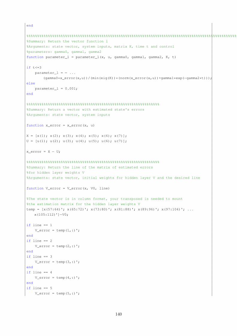
end

%%%%%%%%%%%%%%%%%%%%%%%%%%%%%%%%%%%%%%%%%%%%%%%%%%%%%%%%%%%%%%%%%%%%%%%%%%%%%%%%%%%%%%%%%%%%%%%%%%%

%Summary: Return the vector function l

%Arguments: state vector, system inputs, matrix K, time t and control

%parameters: gamma0, gamma1, gamma2

function parameter_l = parameter_l(x, u, gamma0, gamma1, gamma2, K, t)

if t<=3

parameter_l = � ...

(gamma0*x_error(x,u))/(min(eig(K))*(norm(x_error(x,u))+gamma1*exp(�gamma2*t)));else

parameter_l = 0.001;

end

%%%%%%%%%%%%%%%%%%%%%%%%%%%%%%%%%%%%%%%%%%%%%%%%%%%%%%%%%%%%%%

%Summary: Return a vector with estimated state's errors

%Arguments: state vector, system inputs

function x_error = x_error(x, u)

X = [x(1); x(2); x(3); x(4); x(5); x(6); x(7)];

U = [u(1); u(2); u(3); u(4); u(5); u(6); u(7)];

x_error = X � U;

%%%%%%%%%%%%%%%%%%%%%%%%%%%%%%%%%%%%%%%%%%%%%%%%%%%%%%%%%%%%%%

%Summary: Return the line of the matrix of estimated errors

%for hidden layer weights V

%Arguments: state vector, initial weights for hidden layer V and the desired line

function V_error = V_error(x, V0, line)

%The state vector is in column format, your transposed is needed to mount

%the estimation matrix for the hidden layer weights V

temp = [x(57:64)'; x(65:72)'; x(73:80)'; x(81:88)'; x(89:96)'; x(97:104)'; ...

x(105:112)']�V0;

if line == 1

V_error = temp(1,:)';

end

if line == 2

V_error = temp(2,:)';

end

if line == 3

V_error = temp(3,:)';

end

if line == 4

V_error = temp(4,:)';

end

if line == 5

V_error = temp(5,:)';

140

end

if line == 6

V_error = temp(6,:)';

end

if line == 7

V_error = temp(7,:)';

end

%%%%%%%%%%%%%%%%%%%%%%%%%%%%%%%%%%%%%%%%%%%%%%%%%%%%%%%%%%%%%%

%Summary: Return the NN's nonlinear regressor vector

%Arguments: state vector, system inputs and sigmoidal function parameters

function Sig = Sig(x,u, alpha, beta) %Regressor

%Parameters for the activation function

VZ = [x(57:64)'; x(65:72)'; x(73:80)'; x(81:88)'; x(89:96)'; x(97:104)'; ...

x(105:112)' ]*[u(1); u(2); u(3); u(4); u(5); u(6); u(7); 1];

%A sigmoidal function is used, we pass each of the elements of the vector

Sig=[(z(VZ(1), alpha, beta));

(z(VZ(2), alpha, beta));

(z(VZ(3), alpha, beta));

(z(VZ(4), alpha, beta));

(z(VZ(5), alpha, beta));

(z(VZ(6), alpha, beta));

(z(VZ(7), alpha, beta))];

%%%%%%%%%%%%%%%%%%%%%%%%%%%%%%%%%%%%%%%%%%%%%%%%%%%%%%%%%%%%%%

%Summary: Sigmoidal fucntion that returns the results of the regressor

%Arguments: the product VZ and parameters for the sigmoidal function

function z = z(arg, alpha, beta) %Sigmoidal activation function

z=alpha/(1+exp(�beta*arg)); %Sigmoidal Function

%%%%%%%%%%%%%%%%%%%%%%%%%%%%%%%%%%%%%%%%%%%%%%%%%%%%%%%%%%%%%%

%Summary: Return the derivative of the NN's nonlinear regressor

%Arguments: state vectors, system inputs and sigmoidal function parameters

function Sigdot = Sigdot(x,u, alpha, beta) %Regressor

%Parameters for the activation function

VZ = [x(57:64)'; x(65:72)'; x(73:80)'; x(81:88)'; x(89:96)'; x(97:104)'; ...

x(105:112)']*[u(1); u(2); u(3); u(4); u(5); u(6); u(7); 1];

%A sigmoidal function is used, passing each of the elements and creating a

%diagonal matrix

Sigdot=[zdot(VZ(1), alpha, beta) 0 0 0 0 0 0;

0 zdot(VZ(2), alpha, beta) 0 0 0 0 0;

0 0 zdot(VZ(3), alpha, beta) 0 0 0 0;

0 0 0 zdot(VZ(4), alpha, beta) 0 0 0;

0 0 0 0 zdot(VZ(5), alpha, beta) 0 0;

141

0 0 0 0 0 zdot(VZ(6), alpha, beta) 0;

0 0 0 0 0 0 zdot(VZ(7), alpha, beta)];

%%%%%%%%%%%%%%%%%%%%%%%%%%%%%%%%%%%%%%%%%%%%%%%%%%%%%%%%%%%%%%

%Summary: Derivative of the sigmoidal function that returns the regressor results

%Arguments: the product VZ, parameters for sigmoidal function

%Derivative of the sigmoidal activation function

function zdot = zdot(arg,alpha,beta)

%derivative of the sigmoidal function

zdot=(alpha*exp(�beta*arg))/(1+exp(�beta*arg)^2);

%%%%%%%%%%%%%%%%%%%%%%%%%%%%%%%%%%%%%%%%%%%%%%%%%%%%%%%%%%%%%%

%Summary: Return the line of B*K*Xerror*S(VZ)

%Arguments: state vector, system inputs, matrix B and K,

%desired line of the matrix and parameters of sigmoidal function

function w_term1 = w_term1(x, u, B, K, line, alpha, beta)

%term B*K*Xerror*S(VZ) 3x3

temp = B*K*x_error(x,u)*(Sig(x,u, alpha, beta)');

if line == 1

w_term1 = temp(1, :)';

end

if line == 2

w_term1 = temp(2, :)';

end

if line == 3

w_term1 = temp(3, :)';

end

if line == 4

w_term1 = temp(4, :)';

end

if line == 5

w_term1 = temp(5, :)';

end

if line == 6

w_term1 = temp(6, :)';

end

if line == 7

w_term1 = temp(7, :)';

end

%%%%%%%%%%%%%%%%%%%%%%%%%%%%%%%%%%%%%%%%%%%%%%%%%%%%%%%%%%%%%%

%Summary: Return the line of B*K*Xerror*(Sdot(VZ)*VZ)'

%Arguments: state vector, system inputs, matrix B and K, %desired line and ...

parameters of sigmoidal function

function w_term2 = w_term2(x, u, B, K, line, alpha, beta)

142

%Parameters for the activation function

VZ = [x(57:64)'; x(65:72)'; x(73:80)'; x(81:88)'; x(89:96)'; x(97:104)'; ...

x(105:112)' ]*[u(1); u(2); u(3); u(4); u(5); u(6); u(7); 1];

%Term B*K*Xerror*(Sdot(VZ)*VZ)'

temp = B*K*x_error(x,u)*((Sigdot(x,u, alpha, beta)*VZ)');

if line == 1

w_term2 = temp(1, :)';

end

if line == 2

w_term2 = temp(2, :)';

end

if line == 3

w_term2 = temp(3, :)';

end

if line == 4

w_term2 = temp(4, :)';

end

if line == 5

w_term2 = temp(5, :)';

end

if line == 6

w_term2 = temp(6, :)';

end

if line == 7

w_term2 = temp(7, :)';

end

%%%%%%%%%%%%%%%%%%%%%%%%%%%%%%%%%%%%%%%%%%%%%%%%%%%%%%%%%%%%%%

%Summary: Return the line of Sdot(VZ)*W'*B*K*Xerror*Z'

%Arguments: state vector, system inputs, matrix B and K,

%desired line and parameters of sigmoidal function

function v_term2 = v_term2(x, u, B, K, line, alpha, beta)

%The vector of states is in column format, the following matrix is already transposed

W_transposed = [x(8:14) x(15:21) x(22:28) x(29:35) x(36:42) x(43:49) x(50:56)];

Z = [u(1); u(2); u(3); u(4); u(5); u(6); u(7); 1];

%Term Sdot(VZ)*W'*B*K*Xerror*Z'

temp = Sigdot(x,u, alpha, beta)'*W_transposed*B*K*x_error(x,u)*(Z');

if line == 1

v_term2 = temp(1, :)';

end

if line == 2

v_term2 = temp(2, :)';

end

if line == 3

v_term2 = temp(3, :)';

143

end

if line == 4

v_term2 = temp(4, :)';

end

if line == 5

v_term2 = temp(5, :)';

end

if line == 6

v_term2 = temp(6, :)';

end

if line == 7

v_term2 = temp(7, :)';

end

I.24 Appendix 24 - Code to display the Fig. 5.11-5.19

%Displays the actual states and their estimations

fsize=22;

figure;

plot(t, x(:,1), '��',t, Xestimated(:,1), 'LineWidth', 2 );

set(0,'DefaultAxesFontSize', 17);

h=legend('Actual','Estimated');

set(h,'FontSize',fsize);

xlabel('Time(s)','interpreter','latex','Fontsize',fsize);

ylabel('x_{1}(t), x_{NN1}(t)','Fontsize',fsize);

figure;

plot(t, x(:,2), '��',t, Xestimated(:,2), 'LineWidth', 2 );

set(0,'DefaultAxesFontSize', 17);

h=legend('Actual','Estimated');

set(h,'FontSize',fsize);

xlabel('Time(s)','interpreter','latex','Fontsize',fsize);

ylabel('x_{2}(t), x_{NN2}(t)','Fontsize',fsize);

figure;

plot(t, x(:,3), '��',t, Xestimated(:,3), 'LineWidth', 2 );

set(0,'DefaultAxesFontSize', 17);

h=legend('Actual','Estimated');

set(h,'FontSize',fsize);

xlabel('Time(s)','interpreter','latex','Fontsize',fsize);

ylabel('x_{3}(t), x_{NN3}(t)','Fontsize',fsize);

figure;

plot(t, x(:,4), '��',t, Xestimated(:,4), 'LineWidth', 2 );

set(0,'DefaultAxesFontSize', 17);

h=legend('Actual','Estimated');

set(h,'FontSize',fsize);

xlabel('Time(s)','interpreter','latex','Fontsize',fsize);

144

ylabel('x_{4}(t), x_{NN4}(t)','Fontsize',fsize);

figure;

plot(t, x(:,5), '��',t, Xestimated(:,5), 'LineWidth', 2 );

set(0,'DefaultAxesFontSize', 17);

h=legend('Actual','Estimated');

set(h,'FontSize',fsize);

xlabel('Time(s)','interpreter','latex','Fontsize',fsize);

ylabel('x_{5}(t), x_{NN5}(t)','Fontsize',fsize);

figure;

plot(t, x(:,6), '��',t, Xestimated(:,6), 'LineWidth', 2 );

set(0,'DefaultAxesFontSize', 17);

h=legend('Actual','Estimated');

set(h,'FontSize',fsize);

xlabel('Time(s)','interpreter','latex','Fontsize',fsize);

ylabel('x_{6}(t), x_{NN6}(t)','Fontsize',fsize);

figure;

plot(t, x(:,7), '��',t, Xestimated(:,7), 'LineWidth', 2 );

set(0,'DefaultAxesFontSize', 17);

h=legend('Actual','Estimated');

set(h,'FontSize',fsize);

xlabel('Time(s)','interpreter','latex','Fontsize',fsize);

ylabel('x_{7}(t), x_{NN7}(t)','Fontsize',fsize);

figure;

plot(t, Xestimated(:,8), 'LineWidth', 2 );

set(0,'DefaultAxesFontSize', 17);

set(h,'FontSize',fsize);

xlabel('Time(s)','interpreter','latex','Fontsize',fsize);

ylabel('Estimated weight matrix W','Fontsize',fsize);

figure;

plot(t, Xestimated(:,9), 'LineWidth', 2 );

set(0,'DefaultAxesFontSize', 17);

set(h,'FontSize',fsize);

xlabel('Time(s)','interpreter','latex','Fontsize',fsize);

ylabel('Estimated weight matrix V','Fontsize',fsize);

I.25 Appendix 25 - Simulink plant used for simulations correspond-ing to Fig. 5.20-5.26

I.26 Appendix 26 - Code for plant model corresponding to Fig.5.20-5.26

145

function [sys,x0,str,ts] = plant(t,x,u,flag)

% Unified chaotic system

a=1; %Constant chosen for Chen System

switch flag,

%%%%%%%%%%%%%%%%%%

% Initialization %

%%%%%%%%%%%%%%%%%%

case 0,

sizes = simsizes;

sizes.NumContStates = 3; %Number of Continuous States

sizes.NumDiscStates = 0; %Number of Discret States

sizes.NumOutputs = 3; %Number of Outputs

sizes.NumInputs = 0; %Number of Inputs

sizes.DirFeedthrough = 1;

sizes.NumSampleTimes = 1;

sys = simsizes(sizes);

x0=[2 1 2]; %Initial Conditions

str=[];

ts=[0 0];

%%%%%%%%%%%%%%%

% Derivatives %

%%%%%%%%%%%%%%%

case 1,

%Unified chaotic system implementation, the chosen constant

%generates an Chen System as output.

sys(1) = (25*a+10)*(x(2)�x(1));sys(2) = (28�35*a)*x(1)�x(1)*x(3)+(29*a�1)*x(2)+disturb(x,u,t);sys(3) = x(1)*x(2)�((a+8)/3)*x(3)+disturb(x,u,t);%%%%%%%%%%

% Output %

146

%%%%%%%%%%

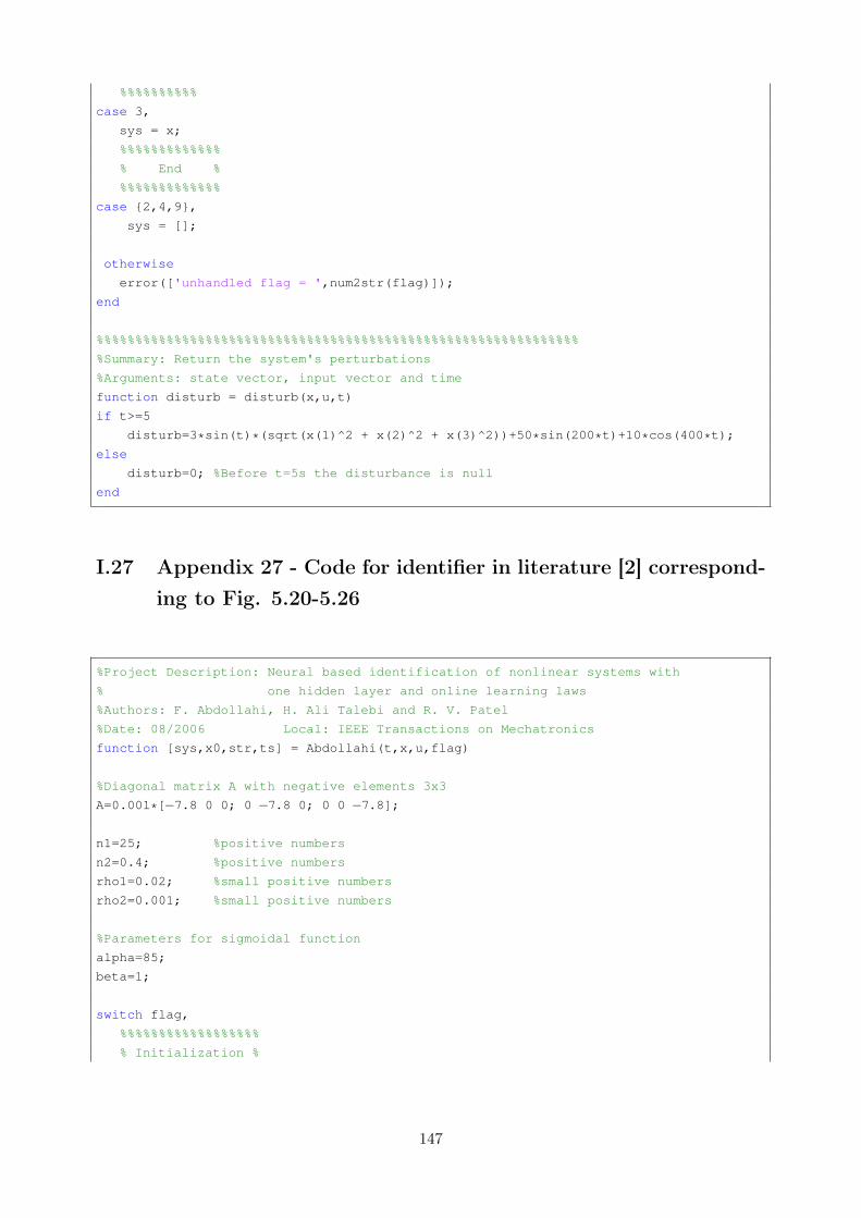
case 3,

sys = x;

%%%%%%%%%%%%%

% End %

%%%%%%%%%%%%%

case {2,4,9},

sys = [];

otherwise

error(['unhandled flag = ',num2str(flag)]);

end

%%%%%%%%%%%%%%%%%%%%%%%%%%%%%%%%%%%%%%%%%%%%%%%%%%%%%%%%%%%%%%

%Summary: Return the system's perturbations

%Arguments: state vector, input vector and time

function disturb = disturb(x,u,t)

if t>=5

disturb=3*sin(t)*(sqrt(x(1)^2 + x(2)^2 + x(3)^2))+50*sin(200*t)+10*cos(400*t);

else

disturb=0; %Before t=5s the disturbance is null

end

I.27 Appendix 27 - Code for identifier in literature [2] correspond-ing to Fig. 5.20-5.26

%Project Description: Neural based identification of nonlinear systems with

% one hidden layer and online learning laws

%Authors: F. Abdollahi, H. Ali Talebi and R. V. Patel

%Date: 08/2006 Local: IEEE Transactions on Mechatronics

function [sys,x0,str,ts] = Abdollahi(t,x,u,flag)

%Diagonal matrix A with negative elements 3x3

A=0.001*[�7.8 0 0; 0 �7.8 0; 0 0 �7.8];

n1=25; %positive numbers

n2=0.4; %positive numbers

rho1=0.02; %small positive numbers

rho2=0.001; %small positive numbers

%Parameters for sigmoidal function

alpha=85;

beta=1;

switch flag,

%%%%%%%%%%%%%%%%%%

% Initialization %

147

%%%%%%%%%%%%%%%%%%

case 0,

sizes = simsizes;

sizes.NumContStates = 45; %Number of Continuous States

sizes.NumDiscStates = 0; %Number of Discret States

sizes.NumOutputs = 39; %Number of Outputs

sizes.NumInputs = 3; %Number of Inputs

sizes.DirFeedthrough = 1;

sizes.NumSampleTimes = 1;

sys = simsizes(sizes);

x0=zeros(45,1); %Initial Conditions

x0(1:3)=5; %Initial conditions for estimated states

str=[];

ts=[0 0];

%%%%%%%%%%%%%%%

% Derivatives %

%%%%%%%%%%%%%%%

case 1,

%Identification Model and Learning Laws implementation

sys = [A*x(1:3) + [x(4:6)'; x(7:9)'; x(10:12)']*Sig(x, u, alpha, beta);

�rho1*norm(x_error(x, u))*x(4:6) + n1*w_term1(x, u, A, 1, alpha, ...

beta);

�rho1*norm(x_error(x, u))*x(7:9) + n1*w_term1(x, u, A, 2, alpha, ...

beta);

�rho1*norm(x_error(x, u))*x(10:12) + n1*w_term1(x, u, A, 3, alpha, ...

beta);

�rho2*norm(x_error(x, u))*x(13:23) + n2*v_term1(x, u, A, 1, alpha, ...

beta);

�rho2*norm(x_error(x, u))*x(24:34) + n2*v_term1(x, u, A, 2, alpha, ...

beta);

�rho2*norm(x_error(x, u))*x(35:45) + n2*v_term1(x, u, A, 3, alpha, ...

beta)];

%%%%%%%%%%%%%%%

% Outputs %

%%%%%%%%%%%%%%%

case 3,

sys = [x(1:33);

norm([x(4:6)'; x(7:9)'; x(10:12)'],'fro');

norm([x(13:23)'; x(24:34)'; x(35:45)'], 'fro');

norm([x(4:45)], 'fro');

norm((u(1)�x(1)));norm((u(2)�x(2)));norm((u(3)�x(3)))];

case {2,4,9},

sys = [];

otherwise

error(['unhandled flag = ',num2str(flag)]);

148

end

%%%%%%%%%%%%%%%%%%%%%%%%%%%%%%%%%%%%%%%%%%%%%%%%%%%%%%%%%%%%%

%Summary: Returns the state estimation error vector

%Arguments: state vector, input vector

function x_error = x_error(x, u)

X = [x(1); x(2); x(3)];

U = [u(1); u(2); u(3)];

x_error = X � U;

%%%%%%%%%%%%%%%%%%%%%%%%%%%%%%%%%%%%%%%%%%%%%%%%%%%%%%%%%%%%%%

%Summary: Returns nonlinear regressor vector

%Arguments: state vector, input vector and parameters for sigmoidal function

function Sig = Sig(x,u, alpha, beta) %Regressor

%Parameters for sigmoidal function

VZ = [x(13:23)'; x(24:34)'; x(35:45)']*[u(1); u(2); u(3); u(1)^2; u(2)^2; u(3)^2; ...

u(1)*u(2); u(3)*u(2); u(1)*u(3); u(1)*u(2)*u(3); 1];

%Regressor Vector

Sig=[(z(VZ(1), alpha, beta));

(z(VZ(2), alpha, beta));

(z(VZ(3), alpha, beta))];

%%%%%%%%%%%%%%%%%%%%%%%%%%%%%%%%%%%%%%%%%%%%%%%%%%%%%%%%%%%%%%

%Summary: Scalar sigmoidal function

%Arguments: VZ regressor term and parameters for sigmoidal function

function z = z(arg, alpha, beta) %Activation Function

z = alpha/(1 + exp(�beta*arg)) � 1; %Sigmoidal Function

%%%%%%%%%%%%%%%%%%%%%%%%%%%%%%%%%%%%%%%%%%%%%%%%%%%%%%%%%%%%%%

%Summary: Returns a vector containing the derivatives of the nonlinear NN regressor

%Arguments: state vector, input vector, matrix B and K, line, parameters for ...

sigmoidal function

function Sigdot = Sigdot(x,u, alpha, beta) %Regressor

%Regressor for activation function

VZ = [x(13:23)'; x(24:34)'; x(35:45)']*[u(1); u(2); u(3); u(1)^2; u(2)^2; u(3)^2; ...

u(1)*u(2); u(3)*u(2); u(1)*u(3); u(1)*u(2)*u(3); 1];

%Approximation using taylor series, this is the derivative of

%the regressor

Sigdot=[(z(VZ(1), alpha, beta))^2 0 0;

0 (z(VZ(2), alpha, beta))^2 0;

0 0 (z(VZ(3), alpha, beta))^2];

149

%%%%%%%%%%%%%%%%%%%%%%%%%%%%%%%%%%%%%%%%%%%%%%%%%%%%%%%%%%%%%%

%Summary: Returns the line from B*K*Xerro*S(VZ)

%Arguments: state vector, input vector, matrix B and K, line, parameters for ...

sigmoidal function

function w_term1 = w_term1(x, u, A, line, alpha, beta)

temp = (((x_error(x,u)')*inv(A))')*((Sig(x, u, alpha, beta))');

if line == 1

w_term1 = temp(1, :)';

end

if line == 2

w_term1 = temp(2, :)';

end

if line == 3

w_term1 = temp(3, :)';

end

%%%%%%%%%%%%%%%%%%%%%%%%%%%%%%%%%%%%%%%%%%%%%%%%%%%%%%%%%%%%%%

%Summary: Returns the line for Sdot(VZ)*W'*B*K*Xerro*Z'

%Arguments: state vector, input vector, matrix B and K, line, parameters for ...

sigmoidal function

function v_term1 = v_term1(x, u, A, line, alpha, beta)

W_est = [x(4:6)'; x(7:9)'; x(10:12)'];

X_est = [u(1); u(2); u(3); u(1)^2; u(2)^2; u(3)^2; u(1)*u(2); u(3)*u(2); ...

u(1)*u(3); u(1)*u(2)*u(3); 1];

temp = ((x_error(x,u)'*inv(A)*W_est*(eye(3)�Sigdot(x,u, alpha, ...

beta)))')*sign(X_est');

if line == 1

v_term1 = temp(1, :)';

end

if line == 2

v_term1 = temp(2, :)';

end

if line == 3

v_term1 = temp(3, :)';

end

I.28 Appendix 28 - Code for proposed identifier corresponding toFig. 5.20-5.26

The code is the same as Appendix 17.

150

I.29 Appendix 29 - Code to display the Fig. 5.20-5.26

%Displays the actual states and their estimations

set(0,'DefaultAxesColorOrder',[0 0 1; 1 0 0; 0 0 0]);

fsize=14;

figure;

plot(t, Xestimado(:,37),t, Xestimado1(:,37), 'LineWidth', 2 );

axis([0 10 �0.5 inf]);

set(0,'DefaultAxesFontSize', 17);

h=legend('Proposed Algorithm','Algorithm in [1]');

set(h,'FontSize',fsize);

xlabel('Time(s)','interpreter','latex','Fontsize',fsize);

ylabel('State Error Norm of x(t)','Fontsize',fsize);

%%%%%%%%%%%%%%%%%%%%%%%%%%

figure;

plot(t, Xestimado(:,38),t, Xestimado1(:,38), 'LineWidth', 2 );

axis([0 10 �0.5 inf]);

set(0,'DefaultAxesFontSize', 17);

h=legend('Proposed Algorithm','Algorithm in [1]');

set(h,'FontSize',fsize);

xlabel('Time(s)','interpreter','latex','Fontsize',fsize);

ylabel('State Error Norm of y(t)','Fontsize',fsize);

%%%%%%%%%%%%%%%%%%%%%%%%%%

figure;

plot(t, Xestimado(:,39),t, Xestimado1(:,39), 'LineWidth', 2 );

axis([0 10 �0.5 inf]);

set(0,'DefaultAxesFontSize', 17);

h=legend('Proposed Algorithm','Algorithm in [1]');

set(h,'FontSize',fsize);

xlabel('Time(s)','interpreter','latex','Fontsize',fsize);

ylabel('State Error Norm of z(t)','Fontsize',fsize);

%%%%%%%%%%%%%%%%%%%%%%%%%%

set(0,'DefaultAxesColorOrder',[0 0 0; 1 0 0; 0 0 0]);

figure;

plot(t, Xestimado1(:,34), 'LineWidth', 2 );

h=legend('Algorithm in [1]')

set(0,'DefaultAxesFontSize', 17);

set(h,'FontSize',fsize);

xlabel('Time(s)','interpreter','latex','Fontsize',fsize);

ylabel('Estimated Weight Norm W','Fontsize',fsize);

%%%%%%%%%%%%%%%%%%%%%%%%%%

151

figure;

plot(t, Xestimado1(:,35), 'LineWidth', 2 );

h=legend('Algorithm in [1]')

set(0,'DefaultAxesFontSize', 17);

set(h,'FontSize',fsize);

xlabel('Time(s)','interpreter','latex','Fontsize',fsize);

ylabel('Estimated Weight Norm V','Fontsize',fsize);

%%%%%%%%%%%%%%%%%%%%%%%%%%

152