MSc in Business Administration

Master thesis on topic: The impact of the financial crisis on innovation activity of public technology companies: evidence from Germany

Alisa Golomzina (s1358561)

a.golomzina@student.utwente.nl

School of management and governance

Business administration department

Dr. M. Ehrenhard (University of Twente)

Dr. A. Kock (TU–Berlin)

ENSCHEDE, AUG 27, 2013

2

Acknowledgements

I’m very grateful to my supervisors Dr. Alexander Kock and Dr. Michel Ehrenhard for

their encouragement and enormous support of this research. I also want to thank Mouna

Lara Saleh and Emily Rachel Parker for their valuable comments.

3

Abstract

This thesis aimed to explore the impact impaired by financial crisis 2008-2009 on

innovation activities of public technology firms in Germany. Specifically, the analysis

focused on the change in R&D intensity due to the crisis with respect to firm-specific

characteristics (size and age). The research also investigated the resulting influence of

this change on firms’ market-based performance. Through the longitudinal observation

of a panel of 110 German public companies attributable to technology sector, the

analysis rejected the suggestions of both pro-cyclicality in R&D investment and

positive relationship between R&D intensity and firm value. The following findings

were derived: 1) overall, public technology companies tend to persist their innovation

investment in spite of the crisis; 2) younger and smaller firms in general are more R&D

intensive that older and larger firms, in particular, smaller firms even increased their

R&D intensity during the crisis; 3) there are found to be industrial differences in

patterns of R&D investment; 4) market value is found to be negatively associated with

R&D investment during the crisis. Limitations of the analysis and perspectives for

future research are discussed.

.

4

Table of Contents

I. Introduction .................................................................................................................7

1.1. The relevance of the research..............................................................................7

1.2. Research question and the structure of the work .............................................8

II. Background for the research: overview of basic concepts ...................................10

2.1. Financial crises ...................................................................................................10

2.1.1. Financial crisis: definition, characteristics, taxonomy..................................10

2.1.2. Origins of financial crises .............................................................................13

2.1.3. Financial crisis 2007-2009: overview and theoretical explication................16

2.2. From innovation activity to R&D investment .................................................19

2.2.1. R&D investment: Defining the terms ...........................................................19

2.2.2. R&D investment: characteristics, sources of financing, effective measures 20

2.2.3. R&D investment and firm performance........................................................22

III. Theoretical framework: Crisis and innovation ...................................................25

3.1. Major effects of financial crises on firm performance and economic growth

.....................................................................................................................................25

3.2. Firms’ response to the financial crisis: pro-cyclical versus counter-cyclical

behavior in innovation investment ..........................................................................27

IV. Empirical analysis: Data and Method ..................................................................30

4.1. Research design: panel study ............................................................................30

4.1.1. Sample...........................................................................................................31

4.1.2. Data collection ..............................................................................................33

4.2. Variables .............................................................................................................35

4.3. Methodology .......................................................................................................37

V. Empirical analysis: Results .....................................................................................39

5.1. Exploring the data..............................................................................................39

5.2. Longitudinal analysis: R&D Intensity hypotheses..........................................47

5.3. Regression analysis: R&D intensity-Firm performance hypothesis .............56

VI. Summary and Conclusion......................................................................................61

5

Appendix A ....................................................................................................................63

Appendix B ....................................................................................................................64

Bibliography ..................................................................................................................65

List of Tables Table 1. Description of the preliminary sample based on the Credit Risk Monitor

database. ..................................................................................................................32  

Table 2. Final panel of firms available for the analysis. .................................................33  

Table 3. Variables and their description. ........................................................................35  

Table 4. Summary of the research methods and their links to hypotheses. ....................37  

Table 5. Descriptive statistics of key variables over the panel. .....................................40  

Table 6. Descriptive statistics of R&D intensity across industries. ................................44  

Table 7. Pairwise correlations of the key variables.........................................................47  

Table 8. Fixed-effects regression results for Tobin’s Q over the panel. .........................57  

Table 9. Fixed-effects regression results for the Return on Assets.................................58  

Table 10. Descriptive statistics for the measures of change in R&D..............................59  

Table 11. Regression results for Tobin’s Q in 2010. .....................................................59  

Table 12. Regression results for Tobin’s Q in 2011. ......................................................60  

Table 13. Correlation matrix of variables. ......................................................................63  

Table 14. Regression results for the Tobin’s Q in 2010, 2011 and 2012 with respect to

the change in the R&D intensity. ............................................................................64  

List of Figures Figure 1. The real GDP growth in Germany for the period 2003-2013..........................31  

Figure 2. Industrial composition of the panel. ................................................................39  

Figure 3. Distribution of the panel across Sub-sectors and Market Indices....................40  

Figure 4. Age characterisitcs across industries. ..............................................................42  

Figure 5. Size characterisitcs across industries. ..............................................................42  

Figure 6. Characterisitcs of R&D across over industries. ..............................................43  

Figure 7. Market indicators across industries. ................................................................45  

Figure 8. Performance indicators across industries.........................................................46  

Figure 9. The movement of the mean R&D intensity in the panel over time. ...............48  

Figure 10. The movement of the mean R&D Expenditure and Total Revenue in the

panel over time........................................................................................................48  

6

Figure 11. The movement of the mean R&D intensity in the panel with respect to size

effect........................................................................................................................50  

Figure 12. The movement of the mean R&D Expenditure in the panel with respect to

size effect. ...............................................................................................................50  

Figure 13. Decomposing the size effect on mean R&D intensity in the panel. .............51  

Figure 14. The movement of mean R&D intensity with respect to age effect................53  

Figure 15. The movement of mean R&D Expenditure (log) with respect to age effect. 54  

Figure 16. Overview of industrial patterns of R&D intensity in the panel over time.....55  

Figure 17. The movement of the mean R&D intensity over industries. ........................55  

7

I. Introduction

1.1. The relevance of the research

Scholars have different opinions regarding the roots of the recent financial crisis

2008-2009 and the recession that followed it. Some possible reasons mentioned in the

literature include: the collapse of the “financial bubble” as a part of a bigger structural

phenomenon (Perez, 2009), intellectual monopolization of the economy as one of the

reasons for the economic shock (Pagano & Rossi, 2009), the evidence of a middle-term

business cycle (Alvarez-Ramirez & Rodriguez, 2011), financial innovations in

competitieve banking system (Thakor, 2012). Regardless of cause, of major importance

is the significant negative effect of the crisis on the global economy (OECD, Guellec et

al., 2009).

Surprisingly, there is still a lack of theoretical and empirical research on the

impact of the recent financial crisis on the innovation activity of firms (both in terms of

investment in innovation and innovation performance). At the aggregated (national)

level the investment in innovations tends to be rather cyclical. The literature provides

some empirical evidence of this cyclicality from the US (Campello, Graham, & Harvey,

2010, p. 470), European Union (Archibugi & Filippetti, 2011, p. 1153), eight Latin

American countries (Paunov, 2012a, p. 24). But at the firm-level there is mixed

evidence of both cyclical and counter-cyclical behavior (e.g. Correa & Iootty, 2010;

Filippetti & Archibugi, 2011; Laperche, Lefebvre, & Langlet, 2011; Archibugi,

Filippetti, & Frenz, 2013). Moreover, the patterns of innovation performance seem to

differ from the patterns of innovation investment. For example, in Latin America while

the investment decreased significantly, introduced product innovations decreased in

average by more than 1% and process innovations increased more than 10% (Paunov,

2012a, p. 26). Several works also analyze the particular strategies firms implement to

respond to the crisis (Laperche et al., 2011; Mazzanti, Montresor, Antonioli, Bianchi, &

Pini, 2011).

The present analysis aims to fill the existing research gap by providing the

empirical evidence from German technology companies and contribute to the stream of

research in this field.

The relevance of exploring the interconnection between the financial crisis and

the innovation activity of firms naturally arises from the logic of economic

development. As suggested by J. Schumpeter in his theory of business cycles (1939),

major technological improvements are the drivers for the changes in long economical

8

cycles (Schumpeter, 1939, p. 83). Through a dynamic process of “creative destruction”

new technologies replace the old ones, shaping the economic development: “radical”

innovations create major disruptive changes, whereas “incremental” innovations

continuously advance the process of change (OECD/Eurostat, 2005, p. 30). Hence,

innovation activity contributes to economic development and growth. Financial crises,

on the other hand are believed to be the integral part of the business cycles (e.g. F. Allen

& Gale, 1998, p. 1248). Thus, the impact of the financial crisis on innovation activity

represents the feedback loop of innovations’ effects on the business cycle.

1.2. Research question and the structure of the work

The purpose of this thesis research is to investigate the impact impaired by

financial crisis 2008-2009 on the innovation activities of public companies within a

particular industrial sector (Technology) in Germany. Related literature suggests the

existence of sectoral patterns of innovation (e.g. Malerba & Orsenigo, 1997; Pavitt,

1999), thus it is interesting to explore the similarities or dissimilarities in the way firms

within one sector respond to the common exogenous shock. To the technology sector

the technology-intensive industries as included: telecommunication, communication

equipment, semiconductors, electrical engineering, mechanical/industrial engineering

etc.1 Technology sector is of particular interest since the mentioned industries are

named to be the most research and innovation intensive in Germany alongside with

automotive industry, pharmaceutics and biotechnology (Belitz, Clemens, & Cullmann,

2010, p. 13).

This analysis focuses on public companies, first of all, because of the

availability of corporate data. Moreover, public companies are often of larger size and

older age, thus the analysis might help to test the predictions of the theories dealing with

the size advantage and incumbency in relation to innovation activities (see, for example,

(e.g. Chandy & Tellis, 2000; Hill & Rothaermel, 2003). Germany is chosen because it is

one of the leading European innovators (Archibugi & Filippetti, 2011, p. 1166).

The central question of the analysis is formulated as follows:

How did German public technology companies change the scope of their

innovation activity in terms of R&D investment during the crisis 2008-2009?

More specifically, the following research questions needed to be addressed:

1 Based on the data from http://www.research-in-germany.de/ (last accessed 23.05.2013); http://www.crmz.com/Directory/CountryDES.htm (last accessed 05.08.2013)

9

1) What was the change in innovation investment before-during-after the crisis?

2) How did those changes influence the firms’ financial performance?

The thesis is organized as follows: Chapter II introduces the basic concepts for the

analysis, namely: financial crisis, innovation activity and R&D investment. In Chapter

III the author develops the theoretical framework for the analysis, exploring the

theoretical and empirical evidence of financial crises’ impact on firm performance and

innovation activity (reflected in R&D investment). Moreover, the author identifies the

general patterns of firms’ response to the crisis, discuss the possible determinants for

such a behavior and formulate the hypotheses for the empirical testing. Chapter IV

presents the research design for the empirical study and argues on sampling and data

collection procedure. Results of the empirical analysis are introduced in Chapter V. The

research concludes with the discussion of results and suggestions for the further analysis

in Chapter VI.

10

II. Background for the research: overview of basic concepts

2.1. Financial crises

2.1.1. Financial crisis: definition, characteristics, taxonomy

The analysis starts with a closer look at the phenomenon of financial crisis.

Financial crises are defined as “systemic disturbances to the financial system that

impede the system’s ability to allocate financial capital and disrupt the economy’s

capacity to function” (Visano, 2006, p. 3), therefore leading to severe financial and

economic distress. The term systemic refer to the collapse of the part or the whole

financial structure (Lagunoff & Schreft, 2001, p. 221). The dysfunction is characterized

by the unwillingness of investors to provide funding to the financial system (Thakor,

2012, p. 136) either directly or through financial intermediaries (e.g. banks). Sometimes

in the literature the term “banking panic” is used as a synonymous to “financial crisis”

(e.g. Gorton, 1988, p. 751; F. Allen & Gale, 1998, p. 1245), however, such a

terminology emphasizes the focus on banks and other financial intermediaries and

neglects the significance of, for example, financial markets in the process. To avoid this

misleading interpretation in the current work the term “financial crisis” is used.

Financial crises usually develop as a two-stage process: during the first (“run-up”)

phase (Brunnermeier & Oehmke, 2012, p. 3) the so-called “bubble” inflates and the

imbalances between the asset prices and their real values increase; after the bubble

impodes, the stage of actual crisis begins, during which the effects of the bubble's burst

spread to the other sectors and markets, often followed by a recession of the whole

economy (Franklin Allen & Gale, 2000, p. 236; Kindleberger, 2005, p. 12;

Brunnermeier & Oehmke, 2012, pp. 3–4). The term “bubble” defines here the situation

of a sustained mispricing of the financial or real asset (usually, real estate or security),

when the purchase of the assets are driven not by the expected rate of return on the

investment, rather by the anticipation of high profit from the asset's resale due to the

constant price increase (Kindleberger, 2005, p. 13; Brunnermeier & Oehmke, 2012, p.

12).

The general model of a financial crisis was described among the first by H.

Minsky within the “financial-instability hypothesis” (Minsky, 1982, p. 13)2. According

to this model, the potential crisis starts with the displacement (an exogenous shock such

as technical innovation or change in financial regulation), which is strong enough to 2 The model is well-elaborated in (Kindleberger, 2005, pp. 25–33), which the author refers to in the further analysis.

11

create an optimism among investors and generate the expectations of profit

opportunities and economic growth in a particular sector of economy (Kindleberger,

2005, pp. 25–26). This optimism leads to the expansion of the investment and credit

and, consequently, to the increase in assets price, which accelerates over time

(Brunnermeier & Oehmke, 2012, p. 12). Decoupling of the market prices from the real

values of the underlying fundamentals signals the forming of the bubble (Perez, 2009, p.

784; Barnes, 2011, p. 424). A bubble can inflate in such a way over a long period of

time - from 15 to 40 months (Kindleberger, 2005, p. 26). With the explosively growing

prices for the asset, the number of trading speculations takes off, creating the situation

of market euphoria, characterized by high interest rates and speed of payments

(Kindleberger, 2005, p. 31; Brunnermeier & Oehmke, 2012, p. 12). Abnormally high

profits attract new less sophisticated investors, thus spreading the euphoria to the other

markets (also internationally). At this stage more sophisticated investors might get

suspicious about the bubble nature of the boom and seek to reduce their positions by

selling the assets to the newcomers and take the profits (Brunnermeier & Oehmke,

2012, p. 13). The demand for the asset is heated up by those new investors, however,

the scope of the imbalances is too high at this stage, thus even a non-major (in respect to

the whole economy) “unusual event” (e.g. failure of a firm or bank) is enough to trigger

the burst of the bubble and catalyze the panic (Minsky, 1982, pp. 30–31; Kindleberger,

2005, p. 30). This turning point, a so-called “Minsky moment”, changes the

expectations of the market agents, first of all the borrowers of the investment capital,

and leads to increased rates of returns for the increased risk, inabilities to meet the debt

liabilities, defaults and insolvencies of both firms and banks (Kindleberger, 2005, pp.

31–33; Barnes, 2011, p. 424).

An important role in increasing and spreading the effects of the burst is attributed

to the “amplification mechanisms”, developed as the bubble builds up (Brunnermeier &

Oehmke, 2012, pp. 4–5; Brunnermeier, 2009, p. 78). Direct amplification mechanisms

(i.e. caused by direct contractual links between the agents) realize through domino

effects within a network of interconnected financial institutions (e.g. interbank loans) or

in “runs” of capital owners (e.g. massive withdrawing of deposits) (F. Allen & Gale,

1998, p. 1245; Brunnermeier & Oehmke, 2012, p. 5). Although the deposit insurance in

modern banking almost liquidates the risk of “bank runs”, other financial institutions,

like hedge funds, are still vulnerable to them (Brunnermeier, 2009, p. 96). Indirect

amplifications (i.e. caused by spillovers and externalities) realize through price

mechanisms (Brunnermeier & Oehmke, 2012, p. 5). At the borrower’s side, mutually

12

reinforcing “liquidity spirals” (“loss spiral” and “margin/haircut spiral”) take place

(Brunnermeier, 2009, pp. 92–93). They are caused by investors’ capital erosion due to

the price drop and simultaneous tightening of lending standards and margins, and lead

to fire-sales, pushing down prices and tightening funding even further (Brunnermeier,

2009, p. 78). At the credit side, the worsening financial situation of lenders, caused by

the burst, leads to: a) the restriction of lending capital through the reduction of the

quality monitoring of borrowers’ investment decision (“moral hazard in monitoring”),

and b) to the reservation of the funds for the own projects in anticipation of interim

shocks (“precautionary hoarding”) (Brunnermeier, 2009, p. 95). As many agents in

financial system act as borrowers and lenders at same time, this gives rise to the

network effects (Brunnermeier & Oehmke, 2012, p. 52). Concerns about the

counterparty credit risk (which does not even necessarily exist) lead to the failure of

multiple trading parties to cancel out offsetting positions, thus creating a so-called

“gridlock” (Brunnermeier, 2009, p. 78). If the bubble formation was financed by credit,

the amplification mechanisms are stronger due to the de-leveraging of investors, and

turn the bubble's burst into the financial crisis (Brunnermeier & Oehmke, 2012, p. 5).

Although each crisis has its unique features, in the way they develop they tend to

follow the above described general pattern (Kindleberger, 2005, p. 33). Some other

characteristics that are common in advance of a crisis include: shifts in financial

regulation; credit expansion and debt accumulation (Franklin Allen & Gale, 2000, p.

238; Davis, 2003, p. 15); increase in the number of financial innovations (Davis, 2003,

p. 15; Perez, 2009, p. 791; Thakor, 2012, p. 144); easing of entry conditions to financial

markets and concentration of risk (Davis, 2003, p. 15).

Different typologies are applied for the analysis of financial crises distinguish

them according to a variety of grounds, such as: by sector (public, private or corporate);

by object of speculation (financial or real assets); or by institutional spheres of finance

(banks or financial markets) (Visano, 2006, p. 3). However, there is no dominating

taxonomy. One of the approaches is to distinguish between banking crisis, currency

crisis and twin crisis (e.g. Kaminsky & Reinhart, 1999, p. 473; Franklin Allen & Gale,

2007a, p. 24). Banking crisis refers to the simultaneous collapse of many banks (or in a

broader sense – financial institutions); currency crisis describes the situation of

devaluation or revaluation caused by the large volumes of trade in foreign exchange

market (Franklin Allen & Gale, 2007a, p. 24). Twin crisis occurs when banking and

currency crises happen simultaneously (Franklin Allen & Gale, 2007a, p. 9). From the

perspective of decision-making of individual agents, Lagunoff & Schreft (2001) suggest

13

to distinguish between situations, when agents do not foresee the possibility of

contagious losses and get involved in “loss spirals” (Brunnermeier, 2009, p. 92) and

situations when agents have perfect foresight, and strategically and simultaneously shift

to less risky portfolios in anticipation of future losses (Lagunoff & Schreft, 2001, pp.

221–222). A very broad typology, suggested in (Davis, 2003, pp. 5–6), distinguishes

between 3 generic types of financial instability: 1) bank failures; 2) market-price based;

3) market-liquidity based. Bank failures refer to the defaults of financial credit

institutions due to the loan or trading losses, which lead to drying up of lending capital

and wider economic disruption. Domestic and international facets are distinguished

here. Market-based crises refer to the extreme volatility in market price due to the shift

in expectations among the market agents; characterized by involvement of institutional

investors as principals and their “herding” behavior. Market-liquidity crises are

identified as “protracted collapses of market liquidity and issuance”; more typical for

debt and derivative markets rather than equity of foreign exchange (Davis, 2003, pp. 5–

6).

2.1.2. Origins of financial crises

One of the most intrguing questions about the phenomenon of crisis is what

causes them. Minsky, the author of the general model of crisis described above,

suggested that the internal mechanisms of “capitalist economy”, reflected in the pro-

cyclical supply of credit and speculative financing, generate the environment

“conductive to instability” (Minsky, 1982, p. 36) and increase the likelihood of financial

crisis, thus emphasizing the inherent fragility of the market economy itself (Lagunoff &

Schreft, 2001, p. 221; Barnes, 2011, p. 426). Later works aimed to explore the nature of

this fragility more systematically and explain the occurrence of crises. The literature

provides three groups of theories, suggesting the following sources of financial crises

(Gorton, 1988, pp. 223–224; Franklin Allen & Gale, 2007a, p. 20; Thakor, 2012):

1. Crises arise from panics that could be unrelated to fundamentals in real

economy and are random events (Kindleberger, 1978, p. 14; Diamond & Dybvig, 1983,

p. 416);

2. Crises arise from shocks to economic fundamentals and are systematic events

(Gorton, 1988, p. 248; F. Allen & Gale, 1998, p. 1249);

3. Crises take place due to the interconnectedness of agents and the complexity of

the financial system (Leitner, 2005, p. 2925; Caballero & Simsek, 2009, p. 1).

According to the first view, the crises occur as a result of the financial “mania”

that have an episodic nature and don't explain the whole business cycle, rather describe

14

(own emphasis) the turning point from “final upswing to initial downturn”

(Kindleberger, 1978, p. 14). “Mania” is a typical situation of a bubble’s inflation and is

defined as a “frenzied pattern of purchases” (Kindleberger, 2005, p. 13), when investors

thrust to buy the asset before the price increase further. The use of the term “mania”

also emphasizes the irrationality of the investors’ behavior, resulting from the “mob

psychology” when most or all of the market participants change their view at the same

time and move as a “herd” (Kindleberger, 1978, p. 28). Irrationality, thus, leads to the

system’s collapse: trigger event (as described in the general model) starts the panic,

which then feeds on itself until the prices become low enough to attract investors again

or until the policy regulation influences the situation (Kindleberger, 2005, p. 33). This

view was developed by the multi-equilibrium model in (Diamond & Dybvig, 1983),

where the panic is a self-fulfilling process, which occurs if all the participants anticipate

(based on some exogenous event) the decrease in the value of their assets and try to

withdraw their funds (or sell assets). However, if there is no common expectation of

value decrease, only those who actually need the funds will withdraw them, hence, no

panic will start (Franklin Allen & Gale, 2007a, p. 6). The model is random, because the

exogenous event forming the expectations can be anything – “a bad earnings report, a

commonly observed run at some other bank, a negative government forecast, or even

sunspots” (Diamond & Dybvig, 1983, p. 410). Moreover, the authors argue that the

panic can start even without a displacement (like risky technology or currency),

described in the general model (Diamond & Dybvig, 1983, p. 416).

The alternative view in turn suggests the systematic component in crises origin

and argues that crises arise in response to the “unfolding economic circumstances” and,

hence, are integral part of the business cycle (F. Allen & Gale, 1998, p. 1248).

According to Gorton (1988), panics (and subsequent crises) result from the changes in

perceived risks estimated on the basis of prior information (Gorton, 1988, p. 248). Due

to the information asymmetry between the market agents (e.g. banks and depositors), to

assess their risks agents have to use some kind of aggregate information (Gorton, 1988,

p. 224). Such aggregate information might be presented, for example, by the seasonal

changes in short-term interest rates (“Seasonal Hypothesis”), unexpected capital losses

due to the failure of a large financial institution (“Failure Hypothesis”) or liabilities of

failed nonfinancial business, signaling about the downturn phase of the business cycle

(“Recession Hypothesis”) (Gorton, 1988, p. 231). As empirically tested in (Gorton,

1988), the panics are systematic events, caused by the “consumption smoothing

behavior on the part of cash-in-advance constrained agents”, thus linked to the business

15

cycle (Gorton, 1988, p. 248). In other words, when the market participants have reasons

to believe that economic fundamentals soon are likely to loose their values due to the

recession or depression (aggregate information), they will try to secure their positions

by selling the stocks at the financial market or withdrawing their deposits from the

banks (change in the perceived risk) (Franklin Allen & Gale, 2007a, p. 58). Mass sales

at the stock markets lead to the sharp fall in price; bank “runs” threaten banks with

insolvency. The resulting panic is similar to the “mania” view, however, the cause is

principally different (Franklin Allen & Gale, 2007b, p. 6).

The most modern view takes into account the network perspective of financial

systems and focuses on the interconnectedeness of agents and the inherent complexity

of the system as the main source of crises. Due to the holding of diversified portfolios,

financial positions of market agents are linked to each other in a way that return on an

agent's portfolio depends on the portfolio allocations of other agents (Lagunoff &

Schreft, 2001, p. 201). An initial shock to fundamentals in one sector or “region” (F.

Allen & Gale, 2000, p. 2) of financial system generate losses to the individual portfolios

of the agents of this particular sector, but due to the overlapping claims with the other

agents, the losses spread across the network and become a “contagion” (F. Allen &

Gale, 2000, p. 2; Lagunoff & Schreft, 2001, p. 250). The interconnectedness, however,

not only generates fragility of the financial system, but also provides more sustainable

agents with the opportunities to “bail out” their less lucky partners through the mutual

insurance, even though the latter can not “pre-commit to making payments” (Leitner,

2005, p. 2925). The contagion view was developed by Simsek & Caballero (2009) who

focus on the decision-making process of the financial institutions (Simsek & Caballero,

2009, p. 2). While in the usual situation it is enough for agents to collect the information

only about their direct partners, when the shock hit some part of the network, to reduce

the counterparty risk agents also have to increase their efforts, as well as the costs of

information collection (Simsek & Caballero, 2009, pp. 1–2). Since agents have to

understand more interlinkages, the complexity of the environments increases. With

complexity rises perceived uncertainty, making even healthy agents pull back in order

to protect themselves from the contagion cascade. This results in the erosion of market

liquidity and exacerbates the financial crisis (Caballero & Simsek, 2009, p. 2). The last

view focuses more on the reasons for the crisis development from panic, assuming the

initial shock is already introduced to the system. However, the nature of the initial

shock is less emphasized in those models.

16

2.1.3. Financial crisis 2007-20093: overview and theoretical explication

The recent financial cirsis, originated in the U.S. and spread globaly, provided

scholars with an outstanding opportunity to test the predictions of theoretical models.

Before the author turns to the opinions, supporting the views described above, it is

useful to trace the brief chronology of the turmoil.

From the late 90s, the U.S. and most other countries in the developed world

experienced almost a decade of low interest rates (Perez, 2009, p. 796; Barnes, 2011, p.

425). Availability of cheap loans encouraged both individuals and firms to borrow

freely. This also stimulated financial institutions sell off their existing mortgages to

others, the process known as “securitisation” (Barnes, 2011, p. 425). Starting from the

end of 2006, there appeared official statements from the world leading financial

institutions (e.g. European Cenral Bank, HSBC), claiming the instability of the sub-

prime mortgage market and world financial markets in general due to the overflood of

financial derivatives (Dolmetsch, 2008; ECB, 2013). The trigger for the liquidity crisis

was an increase in subprime mortgage defaults in the U.S., which was first noted in

February 2007 (Brunnermeier, 2009, p. 82). During the summer of 2007 U.S. market

experienced a full-scale crisis in the confidence of investors holding securitized

mortgages, which lead to the collapse of the inter-bank lending. Banks became reluctant

to lend because of the high risks of losses on subprime-related securities and their

derivatives. Due to the globalization of inter-bank lending the liquidity crisis spread to

other financial institutions in other countries (Barnes, 2011, p. 425). In September, 2008

heavily exposed to the sub-prime mortgage market American investment bank Lehman

Brothers filed for bankruptcy, prompting worldwide financial panic (Kingsley, 2012).

Despite the government-backed significant cash injections, the lack of liquidity, caused

by mistrust among banks, had spread from loans into commodities, bonds, and equity

markets (Chorafas, 2009, p. 260; Dolmetsch, 2008). “On 18 October 2008 India’s

Sensex had fallen by 48.1 percent; Hong Kong’s Hang Seng, 46.8 percent; Japan’s

Nikkei, 45.9 percent; Germany’s Dax, 43.7 percent; France’s CAC 40, 43.5 percent;

and Britain’s FTSE 100, 39.1 percent. Russia’s equity index had beaten all others,

falling by nearly 70 percent” (Chorafas, 2009, p. 260). From the end of 2008 the G20

countries started to develop coordinated policy response to the spreading crisis,

resulting in the stimulus package worth $5 tn introduced in April, 2009. In line with the

3 The time frame 2007-2009 refers to the U.S. chronology. In the following chapters the author refers to this crisis as “financial crisis 2008-2009”, indicating that it fully spread to Europe with the start of the panic in the second half of 2008.

17

government fiscal expansion central banks gradually cut the interest rates (Kingsley,

2012; ECB, 2013). As a response to government intervention, the economy showed

some expansion, which led International Monetary Fund to declare the start of recovery

from the crisis (IMF, 2009, p. 1). However, by spring 2010 Greece officially claimed

the need in the financial support, which signaled the start of Eurozone crisis and threw

the crisis from the private sphere to public with a major issue of sovereign insolvency

(Shambaugh, 2012, p. 157).

Scholars express different opinions regarding the financial crisis 2007-2009,

providing support for each of the theoretical view presented in previous section. Some

authors interpret the recent crisis as prove for a typical “bubble” and a following panic,

unrelated to the economic fundamentals: ”…the bubble was brought about by excessive

borrowing which led to the fragility of the financial system in which speculative and

Ponzi financial structures, at both the individual and firm level, could not be sustained”

(Barnes, 2011, p. 431). Barnes (2011) also emphisizes the important role of the

accounting information in the development of the panic, because understated provisions

for bad and doubtful debts forced the misleading investment decisions (Barnes, 2011, p.

432).

Other works provide support to the business cycle view, proving that the initial

U.S. subprime crisis had its origin in the “shock to fundamentals”, which led to the

credit crisis, panic and recession in line with the general model of financial crisis

(Gorton, 2009, p. 567). Perez (2009) connects the recent financial crisis (“easy-liquidity

bubble”) with the precedent internet mania and crash of the 1990s (“major technology

bubble”), arguing that those two episodes are structurally related and are endogenous to

the way the technological revolutions develop (Perez, 2009, p. 779-780). Moreover, the

empirical study of U.S. stock market dynamics found the evidence that financial crisis

2007-2009 coincides with the occurrence of a 22-year cycle in the Dow Jones index,

also suggesting the connection with the long-term business cycles (Alvarez-Ramirez &

Rodriguez, 2011, p. 1332).

Finally, in line with the financial interconnectedness view, Brunnermeier (2009)

notes that although financial crisis 2007-2009 in its development has been very similar

to a classical banking crisis, its distinctive features refer to the large extent of

securitization, “which led to an opaque web of interconnected obligations"

(Brunnermeier, 2009, p. 98).

The discussion about the origins of the recent financial crisis is ongoing and is

undoubtedly important because of the significant damage crises impair on the real

18

economy (Franklin Allen & Gale, 2007b, p. 9). The further analysis is therefore

dedicated to the exploration of the impact of financial crisis on the economy from the

perspective of innovations.

To sum up, Section 2.1. introduced the concept of financial crisis, provided the

overview of the financial crisis 2008-2009 and briefly discussed its theoretical

explications. The following section focuses on the other essential component for this

analysis, namely: innovation activity reflected in R&D investment.

19

2.2. From innovation activity to R&D investment

2.2.1. R&D investment: Defining the terms

This section defines the concept of innovation activity and concentrates on R&D

investment as a measure for it. According to the terminology, adopted by OECD,

“innovation activities include all scientific, technological, organisational, financial and

commercial steps which actually lead, or are intended to lead, to the implementation of

technologically new or improved products and processes” (OECD, 2002, p. 18;

OECD/Eurostat, 2005, p. 18). Innovation activities, thus, can include a very wide range

of proceedings, such as: identification of new concepts for change and improvement;

acquisition of technical information, know-how or intellectual property; purchasing or

development of relevant skills; reorganization of business systems; introducing new

methods of marketing and selling and others (OECD/Eurostat, 2005, p. 36).

An essential, although not exhaustive, part of innovation activity is research and

development (R&D). The term is defined as “creative work undertaken on a

systematic basis in order to increase the stock of knowledge […] and the use of this

stock of knowledge to devise new applications” (OECD, 2002, p. 30). The scope of

R&D covers three types of activities, namely: basic research (experimental or

theoretical acquiring of new knowledge “without any particular application or use in

view”), applied research (“directed primarily towards a specific practical aim or

objective”) and experimental development (“systematic work, drawing on existing

knowledge gained from research and/or practical experience, which is directed to

producing new materials, products or devices, to installing new processes, systems and

services, or to improving substantially those already produced or installed”) (OECD,

2002, p. 31). In other words, R&D represents the key resource input for the process of

creating innovations (Licht & Zoz, 1998, p. 331).

In order to measure the R&D efforts different indicators might be employed. As

R&D refers to the process of knowledge creation and application, it is useful to

distinguish between input and output measures. Input measures represent all kind of

resources invested in the R&D activity, while output measures indicate the subsequent

results (OECD, 2002, p. 17). The most common input indicators used in the literature

are R&D expenditures and R&D personnel (e.g. Licht & Zoz, 1998, p. 330; OECD,

2002, p. 20; Wang, Lu, Huang, & Lee, 2013, p. 146). R&D expenditures reflect the

spending on the research and development activities performed in-house and/or

externally, representing the financial capital invested in the innovation activity (OECD,

20

2002, p. 20; Moncada-Paternò-Castello, Ciupagea, Smith, Tübke, & Tubbs, 2010, p.

523; Wang et al., 2013, p. 146). R&D personnel indicator counts the physical number of

employees directly involved in the R&D activities (i.e. researchers, engineers etc.),

representing the human capital invested (OECD, 2002, p. 20; Wang et al., 2013, p. 146).

Other possible input indicators include facilities available for R&D, such as

standardized equipment, laboratory space and facilities, journal subscriptions or

standardized computer time. Those are, however, rarely used in the research (OECD,

2002, p. 22). Appropriate measuring of the R&D output is somewhat more challenging

task, as the special technical knowledge acquired by the firm and the economical and

social effects are not always quantifiable. The indicator of R&D output most commonly

used in the literature is patent applications, which represent the protectable (if granted)

result of successful research (e.g. Clark, Freeman, & Soete, 1981, p. 309; Licht & Zoz,

1998, p. 303; Wang et al., 2013, p. 145). Apart from patents the output might be

measured using bibliometrics, analysis of trade data and technology balance of

payments (OECD, 2002, p. 17).

The focus of this analysis is the innovation input represented in the financial

capital invested in the R&D. In the literature the terms “R&D investment” and “R&D

expenditures” are often used as synonymous (e.g. Moncada-Paternò-Castello et al.,

2010, p. 524). However, taking into consideration the strategic importance of R&D

efforts in developing and sustaining a competitive advantage for firms, it sounds more

appropriate to go for the term “investment” (Ehie & Olibe, 2010, p. 128). Thus, in the

further analysis to refer to the financial capital invested in research and development the

name “R&D investment” is employed.

2.2.2. R&D investment: characteristics, sources of financing, effective measures

R&D investment differs from the other types of investment in a variety of ways.

First of all, this investment is somehow embedded in the human capital of the

organization, because in practice more than half of the R&D spending refer to the cost

of high-qualified scientist and engineers (B. H. Hall & Lerner, 2010, p. 5). Through the

intellectual efforts of those employees the organisation absorbs and creates intangible

assets of firm-specific technological knowledge, which enables it to generate future

profits (Hashai & Almor, 2008, p. 1023; B. H. Hall & Lerner, 2010, p. 5). However, due

to the rather tacit nature of created knowledge, when the employee is gone, the

knowledge asset (and consequently, the R&D investment) is lost (B. H. Hall & Lerner,

21

2010, p. 5). This fact implies the high adjustment costs of R&D investment, making it

expensive for the firms to stop such investments (Paunov, 2012b, p. 27).

Secondly, the output of R&D investment is associated with high uncertainty,

which is especially high at the early stages of the projects (B. H. Hall & Lerner, 2010, p.

6). This uncertainly gives rise to the issues of, first, sources of funding capital for R&D

investment and, second, of its distribution among projects. The latter results in the

notion, that the projects with low probablity of success might still be worth financing

until their outcomes become more clear, thus R&D management requires rather

dynamic framework of real-options than a traditional evaluation of margin profits (B. H.

Hall & Lerner, 2010, p. 6; Paunov, 2012b, p. 27). The former referes to the problem of

assymetric information about the possible success of the innovation between the idea

owner and potential investor. Due to the strategic role of innovations, the disclosure of

firm-specific technical knowledge to the marketplace is not desirable by firms in order

to protect their ideas from imitation. This make it difficult for the potential investor (e.g.

bank) to evaluate the funding project and leads to the obstacles in aquiring of the

external financing for long-term highly uncertain R&D investment in comaprison with

ordinary (non-innovative) investment (B. H. Hall & Lerner, 2010, p. 9-10).

The above discussion implies the exceptional relevance of internal financing for

R&D investment. The major source for internal financing are positive cash flows (i.e.

retained earnings); this kind of internal equity financing is especially typical for

economies with well-developed financial markets and transparent ownership (such as

“Anglo-Saxon”) (B. H. Hall & Lerner, 2010, p. 23; Brown & Petersen, 2011, p. 659).

Internal financing is particularly important for young firms in high-tech industries who

have lower chances to get access to the debt capital due to the information problems,

skewed and highly uncertain returns and lack of collateral value (Brown, Fazzari, &

Petersen, 2009, p. 152). Alternative source of funding applicable for R&D investment is

the external equity financing through the stock markets (i.e. public share issues) (Brown

et al., 2009, p. 152). Due to the volatile nature of such funding sources, the exogenous

changes in the supply of internal or external equity finance (e.g. financial crisis) should

lead to the changes in R&D investment (Brown et al., 2009, p. 152).

Some characteristics of aggregated R&D investment are also worth mentioning.

At industry-level the composition of R&D investment is argued to be not homogeneous,

but rather follow “technological cycles” (Bhattacharjya, 1996, p. 445). Within those

cycles, independent to the exogenous shocks, the periods of a particular focus on long-

22

term oriented “research” activities are changed by the periods of short-term oriented

“development” activities (Bhattacharjya, 1996, p. 448).

A common measure employed in empirical research for firm’s R&D investment

is R&D intensity calculated as percentage of firm’s revenues expended on research and

development (e.g. Lin, Lee, & Hung, 2006, p. 679; L. A. Hall & Bagchi-Sen, 2007, p. 5;

Moncada-Paternò-Castello et al., 2010, p. 523). The relevance of this approach is

supported by the strong associations of R&D intensity with the measures of innovation

output, such as domestic and international patent applications and approvals (L. A. Hall

& Bagchi-Sen, 2007, p. 5). However, in this regard it is important to note the existence

of the time lag between the actual spending and the product revenue or profit generation

(L. A. Hall & Bagchi-Sen, 2007, p. 5; Wang et al., 2013, p. 146). High levels of R&D

intensity although not guarantee the generation of successful innovation, nevertheless

signal about strategic importance of innovation to the firm (Lin et al., 2006, p. 680). An

empirical study in biotechnology industry, for example, found significant relationships

between high levels of R&D intensity and high levels of research-based innovation, and

between low levels of R&D intensity and high levels of production-based innovation

(L. A. Hall & Bagchi-Sen, 2007, p. 12).

Among the factors shaping R&D intensity scholars name size, capacity for rapid

growth and a variety of “framework conditions”, such as entrepreneurial culture, IPR

regime, high taxation, access to finance and to adequate skills, social security regimes,

regulation of labor and capital markets etc. (Moncada-Paternò-Castello et al., 2010, p.

525). At the aggregated level, the research distinguishes between “intrinsic” and

“structural” effects, where the former refer to R&D intensity within industries, and the

latter concern the sector composition. Interestingly, EU is found to be inferior to the US

in the aggregated R&D intensity, which is explained by the differences in the

distribution of firms across sectors and company population. Despite its strong

specialization in automotive industry EU yields in IT hardware, electronics and

software. Moreover, in EU a relatively small number of companies perform larger

volumes of R&D; while in the US and in Japan the levels of R&D intensity are

distributed more broadly across many companies. (Moncada-Paternò-Castello et al.,

2010, p. 524).

2.2.3. R&D investment and firm performance

Concluding the discussion of R&D investment as a measure for innovation

activities, it is useful to trace the link between investment in research and development

23

and the overall functioning of firms. The literature suggests the positive impact of R&D

investment on firms’ financial performance (e.g. Griliches, 1986, p. 23; Ehie & Olibe,

2010, p. 128; Wang et al., 2013, p. 145). The general line of argumentation is as

follows: substantial investment in R&D is perceived as a risky strategy, therefore it is

associated with higher returns and, consequentially, is more attractive for the

shareholders in anticipation of better financial performance (Ehie & Olibe, 2010, p.

128). Three distinct streams of research focus on the following perspectives: 1) direct

impact of R&D output (i.e. patents) on firm-level performance; 2) the overall impact of

R&D activities (both input and output) on firms’ productivity and growth; and 3) the

contribution of the R&D investment to the market value of the firm (Toivanen,

Stoneman, & Bosworth, 2002, p. 39; Wang et al., 2013, p. 145). The overview of

related studies and major results are presented in (Wang et al., 2013, pp. 145–146).

The further discussion and empirical testing focuses on the latter perspective,

analyzing the impact of R&D investment on market-based valuation of firms. Market

value of assets is argued to be a useful approach in the assessment of private returns to

innovation, since the latter, expressed in R&D investment, represent the intangible

assets of the firms and, hence, are included in the bundle of total assets the firm

possesses. Assuming that financial market correctly price the firm’s assets (which is fair

for EU and the U.S.), it is, hence, possible to derive the marginal value of intangible

asset (innovation input) from the total firm value perceived by market (B. H. Hall, 1999,

p. 4).

A commonly accepted measure of market-based firm performance in the

empirical literature on R&D investment is Tobin’s Q (e.g. B. H. Hall, 1999, p. 6;

Toivanen et al., 2002, p. 40; Lin et al., 2006, p. 682). It is calculated as the ratio of

market value of assets to their book value and indicates the replacement cost of firms’

assets (Lev & Sougiannis, 1996, p. 109). Tobin’s Q, therefore, reflects the market

expectations of less quantifiable dimensions of performance, such as the portion of

intangible capital, to which R&D investment contributes to (Lin et al., 2006, p. 682). By

doing so, it allows to capture both short-term performance and long-term perspectives,

which are necessary to consider due to the long-term nature of innovation investment

(Lin et al., 2006, p. 682; Uotila, Maula, Keil, & Zahra, 2009, p. 247).

Empirical studies in general find significant positive relationship between R&D

investment and market value (e.g. Ehie & Olibe, 2010, p. 132). The U.S. data for

manufacturing firms shows that R&D investment is capitalized in the market value at

high rates (centered at 5-6), moreover, this relationships differ among industries (B. H.

24

Hall, 1999, p. 10). The evidence from the UK for the period 1989-1995 also suggests

that market positively values R&D investment, although this valuation doesn't’ show

any consistent trend over time and varies in coefficients from 2,5 to 5 (Toivanen et al.,

2002, p. 58). Surprisingly, the panel study of US technology firms for the period

between 1985-1999 hasn’t found the significant relationship between R&D intensity

and Tobin’s Q (Lin et al., 2006, p. 683). As a possible explanation for that the authors

emphasized the important role of commercialization efforts, which together with R&D

contribute to the value creation (Lin et al., 2006, p. 684).

However, the research of the R&D investment-market value link in the specific

situation of unfavorable economic environment is rather rare. Thus, the empirical

testing of this thesis might contribute to the better understanding of this relationship.

To sum up, Section 2.2. defined the term of innovation activity and the related

concept of R&D investment, providing the theoretical outlook of its characteristics,

measures and links to the firm performance. The following chapter aims to explore the

interconnection of two discussed phenomena – financial crises and innovation activity

reflected in R&D investment – and develops the theoretical framework for the further

analysis.

25

III. Theoretical framework: Crisis and innovation

3.1. Major effects of financial crises on firm performance and economic growth

From now on the author moves to the main focus of the study, namely: the impact

impaired by financial crises on firms’ performance with a special focus on their

innovation activity.

Financial markets and intermediaries function to facilitate the investment made by

firms, thus promoting economic growth. Hence, financial turmoil has a negative impact

on the firm performance, especially on those firms heavily dependent on debt capital

(Kroszner, Laeven, & Klingebiel, 2007, p. 188). Major negative effects related to the

financial collapse include: credit constraints, lack of liquidity, stock under pricing, drop

in demand, suboptimal allocation of investment and, consequentially, the slowdown of

economic growth.

First of all, financial shock either blocks completely or at least significantly

hinders the access of firms to “credit channel” (Akbar, Rehman, & Ormrod, 2013, p. 68;

Kroszner et al., 2007, p. 190). Increased real (or perceived) shortage of capital for

lenders leads to unwillingness of capital owners to finance even healthy firms. The

increased uncertainty about the riskiness of debt capital contributes to this reluctance

(Kroszner et al., 2007, p. 190). In particular, high-risk firms and firms with low share of

tangible assets are likely to be more sensitive to bank capital shocks (Popov & Udell,

2012, p. 160). Credit constraints refer to credit rationing in the capital markets (limited

credit availability), higher cost of borrowing, difficulties in initiating or renewing a

credit line (Campello et al., 2010, p. 471).

Credit constraints lead to the significant reducing of the costs. According to the

survey of 1050 companies by the end of 2008, “the average constrained firm in the U.S.

planned to dramatically reduce employment (by 11%), technology spending (by 22%),

capital investment (by 9%), marketing expenditures (by 33%), and dividend payments

(by 14%) in 2009” (Campello et al., 2010, p. 471). Decrease in employment, especialy

on a permanent basis, was also noticed, for example, for Eastern Europe (Ramalho,

Rodríguez-Meza, & Yang, 2009, p. 5). Other evidence of the credit constraints concerns

the burn of cash and cutting of dividends (Campello et al., 2010, p. 486). Credit

contrains (drastic decrease in new loans) also found to accelerate the withdrawal of

funds from the outstanding credit lines caused by the anticipated restriction of access to

them in the near future (Campello et al., 2010, p. 486; Popov & Udell, 2012, p. 159).

26

This is found to be true for firms with fewer internal funds, although such withdrwals

imposed higher costs (Campello, Giambona, Graham, & Harvey, 2011, p. 1947). To

hedge themselves from the negative impact of credit constraints, private firms tend to

hold cash and issue equity (Akbar et al., 2013, p. 68).

The other important negative effect of financial crisis reveals itself on the

downstream side of the firm performance in the significant drop in demand for products

and services and, consequently, decrease in sales (Ramalho et al., 2009, p. 2).

According to the survey among 1700 firms in Eastern Europe, more than 70% of the

firms of both production and service industries declared the sharp demand decrease

(Ramalho et al., 2009, p. 2).

Reduction of funds influence the amount of capital available for investment.

Firms have to cancel interesting and valuable investment or extend the investment plans

ex post, which affects firms' growth (Campello et al., 2010, p. 486; Fernández,

González, & Suárez, 2013, p. 2419; Gaiotti, 2013, p. 226). The inability to borrow

forces firms to search for other sources of financing. Possible alternatives include

internally generated cash flows, cash reserves or asset sales (Campello et al., 2010, p.

472; Borisova & Brown, 2013, p. 171). However, those measures are not always

optimal. For instance, fire sales of assets by the equity funds, who early had impared

losses from the investment in financial sectors are found to cause significant

underpricing of real stock (Hau & Lai, 2013, p. 393). Such a mispricing was found to

have a significant negative effect on both investment and employment.

The negative impact of crisis realizes not only in difficulties in access to

investment capital, but also in the composition of investments. Credit constraints

contribute to the “the asset allocation effect”, decreasing the share of investment in

intangible assets in favor of investment with high returns (Fernández et al., 2013, p.

2431). Moreover, the increased anticipated risk of liquidity shock due to the crisis,

reduces the firms’ willingness to engage in long-term investment (Aghion, Angeletos,

Banerjee, & Manova, 2010, p. 247).

Through the reduction of credit supply, decrease in intangible assets intensity and

contracting share of long-term investment financial crises hinders economic growth and

imposes higher volatility. (Aghion et al., 2010, p. 247; Fernández et al., 2013, p. 2420).

Those negative effects were found to be more significant in countries “whose more

financially developed system and better protection of property rights promote greater

growth during normal periods” (Fernández et al., 2013, p. 2431).

27

3.2. Firms’ response to the financial crisis: pro-cyclical versus counter-cyclical

behavior in innovation investment

In response to the unfavorable economic environment firms have two major

options: either to behave pro-cyclical (to cut costs, reduce and rationalize investment,

including innovation spending) or to stand up against the stream and to remain or even

increase the innovation activity, thus behaving counter-cyclical (Filippetti & Archibugi,

2011). The latter is explained by two opposite mechanisms, namely: creative

accumulation and creative destruction (Archibugi et al., 2013a, p. 303). Creative

accumulation refers to the process of continuous innovation on a regular basis of the

firms following the chosen technological trajectories and experiencing the path-

dependency (Nelson, 1982; Pavitt, 1999). Scholars argue that only few firms are able to

perform persistency in innovations (Geroski, Van Reenen, & Walters, 1997, p. 97),

however, such cumulative patterns are found to be greater “in those firms that (a) devote

a substantial budget to R&D and innovation, (b) concentrate on product innovations,

and (c) are large in terms of their size” (Archibugi et al., 2013; p. 304). The other

mechanism is a Schumpeterian creative destruction that refers to the emergence of new

innovators (‘entrepreneurs’) that might not be active before the crisis and who want to

take advantage of the crisis turmoil and to contest the market shares of incumbent firms

or to launch fresh markets (Francois & Lloyd-Ellis, 2003; Archibugi et al., 2013).

In general, R&D investment (and other long-term investment) tends to be rather

pro-cyclical and decline during the recessions, which is especially notable for the firms

facing tight credit constraints (Guellec et al., 2009, p. 6; Aghion, Askenazy, Berman,

Cette, & Eymard, 2012, p. 1001). The reason for pro-cycliality is that R&D investment

is financed mainly from the cash flows (as discussed in Section 2.2.2), which contracts

in the downturns due to the shrinking demand (Guellec et al., 2009, p. 6; Paunov,

2012a, p. 27). Moreover, credit constrains typical for financial crises makes it difficult

to get access to the external funding and, thus, also contributes to the decrease in R&D

spending (Paunov, 2012a, p. 27). The dependence of R&D investment on financial

constraints is found to be true also for the equity financing (i.e. issuing new stocks)

(Brown, Martinsson, & Petersen, 2012, p. 1527). However the evidence from the recent

crisis provides mixed support for both cyclical and counter-cyclical patterns. For

example, the survey of 500 multinational firms in the world, conducted by McKinsey,

indicates that 34% planned to spend less on R&D in 2009 while 21% planned instead to

increase spending (Guellec et al., 2009, p. 6). In turn, according to the EU-wide study

28

by Archibugi & Filippetti (2011) 65% of firms declared to have kept their innovation

investment unchanged in spite of the crisis (Archibugi & Filippetti, 2011, p. 1157).

In order to be consistent with the general theoretical predictions, for the present

empirical analysis the pro-cyclical hypothesis of R&D investment is formulated as

follows:

H1: Public technology firms show a decrease in innovation investment

during the crisis period in comparison to pre-crisis.

In line with the body of empirical research on R&D investment (as described in

Section 2.2.2), for the testing of this and the following hypotheses we will employ R&D

intensity as a measure of innovation investment.

Firms’ motivation to follow cyclical or counter-cyclical behavior is determined

by number of factors. Firm-specific factors influencing the firms’ decision to invest in

innovation regardless of the business cycle include: strategic orientation towards

innovation – especially following the exploration strategy, learning capabilities,

existence of in-house R&D facilities, network embeddings. Among industry-specific

determinants scholars name path dependent nature of the technology, technological

accumulation, dynamics of the demand and profit opportunities. Moreover, some

influential characteristics of institutional settings, such as national systems of

innovation play thier role (see Filippetti & Archibugi, (2011), Paunov, (2012),

Archibugi et al., (2013)).

A distinct stream of research discusses the significance of size and age in R&D

investment decisions during the economic downturn. There is some empirical evidence

that younger and smaller firms were more affected by the financial constraints

(Borisova & Brown, 2013, p. 171). Some recent studies of the crisis 2008-2009 provide

the support that larger and older firms are less vulnerable in terms of innovation

spending than the younger and smaller ones (Correa & Iootty, 2010, p. 20; Paunov,

2012, p. 32). In line with those findings the pro-cyclical hypothesis for R&D

investment distinguishes between size and age of the firms as follows

H2a: Larger firms show a less significant decrease than smaller firms.

H2b: Younger firms show more significant decrease, than older firms.

As already mentioned, industry-specific factors might influence the cyclical or

counter-cyclical behavior of firms (Archibugi, Filippetti, & Frenz, 2013b, p. 2). One of

the reasons for within-industry similarities is empirically supported in (Malerba &

Orsenigo, 1996, p. 470). By means of patent analysis across 49 technological classes the

29

authors argue that there exist patterns of innovation activities, which differ among each

other, but are systematically similar across countries for each class (Malerba &

Orsenigo, 1996, p. 451). Although those findings are proved to be true for innovation

output, it is interesting to explore whether the same logic is applicable to the innovation

input (i.e. R&D investment). When extending this proposition to the situation of crisis,

the following hypothesis is stated:

H3: The investment patterns during the crisis differ among industries.

Finally, it is useful to briefly discuss the impact of the crisis on the relationship

between R&D investment and firm’s market-based performance. Some empirical

studies exploring the impact of the economic disturbances on R&D intensity-market

value link showed the persistence of the positive relation although with lower influence

in face of the crisis (Ehie & Olibe, 2010, p. 133). This evidence suggests that the market

positively perceives the R&D efforts both in normal economic environment and in face

of crisis. Guided with those findings and the previously discussed positive contribution

of R&D investment to the firm’s value (see Section 2.2.3), the positive relationship

between them is anticipated with respect to the financial crisis. In line with the

empirical literature on the R&D investment - firm financial performance link (see

Section 2.2.3) Tobin’s Q is chosen as a measure of market-based financial performance.

The resulting hypothesis is developed as follows:

H4: Firms that increased their innovation investment during the crisis showed

better financial performance (higher Q) compared to firms, that didn’t change

their innovation investment.

Thus, Chapter III outlined the theoretical framework for the empirical analysis by

exploring the interactions among financial crises, firms’ performance and their

innovation activity. The following chapter presents the empirical framework of the

research, arguing on the data and method for the analysis.

30

IV. Empirical analysis: Data and Method

4.1. Research design: panel study

The main purpose of this analysis is to explore the patterns of investment in

R&D in response to the financial crisis 2008-2009 and compare them with pre-crisis

and post-crisis behavior. With a special focus on firm-specific characteristic (size, age

etc.) the author investigates the R&D spending across a panel of German public

companies (AGs: Die Aktiongesellsschaften), operating in technology sector. Taking

into account that financial crisis is not a single event, rather a developing process (as

described in Chapter 1.1) the analysis aims to explore its impact on corporate

innovation spending over a period time by employing the methods of longitudinal

analysis (Menard, 2008, p. 3; Rindfleisch, Malter, Ganesan, & Moorman, 2008, p. 34).

Longitudinal research design allows the measurement of change in phenomenon, and

moreover it allows controlling for individual unobserved heterogeneity (Brüderl, 2005,

p. 2; Menard, 2008, p. 3). This also differs this analysis from similar studies, that use

cross-sectional approach (Paunov, 2012a; Archibugi et al., 2013a).

As in some similar research on the impact of recent financial crisis on innovation

investment (Archibugi et al., 2013a, p. 306, e.g. 2013b, p. 4), the author starts the

observation from 2006, referring to 2006-2007 as a pre-crisis period, and carry the

investigation until 2012 in order to make use of the natural point of time the analysis is

conducted. Following the timeline of the financial crisis (as described in Section 1.3.),

the timeframe 2008-2009 refers to the actual period of crisis. Finally, the period from

2010 to 2012 refers to the post crisis period. The argument supporting this time frame is

the notion by IMF in the late 2009 (IMF, 2009, p. 1), when the global economy showed

some recovery from initial financial shock. However, as it further transformed in what

is often called “Eurozone crisis” (e.g. The Economist, 2013; The Guardian, 2010), it

would be more accurate to call this period a recession, following the 2008-2009

financial turmoil. The division of the time frame into the proposed also finds some

support when looking at the macro economical indicator of real GDP growth4 in

Germany over the past 10 years (Figure 1). Until 2006 there is an increase in growth,

slight decrease in 2007, then a significant drop in 2008-2009, followed by a sharp

increase in 2010 (partial economic recovery) and a steady decrease up to 2013 4 “Gross domestic product (GDP) is a measure of the economic activity, defined as the value of all goods and services produced less the value of any goods or services used in their creation. <…> For measuring the growth rate of GDP in terms of volumes, the GDP at current prices are valued in the prices of the previous year and the thus computed volume changes are imposed on the level of a reference year” (Eurostat, 2013).

31

(recession). To sum it up, the current analysis is designed as a longitudinal retrospective

panel study with a time frame 2006-2012 (T=7) (Menard, 2008, p. 6).

  Figure  1.  The  real  GDP  growth  in  Germany  for  the  period  2003-­2013  (Eurostat,  2013)5.    

4.1.1. Sample

In order to define the panel for the study the purposive non-probability sampling

approach was used (Babbie, 1998). This decision was made as the author seeked to

explore all the available organizations of a particular type (public companies) in a

particular industrial sector (Technology). The further adjustments to the size of chosen

sample were driven by the previous research (e.g. extending the range of industries) and

availability of data.

Preliminary population for the research consisted of 297 German public

companies, mentioned in the Technology sector according to Worldwide Directory of

Public Companies published by Credit Risk Monitor6. After a closer look at those

5http://epp.eurostat.ec.europa.eu/tgm/graph.do?tab=graph&plugin=1&language=en&pcode=tec00115&toolbox=typ (extracted on 05.08.2013) 6 http://www.crmz.com/Directory/CountryDES.htm (last accessed on 05.08.2013)

32

companies, the ones representing Computer Services and Software & Programming

were excluded from the sample, because they can hardly be further traced based on their

innovation output7. Further, comparing the Worldwide Directory of Public Companies

with a similar database8, it was noticed that the companies corresponding with

Mechanical Engineering industry, are mentioned in Capital Goods sector instead of

Technology. Those 63 companies were also added to the sample. Next, considering the

innovation intensity of ICT sector, 17 telecommunication companies (originally

classified in Service sector) were added. Thus, the preliminary sample for the research

counts 207 companies as illustrated in Table 1.

Table  1.  Description  of  the  preliminary  sample  based  on  the  Credit  Risk  Monitor  database.  

Sector Industry Number of Companies

Availability for Analysis

Technology

Communication Equipment

Computer Hardware

Computer Networks

Computer Peripheries

Computer Services

Computer Storage Devices

Electronic Instruments & Controls

Office Equipment

Scientific &Technical Instruments

Semiconductors

Software & Programming

23

5

6

9

44

3

27

4

13

37

121

-

-

Capital Goods Misc. Capital Goods 63

Services Communication Services 17

Total 372 207  

Further, the careful investigation of the preliminary sample was undertaken by

checking: first, the fact of existance and/or operation of each of 207 companies; second,

the presence of financial information available for analysis on the corporate web-site.

After this procedure, the panel of 110 companies was identified as follows (Table 2):

7 The current research project is to be continued with the analysis of the innovation output of the same panel. 8 http://www.research-in-germany.de/ (last accessed on 23.05.2013)

33

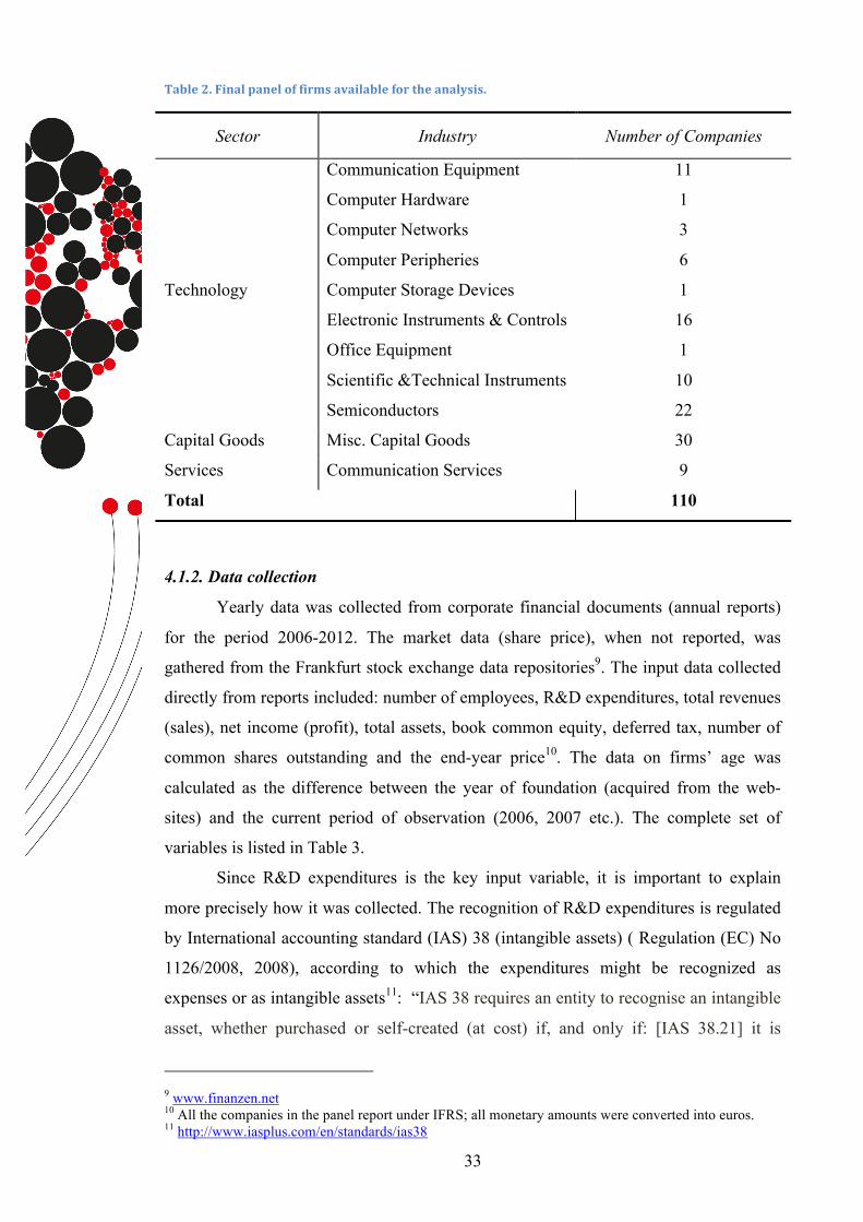
Table  2.  Final  panel  of  firms  available  for  the  analysis.  

Sector Industry Number of Companies

Technology

Communication Equipment

Computer Hardware

Computer Networks

Computer Peripheries

Computer Storage Devices

Electronic Instruments & Controls

Office Equipment

Scientific &Technical Instruments

Semiconductors

11

1

3

6

1

16

1

10

22

Capital Goods Misc. Capital Goods 30

Services Communication Services 9

Total 110

4.1.2. Data collection

Yearly data was collected from corporate financial documents (annual reports)

for the period 2006-2012. The market data (share price), when not reported, was

gathered from the Frankfurt stock exchange data repositories9. The input data collected

directly from reports included: number of employees, R&D expenditures, total revenues

(sales), net income (profit), total assets, book common equity, deferred tax, number of

common shares outstanding and the end-year price10. The data on firms’ age was

calculated as the difference between the year of foundation (acquired from the web-

sites) and the current period of observation (2006, 2007 etc.). The complete set of

variables is listed in Table 3.

Since R&D expenditures is the key input variable, it is important to explain

more precisely how it was collected. The recognition of R&D expenditures is regulated

by International accounting standard (IAS) 38 (intangible assets) ( Regulation (EC) No

1126/2008, 2008), according to which the expenditures might be recognized as

expenses or as intangible assets11: “IAS 38 requires an entity to recognise an intangible

asset, whether purchased or self-created (at cost) if, and only if: [IAS 38.21] it is

9 www.finanzen.net 10 All the companies in the panel report under IFRS; all monetary amounts were converted into euros. 11 http://www.iasplus.com/en/standards/ias38

34

probable that the future economic benefits that are attributable to the asset will flow to

the entity; and the cost of the asset can be measured reliably”. In case the described

recognition criteria are not met, “IAS 38 requires the expenditure on this item to be

recognised as an expense when it is incurred. [IAS 38.68]”. Moreover, “initial

recognition of research and development costs is prescribed as follows: charge all

research cost to expense [IAS 38.54]; development costs are capitalised only after

technical and commercial feasibility of the asset for sale or use have been established.

This means that the entity must intend and be able to complete the intangible asset and

either use it or sell it and be able to demonstrate how the asset will generate future

economic benefits. [IAS 38.57]”. For the purpose of the current research the author

considers the total amount of R&D expenditures reported, namely: the amount

recognized as expenses to the income plus net capitalized development costs for the

period. This approach is consistent with the Frascati Manual (OECD, 2002) and some

other research on R&D investment (e.g. Moncada-Paternò-Castello et al., 2010, p. 527).

Such a manual data collection is time-consuming, however, it provides higher

reliability of results due to the access to the primary source of data, it also allows to use

the specific set of indicators customized to the research questions and, moreover,

contributes to the data consistency. Alternatives to such a manual data collection might

be using the data from existing databases. For example, in case of similar research

authors use datasets from Community Innovation Survey (CIS), conducted by

Comission (Archibugi et al., 2013a, p. 306) or Innobarometer Survey, organized by

European Comission (Archibugi et al., 2013b, p. 4). The limitations of CIS are that it

is conducted not on the annual basis (every 2 years), besides the access to it is

problematic. Innobarometer is somewhat an aggregated dataset for the whole EU. Due

to its ex post nature the analysis has to exploit data obtained from completed survey

and, thus, can not select the data in accordance with the research objectives. It would be

useful for this analysis to use Compustat database12 because of the standardized

financial data (“one-stop-shopping”), unfortunately, there was no access to it.

Finally, the recognized limitations of data collection have to be mentioned. There

is a measurement error for 15 companies since they adapt different fiscal years (other

than January, 1 – December, 31) in their accounting policy. Out of 112 companies in the

sample 9 - report on September, 30; 4 on March, 31; 1 - on June, 30; and 1 - on May,

31. The data on those companies is included in the analysis as follows: fiscal year April,

12 https://www.capitaliq.com/home/what-we-offer/information-you-need/financials-valuation/compustat-financials.aspx (last accessed 27.08.2013)

35

1 20xx – March, 31 20xx+1 refers to the same fiscal year as January, 1 20xx –

December, 1 20xx. However, October, 1 20xx- September, 30 20xx+1 refers to the fiscal

year January, 1 20xx+1 – December, 31 20xx+1.

4.2. Variables

The major independent variable of interest is R&D investment measured in

R&D intensity as the ratio of R&D expenditures to total sales (Hall & Bagchi-Sen,

2007; Ehie & Olibe, 2010). Additionally, R&D expenditures in ablosulte values are

observed for the purposes of specific tests. Dependent variable is the Tobin's Q

(Bebchuk, Cohen, & Ferrell, 2009), measured as the ratio of market value of assets to

their book value (Kaplan & Zingales, 1997), (Gompers, Ishii, & Metrick, 2003),

(Bebchuk et al., 2009). The calculation of Tobin's Q components is adapted from the

Compustat data base items (Gompers et al., 2003), (Standard & Poor’s Compustat

Services, 2000). As an alternative dependent variable, reflecting the firm performance,

the ROA is examined. In line with the hypotheses, the control variables for the testing

models are Age (in logs) (Bebchuk et al., 2009), Size expressed in Number of

Employees and Total Revenues (both in logs) (Ehie & Olibe, 2010) and Leverage as a

proxy for financial risk (Kroszner et al., 2007, p. 221). Moreover, industry incorporation

and inclusion into one of the German stock index (DAX, TecDAX or CDAX13) is

observed (Gompers et al., 2003). In the Table 3 the detailed description of all the

variables is provided.

Table  3.  Variables  and  their  description.  

Variable Name Variable Type Construct Description

Dummies ID Independent The dummy code created to distinguish the

cases (companies).

Sector Independent The dummy code created based on the companies’ sector classification: 1=Capital Goods, 2= Services, 3= Technology

Industry Independent Industry Control

The dummy code created based on the companies’ industry classification: 1 - Communications Equipment; 2 -Communications Services; 3 - Computer

13 DAX (Deutscher Aktienindex) - market index, tracking the price development of the 30 largest and most actively traded German equities; TecDAX – index, reflecting the price development of the 30 largest technology shares in Prime Standard below DAX; CDAX (Composite DAX) - index that reflects the price development of all German shares across Prime Standard and General Standard (Deutsche Börse, 2013).

36

Hardware; 4 - Computer Networks; 5 - Computer Peripherals; 6 - Computer Storage Devices; 7 - Electronic Instruments & Controls; 8 Misc. Capital Goods; 9 - Office Equipment; 10 - Scientific & Technical Instruments; 11 Semiconductors

Market Index Independent Control The dummies representing the inclusion of the company into the Market Index (0=CDAX, 1=DAX, 2=TecDAX)

Input data Year Founded Interim The year of the enterprise foundation; used for

the calculating age at each observed period Number of

Employees Independent Size

control/Model

The size of the company reflected in the average number of employees for the period (in logs).

R&D

Expenditures Independent Model R&D Expenditures expressed in absolute values (in thousands EUR) in logs.

Total Revenue Independent Size

control/Model

The amount of total revenues reported in absolute values (thousands EUR) in logs.

Net Income Interim The net income (profit) expressed in absolute values (in thousands EUR)

Total Number of

Common Shares Interim The amount of the total outstanding shares of common stock.

Share price for

Common Stock Independent Control The market price for one share of common stock (end year price at XETRA) in absolute values (EUR).

Total Book

Assets Interim The amount of company’s assets expressed in absolute values (thousands EUR)

Book Common

Equity Interim The book common equity (shareholder’s equity less preferred equity) expressed in absolute values (thousands EUR).

DefferedTax Interim Balance sheet deferred taxes expressed in absolute values (thousands EUR).

Computed data

37

Age Independent Age

control/Model

The age of the company in years at each observed period (in logs).

R&D Intensity Independent Model R&D intensity expressed as the ratio of R&D Expenditures to Total Revenues

Leverage Independent Control Financial leverage (Debt-to-Equity) calculated as a ratio of total book assets less common equity to common equity

Book Value of

Equity Interim

Book value of common equity (the sum of Book common equity and deferred taxes) expressed in absolute values (thousands EUR).

Market Capitalization Interim

The market value of common stock expressed as the market share price times the total amount of shares outstanding (in logs).

Market Assets Interim

Market value of assets, where market value is a book value of assets plus market value of common stock less the book value of common equity, expressed in absolute values (thousands EUR).

ROA Dependent Model Return on the company assets expressed as the ratio of Net income to total assets.

Q Dependent Model Tobin’s Q expressed as a ratio of market value of assets to book value of assets.

4.3. Methodology

To test the hypotheses H1-H3 the author employs the method of unobtrusive

research by descriptive analysis of the available statistics on the panel over the course of

T=7 (Babbie, 1998, p. 322). To test the H4 regression analysis is implemented.

Table 4 describes the research methods to be implemented to answer the

research questions stated in hypotheses above (see Section 3.2.) together with the key

measures and sources of data. Table  4.  Summary  of  the  research  methods  and  their  links  to  hypotheses.    

Hypothesis Method Measures

H1: public technology firms decrease innovation investment during the crisis.

H2a: larger firms show less decrease than smaller firms. H2b: younger firms show more significant decrease,

Longitudinal panel

observation

Independent variables: R&D

expenses (as absolute value)

R&D intensity (as relative to

company’s revenue for the period)

Control variables: Age, Size,

Industry

38

than older firms. H3: investment patterns differ across industries. H4: innovation investment during the crisis positively influences firm performance.

Regression

Analysis

Independent Variables: R&D

Intensity, Change in R&D intensity

Dependent Variables: Firm

performance (expressed as Tobin’s

Q and ROA)

Thus, Chapter IV introduced the empirical framework for the analysis, argued

on research design, data, sample and methods employed. The following chapter presents

and discusses the results of the empirical testing over the panel in order to support the

hypotheses developed within the theoretical framework.

39

V. Empirical analysis: Results

5.1. Exploring the data

In the following section the author moves to the empirical analysis of the panel

of German technology companies (n=110, T=7). For the longitudinal panel analysis

Stata software is used with implementation of the insturments of xtset analysis

(StataCorp., 2011).

Figure  2.  Industrial  composition  of  the  panel.    

Figure 2 and 3 present the overview of the panel structure from the perspectives

of industrial and sub-sectoral composition and firm's distribution across market indices.

Out of 11 industries represented in the panel, the majority of firms are concentrated in

7: Misc.Capital Goods (i.e. Industrial Engeneering – 28%), Semiconductors – 20%,

Electronic Instruments & Controls – 14,5%, Communication Equipment – 10%,

Scientific & Technical Instruments – 9%, Communication Services – 8% and Computer

Peropherials – 5%. Those attract the primary attention of the analysis. Interestingly, the

panel is dominated by CDAX firms, while DAX and TecDAX companies together have

less than 15%. That means that most of the firms are of small and medium size and are

not that actively traded at the stock market.

40

Figure  3.  Distribution  of  the  panel  across  Sub-­sectors  and  Market  Indices.        

The author starts the analaysis by looking at the descriptive statistics of the data

(Table 5). Summarized descriptive statistics for longitudinal panel decompose the mean

variable xit into a between (xi) and within (xit = xi + x, the global mean x being added

back in order to make the results comparable). The overall and within are calculated

over N firms-years of data. The between is calculated over n firms, where N refer to

firms-years, n – to firms, T – average number of years the variable was observed

(StataCorp., 2011).

Table  5.  Descriptive  statistics  of  key    variables  over  the  panel.  

Variable Mean Std. Dev. Min Max Observations Age overall 50.47 61.98 -4.00 443.00 N = 770 between 62.19 -1.00 440.00 n = 110 within 2.00 47.47 53.47 T = 7 Number overall 9 766.04 48 306.35 0.00 472 500.00 N = 695 of between 46 473.29 39 950.00 416 621.40 n = 108 Employees within 3 094.62 -20 655.39 65 644.61 T-bar = 6.43 Total overall 1 919 616.00 9 707 548.00 0.00 87 300 000.00 N = 709 Revenue between 9 347 547.00 700.50 77 300 000.00 n = 110 within 577 244.60 -2 960 956.00 11 900 000.00 T-bar = 6.45

41

R&D overall 91 289.97 487 549.10 0.00 5 024 000.00 N = 565 Expenditure between 442 616.50 59.00 4 338 571.00 n = 98 within 53 352.05 -452 376.70 776 623.30 T-bar = 5.77 R&D overall 0.06 0.06 0.00 0.49 N = 563 Intensity between 0.07 0.00 0.35 n = 98 within 0.03 -0.13 0.25 T-bar = 5.74 Financial overall 1.79 6.05 -40.32 135.01 N = 696 Leverage between 2.54 -2.23 19.67 n = 110 within 5.50 -37.59 117.13 T-bar = 6.34 Share overall 14.05 20.00 0.24 257.10 N = 657 Price between 15.04 0.38 73.92 n = 107 within 12.63 -35.73 209.08 T-bar = 6.14 Market overall 1 567 025.00 8 525 041.00 810.06 88 100 000.00 N = 657 Cap between 7 906 744.00 2 104.22 67 000 000.00 n = 107 within 1 493 085.00 -9 048 611.00 22 700 000.00 T-bar = 6.14 Book-to- overall 0.86 0.88 -2.13 11.98 N = 654 Market between 0.63 -1.08 3.72 n = 107 within 0.67 -1.27 10.36 T-bar = 6.11 ROA overall -0.02 0.32 -5.88 0.69 N = 706 between 0.19 -1.16 0.19 n = 110 within 0.26 -4.73 1.16 T-bar = 6.42 Tobin's Q overall 1.43 0.84 0.13 7.48 N = 654 between 0.62 0.46 3.71 n = 107 within 0.56 -1.03 6.79 T-bar = 6.11

The values of some variables (Age, Number of Employees, Total Revenue,

R&D Expenditure and Market capitalisation) are not normally distributed, thus it is

useful to use the median as a cenrtality measure for them rather than mean. For the

further analysis they are taken in logs. It's is also interesting to decompose the data

across the structural components and compare the results with the overall panel. Figures

4-8 illustrate the industiral differences of the companies on the key variables.

Firms show significant difference of Age across the industries. While

Misc.Capital Goods (i.e. industrial engineering) and Office Equipment are close to the

panel mean, most of the other industries vary in the range from 10 to 20 year (Scientific

Instruments are a decade older). This is in line with the nature of the technological

development: IT-related industries raised much later than industrial engineering.

42

Figure  4.  Age  characterisitcs  across  industries.    

Figure  5.  Size  characterisitcs  across  industries.    

43

Both size characteristic across industries are generally consistent with each

other and in line with the Age: younger industries (e.g. Computer Hardware or

Computer Networks) are respectively have less revenues and employees and the other

way around (e.g. Industrial Engineering). Interestingly, Communication Services being

smaller in headcount show unproportionally high revenues. Office Equipment show the

inverse pattern, however, due to the very little representation in the panel, this is not

much informative.

Figure  6.    Characterisitcs  of  R&D  across  over  industries.    

R&D related indicators show interesting behaviour. While in absolute values

R&D expenditures are low or moderate (e.g. Computer Networks, Communication

Equipment, Semiconductors), in terms of R&D Intensity those firms show the highest

values (8-9%). In turn, Misc.Capital Goods, that shows high volumes of R&D

investments has only moderate intensity (4%). This fact proves the relevance of using

the R&D intensity as a measure of engagement in innovation activity.

44

   Table  6.  Descriptive  statistics  of  R&D  intensity  across  industries.

Industry Variable Mean Std. Dev. Min Max Observations

1 Communication Equipment overall 0.09 0.08 0.00 0.34 N = 58 between 0.10 0.03 0.30 n = 10 within 0.02 0.03 0.17 T-bar = 5.8

2 Communication Services overall 0.01 0.02 0.00 0.11 N=34 between 0.02 0.00 0.05 n=7 within 0.01 0.00 0.07 T-bar = 4.86

3 Computer Hardware overall 0.00 0.00 0.00 0.00 N=2 between . 0.00 0.00 n=1 within 0.00 0.00 0.00 T=2

4 Computer Networks overall 0.09 0.09 0.00 0.18 N=4 between 0.08 0.00 0.12 n=2 within 0.06 0.00 0.15 T=2

5 Computer Peripherals overall 0.08 0.10 0.01 0.49 N=33 between 0.12 0.02 0.35 n=6 within 0.04 -0.06 0.22 T-bar = 5.5

6 Computer Storage Devices overall 0.01 0.01 0.01 0.03 N=5 between . 0.01 0.01 n=1 within 0.01 0.01 0.03 T=5

7 Electronic Instr. & Controls overall 0.05 0.04 0.00 0.18 N=78 between 0.04 0.01 0.15 n=14 within 0.01 -0.01 0.10 T-bar = 5.57

8 Misc. Capital Goods overall 0.04 0.04 0.00 0.24 N=150 between 0.04 0.00 0.15 n=25 within 0.01 -0.02 0.13 T=6

9 Office Equipment overall 0.01 0.00 0.01 0.02 N=7 between . 0.01 0.01 n=1 within 0.00 0.01 0.02 T=7

10 Scientific & Technical Instr. overall 0.09 0.06 0.01 0.24 N=59 between 0.06 0.02 0.20 n=10 within 0.02 0.04 0.13 T-bar = 5.9

11 Semiconductors overall 0.08 0.07 0.00 0.36 N=133 between 0.06 0.00 0.20 n=21 within 0.04 -0.11 0.27 T-bar = 6.33

The benchmark study of the 1000 most R&D intensive EU and non-EU

companies (Moncada-Paternò-Castello et al., 2010, p. 527) suggests to distinguish

between high-intensive (more than 5%), medium-high (2-5%), medium low (1-2%) and

45

low intensity (below 1%) industries. High R&D intensity industries comprise

pharmaceuticals & biotechnology, health-care equipment & services, technology

hardware & equipment, software & computer services and leisure goods. Medium-high

include automobiles & parts, aerospace & defence, electronics & electrical equipment,

industrial engineering & machinery, chemicals, personal goods, household goods,

general industrials, support services and travel & leisure. Medium-low R&D intensity:

food producers, media, oil equipment, general retailers, tobacco, mobile and fixed line

telecommunications. Low R&D intensity: as oil & gas, industrial metals, banks,

construction &materials, food & drug retailers, beverages, industrial transportation,

mining, electricity and multiutilities (Moncada-Paternò-Castello et al., 2010, p. 527). As

seen from the Table 6, the results over the panel are absolutely consistent with the

suggested benchmark classification.

From the perspective of market performance, the most valued industries in terms

of share prices are Computer Peripherals, Electronic Instruments & Controls, Industrial

Engineering and Semiconductors. At the same time only the latter two show consistent

pattern of market capitalization.

 

Figure  7.  Market  indicators  across  industries.    

46

Figure  8.  Performance  indicators  across  industries.  

Lastly, the group of performance indicators provide some interesting insights.

Such, ROA of virtually half of the panel is negative, which is logically might be

explained as a impact of crisis on financial performance (negative profits). Even in case

of positive returns, the values are still low (less than 5%). Computer Hardware and

Computer Storage Devices show comparatively much better results, although, as

mentioned earlier, due to the low representation their results might be not reliable.

Tobin’s Q is distributed mostly equally among the industries with an exception of

highly overvalued Computer Networks. Most of the other industries show the value

consistent with the panel’s mean of 1,43, which reflects in general positive attitude of

the market towards the technology intensive firms.

To make one step further in understanding the panel it is neccessary to look at

the correlations existing among the key variables as described in Table 7 (for the full

correlation matrix see Appendix A). Strong correlation between Number of Employees

and Total Revenues supports the choice of both as size controls. As it was noticed, Age

and Size correlate with each other, in particular Age and Number of Employees.

Moreover, R&D Expenditures show significant positive correlation with the size

controls, while R&D Intensity reveals negative correlation with age. Interesting

relations shows the share price, correlating with both age and size and, besides, with

47

R&D Expenditure. Tobin's Q correlation with the share price might be explained by the

market component of the ratio. Table  7.  Pairwise  correlations  of  the  key  variables.    

Variables 1 2 3 4 5 6 7 8 9 10

1 Age 1.00

2 Number of Employees

0.26* 1.00

3 Total revenue 0.19* 0.99* 1.00

4 Industry -0.09 -0.10* 1.00

5 Market Index 0.16* 0.18* 1.00

6 R&D Expenditure 0.20* 0.89* 0.82* 0.16* 1.00

7 R&D Intensity -0.18* -0.08 0.18* 1.00

8 Leverage -0.13* 1.00

9 Share price 0.22* 0.27* 0.25* 0.13* 0.30* -0.13* 1.00

10 ROA 0.09 -0.22* 0.14* 1.00

11 Tobin's Q -0.12* 0.09 0.35* -0.10

Results printed for p >.05, * - for p > .01

5.2. Longitudinal analysis: R&D Intensity hypotheses

Descriptive statistics provide somehow a snapshot of the data. To make use of the

longitudinal research design and to answer the research question, we should look at the

data over time. Analysis of longitudinal data typically concentrates on the changes in

mean values over the given time period and on relation of those changes to the

covariates (Menard, 2008, p. 204). Thus, to test the first hypothesis (H1) we trace the

change of panel’s mean R&D intensity over the course of 7 years (2006-2012). Figure 9

illustrates that.

The mean R&D intensity indeed shows a decline in 2008 (when the crisis

occurred), generally supporting the predictions of H1. Interestingly, in 2009, which

refers to the crisis period in our definition, it also has a sligh increase, followed by the

decrease until 2011, which is in line with the recession period. However, the overall

fluctuations of R&D intensity are in range of less than 1% and, therefore, might be not

very significant. As R&D intensity depend on R&D Expenditures and Total Revenue,

it’s useful to track their behavior as well (Figure 10). Both variables (in logs) don’t

show any significant change in spite of crisis. According to this visualization, firms in

the panel seem to remain the intensity unchanged, which contradicts the expectations of

H1.

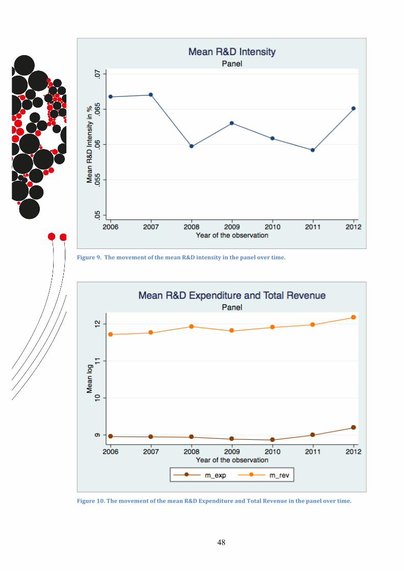
48

Figure  9.    The  movement  of  the  mean  R&D  intensity  in  the  panel  over  time.  

Figure  10.  The  movement  of  the  mean  R&D  Expenditure  and  Total  Revenue  in  the  panel  over  time.  

 

49

To test the decrease in R&D intensity during the crisis period the author

implements the two-sample t-test, distinguishing between the period before the crisis

(2006-2007) and period during (and after) the crisis (2008-2012) (Hamilton, 2006, p.

148). There is no significant differences in the mean intensity for pre-crisis period

(M=0.07, SD=0.07) and during and after crisis (M=0.06, SD=0.06); t (561)=0.91, p =

0.36314. The result is also robust for the unequal variances t (232)=0.82, p = 0.41. The p

is high, therefore there is no reason to reject null hypothesis. Similarly, there are no

significant differences in the means of R&D expenditures and Total Revenues:

(M=8.95, SD= 2.08) before the crisis and (M=8.97, SD= 2.18) during and after the

crisis; t (560)= -0.81, p=0.94 for R&D Expenditures and (M=11.74, SD= 2.14) for pre-

crisis versus (M=11.95, SD= 2.07) during and after crisis; t (705)= -1.22, p=0.22 for

Total Revenues. These results suggest that the technology firms in the panel didn’t

decrease their R&D intensity in spite of crisis. Thus, the H1 is not supported.

Further, Hypotheses 2a and 2b seek to test the impact of size and age effects on

R&D intensity with regard to the crisis. To test H2a we distinguish between larger and

smaller firms, based on the EU-definition of small and medium enterprises (EC, 2003,

p. 39). Firms with a headcount less than 250 employees and an annual turnover less

than 50 millions euro, are considered as small in the panel. Respectively, those with

more than 250 employees and 50 million euro revenues are considered as large. Figure

11 illustrates the movement in mean R&D intensity over period of study with respect to

the joint size effect of both Number of Employees and Total Revenue. Lager firms are

very similar in their pattern to the mean over the panel, showing almost no change in

R&D intensity in spite of crisis. Smaller firms have much more curious pattern: first,

they are on average more research intensive (2% difference); second, they show only a

slight decrease by the 2008 year (comparable on speed with larger firms in 2007-2008),

but then showing a significant 3% increase up to the 2010 (i.e. during the crisis). This

behavior is very interesting and contradicts the expectations of the H2a.

At the same time, mean R&D Expenditure doesn't show any notable responce to

the crisis circumstances when controling for size (Firgure 12). Both larger and smaller

firms behave similar to the panel's mean, smaller firms just show a little more persistent

decline.

14 Here and further the results are reported at 95% confidence level, unless the different is stated.

50

Figure  11.  The  movement  of  the  mean  R&D  intensity  in  the  panel  with  respect  to  size  effect.  

Figure  12.  The  movement  of  the  mean  R&D  Expenditure  in  the  panel  with  respect  to  size  effect.  

   

51

To check the robustness of the size effect the author looks at the impact of each

size control separately (Figure 13). While larger firms tend to present the same intensity

pattern, which is still close to the overall panel mean, smaller firms are more sensitive to

the size controls. When distinguished by the headcount, the pattern follows the

cumulative one, just somehow smothely and less extreme. However, when controling

for size by means of log revenues, the pattern looks differently. That might be explained

by the difference in the volatility level of revenues and employment, when the former

might change faster than the latter, although they are strongly connected as proved by

the pairwise correlation.

 Figure  13.  Decomposing  the  size  effect  on  mean  R&D  intensity  in  the  panel.  

In order to test the significance of size effect on R&D intensity, we again

employ the analaysis of variances. First of all, we look at the separate effects of each

control on overall R&D intensity by implementing a two-sample t-test. Depending on

the number of employees, larger and smaller firms indeed differ in their mean R&D

intensity, in particular smaller firms are more R&D intensive than larger ones: (M=0.08,

SD=0.08) for smaller firms versus (M=0.06, SD=0.06) for larger at t (561)=2.78, p =

0.006. When taking the Total Revenue as a measure for size, the results are consistent

and even more notable in case of smaller firms: (M=0.10, SD=0.09) for smaller firms

52

versus (M=0.05, SD=0.05) for larger at t (561)=2.78, p < 0.001. To test the effects of

size differences with regard to the crisis, two-way ANOVA test is used, by looking at

the interaction of each size control with the crisis variable (before and during/after)

(Hamilton, 2006, p. 152). The results yielded again the significant main effect for both

size controls (F (1, 559)=6.81, p=0.01 for Number of Employees and F (1, 559)=36.29,

p <0.001 for Total Revenues), while the main effect of crisis was not significant (F (1,

559)=0.40, p=0.53 and F (1, 559)=0.25, p=0.62 for Number of Employees and Total

Revenues respectively). Moreover, the interaction effect was not significant in both

cases (F (1, 559)=0.04, p=0.85 and F (1, 559)=0.06, p=0.80 for Number of Employees

and Total Revenues, respectively). This indicates that when controlling for number of

employees and total revenues separately, R&D intensity of firms differs with respect to

size characteristic. Specifically, smaller firms are more intensive than larger and the

impact of difference in total revenues is more notable. However, in this case the crisis

doesn’t seem to cause significant disproportions in mean R&D intensity among the

groups of larger and smaller firms.

The next step is to test the joint effect of the both size controls on the R&D

intensity and its response to the crisis. By implementing two-way ANOVA we model

the effect of number of employees, total revenues and their interaction on intensity.

Variance test yields the significant main effect of total revenues as a size control (F (1,

559)=34.24, p <0.001), while the impact of number of employees in the joint model is

smoothened and doesn’t have a significant main effect on intensity (F (1, 559)=1.32, p

=0.25). Furthermore, the interaction effect of both controls is insignificant on overall

intensity (F (1, 559)=0.15, p =0.70. Finally, we add the crisis variable into the model

and test for the significance of interaction effect of the joint size control and the crisis.

Interestingly, the joint model provides now the support for the crisis effect (F (1,

555)=9.41, p =0.02) on intensity, indicating that mean R&D intensity differs before and

after the crisis with respect to size. Moreover, the results yield the significant effect of

interaction between number of employees and total revenues (F (1, 555)=14.98, p

<0.001), indicating the difference in R&D intensity between large and small firms.

Lastly, there is found a significant main effect of interaction between both size controls

and the crisis variable (F (1, 555)=6.12, p < 0.001). These results suggest that with

respect to the joint size controls, financial crisis matters for the differences in R&D

intensity among small and large firms. Specifically, firms with lower headcound and

smaller revenues show increase in R&D intensity during the crisis (M=0.08, SD=0.08

before the crisis versus M=0.10, SD=0.09 after the crisis), which is larger than for firms

53

with more employees and higher revenues (M=0.05, SD=0.05 versus M=0.06, SD=0.05

before and after the crisis, respectively). These results contradict the propositions of

H2a, which although predicted the difference in responce to the crisis depending on

firm's size, but expected the other direction of change in R&D intensity. Thus, H2a is

rejected.

In order to test H2b, the analysis distinguishes between older and younger firms

based on the mean log age in the panel. Firms, whose log age is smaller than the mean

log age, are considered as younger; firms with log age larger than the mean log age, are

considered as older. Figure 14 illustrates the impact of age effect on the mean R&D

intensity over time; Figure 15 presents the same effect on R&D expenditure.

Figure  14.  The  movement  of  mean  R&D  intensity  with  respect  to  age  effect.  

According to the mean behavior on the graph, younger firms indeed decrease the

R&D intensity more sharply in the period 2006-2011 – in 2,5%, slowing down during

the crisis (2008-2009). Older firms, in turn, steadily increase the intensity rate by 1%

over the same period.

54

Figure  15.  The  movement  of  mean  R&D  Expenditure  (log)  with  respect  to  age  effect.  

Similarily to the size effect, the author tests the significance of this hypothesis by,

first, comparing the age differences over the panel and, secondly, evaluating the impact

of the crisis. The results of the t-test support the significant differences in mean R&D

intensity among younger and older firms, indicating that younger firms are more

intensive: (M=0.08, SD=0.08) for smaller firms versus (M=0.05, SD=0.05) for larger at

t (561)=5.90, p < 0.001. When introducing the crisis variable in the two-way ANOVA,

we yield the significant main effect of age (F (1, 559)=35.77, p <0.001), but, again, not

significant main effect of both crisis and their interaction (F (1, 559)= 0.52, p =0.47 and

F (1, 559)= 2.49, p =0.11 respectively). In other words, although younger and older

firms do significantly differ in their R&D intensity, those differences are not getting

more notable during the crisis. Thus, the H2b is not supported.

In accordance with H3 the existense of industrial patterns in R&D intensity is

expected. Figure 16 provides the overview of the industrial patterns of R&D intensity in

the panel. One can notice that the patterns are not identical in line with the H3, however

it is not clear how the R&D intensity moves over time. To track its development it’s is

useful to have a closer look at the mean values over time (Figure 17).

55

Figure  16.  Overview  of  industrial  patterns  of  R&D  intensity  in  the  panel  over  time.    

Figure  17.  The  movement  of  the  mean  R&D  intensity    over  industries.  

56

Looking at the means across industries15 it is possible to identify 3 generic types

of behavior: decrease, increase or no change in R&D intensity during the crisis period in

comparisons to the pre-crisis. Computer Peripherals, Communication Equipment and

Semiconductors show a decrease in 2008-2009 in comparison with the levels of 2006-

2007, although Communication Equipment demonstrate faster recovery by 2010. In

contrast, R&D intensity levels within Electronic Instruments & Controls and Scientific

&Technical Instruments even increases in crisis period when compared to pre-crisis.

Finally, Communication Services and Misc.Captial Goods, both with comparatevely

low intensity levels, don't show any significant movements.

In order to test the significance of this hypothesis we implement one-way

ANOVA test (Hamilton, 2006, p. 150). Ananlysis of variances shows that the effect of

industry involvement on the mean R&D intensity is significant, F (10, 552) = 9.67, p

<0.001. In particular, Scheffé multiple-comparison test indicates the significant contrast

between Communication Equipment (M=0.09, SD=0.08) and Communication Services

(M=0.02, SD=0.02), p <0.001 and Misc. Capital Goods (M=0.04, SD=0.04), p = 0.004.

Scientific & Technical Instruments (M=0.09, SD=0.06) and Semiconductors (M=0.08,

SD=0.07) both have a significant variance from Communication Services (M=0.02,

SD=0.02) and from Misc. Capital Goods (M=0.04, SD=0.04), p = 0.001 and p < 0.001

respectively. Lastly, Computer Peripherals (M=0.08, SD=0.10) differs significantly

from Communication Services (M=0.02, SD=0.02), p =0.02. Hence, we have different

groups of industries based on their R&D intensity, thus H3 is supported.

5.3. Regression analysis: R&D intensity-Firm performance hypothesis

In order to test the final hypothesis H4 concerning the impact of the R&D

investment on firm performance in the face of crisis environment, we build a refression

model over the panel. First of all, it's useful to model the overall impact of R&D

intensity on the firm 's financial performance, using the two proxies for it – Tobin's Q

and ROA. Based on the Hausman test (StataCorp., 2011, p. 720), the coefficients for

both Q and ROA regressions are systemic, thus a fixed-effects (within) model describes

them better than a random-effect model. Table 8 presents the results of the regression.

15 The graphs are not informative for the Computer Hardware, Computer Networks, Computer

Storage Devices and Office Equipment industries, therefore they will be ignored in the further illustration.

57

Table  8.  Fixed-­effects  regression  results  for  Tobin’s  Q  over  the  panel.  

Tobin's Q 1 2 3 4 β t β t β t β t

Constant 2.28 4.38 4.29 3.89 5.99 5.00 5.64 4.74 (0.52) (1.11) (1.20) (1.19)

R&D Intensity -3.69* -3.34 -4.77* -3.30 -4.18* -2.91 -4.23* -3.00 (1.10) (1.44) (1.44) (1.41)

Log R&D Expenditures -0.07 -1.15 0.18* 2.37 0.17* 2.34 0.15* 2.03 (0.06) (0.07) (0.07) (0.07)

Log Number of Employees -0.78* -6.66 -0.72* -6.19 -0.71* -6.20 (0.12) (0.12) (0.11)

Log Total Revenue 0.10 0.76 0.17 1.25 0.15 1.14 (0.14) (0.14) (0.13)

Log Age -0.83* -3.42 -0.63* -2.59 (0.24) (0.24)

Leverage 0.01 -0.89

(0.01)

R2 (within) 0.04 0.18 0.20 0.20 R2 (between) 0.00 0.06 0.05 0.06 R2 (overall) 0.00 0.07 0.05 0.05 No. observations 532 524 524 520 No. groups 95 93 93 93 Standard errors are reported in parentheses. * - indicates the significance at the 95% level.

The regression is built in 4 steps (Models 1-4), where first only the R&D

investment is considered (1), then the size controls introduced (2), next – the age control

(3) and finally – the leverage control (4). Based on the goodness of fit, R2, models (3)

and (4) have the best explanatory power out of all, although still only 20% of Tobin’s Q

are explained. Since it is a panel, similarly to the descriptive statistics (see Table 5 in

5.1) we distinguish between within, between and overall effects. For the fixed-effects

regression R2 within is an ordinary R2, while the others are just correlations squared,

thus we concern R2 within the most (StataCorp., 2011, p. 456). Further, for the within

regression the relevant is Number of observations, representing the total amount of

firm-years, not the Number of groups (actual number of firms involved in the

regression). It seen from the Table 8, that R&D intensity has a robust significant

negative impact on market-based firm performance. Other significant factors, that

determines Tobin’s Q are R&D Expenditure, Number of Employees and Age.

To test the impact of R&D investment on the alternative measure of

performance, we run the similar regression for Return of Assets (Table 9).

58

Table  9.  Fixed-­effects  regression  results  for  the  Return  on  Assets.  

Return on Assets (ROA) 1 2 3 4 β t β t β t β t

Constant 0.55 2.33 (0.24)

R&D Intensity -2.12* -4.19 -2.01* -2.84 -1.66* -2.34 -1.64* -2.31 (0.51) (0.04) (0.71) (0.71)

Log R&D Expenditures -0.05 -1.76 -0.02 -0.67 0.03 -0.81 -0.02 -0.64 (0.03) (0.04) (0.04) (0.04)

Log Number of Employees -0.13* -2.25 -0.11 -1.66 -0.11 -1.86 (0.06) (0.06) (0.06)

Log Total Revenue 0.07 1.03 0.11 1.65 0.11 1.64 (0.07) (0.07) (0.07)

Log Age -0.39* -3.29 -0.40* -3.37 (0.12) (0.12)

Leverage -0.01 -1.70

(0.00)

R2 (within) 0.07 0.08 0.10 0.11 R2 (between) 0.02 0.00 0.03 0.03 R2 (overall) 0.01 0.00 0.01 0.01 No. observations 558 550 549 545 No. groups 97 95 95 95 Standard errors are reported in parentheses. * - indicates the significance at the 95% level The explanation power of this model is rather weak (only 11% at best), but since

it’s just an alternative measure, it is not the focus of the analysis. What’s more

important is that it also demonstrates a significant persistent impact of R&D intensity

and a weaker influence of Age as well. The major conclusion of the performed

regressions is as follows: R&D investment, measured as R&D intensity, has a

significant negative impact on firm performance: the increase in R&D intensity leads to

the decrease in returns.

To reflect the influence of R&D investment on firm performance in face of crisis

as stated in the H4, the author models the change in intensity for the 3 respective time

periods: “before” (the change between 2007 and 2006), “crisis” (the change between

2008 and 2007) and “after” (the change between 2009 and 2008)16. Taking in the

account the lagged nature of R&D investment, the author models the impact of the 16 This distinguishing attempts to grasp the impact of change in R&D ininvestment for the each point of time in the crisis time frame; in line with the research design, the «after» period refers to the general crisis period, however, the term «after» aims to reflect the fact that this period happened after the intial shock in the economic environment, which we call here «crisis» and mark as the difference between 2008 and 2007.

59

change in intensity on the Tobin’s Q for the last three years of the study (Q2010, Q2011

and Q2012, respectively). Table 10 presents the descriptive statistics for these variables.

    Table  10.  Descriptive  statistics  for  the  measures  of  change  in  R&D         intensity  in  face  of    crisis  and  Tobin’s  Q.  

Variable Obs Mean Std. Dev. Min Max

Independent

before 73 0.007 0.032 -0.128 0.135 crisis 79 -0.003 0.038 -0.278 0.075 after 78 0.006 0.035 -0.213 0.099

Dependent

Q2010 100 1.43 0.79 0.70 5.94 Q2011 101 1.28 0.67 0.13 4.68 Q2012 84 1.36 0.68 0.42 4.71

As already proved by the H1, there is only a very small insignificant descrease

in R&D intensity during the crisis (the difference between 2008 and 2007 is negative).

However, of the interest for the analysis is the impact of this change on the firm

performance. To test it, we build a regression model. Tables 11 and 12 show the

regressions for Q2010 and Q2011, since they had more obsevations and higher R2 (for

the full regression see Appendix B).

Table  11.    Regression  results  for  Tobin’s  Q  in  2010.  

Tobin's Q 2010 1 2 3 4 β t β t β t β t Constant 1.44 13.50 1.45 14.75 1.54 18.76 1.54 17.10 (0.11) (0.10) (0.08) (0.09)

before 5.88 1.76 -8.64 -1.86 (3.35) (4.65)

crisis -5.73* -2.22 -11.28 -1.77 (2.58) (6.37)

after -14.43* -6.28 -12.14* -3.69 (2.30) (3.29)

R2 0.04 0.06 0.35 0.41 Adjusted R2 0.03 0.05 0.34 0.38 No. Observations 69 76 75 66 Standard errors are reported in parentheses. * - indicates the significance at the 95% level

60

Table  12.  Regression  results  for  Tobin’s  Q  in  2011.  

Tobin's Q 2011 1 2 3 4 β t β t β t β t

Constant 1.18 17.52 1.20 18.64 1.28 20.68 1.25 21.23 (0.07) (0.06) (0.06) (0.06)

before 4.20* 2.01 -4.28 -1.42 (2.09) (3.01)

crisis -5.90* -3.55 -2.75 -0.64 (1.66) (4.27)

after -8.46* -4.94 -8.20* -3.81 (1.72) (2.15)

R2 0.06 0.15 0.26 0.36 Adjusted R2 0.04 0.14 0.25 0.33 No. Observations 66 73 73 63 Standard errors are reported in parentheses. * - indicates the significance at the 95% level Models (1) – (3) in each table show the individual impact of change in intensity

on the respective Q, while Model (4) demonstrates the joint impact. For both years

(2010 and 2011) the change in R&D intensity after the shock (2009-2008) has a

significant negative effect on firm performance reflected in Tobin's Q. Interesting

results are yielded for 2011: the change in R&D before the crisis is positively assosiated

with firm performance, while when the shock occurs, the influence becomes negtive

and increases with time. However, this relationship is not robust and disappears in the

joint model. To sum up, the increase in R&D spending in face of crisis leads to worse

performance. That contradicts the expectations of H4, which is therefore rejected.

Chapter V dealt with the empirical testing of the developed theoretical

propositions within the suggested research design. Out of 5 formulated hypotheses, only

H3 is fully supported with statistical testing, while H1, H2a, H2b and H4 have to be

rejected. In particular, for H2a the theoretical predictions about factors of change in

R&D intenstity (size) were true, while the direction of change (decrease) was proved to

be reverse. In the following chapter the results of the conducted theoretical and emprical

analysis are summarized and discussed and the concluding comments are derived.

61

VI. Summary and Conclusion This thesis reseach aimed to explore the effect that the recent financial crisis

2008-2008 impaired on the innovation activity of public technology firms and related

financial performance. Built on the theoretical body of knowledge about the financial

crises, innovation activity and R&D investment as a measure for it, the author attempted

to develop the theoretical framework which might possibly explain the nature of the

relationshiop between cirisis and innovation. More specifically, she hypothesized how

financial crisis hinders private investment in R&D and what are the possible effects of it

on firm's market value. In oder to test empirically the propositions of the theoretical

framework, the author collected financial data on the panel of German public firms

attributable to the technology sector. The results of the empirical analysis are more than

surprising.

First of all, the main hypothesis predicting the pro-cyclical behavior of R&D

investment in face of crisis didn't find empricial support. The analysis showed that firms

in the panel didn't significantly decrease their R&D intensity during the period of

financial crisis in comparison with the level of R&D intensity before the crisis. This

result is very interesting and provides a support for the “creative accumulation” view

(e.g. Archibugi et al., 2013a). It shows that technology firms, for whom the specific

technological knowledge is a strategically valuable asset, are more likely to be

persistent in their innovation activity in spite of the economical fluctuations. In this way

the conducted analysis contributes to the stream of reseatch on persistency of

innovations (e.g. Geroski et al., 1997; Archibugi et al., 2013b).

Next, the longitudinal panel analysis allowed to derive valuable insights about

the impact of firm-specific characterstics on innvation. The empirical findings over the

panel showed the evidence that size and age matter for R&D intensity. More

specifically, it was statistically proved that younger and smaller firms are more

intensive in their R&D invesment than older and bigger firms. As the impact of crisis

didn't find significan support over the panel, it is reasonable to conclude that these

differences preserve even in case of unfavorable economic environment (financial crisis

in our research). Moreover, when controlling for both factors of size (number of

employees and total revenues) smaller firms even showed the increase in R&D

intensity. It was also found that in general the effect of revenues as a factor for size is

more significant than the number of employees. These results contribute to the literature

exploring the influence of size and age on innovation activity (e.g. Cohen & Klepper,

62

1996; Chandy & Tellis, 2000; Hill & Rothaermel, 2003). In line with the theoretical

predictions the panel analysis also proved the industiral differences in R&D intensity,

which is found to be significant over time.

Even more interesting results were derived for the relationship between R&D

investment and market value of firms. Market-beased performance was found to be

strongly negatively assosiated with R&D intensity over the panel. In other words, the

increase in R&D leads to descrease in market percived value. The same is true for

return on assets, although with comparatively lower impact. Firm performance is also

assosiated with size and age in the following way: yonger and smaller (in terms of

headcount) show better market-based performance (regression coefficients are

negative), while in the ROA story only age matters. Interestingly, financial leverage as a

proxy for financial rist didn't show any significant influence on the performance for

both Tobin's Q and ROA. Furthermore, the change in R&D intensity is significantly

negatively associated with market-based performance during the crisis: firms who

increase their research and development intensity, experience worse market

performance. These findings are in contrast with the empirical evidence in the literature,

arguing for the positive relation between R&D and market value (e.g. B. H. Hall, 1999;

Toivanen et al., 2002). In this was this analysis provides the new insights that the crisis

situation seems to inverse the relationship between R&D investment and market

evaluation of the firm.

Thus, the major conclusion of the conducted analysis is as follows: in spite of

the financial crisis technology firms in Germany tend to persist their innovation activity

as reflected in R&D investment even if the financial market doesn't support it.

With regard to the generalization and implications of the results the author is

mindful about the subjective sampling as a limitation of the study. As a possible

improvement the robustness check testing for the adjustments in the industry

involvement might be useful.

To conclude, this thesis has focused only on the input dimension of the innovation

activity affected by crisis, namely on R&D investment and its intensity. In order to

complete the analysis of the financial crisis’ impact on the innovation activity of

German public technology firms it would be also be beneficial to consider innovation

output. The author intends to pursue further research on this topic by investigating the

patent activity of the firms in the chosen sample during the same period.

63

Appendix A Table  13.  Correlation  matrix  of  variables.  

1 2 3 4 5 6 7 8 9 10 11 12 13 14 15 16 17 18 1 Market Index 1.00 2 Sector -0.09 1.00 3 Industry -0.06 -0.01 1.00 4 Age -0.10 -0.25 -0.09 1.00 5 Employees 0.16 0.03 -0.12 0.25 1.00 6 R&D Exp 0.15 0.07 -0.02 0.19 0.89 1.00 7 R&D Intensity 0.13 0.20 0.05 -0.17 -0.06 0.00 1.00 8 Total Revenue 0.17 0.01 -0.13 0.19 0.99 0.83 -0.07 1.00 9 Net Income 0.11 0.04 -0.04 0.17 0.73 0.79 -0.03 0.68 1.00 10 Share number 0.18 -0.03 -0.16 0.04 0.65 0.28 -0.07 0.75 0.22 1.00 11 Share price -0.02 0.03 0.02 -0.01 -0.01 -0.01 -0.03 -0.01 0.00 -0.01 1.00 12 Market cap 0.18 0.03 -0.11 0.16 0.97 0.84 -0.06 0.98 0.72 0.71 -0.01 1.00 13 Total Assets 0.17 0.00 -0.16 0.14 0.92 0.68 -0.08 0.97 0.58 0.87 -0.01 0.94 1.00 14 BV Equity 0.17 -0.01 -0.16 0.12 0.87 0.60 -0.08 0.93 0.55 0.91 -0.01 0.92 0.99 1.00 15 Leverage -0.06 -0.04 -0.02 0.11 0.05 0.04 -0.12 0.05 -0.02 0.04 0.00 0.04 0.05 0.04 1.00 16 Book/Market -0.03 -0.04 -0.08 0.02 -0.04 -0.05 0.04 -0.03 -0.05 -0.02 0.07 -0.06 -0.03 -0.02 0.03 1.00 17 Market Assets 0.18 0.02 -0.13 0.15 0.97 0.78 -0.07 0.99 0.66 0.79 -0.01 0.98 0.99 0.96 0.05 -0.04 1.00 18 ROA 0.06 -0.03 0.06 0.08 0.03 0.02 -0.07 0.02 0.12 0.01 0.01 0.03 0.02 0.02 -0.08 0.05 0.02 1.00 19 Tobin's Q 0.12 0.11 0.07 -0.12 -0.05 -0.02 0.02 -0.05 0.01 -0.05 -0.03 -0.02 -0.05 -0.05 -0.05 -0.48 -0.04 -0.03

64

Appendix B Table  14.  Regression  results  for  the  Tobin’s  Q  in  2010,  2011  and  2012  with  respect  to  the  change  in  the  R&D  intensity.  

Q2010 Q2011 Q2012 β t β t β t β t β t β t β t β t β t β t β t β t

Constant 1,44 13,50 1,45 14,75 1,54 18,76 1,54 17,10 1,18 17,52 1,20 18,64 1,28 20,68 1,25 21,23 1,22 21,67 1,29 18,70 1,29 20,47 1,22 23,70 (0,11) (0,10) (0,08) (0,09) (0,07) (0,06) (0,06) (0,06) (0,06) (0,07) (0,06) (0,05) before 5,88 1,76 -8,64 -1,86 4,20* 2,01 -4,28 -1,42 3,18 1,63 -5,66* -2,18 (3,35) (4,65) (2,09) (3,01) (1,95) (2,59) crisis -5,73* -2,22 -11,28 -1,77 -5,90* -3,55 -2,75 -0,64 -0,89 -0,29 -5,45 -1,43 (2,58) (6,37) (1,66) (4,27) (3,08) (3,82)

after -

14,43* -6,28 -

12,14* -3,69 -8,46* -4,94 -8,20* -3,81 -3,68* -2,19 -2,48 -1,31 (2,30) (3,29) (1,72) (2,15) (1,68) (1,89) R2 0,04 0,06 0,35 0,41 0,06 0,15 0,26 0,36 0,05 0,00 0,07 0,20 Adjusted R2 0,03 0,05 0,34 0,38 0,04 0,14 0,25 0,33 0,03 -0,02 0,06 0,15 No. observations 69,00 76,00 75,00 66,00 66,00 73,00 73,00 63,00 56,00 60,00 62,00 54,00  

65

Bibliography 1. Aghion, P., Angeletos, G.-M., Banerjee, A., & Manova, K. (2010). Volatility and

growth: Credit constraints and the composition of investment. Journal of Monetary

Economics, 57(3), 246–265. doi:10.1016/j.jmoneco.2010.02.005

2. Aghion, P., Askenazy, P., Berman, N., Cette, G., & Eymard, L. (2012). Credit

Constraints and the Cyclicality of R&d Investment: Evidence from France. Journal

of the European Economic Association, 10(5), 1001–1024. doi:10.1111/j.1542-

4774.2012.01093.x

3. Akbar, S., Rehman, S. ur, & Ormrod, P. (2013). The impact of recent financial

shocks on the financing and investment policies of UK private firms. International

Review of Financial Analysis, 26, 59–70. doi:10.1016/j.irfa.2012.05.004

4. Allen, F., & Gale, D. (1998). Optimal financial crises. Journal of Finance, 53(4),

1245–1284. doi:10.1111/0022-1082.00052

5. Allen, F., & Gale, D. (2000). Financial contagion. Journal of Political Economy,

108(1), 1–33. doi:10.1086/262109

6. Allen, Franklin, & Gale, D. (2000). Bubbles and Crises. The Economic Journal,

110(460), 236–255. doi:10.1111/1468-0297.00499

7. Allen, Franklin, & Gale, D. (2007a). Understanding Financial Crises. Oxford

University Press.

8. Allen, Franklin, & Gale, D. M. (2007b). An Introduction to Financial Crises (SSRN

Scholarly Paper No. ID 1008311). Rochester, NY: Social Science Research

Network. Retrieved from http://papers.ssrn.com/abstract=1008311

9. Alvarez-Ramirez, J., & Rodriguez, E. (2011). Long-term recurrence patterns in the

late 2000 economic crisis: Evidences from entropy analysis of the Dow Jones index.

Technological Forecasting and Social Change, 78(8), 1332–1344.

doi:10.1016/j.techfore.2011.03.003

10. Archibugi, D., & Filippetti, A. (2011). Is the Economic Crisis Impairing

Convergence in Innovation Performance across Europe? Jcms-Journal of Common

Market Studies, 49(6), 1153–1182. doi:10.1111/j.1468-5965.2011.02191.x

11. Archibugi, D., Filippetti, A., & Frenz, M. (2013a). Economic crisis and innovation:

Is destruction prevailing over accumulation? Research Policy, 42(2), 303–314.

doi:10.1016/j.respol.2012.07.002

66

12. Archibugi, D., Filippetti, A., & Frenz, M. (2013b). The impact of the economic

crisis on innovation: Evidence from Europe. Technological Forecasting and Social

Change. doi:10.1016/j.techfore.2013.05.005

13. Babbie, E. (1998). The Practice of Social Research - Eighth Edition (8th ed.).

Wadsworth Publishing Company.

14. Barnes, P. (2011). Minsky’s financial instability hypothesis, accounting information

and the 2007–9 financial crisis in the UK and US. Accounting History, 16(4), 423–

437. doi:10.1177/1032373211417991

15. Bebchuk, L., Cohen, A., & Ferrell, A. (2009). What Matters in Corporate

Governance? Review of Financial Studies, 22(2), 783–827. doi:10.1093/rfs/hhn099

16. Belitz, H., Clemens, M., & Cullmann, A. (2010). Innovation Indicator 2009:

Germany has still some catching up to do., 6(3), 13–19.

17. Bhattacharjya, A. S. (1996). Composition of R&D and technological cycles. Journal

of Economic Dynamics and Control, 20(1–3), 445–470. doi:10.1016/0165-

1889(94)00859-6

18. Borisova, G., & Brown, J. R. (2013). R&D sensitivity to asset sale proceeds: New

evidence on financing constraints and intangible investment. Journal of Banking &

Finance, 37(1), 159–173. doi:10.1016/j.jbankfin.2012.08.024

19. Brown, J. R., Fazzari, S. M., & Petersen, B. C. (2009). Financing Innovation and

Growth: Cash Flow, External Equity, and the 1990s R&D Boom. The Journal of

Finance, 64(1), 151–185. doi:10.1111/j.1540-6261.2008.01431.x

20. Brown, J. R., Martinsson, G., & Petersen, B. C. (2012). Do financing constraints

matter for R&D? European Economic Review, 56(8), 1512–1529.

doi:10.1016/j.euroecorev.2012.07.007

21. Brown, J. R., & Petersen, B. C. (2011). Cash holdings and R&D smoothing. Journal

of Corporate Finance, 17(3), 694–709. doi:10.1016/j.jcorpfin.2010.01.003

22. Brüderl, J. (2005). Panel Data Analysis. University of Mannheim.

23. Brunnermeier, M. K. (2009). Deciphering the Liquidity and Credit Crunch 2007-

2008. Journal of Economic Perspectives, 23(1), 77–100.

24. Brunnermeier, M. K., & Oehmke, M. (2012). Bubbles, Financial Crises, and

Systemic Risk (NBER Working Paper No. 18398). National Bureau of Economic

Research, Inc. Retrieved from http://ideas.repec.org/p/nbr/nberwo/18398.html

25. Caballero, R. J., & Simsek, A. (2009). Fire Sales in a Model of Complexity

(Working Paper No. 15479). National Bureau of Economic Research. Retrieved

from http://www.nber.org/papers/w15479

67

26. Campello, M., Giambona, E., Graham, J. R., & Harvey, C. R. (2011). Liquidity

Management and Corporate Investment During a Financial Crisis. Review of

Financial Studies, 24(6), 1944–1979. doi:10.1093/rfs/hhq131

27. Campello, M., Graham, J. R., & Harvey, C. R. (2010). The real effects of financial

constraints: Evidence from a financial crisis. Journal of Financial Economics, 97(3),

470–487. doi:10.1016/j.jfineco.2010.02.009

28. Chandy, R. K., & Tellis, G. J. (2000). The incumbent’s curse? Incumbency, size,

and radical product innovation. Journal of Marketing, 64(3), 1–17.

doi:10.1509/jmkg.64.3.1.18033

29. Chorafas, D. (2009, April). Financial Boom and Gloom. Macmillan. Retrieved July

29, 2013, from http://us.macmillan.com/financialboomandgloom/DimitrisChorafas

30. Clark, J., Freeman, C., & Soete, L. (1981). Long waves, inventions, and

innovations. Futures, 13(4), 308–322. doi:10.1016/0016-3287(81)90146-4

31. Cohen, W. M., & Klepper, S. (1996). A Reprise of Size and R & D. The Economic

Journal, 106(437), 925–951. doi:10.2307/2235365

32. Commission Regulation (EC) No 1126/2008 of 3 November 2008 adopting certain

international accounting standards in accordance with Regulation (EC) No

1606/2002 of the European Parliament and of the Council (Text with EEA

relevance). (2008, March 11). Retrieved July 7, 2013, from http://eur-

lex.europa.eu/LexUriServ/LexUriServ.do?uri=CELEX:32008R1126:EN:NOT

33. Correa, P., & Iootty, M. (2010). Will the crisis affect the economic recovery in

Eastern European countries?  : evidence from firm level data. Washington, DC :

World Bank, Europe and Central Asia Region, Private and Financial Sector

Development Sector Unit. Retrieved from http://www-

wds.worldbank.org/external/default/WDSContentServer/WDSP/IB/2010/04/23/000

158349_20100423135253/Rendered/PDF/WPS5278.pdf;

http://dx.doi.org/10.1596/1813-9450-5278

34. Davis, E. P. (2003). Towards a typology for systemic financial instability. Research

Paper. Retrieved July 23, 2013, from http://bura.brunel.ac.uk/handle/2438/916

35. Deutsche Börse. (2013). Deutsche Börse. Retrieved from http://deutsche-

boerse.com/dbg/dispatch/en/kir/dbg_nav/about_us/30_Services/40_Know_how/10_

Stock_Exchange_A_Z

36. Diamond, D., & Dybvig, P. (1983). Bank Runs, Deposit Insurance, and Liquidity.

Journal of Political Economy, 91(3), 401–419. doi:10.1086/261155

68

37. Dolmetsch, C. (2008, October 13). Subprime Collapse to Global Financial

Meltdown: Timeline. Bloomberg. Retrieved July 29, 2013, from

http://www.bloomberg.com/apps/news?pid=newsarchive&sid=aleqkSjAAw10

38. EC. COMMISSION RECOMMENDATION of 6 May 2003 concerning the

definition of micro, small and medium-sized enterprises C(2003) 1422 (2003).

Retrieved from http://eur-

lex.europa.eu/LexUriServ/LexUriServ.do?uri=CELEX:32003H0361:EN:NOT

39. ECB. (2013, July 29). Key dates of the financial crisis (since December 2005).

European Central Bank. Retrieved July 29, 2013, from

http://www.ecb.int/ecb/html/crisis.en.html

40. Ehie, I. C., & Olibe, K. (2010). The effect of R&D investment on firm value: An

examination of US manufacturing and service industries. International Journal of

Production Economics, 128(1), 127–135. doi:10.1016/j.ijpe.2010.06.005

41. Eurostat. (2013). Eurostat. European Commission Eurostat. Retrieved April 8,

2013, from http://epp.eurostat.ec.europa.eu/portal/page/portal/eurostat/home/

42. Fernández, A. I., González, F., & Suárez, N. (2013). The real effect of banking

crises: Finance or asset allocation effects? Some international evidence. Journal of

Banking & Finance, 37(7), 2419–2433. doi:10.1016/j.jbankfin.2013.02.012

43. Filippetti, A., & Archibugi, D. (2011). Innovation in times of crisis: National

Systems of Innovation, structure, and demand. Research Policy, 40(2), 179–192.

doi:10.1016/j.respol.2010.09.001

44. Francois, P., & Lloyd-Ellis, H. (2003). Animal spirits through creative destruction.

American Economic Review, 93(3), 530–550. doi:10.1257/000282803322156972

45. Gaiotti, E. (2013). Credit availability and investment: Lessons from the “great

recession”. European Economic Review, 59, 212–227.

doi:10.1016/j.euroecorev.2012.12.007

46. Geroski, P. A., Van Reenen, J., & Walters, C. F. (1997). How persistently do firms

innovate? Research Policy, 26(1), 33–48. doi:10.1016/S0048-7333(96)00903-1

47. Gompers, P., Ishii, J., & Metrick, A. (2003). Corporate Governance and Equity

Prices. The Quarterly Journal of Economics, 118(1), 107–156.

doi:10.1162/00335530360535162

48. Gorton, G. (1988). Banking Panics and Business Cycles. Oxford Economic Papers,

40(4), 751–781.

49. Gorton, G. (2009). Information, Liquidity, and the (Ongoing) Panic of 2007.

American Economic Review, 99(2), 567–572. doi:10.1257/aer.99.2.567

69

50. Griliches, Z. (1986). R & D and the productivity slowdown. American Economic

Review, 76(1), 141–154.

51. Guellec, D., Wunsch-Vincent, S., Science, O. for E. C. and D. D. for, (dsti), T. and

I., Guellec, D., Wunsch-Vincent, S., … (dsti), T. and I. (2009). Policy responses to

the economic crisis: investing in innovation for long-term growth, Policy responses

to the economic crisis: investing in innovation for long-term growth. Retrieved from

http://www.voced.edu.au/content/ngv25180

52. Hall, B. H. (1999). Innovation and Market Value (Working Paper No. 6984).

National Bureau of Economic Research. Retrieved from

http://www.nber.org/papers/w6984

53. Hall, B. H., & Lerner, J. (2010). Chapter 14 - The Financing of R&D and

Innovation. In Bronwyn H. Hall and Nathan Rosenberg (Ed.), Handbook of the

Economics of Innovation (Vol. Volume 1, pp. 609–639). North-Holland. Retrieved

from http://www.sciencedirect.com/science/article/pii/S0169721810010142

54. Hall, L. A., & Bagchi-Sen, S. (2007). An analysis of firm-level innovation strategies

in the US biotechnology industry. Technovation, 27(1–2), 4–14.

doi:10.1016/j.technovation.2006.07.001

55. Hamilton, L. C. (2006). Statistics with Stata: updated for version 9. Belmont, CA:

Thomson/BrooksCole.

56. Hashai, N., & Almor, T. (2008). R&D intensity, value appropriation and integration

patterns within organizational boundaries. Research Policy, 37(6–7), 1022–1034.

doi:10.1016/j.respol.2008.03.001

57. Hau, H., & Lai, S. (2013). Real effects of stock underpricing. Journal of Financial

Economics, 108(2), 392–408. doi:10.1016/j.jfineco.2012.11.001

58. Hill, C. W. L., & Rothaermel, F. T. (2003). The performance of incumbent firms in

the face of radical technological innovation. Academy of Management Review,

28(2), 257–274.

59. IMF. (2009). World Economic Outlook 2009 Sustaining the Recovery. International

Monetary FUnd.

60. Kaminsky, G. L., & Reinhart, C. M. (1999). The Twin Crises: The Causes of

Banking and Balance-of-Payments Problems. American Economic Review, 89(3),

473–500. doi:10.1257/aer.89.3.473

61. Kaplan, S. N., & Zingales, L. (1997). Do Investment-Cash Flow Sensitivities

Provide Useful Measures of Financing Constraints? The Quarterly Journal of

Economics, 112(1), 169–215. doi:10.1162/003355397555163

70

62. Kindleberger, C. P. (1978). Manias, Panics, and Crashes: A History of Financial

Crises. Basic Books.

63. Kindleberger, C. P. (2005). Manias, panics, and crashes: a history of financial

crises. Hoboken, NJ: Wiley.

64. Kingsley, P. (2012, August 7). Financial crisis: timeline. The Guardian. Retrieved

from http://www.guardian.co.uk/business/2012/aug/07/credit-crunch-boom-bust-

timeline

65. Kroszner, R. S., Laeven, L., & Klingebiel, D. (2007). Banking crises, financial

dependence, and growth. Journal of Financial Economics, 84(1), 187–228.

doi:10.1016/j.jfineco.2006.05.001

66. Lagunoff, R., & Schreft, S. L. (2001). A Model of Financial Fragility. Journal of

Economic Theory, 99(1–2), 220–264. doi:10.1006/jeth.2000.2733

67. Laperche, B., Lefebvre, G., & Langlet, D. (2011). Innovation strategies of industrial

groups in the global crisis: Rationalization and new paths. Technological

Forecasting and Social Change, 78(8), 1319–1331.

doi:10.1016/j.techfore.2011.03.005

68. Leitner, Y. (2005). Financial networks: Contagion, commitment, and private sector

bailouts. Journal of Finance, 60(6), 2925–2953. doi:10.1111/j.1540-

6261.2005.00821.x

69. Lev, B., & Sougiannis, T. (1996). The capitalization, amortization, and value-

relevance of R&D. Journal of Accounting and Economics, 21(1), 107–138.

doi:10.1016/0165-4101(95)00410-6

70. Licht, G., & Zoz, K. (1998). Patents and R&D an Econometric Investigation Using

Applications for German, European and US Patents by German Companies. Annals

of Economics and Statistics / Annales d’Économie et de Statistique, (49/50), 329–

360. doi:10.2307/20076120

71. Lin, B.-W., Lee, Y., & Hung, S.-C. (2006). R&D intensity and commercialization

orientation effects on financial performance. Journal of Business Research, 59(6),

679–685. doi:10.1016/j.jbusres.2006.01.002

72. Malerba, F., & Orsenigo, L. (1996). Schumpeterian patterns of innovation are

technology-specific. Research Policy, 25(3), 451–478. doi:10.1016/0048-

7333(95)00840-3

73. Malerba, F., & Orsenigo, L. (1997). Technological Regimes and Sectoral Patterns of

Innovative Activities. Industrial and Corporate Change, 6(1), 83–118.

doi:10.1093/icc/6.1.83

71

74. Mazzanti, M., Montresor, S., Antonioli, D., Bianchi, A., & Pini, P. (2011).

Economic Crisis, Innovation Strategies and Firm Performance. Evidence from

Italian Firm-level Data (Working Paper No. 201102). University of Ferrara,

Department of Economics. Retrieved from

http://econpapers.repec.org/paper/udfwpaper/201102.htm

75. Menard, S. (2008). Handbook of Longitudinal Research. Elsevier. Retrieved from

http://www.scribd.com/doc/67420042/Handbook-of-Longitudinal-Research

76. Minsky, H. P. (1982). The Financial-Instability Hypothesis: Capitalist Processes and

the Behavior of the Economy. in Kindleberger C.P., Laffargue J. (eds.) Financial

Crises: Theory, History, and Policy, Cambridge: Cambridge University Press, 13–

29.

77. Moncada-Paternò-Castello, P., Ciupagea, C., Smith, K., Tübke, A., & Tubbs, M.

(2010). Does Europe perform too little corporate R&D? A comparison of EU and

non-EU corporate R&D performance. Research Policy, 39(4), 523–536.

doi:10.1016/j.respol.2010.02.012

78. Nelson, R. R. (1982). An evolutionary theory of economic change. Harvard

University Press.

79. OECD. (2002). Frascati Manual: Proposed Standard Practice for Surveys on

Research and Experimental Development, 6th edition. Retrieved August 2, 2013,

from

http://www.oecd.org/innovation/inno/frascatimanualproposedstandardpracticeforsur

veysonresearchandexperimentaldevelopment6thedition.htm

80. OECD/Eurostat. (2005). Oslo Manual: Guidelines for Collecting and Interpreting

Innovation Data, 3rd Edition. Retrieved August 2, 2013, from

http://www.oecd.org/innovation/inno/oslomanualguidelinesforcollectingandinterpret

inginnovationdata3rdedition.htm

81. Paunov, C. (2012a). The global crisis and firms’ investments in innovation.

Research Policy, 41(1), 24–35. doi:10.1016/j.respol.2011.07.007

82. Paunov, C. (2012b). The global crisis and firms’ investments in innovation.

Research Policy, 41(1), 24–35. doi:10.1016/j.respol.2011.07.007

83. Pavitt, K. (1999). Technology, Management and Systems of Innovation. Edward

Elgar Publishing.

84. Perez, C. (2009). The double bubble at the turn of the century: technological roots

and structural implications. Cambridge Journal of Economics, 33(4), 779–805.

doi:10.1093/cje/bep028

72

85. Popov, A., & Udell, G. F. (2012). Cross-border banking, credit access, and the

financial crisis. Journal of International Economics, 87(1), 147–161.

doi:10.1016/j.jinteco.2012.01.008

86. Ramalho, R., Rodríguez-Meza, J., & Yang, J. (2009). How are firms in Eastern and

Central Europe reacting to the financial crisis? Enterprise Surveys, (Enterprise Note

No. 8).

87. Rindfleisch, A., Malter, A. J., Ganesan, S., & Moorman, C. (2008). Cross-sectional

versus longitudinal survey research: Concepts, findings, and guidelines. Journal of

Marketing Research, 45(3), 261–279. doi:10.1509/jmkr.45.3.261

88. Schumpeter, J. A. (1939). Business cycles: a theoretical, historical, and statistical

analysis of the capitalist process. McGraw-Hill Book Company, inc.

89. Shambaugh, J. C. (2012). The Euro’s Three Crises Brookings Papers on Economic

Activity Spring 2012. Retrieved from

http://130.203.133.150/viewdoc/summary?doi=10.1.1.228.9892

90. Simsek, A., & Caballero, R. J. (2009). Complexity and financial panics. Cambridge,

MA: Massachusetts Institute of Technology, Dept. of Economics.

91. Standard & Poor’s Compustat Services. (2000). COMPUSTAT technical guide.

Englewood, CO: McGraw-Hill.

92. StataCorp. (2011). Stata: Release 12. StataCorp.

93. Thakor, A. V. (2012). Incentives to innovate and financial crises. Journal of

Financial Economics, 103(1), 130–148. doi:10.1016/j.jfineco.2011.03.026

94. The Economist. (2013). The euro-zone crisis. The Economist. Retrieved from

http://www.economist.com/node/21524378

95. The Guardian. (2010, April 29). Eurozone crisis | Business | The Guardian.

Retrieved August 5, 2013, from http://www.theguardian.com/business/debt-crisis

96. Toivanen, O., Stoneman, P., & Bosworth, D. (2002). Innovation and the Market

Value of UK Firms, 1989–1995*. Oxford Bulletin of Economics and Statistics,

64(1), 39–61. doi:10.1111/1468-0084.00002

97. Uotila, J., Maula, M., Keil, T., & Zahra, S. A. (2009). Exploration, exploitation, and

financial performance: analysis of S&P 500 corporations. Strategic Management

Journal, 30(2), 221–231. doi:10.1002/smj.738

98. Visano, B. S. (2006). Financial Crises: Socio-Economic Causes and Institutional

Context. London: Routledge.

73

99. Wang, C.-H., Lu, Y.-H., Huang, C.-W., & Lee, J.-Y. (2013). R&D, productivity,

and market value: An empirical study from high-technology firms. Omega, 41(1),

143–155. doi:10.1016/j.omega.2011.12.011