Embed Size (px)
Citation preview
Master of Science in Applied Geophysics
Research Thesis
Pseudo 2D inversion ofmulti-frequency coil-coil FDEM data
Manuela Sarah Kaufmann
August 13, 2014


Pseudo 2D inversion ofmulti-frequency coil-coil FDEM data
Master of Science Thesis
for the degree of Master of Science in Applied Geophysics at
Delft University of Technology
ETH Zurich
RWTH Aachen University
by
Manuela Sarah Kaufmann
August 13, 2014
Department of Geoscience & Engineering · Delft University of TechnologyDepartment of Earth Sciences · ETH ZurichFaculty of Georesources and Material Engineering · RWTH Aachen UniversityDepartment of Earth Sciences · Uppsala University

Copyright c© 2014 by IDEA League Joint Master’s in Applied Geophysics:
ETH Zurich
All rights reserved.No part of the material protected by this copyright notice may be reproduced or utilizedin any form or by any means, electronic or mechanical, including photocopying or by anyinformation storage and retrieval system, without permission from this publisher.
Printed in Switzerland
IDEA LEAGUEJOINT MASTER’S IN APPLIED GEOPHYSICS
Delft University of Technology, The NetherlandsETH Zurich, SwitzerlandRWTH Aachen, Germany
Dated: August 13, 2014
Supervisors:Dr. Lasse Rabenstein
Dr. Thomas Kalscheuer
Committee Members:Dr. Guy Drijkoningen


Abstract
Frequency domain electromagnetic (FDEM) surveys are used for fast mapping of near surfaceresistivity. Commonly the data are inverted 1D at each measurement locations. For complex2D and 3D structures like valleys filled with Quaternary sediments or sea-ice pressure ridges1D inversion may result in horizontally unrealistically blocky models. However, by later-ally constraining the individual inversions with each other smoother and geologically morerealistic pseudo 2D models can be obtained. Within the framework of this thesis, a 1D inver-sion scheme for FDEM data, called EMILIA, written in the objective oriented programminglanguageFortran is enhanced for pseudo 2D inversion. Two different pseudo 2D inversionshemes are implemented and tested: 1. Damped Occam inversion with 2D smoothing (O2D)2. Laterally contraint Marquardt Levenberg (LCI) inversion
O2D smooths the resistivity horizontally in addition to vertical smoothing, where differenthorizontal and vertical weighting factors may be applied. This inversion scheme is tested andcompared to 1D damped Occam inversion on acquired field data. The field study was con-ducted in a Quaternary valley with the Geonics EM-34-3 instrument. In this case, the pseudo2D inversion resulted in 5% higher data misfits compared to 1D models, but is nonethelessmore suitable for geological interpretation.
The LCI inversion is a Marquardt-Levenebrg based inversion with a fixed number of layersbut variable layer thickness and resistivity. This inversion scheme is tested on multi-frequencyFDEM data obtained on a sea-ice pressure ridge with a GEM2 instrument. The LCI inversionresulted in a smoother model with fewer unrealistic 1D model sections than the pure 1Dinversions. Inverted resistivity models visualized a layer of consolidated sea-ice in the levelpart and in the shallower part of the pressure ridge. However, an estimate of the sea-iceresistivity is not possible. In the deeper (up to 12 m) and highly porous keel, the EM signal ismainly controlled by water pockets. Tests with different start models showed the importanceof a good estimate of the start model. The use of multi-frequency (in the range of 300to 10000 Hz) instruments such as GEM-2 on sea-ice did not prove very advantageous oversingle-frequency instruments like EM-31.
August 13, 2014

vi Abstract
August 13, 2014
Table of Contents
Abstract v
Acronyms xv
1 Introduction 1
1-1 Thesis Objectives and Outline . . . . . . . . . . . . . . . . . . . . . . . . . . . . 2
2 Theoretical Background 3
2-1 Frequency Domain Electromagnetic . . . . . . . . . . . . . . . . . . . . . . . . . 3
2-2 Electrical Properties of Earth Materials . . . . . . . . . . . . . . . . . . . . . . . 6
2-2-1 Quaternary Sediments . . . . . . . . . . . . . . . . . . . . . . . . . . . . 6
2-2-2 Sea-ice and ocean . . . . . . . . . . . . . . . . . . . . . . . . . . . . . . 7
2-3 Inversion Theory . . . . . . . . . . . . . . . . . . . . . . . . . . . . . . . . . . . 8
2-3-1 Marquardt-Levenberg Inversion . . . . . . . . . . . . . . . . . . . . . . . 10
2-3-2 Occam . . . . . . . . . . . . . . . . . . . . . . . . . . . . . . . . . . . . 10
2-3-3 Damped Occam . . . . . . . . . . . . . . . . . . . . . . . . . . . . . . . 11
2-3-4 Pseudo 2D . . . . . . . . . . . . . . . . . . . . . . . . . . . . . . . . . . 12
3 Computer Code: New Inversion Scheme 15
3-1 State of EMILIA . . . . . . . . . . . . . . . . . . . . . . . . . . . . . . . . . . 15
3-1-1 Forward Calculation . . . . . . . . . . . . . . . . . . . . . . . . . . . . . 15
3-1-2 1D EM Inversion . . . . . . . . . . . . . . . . . . . . . . . . . . . . . . 15
3-2 Pseudo 2D Inversion . . . . . . . . . . . . . . . . . . . . . . . . . . . . . . . . 16
3-2-1 2D Smooth Inversion . . . . . . . . . . . . . . . . . . . . . . . . . . . . 16
3-2-2 Laterally Constrained Inversion . . . . . . . . . . . . . . . . . . . . . . . 18
August 13, 2014
viii Table of Contents
I Geological Problem, Site 1, Quaternary Valley ”Neuhausen”, Switzerland 21
4 Site and Data Acquisition 23
4-1 Motivation . . . . . . . . . . . . . . . . . . . . . . . . . . . . . . . . . . . . . . 23
4-2 Investigation Site . . . . . . . . . . . . . . . . . . . . . . . . . . . . . . . . . . 23
4-3 Data Acquisition . . . . . . . . . . . . . . . . . . . . . . . . . . . . . . . . . . . 24
4-4 Data Quality . . . . . . . . . . . . . . . . . . . . . . . . . . . . . . . . . . . . . 25
5 Inversion Results and Discussion 27
5-1 Inversion . . . . . . . . . . . . . . . . . . . . . . . . . . . . . . . . . . . . . . . 27
5-1-1 1D Inversion . . . . . . . . . . . . . . . . . . . . . . . . . . . . . . . . . 28
5-1-2 Pseudo 2D inversion . . . . . . . . . . . . . . . . . . . . . . . . . . . . . 30
5-2 Comparison of 1D and pseudo 2D inversions . . . . . . . . . . . . . . . . . . . . 31
5-3 Depth of Investigation . . . . . . . . . . . . . . . . . . . . . . . . . . . . . . . . 31
5-4 Comparison FDEM and ERT . . . . . . . . . . . . . . . . . . . . . . . . . . . . 32
6 Geological Interpretation 35
II Glaciological Problem, Site 2, Sea-Ice Pressure Ridge, ”Barrow”, Alaska 37
7 Site and Data Acquisition 39
7-1 Motivation . . . . . . . . . . . . . . . . . . . . . . . . . . . . . . . . . . . . . . 39
7-2 Investigation Site . . . . . . . . . . . . . . . . . . . . . . . . . . . . . . . . . . 39
7-3 Data Acquisition . . . . . . . . . . . . . . . . . . . . . . . . . . . . . . . . . . . 41
7-4 Data Quality . . . . . . . . . . . . . . . . . . . . . . . . . . . . . . . . . . . . . 41
8 Inversion Results and Discussion 43
8-1 Bucking Coil Correction . . . . . . . . . . . . . . . . . . . . . . . . . . . . . . . 43
8-2 Inversion . . . . . . . . . . . . . . . . . . . . . . . . . . . . . . . . . . . . . . . 46
8-2-1 1D inversions . . . . . . . . . . . . . . . . . . . . . . . . . . . . . . . . 46
8-2-2 Pseudo 2D inversions . . . . . . . . . . . . . . . . . . . . . . . . . . . . 49
8-2-3 Inversion with additional constraints from boreholes . . . . . . . . . . . . 49
8-2-4 Single vs. multi-frequency inversions . . . . . . . . . . . . . . . . . . . . 52
8-3 Discussion . . . . . . . . . . . . . . . . . . . . . . . . . . . . . . . . . . . . . . 54
9 Overall Conclusions and Outlook 57
9-1 Conclusions . . . . . . . . . . . . . . . . . . . . . . . . . . . . . . . . . . . . . 57
9-2 Outlook . . . . . . . . . . . . . . . . . . . . . . . . . . . . . . . . . . . . . . . 58
Acknowledgements 59
Bibliography 61
August 13, 2014

Table of Contents ix
A Inversion parameters 65
B Additional Inversion Image Neuhausen 67
B-1 Line 1 . . . . . . . . . . . . . . . . . . . . . . . . . . . . . . . . . . . . . . . . 67
B-2 Line 3 . . . . . . . . . . . . . . . . . . . . . . . . . . . . . . . . . . . . . . . . 69
B-3 Measured data . . . . . . . . . . . . . . . . . . . . . . . . . . . . . . . . . . . . 70
C Additional Inversion Image Ice Ridge 73
C-1 Line 0 . . . . . . . . . . . . . . . . . . . . . . . . . . . . . . . . . . . . . . . . 73
C-2 Line 2 . . . . . . . . . . . . . . . . . . . . . . . . . . . . . . . . . . . . . . . . 76
C-3 Measured Data . . . . . . . . . . . . . . . . . . . . . . . . . . . . . . . . . . . 78
August 13, 2014

x Table of Contents
August 13, 2014

List of Figures
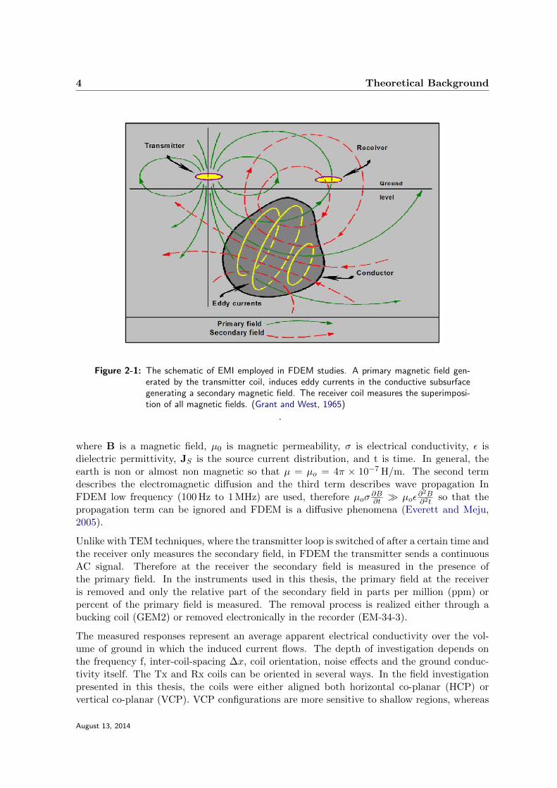
2-1 The schematic of EMI employed in FDEM studies. A primary magnetic field gen-erated by the transmitter coil, induces eddy currents in the conductive subsurfacegenerating a secondary magnetic field. The receiver coil measures the superimpo-sition of all magnetic fields. (Grant and West, 1965) . . . . . . . . . . . . . . . 4
2-2 Response function for EM-34-3 instrument coil configuration. For HCP the maxi-mum depth response is at greater depth with decreasing frequencies. In VCP themost sensitive part for all frequencies is at the surface. (Schultz and Ruppel, 2005) 5
2-3 Typical ranges of electrical resistivity [Ωm] for selected Earth materials (Reynolds,2011) . . . . . . . . . . . . . . . . . . . . . . . . . . . . . . . . . . . . . . . . . 6
2-4 Schematic illustration of a first year ridge, showing the sail and the keel (modifiedafter Timco and Burden (1997)) . . . . . . . . . . . . . . . . . . . . . . . . . . 7
3-1 A simplified flow chart of the inversion algorithm. . . . . . . . . . . . . . . . . . 17
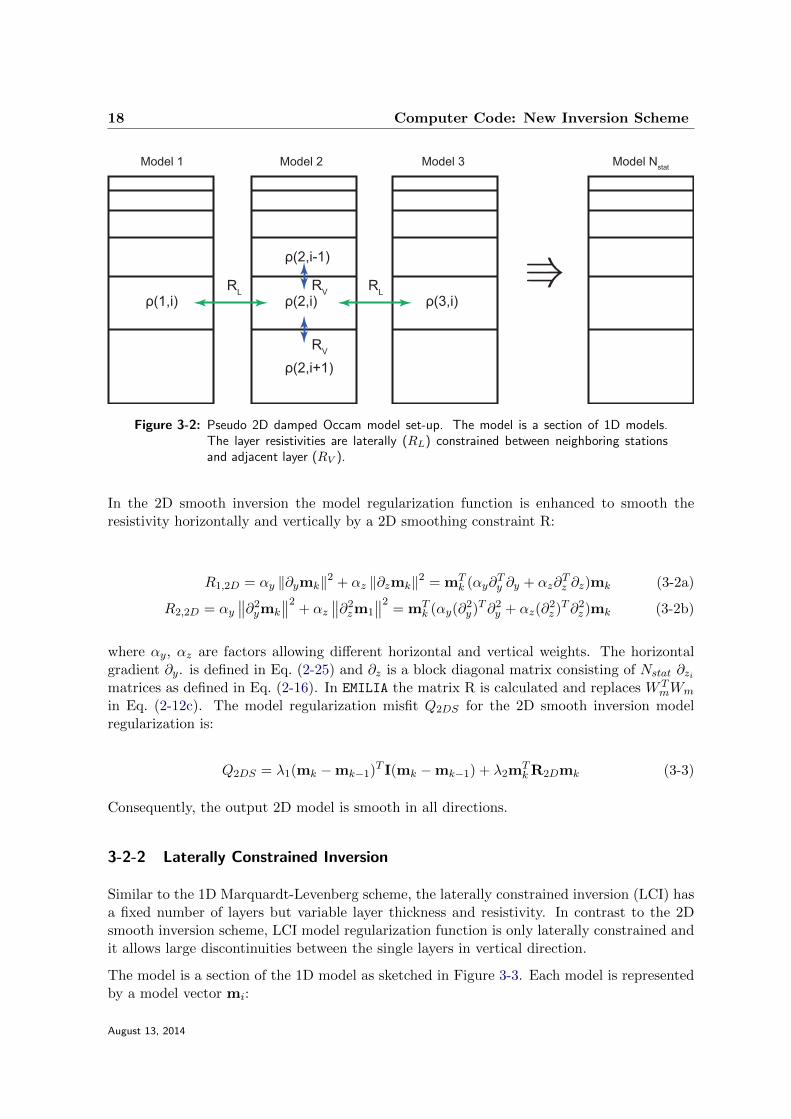
3-2 Pseudo 2D damped Occam model set-up. The model is a section of 1D models.The layer resistivities are laterally (RL) constrained between neighboring stationsand adjacent layer (RV ). . . . . . . . . . . . . . . . . . . . . . . . . . . . . . . 18
3-3 Laterally constrained inversion (LCI) model set-up. The model is a section of 1Dmodels. The layer thicknesses and resistivities are laterally constrained betweenneighboring stations. (modified after (Auken et al., 2005) . . . . . . . . . . . . 19
4-1 Geologial map of the survey area indicating the measured lines. . . . . . . . . . . 24
4-2 EM-34-3 field layout with the 10 m inter-coil spacing in vertical-coplanar (VCP)mode. . . . . . . . . . . . . . . . . . . . . . . . . . . . . . . . . . . . . . . . . 25
4-3 Fluctuation of measured EM Data over time for a) 10 m offset b) 20 m offset c)40 m offset . . . . . . . . . . . . . . . . . . . . . . . . . . . . . . . . . . . . . . 26
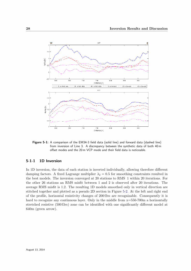
5-1 A comparison of the EM34-3 field data (solid line) and forward data (dashed line)from inversion of Line 3. A discrepancy between the synthetic data of both 40 moffset modes and the 20 m VCP mode and their field data is noticeable. . . . . 28
5-2 Line 2: Stitched 1D vertical smoothness constraint inversion with RMS misfits inthe bottom panel. The green arrow indicates the outlier in the resistive zone . . 29
August 13, 2014

xii List of Figures
5-3 Line 2: Pseudo 2D inversion with equal horizontal and vertical smoothness con-straint. RMS misfit in the bottom panel. The blue arrows indicates the lateralresistivity change disappearing with higher horizontal smoothing. The pink ellipsoidmark the conductive zone and . . . . . . . . . . . . . . . . . . . . . . . . . . . 29
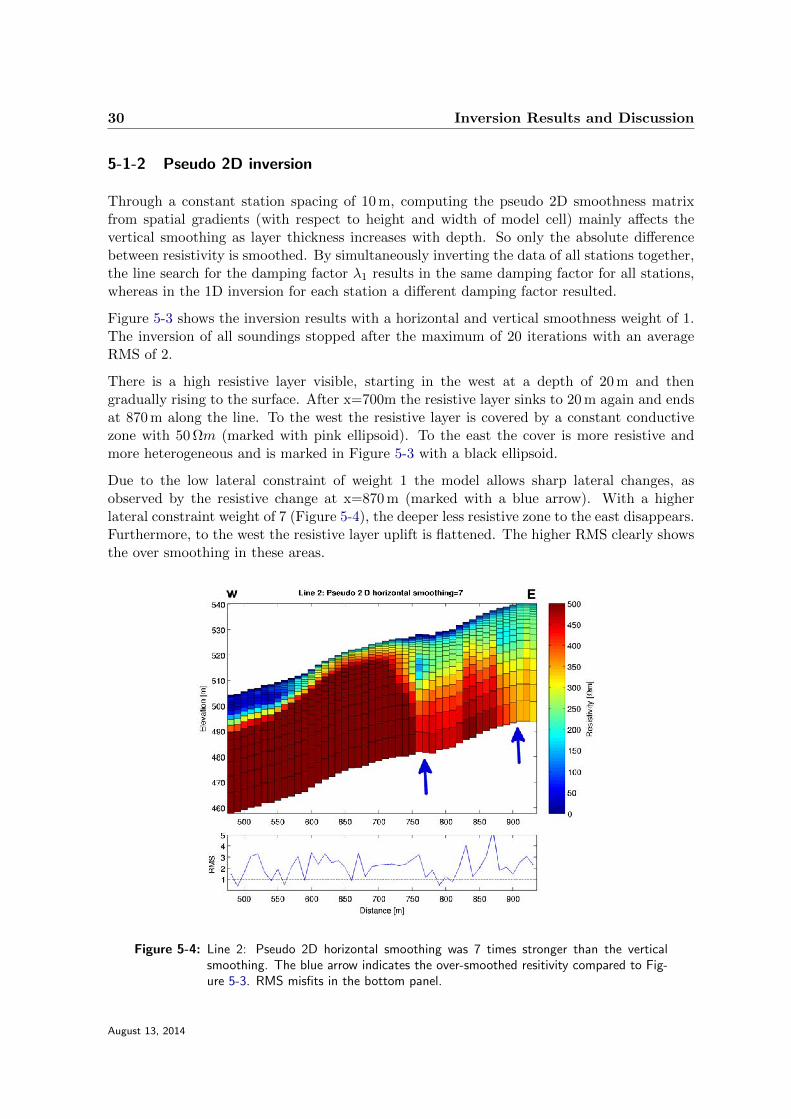
5-4 Line 2: Pseudo 2D horizontal smoothing was 7 times stronger than the verticalsmoothing. The blue arrow indicates the over-smoothed resitivity compared toFigure 5-3. RMS misfits in the bottom panel. . . . . . . . . . . . . . . . . . . . 30
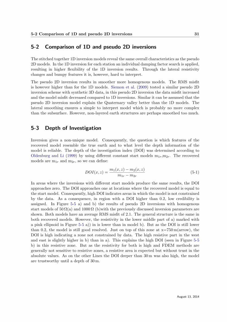
5-5 Resistivity models of line 2 generated with a constant start model of a) 50 Ω b)1000 Ω. Both models were inverted with the same parameters and show a similarRMS of around 2.1. The pink ellipsoid indicates the zone with the most visibleresistivity changes. In c) the depth of the investigation index (DOI) of the givenmodels is shown. . . . . . . . . . . . . . . . . . . . . . . . . . . . . . . . . . . . 32
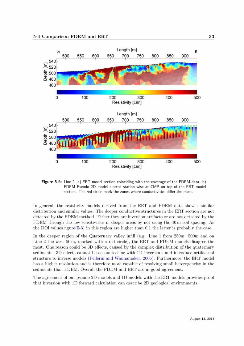
5-6 Line 2: a) ERT model section coinciding with the coverage of the FDEM data. b)FDEM Pseudo 2D model plotted station wise at CMP on top of the ERT modelsection. The red circle mark the zones where conductivities differ the most. . . 33
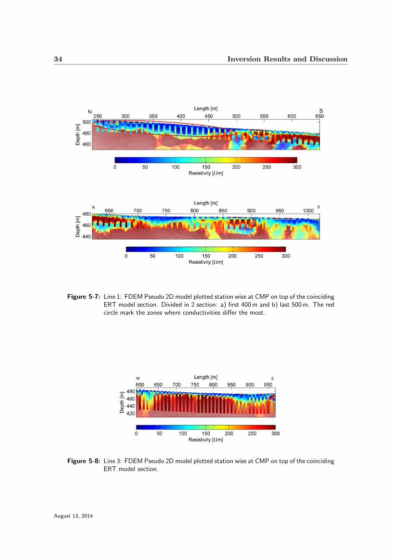
5-7 Line 1: FDEM Pseudo 2D model plotted station wise at CMP on top of thecoinciding ERT model section. Divided in 2 section: a) first 400 m and b) last500 m. The red circle mark the zones where conductivities differ the most. . . . 34
5-8 Line 3: FDEM Pseudo 2D model plotted station wise at CMP on top of thecoinciding ERT model section. . . . . . . . . . . . . . . . . . . . . . . . . . . . 34
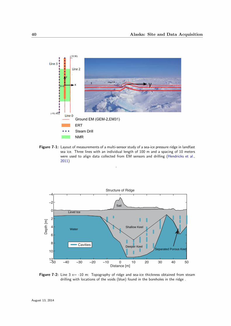
7-1 Layout of measurements of a multi-sensor study of a sea-ice pressure ridge inlandfast sea ice. Three lines with an individual length of 100 m and a spacing of10 meters were used to align data collected from EM sensors and drilling (Hendrickset al., 2011) . . . . . . . . . . . . . . . . . . . . . . . . . . . . . . . . . . . . . 40
7-2 Line 3 x= -10 m: Topography of ridge and sea-ice thickness obtained from steamdrilling with locations of the voids (blue) found in the boreholes in the ridge . . . 40
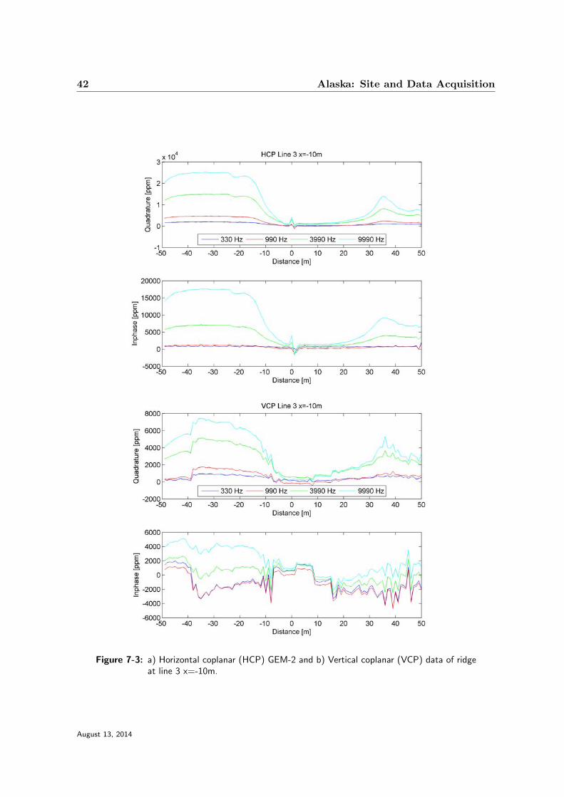
7-3 a) Horizontal coplanar (HCP) GEM-2 and b) Vertical coplanar (VCP) data of ridgeat line 3 x=-10m. . . . . . . . . . . . . . . . . . . . . . . . . . . . . . . . . . . 42
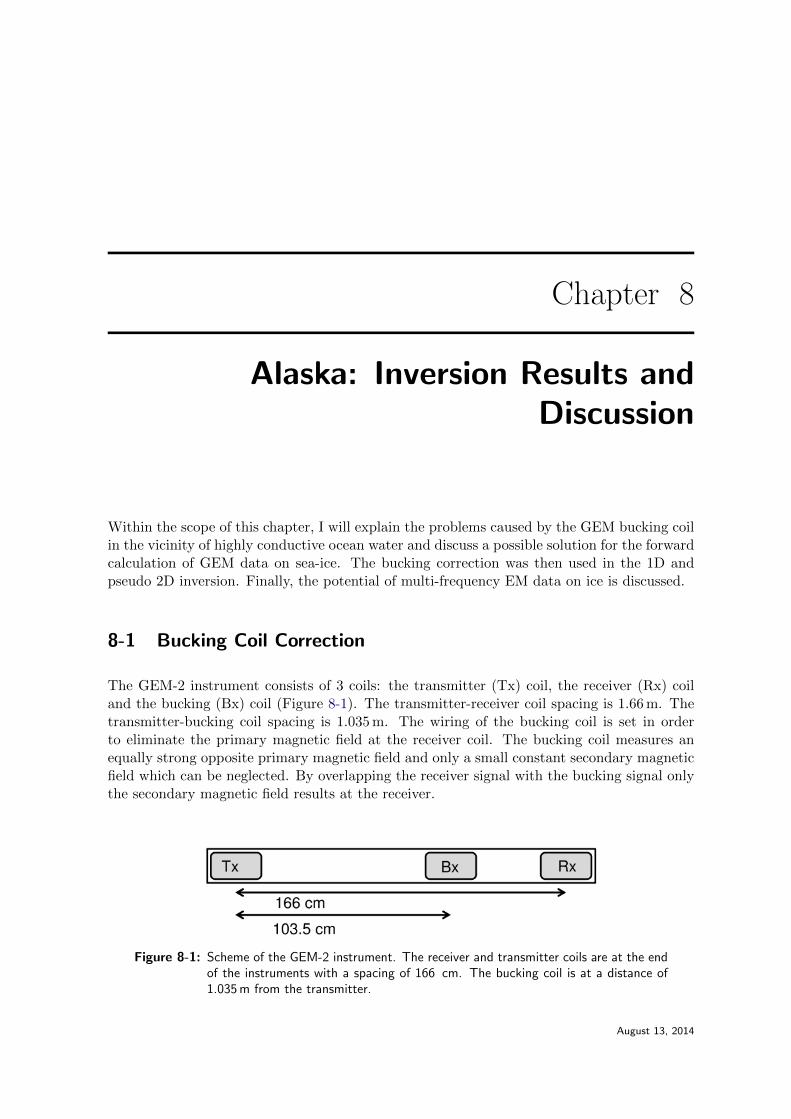
8-1 Scheme of the GEM-2 instrument. The receiver and transmitter coils are at theend of the instruments with a spacing of 166 cm. The bucking coil is at a distanceof 1.035 m from the transmitter. . . . . . . . . . . . . . . . . . . . . . . . . . . 43
8-2 Comparison of measured EM responses and forward calculations at 1830 Hz foran ice layer of 10 mS/m over a conductive half space of 2708 mS/m measured atdifferent heights above the ice. The stars represent the GEM field data. The linesare the forward calculations, in magenta FTx−Rx and in blue FTx−Bx . The redline is the resulting response Fres by subtraction FTx−Rx and FTx−Bx. . . . . . 45
8-3 Semi-analytical sensitivities for the resistivity of the ice layer for 18830 Hz normal(magenta), bucking coil (blue) and with the implemented bucking corrections inblack. The semi-analytical sensitivities are compared to the sensitivities from theperturbation approach. . . . . . . . . . . . . . . . . . . . . . . . . . . . . . . . 45
8-4 Line 3: Stitched 1D inversions vertical smoothness constraint; RMS misfits in thebottom panel. The pink boxes indicates zone with low sensitivities. . . . . . . . . 46
8-5 Three different start models a) 2-layer model with interface at 2 m and upper-layerresistivity of 100 Ωm and 0.4 Ωm for the confining half-space b) 3-layer model:first layer resistivity of 100 Ωm and thickness of 2 m, second layer resistivity of20 Ωm and thickness of 3 m and a half-space of 0.4 Ωm c) laterally varying 2-layerstart model, interfaces correlate roughly with drill depths, same resistivities as a). 47
8-6 Line 3: 1D Marquardt-Levenberg inversions a) 2-layer models and b) 3-layer withRMS at the bottom. For better visualizations the GPS heights shown at the top. 48
August 13, 2014
List of Figures xiii
8-7 Line 3: Laterally constrained inversion for a) 2-layer models and b) 3-layer modelsand c) with the laterally varying 2-layer start model. For better visualizations theGPS heights are shown on top. RMS misfits are shown in the bottom pannel. . . 50
8-8 Line 3: Laterally constrained inversion models with ice thickness and cavities assecond data sets. RMS misfits in the bottom panel. . . . . . . . . . . . . . . . . 51
8-9 Line 3: Laterally constrained inversion with single frequency of 9990 Hz data withRMS misfit in the bottom panel and topography at the top. . . . . . . . . . . . 53
8-10 Line 3: 2-layer inversion model from Figure 8-7 c) plotted with GPS height. . . . 54
8-11 Comparison of the model interface with ridge structure obtained from drilling . . 55
B-1 Line 1: Stitched 1D vertical smoothness constraint inversion with RMS misfits in 67
B-2 Line 1: Pseudo 2D horizontal and vertical smoothness constraint inversion with RMS 68
B-3 Line 3: Stitched 1D vertical smoothness constraint inversion with RMS misfits in 69
B-4 Line 3: Pseudo 2D horizontal and vertical smoothness constraint inversion with RMS 69
B-5 Line 1: Measured field data, HCP in top panel and VCP in the bottom panel. . . 70
B-6 Line 2: Measured field data, HCP in top panel and VCP in the bottom panel. . 71
B-7 Line 3: Measured field data, HCP in top panel and VCP in the bottom panel. . . 72
C-1 Line 0: Stitched 1D inversions vertical smoothness constraint; RMS misfits in the 73
C-2 Line 0: 1D Marquardt-Levenberg inversions a) 2-layer models and b) 3-layer withRMS at the bottom. For better visualizations the GPS heights shown at the top. 74
C-3 Line 0: Laterally constrained inversion for a) 2-layer models and b) 3-layer modelsand c) with the laterally varying 2-layer start model. For better visualizations theGPS heights are shown on top. RMS misfits are shown in the bottom panel. . . . 75
C-4 Line 2:1D Marquardt-Levenberg inversions a) 2-layer models and b) 3-layer withRMS at the bottom. For better visualizations the GPS heights shown at the top 76
C-5 Line 2:Laterally constrained inversion for a) 2-layer models and b) 3-layer modelsand c) with the laterally varying 2-layer start model. For better visualizations theGPS heights are shown on top. RMS misfits are shown in the bottom panel. . . . 77
C-6 a) Horizontal coplanar (HCP) GEM-2 and b) Vertical coplanar (VCP) data of ridgeat line 0 x=0m. . . . . . . . . . . . . . . . . . . . . . . . . . . . . . . . . . . . 78
C-7 a) Horizontal coplanar (HCP) GEM-2 and b) Vertical coplanar (VCP) data of ridgeat line 1 x=10m. . . . . . . . . . . . . . . . . . . . . . . . . . . . . . . . . . . 79
C-8 a) Horizontal coplanar (HCP) GEM-2 and b) Vertical coplanar (VCP) data of ridgeat line 3 x=-10m . . . . . . . . . . . . . . . . . . . . . . . . . . . . . . . . . . 80
August 13, 2014

xiv List of Figures
August 13, 2014
Acronyms
AWI Alfred Wegener Institute for Polar and Marine Research
CARNEVAL Characterization And Removal of Near-surface Effects of Value for Applica-tions in Land seismics
CMP Common midpoint
DOI Depth of Investigation
DUT Delft University of Technology
EMILIA ElectroMagnetic Inversion with Least Intricate Algorithms
EM Electromagnetic
EMI Electromagnetic Induction
ERT Electrical Resistivity Tomography
ETH Swiss Federal Institute of Technology
FDEM Frequency domain electromagnetic
GPS Global Positioning System
HCP horizontal co-planar
LCI Laterally constrain inversion
LINA low induction number approximation
RMS Root-Mean-Square
RWTH Aachen University
Rx Receiver
August 13, 2014

xvi Acronyms
SNMR Surface Nuclear Magnetic Resonance
TEM Time-domain electromagnetic
Tx Transmitter
VCP vertical co-planar
August 13, 2014
Chapter 1
Introduction
Electromagnetic (EM) sounding is a widely used method for near subsurface exploration.It is for instance applied to solve environmental and hydro geophysical surveying problemsor to measure the thickness of sea-ice. Basically, electromagnetic fields actively inducedin electrically conductive ground are measured at the surface to determine the subsurfaceconductivity distribution through an inversion process. A fast way to map the lateral andvertical conductivity distribution is the frequency domain electromagnetic method (FDEM).Commonly the data are inverted 1D at each single station (=measurement location) into asmooth earth model (Occam inversion, Oldenburg and Li (1999)) or into a model with sharplayer interfaces (Marquardt Levenberg scheme Lines and Treitel (1984)). In a typical layeredsituation (e.g. sedimentary layers or ice layers) the resistivity varies horizontally less thanvertically and as a consequence, constraining the inversion laterally amongst neighboringstations should improve the inversion results.
To related layered models from abutting sounding locations, different lateral constraint in-version techniques have been developed so far. Since forward responses and sensitivities arecomputed for a 1D model section underneath each station. All of these techniques can beconsidered pseudo 2D inversions. One approach is to simultaneously invert all collected data1D, but with vertical and horizontal smoothing constraints. Naturally, the resulting 2D earthconductivity models are less blocky than 2D earth models resulting from the concatenation ofindependent 1D inversion results (Schultz and Ruppel, 2005; Monteiro Santos, 2004). Anothertechnique is the laterally constrained inversion (LCI) by Christiansen and Auken (2004). Theoutput is a laterally smooth 2D model with sharp layer interfaces in the vertical direction.
In the framework of this thesis, pseudo 2D inversions with 2D smoothness and LCI wereimplemented in the existing inversion program EMILIA for ElectroMagnetic Inversion withLeast Intricate Algorithms (Kalscheuer, 2014). EMILIA is an object-oriented inversion programwritten in Fortran 2008, able to invert different kinds of electromagnetic data. The enhancedcode was tested on two different field data. First, on data acquired with a Geonics EM-34-3instrument1 in a valley filled with Quaternary sediments. Second, on a data set collected
1 FDEM instrument with Tx-Rx coil spacings of 10, 20 and 40 m more informationhttp://www.geomatrix.co.uk
August 13, 2014

2 Introduction
across sea ice pressure ridge with a GEM-2 system 2.
Quaternary sediments are highly heterogeneous and lead to distortion in geophysical survey-ing (Schmelzbach et al., 2014).The survey of the quaternary sediments took place within theCARNEVAL (=Characterization And Removal of Near-surface Effects of Value for Applica-tions in Land seismics) project of ETH. It aims, among other things, on the establishment ofa near surface model of the Quaternary valley in northern Switzerland. A multi-method geo-physical campaign including seismic reflection/refraction surveys, multi-component seismic,geoelectric (ERT) and TEM measurements was carried out. The FDEM data supplementsthe near surface model of the valley.
Normally sea-ice is considered as a homogeneous layer representing a simple 2 layer 1D case,namely a resistive ice layer on top of the ocean water considered a conductive half space.However, pressure ridges consist of crashed, broken-up and piled sea-ice blocks [e.g (Pfafflinget al., 2007)]. 1D inversion often fails to sufficiently explain these 3D structures which resultsin an underestimation of the sea ice thickness. Using the GEM-2 instrument on highlyconductive ground such as saline ocean water introduces an additional problem; an inductivefeedback between ocean water and bucking coil. This feedback signal is not considered in theforward calculation within EMILIA. In this thesis I will introduce a present correction of thisfeedback problem in the calculation of forward responses and sensitivities. Recent discussionsin the sea-ice research community address the potential of multi frequency EM to determineinternal sea-ice structures (Pfaffling et al., 2007; Hunkeler et al., 2015) . Therefore, in thisthesis I examine the sensitivity of the inversion result to the used frequency ranges.
1-1 Thesis Objectives and Outline
The overall aim of this thesis is to test if pseudo 2D inversion of FDEM data results in morerealistic models than 1D inversion. The new inversion scheme will be compared to frequentlyused 1D inversion schemes such as damped Occam and Marquart-Levenberg inversions intwo separate field studies. Another goal is to see if FDEM can be used to resolve complexstructures like Quaternary sediments or sea-ice pressure ridges.
The thesis is divided into four main parts. First I will provide an overview of the relevanttheory of FDEM and 1D modeling. Next, the two pseudo 2D inversion schemes are explained.Then the field study sites are introduced. For both of them survey parameters, data and 1Dand pseudo 2D inversion results are described followed by a small discussion. At last, anoverall conclusion is drawn and an outlook for further work is given.
2 FDEM instrument with fixed coil spacings of 1.66 m and variable multy-frequency in the range of 330 Hzto 24 kHz more information http://terraplus.ca/
August 13, 2014

Chapter 2
Theoretical Background
In this chapter the theoretical background for the coil-coil frequency domain electromagnetic(FDEM) is briefly explained together with an overview of the geoelectrical properties of buriedvalleys and ice.
2-1 Frequency Domain Electromagnetic
Electromagnetic induction (EMI) is based on the interaction between actively created EMfields and a conductive subsurface. The frequency domain electromagnetic method (FDEM)is an active EM method with a controlled source. This chapter describes the basic conceptof FDEM in a very brief way, for further information refer to standard EM textbooks (e.g.Frischknecht et al., 2001; Reynolds, 2011).
The schematic of EMI with the FDEM method is shown in Figure 2-1. The basic instru-ment consists of two coils. A transmitter (Tx) coil is energized by an alternating current Jat a fixed frequency generating a primary magnetic field HP. The primary magnetic fieldinduces circular eddy currents in conducting materials according to Faraday’s law. The cur-rent strength depends on the resistance and inductance of the subsurface. The eddy currentsproduce a secondary magnetic field HS according to Amperes law containing the subsurfaceinformation. The primary plus secondary magnetic field are measured at the receiver coil(Rx) as an induced AC voltage with amplitude and phase shifted relative to the primaryfield. The secondary field is a complex-value quantity with the real part called in-phase andthe complex part called quadrature.
EM induction methods work in a quasi static environment. This means for the low frequenciesranges of small coil FDEM systems any magnetic field generated by displacement current isnegligible and the magnetic field is described by steady electrical currents. Considering allfour Maxwell equations the wave equation for EM waves can be derived (Everett and Meju,2005):
∇2B − µoσ∂B
∂t− µoε
∂2B
∂2t= µo∇× J (2-1)
August 13, 2014
4 Theoretical Background
Figure 2-1: The schematic of EMI employed in FDEM studies. A primary magnetic field gen-erated by the transmitter coil, induces eddy currents in the conductive subsurfacegenerating a secondary magnetic field. The receiver coil measures the superimposi-tion of all magnetic fields. (Grant and West, 1965)
.
where B is a magnetic field, µ0 is magnetic permeability, σ is electrical conductivity, ε isdielectric permittivity, JS is the source current distribution, and t is time. In general, theearth is non or almost non magnetic so that µ = µo = 4π × 10−7 H/m. The second termdescribes the electromagnetic diffusion and the third term describes wave propagation InFDEM low frequency (100 Hz to 1 MHz) are used, therefore µoσ
∂B∂t µoε
∂2B∂2t
so that thepropagation term can be ignored and FDEM is a diffusive phenomena (Everett and Meju,2005).
Unlike with TEM techniques, where the transmitter loop is switched of after a certain time andthe receiver only measures the secondary field, in FDEM the transmitter sends a continuousAC signal. Therefore at the receiver the secondary field is measured in the presence ofthe primary field. In the instruments used in this thesis, the primary field at the receiveris removed and only the relative part of the secondary field in parts per million (ppm) orpercent of the primary field is measured. The removal process is realized either through abucking coil (GEM2) or removed electronically in the recorder (EM-34-3).
The measured responses represent an average apparent electrical conductivity over the vol-ume of ground in which the induced current flows. The depth of investigation depends onthe frequency f, inter-coil-spacing ∆x, coil orientation, noise effects and the ground conduc-tivity itself. The Tx and Rx coils can be oriented in several ways. In the field investigationpresented in this thesis, the coils were either aligned both horizontal co-planar (HCP) orvertical co-planar (VCP). VCP configurations are more sensitive to shallow regions, whereas
August 13, 2014
2-1 Frequency Domain Electromagnetic 5
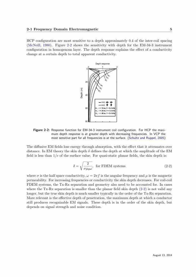
HCP configuration are most sensitive to a depth approximately 0.4 of the inter-coil spacing(McNeill, 1980). Figure 2-2 shows the sensitivity with depth for the EM-34-3 instrumentconfiguration in homogenous layer. The depth response explains the effect of a conductivitychange at a certain depth to total apparent conductivity.
Figure 2-2: Response function for EM-34-3 instrument coil configuration. For HCP the maxi-mum depth response is at greater depth with decreasing frequencies. In VCP themost sensitive part for all frequencies is at the surface. (Schultz and Ruppel, 2005)
The diffusive EM fields lose energy through absorption, with the effect that it attenuates overdistance. In EM theory the skin depth δ defines the depth at which the amplitude of the EMfield is less than 1/e of the surface value. For quasi-static planar fields, the skin depth is:
δ =
√2
σµ0ω, for FDEM systems (2-2)
where σ is the half space conductivity, ω = 2πf is the angular frequency and µ is the magneticpermeability. For increasing frequencies or conductivity the skin depth decreases. For coil-coilFDEM systems, the Tx-Rx separation and geometry also need to be accounted for. In caseswhere the Tx-Rx separation is smaller than the planar field skin depth (2-2) is not valid anylonger, but the true skin depth is much smaller typically in the order of the Tx-Rx separation.More relevant is the effective depth of penetration, the maximum depth at which a conductorstill produces recognizable EM signals. These depth is in the order of the skin depth, butdepends on signal strength and noise condition.
August 13, 2014
6 Theoretical Background
2-2 Electrical Properties of Earth Materials
2-2-1 Quaternary Sediments
The conductivity of the subsurface holds information about the mineralogy, texture and watercontent. The conductivity of shallow sediments like Quaternary sediments is mostly controlledby the porosity and water and clay content. The magnitude of the total conductivity σ isa combination of electrolytic conduction (Archies law) and surface conduction due to clayminerals (Reynolds, 2011):
σ = aφmSnσf + σs (2-3)
with bulk conductivity σ (S/m), proportionality factor a, fractional porosity φ of intercon-nected pore space, cementation exponent m, fraction S of pores containing water, saturationconstant n, pore fluid conductivity σf , and surface conductivity σs.
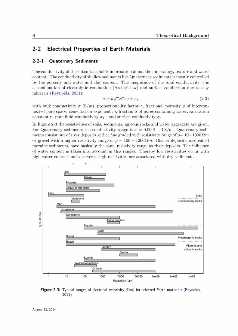
In Figure 2-3 the resistivities of soils, sediments, igneous rocks and water aggregate are given.For Quaternary sediments the conductivity range is σ = 0.0001 − 1 S/m. Quaternary sedi-ments consist out of river deposits, either fine graded with resistivity range of ρ= 10−1000 Ωmor gravel with a higher resistivity range of ρ = 100 − 1200 Ωm. Glacier deposits, also calledmoraine sediments, have basically the same resistivity range as river deposits. The influenceof water content is taken into account in this ranges. Thereby low resistivities occur withhigh water content and vice versa high resitivities are associated with dry sediments.
Figure 2-3: Typical ranges of electrical resistivity [Ωm] for selected Earth materials (Reynolds,2011)
August 13, 2014
2-2 Electrical Properties of Earth Materials 7
2-2-2 Sea-ice and ocean
The conductivity of the ocean water depends on the water temperature and salinity. Thewater temperature below ice is close to the freezing point, resulting in a conductivity of 0.3S/m in the Baltic sea and up to 2.4 S/m in the Arctic or Antarctica. In general, the sea-iceconductivity is two magnitudes smaller than the conductivity of the water from which it wasformed and it is between 1 mS/m (Baltic) and 50 mS/m (Arctic). As a result of the sharpcontrast between ice and seawater the induced eddy currents flow mostly in sea water (Pfafflinget al., 2007). Sea ice imparts a strong conductivity anisotropy to the sea ice, with the bulkconductivity in the vertical direction being higher than that in the horizontal direction. Theskin depth((2-2)) depends on the conductivity. In ice with low conductivity the EM signal ishardly attenuated, for example a sounding with 9990 Hz in the Arctic ice(50 mS/m) the skindepth is approximate 22 m. In the conductive water the skin depth is with approximate 3 msmall.
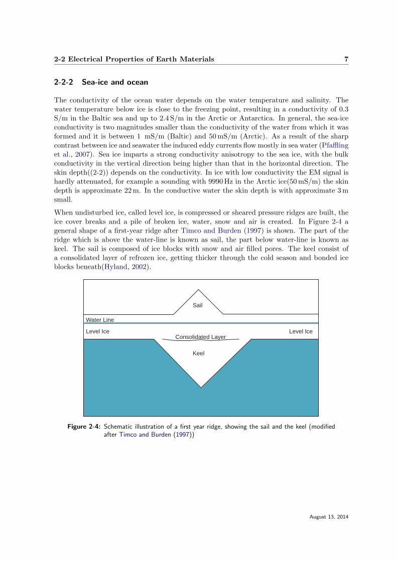
When undisturbed ice, called level ice, is compressed or sheared pressure ridges are built, theice cover breaks and a pile of broken ice, water, snow and air is created. In Figure 2-4 ageneral shape of a first-year ridge after Timco and Burden (1997) is shown. The part of theridge which is above the water-line is known as sail, the part below water-line is known askeel. The sail is composed of ice blocks with snow and air filled pores. The keel consist ofa consolidated layer of refrozen ice, getting thicker through the cold season and bonded iceblocks beneath(Hyland, 2002).
Sail
Keel
Water Line
Level Ice Level IceConsolidated Layer
Figure 2-4: Schematic illustration of a first year ridge, showing the sail and the keel (modifiedafter Timco and Burden (1997))
August 13, 2014
8 Theoretical Background
2-3 Inversion Theory
Inversion is the process of finding a model describing the measured data the best , i.e. whereforward calculated data and measured data have a minimal misfit. This can be done withdifferent algorithms. Only a basic introduction is provided in this thesis. An overview aboutinversion methods and theory can be found e.g. in Lines and Treitel (1984); Menke (2012).
The iterative process of finding the subsurface model describing the data best involves twomain parts: 1. Forward modeling and creation of synthetic data 2. The inversion algorithmitself, changing the subsurface model in order to reduce the misfit between synthetic andmeasured data.
Forward modeling computes the synthetic response of a model stored in vector dfwd containingN data points. The subsurface is defined by model parameters which are stored in the modelvector m of length M. The relation from the model to forward data is described by themathematical function F:
dfwd = F[m] (2-4)
It is assumed that the measured data dobs represent the response of the true model and datauncertainties. The inversion scheme changes the model parameters so that the misfit betweenmodel response and the measured measured data dobs is minimal. Normally, this is done witha least squares-technique, involving an l2 norm which is the square of all data misfit. Thedata misfit objective function Qd to minimize is described by Lines and Treitel (1984)
Qd =∥∥∥Wdd
obs −WdF[m]∥∥∥2,with Wd =
1σ1
. . . 0... 1
σ2
......
. . .
0 . . . 1σN
(2-5)
By using the data weighting matrix Wd with the inverse of the uncertainties σd,i the solutionis controlled by data points with small uncertainties. To obtain an arithmetic misfit valuethe sum of the squares of the derivation between field data and forward response scaled bythe data error σi normed by the number of data N points and the square root taken referringto as root-mean-square error (RMS).
RMS =
√√√√ 1
N
N∑i=1
diobs − Fiσi
(2-6)
Assuming a linear relation between data and model parameter, F[m] can be replaced by theproduct of the data kernel matrix G with the model vector m. As a consequence, the generallinear discrete inverse problem is described as:
m = G−gdobs (2-7)
When G is square (N = M) and regular G−g is the inverse of the data kernel matrix. How-ever, in most cases G−g is a more complicated combination of mathematical relationships
August 13, 2014
2-3 Inversion Theory 9
involving the transpose GT and matrix multiplications. For overdetermined inverse problem,the equation is solved with the least square-technique. Therefore, Eq. (2-7) is rewritten forover-determined problems as:
m = (GTG)−1GTdobs (2-8)
Since most geophysical problems are non-linear and underdetermined, Eq. (2-4) is linearizedwith a first order of Taylor expansion around a reference model m0
F[m] = F[m0] +∂F[m0]
∂m(m1 −m0) + e (2-9)
with e being the error of the higher order Taylor series approximations. The partial derivativesare also called the sensitivities of a specific model parameter and describe the change of eachcomponent of dfwd due to a small modification of model parameters in m0. The derivativesof the forward problem with respect to model parameters can be written as a Jacobian matrixJ of size N x M. Each component is defined as:
Jij =∂Fi[m0]
∂mji = 1, ..., N j = 1, ..., N (2-10)
By inserting the Jacobian matrix into Eq. (2-9), the forward equation is
F[m] = F[mk] + J∆m (2-11)
Since the Taylor expansion is only used as a first order expansion, repetitive approximationis required to find the minimum of the misfit function. Hence, ∆m is the difference of themodel of the current iteration k and previous iteration k-1., i.e ∆m = mk−mk−1. The modelis updated each time with an optimization algorithm. The resulting model of one inversioniteration is used as start model mk−1 for the following iteration to find a improved mk. Theprocedure is repeated until the misfit is smaller than the target misfit (Q∗
d) or a maximum ofiterations is reached.
However, most of the inversion problems are under or mixed determined, so by only usingthe misfit, the inversion will lead to a diverging solution with implausible model parameters.Consequently to stabilize the inversion, regularization has to be considered.
The combination of data misfit Qd (Eq. (2-5)) and model regularization Qm is written in thecost function (Menke, 2012):
U [m, λ] = (Qd[m]−Q∗d) + λQm[m] (2-12a)
with
Qd[m] = (d− F[m])TWTd Wd(d− F[m]) (2-12b)
Qm[m] = (m−mr)TWT
mWm(m−mr) (2-12c)
August 13, 2014
10 Theoretical Background
The Lagrange multiplier λ describes the weight of the additional model constraint relativeto the constraint provided by the data. The model regularization matrix Wm describes thesimplicity between the models.
Different inversion schemes exist. In the following section, I describe the schemes used in mythesis.
2-3-1 Marquardt-Levenberg Inversion
In the Marquardt-Levenberg-method, the data misfit is combined with damping constraintswhere the difference between the new model mk and the previous model mk−1 is limited. Inthe l2 norm, Lines and Treitel (1984) introduced the damping constraint as
Qdamp = λ1 ‖mk −mk−1‖2 (2-13)
where λ1 is a Lagrange multiplier controlling the magnitude of the damping. A high λ1
indicates high confidence in the previous model m0. Accordingly, the model regularizationmatrix in Eq. (2-12c) is an identity matrix Wm = I. The resulting cost function UMarq =Qd +Qdamp depends on the start model. Resistivities and thicknesses of the layers are modelparameters and modified during the inversion. Therefore, large discontinuities between thelayer resistivities are admissible.
2-3-2 Occam
Because of the non-unique behavior of inversion solutions, the simplest and thereforesmoothest model is sought in a n Ocam inversion. This guarantees that the real earth isat least as rich in structure as the model (Constable et al., 1987). For this purpose the Earthis discretized into M layers of fixed thickness that increases logarithmically equidistantly fromthe shallowest layer towards greater depth with a factor of e.g. 1.2 or 1.3, where l=1,..M.Only the layer resistivities are allowed to vary during the inversion; and it is the resistivitiesonto which smoothness constraints are imposed.
Vertical smoothing
The smoothing constrains the structural features, by minimizing the difference between spa-tially adjacent model parameters. For the resistivities of the l-th and (l+1)-th layer, firstorder smoothness constraints take the form:
ρl − ρl+1
∆zl≈ 0→ ∂zρ ≈ 0 (2-14)
Therefore, the smoothing is defined with ∂z the vertical gradient.
The roughness matrix R replacing WTmWm from Eq. (2-12c) contains the first or second
order derivatives of the model parameters m with respect to depth, defined by (Constableet al., 1987) as:
R1,z = ‖∂zm‖2 = mT∂Tz ∂zm (2-15a)
R2,z = ‖∂z∂zm‖2 =∥∥∂2
zm∥∥2
(2-15b)
August 13, 2014
2-3 Inversion Theory 11
In a 1D model with Nlay layers, ∂z is square a matrix of size M ×M :
∂z =
−1∆z1
1∆z2
. . . 0
−1∆z2
1∆z3
...
0 0...
. . .
. . . −1∆zNlay−1
1∆zNlay
0 . . . 0
(2-16)
and the second-order difference matrix ∂2z :
∂2z =
0 . . . 01
∆z1−2∆z2
1∆z2
0 0
0 1∆z2
−2∆z3
1∆z3
0...
.... . .
0 1∆zNlay−2
−2∆zNlay−1
1∆zNlay
0 . . . 0
(2-17)
where ∆zi is the layer thickness.
In the l2 norm, the 1D vertical smoothing for constraint Qsmooth becomes:
Qsmooth = λ2 ‖WSm‖2 ,with WS = ∂zor WS = ∂2z (2-18)
where λ2 is the balance between the data misfit and the smoothing constraint. The costfunction to minimize is UOccam = Qd + Qsmooth and is solved for the desired smooth modelwithin the error tolerance.
2-3-3 Damped Occam
The third scheme in this thesis, used for the Quaternary sediments, is a Marquardt-Levenbergdamped Occam inversion (Kalscheuer et al., 2012). The inversion scheme uses additionallyto smoothness constraints Qsmooth Marquardt-Levenberg damping Qdamp . The cost functionof the damped Occam inversion becomes then UDamocc = Qd +Qdamp +Qsmooth:
UDamocc =∥∥∥Wdd
obs −WdF[m]∥∥∥2
+ λ1 ‖mk −mk−1r‖2 + λ2 ‖WS(mk −mr)‖2 (2-19)
or
UDamocc = (d− F[mk])TWT
d Wd(d− F[mk]) + λ1(mk −mk−1)T I(mk −mk−1)
+λ2(mk −mr)∂Tz ∂z(mk −mr) (2-20a)
August 13, 2014

12 Theoretical Background
Where mr is a reference model that represents a preferred solution. Substitution of the first-order Taylor series of the forward operator in Eq. (2-11) into Eq. (2-19)yields a cost functionalquadratic in mk.
UDamocc =∥∥Wd(d
obs − F[mk−1] + Jmk−1 − Jmk)∥∥2
+ λ1 ‖mk −mk−1‖2
+λ2 ‖WSmk−1 −mr‖2 (2-21a)
The new model is found by minimizing the cost function UDamocc, by setting ∇mU = 0 andsolving the resulting equation for mk.
m1λ = [JTWTd WdJ + λ1I + λ2R]−1((JWd)
TWd + λ1(mk−1))d + mr (2-22)
where d = dobs − F[mk−1] + J(mk −mk−1) is a modified data difference vector.
2-3-4 Pseudo 2D
Layered earth 1D inversion assumes horizontal layers with only slow lateral resistivity changes.Since field data hold information from more dimensions, interpretation of 1D models can bemisleading. Furthermore in FDEM methods, the lateral sensitivity of the instrument partlyoverlaps when the models of inter coil spacing are about the size of or larger than the linespacing. Consequently, a model being algorithmically constraint by models of neighboringstations is essential. The so called pseudo 2D inversion is a parameterized inversion of dataof the same type with lateral constraints on the model parameters between neighboring pa-rameters.
The output model is controlled by the field data, the constraints to the model of the neigh-boring stations and the inversion method. Model parameters with low sensitivity are mainlycontrolled by the constraint. The lateral constraint can be considered as priori informationof the geological variability. Depending on lateral variance of the subsurface, the constrainthas to be chosen smaller or bigger (Auken and Christiansen, 2004).
In pseudo 2D inversion (Christiansen and Auken, 2004; Schultz and Ruppel, 2005), all datasets of all stations nstat are inverted simultaneous (for layered 1D models) minimizing acommon objective function lateral constrain in the model regularization function. At eachstation ns data constraints are complemented with data constraints from neighboring stationswhich may have different depth sensitivities and thus lead to a better constrained model. Allmeasurements along the profile are assembled in the field data vector dobs. A profile has Nstat
measurements points (=number of stations) yi where i = 1, Nstat. The pseudo 2D modelconsist of Nstat stitched together 1D models with each having Nlay.
Lateral Constraint
Similar to the vertical smoothing (section 2-3-2), the lateral constraints implemented in pseudo2D Occam inversion consist of minimizing adjacent model parameters in lateral direction. Thelateral constraint is defined through the horizontal partial derivative ∂y:
August 13, 2014

2-3 Inversion Theory 13
∂y =
∂y1 . . . 0
0 ∂y2...
∂y3...
.... . .
0 ∂yNstat
=
∂y1 . . . 0
0 ∂y2...
. . ....
... ∂yNstat−1
0 0
(2-23)
where ∂yi and 0 are blocks matrices of size Nlay × 2Nlay:
∂yi =
−1∆yi
0 0
0 −1∆yi
......
. . .
0 . . . −1∆yi︸ ︷︷ ︸
yi
1∆yi+1
0 0
0 1∆yi+1
......
. . .
0 . . . 1∆yi+1︸ ︷︷ ︸
yi+1
(2-24)
as recognizable the matrix (2-24) consists of two parts: yi for the constraints provided bystation i and yi+1 for the adjacent station. The offset between the the entries of yi andyi+1 represent the offset in memory order with which the layer parameters of the individualstations are stored in memory. Therefore, ∂y can be rewritten as:
∂y =
−∂y1 ∂y2 . . . 0
0 −∂y2 ∂y3...
.... . .
... −∂yNstat−1 ∂yNstat
0 0
,with ∂y =
1
∆yi0 0
0 1∆yi
0...
.... . .
0 . . . 1∆yi
(2-25)
Where ∂yi and 0 are square matrices of size Nlay×Nlay and where ∆yi is the spacing betweenstations. The dimension of the square matrix ∂y is Nlay ∗Nstat ×Nlay ∗Nstat.
It is also possible to design a second order difference matrix:
∂2y =
∂y1 −2∂y2 ∂y3 0
0 ∂y2 −2∂y3 ∂y4...
.... . .
... ∂yNstat−2 −2∂yNstat−1 ∂yNstat
0 0
(2-26)
where ∂yi and 0 are square matrices of size Nlay × Nlay. In this case the -2 corresponds tothe constraints provided by station yi and the 1 the adjacent stations to the left (yi−1) andright (yi+1).
August 13, 2014

14 Theoretical Background
For the LCI scheme originally presented by Christiansen and Auken (2004) the lateral differdifferencing of layer resistivities and thickness of layered models of abutting stations is similarto the one presented above for pseudo 2D Occam inversion with central differences in matrixsize and offset.
August 13, 2014

Chapter 3
Computer Code: New InversionScheme
In the framework of this chapter, I describe how the computer code was developed for laterallyconstraint inversions.
3-1 State of EMILIA
EMILIA for ElectroMagnetic Inversion with Least Intricate Algorithms (Kalscheuer, 2014) is asoftware package comprising object-oriented Fortran 2008 inversion code for electromagneticdata (Kalscheuer et al., 2010). Up to the commencement of my MSc thesis project thefrequency domain EM part was based on 1D models with the Occam, damped Occam andMarquardt-Levenberg inversion schemes described in section 2-3.
3-1-1 Forward Calculation
The 1D EM forward modeling routine from EMILIA is based on the assumption that conduc-tivities vary only with depth and are infinite in horizontal direction.
For controlled sources, the forward calculations are functions of radial spatial wave number, adistribution of which must be evaluated and integrated through a fast Hankel transformationto obtain the full spatial field or potential variation. For details please refer to Grab (2012)and Weidelt (1986).
3-1-2 1D EM Inversion
In EMILIA, 1D models for Occam and damped Occam inversions have fixed layer thickness.The thickness of each layer is iteratively increased by a constant factor of e.g. 1.2-1.4 withincreasing depth. The last layer is a confining half-space.
August 13, 2014

16 Computer Code: New Inversion Scheme
The iteration process of the damped Occam inversion contained in EMILIA performed in eachiteration a line search for the Lagrange multiplier λ1, which controls the damping constraint.To find the best λ1 in each iteration, for each detected λ1 the value of the data misfit Qd isdetermined and λ1 is varied with a certain step size within an user specified interval. Thesmoothness is controlled by the Lagrange multiplier λ2 which is directly specified by the user,and it is constant for all iterations.
3-2 Pseudo 2D Inversion
The algorithms for the pseudo 2D inversion are adopted from the existing 1D damped Occaminversion.
The flow chart in Figure 3-1 illustrates how the pseudo 2D inversion works. In a first step theprogram reads the input file, which provides the algorithm information about the number ofdata sets and the index of the data set. Each data set has an additional information file whereits station number and the maximum station number of the model are defined. Afterwards,the start model is read in either for all stations in the same way or individually defined foreach station. The model vector is initialized according to the free chosen model parametertypes. The 1D forward routine calculates synthetic data according to the model vector mi forall data sets individually. If the RMS is higher than 1, the laterally constrained cost functionis minimized including a line search for λ1 and an updated model is acquired. The processstarts with the forward calculation and the model is revised iteratively until the overall RMSis lower than 1 or a maximum number of iterations is reached.
For the pseudo 2D inversion, the vectors and matrices were enhanced to hold all stationssimultaneously.
In EMILIA the smoothness matrix is either scaled by the absolute differences corresponding to∆z = 1.and ∆y = 1 or by horizontal and vertical gradients of the cell resistivity (∆z=layerthickness and ∆y = Dy). The horizontal distance Dy between the models is computed ashalf the sum of the distances to the preceding and following stations.
3-2-1 2D Smooth Inversion
The pseudo 2Dsmooth inversion is based on the 1D damped Occam scheme. In this thesisreferred to as 2D smoothing inversion.
The models consist of 1D layered models mi with Nlay layers with fixed thickness as sketchedin Figure 3-2. The subsurface at station i as represented by a model vector mi consisting ofthe logarithmic resistivity for each layer:
mi = (log(ρi,1), log(ρi,2), ..., log(ρi,Nlay) (3-1)
The full model vector mT = (mT1 ,m
T2 , ...m
TNstat
) for all stations has a length of Nstat ×Nlay.
August 13, 2014

3-2 Pseudo 2D Inversion 17
Figure 3-1: A simplified flow chart of the inversion algorithm.
August 13, 2014
18 Computer Code: New Inversion Scheme
V
Model 1 Model 2 Model 3 Model Nstat
ρ(1,i) ρ(2,i)
ρ(2,i-1)
ρ(2,i+1)
ρ(3,i)R
LR
LR
V
RV
Figure 3-2: Pseudo 2D damped Occam model set-up. The model is a section of 1D models.The layer resistivities are laterally (RL) constrained between neighboring stationsand adjacent layer (RV ).
In the 2D smooth inversion the model regularization function is enhanced to smooth theresistivity horizontally and vertically by a 2D smoothing constraint R:
R1,2D = αy ‖∂ymk‖2 + αz ‖∂zmk‖2 = mTk (αy∂
Ty ∂y + αz∂
Tz ∂z)mk (3-2a)
R2,2D = αy∥∥∂2
ymk
∥∥2+ αz
∥∥∂2zm1
∥∥2= mT
k (αy(∂2y)T∂2
y + αz(∂2z )T∂2
z )mk (3-2b)
where αy, αz are factors allowing different horizontal and vertical weights. The horizontalgradient ∂y. is defined in Eq. (2-25) and ∂z is a block diagonal matrix consisting of Nstat ∂zimatrices as defined in Eq. (2-16). In EMILIA the matrix R is calculated and replaces W T
mWm
in Eq. (2-12c). The model regularization misfit Q2DS for the 2D smooth inversion modelregularization is:
Q2DS = λ1(mk −mk−1)T I(mk −mk−1) + λ2mTkR2Dmk (3-3)
Consequently, the output 2D model is smooth in all directions.
3-2-2 Laterally Constrained Inversion
Similar to the 1D Marquardt-Levenberg scheme, the laterally constrained inversion (LCI) hasa fixed number of layers but variable layer thickness and resistivity. In contrast to the 2Dsmooth inversion scheme, LCI model regularization function is only laterally constrained andit allows large discontinuities between the single layers in vertical direction.
The model is a section of the 1D model as sketched in Figure 3-3. Each model is representedby a model vector mi:
August 13, 2014

3-2 Pseudo 2D Inversion 19
Figure 3-3: Laterally constrained inversion (LCI) model set-up. The model is a section of 1Dmodels. The layer thicknesses and resistivities are laterally constrained betweenneighboring stations. (modified after (Auken et al., 2005)
mi = (log(ρi,1, log(ρi,2, ...log(ρi,Nlay), log(ti,1), log(ti,2)..., log(ti,Nlay−1) (3-4)
containing Nlay layer resistivities and Nlay−1 layer thicknesses t, as the last layer is a confininghalf space. The length of one model vector is mi = Nlay +Nlay − 1 and the full model vectorlength is M = Nstat(2Nlay − 1).
Therefore, the roughening matrix R:
RLCI = ∂Ty ∂y (3-5)
is in the dimension (Nstat)(2Nlay − 1). As the model vector consists of layer resistivities andthicknesses, different weights for their respective constraints can be applied.
The resulting model regularization function QLCI is defined as:
QLCI = λ1(mk −mk−1)T I(mk −mk−1) + λ2mkRLCImk (3-6)
The output is a laterally smooth 2D model with sharp jumps of layer parameters across layerinterfaces in the vertical direction.
August 13, 2014

20 Computer Code: New Inversion Scheme
August 13, 2014

Part I
Geological Problem, Site 1,Quaternary Valley ”Neuhausen”,
Switzerland
August 13, 2014

Chapter 4
Neuhausen: Site and Data Acquisition
In this chapter a general overview of the field site in Neuhausen is given including geologicalinformation of the field site and a short summary of the previously acquired field data. Thenthe acquisition parameters of the FDEM measurements are described. Afterwards the qualityof the data is discussed.
4-1 Motivation
The goal of the field study in Neuhausen is to investigate if FDEM is suitable to resolve acomplex layering of quaternary sediments by means of 1D and pseudo 2D inversion.
4-2 Investigation Site
In Neuhausen, Canton of Schaffhausen in northern Switzerland, a Quaternary valley was in-vestigated by means of multi methodicolog geophysical exploration in summer 2013. Thiswas done within the project CARNEVAL (=Characterization And Removal of Near-surfaceEffects of Value for Applications in Land seismic) by the ETH. The campaign included aseismic reflection/refraction survey, multi-component seismic experiments, as well as geoelec-tric (ERT) and time-domain electromagnetic (TEM) measurements. The overall aim of thecampaign is to characterize the infill and geometry of the valley to obtain a near surfacemodel. The seismic and TEM measurements were successful in mapping the basement of thevalley. The inverted 2D ERT sections showed a heterogeneous resistivity distribution of thequaternary valley infill. For further information about the campaign refer to Schmelzbachet al. (2014). The FDEM survey complements the existing results down to depths of around50m.
The Quaternary valley runs in Northwest-Southeast direction. The assumed width of thevalley is indicated as a dashed line in Figure 4-1. A previous borehole on Line 1 in thedeeper part of the buried valley provides lithological information of the infill. The lithological
August 13, 2014

24 Neuhausen: Site and Data Acquisition
Figure 4-1: Geologial map of the survey area indicating the measured lines.
sequence consists of alternating sand and gravel units over lacustrine silty sand. At a depthof 128 m the basement consisting of Mesozoic limestone was found. To the left and right ofthe valley limestone outcrops can be observed.
4-3 Data Acquisition
The electromagnetic induction soundings were carried out with Geonics EM31 and EM34-3
instruments on April 1-4 2014. The EM-34-3 uses 3 inter-coil spacing (10 m, 20 m and 40 m) in2Dipole modes (VPC, HCP) the frequencies are fixed to 6400 Hz, 1600 Hz respective 400 Hz.Whereas the EM-31 has a fixed coil spacing of 3.66 m and a frequency of 9800 Hz. At eachstation 8 measurements were made with a common midpoint (CMP) for all measurementssetups (Table 4-1). Every 10 m a station was measured. The EM lines were conducted on 3profiles along streets which are the previous ERT lines indicated in Figure 4-1. Survey line1 parallel to the Quaternary valley consists of 76 stations and has a total length of 760 m.Lines 2 and 3 were measured across the Quaternary valley. Line 2 has 46 stations and a totallength of 460 m and Line 3 has 37 stations and a length of 370 m. In total, 159 stations within total 12,700 soundings were conducted.
The Geonics EM-34 and EM-31 are designed for low induction (LINA) surveys where thetransmitter-receiver distance is only a small fraction of the electromagnetic skin depth (see
August 13, 2014
4-4 Data Quality 25
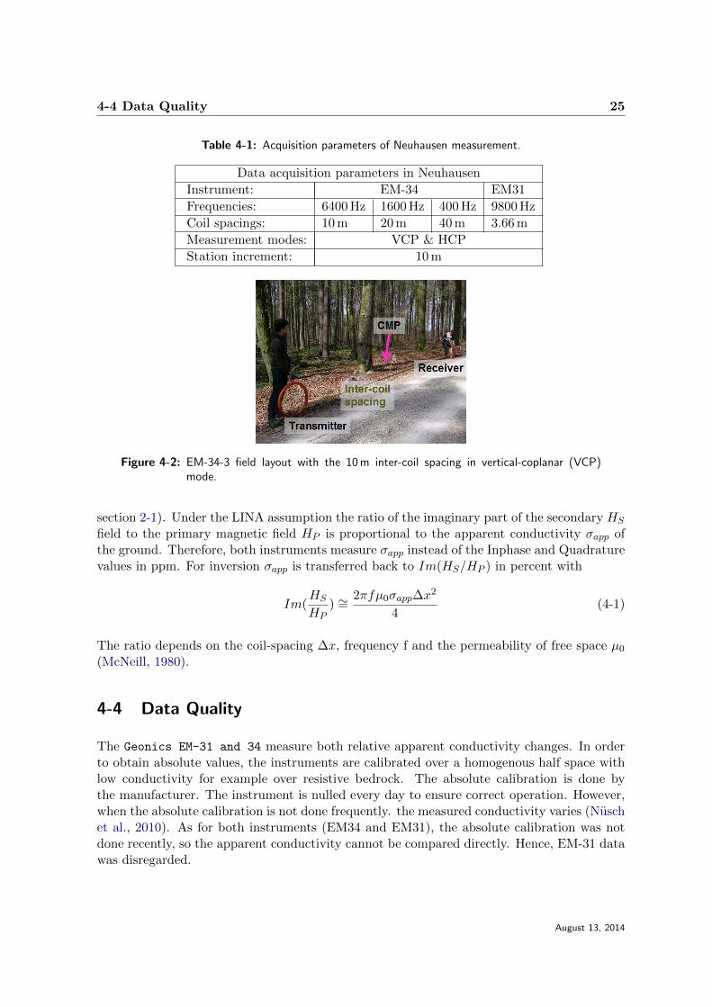
Table 4-1: Acquisition parameters of Neuhausen measurement.
Data acquisition parameters in Neuhausen
Instrument: EM-34 EM31
Frequencies: 6400 Hz 1600 Hz 400 Hz 9800 Hz
Coil spacings: 10 m 20 m 40 m 3.66 m
Measurement modes: VCP & HCP
Station increment: 10 m
Figure 4-2: EM-34-3 field layout with the 10 m inter-coil spacing in vertical-coplanar (VCP)mode.
section 2-1). Under the LINA assumption the ratio of the imaginary part of the secondary HS
field to the primary magnetic field HP is proportional to the apparent conductivity σapp ofthe ground. Therefore, both instruments measure σapp instead of the Inphase and Quadraturevalues in ppm. For inversion σapp is transferred back to Im(HS/HP ) in percent with
Im(HS
HP) ∼=
2πfµ0σapp∆x2
4(4-1)
The ratio depends on the coil-spacing ∆x, frequency f and the permeability of free space µ0
(McNeill, 1980).
4-4 Data Quality
The Geonics EM-31 and 34 measure both relative apparent conductivity changes. In orderto obtain absolute values, the instruments are calibrated over a homogenous half space withlow conductivity for example over resistive bedrock. The absolute calibration is done bythe manufacturer. The instrument is nulled every day to ensure correct operation. However,when the absolute calibration is not done frequently. the measured conductivity varies (Nuschet al., 2010). As for both instruments (EM34 and EM31), the absolute calibration was notdone recently, so the apparent conductivity cannot be compared directly. Hence, EM-31 datawas disregarded.
August 13, 2014
26 Neuhausen: Site and Data Acquisition
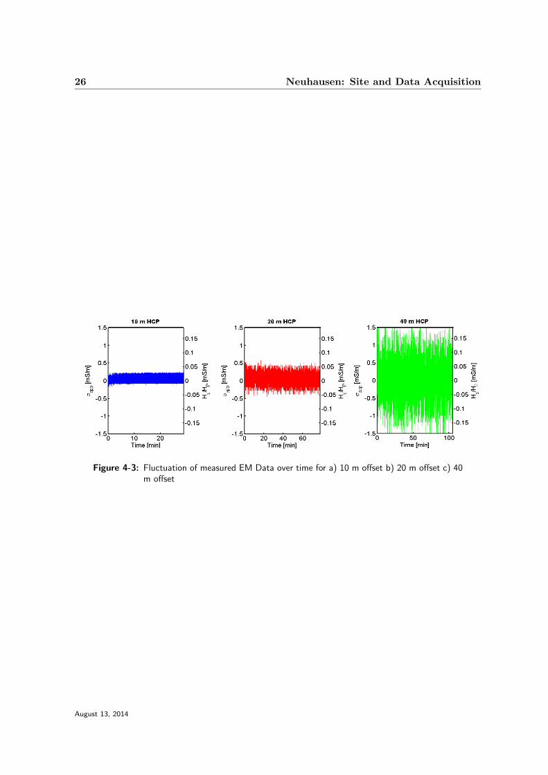
Figure 4-3: Fluctuation of measured EM Data over time for a) 10 m offset b) 20 m offset c) 40m offset
August 13, 2014
Chapter 5
Neuhausen: Inversion Results andDiscussion
In the framework of this chapter, the inversion of the acquired field is shown and discussed.Firstly, the data were inverted 1D with the damped Occam method and afterwards the dataof all lines were inverted with the newly developed pseudo 2D inversion code. Then, thetwo inversion methods are compared and the benefit of the pseudo 2D inversion is discussed.Finally, the depth of investigation is determined. In this chapter, the inversion is shown onthe basis of line 2. The results of Line 1 and 3 can be found in Appendix B.
5-1 Inversion
The infill of the Quaternary valley is complex, no sharp resistivity contrast are expected withinthe sediments. Therefore, I inverted the field data with the damped Occam inversion schemein 1D and in pseudo 2D with lateral and vertical smoothing constraints. Both inversionschemes solved for a multi-layer model with 20 layers. The confining half space starts at adepth of 46 m. The start model used is homogenous with 300 Ωm.
Inversions with all field data resulted in RMS misfits higher than 5. In Figure 5-1 the fielddata of EM-34-3 is compared to the synthetic data from a resulting model. It is clearlyrecognizable that the misfits for 20 m VCP and both 40 m offsets are significant, especially inareas with high apparent conductivity contrast between the measurements. Similar problemswith the 20 m VCP and 40 m were seen also by Monteiro Santos (2004); Kamm et al. (2013).They assumed calibration problems between the offsets geometries. As a consequence, fora good data fit both 10 m modes and the 20 m HCP modes are used in the inversion whichunfortunately results in a loss of depth penetration.
August 13, 2014
28 Inversion Results and Discussion
Figure 5-1: A comparison of the EM34-3 field data (solid line) and forward data (dashed line)from inversion of Line 3. A discrepancy between the synthetic data of both 40 moffset modes and the 20 m VCP mode and their field data is noticeable.
5-1-1 1D Inversion
In 1D inversion, the data of each station is inverted individually, allowing therefore differentdamping factors. A fixed Lagrange multiplier λ2 = 0.5 for smoothing constraints resulted inthe best models. The inversion converged at 20 stations to RMS 1 within 20 iterations. Forthe other 26 stations an RMS misfit between 1 and 2 is observed after 20 iterations. Theaverage RMS misfit is 1.2. The resulting 1D models smoothed only in vertical direction arestitched together and plotted as a pseudo 2D section in Figure 5-2. At the left and right endof the profile, horizontal resistivity changes of 200 Ωm are recognizable. Consequently it ishard to recognize any continuous layer. Only in the middle from x=550-700m a horizontallystretched resistive (500 Ωm) zone can be identified with one significantly different model at640m (green arrow).
August 13, 2014

5-1 Inversion 29
Figure 5-2: Line 2: Stitched 1D vertical smoothness constraint inversion with RMS misfits inthe bottom panel. The green arrow indicates the outlier in the resistive zone
Figure 5-3: Line 2: Pseudo 2D inversion with equal horizontal and vertical smoothness con-straint. RMS misfit in the bottom panel. The blue arrows indicates the lateralresistivity change disappearing with higher horizontal smoothing. The pink ellipsoidmark the conductive zone and
August 13, 2014
30 Inversion Results and Discussion
5-1-2 Pseudo 2D inversion
Through a constant station spacing of 10 m, computing the pseudo 2D smoothness matrixfrom spatial gradients (with respect to height and width of model cell) mainly affects thevertical smoothing as layer thickness increases with depth. So only the absolute differencebetween resistivity is smoothed. By simultaneously inverting the data of all stations together,the line search for the damping factor λ1 results in the same damping factor for all stations,whereas in the 1D inversion for each station a different damping factor resulted.
Figure 5-3 shows the inversion results with a horizontal and vertical smoothness weight of 1.The inversion of all soundings stopped after the maximum of 20 iterations with an averageRMS of 2.
There is a high resistive layer visible, starting in the west at a depth of 20 m and thengradually rising to the surface. After x=700m the resistive layer sinks to 20 m again and endsat 870 m along the line. To the west the resistive layer is covered by a constant conductivezone with 50 Ωm (marked with pink ellipsoid). To the east the cover is more resistive andmore heterogeneous and is marked in Figure 5-3 with a black ellipsoid.
Due to the low lateral constraint of weight 1 the model allows sharp lateral changes, asobserved by the resistive change at x=870 m (marked with a blue arrow). With a higherlateral constraint weight of 7 (Figure 5-4), the deeper less resistive zone to the east disappears.Furthermore, to the west the resistive layer uplift is flattened. The higher RMS clearly showsthe over smoothing in these areas.
Figure 5-4: Line 2: Pseudo 2D horizontal smoothing was 7 times stronger than the verticalsmoothing. The blue arrow indicates the over-smoothed resitivity compared to Fig-ure 5-3. RMS misfits in the bottom panel.
August 13, 2014
5-2 Comparison of 1D and pseudo 2D inversions 31
5-2 Comparison of 1D and pseudo 2D inversions
The stitched together 1D inversion models reveal the same overall characteristics as the pseudo2D models. In the 1D inversion for each station an individual damping factor search is applied,resulting in higher flexibility of the 1D inversion results. Through the lateral resistivitychanges and bumpy features it is, however, hard to interpret.
The pseudo 2D inversion results in smoother more homogenous models. The RMS misfitis however higher than for the 1D models. Siemon et al. (2009) tested a similar pseudo 2Dinversion scheme with synthetic 3D data, in this pseudo 2D inversion the data misfit increasedand the model misfit decreased compared to 1D inversions. Similar it can be assumed that thepseudo 2D inversion model explain the Quaternary valley better than the 1D models. Thelateral smoothing ensures a simple to interpret model which is probably no more complexthan the subsurface. However, non-layered earth structures are perhaps smoothed too much.
5-3 Depth of Investigation
Inversion gives a non-unique model. Consequently, the question is which features of therecovered model resemble the true earth and to what level the depth information of themodel is reliable. The depth of the investigation index (DOI) was determined according toOldenburg and Li (1999) by using different constant start models m1r,m2r. The recoveredmodels are m1r and m2r, so we can define:
DOI(x, z) =m1(x, z)−m2(x, z)
m1r −m2r(5-1)
In areas where the inversions with different start models produce the same results, the DOIapproaches zero. The DOI approaches one at locations where the recovered model is equal tothe start model. Consequently, high DOI indicates areas in which the model is not constrainedby the data. As a consequence, in region with a DOI higher than 0.2, low credibility isassigned. In Figure 5-5 a) and b) the results of pseudo 2D inversions with homogenousstart models of 50 Ω(a) and 1000 Ω (b)with the previously discussed inversion parameters areshown. Both models have an average RMS misfit of 2.1. The general structure is the same inboth recovered models. However, the resistivity in the lower middle part of a) marked witha pink ellipsoid in Figure 5-5 a)) in is lower than in model b). But as the DOI is still lowerthan 0.2, the model is still good resolved. Just on top of this zone at x=750 m(arrow), theDOI is high indicating a zone not constrained by data. The high resistive part in the westand east is slightly higher in b) than in a). This explains the high DOI (seen in Figure 5-5b) in this resistive zone. But as the resistivity for both is high and FDEM methods aregenerally not sensitive to resistive zones, a resistive area is expected but without trust in theabsolute values. As on the other Lines the DOI deeper than 30 m was also high, the modelare trustworthy until a depth of 30 m.
August 13, 2014
32 Inversion Results and Discussion
Figure 5-5: Resistivity models of line 2 generated with a constant start model of a) 50 Ω b) 1000Ω. Both models were inverted with the same parameters and show a similar RMSof around 2.1. The pink ellipsoid indicates the zone with the most visible resistivitychanges. In c) the depth of the investigation index (DOI) of the given models isshown.
5-4 Comparison FDEM and ERT
The 2D ERT measurements were conducted along all three lines using a SyscalPro instrumentwith 96 electrodes at 5 m spacing. The quadrupole measurements are a combination of dipole-dipole, Werner and gradient-array configurations. For covering lines with a length of 970 mthe setup was moved in 250 m steps along the line. After removing poorly galvanically coupledelectrodes and quadripoles with large reciprocity errors, the combined data at each line wereinverted using the boundless electric resistivity tomography tool BERT(Gunther et al., 2006)For the shallow part (less than 100 m) the inverted resistivity distribution explains the datawith a maximum RMS-error of 4.5%. Here I show only the section coinciding with thecoverage of the FDEM data. Figure 5-6 (a) shows the ERT inverse model and Figure 5-6 (b)shows the same ERT model but with an overlay of the FDEM pseudo 2D model. Note thatthe FDEM measurements were done on average 50 m north of the ERT line, along an easieraccessible street. Therefore, the more conductive top meter in FDEM model from x=600m to800m is probably due to the road material. On Line 1 (Figure 5-7) and Line 3 (Figure 5-8),FDEM and ERT measurements were conducted at the same positions.
The absolute values of conductivity of ERT and FDEM are not directly comparable. WhereasERT current electrodes are truly galvanically coupled and FDEM sources are inductivelycoupled. Hence, in ERT the current flow horizontal and vertical, whereas in FDEM with onlyhorizontal current flow in layered media (Lavoue et al., 2010).
August 13, 2014
5-4 Comparison FDEM and ERT 33
Figure 5-6: Line 2: a) ERT model section coinciding with the coverage of the FDEM data. b)FDEM Pseudo 2D model plotted station wise at CMP on top of the ERT modelsection. The red circle mark the zones where conductivities differ the most.
In general, the resistivity models derived from the ERT and FDEM data show a similardistribution and similar values. The deeper conductive structures in the ERT section are notdetected by the FDEM method. Either they are inversion artifacts or are not detected by theFDEM through the low sensitivities in deeper areas by not using the 40 m coil spacing. Asthe DOI values figure(5-3) in this region are higher than 0.1 the latter is probably the case.
In the deeper region of the Quaternary valley infill (e.g. Line 1 from 250m 500m and onLine 2 the west 50 m, marked with a red circle), the ERT and FDEM models disagree themost. One reason could be 3D effects, caused by the complex distribution of the quaternarysediments. 3D effects cannot be accounted for with 1D inversions and introduce artifactualstructure to inverse models (Pellerin and Wannamaker, 2005). Furthermore, the ERT modelhas a higher resolution and is therefore more capable of resolving small heterogeneity in thesediments than FDEM. Overall the FDEM and ERT are in good agreement.
The agreement of our pseudo 2D models and 1D models with the ERT models provides proofthat inversion with 1D forward calculation can describe 2D geological environments.
August 13, 2014
34 Inversion Results and Discussion
Figure 5-7: Line 1: FDEM Pseudo 2D model plotted station wise at CMP on top of the coincidingERT model section. Divided in 2 section: a) first 400 m and b) last 500 m. The redcircle mark the zones where conductivities differ the most.
Figure 5-8: Line 3: FDEM Pseudo 2D model plotted station wise at CMP on top of the coincidingERT model section.
August 13, 2014
Chapter 6
Neuhausen: Geological Interpretation
To interpret the models it is important to notice that Line 2 is plotted within a resistivityrange of 0-500 Ω m whereas for Lines 1 and 3 the range is limited to 300 Ωm.
In Line 2 high resistivity around 500 Ωm at the surface from x=600-750 m match the limestoneindicated on the geological map (Figure 4-1). The change from limestone to quaternarysediments at the edge of the valley is the change from resistive to conductive material. Theresistive limestone dips below the conductive sediments. The medium resistivity (120-300 Ωm)zone at the surface last of x=750m correlates with the dry moraine sediments of the geologicalmap.
The low resistivity 50-100Ωm area at the eastern end of line 3 also has a clear VP /VS ratioanomaly (Schmelzbach et al., 2014). The P-wave velocity increases, while the S-wave velocityis constant. This indicates a higher water content which also explains the low resistivity inthe ERT and FDEM models.
As mentioned in Chapter 2-2-1 the conductivity of of the Quaternary sediments mostly dependon the water content. So here I only divide them in dry and water saturated sediments.However as the resistivity range for dry Quaternary sediments reaches up to 1000Ωm andoverlap with the resistivity range of the limestone. Therefore with resistivity alone bedrockand dry Quaternary sediments can not not clearly differentiated.
A possible interpretation scheme is:
• Bedrock is assumed to have a resistivity of around 400-500 Ωm.
• Low resistivity between 50-100 Ωm is assumed to indicate water saturated Quaternarysediments.
• Medium resistivity between 120-300 Ωm is assumed to indicate dry Quaternary sedi-ments.
August 13, 2014

36 Neuhausen: Interpretation
August 13, 2014

Part II
Glaciological Problem, Site 2, Sea-IcePressure Ridge, ”Barrow”, Alaska
August 13, 2014


Chapter 7
Alaska: Site and Data Acquisition
7-1 Motivation
Deformed sea-ice requests a simple two layer case with a sharp layer interface between ice andsalt water. Due to the simplicity of the problem, FDEM measurements on level sea-ice candirectly be converted into sea-ice thickness. The simple 2-layer assumption fails on sea-icepressure ridges where the ice was crushed and stacked into a 3D structure. The question is ifpseudo 2D inversion of multi frequency EM data helps to get a more realistic image of sea-icepressure ridges.
7-2 Investigation Site
The ETH together with the Alfred Wegener Institute for Polar and Marine Research(AWI)and the University of Alaska fairbanks carried out an extensive study of a first-year pressuresea-ice ridge in the landfast sea ice west of Barrow, Alaska, in April 2011. The selected ridgeshown in Figure 7-1 was chosen to resemble a 2D ridge geometry. This reduces the complexityof the pressure ridge problem as much as possible.
The ridge was surveyed with the following methods: Surface Nuclear Magnetic Resonance(SNMR), Electromagnetic induction (EM), Electrical Resistivity Tomography (ERT), steamdrilling and differential GPS. For further details of the ERT and SNMR results, please referto Hendricks et al. (2011) and Nuber et al. (2013).The measurements were conducted alongthree lines with a length of 100 m and a line spacing of 10 m. EM data was collected on all3 lines. In this thesis, the middle line with x=0m is referred to as Line 1, Line 2 is at x=10 m and Line 3 at x= -10 m. Drilled sea-ice thickness information is only available on line 3with a point spacing of 5 m. The surface topography of the ice ridge is much better sampledwith GPS measurements on all three lines at a spacing of 1 m. The so obtained geometry ofthe sea-ice ridge is shown in Figure 7-2 with zero meters set to the local sea level. The first35 m is undisturbed ice with a depth of 1.3 m. The ridge starts at y=-15 m and its highest
August 13, 2014
40 Alaska: Site and Data Acquisition
Figure 7-1: Layout of measurements of a multi-sensor study of a sea-ice pressure ridge in landfastsea ice. Three lines with an individual length of 100 m and a spacing of 10 meterswere used to align data collected from EM sensors and drilling (Hendricks et al.,2011)
.
−50 −40 −30 −20 −10 0 10 20 30 40 50
−4
−2
0
2
4
6
8
10
12
Distance [m]
De
pth
[m
]
Structure of Ridge
Cavities
Sail
Water
Level Ice
Shallow Keel
Deeper KeelSeparated Porous Keel
Figure 7-2: Line 3 x= -10 m: Topography of ridge and sea-ice thickness obtained from steamdrilling with locations of the voids (blue) found in the boreholes in the ridge .
August 13, 2014
7-3 Data Acquisition 41
point is at y=0 m . Based on the distribution of cavities with a vertical length larger than0.2 m, the ridge is subdivided into three sections. The first two sections are the shallow solidand the deeper porous part of the main keel from y=15 m to 35 m. The shallow keel has lowwater content, whereas the deep keel has relatively high water content. The maximum depthof 11.8 m is at y=5 m. The third section is a separate very porous keel starting at y=35 mand has a high water content.
7-3 Data Acquisition
The multi-frequency EM data were measured with a GEM-2 instrument. The used measure-ments parameters for the GEM instrument are shown in Table 7-1. The GEM instrumenthas a fixed coil-spacing of 1.66 m. The four used frequencies are 330 Hz, 990 Hz, 3990 Hz and9990 Hz. The three lines were surveyed with 1 m steps using three measurements modes: twohorizontal coplanar (HCP) configurations (sensor aligned along-track and across-track) onthe ground and a vertical-coplanar(VCP) configuration at hip height. The data are shown inthe Appendix C.
Data aquisation parameters
Instrument: GEM-2Frequencies: 330 Hz, 990 Hz, 3990 Hz, 9990 HzCoil spacing: 1.66 mStacking: 1 HzMeasurements mode: VCP (hip height), HCP(on ground)
Table 7-1: Acquisition parameters of GEM measurements.
7-4 Data Quality
The VCP data has unexplained jumps in the in-phase and negative responses for the lowerfrequencies (see Figure 7-3). As no explanation could be found, the VCP data set was notused. For the HCP data set, an absolute uncertainty of 200 ppm is assumed as discussed inHendricks et al. (2011).
August 13, 2014
42 Alaska: Site and Data Acquisition
Figure 7-3: a) Horizontal coplanar (HCP) GEM-2 and b) Vertical coplanar (VCP) data of ridgeat line 3 x=-10m.
August 13, 2014
Chapter 8
Alaska: Inversion Results andDiscussion
Within the scope of this chapter, I will explain the problems caused by the GEM bucking coilin the vicinity of highly conductive ocean water and discuss a possible solution for the forwardcalculation of GEM data on sea-ice. The bucking correction was then used in the 1D andpseudo 2D inversion. Finally, the potential of multi-frequency EM data on ice is discussed.
8-1 Bucking Coil Correction
The GEM-2 instrument consists of 3 coils: the transmitter (Tx) coil, the receiver (Rx) coiland the bucking (Bx) coil (Figure 8-1). The transmitter-receiver coil spacing is 1.66 m. Thetransmitter-bucking coil spacing is 1.035 m. The wiring of the bucking coil is set in orderto eliminate the primary magnetic field at the receiver coil. The bucking coil measures anequally strong opposite primary magnetic field and only a small constant secondary magneticfield which can be neglected. By overlapping the receiver signal with the bucking signal onlythe secondary magnetic field results at the receiver.
Figure 8-1: Scheme of the GEM-2 instrument. The receiver and transmitter coils are at the endof the instruments with a spacing of 166 cm. The bucking coil is at a distance of1.035 m from the transmitter.
August 13, 2014
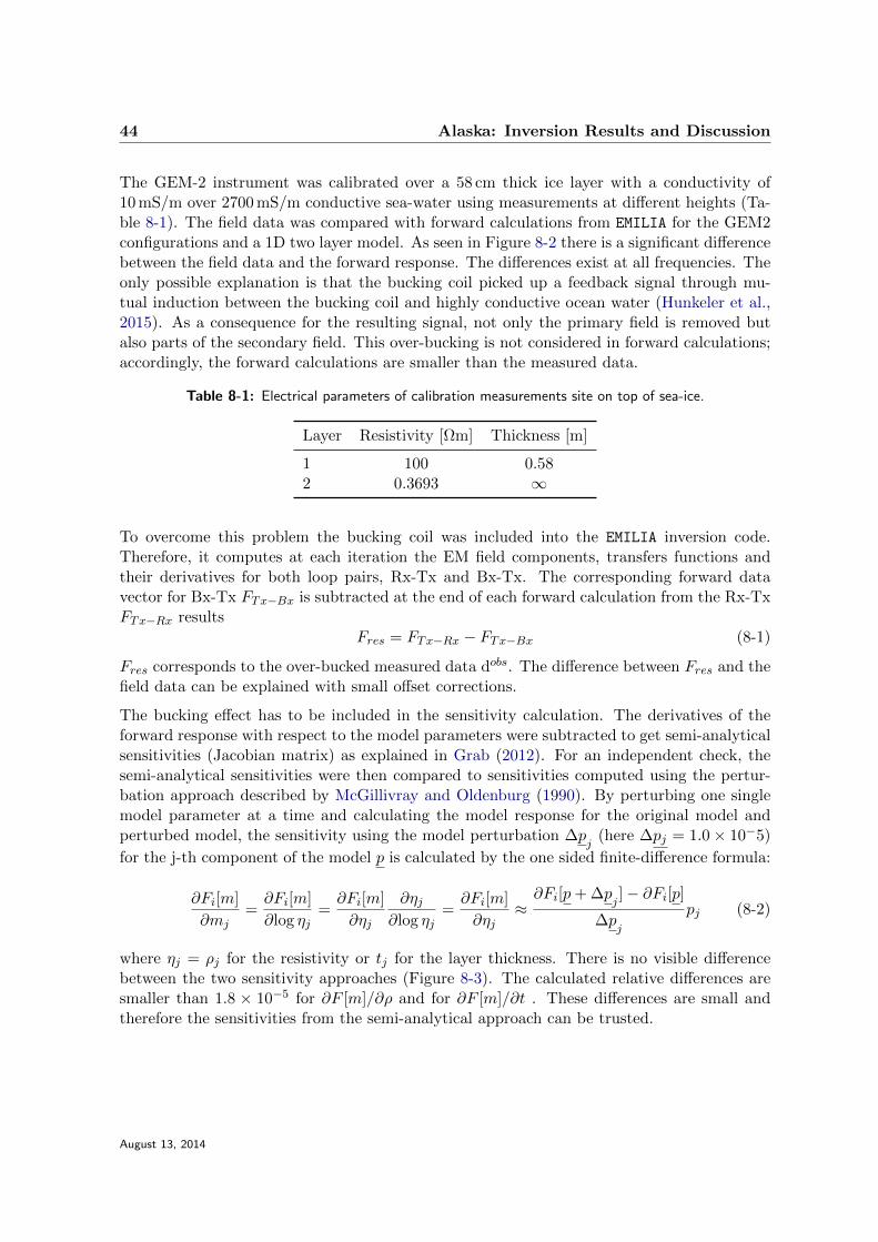
44 Alaska: Inversion Results and Discussion
The GEM-2 instrument was calibrated over a 58 cm thick ice layer with a conductivity of10 mS/m over 2700 mS/m conductive sea-water using measurements at different heights (Ta-ble 8-1). The field data was compared with forward calculations from EMILIA for the GEM2configurations and a 1D two layer model. As seen in Figure 8-2 there is a significant differencebetween the field data and the forward response. The differences exist at all frequencies. Theonly possible explanation is that the bucking coil picked up a feedback signal through mu-tual induction between the bucking coil and highly conductive ocean water (Hunkeler et al.,2015). As a consequence for the resulting signal, not only the primary field is removed butalso parts of the secondary field. This over-bucking is not considered in forward calculations;accordingly, the forward calculations are smaller than the measured data.
Table 8-1: Electrical parameters of calibration measurements site on top of sea-ice.
Layer Resistivity [Ωm] Thickness [m]
1 100 0.582 0.3693 ∞
To overcome this problem the bucking coil was included into the EMILIA inversion code.Therefore, it computes at each iteration the EM field components, transfers functions andtheir derivatives for both loop pairs, Rx-Tx and Bx-Tx. The corresponding forward datavector for Bx-Tx FTx−Bx is subtracted at the end of each forward calculation from the Rx-TxFTx−Rx results
Fres = FTx−Rx − FTx−Bx (8-1)
Fres corresponds to the over-bucked measured data dobs. The difference between Fres and thefield data can be explained with small offset corrections.
The bucking effect has to be included in the sensitivity calculation. The derivatives of theforward response with respect to the model parameters were subtracted to get semi-analyticalsensitivities (Jacobian matrix) as explained in Grab (2012). For an independent check, thesemi-analytical sensitivities were then compared to sensitivities computed using the pertur-bation approach described by McGillivray and Oldenburg (1990). By perturbing one singlemodel parameter at a time and calculating the model response for the original model andperturbed model, the sensitivity using the model perturbation ∆p
j(here ∆pj = 1.0× 10⁻⁵)
for the j-th component of the model p is calculated by the one sided finite-difference formula:
∂Fi[m]
∂mj=∂Fi[m]
∂log ηj=∂Fi[m]
∂ηj
∂ηj∂log ηj
=∂Fi[m]
∂ηj≈∂Fi[p+ ∆p
j]− ∂Fi[p]
∆pj
pj (8-2)
where ηj = ρj for the resistivity or tj for the layer thickness. There is no visible differencebetween the two sensitivity approaches (Figure 8-3). The calculated relative differences aresmaller than 1.8 × 10⁻⁵ for ∂F [m]/∂ρ and for ∂F [m]/∂t . These differences are small andtherefore the sensitivities from the semi-analytical approach can be trusted.
August 13, 2014
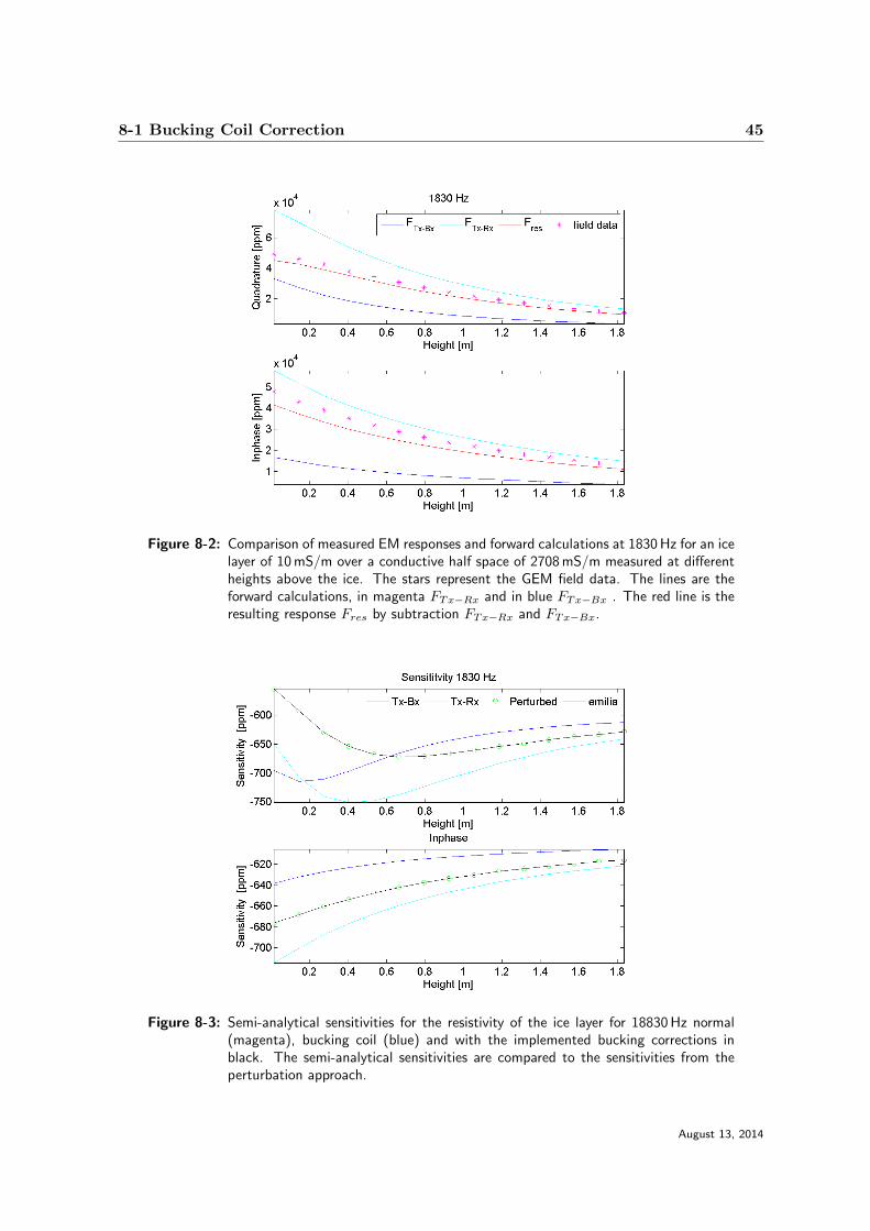
8-1 Bucking Coil Correction 45
Figure 8-2: Comparison of measured EM responses and forward calculations at 1830 Hz for an icelayer of 10 mS/m over a conductive half space of 2708 mS/m measured at differentheights above the ice. The stars represent the GEM field data. The lines are theforward calculations, in magenta FTx−Rx and in blue FTx−Bx . The red line is theresulting response Fres by subtraction FTx−Rx and FTx−Bx.
Figure 8-3: Semi-analytical sensitivities for the resistivity of the ice layer for 18830 Hz normal(magenta), bucking coil (blue) and with the implemented bucking corrections inblack. The semi-analytical sensitivities are compared to the sensitivities from theperturbation approach.
August 13, 2014
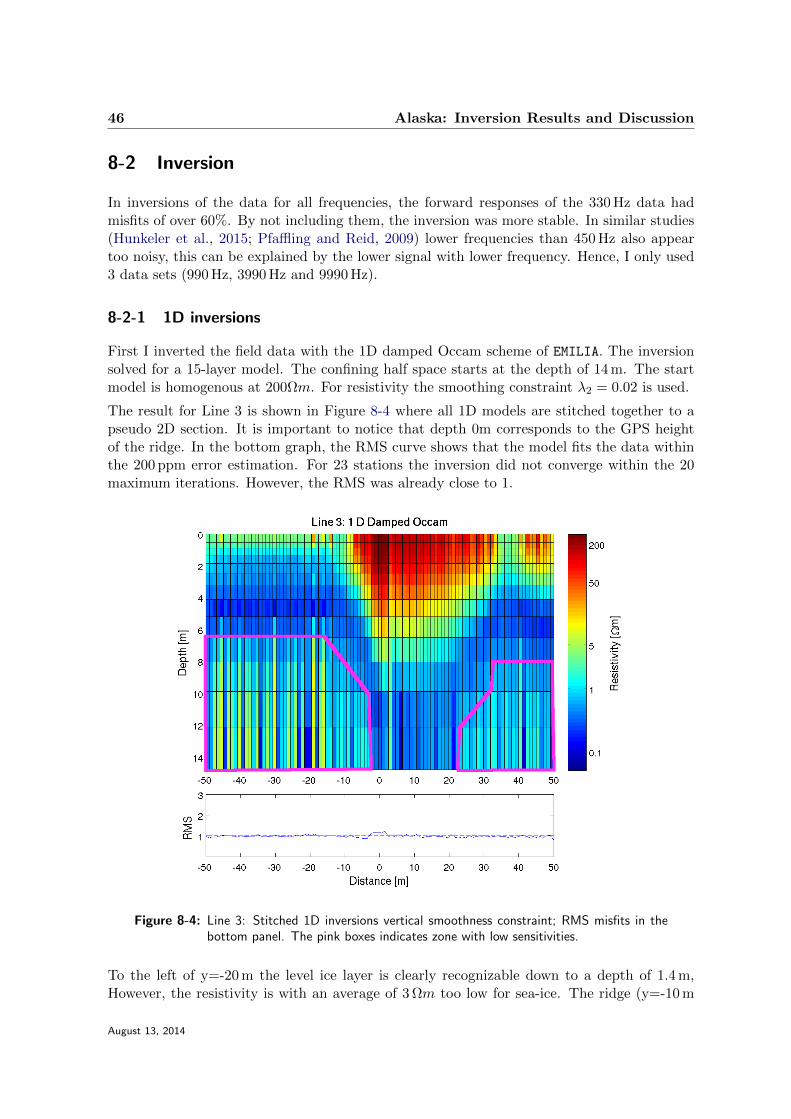
46 Alaska: Inversion Results and Discussion
8-2 Inversion
In inversions of the data for all frequencies, the forward responses of the 330 Hz data hadmisfits of over 60%. By not including them, the inversion was more stable. In similar studies(Hunkeler et al., 2015; Pfaffling and Reid, 2009) lower frequencies than 450 Hz also appeartoo noisy, this can be explained by the lower signal with lower frequency. Hence, I only used3 data sets (990 Hz, 3990 Hz and 9990 Hz).
8-2-1 1D inversions
First I inverted the field data with the 1D damped Occam scheme of EMILIA. The inversionsolved for a 15-layer model. The confining half space starts at the depth of 14 m. The startmodel is homogenous at 200Ωm. For resistivity the smoothing constraint λ2 = 0.02 is used.
The result for Line 3 is shown in Figure 8-4 where all 1D models are stitched together to apseudo 2D section. It is important to notice that depth 0m corresponds to the GPS heightof the ridge. In the bottom graph, the RMS curve shows that the model fits the data withinthe 200 ppm error estimation. For 23 stations the inversion did not converge within the 20maximum iterations. However, the RMS was already close to 1.
Figure 8-4: Line 3: Stitched 1D inversions vertical smoothness constraint; RMS misfits in thebottom panel. The pink boxes indicates zone with low sensitivities.
To the left of y=-20 m the level ice layer is clearly recognizable down to a depth of 1.4 m,However, the resistivity is with an average of 3 Ωm too low for sea-ice. The ridge (y=-10 m
August 13, 2014
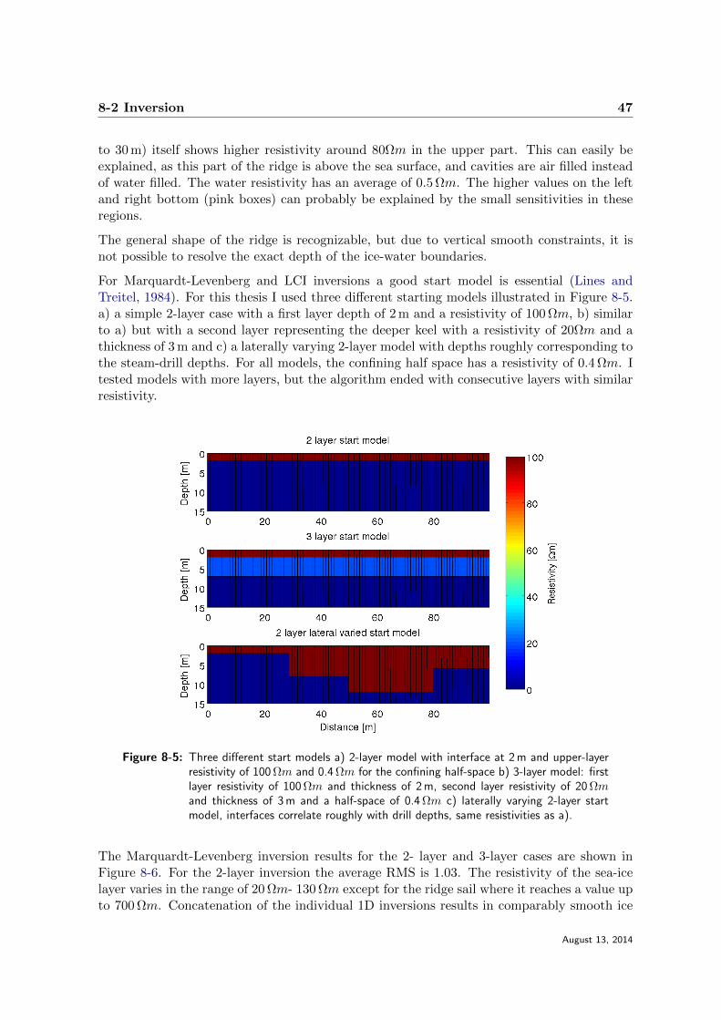
8-2 Inversion 47
to 30 m) itself shows higher resistivity around 80Ωm in the upper part. This can easily beexplained, as this part of the ridge is above the sea surface, and cavities are air filled insteadof water filled. The water resistivity has an average of 0.5 Ωm. The higher values on the leftand right bottom (pink boxes) can probably be explained by the small sensitivities in theseregions.
The general shape of the ridge is recognizable, but due to vertical smooth constraints, it isnot possible to resolve the exact depth of the ice-water boundaries.
For Marquardt-Levenberg and LCI inversions a good start model is essential (Lines andTreitel, 1984). For this thesis I used three different starting models illustrated in Figure 8-5.a) a simple 2-layer case with a first layer depth of 2 m and a resistivity of 100 Ωm, b) similarto a) but with a second layer representing the deeper keel with a resistivity of 20Ωm and athickness of 3 m and c) a laterally varying 2-layer model with depths roughly corresponding tothe steam-drill depths. For all models, the confining half space has a resistivity of 0.4 Ωm. Itested models with more layers, but the algorithm ended with consecutive layers with similarresistivity.
Figure 8-5: Three different start models a) 2-layer model with interface at 2 m and upper-layerresistivity of 100 Ωm and 0.4 Ωm for the confining half-space b) 3-layer model: firstlayer resistivity of 100 Ωm and thickness of 2 m, second layer resistivity of 20 Ωmand thickness of 3 m and a half-space of 0.4 Ωm c) laterally varying 2-layer startmodel, interfaces correlate roughly with drill depths, same resistivities as a).
The Marquardt-Levenberg inversion results for the 2- layer and 3-layer cases are shown inFigure 8-6. For the 2-layer inversion the average RMS is 1.03. The resistivity of the sea-icelayer varies in the range of 20 Ωm- 130 Ωm except for the ridge sail where it reaches a value upto 700 Ωm. Concatenation of the individual 1D inversions results in comparably smooth ice
August 13, 2014
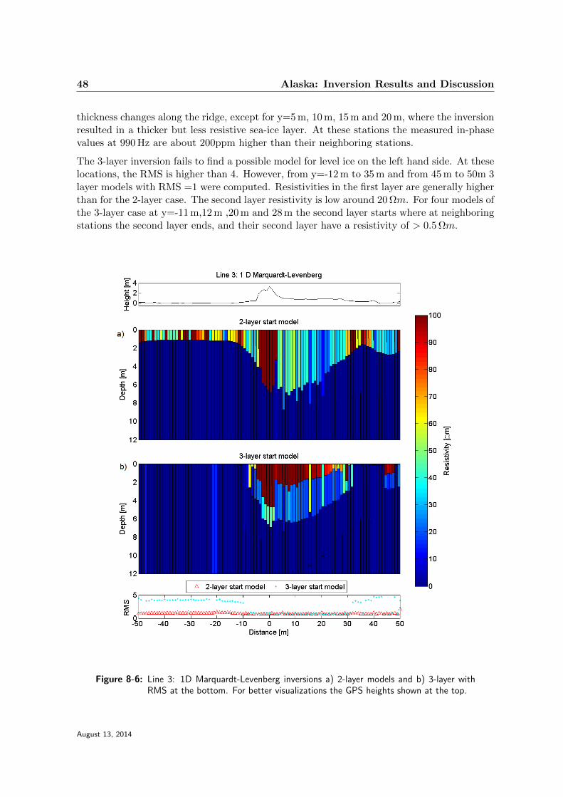
48 Alaska: Inversion Results and Discussion
thickness changes along the ridge, except for y=5 m, 10 m, 15 m and 20 m, where the inversionresulted in a thicker but less resistive sea-ice layer. At these stations the measured in-phasevalues at 990 Hz are about 200ppm higher than their neighboring stations.
The 3-layer inversion fails to find a possible model for level ice on the left hand side. At theselocations, the RMS is higher than 4. However, from y=-12 m to 35 m and from 45 m to 50m 3layer models with RMS =1 were computed. Resistivities in the first layer are generally higherthan for the 2-layer case. The second layer resistivity is low around 20 Ωm. For four models ofthe 3-layer case at y=-11 m,12 m ,20 m and 28 m the second layer starts where at neighboringstations the second layer ends, and their second layer have a resistivity of > 0.5 Ωm.
Figure 8-6: Line 3: 1D Marquardt-Levenberg inversions a) 2-layer models and b) 3-layer withRMS at the bottom. For better visualizations the GPS heights shown at the top.
August 13, 2014
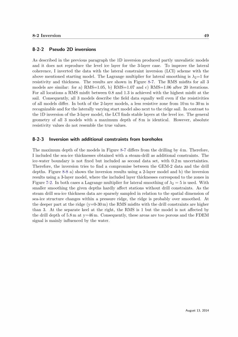
8-2 Inversion 49
8-2-2 Pseudo 2D inversions
As described in the previous paragraph the 1D inversion produced partly unrealistic modelsand it does not reproduce the level ice layer for the 3-layer case. To improve the lateralcoherence, I inverted the data with the lateral constraint inversion (LCI) scheme with theabove mentioned starting model. The Lagrange multiplier for lateral smoothing is λ2=1 forresistivity and thickness. The results are shown in Figure 8-7. The RMS misfits for all 3models are similar: for a) RMS=1.05, b) RMS=1.07 and c) RMS=1.06 after 20 iterations.For all locations a RMS misfit between 0.8 and 1.3 is achieved with the highest misfit at thesail. Consequently, all 3 models describe the field data equally well even if the resistivitiesof all models differ. In both of the 2-layer models, a less resistive zone from 10 m to 30 m isrecognizable and for the laterally varying start model also next to the ridge sail. In contrast tothe 1D inversion of the 3-layer model, the LCI finds stable layers at the level ice. The generalgeometry of all 3 models with a maximum depth of 8 m is identical. However, absoluteresistivity values do not resemble the true values.
8-2-3 Inversion with additional constraints from boreholes
The maximum depth of the models in Figure 8-7 differs from the drilling by 4 m. Therefore,I included the sea-ice thicknesses obtained with a steam-drill as additional constraints. Theice-water boundary is not fixed but included as second data set, with 0.2 m uncertainties.Therefore, the inversion tries to find a compromise between the GEM-2 data and the drilldepths. Figure 8-8 a) shows the inversion results using a 2-layer model and b) the inversionresults using a 3-layer model, where the included layer thicknesses correspond to the zones inFigure 7-2. In both cases a Lagrange multiplier for lateral smoothing of λ2 = 5 is used. Withsmaller smoothing the given depths hardly affect stations without drill constraints. As thesteam drill sea-ice thickness data are sparsely sampled in relation to the spatial dimension ofsea-ice structure changes within a pressure ridge, the ridge is probably over smoothed. Atthe deeper part at the ridge (y=0-30 m) the RMS misfits with the drill constraints are higherthan 3. At the separate keel at the right, the RMS is 1 but the model is not affected bythe drill depth of 5.8 m at y=46 m. Consequently, these areas are too porous and the FDEMsignal is mainly influenced by the water.
August 13, 2014
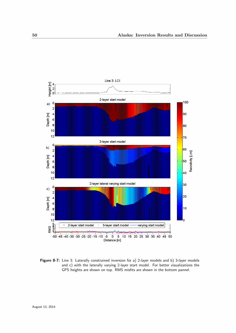
50 Alaska: Inversion Results and Discussion
Figure 8-7: Line 3: Laterally constrained inversion for a) 2-layer models and b) 3-layer modelsand c) with the laterally varying 2-layer start model. For better visualizations theGPS heights are shown on top. RMS misfits are shown in the bottom pannel.
August 13, 2014
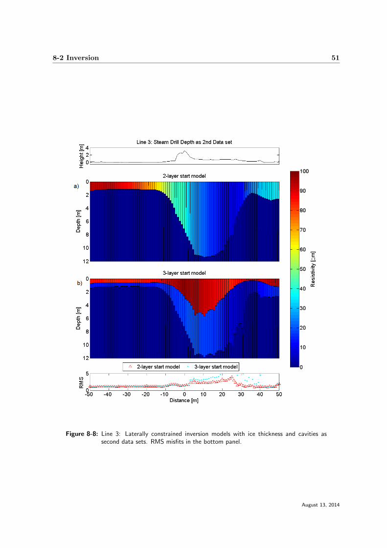
8-2 Inversion 51
Figure 8-8: Line 3: Laterally constrained inversion models with ice thickness and cavities assecond data sets. RMS misfits in the bottom panel.
August 13, 2014

52 Alaska: Inversion Results and Discussion
8-2-4 Single vs. multi-frequency inversions
To estimate the thickness of level sea-ice only one frequency is needed, for example an EM-31instrument with a frequency of 9800 Hz. On deformed sea-ice, where it is hard to define a1D sea-ice thickness, the usage of multi-frequencies provides more observational constraintsin order to obtain a less ambiguous model of the resistivity distribution. However, throughthe small inter-coil spacing of 1.66 m of the GEM-2 instrument the penetration depth ismainly affected by the coil spacing and not frequency. Consequently multi-frequency soundingonly constrain better when data at different frequencies are differently affected by noise. Icompared the results of multi-frequency inversion with single frequency inversion. The resultsfor a single frequency of 9990 Hz are shown in Figure 8-9 and are nearly identical to the modelwith multi-frequencies (Figure 8-7). In the ridge below the sail(pink ellipsoid) the RMS isstill high, indicating probably a lower signal to noise ratio in this area, than in level-ice. Byinverting with a single frequency of 990 Hz or 3990 Hz, the models show the same resistivitypattern but with 3990 Hz the ridge is 0.5 m shallower and with 990 Hz around 0.5 m deeper.All single frequencies inversion converged after 8 iterations, as the overall misfit was below 1.Consequently, multi-frequency data in the range below 10 kHz do not resolve thickness andresistivity distributions in sea-ice ridges better than single frequency surveys.
August 13, 2014
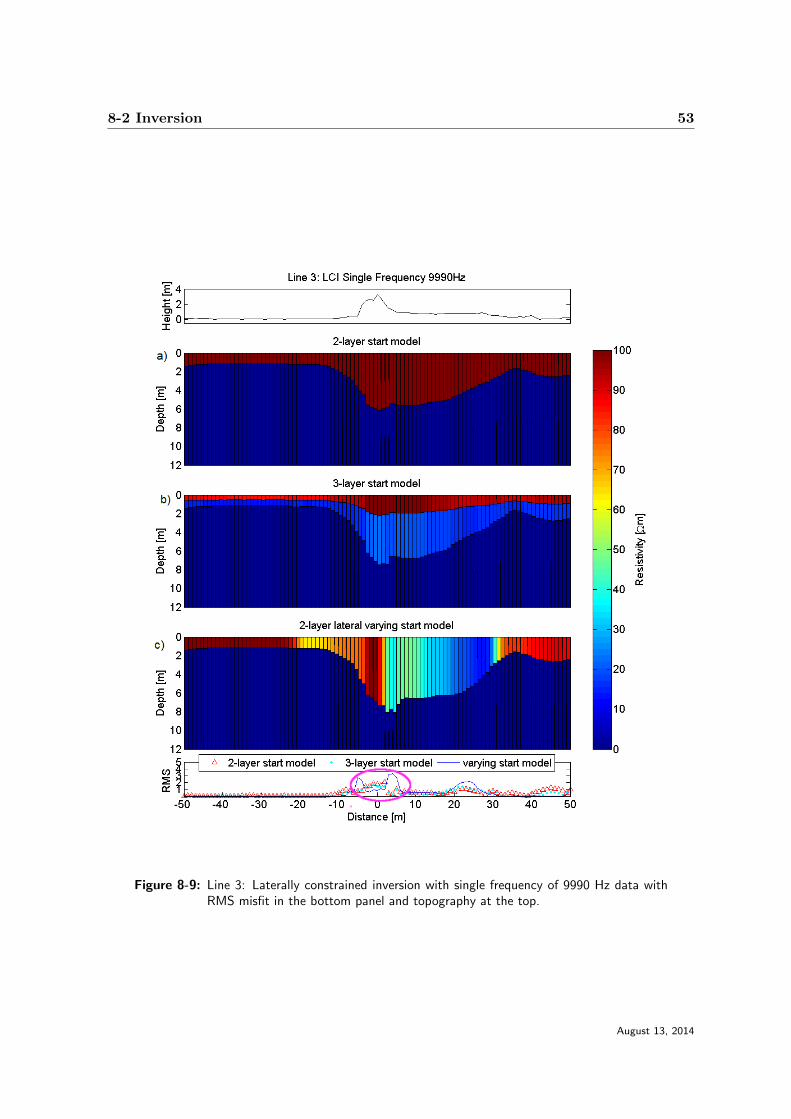
8-2 Inversion 53
Figure 8-9: Line 3: Laterally constrained inversion with single frequency of 9990 Hz data withRMS misfit in the bottom panel and topography at the top.
August 13, 2014
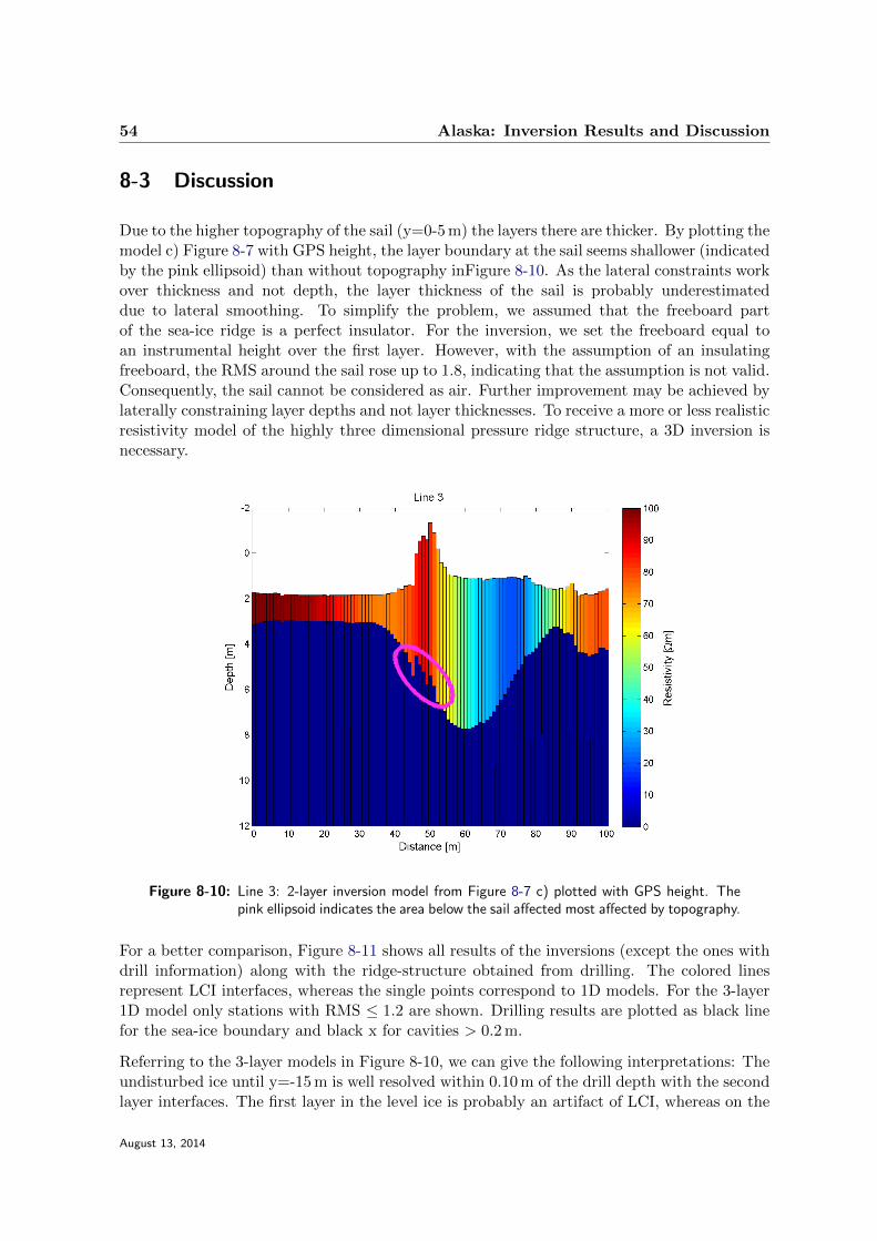
54 Alaska: Inversion Results and Discussion
8-3 Discussion
Due to the higher topography of the sail (y=0-5 m) the layers there are thicker. By plotting themodel c) Figure 8-7 with GPS height, the layer boundary at the sail seems shallower (indicatedby the pink ellipsoid) than without topography inFigure 8-10. As the lateral constraints workover thickness and not depth, the layer thickness of the sail is probably underestimateddue to lateral smoothing. To simplify the problem, we assumed that the freeboard partof the sea-ice ridge is a perfect insulator. For the inversion, we set the freeboard equal toan instrumental height over the first layer. However, with the assumption of an insulatingfreeboard, the RMS around the sail rose up to 1.8, indicating that the assumption is not valid.Consequently, the sail cannot be considered as air. Further improvement may be achieved bylaterally constraining layer depths and not layer thicknesses. To receive a more or less realisticresistivity model of the highly three dimensional pressure ridge structure, a 3D inversion isnecessary.
Figure 8-10: Line 3: 2-layer inversion model from Figure 8-7 c) plotted with GPS height. Thepink ellipsoid indicates the area below the sail affected most affected by topography.
For a better comparison, Figure 8-11 shows all results of the inversions (except the ones withdrill information) along with the ridge-structure obtained from drilling. The colored linesrepresent LCI interfaces, whereas the single points correspond to 1D models. For the 3-layer1D model only stations with RMS ≤ 1.2 are shown. Drilling results are plotted as black linefor the sea-ice boundary and black x for cavities > 0.2 m.
Referring to the 3-layer models in Figure 8-10, we can give the following interpretations: Theundisturbed ice until y=-15 m is well resolved within 0.10 m of the drill depth with the secondlayer interfaces. The first layer in the level ice is probably an artifact of LCI, whereas on the
August 13, 2014
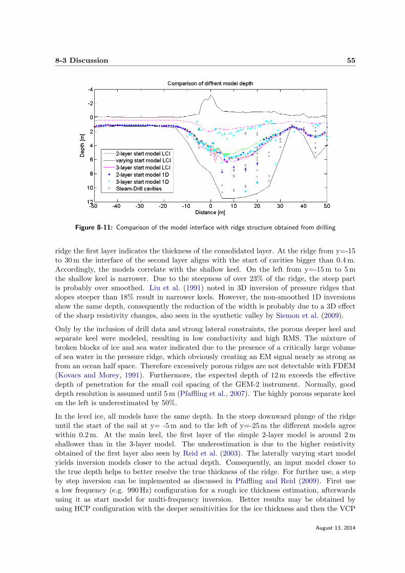
8-3 Discussion 55
Figure 8-11: Comparison of the model interface with ridge structure obtained from drilling
ridge the first layer indicates the thickness of the consolidated layer. At the ridge from y=-15to 30 m the interface of the second layer aligns with the start of cavities bigger than 0.4 m.Accordingly, the models correlate with the shallow keel. On the left from y=-15 m to 5 mthe shallow keel is narrower. Due to the steepness of over 23% of the ridge, the steep partis probably over smoothed. Liu et al. (1991) noted in 3D inversion of pressure ridges thatslopes steeper than 18% result in narrower keels. However, the non-smoothed 1D inversionsshow the same depth, consequently the reduction of the width is probably due to a 3D effectof the sharp resistivity changes, also seen in the synthetic valley by Siemon et al. (2009).
Only by the inclusion of drill data and strong lateral constraints, the porous deeper keel andseparate keel were modeled, resulting in low conductivity and high RMS. The mixture ofbroken blocks of ice and sea water indicated due to the presence of a critically large volumeof sea water in the pressure ridge, which obviously creating an EM signal nearly as strong asfrom an ocean half space. Therefore excessively porous ridges are not detectable with FDEM(Kovacs and Morey, 1991). Furthermore, the expected depth of 12 m exceeds the effectivedepth of penetration for the small coil spacing of the GEM-2 instrument. Normally, gooddepth resolution is assumed until 5 m (Pfaffling et al., 2007). The highly porous separate keelon the left is underestimated by 50%.
In the level ice, all models have the same depth. In the steep downward plunge of the ridgeuntil the start of the sail at y= -5 m and to the left of y=-25 m the different models agreewithin 0.2 m. At the main keel, the first layer of the simple 2-layer model is around 2 mshallower than in the 3-layer model. The underestimation is due to the higher resistivityobtained of the first layer also seen by Reid et al. (2003). The laterally varying start modelyields inversion models closer to the actual depth. Consequently, an input model closer tothe true depth helps to better resolve the true thickness of the ridge. For further use, a stepby step inversion can be implemented as discussed in Pfaffling and Reid (2009). First usea low frequency (e.g. 990 Hz) configuration for a rough ice thickness estimation, afterwardsusing it as start model for multi-frequency inversion. Better results may be obtained byusing HCP configuration with the deeper sensitivities for the ice thickness and then the VCP
August 13, 2014

56 Alaska: Inversion Results and Discussion
configuration for the conductivity.
In all recovered models, the resistivity is not reliable and depends on the start model. Thelevel ice with a depth of 1.4 m is according to Pfaffling and Reid (2009) too thin for stableresults of conductivity for the used frequencies range in our study. Furthermore, for reliableconductivity the GEM-2 instruments need to be better calibrated as noted by Hunkeler et al.(2015). For a reliable sea-ice conductivity estimation, they fixed the thickness for sea-ice andplatelet layer. In our inversion all parameters are allowed to vary. Consequently, the waterconductivity from the inversion differs ±0.1S/m from the exact values of 0.38Sm−1 resultingin uncertainty of the sea-ice conductivity.
The pseudo 2D inversion creates a laterally smooth geometry of a shallow keel of the ridgewithout outliers like in the 1D inversion. However, the deep keel with high porosity is toodeep and too complex to be comprehensively described by 1D inversion of GEM-2 data.
August 13, 2014

Chapter 9
Overall Conclusions and Outlook
9-1 Conclusions
In this thesis, the existing 1D EM inversion component in EMILIA was enhanced for pseudo2D inversion. In pseudo 2D inversion, all data sets are inverted simultaneously for layered1D models minimizing a common objective function with lateral constraints in the modelregularization function.
Two different pseudo 2D inversion schemes were implemented. First, there is a 2D smoothinversion with fixed layer thicknesses. The model regularization contains horizontal andvertical smoothing constraints, resulting in smooth models. Second, a laterally constrainedinversion (LCI) was added in which resistivity and interval thickness of individual layers issmoothed between abutting stations. The output is a laterally smooth 2D model with sharplayer interfaces in the vertical direction.
The pseudo 2D smooth inversion was tested and compared to 1D damped Occam inversionon FDEM field data collected on Quaternary sediments in Neuhausen. The measurementswere performed with Geonics EM-34-3 and EM-31 instruments. The goal was to complementexisting ERT, seismic and TEM data for a near surface model of the Quaternary valley.Both the 1D and pseudo 2D models showed resistivity patterns similar to the ERT models.Therefore, one conclusion is, that inversions with 1D forward calculations and sensitivities areable to describe 2D or 3D geological environments given that multi-dimensional conductivityanomalies are not too pronounced. The pseudo 2D inversion resulted in a smooth model butwith higher RMS misfit than the 1D inversion. However, in 1D resistivity models obtainedwith pure 1D inversion small scale features appear which are very likely not part of the trueearth. For a geological interpretation the pseudo 2D inversion is more suitable.
In the second case study on a sea-ice pressure ridge, the LCI inversion scheme was tested andcompared to 1D Marquardt Levenberg inversions. The data was collected using the multi-frequency GEM-2 instrument. On highly conductive ground such as saline ocean water,the bucking coil measures an inductive feedback, consequently reducing the secondary fieldmeasured at the receiver. This phenomenon was addressed by including the bucking coil
August 13, 2014
58 Overall Conclusions and Outlook
into the forward calculation part EMILIA. Inverted resistivity models visualized a layer ofconsolidated sea-ice, in the level part and in the shallower part of the pressure ridge. Thedeeper and more porous keel with a maximum depth of 12 m could not be imaged by invertingGEM-2 data. Due to the high porosity, the signal is mainly controlled by sea-water pockets,consequently the conductivities do not differ from open water. Furthermore, the coil spacingof 1.66 m of the GEM-2 instrument is too small for good resolution down to 12 m. The LCIinversion resulted in a smoother model with fewer unrealistic 1D model sections than the 1Dinversions. However, in none of the models an estimate of the absolute electrical conductivityis possible.
Tests with different start models showed that a simple 2-layer model underestimated thedepth of the consolidated ridge. With start models with greater depths to the ridge and withstart models with more layers, the ridge is better resolved. However, level ice could not beexplained with 3-layer models. Another important conclusion was that inversion with singlefrequency and multi frequency did not differ significantly.
In summary, one can say that pseudo 2D inversion proved to be of an advantage over pure1D inversion in both cases studies.
9-2 Outlook
The next steps to take with the data from the Quaternary valley in Neuhausen are (1) tojointly invert them with ERT and TEM data, and (2) to add extra constraints from seismicmodels to get an improved image of the sedimentary infill. Ultimately, a near surface modelneeds to be established.
To obtain more reliable resistivity on sea-ice pressure ridges, inversion with fixed water con-ductivity or fixed layer thicknesses should be tested. Then, the inversion would only adjustthe conductivity of the ice and optionally layer thicknesses. The constraint inversion usingknown information (e.g. for water conductivity or level-ice thickness) has less free modelparameters and is better determined. Consequently, the models should be more accurate.Additionally, sensitivities for different frequencies, Tx-Rx heights and Tx-Rx orientations onice need to be compared to find the best measurement setup of the multi-frequency GEM-2instrument on ice. Additionally, different frequency sensitivities on ice need to be comparedto find the best measurement setup of the multi-frequency GEM-2 instrument on ice.
Further improvement of the inversion code may be achieved by applying lateral constraintson elevation instead on layer number to encourage horizontal structures below a bumby to-pography (e.g. sea-ice ridge sail or steep slopes).
August 13, 2014

Acknowledgements
I would like to thank everyone who has contributed in some way to my final thesis. Firstof all I wish to thank my supervisor Dr. Lasse Rabenstein, who introduced me to FDEMand supported me with his knowledge of sea-ice pressure ridges and helped in conducting thefield survey in Neuhausen. Further thanks go to Dr. Thomas Kalscheuer, who introducedme to his emila inversion program and helped me with both my Fortran programming andin organizing my stay in Uppsala. Also I would like to thank Melchior Grab, for helping mewith small EMILIA problems.
I also wish to thank my field crew Willhem Vince Meijer and Andres Clalna who helped meacquiring data at the field site in Neuhausen. Further thanks go to my office colleagues forcheering me up in dark moments and and always sharing thoughts and ideas. Finally, veryspecial thanks go to my parents for supporting me during my Bachelor and Master studies.
Swiss Federal Institute of Technology Manuela Sarah Kaufmann
August 13, 2014
August 13, 2014

60 Acknowledgements
August 13, 2014

Bibliography
Auken, E. and Christiansen, A. V. (2004). Layered and laterally constrained 2D inversion ofresistivity data. Geophysics, 69(3):752–761.
Auken, E., Christiansen, A. V., Jacobsen, B. H., Foged, N., and Srensen, K. I. (2005).Piecewise 1D laterally constrained inversion of resistivity data. Geophysical Prospecting,53(4):497–506.
Christiansen, A. V. and Auken, E. (2004). Optimizing a layered and laterally constrained 2Dinversion of resistivity data using broyden’s update and 1D derivatives. Journal of AppliedGeophysics, 56(4):247 – 261.
Constable, S. C., Parker, R. L., and Constable, C. G. (1987). Occam’s inversion: A practicalalgorithm for generating smooth models from electromagnetic sounding data. Geophysics,52:289–300.
Everett, M. E. and Meju, M. A. (2005). Near-surface controlled-source electromagnetic in-duction. In Hydrogeophysics, pages 157–183. Springer.
Frischknecht, F. C., Labson, V. F., Spies, B. R., and Anderson, W. L. (2001). ElectromagneticMethods in Applied Geophysics, volume 2, chapter Profiling Methods uscing Small Sources,pages 105–270. Soc. Expl. Geophys., Tulsa, Oklahoma.
Grab, M. (2012). Forward and inverse modelling of frequency-domain electromagnetic datafrom small coils. Master’s thesis, ETH Zrich.
Grant, F. S. and West, G. F. (1965). Interpretation Theory in Applied Geophysics. McGraw-Hill Book Company, New York.
Gunther, T., Rucker, C., and Spitzer, K. (2006). Three-dimensional modelling and inver-sion of dc resistivity data incorporating topography ii. inversion. Geophysical JournalInternational, 166(2):506–517.
Hendricks, S., Rabenstein, L., Lehmann-Horn, J., Nuber, A., Eicken, H., and Mahoney, A.(2011). Sizonet 2011, data acquisition report.
August 13, 2014
62 Bibliography
Hunkeler, P. A., Hendricks, S., Mario Hoppmann, S. P., and Gerdes, R. (2015). Towardsan estimation of sub sea-ice platelet-layer volume with multi-frequency electromagneticinduction sounding. Annals of Glaciology, 56. In preparation.
Hyland, K. V. (2002). Consolidation of first-year sea ice ridges. Journal of GeophysicalResearch: Oceans, 107(C6):15–1–15–16.
Kalscheuer, T. (2014). EMILIA - Electro Magnetic Inversion with Least Intricate Algorithms.User manual.
Kalscheuer, T., Hbert, J., Kuvshinov, A., Lochbhler, T., and Pedersen, L. B. (2012). A hybridregularization scheme for the inversion of magnetotelluric data from natural and controlledsources to layer and distortion parameters. Geophysics, 77(4):E301–E315.
Kalscheuer, T., Juanatey, M. D. l. A. G., Meqbel, N., and Pedersen, L. B. (2010). Non-linearmodel error and resolution properties from two-dimensional single and joint inversions ofdirect current resistivity and radiomagnetotelluric data. Geophysical Journal International,182(3):1174–1188.
Kamm, J., Becken, M., and Pedersen, L. B. (2013). Inversion of slingram electromagneticinduction data using a Born approximation. Geophysics, 78(4):E201–E212.
Kovacs, A. and Morey, R. M. (1991). Sounding sea ice thickness using a portable electromag-netic induction instrument. Geophysics, 56(12):1992–1998.
Lavoue, F., Van Der Kruk, J., Rings, J., Andre, F., Moghadas, D., Huisman, J., Lambot, S.,Weihermuller, L., Vanderborght, J., and Vereecken, H. (2010). Electromagnetic inductioncalibration using apparent electrical conductivity modelling based on electrical resistivitytomography. Near Surface Geophysics, 8(6):553–561.
Lines, L. R. and Treitel, S. (1984). Tutorial: a review of least-squares inversion and itsapplication to geophysical problems. Geophysical Prospecting, 32:159–186.
Liu, G., Kovacs, A., and Becker, A. (1991). Inversion of airborne electromagnetic survey datafor sea-ice keel shape. Geophysics, 56(12):1986–1991.
McGillivray, P. R. and Oldenburg, D. W. (1990). Methods for calculating Frechet derivativesand sensitivities for the non-linear inverse problem: a comparative study. GeophysicalProspecting, 38:499–524.
McNeill, J. D. (1980). Electromagnetic terrain conductivity measurement at low inductionnumbers. Technical Note TN 6, GEONICS LIMITED.
Menke, W. (2012). Geophysical data analysis: discrete inverse theory. Academic press.
Monteiro Santos, F. A. (2004). 1D laterally constrained inversion of EM34 profiling data.Journal of Applied Geophysics, 56(2):123–134.
Nuber, A., Rabenstein, L., Lehmann-Horn, J. A., Hertrich, M., Hendricks, S., Mahoney, A.,and Eicken, H. (2013). Water content estimates of a first-year sea-ice pressure ridge keelfrom surface-nuclear magnetic resonance tomography. Annals of Glaciology, 54(64):33–43.
August 13, 2014

Bibliography 63
Nusch, A.-K., Dietrich, P., Werban, U., and Behrens, T. (2010). Acquisition and reliabilityof geophysical data in soil science. In 19th world congress of soil science, soil solutions fora changing world, Brisbane, Australia, pages 1–6.
Oldenburg, D. W. and Li, Y. (1999). Estimating depth of investigation in dc resistivity andIP surveys. Geophysics, 64(2):403–416.
Pellerin, L. and Wannamaker, P. E. (2005). Multi-dimensional electromagnetic modeling andinversion with application to near-surface earth investigations. Computers and Electronicsin Agriculture, 46(13):71 – 102. Applications of Apparent Soil Electrical Conductivity inPrecision Agriculture.
Pfaffling, A., Haas, C., and Reid, J. E. (2007). A direct helicopter EM sea ice thicknessinversion, assessed with synthetic and field data. Geophysics, 72, F127-F137.
Pfaffling, A. and Reid, J. E. (2009). Sea ice as an evaluation target for HEM modelling andinversion. Journal of Applied Geophysics, 67(3):242 – 249. Airborne Geophysics.
Reid, J., Vrbancich, J., and Worby, A. (2003). A comparison of shipborne and airborne elec-tromagnetic methods for antarctic sea ice thickness measurements. Exploration Geophysics,34(1/2):46–50.
Reynolds, J. M. (2011). An introduction to applied and environmental geophysics. John Wiley& Sons.
Schmelzbach, C., Reiser, F., Sollberger, D., Rabenstein, L., Horstmeyer, H., Sutter, E., Mau-rer, H., Robertsson, J., and Greenhalgh, S. (2014). Multi-method geophysical imaging of aQuaternary valley in northern switzerland. Abstract for SEG.
Schultz, G. and Ruppel, C. (2005). Inversion of inductive electromagnetic data in highlyconductive terrains. Geophysics, 70(1):G16–G28.
Siemon, B., Auken, E., and Christiansen, A. V. (2009). Laterally constrained inversion ofhelicopter-borne frequency-domain electromagnetic data. Journal of Applied Geophysics,67(3):259 – 268. Airborne Geophysics.
Timco, G. and Burden, R. (1997). An analysis of the shapes of sea ice ridges. Cold regionsscience and technology, 25(1):65–77.
Weidelt, P. (1986). Einfuhrung in die elektromagnetische Tiefenforschung. Vorlesungsskript,Technische Universitat Braunschweig.
August 13, 2014

64 Bibliography
August 13, 2014
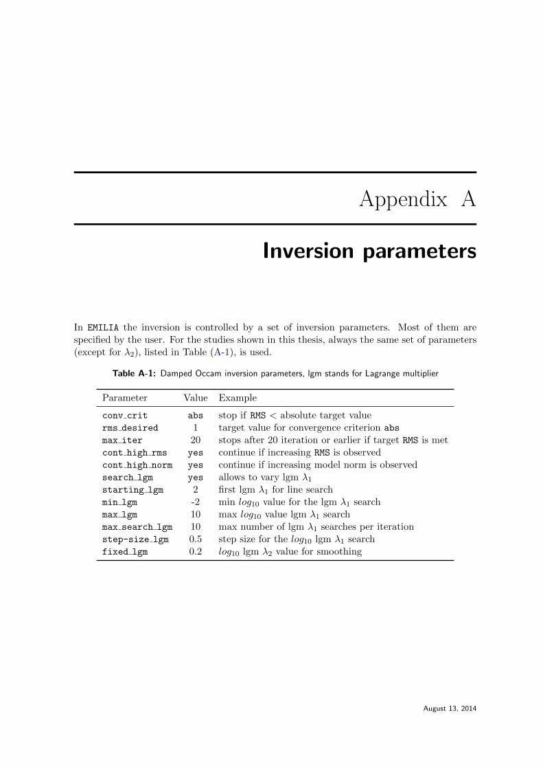
Appendix A
Inversion parameters
In EMILIA the inversion is controlled by a set of inversion parameters. Most of them arespecified by the user. For the studies shown in this thesis, always the same set of parameters(except for λ2), listed in Table (A-1), is used.
Table A-1: Damped Occam inversion parameters, lgm stands for Lagrange multiplier
Parameter Value Example
conv crit abs stop if RMS < absolute target valuerms desired 1 target value for convergence criterion abs
max iter 20 stops after 20 iteration or earlier if target RMS is metcont high rms yes continue if increasing RMS is observedcont high norm yes continue if increasing model norm is observedsearch lgm yes allows to vary lgm λ1
starting lgm 2 first lgm λ1 for line searchmin lgm -2 min log10 value for the lgm λ1 searchmax lgm 10 max log10 value lgm λ1 searchmax search lgm 10 max number of lgm λ1 searches per iterationstep-size lgm 0.5 step size for the log10 lgm λ1 searchfixed lgm 0.2 log10 lgm λ2 value for smoothing
August 13, 2014
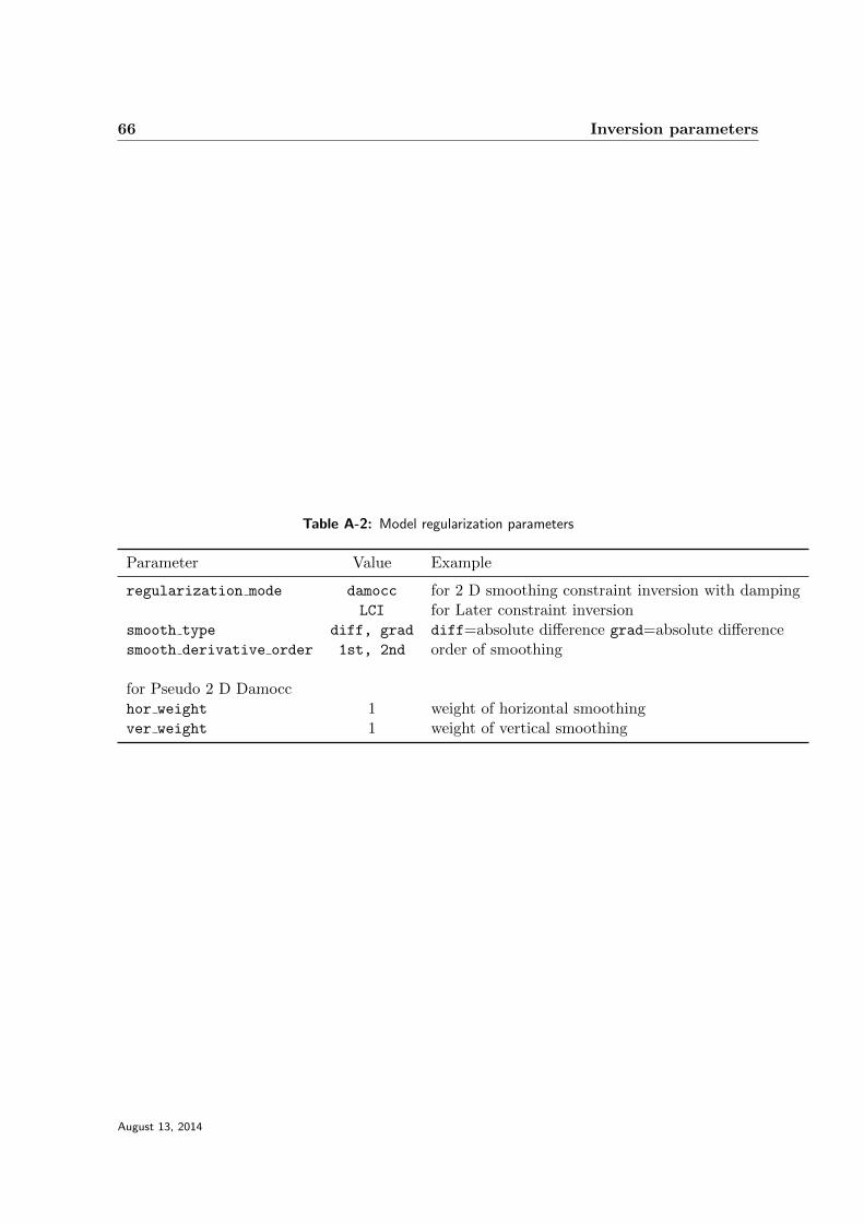
66 Inversion parameters
Table A-2: Model regularization parameters
Parameter Value Example
regularization mode damocc for 2 D smoothing constraint inversion with dampingLCI for Later constraint inversion
smooth type diff, grad diff=absolute difference grad=absolute differencesmooth derivative order 1st, 2nd order of smoothing
for Pseudo 2 D Damocchor weight 1 weight of horizontal smoothingver weight 1 weight of vertical smoothing
August 13, 2014
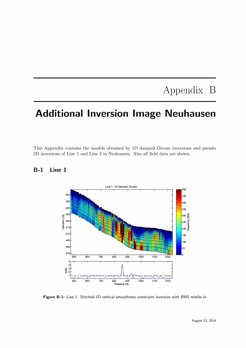
Appendix B
Additional Inversion Image Neuhausen
This Appendix contains the models obtained by 1D damped Occam inversions and pseudo2D inversions of Line 1 and Line 3 in Neuhausen. Also all field data are shown.
B-1 Line 1
Figure B-1: Line 1: Stitched 1D vertical smoothness constraint inversion with RMS misfits in
August 13, 2014
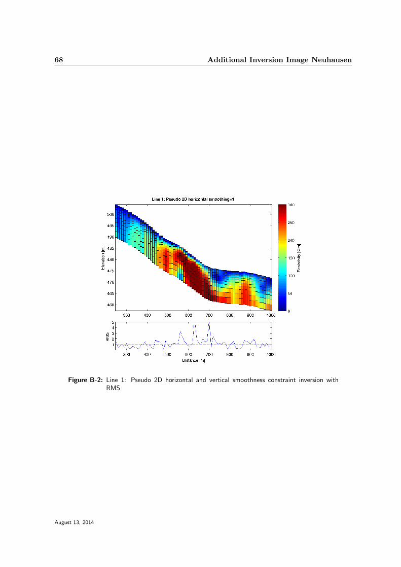
68 Additional Inversion Image Neuhausen
Figure B-2: Line 1: Pseudo 2D horizontal and vertical smoothness constraint inversion withRMS
August 13, 2014
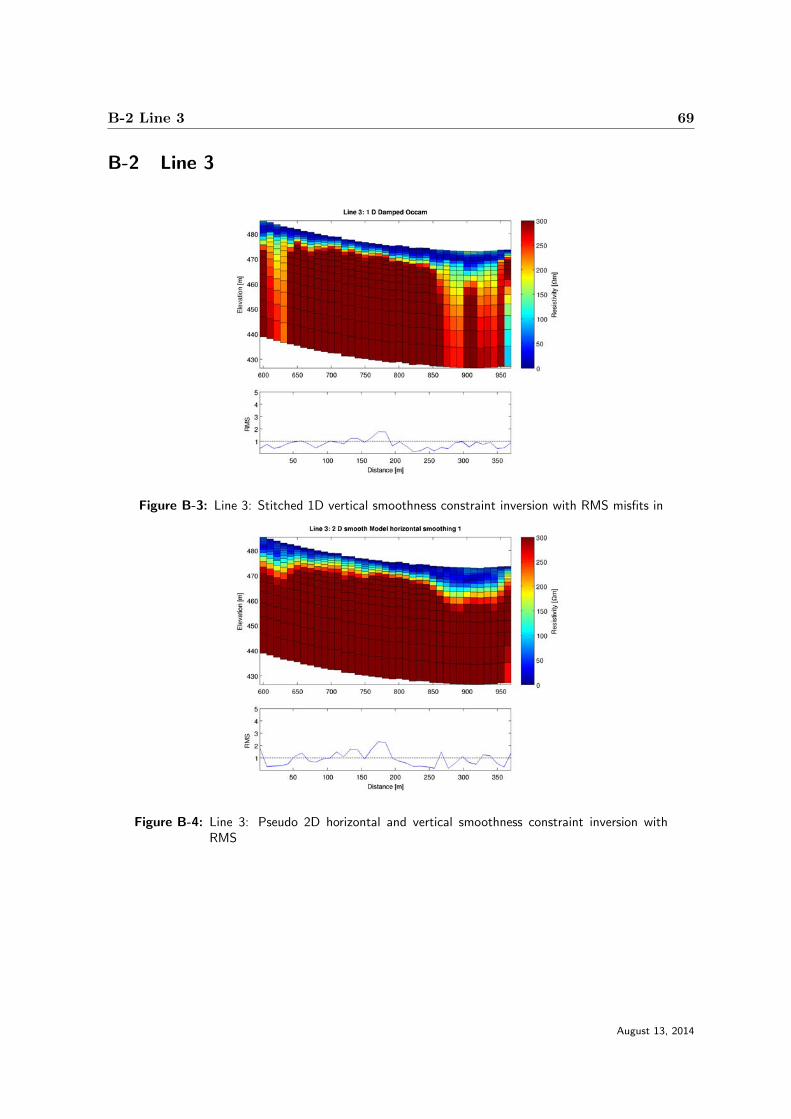
B-2 Line 3 69
B-2 Line 3
Figure B-3: Line 3: Stitched 1D vertical smoothness constraint inversion with RMS misfits in
Figure B-4: Line 3: Pseudo 2D horizontal and vertical smoothness constraint inversion withRMS
August 13, 2014
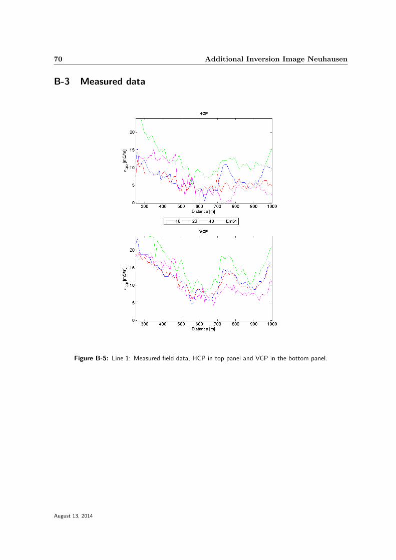
70 Additional Inversion Image Neuhausen
B-3 Measured data
Figure B-5: Line 1: Measured field data, HCP in top panel and VCP in the bottom panel.
August 13, 2014
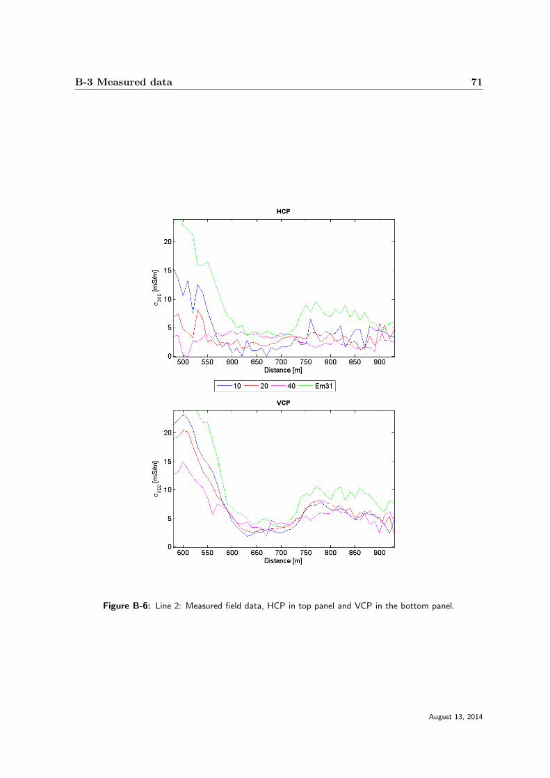
B-3 Measured data 71
Figure B-6: Line 2: Measured field data, HCP in top panel and VCP in the bottom panel.
August 13, 2014
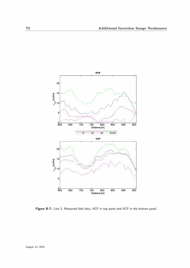
72 Additional Inversion Image Neuhausen
Figure B-7: Line 3: Measured field data, HCP in top panel and VCP in the bottom panel.
August 13, 2014

Appendix C
Additional Inversion Image Ice Ridge
This Appendix contains the models obtained by 1D Marquardt-Levenberg inversions and LCIinversions of Line 0 and Line 1 . Also all field data are shown.
C-1 Line 0
Figure C-1: Line 0: Stitched 1D inversions vertical smoothness constraint; RMS misfits in the
August 13, 2014

74 Additional Inversion Image Ice Ridge
Figure C-2: Line 0: 1D Marquardt-Levenberg inversions a) 2-layer models and b) 3-layer withRMS at the bottom. For better visualizations the GPS heights shown at the top.
August 13, 2014
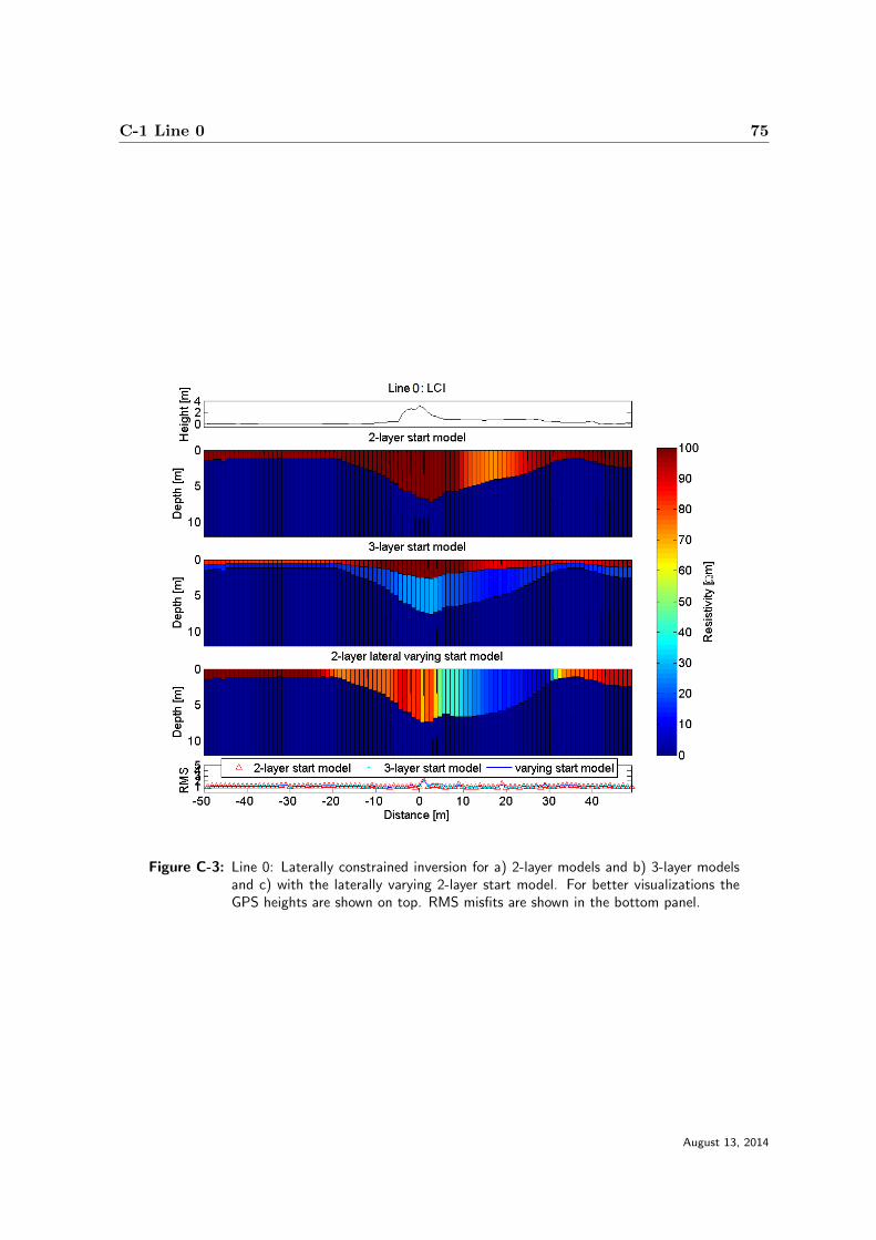
C-1 Line 0 75
Figure C-3: Line 0: Laterally constrained inversion for a) 2-layer models and b) 3-layer modelsand c) with the laterally varying 2-layer start model. For better visualizations theGPS heights are shown on top. RMS misfits are shown in the bottom panel.
August 13, 2014

76 Additional Inversion Image Ice Ridge
C-2 Line 2
Figure C-4: Line 2:1D Marquardt-Levenberg inversions a) 2-layer models and b) 3-layer withRMS at the bottom. For better visualizations the GPS heights shown at the top
August 13, 2014

C-2 Line 2 77
Figure C-5: Line 2:Laterally constrained inversion for a) 2-layer models and b) 3-layer modelsand c) with the laterally varying 2-layer start model. For better visualizations theGPS heights are shown on top. RMS misfits are shown in the bottom panel.
August 13, 2014

78 Additional Inversion Image Ice Ridge
C-3 Measured Data
Figure C-6: a) Horizontal coplanar (HCP) GEM-2 and b) Vertical coplanar (VCP) data of ridgeat line 0 x=0m.
August 13, 2014

C-3 Measured Data 79
Figure C-7: a) Horizontal coplanar (HCP) GEM-2 and b) Vertical coplanar (VCP) data of ridgeat line 1 x=10m.
August 13, 2014
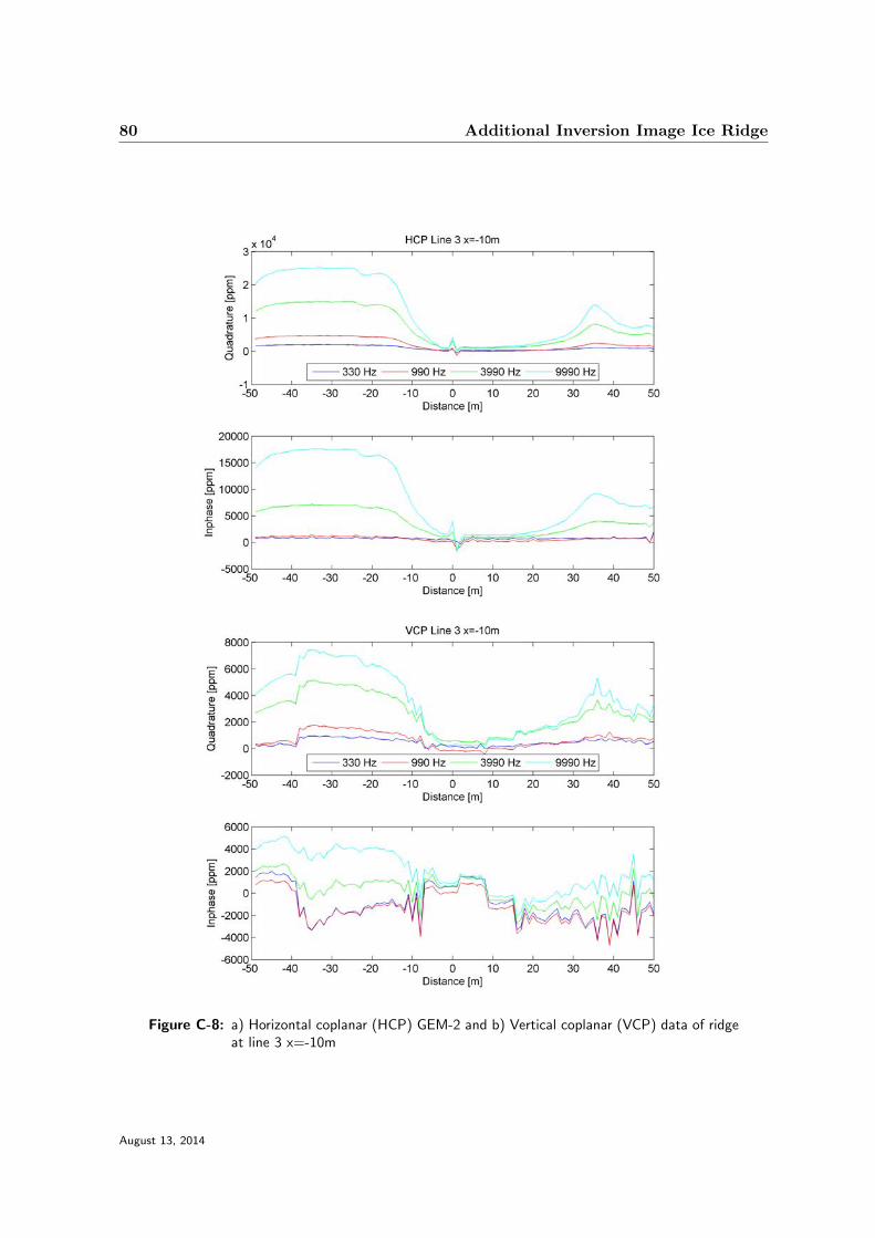
80 Additional Inversion Image Ice Ridge
Figure C-8: a) Horizontal coplanar (HCP) GEM-2 and b) Vertical coplanar (VCP) data of ridgeat line 3 x=-10m
August 13, 2014