Embed Size (px)
Citation preview
THE ROLE OF AGRICULTURAL INPUT SUBSIDY PROGRAMME IN RURAL
POVERTY REDUCTION: INDIVIDUAL HOUSEHOLD MODELING
APPROACH
Master of Arts (Economics) Thesis
By
NICKSON ERIC KAMANGA
BSoc Sc (Mlw)
Submitted to the Faculty of Social Sciences at Chancellor College,
University of Malawi, in partial fulfillment of the requirements for a Master
of Arts Degree in Economics
August, 2010
ii
Declaration
I hereby declare that this thesis is my own work and that it has never been submitted for
similar purposes, to any university or institution of higher learning. Acknowledgements
have been duly made where other people’s work has been used. I am solely responsible
for all errors that this document contains.
Candidate:______________________________________________________________
Date:___________________________________________________________________
iii
STATEMENT OF APPROVAL
This thesis has been submitted with our approval.
Supervisor:______________________________________________________________
Dr. Levison Chiwaula
Date:___________________________________________________________________
Supervisor:______________________________________________________________
Dr. Spy Munthali
Date:___________________________________________________________________
iv
TABLE OF CONTENTS
Declaration......................................................................................................................... ii
Statement of Approval ..................................................................................................... iii
Table of Contents ............................................................................................................. iv
List of Tables .................................................................................................................. viii
Liist of Figures.................................................................................................................. ix
List of Acronyms ................................................................................................................x
Dedications........................................................................................................................ xi
Abstract ........................................................................................................................... xiii
CHAPTER ONE ................................................................................................................1
Introduction ........................................................................................................................1
1.1 Background ....................................................................................................................1
1.2 Statement of the Problem ...............................................................................................3
1.3 Significance of the Study ...............................................................................................5
1.4 Study Objectives ............................................................................................................6
1.5 Hypotheses Tested .........................................................................................................6
1.6 Organization of the Thesis .............................................................................................6
v
CHAPTER 2 .......................................................................................................................7
History of Agicultual Input Subsidies in Malawi ............................................................7
2.1 Introduction ....................................................................................................................7
2.2 From 1952 to Early 1980s: The Era of Universal Input Subsidies ................................7
2.3 Structural Adjustment Policies and Removal of the Universal Input Subsidies ............8
2.4 Starter Pack and Targeted Input Programs ....................................................................9
2.5 Agricultural Input Subsidy Program ............................................................................10
CHAPTER 3 .....................................................................................................................11
Literature Review ............................................................................................................11
3.1 Introduction ..................................................................................................................11
3.2 Theoretical Literature ...................................................................................................11
3.2.1 The Contending Schools of Thought Concerning Government Intervention ...........11
3.1.2 Efficiency Considerations .........................................................................................16
3.2.3 Equity Considerations ...............................................................................................18
3.2.4 Externality Considerations ........................................................................................19
3.1.5 Linkage between Agriculture and Poverty Reduction ..............................................20
3.3 Empirical Literature .....................................................................................................22
vi
CHAPTER 4 .....................................................................................................................26
Methodology and Data Analysis .....................................................................................26
4.1 Introduction ..................................................................................................................26
4.2 Data Collection ............................................................................................................26
4.3 Conceptual Framework ................................................................................................27
4.4 Counter-factual ............................................................................................................28
4.5 Confounding Factors ....................................................................................................29
4.6 Analytical Framework .................................................................................................29
4.7 Simulation ....................................................................................................................31
4.7.1 Two Hundred and Fifty Percent (250%) Maize Price Increase ................................31
4.7.2 One Hundred Percent (100%) Coverage of the Village with Subsidized Fertilizer .31
4.8 Some Methodological Issues .......................................................................................32
CHAPTER 5 .....................................................................................................................34
Results and Interpretation ..............................................................................................34
5.1 Introduction ..................................................................................................................34
5.2 Demographic Characteristics .......................................................................................34
5.3 Household Assets .........................................................................................................35
vii
5.4 Household Income Sources..........................................................................................36
5.5 Household Disposable Income ....................................................................................37
5.6 Distribution of the Subsidized Fertilizer in the Village ...............................................39
5.7 Confounding Factors ....................................................................................................41
5.8 Impact of the Agricultural Input Subsidy on the Poverty Profile ................................42
5.9 Simulations ..................................................................................................................46
5.9.1 Scenario I: A 250% Increase in the Price of Maize ..................................................46
5.8.2 Scenario II: 100% Coverage of the Village with the Input Subsidy Programme .....49
CHAPTER 6 .....................................................................................................................51
Conclusion and Policy Recommendations .....................................................................51
6.1 Summary ......................................................................................................................51
6.2 Policy Recommendations.............................................................................................52
6.3 Limitations ...................................................................................................................54
6.4 Direction for Future Research ......................................................................................54
References .........................................................................................................................55
Appendices ..........................................................................................................................1
viii
List of Tables
Table 1: Summary statistics for demographic variables .................................................. 35
Table 2 Average Dependency ratio, Age and Household income by income quintile ...... 35
Table 3: Household Asset Holding by Type and Income Quintile .................................... 35
Table 4: Percentage distribution of income from different sources by income quintile ... 37
Table 5: Distribution of upland maize farms and average yield per acre between
households that received fertilizer and those that did not ................................................ 41
Table 6: Distribution of average income per household from other intervention in the
village ................................................................................................................................ 41
ix
List of Figures
Figure 1: Population Pyramid ........................................................................................... 34
Figure 2: Percentage contribution of different sources to total village income ................ 36
Figure 3: Contribution of different income sources to household income ....................... 37
Figure 4: Household Disposable income per adult equivalent showing households below
the "food requirement" threshold ...................................................................................... 38
Figure 5: Household disposable income per adult equivalent showing households below
and above the SOLT ......................................................................................................... 39
Figure 6: Household disposable income per adult equivalent showing households
benefited and those that did not benefit from the AISP .................................................... 40
Figure 7: Net returns per adult equivalent from maize production ................................... 42
Figure 8: Disposable income per adult equivalent with and without the subsidized
fertilizer ............................................................................................................................. 43
Figure 9: Disposable income per adult equivalent without the subsidy showing the initial
income status of the households ....................................................................................... 44
Figure 10: Disposable income per adult equivalent showing households below and above
the food and SOLT thresholds without the impact of the subsidy .................................... 45
Figure 11: Comparison of DY/AE before and after a 250% rise of maize price .............. 47
Figure 12: DY/AE showing households below and above the food and SOLT after the
price rise ............................................................................................................................ 48
Figure 13: Comparison between survey values and 100% coverage values of DY/AE ... 49
Figure 14: Welfare impact of 100% coverage of the village ............................................ 50
x
List of Acronyms
ADMARC Agricultural Development and Marketing Corporation
AERC African Economic Research Consortium
AISP Agricultural Input Subsidy Programme
DY/AE Disposable income per adult equivalent
GDP Gross Domestic Product
GoM Government of Malawi
HEA Household Economy Approach
IHMA Individual Household Modeling Approach
IHS Integrated Household Survey
Kg Kilogram
MARDEF Malawi Rural Development and Entrepreneurship Fund
MASAF Malawi Social Action Fund
MDGs Millennium Development Goals
MGDS Malawi Growth and Development Strategy
MPRSP Malawi Poverty Reduction Strategy Paper
MT Metric tonnes
ODI Overseas Development Institute
PAP Poverty Alleviation Programme
PRSPs Poverty Reduction Strategy Papers
PWP Public Works Programme
SAPs Structural Adjustment Policies
SOLT Standard of Living Threshold
SSA Sub-Saharan Africa
TIP Targeted Input Programme
Dedications
To my loving wife Anna Scevah, thank you for your encouragement and support. To my
daughter and great friend, Emma. I understand why you did not understand why dad had
to go away. To my sons, Nick Jr., Jack, Paul, Noah and Eric Jr. and daughter, Etta.
To my mom, Etta Nya Mumba.
For a testimony to the faithfulness of the Lord.

ACKNOWLEDGEMENTS
I wish to express my sincere gratitude to my Supervisors Dr. Levison Chiwaula and Dr.
Spy Munthali for their patience and untiring efforts in providing guidance during the
writing of this thesis. Your constructive comments made this daunting task much more
bearable.
I would also like to thank the Department of Economics for offering me the opportunity
to undertake the post-graduate training by providing material support. I also acknowledge
all the members of staff in the Department of Economics for the countless hours they
have dedicated to my training and education, for their approachability and for providing
moral support.
I am also very grateful to the Evidence for Development and African Economic Research
Consortium (AERC) who separately provided financial support which enabled my
participation in Master of Arts programme in Economics in Malawi and Kenya
respectively.
Special thanks are due to Dr John Seaman and Dr. Celia Petty of the Evidence for
Development, for their inclusion of me in the Individual Household Modeling Approach
(IHM) Project, thus enabling me to use the methodology in this manuscript. Thanks also
go to Dr. Patrick Kambewa who facilitated my interactions with the Evidence for
Development and demonstrated how to conduct fieldwork.
My acknowledgements will be incomplete without thanking and appreciating the help
and guidance offered by all classmates especially Frederick and Edith and Lauryn and
Mulenga. You gave me hope.
Finally, I thank the residents of the sample villages for their patience and hospitality as I
conducted my research.
ABSTRACT
This study investigates the role of Agricultural Input Subsidy Programme on poverty
reduction in rural Malawi using the Individual Household Modeling Approach. The study
is based on information derived from a village in Chingale area in Zomba District. Using
a “with” and “without” the subsidy project evaluation approach, the study makes a
comparison of the ultra poverty and poverty rates in the two scenarios. The Agriculture
Input Subsidy Programme has a positive impact on the poverty rate. However, the
programme does not affect the proportion of households living below food security
threshold. The poorest of the poor are not made any better off as a result of the AISP. The
implication is that on average, the food security situation of the lowest income group is
not improved by the subsidy programme. Moreover, the maize price escalations that
occur during the traditional lean months of December to February implies worsening
food security situation for all maize deficit households and more so for the ultra poor
since it usually means surviving on less than the required kilocalorie intake. However,
complete coverage of smallholder households with one 50kg bag of fertilizer is expected
to greatly reduce both the poverty and ultra poverty rates.
The study also examines the targeting efficiency of the AISP and finds that the
programme is biased towards the richer households. Although this conforms to the
programme’s design structure, it is also a constraining factor to the programme’s
effectiveness as a social safety net tool.
CHAPTER ONE
INTRODUCTION
1.1 Background
Poverty in Africa and in the Sub-Saharan Africa (SSA) in particular, has remained
constant over the last two decades. For instance, between 1981 and 2005, the poverty rate
in the SSA has shown no sustained decline in that it remained at around 50%. In absolute
terms, the number nearly doubled from 200 to 380 million people. Over the same period,
poverty had been declining elsewhere in the developing world (World Bank, 2008)
Concerned with the uneven progress of development, the United Nations designed new
poverty reduction interventions known as the Millennium Development Goals (MDGs) in
the year 2000. The MDGs are a set of eight goals for which eighteen numerical targets
have been set and about forty quantifiable indicators have been identified. To show its
seriousness to poverty issues, the first goal of the MDGs calls for the eradication of
poverty and extreme hunger (World Bank, 2008). Precisely; this goal has two specific
targets namely: to halve between 1990 and 2015, the proportion of people under the
poverty line as well as the proportion of people who suffer from hunger (World Bank,
2010).
To enable the developing countries to achieve the Millennium Development Goals, the
international donor community complements individual governments’ efforts within the
Poverty Reduction Strategy Papers (PRSPs) framework. That is, governments are
required to prepare policy documents (PRSPs) which form the basis for negotiations with
the donor community on General Budget Support. The overall goal of the PRSPs is
poverty reduction through empowerment of the poor.
Malawi has demonstrated concerted effort to fight poverty within the confines of the
MDGs, using both policy instruments and targeted interventions to the poor or vulnerable
sectors of society. For instance, the government launched the Poverty Alleviation
Program (PAP) in 1994 which was aimed at fighting rampant poverty in Malawi
(AFRODAD, 2005). The PAP framework laid out four specific objectives namely, to
raise the productivity of the poor, to promote sustainable poverty reduction, to enhance
participation of the poor in the social economic development process so as to raise and
uphold individual and community self esteem, and to increase income and employment
opportunities for the poor.
The PAP was followed by the launch of the Malawi Social Action Fund (MASAF) in
1995 to provide targeted assistance to the chronically poor and finance community driven
development. A key component of MASAF was Public Works Programme (PWP) in
food deficit areas involving self-targeting food and cash for work (Devereux, 1997). At a
later stage, a revolving credit facility named Malawi Rural Development and
Entrepreneurship Fund (MARDEF) was added to MASAF. The PAP lacked effective
implementation mechanism (AFRODAD, 2002), as a result it was replaced by the
Malawi Poverty Reduction Strategy Paper (MPRSP) as the country’s growth strategy.
The MPRSP was launched in 2002. The overall goal is poverty reduction through
empowerment of the poor to be pursued through interventions in rural infrastructure
development, human capital development, provision of social safety nets to the
vulnerable and good governance (GoM, 2002). The MPRS tended to be biased toward
public spending with insufficient treatment of rural productive sectors and failure to
explore their potential contribution to pro-poor growth (Rakner et al, 2004). In 2005 the
government therefore began developing its second generation PRSP known as the
Malawi Growth and Development Strategies (MDGS). MGDS’ objective is to reduce
poverty through sustained economic growth and infrastructure development, particularly
in rural areas through the development of rural growth centers. One of the key areas the
MDGS focuses on is agriculture and food security (GoM, 2007).
Nonetheless, despite the determined efforts to eradicate or alleviate poverty, poverty in
Malawi still remains high and was last estimated at 52.4%, of which 22.2% lived in ultra
poverty (GoM, 2005). The Integrated Household Survey (IHS) of 2005 also indicates that
of the 85% of the population that constitute rural smallholder farmers, 58% of these earn
their income from the sale of crops. Hence, interventions that aim to enhance agricultural
productivity of the cash constrained, poor rural households by giving them free
agricultural inputs can have widespread positive impacts on people’s welfare.
Conversely, a decline in the agricultural sector has serious consequences on people’s
welfare. It is on this basis that current agricultural input subsidies have been adopted as
an intervention to promote agricultural growth and to address food security and poverty
alleviation goals. This study therefore attempts to investigate the impact of the fertilizer
subsidies on poverty alleviation among the rural households.
1.2 Statement of the Problem
Since 1994, the Government of Malawi made poverty alleviation a priority concern in its
economic policy. Consequently, many programmes whose objective is to reduce poverty
generally and rural poverty specifically, have been implemented not only by the Malawi
government but also by various bilateral and multilateral donor agencies. Most notable
among such programmes are Malawi Social Action Fund, the Public Works Programme
and the Malawi Social Cash Transfer Programme.
Despite these efforts, poverty in Malawi remains pervasive. The Second Integrated
Household Survey (IHS) report of 2005 indicates a national poverty rate of 52%. This
implies that between 1998 and 2005 the poverty rate only dropped by 2% from 54% as of
1998 (GoM/World Bank 2007). Poverty in Malawi is a predominantly rural phenomenon
because 94% of the poor people live in the rural areas (GoM, 2005). Most of the people
living in the rural areas are smallholder farmers who earn their living through agriculture
since the Malawian economy is agro-based.
Malawian smallholder agriculture is characterized by large numbers of very poor farmers
heavily dependent on low input maize production on small land holdings which are very
short of nitrogen (Dorward et al, 2008). Maize production by these farmers is normally not
sufficient to meet annual consumption needs, and they depend upon casual labouring and
other income earning opportunities to finance the purchase of the balance of their needs.
In the 2002/3 and 2003/4 cropping seasons when the government implemented the Targeted
Input Programme( TIP), around 40% of smallholder households purchased an average of
65kg of fertilizer on commercial terms. (Dorward et al, 2008). These numbers suggest that
more than half of the smallholder population did not afford to purchase adequate
quantities of fertilizer on commercial terms. The implication is that many farmers are
vulnerable to impoverished livelihoods based on low productivity maize cultivation and
casual labouring. Food insecurity problems facing such farmers worsen with national food
shortages due to poor production seasons and late and expensive government-funded
imports leading to large increases in maize purchase prices. In trying to mitigate these
problems, the government started implementing the Agricultural Input Subsidy
Programme (AISP) in the 2005/06 season with the objectives of improving smallholder
productivity and food and cash crop production and reducing vulnerability to food
insecurity and hunger. Other objectives were to promote food self sufficiency,
development of the private sector input markets, and wider growth and development.
The AISP has generated considerable debate in Malawi and internationally. Both sides of
the debate however, agree that the program has significantly improved the national food
security situation in Malawi. Several studies (Dorward et al, 2008; Chirwa, 2007;
Chinsinga and O’Brien, 2008) have confirmed this observation. Other studies have
focused on private sector displacement effect of the subsidy (Dorward et al, 2008,
Ricker-Gilbert and Jayne, 2009) and household food security (Chirwa, 2010). Anecdote
studies on targeting efficiency of the programme also exist (Chinsinga, 2002). There is
however, discernible absence of literature about the impact of the AISP on the income
welfare of the households. This study endeavours to bridge the knowledge gap by
determining whether the agricultural input subsidies have an impact on rural poverty and
also examines the targeting efficiency of the programme. The study utilizes data obtained
through enumeration of a village called Chisanje I located in the Chingale area in Zomba
District. Despite the single village focus of the study, we expect to draw lessons that
apply for the nation. The study uses Individual Household Modeling (IHM) approach for
data analysis.
1.3 Significance of the Study
In the light of the problem articulated in the foregoing section, this study therefore
contributes to understanding the impact of the agricultural input subsidy program on the
welfare of rural households in Malawi. Agricultural input subsidies’ central goal is to
promote adoption of new technologies and thus increase maize production both
nationally and at household level. In a country such as Malawi, with 94% of the poor
residing in rural areas (GoM, 2005), 85-90% of whom work in agriculture mainly as
smallholders who produce maize first and foremost for home consumption (Chirwa,
2010; Harrigan, 2008; Rickert-Gilbert and Jayne, 2009), and with over 80% of food share
in the poverty line (ODI, 2004), there is a close link between food security and poverty.
By increasing maize productivity, agricultural input subsidies address the issue of food
security which is fundamental to rural poverty reduction. Food insecure households are
likely to engage in coping strategies such as ganyu labour and asset depletion which
further intensifies the vicious food insecurity-poverty cycle. Increased maize productivity
on the other hand enables households to produce surplus yields which they sale to meet
other household needs as well as to accumulate assets, and thus enables them to
meaningfully participate in the economic development process.
The significance of the study with respect to policy cannot be overemphasized. Poverty
reduction is at the core of the Millennium Development Goals (MDGs) which inform the
Malawi Growth and Development Strategies (MGDS). Malawi’s pathway to poverty
reduction, as envisaged in the MGDS, involves increased agricultural productivity and
food security as the primary goals of the first key priority area. One of the key strategies
for achieving the goals include providing the means for Malawian’s to gain income and
put in place effective social protection programs with improved targeting (GoM, 2005).
AISP is implemented as part of this strategy. However the direct impact of the strategy on
rural household poverty has not been examined.
1.4 Study Objectives
The main objective of this study is to investigate the impact of the AISP on household
poverty. To achieve this main objective, the study specifically attempts:
1. To determine the impact of the AISP on household incomes.
2. To investigate the household food security impact of the AISP.
3. To examine the extent to which the input subsidy is targeting poor households.
1.5 Hypotheses Tested
Based on the foregoing objectives, the study will test the following null hypotheses:
1. The Agricultural Input Supply Program does not have an impact on household income.
2. The AISP does not contribute to food security of households.
3. The AISP is not efficiently targeted
1.6 Organization of the Thesis
Chapter Two is devoted to background information. It gives the history of input subsidies
in Malawi and also describes the poverty situation in Malawi between 1998 and 2005. It
then analyzes the economic environment in Malawi from 1994 to 2007. Chapter Three
reviews the literature. It starts by exploring two contending schools of thought regarding
government intervention in the market and then shows the link between agricultural
development and poverty reduction. It then reviews other papers that have attempted to
assess the impact of subsidies in Malawi and elsewhere.
Chapter Four describes the methodologies used in this study while Chapter Five is
devoted to the presentation and discussion of results. Chapter Six winds up by drawing
conclusions and policy implications based on the results and discussions.
CHAPTER 2
HISTORY OF AGRICULTURAL INPUT SUBSIDIES IN MALAWI
2.1 Introduction
The agricultural sector is the single most important sector of the Malawi economy. At
independence, the Malawi economy was predominantly agricultural, with the agricultural
sector accounting for 55% of the gross domestic product (GDP) and 90% of domestic
employment (McCracken, 1983). Agriculture continues to be a significant driver of
economic growth, accounting for 38% of the Malawi economy’s GDP, 80% of its export
earnings and supports 85% of the population (World Bank, 2009).
2.2 From 1952 to Early 1980s: The Era of Universal Input Subsidies
Due to its strategic importance to the Malawi economy, the agricultural sector has
benefited from subsidies practically for most of Malawi’s modern history, having been
introduced in 1952. The objective of the subsidies in colonial Malawi was to ensure the
distribution of vital agricultural inputs at a low cost to even the most geographically
remote smallholder farmers and the goals were to increase maize productivity and
maintain soil fertility. Post Colonial government’s involvement in agricultural sector was
widespread. Apart from promoting an agricultural-based export-oriented development
strategy, government placed national food security high on its domestic policy. The
national food security goal was achieved via emphasis on smallholder production of
maize. The strategy received strong support from the state through the state marketing
board, Agricultural Development and Marketing Corporation (ADMARC), which offered
smallholder farmers, subsidized maize seed and fertilizer and purchased the maize output
at guaranteed pan territorial prices. ADMARC also sold the maize in the domestic market
at subsidized consumer prices (Harrigan, 2008)
Although the strategy succeeded in achieving national aggregate food security, individual
household food security was not guaranteed because of conflicting policy objectives
which favoured the estate sector (Harrigan, 1988) and led to the impoverishment of the
smallholder sector.
2.3 Structural Adjustment Policies and Removal of the Universal Input Subsidies
By late 1970s, Malawi suffered the impact of a series of exogenous shocks such as the
dramatic deterioration in the terms of trade; a sharp rise in international interest rate;
drought conditions in 1979-80 (Mosley et al, 1991); and disruption of Malawi’s
traditional trade route to the sea due to the civil war in Mozambique. Government’s
budgetary position worsened and this was aggravated by financial deterioration
experienced by ten major parastatal companies which were operating at a loss from 1977
onwards (Mosley et al, 1991).
These conditions underscored the need for a reorientation of agricultural policy in
Malawi under the auspices of the World Bank and International Monetary Fund structural
adjustment and stabilization programmes (SAPs). Liberalization of the agricultural sector
led to increased ADMARC producer prices for smallholder export crops while the
producer price of maize was reduced. Simultaneously, Malawi liberalized the agricultural
input markets and started phasing out subsidies on smallholder fertilizer and seed
(Mosley, 1991; Harrigan, 2008). By 1996, government had completely removed the
universal fertilizer subsidy. The objective was to remove price distortions and increase
the smallholder contribution to export earns.
Consequently, the cost of agricultural inputs increased dramatically, making fertilizer
unaffordable to most smallholder farmers. Smallholder fertilizer uptake declined in
absolute terms as a consequence of the price increase and the collapse of the Smallholder
Credit Administration. With the collapse of the formal marketing system in 1985-6, many
risk-averse farmers shifted their cash cropping pattern out of improved maize and
towards groundnuts which enjoyed well developed informal markets. By the 1990s, both
household and national food security had become more precarious in Malawi (Chilowa,
1998; Sahn et al, 1990) and poverty had increased. Rural livelihoods were deteriorating
(Frankenberger, et al, 2003) and inequality among smallholders had increased (Peters,
1996). In addition, the effect of market liberalization and the reduced role of ADMARC
in the maize market were such that the intra-seasonal maize consumer price widened.
This adversely affected rural households’ food security, 80% of which had become net
purchases of maize (Hamington, 2001).
2.4 Starter Pack and Targeted Input Programs
The Starter Pack Programme was launched in 1998 in response to the growing evidence
of catastrophic decline in soil fertility and maize productivity (Harrigan, 2008). The
program was intended to meet several objectives including increasing maize yields and
food security, countering soil nutrient depletion, and making a new line of fertilizer-
responsive semi-flint hybrids available to small farmers who otherwise would not take
the risk to experiment with them. The program was designed to provide all smallholders
with small packages containing semi flint hybrid (2kg) and fertilizer (15kg) as well as
legumes (1kg of seed) to improve soil fertility. The pack was enough to cultivate about
0.1 hectares of farm size and it was estimated that that farmers would be able to produce
an extra 100-150kg of maize.
In terms of coverage, it extended to all rural farming households and was repeated in the
1999/2000 growing season. With the assistance of good weather, smallholder maize
production registered a record 2.5 million tons which was 1.0 million tons higher than the
long term average production and 500 thousand tons higher than the previous record of
1993 (Crawford et al, 2005; Harrigan, 2008; Dorward, 2009; Gilbert and Jayne, 2009).
The programme thus improved households’ food security and income position (Cromwell
et al, 2001, Oygard et al, 2003) via two channels. Firstly it provided an extra 2 to 2.5
months of maize cover for an average household of six members. The second channel
worked through the market mechanism since the increased household maize production
reduced demand for maize in the market and hence dampened the intra-seasonal increase
in the maize consumer price. This further lessened the crowding out of the chronically
poor households by the better off in the maize market (Harrigan, 2008). The Starter Pack
thus contributed to poverty alleviation particularly in the early years when nearly all rural
households were beneficiaries (Crawford et al, 2006).
2.5 Agricultural Input Subsidy Program
Another acute hunger crisis repeated in the 2004/05 growing seasons, which affected five
million people and forced the government into a costly exercise of importing emergency
food. Consequently government deepened fertilizer subsidies by introducing a large-scale
input subsidy, the Agricultural Input Subsidy Program in the 2005/06 growing season.
The objective was to promote access to and use of fertilizer in both maize and tobacco
production in order to increase agricultural productivity and food security (Mann, 2003;
Dorward, et al. 2008). The programme was particularly intended to improve land and
labour productivity and production of both food and cash crops by smallholder farmers
that faced heavy cash constraints restraining them from purchasing the necessary inputs
(Dorward, et al. 2008). The overall goal was to promote economic growth and reduce
vulnerability to food insecurity, hunger, and poverty.
The program was implemented through the distribution of coupons for four types of
fertilizer which recipients could redeem at parastatal outlets at approximately one third of
the normal cash price. In the first year, 50% of farming households were provided with
2.8 million vouchers for 100kg of fertilizer and a small quantity of maize seed. However,
the programme left out the poorest farm households since it was felt that 100kg of
fertilizer was too much to be used effectively on the small land holdings typical of such
households.
The result was increased national maize output (MT 2.6 million) in the 2005/06 season
while in the 2006/07 growing season the surplus was recorded at 1.3 million metric tons
(Chinsinga, 2002). At household level, the programme improved food security and
lowered the food prices than would have prevailed without the subsidy.

CHAPTER 3
LITERATURE REVIEW
3.1 Introduction
The objective of this chapter is to review literature with respect to agricultural input
subsidies. We first discuss the two major contending schools of thought concerning the
role of government in a free market economy and the objectives behind governments’
adoption of input subsidies. Then we explore the link between agricultural growth and
poverty. The chapter closes with a review of various papers on the impacts of subsidies.
3.2 Theoretical Literature
3.2.1 The Contending Schools of Thought Concerning Government Intervention
Classical welfare economics is premised on Adam Smith’s dictum that each individual, in
pursuit of his own self-interest, is led as if by an “invisible hand” to a course of action
that promotes the general welfare of all. His axiom has been formulated into two
Fundamental Theorems of Welfare Economics. The first theorem states that a perfectly
competitive market economy leads to a Pareto optimum1 allocation of resources provided
certain conditions are met (Weimer and Vining, 2005). The theorem implies that the
market economy will, under certain conditions, lead to efficiency.
Perfect competition in all markets is therefore the benchmark that will lead to a position
of Pareto optimality, given the assumptions that underlay the analysis. These conditions
include availability of: producers and consumers as rational agents who maximize
benefits and minimize costs; a complete set of markets with well defined and costless
enforced property rights; many buyers and sellers who are passive price takers; and zero
transaction costs. Under these conditions, a set of prices arise that allocates resources
Pareto optimally. Pareto efficiency however, depends on the initial endowments of
1 An allocation is said to be Pareto optimal or efficient when every reallocation that augments the utility of
one individual necessarily reduces the utility of another (Gould and Ferguson, 1980)
resources to individuals. If the initial distribution of endowments was not equitable, then
the second theorem applies. It states that after a suitable redistribution of initial wealth,
any desired Pareto-efficient allocation of resources can be achieved by a perfectly
competitive economy, provided certain conditions are met. The second theorem claims
that under those conditions, the market economy will lead to an outcome that is both
efficient and equitable.
Using the Marshalling demand, such a competitive market economy has a tendency to
converge towards a general equilibrium in sense that the quantity demanded exactly
equals the quantity supplied. The equilibrium is Pareto optimal in that it also maximizes
social surplus2 and is characterized by zero economic rent
3 as long as entry into the
industry is free. Therefore, policy interventions that move prices away from the
equilibrium price and quantity lead to inefficiencies through loss of social surplus.
However, there are instances when perfect competition does not lead to maximum social
welfare due to existence of external economies4. Coase (1937), argued that even in these
cases, a perfectly competitive economy would still achieve a socially optimal level of
output without government interventions through taxes or subsidies. Assuming that the
income effects and transaction costs were negligible, voluntary contracts among the
different parties concerned would lead to a socially optimal output even in the presence
of externalities. He further argued that the result would be the same regardless of which
party is assigned the property rights to the contestable resource.
According to this theory, a farmer is motivated by profit in his pursuit of self interest and
would therefore demand the amount of fertilizer that maximizes financial returns (Shultz,
2 Net benefits consumers and producers receive from participation in the market or the sum of consumer
surplus and producer surplus.
3 That is, total revenue minus payments at competitive market prices to all factors of production, including
an implicit rental price for capital owned by the firm.
4 An external economy (diseconomy) is said to exist when marginal social cost is less than (greater than)
marginal social benefit (Gould and Ferguson, 1980).
1964). This amount is determined by the intersection of the farmer’s effective demand
for, and firms’ supply curve of fertilizer (Ellis, 1992). At the point of intersection, the
farmer’s marginal cost of the last unit of fertilizer applied is equal to the value of the
marginal benefit.
Accordingly, fertilizer subsidies should be discouraged because the distortions they
induce have consequences for the economy (Shultz, 1964) especially if the distribution
function is not function well. For instance, they distort resource allocation at the farm
level to the extent that they encourage farmers to use excessive amounts of fertilizer
beyond profit maximizing levels (Ellis, 1992); they may be hard to target and go to well-
off farmers or those with high cash income (Donovan, 2004; Kherallah, et al, 2002), in
which case they may be regressive as they may displace unsubsidized sales; price control
and rationing may encourage rent seeking behaviour (Ellis, 1992).
Despite its sound economic argument, the profit maximization goal does not augur well
with the smallholder situation due to the dual role of maize in rural Malawi economies.
Malawian smallholder production is food security driven; only surplus production is sold
on the market. Maize is rarely grown for sale and smallholder farmers do not reason in
terms of price signals and profit margins (Donge et al, 2001). Smallholder maize
production decisions are about maximizing output given the constraints of land, labour
and inputs. Moreover, before the introduction of the AISP, 60% of the smallholders did
not purchase any fertilizer (Buffie and Atolia, 2009). In addition, although smallholders
know that correct application of the input greatly increases maize yields, current fertilizer
intensity in Malawi, estimated at 34kg per hectare against the recommended 150kg per
hectare, is very low to achieve food security. Therefore, rather than encouraging
excessive use of fertilizer, provision of subsidized fertilizer in Malawi encourages
fertilizer consumption towards the socially optimal level (Pender et al, 2004), improves
efficiency and enhances food security for the poor (Buffie and Atolia, 2009). In this case
therefore, subsidies do not distort the allocation of resources.
The other school of thought consists of two theories, Economic Theory of Regulation and
the Public Interest Theory, which argue for government intervention in markets. The
economic theory of regulation (Stigler, 1975; Peltzman, 1976) treats regulation like an
ordinary good whose equilibrium price and output are determined by the intersection of
the demand for and supply of regulation. Regulation, such as provision of subsidies and
restriction of entry by rivals, results in the transfer of wealth from government to some
producers and interest groups. The price of this commodity (wealth) takes the form of
open bribes, campaign contributions, and lucrative jobs for relatives of politicians. The
demanders are a small, controllable group of firms or other interest groups while the
suppliers are political regulators who wish to maximize votes and hence ensure security
of tenure.
State legitimacy in Malawi is closely linked to the availability of maize or more broadly,
food security (Chinsinga, 2007, Sahley et al, 2005). The closer the state legitimacy is
linked to maize availability, the more likely food security policy will be politicized and
therefore jeopardizing maize availability and affordability puts at risk the ship of the
state. Consequently, the issue of food security in Malawi has been used to build wider
support for a party or to bolster support for a government (Sahley et al, 2005).
The public interest theory on the other hand is premised on the argument the market
mechanism plays a vital role in the optimal allocation of resources. Market failures are
however, inevitable because the assumptions of the competitive model do rarely conform
to the real world situation and are in practice violated. The violation of the assumptions
produces Pareto optimally inefficient outcomes that do not maximize welfare.
Traditional reasons that account for market failure include the existence of: public goods,
externalities, information asymmetry, and technical externalities. The major reason that
account for market failure in the Malawi rural economy is existence of thin maize input,
output and financial markets which require high risk premiums and margins in order to
make it profitable to engage in such markets. The high margins however, depress
effective demand and thus result in a low level equilibrium trap and hence market failure
(Dorward et al, 2004).
Government intervention therefore is intended to bring about a more equitable outcome at
a lower cost than the private organizations. Government intervention may take a number
of ways. Pigou (1912) argued that in the presence of externalities, government should
intervene by levying taxes on those imposing external costs and subsidies on those who
contribute external benefits. Subsidies will stimulate production or consumption, while
taxes will limit them. Sometimes the government may intervene by directly providing the
public goods and services such as health and education.
This school of thought argues that because of market failure, farmers may not necessarily
seek to maximize profit from fertilizer use since they may not know the yield response
curve and they face affordability, production or output marketing, constraints (Kelly,
2005). Not surprisingly, most African countries have responded to this suboptimal use of
fertilizer by adopting agricultural input subsidies primarily as a means of promoting the
adoption of new technology among farmers and thus increase agricultural productivity
(Ellis, 1992). Subsidies achieve this by allowing farmers to access purchased fertilizer
and improved seeds at low cost and thus remove the disincentives to technology adoption
(Dorward, 2008). These disincentives stem from risk aversion, cash constraint, and low
expectations of returns from investment in agricultural inputs due to limited information
about input benefits. In the Malawi case for instance, the adoption of the Agricultural
Input Subsidy (AISP) has been justified on the basis that it compensates for incomplete
markets that prevent smallholder farmers from investing in highly profitable green
revolution inputs.
Given market failures that account for low fertilizer use and hence smallholder
productivity in Malawi, government intervention in the market is therefore justifiable.
However, a clear understanding of the rationale underlying government policy objective
is crucial for assessing policy impacts on the population. By adopting the AISP, the
Government of Malawi’s objectives were to increase agricultural productivity, to increase
food security and particularly, to improve land and labour productivity and production of
both food and cash crops by smallholders that are faced by heavy cash constraints
restraining them purchasing the necessary inputs (Dorward et al, 2008). Implied in these
objectives are efficiency, equity and externality considerations.
3.1.2 Efficiency Considerations
Farmers’ use of fertilizer may be suboptimal due to several factors that influence their
adoption and intensity of fertilizer use, such as price factors, lack of information, lack of
liquidity and risk aversion.
Price factors affect profitability of fertilizer use. According to Kelly, (2005), profitability
of fertilizer is directly influenced by fertilizer-yield response (or agronomic response),
and input-output prices. Yield response, defined as kilograms of grain obtained by
applying one kilogram of plant nutrient, is a function of soil characteristics and climatic
factors. If the farmer’s perception of yield response and profitability is substantially
lower than that perceived by researchers, then the difference between potential demand
and effective demand will be wide.
Dorward et al (2008) however contended that the many years of fertilizer subsidies in
Malawi have improved farmers’ perceptions of yield response. However, despite
smallholders’ full awareness of the potential for hybrid seed and fertilizer to increase
their maize production, purchases of both is limited (Dorward et al, 2008). The problem
that still remains is the variability in farmers’ ability to effectively and efficiently use
fertilizer. Kumwenda et al. (1997) however, argue that the variability of the environment
over time and space in Malawi and the other SSA countries contributes to the cost of
developing information about agronomic potential and of transmitting this information to
farmers. The role of input subsidies in such an environment should therefore be to help
especially poorer farmers to learn from experience. In the presence of perfect
information, the decision to adopt fertilizer is determined by the interplay of the
agronomic response and the input-output price ratio. In theory, farmers should adopt
fertilizer use if the marginal agronomic response is greater than the input-output price
ratio.
The input-output price ratio, which indicates the number of kilograms of production a
farmer needs to purchase 1kg of fertilizer, is unfavourable in Malawi, mainly because
maize prices have been highly volatile especially over the last ten years (Minot, 2010).
Volatility is a consequence of thin agricultural markets in the country and the SSA region
generally; (because only a small portion of many crops enter the market) which means
that small changes in total production can result in large proportional changes in
marketed surplus. Output price volatility therefore induces uncertainty and risk5. Risk
associated with fertilizer use in Malawi includes production risk (variability in fertilizer
response) and price risk. Production risk and uncertainty arise from erratic future rainfall
pattern and output prices which may cause large losses of income or missed opportunities
for increasing income. Output price volatility induces risk of low food prices leading to
low profitability of fertilizer use which may depress fertilizer use (Dorward, 2009). In
addition to the production and price risks, fertilizer costs constitute a larger part of
production related cash outlay in Malawi (Takane, 2007). Therefore investing in this
high-cost input under such conditions is likely to further subject the farmer to greater
financial risk or income loss (Heisey and Mwangi, 1996, Takane, 2007).
Suboptimal fertilizer use is also an effect of low farm incomes (constrained affordability
or lack of liquidity, particularly for farmers producing food crops) and high cost of inputs
which limit affordability (Takane, 2007). The other factors that constrain affordability
include limited opportunities to purchase fertilizer in bags smaller than 50kg (as above),
and lack of market power that can be acquired through strong farmers’ organizations. It is
argued that farmers should be able to finance input purchases from farm savings, non
farm income sources or by borrowing (Paulton and Dorward, 2008). However, poorer
farm households are not able to save enough income for the purpose while the absence of
financial services that allow these farmers access to credit limit their ability to borrow.
5 Hardaker et al (1997) defined uncertainty as imperfect knowledge and risk as uncertain consequences,
particularly, exposure to unfavourable consequences.
Moreover, smallholder farmers in Malawi perceive credit as risky and difficult to obtain.
Therefore poorer farmer’s access to fertilizer can be increased only if the subsidies
induce sufficiently large enough reductions in fertilizer prices (Dorward, 2009).
3.2.3 Equity Considerations
In the face of market failure, one of the roles of the state is to redistribute wealth provided
that the redistribution process is Pareto Optimally efficient (Gravelle and Rees, 2004).
Given that farm income for most smallholders is below average, the cost of the subsidy
could represent a transfer from the state (hence tax payers) to the poor.
The role of the state in providing the subsidies for equity considerations can be viewed as
a process of empowering the poor so that they can get out of the poverty trap. Sen (1993)
used the capability approach as a framework for discussing wellbeing. While entitlements
refer to a person’s command over goods and resources, that is, what a person has,
capabilities refer to the set of options from which a person can choose to obtain that
command. Capabilities therefore indicate that a person is able to realize certain
entitlements. Therefore poverty is lack or breakdown of capabilities. In the long term,
poverty can be overcome by empowering the poor so that they have the capabilities to
achieve and the state may choose subsidies to achieve this goal.
In this case, the challenge is to justify that the fertilizer subsidies are better targeting than
alternative programs such as cash transfers. Fertilizer subsidies are unlikely to be pro-
poor unless targeted or rationed. Dorward (2009) argues that if not targeted, subsidies
may represent income transfers to producers who are already using fertilizer, which is an
inefficient way of stimulating increased production and productivity since economic gain
from using subsidized fertilizer is substantially reduced. He also argues that without
targeting, producer transfers may bid up demand for inputs (land and labour), hence such
transfers may be passed back to the suppliers of the inputs as pure economic rent.
Rationing on the other hand may create opportunities for those controlling subsidies to
divert them from intended beneficiaries.
Kelly, (2005) and Dorward, (2009) identified three targeting conditions that increase the
likelihood of subsidies being useful and these include: targeting subsidies on those who
are not using inputs because of market failure; targeted on products where they can
induce substantial supply shift and intended to stimulate products with inelastic supply,
and particularly, inelastic demand among poor producers and consumers (so as to
maximize both economic and welfare gains from the subsidies). Staple grain products
tend to have these characteristics in poor large and land locked countries with suitable
agro ecological conditions.
3.2.4 Externality Considerations
Fertilizer subsidies could be justified if fertilizer use generates benefits to others besides
the farmer. Since subsidies promote fertilizer use, they may be used to arrest and reverse
the decline in soil fertility caused by low fertilizer use and infrequent fallowing. Soil
nutrient depletion is a common consequence of most African agriculture (Stoorvogel et.
al., 1993). Households with infertile land may be forced to move to marginal or forested
areas, thus causing rapid deforestation and land degradation which may lead to declining
levels of soil nutrients such as nitrogen, phosphate and potassium in arable lands
(Crawford et al. 2005). However, subsides will in this case have externalities in terms of
increased fertilizer use, high soil fertility and high farm yields, which provide benefits to
society rather than to individual farmers.
The way in which we rationalize fertilizer subsides has got implications on the
methodology that will be adopted to assess its impact on the target population. If we
rationalize subsidies as a way to help farmers offset the constraints they face and reach
economically optimal fertilizer use such that additional farm income or crop production
exceeds the cost of the program, then they can justified on efficiency grounds. Then, it
may become imperative to conduct a cost-benefit analysis. Alternatively, if fertilizer
subsidies are a cost effective way of assisting the poor, they can justified on equity
grounds. Then, the important question to ask is whether the targeted beneficiaries were
better off or worse off after the intervention was implemented, basing on the effect of the
subsidy on the selected welfare indicators which in this study are food security and
poverty. Of course, the intervention will have externalities that will impact the wider
economy. For example, increased land productivity will be a catalyst of poverty reduction
since it will raise productivity and incomes in particular areas. Reduction in poverty will
ease rural-urban migration and hence will reduce social costs of addressing rural-urban
poverty (Sanchez et al. 1997). Such impacts may be captured through the price
mechanism in the general equilibrium analysis.
3.1.5 Linkage between Agriculture and Poverty Reduction
The role of agriculture in economic development has long been recognized. Rostow’s
(1961) growth theory placed emphasis on agriculture as the “take off point” towards
industrialization. Agriculture has a multifunctional role to play in economies. Apart from
providing food, agriculture is the main source of economic growth in Malawi and most of
the SSA. Growth coming from agriculture is known to be twice as effective in reducing
poverty as GDP growth originating from outside agriculture (World Bank, 2008). Thus,
even though high rates of economic growth per se may rapidly reduce the proportion of
the population in absolute poverty but it is the direct and indirect effects of agricultural
growth that accounts for virtually all the poverty decline (Mellor, 2000). Therefore farm
productivity is a precondition for broad based economic development in most of the
developing world (Johnston and Mellor, 1961; Tiffen, 2003).
The Mellor’s view is strongly supported in literature by other studies. For example a
study by Hanmer and Nashchold (2000) found that the higher the ratio of agricultural
labour productivity to the labour productivity in the modern sector, the greater the
poverty reduction. Another study by Ravallion and Datt (1999) found that poverty
reduction in India is related to crop yields and to growth within sectors as opposed to
transfers between low and high income sectors. They provided evidence that growth in
the agricultural and service sectors have had poverty reducing effects but that growth in
the manufacturing sector has not. Supporting these findings, Timmer, (1997) found that if
agricultural GDP per capita grew by 1%, per capita income of the bottom quintile of the
population increased by 6.1%.
However, Johnston and Mellor, (1961) argue that for agricultural growth to be pro-poor
and support widespread poverty reduction, there are some necessary conditions that need
to be satisfied. Firstly, it must be accompanied with price and productivity increases in
tradable products that have a high labour content. It must be induced by changes in
technology, reduced barriers to entry, or access to assets which allow the poor to engage
in production of tradable products which they could not previously engage in. In addition,
there should be productivity increases in non tradable products which have a high
average budget share in the poor peoples’ expenditure. Lastly, it should result in gains to
significant numbers of non poor, leading to expanded demand for goods and services
produced by the poor as a result of consumption linkages. They therefore concluded that
agricultural growth, particularly cereal based intensification, offers the best potential for
poverty reduction for large numbers of poor rural people in SSA.
However, given the obstacles to such growth in the SSA region, such as high transaction
costs and low profitability, it is important to identify a viable alternative strategy for
achieving such growth. There is widespread agreement that increased use of productivity
enhancing inputs such as fertilizer is a precondition for rural productivity growth and
poverty reduction. Currently however, fertilizer use in SSA averages between 8 to 10kg
per hectare, which is too low compared to 78kg in Latin America and 101kg in South
Asia (Morris et al, 2007).
One reason that has been found to contribute to low fertilizer use in SSA is that the real
price of fertilizer is higher than in many developing regions. The removal of subsidies
and the liberalization of the exchange rate over the past decade caused relative prices paid
by farmers to rise and reflect closely the economic cost of fertilizer (Heisey and Mwangi,
1996). The price of fertilizer is also high or unaffordable because Africa’s agricultural
policy has tended to neglect other factors that affect fertilizer price and demand such as
availability of cheap credit, appropriate agricultural research and developed and well
maintained infrastructure. Less developed infrastructure in much of Africa raises the real
cost of fertilizer distribution above levels for much of the developing world and therefore
reduces farm level profitability.
3.3 Empirical Literature
Given the growing tendency for African governments to adopt agricultural input
subsidies, recent research has focused on assessing the impacts and effectiveness of this
policy option.
For example, Dorward et al, (2008) conducted a benefit- cost analysis of the AISP, taking
into account a range of assumptions about grain-fertilizer response rate in 2006/07
growing season, displacement of commercial sales of fertilizer, and contribution of
improved maize seed to aggregate output and maize price. The estimated benefit-cost
ratio ranged from 0.76 to 1.36. This made it ambiguous to justify the program on
efficiency considerations (Minot and Benson, 2009), but since the program delivered
benefits to the beneficiaries, it could be justified on equity grounds. Moreover, the study
dispelled fears that the AISP adversely impacted on government budget allocation to non
agricultural sectors such as infrastructure and health. However, within the Ministry of
Agriculture and Food Security, the AISP budget of about USD80 to USD91 million (45%
of the Ministry of Agriculture and Food Security budget) did seem to adversely affect
delivery of services such as research and extension.
Chirwa (2010) however argued that what matters in any assessment of an intervention
that seeks to improve the welfare of the poor, is whether the targeted beneficiaries were
better off or worse off after the intervention. The benefit-cost implications are irrelevant.
Using a fixed effects approach to assess the impact of both the TIP and AISP, he found
that the TIP was not effective in reducing food security. This finding concurred with
other studies by Dorward et al. (2008); Ricker-Gilbert et al. (2009). The study however,
found that the AISP positively contributed to household food expenditure. He therefore,

concluded that the impact of input subsidy programs in Malawi becomes stronger as
policy makers improve on the quantities of input subsidies.
Ricker-Gilbert et al. (2009) set out to compare maize yield response to fertilizer from
farmers who received subsidized fertilizer with yield response from those who paid
commercial prices for the input. The study used household panel data sets from 2002/03,
2003/04 and 2006/07 to get a before and after measure of the subsidy impact.
Descriptive statistics indicated that farmers who purchased subsidized fertilizer got lower
yields than those who purchased fertilizer while regression results showed that farmers
with subsidized fertilizer received higher marginal product from fertilizer. That is, the
yield response from maize plots that used subsidized fertilizer was higher than other
plots. The study observed that the aforementioned results seemed to be influenced by
those farmers who did not use any fertilizer before the subsidy. Based on this finding, the
paper concluded that subsidized fertilizer should specifically target smallholder farmers
who lack access to commercial markets or to those who would not otherwise find it
profitable to purchase the input. However, it can be argued that researchers who use panel
data are prone to committing the error of using data sets developed using different
conditions. Rather, an assessment of the impact of the fertilizer subsidy before and after
an intervention is made, should be justified by creating a counterfactual within the same
period in order to reduce potential selection bias (Chirwa, 2010). That is, a subsidy
should be evaluated using cross sectional data.
A study by Xu et al. (2006) used post harvest data for the period 1996/97 to 1999/2000 in
Zambia to estimate maize yield response to nitrogen in two provinces with various soil
types and power of hydrogen (HP ) levels. The estimation results suggest that the
marginal product of nitrogen index is the highest for the group of households that
obtained fertilizer on time and used animal draft power or mechanical power for land
preparation. The results from economic analysis of fertilization also suggest that
households that obtain fertilizer on time and used animal draft or mechanical power are
more likely to find fertilizer more profitable than other groups in the same district. The
study also finds proximity to the provincial centres as the other factor that impact on
profitability of fertilizer use. Distances and transportation costs from provincial centres
coupled with high interest rates on credit erode the profitability of fertilizer use;
therefore, applying fertilizer is likely to be more profitable near provincial centres where
the price ratio of fertilizer is highest. Subsidized fertilizer in Zambia has often been
distributed late which causes uncertainty for private traders; they first have to assess
whether subsidized fertilizer will be circulated in their area of operation before deciding
to sell. Consequently, despite achieving relatively high crop response rates to fertilizer
use in some areas, smallholder farmers may find fertilizer use unprofitable until efforts
are made to reduce transportation costs and interest rates as well as to ensure more timely
delivery of fertilizer.
Buffie and Atolia (2009) investigated the impact of a large AISP type increase in input
subsidies on GDP, food security, and real income of the poor. The study finds that if the
government increases lump sum taxes in order to pay for subsidies, all poor groups gain
but private investment contracts. In the long run Gross Domestic Product (GDP) is
negative but not significant unless the shadow price of fertilizer is five times as large as
the infrastructure investment. The results are distinctly less favourable when input
subsidies crowd out infrastructure investment. In addition, smallholders who derive much
of their from farming enjoy permanent, large gains but positive effects on real output and
income of the unskilled labour are limited to the short term; across the steady state, GDP
decreases 2-12% and the real unskilled wage falls 1-11%.
Javdani (2009) has studied the role of AISP on food security and assessed the coupon
distribution process in six clusters of villages in Zomba using qualitative and quantitative
methods. With regard to coupon distribution between households, she found that the
process was highly uneven and problematic, such that many of those who did receive
subsidized fertilizer received the wrong amount or type, or received it at the wrong time.
She also found that although nearly everyone in the subject population was desperate for
the subsidy, only those who are otherwise advantaged in the local political economy have
the power to guarantee their own access to it. Additionally, between the 2006/07 and
2007/08 farming season coverage by expenditure quartile both increased and evened out,
with the lowest quartile receiving the fewest coupons. Moreover, households that held the
most farmland marginally received the least number of coupons in 2007/2008, and it was
common for households to receive only one coupon, or to share a coupon with another
household.
The paper also found that chemical fertilizer had a clear effect on overall household
maize production in 2008. Those households that used no chemical fertilizer harvested an
average of 162.7kgs of maize, while those using fertilizer harvested an average of
501.9kgs. Households that purchased some fertilizer at the unsubsidized price, either in
addition to or in place of subsidized fertilizer, harvested an average of 701.2kgs of maize,
and those households relying on subsidized fertilizer harvested an average of 521.3kgs.
The study also found that production rose consistently with expenditure quartile, with the
lowest expenditure quartile producing an average of 273.0kg while the highest income
quartile produced 792.5kgs.
A paper by Seaman et al, (2008) set out to assess the impact on household income and
welfare of the pilot Social Cash Transfer and Agricultural Input Subsidy Programmes in
Mlomba TA, Machinga District, using the IHM methodology. The study found that 84.6%
of surveyed households obtained subsidized fertilizer and that the proportion of
households obtaining subsidized fertilizer vouchers did not vary markedly with income
although poorer households received on average less fertilizer than better off ones. In
addition, 18.8% of the households in the poorest income quintile and 6.7% in the richest
quintile used 25 kg fertilizer while the proportions using 50kg fertilizer in the two
quintiles were 75% and 63% respectively. A simulation based on assumptions about the
maize return with and without fertilizer suggests that all households using fertilizer
gained income, with the richest households on average gaining most and that the gross
gain in income substantially exceeded the cost of the subsidy.
CHAPTER 4
METHODOLOGY AND DATA ANALYSIS
4.1 Introduction
This chapter discusses the methodology and data analysis techniques employed in order
to measure the impact of subsidized fertilizer on poverty.
4.2 Data Collection
To examine the effects of the fertilizer subsidy on rural poverty, a household survey was
conducted in Chisanje I village between 11th
and 28th
of January, 2010. The survey
collected primary data sourced from 100% enumeration of household units which existed
in the agricultural year, October, 2008 to September, 20096. Selection of the village was
purposive; the survey was interested in a typical rural area that had participated in or
benefited from the AISP. One village was selected because of time constraint.
The techniques employed for the collection of the data included a combination of focus
group discussion and semi-structured interviews. The data collected through focus group
discussion were mainly contextual information about farming patterns, types and local
market prices for crops grown in the area, employment types, rates and season.
Information on current interventions by both government and non-governmental
organizations in the area was also collected.
Semi-structured interviews involved a total of 32 household units. The data collected
using the semi-structured questionnaires included household demographic data which
included household membership by age and sex, school attendance, marital status;
household land type and area cultivated; household income by source; household assets;
crop type and its production, split into amounts consumed, sold and given out as gifts and
household participation in social programmes.
6 The agricultural year of October, 2008 to September, 2009 was selected in order to capture information
from both the rain-fed farming, and upland/dimba irrigation farming seasons which extend from October to
March and March to September respectively.
4.3 Conceptual Framework
The study uses the Individual Household Modeling (IHM) approach for data analysis.
The approach has been developed by Evidence for Development, a UK based
organization in collaboration with Chancellor College of the University of Malawi.
The IHM approach provides predictions of the impacts of policy changes and other
defined shocks on people’s ability to maintain their income and to meet their survival
needs. It also provides quantitative and qualitative descriptions of defined populations
based on various strategies that people employ to access food and income. The approach
is based on the individual analysis of a representative sample of households which
provides the flexibility to handle a diverse set of problems.
In the IHM framework, household income is used as a proxy for welfare. Households in
rural areas obtain their income mainly from crops, livestock and off-farm employment.
They also supplement their income, in cash or kind, with wild foods and gifts. The
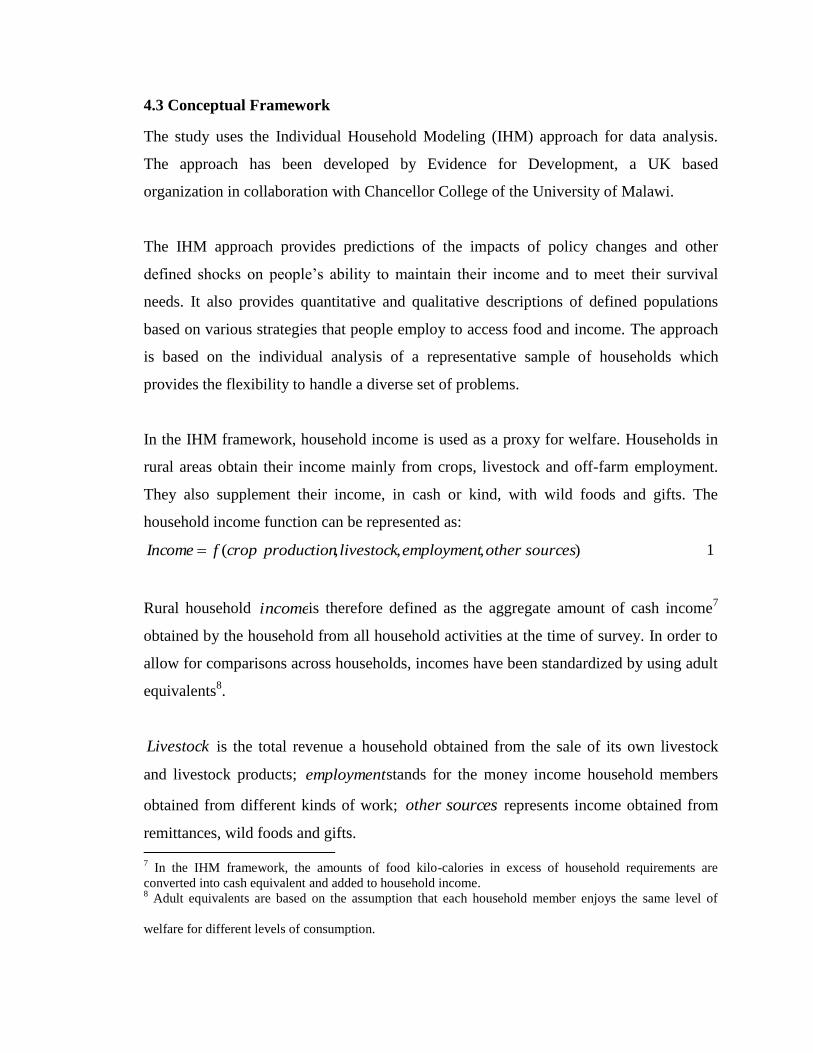
household income function can be represented as:
cropfIncome ( otheremploymentlivestockproduction ,,, )sources 1
Rural household incomeis therefore defined as the aggregate amount of cash income7
obtained by the household from all household activities at the time of survey. In order to
allow for comparisons across households, incomes have been standardized by using adult
equivalents8.
Livestock is the total revenue a household obtained from the sale of its own livestock
and livestock products; employmentstands for the money income household members
obtained from different kinds of work; other sources represents income obtained from
remittances, wild foods and gifts. 7 In the IHM framework, the amounts of food kilo-calories in excess of household requirements are
converted into cash equivalent and added to household income. 8 Adult equivalents are based on the assumption that each household member enjoys the same level of
welfare for different levels of consumption.
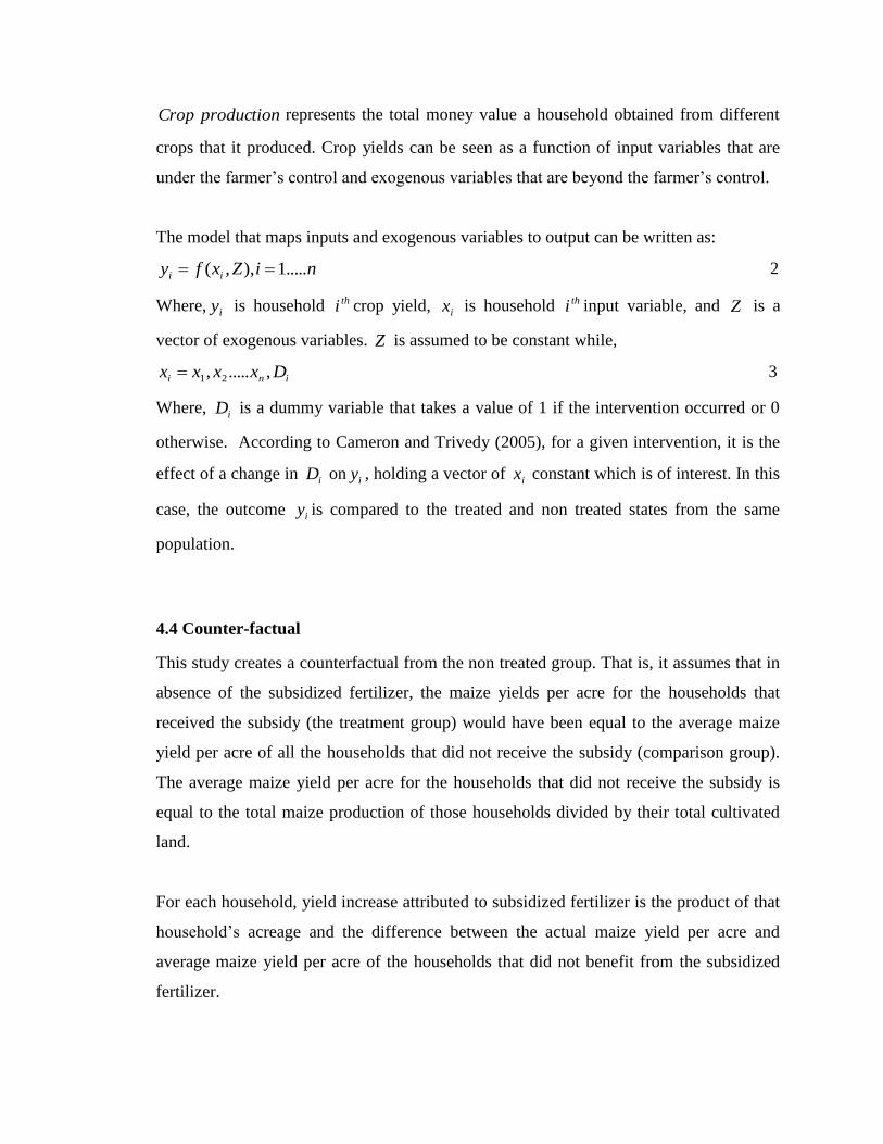
Crop production represents the total money value a household obtained from different
crops that it produced. Crop yields can be seen as a function of input variables that are
under the farmer’s control and exogenous variables that are beyond the farmer’s control.
The model that maps inputs and exogenous variables to output can be written as:
niZxfy ii .....1),,( 2
Where, iy is household thi crop yield, ix is household thi input variable, and Z is a
vector of exogenous variables. Z is assumed to be constant while,
ini Dxxxx ,....., 21 3
Where, iD is a dummy variable that takes a value of 1 if the intervention occurred or 0
otherwise. According to Cameron and Trivedy (2005), for a given intervention, it is the
effect of a change in iD on iy , holding a vector of ix constant which is of interest. In this
case, the outcome iy is compared to the treated and non treated states from the same
population.
4.4 Counter-factual
This study creates a counterfactual from the non treated group. That is, it assumes that in
absence of the subsidized fertilizer, the maize yields per acre for the households that
received the subsidy (the treatment group) would have been equal to the average maize
yield per acre of all the households that did not receive the subsidy (comparison group).
The average maize yield per acre for the households that did not receive the subsidy is
equal to the total maize production of those households divided by their total cultivated
land.
For each household, yield increase attributed to subsidized fertilizer is the product of that
household’s acreage and the difference between the actual maize yield per acre and
average maize yield per acre of the households that did not benefit from the subsidized
fertilizer.
4.5 Confounding Factors
In order to ascertain that the observed differences in maize yields are not being
influenced by factors other than application of fertilizer, the study has accounted for the
most likely confounding factor i.e. average land holding between those who used
fertilizer and those who did not. The study also accounts for income differences between
the two groups of households due to participation in other interventions.
4.6 Analytical Framework
The first step in evaluating the impact of the AISP involves establishing whether there are
statistically significant differences in yield between those who used subsidized fertilizer
and those who did not. Descriptive statistics are used to establish this. The second step
involves the use of partial budgets to calculate the net returns of subsidized fertilizer
application. A partial budget looks at only the costs and returns that have changed as a
result of fertilizer application. The calculations involved can be summarized as below:
Net iFioii OTHPFPYturns )*()*(Re,
ni .......1
4
Where, iY is household thi yield increase attributed to subsidized fertilizer; oP is the price
of output; iF is household thi quantity of fertilizer used; FP is the price of fertilizer;
iOTH are household thi costs of acquiring, applying fertilizer, and harvesting the
additional yield.9.
The third step involves conversion of households’ net returns into net returns per adult
equivalent by dividing the net returns by the appropriate households' adult equivalents.
Lastly, since the survey income values are obtained “with” the subsidy, to obtain the
“without” scenario for the households which benefited, the net returns in adult
equivalents are subtracted from the survey disposable income per adult equivalent values.
9 All beneficiaries received 1*50kg bag of fertilizer at MK850.00. Since the additional yield due to
subsidized fertilizer is not known to the farmer, the costs associated with that yield could not be quantified.
Y is in kilograms (kg) and the cost of a 50 kg bag of maize at harvesting season during which time many
farmers sell their maize to vendors was estimated at MK20/kg.
Household disposable income per adult equivalent is defined as the money income
remaining to a household after it has met its food energy requirements, divided by that
household’s adult equivalents. Calculating the household’s disposable income per adult
equivalent is a three step procedure as follows:
1. The household food energy requirement is calculated as the sum of individual
requirements of household members using United Nations (World Health
Organisation, 1985) values. Averaged over a population typical of developing country,
this approximates to 2010kcal/person/day.
2. In the case of a deficit in food production, we first establish the:
(i) The food energy which the household needs to purchase to meet its requirements;
this is equal to the calculated household food energy requirement minus the food
energy produced and consumed by the household.
(ii) then calculate the household disposable income which is equal to household money
income minus the cost of food energy to be purchased from (i).
3. The calculated disposable income for each household is then standardized by the
number of adult equivalents in the household i.e. the food requirement of the
household per an adult food requirement (average energy requirement of a young and
young female adult which is equal to 2600kcal/day.
To investigate whether the fertilizer subsidy input is associated with an increase or
decrease in food security, the study compares the proportion of households below the
food threshold “with” and “without” the subsidy. The food threshold, distinguishes
between households that are food poor and those are food sufficient. The proportions of
households falling below the thresholds represent the ultra poverty rate. The goal is to
find out whether or not the proportion of households falling below the food threshold
differ in the “with” and “without” the subsidy scenarios.
A standard of living threshold (SOLT) differentiates between households that are able to
satisfy not only their food needs but also a set of goods and services which define social
inclusion in a particular place and at a particular time. The items that constitute social
inclusion in developing countries mostly include soap, fuel, utensils and salt which are
allocated by household and, replacement clothes and, school costs which are allocated per
person and take into account age and sex. The proportion of households falling below the
SOLT represents the village poverty rate. The objective is to find out whether or not the
proportions of households below the SOLT differ in the “with” and “without” the subsidy
scenarios.
Similarly, an investigation of the targeting efficiency of the program compares the
proportion of households below and above the SOLT “without” the subsidy.
4.7 Simulation
4.7.1 Two Hundred and Fifty Percent (250%) Maize Price Increase
The study simulates the effect of an increase in the selling price of maize that comes
about due to seasonal variations. One 50kg bag of maize costs at MK1, 000. 00 during
harvesting season but the same bag costs MK2, 500.00 during traditional hunger months
of November to February, representing a 250% price increase. Suppose that households
were patient enough to wait for this price increase before selling their maize production,
how would this affect their income? The operation is executed by adjusting the price of
maize from MK20.00/kg to MK50/kg.
4.7.2 One Hundred Percent (100%) Coverage of the Village with Subsidized
Fertilizer
The study also simulates a scenario where all rural farming households benefited one
50kg bag of fertilizer. What would be the impact of 100% coverage of the village on
household poverty and food security? The simulation is based on the following
assumptions.
1. The average yield per acre without the subsidized fertilizer is 107.17kg for all
households.
2. Suppose that as a result of applying subsidized fertilizer, the seven households that
were left out from the programme achieved an average yield equal to the average yield
achieved by the twenty five households that benefited from the subsidy. That is, we
assume that fertilizer application increases the maize yield of the seven households to
322.52kg/acre.
We proceed to calculate the net returns as indicated in Appendix 2. In this case, the
“simulated 100% coverage” disposable income per adult equivalent is the sum of net
returns per adult equivalent and the without subsidy disposable income per adult
equivalent as calculated in Appendix 1.
4.8 Some Methodological Issues
Poverty measures involve three steps: choosing a quantitative welfare indicator: choosing
a means of discriminating between the poor and non poor through use of a poverty line
and finally aggregating this information into a poverty measure for a particular
population (Dercon, 2005a).
Consumption expenditure and income can alternatively be used as welfare indicators in
assessing poverty. Most studies in the developing countries prefer consumption
expenditure over income on the basis that the former tends to be smoother and more
reliable than the latter. This is said to be particularly true in rural societies where much
income is self produced in the form of agricultural goods and it is difficult to assign
income values to these enterprises (Murkherjee and Benson, 2003). In this study we use
disposable income per adult equivalent10
as a measure of welfare. This approach has an
advantage over per capita income or consumption measures since it takes into accounts
sex and age differences among household members and therefore it normalizes
consumption by taking into account household composition. Presenting the results in
terms of disposable income per adult equivalent is also a standardization method that
10
Disposable income per adult equivalent is the money income left to a household after it has met its food
needs divided by that household’s adult equivalents.
The adult equivalents are computed on the basis of energy requirements by age and sex.
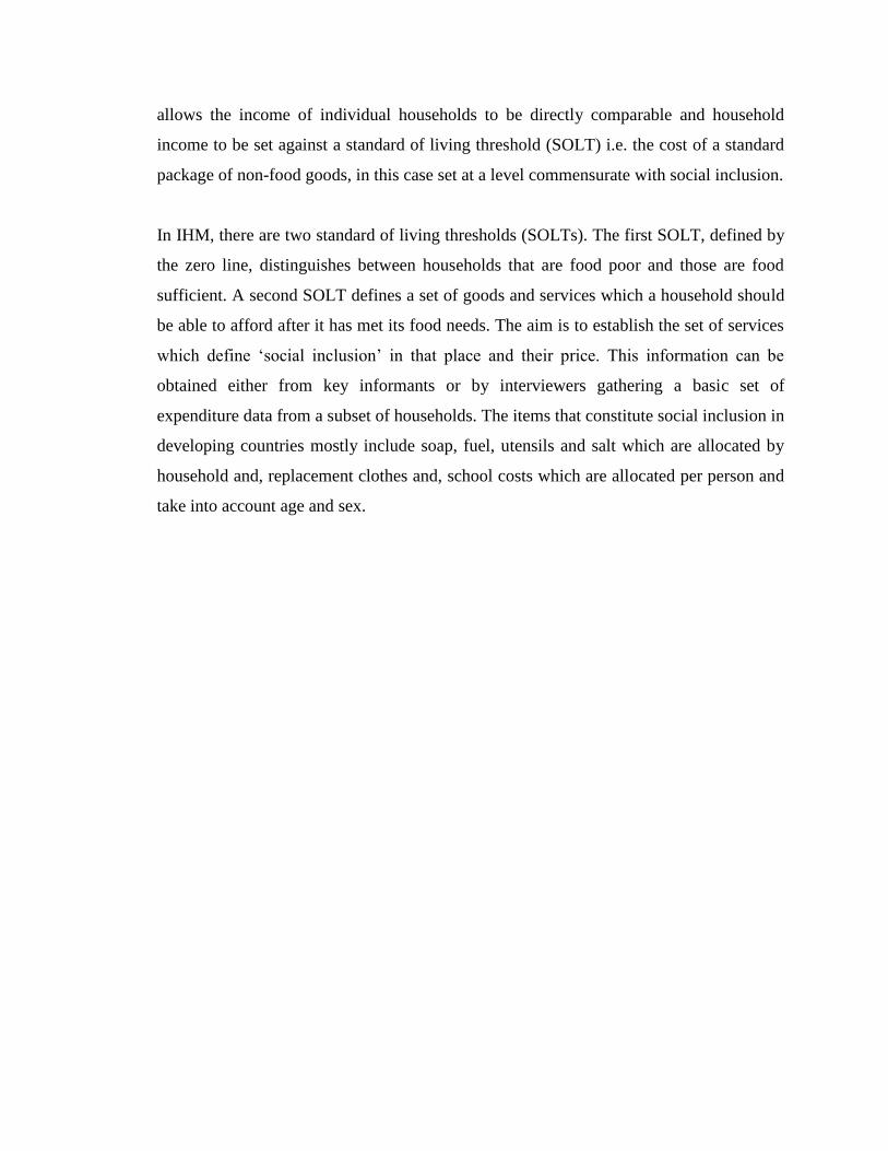
allows the income of individual households to be directly comparable and household
income to be set against a standard of living threshold (SOLT) i.e. the cost of a standard
package of non-food goods, in this case set at a level commensurate with social inclusion.
In IHM, there are two standard of living thresholds (SOLTs). The first SOLT, defined by
the zero line, distinguishes between households that are food poor and those are food
sufficient. A second SOLT defines a set of goods and services which a household should
be able to afford after it has met its food needs. The aim is to establish the set of services
which define ‘social inclusion’ in that place and their price. This information can be
obtained either from key informants or by interviewers gathering a basic set of
expenditure data from a subset of households. The items that constitute social inclusion in
developing countries mostly include soap, fuel, utensils and salt which are allocated by
household and, replacement clothes and, school costs which are allocated per person and
take into account age and sex.
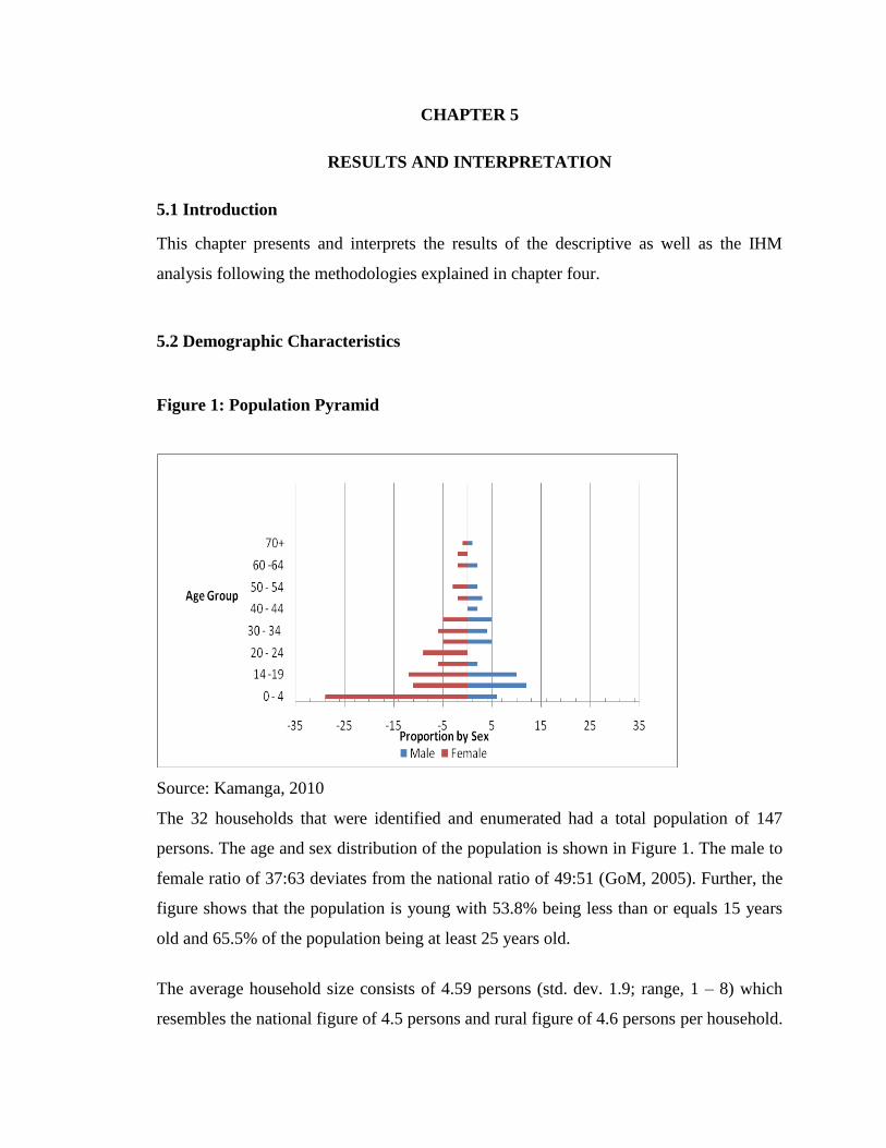
CHAPTER 5
RESULTS AND INTERPRETATION
5.1 Introduction
This chapter presents and interprets the results of the descriptive as well as the IHM
analysis following the methodologies explained in chapter four.
5.2 Demographic Characteristics
Figure 1: Population Pyramid
Source: Kamanga, 2010
The 32 households that were identified and enumerated had a total population of 147
persons. The age and sex distribution of the population is shown in Figure 1. The male to
female ratio of 37:63 deviates from the national ratio of 49:51 (GoM, 2005). Further, the
figure shows that the population is young with 53.8% being less than or equals 15 years
old and 65.5% of the population being at least 25 years old.
The average household size consists of 4.59 persons (std. dev. 1.9; range, 1 – 8) which
resembles the national figure of 4.5 persons and rural figure of 4.6 persons per household.
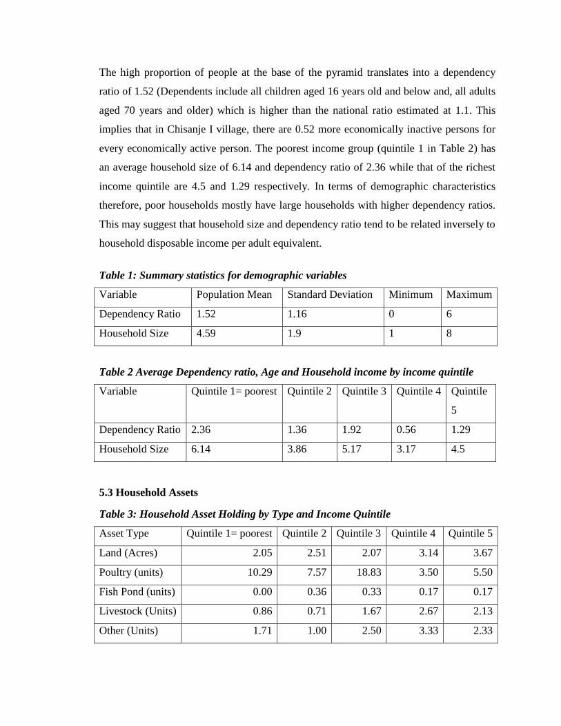
The high proportion of people at the base of the pyramid translates into a dependency
ratio of 1.52 (Dependents include all children aged 16 years old and below and, all adults
aged 70 years and older) which is higher than the national ratio estimated at 1.1. This
implies that in Chisanje I village, there are 0.52 more economically inactive persons for
every economically active person. The poorest income group (quintile 1 in Table 2) has
an average household size of 6.14 and dependency ratio of 2.36 while that of the richest
income quintile are 4.5 and 1.29 respectively. In terms of demographic characteristics
therefore, poor households mostly have large households with higher dependency ratios.
This may suggest that household size and dependency ratio tend to be related inversely to
household disposable income per adult equivalent.
Table 1: Summary statistics for demographic variables
Variable Population Mean Standard Deviation Minimum Maximum
Dependency Ratio 1.52 1.16 0 6
Household Size 4.59 1.9 1 8
Table 2 Average Dependency ratio, Age and Household income by income quintile
Variable Quintile 1= poorest Quintile 2 Quintile 3 Quintile 4 Quintile
5
Dependency Ratio 2.36 1.36 1.92 0.56 1.29
Household Size 6.14 3.86 5.17 3.17 4.5
5.3 Household Assets
Table 3: Household Asset Holding by Type and Income Quintile
Asset Type Quintile 1= poorest Quintile 2 Quintile 3 Quintile 4 Quintile 5
Land (Acres) 2.05 2.51 2.07 3.14 3.67
Poultry (units) 10.29 7.57 18.83 3.50 5.50
Fish Pond (units) 0.00 0.36 0.33 0.17 0.17
Livestock (Units) 0.86 0.71 1.67 2.67 2.13
Other (Units) 1.71 1.00 2.50 3.33 2.33
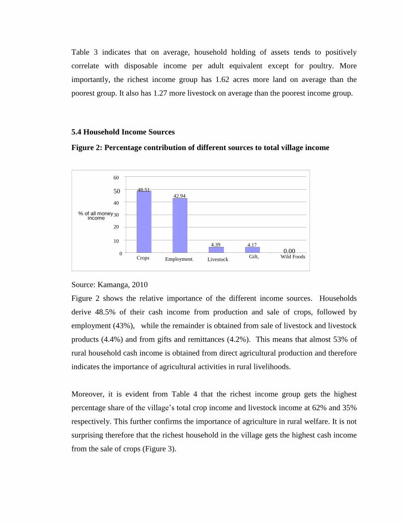
Table 3 indicates that on average, household holding of assets tends to positively
correlate with disposable income per adult equivalent except for poultry. More
importantly, the richest income group has 1.62 acres more land on average than the
poorest group. It also has 1.27 more livestock on average than the poorest income group.
5.4 Household Income Sources
Figure 2: Percentage contribution of different sources to total village income
Source: Kamanga, 2010
Figure 2 shows the relative importance of the different income sources. Households
derive 48.5% of their cash income from production and sale of crops, followed by
employment (43%), while the remainder is obtained from sale of livestock and livestock
products (4.4%) and from gifts and remittances (4.2%). This means that almost 53% of
rural household cash income is obtained from direct agricultural production and therefore
indicates the importance of agricultural activities in rural livelihoods.
Moreover, it is evident from Table 4 that the richest income group gets the highest
percentage share of the village’s total crop income and livestock income at 62% and 35%
respectively. This further confirms the importance of agriculture in rural welfare. It is not
surprising therefore that the richest household in the village gets the highest cash income
from the sale of crops (Figure 3).
48.51 42.94
4.39 4.17
0.00 0
10
20
30
40
50
60
Crops
Employment, Livestock Gift, Wild Foods
% of all money income
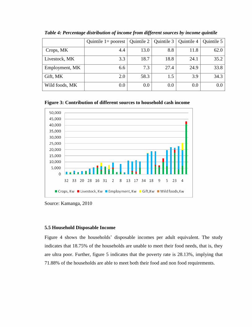
Table 4: Percentage distribution of income from different sources by income quintile
Quintile 1= poorest Quintile 2 Quintile 3 Quintile 4 Quintile 5
Crops, MK 4.4 13.0 8.8 11.8 62.0
Livestock, MK 3.3 18.7 18.8 24.1 35.2
Employment, MK 6.6 7.3 27.4 24.9 33.8
Gift, MK 2.0 58.3 1.5 3.9 34.3
Wild foods, MK 0.0 0.0 0.0 0.0 0.0
Figure 3: Contribution of different sources to household cash income
Source: Kamanga, 2010
5.5 Household Disposable Income
Figure 4 shows the households’ disposable incomes per adult equivalent. The study
indicates that 18.75% of the households are unable to meet their food needs, that is, they
are ultra poor. Further, figure 5 indicates that the poverty rate is 28.13%, implying that
71.88% of the households are able to meet both their food and non food requirements.

Figure 4: Household Disposable income per adult equivalent showing households
below the "food requirement" threshold
Source: Kamanga, 2010
Moreover, the income inequality in the village is serious. The implication is that
households in the poorest income group survive on less than the recommended
kilocalorie food energy requirement and without consumption of some basic necessities.
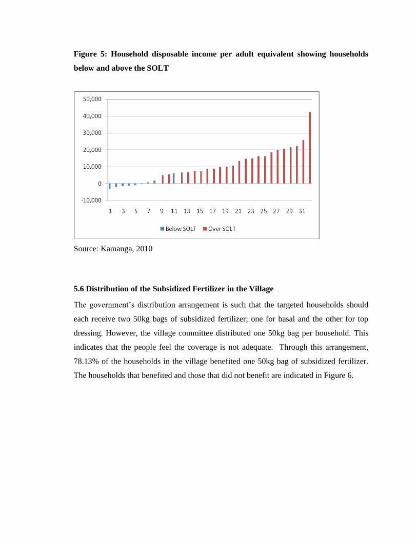
Figure 5: Household disposable income per adult equivalent showing households
below and above the SOLT
Source: Kamanga, 2010
5.6 Distribution of the Subsidized Fertilizer in the Village
The government’s distribution arrangement is such that the targeted households should
each receive two 50kg bags of subsidized fertilizer; one for basal and the other for top
dressing. However, the village committee distributed one 50kg bag per household. This
indicates that the people feel the coverage is not adequate. Through this arrangement,
78.13% of the households in the village benefited one 50kg bag of subsidized fertilizer.
The households that benefited and those that did not benefit are indicated in Figure 6.
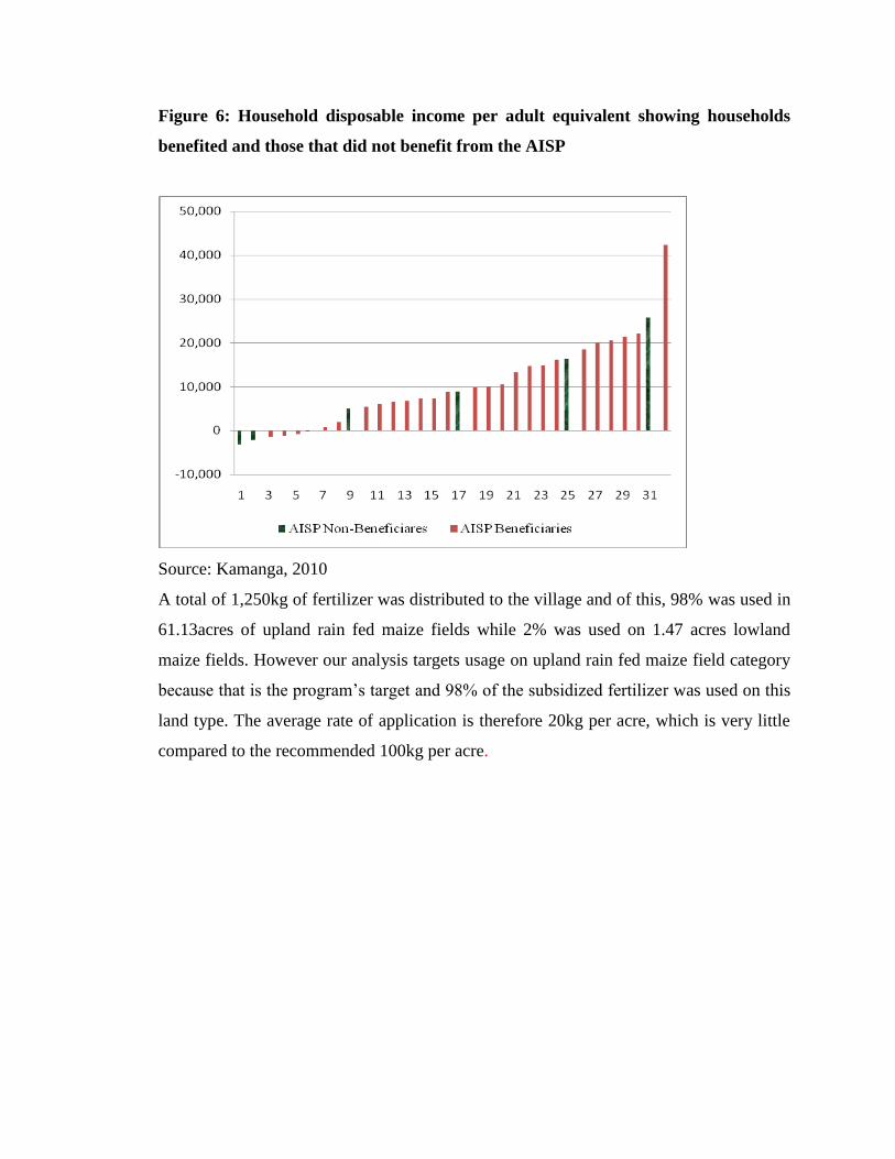
Figure 6: Household disposable income per adult equivalent showing households
benefited and those that did not benefit from the AISP
Source: Kamanga, 2010
A total of 1,250kg of fertilizer was distributed to the village and of this, 98% was used in
61.13acres of upland rain fed maize fields while 2% was used on 1.47 acres lowland
maize fields. However our analysis targets usage on upland rain fed maize field category
because that is the program’s target and 98% of the subsidized fertilizer was used on this
land type. The average rate of application is therefore 20kg per acre, which is very little
compared to the recommended 100kg per acre.
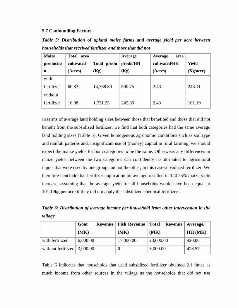
5.7 Confounding Factors
Table 5: Distribution of upland maize farms and average yield per acre between
households that received fertilizer and those that did not
Maize
productio
n
Total area
cultivated
(Acres)
Total prodn
(Kg)
Average
prodn/HH
(Kg)
Average area
cultivated/HH
(Acres)
Yield
(Kg/acre)
with
fertilizer 60.83 14,768.80 590.75 2.43 243.11
without
fertilizer 16.98 1,721.25 245.89 2.43 101.19
In terms of average land holding sizes between those that benefited and those that did not
benefit from the subsidized fertilizer, we find that both categories had the same average
land holding sizes (Table 5). Given homogenous agronomic conditions such as soil type
and rainfall patterns and, insignificant use of (money) capital in rural farming, we should
expect the maize yields for both categories to be the same. Otherwise, any differences in
maize yields between the two categories can confidently be attributed to agricultural
inputs that were used by one group and not the other, in this case subsidized fertilizer. We
therefore conclude that fertilizer application on average resulted in 140.25% maize yield
increase, assuming that the average yield for all households would have been equal to
101.19kg per acre if they did not apply the subsidized chemical fertilizers.
Table 6: Distribution of average income per household from other intervention in the
village
Goat Revenue
(MK)
Fish Revenue
(MK)
Total Revenue
(MK)
Average/
HH (MK)
with fertilizer 6,000.00 17,000.00 23,000.00 920.00
without fertilizer 3,000.00 0 3,000.00 428.57
Table 6 indicates that households that used subsidized fertilizer obtained 2.1 times as
much income from other sources in the village as the households that did not use
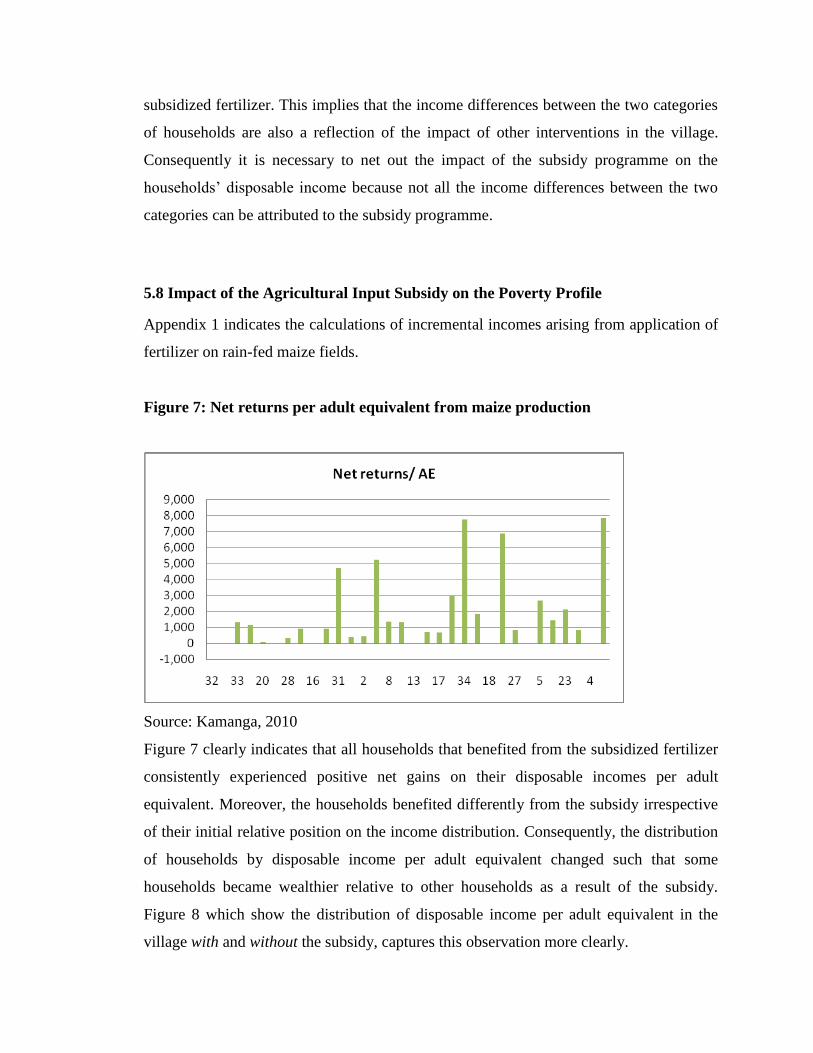
subsidized fertilizer. This implies that the income differences between the two categories
of households are also a reflection of the impact of other interventions in the village.
Consequently it is necessary to net out the impact of the subsidy programme on the
households’ disposable income because not all the income differences between the two
categories can be attributed to the subsidy programme.
5.8 Impact of the Agricultural Input Subsidy on the Poverty Profile
Appendix 1 indicates the calculations of incremental incomes arising from application of
fertilizer on rain-fed maize fields.
Figure 7: Net returns per adult equivalent from maize production
Source: Kamanga, 2010
Figure 7 clearly indicates that all households that benefited from the subsidized fertilizer
consistently experienced positive net gains on their disposable incomes per adult
equivalent. Moreover, the households benefited differently from the subsidy irrespective
of their initial relative position on the income distribution. Consequently, the distribution
of households by disposable income per adult equivalent changed such that some
households became wealthier relative to other households as a result of the subsidy.
Figure 8 which show the distribution of disposable income per adult equivalent in the
village with and without the subsidy, captures this observation more clearly.
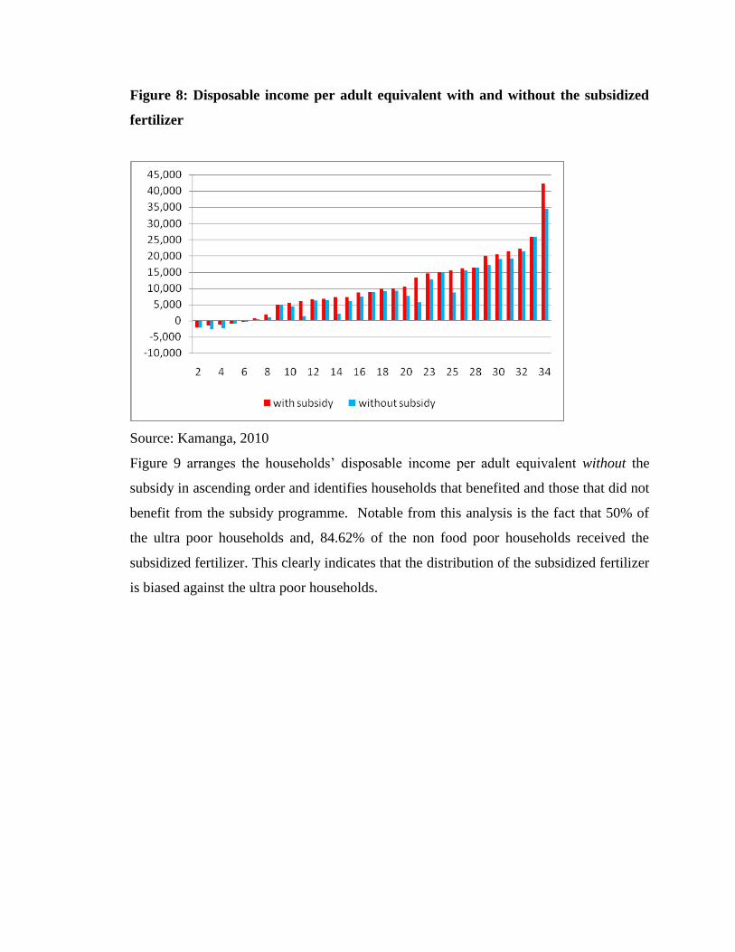
Figure 8: Disposable income per adult equivalent with and without the subsidized
fertilizer
Source: Kamanga, 2010
Figure 9 arranges the households’ disposable income per adult equivalent without the
subsidy in ascending order and identifies households that benefited and those that did not
benefit from the subsidy programme. Notable from this analysis is the fact that 50% of
the ultra poor households and, 84.62% of the non food poor households received the
subsidized fertilizer. This clearly indicates that the distribution of the subsidized fertilizer
is biased against the ultra poor households.
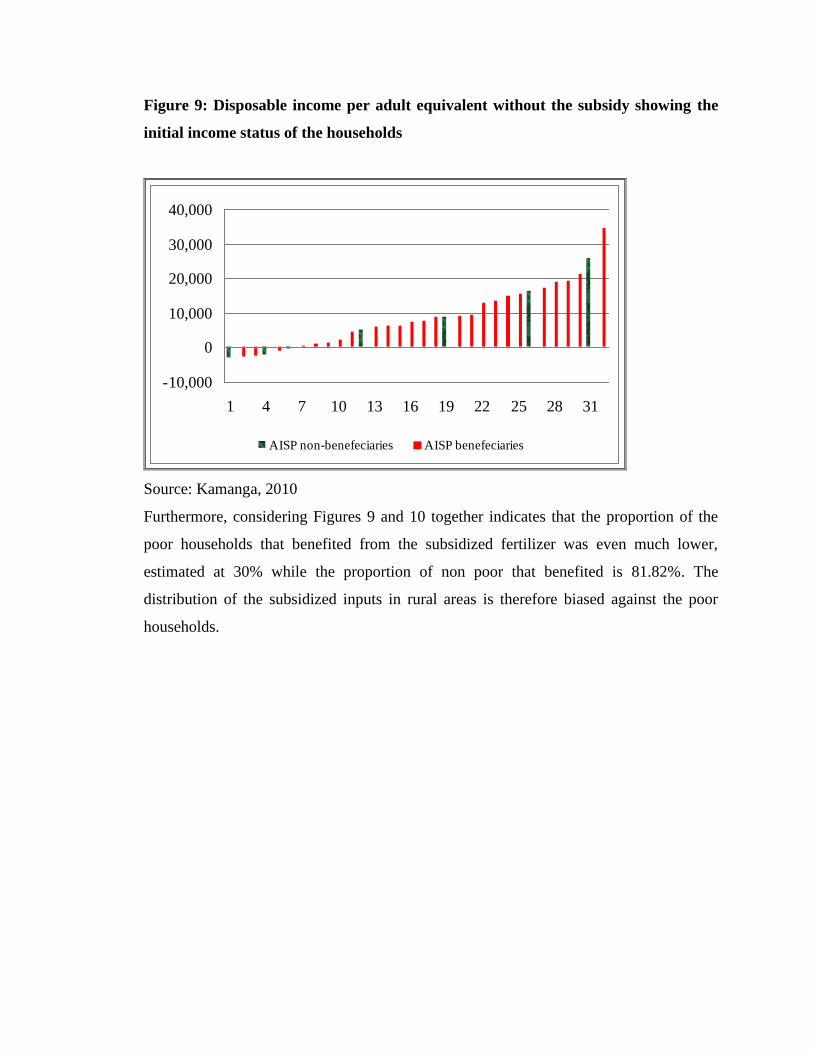
Figure 9: Disposable income per adult equivalent without the subsidy showing the
initial income status of the households
-10,000
0
10,000
20,000
30,000
40,000
1 4 7 10 13 16 19 22 25 28 31
AISP non-benefeciaries AISP benefeciaries
Source: Kamanga, 2010
Furthermore, considering Figures 9 and 10 together indicates that the proportion of the
poor households that benefited from the subsidized fertilizer was even much lower,
estimated at 30% while the proportion of non poor that benefited is 81.82%. The
distribution of the subsidized inputs in rural areas is therefore biased against the poor
households.
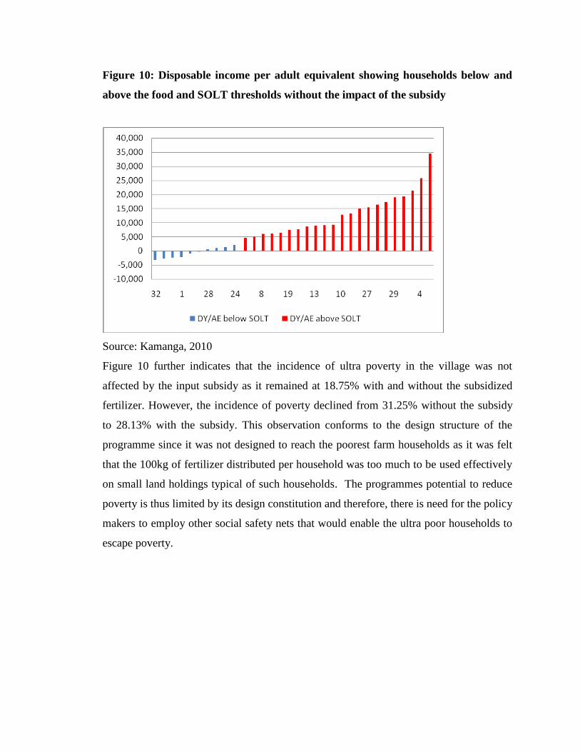
Figure 10: Disposable income per adult equivalent showing households below and
above the food and SOLT thresholds without the impact of the subsidy
Source: Kamanga, 2010
Figure 10 further indicates that the incidence of ultra poverty in the village was not
affected by the input subsidy as it remained at 18.75% with and without the subsidized
fertilizer. However, the incidence of poverty declined from 31.25% without the subsidy
to 28.13% with the subsidy. This observation conforms to the design structure of the
programme since it was not designed to reach the poorest farm households as it was felt
that the 100kg of fertilizer distributed per household was too much to be used effectively
on small land holdings typical of such households. The programmes potential to reduce
poverty is thus limited by its design constitution and therefore, there is need for the policy
makers to employ other social safety nets that would enable the ultra poor households to
escape poverty.
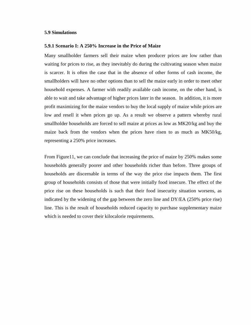
5.9 Simulations
5.9.1 Scenario I: A 250% Increase in the Price of Maize
Many smallholder farmers sell their maize when producer prices are low rather than
waiting for prices to rise, as they inevitably do during the cultivating season when maize
is scarcer. It is often the case that in the absence of other forms of cash income, the
smallholders will have no other options than to sell the maize early in order to meet other
household expenses. A farmer with readily available cash income, on the other hand, is
able to wait and take advantage of higher prices later in the season. In addition, it is more
profit maximizing for the maize vendors to buy the local supply of maize while prices are
low and resell it when prices go up. As a result we observe a pattern whereby rural
smallholder households are forced to sell maize at prices as low as MK20/kg and buy the
maize back from the vendors when the prices have risen to as much as MK50/kg,
representing a 250% price increases.
From Figure11, we can conclude that increasing the price of maize by 250% makes some
households generally poorer and other households richer than before. Three groups of
households are discernable in terms of the way the price rise impacts them. The first
group of households consists of those that were initially food insecure. The effect of the
price rise on these households is such that their food insecurity situation worsens, as
indicated by the widening of the gap between the zero line and DY/EA (250% price rise)
line. This is the result of households reduced capacity to purchase supplementary maize
which is needed to cover their kilocalorie requirements.
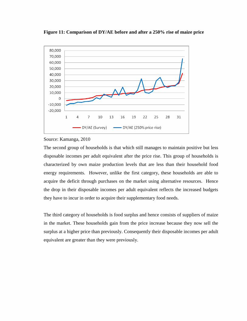
Figure 11: Comparison of DY/AE before and after a 250% rise of maize price
Source: Kamanga, 2010
The second group of households is that which still manages to maintain positive but less
disposable incomes per adult equivalent after the price rise. This group of households is
characterized by own maize production levels that are less than their household food
energy requirements. However, unlike the first category, these households are able to
acquire the deficit through purchases on the market using alternative resources. Hence
the drop in their disposable incomes per adult equivalent reflects the increased budgets
they have to incur in order to acquire their supplementary food needs.
The third category of households is food surplus and hence consists of suppliers of maize
in the market. These households gain from the price increase because they now sell the
surplus at a higher price than previously. Consequently their disposable incomes per adult
equivalent are greater than they were previously.
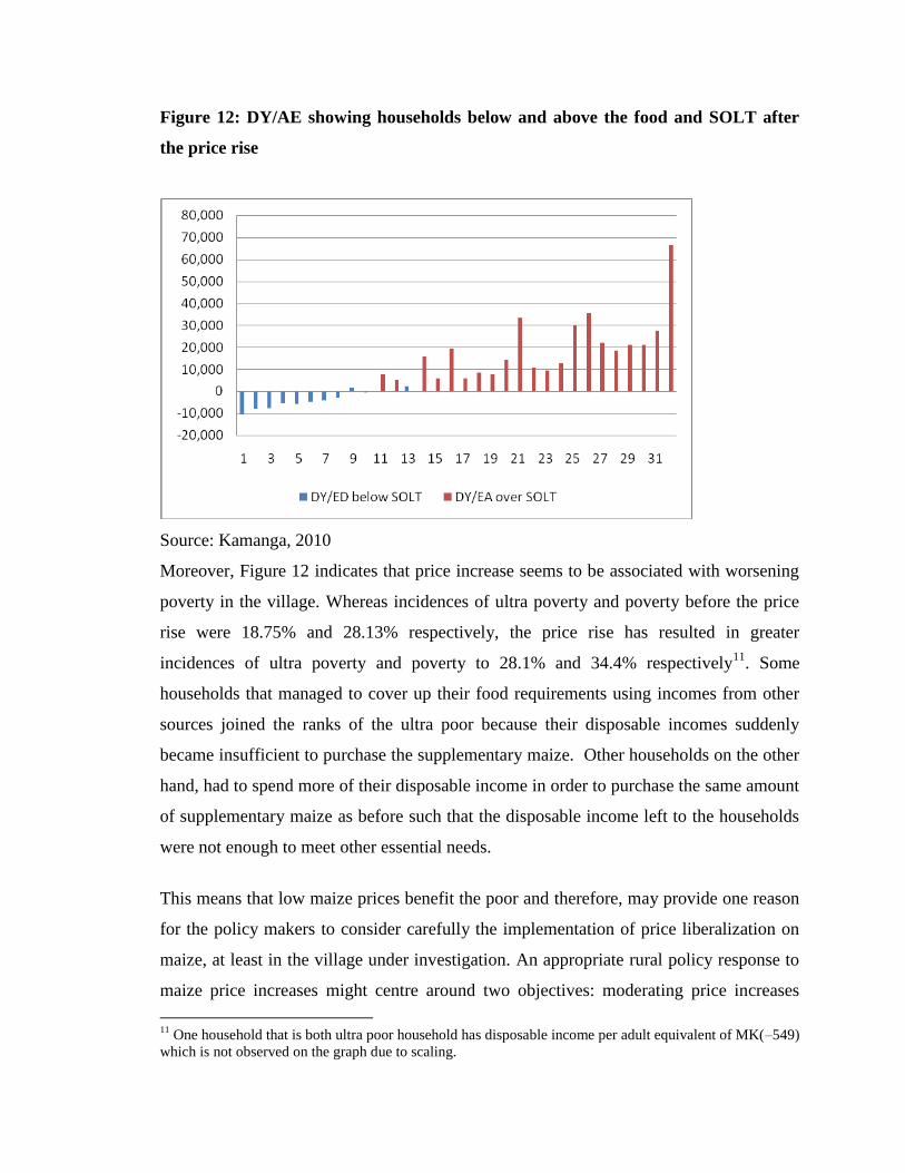
Figure 12: DY/AE showing households below and above the food and SOLT after
the price rise
Source: Kamanga, 2010
Moreover, Figure 12 indicates that price increase seems to be associated with worsening
poverty in the village. Whereas incidences of ultra poverty and poverty before the price
rise were 18.75% and 28.13% respectively, the price rise has resulted in greater
incidences of ultra poverty and poverty to 28.1% and 34.4% respectively11
. Some
households that managed to cover up their food requirements using incomes from other
sources joined the ranks of the ultra poor because their disposable incomes suddenly
became insufficient to purchase the supplementary maize. Other households on the other
hand, had to spend more of their disposable income in order to purchase the same amount
of supplementary maize as before such that the disposable income left to the households
were not enough to meet other essential needs.
This means that low maize prices benefit the poor and therefore, may provide one reason
for the policy makers to consider carefully the implementation of price liberalization on
maize, at least in the village under investigation. An appropriate rural policy response to
maize price increases might centre around two objectives: moderating price increases
11
One household that is both ultra poor household has disposable income per adult equivalent of MK(–549)
which is not observed on the graph due to scaling.
which may be achieved through price ceilings to prevent seasonal wide swings in maize
prices; and strengthening other social protection interventions through mechanisms such
as food for work and social cash transfers to avoid the most harmful coping strategies
such asset depletion.
5.8.2 Scenario II: 100% Coverage of the Village with the Input Subsidy Programme
Assuming that government does not face stringent cash constraints and that its input
subsidy program is strictly motivated by the objective of improving household food
security and income, we next consider a scenario where at least one coupon is extend all
rural farming households. The scenario is synonymous to 100% coverage of the village
such that each household receives one coupon worth one 50kg of fertilizer.
Figure 13: Comparison between survey values and 100% coverage values of DY/AE
Source: Kamanga, 2010
In figure 13 we observe that four of the households that did not previously participate in
the programme and had disposable incomes above the zero line experience improvements
in their disposable incomes per adult equivalent; two households that were unable to meet
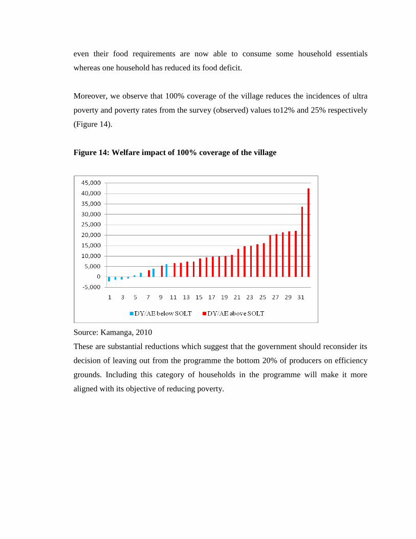
even their food requirements are now able to consume some household essentials
whereas one household has reduced its food deficit.
Moreover, we observe that 100% coverage of the village reduces the incidences of ultra
poverty and poverty rates from the survey (observed) values to12% and 25% respectively
(Figure 14).
Figure 14: Welfare impact of 100% coverage of the village
Source: Kamanga, 2010
These are substantial reductions which suggest that the government should reconsider its
decision of leaving out from the programme the bottom 20% of producers on efficiency
grounds. Including this category of households in the programme will make it more
aligned with its objective of reducing poverty.
CHAPTER 6
CONCLUSIONS AND POLICY RECOMMENDATIONS
6.1 Summary
The study set out to achieve three objectives namely, to determine whether or not AISP is
associated with poverty reduction, to find out the impact of the subsidy program on food
security, and how efficiently the programme targets the intended beneficiaries. To
achieve these objectives, a village in rural Zomba consisting of 34 households was
enumerated. The sample consisted of 25 subsidized farmers and 7 non-subsidized
farmers, while two households were declared null and void because they did not meet the
inclusion criteria. The paper employed the Individual Household Modeling (IHM)
approach to determine the three objectives.
Our empirical results indicate that the introduction of agricultural input subsidies in the
village surveyed contributes to decreasing incidence of poverty but does change the
incidence of ultra poverty. The incidence of poverty was higher (31.25%) in the village
when the income values were analyzed without the subsidy than with the subsidy
(28.13%). However, the incidence of ultra poverty remained constant at (18.75%) with
and without the subsidized fertilizer. Perhaps, for this village, direct income assistance to
the poor, in the form of fertilizer subsidies, seems to be necessary as the basis for them to
increase their incomes and improve their living conditions.
Although the study found that the intervention is overall household poverty reducing,
comparison of the proportion of poor and non poor households that benefited from the
subsidy programme indicates that the programme is biased to higher income households.
For instance, one third of the poor households benefited from the intervention compared
to over four fifth of the richer households. This clearly indicates that the intervention
achieves its objective in terms of the targeted programme beneficiaries. However, leaving
out the poorest of the poor households from the programme limits its effectiveness as an
instrument of poverty reduction. This explains why the ultra poverty rate remained
constant with and without the subsidy. In other words, the input subsidy programme does
not have an impact on food security situation of the poorer households. Food insecurity
further deepens poverty, not just in terms of negative nutritional effects on health due to
less kilocalorie intake, but also through the use of impoverishing coping mechanisms
such as asset sale which make it harder for households to lift themselves out of the
poverty trap.
Also, simulation of a 250% rise in the price of maize indicates that increasing the price of
maize is associated with worsening incidence of both ultra poverty and poverty.
Increasing the price of maize has a negative effect on the disposable income of staple-
food deficit households. This is so because such households have to spend more of their
money income on maize purchases in order to achieve households’ food requirements.
Hence the ultra poverty rate increased from 18.75% to 28.13% while the poverty rate
increased from 28.13% to 34.4%.
On the contrary, 100% coverage of the village seems to be more favourable in terms of
reducing the incidences of both ultra poverty and poverty rates in the village. This
suggests that the input subsidy programme would be more effective if it were
implemented on similar principles as the Starter Pack Programme. That is, the
programme should target all rural farming households with one 50kg bag of fertilizer
distributed to all rural farming households.
6.2 Policy Recommendations
There are several policy recommendations which can be drawn from this study, basing on
the on foregoing conclusions.
First, it is a must for policy makers to continue with policies aimed at income
redistribution and farmer support since these policies are effective in overcoming rural
poverty and achieving distributive objectives. However, these policies should be designed
to ensure the maximum effectiveness of the instruments. For example, policy makers may
consider redesigning the AISP such that the package which consists of 100kg of fertilizer
and 5kg of hybrid maize seed should be distributed to all rural farming households except
estate farmers. Such an undertaking is feasible considering that the 2005/06 AISP
covered all farming households including estate farmers. Alternatively, policy makers
should experiment with cutting down on the quantity of fertilizer by half and extending
the subsidy to more smallholder farmers especially those on the lower end of the income
distribution. As it is, the programme exacerbates rural income inequality.
Economic strategies such liberalization of the agricultural produce market should be
carefully implemented especially where demand for the produce is inelastic, as is the case
with maize in Malawi. Liberalization should be undertaken partially and with
consideration to Government’s social obligations. It seems that policy makers should
continue intervening by setting price ceilings, that is, it should be setting minimum
producer prices and maximum vendor prices in order to protect both the producer from
extremely low producer prices that makes it unprofitable to grow maize, and the
consumer from an oligopolistic maize-market structure that exists during the hunger
months. Moreover, such a policy would reduce uncertainty that arises from variations in
the input-output ratio and would therefore improve fertilizer adoption by smallholder
farmers.
Moreover, policy makers should resolve to strengthen other social protection
interventions such as the Public Works Programmes and Social Cash Transfers in order
to reach out to the poorest households which are left out from the fertilizer subsidy
programme. Otherwise the most vulnerable households will continue to engage in the
most harmful coping mechanisms such as asset depletion which exacerbate their poverty
condition. As the poverty status of households worsens, they become more marginalized
in terms of information transmission and participation in other income generating
activities. This explains why households that participated in the AISP obtained twice as
much income from other external sources as the households that did not. Consequently
such households find themselves in a vicious circle of poverty from which they may not
extricate themselves unless they are deliberately targeted with policy interventions such
as direct food and cash transfers.
6.3 Limitations
However, there are limitations to this village survey data which must be acknowledged.
First, the data collected in survey area were fixed at only one point in time. Thus, the
findings should be interpreted on the basis of the distribution of income by household
units at a point in time. Such cross sectional data fails to capture dynamic effects of
various risk factors (e.g. droughts and flooding) on production. Second, due to time and
financial constraints, data was collected at the household level only and not at the
individual level, and as such, the poverty figures obtained from this study refer to
household poverty. This makes them incomparable to national poverty figures such the
IHS.
6.4 Direction for Future Research
Future studies should be aimed at achieving a time series so that dynamics in household
welfare can tracked over time. In addition, there should be effort to capture a baseline
scenario in order to facilitate the creation of a counterfactual for each household.
REFERENCES
AFRODAD, (2002), The Politics of the MDGs and Malawi: www.afrodad.org
AFRODAD, (2005), The Politics of the MDGs and Malawi : A Critical Appraisal of the
Global Partnership for development (Goal 8): www.afrodad.org
Buffie, E. F., and M. Atolia, (2009), “Agricultural Input Subsidies in Malawi: Good, Bad,
or Hard to Tell”, FAO Commodity and Trade Policy Research Working Papers,
Trade and Markets Division, FAO.
Cameron, A. C. and P. K. Trivedi (2005), Microeconometrics: Methods and Applications,
New York: Cambridge University Press
Chilowa, W. (1998), "The Impact of Agricultural Liberalization on Food Security in
Malawi". Food Policy.
Chinsinga, B., (2002) “The Politics of Poverty Alleviation in Malawi: A Critical
Review”, Democracy of Chameleons: Politics and Vulture in New Malawi,
Englund, H., (ed.) Uppsala: Nordiska Afrika Institute.
Chinsinga, B., (2005), Practical and Policy Dilemmas of Targeting Free Inputs. In Sara
Levy (Ed.), Starter Packs: A Strategy to Fight Hunger in Developing Countries?
Wallingford, UK: CABI Publishing.
Chinsinga, B (2007), “Reclaiming policy space: lessons from Malawi’s fertilizer subsidy
Programme,” London Future Agricultures, http://www.future-agricultures.org
Chinsinga, B. and O’Brien, A. (2008). How Agricultural Subsidies are Working in
Malawi, Africa Research Institute: London.
Chirwa, E.W., (2004), Access to Land, Growth and Poverty Reduction in Malawi,
University of Malawi, Chancellor College.
Chirwa, E. W. (2007), “Sources of Technical Efficiency among Smallholder Maize
Farmers in Southern Malawi” African Economic Research Consortium
(AERC) Research Paper, No.172.
Chirwa, T.G., (2010), Program Evaluation of Agricultural Input Subsidies in Malawi
using Treatment Effects: Methods and Practicability based on Propensity Scores,
Millennium Challenge Account, Lilongwe, Malawi.
Coase, R. (1960), “The Problem of Social Cost,” Journal of Law and Economics, vol. 3,
pp. 110-18.
Crawford, E.W., T.S. Jayne, and V.A. Kelly (2005), Alternative Approaches for
Promoting Fertilizer Use in Africa, with particular Reference to the Role of
Fertilizer Subsidies, Department of Agricultural Economics, Michigan State
University, East Lansing, M148824-1039.
Crawford, E. W., T. S. Jayne and V. A. Kelly (2006), “Alternative Approaches for
Promoting fertilizer use in Africa”. Agriculture and Rural Development Discussion
Paper 22, Washington, DC, World Bank.
Cromwell, E, Kambewa, P, Mwanza, R and Chirwa, R with KWERA Development
Centre (2000), The Impact of Starter Pack on Sustainable Agriculture in Malawi,
1999-2000 Starter Pack Evaluation, Module 4, Report for Ministry of Agriculture
and Irrigation, Government of Malawi and Department of International
Development, UK.
Dercon, S. (2005), “Vulnerability: a micro perspective,” Mimeo, Oxford University.
Devereux, S., (1997) “Household Food Security in Malawi”, IDS Discussion Paper No.
362, Brighton: Institute of Development Studies.
Donovan, G., (2004) Fertilizer Subsidies in Sub-Saharan Africa: A Policy Note. Draft:
World Bank, Washington, DC
Dorward, A. (2009), “Rethinking Agricultural Input Subsidy programmes in a Changing
World,” A paper prepared for the Trade and Markets Division, FAO.
Dorward, A., E. Chirwa, V. Kelly, T.S. Jayne, R. Slater, and D. Boughton (2008),
“Evaluation of the 2006/07 Agricultural Input Subsidy Programme, Malawi.”
Final Report. Lilongwe, Malawi.
Dorward, A. and E. Chirwa, (2009), The Agricultural Input Subsidy Programme 2005 to
2008: Achievements and Challenges, London, School of Oriental and African
Studies.
Dorward, A.R., J. Kydd, J. Morrison and I. Urey (2004), “A Policy Agenda for Pro-poor
Agricultural Growth”, In A. Dorward, and J. Kydd (eds.) The Malawi 2002 Food
Crisis: The Rural Development Challenge, Journal of Modern African Studies, 42,
3 (2004), pp 343-361, Cambridge University Press.
Ellis, F. (1992), Agricultural policies in developing countries. Cambridge, Cambridge
University Press.
Frankenberger, T., and Luther, K. (2003), Review of Regional Food Security and
Nutrition Surveillance Systems in Southern Africa, CARE SWARMU.
Gore, C., (2000), The Rise and Fall of the Washington Consensus as a Paradigm for
Developing Countries, Elsevier Science Ltd, Geneva, Switzerland.
Government of Malawi, (2000), Profile of Poverty in Malawi: Poverty Analysis of the
Integrated Household Survey 1997-98,’ National Statistical Office, Zomba.
Government of Malawi, (2002), “Malawi Growth and Development Strategy: Poverty to
Prosperity 2006-2011”, Lilongwe, Ministry of Economic Planning and
Development.
Government of Malawi(2002), ‘Malawi Poverty and Reduction Strategy Paper’,
Lilongwe: Ministry of Economic Planning and Development.
Government of Malawi, (2004), “Malawi Poverty Reduction Strategy Paper”,
Lilongwe, Ministry of Economic Planning and Development.
Government of Malawi, (2005), Integrated Household Survey2, 2004-2005, Zomba:
National Statistical Office.
Government of Malawi, (2007), “Malawi Growth and Development Strategy: Poverty to
Prosperity 2006-2011”, Lilongwe, Ministry of Economic Planning and
Development.
Government of Malawi (GOM)/World Bank (2007), Malawi Poverty and Vulnerability
Assessment. Investing in Our Future. Report No. 36546-MW. Washington: World
Bank.
Gould, J.P. and C.E. Ferguson, (1980), “Microeconomic Theory,” Richard D. Irwin, Inc.
Homewood, Illinois 60430.
Gravelle, H. and R. Rees (2004), “Microeconomics,” Third Edition, Edinburgh Gate:
Pearson Education Limited.
Hardaker, B., R. Huirne, and J.R. Anderson, (1997), Coping with Risk in Agriculture,
CAB International, Wellingford.
Hanmer, L. and Nashchold (2000), “Attaining the International Development Targets:
Will Growth be Enough,” ODI Working Paper.
Harrigan, J. (1988), Malawi: The Impact of Pricing Policy on Smallholder Agriculture
19711988, Development Policy Review, 6, 415433.
Harrigan, J. (2008), “Food Insecurity, Poverty, and the Malawian Starter Pack: Fresh
Start or False Start.” Food Policy 33:237-249.
Heisey, P. W., & Mwangi, W. M. (1996). Fertilizer use and maize production in Sub-
Saharan Africa,. Mexico, D.F.: CIMMYT.
IFDC (2003) “Input Subsidies and Agricultural Development: Issues and Options for
Developing and Transitional Economies”, Discussion Paper Series 29,
International Fertilizer Development Centre: Muscle Shoals, Al
Javdani, M. (2009), “Stop the Bleeding, Heal the Wound: the Role of Fertilizer Subsidies
in Food Security, Zomba, Malawi”, An unpublished M.A. Thesis, Department of
Geography, University of Oregon.
John, S., C. Petty, P. Kambewa (2008), The Impact on Household Income and Welfare of
the pilot Social Cash Transfer and Agricultural Input Subsidy Programmes in
Mlomba TA, Machinga District, Malawi, Malawi Vulnerability Assessment
Committee, Lilongwe, Malawi.
Johnston, B,F. and J.Mellor, (1961), “The Role of Agriculture in Economic
Development,” American Economic Review 51(4), 566-593.

Kamanga, N. (2010), “The Role of Agricultural Input Subsidy Programme in Rural
Poverty Reduction: Individual Household Modeling Approach”, An unpublished
M.A. Thesis, Department of Economics, University of Malawi, Chancellor
College.
Kelly, V. (2005), “Farmers Demand for Fertilizer in Sub-Saharan Africa”, Department of
Agricultural Economics, Michigan State University.
Kherallah, M., C. Delgado, E. Gabre-Madhin, N. Minot, and M. Johnson, (2002),
Reforming Agricultural Markets in Africa, Baltimore: John Hopkins University
Press.
Kumwenda J.D.T., Waddington S.R., Snapp S.S., Jones R.B. and Blackie M.J. (1997),
Soil fertility management in the smallholder maize-based cropping systems of
Africa, in: The Emerging Maize Revolution in Africa: The Role of
Technology, Institution and Policy, East Lansing, Michigan State University.
Mann, C., (2003), Smallholder Agriculture and Productivity Growth-Starter Pack in
Malawi, Contribution to E-Discussion on Policies, Politics, Governance and
Accountability, June 9.
Mann, C. (2008). “Malawi’s Starter Pack: A Smarter Subsidy to Empower the poor with
Science- Based Agriculture”. Africa Policy Journal, John F.Kennedy School.
McCracken, K. (1983), “Planters, Peasants and the Colonial State: the Impact of the
Native Tobacco Board in the Central Province of Malawi” Journal of Southern
African Studies, 9.
Mellor, J. W., (2000), Faster More Equitable Growth: The Relation between Growth in
Agriculture and Poverty Reduction, Harvard University CAER
Mhone, G., (1987), Agriculture and Food Policy in Malawi: in T. Mkandawire (ed), The
State and Agriculture in Africa.
Minde, I., T.S. Jayne, E. Crawford, J. Ariga and J. Govereh, (2008), “Promoting
Fertilizer Use in Africa: Current Issues and Empirical Evidence from Malawi,
Zambia, and Kenya”, ReSAKSS Working Paper No. 13, CAADP, Pretoria, South
Africa.
Minot, N. (2010), Staple food prices in Malawi, Prepared for the Comesa policy
seminar on “Variation in staple food prices: Causes, consequence, and policy
options”, Maputo, Mozambique, 25-26 January 2010 under the African Agricultural
Marketing Project (AAMP).
Minot, N. and T. Benson, (2009), Fertilizer Subsidies in Africa: Are Vouchers the
Answer? International Food Policy Research Institute, Washington DC
Morris, M., V. Kelly, R. Kopicki, and D. Byerlee, (2007), Promoting Increased Fertilizer
Use in Africa: lessons Learned and Good Guidelines. Washington D.C.: World
Bank.
Mosley, P., J. Harrigan, and J. Toye (1991), “Aid and Power: The World Bank & Policy
Based Leanding,Vol. 2, Case Studies”.
Mukherjee, S., and T. Benson. 2003. “The Determinants of Poverty in Malawi, 1998.”
World Development 31 (2): 339-58.
Oygard R., Garcia, R., Guttormsen, A., Kachule, R., Mwanaumo, A., Mwanawina, I.,
Sjaastad, E. and Wik Marao,. K., Bonnerjee, A., Braithwaite, J., Carvalho, S.,
Ezemenari, K., Graham, C. and Thompson, A. (2003). The Maze of Maize:
Improving input and output market access for poor smallholders in Southern
Africa region, the experience of Zambia and Malawi. Agricultural University of
Norway, Department of Economics and Resource Management, Report no. 26.
Overseas Development Institute (ODI) (2004), Food Security Options in Malawi: Good
Neighbours make Good Friends? Country Food Security Options paper Number 2,
Forum for Food Security in Southern Africa, ODI: London.
Peltzman, S., (1976), “Toward a More General Theory of Regulation,” In G.S
Mandela and E. Miller (eds.)Microeconomic Theory and Practice, McGraw-Hill,
New York
Pender, L., Nona, E., and Rose grant, M., (2004) Soil Fertility and Fertilizer Subsidies
in sub-Saharan Africa; Issues and Recommendation, power Point presentation:
IFPRI, Washington DC.
Peters, P. (1996), Failed Magic or Social Context? Market Liberalisation and the Rural
Poor in Malawi, Harvard Institute for International Development.
Pigou, A. C. (1912). Wealth and Welfare, London: Macmillan.
Poulton, C. and A. Dorward (2008). Getting agricultural moving: role of the state in
increasing staple food crop productivity with special reference to coordination,
input subsidies, credit and price stabilization. Paper prepared for AGRA Policy
Workshop, Nairobi, Kenya, June 23–25, 2008.
Rakner, L., N. Nigeria, M. Mature and K. Schmidt, (2004), The Budget as Theatre: The
Formal and Informal International Making of the Budget Process in Malawi,
DFID: Lilongwe, Malawi.
Ravallion, M. and G. Datt, (1999), “When is Growth Pro-poor? Evidence from the
Diverse Experience of the Indian States.” World Bank Policy Research Working
Paper Series.
Ricker-Gilbert, J., T.S. Jayne and J.R. Black (2009), “Does Subsidizing Fertilizer
Increase Yields: Evidence from Malawi,” Selected paper prepared for
presentation at Agricultural and Applied Economics Association 2009 AAEA and
ACCI Joint Annual Meeting, Milwaukee, Wisconsin, July 26-29, pp. 227-240,
Michigan State University.
Rostow, W.W. (1961), The Stages of Economic Growth: A Non-Communist Manifesto,
Cambridge University Press: Cambridge.
Ruby, L., (2004), Myths that Help Perpetuate Food Insecurity in Malawi, A Power
Point Presentation, USAID Malawi.
Sahely, C., Groelsema, B., Marchione, T., and Nelson, D., (2005) The Governance
Dimensions of Food Security in Malawi, A Report Prepared for USAID Malawi:
Lilongwe, Malawi
Sahn, D., Arulpragasam, J. and Merid, L. (1990), Policy Reform and Poverty in Malawi:
A Survey of a Decade of Experience. Cornell Food and Nutrition Policy Program,
Monograph 7, December.
Sanchez, P., A. M. Isaac, R. Brush, R. Shepherd, M. Sole, U. Mokwunye, P. Woomer
and C. Ndiretu, (1997), Soil Fertility Replenishment in Africa as an Investment in
Natural Resource Capital. Madison, Soil Science Society of America.
Schultz, T. W. (1964), “Transforming Traditional Agriculture,” New Haven CT: Yale
University Press.
Sen, A. K. (1993). Capability and well-being. In M. C. Nussbaum & A. Sen (Eds.), The
Quality of life (pp. 30-53). Oxford: Clarendon Press.
Stigler, G.J. (1975), “The Citizen and the State”, In G.S Maddala and E. Miller
(eds.)Microeconomic Theory and Practice, McGraw-Hill, New York.
Stoorvogel, J.J., E.M.A. Smaling, and B.H. Janssen. (1993), Calculating soil nutrient
balances in Africa at different scales. I. Supranational scale. Fertilizer Research 35:
227-235.
Takane, T. (2007), Gambling with Liberalization: Smallholder Livelihoods in
Contemporary Rural Malawi, Institute of Development Economics, Discussion
paper No. 117
Tiffen, M. (2003), Transition in Sub Saharan Africa: Agriculture, Urbanization and
Economic Growth, World Development 31 (8), 1343-1366.
Timmer, C. P. (1997), How Well Do the Poor Connect to the Growth Response? Harvard
University, Consulting Assistance on Economic Reform II.
Tschirley, D., and T.S. Jane (2007), “Food Crisis and Food Markets: What has been
Learned in Southern Africa over the Past Decade?” FAO, Rome
Tsoka, M.G. (2006), “Poverty in Malawi and Efforts to Reduce it,” Centre for Social
Research, University of Malawi, Zomba, Malawi.
Van Donge, J, Chivwaile, M., Kapondamgaga,, Mgemezulu, O., Sangore, N. and
Thawani, E. (2001), 200102TIP: Markets and Livelihood Security in Malawi:
Lilongwe.
Weimer D. L. and A. R. Vining (2005), Policy Analysis: Concepts and Practice, Forth
Edition.
World Health Organization (1985), “Energy and Protein Requirements.” World Health
Organization technical Report No. 724, Geneva.
World Bank, 2009, “Country Assistance Strategy of the World Bank for the Republic of
Malawi.” Report No. 48336-MW (World Bank; Washington, D.C.)
Xu, Z., J. Govereh, J.R. Black and T.S. Jayne, (2006), Maize Yield Response to Fertilizer
and Profitability of Fertilizer Use among Small-scale Maize Producers in Zambia,
Contributed paper prepared for presentation at the International Association of
Agriculture Economists Conference, Gold Coast, Australia, Aug. 12-18, 2006.
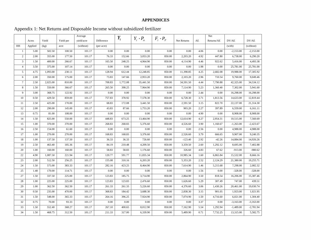
APPENDICES
Appendix 1: Net Returns and Disposable Income without subsidized fertilizer
Acres Yield Yield per
Average
yield/acre Difference iY iY * oP iF * FP
Net Returns AE
Net
Returns/AE DY/AE DY/AE
HH Applied (kg) acre (without) (per acre) (with) (without)
1 5.00 502.50 100.50 101.17 0.00 0.00 0.00 0.00 0.00 4.06 0.00 -2,153.00 -2,153.00
2 2.00 355.00 177.50 101.17 76.33 152.66 3,053.20 850.00 2,203.20 4.92 447.80 6,738.00 6,290.20
3 1.50 400.00 266.67 101.17 165.50 248.25 4,964.90 850.00 4,114.90 4.46 922.62 5,416.00 4,493.38
4 3.50 375.00 107.14 101.17 0.00 0.00 0.00 0.00 0.00 1.98 0.00 25,781.00 25,781.00
5 4.75 1,093.00 230.11 101.17 128.94 612.44 12,248.85 850.00 11,398.85 4.25 2,682.08 19,988.00 17,305.92
6 2.00 350.00 175.00 101.17 73.83 147.66 2,953.20 850.00 2,103.20 2.96 710.54 9,760.00 9,049.46
7 2.50 2,025.00 810.00 101.17 708.83 1,772.08 35,441.50 850.00 34,591.50 4.44 7,790.88 42,325.00 34,534.12
8 1.50 550.00 366.67 101.17 265.50 398.25 7,964.90 850.00 7,114.90 5.23 1,360.40 7,302.00 5,941.60
9 3.00 368.75 122.92 101.17 0.00 0.00 0.00 0.00 0.00 2.44 0.00 16,298.00 16,298.00
10 0.50 429.50 859.00 101.17 757.83 378.92 7,578.30 850.00 6,728.30 3.71 1,813.56 14,633.00 12,819.44
11 2.50 425.00 170.00 101.17 68.83 172.08 3,441.50 850.00 2,591.50 3.15 822.70 22,137.00 21,314.30
12 2.00 290.00 145.00 101.17 43.83 87.66 1,753.20 850.00 903.20 2.27 397.89 6,559.00 6,161.11
13 0.75 81.00 108.00 101.17 0.00 0.00 0.00 0.00 0.00 4.90 0.00 8,908.00 8,908.00
14 1.50 825.00 550.00 101.17 448.83 673.25 13,464.90 850.00 12,614.90 4.27 2,954.31 10,515.00 7,560.69
15 1.00 370.00 370.00 101.17 268.83 268.83 5,376.60 850.00 4,526.60 3.90 1,160.67 -1,263.00 -2,423.67
16 2.50 154.00 61.60 101.17 0.00 0.00 0.00 0.00 0.00 2.56 0.00 4,988.00 4,988.00
17 1.00 270.00 270.00 101.17 168.83 168.83 3,376.60 850.00 2,526.60 3.79 666.65 9,907.00 9,240.35
18 1.00 137.50 137.50 101.17 36.33 36.33 726.60 850.00 -123.40 2.92 -42.26 14,884.00 14,926.26
19 2.50 463.40 185.36 101.17 84.19 210.48 4,209.50 850.00 3,359.50 2.60 1,292.12 8,695.00 7,402.88
20 1.00 160.00 160.00 101.17 58.83 58.83 1,176.60 850.00 326.60 4.83 67.62 -913.00 -980.62
22 4.90 1,087.50 221.94 101.17 120.77 591.77 11,835.34 850.00 10,985.34 1.60 6,865.84 15,532.00 8,666.16
23 2.00 512.50 256.25 101.17 155.08 310.16 6,203.20 850.00 5,353.20 2.52 2,124.29 21,380.00 19,255.71
24 1.50 575.00 383.33 101.17 282.16 423.25 8,464.90 850.00 7,614.90 1.46 5,215.68 7,298.00 2,082.32
25 1.48 170.00 114.71 101.17 0.00 0.00 0.00 0.00 0.00 1.56 0.00 -328.00 -328.00
27 1.50 337.50 225.00 101.17 123.83 185.75 3,714.90 850.00 2,864.90 3.50 818.54 16,206.00 15,387.46
28 1.00 225.00 225.00 101.17 123.83 123.83 2,476.60 850.00 1,626.60 5.29 307.49 747.00 439.51
29 1.00 362.50 362.50 101.17 261.33 261.33 5,226.60 850.00 4,376.60 3.06 1,430.26 20,461.00 19,030.74
30 0.50 235.00 470.00 101.17 368.83 184.42 3,688.30 850.00 2,838.30 3.15 901.05 1,923.00 1,021.95
31 1.50 548.00 365.33 101.17 264.16 396.25 7,924.90 850.00 7,074.90 1.50 4,716.60 6,021.00 1,304.40
32 0.75 70.00 93.33 101.17 0.00 0.00 0.00 0.00 0.00 3.37 0.00 -3,163.00 -3,163.00
33 1.50 552.40 368.27 101.17 267.10 400.65 8,012.90 850.00 7,162.90 5.54 1,292.94 -1,489.00 -2,781.94
34 1.50 468.75 312.50 101.17 211.33 317.00 6,339.90 850.00 5,489.90 0.71 7,732.25 13,315.00 5,582.75
iY

Appendix 2: 100% Coverage of the Subsidy Programme
Acres Yield Yield/acre
Average
yield/acre Difference iY iY * oP
iF * FP Net Returns AE
Net returns
per
Survey
DY/AE)
Survey
DY/AE
Simulation
DY/AE
HH Applied (kg) (Kg) (without) (per acre) (with) (without)
100%
coverage
1.00 5.00 502.50 322.52 101.17 221.35 1,106.73 22,134.68 850.00 21,284.68 4.06 5,242.53 -2,153.00 -2,153.00 3,089.53
2.00 2.00 355.00 177.50 101.17 76.33 152.66 3,053.20 850.00 2,203.20 4.92 447.80 6,738.00 6,290.20 6,738.00
3.00 1.50 400.00 266.67 101.17 165.50 248.25 4,964.90 850.00 4,114.90 4.46 922.62 5,416.00 4,493.38 5,416.00
4.00 3.50 375.00 322.52 101.17 221.35 774.73 15,494.50 850.00 14,644.50 1.98 7,396.21 25,781.00 25,781.00 33,177.21
5.00 4.75 1,093.00 230.11 101.17 128.94 612.44 12,248.85 850.00 11,398.85 4.25 2,682.08 19,988.00 17,305.92 19,988.00
6.00 2.00 350.00 175.00 101.17 73.83 147.66 2,953.20 850.00 2,103.20 2.96 710.54 9,760.00 9,049.46 9,760.00
7.00 2.50 2,025.00 810.00 101.17 708.83 1,772.08 35,441.50 850.00 34,591.50 4.44 7,790.88 42,325.00 34,534.12 42,325.00
8.00 1.50 550.00 366.67 101.17 265.50 398.25 7,964.90 850.00 7,114.90 5.23 1,360.40 7,302.00 5,941.60 7,302.00
9.00 3.00 368.75 322.52 101.17 221.35 664.05 13,281.00 850.00 12,431.00 2.44 5,094.67 16,298.00 16,298.00 21,392.67
10.00 0.50 429.50 859.00 101.17 757.83 378.92 7,578.30 850.00 6,728.30 3.71 1,813.56 14,633.00 12,819.44 14,633.00
11.00 2.50 425.00 170.00 101.17 68.83 172.08 3,441.50 850.00 2,591.50 3.15 822.70 22,137.00 21,314.30 22,137.00
12.00 2.00 290.00 145.00 101.17 43.83 87.66 1,753.20 850.00 903.20 2.27 397.89 6,559.00 6,161.11 6,559.00
13.00 0.75 81.00 322.52 101.17 221.35 166.01 3,320.25 850.00 2,470.25 4.90 504.13 8,908.00 8,908.00 9,412.13
14.00 1.50 825.00 550.00 101.17 448.83 673.25 13,464.90 850.00 12,614.90 4.27 2,954.31 10,515.00 7,560.69 10,515.00
15.00 1.00 370.00 370.00 101.17 268.83 268.83 5,376.60 850.00 4,526.60 3.90 1,160.67 -1,263.00 -2,423.67 -1,263.00
16.00 2.50 154.00 322.52 101.17 221.35 553.38 11,067.50 850.00 10,217.50 2.56 3,991.21 4,988.00 4,988.00 8,979.21
17.00 1.00 270.00 270.00 101.17 168.83 168.83 3,376.60 850.00 2,526.60 3.79 666.65 9,907.00 9,240.35 9,907.00
18.00 1.00 137.50 137.50 101.17 36.33 36.33 726.60 850.00 -123.40 2.92 -42.26 14,884.00 14,926.26 14,884.00
19.00 2.50 463.40 185.36 101.17 84.19 210.48 4,209.50 850.00 3,359.50 2.60 1,292.12 8,695.00 7,402.88 8,695.00
20.00 1.00 160.00 160.00 101.17 58.83 58.83 1,176.60 850.00 326.60 4.83 67.62 -913.00 -980.62 -913.00
22.00 4.90 1,087.50 221.94 101.17 120.77 591.77 11,835.34 850.00 10,985.34 1.60 6,865.84 15,532.00 8,666.16 15,532.00
23.00 2.00 512.50 256.25 101.17 155.08 310.16 6,203.20 850.00 5,353.20 2.52 2,124.29 21,380.00 19,255.71 21,380.00
24.00 1.50 575.00 383.33 101.17 282.16 423.25 8,464.90 850.00 7,614.90 1.46 5,215.68 7,298.00 2,082.32 7,298.00
25.00 1.48 170.00 322.52 101.17 221.35 328.04 6,560.81 850.00 5,710.81 1.56 3,660.78 -328.00 -328.00 3,332.78
27.00 1.50 337.50 225.00 101.17 123.83 185.75 3,714.90 850.00 2,864.90 3.50 818.54 16,206.00 15,387.46 16,206.00
28.00 1.00 225.00 225.00 101.17 123.83 123.83 2,476.60 850.00 1,626.60 5.29 307.49 747.00 439.51 747.00
29.00 1.00 362.50 362.50 101.17 261.33 261.33 5,226.60 850.00 4,376.60 3.06 1,430.26 20,461.00 19,030.74 20,461.00
30.00 0.50 235.00 470.00 101.17 368.83 184.42 3,688.30 850.00 2,838.30 3.15 901.05 1,923.00 1,021.95 1,923.00
31.00 1.50 548.00 365.33 101.17 264.16 396.25 7,924.90 850.00 7,074.90 1.50 4,716.60 6,021.00 1,304.40 6,021.00
32.00 0.75 70.00 322.52 101.17 221.35 166.01 3,320.25 850.00 2,470.25 3.37 733.01 -3,163.00 -3,163.00 -2,429.99