Functional DifferentialGeometryGerald Jay Sussman and Jack Wisdom

AI Memo 2005-003 February 2005

© 2 0 0 5 m a s s a c h u s e t t s i n s t i t u t e o f t e c h n o l o g y, c a m b r i d g e , m a 0 2 1 3 9 u s a — w w w . c s a i l . m i t . e d u

m a ss a c h u se t t s i n st i t u t e o f t e c h n o l o g y — co m p u t e r sc i e n ce a n d a r t i f ic ia l i n t e l l ig e n ce l a b o ra t o r y

1

Abstract

Differential geometry is deceptively simple. It is surprisingly easyto get the right answer with unclear and informal symbol ma-nipulation. To address this problem we use computer programsto communicate a precise understanding of the computations indifferential geometry. Expressing the methods of differential ge-ometry in a computer language forces them to be unambiguousand computationally effective. The task of formulating a methodas a computer-executable program and debugging that programis a powerful exercise in the learning process. Also, once formal-ized procedurally, a mathematical idea becomes a tool that canbe used directly to compute results.

2

A manifold is a generalization of our idea of a smooth sur-face embedded in Euclidean space. The critical feature of ann-dimensional manifold is that locally (near any point) it lookslike n-dimensional Euclidean space: around every point there is asimply-connected open set, the coordinate patch, and a bijectivecontinuous function, the coordinate function or chart mapping ev-ery point in that open set to a tuple of n real numbers, the coordi-nates. In general, several coordinate systems are needed to labelall points on a manifold. It is required that if a region is in morethan one coordinate patch then the coordinates are consistent inthat the function mapping one set of coordinates to another iscontinuous (and perhaps differentiable to some degree). A consis-tent system of coordinate patches and coordinate functions thatcovers the entire manifold is called an atlas.1

An example of a two-dimensional manifold is the surface of asphere or of a coffee cup. The space of all configurations of a planardouble pendulum is a more abstract example of a two-dimensionalmanifold. A manifold that looks locally Euclidean may not looklike Euclidean space globally: it may not be simply connected.The surface of the coffee cup is not simply connected.

An example of a coordinate function is the function that mapspoints in a simply-connected open neighborhood of a sphere to thetuple of latitude and longitude.2 If we want to talk about motionon the Earth, we can identify the space of configurations to a2-sphere. The map from the 2-sphere to the three-dimensionalcoordinates of a point on the surface of the Earth captures theshape of the Earth.

Two angles specify the configuration of the planar double pen-dulum. The manifold of configurations is a torus, and each anglerequires two coordinate patches to cover it (because angles wraparound). Each point on the torus corresponds to a configuration ofthe double pendulum, specifying the position of each constituentin space. The constraints, such as the lengths of the pendulum

1We may impose a non-Euclidean metric on the coordinates. For example,the coordinates used in relativity have a metric structure that does not obeythe requirement that distinct points have non-zero distance between them.

2The open set for a latitude-longitude coordinate system may not includeeither pole (because longitude is not defined at the poles) or on the 180◦

meridian (where the longitude is discontinuous). Other coordinate systemsare needed for these places.

3

χ

χf

f

f(m)

Mm

Rn

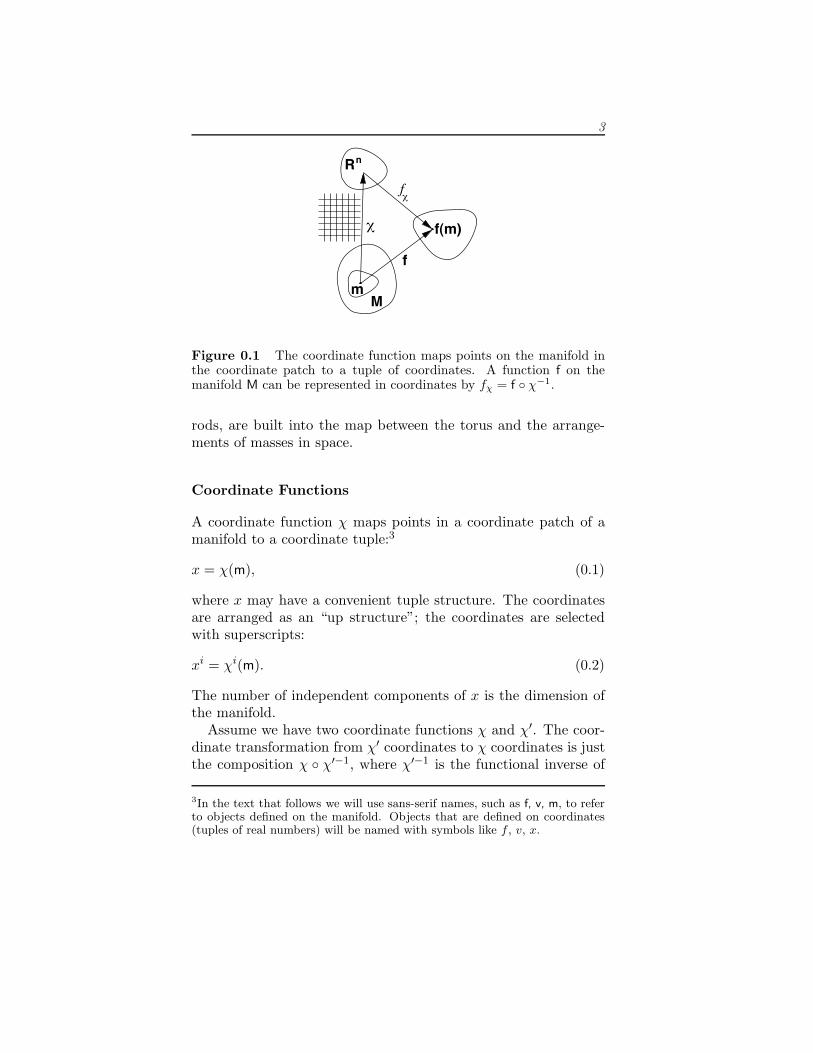
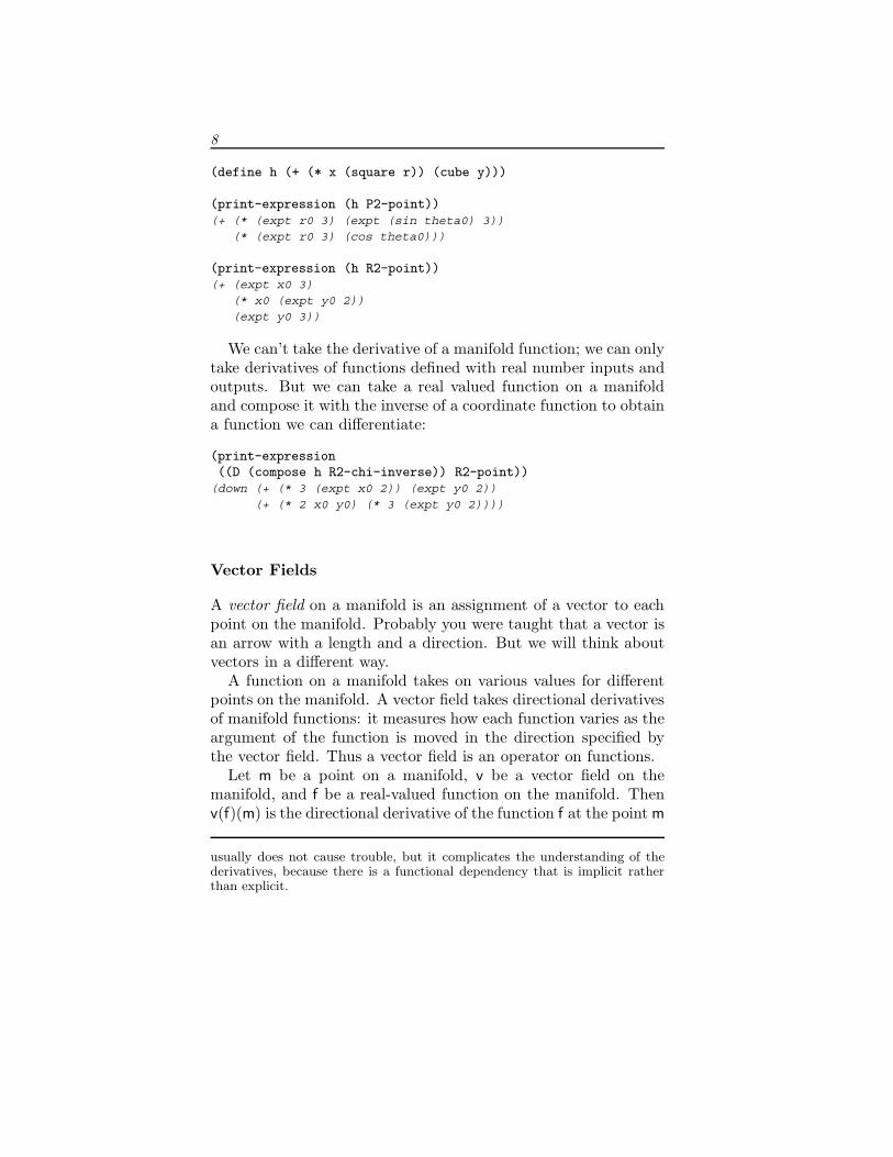
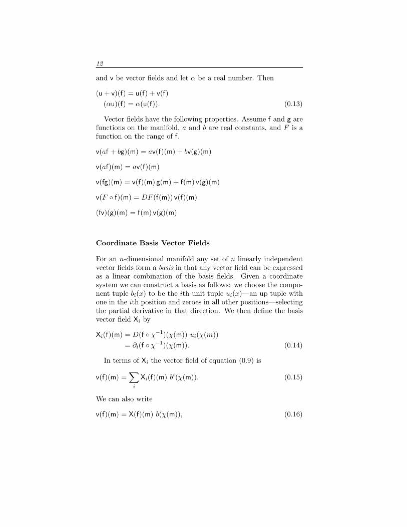
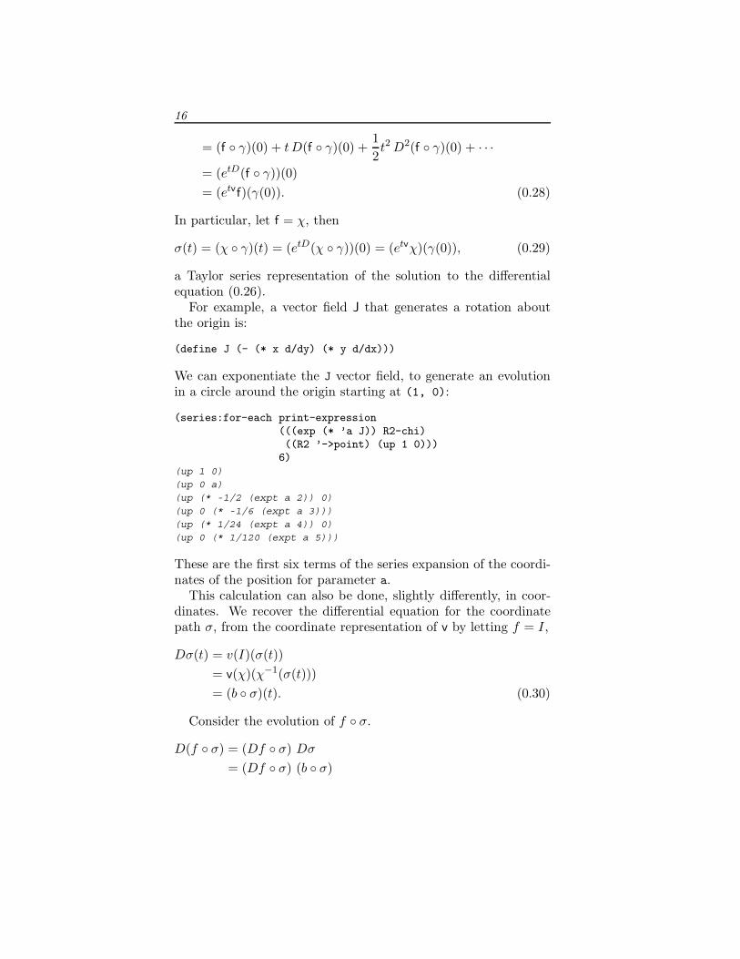
Figure 0.1 The coordinate function maps points on the manifold inthe coordinate patch to a tuple of coordinates. A function f on themanifold M can be represented in coordinates by fχ = f ◦ χ−1.

rods, are built into the map between the torus and the arrange-ments of masses in space.

Coordinate Functions

A coordinate function χ maps points in a coordinate patch of amanifold to a coordinate tuple:3

x = χ(m), (0.1)

where x may have a convenient tuple structure. The coordinatesare arranged as an “up structure”; the coordinates are selectedwith superscripts:

xi = χi(m). (0.2)

The number of independent components of x is the dimension ofthe manifold.

Assume we have two coordinate functions χ and χ′. The coor-dinate transformation from χ′ coordinates to χ coordinates is justthe composition χ ◦ χ′−1, where χ′−1 is the functional inverse of

3In the text that follows we will use sans-serif names, such as f, v, m, to referto objects defined on the manifold. Objects that are defined on coordinates(tuples of real numbers) will be named with symbols like f , v, x.

4

χ’

χ’χ−1

oRn

Rn

χ

Mm

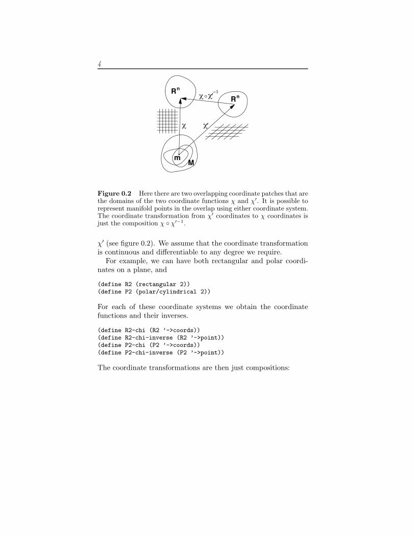
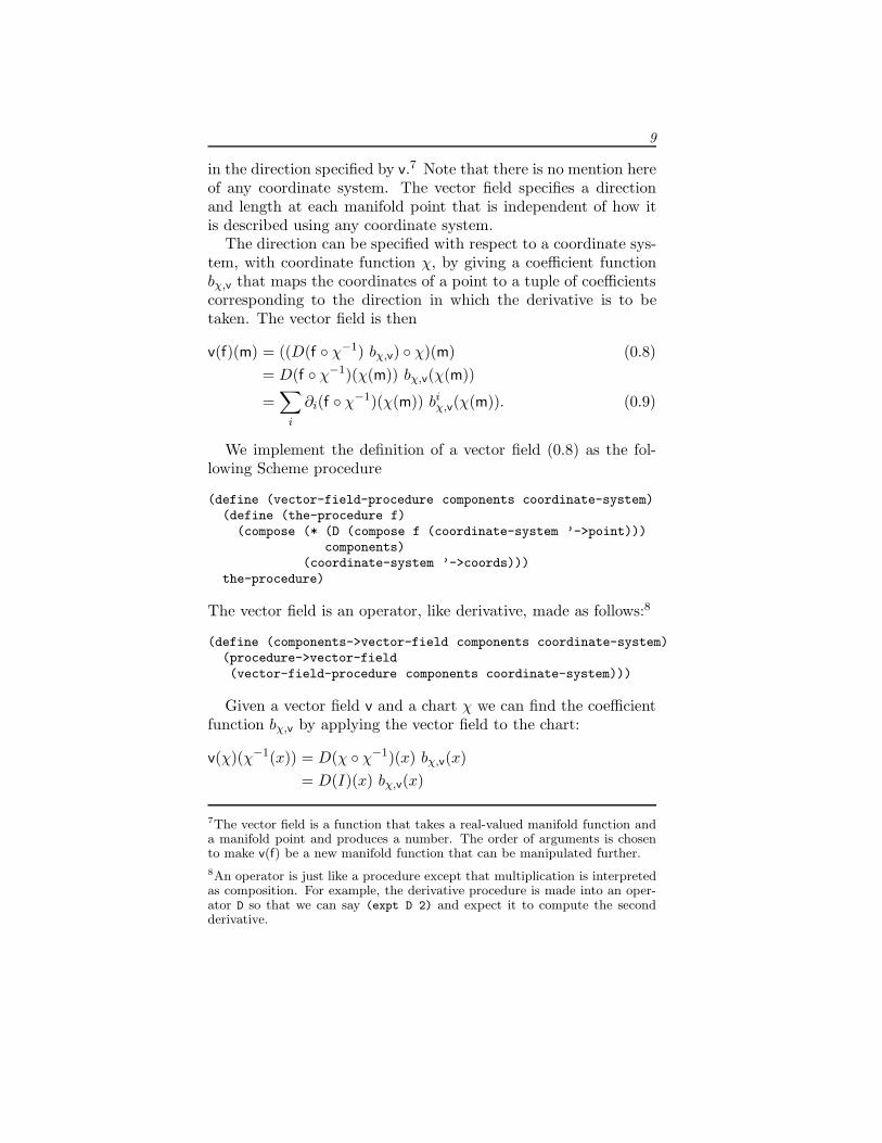
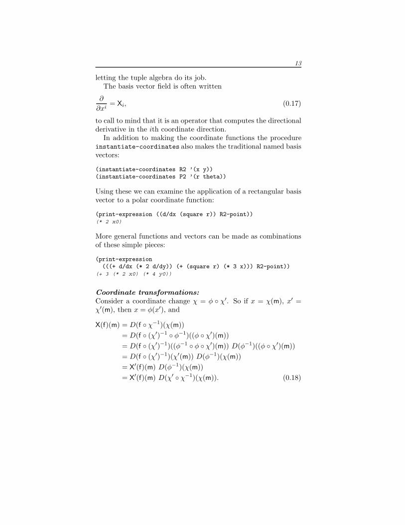
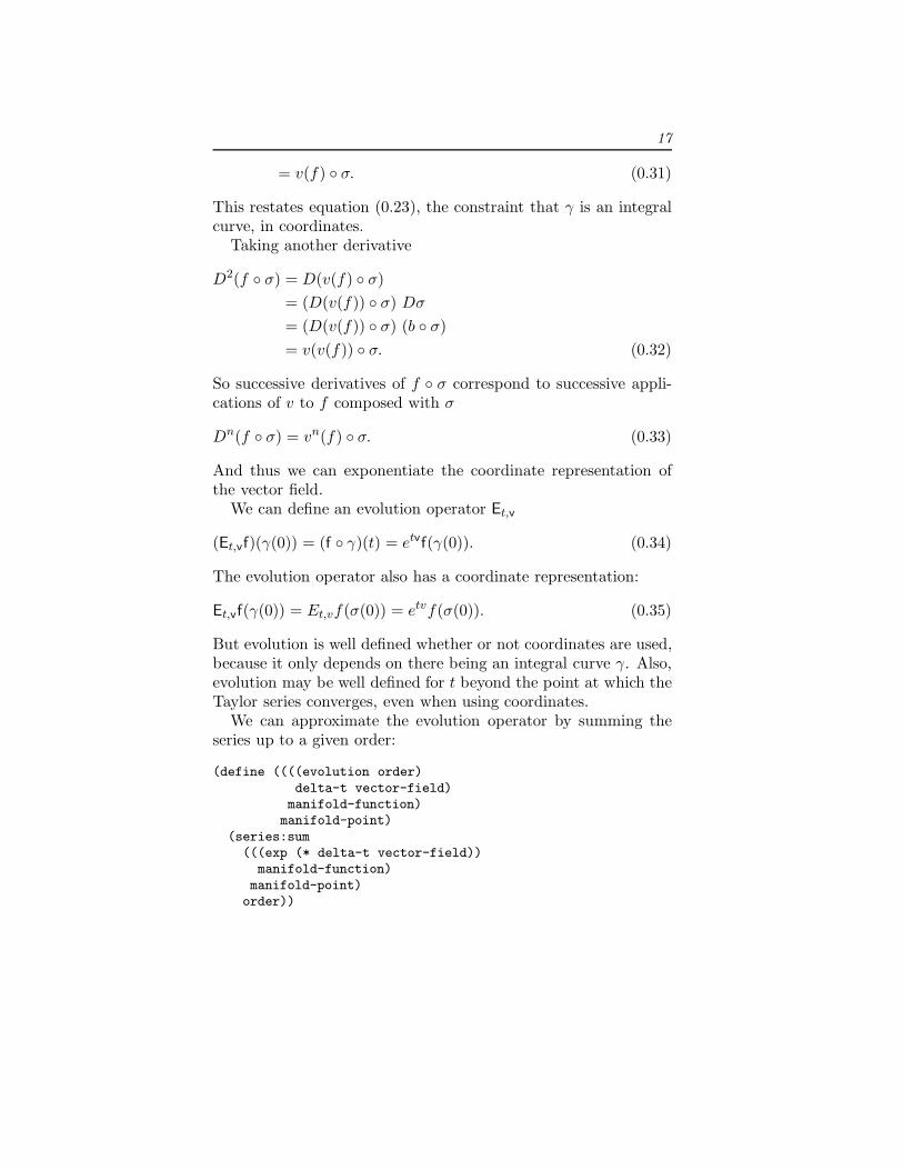
Figure 0.2 Here there are two overlapping coordinate patches that arethe domains of the two coordinate functions χ and χ′. It is possible torepresent manifold points in the overlap using either coordinate system.The coordinate transformation from χ′ coordinates to χ coordinates isjust the composition χ ◦ χ′−1.

χ′ (see figure 0.2). We assume that the coordinate transformationis continuous and differentiable to any degree we require.

For example, we can have both rectangular and polar coordi-nates on a plane, and

(define R2 (rectangular 2))(define P2 (polar/cylindrical 2))

For each of these coordinate systems we obtain the coordinatefunctions and their inverses.

(define R2-chi (R2 ’->coords))(define R2-chi-inverse (R2 ’->point))(define P2-chi (P2 ’->coords))(define P2-chi-inverse (P2 ’->point))

The coordinate transformations are then just compositions:

5

(print-expression((compose P2-chi R2-chi-inverse)(up ’x0 ’y0)))

(up (sqrt (+ (expt x0 2) (expt y0 2))) (atan y0 x0))

(print-expression((compose R2-chi P2-chi-inverse)(up ’r0 ’theta0)))

(up (* r0 (cos theta0)) (* r0 (sin theta0)))

And we can obtain the Jacobian of the transformation by takingits derivative4

(print-expression((D (compose R2-chi P2-chi-inverse))(up ’r0 ’theta0)))

(down (up (cos theta0) (sin theta0))(up (* -1 r0 (sin theta0)) (* r0 (cos theta0))))

Manifold Functions:Let f be a function on a manifold M. This function has a coor-dinate representation fχ with respect to the coordinate functionχ:

fχ = f ◦ χ−1. (0.3)

The value of fχ(x) is independent of coordinates:

fχ(x) = (f ◦ χ−1)(χ(m)) = f(m). (0.4)

The subscript χ may be dropped when it is unambiguous.The manifold point m is represented in rectangular coordinates

by a pair of real numbers,

(x, y) = χ(m), (0.5)

and the manifold function f is represented in rectangular coordi-nates by f that takes a pair of real numbers and produces a realnumber

f : R2 → R

4See SICM, Appendix 8, for an introduction to tuple arithmetic and a discus-sion of derivatives of functions with structured input or output.

6

f : (x, y) �→ f(x, y). (0.6)

We define our manifold function

f : M → R

f : m �→ (f ◦ χ)(m). (0.7)

We can illustrate the coordinate independence with a program.We will show that an arbitrary manifold function f, when definedby its coordinate representation in rectangular coordinates, hasthe same behavior when applied to a manifold point independentof whether the point is specified in rectangular or polar coordi-nates.

First define a signature for functions that map an up structureof two reals to a real, then define a manifold function by specifyingits behavior in rectangular coordinates:5

(define R2->R (-> (UP Real Real) Real))

(define f(compose (literal-function ’f-rect R2->R)

R2-chi))

A typical point can be specified using each coordinate system:

(define R2-point (R2-chi-inverse (up ’x0 ’y0)))(define P2-point (P2-chi-inverse (up ’r0 ’theta0)))

The definition of the function f is independent of the coordinatesystem used to specify the point of evaluation:

(print-expression (f R2-point))(f-rect (up x0 y0))

(print-expression (f P2-point))(f-rect (up (* r0 (cos theta0)) (* r0 (sin theta0))))

5Alternatively, we can define the same function in a shorthand

(define f (literal-manifold-function ’f-rect R2))

7

And, similarly, a function defined in terms of its behavior in po-lar coordinates makes sense when applied to a point specified inrectangular coordinates.

(define g (literal-manifold-function ’g-polar P2))

(print-expression (g P2-point))(g-polar (up r0 theta0))

(print-expression (g R2-point))(g-polar

(up (sqrt (+ (expt x0 2) (expt y0 2)))(atan y0 x0)))

To make things a bit easier, we can give names to the individualcoordinate functions associated with a coordinate system. Herewe name the coordinate functions for the R2 coordinate system xand y and for the P2 coordinate system r and theta.

(instantiate-coordinates R2 ’(x y))(instantiate-coordinates P2 ’(r theta))

This allows us to extract the coordinates from a point, indepen-dent of the coordinate system used to specify the point.

(print-expression (x R2-point))x0

(print-expression (x P2-point))(* r0 (cos theta0))

(print-expression (r P2-point))r0

(print-expression (r R2-point))(sqrt (+ (expt x0 2) (expt y0 2)))

(print-expression (theta R2-point))(atan y0 x0)

We can work with the coordinate functions in a natural manner,defining new manifold functions in terms of them:6

6This is actually a nasty, but traditional, abuse of notation. The problem isthat cos r really means cos ◦r, or in Scheme notation (square r) really means(compose square r). Both have been made to work in our system. This

8

(define h (+ (* x (square r)) (cube y)))

(print-expression (h P2-point))(+ (* (expt r0 3) (expt (sin theta0) 3))

(* (expt r0 3) (cos theta0)))

(print-expression (h R2-point))(+ (expt x0 3)

(* x0 (expt y0 2))(expt y0 3))

We can’t take the derivative of a manifold function; we can onlytake derivatives of functions defined with real number inputs andoutputs. But we can take a real valued function on a manifoldand compose it with the inverse of a coordinate function to obtaina function we can differentiate:

(print-expression((D (compose h R2-chi-inverse)) R2-point))

(down (+ (* 3 (expt x0 2)) (expt y0 2))(+ (* 2 x0 y0) (* 3 (expt y0 2))))

Vector Fields

A vector field on a manifold is an assignment of a vector to eachpoint on the manifold. Probably you were taught that a vector isan arrow with a length and a direction. But we will think aboutvectors in a different way.

A function on a manifold takes on various values for differentpoints on the manifold. A vector field takes directional derivativesof manifold functions: it measures how each function varies as theargument of the function is moved in the direction specified bythe vector field. Thus a vector field is an operator on functions.

Let m be a point on a manifold, v be a vector field on themanifold, and f be a real-valued function on the manifold. Thenv(f)(m) is the directional derivative of the function f at the point m

usually does not cause trouble, but it complicates the understanding of thederivatives, because there is a functional dependency that is implicit ratherthan explicit.

9

in the direction specified by v.7 Note that there is no mention hereof any coordinate system. The vector field specifies a directionand length at each manifold point that is independent of how itis described using any coordinate system.

The direction can be specified with respect to a coordinate sys-tem, with coordinate function χ, by giving a coefficient functionbχ,v that maps the coordinates of a point to a tuple of coefficientscorresponding to the direction in which the derivative is to betaken. The vector field is then

v(f)(m) = ((D(f ◦ χ−1) bχ,v) ◦ χ)(m) (0.8)= D(f ◦ χ−1)(χ(m)) bχ,v(χ(m))

=∑

i

∂i(f ◦ χ−1)(χ(m)) biχ,v(χ(m)). (0.9)

We implement the definition of a vector field (0.8) as the fol-lowing Scheme procedure

(define (vector-field-procedure components coordinate-system)(define (the-procedure f)(compose (* (D (compose f (coordinate-system ’->point)))

components)(coordinate-system ’->coords)))

the-procedure)

The vector field is an operator, like derivative, made as follows:8

(define (components->vector-field components coordinate-system)(procedure->vector-field(vector-field-procedure components coordinate-system)))

Given a vector field v and a chart χ we can find the coefficientfunction bχ,v by applying the vector field to the chart:

v(χ)(χ−1(x)) = D(χ ◦ χ−1)(x) bχ,v(x)= D(I)(x) bχ,v(x)

7The vector field is a function that takes a real-valued manifold function anda manifold point and produces a number. The order of arguments is chosento make v(f) be a new manifold function that can be manipulated further.

8An operator is just like a procedure except that multiplication is interpretedas composition. For example, the derivative procedure is made into an oper-ator D so that we can say (expt D 2) and expect it to compute the secondderivative.

10

= bχ,v(x) (0.10)

So we can use a vector field v to measure the rate of change ofthe coordinates χ in the direction specified by v at each point mon the manifold. The result is a function bχ,v of the coordinatesof the point in the manifold. Each component of bχ,v specifies therate of change of a coordinate in the direction and rate specifiedby v.

Because the coordinates are an up structure, the derivativemakes a down structure, and the coefficient tuple bχ,v(x) is an upstructure compatible for addition to the coordinates. Note thatfor any vector field v the coefficients bχ,v(x) are different for differ-ent coordinate functions χ. In the text that follows we will usuallydrop the subscripts on b, understanding that it is dependent onthe coordinate system and the vector field.

Given a coordinate system and coefficient functions that mapcoordinates to real values, we can make a vector field. For exam-ple, a general vector field can be defined by giving componentsrelative to the coordinate system R2 by9

(define v(components->vector-field(up (literal-function ’vx (-> (UP Real Real) Real))

(literal-function ’vy (-> (UP Real Real) Real)))R2))

When this vector field is applied to an arbitrary manifold functionwe see that it gives the directional derivative of that manifoldfunction in the direction specified by the components vx and vy.

(print-expression((v (literal-manifold-function ’f R2)) R2-point))

(+ (* (((partial 0) f) (up x0 y0)) (vx (up x0 y0)))(* (((partial 1) f) (up x0 y0)) (vy (up x0 y0))))

9To make it convenient to define literal vector fields we provide a shorthand:

(define w (literal-vector-field ’v R2))

This makes a vector field with component functions named vˆ0 and vˆ1 andnames the result w.

11

The vector field v has a coordinate representation v:

v(f)(m) = D(f ◦ χ−1)(χ(m)) b(χ(m))= Df(x) b(x)= v(f)(x), (0.11)

with the definitions f = f ◦ χ−1 and x = χ(m). The function b isthe coefficient function for the vector field v. It provides a scalefactor for the component in each coordinate direction. However, vis the coordinate representation of the vector field f in that it takesdirectional derivatives of coordinate representations of manifoldfunctions.

Given a vector field v and a coordinate system coordsys we canconstruct the coordinate representation of the vector field.10

(define (coordinatize vector-field coordsys)(define ((v f) x)(let ((b (compose (vector-field (coordsys ’->coords))

(coordsys ’->point))))(* ((D f) x) (b x)))))

(make-operator v))

We can apply a coordinatized vector field to a function of coordi-nates to get the same answer as before.

(print-expression(((coordinatize v R2)

(literal-function ’f (-> (UP Real Real) Real)))(up ’x0 ’y0)))

(+ (* (((partial 0) f) (up x0 y0)) (vx (up x0 y0)))(* (((partial 1) f) (up x0 y0)) (vy (up x0 y0))))

For the manifold Rn we can let χ = I. Then x = m, f = f, and

v(f)(x) = Df(x) b(x), (0.12)

which is the usual directional derivative.

Vector Field Properties:The vector fields on a manifold form a vector space over the reals,with the sum and scalar multiplication defined as follows. Let u

10The make-operator procedure takes a procedure and returns an operator.

12

and v be vector fields and let α be a real number. Then

(u + v)(f) = u(f) + v(f)(αu)(f) = α(u(f)). (0.13)

Vector fields have the following properties. Assume f and g arefunctions on the manifold, a and b are real constants, and F is afunction on the range of f.

v(af + bg)(m) = av(f)(m) + bv(g)(m)

v(af)(m) = av(f)(m)

v(fg)(m) = v(f)(m) g(m) + f(m) v(g)(m)

v(F ◦ f)(m) = DF (f(m)) v(f)(m)

(fv)(g)(m) = f(m) v(g)(m)

Coordinate Basis Vector Fields

For an n-dimensional manifold any set of n linearly independentvector fields form a basis in that any vector field can be expressedas a linear combination of the basis fields. Given a coordinatesystem we can construct a basis as follows: we choose the compo-nent tuple bi(x) to be the ith unit tuple ui(x)—an up tuple withone in the ith position and zeroes in all other positions—selectingthe partial derivative in that direction. We then define the basisvector field Xi by

Xi(f)(m) = D(f ◦ χ−1)(χ(m)) ui(χ(m))= ∂i(f ◦ χ−1)(χ(m)). (0.14)

In terms of Xi the vector field of equation (0.9) is

v(f)(m) =∑

i

Xi(f)(m) bi(χ(m)). (0.15)

We can also write

v(f)(m) = X(f)(m) b(χ(m)), (0.16)

13

letting the tuple algebra do its job.The basis vector field is often written

∂

∂xi= Xi, (0.17)

to call to mind that it is an operator that computes the directionalderivative in the ith coordinate direction.

In addition to making the coordinate functions the procedureinstantiate-coordinates also makes the traditional named basisvectors:

(instantiate-coordinates R2 ’(x y))(instantiate-coordinates P2 ’(r theta))

Using these we can examine the application of a rectangular basisvector to a polar coordinate function:

(print-expression ((d/dx (square r)) R2-point))(* 2 x0)

More general functions and vectors can be made as combinationsof these simple pieces:

(print-expression(((+ d/dx (* 2 d/dy)) (+ (square r) (* 3 x))) R2-point))

(+ 3 (* 2 x0) (* 4 y0))

Coordinate transformations:Consider a coordinate change χ = φ ◦ χ′. So if x = χ(m), x′ =χ′(m), then x = φ(x′), and

X(f)(m) = D(f ◦ χ−1)(χ(m))= D(f ◦ (χ′)−1 ◦ φ−1)((φ ◦ χ′)(m))= D(f ◦ (χ′)−1)((φ−1 ◦ φ ◦ χ′)(m)) D(φ−1)((φ ◦ χ′)(m))= D(f ◦ (χ′)−1)(χ′(m)) D(φ−1)(χ(m))= X′(f)(m) D(φ−1)(χ(m))= X′(f)(m) D(χ′ ◦ χ−1)(χ(m)). (0.18)

14

This is the rule for the transformation of basis vector fields. Thesecond factor can be recognized as “∂x′/∂x”.11

The vector field does not depend on coordinates. So, fromequation (0.16), we have

v(f)(m) = X(f)(m) b(χ(m))= X′(f)(m) b′(χ′(m)) (0.19)

Using equation (0.18), we deduce

D(φ−1)(x) b(x) = b′(x′). (0.20)

Because φ−1 ◦ φ = I, we have

D(φ−1)(x) = (Dφ(x′))−1, (0.21)

and so

b(x) = Dφ(x′) b′(x′), (0.22)

as expected.12

Integral Curves

A vector field gives a direction and rate for every point on a mani-fold. We can start at any point and go in the direction specified bythe vector field, tracing out a parametric curve on the manifold.This curve is an integral curve of the vector field.

More formally, let v be a vector field on the manifold M. Anintegral curve γv

m : R → M of v is a parametric path on M satisfying

D(f ◦ γvm)(t) = v(f)(γv

m(t)) = (v(f) ◦ γvm)(t) (0.23)

γvm(0) = m, (0.24)

11This notation helps one remember the transformation rule:

∂f

∂xi=�

j

∂f

∂x′j∂x′j

∂xi,

which is the relation in the usual Leibnitz notation. Notice that f meanssomething different on each side of the equation.

12For coordinate paths q and q′ related by q(t) = φ(q′(t)) the velocities are re-lated by Dq(t) = Dφ(q′(t))Dq′(t). Abstracting off paths, we get v = Dφ(x′)v′.

15

for arbitrary functions f on the manifold, with real or structuredreal values. The rate of change of a function along an integralcurve is the vector field applied to the function evaluated at theappropriate place along the curve. Often we will simply write γ,rather than γv

m.We can recover the differential equations satisfied by a coor-

dinate representation of the integral curve by letting f = χ, thecoordinate function, and letting σ = χ ◦ γ be the coordinate pathcorresponding to the curve γ. Then the derivative of the coordi-nate path σ is

Dσ(t) = D(χ ◦ γ)(t)= (v(χ) ◦ γ)(t)= (v(χ) ◦ χ−1 ◦ χ ◦ γ)(t)= (b ◦ σ)(t), (0.25)

where b = v(χ) ◦ χ−1 is the coefficient function for the vectorfield v for coordinates χ. So the coordinate path σ satisfies thedifferential equations

Dσ = b ◦ σ. (0.26)

Differential equations for the integral curve can only be ex-pressed in a coordinate representation, because we cannot go fromone point on the manifold to another by addition of an increment.We can only do this by adding the coordinates to an incrementof coordinates and then finding the corresponding point on themanifold.

Iterating the process described by equation (0.23) we can com-pute higher-order derivatives of functions along the integral curve:

D(f ◦ γ) = v(f) ◦ γ

D2(f ◦ γ) = D(v(f) ◦ γ) = v(v(f)) ◦ γ

...

Dn(f ◦ γ) = vn(f) ◦ γ (0.27)

Thus, the evolution of f ◦ γ can be written formally as a Taylorseries in the parameter

(f ◦ γ)(t)

16

= (f ◦ γ)(0) + t D(f ◦ γ)(0) +12t2 D2(f ◦ γ)(0) + · · ·

= (etD(f ◦ γ))(0)= (etvf)(γ(0)). (0.28)

In particular, let f = χ, then

σ(t) = (χ ◦ γ)(t) = (etD(χ ◦ γ))(0) = (etvχ)(γ(0)), (0.29)

a Taylor series representation of the solution to the differentialequation (0.26).

For example, a vector field J that generates a rotation aboutthe origin is:

(define J (- (* x d/dy) (* y d/dx)))

We can exponentiate the J vector field, to generate an evolutionin a circle around the origin starting at (1, 0):

(series:for-each print-expression(((exp (* ’a J)) R2-chi)((R2 ’->point) (up 1 0)))6)

(up 1 0)(up 0 a)(up (* -1/2 (expt a 2)) 0)(up 0 (* -1/6 (expt a 3)))(up (* 1/24 (expt a 4)) 0)(up 0 (* 1/120 (expt a 5)))

These are the first six terms of the series expansion of the coordi-nates of the position for parameter a.

This calculation can also be done, slightly differently, in coor-dinates. We recover the differential equation for the coordinatepath σ, from the coordinate representation of v by letting f = I,

Dσ(t) = v(I)(σ(t))= v(χ)(χ−1(σ(t)))= (b ◦ σ)(t). (0.30)

Consider the evolution of f ◦ σ.

D(f ◦ σ) = (Df ◦ σ) Dσ

= (Df ◦ σ) (b ◦ σ)

17

= v(f) ◦ σ. (0.31)

This restates equation (0.23), the constraint that γ is an integralcurve, in coordinates.

Taking another derivative

D2(f ◦ σ) = D(v(f) ◦ σ)= (D(v(f)) ◦ σ) Dσ

= (D(v(f)) ◦ σ) (b ◦ σ)= v(v(f)) ◦ σ. (0.32)

So successive derivatives of f ◦ σ correspond to successive appli-cations of v to f composed with σ

Dn(f ◦ σ) = vn(f) ◦ σ. (0.33)

And thus we can exponentiate the coordinate representation ofthe vector field.

We can define an evolution operator Et,v

(Et,vf)(γ(0)) = (f ◦ γ)(t) = etvf(γ(0)). (0.34)

The evolution operator also has a coordinate representation:

Et,vf(γ(0)) = Et,vf(σ(0)) = etvf(σ(0)). (0.35)

But evolution is well defined whether or not coordinates are used,because it only depends on there being an integral curve γ. Also,evolution may be well defined for t beyond the point at which theTaylor series converges, even when using coordinates.

We can approximate the evolution operator by summing theseries up to a given order:

(define ((((evolution order)delta-t vector-field)manifold-function)manifold-point)

(series:sum(((exp (* delta-t vector-field))

manifold-function)manifold-point)order))

18

We can evolve J from the initial point up to the parameter a, andaccumulate the first six terms as follows:

(print-expression((((evolution 6) ’a J) R2-chi)((R2 ’->point) (up 1 0))))

(up (+ (* -1/720 (expt a 6))(* 1/24 (expt a 4))(* -1/2 (expt a 2))1)

(+ (* 1/120 (expt a 5))(* -1/6 (expt a 3))a))

One-form fields

One-form fields are linear functions of vector fields that producereal-valued functions on the manifold. A one-form field is linearin vector fields: if ω is a one-form field, v and w are vector fields,and c is a manifold function, then

ω(v + w) = ω(v) + ω(w)

and

ω(cv) = cω(v).

We can verify these identities in three dimensions:

(define omega (literal-1form-field ’omega R3))(define v (literal-vector-field ’v R3))(define w (literal-vector-field ’w R3))(define c (literal-manifold-function ’c R3))

(print-expression((- (omega (+ v w)) (+ (omega v) (omega w)))R3-point))

0

(print-expression((- (omega (* c v)) (* c (omega v))) R3-point))

0

The space of one-form fields on a manifold is a vector space overthe reals. Sums and scalar products have the expected properties,

19

with the following definitions: if ω and θ are one-form fields, andif α is real number, then:

(ω + θ)(v) = ω(v) + θ(v)(αω)(v) = α(ω(v)) (0.36)

Given a coordinate function χ, we may define the basis one-formfields Xi by

Xi(v)(m) = v(χi)(m) (0.37)

or collectively

X(v)(m) = v(χ)(m). (0.38)

The tuple of basis one-form fields X(v)(m) is an up structure likethat of χ.

The basis one-form fields are dual to the basis vector fields inthe following sense:13

Xi(Xj)(m) = Xj(χi)(m) = ∂j(χi ◦ χ−1)(χ(m)) = δij . (0.39)

The general one-form field ω is a linear combination of basisone-form fields:

ω(v)(m) = a(χ(m)) X(v)(m) =∑

i

ai(χ(m))Xi(v)(m), (0.40)

with coefficient tuple a(x), for x = χ(m). We can write this moresimply

ω(v) = (a ◦ χ) X(v), (0.41)

because everything is evaluated at m.The coefficient tuple can be recovered from the one-form:

a(x) = ω(X)(χ−1(x)). (0.42)

This follows from the dual relationship (0.39). We can see this asa program:14

13The Kronecker delta δij is one if i = j and zero otherwise.

14Again, we provide a shortcut for this construction:

20

(define omega(components->1form-field(down (literal-manifold-function ’a 0 R3)

(literal-manifold-function ’a 1 R3)(literal-manifold-function ’a 2 R3))

R3))

(pe ((omega (down d/dx d/dy d/dz)) R3-point))(down (a 0 (up x0 y0 z0))

(a 1 (up x0 y0 z0))(a 2 (up x0 y0 z0)))

The coordinate basis one-form fields can be used to find the co-efficients of vector fields on the dual coordinate vector-field basis:

Xi(v) = v(χi) = bi ◦ χ (0.43)

or collectively,

X(v) = v(χ) = b ◦ χ (0.44)

A coordinate basis one-form field is often written

dxi = Xi (0.45)

The instantiate-coordinates procedure also makes the basisone-form fields with these traditional names inherited from thecoordinates.

The duality of the coordinate basis vector fields and the coor-dinate basis one-form fields is illustrated:

(define R3 (rectangular 3))(instantiate-coordinates R3 ’(x y z))(define R3-point

((R3 ’->point) (up ’x0 ’y0 ’z0)))

(print-expression ((dx d/dy) R3-point))0

(print-expression ((dx d/dx) R3-point))1

(define omega (literal-1form-field ’a R3))

21

We can use the coordinate basis one-form fields to extract thecoefficients of the J vector field on the rectangular vector basis:

(print-expression ((dx J) R2-point))(* -1 y0)

(print-expression ((dy J) R2-point))x0

But we can also find the coefficients on the polar vector basis:

(print-expression ((dr J) R2-point))0

(print-expression ((dtheta J) R2-point))1

So J is the same as d/dtheta, as we can see by applying themboth to the general function f:

(print-expression (((- J d/dtheta) f) R2-point))0

Differential:An example of a one-form field is the differential df of a manifoldfunction f, defined as follows. If df is applied to a vector field vwe obtain

df(v) = v(f), (0.46)

which is a function of a manifold point. The differential of afunction is linear in the vector fields. The differential is also alinear operator on functions: if f1 and f2 are manifold functions,and if c is a real constant, then

d(f1 + f2) = df1 + df2

and

d(cf) = cdf.

The traditional notation for the coordinate basis one-form fieldsis justified by the relation:

dxi = Xi = d(χi) (0.47)

22

All one-form fields can be constructed as linear combinations ofbasis one-form fields, but not all one-form fields are differentialsof functions. This is why we started with the basis one-form fieldsand built the general one-form fields in terms of them.

Coordinate transformations:Under a coordinate change χ = φ ◦ χ′

X(v) = v(φ ◦ χ′)= (Dφ ◦ χ′) v(χ′)

= (Dφ ◦ χ′) X′(v), (0.48)

where the second line follows from the chain rule for vector fields.One-form fields are independent of coordinates. So,

ω(v) = (a ◦ χ) X(v)

= (a′ ◦ χ′) X′(v). (0.49)

With equation (0.48) this is

a(χ(m)) Dφ(χ′(m)) = a′(χ′(m)), (0.50)

or

a(χ(m)) = a′(χ′(m)) (Dφ(χ′(m)))−1. (0.51)

The coefficient tuple a(x) is a down structure compatible forcontraction with b(x). Let v be the vector with coefficient tupleb(x), and ω be the one-form with coefficient tuple a(x). Then, byequation (0.41),

ω(v) = (a ◦ χ) (b ◦ χ). (0.52)

As a program:

(print-expression((omega (literal-vector-field ’v R3)) R3-point))

(+ (* (a 0 (up x0 y0 z0)) (vˆ0 (up x0 y0 z0)))(* (a 1 (up x0 y0 z0)) (vˆ1 (up x0 y0 z0)))(* (a 2 (up x0 y0 z0)) (vˆ2 (up x0 y0 z0))))

23

Comparing equation (0.51) with equation (0.22) we see thatone-form components and vector components transform oppo-sitely, so that

a(x) b(x) = a′(x′) b′(x′). (0.53)

This shows that ω(v)(m) is independent of coordinates.

Basis Fields

A vector field may be written as a linear combination of basisvector fields. If n is the dimension, then any set of n linearlyindependent vector fields may be used as a basis. The coordinatebasis X is an example of a basis.15

Let e be a tuple of basis vector fields, such as the coordinatebasis X. The general vector field v applied to an arbitrary manifoldfunction f can be expressed as a linear combination

v(f)(m) = e(f)(m) b(m) =∑

i

ei(f)(m) bi(m), (0.54)

where b is a tuple-valued coefficient function on the manifold.16

When expressed in a coordinate basis, the coefficients that specifythe direction of the vector are naturally expressed as functionsbi of the coordinates of the manifold point. Here, the coefficientfunction b is more naturally expressed as a tuple-valued functionon the manifold.

The coordinate basis forms have a simple definition in terms ofthe coordinate basis vectors and the coordinates (equation 0.38).With this choice, the dual property, equation (0.39), holds withoutfurther fuss. More generally, we can define a basis of one-forms ethat is dual to e in that they satisfy the property

ei(ej)(m) = δij , (0.55)

analogous to property (0.39).

15We cannot say if the basis vectors are orthogonal or normalized until weintroduce a metric.

16If b is the coefficient function expressed as a function of coordinates, thenb = b ◦ χ is the coefficient function as a function on the manifold.

24

e1

e0

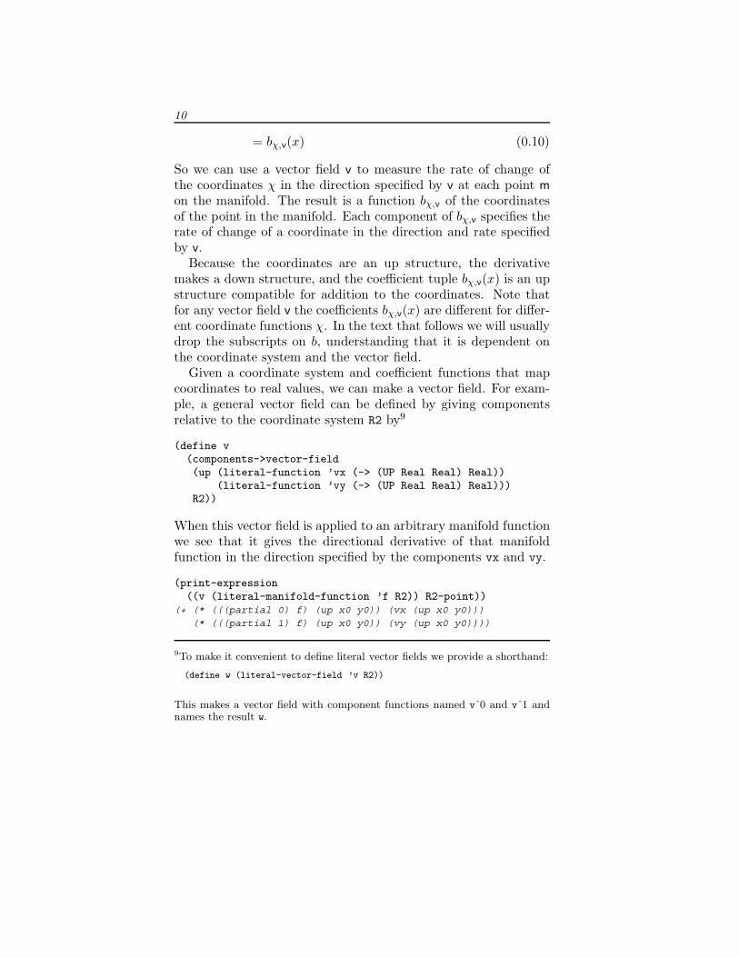
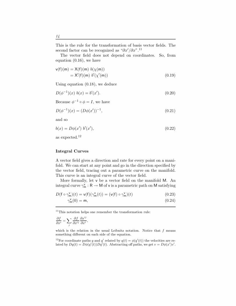
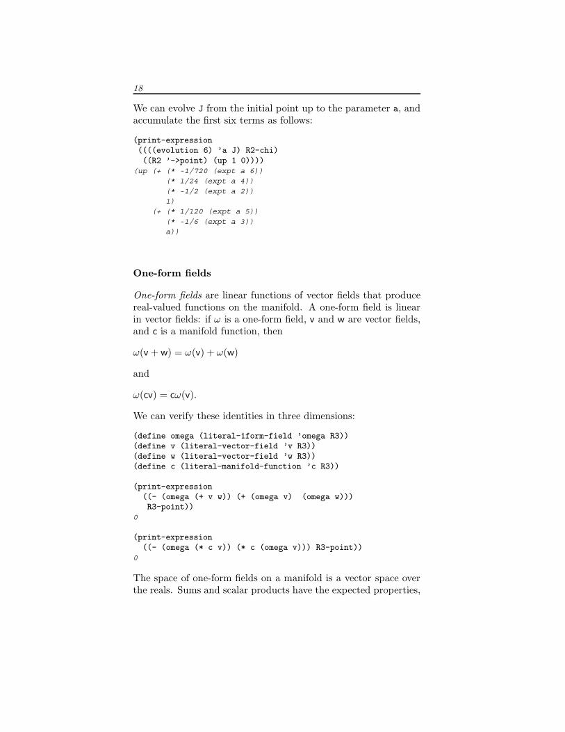
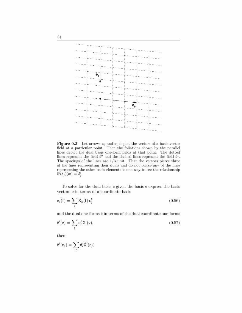
Figure 0.3 Let arrows e0 and e1 depict the vectors of a basis vectorfield at a particular point. Then the foliations shown by the parallellines depict the dual basis one-form fields at that point. The dottedlines represent the field e0 and the dashed lines represent the field e1.The spacings of the lines are 1/3 unit. That the vectors pierce threeof the lines representing their duals and do not pierce any of the linesrepresenting the other basis elements is one way to see the relationshipei(ej)(m) = δi

j .

To solve for the dual basis e given the basis e express the basisvectors e in terms of a coordinate basis

ej(f) =∑

k

Xk(f) ckj (0.56)

and the dual one-forms e in terms of the dual coordinate one-forms

ei(v) =∑

l

dil X

l(v), (0.57)

then

ei(ej) =∑

l

dilX

l(ej)

25

=∑

l

dilej(χl)

=∑

l

dil

∑k

Xk(χl)ckj

=∑kl

dilδ

lkc

kj

=∑

k

dikc

kj . (0.58)

Applying this at m we get

ei(ej)(m) = δij =

∑k

dik(m)ck

j (m). (0.59)

So the d coefficients can be determined from the c coefficents (es-sentially by matrix inversion).

The dual form fields can be used to determine the coefficients bof a vector field v relative to a basis e, by applying the dual basisform fields e to the vector field. Let

v(f) =∑

i

ei(f) bi. (0.60)

Then

ej(v) = bj . (0.61)

Define two general vector fields:

(define e0(+ (* (literal-manifold-function ’e0x R2) d/dx)

(* (literal-manifold-function ’e0y R2) d/dy)))

(define e1(+ (* (literal-manifold-function ’e1x R2) d/dx)

(* (literal-manifold-function ’e1y R2) d/dy)))

We use these as a vector basis and compute the dual:

(define e-vector-basis (down e0 e1))(define e-dual-basis

(vector-basis->dual e-vector-basis P2))

26

Then we can verify that they satisfy the dual relationship (equa-tion 0.39) by applying the dual basis to the vector basis:

(print-expression ((e-dual-basis e-vector-basis) m))(up (down 1 0) (down 0 1))

Note that the dual basis was computed relative to the polar coor-dinate system, showing how the resulting objects are independentof the coordinates in which they were expressed!

Or we can make a general vector field with this basis and thenpick out the coefficients by applying the dual basis:

(define v(* e-vector-basis

(up (literal-manifold-function ’bx R2)(literal-manifold-function ’by R2))))

(print-expression ((e-dual-basis v) R2-point))(up (bx (up x0 y0)) (by (up x0 y0)))

Commutators

The commutator of two vector fields is defined as

[v,w](f) = v(w(f)) − w(v(f)) (0.62)

The commutator of two coordinate basis fields is zero:

[Xi,Xj ](f) = Xi(Xj(f)) − Xj(Xi(f))= ∂i∂j(f ◦ χ−1) ◦ χ − ∂j∂i(f ◦ χ−1) ◦ χ

= 0, (0.63)

because the individual partial derivatives commute.The commutator of two vector fields is a vector field. Let v be

a vector field with coefficient function c = c ◦χ, and u be a vectorfield with coefficient function b = b ◦ χ, both with respect to thecoordinate basis X. Then

[u, v](f) = u(v(f)) − v(u(f))

= u(∑

i

Xi(f)ci) − v(∑

i

Xi(f)bi)

27

=∑

j

Xj(∑

i

Xi(f)ci)bj −∑

j

Xj(∑

i

Xi(f)bi)cj

=∑ij

[Xi,Xj ](f)cibj

+∑

i

Xi(f)∑

j

(Xj(ci)bj − Xj(bi)cj)

=∑

i

Xi(f)ai, (0.64)

where the coefficient function a of the commutator vector field is

ai =∑

j

(Xj(ci)bj − Xj(bi)cj

)= u(ci) − v(bi). (0.65)

We used the fact, shown above, that the commutator of two co-ordinate basis fields is zero.

We can check this formula for the commutator for the generalvector fields e0 and e1 in polar coordinates:

(let ((polar-vector-basis (basis->vector-basis polar-basis))(polar-dual-basis (basis->1form-basis polar-basis)))

(print-expression((- ((commutator e0 e1) f)

(* (- (e0 (polar-dual-basis e1))(e1 (polar-dual-basis e0)))

(polar-vector-basis f)))R2-point)))

0

Let e be a tuple of basis vector fields. The commutator of twobasis fields can be expressed in terms of the basis vector fields:

[ei, ej ](f) =∑

k

dkijek(f), (0.66)

where dkij are functions of m, called the structure constants for the

basis vector fields. The coefficients are

dkij = ek([ei, ej ]). (0.67)

28

Define the vector fields Jx, Jy, and Jz that generate rotationsabout the three rectangular axes in three dimensions:17

(define Jz (- (* x d/dy) (* y d/dx)))(define Jx (- (* y d/dz) (* z d/dy)))(define Jy (- (* z d/dx) (* x d/dz)))

(print-expression (((+ (commutator Jx Jy) Jz) g) R3-point))0(print-expression (((+ (commutator Jy Jz) Jx) g) R3-point))0(print-expression (((+ (commutator Jz Jx) Jy) g) R3-point))0

We see that

[Jx, Jy] = −Jz

[Jy, Jz ] = −Jx

[Jz, Jx] = −Jy. (0.68)

You can tell if a set of basis vector fields is a coordinate basis bycalculating the commutators. If they are non-zero, then the basisis not a coordinate basis. If they are zero then the basis vectorfields can be integrated to give the coordinate system.

Take a point 0 in M as the origin. Then, presuming [ei, ej ] = 0,the coordinates x of the point m in the coordinate system corre-sponding to the e basis satisfy18

m = Ex,e(0) = χ−1(x), (0.69)

where χ is the coordinate function being defined. Because theelements of e commute, the terms in the exponential can be simplyfactored into separate exponentials if needed.

17Using

(define R3 (rectangular 3))(instantiate-coordinates R3 ’(x y z))(define R3->R (-> (UP Real Real Real) Real))(define g

(compose (literal-function ’g R3->R)(R3 ’->coords)))

(define R3-point ((R3 ’->point) (up ’x ’y ’z)))

18Here x is an up-tuple structure of components, and e is down-tuple structureof basis vectors. The product of the two contracts to make a scaled vector.

29

Higher-Rank Forms

A one-form field applied to a vector field is a function on themanifold. We can extend this idea to k-form fields. A k-form fieldis an antisymmetric multilinear function that takes k vector fieldsand produces a function on the manifold.

Given two one-form fields ω and τ we can form a two-form fieldω ∧ τ as follows:

(ω ∧ τ)(v,w) = ω(v)τ(w) − ω(w)τ(v) (0.70)

In the special case where the one forms are the coordinate basisforms in rectangular coordinates the wedge of them measures theoriented area enclosed by a parallogram whose sides are describedby the vectors given as inputs:

(define R2 (rectangular 2))(instantiate-coordinates R2 ’(x y))(define R2-point ((R2 ’->point) (up ’x0 ’y0)))

(define v (+ (* ’a d/dx) (* ’b d/dy)))

(define w (+ (* ’c d/dx) (* ’d d/dy)))

(print-expression (((wedge dx dy) v w) R2-point))(+ (* a d) (* -1 b c))

More generally we can form the wedge of higher-rank forms.Let ω be a k-form field and τ be an l-form field. We can form ak + l-form field ω ∧ τ as follows:

ω ∧ τ =(k + l)!

k! l!Alt(ω ⊗ τ) (0.71)

where, if η is a m-form then

Alt(η)(v0, . . . , vm−1)

=1m!

∑σ∈Perm(m)

Parity(σ)η(vσ(0) , . . . , vσ(m−1)) (0.72)

and where

ω ⊗ τ(v0, . . . , vk−1, vk, . . . , vk+l−1)= ω(v0, . . . , vk−1)τ(vk, . . . , vk+l−1). (0.73)

30

The wedge product is associative, and thus we need not specifythe order of a multiple application.

The 3-form that is the wedge product of the rectangular coordinate-basis forms measures volumes:

(define R3 (rectangular 3))(instantiate-coordinates R3 ’(x y z))(define R3-point ((R3 ’->point) (up ’x0 ’y0 ’z0)))

(define u (+ (* ’a d/dx) (* ’b d/dy) (* ’c d/dz)))(define v (+ (* ’d d/dx) (* ’e d/dy) (* ’f d/dz)))(define w (+ (* ’g d/dx) (* ’h d/dy) (* ’i d/dz)))

(print-expression(((wedge dx dy dz) u v w) R3-point))

(+ (* a e i)(* -1 a f h)(* -1 b d i)(* b f g)(* c d h)(* -1 c e g))

This last expression is, if you don’t recognize it, the determinantof a 3 × 3 matrix:

(print-expression(- (((wedge dx dy dz) u v w) R3-point)

(determinant(matrix-by-rows (list ’a ’b ’c)

(list ’d ’e ’f)(list ’g ’h ’i)))))

0

In general, if the rank of a form is greater than the dimensionof the manifold then the form is identically zero.

Exterior Derivative

The intention of introducing the exterior derivative is to unifyall of the classical theorems of “vector analysis” into one unifiedStokes’s Theorem, which asserts that the integral of a form on the

31

boundary of a manifold is the integral of the exterior derivative ofthe form on the interior of the manifold:∫

∂Mω =

∫M

dω (0.74)

In order for this to work in a way independent of the coordinatesystem, the exterior derivative has to incorporate a Jacobian de-terminant to scale the line elements, area elements, or volumeelements.

As we have seen in equation (0.46), the differential of a functionon a manifold is a one-form field. If a function on a manifold isconsidered to be a form field of rank zero19 then the differentialoperator increases the rank of the form by one. We can generalizethis to k-form fields with the exterior derivative operation.

Consider a one-form ω. We define

dω(v1, v2) = v1(ω(v2)) − v2(ω(v1)) − ω([v1, v2]). (0.75)

The exterior derivative of a k-form field is a k + 1-form field,given by:20

dω(v0, . . . , vk)

=k∑

i=0

((−1)ivi(ω(v0, . . . , vi−1, vi+1, . . . , vk)) +

k∑j=i+1

(−1)i+jω([vi, vj ], v0, . . . , vi−1, vi+1, . . . , vj−1, vj+1, . . . , vk))

(0.76)

This formula is coordinate-system independent. This is the waywe compute the exterior derivative in our software.

19A manifold function f induces a form field f of rank 0 as follows:

f()(m) = f(m).

20See Spivak, Differential Geometry, Volume 1, p.289.

32

If the form field ω is represented in a coordinate basis

ω =n−1∑

i0=0,...,ik−1=0

ωi0,...,ik−1dxi0 ∧ · · · ∧ dxik−1 (0.77)

then the exterior derivative can be expressed as

dω =n−1∑

i0=0,...,ik−1=0

dωi0,...,ik−1 ∧ dxi0 ∧ · · · ∧ dxik−1 . (0.78)

Though this formula is expressed in terms of a coordinate basis,the result is independent of the choice of coordinate system.

We can test that the computation indicated by equation (0.76)is equivalent to the explicit computation indicated by equation (0.78)in three dimensions

(define R3 (rectangular 3))(instantiate-coordinates R3 ’(x y z))(define R3-point ((R3 ’->point) (up ’x0 ’y0 ’z0)))

with a general one-form field:

(define a (literal-manifold-function ’alpha R3))(define b (literal-manifold-function ’beta R3))(define c (literal-manifold-function ’gamma R3))

(define theta (+ (* a dx) (* b dy) (* c dz)))

The test will require two arbitrary vector fields

(define X (literal-vector-field ’X R3))(define Y (literal-vector-field ’Y R3))

(print-expression(((- (d theta)

(+ (wedge (d a) dx)(wedge (d b) dy)(wedge (d c) dz)))

X Y)R3-point))

0

33

We can also try a general 2-form field in three-dimensional space:Let

ω = ady ∧ dz + bdz ∧ dx + cdx ∧ dy, (0.79)

where a = α ◦ χ, b = β ◦ χ, c = γ ◦ χ, and α, β, and γ arereal-valued functions of three real arguments. As a program,

(define omega(+ (* a (wedge dy dz))

(* b (wedge dz dx))(* c (wedge dx dy))))

Here we need another vector field because our result will be a3-form field.

(define Z (literal-vector-field ’Z R3))

(print-expression(((- (d omega)

(+ (wedge (d a) dy dz)(wedge (d b) dz dx)(wedge (d c) dx dy)))

X Y Z)R3-point))

0

A form field ω that is the exterior derivative of another formfield ω = dθ is called exact. A form field whose exterior derivativeis zero is called closed.

Every exact form field is a closed form field, i.e. applying theexterior derivative operator twice always yields zero:

d2ω = 0. (0.80)

This is equivalent to the statement that partial derivatives withrespect to different variables commute.21

Consider the general one-form field θ defined on 3-dimensionalrectangular space. Two exterior derivatives of θ yields a 3-formfield, which must be proportional to the volume element.22 Itturns out to be zero:

21See Spivak, Calculus on Manifolds, p.92

22The dimension of the space of k-forms in an n-dimensional space is n−k+1.

34

(print-expression(((d (d theta)) X Y Z) R3-point))

0

Relationship to Vector Calculus:In three-dimensional Euclidean space the traditional vector deriva-tive operations are gradient, curl, and divergence. If x, y, z are theusual orthonormal vector basis, f a function on the space, and �vis a vector field on the space, then

grad(f) =∂f

∂xx +

∂f

∂yy +

∂f

∂zz

curl(�v) =(

∂vz

∂y− ∂vy

∂z

)x +

(∂vx

∂z− ∂vz

∂x

)y +

(∂vy

∂x− ∂vx

∂y

)x

div(�v) =∂vx

∂x+

∂vy

∂y+

∂vz

∂z

These vector calculus operations are subsumed by exterior deriva-tives of form fields, as follows. Let θ be a one-form field and let ωbe a two-form field:

θ = θxdx + θydy + θzdz

ω = ωxdy ∧ dz + ωydz ∧ dx + ωzdx ∧ dy

The exterior-derivative expressions corresponding to the vector-calculus expressions are:

df =∂f

∂xdx +

∂f

∂ydy +

∂f

∂zdz

dθ =(

∂θz

∂y− ∂θy

∂z

)dy ∧ dz +

(∂θx

∂z− ∂θz

∂x

)dz ∧ dx

+(

∂θy

∂x− ∂θx

∂y

)dx ∧ dy

dω =(

∂ωx

∂x+

∂ωy

∂y+

∂ωz

∂z

)dx ∧ dy ∧ dz.

Vector Integral Theorems:Green’s Theorem states that for an arbitrary compact set M ⊂ R2∫

∂M(α ◦ χ) dx + (β ◦ χ) dy =

∫M

((∂0β − ∂1α) ◦ χ) dx ∧ dy (0.81)

35

We can test this. By Stokes’s theorem, the integrands are relatedby an exterior derivative. First we need a plane.

(define R2 (rectangular 2))(instantiate-coordinates R2 ’(x y))(define R2-chi (R2 ’->coords))(define R2->R (-> (UP Real Real) Real))

We also need some vectors to test our forms:

(define v (literal-vector-field ’v R2))(define w (literal-vector-field ’w R2))

We can now test our integrands:

(define alpha (literal-function ’alpha R2->R))(define beta (literal-function ’beta R2->R))

(print-expression(((- (d (+ (* (compose alpha R2-chi) dx)

(* (compose beta R2-chi) dy)))(* (compose (- ((partial 0) beta)

((partial 1) alpha))R2-chi)

(wedge dx dy)))v w)R2-point))

0

We can also compute the integrands for the Divergence Theo-rem: For an arbitrary compact set M ⊂ R3 and a vector field w∫

Mdiv(w)dV =

∫∂M

w · n dA (0.82)

where n is the outward pointing normal to the surface ∂M . Again,the integrands should be related by an exterior derivative, if thisis an instance of Stokes’s Theorem.

Let

w = a∂

∂x+ b

∂

∂y+ c

∂

∂z(0.83)

We interpret w · ndA as the two-form

ω = ady ∧ dz + bdz ∧ dx + cdx ∧ dy, (0.84)

36

and div(w)dV as the three-form

dω =(

∂

∂xa +

∂

∂yb +

∂

∂zc

)dx ∧ dy ∧ dz. (0.85)

Let’s compute this to make sure it is true:

(define domega(* (+ (d/dx a) (d/dy b) (d/dz c))

(wedge dx dy dz)))

(print-expression(((- (d omega) domega) X Y Z) R3-point))

0

Over a Map

To deal with motion on manifolds we need to think about pathson manifolds and vectors along these paths. Vectors along pathsare not vector fields on the manifold because they are only definedon the path. And the path may even cross itself, which would givemore than one vector at a point. Here we introduce the conceptof over a map, which solves this problem.23

Let μ map points n in the manifold N to points m in the man-ifold M. A vector over the map μ takes directional derivativesof functions on M at points m = μ(n). The vector over the mapapplied to the function on M is a function on N.

Let v be a vector field on M, and f a function on M. Then

vμ(f) = v(f) ◦ μ, (0.86)

is a vector over the map μ. Note that vμ(f) is a function on N,not M:

vμ(f)(n) = v(f)(μ(n)). (0.87)

We can implement this definition as:

23see Bishop and Goldberg, Tensor Analysis on Manifolds.

37

(define ((vector-field-over-map mu:N->M) v-on-M)(procedure->vector-field(lambda (f-on-M)(compose (v-on-M f-on-M) mu:N->M))))

Given a one-form ω, the one-form over the map μ is constructedas follows:

ωμ(vμ)(n) = ω(u)(μ(n)), where u(f)(m) = vμ(f)(n). (0.88)

The object u is not really a vector field on M even though we havegiven it that shape so that the dual vector can apply to it; u(f) isonly evaluated at images m = μ(n) of points n in N. If we weredefining u as a vector field we would need the inverse of μ to findthe point n = μ−1(m), but this is not required to define the objectu in a context where there is already an m associated with the nof interest. To extend this idea to k-forms, we carry each vectorargument over the map.

The procedure that implements u, that is, that makes a vectorfield over the map μ : N → M appear as a vector field on M is

(define (vector-field-over-map->vector-field V-over-mu n)(procedure->vector-field(lambda (f)(lambda (m) ((V-over-mu f) n)))))

Using this, the procedure that constructs a k-form over the mapfrom a k-form is:

(define ((form-field-over-map mu:N->M) w-on-M)(let ((k (get-rank w-on-M)))(procedure->nform-field(lambda vectors-over-map

(lambda (n)((apply w-on-M

(map (lambda (V-over-mu)(vector-field-over-map->vector-fieldV-over-mu n))

vectors-over-map))(mu:N->M n))))

k)))

38

Let e be a tuple of basis vector fields, and e be the tuple of basisone-forms that is dual to e:

ei(ej)(m) = δij . (0.89)

The basis vectors over the map, eμ, are particular cases of vectorsover a map:

eμ(f) = e(f) ◦ μ. (0.90)

And the elements of the dual basis over the map, eμ, are particularcases of one-forms over the map. The basis and dual basis overthe map satisfy

eiμ(eμ

j )(n) = δij . (0.91)

For example, let μ map the time line to the unit sphere. Weuse colatitude θ and longitude φ as coordinates on the sphere

(define sphere (S2 1)) ; sphere with R=1(instantiate-coordinates sphere ’(theta phi))(define sphere-basis (coordinate-system->basis sphere))

and let t be the coordinate of the real line.

(instantiate-coordinates the-real-line ’t)

A general path on the sphere is:

(define mu(compose (sphere ’->point)

(up (literal-function ’alpha)(literal-function ’beta))

(the-real-line ’->coords)))

The basis over the map is constructed from the basis on the sphere:

(define sphere-basis-over-mu(basis->basis-over-map mu sphere-basis))

(define h(compose (literal-function ’h R2->R)

(sphere ’->coords)))

39

(print-expression(((basis->vector-basis sphere-basis-over-mu) h)((the-real-line ’->point) ’t0)))

(down(((partial 0) h) (up (alpha t0) (beta t0)))(((partial 1) h) (up (alpha t0) (beta t0))))

The basis vectors over the map compute derivatives of the functionh evaluated on the path at the given time.

We can check that the dual basis over the map does the correctthing

(print-expression(((basis->1form-basis sphere-basis-over-mu)(basis->vector-basis sphere-basis-over-mu))((the-real-line ’->point) ’t0)))

(up (down 1 0) (down 0 1))

Pullback of a Function:The pullback of a function f on M over the map μ is defined as

μ∗f = f ◦ μ. (0.92)

This allows us to take a function defined on M and use it to definea new function on N.

For example, the integral curve of v evolved for time t as afunction of the initial manifold point m generates a map φv

t of themanifold onto itself. This is a simple Currying of the integral curveof v from m as a function of time: φv

t (m) = γvm(t). The evolution

of the function f along an integral curve, equation (0.34), can bewritten in terms of the pullback over φv

t :

(Et,vf)(m) = f(φvt (m)) = ((φv

t )∗f)(m). (0.93)

Pushforward of a Vector Field:We can also pushforward a vector field over the map μ. The push-forward takes a vector field v defined on N. The result takesdirectional derivatives of functions on M at a place determined bya point in M:

μ∗v(f)(m) = v(μ∗f)(μ−1(m)) = v(f ◦ μ)(μ−1(m)). (0.94)

40

We can pushforward a vector field over the map generated by anintegral curve, because the inverse is always available.24

((φvt )∗v)(f)(m) = v((φv

t )∗f)(φv

−t(m)) = v(f ◦ φvt )(φ

v−t(m)). (0.95)

Differential of a Map:For more general maps the pushforward of a vector field is notvery useful because it requires inverting the map μ. A more usefulconstruct in this context is the differential of the map

dμ(v)(f)(n) = v(μ∗f)(n) = v(f ◦ μ)(n), (0.96)

which takes its argument in the source manifold N. The differen-tial of a map applied to a vector yields a vector over the map. Aprocedure to compute the differential is:

(define (((differential mu) v) f)(v (compose f mu)))

The nomenclature of this subject is confused. The “differentialof a map” between manifolds dμ takes one more argument thanthe “differential of a real-valued function on a manifold” df, butthe two are related:

dμ(v)(I)(n) = dμ(v)(n), (0.97)

where the target manifold of μ is the reals and I is the identityfunction on the reals.

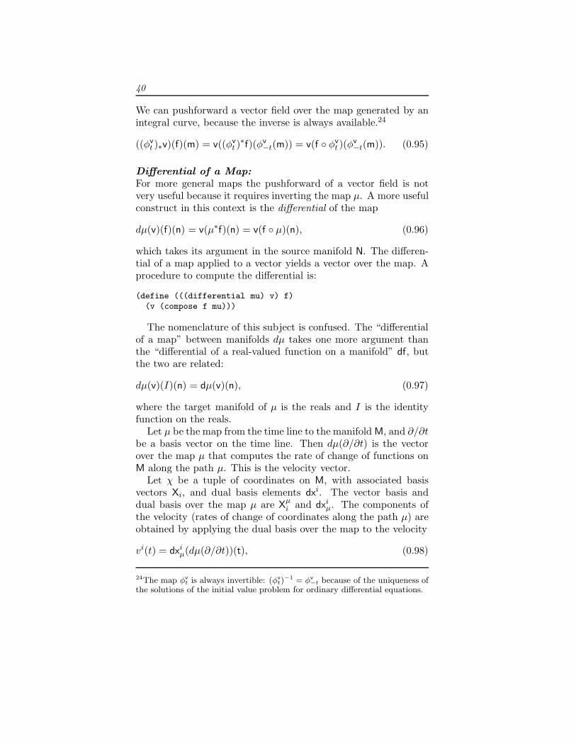
Let μ be the map from the time line to the manifold M, and ∂/∂tbe a basis vector on the time line. Then dμ(∂/∂t) is the vectorover the map μ that computes the rate of change of functions onM along the path μ. This is the velocity vector.

Let χ be a tuple of coordinates on M, with associated basisvectors Xi, and dual basis elements dxi. The vector basis anddual basis over the map μ are Xμ

i and dxiμ. The components of

the velocity (rates of change of coordinates along the path μ) areobtained by applying the dual basis over the map to the velocity

vi(t) = dxiμ(dμ(∂/∂t))(t), (0.98)

24The map φvt is always invertible: (φv

t)−1 = φv

−t because of the uniqueness ofthe solutions of the initial value problem for ordinary differential equations.

41

where t is the coordinate for the point t.For example, the velocities on a sphere are

(print-expression(((basis->1form-basis sphere-basis-over-mu)((differential mu) d/dt))((the-real-line ’->point) ’t0)))

(up ((D alpha) t0) ((D beta) t0)))

as expected.

Pullback of a Vector Field:Given a vector field v on manifold M we can pullback the vectorfield through the map μ : N → M as follows:

μ∗v = (μ−1)∗v, (0.99)

or

μ∗v(f) = (v(f ◦ μ−1)) ◦ μ (0.100)

This may be useful when the map is invertible, as in the flowgenerated by a vector field.

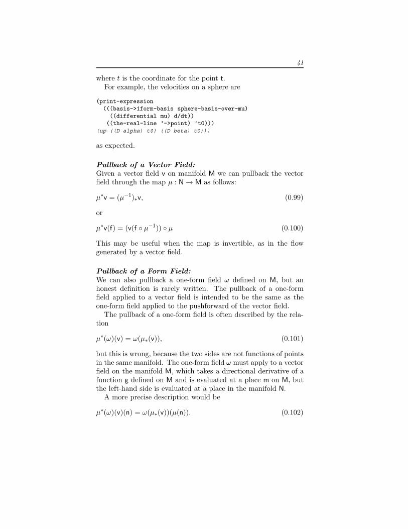
Pullback of a Form Field:We can also pullback a one-form field ω defined on M, but anhonest definition is rarely written. The pullback of a one-formfield applied to a vector field is intended to be the same as theone-form field applied to the pushforward of the vector field.

The pullback of a one-form field is often described by the rela-tion

μ∗(ω)(v) = ω(μ∗(v)), (0.101)

but this is wrong, because the two sides are not functions of pointsin the same manifold. The one-form field ω must apply to a vectorfield on the manifold M, which takes a directional derivative of afunction g defined on M and is evaluated at a place m on M, butthe left-hand side is evaluated at a place in the manifold N.

A more precise description would be

μ∗(ω)(v)(n) = ω(μ∗(v))(μ(n)). (0.102)

42

Although this is accurate, it may not be effective, because com-puting the pushforward requires the inverse of the map μ. Again,this is available when the map is the flow generated by a vectorfield.

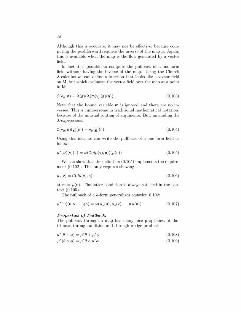
In fact it is possible to compute the pullback of a one-formfield without having the inverse of the map. Using the Churchλ-calculus we can define a function that looks like a vector fieldon M, but which evaluates the vector field over the map at a pointin N:

C(vμ, n) = λ(g)(λ(m)vμ(g)(n)). (0.103)

Note that the bound variable m is ignored and there are no in-verses. This is cumbersome in traditional mathematical notation,because of the unusual routing of arguments. But, unwinding theλ-expressions:

C(vμ, n)(g)(m) = vμ(g)(n). (0.104)

Using this idea we can write the pullback of a one-form field asfollows:

μ∗(ω)(v)(n) = ω(C(dμ(v), n))(μ(n)) (0.105)

We can show that the definition (0.105) implements the require-ment (0.102). This only requires showing

μ∗(v) = C(dμ(v), n), (0.106)

at m = μ(n). The latter condition is always satisfied in the con-text (0.105).

The pullback of a k-form generalizes equation 0.102:

μ∗(ω)(u, v, . . .)(n) = ω(μ∗(u), μ∗(v), . . .)(μ(n)). (0.107)

Properties of Pullback:The pullback through a map has many nice properties: it dis-tributes through addition and through wedge product:

μ∗(θ + φ) = μ∗θ + μ∗φ (0.108)μ∗(θ ∧ φ) = μ∗θ ∧ μ∗φ (0.109)

43

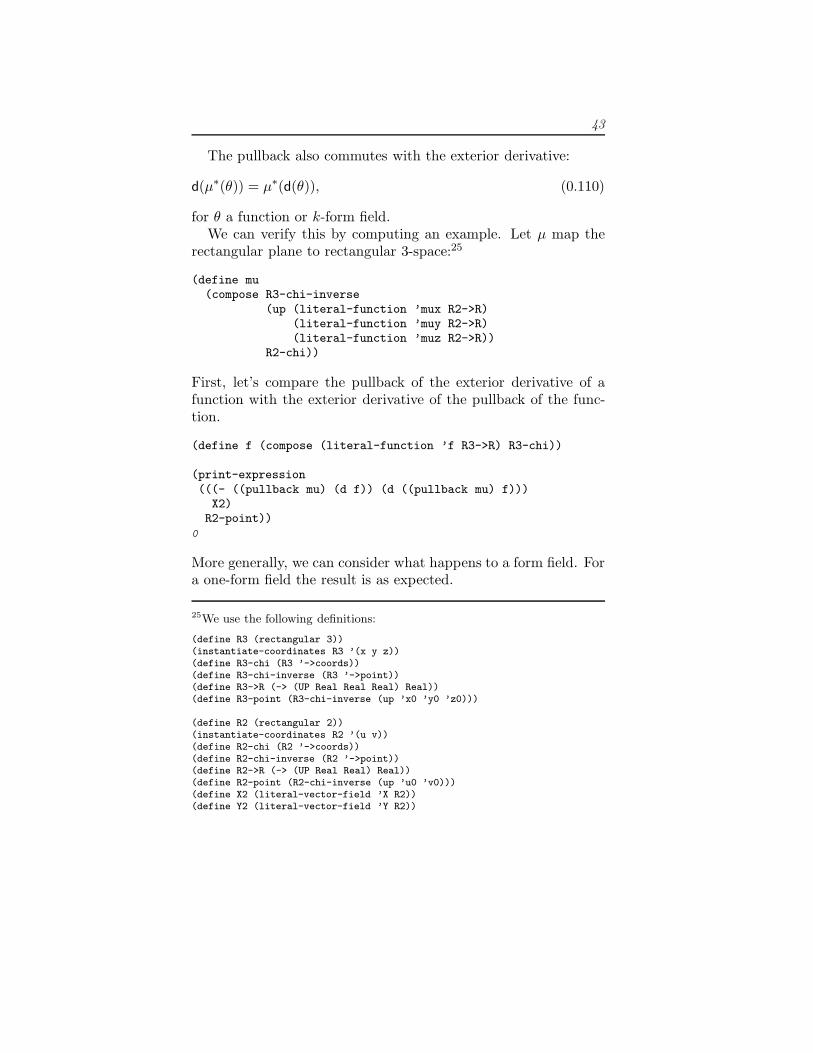
The pullback also commutes with the exterior derivative:

d(μ∗(θ)) = μ∗(d(θ)), (0.110)

for θ a function or k-form field.We can verify this by computing an example. Let μ map the

rectangular plane to rectangular 3-space:25

(define mu(compose R3-chi-inverse

(up (literal-function ’mux R2->R)(literal-function ’muy R2->R)(literal-function ’muz R2->R))

R2-chi))

First, let’s compare the pullback of the exterior derivative of afunction with the exterior derivative of the pullback of the func-tion.

(define f (compose (literal-function ’f R3->R) R3-chi))

(print-expression(((- ((pullback mu) (d f)) (d ((pullback mu) f)))

X2)R2-point))

0

More generally, we can consider what happens to a form field. Fora one-form field the result is as expected.

25We use the following definitions:

(define R3 (rectangular 3))(instantiate-coordinates R3 ’(x y z))(define R3-chi (R3 ’->coords))(define R3-chi-inverse (R3 ’->point))(define R3->R (-> (UP Real Real Real) Real))(define R3-point (R3-chi-inverse (up ’x0 ’y0 ’z0)))

(define R2 (rectangular 2))(instantiate-coordinates R2 ’(u v))(define R2-chi (R2 ’->coords))(define R2-chi-inverse (R2 ’->point))(define R2->R (-> (UP Real Real) Real))(define R2-point (R2-chi-inverse (up ’u0 ’v0)))(define X2 (literal-vector-field ’X R2))(define Y2 (literal-vector-field ’Y R2))

44

(define theta (literal-1form-field ’theta R3))

(print-expression(((- ((pullback mu) (d theta)) (d ((pullback mu) theta)))

X2 Y2)R2-point))

0

Lie Derivative

The Lie derivative is a measure of how things change along theintegral curves of a vector field. The Lie derivative of any objectis another object of the same kind. The form of the Lie derivativedepends on the kind of object that is being differentiated. How-ever, we will see that there are uniform ways of specifying the Liederivative.26

Functions:The simplest kind of object is a function on the manifold. Letf be a function on the manifold, and φv

t (m) be the point alongthe integral curve of the vector field v beginning at m, advancedfor interval t. Then the Lie derivative of f with respect to v is afunction defined by:

Lv(f)(m) = limt→0

(((φv

t )∗f)(m) − f(m)

t

)(0.111)

= limt→0

(f(φv

t (m)) − f(m)t

)= v(f)(m) (0.112)

So the Lie derivative of a function is just the derivative of thefunction along the integral curve of v.

Vector Fields:The Lie derivative of a vector field y with respect to a vector fieldv is a vector field that is defined by its behavior when appliedto an arbitrary manifold function f. The Lie derivative compares

26Thanks to Will Farr, who showed us a unified framework for understandingLie derivatives.

45

the pullback of the vector field y along the integral curves of thevector field v with the original vector field y:

Lvy(f)(m) = limt→0

(((φv

t )∗y)(f)(m) − y(f)(m)t

)(0.113)

= limt→0

(((φv−t)∗y)(f)(m) − y(f)(m)

t

)(0.114)

= limt→0

((φv

t )∗(y((φv−t)∗f))(m) − y(f)(m)t

)(0.115)

= limt→0

(y((φv−t)

∗f)(m) + tv(y((φv−t)∗f))(m) − y(f)(m)

t

)= lim

t→0(v(y((φv

−t)∗f))(m)) − y(v(f))(m)

= v(y(f))(m) − y(v(f))(m) (0.116)= [v, y](f)(m) (0.117)

So the Lie derivative of one vector field with respect to anotheris just their commutator. Note that the tricky step (0.115) in thederivation above depends on Hadamard’s Lemma,27 which allowsus to deduce that: (φv

t )∗g = g ◦ φv

t = g + tv(g) + O(t2). We applythis in equation (0.115), defining g = y((φv−t)

∗f).The Lie derivative of a vector field can also be seen as a com-

parison of the advance of the application of the vector field to thefunction with the application of the vector field to the advance ofthe function:

Lvy(f)(m) = limt→0

((φv

t )∗(y(f))(m) − y((φvt )∗f)(m)

t

)= lim

t→0

(y(f)(φv

t (m)) − y(f ◦ φvt )(m)

t

)(0.118)

We can write this as a derivative28

Lvy(f)(m) = Dg(0), (0.119)

27See Theodore Frankel, The Geometry of Physics, Cambridge UniversityPress 1997, pp. 126–127.

28Using L’Hospital’s rule.

46

with

g(t) = y(f)(φvt (m)) − y(f ◦ φv

t )(m). (0.120)

The derivative of the first term of g is of the form of the deriva-tive of a function h = y(f) along the integral curve of v starting atm, so this term is just v(y(f))(m).

Let h(t) = y(f ◦ φvt )(m), the second term of g(t). We need to

calculate Dh(0). Now,29

(f ◦ φvt ) = f + t v(f) + · · · , (0.121)

and since y is linear

y(f ◦ φvt ) = y(f) + t y(v(f)) + · · · . (0.122)

So Dh(0) = y(v(f))(m). Combining these two terms we get thecommutator: so

Lvy(f) = [v, y](f), (0.123)

as before.

Exponentiating Lie Derivatives:We can exponentiate the Lie derivative and apply it to a vectorfield:

eLvy = y + Lvy +12Lv

2y + · · ·

= y + [v, y] +12[v, [v, y]] + · · · (0.124)

Consider a simple case. We advance the coordinate basis vector∂/∂y by an angle a around the circle. Let J = x ∂/∂y − y ∂/∂x,the circular vector field. We recall

(define J (- (* x d/dy) (* y d/dx)))

We can apply the exponential of Lie derivative with respect to Jto ∂/∂y. We examine how the result affects a general function onthe manifold:

29Again, by Hadamard’s Lemma.

47

(series:for-each print-expression((((exp (* ’a (Lie-derivative J))) d/dy)(literal-manifold-function ’f R2))((R2 ’->point) (up 1 0)))5)

(((partial 1) f) (up 1 0))(* a (((partial 0) f) (up 1 0)))(* -1/2 (expt a 2) (((partial 1) f) (up 1 0)))(* -1/6 (expt a 3) (((partial 0) f) (up 1 0)))(* 1/24 (expt a 4) (((partial 1) f) (up 1 0)));Value: ...

Apparently the result is

exp(La (x ∂/∂y−y ∂/∂x)

) ∂

∂y= sin(a)

∂

∂x+ cos(a)

∂

∂y. (0.125)

Form fields:We can also define the Lie derivative of a form field. Consider aone-form field ω. Its Lie derivative with respect to a vector fieldv is a one-form field defined by its action on an arbitrary vectorfield y:

Lvω(y)(m) = limt→0

((φv

t )∗ω(y)(m) − ω(y)(m)t

)(0.126)

= limt→0

(ω((φv

t )∗y)(φvt (m)) − ω(y)(m)

t

)= lim

t→0

(v(ω(φv

t )∗y)(m) +ω((φv

t )∗y)(m) − ω(y)(m)t

)= v(ω(y))(m) − ω(Lvy)(m) (0.127)

The Lie derivative of a k-form field ω with respect to a vectorfield v is a k-form field that is defined by its behavior when appliedto k arbitrary vector fields w0, . . . ,wk−1. Using the fact that thepullback of a k-form is the form applied to the pushforward ofall its arguments evaluated at the right place, we can generalizethe derivation for one-form fields to k-form fields, by the followingformula:

Lvω(w0, . . . ,wk−1)

= v(ω(w0, . . . ,wk−1)) −k−1∑i=0

ω(w0, . . . ,Lvwi, . . . ,wk−1)(0.128)

48

Uniform InterpretationNotice that in each case, the Lie derivative can be written ina form reminiscent of an elementary derivative. Consider equa-tions (0.111), (0.113), and (0.126). Each is a limit of a quotientof a difference of a pullback of a thing and the thing. If we under-stand the pullback as the advance along the integral curve thenthis is the ordinary derivative.

Another uniform way of writing the Lie derivative is the vectorfield applied to the composite function minus the function appliedto the Lie derivative of its arguments. For a function, the Liederivative is just

Lv(f) = v(f). (0.129)

For a vector field (see equation 0.116)

Lvy(f) = v(y(f)) − y(Lv(f)). (0.130)

For a one-form field (see equation 0.127)

Lvω(y) = v(ω(y)) − ω(Lvy). (0.131)

The generalization for k-form fields is just equation (0.128).

Properties of the Lie Derivative:For any k-form field ω and any vector field v the exterior derivativecommutes with the Lie derivative with respect to the vector field:

Lv(dω) = d(Lvω) (0.132)

We can verify this in three-dimensional rectangular space for ourgeneral one form:

(define V (literal-vector-field ’V R3))

(print-expression(((- ((Lie-derivative V) (d theta))

(d ((Lie-derivative V) theta)))X Y)R3-point))

0

and for the general 2-form:

49

(print-expression(((- ((Lie-derivative V) (d omega))

(d ((Lie-derivative V) omega)))X Y Z)R3-point))

0

The Lie derivative satisfies a another nice elementary relation-ship. If v and w are two vector fields then

[Lv,Lw] = L[v,w]. (0.133)

Again, for our general one-form θ:

(print-expression((((- (commutator (Lie-derivative X) (Lie-derivative Y))

(Lie-derivative (commutator X Y)))theta)Z)R3-point))

0

and for the two-form ω:

(print-expression((((- (commutator (Lie-derivative X) (Lie-derivative Y))

(Lie-derivative (commutator X Y)))omega)Z V)R3-point))

0

Interior Product

There is a simple, but useful operation available between vectorfields and form fields called interior product. This is the substitu-tion of a vector field v into the first argument of an p-form field ωto produce an p − 1-form field:

(ivω)(v1, . . . vp−1) = ω(v, v1, . . . vp−1) (0.134)

50

There is a rather nice identity for the Lie derivative in terms ofthe interior product called Cartan’s formula:

Lvω = iv(dω) + d(ivω) (0.135)

We can verify Cartan’s formula in a simple case with a program:

(define R3 (rectangular 3))(instantiate-coordinates R3 ’(x y z))

(define X (literal-vector-field ’X R3))(define Y (literal-vector-field ’Y R3))(define Z (literal-vector-field ’Z R3))

(define alpha (literal-manifold-function ’alpha R3))(define beta (literal-manifold-function ’beta R3))(define gamma (literal-manifold-function ’gamma R3))

(define omega(+ (* alpha (wedge dx dy))

(* beta (wedge dy dz))(* gamma (wedge dz dx))))

(define ((L1 X) omega)(+ ((interior-product X) (d omega))

(d ((interior-product X) omega))))

(print-expression((- (((Lie-derivative X) omega) Y Z)

(((L1 X) omega) Y Z))((R3 ’->point) (up ’x0 ’y0 ’z0))))

0

Note that iv ◦ iu + iu ◦ iv = 0. One consequence of this is thativ ◦ iv = 0.

Covariant Derivative of Vector Fields

Vectors at the same manifold point can be directly compared,but vectors at different points cannot. Parallel transport allowsvectors at different points to be compared by transporting them tothe same place. To define parallel transport, and the associatedidea of covariant derivative, we need to introduce a connection.The connection cannot be derived, and there is freedom in the

51

choice of a connection. If there is a metric, then there is a specialconnection determined by it.

The covariant derivative with respect to the vector field u ofthe vector field v is

(∇uv)(f) =∑

i

ei(f)

(u(ei(v)) +

∑j

ωij(u)ej(v)

)

=∑

i

ei(f)

(u(vi) +

∑j

ωij(u)vj

)= e(f)(u(v) + ω(u)v), (0.136)

where ω is a structure-valued one-form and ωij is a one-form for

each selector i and j. These one-forms are called the Cartan one-forms, or the connection one-forms. The Cartan forms are definedwith respect to the basis e and its dual e. In these expressions vis the structure of coefficient manifold functions for the vector vwith respect to the basis e, and vi is a component of v. Thoughthe covariant derivative is expressed with respect to a basis, theresult is independent of the basis.

As a program, the covariant derivative is:30

30This program is slightly incomplete, for two reasons. It must construct avector field, and it must make a differential operator. The full program is abit longer:

(define (covariant-derivative Cartan)(let ((basis (Cartan->basis Cartan))

(Cartan-forms (Cartan->forms Cartan)))(let ((vector-basis (basis->vector-basis basis))

(1form-basis (basis->1form-basis basis)))(define (nabla X)(define (nabla X V)

(let ((v-components (1form-basis V)))(let ((deriv-components

(+ (X v-components)(* (Cartan-forms X) v-components))))

(define (the-derivative f)(* (vector-basis f) deriv-components))

(procedure->vector-field the-derivative‘((nabla ,(diffop-name X)) ,(diffop-name V))))))

(procedure->vector-field nabla X‘(nabla ,(diffop-name X))))

nabla)))

52

(define ((((covariant-derivative Cartan) X) V) f)(let ((basis (Cartan->basis Cartan))

(Cartan-forms (Cartan->forms Cartan)))(let ((vector-basis (basis->vector-basis basis))

(1form-basis (basis->1form-basis basis)))(let ((v-components (1form-basis V)))(* (vector-basis f)

(+ (X v-components)(* (Cartan-forms X) v-components)))))))

The Cartan forms can be constructed from the dual basis one-forms:

ωij(v)(m) =

∑k

Γijk(m) ek(v)(m). (0.137)

The connection coefficient functions Γijk are sometimes called the

Christoffel symbols.31 Making use of the structures, the Cartanforms are

ω(v) = Γ e(v). (0.138)

Conversely, the Christoffel coefficients may be obtained from theCartan forms

Γijk = ωi

j(ek). (0.139)

The covariant derivative is independent of the coordinate sys-tem. We can show this in a simple case, using rectangular and

31This terminology may be restricted to the case in which the basis is a coor-dinate basis.

53

polar coordinates in the plane.32 The Christoffel coefficients forrectangular coordinates in a (flat) plane are all zero:33

(define rectangular-Christoffel(make-Christoffel(let ((zero (lambda (m) 0)))(down (down (up zero zero)

(up zero zero))(down (up zero zero)

(up zero zero))))rectangular-basis))

The Christoffel coefficients for polar coordinates on the planeare:34

(define polar-Christoffel(make-Christoffel(let ((zero (lambda (m) 0)))(down (down (up zero zero)

(up zero (/ 1 r)))(down (up zero (/ 1 r))

(up (* -1 r) zero))))polar-basis))

From these we can make the Cartan forms in both coordinatesystems:35

32We will need a few definitions:

(define R2 (rectangular 2))(instantiate-coordinates R2 ’(x y))(define rectangular-basis (coordinate-system->basis R2))(define R2-chi (R2 ’->coords))(define R2-chi-inverse (R2 ’->point))

(define P2 (polar/cylindrical 2))(instantiate-coordinates P2 ’(r theta))(define polar-basis (coordinate-system->basis P2))(define P2-chi (P2 ’->coords))(define P2-chi-inverse (P2 ’->point))

33Since the Christoffel coefficients are basis dependent they are packaged withthe basis.

34We will derive these later.

35The code for making the Cartan forms is as follows:

54

(define rectangular-Cartan(Christoffel->Cartan rectangular-Christoffel))

(define polar-Cartan(Christoffel->Cartan polar-Christoffel))

The vector field Jz generates a rotation in the plane (the sameas J). The covariant derivative with respect to ∂/∂x of Jz appliedto an arbitrary manifold function is:

(define f(compose (literal-function ’f-rect R2->R) R2-chi))

(print-expression(((((covariant-derivative rectangular-Cartan) d/dx)

J)f)R2-point))

(((partial 1) f-rect) (up x0 y0))

Note that this is the same thing as ∂/∂y applied to the function:

(print-expression ((d/dy f) R2-point))(((partial 1) f-rect) (up x0 y0))

In rectangular coordinates, where the Christoffel coefficients arezero, the covariant derivative ∇uv is the vector whose coefficentsare obtained by applying u to the coefficients of v. Here, onlyone coefficient of Jz depends on x, the coefficient of ∂/∂y, and itdepends linearly on x. So ∇∂/∂xJz = ∂/∂y.

Note that we get the same answer if we use polar coordinatesto compute the covariant derivative:

(print-expression(((((covariant-derivative polar-Cartan) d/dx)

J)f)R2-point))

(((partial 1) f-rect) (up x0 y0))

(define (Christoffel->Cartan Christoffel)(let ((basis (Christoffel->basis Christoffel))

(Christoffel-symbols (Christoffel->symbols Christoffel)))(make-Cartan(* Christoffel-symbols (basis->1form-basis basis))basis)))

55

’ν

d/dy

d/dx

ν

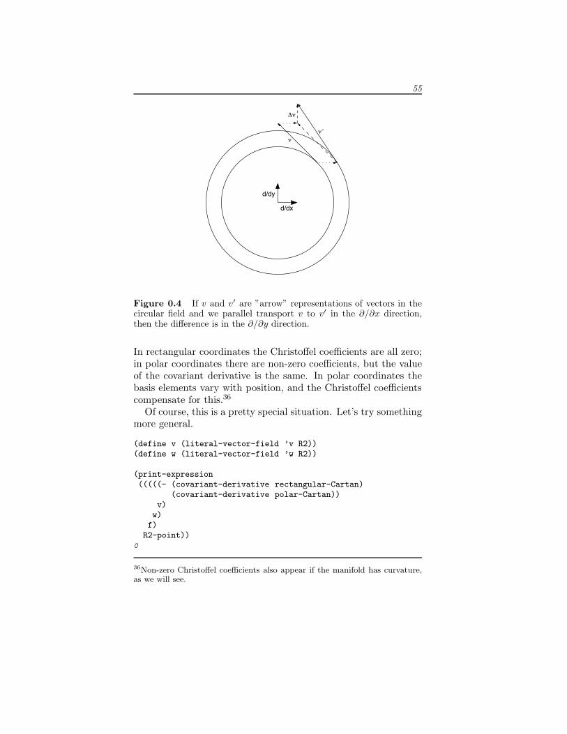
Δν

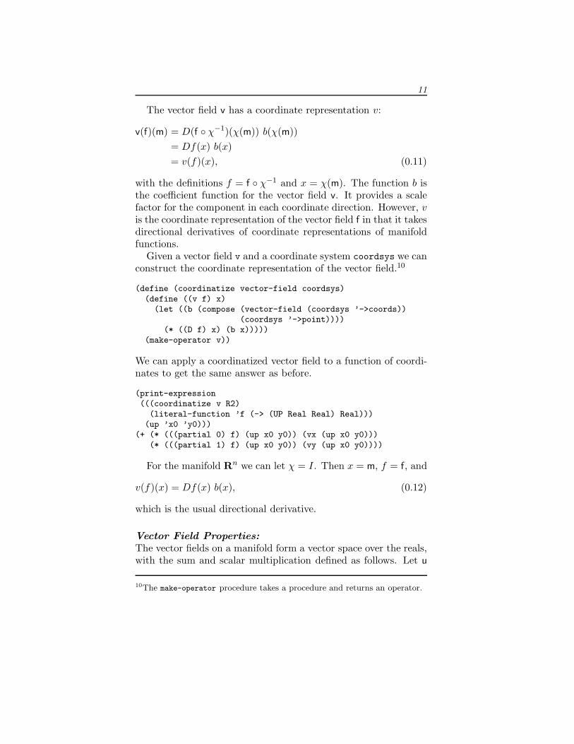
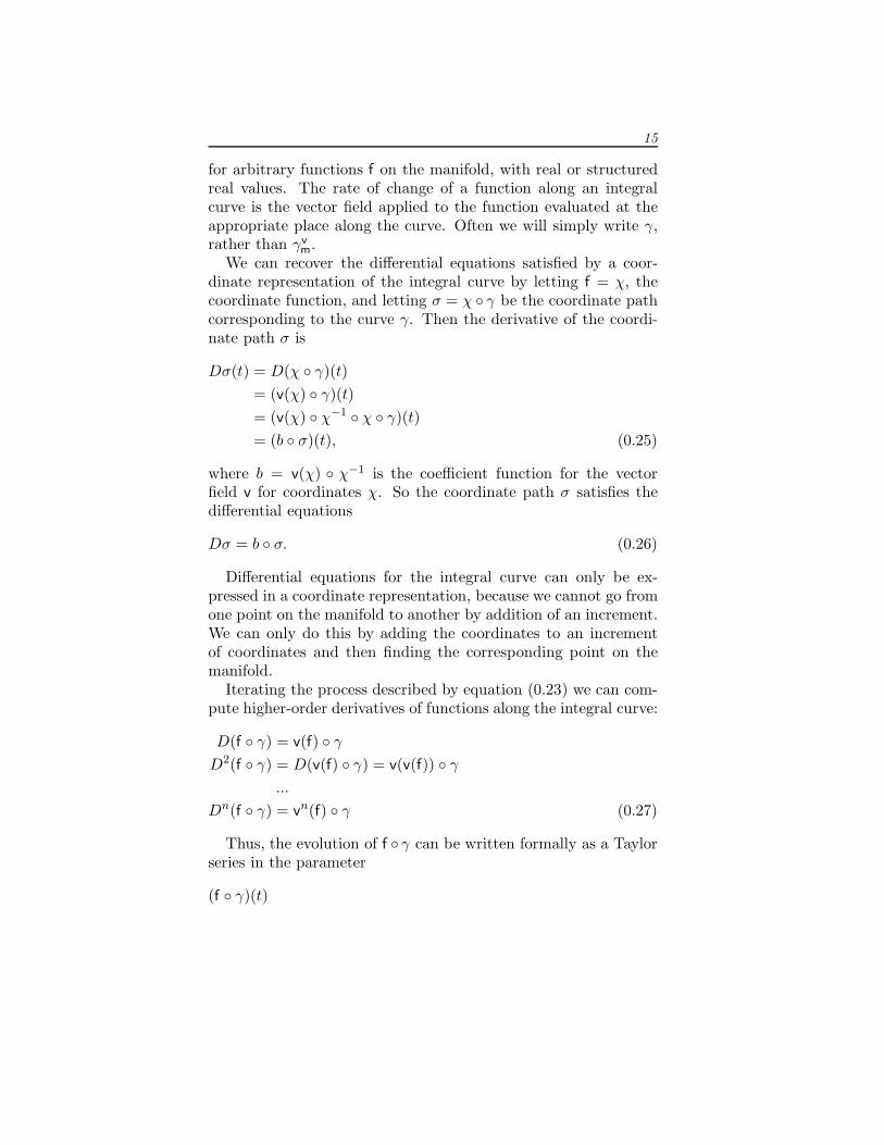
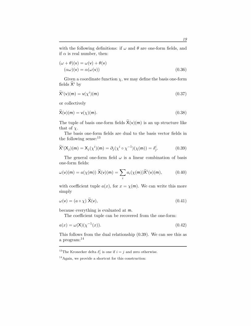
Figure 0.4 If v and v′ are ”arrow” representations of vectors in thecircular field and we parallel transport v to v′ in the ∂/∂x direction,then the difference is in the ∂/∂y direction.

In rectangular coordinates the Christoffel coefficients are all zero;in polar coordinates there are non-zero coefficients, but the valueof the covariant derivative is the same. In polar coordinates thebasis elements vary with position, and the Christoffel coefficientscompensate for this.36

Of course, this is a pretty special situation. Let’s try somethingmore general.

(define v (literal-vector-field ’v R2))(define w (literal-vector-field ’w R2))

(print-expression(((((- (covariant-derivative rectangular-Cartan)

(covariant-derivative polar-Cartan))v)w)f)R2-point))

0

36Non-zero Christoffel coefficients also appear if the manifold has curvature,as we will see.

56

Parallel Transport

Given a connection we can define the operation of parallel trans-port of a vector along a path. Let γ be a path, a map from thereal line to the manifold M. We would like to parallel transportw, a vector over the map γ, along the path γ.

We can specify w in terms of a basis over the map eγ as follows:

w(f)(t) =∑

i

eγi (f)(t)ci(t) = (eγ(f) c)(t). (0.140)

The coefficients c are functions on the time line and have struc-tured values that are compatible for contraction with a basis onM.

The covariant derivative is expressed with respect to a basisand a set of Cartan forms. If we replace these with a basis overa map and the Cartan forms over the map then we get a covari-ant derivative over the map. The resulting covariant derivative isindependent of the particular basis chosen, but now depends onthe map, notated ∇γ . The construction of the basis over the mapwas shown previously. The Cartan forms over the map are thepullback over the map of the Cartan forms: ωγ = γ∗ω.

The equation governing the parallel transport of w is

∇γ∂/∂tw = 0. (0.141)

Let’s figure out what this equation is for transport of an arbitraryvector w along an arbitrary path γ on a sphere. We start byconstructing the necessary manifolds.

(instantiate-coordinates the-real-line ’t)

(define M (rectangular 2))(instantiate-coordinates M ’(theta phi))(define M-basis (coordinate-system->basis M))

We specify a connection by giving the Christoffel symbols.37

37We will show how to get these Christoffel symbols from a metric.

57

(define G-S2-1(make-Christoffel(let ((zero (lambda (point) 0)))(down (down (up zero zero)

(up zero (/ 1 (tan theta))))(down (up zero (/ 1 (tan theta)))

(up (- (* (sin theta) (cos theta))) zero))))M-basis))

Next, we need the path γ, which we represent as a map from thereal line to M , and w, the parallel-transported vector over themap:

(define gamma:N->M(compose (M ’->point)

(up (literal-function ’alpha)(literal-function ’beta))

(the-real-line ’->coords)))

where alpha is the colatitude and beta is the longitude.

(define basis-over-gamma(basis->basis-over-map gamma:N->M M-basis))

(define w(basis-components->vector-field(up (compose (literal-function ’w0)

(the-real-line ’->coords))(compose (literal-function ’w1)

(the-real-line ’->coords)))(basis->vector-basis basis-over-gamma)))

(define sphere-Cartan-over-gamma(Christoffel->Cartan-over-map G-S2-1 gamma:N->M))

Finally, we compute the residual of the equation (0.140) that gov-erns parallel transport for this situation:

58

(print-expression(s:map/r(lambda (omega)((omega

(((covariant-derivative sphere-Cartan-over-gamma)d/dt)w))

((the-real-line ’->point) ’tau)))(basis->1form-basis basis-over-gamma)))

(up (+ (* -1(sin (alpha tau))(cos (alpha tau))((D beta) tau)(w1 tau))

((D w0) tau))(/ (+ (* (w0 tau) (cos (alpha tau)) ((D beta) tau))

(* ((D alpha) tau) (cos (alpha tau)) (w1 tau))(* ((D w1) tau) (sin (alpha tau))))

(sin (alpha tau))))

Thus the equations governing the evolution of the components ofthe transported vector are:

Dw0(τ) = sin(α(τ)) cos(α(τ))Dβ(τ)w1(τ)

Dw1(τ) = −cos(α(τ))sin(α(τ))

(Dβ(τ)w0(τ) + Dα(τ)w1(τ)

)(0.142)

These equations describe the transport on a sphere, but moregenerally they look like

Dw(τ) = f(σ(τ),Dσ(τ))w(τ), (0.143)

where σ is the tuple of the coordinates of the path on the manifoldand w is the tuple of the components of the vector. The equation islinear in w and driven by the path σ, as in a variational equation.

Suppose that the path is not known explicitly, but rather thatit is the integral curve of a vector field v on the manifold. If bis the tuple of components of v (recall that b = (v(χ)) ◦ χ−1, seeequation 0.26) then the evolution of σ and w is governed by

Dσ(τ) = b(σ(τ)) (0.144)Dw(τ) = f(σ(τ),Dσ(τ))w(τ), (0.145)

59

which we can collectively write as

Ds(τ) = g(s(τ)), (0.146)

by defining the state s = (σ,w) and substituting the right-handside of equation (0.144) into equation (0.145). We can evolvethis state by exponentiating the vector field defined by g on theEuclidean space of twice the dimension of our manifold.

Geodesic Motion

In geodesic motion the velocity vector is parallel transported byitself.38 Recall (equation 0.98) that the velocity is the differentialof the vector ∂/∂t over the map γ. More precisely, the equationof geodesic motion is

∇γ∂/∂tdγ(∂/∂t) = 0. (0.147)

In coordinates, this is

D2σi(t) −∑jk

Γijk(γ(t))Dσj(t)Dσk(t) = 0, (0.148)

where σ(t) is the coordinate path corresponding to the manifoldpath γ.

For example, let’s consider geodesic motion on the surface of aunit sphere. We let

(define gamma:N->M(compose (M ’->point)

(up (literal-function ’alpha)(literal-function ’beta))

(the-real-line ’->coords)))

38 The geodesic equation is often written

∇vv = 0,

but this is nonsense. The geodesic equation is a constraint on the path, butthe path does not appear in this equation. Further, the velocity along a pathis not a vector field, so it cannot appear in either argument to the covariantderivative.

60

be a map from the real line to the sphere, with colatitude alphaand longitude beta. The geodesic equation is:

(print-expression(((((covariant-derivative sphere-Cartan-over-gamma) d/dt)

((differential gamma:N->M) d/dt))(M ’->coords))((the-real-line ’->point) ’t)))⎛⎜⎝− cos (α (t)) sin (α (t)) (Dβ (t))2 + D2α (t)

2Dβ (t) cos (α (t))Dα (t)sin (α (t))

+ D2β (t)

⎞⎟⎠Notice that the program for ∇γ uses the program for ∇ but usesa basis over the map and Cartan forms over the map for the basisand Cartan forms.

The geodesic equation is the same as the Lagrange equationfor free motion constrained to the surface of the unit sphere. TheLagrangian for motion on the sphere is the composition of the freeparticle Lagrangian and the state transformation induced by thecoordinate constraint:39

(define (Lfree s)(* 1/2 (square (velocity s))))

(define (sphere->R3 s)(let ((q (coordinate s)))(let ((theta (ref q 0)) (phi (ref q 1)))

(up (* (sin theta) (cos phi))(* (sin theta) (sin phi))(cos theta)))))

(define Lsphere(compose Lfree (F->C sphere->R3)))

Then the Lagrange equations are:

39The method of formulating a system with constraints by composing a freesystem with the state-space coordinate transformation that represents theconstraints can be found in SICM, Section 1.6.3.

61

(print-expression(((Lagrange-equations Lsphere)(up (literal-function ’alpha)

(literal-function ’beta)))’t))[ − (Dβ (t))2 sin (α (t)) cos (α (t)) + D2α (t)

2Dα (t)Dβ (t) sin (α (t)) cos (α (t)) + D2β (t) (sin (α (t)))2

]

The Lagrange equations are true of the same paths as the geodesicequations. The second Lagrange equation is the second geodesicequation multiplied by (sin(θ0(t)))2, and the Lagrange equationsare arranged in a down tuple, whereas the geodesic equations arearranged in an up tuple. The two systems are equivalent unlessθ0(t) = 0, where the coordinate system is singular.40

Curvature

If the intrinsic curvature is not zero a vector parallel transportedaround a small loop will end up different from the vector thatstarted. The Riemann tensor encapsulates this idea.

The Riemann curvature operator is

R(u, v) = [∇u,∇v] −∇[u,v] (0.149)

or

(define ((Riemann-curvature Cartan) u v)(let ((nabla (covariant-derivative Cartan)))(- (commutator (nabla u) (nabla v))

(nabla (commutator u v)))))

This allows us to compute the intrinsic curvature of a manifoldat a point. The Riemann curvature takes a vector field as anargument and returns a vector field as a result.

The traditional Riemann tensor is

R(ω, x, u, v) = ω((R(u, v))(x)), (0.150)

40The geodesic equations and the Lagrange equations are related by a con-traction with the metric.

62

where ω is a one form field that measures the negative of the incre-mental change in the vector field x caused by parallel transportingit around the loop defined by the vector fields u and v.

So, for example,

(define sphere-Cartan (Christoffel->Cartan G-S2-1))

(print-expression(((Riemann sphere-Cartan) dphi d/dtheta d/dphi d/dtheta)((M ’->point) (up ’theta0 ’phi0))))

+1

Here we have computed the φ component of the result of carryinga ∂/∂θ basis vector around the parallelogram defined by ∂/∂φ and∂/∂θ. The result shows a net rotation in the φ direction.

Most of the coefficients of the Riemann tensor for the sphereare zero. The following are the nonzero coefficients:

R

(dθ,

∂

∂φ,

∂

∂θ,

∂

∂φ

)(χ−1(qθ, qφ)) =

(sin(qθ)

)2R

(dθ,

∂

∂φ,

∂

∂φ,

∂

∂θ

)(χ−1(qθ, qφ)) = −

(sin(qθ)

)2R

(dφ,

∂

∂θ,

∂

∂θ,

∂

∂φ

)(χ−1(qθ, qφ)) = −1

R

(dφ,

∂

∂θ,

∂

∂φ,

∂

∂θ

)(χ−1(qθ, qφ)) = 1 (0.151)

Explicit TransportThe result of the Riemann calculation is what we expect by ex-plicitly doing the transport.

Equation (0.145) governs parallel transport along an integralcurve σ of the vector field v with coefficient function b. The col-lective equation (0.146) is

Ds(τ) = g(s(τ)), (0.152)

where s = (σ,w). The differential equations describing the evolu-tion of a function h of state s along the state path are

D(h ◦ s) = (Dh ◦ s)(g ◦ s) = Lgh ◦ s. (0.153)

63

Exponentiation gives a finite evolution:

h(s(τ + ε)) = (eεLgh)(s(τ)). (0.154)

We want to parallel transport a vector w around a parallel-ogram defined by two vectors u and v. The vector w is really avector over a map, where the map is the parametric curve describ-ing our parallelogram. This map is implicitly defined in terms ofthe vector fields u and v. Let gu and gv be the right-hand sidesof the differential equations for parallel transport along u and vrespectively. Then evolution along u for interval ε, then along vfor interval ε, then reversing u, and reversing v, brings σ back towhere it started to second order in ε.

The state s = (σ,w) after transporting s0 around the loop is

(e−εLgv I) ◦ (e−εLgu I) ◦ (eεLgv I) ◦ (eεLgu I)(s0)= (eεLgu eεLgv e−εLgu e−εLgv I)(s0)

= (eε2[Lgu ,Lgv ]+···I)(s0). (0.155)

So the lowest order change in the transported vector is

ε2W (([Lgu, Lgv

]I)(s0)), (0.156)

where W (σ,w) = w.Recall the differential equations (0.142) for parallel transport

by the vector v of the components w of the vector w on the sphereare

Dw0(τ) = sin(α(τ)) cos(α(τ))Dβ(τ)w1(τ)

Dw1(τ) = −cos(α(τ))sin(α(τ))

(Dβ(τ)w0(τ) + Dα(τ)w1(τ)

),

where α and β are functions giving the coordinates of the pathfor each value of the parameter τ .

To integrate these equations of the coordinates of the vector be-ing transported along a path σ(τ) = (α(τ), β(τ)), defined by dif-ferential equations we need to make a state space that representsboth the path and the coordinates of the vector being transported.To represent these states we make a new manifold with four coor-dinates. The first two coordinates are the coordinates of the path.The second two coordinates are the components of the vector to

64

be transported, relative to the coordinate directions in the originalmanifold M .41 The states are s = (σ,w) = ((θ, φ), (w0, w1))

(define M (rectangular 2))(instantiate-coordinates M ’(theta phi))

(define states (rectangular 4))(instantiate-coordinates states ’(Theta Phi w0 w1))

The differential equations (0.144) for the path are Dσ(τ) =b(σ(τ)). The differential equations for the coordinates of the vec-tor are driven by the path σ. The right-hand side of this compositedifferential equation is a vector field on this manifold. The vectorfield for a path through this bigger state space, given a constantvector field v for the path segment is constructed by:

(define (G v)(let ((alphadot (dTheta v)) (betadot (dPhi v)))(+ v

(* (compose (* sin cos) Theta) betadot w1 d/dw0)(* -1

(compose (/ cos sin) Theta)(+ (* w0 betadot) (* w1 alphadot))d/dw1))))

We can make vector fields which drag a vector in the θ and the φdirections by specifying the components of the vector field.

(define Gu (G d/dTheta))(define Gv (G d/dPhi))

We also need to make initial states for the integration. Theseare the initial coordinates, and the initial vector to be transported.

(define (initial-state initial-coords w)(let ((Theta0 (ref initial-coords 0))

(Phi0 (ref initial-coords 1)))(let ((m ((M ’->point) (up Theta0 Phi0))))

((states ’->point)(up Theta0 Phi0 ((dtheta w) m) ((dphi w) m))))))

41In the programs below there are both capitalized and lower-case theta andphi. This is to avoid a symbol conflict among the coordinate functions definedfor the two manifolds. We need to distinguish them.

65

If we project the commutator of these vector fields in the θ andφ directions, applied to initial vectors that are in the φ and θdirections we get the same discrepancy predicted by the Riemanntensor!

(print-expression((dw0 (commutator Gu Gv))(initial-state (up ’Theta0 ’Phi0) d/dphi)))

(* -1 (expt (sin Theta0) 2))

(print-expression((dw1 (commutator Gu Gv))(initial-state (up ’Theta0 ’Phi0) d/dtheta)))

1

TorsionThere are many connections that describe the local propertiesof any particular manifold. A connection has a property calledtorsion, which is computed as follows:

T (u, v) = ∇uv −∇vu − [u, v] (0.157)

The torsion takes two vector fields and produces a vector field. Asa program this shows the dependence on the Cartan forms, whichspecify the connection:

(define ((torsion Cartan) u v)(let ((nabla (covariant-derivative Cartan)))(+ ((nabla u) v)

(* -1 ((nabla v) u))(* -1 (commutator u v)))))

The torsion for the connection for the 2-sphere specified by theChristoffel symbols G-S2-1 above is zero. We demonstrate this byapplying the torsion to the basis vector fields:

66

(for-each(lambda (x)

(for-each(lambda (y)

(print-expression((((torsion sphere-Cartan) x y) a-function)((M ’->point) (up ’theta0 ’phi0)))))

(list d/dtheta d/dphi)))(list d/dtheta d/dphi))

0000

Metrics

We often want to impose further structure on a manifold to allowus to define lengths and angles. This is done by generalizing theidea of the Euclidean dot product, which allows us to computelengths of vectors and angles between vectors in traditional vectoralgebra.

For vectors �u = uxx + uyy + uzz and �v = vxx + vyy + vz z thedot product is �u · �v = uxvx + uyvy + uzvz. The generalization isto provide coefficients for these terms and to include cross terms,consistent with the requirement that the function of two vectors issymmetric. This symmetric, bilinear, real-valued function of twovector fields is called a metric field. Given a metric field g anda vector field v there is a scalar field g(v, v) that is the squaredlength of the vector at each point of the manifold.

For example, the natural metric on a sphere of radius R is

g(u, v) = R2(dθ(u)dθ(v) + (sin ◦ θ)2dφ(u)dφ(v)), (0.158)

and the Lorentz metric on the four-dimensional space of specialrelativity is

g(u, v) = dx(u)dx(v)+dy(u)dy(v)+dz(u)dz(v)−c2dt(u)dt(v).(0.159)

Although these examples are expressed in terms of a coordinatebasis, the metric is invariant under coordinate transformations.

67

The metric can be used to construct a one-form field ωu from avector field u, such that for any vector field v we have

ωu(v) = g(v, u). (0.160)

The operation of constructing a one-form field from a vector fieldusing a metric is called “lowering” the vector field.

There is also an inverse metric that takes two one-form fields.It is defined by the relation

δik =

∑j

g−1(ei, ej)g(ej , ek), (0.161)

where e and e are any basis and its dual basis.The inverse metric can be used to construct a vector field vω

from a one-form field ω, such that for any one-form field τ we have

τ(vω) = g−1(ω, τ). (0.162)

The operation of constructing a vector field from a one-form fieldusing a metric is called “raising” the one-form field ω.

This vector field can be explicitly computed from the one-formfield, with respect to a basis as follows:

vω =∑

i

g−1(ω, ei)ei (0.163)

The raising and lowering operations allow one to interchangethe vector fields and the one-form fields. However they should notbe confused with the dual operation that allows one to construct adual one-form basis from a vector basis or construct a vector basisfrom a one-form basis. The dual operation that interchanges basesis defined without assigning a metric structure on the space.

There is a unique torsion-free connection induced by a metric.The Christoffel coefficients of the first kind are computed from themetric by the following

Γijk =12(ek(g(ei, ej)) + ej(g(ei, ek)) − ei(g(ej , ek))), (0.164)

for the coordinate basis e. We can then construct the Christoffelcoefficients of the second kind (the ones used previously to define

68

a connection) by “raising the first index.” To do this we define afunction of three vectors, with a wierd currying:

Γ(v,w)(u) =∑ijk

Γijkei(u)ej(v)ek(w) (0.165)

This function takes two vector fields and produces a one-form field.We can use it with equation (0.163) to construct a new functionthat takes two vector fields and produces a vector field:

Γ(v,w) =∑

i

g−1(Γ(v,w), ei)ei (0.166)

We can now construct the Christoffel coefficients of the secondkind:

Γijk = ei(Γ(ej , ek)) =

∑m

Γmjkg−1(em, ei) (0.167)

The Cartan forms are then just

ωij =

∑k

Γijke

k =∑

k

ei(Γ(ej , ek))ek (0.168)

So, for example, we can compute the Christoffel coefficients forthe sphere from the metric for the sphere. First, we need themetric

(define 2-sphere (rectangular 2))(instantiate-coordinates 2-sphere ’(theta phi))(define 2-sphere-basis (coordinate-system->basis 2-sphere))

(define ((g-sphere R) u v)(* (square R)

(+ (* (dtheta u) (dtheta v))(* (compose (square sin) theta)

(dphi u)(dphi v)))))

The Christoffel coefficients of the first kind are a complex structurewith all three indices down

69

(print-expression((Christoffel->symbols

(metric->Christoffel-1 (g-sphere ’R) 2-sphere-basis))((2-sphere ’->point) (up ’theta0 ’phi0))))

(down(down (down 0 0)

(down 0 (* (* (cos theta0) (sin theta0)) (expt R 2))))(down (down 0 (* (* (cos theta0) (sin theta0)) (expt R 2)))

(down (* (* -1 (cos theta0) (sin theta0)) (expt R 2))0)))

And the Christoffel coefficients of the second kind have the inner-most index up

(print-expression((Christoffel->symbols

(metric->Christoffel-2 (g-sphere ’R)2-sphere-basis)))

((2-sphere ’->point) (up ’theta0 ’phi0))))(down (down (up 0 0)

(up 0 (/ (cos theta0) (sin theta0))))(down (up 0 (/ (cos theta0) (sin theta0)))

(up (* -1 (cos theta0) (sin theta0)) 0)))

Hodge Star

The vector space of p-form fields on an n-dimensional manifoldhas dimension n!/((n − p)!p!). This is the same dimension as thespace of n–p-form fields. So these vector spaces are isomorphic. Ifwe have a metric there is a natural isomorphism; for each p-formfield ω on an n-dimensional manifold with a metric there is a n–p-form field ∗ω, called its Hodge dual. The Hodge dual should notbe confused with the duality of vector bases and one-form bases,which is defined without reference to a metric. The Hodge dual isuseful for the elegant formalization of electrodynamics.

In Euclidean 3-space, if we think of a one form as a foliation ofthe space, then the dual is a two form of two-dimensional tubes,whose axes are perpendicular to the leaves of the foliation. Theoriginal one-form divides these tubes up into volume elements.For example, the dual of the basis one form dx is the two form∗dx = dy∧dz. We may think of dx as a set of planes perpendicularto the x axis. Then ∗dx is a set of tubes parallel to the x axis. Inhigher dimensional spaces the visualization is more complicated,

70

but the basic idea is the same. The Hodge dual of a two-form intwo dimensions is a two-form that is perpendicular to the giventwo form. However, if the metric is indefinite (e.g. the Lorentzmetric) there is an added complication with the signs.

The Hodge dual is a linear operator, so it can be defined byits action on the basis elements. Let { ∂

∂x0 , . . . , ∂∂xn−1 } be an or-

thonormal basis of vector fields42 and let {dx0, . . . , dxn−1} be theordinary dual basis for the one-forms, then the n–p-form ∗ω thatis the Hodge dual of the p-form ω can be defined by its coefficientswith respect to the basis, using indices, as

(∗ω)jp...jn−1

=∑

i0...ip−1j0...jp−1

1p!

ωi0...ip−1gi0j0 . . . gip−1jp−1εj0...jn−1, (0.169)

where gij are the coefficients of the inverse metric and εj0...jn−1 iseither −1 or +1 if the permutation {0 . . . n− 1} → {j0 . . . jn−1} isodd or even, respectively.

Electrodynamics

Using Hodge duals we can represent electrodynamics in an elegantway. Maxwell’s electrodynamics is invariant under Lorentz trans-formations. We use four-dimensional rectangular coordinates forthe flat spacetime of special relativity.

(define SR (rectangular 4))(instantiate-coordinates SR ’(t x y z))(define an-event ((SR ’->point) (up ’t0 ’x0 ’y0 ’z0)))(define c ’c) ; We like units.

The Lorentz metric is

g(u, v) = dx(u) dx(v)+dy(u) dy(v)+dz(u) dz(v)−c2dt(u) dt(v)(0.170)

As a program

42We have a metric, so we can define “orthonormal” and use it to constructan orthonormal basis given any basis. The Gram-Schmidt procedure does thejob.

71

(define (g-Lorentz u v)(+ (* (dx u) (dx v))

(* (dy u) (dy v))(* (dz u) (dz v))(* -1 (square c) (dt u) (dt v))))

The invariant length of a vector is described in terms of themetric.

‖v‖ = g(v, v) (0.171)

If the length is positive the vector is spacelike. If the length isnegative the vector is timelike. If the length is zero the vector islightlike or null.

The vector-field basis that is convenient for describing electro-dynamics is orthonormal with respect to the metric.

(define SR-vector-basis(down (* (/ 1 c) d/dt) d/dx d/dy d/dz))

(define SR-1form-basis(up (* c dt) dx dy dz))

(define SR-basis(make-basis SR-vector-basis

SR-1form-basis))

Indeed, the vector-field basis is orthonormal:

(print-expression((SR-1form-basis SR-vector-basis)an-event))

(up (down 1 0 0 0)(down 0 1 0 0)(down 0 0 1 0)(down 0 0 0 1))

In this formulation of electrodynamics the electric and magneticfields are represented together as a two-form field, the Faraday ten-sor. We will see that under Lorentz transformation the individualcomponents are mixed. The Faraday tensor is:43

43This representation is from Misner, Thorne, and Wheeler, Gravitation, p.108

72

(define (Faraday Ex Ey Ez Bx By Bz)(+ (* Ex c (wedge dx dt))

(* Ey c (wedge dy dt))(* Ez c (wedge dz dt))(* Bx (wedge dy dz))(* By (wedge dz dx))(* Bz (wedge dx dy))))

The Hodge dual of the Faraday tensor exchanges the electric andmagnetic fields, negating the components that will involve time.The result is called the Maxwell tensor:

(define (Maxwell Ex Ey Ez Bx By Bz)(+ (* -1 Bx c (wedge dx dt))

(* -1 By c (wedge dy dt))(* -1 Bz c (wedge dz dt))(* Ex (wedge dy dz))(* Ey (wedge dz dx))(* Ez (wedge dx dy))))

We make a Hodge dual operator for this situation

(define SR-star(Hodge-star g-Lorentz SR-basis))

and indeed, it transforms the Faraday tensor into the Maxwelltensor:

(print-expression(((- (SR-star (Faraday ’Ex ’Ey ’Ez ’Bx ’By ’Bz))

(Maxwell ’Ex ’Ey ’Ez ’Bx ’By ’Bz))(literal-vector-field ’u SR)(literal-vector-field ’v SR))an-event))

0

One way to get electric fields is to have charges; magnetic fieldscan arise from motion of charges. In this formulation we combinethe charge density and the current to make a 4-vector field:

(define (J charge-density Ix Iy Iz)(- (* (/ 1 c) (+ (* Ix dx) (* Iy dy) (* Iz dz)))

(* charge-density c dt)))

The placement of c makes the components of the 4-vector uniformwith respect to units.

73

To develop Maxwell’s equations we need a general Faraday fieldand a general current-density field:

(define F(Faraday (literal-manifold-function ’Ex SR)

(literal-manifold-function ’Ey SR)(literal-manifold-function ’Ez SR)(literal-manifold-function ’Bx SR)(literal-manifold-function ’By SR)(literal-manifold-function ’Bz SR)))

(define 4-current(J (literal-manifold-function ’rho SR)

(literal-manifold-function ’Ix SR)(literal-manifold-function ’Iy SR)(literal-manifold-function ’Iz SR)))

Maxwell’s equations in this language are

dF = 0 (0.172)d(∗F) = 4π ∗ J. (0.173)

The first equation gives us what would be written in vector nota-tion as

div �B = 0, (0.174)

and

curl �E = −1c

d �B

dt. (0.175)

The second equation gives us what would be written in vectornotation as

div �E = 4πρ, (0.176)

and

curl �B =1c

d �E

dt+

4πc

�I. (0.177)

To see how these work out, we must evaluate each component.Since Faraday is a two-form field its exterior derivative is a three-form field, so we have to provide three basis vectors; so thereare four possibilities for each equation; each possibility will yield

74

one of Maxwell’s equations, written in coordinates, without vectornotation.

(print-expression(((d F) d/dx d/dy d/dz) an-event))

(+ (((partial 1) Bx) (up t0 x0 y0 z0))(((partial 2) By) (up t0 x0 y0 z0))(((partial 3) Bz) (up t0 x0 y0 z0)))

∂Bx

∂x+

∂By

∂y+

∂Bz

∂z= 0 (0.178)

(print-expression(((d F) (* (/ 1 c) d/dt) d/dy d/dz) an-event))

(+ (((partial 2) Ez) (up t0 x0 y0 z0))(* -1 (((partial 3) Ey) (up t0 x0 y0 z0)))(/ (((partial 0) Bx) (up t0 x0 y0 z0)) c))

∂Ez

∂y− ∂Ey

∂z=

1c

∂Bx

∂t(0.179)

(print-expression(((d F) (* (/ 1 c) d/dt) d/dz d/dx) an-event))

(+ (((partial 3) Ex) (up t0 x0 y0 z0))(* -1 (((partial 1) Ez) (up t0 x0 y0 z0)))(/ (((partial 0) By) (up t0 x0 y0 z0)) c))

∂Ex

∂z− ∂Ez

∂x=

1c

∂By

∂t(0.180)

(print-expression(((d F) (* (/ 1 c) d/dt) d/dx d/dy) an-event))

(+ (((partial 1) Ey) (up t0 x0 y0 z0))(* -1 (((partial 2) Ex) (up t0 x0 y0 z0)))(/ (((partial 0) Bz) (up t0 x0 y0 z0)) c))

∂Ey

∂x− ∂Ex

∂y=

1c

∂Bz

∂t(0.181)

(print-expression(((- (d (SR-star F)) (* ’4pi (SR-star 4-current)))

d/dx d/dy d/dz)an-event))

(+ (* -1 4pi (rho (up t0 x0 y0 z0)))(((partial 1) Ex) (up t0 x0 y0 z0))(((partial 2) Ey) (up t0 x0 y0 z0))(((partial 3) Ez) (up t0 x0 y0 z0)))

75

∂Ex

∂x+

∂Ey

∂y+

∂Ez

∂z= 4πρ (0.182)

(print-expression(((- (d (SR-star F)) (* ’4pi (SR-star 4-current)))

(* (/ 1 c) d/dt) d/dy d/dz)an-event))

(+ (/ (* 4pi (Ix (up t0 x0 y0 z0))) c)(* -1 (((partial 2) Bz) (up t0 x0 y0 z0)))(((partial 3) By) (up t0 x0 y0 z0))(/ (((partial 0) Ex) (up t0 x0 y0 z0)) c))

∂By

∂z− ∂Bz

∂y= −1

c

∂Ex

∂t− 4π

cIx (0.183)

(print-expression(((- (d (SR-star F)) (* ’4pi (SR-star 4-current)))

(* (/ 1 c) d/dt) d/dz d/dx)an-event))

(+ (/ (* 4pi (Iy (up t0 x0 y0 z0))) c)(* -1 (((partial 3) Bx) (up t0 x0 y0 z0)))(((partial 1) Bz) (up t0 x0 y0 z0))(/ (((partial 0) Ey) (up t0 x0 y0 z0)) c))

∂Bz

∂x− ∂Bx

∂z= −1

c

∂Ey

∂t− 4π

cIy (0.184)

(print-expression(((- (d (SR-star F)) (* ’4pi (SR-star 4-current)))

(* (/ 1 c) d/dt) d/dx d/dy)an-event))

(+ (/ (* 4pi (Iz (up t0 x0 y0 z0))) c)(* -1 (((partial 1) By) (up t0 x0 y0 z0)))(((partial 2) Bx) (up t0 x0 y0 z0))(/ (((partial 0) Ez) (up t0 x0 y0 z0)) c))

∂Bx

∂y− ∂By

∂x= −1

c

∂Ez

∂t− 4π

cIz (0.185)

76

Bibliography

1. Harold Abelson and Gerald Jay Sussman with Julie Sussman,Structure and Interpretation of Computer Programs, MIT Press,Cambridge, MA, 1996.

2. R. L. Bishop and S. I. Goldberg, Tensor Analysis on Manifolds,MacMillan, New York, 1968.

3. Harley Flanders, Differential Forms with Applications to the Phys-ical Sciences, Academic Press, New York, 1963, Dover, New York,1989.

4. S. W. Hawking and G. .F. .R. Ellis, The Large Scale Structure ofSpace–Time, Cambridge University Press, 1973.

5. Charles W. Misner, Kip S. Thorne, and John Archibald Wheeler,Gravitation, W. H. Freeman and Company, San Francisco, 1973.

6. I. M. Singer and John A. Thorpe, Lecture Notes on ElementaryTopolgy and Geometry, Scott, Foresman and Company, Glenview,Illinois, 1967.

7. Michael Spivak, A Comprehensive Introduction to Differential Ge-ometry, Publish or Perish, Houston, Texas, 1970.

8. Michael Spivak, Calculus on Manifolds, W. A. Benjamin, NewYork, NY, 1965.

9. Gerald Jay Sussman and Jack Wisdom, The Role of Program-ming in the Formulation of Ideas, Artificial Intelligence Labora-tory memo AIM-2002-018, November 2002.

10. Gerald Jay Sussman and Jack Wisdom with Meinhard E. Mayer,Structure and Interpretation of Classical Mechanics, MIT Press,Cambridge, MA, 2001.

11. Robert M. Wald, General Relativity, University of Chicago Press,1984.