Mass-Balance Analyses of Boreal Forest Population Cycles ...krebs/papers/194.pdf · Forest Population Cycles: Merging Demographic and Ecosystem Approaches Jennifer L. Ruesink,1* Karen

Mass-Balance Analyses of BorealForest Population Cycles: Merging

Demographic and EcosystemApproaches

Jennifer L. Ruesink,1* Karen E. Hodges,2** and Charles J. Krebs2

1Department of Zoology, University of Washington, Box 351800, Seattle, Washington 98195, USA; and 2Department of Zoology,6270 University Boulevard, University of British Columbia, Vancouver, British Columbia, V6T 1Z4, Canada

ABSTRACTUsing Ecopath, a trophic mass-balance modelingframework, we developed six models of a Cana-dian boreal forest food web centered aroundsnowshoe hares, which have conspicuous 10-year population cycles. Detailed models of fourphases of the cycle were parameterized withlong-term population data for 12 vertebrate taxa.We also developed five other models that, insteadof observed data, used parameter values derivedfrom standard assumptions. Specifically, in thebasic model, production was assumed to equaladult mortality, feeding rates were assumed to beallometric, and biomass was assumed to be con-stant. In the actual production, functional re-sponse, and biomass change models, each of theseassumed values from the basic model was re-placed individually by field data. Finally, constantbiomass models included actual production by allspecies and functional responses of mammalianpredators and revealed the proportion of herbi-vore production used by species at higher trophiclevels. By comparing these models, we show thatdetailed information on densities and demo-graphics was crucial to constructing models thatcaptured dynamic aspects of the food web. Thesedetailed models reinforced an emerging picture of

the causes and consequences of the snowshoehare cycle. The snowshoe hare decline and lowphases were coincident with times when per cap-ita production was relatively low and predationpressure high. At these times, ecotrophic efficien-cies (EE) suggest there was little production thatremained unconsumed by predators. The impor-tance of both production and consumption im-plies that bottom– up and top– down factors inter-acted to cause the cycle. EEs of other herbivores(ground squirrels, red squirrels, small mammals,small birds, grouse) were generally low, suggest-ing weak top– down effects. Predation rates onthese “alternative” prey, except ground squirrels,were highest when predators were abundant, notwhen hares were rare; consequently, any top–down effects reflected predator biomass and werenot a function of diet composition or functionalresponses. Finally, several predators (lynx, coy-otes, great-horned owls) showed clear bot-tom– up regulation, reproducing only when preyexceeded threshold densities. Taken altogether,these results demonstrate that ecosystem modelsparameterized by population data can describethe dynamics of nonequilibrial systems, but onlywhen detailed information is available for thespecies modeled.

Key words: snowshoe hare; boreal forest; lynx;arctic ground squirrel; red squirrel; Ecopath; mass-balance models; food web.

Received 30 November 2000; Accepted 6 September 2001.**Current address: Wildlife Biology Program, School of Forestry, Universityof Montana, Missoula, Montana 59812, USA*Corresponding author: e-mail: [email protected]

Ecosystems (2002) 5: 138–158DOI: 10.1007/s10021-001-0061-9 ECOSYSTEMS

© 2002 Springer-Verlag

138

INTRODUCTION

Because of their opposing foci on energy flow andpopulation abundances, respectively, ecosystemand population approaches have traditionally beenviewed as alternative strategies for understandingecological systems (O’Neill and others 1986). Al-though linking the two represents a challenge(Hairston and Hairston 1993; Jones and Lawton1995), it may provide insight into the structure andfunction of complex multispecies assemblages. As abasic currency of life, energy can be transferredamong organisms or dissipated but is never createdde novo. Available energy and the efficiency oftransfer thus set bounds to the interaction webs thatcan persist. Conversely, the rates at which energycan be consumed and transferred into new produc-tion are affected by population parameters, includ-ing life histories and the body sizes of taxa (Peters1983; Nagy 1987; Yodzis and Innes 1992).

In this paper, we develop ecosystem modelsbased on population-level data to analyze a dra-matic ecological phenomenon: the 10-year popula-tion cycle of snowshoe hares (Lepus americanus) andtheir predators that occurs across Canada andAlaska (Keith 1990; Krebs and others 1995; Sten-seth and others 1999; Hodges 2000). Extensive pop-ulation-level data from the Kluane boreal forestecosystem (Krebs and others 2001b) allow us toparameterize energy-flow models using various as-sumptions about production, consumption, andsteady states. We use these parameterizations,along with calculated values of ecological efficien-cies, to gain insight into causes of vertebrate foodweb dynamics. As an added benefit, we explore theimportant issue of how much and what kind of dataare needed to parameterize an ecosystem modelwithout making major biological blunders.

We use a mass–balance modeling system, Eco-path, that has been used primarily to describe fish-centered aquatic food webs (Christensen and Pauly1992, 1993). The Ecopath master equation is:

Br � �Pr

Br� � EEr � �

all c� �Bc� � �Qc

Bc� � �drc�� Br

(1)

where B is biomass, P is net production, Q is con-sumption (ingestion), with subscripts referring toresource (r) and consumer (c) taxa. The proportionof r in the diet of c is drc. At equilibrium, �Br � 0. Ataxon’s ecotrophic efficiency (EE) is the ratio ofhow much of that taxon is consumed by highertrophic level species relative to the taxon’s net pro-duction. Ecotrophic efficiency thus parallels earlier

concepts of utilization efficiency or the ecotrophiccoefficient (Kozlovsky 1968). Unconsumed produc-tion becomes detritus, for instance via disease, in-jury, starvation-induced mortality, or uneaten kills.Biomass accumulation and emigration (�B greaterthan 0) raise the value of EE calculated in Ecopath.The aquatic ecosystems commonly modeled in Eco-path are generally assumed to be at equilibrium (�Bequals 0) for a given period, during which thetransfer of biomass among portions of the food webis assumed not to alter standing stocks. Productionand consumption rates are generally also modeledas invariant. Production (P/B) is often based onadult mortality, because production must matchmortality if a closed population is equilibrial (Allen1971). Consumption (Q/B) is often based on allo-metric relationships between body size and meta-bolic rate (Peters 1983).

Common assumptions about steady-state valuesof biomass, production, and consumption do nothold for the boreal forest food web. We know apriori that there are dramatic changes in standingbiomass because of the pronounced cyclicity. Fur-thermore, research on this food web has demon-strated cyclic changes in productivity (reproductionand growth) and consumption (numeric and func-tional responses of predators) (Keith 1990;O’Donoghue and Krebs 1992; Krebs and others1995; Rohner 1996; Slough and Mowat 1996;O’Donoghue and others 1997, 1998b; Stefan 1998;Karels and others 2000). Appropriate parameteriza-tion of Ecopath models for the boreal forest foodweb may therefore require considerably more com-plex models than are acceptable for systems that arecloser to equilibrium. When EE is greater than 1,models are unbalanced because there is not enoughproduction to account for all of the known fates ofa species’ biomass. However, because of our focuson modeling nonequilibrial dynamics, we never at-tempt to “balance” the biomass flows in our models,instead relying on inequalities to compare parame-terization methods and ecological processes govern-ing different phases of the cycle.

The use of energy-flow models to understandcommunity dynamics has met with considerableskepticism because there is no strict correlation be-tween energy flow and trophic impact (Paine 1980;Polis 1994). Here, however, we do not focus on themagnitude of transfers, but on the efficiencies,which have direct relevance for understanding top–down and bottom–up effects in this cyclic system.Ecotrophic efficiencies indicate the strength of top–down interactions, especially if EE primarily reflectsconsumption. Specifically, for EE approximatelyequal to 1 in a steady-state system, all production is

Ecosystem Models of Population Cycles 139

used by consumers, indicating that consumers canaffect the standing stock of the resource. Alterna-tively, if EE is much less than 1, consumers simplyskim off a bit of excess production without exertinga top–down effect. The rate at which a resource isconsumed relative to its production rate alters thestrength of the interaction between species (Rue-sink 1998). Additionally, trophic structure itselfmay influence energy flow. A trophic level limitedby consumers may be maintained at such lowabundance that the trophic level below is hardlyutilized, potentially yielding low EEs in componenttaxa (Hairston and others 1960; Oksanen and oth-ers 1981; Hairston and Hairston 1993). Indeed, agreat deal of discussion has addressed whetherstrong top–down effects are common at the level ofentire trophic levels. Some suggest, for instance,that trophic cascades should be uncommon exceptin aquatic systems (Strong 1992; Polis 1994, 1999).Yet arctic and boreal terrestrial ecosystems includeseveral examples of strong top–down interactionsbetween predators and prey or herbivores andplants (Oksanen and Oksanen 2000). Using Eco-path to assess ecological efficiencies of particulartaxa in the Kluane boreal forest food web, weachieve a new understanding of interactionstrengths and how they vary through the cycle.

Gross conversion efficiency (GE) may be similarlyuseful for insight into bottom–up effects in foodwebs. GE is the ratio of net production to consump-tion (P/Q) within a single taxon and addresses howwell a taxon can convert biomass ingested into re-production and growth. The difference is either un-assimilated or used for maintenance metabolism.GE is thus similar to earlier concepts of ecologicalgrowth efficiency or gross efficiency of growth (Koz-lovsky 1968). If GE is constant, then any increasesin consumption translate into increased net produc-tion, a bottom–up effect. If GE equals 0 below athreshold of food supplies, then increased resourceabundance will increase net production only afterthe threshold is exceeded. No bottom–up effect oc-curs when changes in consumption do not affectnet production.

Our primary goal in this paper is to evaluate the

trophic dynamics in the boreal forest food web,specifically to assess the top–down versus bot-tom–up nature of the dynamics during the snow-shoe hare cycle. Model development and interpre-tation are potentially affected by parameterizationat two levels: How are parameter values calculated?And within each method of parameterization, howwell are parameter values known in light of uncer-tainty in field data? We address the biological andmodeling issues simultaneously by contrasting re-sults from models constructed using increasinglyrealistic parameterizations (Table 1) and by evalu-ating the effects of uncertainty on model outputs. Inthis fashion, we can evaluate the level of biologicaldetail required to capture the behavior of this dy-namic ecosystem and the degree of confidence wecan place on model outputs, given uncertainty indata inputs.

METHODS

Study System

The cyclic system we modeled is that of the well-known snowshoe hare–Canadian lynx (Lynx cana-densis) cycle (Keith 1963; Krebs and others 1995).We used data from the Kluane Boreal Forest Eco-system Project, which is situated in the boreal forestin southwest Yukon Territory, Canada (Krebs andothers 1995, 2001b; Boutin and others 1995).Snowshoe hares at Kluane have cyclic dynamicsthat are typical of fluctuations throughout the bo-real forest of North America (Hodges 2000). Duringthe 1988–97 cycle, spring hare densities varied ap-proximately 18-fold at Kluane (Hodges and others2001). We focus on four phases of the hare cycle,always considered from one autumn to the next:peak phase (1988 – 89), decline (1990 –91), low(1992–93) and increase (1994–95). These phasesare based on hare densities; some of the othercyclic species were 1–2 years out of phase withthe hares (Boutin and others 1995; Krebs andothers 2001b). In all cases except for the cyclicpeak, these years represent the 1st year of a mul-tiyear phase (Figure 1).

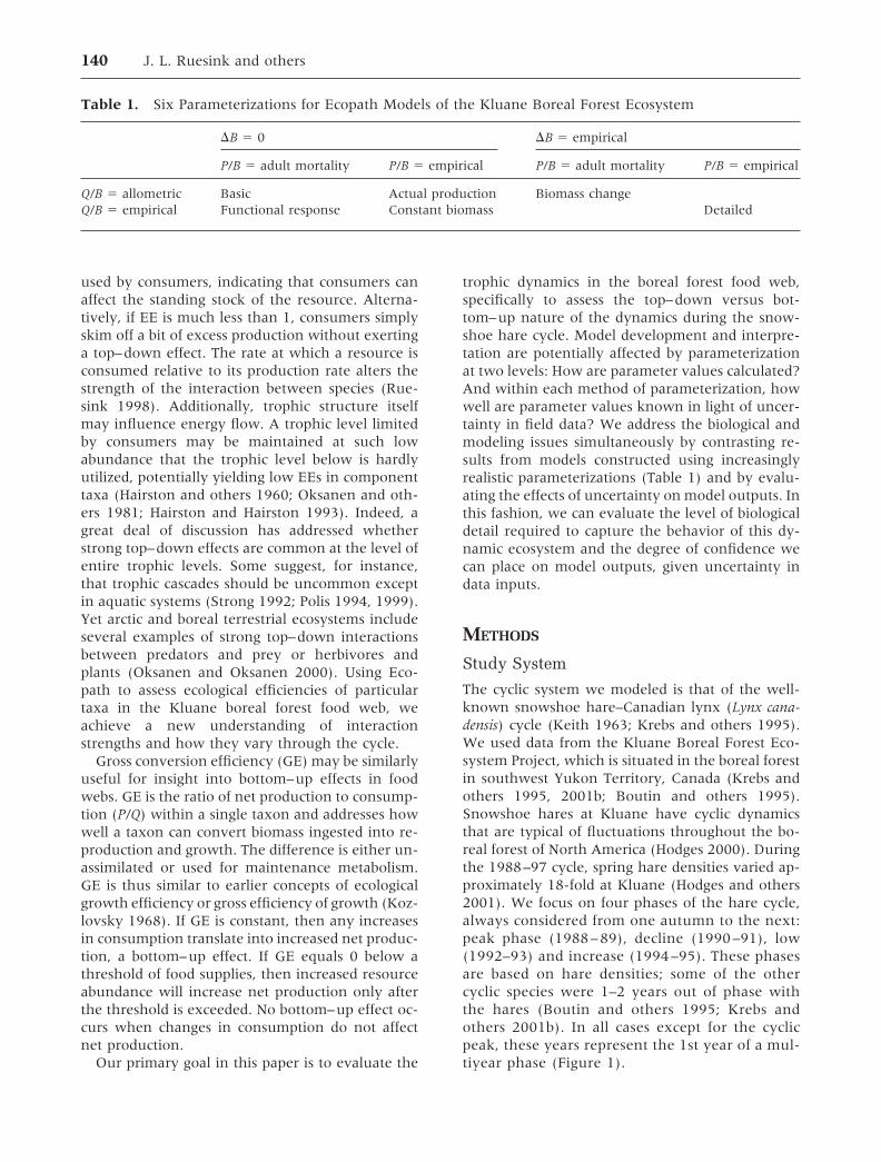
Table 1. Six Parameterizations for Ecopath Models of the Kluane Boreal Forest Ecosystem

�B � 0 �B � empirical

P/B � adult mortality P/B � empirical P/B � adult mortality P/B � empirical

Q/B � allometric Basic Actual production Biomass changeQ/B � empirical Functional response Constant biomass Detailed

140 J. L. Ruesink and others

The Kluane Project research was conducted inthe boreal forest of the Shakwak Trench (60°57�N,138°12�W), a broad glacial valley that runs eastfrom the southern end of Kluane Lake, Yukon,Canada (Figure 1). To the north and south are themountains of the Ruby and Kluane Ranges, respec-tively, while the valley itself averages 900 m abovesea level. The dominant forest tree is white spruce(Picea glauca) with patches of balsam poplar (Populusbalsamifera) and aspen (P. tremuloides) and a 0.5–2-m–tall shrub layer of birch (Betula glandulosa), wil-low (Salix spp.), and soapberry (Shepherdia canaden-sis).

Figure 1 depicts the trophic relationships amongthe most common vertebrate taxa in the Kluanefood web, which we used for the models in thispaper. A more detailed food web is given in Krebsand others (2001b). We modeled the vertebrates insome detail, but we did not explicitly model plantsor insects. We also ignored a number of small pred-ators (mustelids, foxes) and large mammals (moose,grizzly bear, wolves) that are relatively uncommonand were unstudied at Kluane. From 1988 to 1997,

experimental manipulations (fertilization, herbi-vore exclusion, food addition, predator exclusion)were conducted to evaluate the interactions of thedifferent trophic levels (Krebs and others 1995,2001b; Turkington and others 1998; Sinclair andothers 2000). In this paper, however, we use datacollected from control areas because we wish toaddress the dynamics of the unmanipulated system(see Ruesink and Hodges 2001 for Ecopath analysesof treatment effects). Whenever possible, we usedpublished demographic and trophic informationfrom the Kluane boreal forest ecosystem. We alsoused data from other boreal research papers or fromthe unpublished data of individual researchers atKluane as needed to supplement the published Klu-ane material.

Our models addressed food web dynamics for theKluane ecosystem as a whole, although particularspecies were studied at different locations withinthe Shakwak Trench. For prey species, densitieswere sampled from sites throughout the valley(Folkard and Smith 1995; Karels and others 2000;Martin and others 2001; Boonstra and others

Figure 1. Study site, foodweb, and conspicuous cy-clic dynamics in the Klu-ane boreal forest ecosys-tem. Many small birds areinsectivores, but we con-nected this taxon directlyto primary producers be-cause we were uncon-cerned with the details oflower trophic level dy-namics. Boxes superim-posed on the time seriesof hare densities showperiods explored with an-nual models.


2001a, 2001b; Hodges and others 2001), and weaveraged values from the different sites. Samplingsites ranged in area from 2.8 ha (mice and voles) to60 ha (hares and grouse). For raptors, densitieswere assessed in a 100 km2 intensive study area,and these densities were extrapolated to the entirearea (Doyle and Smith 1994, 2001; Rohner 1996;Rohner and others 2001). For the mammalianpredators, density estimates were made on a valley-wide basis—that is, 400 km2 (O’Donoghue and oth-ers 1997, 2001).

Ecopath Modeling Framework

We constructed mass-balance models of the Klu-ane food web using Ecopath. Ecopath is based onthe mass-balance models of Polovina (1984) andis a Windows-based software program developedat the International Centre for Living AquaticResources Management (www.ecopath.org),(Christensen and Pauly 1992, 1993). We param-eterized six separate Ecopath models for each ofthe four phases of the cycle (Table 1). Basic mod-els were modeled with equilibrial assumptions:no biomass change (�B equals 0), production(P/B) equivalent to adult mortality, and con-sumption (Q/B) based on allometric energy re-quirements. This parameterization method mostclosely approximates the common strategy usedin aquatic Ecopath models (Okey and Pauly1998). We created five other model types—threemodels relaxing one assumption each, one relax-ing two, and one model relaxing all three as-sumptions simultaneously. In biomass changemodels, we explicitly modeled the observedchanges in biomass (�B) of cyclic species. To relaxthe assumption of equilibrial production equalingadult mortality, we constructed actual productionmodels for which P/B was based on observedreproduction and growth. In functional responsemodels, we based Q/B on the empirically observedkill rate data of mammalian predators rather thanon allometric requirements. Constant biomassmodels included actual production and predatorfunctional responses. Finally, we constructed de-tailed models that incorporate all three of theseelaborations on the basic models. Using differentparameterizations allows us to ask questions suchas: Do functional responses of predators contrib-ute to hare population declines? (basic versusfunctional response); What proportion of net pro-duction is ingested (or at least killed) by highertrophic levels? (constant biomass); and What isthe role of variable production in driving cyclicdensity changes? (basic versus actual produc-

tion). The details of how we extracted Ecopathparameters from population-level data follow.

Biomass

For vertebrates, we had estimates of density andindividual body mass; their products provide esti-mates of biomass per area. Snowshoe hares andground squirrels were modeled with �B not equalto 0 because individual biomass and population sizevaried over time (Karels and others 2000; Hodgesand others 2001). Cyclic mammalian and avianpredators were modeled with �B not equal to 0because population sizes varied (Doyle and Smith1994, 2001; Rohner 1996; O’Donoghue and others1997; Rohner and others 2001). For hares andground squirrels, we used both fall and spring pop-ulation estimates, and we incorporated the varia-tion in body mass estimates that occurred duringthe cycle. Ground squirrels were trapped using oneregime prior to 1991 and another thereafter; weapply spring 1991 densities to previous years be-cause of the noncomparability of the trapping esti-mates from the two periods (T. Karels personalcommunication). For all other taxa, we modeledbody mass as constant through time because thenatural variation was not cyclic and the variationwas small (Krebs and Wingate 1985; Boonstra andothers 2001b; Martin and others 2001). Red squir-rel densities remained fairly constant from year toyear, but fall densities always exceeded spring den-sities, so we calculated an average fall and an aver-age spring density using data from all years (S.Boutin and others unpublished; Boonstra and oth-ers 2001a).

For lynx and coyotes, densities were estimatedover winter (O’Donoghue and others 1997). Rap-tors (great-horned owls, goshawks) were surveyedin spring (F. I. Doyle unpublished; Doyle and Smith2001; Rohner and others 2001). For all remainingvertebrate taxa (grouse, small mammals, smallbirds) we calculated average densities based on allavailable density estimates from fall 1988 to spring1996 inclusive (Folkard and Smith 1995; Boonstraand others unpublished 2001b; Martin and others2001). The densities of these taxa either had smallcoefficients of variation through time, and/or thefluctuations in their densities varied randomly withrespect to the hare population cycle. Eight species ofsmall birds contributed to that taxon (Folkard andSmith 1995). Their densities, weighted by body size,were increased 10% to account for other, rarelydetected species. The small mammal taxon com-bined values for Microtus and Clethrionomys spp.(Boonstra and others 2001b).


Consumption per Biomass (Q/B)

We used the allometric relationships between bodymass and consumption rates derived by Nagy(1987) to estimate the daily energy needs of thevarious taxa. These relationships were calculatedindependently for birds, mammalian herbivores,and mammalian predators. These energy estimateswere derived from field data and represent averageenergy needs of active animals. We calculated en-ergy needs as kcal kg–1 y–1. The biomass necessaryto meet these energy needs depends on the energycontent of the food and the efficiency of energyassimilation by the consumer. We assumed an as-similation efficiency of 80% (Parks 1982). We as-sumed the energy content of plants to be 1 kcal/gand of animals to be 1.75 kcal/g fresh weight (FW)(Parks 1982). This estimate of 1.75 kcal/g for ani-mals has been empirically confirmed for snowshoehares. Captive coyotes obtained 1.4 kcal/g FW ofmetabolizable energy from snowshoe hares(Litvaitis and Mautz 1980), which is equivalent to80% of 1.75 kcal/g. To account for migration andhibernation, we multiplied feeding rates of groundsquirrels and migratory avian predators and song-birds by one-third because these species are activeat Kluane for only 4 months of the year.

These allometric estimates of consumptionmatched independent field data (Pease and others1979; Hodges 1998) and expert opinions on feedingrates of hares and avian predators at Kluane (K.Hodges unpublished; F. I. Doyle personal commu-nication). Lynx and coyotes, however, killed haresin excess of their allometric estimate during thecyclic peak, but they killed hares at lower ratesduring the low phase (O’Donoghue and others1998b). Thus, for mammalian predators we calcu-lated separate feeding rates for each phase of thecycle using direct estimates of annual predationrates on hares, weighted by the proportion of haresin the biomass of the diet (O’Donoghue and others1998a, 1998b).

Diet Composition

The diets of lynx and coyotes were estimated fromthe analysis of prey remains in scats (O’Donoghueand others 1998b). We weighted winter scats bytwo-thirds and summer scats by one-third to relatethese diets to the seasons at Kluane. The diets ofgoshawks, Harlan’s hawks, and northern harrierswere estimated from prey remains occurring atnests in the summer (Doyle and Smith 2001). Weassumed that the adults provisioned young withfood similar to their own diets. Diets of great-horned owls were estimated from pellet remains

and prey remains at nests (Rohner 1994; Rohnerand others 2001). Most of the owl diet data wereobtained from summer estimates; we weightedboth summer and winter as half the diet for owls toreduce the contribution of limited winter data. Dur-ing winter, about 90% of their diet consists of hares(Rohner 1996), and we assumed the remainder washalf small mammal and half red squirrel. Prey re-mains indicate the number of individuals killed; toconvert to biomass, we multiplied individuals bythe average body mass of each prey type. We usedmasses of 0.1 and 0.7 kg for leverets (less than 30days old) and juvenile hares (less than 6 monthsold), respectively.

Many snowshoe hare leverets were killed by redsquirrels and ground squirrels (O’Donoghue 1994;Stefan 1998; Hodges and others 2001). To calculatethe proportion of each squirrel species’ diet com-posed of leverets, we calculated kg hares consumedper kg squirrel per year:

qLp �L � �1–SL� � mLp � bL

Bp(2)

where qLp is consumption of leverets by squirrels, Lis the number of leverets born, SL is leveret survivalrate to 30 days based on data from radiotaggedleverets, mLp is the proportion of leveret mortalitydue to squirrels, bL is the average mass of a singleleveret (0.1 kg), and Bp is total squirrel biomass.Snowshoe hare production and mortality parame-ters were taken from Stefan (1998), O’Donoghue(1994) and O’Donoghue and Krebs (1992); squirrelbiomass estimates were derived from populationestimates as shown above. We calculated squirrelconsumption of leverets separately for groundsquirrels and red squirrels. For each species, wethen determined what proportion of their total (al-lometric) consumption consisted of hares. In fact,this calculation may overestimate the contributionof hares to squirrel diet, if portions (that is, morethan 20% unassimilated) of carcasses remain un-consumed.

Production per Biomass (P/B)

For three models (basic, biomass change, functionalresponse), we used the common parameterizationtechnique of assuming that production per biomass(P/B) equals the adult mortality rate. We had esti-mates of mortality for most species (Table 2). Foractual production, constant biomass, and detailedmodels, we calculated P/B using reproduction,growth, and recruitment data. Unlike most Ecopathmodels, which use annual production divided byaverage annual biomass, we used initial fall biomass


for our denominator so that we could explicitlyaddress biomass change during the year. Similarly,our estimates of production were based on animalsthat were present in the spring. If separate fall andspring estimates were not available, as was the casefor most predators, breeding densities were as-sumed to equal fall densities.

For both raptors and mammalian predators, wecalculated production as the recruitment (R) ofyoung into the adult population (with units of in-dividuals/individual/y or kg/kg/y). This calculationdoes not incorporate the “production” of growingoffspring that died before adulthood, because wehave no data for these individuals. In terms of pa-rameterization, therefore, R is less than or equal toactual production. For raptors,

R � r � f � n (3)

and for lynx,

R � r � � A � fa � na � sa � Y � fy � ny � sy� (4)

where r is the proportion of adult females, f is theproportion of females breeding, n is litter size oryoung fledged, and s is survival until maturity. Forlynx, yearling females differed from adult femalesin their reproductive parameters (Slough and Mo-wat 1996). We therefore calculated reproductionfor each group separately, with A and Y represent-ing the proportion of females in each age class andsubscripts denoting age-specific parameters. We as-sumed that raptors fledged at adult mass, so therewas no need to include a survival term. We wereunable to locate any information on coyote repro-duction in the boreal forest, so we modeled coyote

production as identical to lynx production: Thetemporal patterns in hunting group sizes of lynxand coyotes (an index of reproduction) at Kluanewere similar (O’Donoghue and others 1997). Wecalculated production by small mammals (6.6 y�1)and grouse (2.2 y�1) using similar equations. Forsmall birds, we set P/B equal to 2 y�1 becausefledging rates should at least equal those of largeravian species. Also, fledging rates for warblers inHubbard Brook deciduous forest had median valuesof 3 or 4 per pair (Rodenhouse and Holmes 1992),close to P/B � 2 y�1.

For the remaining taxa, data were available onthe growth rates and survival of the young, thusallowing us to include the biomass of young that didnot reach adulthood in our estimates of production.For ground squirrels and red squirrels, production(P) was calculated from emergence from the nest(when offspring first become vulnerable to preda-tion) to adulthood, using the following equation:

P � d � r � f � n � � b � �t�0

tj

g � emt� (5)

where d is the breeding density, r is the proportionof females in the breeding population, f is the pro-portion of females breeding, n is litter size, b isindividual offspring mass at emergence, g is thedaily growth rate of young, m is the daily exponen-tial mortality rate (m less than 0), and t is the timeat which animals leave the juvenile stage, calcu-lated from the difference between emergence andadult weights divided by growth rate. To obtainproduction per biomass, this production was di-

Table 2. Annual Survival Calculations Used for Production/Biomass values (P/B � adult mortality �1–survival) in Basic, Functional Response, and Biomass Change Models

Adult SurvivalInterval

YearsAvailable

AnnualSurvivalCalculation

Survival Values forFour Phases of Cycle

Hares Annual Apr–Mar (sa) 1988–96 (sa � sa�1)/2 0.25, 0.07, 0.10, 0.25Ground squirrels 28-d active season (s28) 1990–96 exp(4 ln(s28)) (so) 0.32a, 0.33, 0.15, 0.39

Overwinter (so)Red squirrels Mar–Aug (ss) 1988–96 (ss) (so) 0.81, 0.58, 0.62, 0.50

Sept–Feb (so)Lynx 30-wk overwinter 1988–96 Use directlyc 0.75, 0.69, 0.06, 1.0Great-horned owl Annual fall–fall 1989–92 Use directly 0.93, 0.96, 0.60, 0.60b

Four phases correspond to hare peak (1988–89), decline (1990–91), low (1992–93), and increase (1994–95).aGround squirrel survival at the peak was unavailable for 1988–89, so average values from the other three model years were used.bGreat-horned owl survival was available only for 1990–91 (0.97) and 1991–92 (0.60). We took these as representative of times when hares were common vs rare.cOverestimates survival.


vided by fall biomass. For ground squirrels, we usedyear-specific data for all parameters except size ofemerging young (for which only 1993 data wereavailable) and growth rate (which appears to re-main constant) (T. Karels personal communica-tion). We used year-specific birth, growth, and sur-vival data for red squirrels, although populationdensities were kept constant because interannualvariation in density was low.

For hares, mortality rates of leverets differed fromthose of juveniles, which required that we distin-guish the production accruing from each stage. Spe-cifically:

P � d � r � �L�1

4

fL � nL � �bL ��t�0

t1

gL � emL�t1 ��t�t1

t2

gj � emj �t2�(6)

Variables are the same as in the production equa-tion for squirrels, with L referring to the littergroup—that is, bL, gL, and mL (less than 0) refer tothe birth weight, growth rate, and daily mortalityrate per litter group. Juvenile parameters forgrowth (gj) and daily mortality rate (mj less than 0)were assumed constant for all litter groups. We hadjuvenile survival data only for the increase year of1995–96 (Gillis 1998), so these values were appliedto all years, whereas we used year-specific leveretparameters (O’Donoghue and Krebs 1992;O’Donoghue 1994; Stefan 1998). The time units t1and t2 represent days to the end of the leveret andjuvenile phases, respectively, and were calculatedbased on the length of time it would take for anindividual to grow to the next phase (that is, forleverets to reach 0.5 kg and for juveniles to reachadult weight), given known initial biomass andgrowth rate. The growth rate of leverets differedslightly among litter groups 1 and 2, and growthrates of leverets in litters 3 and 4 were assumed tobe intermediate (O’Donoghue and Krebs 1992).

Although the vertebrate food web is fueled byprimary productivity of plants, we did not modelplant production explicitly. In a separate paper, wehave shown that sufficient plant biomass exists atKluane to support energetic requirements of herbi-vores, even at the peak of the hare cycle (Ruesinkand Hodges 2001; Sinclair and others 2001). Ourcalculations of available plant biomass excludeinedible tissues such as tree trunks but do nototherwise address issues of food quality. If plantnutritional quality were low, herbivores could ex-perience food limitation despite high plant biomass.For example, dietary protein content affects harebody mass and starvation rates (Sinclair and others

1982; Rodgers and Sinclair 1997). The trophic ma-nipulations at Kluane have also shown that foodsupply and predation pressure interact in their ef-fects on snowshoe hare population dynamics, pos-sibly resulting from foraging changes by hares inresponse to predation risk (Krebs and others 1995,2001a).

Modeling Uncertainty in SnowshoeHare Parameters

Ecopath was used to generate ecotrophic efficien-cies (EE) and gross conversion efficiencies (GE) forvertebrates in the Kluane food web (Figure 1) forfour phases of the cycle and for six of eight possiblemethods of parameterization (Table 1). In all cases,we parameterized Ecopath using mean values. Con-sequently, the models provide no indication of thecertainty of the estimates of energy flow throughthe Kluane food web. For snowshoe hares only, wecarried out separate calculations for EE that incor-porated variation in parameter values. Specifically,we calculated EE repeatedly in a Monte Carlo sim-ulation in an Excel spreadsheet (Excel 2000; Mi-crosoft, Redmond, WA, USA). We based simula-tions on Eqs. (1) and (6), assuming that �B equals0, which is equivalent to the constant biomass Eco-path model. For each simulation run, we drew val-ues for each parameter randomly from its probabil-ity density function. Mean values, variation, anddistribution type for each parameter are provided inTable 3.

Densities, feeding rates, and the diet compositionof predators at Kluane are point estimates withoutestimates of uncertainty. Therefore, de facto, ourexplorations of uncertainty in snowshoe hare EEderive exclusively from variation in parameters as-sociated with hare production. Variation in hare EEwould probably be larger if consumption parame-ters derived from predation data also had associatederror estimates. For example, Nagy’s (1987) esti-mates of field metabolic rates have confidence lim-its of �58% to �138%, which could increase esti-mates of losses to predators, and therefore EE, overtwofold.

In translating parameter values for hare produc-tion into Monte Carlo simulations, three problemsarise. First, two ways of estimating variation in haredensity are possible. Each grid had variation asso-ciated with its mean value based on mark-recapturetechniques (Krebs 1999; C. J. Krebs and othersunpublished) and, because hares were trapped onup to three control sites, variation existed in themean density among sites (Hodges and others2001). We used the latter estimate of mean (SD)hare density because we were more interested in


the natural variation in hare densities that occurs inthe boreal forest than in the variation accruing frommethodological problems. Furthermore, the varia-tion among grids was larger than the variationwithin grids.

Second, no data for hare reproduction were col-lected during the low phase in 1993. To model harereproduction during the cyclic low phase, we aver-aged values from 1992 and 1994 and used the max-imum standard deviation (SD). Survival of radio-tagged leverets was measured as 0 in 1992, but weknow this value to be an underestimate of reproduc-tion because some juvenile hares were captured in fall1992. We parameterized the low-phase model by us-ing both the mean and SD for leveret survival in 1994divided by two, which probably yields an underesti-mate of true leveret survival in 1993.

Third, uncertainty in some parameters was suffi-ciently large that the probability density functionencompassed unreasonable values. For instance,some randomly chosen values of peak hare densi-ties were less than the average low density, andsome survival values were less than 0% or morethan 100%. When randomly chosen values for thesimulations fell outside the realm of possibility, we

chose new values. This strategy effectively reducedvariation in parameter values and also led to direc-tional change in the mean values of some parame-ters. For instance, during the peak, leveret survivalwas less than 0 for 20% of randomly chosen valuesfor litters 2 and 3 and had to be reselected. Never-theless, through these Monte Carlo simulations, wedetermined whether EE of hares at different stagesof the cycle could be differentiated once uncertaintywas incorporated.

RESULTS

Insight into food web dynamics emerges fromcomparisons of EE and GE as the models becomemore realistic and in reference to different cyclicphases. All models of the Kluane boreal forestfood web were based on the same trophic struc-ture (Figure 1), yet they yielded different esti-mates of energy flow and conversion efficiencies(Figures 2–5). For all parameterizations, energyflow varied through the cycle. For the six herbi-vore taxa, EE varied by more than 50% throughthe cycle (Figure 2). EEs of carnivores varied onlywhen we modeled annual changes in biomass,

Table 3. Parameter Values for Monte Carlo Simulations of Snowshoe Hare Ecotrophic Efficiency fromO’Donoghue (1994) and Stefan (1998)

Peak 1988–89 Decline 1990–91 Low 1992–93 Increase 1994–95

Fall density (ha�1) 2.28 (0) [1] 1.62 (0) [1] 0.13 (0.005) [3] 0.53 (0.15) [3]Spring density (ha�1) 0.74 (0.54) [3] 0.87 (0.09) [2] 0.08 (0.02) [3] 0.18 (0.10) [3]Adult individual biomass (kg) 1.51 (0.17) [70] 1.46 (0.14) [83] 1.33 (0.15) [11] 1.41 (0.10) [25]Proportion female 0.42 [72] 0.39 [87] 0.50 [12] 0.37 [28]Proportion reproductive

Litter 1 0.94 [32] 1.0 [7] 0.89 [23]a 1.0 [17]Litter 2 0.97 [31] 0.85 [13] 1.0 [17]a 1.0 [17]Litter 3 0.82 [34] 0 [13] 0.5 [8]a 1.0 [12]

Litter sizeLitter 1 3.6 (0.9) [8] 3.3 (1.1) [7] 3.2 (1.0) [17]a 3.0 (1.2) [6]Litter 2 6.0 (1.4) [13] 4.2 (2.0) [11] 5.2 (2.1) [12]a 6.9 (1.5) [9]Litter 3 4.4 (1.1) [7] — 3.2 (0.5) [11]a 5.6 (1.7) [8]

Birth weight (g)Litter 1 52.7 (7.1) [7] 46.2 (4.5) [7] 51.8 (9.2) [13]a 59.9 (8.8) [6]Litter 2 54.3 (11.4) [12] 53.2 (10.3) [11] 54.8 (4.8) [10]a 57.9 (7.5) [9]Litter 3 69.3 (12.2) [7] — 64.5 (4.7) [10]a 70.3 (4.8) [7]

Leveret 30-d survival, transformedb

Litter 1 1.02 (0.52) [12] 0.76 (0.49) [17] 0.52 (0.68) [36]a 1.0 (0.52) [19]Litter 2 0.49 (0.58) [23] 0 (0) [21] 0.45 (0.35) [50]a 0.90 (0.49) [49]Litter 3 0.44 (0.53) [11] — 0.61 (0.27) [50]a 0.89 (0.50) [31]

Values for numbers and biomasses are means (SD) [sample size]. Proportions are assumed to be binomially distributed; mean values [and sample sizes] are given.aAll values are interpolated from data collected in spring 1992 and 1994 because reproductive data were not recorded in 1993.bLeveret survival was available as Kaplan-Meier estimates (mean and SE). Prior to simulations, these values were arcsine-square root–transformed to improve normality.Transforming the SEs generated asymmetric variation around the transformed mean, but we assumed the variation to be normal and of intermediate magnitude. Randomvalues were chosen from this new distribution, back-transformed to survival, and finally ln-transformed to provide daily mortality rates for use in Eqs. (1) and (6).


because no other fates of production (for exam-ple, intraguild predation or trapping) were in-cluded. EEs varied 100% through the cycle forlynx, coyotes, great-horned owls and goshawksin the detailed and biomass change models, ex-ceeding 0 during population increases.

The parts of the food web showing most variationin EE and GE do so for the following two reasons:(a) because production varies (as P/B increases, EEdeclines and GE increases), and (b) because con-sumption varies (as consumption increases, the GEof that taxon declines and the EEs of lower trophiclevels increase). Most variation in energy flow is

therefore due to within-species variation in net pro-duction and consumption; but in some cases, par-ticularly for herbivores, EE varies due to consump-tion rates of predators (a between-species effect).Table 4 shows the range of variation in net produc-tion and consumption among species across thefour phases and hence illustrates the diversity ofvalues feeding into the Ecopath models for eachphase. For five taxa (small mammals, grouse, smallbirds, Harlan’s hawks, northern harriers), welacked sufficient data to evaluate cyclic variationfully, so we devote little consideration to theamong-phase results for these taxa.

Figure 2. Ecotrophic effi-ciency (EE) throughout thecycle for (A) snowshoehares, (B) ground squirrels,(C) red squirrels, and (D)other herbivores. Graphs(A–C) depict EE calculatedfrom six different param-eterizations of Ecopath. Forother herbivores, EE wasaffected only by feedingrates of mammalian preda-tors (allometric or func-tional response) and variedby up to 55% among pa-rameterizations. Note thedifferent y-axis scales.


Ecotrophic Efficiency

Ecotrophic efficiencies were less than 1 in all mod-els for all herbivores except hares and ground squir-rels (Figure 2). When EE is greater than 1, modelsare unbalanced because there is not enough pro-duction to account for all the fates of a species’biomass. Hares had EE greater than 1 in three gen-eral cases—for the actual production and constantbiomass models of the decline (actual productionwas less than mortality and the biomass decline wasnot incorporated); for the biomass change model ofthe increase (P/B was low because mortality waslow but biomass increase was incorporated); and forall models during the cyclic low. Ground squirrelshad an EE greater than 1 only for the increasebiomass change model, suggesting that P/B equal tomortality could not account for observed popula-tion increases. For small mammals, grouse, andsmall birds, EEs were low but variable; this varia-tion was due to parameterizations of predators, be-cause their own production was assumed to beconstant through the cycle and across model types.

Snowshoe Hares. The detailed and constant bio-mass models produced EE approximately equal to 1for snowshoe hares during the decline and low, justas would be expected if predators consume standingstock in addition to production (Figure 2A). In con-trast, snowshoe hare declines would not have beenexpected based on basic models (EE equals 0.55),and both basic and biomass change models werehighly unbalanced (EE greater than 1) during the

low. Changing the models to incorporate actualproduction or predator functional responsesbrought the models closer to observed dynamics,essentially raising consumption relative to produc-tion of hares during the decline, and lowering thatratio during the low phase. Increases in hare den-sities were only likely when P/B equals actual pro-duction rather than adult mortality (detailed versusbiomass change models during the increase phase).The large distinction in model results related tousing actual production versus adult mortality forP/B of hares occurred because mortality and repro-duction tended to be inversely correlated.

The results from constant biomass models high-light the consumption of a species relative to itsproduction and therefore indicate trophic links forwhich top–down impacts are likely to occur. Snow-shoe hares had their lowest EEs—0.16 and 0.36—

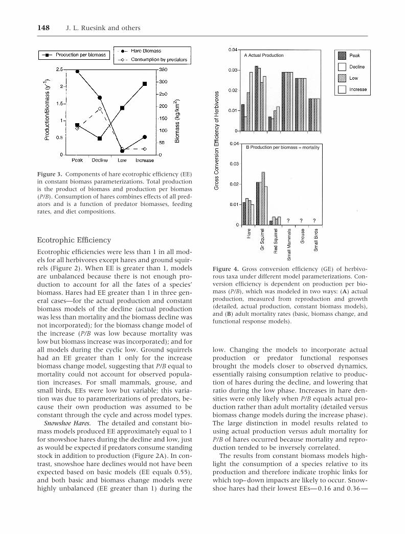
Figure 3. Components of hare ecotrophic efficiency (EE)in constant biomass parameterizations. Total productionis the product of biomass and production per biomass(P/B). Consumption of hares combines effects of all pred-ators and is a function of predator biomasses, feedingrates, and diet compositions.

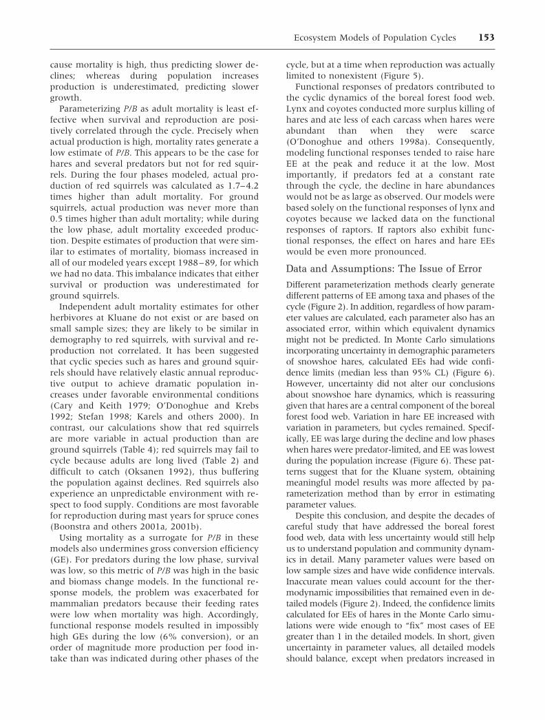
Figure 4. Gross conversion efficiency (GE) of herbivo-rous taxa under different model parameterizations. Con-version efficiency is dependent on production per bio-mass (P/B), which was modeled in two ways: (A) actualproduction, measured from reproduction and growth(detailed, actual production, constant biomass models),and (B) adult mortality rates (basic, biomass change, andfunctional response models).


during the increase and peak phases, respectively,and had much higher EEs—1.67 and 1.10—duringthe decline and low phases (Figure 2A). The 10-folddifference in hare EEs, and EE greater than 1 in twocyclic phases, indicate a dramatic variation in thestrength of the top–down effect of predators onhares. During periods of biomass decline, all of thesnowshoe hare production and some of the stand-ing stock were consumed by predators. As haresincreased, predators still consumed more of the pro-duction than they did for the other herbivoroustaxa, but hare production exceeded predator con-sumption.

Because of the central role of hares in the borealforest food web (Ruesink and Hodges 2001), weexplored EE in more depth by examining the cyclicchanges in parameters contributing to EE. In Figure3, we present the parameters that compose EE—standing biomass of hares, production per biomass,and biomass of hares consumed. These factors show

whether shifts in population trajectories can be at-tributed to how many hares are present, their percapita reproductive rates, or predation pressure. Inthe decline phase, two factors changed relative tothe previous phase—predator numbers increased(as indicated by consumption of hares) and hareP/B declined. The decline phase of the cycle appearsto be caused by a combination of top–down andbottom–up changes, with high consumption ofhares not compensated for by low per capita repro-duction. Similarly, both production and predationinteract to allow the shift from low to increasinghare densities. The low and increase phases wereequivalent in terms of consumption of hares, buthares had slightly higher biomass and per capitaproduction during the shift from low phase to in-crease, which was sufficient for them to “escape”control by predators.

Other Herbivores. Relative to hares, other herbi-vores had lower EEs in constant biomass models,

Figure 5. Gross conver-sion efficiency (GE) ofpredator taxa calculatedfrom six different param-eterizations of Ecopath.Conversion efficiency isdependent on productionper biomass (P/B), whichwas modeled from repro-duction and growth dataor as equivalent to adultmortality, and consump-tion per biomass (Q/B),which was modeled fromfield data or allometri-cally. Basic and biomasschange models yield thesame results because bothare based on P/B equal tomortality and allometricQ/B; similarly, detailedand constant biomassmodels yield the sameresults because both arebased on P/B equal to ac-tual production and Q/Bequal to observed feedingrate of mammalian preda-tors. (A) Detailed andconstant biomass models,(B) basic and biomasschange models, (C) func-tional response model,(D) actual productionmodel.


indicating that they were less likely to be predator-limited. Of course, several predators not included inthese models (mustelids, foxes, other raptors)would undoubtedly raise EEs of these alternativeprey. Even in this restricted food web, however,there was substantial variation in EE for herbivoresother than hares. For red squirrels, grouse, andsmall birds, EEs were highest when predators wereabundant during the peak and decline phases. Forground squirrels, however, EE was highest whenpredators were rare, probably due to a combinationof relatively low ground squirrel biomass (thereforelittle production) and larger proportions of groundsquirrels in the diets of predators (ground squirrelsas a percentage of diet compositions rose by up to20%) (Doyle and Smith 2001).

For red squirrels and ground squirrels, basic mod-els yielded low EEs through the cyclic phases, withEEs ranging from 0.06 to 0.30 and 0.04 to 0.15 forthe two species (Figures 2B and C). Ground squir-rels have generally been shown to undergo popu-lation cycles in concert with hares (Boutin andothers 1995), but in the years we modeled, groundsquirrels consistently increased (Boonstra and oth-ers 2001a). Thus, incorporating biomass change ledto much higher EEs of 0.58, 0.74, and 1.24 duringthe decline, low, and increase phases, respectively;but detailed models all had EE less than 1, meaningthat these increases were possible given actual pro-duction and predation (Figure 2B). For both squir-rel species, P/B was generally higher when calcu-lated from actual production than from adult

mortality; consequently, EEs in actual productionmodels were lower than in basic models. Becausered squirrels were given constant biomass in allmodels, basic and biomass change EEs were identi-cal, as were detailed and constant biomass EEs (Fig-ure 2C). Modeling the functional response of pred-ators led to a greatly increased EE for red squirrelsduring the peak phase (from 0.30 to 0.46), butcaused little change during the other phases. Mod-eling the functional response had a proportionallysmaller effect on the EEs of ground squirrels (from0.037 to 0.047) because feeding rate changes inmammalian predators were diluted by constant (al-lometric) feeding by avian predators

Predators. The EEs for predators were always 0unless biomass change was incorporated (biomasschange and detailed models), because we includedno fates for predator production other than biomassaccumulation. Harlan’s hawks and northern harri-ers always had EE equal to 0 because their popula-tions were assumed invariant. For other predators,EE was greater than 0 in models and years whenbiomass increased. In detailed models, productionkept pace with biomass increases for lynx, coyotes,and great-horned owls during the peak phase, butdid not match empirical population increases ofgoshawks at the peak and low. Furthermore, lynxand coyotes increased in density in 1994–95 (hareincrease phase) when no predator reproductionwas observed (O’Donoghue and others 1997); theirEEs for detailed and biomass change models wereeffectively infinite. The biomass change models

Table 4. Summary of How Parameters Varied among Phases of the Cycle, Showing Range of FieldMeasurements for 4 Modeled Years of Detailed Models

Biomass(kg/km2)

Production/Biomass(P/B) (y�1)

Consumption/Biomass(Q/B) (y�1)

Annual BiomassChange (�B)(kg/km2)

Snowshoe hares 17–343 0.48–2.10 71 �78–�76Ground squirrels 45–107 0.78–1.02 32a �22–�56b

Red squirrels 61 0.72–1.43 115 0Lynx 0.24–1.77 0–2.06 25–67 –0.94–�1.00Coyotes 0.20–0.99 0–2.06c 15–123 –0.42–�0.26Great-horned owl 0.31–1.16 0–1.05 39 –0.48–�0.17Goshawk 0.02–0.06 0.5–1.5 42 –0.02–�0.06Harlan’s hawk 0.22 0.3–0.8 14a 0Northern harrier 0.04 0.9–2.0 17a 0

Demographic measurements for grouse, small mammals, and small birds also varied among years, but this variation was not incorporated because its magnitude was smallor uncertain. In most cases, parameters modeled with cyclic variation were also modeled differently among parameterization methods. Exceptions, which were consistent amongall parameterizations, were starting biomasses of all taxa and P/B values of goshawks, Harlan’s hawks, and northern harriers. Diet composition varied through the cycle forall predators but was kept constant among different parameterization methods.aQ/B reduced to one-third for migratory and hibernating species (also includes small birds).bGround squirrel changes in biomass were modeled only after 1991.cCoyote P/B values were assumed to equal lynx values.


generated EE greater than 1 for all four cyclic pred-ators during the peak. These high EEs occurredbecause production was modeled after adult mor-tality—which was lower than actual production—while the biomass increased.

Gross Conversion Efficiency of Herbivores

Only two patterns for herbivore GE emerged fromthe six methods of parameterizing Ecopath models(Figure 4). This result occurred because the con-sumption component of GE was always based onallometry, while the production component forsnowshoe hares, red squirrels, and ground squirrelstook on one of two parameterizations—actual pro-duction (actual production, constant biomass, anddetailed models) or adult mortality (basic, biomasschange, and functional response models). VariableGEs (0.007–0.029) based on actual production byhares reflect substantial variation in reproductionthrough the cycle (because consumption was as-sumed constant). For red squirrels and groundsquirrels, reproductive output was much more con-sistent over time, thus resulting in fairly steady GEs(0.006–0.012 and 0.024–0.032, respectively). Us-ing the second parameterization method, of P/Bequal to mortality, GEs were lowered for snowshoehares, ground squirrels, and red squirrels. Addition-ally, hare GEs were much more consistent with thisparameterization, ranging only between 0.010 and0.013. There were only single estimates of P/B forsmall mammals, grouse, and small birds, and theseestimates were considered invariant across cyclicphases, so these three taxa had single values for GEof 0.029, 0.026, and 0.016, respectively. Small birdshad particularly high GE because we incorporatedjust 3 months of summer feeding.

Gross Conversion Efficiency of Predators

For mammalian predators, we were able to param-eterize both production and consumption from fieldestimates. We therefore generated four estimates ofGE from the six models. Basic and biomass changemodels were the same with respect to GE, as weredetailed and constant biomass models. The basicand biomass change models yielded the highest GEsduring the low phase (0.026 for lynx, 0.027 forcoyote) (Figure 5), reflecting high mortality (equalto P/B). In other phases, GEs were less than 0.009.This temporal pattern was mirrored in the func-tional response model, but because observed feed-ing rates were lower than allometric during the lowphase, GEs were higher. The actual productionmodel produced the inverse temporal pattern, withGEs of 0 during the low phase and GEs of 0.057 and

0.027 during the peak and decline phases. The de-tailed model produced relatively low GEs overall(less than 0.04), with the lowest GEs in the low andearly increase phases when little predator reproduc-tion occurred. GEs at other phases reflected killrates rather than actual consumption, and loweringassimilation to account for surplus killing wouldtend to raise GEs during phases when mammalianpredators reproduced.

For avian predators, we only had allometric esti-mates of consumption rates. P/B varied through thecycle for all species based on fledging success, butadult mortality data (and thus a second parameter-ization method) existed only for great-horned owls.Therefore, GE changed through the cycle withfledging success rates, which were generally highestwhen hares were abundant (goshawk GE equals0.036 at the peak, Harlan’s hawk GE equals 0.058 atthe low, northern harrier GE equals 0.119 at thepeak, great-horned owl GE equals 0.027 at thepeak). Values were three times too high for migra-tory species (Harlan’s hawk and northern harrier)because we included only summer consumption.As with mammalian predators, using P/B equal toadult mortality for owls reversed the cyclic patternof GE, resulting in unlikely values of 0.01 whenhares were rare and 0.001 when hares were com-mon (Figure 5).

Modeling Uncertainty in SnowshoeHare Production

The point estimates of EE calculated with Ecopathobscure substantial uncertainty in estimates of en-ergy flow (Figure 6). Based on Monte Carlo simu-lations, the 95% confidence bands around EE ofsnowshoe hares were as large as median values.Nonetheless, these simulations indicate that Eco-path successfully described cyclic differences in en-ergy flow: Both Ecopath and Monte Carlo simula-tions calculated that EE of hares differedsystematically through the cycle (Increase �Peak Low Decline). In all cases, the value of EEwe obtained from mean parameter estimates fellwithin the 95% confidence limits (CL) of the sim-ulated values. Monte Carlo simulations producedsome bias in EE. At the peak and low, the EEgenerated by Ecopath was two times higher thanthe median value from simulations. However, pop-ulation cycles still emerged. Specifically, during in-crease and peak phases, less than 10% of simula-tions produced EE greater than 1, so biomass couldincrease; whereas during the decline and low, morethan 80% of simulations would require a loss ofhare biomass in order to balance. Decline and lowphase EEs calculated in Ecopath fell outside the


95% CL of simulations for the increase and peak,and vice versa. Therefore, these phases of the cycleare marked by significantly different pictures oftop–down effects on snowshoe hares.

DISCUSSION

The Ecopath models we generated show one clearmodeling effect and two general biological patterns.Methodologically, the parameterization techniquehas large impacts on the estimates of ecotrophic andconversion efficiencies for many of the taxa. Forexample, cyclic patterns of GE were inverted be-tween functional response and actual productionmodels for predators (Figure 5). Biologically, differ-ences in the strength of top–down effects existamong species and among phases of the hare cycle,as highlighted by the variable EEs of herbivores(Figure 2). Finally, because GE is a physiologicalparameter and expected to stay relatively constant,the observed differences in productivity throughthe cycle imply strong bottom–up effects on speciessuch as hares, great-horned owls, and mammalianpredators (Figures 4 and 5).

Insights from DifferentParameterization Methods

Detailed models, which incorporated realistic dataon production, consumption, and density fluctua-tions, outperformed the models containing one or

all of the simplifying assumptions of P/B equalsmortality, no functional responses, and no biomasschange. The detailed models did better at matchingconspicuous dynamics, such as fluctuations in bio-mass and reproduction when food was abundant.Interestingly, detailed models had essentially thesame proportion of cases that violated thermody-namic principles (EE greater than 1 in five of 48cases [10%] versus 26 of 240 cases [11%] for othermodels). However, detailed models often broughtEEs closer to 1 when other parameterizations hadvalues that were very low or very high, and theygenerated GEs that were most consistent throughthe cycle (Figures 2, 4, and 5). Comparing detailedmodels to other parameterizations generates ex-plicit insight into the roles of production and con-sumption in the dynamics of this cyclic system. Ofcourse, because we use data for a single cycle at asingle location, we cannot determine how our con-clusions apply to boreal forest food webs in general.

Constant biomass models highlighted the relativevalues of actual production and consumption rates,thus giving the clearest indication of how muchproduction by a taxon is consumed. When EE wasmuch greater 1 in constant biomass models (forexample, hares during the decline phase), incorpo-rating the observed drop in hare density eliminatedthe imbalance in EE (detailed model). Conversely, ifa taxon does not increase in biomass when EE ismuch less than 1 in constant biomass models, thenit must be limited by some factor other than preda-tion from taxa in the model; small birds and smallmammals provide good examples of this pattern(Figure 2). In this context, it should be noted thatwe did not model all of the mammalian or avianspecies at Kluane. For example, weasels (althoughrelatively rare) are probably the main predator ofsmall mammals, and including weasels in Ecopathmodels would clearly lead to higher EEs for volesand mice. The constant biomass models thus revealthe extent to which predators that rely on snow-shoe hares affect other prey species in this foodweb, but these models do not exhaustively charac-terize the dynamics of all vertebrate taxa at Kluane.

It is not at all surprising that parameterizing P/Bas adult mortality would fail in this nonequilibrialfood web. An excess of production over mortality isrequired for biomass to accumulate, so of necessitymortality was lower than actual production forcases such as lynx at peak hare densities and haresduring the increase phase. Similarly, mortality mustexceed production for standing biomass to decline.Defining P/B as equal to mortality therefore leads tocycles of the wrong shape. During periods of pop-ulation decline, production is overestimated be-

Figure 6. Uncertainty in ecotrophic efficiency (EE) ofhares based on Monte Carlo simulations incorporatingvariance in parameter estimates. Monte Carlo results arepresented as median 95% CL based on 200 simulationruns. For comparison, we show the single values of EEcalculated via Ecopath for constant biomass models.


cause mortality is high, thus predicting slower de-clines; whereas during population increasesproduction is underestimated, predicting slowergrowth.

Parameterizing P/B as adult mortality is least ef-fective when survival and reproduction are posi-tively correlated through the cycle. Precisely whenactual production is high, mortality rates generate alow estimate of P/B. This appears to be the case forhares and several predators but not for red squir-rels. During the four phases modeled, actual pro-duction of red squirrels was calculated as 1.7–4.2times higher than adult mortality. For groundsquirrels, actual production was never more than0.5 times higher than adult mortality; while duringthe low phase, adult mortality exceeded produc-tion. Despite estimates of production that were sim-ilar to estimates of mortality, biomass increased inall of our modeled years except 1988–89, for whichwe had no data. This imbalance indicates that eithersurvival or production was underestimated forground squirrels.

Independent adult mortality estimates for otherherbivores at Kluane do not exist or are based onsmall sample sizes; they are likely to be similar indemography to red squirrels, with survival and re-production not correlated. It has been suggestedthat cyclic species such as hares and ground squir-rels should have relatively elastic annual reproduc-tive output to achieve dramatic population in-creases under favorable environmental conditions(Cary and Keith 1979; O’Donoghue and Krebs1992; Stefan 1998; Karels and others 2000). Incontrast, our calculations show that red squirrelsare more variable in actual production than areground squirrels (Table 4); red squirrels may fail tocycle because adults are long lived (Table 2) anddifficult to catch (Oksanen 1992), thus bufferingthe population against declines. Red squirrels alsoexperience an unpredictable environment with re-spect to food supply. Conditions are most favorablefor reproduction during mast years for spruce cones(Boonstra and others 2001a, 2001b).

Using mortality as a surrogate for P/B in thesemodels also undermines gross conversion efficiency(GE). For predators during the low phase, survivalwas low, so this metric of P/B was high in the basicand biomass change models. In the functional re-sponse models, the problem was exacerbated formammalian predators because their feeding rateswere low when mortality was high. Accordingly,functional response models resulted in impossiblyhigh GEs during the low (6% conversion), or anorder of magnitude more production per food in-take than was indicated during other phases of the

cycle, but at a time when reproduction was actuallylimited to nonexistent (Figure 5).

Functional responses of predators contributed tothe cyclic dynamics of the boreal forest food web.Lynx and coyotes conducted more surplus killing ofhares and ate less of each carcass when hares wereabundant than when they were scarce(O’Donoghue and others 1998a). Consequently,modeling functional responses tended to raise hareEE at the peak and reduce it at the low. Mostimportantly, if predators fed at a constant ratethrough the cycle, the decline in hare abundanceswould not be as large as observed. Our models werebased solely on the functional responses of lynx andcoyotes because we lacked data on the functionalresponses of raptors. If raptors also exhibit func-tional responses, the effect on hares and hare EEswould be even more pronounced.

Data and Assumptions: The Issue of Error

Different parameterization methods clearly generatedifferent patterns of EE among taxa and phases of thecycle (Figure 2). In addition, regardless of how param-eter values are calculated, each parameter also has anassociated error, within which equivalent dynamicsmight not be predicted. In Monte Carlo simulationsincorporating uncertainty in demographic parametersof snowshoe hares, calculated EEs had wide confi-dence limits (median less than 95% CL) (Figure 6).However, uncertainty did not alter our conclusionsabout snowshoe hare dynamics, which is reassuringgiven that hares are a central component of the borealforest food web. Variation in hare EE increased withvariation in parameters, but cycles remained. Specif-ically, EE was large during the decline and low phaseswhen hares were predator-limited, and EE was lowestduring the population increase (Figure 6). These pat-terns suggest that for the Kluane system, obtainingmeaningful model results was more affected by pa-rameterization method than by error in estimatingparameter values.

Despite this conclusion, and despite the decades ofcareful study that have addressed the boreal forestfood web, data with less uncertainty would still helpus to understand population and community dynam-ics in detail. Many parameter values were based onlow sample sizes and have wide confidence intervals.Inaccurate mean values could account for the ther-modynamic impossibilities that remained even in de-tailed models (Figure 2). Indeed, the confidence limitscalculated for EEs of hares in the Monte Carlo simu-lations were wide enough to “fix” most cases of EEgreater than 1 in the detailed models. In short, givenuncertainty in parameter values, all detailed modelsshould balance, except when predators increased in


density but were not observed to reproduce (implyingimmigration). In contrast, other analyses of the harecycle that incorporate uncertainty in parameter val-ues have not been able to balance production andmortality. In a stage-structured stochastic demo-graphic model using Kluane data from 1995–96, Hay-don and others (1999) found that the estimates ofsnowshoe hare fecundity and survival rates were toolow to account for the observed population increase.They speculated that survival rates may be underes-timated by current methods, perhaps because han-dling animals increases the chance that they or theiroffspring will die.

Nonequilibrial Food Webs and ChangingPredator–Prey Interactions

The nonequilibrial nature of the boreal food webcannot be summarized by a single mass-balancemodel but instead would be best encapsulated byseparate models for each year of the approximately10-year hare cycle. Based on flows of biomass (EEand GE) in the detailed models of the four cyclicphases, there is cyclic variation in the strength oftop–down and bottom–up interactions in the foodweb. Snowshoe hares showed the greatest variationin EE among herbivores: Both production and pre-dation rates fluctuated dramatically, combining toinfluence hare EE. In particular, the decline phasewas associated with high mortality due to predation(predator densities and kill rates were high) andlow per capita reproduction (Figure 3). The cause ofthis reduced reproductive rate remains unknown,but it could include a lack of high-quality food,reduced foraging to avoid predation, or physiolog-ical stress induced by high predator densities (Caryand Keith 1979; Vaughan and Keith 1981; Hik1995; Boonstra and others 1998).

It has been argued that the transition from peakdensities to declining densities occurs because of aninteraction between top–down and bottom–up fac-tors: Hare production drops and is exceeded bymortality induced by predators (Krebs and others1995). In our detailed model, P/B was relatively lowat the peak and consumption of hares was high;however, EE remained less than 1 (0.40), whichindicates the possibility of continued biomass in-crease by hares. During peak densities, hares wereso abundant that even low per capita productionresulted in high total production. Therefore, re-duced reproduction by itself was not nearly enoughto initiate the decline; high mortality rates were alsonecessary. But for predators to cause this plateaurequires numerical and functional responses—per-haps even additional predator species—not cur-rently incorporated in the models. It is possible that

predation by some of the other boreal carnivores,such as wolverine (Gulo gulo), marten (Martes pen-nanti), wolves (Canis lupus), and hawk owls (Surniaulula) that display functional responses to hareswould be sufficient to cause consumption to exceedproduction of hares (Theberge and Wedeles 1989;Dibello and others 1990; McIntyre and Adams1999). Keith (1981, 1990) has suggested that over-winter food shortage causes the decline by leadingto reduced reproduction and high starvation rates.Empirical work and food addition experimentshave failed to support the contention that starva-tion is able to initiate the decline because the mor-tality needed is simply too high (Krebs and others1986a, 1986b, 1995; Hodges and others 2001).These results strongly indicate that predation is anecessary cause of the cyclic decline.

Due to interactions with predators, whichshowed striking variation in biomass and functionalresponses, herbivores other than hares also variedcyclically in EE. Theoretically, predators could havethe greatest impact on other herbivores during thelow phase if they switched from hunting hares tohunting other prey species (Sinclair and others1998). Alternatively, predators could have thegreatest impact on other herbivores when predatorabundance is high during the peak and early de-cline phases of the hare cycle, even if predatorspredominantly eat hares (Pech and others 1995;Sinclair and others 1998). Both experimental evi-dence and the Ecopath results suggest the latterscenario because high predator densities resulted ina higher predation rate on other herbivorous spe-cies despite the functional response of predators tohares (Figure 2) (Stuart-Smith and Boutin 1995;Martin and others 2001).

Ground squirrels present something of a specialcase. Although their EEs were lower than those ofhares, they were higher than those of other herbi-vores in this system. Experimental evidence sug-gests that they are partially regulated by predation(Karels and others 2000). Because ground squirrelshibernate, up to 50% of their biomass is unavailableto predators because mortality occurs overwinter inhibernacula (Karels and others 2000). Modelingonly the available ground squirrel biomass wouldtherefore double EE, supporting the idea thatground squirrels are influenced by top–down inter-actions. Ground squirrel EE was highest whenhares and predators were least abundant. Duringthis time, predators altered their diet composition toinclude more ground squirrels (average across sixpredator taxa equals 15% at peak and 25% at low).Ground squirrels thus showed the inverse patternto the other herbivores because their own biomass


was low during the low of the hare cycle, andground squirrels provided the major alternativeprey item for many of the predators (Doyle andSmith 1994, 2001).

Bottom–up effects in this food web were evidentprimarily in GEs of cyclic predators. Successful re-production by predators such as lynx, coyotes, andgreat-horned owls did not occur until the food sup-ply exceeded threshold levels (see also Slough andMowat 1996; Stenseth and others 1997; Mowat andothers 2000). Snowshoe hares also showed strikingdifferences in GE through the cycle, from 0.007 to0.029 in detailed models. If this plastic GE is accu-rate, it indicates a lack of bottom–up effects forhares: similar feeding led to different productionthrough the cycle, so population dynamics shifts arenot easily attributed to food supply. Alternatively,feeding by hares may be more variable than allom-etry would suggest. Furthermore, changes in plantnutritional and defensive chemistry through thecycle may lead to changes in hare reproductioneven if actual biomass intake remains constant, al-though this linkage has yet to be substantiated(Bryant 1981; Sinclair and others 1988; Keith1990). In any case, our findings do not support thecommon proposition that GE is a species-specificconstant (Peters 1983).

CONCLUSIONS

The main conclusion of our analysis is that top–down impacts predominate in the snowshoe hare–dominated boreal forest ecosystem. The resultingsystem is not, however, similar to the trophic cas-cades described for aquatic ecosystems (Strong1992; Pace and others 1999) because the borealfood web is largely cyclic or nonequilibrial in theshort term. Herbivores exert strong impacts onplants in this ecosystem, but these are temporaryimpacts and are reduced once predators becomeabundant (Krebs and others 2001b).

Because parameter values for densities and de-mographics are so unusually well known for thisboreal forest food web, we did not attempt to “bal-ance” the models by altering values until all EEsapproximated 1. Instead, the imbalances and differ-ences among species and phases of the cycle werethe sources of greatest insight into these nonequi-librial dynamics. The Ecopath results reinforce anemerging picture that the snowshoe hare cycle oc-curs due to a combination of shifts in productionand depredation of hares, with predation essentialto the decline and low phase, and increasing repro-duction essential for the shift from low to increasinghare densities (Krebs and others 1995, 1998; Krebs

1996; Stenseth and others 1997). Species that in-teract directly with hares (predators) can responddramatically to changes in population density ofhares. Other herbivores, which interact indirectlywith hares via shared predators, are weakly if at allcyclic, although EEs do vary. After hares, groundsquirrels show the next highest herbivore EEs andthe next most variable EEs; they act as an importantalternative prey of food-stressed predators duringthe hare low phase. The other herbivores have theirhighest EEs during periods of elevated hare abun-dance, suggesting an impact of incidental predationby abundant hare predators; this pattern is con-firmed by analyses of predation patterns (Stuart-Smith and Boutin 1995; Martin and others 2001).

This food web is characterized by shifts in thestrength of top–down and bottom–up interactionsamong the vertebrate taxa. Although we did notmodel plants and their consumption, we expectthat a similar pattern occurs. Further understandingof the cycle is likely to come about by determiningthe causes of shifts in hare reproduction and byexploring the conditions that generate cycles of dif-ferent duration and amplitude. For example, it ispossible that high-amplitude peaks of hares occurwhen there are exceptionally good growing condi-tions for plants because of bottom–up effects onhare reproduction, or when predator populationsare depressed by human hunting and trapping, re-sulting in lower predation rates. Our results suggestthat other predators in the boreal forest may con-tribute to hare cyclicity even if they do not shownumerical responses to the cycle. Ultimately, fur-ther exploration of the functional and numericalresponses of the entire predator guild along withestimates of intraguild predation rates will proveuseful.

Uncertainty in parameter values appears not toinfluence the overall picture of biomass flow un-duly, but the method of parameterization employedis extremely important. Common assumptionsabout production, consumption, and biomass sta-bility result in patterns of EE and GE that do notmatch the empirically observed dynamics of thisfluctuating system. Given sensible parameterizationmethods, however, the Ecopath approach showspromise for exploring ecosystem dynamics evenunder nonequilibrial conditions. Population ecol-ogy has progressed during the last 50 years largelybecause it has a rigorous population arithmeticavailable to see if the books balance. Communityecology has largely lacked this type of ecologicalarithmetic, with the exception of nutrient cyclingand stoichiometry, making it difficult to determinewhether the flows of materials and energy balance.


Using Ecopath, we have combined detailed organ-ismal data with the grand picture of energy flow ina way that reveals whether demographic under-standing yields balanced community dynamics.

There remains the question of whether we couldhave developed a detailed understanding of theboreal forest community by the use of Ecopathwithout field experimentation. Ecopath can providevaluable insights as a detailed description of ecosys-tem interactions, but we remain convinced thatexperimental manipulations are still desirable totest the conjectures that flow from Ecopath. In fact,it is now possible to construct “what if” scenarios inthe modeling framework (such as what happenswhen terrestrial predators are removed, or whathappens in the absence of ground squirrels) thatcould subsequently be tested with experiments.However, Ecopath might fall short in ecological pre-diction because of unexpectedly strong indirect ef-fects occurring among species, or behaviors such aspredator avoidance that vary with predator density.

A real advantage of the Ecopath approach is thatit quantifies the strength of species interactionswithout the requirement of direct measurement(compare Paine 1992). In the cyclic system at Klu-ane, temporal variation in the strength of trophicinteractions among “driver” species was a hallmarkof nonequilibrial dynamics (Ruesink and Hodges2001). Along with Walters and others (1997), andas indicated by the sensitivity of our results to themethod of parameterization, we conclude thatcomplex multispecies systems contain a particularsubset of all possible interactions that results inoverall persistence despite perturbations and fluc-tuations. That persistence can emerge from non-equilibrial dynamics is an important principle inunderstanding how ecosystems function.

ACKNOWLEDGMENTS

We are indebted to the Natural Sciences and Engi-neering Research Council of Canada for fundingand to the numerous researchers responsible forcollecting the detailed demographic data that madethis modeling effort possible. We particularly thankT. J. Karels, F. I. Doyle, J. N. M. Smith, S. Boutin,and R. Boonstra for allowing us access to unpub-lished information. This collaboration was inspiredwhile J.L.R. was supported by the Centre for Biodi-versity Research, University of British Columbia. D.Pauly, D. DeAngelis, L. Oksanen, and an anony-mous reviewer improved the manuscript.

REFERENCES

Allen KR. 1971. Relation between production and biomass. JFish Res Bd Canada 28:1573–81.

Boonstra R, Boutin S, Byrom A, Karels T, Hubbs A, Stuart-SmithK, Blower M, Antpoehler S. 2001a. The role of red squirrelsand arctic ground squirrels. In: Krebs CJ, Boutin S, BoonstraR, editors. Ecosystem dynamics of the boreal forest. New York:Oxford University Press. p 179–214.

Boonstra R, Hik D, Singleton GR, Tinnikov A. 1998. The impactof predator-induced stress on the snowshoe hare cycle. EcolMonogr 79:371–94.

Boonstra R, Krebs CJ, Gilbert BS, Schweiger S. 2001b. Herbi-vores: voles and mice. In: Krebs CJ, Boutin S, Boonstra R,editors. Ecosystem dynamics of the boreal forest. New York:Oxford University Press. p 215–39.

Boutin S, Krebs CJ, Boonstra R, Dale MRT, Hannon SJ, MartinK, Sinclair ARE, Smith JNM, Turkington R, Blower M, andothers. 1995. Population changes of the vertebrate communityduring a snowshoe hare cycle in Canada’s boreal forest. Oikos74:69–80.

Bryant JP. 1981. The regulation of snowshoe hare feeding be-haviour during winter by plant antiherbivore chemistry. In:Myers K, MacInnes CD, editors. Proceedings of the WorldLagomorph Conference. University of Guelph. p 720–31.

Cary JR, Keith LB. 1979. Reproductive change in the 10-yearcycle of snowshoe hares. Can J Zool 57:375–90.

Christensen V, Pauly D. 1992. ECOPATH II—a software forbalancing steady-state ecosystem models and calculating net-work characteristics. Ecol Modelling 61:169–85.

Christensen V, Pauly D, editors. 1993. Trophic models of aquaticecosystems. ICLARM Conference Proceedings 26. Interna-tional Centre for Living Aquatic Resources Management. LosBanos, Laguna, Philippines 390 p.

Dibello FJ, Arthur SM, Krohn WB. 1990. Food habits of sympa-tric coyotes, Canis latrans, red foxes, Vulpes vulpes, and bobcats,Lynx rufus, in Maine. Can Field-Nat 104:403–8.

Doyle F, Smith JNM. 2001. Avian predators: raptors and otherscavengers. In: Krebs CJ, Boutin S, Boonstra R, editors. Eco-system dynamics of the boreal forest. New York: Oxford Uni-versity Press. p 377–404.

Doyle FI, Smith JNM. 1994. Population responses of northerngoshawks to the 10-year cycle in numbers of snowshoe hares.Stud Av Biol 16:122–9.

Folkard NFG, Smith JNM. 1995. Evidence for bottom–up effectsin the boreal forest: do passerine birds respond to large-scaleexperimental fertilization. Can J Zool 73:2231–37.

Gillis EA. 1998. Survival of juvenile hares during a cyclic popu-lation increase. Can J Zool 76: 1949–56.

Hairston NG Sr, Hairston NG Jr. 1993. Cause–effect relationshipsin energy flow, trophic structure, and interspecific interac-tions. Amer Nat 142:379–411.

Hairston NG, Smith FE, Slobodkin LB. 1960. Community struc-ture, population control, and competition. Am Nat 94:421–5.

Haydon DT, Gillis EA, Stefan CI, Krebs CJ. 1999. Biases in theestimation of the demographic parameters of a snowshoe harepopulation. J Anim Ecol 68:501–12.

Hik DS. 1995. Does risk of predation influence population dy-namics? evidence from the cyclic decline of snowshoe hares.Wildl Res 22:115–29.

Hodges KE. 2000. The ecology of snowshoe hares in northernboreal forests. In: Ruggiero LF, Aubry KB, Buskirk SW,Koehler GM, Krebs CJ, McKelvey KS, Squires JR, editors. Thescientific basis of lynx conservation. Boulder (CO): UniversityPress of Colorado. p 117–62.

Hodges KE. 1998. Snowshoe hare demography and behaviour


during a cyclic population low phase [dissertation]. Vancouver(BC): University of British Columbia.

Hodges KE, Krebs CJ, Hik DS, Stefan CI, Gillis EA, Doyle CE.2001. Snowshoe hare demography. In: Krebs CJ, Boutin S,Boonstra R, editors. Ecosystem dynamics of the boreal forest.New York: Oxford University Press. p 141–78.

Jones CG, Lawton JH, editors. 1995. Linking species and ecosys-tems. New York: Chapman & Hall. 387 p.

Karels TJ, Byrom AE, Boonstra R, Krebs CJ. 2000. The interac-tive effects of food and predators on reproduction and over-winter survival of arctic ground squirrels. J Anim Ecol 69:235–47.

Keith LB. 1990. Dynamics of snowshoe hare populations. In:Genoways HH, editor. Current mammalogy. New York: Ple-num Press. p 119–95.

Keith LB. 1981. Population dynamics of hares. In: Myers K,MacInnes CD, editors. Proceedings of the World LagomorphConference. Guelph (Ontario): University of Guelph. p 395–440.

Keith LB. 1963. Wildlife’s ten-year cycle. Madison (WI): Univer-sity of Wisconsin Press. 201 p.

Kozlovsky DG. 1968. A critical evaluation of the trophic levelconcept. I. Ecological efficiencies. Ecology 49:48–60.

Krebs CJ. 1999. Ecological methodology. 2nd ed. Menlo Park(CA): Benjamin/Cummings. 620 p.

Krebs CJ. 1996. Population cycles revisited. J Mammal 77:8–24.

Krebs CJ, Boonstra R, Boutin S, Sinclair ARE. 2001a. Whatdrives the ten-year cycle of snowshoe hares? BioScience 51:25–35.

Krebs CJ, Boutin S, Boonstra R, editors. 2001b. Ecosystem dy-namics of the boreal forest: the Kluane Project. New York:Oxford University Press. 511 p.

Krebs CJ, Boutin S, Boonstra R, Sinclair ARE, Smith JNM, DaleMRT, Martin K, Turkington R. 1995. Impact of food andpredation on the snowshoe hare cycle. Science 269: 1112–5.

Krebs CJ, Boutin S, Gilbert BS. 1986a. A natural feeding exper-iment on a declining snowshoe hare population. Oecologia70:194–7.

Krebs CJ, Gilbert BS, Boutin S, Sinclair ARE, Smith JNM. 1986b.Population biology of snowshoe hares. I. Demography of food-supplemented populations in the southern Yukon,1976–1984. J Anim Ecol 55:963–82.

Krebs CJ, Sinclair ARE, Boonstra R, Boutin S, Martin K, SmithJNM. 1998. Community dynamics of vertebrate herbivores:how can we untangle the web? In: Olff H, Brown VK, DrentRH, editors. Herbivores: between plants and predators. Ox-ford: Blackwell Scientific. p 447–73.

Krebs CJ, Wingate I. 1985. Population fluctuations in the smallmammals of the Kluane Region, Yukon Territory. Can Field-Nat 99:51–61.

Litvaitis JA, Mautz WW. 1980. Food and energy use by captivecoyotes. J Wildl Manage 44:56–61.

McIntyre CL, Adams LG. 1999. Reproductive characteristics ofmigratory golden eagles in Denali National Park, Alaska. Con-dor 101:115–23.

Martin K, Doyle C, Hannon S, Mueller F. 2001. Herbivores:Forest grouse and ptarmigan. In: Krebs CJ, Boutin S, BoonstraR, editors. Ecosystem dynamics of the boreal forest. New York:Oxford University Press. p 240–60.

Mowat G, Poole KG, O’Donoghue M. 2000. Ecology of lynx innorthern Canada and Alaska. In: Ruggiero LF, Aubry KB,

Buskirk SW, Koehler GM, Krebs CJ, McKelvey KS, Squires JR,editors. Ecology and conservation of lynx in the United States.Boulder (CO): University Press of Colorado, p 265–306.

Nagy KA. 1987. Field metabolic rate and food requirement scal-ing in mammals and birds. Ecol Monogr 57:111–28.

O’Donoghue M. 1994. Early survival of juvenile snowshoehares. Ecology 75:1582–92.

O’Donoghue M, Boutin S, Krebs CJ, Hofer EJ. 1997. Numericalresponses of coyotes and lynx to the snowshoe hare cycle.Oikos 80:150–62.

O’Donoghue M, Boutin S, Krebs CJ, Murray DL, Hofer EJ.1998a. Behavioural responses of coyotes and lynx to thesnowshoe hare cycle. Oikos 82:169–83.

O’Donoghue M, Boutin S, Krebs CJ, Zuleta G, Murray DL, HoferEJ. 1998b. Functional responses of coyotes and lynx to thesnowshoe hare cycle. Ecology 79:1193–208.

O’Donoghue M, Boutin S, Murray DL, Krebs CJ, Hofer EJ,Breitenmoser U, Breitenmoser-Wursten C, Zuleta G, Doyle C,Nams V/O. 2001. Mammalian predators: coyotes and lynx. In:Krebs CJ, Boutin S, Boonstra R, editors. Ecosystem dynamicsof the boreal forest. New York: Oxford University Press. p275–323.

O’Donoghue M, Krebs CJ. 1992. Effects of supplemental food onsnowshoe hare reproduction and juvenile growth at a cyclicpopulation peak. J Anim Ecol 61:631–41.

Okey TA, Pauly D, editors. 1998. Trophic mass-balance model ofAlaska’s Prince William Sound ecosystem for the post-spillperiod 1994–1996. Fisheries Centre research report 6(4). Uni-versity of British Columbia. Vancouver (BC) 144 p.

Oksanen L. 1992. Evolution of exploitation ecosystems. I. Pre-dation, foraging ecology and population-dynamics in herbi-vores. Evol Ecol 6:15–33.

Oksanen L, Fretwell SD, Arruda J, Niemela P. 1981. Exploitationecosystems in gradients of primary productivity. Am Nat 118:240–61.

Oksanen L, Oksanen T. 2000. The logic and realism of thehypothesis of exploitation ecosystems. Am Nat 155:703–23.

O’Neill RV, DeAngelis DL, Waide JB, Allen TFH. 1986. A hier-archical concept of ecosystems. Monographs in populationbiology 23. Princeton (NJ): Princeton University Press. 253 p.

Pace ML, Cole JJ, Carpenter SR, Kitchell JF. 1999. Trophiccascades revealed in diverse ecosystems. Tr Ecol Evol14:483–8.

Paine RT. 1992. Food-web analysis through field measurementsof per capita interaction strength. Nature 355:73–5.

Paine RT. 1980. Food webs: road maps of interactions or grist fortheoretical development? Ecology 69:1648–654.

Parks JR. 1982. A theory of feeding and growth in animals. NewYork: Springer-Verlag. 322 p.

Pease JL, Vowles RH, Keith LB. 1979. Interaction of snowshoehares and woody vegetation. J Wildl Manage 43:43–60.

Pech RP, Sinclair ARE, Newsome AE. 1995. Predation models forprimary and secondary prey species. Wildl Res 22:55–64.

Peters RH. 1983. The ecological implications of body size. NewYork: Cambridge University Press. 329 p.

Polis GA. 1994. Food webs, trophic cascades and communitystructure. Austral J Ecol 19:121–36.

Polis GA. 1999. Why are parts of the world green? multiplefactors control productivity and the distribution of biomass.Oikos 86:3–15.

Polovina JJ. 1984. Model of a coral reef ecosystems I. The ECO-


PATH model and its application to French Frigate Shoals. CoralReefs 3:1–11.

Rodenhouse NL, Holmes RT. 1992. Results of experimental andnatural food reductions for breeding black-throated blue war-blers. Ecology 73:357–72.

Rodgers AR, Sinclair ARE. 1997. Diet choice and nutrition ofcaptive snowshoe hares (Lepus americanus): interactions of en-ergy, protein, and plant secondary compounds. Ecoscience4:163–9.

Rohner C. 1994. The numerical response of great horned owls tothe snowshoe hare cycle in the boreal forest. [dissertation].Vancouver (BC): University of British Columbia.

Rohner C. 1996. The numerical response of great horned owls tothe snowshoe hare cycle: consequences of nonterritorial‘floaters’ on demography. J Anim Ecol 65:359–70.

Rohner C, Doyle F, Smith JNM. 2001. Avian predators: greathorned owl. In: Krebs CJ, Boutin S, Boonstra R, editors. Eco-system dynamics of the boreal forest. New York: Oxford Uni-versity Press. p 329–76.

Ruesink JL. 1998. Variation in per capita interaction strength:thresholds due to nonlinear dynamics and nonequilibriumconditions. Proc Nat Acad Sci USA 95:6843–7.

Ruesink JL, Hodges KE. 2001. Trophic mass flow models of theKluane Boreal Forest Ecosystem. In: Krebs CJ, Boutin S,Boonstra R, editors. Ecosystem dynamics of the boreal forest.New York: Oxford University Press. p 463–90.

Sinclair ARE, Krebs CJ, Boonstra R, Boutin S, Turkington R.2001. Testing hypotheses of community organization for theKluane ecosystem. In: Krebs CJ, Boutin S, Boonstra R, editors.Ecosystem dynamics of the boreal forest. New York: OxfordUniversity Press. p 407–36.

Sinclair ARE, Krebs CJ, Fryxell JM, Turkington R, Boutin S,Boonstra R, Seccombe-Hett P, Lundberg P, Oksanen L. 2000.Testing hypotheses of trophic level interactions: a boreal forestecosystem. Oikos 89:313–28.

Sinclair ARE, Krebs CJ, Smith JNM. 1982. Diet quality and foodlimitation in herbivores: the case of the snowshoe hare. Can JZool 60:889–97.

Sinclair ARE, Krebs CJ, Smith JNM, Boutin S. 1988. Population

biology of snowshoe hares. III. Nutrition, plant secondarycompounds and food limitation. J Anim Ecol 57:787–806.

Sinclair ARE, Pech RP, Dickman CR, Hik D, Mahon P, NewsomeAE. 1998. Predicting effects of predation on conservation ofendangered prey. Cons Biol 12:564–75.

Slough BG, Mowat G. 1996. Lynx population dynamics in anuntrapped refugium. J Wildl Manage 60:946–61.

Stefan CI. 1998. Reproduction and pre-weaning juvenile sur-vival in a cyclic population of snowshoe hares [thesis]. Van-couver (BC): University of British Columbia.

Stenseth NC, Chan K-S, Tong H, Boonstra R, Boutin S, Krebs CJ,Post E, O’Donoghue M, Yoccoz NG, Forchhammer MC, andothers. 1999. Common dynamic structure of Canada lynxpopulations within three climatic regions. Science 285:1071–73.

Stenseth NC, Falck W, Bjornstad ON, Krebs CJ. 1997. Populationregulation in snowshoe hare and Canadian lynx: asymmetricfood web configurations between hare and lynx. Proc NatAcad Sci USA 94:5147–52.

Strong DR. 1992. Are trophic cascades all wet? differentiationand donor-control in speciose ecosystems. Ecology 73:747–54.

Stuart-Smith AK, Boutin S. 1995. Predation on red squirrelsduring a snowshoe hare decline. Can J Zool 73:713–22.

Theberge JB, Wedeles CHR. 1989. Prey selection and habitatpartitioning in sympatric coyote and red fox populations,southwest Yukon. Can J Zool 67:1285–90.

Turkington R, John E, Krebs CJ, Dale MRT, Nams VO, BoonstraR, Boutin S, Martin K, Sinclair ARE, Smith JNM. 1998. Theeffects of NPK fertilization for nine years on boreal forestvegetation in northwestern Canada. J Veg Sci 9:333–46.

Vaughan MR, Keith LB. 1981. Demographic response of exper-imental snowshoe hare populations to overwinter food short-age. J Wildl Manage 45:354–80.

Walters C, Christensen V, Pauly D. 1997. Structuring dynamicmodels of exploited ecosystems from trophic mass-balanceassessments. Rev Fish Biol Fish 7:139–72.

Yodzis P, Innes S. 1992. Body size and consumer-resource dy-namics. Am Nat 139:1151–75.


Documents

Mass-Balance Analyses of Boreal Forest Population Cycles ...krebs/papers/194.pdf · Forest Population Cycles: Merging Demographic and Ecosystem Approaches Jennifer L. Ruesink,1* Karen