Geometry of D4 conformal trialityand singularities of tangent surfaces

Goo Ishikawa, Yoshinori Machida, and Masatomo Takahashi

Abstract

It is well known that the projective duality can be understood in the context of geom-etry of An-type. In this paper, as D4-geometry, we construct explicitly a flag manifold, itstriple-fibration and differential systems which have D4-symmetry and conformal triality.Then we give the generic classification for singularities of the tangent surfaces to associ-ated integral curves, which exhibits the triality. The classification is performed in termsof the classical theory on root systems combined with the singularity theory of mappings.The relations of D4-geometry with G2-geometry and B3-geometry are mentioned. Themotivation of the tangent surface construction in D4-geometry is provided.

1 Introduction

The projective structure and the conformal structure are the most important ones amongvarious kinds of geometric structures. For the projective structures, we do have an im-portant notion, the projective duality. Then we can ask the existence of any counterpartto the projective duality for the conformal structures. Let us try to find it from the viewpoint of Dynkin diagrams. The projective duality can be understood in the context ofgeometry of An-type. In fact, Dynkin diagrams of An-type, which lay under the projectivestructures, enjoy the obvious Z2-symmetry. It induces the projective duality after all. Onthe other hand, the base of the conformal structures is provided by diagrams of type Bn

and Dn. We observe that only the diagram of type D4 possesses S3-symmetry. In fact,among all simple Lie algebras, only D4 has S3 as the outer automorphism group.

The triality was first discussed by Cartan ([6], see also [17]). Then algebraic trialitywas studied via octonions by Chevelley, Freudenthal, Springer, Jacobson and so on ([19]).The real geometric triality was studied first by Study [20]. Porteous, in [18], gave a modernexposition on geometric triality. Note that in [18], the null Grassmannians in Bn- andDn-geometry are called “quadric Grassmannians” and the D4 triality is called “quadrictriality”. For relations to representation theory of SO(4, 4) and to mathematical physics,also see [9][16].

The triality has close relations with singularity theory, in particular, theory of sim-ple singularities (see [3]). The D4-singularities of function-germs, wavefronts, caustics,etc. have the natural S3-symmetry and also the relations of D4-singularities and G2-singularities are found([2][8][17]).

In general, for each complex semi-simple Lie algebra, to construct geometric homo-geneous models in terms of Borel subalgebras and parabolic subalgebras is known, forinstance, in the classical Tits geometry ([21][22][1]). However it is another non-trivial

1

problem to construct the explicit real model from an appropriate real form of the com-plex Lie algebra, with the detailed analysis on associated canonical geometric structures.Moreover singularities naturally arising from the geometric model provide new problems.We do treat in this paper both the realization problem of geometric models and theclassification problem of singularities for D4.

We would like to call a “conformal triality” any phenomenon which arises from thisS3-symmetry of D4. In this paper, we construct an explicit diagram of fibrations, which iscalled a tree of fibrations, or a cascade of fibrations or a quiver of fibrations, and associatedgeometric structures on it with D4-symmetry. Moreover we show, as one of conformaltrialities, the classification of singularities of surfaces arising from conformal geometry onthe explicit tree of fibrations arising form the D4-diagram. The appearance of singularitiesoften depends on geometric structure behind. Thus the geometric triality becomes visiblevia the triality on the data of singularities.

We provide, as the real geometric model for D4-diagram, the tree of fibrations on nullflag manifolds on the 8-space with (4, 4)-metric in §2. In §3, we recall the structure ofso(4, 4) = o(4, 4), the Lie algebra of the orthogonal group O(4, 4) on R4,4, as a basicstructure of our constructions, and then we describe the canonical geometric structures.In §4, we give the statement of the main classification result (Theorem 4.3). We describeexplicitly the tree of fibrations of D4 in §5, and the canonical differential system on nullflags in §6, where Theorem 4.3 is proved. In §7, we provide one of motivations for thetangent surface construction in D4-geometry, introducing the notion of “null frontals”,and a relation to Monge-Ampere equations.

2 Null flag manifolds associated to D4-diagram

Let V = R4,4 and (· | ·) be the inner product of signature (4, 4). A linear subspace W ⊂ Vis called null if (u|v) = 0 for any u, v ∈ W . We set

Q0 := V1 | V1 ⊂ V, dim(V1) = 1, V1 is null .

Then Q0 is a 6-dimensional quadric in the projective space P 7 = P (V ) = G1(V ). The setof 2-dimensional null subspaces,

M := V2 | V2 ⊂ V, dim(V2) = 2, V2 is null ,

is a 9-dimensional submanifold of the Grassmannian G2(V ). The set of 3-dimensional nullsubspaces,

R := V3 | V3 ⊂ V, dim(V3) = 3, V3 is null ,

is a 9-dimensional submanifold of the Grassmannian G3(V ).The totality of maximal null subspaces, namely, 4-dimensional null subspaces, form

disjoint two families Q+ = V +4 and Q− = V −

4 , which are both 6-dimensional sub-manifolds of the Grassmannian G4(V ).

Remark 2.1 We have diffeomorphisms Q0∼= Q+

∼= Q− ∼= SO(4) ∼= S3 ×Z2 S3, whereS3 ×Z2 S3 means the quotient by the diagonal action of the Z2-action on S3 by theantipodal map (see [18][16]).

For any V +4 ∈ Q+ and V −

4 ∈ Q− from the two families, we have that dim(V +4 ∩V −

4 ) = 1or 3. We call V +

4 and V −4 incident if dim(V +

4 ∩ V −4 ) = 3. For W,W ′ ∈ Q+ (resp.

2

W,W ′ ∈ Q−) from one family, we have dim(W ∩ W ′) = 0, 2 or 4. For any V3 ∈ R, thereexists unique incident pair V +

4 ∈ Q+, V −4 ∈ Q− with V3 = V +

4 ∩ V −4 . For null subspaces

Vi, Vj ⊂ V of dimensions i, j respectively with i < j, we call them incident if Vi ⊂ Vj .Now we consider flags of mutually incident null subspaces in R4,4. We define the

11-dimensional flag manifold

N := (V1, V+4 , V −

4 ) ∈ Q0 × Q+ × Q− | V1 ⊂ V +4 ∩ V −

4 , dim(V +4 ∩ V −

4 ) = 3.= (V1, V

+4 , V −

4 ) ∈ Q0 × Q+ × Q− | V1, V+4 , V −

4 are mutually incident.,

which is diffeomorphic to

N ′ := (V1, V3) ∈ Q0 × R | V1 ⊂ V3.

In fact the map Φ : N → N ′ defined by Φ(V1, V+4 , V −

4 ) = (V1, V+4 ∩ V −

4 ) is a diffeomor-phism.

Moreover we define the 12-dimensional complete flag manifold

Z := (V1, V2, V+4 , V −

4 ) ∈ Q0 × M × Q+ × Q− | V1 ⊂ V2 ⊂ V +4 ∩ V −

4 ,dim(V +

4 ∩ V −4 ) = 3,

which is diffeomorphic to

Z ′ := (V1, V2, V3) ∈ Q0 × M × R | V1 ⊂ V2 ⊂ V3,

by the diffeomorphism (V1, V2, V+4 , V −

4 ) 7→ (V1, V2, V+4 ∩ V −

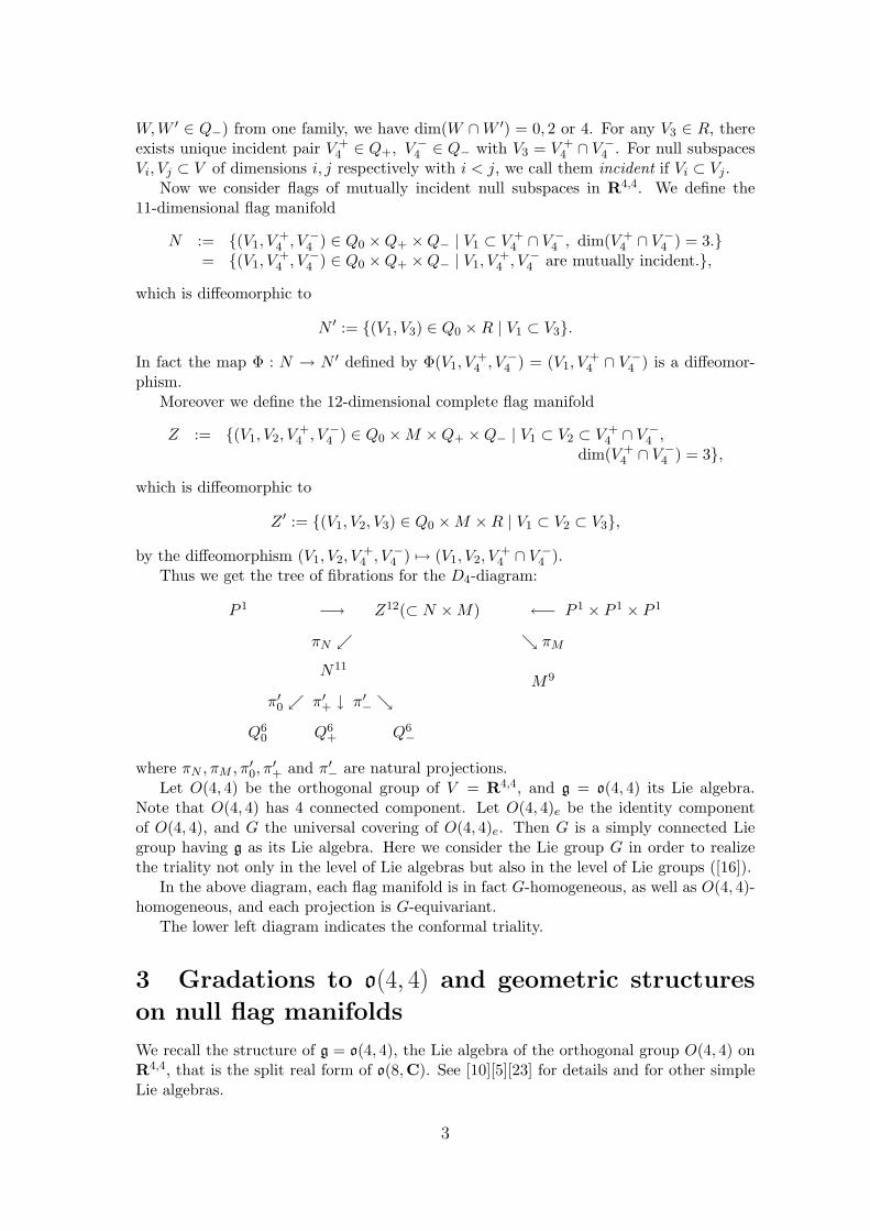
4 ).Thus we get the tree of fibrations for the D4-diagram:

P 1 −→ Z12(⊂ N × M) ←− P 1 × P 1 × P 1

πN πM

N11

π′0 π′

+ ↓ π′−

Q60 Q6

+ Q6−

M9

where πN , πM , π′0, π

′+ and π′

− are natural projections.Let O(4, 4) be the orthogonal group of V = R4,4, and g = o(4, 4) its Lie algebra.

Note that O(4, 4) has 4 connected component. Let O(4, 4)e be the identity componentof O(4, 4), and G the universal covering of O(4, 4)e. Then G is a simply connected Liegroup having g as its Lie algebra. Here we consider the Lie group G in order to realizethe triality not only in the level of Lie algebras but also in the level of Lie groups ([16]).

In the above diagram, each flag manifold is in fact G-homogeneous, as well as O(4, 4)-homogeneous, and each projection is G-equivariant.

The lower left diagram indicates the conformal triality.

3 Gradations to o(4, 4) and geometric structures

on null flag manifolds

We recall the structure of g = o(4, 4), the Lie algebra of the orthogonal group O(4, 4) onR4,4, that is the split real form of o(8,C). See [10][5][23] for details and for other simpleLie algebras.

3

With respect to a basis e1, . . . , e8 of R4,4 with inner products (ei|e9−j) = 12δij , 1 ≤

i, j ≤ 8, we have

o(4, 4) = A ∈ gl(8,R) | tAK + KA = O,= A = (aij) ∈ gl(8,R) | a9−j,9−i = −aij , 1 ≤ i, j ≤ 8,

where K = (kij) is the 8 × 8-matrix defined by ki,9−j = 12δij . Let

h := g0 = 〈 εi(Eii − E9−i,9−i) | εi ∈ R, 1 ≤ i ≤ 4 〉

be a Cartan subalgebra of g. Then the root system is given by ±εi ± εj , 1 ≤ i < j ≤ 4,and g is decomposed, over R, into the direct sum of root spaces

gεi−εj = 〈Ei,j − E9−j,9−i〉R, gεi+εj = 〈Ei,9−j − Ej,9−i〉R,

g−εi+εj = 〈Ej,i − E9−i,9−j〉R, g−εi−εj = 〈E9−j,i − E9−i,j〉R,

(1 ≤ i < j ≤ 4).The simple roots are given by

α1 := ε1 − ε2, α2 := ε2 − ε3, α3 := ε3 − ε4, α4 := ε3 + ε4.

(The numbering of simple roots is the same as in [4] and is slightly different from [16].)By labeling the root just on the left-upper-half part, we illustrate the structure of g:

ε1 α1 α1 + α2 α1 + α2 α1 + α2 α1 + α2 α1 + 2α2 0+α3 +α4 +α3 + α4 +α3 + α4

−α1 ε2 α2 α2 + α3 α2 + α4 α2 + α3 0+α4

−α1 − α2 −α2 ε3 α3 α4 0

−α1 − α2 −α2 − α3 −α3 ε4 0−α3

−α1 − α2 −α2 − α4 −α4 0 −ε4

−α4

−α1 − α2 −α2 − α3 0 −ε3

−α3 − α4 −α4

−α1 − 2α2 0 −ε2

−α3 − α4

0 −ε1

The Borel subalgebra is given by g≥0 = g0 ⊕∑

α>0 gα, the sum of Cartan subalgebrah = g0 and positive root spaces gα with respect to the simple root system α1, α2, α3, α4.

We take parabolic subalgebras g1, g2, g3, g4, where gi is the sum of g≥0 and all gα fora negative root α without αi-term. For instance,

g1 = 〈Eij − E9−j,9−i | 2 ≤ j ≤ 7, 1 ≤ i ≤ 8 − j 〉R + 〈E11 − E88〉R.

Moreover we have a parabolic subalgebra

g134 := g1 ∩ g3 ∩ g4 = g≥0 ⊕ g−α2 .

4

Let Ad : G → GL(g) denote the adjoint representation, B (resp. Gi) the normalizer inG under Ad of the subalgebra g≥0 (resp. the subalgebras gi, i = 1, 2, 3, 4). Then B (resp.Gi) has g≥0 (resp. gi) as its Lie algebra. The subgroup G134 := G1 ∩ G3 ∩ G4 has g134

as its Lie algebra. Then the flag manifolds Z,Q0,M,Q+, Q− and N are G-homogeneousspaces with isotropy groups B,G1, G2, G3, G4 and G134 respectively. We have

Z = G/B, Q0 = G/G1, M = G/G2, Q+ = G/G3, Q− = G/G4, N = G/G134.

Define the linear isomorphisms σ, τ : h∗ → h∗ on the dual space h∗ = 〈ε1, ε2, ε3, ε4〉R =〈α1, α2, α3, α4〉R of the Cartan subalgebra h by

σ(α1) = α3, σ(α2) = α2, σ(α3) = α4, σ(α4) = α1,

andτ(α1) = α1, τ(α2) = α2, τ(α3) = α4, τ(α4) = α3,

which induce Lie algebra isomorphisms σ, τ : g → g, expressed by the same letters,satisfying

σ(g±α1) = g±α3 , σ(g±α2) = g±α2 , σ(g±α3) = g±α4 , σ(g±α4) = g±α1 ,

andτ(g±α1) = g±α1 , τ(g±α2) = g±α2 , τ(g±α3) = g±α4 , τ(g±α4) = g±α3 .

The isomorphisms σ, τ are of order 3, 2 respectively. Thus g has S3-symmetry. Since G,the universal covering of O(4, 4)e, is simply connected, the S3-symmetry on g lifts to theS3-symmetry of G. In particular the associated isomorphism σ : G → G satisfies

σ(B) = B, σ(G1) = G3, σ(G2) = G2, σ(G3) = G4, σ(G4) = G1, σ(G134) = G134.

Thus, in particular, we have induced diffeomorphisms Q0∼= Q+

∼= Q−.The null quadric Q0 ⊂ P (V ) = P (R4,4) has the canonical conformal structure of type

(3, 3). In fact, for each V1 ∈ Q0, consider V ⊥1 ⊂ V = R4,4. Then the tangent space

TV1Q0 is isomorphic to V ⊥1 /V1, up to similarity transformation. Therefore the metric on

V induces the canonical conformal structure on Q0 of signature (3, 3). In other words,the conformal structure on Q0 is defined by the quadric tangent cone Cx of the Schubertvariety

Sx := W1 ∈ Q0 | W1 ⊂ V ⊥1 = P (V ⊥

1 ) ∩ Q0 ⊂ Q0,

for each x = V1 ∈ Q0.Also Q+ (resp. Q−) has a conformal structure of type (3, 3). In fact, for each y =

V ±4 ∈ Q±, the Schubert variety

S±y := W4 ∈ Q± | W4 ∩ V ±

4 6= 0 ⊂ Q±

induces invariant quadratic cone field (conformal structure) C±y on Q± defined by the

Pfaffian, respectively. The triality Q0∼= Q+

∼= Q− preserves the conformal structures.

Now we turn to construct the invariant differential systems on null flag manifolds.Let

g−1 := g−α1 ⊕ g−α2 ⊕ g−α3 ⊕ g−α4 .

The subspaceg≥−1 = g−1 ⊕ g≥0 = g134 + g2

5

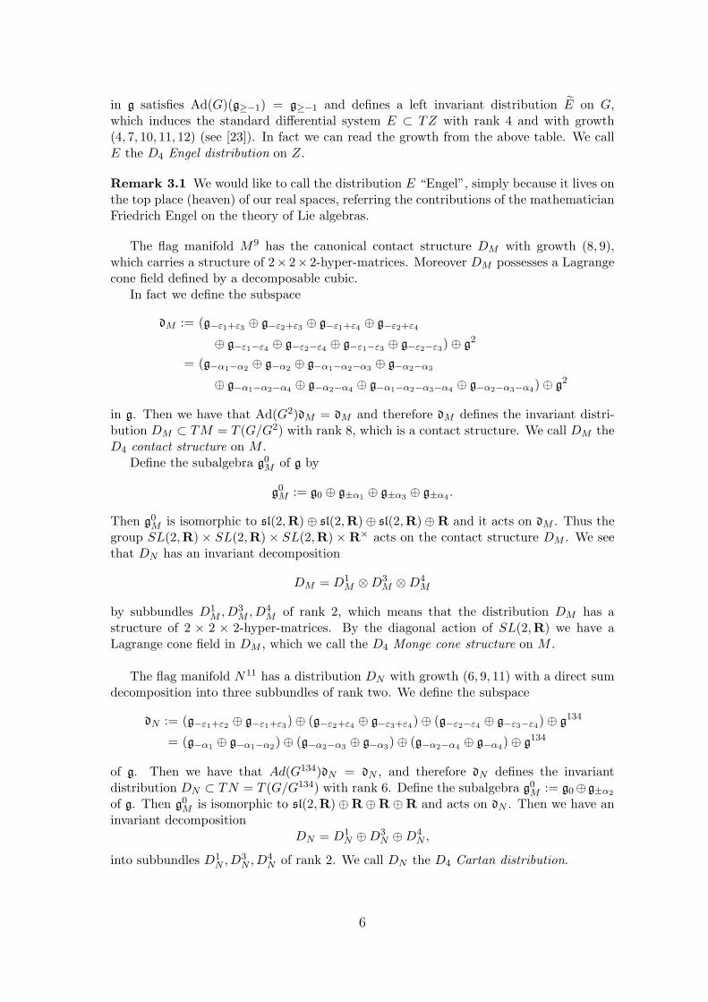
in g satisfies Ad(G)(g≥−1) = g≥−1 and defines a left invariant distribution E on G,which induces the standard differential system E ⊂ TZ with rank 4 and with growth(4, 7, 10, 11, 12) (see [23]). In fact we can read the growth from the above table. We callE the D4 Engel distribution on Z.

Remark 3.1 We would like to call the distribution E “Engel”, simply because it lives onthe top place (heaven) of our real spaces, referring the contributions of the mathematicianFriedrich Engel on the theory of Lie algebras.

The flag manifold M9 has the canonical contact structure DM with growth (8, 9),which carries a structure of 2× 2× 2-hyper-matrices. Moreover DM possesses a Lagrangecone field defined by a decomposable cubic.

In fact we define the subspace

dM := (g−ε1+ε3 ⊕ g−ε2+ε3 ⊕ g−ε1+ε4 ⊕ g−ε2+ε4

⊕ g−ε1−ε4 ⊕ g−ε2−ε4 ⊕ g−ε1−ε3 ⊕ g−ε2−ε3) ⊕ g2

= (g−α1−α2 ⊕ g−α2 ⊕ g−α1−α2−α3 ⊕ g−α2−α3

⊕ g−α1−α2−α4 ⊕ g−α2−α4 ⊕ g−α1−α2−α3−α4 ⊕ g−α2−α3−α4) ⊕ g2

in g. Then we have that Ad(G2)dM = dM and therefore dM defines the invariant distri-bution DM ⊂ TM = T (G/G2) with rank 8, which is a contact structure. We call DM theD4 contact structure on M .

Define the subalgebra g0M of g by

g0M := g0 ⊕ g±α1 ⊕ g±α3 ⊕ g±α4 .

Then g0M is isomorphic to sl(2,R) ⊕ sl(2,R) ⊕ sl(2,R) ⊕ R and it acts on dM . Thus the

group SL(2,R) × SL(2,R) × SL(2,R) × R× acts on the contact structure DM . We seethat DN has an invariant decomposition

DM = D1M ⊗ D3

M ⊗ D4M

by subbundles D1M , D3

M , D4M of rank 2, which means that the distribution DM has a

structure of 2 × 2 × 2-hyper-matrices. By the diagonal action of SL(2,R) we have aLagrange cone field in DM , which we call the D4 Monge cone structure on M .

The flag manifold N11 has a distribution DN with growth (6, 9, 11) with a direct sumdecomposition into three subbundles of rank two. We define the subspace

dN := (g−ε1+ε2 ⊕ g−ε1+ε3) ⊕ (g−ε2+ε4 ⊕ g−ε3+ε4) ⊕ (g−ε2−ε4 ⊕ g−ε3−ε4) ⊕ g134

= (g−α1 ⊕ g−α1−α2) ⊕ (g−α2−α3 ⊕ g−α3) ⊕ (g−α2−α4 ⊕ g−α4) ⊕ g134

of g. Then we have that Ad(G134)dN = dN , and therefore dN defines the invariantdistribution DN ⊂ TN = T (G/G134) with rank 6. Define the subalgebra g0

M := g0 ⊕g±α2

of g. Then g0M is isomorphic to sl(2,R) ⊕ R ⊕ R ⊕ R and acts on dN . Then we have an

invariant decompositionDN = D1

N ⊕ D3N ⊕ D4

N ,

into subbundles D1N , D3

N , D4N of rank 2. We call DN the D4 Cartan distribution.

6

Remark 3.2 We can compare the above mentioned facts with G2-diagram: We considerthe purely imaginary split octonions ImO′ with the inner product of type (3, 4) and con-sider the null projective space N5 (resp. the null Grassmannian M5, the flag manifold Z6)which consists of 1-dimensional null subalgebras (resp. 2-dimensional null subalgebras,the incident pairs of 1-dimensional null subalgebras and 2-dimensional null subalgebras)for the multiplication on the split octonions O′. The flag manifold Z has the Engel dis-tribution with growth (2, 3, 4, 5, 6), N5 has a distribution with growth (2, 3, 5), and thenull projective space M5 has a contact structure with growth (4, 5) with a cubic Lagrangecone field ([14])．

4 D4-triality and singularities of null tangent sur-

faces

We consider the canonical projections

π0 = π′0 πN : Z −→ Q0, π+ = π′

+ πN : Z −→ Q+, π− = π′− πN : Z −→ Q−,

and the diagramZ12 πM−−−−→ M9

π0 π+ ↓ π−

Q60 Q6

+ Q6−

induced by D4 Dynkin diagram.The D4 Engel distribution E on Z is described from the tree of fibrations, by

E = (kerπ0∗ ∩ kerπ+∗ ∩ kerπ−∗) ⊕ kerπM∗ ⊂ TZ,

which is of rank 4. See the definition of E as the standard differential system for o(4, 4)in §3.

A curve f : I → Z on Z is called E-integral if it is tangent to E, namely, if f∗(TI) ⊂E(⊂ TZ).

Definition 4.1 For the given (indefinite) conformal structure Cxx∈Q0 on Q0, we call acurve γ : I → Q0 a null curve if

γ′(t) ∈ Cγ(t), (t ∈ I).

A geodesic on Q0 is called a null geodesic if it is a null curve.A surface F : U → Q0 is called a null surface if

F∗(TuU) ⊂ CF (u), (u ∈ U).

The same definition is applied also to Q±.

Proposition 4.2 (Guillemin-Sternberg [9]) The null geodesics on Q0 for the conformalstructure on Q0 are given by null lines, namely, projective lines on Q0 ⊂ P (V ) = P (R4,4).

We will take null geodesics, namely, null lines as “tangent lines” for null curves in Q0.Note that any null line in Q0 is given by π0(π−1

M (V2)) for some V2 ∈ M . Then we are

7

naturally led to consider tangent surfaces of null curves in Q0, Q+ and Q−. For Q± wetake, as the family of “lines” in Q±,

π±(π−1M (V2)) = W4 ∈ Q± | V2 ⊂ W4, V2 ∈ M.

If we consider a special class of null curves which are projections of E-integral curvesf : I → Z to Q0, Q+ or Q−, then their tangent surfaces turn to be null surfaces in Q0, Q+

or Q− in the above sense. In fact we show later more strict results (Proposition 7.4).For M , we regard

πM (π−10 (V1) ∩ π−1

+ (V +4 ) ∩ π−1

− (V −4 )) = W2 | V1 ⊂ W2 ⊂ V +

4 ∩ V −4 , (V1, V

+4 , V −

4 ) ∈ N,

as lines in M .We will give the explicit classification of singularities of “tangent surfaces” in the

viewpoint of geometry of D4-triality:

Theorem 4.3 (Triality of singularities.) For a generic E-integral curve f : I −→ Z, thesingularities of tangent surfaces, to the curves γ0 = π0 f, γ+ = π+ f, γ− = π− f, γM =πM f on Q0, Q+, Q−,M,

Tan(γ0) = π0π−1M πMf(I)(⊂ Q0),

Tan(γ+) = π+π−1M πMf(I)(⊂ Q+), Tan(γ−) = π−π−1

M πMf(I)(⊂ Q−),Tan(γM ) = πM (π−1

0 π0f(I) ∩ π−1+ π+f(I) ∩ π−1

− π−f(I))(⊂ M),

at any point t ∈ I is classified, up to local diffeomorphisms, as follows:

Tan(γ0) Tan(γ+) Tan(γ−) Tan(γM )CE CE CE CE

OSW CE CE CECE OSW CE CECE CE OSW CEOM OM OM OSW

Here CE (resp. OSW, OM) means the cuspidal edge (resp. open swallowtail, open Mondsurface).

The cuspidal edge (resp. open swallowtail, open Mond surface) is defined as a diffeomor-phism class of the tangent surface-germ to a curve of type (1, 2, 3, · · · ) (resp. (2, 3, 4, 5, · · · ),(1, 3, 4, 5, · · · )) in an affine space. The type of a curve is the strictly increasing sequenceof orders (degrees of initial terms) of components in an appropriate system of linear co-ordinates. Their normal forms are given as follows:

CE : (u, t) 7→ (u, t2 − 2ut, 2t3 − 3ut2, 0, 0, 0), (R2, 0) → (R6, 0),(u, t) 7→ (u, t2 − 2ut, 2t3 − 3ut2, 0, 0, 0, 0, 0, 0), (R2, 0) → (R9, 0),

OSW : (u, t) 7→ (u, t3 − 3ut, t4 − 2ut2, 3t5 − 5ut3, 0, 0), (R2, 0) → (R6, 0),(u, t) 7→ (u, t3 − 3ut, t4 − 2ut2, 3t5 − 5ut3, 0, 0, 0, 0, 0), (R2, 0) → (R9, 0),

OM : (u, t) 7→ (u, 2t3 − 3ut2, 3t4 − 4ut3, 4t5 − 5ut4, 0, 0), (R2, 0) → (R6, 0),

8

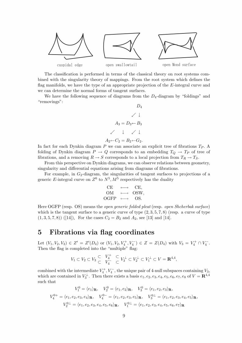
cuspidal edge open Mond surfaceopen swallowtail

The classification is performed in terms of the classical theory on root systems com-bined with the singularity theory of mappings. From the root system which defines theflag manifolds, we have the type of an appropriate projection of the E-integral curve andwe can determine the normal forms of tangent surfaces.

We have the following sequence of diagrams from the D4-diagram by “foldings” and“removings”:

D4

↓

A3 = D3←B3

↓ ↓

A2←C2 = B2←G2.

In fact for each Dynkin diagram P we can associate an explicit tree of fibrations TP . Afolding of Dynkin diagram P → Q corresponds to an embedding TQ → TP of tree offibrations, and a removing R → S corresponds to a local projection from TR → TS .

From this perspective on Dynkin diagrams, we can observe relations between geometry,singularity and differential equations arising from diagrams of fibrations.

For example, in G2-diagram, the singularities of tangent surfaces to projections of ageneric E-integral curve on Z6 to N5,M5 respectively has the duality

CE ←→ CE,OM ←→ OSW,

OGFP ←→ OS.

Here OGFP (resp. OS) means the open generic folded pleat (resp. open Shcherbak surface)which is the tangent surface to a generic curve of type (2, 3, 5, 7, 8) (resp. a curve of type(1, 3, 5, 7, 8)) ([14])．For the cases C2 = B2 and A2, see [13] and [14].

5 Fibrations via flag coordinates

Let (V1, V2, V3) ∈ Z ′ = Z ′(D4) or (V1, V2, V+4 , V −

4 ) ∈ Z = Z(D4) with V3 = V +4 ∩ V −

4 .Then the flag is completed into the “multiple” flag:

V1 ⊂ V2 ⊂ V3⊂ V +

4 ⊂⊂ V −

4 ⊂ V ⊥3 ⊂ V ⊥

2 ⊂ V ⊥1 ⊂ V = R4,4,

combined with the intermediate V +4 , V −

4 , the unique pair of 4-null subspaces containing V3,which are contained in V ⊥

3 . Then there exists a basis e1, e2, e3, e4, e5, e6, e7, e8 of V = R4,4

such that

V 01 = 〈e1〉R, V 0

2 = 〈e1, e2〉R, V 03 = 〈e1, e2, e3〉R,

V 0+4 = 〈e1, e2, e3, e4〉R, V 0−

4 = 〈e1, e2, e3, e5〉R, V 0⊥3 = 〈e1, e2, e3, e4, e5〉R,

V 0⊥2 = 〈e1, e2, e3, e4, e5, e6〉R, V 0⊥

1 = 〈e1, e2, e3, e4, e5, e6, e7〉R

9

and with inner products

(e1|e8) = 12 , (e2|e7) = 1

2 , (e3|e6) = 12 , (e4|e5) = 1

2 ,

other pairings being null. Such a basis e1, e2, e3, e4, e5, e6, e7, e8 of V = R4,4 is called anadapted basis for (V1, V2, V3) ∈ Z ′ = Z ′(D4) or (V1, V2, V

+4 , V −

4 ) ∈ Z = Z(D4). Then themetric on V is expressed via the coordinates x1, . . . , x8 associated to the above basis byds2 = dx1dx8 + dx2dx7 + dx3dx6 + dx4dx5.

For any curve f : I → Z, we can take a moving frame f : I → O(4, 4) such that f(t)is an adapted basis for f(t), which is called an adapted frame for f .

Remark 5.1 If we set

Z :=(V1, V2, V3, V4) | V1 ⊂ V2 ⊂ V3 ⊂ V4 ⊂ R4,4, dim(Vi) = i, V4 is null

,

then the projection π : Z → Z ′, π(V1, V2, V3, V4) = (V1, V2, V3) is a trivial double covering.In fact, if we set

Z± :=

(V1, V2, V3, V4) ∈ Z | V4 ∈ Q±

,

then Z = Z+ ∪Z−, disjoint union, and π|Z± : Z± → Z ′ is a diffeomorphism. As is seen asabove, we have an embedding Z into the complete flag manifold F1,2,3,4,5,6,7(R4,4).

Let us give local charts on Z ′, Z and Q0. Take another flag defined by

W 01 = 〈e8〉R, W 0

2 = 〈e8, e7〉R, W 03 = 〈e8, e7, e6〉R,

W 0+4 = 〈e8, e7, e6, e5〉R, W 0−

4 = 〈e8, e7, e6, e4〉R, W 0⊥3 = 〈e8, e7, e6, e5, e4〉R,

W 0⊥2 = 〈e8, e7, e6, e5, e4, e3〉R, W 0⊥

1 = 〈e8, e7, e6, e5, e4, e3, e2〉R,

and take the open neighborhood

U ′ = (V1, V2, V3) ∈ Z ′ | V1 ∩ W 0⊥1 = 0, V2 ∩ W 0⊥

2 = 0, V3 ∩ W 0⊥3 = 0

of (V 01 , V 0

2 , V 03 ) in Z ′. Then, for any (V1, V2, V3) ∈ U ′, there exist unique f1, f2, f3 ∈ V3

such that f1 forms a basis of V1, f1, f2 form a basis of V2 and f1, f2, f3 form a basis of V3

respectively and they are of formf1 = e1 + x21e2 + x31e3 + x41e4 + x51e5 + x61e6 + x71e7 + x81e8

f2 = e2 + x32e3 + x42e4 + x52e5 + x62e6 + x72e7 + x82e8

f3 = e3 + x43e4 + x53e5 + x63e6 + x73e7 + x83e8

for some xij ∈ R. Then we have

(f1|f1) = x81 + x21x71 + x31x61 + x41x51 = 0,2(f1|f2) = x82 + x21x72 + x31x62 + x41x52 + x51x42 + x61x32 + x71 = 0,2(f1|f3) = x83 + x21x73 + x31x63 + x41x53 + x51x43 + x61 = 0,(f2|f2) = x72 + x32x62 + x42x52 = 0,

2(f2|f3) = x73 + x32x63 + x42x53 + x52x43 + x62 = 0,(f3|f3) = x63 + x43x53 = 0.

Therefore we see that

(x21, x31, x41, x51, x61, x71, x32, x42, x52, x62, x43, x53)

10

is a chart on U ′ ⊂ Z ′.Moreover we take

f4 = e4 + x54e5 + x64e6 + x74e7 + x84e8,

from V +4 so that f1, f2, f3, f4 form a basis of V +

4 , and take

f5 = x45e4 + e5 + x65e6 + x75e7 + x85e8,

from V −4 so that f1, f2, f3, f5 form a basis of V −

4 . We have

2(f1|f4) = x84 + x21x74 + x31x64 + x41x54 + x51 = 0,2(f2|f4) = x74 + x32x64 + x42x54 + x52 = 0,2(f3|f4) = x64 + x43x54 + x53 = 0,(f4|f4) = x54 = 0,

2(f1|f5) = x85 + x21x75 + x31x65 + x41 + x51x45 = 0,2(f2|f5) = x75 + x32x65 + x42 + x52x45 = 0,2(f3|f5) = x65 + x43 + x53x45 = 0,(f4|f5) = x45 = 0.

We set

U := (V1, V2, V+4 , V −

4 ) ∈ Z | V1 ∩ W 0⊥1 = 0, V2 ∩ W 0⊥

2 = 0, V ±4 ∩ W 0±

4 = 0,

Consider the diffeomorphism Φ : Z → Z ′ defined by Φ(V1, V2, V+4 , V −

4 ) = (V1, V2, V+4 ∩

V −4 )(= (V1, V2, V3)). Then Φ(U) = U ′. After replacing x43, x53 by x64, x65, we have a

chart(x21, x31, x41, x51, x61, x71, x32, x42, x52, x62, x64, x65)

on U = Φ−1(U ′) ⊂ Z and the mapping Φ is locally given by just x53 = −x64, x43 = −x65.In fact other components are calculated as follows:

x81 = −x71x21 − x61x31 − x51x41,x72 = −x62x32 − x52x42,x82 = x62(x32x21 − x31) + x52(x42x21 − x41) − x51x42 − x61x32 − x71,x43 = −x65,x53 = −x64,x63 = −x65x64,x73 = x65x64x32 + x64x42 + x65x52 − x62,x83 = x65x64(x31 − x32x21) + x64(x41 − x42x21) + x65(x51 − x52x21) − x61 + x62x21,x74 = −x64x32 − x52,x84 = x64(x32x21 − x31) + x52x21 − x51,x75 = −x65x32 − x42,x85 = x65(x32x21 − x31) + x42x21 − x41.

Now we will explicitly describe π0, π+, π− and πM locally on U ⊂ Z.It is easy to describe π0 in terms of our charts: Consider the open neighborhood of

V 01 ∈ Q0:

U0 := V1 ∈ Q0 | V1 ∩ W 0⊥1 = 0.

Then, using the above notations, (x21, x31, x41, x51, x61, x71) provides a chart on U0 ⊂ Q0.Moreover π0 : U → U0 is given by

(x21, x31, x41, x51, x61, x71, x32, x42, x52, x62, x64, x65) 7→ (x21, x31, x41, x51, x61, x71).

11

We describe πM . Set

UM := V2 ∈ M | V2 ∩ W 0⊥2 = 0,

and take a basis of V2 ∈ M of formh1 = e1 +z31e3 + z41e4 + z51e5 + z61e6 + z71e7 + z81e8,h2 = e2 +z32e3 + z42e4 + z52e5 + z62e6 + z72e7 + z82e8.

Then we have a chart on UM ⊂ M by

(z31, z41, z51, z61, z71, z32, z42, z52, z62).

Using the modification h1 = f1−x21f2, h2 = f2, we have that the projection πM : U → UM

is given by

z31 = x31 − x32x21, z41 = x41 − x42x21, z51 = x51 − x52x21, z61 = x61 − x62x21,z71 = x71 + x62x32x21 + x52x42x21, z32 = x32, z42 = x42, z52 = x52, z62 = x62.

To describe π+, we set

U+ := V +4 ∈ Q+ | V +

4 ∩ W 0+4 = 0,

and take a basis of V +4 ∈ U+ of form

g1 = e1 +y51e5 + y61e6 + y71e7 + y81e8,g2 = e2 +y52e5 + y62e6 + y72e7 + y82e8,g3 = e3 +y53e5 + y63e6 + y73e7 + y83e8,g4 = e4 +y54e5 + y64e6 + y74e7 + y84e8.

Note that y54 = 0. Then we have a chart on U+ by

(y51, y61, y71, y52, y62, y64).

We use the modificationsg1 = f1 − x21f2 − (x31 − x32x21)f3 − (x41 − x42x21 − x43(x31 − x32x21))f4,g2 = f2 − x32f3 − (x42 − x43x32)f4,g3 = f3 − x43f4.

Then the projection π+ : U → U+ is described in terms of our charts, by

y51 = x51 − x52x21 + x64(x31 − x32x21),y61 = x61 − x62x21 − x64(x41 − x42x21),y71 = x71 + x62x31 + x52x41 − x64(x42x31 − x41x32),y52 = x52 + x64x32,y62 = x62 − x64x42,y64 = x64.

To describe π−, similarly we set

U− := V −4 ∈ Q− | V −

4 ∩ W 0−4 = 0,

12

and take a basis of V −4 ∈ U−:

g1 = e1 + y41e4 +y61e6 + y71e7 + y81e8,g2 = e2 + y42e4 +y62e6 + y72e7 + y82e8,g3 = e3 +y43e4 +y63e6 + y73e7 + y83e8,g5 = y45e4 +e5 +y65e6 + y75e7 + y85e8.

Note that y45 = 0. Then a chart on U− is given by

(y41, y61, y71, y42, y62, y65).

Use the modificationsg1 = f1 − x21f2 − (x31 − x32x21)f3 − (x51 − x52x21 − x53(x31 − x32x21))f5,g2 = f2 − x32f3 − (x52 − x53x32)f5,g3 = f3 − x53f5.

Then the projection π− : U → U− is given by

y41 = x41 − x42x21 + x65(x31 − x32x21),y61 = x61 − x62x21 − x65(x51 − x52x21),y71 = x71 + x62x31 + x51x42 − x65(x51x32 − x52x31),y42 = x42 + x65x32,y62 = x62 − x65x52,y65 = x65.

6 The Engel system via flag coordinates

Recall thatE = (kerπ0∗ ∩ kerπ+∗ ∩ kerπ−∗) ⊕ kerπM∗ ⊂ TZ.

First we show

Lemma 6.1 Let f = (V1, V2, V+4 , V −

4 ) ∈ Z and e = (e1, e2, e3, e4, e5, e6, e7, e8) be anadapted basis for f (see §5). For each tangent vector v ∈ TfZ, the following conditionsare equivalent to each other:(1) The tangent vector v belongs to Ef .(2) There exists a representative c : (R, 0) → (Z, f), c(t) = (V1(t), V2(t), V +

4 (t), V −4 (t)) of

the tangent vector v, and framing

V1(t) = 〈f1(t)〉R, V2(t) = 〈f1(t), f2(t)〉R,

V +4 (t) = 〈f1(t), f2(t), f3(t), f4(t)〉R, V −

4 (t) = 〈f1(t), f2(t), f3(t), f5(t)〉R,

by a curve-germ f : (R, 0) → GL(R4,4),

f(t) = (f1(t), f2(t), f3(t), f4(t), f5(t), f6(t), f7(t), f8(t)),

with f(0) = e, which satisfies that f ′1(0) ∈ V2, f

′2(0) ∈ V +

4 ∩ V −4 .

(3) The tangent vector v satisfies that

π0∗v ∈ TV1(G1(V2)) and πM∗v ∈ TV2(G2(V +4 ∩ V −

4 )).

13

Proof . (1) ⇒ (2): Let v = w + u,w ∈ kerπ0∗ ∩ kerπ+∗ ∩ kerπ−∗, u ∈ kerπM∗. Take aframe

g(t) = (g1(t), g2(t), g3(t), g4(t), g5(t), g6(t), g7(t), g8(t))

of V such that g(t) defines the tangent vector u at t = 0 and that 〈g1(t), g2(t)〉R = V2.Take a frame

h(t) = (h1(t), h2(t), h3(t), h4(t), h5(t), h6(t), h7(t), h8(t)))

such that h(t) defines the tangent vector w at t = 0 and that

〈h1(t)〉R = V1, 〈h1(t), h2(t), h3(t), h4(t)〉R = V +4 , 〈h1(t), h2(t), h3(t), h5(t)〉R = V −

4

with g(0) = h(0) = e. Then the curve f(t) := g(t) + h(t) − g(0) represents v. Moreoverf ′1(0) = g′1(0) + h′

1(0) ∈ V2, f′2(0) = g′2(0) + h′

2(0) ∈ V +4 ∩ V −

4 .The assertion (2) ⇒ (3) is clear.(3) ⇒ (1): We take a frame f(t) = (f1(t), f2(t), f3(t), f4(t), f5(t)) for v such that f1(t) ∈V2, f2(t) ∈ V3 = V +

4 ∩ V −4 . Write

f1 = e1 + x21e2,f2 = e2 + x32e3,f3 = e3 − x65e4 − x64e5 + x63e6 + x73e7 + x83e8,f4 = e4 + x64e6 + x74e7 + x84e8,f5 = e5 + x65e6 + x75e7 + x85e8,

with functions xij = xij(t) with xij(0) = 0. Then we have x83 = −x21x73, x84 =−x21x74, x85 = −x21x75, x73 = −x32x63, x74 = −x32x64, x75 = −x32x65. Thereforex′

83(0) = 0, x′84(0) = 0, x′

85(0) = 0, x′73(0) = 0, x′

74(0) = 0, x′75(0) = 0. We define g(t)

and h(t) by g1 = e1,g2 = e2 + x32e3,g3 = e3,g4 = e4,g5 = e5,

and h1 = e1 + x21e2,h2 = e2,h3 = e3 − x65e4 − x64e5 + x63e6,h4 = e4 + x64e6,h5 = e5 + x65e6.

Let w ∈ TfZ (resp. u ∈ TfZ) be tangent vectors defined by the curve g(t) (resp. h(t))at t = 0. Then w (resp. u) belongs to ker π0∗ ∩ kerπ+∗ ∩ kerπ−∗ (resp. to ker πM∗). Setk(t) = g(t) + h(t). Then we see that f ′(0) = k′(0) = g′(0) + h′(0). Thus we have thatv = w + u ∈ (kerπ0∗ ∩ kerπ+∗ ∩ kerπ−∗) ⊕ kerπM∗. 2

Regarding Lemma 6.1, the differential system E ⊂ TZ is given by the conditionf ′1 ∈ 〈f1, f2〉R, f ′

2 ∈ 〈f1, f2.f3〉R. In terms of component functions xij , the condition isgiven by

(x′21, x

′31, x

′41, x

′51, x

′61, x

′71, x

′81) = p(1, x32, x42, x52, x62, x72, x82)

and(x′

32, x′42, x

′52, x

′62, x

′72, x

′82) = q(1, x43, x53, x63, x73, x83),

14

for some p, q ∈ R. Then p = x′21, q = x′

32. Therefore we have that the differential systemE ⊂ TZ on our coordinate neighborhood U is given by

dxi1 = xi2dx21(3 ≤ i ≤ 8), dxj2 = xj3dx32(4 ≤ j ≤ 8).

We introduce a weight wij ∈ R on each component xij . From the above equations forE, we impose the relations

wi1 = wi2 + w21(3 ≤ i ≤ 8), wj2 = wj3 + w32(4 ≤ j ≤ 8).

Then the weights of all components xij are well-defined and they are explicitly expressedby w21, w32, w65 and w64. Moreover we have

Lemma 6.2 (Triality of weights.) The projection π0, π+, π− and πM are weighted homo-geneous mappings respectively. The weights of components of the projections π0, π+, π−to Q0, Q+, Q− are given by the following table:

Q0 Q+ Q−w21 w65 w64

w32 + w21 w65 + w32 w64 + w32

w64 + w32 + w21 w65 + w32 + w21 w64 + w32 + w21

w65 + w32 + w21 w65 + w64 + w32 w65 + w64 + w32

w65 + w64 + w32 + w21 w65 + w64 + w32 + w21 w65 + w64 + w32 + w21

w65 + w64 + 2w32 + w21 w65 + w64 + 2w32 + w21 w65 + w64 + 2w32 + w21

The weights of components of the projection πM to M are given by

w32, w32 + w21, w65 + w32, w64 + w32,w65 + w32 + w21, w64 + w32 + w21, w65 + w64 + w32,

w65 + w64 + w32 + w21, w65 + w64 + 2w32 + w21.

Remark 6.3 We observe that the formula of weights coincides with the formula of neg-ative (or positive) roots of D4 (see [4] for example). In fact, given a simple root systemα1, α2, α3, α4, we identify −α1,−α2,−α3,−α4 with w21, w32, w65, w64. Then the weight wof a component for a negative root α is given by w = m1w21 + m2w32 + m3w65 + m4w64

if α = −m1α1 − m2α2 − m3α3 − m4α4. See the following D4 diagram with weightsw21, w32, w65, w64 at appropriate positions:

w65

w21 —– w32

w64

Then we have the orders of flag coordinates for generic E-integral curves, and normalforms of singularities appeared in tangent surfaces.

15

Lemma 6.4 Let f : I → Z be a generic E-integral curve. Then, for any t0 ∈ I andfor any flag chart (xij) on Z centered at f(t0), the sets of orders on components for theprojections π0f, π+f, π−f, πMf are given as in the following table:

(w21, w65, w64, w32) π0f π+f π−f πMf

(1, 1, 1, 1) 1, 2, 3, 3, 4, 5∗ 1, 2, 3, 3, 4, 5∗ 1, 2, 3, 3, 4, 5∗ 1, 2, 2, 2, 3, 3, 3, 4, 5∗

(2, 1, 1, 1) 2, 3, 4, 4, 5, 6 1, 2, 4, 3, 5, 6 1, 2, 4, 3, 5, 6 1, 3, 2, 2, 4, 4, 3, 5, 6(1, 2, 1, 1) 1, 2, 3, 4, 5, 6 2, 3, 4, 4, 5, 6 1, 2, 3, 4, 5, 6 1, 2, 3, 2, 4, 3, 4, 5, 6(1, 1, 2, 1) 1, 2, 4, 3, 5, 6 1, 2, 3, 4, 5, 6 2, 3, 4, 4, 5, 6 1, 2, 2, 3, 3, 4, 4, 5, 6(1, 1, 1, 2) 1, 3, 4, 4, 5, 7 1, 3, 4, 4, 5, 7 1, 3, 4, 4, 5, 7 2, 3, 3, 3, 4, 4, 4, 5, 7

where 5∗ means 5 or 6 on an isolated points.

Remark 6.5 From the formula on weights of components, we can estimate the ordersof component functions of E-integral curves. However it is possible that the orders ofsome components become higher than expected by accidental cancelings of leading terms.Therefore, in order to determine the exact order of each component of generic curves,we need the explicit local expressions of the projections π0, π+, π−, πM and the differentialsystem E ⊂ TZ.

Proof of Lemma 6.4. As we have seen in the above arguments, all components of π0 f(resp. π+f, π−f, πM f) are obtained just from the four components x21f, x65f, x64f, x32 f by differentiations, multiplications, summations and integrations. We can spellout, from the explicit expression of components obtained in §5, which component mayhave higher order than expected. For example, since (x52 f)′ = (x53 f)(x32 f)′, we seex52 f =

∫(x53 f)(x32 f)′dt. Therefore ord(x52 f) = ord(x53 f) + ord(x32 f). As

another example, for the component z31f = (x31−x32x21)f of πM , we have (z31f)′ =(x31 − x32x21) f′ = −(x32 f)′(x21 f). Therefore z31 f = −

∫(x32 f)′(x21 f)dt

and ord(z31 f) = ord((x32 f) + ord(x21 f).By the ordinary transversality theorem, we have, generically, just four cases where

(ord(x21 f), ord(x65 f), ord(x64 f), ord(x32 f)) is equal to

(1, 1, 1, 1), (2, 1, 1, 1), (1, 2, 1, 1), (1, 1, 2, 1), (1, 1, 1, 2),

respectively. The last four cases occur just on isolated points, where the orders of allcomponents are equal to the weights of components. In the first case, the order of onecomponent may increase by one from the weight of the component accidentally on anisolated points. Thus we have the above table. 2

Proof of Theorem 4.3: We use several results proved in [11]. If the set of orders contains1, 2, 3 (resp. 2, 3, 4, 5, 1, 3, 4, 5), then the tangent surface to the projection of the Engelintegral curve is locally diffeomorphic to the cuspidal edge (resp. the open swallowtail, theopen Mond surface) in (R6, 0) or (R9, 0). This is proved essentially by the versality of thecuspidal edge (resp. the open swallowtail, the open Mond surface) as an “opening” of thefold map (resp. the Whitney’s cusp, the beak-to beak map) (R2, 0) → (R2, 0). For exam-ple, we show one case where the set of orders of components is given by 1, 2, 3, 3, 4, 5.Then the projection of the Engel integral curve is locally expressed by c : (R, 0) → (R6, 0)

16

with components

x1(t) = a1t + · · · ,x2(t) = a2t

2 + · · · ,x3(t) = a3t

3 + · · · ,x4(t) = a4t

3 + · · · ,x5(t) = a5t

4 + · · · ,x6(t) = a6t

5 + · · · .

where ai 6= 0, 1 ≤ i ≤ 6 and · · · means higher order terms. Then, by a local diffeomor-phism on (R, 0) and a linear transformation on (R6, 0) the curve is transformed into acurve c : (R, 0) → (R6, 0) with components

x1(t) = t, x2(t) = t2 + ϕ2(t), x3(t) = t3 + ϕ3(t),x4(t) = t3 + ϕ4(t), x5(t) = t4 + ϕ5(t), x6(t) = t5 + ϕ6(t),

where ord(ϕ2) ≥ 3, ord(ϕ3) ≥ 4, ord(ϕ4) ≥ 4, ord(ϕ5) ≥ 5, ord(ϕ6) ≥ 6. The tangentsurface of c is parametrized by F (t, s) = c(t) + sc′(t), namely,

x1(t, s) = t + s, x2(t, s) = t2 + 2st + ϕ2(t) + sϕ′2(t),

x3(t, s) = t3 + 3st2 + ϕ3(t) + sϕ′3(t), x4(t, s) = t3 + 3st2 + ϕ4(t) + sϕ′

4(t),x5(t, s) = t4 + 4st3 + ϕ5(t) + sϕ′

5(t), x6(t, s) = t5 + 5st4 + ϕ6(t) + sϕ′6(t).

If we put u = t + s, then we have that F is diffeomorphic to a map-germ G : (R2, 0) →(R6, 0) with components

x1(t, u) = u, x2(t, u) = −t2 + 2ut + ψ2(t, u),x3(t, u) = −2t3 + 3ut2 + ψ3(t, u), x4(t, u) = −2t3 + 3ut2 + ψ4(t, u),x5(t, u) = −3t4 + 4ut3 + ψ5(t, u), x6(t, u) = −4t5 + 5ut4 + ψ3(t, u),

where ψi(t, u) = ϕi(t) + (u − t)ϕ′i(t). Now consider the set R of functions h(t, u) such

that ∂h∂t is a functional multiple of u − t. All components of G belong to R. We define

g, g : (R2, 0) → (R2, 0), by g(t, u) = (u,−t2 + 2ut + ψ2(t, u)) and g(t, u) = (u,−t2 + 2ut),both of which are diffeomorphic to the fold map. Then R coincides with Rg, the totalityof h : (R2, 0) → R such that dh is a functional linear combination of du and d(−t2 +2ut + ψ2(t, u)), and with Rg which is similarly defined. In this situation, we say that Gis an opening of g. We can show that any h ∈ R is a function on

G = (u,−t2 + 2ut,−2t3 + 3ut2),

which is a versal opening of g. Thus we see, in fact, that there exist functions

Φ2, Φ3, Φ4, Φ5, Φ6 : (R3, 0) → (R, 0)

on (R3, 0) with coordinates y1, y2, y3 such that

x1(t, u) = u, x2(t, u) = −t2 + 2ut + Φ2 G,

x3(t, u) = −2t3 + 3ut2 + Φ3 G, x4(t, u) = −2t3 + 3ut2 + Φ4 G,

x5(t, u) = Φ5 G, x6(t, u) = Φ6 G.

Then we see necessarily that ∂Φ2∂y2

(0) = 0, ∂Φ3∂y3

(0) = 0. Define a map-germ τ : (R6, 0) →(R6, 0) by

τ(y1, y2, y3, y4, y5, y6) = (y1, y2 + Φ2(y1, y2, y3), y3 + Φ3(y1, y2, y3),y3 + y4 + Φ4(y1, y2, y3), y5 + Φ5(y1, y2, y3), y6 + Φ6(y1, y2, y3)) .

17

Then we have that τ is a diffeomorphism-germ of (R6, 0) and G = τ (G, 0, 0, 0). ThusF is diffeomorphic to (G, 0, 0, 0), which is diffeomorphic to

(u, v) 7→ (u, v2, v3, 0, 0, 0),

the cuspidal edge in R6. Note that (G, 0, 0, 0) provides a normal form among tangentmappings.

On the notions of openings and versal openings, and related results, see [11]. We cantreat other cases similarly using Lemma 6.4. Thus we have Theorem 4.3. 2

7 D4 Cartan distributions and null frontals

We have defined in §3 the distribution DN ⊂ TN on the flag manifold N .

Definition 7.1 A mapping F : U → Q0 (resp. F : U → Q+, F : U → Q−) from a 2-dimensional manifold U is called a null frontal if there exists a DN -integral lift F : U → Nof F , i.e. which satisfies F∗(TxU) ⊂ (DN )

eF (x)and π′

0(F (x)) = F (x) (resp. π′+(F (x)) =

F (x), π′−(F (x)) = F (x)), for any x ∈ U .

Remark 7.2 In the above definition, if we can take F an immersion, then we call F anull front.

Recall that Q0, Q1, Q2 are endowed with conformal structures of type (3, 3) and wehave defined the notion of null surfaces (Definition 4.1).

Proposition 7.3(1) If F : U → Q0 ( resp. F : U → Q+, F : U → Q−) is a regular (immersive) nullsurface, then F is a null frontal.(2) If F : U → Q0 ( resp. F : U → Q+, F : U → Q−) is a null frontal, then F is a nullsurface.

As is mentioned in §4, we have the following:

Proposition 7.4 Let f : I → Z be an E-integral curve. Consider the projections γ0 =π0 f : I → Q0, γ+ = π+ f : I → Q+ and γ− = π− f : I → Q−. Then the tangentsurfaces F0 = Tan(γ0), F1 = Tan(γ+) and F− = Tan(γ−) are null frontals. In fact, thereexists a DN -integral lifting F0 of F0 (resp. F+ of F+, F− of F−) such that π+ F0 andπ− F0 (resp. π− F+ and π0 F+, π0 F− and π+ F−) are constant along tangentlines.

Note that DN is described, in terms of tree of fibrations, by

(kerπ′+∗ ∩ kerπ′

−∗) ⊕ (kerπ′0∗ ∩ kerπ′

−∗) ⊕ (kerπ′0∗ ∩ kerπ′

+∗) ⊂ TN.

To show Propositions 7.3 and 7.4, we need the following Lemma 7.5 which gives theequivalent descriptions of DN in different forms. The proof of Lemma 7.5 is similar toLemma 6.1 and we omit it.

18

Lemma 7.5 Let f = (V1, V+4 , V −

4 ) ∈ N . For each tangent vector v ∈ TfN , the followingconditions are equivalent to each other:(1) The tangent vector v belongs to (DN )f .(2) There exists a representative c : (R, 0) → (N, f), c(t) = (V1(t), V +

4 (t), V −4 (t)) of the

tangent vector v, and framing

V1(t) = 〈f1(t)〉R, V +4 (t) ∩ V −

4 (t) = 〈f1(t), f2(t), f3(t)〉R,

V +4 (t) = 〈f1(t), f2(t), f3(t), f4(t)〉R, V −

4 (t) = 〈f1(t), f2(t), f3(t), f5(t)〉R,

by a curve-germ f : (R, 0) → GL(R4,4),

f(t) = (f1(t), f2(t), f3(t), f4(t), f5(t), f6(t), f7(t), f8(t)),

which satisfies that f(0) is an adapted basis for some flag in π−1N (f) ⊂ Z, and that

f ′1(0) ∈ V +

4 ∩ V −4 , f ′

2(0), f ′3(0) ∈ (V +

4 ∩ V −4 )⊥.

(3) The tangent vector v satisfies that

π0∗v ∈ TV1(π0(π′−1+ V +

4 ∩ π′−1− V −

4 )),

π+∗v ∈ TV +4

(π+(π′−10 V1 ∩ π

′−1− V −

4 )), π−∗v ∈ TV −4

(π−(π′−10 V1 ∩ π

′−1+ V +

4 )).

Proof of Proposition 7.3:(1) Let v ∈ TxU . Suppose F∗(v) 6= 0. Then we have F∗(v) ∈ (DN )

eF (x). Take a curve

(V1(t), V +4 (t), V −

4 (t)) on N which represents, at t = 0, the tangent vector F∗(v) at F (x).Then f ′

1(0) ∈ V +4 (0) ∩ V −

4 (0). The vector f ′1(0) corresponds to F∗(v). Therefore we have

F∗(v) ∈ TF (x)(P (V +4 (0) ∩ V −

4 (0))) ⊂ TF (x)(P (V1(0))⊥ ∩ Q0) = CF (x).

(2) Regarding F (u, v) as a 1-dimensional subspace in V , we take a frame f(u, v) of F (u, v).Since F is regular,

f(u, v),∂f

∂u(u, v),

∂f

∂v(u, v)

are linearly independent and

V3(u, v) := 〈f,∂f

∂u,∂f

∂v〉R

is a null 3 space in V = R4,4, for any (u, v) ∈ U . Then by the partial differentiations withrespect to u, v of the equalities

(f |∂f

∂u) = 0, (f |∂f

∂v) = 0, (

∂f

∂u|∂f

∂u) = 0, (

∂f

∂u|∂f

∂v) = 0, (

∂f

∂v|∂f

∂v) = 0,

we have that∂2f

∂u2,

∂2f

∂u∂v,∂2f

∂v2∈ V3(u, v)⊥.

We set V1(u, v) = 〈f(u, v)〉R ⊂ V , and take the unique null 4-spaces V +4 (u, v), V −

4 (u, v)such that V3(u, v) = V +

4 (u, v) ∩ V −4 (u, v). Then we have that F : U → N defined by

F (u, v) = (V1(u, v), V +4 (u, v), V−(u, v))

19

is DN -integral by Lemma 7.4, and that π′0 F = F . Therefore F is a null frontal. 2

Proof of Proposition 7.4:Let f : I → Z, f(t) = (V1(t), V2(t), V +

4 (t), V −4 (t)) be an E-integral curve. Take a frame

f1(t) of V1(t), f1(t), f2(t) of V2(t), f1(t), f2(t), f3(t), f4(t) of V +4 (t) and f1(t), f2(t), f3(t), f5(t)

of V −4 (t). Then the curve γ0(t) is defined by the family V1(t). Consider, for each t ∈ I,

V1(t, s) = f1(t) + sf2(t), which can be regarded a projective line. By the conditionf ′1(t) ∈ V2(t), V1(t, s) gives the tangent line to γ at t, even when f1(t), f ′

1(t) are linearlydependent. Then F0 = Tan(γ0(t)) is given by F0(t, s) = V1(t, s) and s is the parameter oftangent lines. We define the lift F0 of F0 to N by

F0(t, s) := (V1(t, s), V +4 (t), V −

4 (t)).

We have that

∂

∂t(f1(t) + sf2(t)) = f ′

1(t) + sf ′2(t) ∈ V +

4 (t) ∩ V −4 (t),

∂

∂s(f1(t) + sf2(t)) = f2(t) ∈ V2(t) ⊂ V +

4 (t) ∩ V −4 (t),

and that∂

∂tf3(t) ∈ (V +

4 (t)∩V −4 (t))⊥,

∂

∂sf3(t) = 0. Thus we have that F0 is DN -integral by

Lemma 7.5. Therefore we have that F0 is a null frontal. Moreover (π+ F0)(t, s) = V +4 (t)

and (π− F0)(t, s) = V −4 (t) do not depend on s.

By the triality, we have the results also for F+ = Tan(γ+(t)) and F− = Tan(γ−(t)).In fact, under the diffeomorphism Φ : N → N ′, Φ(V1, V

+4 , V −

4 ) = (V1, V+4 ∩ V −

4 ),Φ F+ : I → N ′ is given by

Φ F+(t) = (V1(t), V3(t, s)), V3(t, s) := 〈f1(t), f2(t), f3(t) + sf5(t)〉R, (t, s) ∈ I × R,

and Φ F− : I → N ′ is given by

Φ F−(t) = (V1(t), V3(t, s)), V3(t, s) := 〈f1(t), f2(t), f3(t) + sf4(t)〉R, (t, s) ∈ I × R.

If we arrange to take an adapted frame f : I → O(4, 4),

f(t) = (f1(t), f2(t), f3(t), f4(t), f5(t), f6(t), f7(t), f8(t)),

for the Engel integral curve f : I → Z (see §5), then we may write

F+(t, s) = (V1(t), V +4 (t, s), V −

4 (t)), V +4 (t, s) := 〈f1(t), f2(t), f3(t) + sf5(t), f3(t)− sf6(t)〉R,

and

F−(t, s) = (V1(t), V +4 (t), V −

4 (t, s)), V −4 (t, s) := 〈f1(t), f2(t), f3(t) + sf4(t), f3(t)− sf6(t)〉R,

for any (t, s) ∈ I ×R. Therefore F+ (resp. F−) has a DN -integral lift F+ (resp. F−) suchthat π− F+ and π0 F+ (resp. π0 F− and π+ F−) do not depend on s 2

Let us describe DN in coordinates. To describe N ′ first, fix a complete flag as before

W 01 ⊂ W 0

2 ⊂ W 03

⊂ W 0+4 ⊂

⊂ W 0−4 ⊂

W 0⊥3 ⊂ W 0⊥

2 ⊂ W 0⊥1 ⊂ V = R4,4,

20

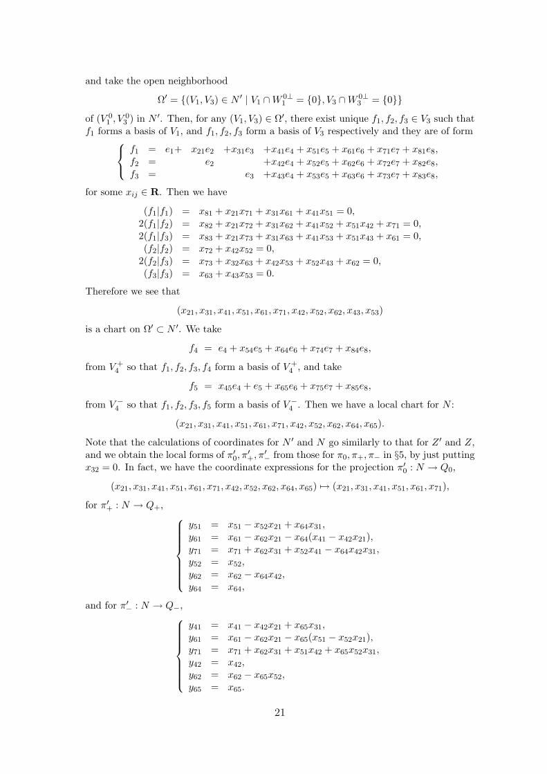
and take the open neighborhood

Ω′ = (V1, V3) ∈ N ′ | V1 ∩ W 0⊥1 = 0, V3 ∩ W 0⊥

3 = 0

of (V 01 , V 0

3 ) in N ′. Then, for any (V1, V3) ∈ Ω′, there exist unique f1, f2, f3 ∈ V3 such thatf1 forms a basis of V1, and f1, f2, f3 form a basis of V3 respectively and they are of form

f1 = e1+ x21e2 +x31e3 +x41e4 + x51e5 + x61e6 + x71e7 + x81e8,f2 = e2 +x42e4 + x52e5 + x62e6 + x72e7 + x82e8,f3 = e3 +x43e4 + x53e5 + x63e6 + x73e7 + x83e8,

for some xij ∈ R. Then we have

(f1|f1) = x81 + x21x71 + x31x61 + x41x51 = 0,2(f1|f2) = x82 + x21x72 + x31x62 + x41x52 + x51x42 + x71 = 0,2(f1|f3) = x83 + x21x73 + x31x63 + x41x53 + x51x43 + x61 = 0,(f2|f2) = x72 + x42x52 = 0,

2(f2|f3) = x73 + x32x63 + x42x53 + x52x43 + x62 = 0,(f3|f3) = x63 + x43x53 = 0.

Therefore we see that

(x21, x31, x41, x51, x61, x71, x42, x52, x62, x43, x53)

is a chart on Ω′ ⊂ N ′. We take

f4 = e4 + x54e5 + x64e6 + x74e7 + x84e8,

from V +4 so that f1, f2, f3, f4 form a basis of V +

4 , and take

f5 = x45e4 + e5 + x65e6 + x75e7 + x85e8,

from V −4 so that f1, f2, f3, f5 form a basis of V −

4 . Then we have a local chart for N :

(x21, x31, x41, x51, x61, x71, x42, x52, x62, x64, x65).

Note that the calculations of coordinates for N ′ and N go similarly to that for Z ′ and Z,and we obtain the local forms of π′

0, π′+, π′

− from those for π0, π+, π− in §5, by just puttingx32 = 0. In fact, we have the coordinate expressions for the projection π′

0 : N → Q0,

(x21, x31, x41, x51, x61, x71, x42, x52, x62, x64, x65) 7→ (x21, x31, x41, x51, x61, x71),

for π′+ : N → Q+,

y51 = x51 − x52x21 + x64x31,y61 = x61 − x62x21 − x64(x41 − x42x21),y71 = x71 + x62x31 + x52x41 − x64x42x31,y52 = x52,y62 = x62 − x64x42,y64 = x64,

and for π′− : N → Q−,

y41 = x41 − x42x21 + x65x31,y61 = x61 − x62x21 − x65(x51 − x52x21),y71 = x71 + x62x31 + x51x42 + x65x52x31,y42 = x42,y62 = x62 − x65x52,y65 = x65.

21

We pose the condition on a curve (f1(t), f2(t), f3(t), f4(t), f5(t)) such that

f ′1(0) ∈ 〈f1(0), f2(0), f3(0)〉R, f ′

2(0) ∈ 〈f1(0), f2(0), f3(0), f4(0), f5(0)〉R,

f ′3(0) ∈ 〈f1(0), f2(0), f3(0), f4(0), f5(0)〉R.

Then there exist pi, qi ∈ R, i = 1, 2, 3 such that

f ′1(0) = p1f2(0) + q1f3(0), f ′

2(0) = p2f4(0) + q2f5(0), f ′3(0) = p3f4(0) + q3f5(0).

Then we have the differential system DN ′ on N ′ of rank 6:dx41 − x42dx21 − x43dx31 = 0,dx51 − x52dx21 − x53dx31 = 0,dx61 − x62dx21 + x43x53dx31 = 0,dx71 + x42x52dx21 + (x42x53 + x43x52 + x62)dx31 = 0,dx62 + x53dx42 + x43dx52 = 0.

The integrability condition is given bydx42 ∧ dx21 + dx43 ∧ dx31 = 0,dx52 ∧ dx21 + dx53 ∧ dx31 = 0,dx53 ∧ dx42 + dx43 ∧ dx52 = 0.

By replacing x43, x53 by −x65,−x64, we have the integrability condition for DN :dx42 ∧ dx21 − dx65 ∧ dx31 = 0,dx52 ∧ dx21 − dx64 ∧ dx31 = 0,dx64 ∧ dx42 + dx65 ∧ dx52 = 0.

Thus we observe that the problem on the local construction of DN -integral surfacesand null frontals is reduced to the construction of isotropic surface-germs for a kind of“tri-symplectic” structure on R6 as above.

Moreover we observe that, by Proposition 7.4, the tangent surfaces of π0-projectionsof E-integral curves satisfy, in addition to the above system,

dx42 ∧ dx65 = 0, dx52 ∧ dx64 = 0.

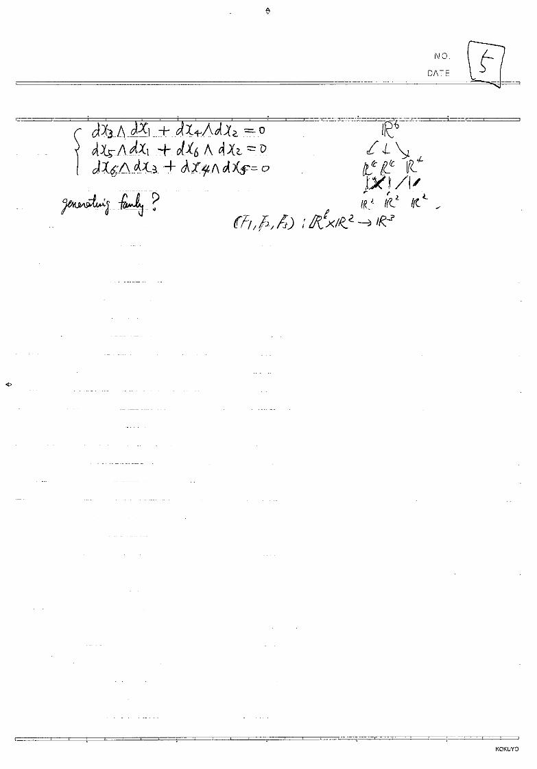
To make the situation clear, we consider R6 with coordinates x1, x2, x3, x4, x5, x6 withthree 2-forms:

ω1 = dx3 ∧ dx1 + dx4 ∧ dx2,

ω2 = dx5 ∧ dx1 + dx6 ∧ dx2,

ω3 = dx6 ∧ dx3 + dx4 ∧ dx5.

Let us consider an integral surface of the differential system ω1 = ω2 = ω3 = 0 whichprojects to (x1, x2) regularly. Then, from ω1 = ω2 = 0, it is written locally

x3 =∂f

∂x1, x4 =

∂f

∂x2, x5 =

∂g

∂x1, x6 =

∂g

∂x2

for some functions f = f(x1, x2), g = g(x1, x2). Then from ω3 = 0, we have the secondorder bilinear partial differential equation on f = f(x1, x2), g = g(x1, x2),

∂2f

∂x21

∂2g

∂x22

+∂2f

∂x22

∂2g

∂x21

− 2∂2f

∂x1∂x2

∂2g

∂x1∂x2= 0.

This equation is regarded as an orthogonality condition of Lagrange-Gauss mapping oftwo Lagrange immersions defined by f and g.

22

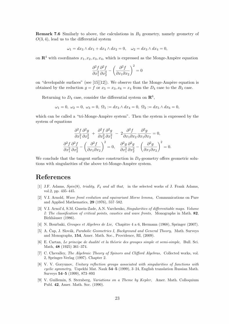
Remark 7.6 Similarly to above, the calculations in B3 geometry, namely geometry ofO(3, 4), lead us to the differential system

ω1 = dx3 ∧ dx1 + dx4 ∧ dx2 = 0, ω2 = dx3 ∧ dx4 = 0,

on R4 with coordinates x1, x2, x3, x4, which is expressed as the Monge-Ampere equation

∂2f

∂x21

∂2f

∂x22

−(

∂2f

∂x1∂x2

)2

= 0

on “developable surfaces” (see [15][12]). We observe that the Monge-Ampere equation isobtained by the reduction g = f or x5 = x3, x6 = x4 from the D4 case to the B3 case.

Returning to D4 case, consider the differential system on R6,

ω1 = 0, ω2 = 0, ω3 = 0, Ω1 := dx3 ∧ dx4 = 0, Ω2 := dx5 ∧ dx6 = 0,

which can be called a “tri-Monge-Ampere system”. Then the system is expressed by thesystem of equations

∂2f

∂x21

∂2g

∂x22

+∂2f

∂x22

∂2g

∂x21

− 2∂2f

∂x1∂x2

∂2g

∂x1∂x2= 0,

∂2f

∂x21

∂2f

∂x22

−(

∂2f

∂x1∂x2

)2

= 0,∂2g

∂x21

∂2g

∂x22

−(

∂2g

∂x1∂x2

)2

= 0.

We conclude that the tangent surface construction in D4-geometry offers geometric solu-tions with singularities of the above tri-Monge-Ampere system.

References

[1] J.F. Adams, Spin(8), triality, F4 and all that, in the selected works of J. Frank Adams,vol.2, pp. 435–445.

[2] V.I. Arnold, Wave front evolution and equivariant Morse lemma, Communications on Pureand Applied Mathematics, 29 (1976), 557–582.

[3] V.I. Arnol’d, S.M. Gusein-Zade, A.N. Varchenko, Singularities of differentiable maps. VolumeI: The classification of critical points, caustics and wave fronts, Monographs in Math. 82,Birkhauser (1986).

[4] N. Bourbaki, Groupes et Algebres de Lie, Chapitre 4 a 6, Hermann (1968), Springer (2007).

[5] A. Cap, J. Slovak, Parabolic Geometries I, Background and General Theory, Math. Surveysand Monographs, 154, Amer. Math. Soc., Providence, RI, (2009).

[6] E. Cartan, Le principe de dualite et la theorie des groupes simple et semi-simple, Bull. Sci.Math, 48 (1925) 361–374.

[7] C. Chevalley, The Algebraic Theory of Spinors and Clifford Algebras, Collected works, vol.2, Springer-Verlag (1997). Chapter 2.

[8] V. V. Goryunov, Unitary reflection groups associated with singularities of functions withcyclic symmetry, Uspekhi Mat. Nauk 54–5 (1999), 3–24, English translation Russian Math.Surveys 54–5 (1999), 873–893

[9] V. Guillemin, S. Sternberg, Variations on a Theme by Kepler, Amer. Math. ColloquiumPubl. 42, Amer. Math. Soc. (1990).

23

[10] S. Helgason, Differential geometry, Lie groups, and Symmetric spaces, Pure and AppliedMath., 80, Academic Press, Inc. New York-London, (1978).

[11] G. Ishikawa, Singularities of tangent varieties to curves and surfaces, Journal of Singularities,6 (2012), 54–83.

[12] G. Ishikawa, Y. Machida, Singularities of improper affine spheres and surfaces of constantGaussian curvature, Intern. J. of Math., 17–3 (2006), 269–293.

[13] G. Ishikawa, Y. Machida, M. Takahashi, Asymmetry in singularities of tangent surfaces incontact-cone Legendre-null duality, Journal of Singularities, 3 (2011), 126–143.

[14] G. Ishikawa, Y. Machida, M. Takahashi, Singularities of tangent surfaces in Cartan’s split G2-geometry, Hokkaido University Preprint Series in Mathematics #1020, (2012). (submitted).

[15] G. Ishikawa, T. Morimoto, Solution surfaces of the Monge-Ampere equation, Diff. Geom. itsAppl., 14 (2001), 113–124.

[16] B. Kostant, The principle of triality and a distinguished unitary representation of SO(4, 4),Differential geometrical methods in theoretical physics (Como, 1987), 65–108, NATO Adv.Sci. Inst. Ser. C Math. Phys. Sci., 250, Kluwer Acad. Publ., Dordrecht, 1988.

[17] M. Mikosz, A. Weber, Triality in so(4, 4), characteristic classes, D4 and G2 singularities,preprint (December 2013). http://www.mimuw.edu.pl/~aweber/publ.html

[18] I.R. Porteous, Clifford Algebras and the Classical Groups, Cambridge Studies in Adv. Math.,50, Cambridge Univ. Press (1995).

[19] T.A. Springer, F.D. Veldkamp, Octonion, Jordan Algebras and Exceptional Groups, Springer-Verlag (2000), Chapter 3.

[20] E. Study, Grundlagen und Ziele der analytischen Kinematik, Sitzungsberichte der BerlinerMathematischen Gesellschaft, 12 (1913), 36–60.

[21] J. Tits, Les groupes de Lie exceptionnels et leur interpretation geometrique, Bull. Soc. Math.Belg. 8 (1956), 48–81.

[22] J. Tits, Sur la trialite et certains groups qui s’en deduisent, I.H.E.S Publ. Math. 2 (1959),13–60.

[23] K. Yamaguchi, Differential systems associated with simple graded Lie algebras, Progress inDifferential Geometry, Advanced Studies in Pure Math., 22 (1993), pp. 413–494.

Goo ISHIKAWA,Department of Mathematics, Hokkaido University, Sapporo 060-0810, Japan.e-mail : ishikawa@math.sci.hokudai.ac.jp

Yoshinori MACHIDA,Numazu College of Technology, Shizuoka 410-8501, Japan.e-mail : machida@numazu-ct.ac.jp

Masatomo TAKAHASHI,Muroran Institute of Technology, Muroran 050-8585, Japan.e-mail : masatomo@mmm.muroran-it.ac.jp

24