MARTINGALE -LIKE BEHAVIOR OF PRICES AND INTEREST RATES

by

Christopher A. Sims

Copyright 1990 by Christopher A. Sims. This paper may be freely reproduced foreducational and research purposes so long as its content is not changed, thiscopyright notice is included in all copies, and the copies are not sold, even tocover costs. This research was supported by NSF grants SES 8309239 and SES 8112026.This paper is an extensive revision of an earlier one with the same title whichappeared as a National Bureau of Economic Research discussion paper in 1980. Thispaper has had more than its share of referees, and though most of them will be happyto be absolved of blame for what is in the paper, the paper is certainly older andwiser for their efforts.

Price changes for a durable good with small storage costs must, in a frictionless

competitive market, be in some sense unpredictable -- or so it seems intuitively.

After all, if the good were reliably predicted to rise very rapidly in price, one

would think the current price should be bid up by speculators eager to cash in on the

predicted capital gains, while if it were reliably predicted to fall rapidly in price

owners of the good would sell their holdings to avoid the predicted capital losses.

These market reactions to predicted price rises or falls should prevent the

occurrence of reliably predicted rises or falls. This intuitive idea has sometimes

been formalized as the hypothesis that the price P of such a good should be atmartingale relative to information observable by market participants, i.e. that, if

X is data which becomes available at t,tp

# p $E P p X , u≤t = P , (1)3 t+sp u 4 t

for any s > 0.

But careful examination of competitive general equilibrium models of behavior under

uncertainty shows, as emphasized by R.E. Lucas, Jr. (1978) and by Stephen F. Leroy

(1973), among others, that (1) emerges from such models only under extremely

restrictive assumptions. The strategy which empirical researchers have sometimes

employed -- testing (1) as an econometric specification to obtain evidence on

whether a market is functioning as a frictionless competitive market -- is therefore

called in to question.

The discrediting of the martingale hypothesis leaves two issues open. Is it then

sheer happenstance that econometric tests of (1) often show it to be close to

correct? And is the intuitive notion that speculators should eliminate predictable

price changes simply fallacious?

This paper puts forward a definition of short-run martingale-like behavior for a

stochastic process. Existing continuous time theoretical models of asset prices make

them satisfy the definition, and this paper shows that under fairly general

assumptions durable goods prices and interest rates will in a frictionless

competitive market show such approximate martingale behavior. More precisely, what is

shown is that the linear regression of P -P on X and lagged X ’s, predicted byt+s t t t

1

2 2(1) to yield an R of zero, instead has an R converging to zero as s goes to

zero. Instead of price changes being unpredictable, price changes over small1intervals are very nearly unpredictable.

Thus if one wishes to interpret an econometric test of (1) as a test of the

importance of frictions and noncompetitive elements in a market, one ought to carry

out the test with s "small". Also, the fact that a price is set in a competitive

market with few frictions and seems to fit (1) reasonably well for, say, an s of

one week, does not mean that (1) should be expected to work well also for an s of

one year.

Two central regularity conditions are required to guarantee the result. One is that

the price stochastic process have what we define below to be "smooth prospects",

meaning that the expected future path of price from t onward is absolutely continuous

on the right at t. We show that if this condition fails simple trading schemes can

achieve unbounded profits. The other condition is that information "flow steadily"

in the sense defined below. Both of these conditions could in principle be violated

in continuous time general equilibrium models, and the paper begins with two examples

where they fail, to give some insight into how "irregular" an economy or an asset

would have to be for these regularity conditions to fail.

The mathematical apparatus of the more abstract part of this paper is similar to that

in some literature on the theory of asset markets in continuous time (such as

Harrison and Kreps (1979), Ross(1978), Huang (1982),and Duffie(1983)). However, that

literature is concerned with deriving conditions on pricing rules from assumptions on

behavior of traders when the number of available securities is limited. In this

paper we assume the existence of a pricing rule which creates no incentive to open

1In the theory of continuous-time stochastic processes, there is a French term

"previsible" which names the property that a stochastic process’s value at t can be

known with arbitrarily high precision at t-s if s is taken small enough. This term

is sometimes translated literally as "previsible" in English-language work on the

subject (as in, e.g., Williams (1979)) but sometimes instead as "predictable." We

will not use "predictable" and "unpredictable" to mean "previsible" and its opposite.

We use the terms sometimes informally as in the footnoted paragraph, and sometimes in

a precise sense in the phrase "instantaneously unpredictable" defined below.2

markets in certain kinds of contingent claims, or equivalently that a rich array of

contingent claims are marketed and arbitrage opportunities do not exist.

Furthermore, we make certain existence and continuity assumptions directly -- the

discount factor for claims to dollars exists and has certain smoothness properties;

prices do change -- without deriving them from maximizing behavior.

In effect, we assume that a competitive market equilibrium exists and has "realistic"

characteristics. From these assumptions we derive the conclusion of approximate

martingale behavior. The harder problem of deriving existence of equilibrium with

realistic price behavior from assumptions about individual behavior is sidestepped.

To follow the argument in detail, the reader will have to be familiar with the theory

of measure and integration on general spaces. I try, however, to illustrate the main

definitions and conclusions with examples, so a reader can grasp what is being

asserted without following the argument in detail.

1. Approximate Martingale Behavior: Instantaneous Unpredictability

The approximate martingale property we will show to hold for durable good prices

might naturally be called the local martingale property -- except that the term

"local martingale" already has a different technical meaning in the theory of

stochastic processes. We will call it instead the property of being "instantaneously

unpredictable."

Definition : A process P(t) is instantaneously unpredictable, or IU at t, if and

only if#& *2$E P( t +v) -E P(t+v)37 8 4t t 2--------------------------------------------------------------------------------------------------------------- [-----L 1 a.s. as v[-----L 0 . (2)

#& *2$E P( t+v ) -P(t)37 8 4t

2Implicit in this definition is that a process does not have the IU property if the

conditional expectations in the definition do not exist a.s. Since asset price

processes might well have infinite first or second moments, this is unsatisfactory.

We could avoid assuming finite moments by working with "local" instantaneous

unpredictability, using "local" in the technical sense of that word in martingale3

In words, for an instantaneously unpredictable process prediction error is the

dominant component of changes over small intervals. Of course, for a martingale with

finite second moments, the ratio in (2) is exactly 1.

Notice that an instantaneously unpredictable process P has the property that thetregression of P -P on any variable observable at t (that is, any variablet+s t 2measurable with respect toF ) has R approaching zero as s goes to zero. Intthis sense, econometric tests of the martingale hypothesis should show the hypothesis

close to true for small s when P is instantaneously unpredictable. The martingalethypothesis, equation (1), will not be exactly true, however, and thus might be

rejected by statistical tests even though the regression of price change on2observable data has very low R .

It might appear that for an instantaneously unpredictable process the chance of (1)

being rejected at standard significance levels is smaller for smaller values of s.

This is not necessarily so, however, because sample size is likely to be related

systematically to s . One plausible situation is that in which there is data

available for a fixed historical time span and we test (1) with s equal one month

using monthly data and (1) with s equal to one week using weekly data, etc. In

this case sample size is inversely proportional to the time interval at which data

are measured. For many plausible models of asset prices -- e.g. diffusion processes2-- the R of a regression of P -P on information available at t goes to zerot+s t

linearly in s . Since the F statistic for the significance of the regression2increases linearly in sample size for a given R , this case of sample size inversely

proportional to s would imply anF statistic tending neither to zero nor infinity as

s decreases to zero. Thus there would be no tendency for fine-time-unit data to

reject the martingale null hypothesis more often.

On the other hand, it is probably true that researchers are likely to undertake tests

of (1) with shorter historical spans of data when they can find data at fine time

units, since there will appear to be so many more degrees of freedom in a given

historical span when data are available at fine time units. Thus one might expect to

theory (see Jacod [], p.6). However it seems better first to present the main ideas

in this less general framework.4

find, in examining existing empirical work for a given type of asset price, that

studies using fine time unit data do reject (1) less often than studies using

coarser time units.

It may help the reader’s understanding of instantaneous unpredictability to consider

some examples. All these examples will focus on the case whereF is simply thetsigma field generated by past values of the price process P itself -- i.e, wheretthe observable information consists only of past and current values of P .t

Any process whose paths with probability one have nicely behaved derivatives fails to

be instantaneously unpredictable. To see this, observe that⋅P -P = vP ,t+v t t+w

where the "." over P indicates time differentiation, for some w

between 0 and v. Forecasting P as of date t, we could uset+v⋅P + vP ,t t

and the resulting expected squared error would certainly be no smaller than that of

the minimum variance forecast, E P . Thus we can be sure thatt t+v# 2$ # ⋅ 2$ # 2 2$E (P -E P ) ≤ E (P -P -vP ) =E v (P -P ) .t3 t+v t t+v 4 t3 t+v t t 4 t3 t+w t 4

But then expression (2) is less than# 2 ⋅ ⋅ 2$ # ⋅ ⋅ 2$E v (P -P ) E ( P - P )t3 t+w t 4 t3 t +w t 4

---------------------------------------------------------------------------------- = -------------------------------------------------------------------------- .2 ⋅ 2v E P ⋅ 2t t E Pt t +w

⋅ ⋅3If the P process is nicely continuous , then at points where P is nonzero, thist texpression converges to zero, not one, as v goes to zero. A verbal paraphrase of

what we have just argued is that, for a differentiable P , the first-order Taylortexpansion in t must provide a forecasting formula whose accuracy becomes high at

small time intervals, in the sense that forecast error from using the formula becomes

small relative to the change predicted by the formula. But our local

unpredictability property (2) is the opposite of this -- an instantaneously

3Mean square continuity is not quite enough. A sufficient condition would be⋅ ⋅ 2E[max (P -P ) ] converging to zero with w.v<w t+v t

5

unpredictable P has forecast error growing large relative to predicted change eventfor the best possible prediction formula.

Any P which is generated by a univariate first-order linear stochastic differentialtequation is instantaneously unpredictable. Suppose it is generated by

⋅P = -aP + u ,t t t4where u is a continuous-time white noise (derivative of a Wiener process). Wet

can verify (2) by notingv-av i -asP = P e + e u dst+v t j t+v-s

0-avE P = P e .t t+v t

Substituting the expressions above into (2) gives usv

#&i -as *2$E e u ds -2avt37j t+v-s 8 4 1-e----------------------------------0 2a

------------------------------------------------------------------------------------------------------------------------------------------------------------ = -------------------------------------------------------------------------------------------------v -2av#& -av i -as *2$ 1-e 2& -av*2E P (1-e )+ e u ds --------------------------------- + P 1-et37 t j t+v-s 8 4 2a t7 8

02Because the second term in the denominator of this expression is 0(v ), while the

term common to numerator and denominator is 0(v), the expression as a whole converges

to one as v goes to zero. It is easy to see that this argument generalizes to the

case of any first-order stochastic differential equation of the formdP = s(P )u + m(P )dt , (3)t t t t

when s(P ) is non-zero and differentiable and m is continuous. Since much work intmodern finance theory begins by assuming that asset prices are diffusion processes,

such work implicitly assumes the local unpredictability property.

Multivariate diffusions can have components which satisfy local unpredictability

almost nowhere. This is obvious when one recalls that a process satisfying a

4Fastidious readers may dislike the practice, common in econometric and engineering

literature, of writing "stochastic differential equations" with driving random terms

without sample paths. They should reinterpret the previous equation to mean that P is2a stationary Gaussian process with spectral density 1/iω+a , where ω is frequency,

or equivalently as asserting that P is stationary with stochastic differential

dP(t)=-aP(t)+dW(t), where W is a Wiener process.6

univariate second-order stochastic differential equation, which will ordinarily have

a continuous derivative process, can be written as one component of a two-dimensional

first-order stochastic differential equation, e.g.dP = Qt t . (4)dQ = - aQ + ut t t

The instantaneous predictability arises because the multivariate analog of s(P ) int(3) is a singular matrix.

Consider a covariance-stationary, linearly regular process (in the terminology of

Rozanov (1967)) with moving average representation P =a*u , where "*" indicatest t5convolution. If P is linear, so that best linear prediction coincides with

conditional expectation, then P is instantaneously unpredictable if a has a right-slimit at s=0 which is non-zero, and is nowhere instantaneously unpredictable if it

has a right-limit at zero which is zero.

1. The Flow of Information

We begin by specifying a spaceΩ of states of the world z and a setF of events,

subsets ofΩ. F is supposed closed under the taking of complements and countable

unions and to contain the null set, makingF a sigma-field. The flow of

information is described by the collection F , where each F is a sub-sigmat tfield of F and consists of the events which are verifiable at t -- that is, if

an event is in F , at dates t and later we know whether the event occurred. Wetassume that an event verifiable at t is also verifiable later, i.e. that F istincreasing, or F includes F for all t > s .t s

The sequence F describes the way information increases over time. The setuptoften used in macroeconomic theorizing, where information available at t is taken

to be current and past values of some vector of real variables X , can betaccommodated as a special case of this more general specification. The X vector ist

5Here again fastidious readers might prefer that we be explicit: P(t)=a*u , with utthe derivative of the Wiener process W, means that P and W are jointly Gaussian with

s& * i icov P(t),W(s) = a(t-v)dv for any t,s, or equivalently that P(t) = a(t-v)W(dv) .7 8 j j

-∞7

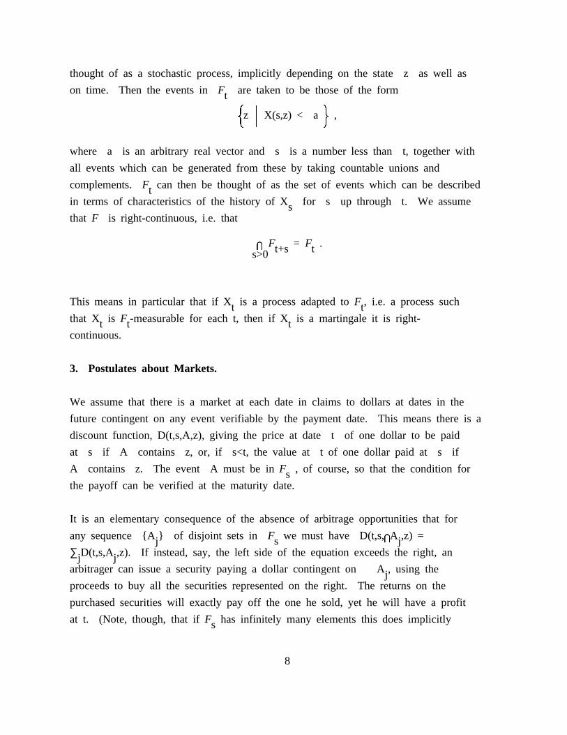
thought of as a stochastic process, implicitly depending on the state z as well as

on time. Then the events inF are taken to be those of the formt( )

2z X(s,z) < a ,

29 0

where a is an arbitrary real vector and s is a number less than t, together with

all events which can be generated from these by taking countable unions and

complements. F can then be thought of as the set of events which can be describedtin terms of characteristics of the history of X for s up through t. We assumesthat F is right-continuous, i.e. that

n F = F .t+s ts>0

This means in particular that if X is a process adapted toF , i.e. a process sucht tthat X is F -measurable for each t, then if X is a martingale it is right-t t tcontinuous.

3. Postulates about Markets.

We assume that there is a market at each date in claims to dollars at dates in the

future contingent on any event verifiable by the payment date. This means there is a

discount function, D(t,s,A,z), giving the price at date t of one dollar to be paid

at s if A contains z, or, if s<t, the value at t of one dollar paid at s if

A contains z. The event A must be inF , of course, so that the condition forsthe payoff can be verified at the maturity date.

It is an elementary consequence of the absence of arbitrage opportunities that for

any sequence A of disjoint sets inF we must have D(t,s,nA ,z) =j s j∑ D(t,s,A ,z). If instead, say, the left side of the equation exceeds the right, anj jarbitrager can issue a security paying a dollar contingent on A , using thejproceeds to buy all the securities represented on the right. The returns on the

purchased securities will exactly pay off the one he sold, yet he will have a profit

at t. (Note, though, that ifF has infinitely many elements this does implicitlys

8

assume that infinite collections of contingent securities exist and can be bought and

sold.)

It is also reasonable to suppose that D is always finite. We assume there is a

probability measure m defined onF and hence also a restriction of m, called

m , to F for each t. Think of m as being the "market" probability measure ont tstates of the world. We require that if m(A)=0, D(t,s,A,z)=0 for all t,z. That is,

claims to a dollar contingent on events of "market" probability zero are valueless.

While these conditions would hold if m were the "true" probability measure and agents

were rational in the sense that they put value zero on securities which pay off only

under conditions with probability zero, there is no requirement that m represent

truth. The probability statements we will derive take m as the underlying

distribution, but any m which puts probability zero only on sets which the market

also gives probability zero will do. Thus if we use a "false" econometric model, it

will still show the properties we derive in what follows, so long as the econometric

model does not rule out as impossible events the market treats as possible.

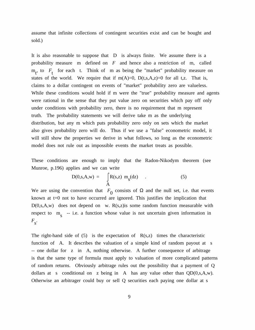
These conditions are enough to imply that the Radon-Nikodym theorem (see

Munroe, p.196) applies and we can writeiD(0,s,A,w) = R(s,z) m (dz) . (5)j sA

We are using the convention thatF consists ofΩ and the null set, i.e. that events0known at t=0 not to have occurred are ignored. This justifies the implication that

D(0,s,A,w) does not depend on w. R(s,z)is some random function measurable with

respect to m -- i.e. a function whose value is not uncertain given information insF .s

The right-hand side of (5) is the expectation of R(s,z) times the characteristic

function of A. It describes the valuation of a simple kind of random payout at s

-- one dollar for z in A, nothing otherwise. A further consequence of arbitrage

is that the same type of formula must apply to valuation of more complicated patterns

of random returns. Obviously arbitrage rules out the possibility that a payment of Q

dollars at s conditional on z being in A has any value other than QD(0,s,A,w).

Otherwise an arbitrager could buy or sell Q securities each paying one dollar at s

9

contingent on A, while selling or buying one security paying Q dollars at s

contingent on A, making a profit.

This, together with our other assumptions, gives us a formula for valuing random

payouts which pay Q dollars if z is in A , i=1,...,k, where the sets A arei i idisjoint. Call this a "simple payout pattern." Suppose a security paying H(z) at s

has the property that we can bound H(z) above and below by linear combinations of

characteristic functions of finite collections of disjoint sets. Arbitrage should

preclude the security from being valued outside the range given by the values of

securities with simple payout patterns which bound H. This is enough to guarantee

that securities with random payouts will be valued as integrals of their payouts if

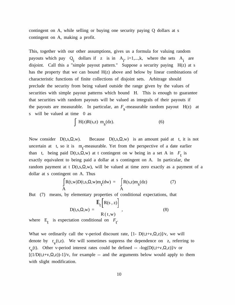
the payouts are measurable. In particular, anF -measurable random payout H(z) atss will be valued at time 0 as

i H(z)R(s,z) m (dz). (6)j s

Now consider D(t,s,Ω,w). Because D(t,s,Ω,w) is an amount paid at t, it is not

uncertain at t, so it is m -measurable. Yet from the perspective of a date earliertthan t, being paid D(t,s,Ω,w) at t contingent on w being in a set A inF istexactly equivalent to being paid a dollar at s contingent on A. In particular, the

random payment at t D(t,s,Ω,w), will be valued at time zero exactly as a payment of a

dollar at s contingent on A. Thusi iR(t,w)D(t,s,Ω,w)m (dw) = R(s,z)m (dz) (7)j t j sA A

But (7) means, by elementary properties of conditional expectations, that# $E R(s , z)t3 4

D(t,s,Ω,w) = -------------------------------------------------- , (8)R ( t ,w)

where E is expectation conditional onF .t t

What we ordinarily call the v-period discount rate, [1- D(t,t+v,Ω,z)]/v, we will

denote by r (t,z). We will sometimes suppress the dependence on z, referring tovr (t). Other v-period interest rates could be defined -- -log(D(t,t+v,Ω,z)]/v orv[(1/D(t,t+v,Ω,z))-1]/v, for example -- and the arguments below would apply to them

with slight modification.

10

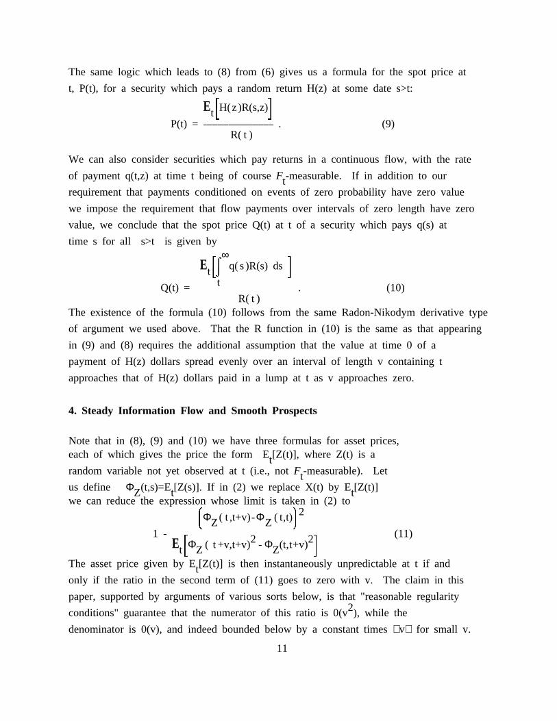
The same logic which leads to (8) from (6) gives us a formula for the spot price at

t, P(t), for a security which pays a random return H(z) at some date s>t:# $E H(z)R(s,z)t3 4

P(t) = ----------------------------------------------------------------- . (9)R( t )

We can also consider securities which pay returns in a continuous flow, with the rate

of payment q(t,z) at time t being of courseF -measurable. If in addition to ourtrequirement that payments conditioned on events of zero probability have zero value

we impose the requirement that flow payments over intervals of zero length have zero

value, we conclude that the spot price Q(t) at t of a security which pays q(s) at

time s for all s>t is given by∞

#i $E q( s )R(s) dst3j 4tQ(t) = -------------------------------------------------------------------------------------- . (10)

R( t )The existence of the formula (10) follows from the same Radon-Nikodym derivative type

of argument we used above. That the R function in (10) is the same as that appearing

in (9) and (8) requires the additional assumption that the value at time 0 of a

payment of H(z) dollars spread evenly over an interval of length v containing t

approaches that of H(z) dollars paid in a lump at t as v approaches zero.

4. Steady Information Flow and Smooth Prospects

Note that in (8), (9) and (10) we have three formulas for asset prices,each of which gives the price the form E [Z(t)], where Z(t) is atrandom variable not yet observed at t (i.e., notF -measurable). Lettus define Φ (t,s)=E [Z(s)]. If in (2) we replace X(t) by E [Z(t)]Z t twe can reduce the expression whose limit is taken in (2) to

& *2Φ ( t ,t+v)-Φ ( t,t)7 Z Z 8

1 - --------------------------------------------------------------------------------------------------------------------------------------- (11)# 2 2$E Φ ( t +v,t+v) - Φ (t,t+v)t3 Z Z 4

The asset price given by E [Z(t)] is then instantaneously unpredictable at t if andtonly if the ratio in the second term of (11) goes to zero with v. The claim in this

paper, supported by arguments of various sorts below, is that "reasonable regularity2conditions" guarantee that the numerator of this ratio is 0(v ), while the

denominator is 0(v), and indeed bounded below by a constant timesv for small v.

11

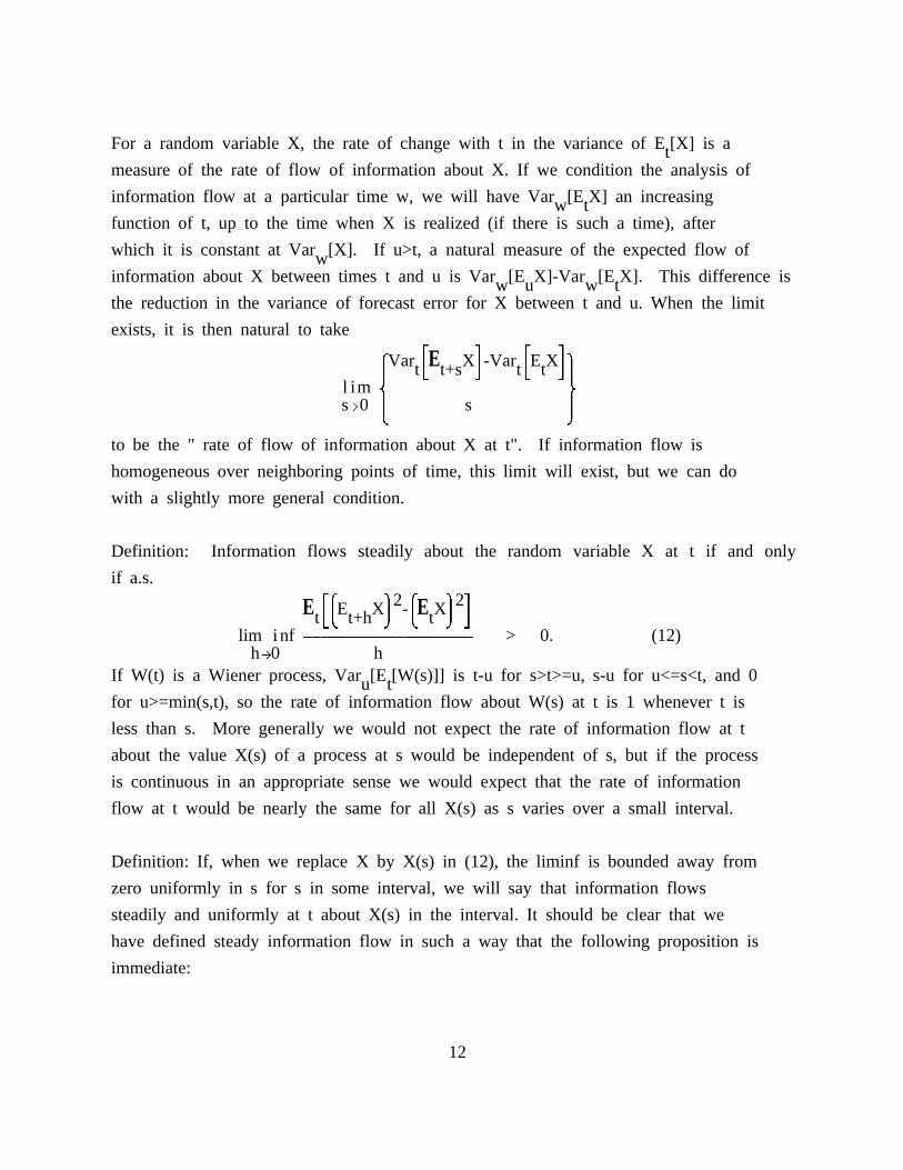
For a random variable X, the rate of change with t in the variance of E [X] is atmeasure of the rate of flow of information about X. If we condition the analysis of

information flow at a particular time w, we will have Var [E X] an increasingw tfunction of t, up to the time when X is realized (if there is such a time), after

which it is constant at Var [X]. If u>t, a natural measure of the expected flow ofwinformation about X between times t and u is Var [E X]-Var [E X]. This difference isw u w tthe reduction in the variance of forecast error for X between t and u. When the limit

exists, it is then natural to take( # $ # $)Var E X -Var E X2 t3 t+s 4 t3 t 42

l im ------------------------------------------------------------------------------------------------------sL0 2 s 2

9 0

to be the " rate of flow of information about X at t". If information flow is

homogeneous over neighboring points of time, this limit will exist, but we can do

with a slightly more general condition.

Definition: Information flows steadily about the random variable X at t if and only

if a.s.#& *2 & *2$E E X - E Xt37 t+h 8 7 t 8 4

lim inf ------------------------------------------------------------------------------------------------- > 0. (12)hL0 h

If W(t) is a Wiener process, Var [E [W(s)]] is t-u for s>t>=u, s-u for u<=s<t, and 0u tfor u>=min(s,t), so the rate of information flow about W(s) at t is 1 whenever t is

less than s. More generally we would not expect the rate of information flow at t

about the value X(s) of a process at s would be independent of s, but if the process

is continuous in an appropriate sense we would expect that the rate of information

flow at t would be nearly the same for all X(s) as s varies over a small interval.

Definition: If, when we replace X by X(s) in (12), the liminf is bounded away from

zero uniformly in s for s in some interval, we will say that information flows

steadily and uniformly at t about X(s) in the interval. It should be clear that we

have defined steady information flow in such a way that the following proposition is

immediate:

12

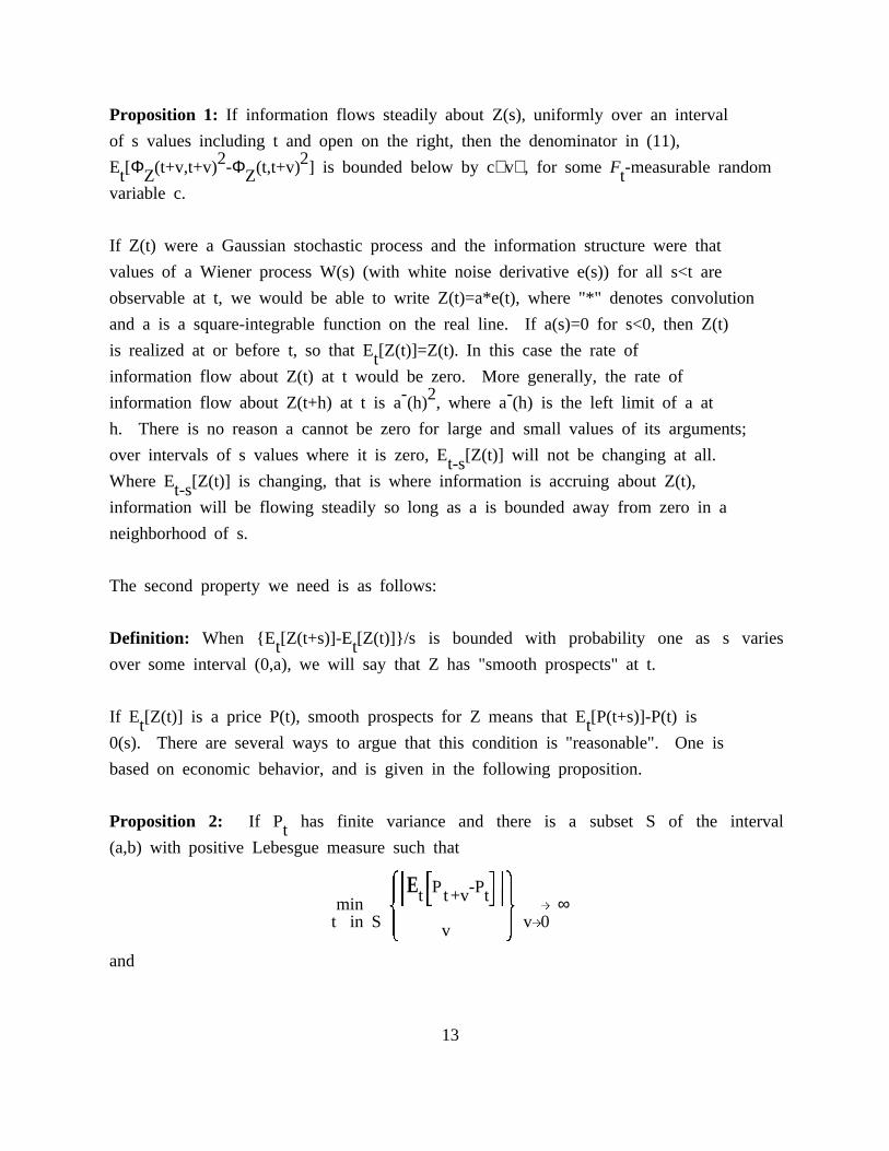
Proposition 1: If information flows steadily about Z(s), uniformly over an interval

of s values including t and open on the right, then the denominator in (11),2 2E [Φ (t+v,t+v) -Φ (t,t+v) ] is bounded below by cv, for someF -measurable randomt Z Z t

variable c.

If Z(t) were a Gaussian stochastic process and the information structure were that

values of a Wiener process W(s) (with white noise derivative e(s)) for all s<t are

observable at t, we would be able to write Z(t)=a*e(t), where "*" denotes convolution

and a is a square-integrable function on the real line. If a(s)=0 for s<0, then Z(t)

is realized at or before t, so that E [Z(t)]=Z(t). In this case the rate oftinformation flow about Z(t) at t would be zero. More generally, the rate of

- 2 -information flow about Z(t+h) at t is a (h) , where a (h) is the left limit of a at

h. There is no reason a cannot be zero for large and small values of its arguments;

over intervals of s values where it is zero, E [Z(t)] will not be changing at all.t-sWhere E [Z(t)] is changing, that is where information is accruing about Z(t),t-sinformation will be flowing steadily so long as a is bounded away from zero in a

neighborhood of s.

The second property we need is as follows:

Definition: When E [Z(t+s)]-E [Z(t)]/s is bounded with probability one as s variest tover some interval (0,a), we will say that Z has "smooth prospects" at t.

If E [Z(t)] is a price P(t), smooth prospects for Z means that E [P(t+s)]-P(t) ist t0(s). There are several ways to argue that this condition is "reasonable". One is

based on economic behavior, and is given in the following proposition.

Proposition 2: If P has finite variance and there is a subset S of the intervalt(a,b) with positive Lebesgue measure such that

( )2 # $2

2 E P -P 22 t3 t+v t42min ----------L ∞---------------------------------------------------------------t in S 2 2 vL0v9 0

and

13

( )& # $*2

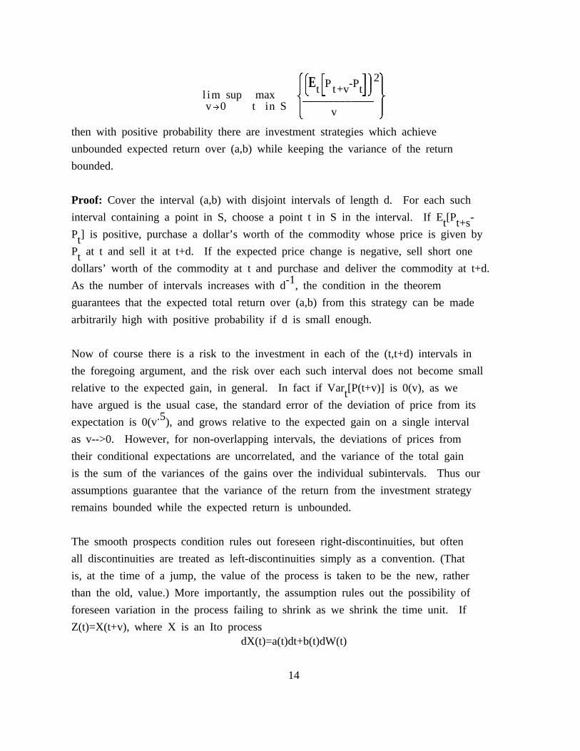
2 E P -P 27 t3 t+v t48l im sup max ---------------------------------------------------------------vL0 t in S 2 2v

9 0

then with positive probability there are investment strategies which achieve

unbounded expected return over (a,b) while keeping the variance of the return

bounded.

Proof: Cover the interval (a,b) with disjoint intervals of length d. For each such

interval containing a point in S, choose a point t in S in the interval. If E [P -t t+sP ] is positive, purchase a dollar’s worth of the commodity whose price is given bytP at t and sell it at t+d. If the expected price change is negative, sell short onetdollars’ worth of the commodity at t and purchase and deliver the commodity at t+d.

-1As the number of intervals increases with d , the condition in the theorem

guarantees that the expected total return over (a,b) from this strategy can be made

arbitrarily high with positive probability if d is small enough.

Now of course there is a risk to the investment in each of the (t,t+d) intervals in

the foregoing argument, and the risk over each such interval does not become small

relative to the expected gain, in general. In fact if Var [P(t+v)] is 0(v), as wethave argued is the usual case, the standard error of the deviation of price from its

.5expectation is 0(v ), and grows relative to the expected gain on a single interval

as v-->0. However, for non-overlapping intervals, the deviations of prices from

their conditional expectations are uncorrelated, and the variance of the total gain

is the sum of the variances of the gains over the individual subintervals. Thus our

assumptions guarantee that the variance of the return from the investment strategy

remains bounded while the expected return is unbounded.

The smooth prospects condition rules out foreseen right-discontinuities, but often

all discontinuities are treated as left-discontinuities simply as a convention. (That

is, at the time of a jump, the value of the process is taken to be the new, rather

than the old, value.) More importantly, the assumption rules out the possibility of

foreseen variation in the process failing to shrink as we shrink the time unit. If

Z(t)=X(t+v), where X is an Ito processdX(t)=a(t)dt+b(t)dW(t)

14

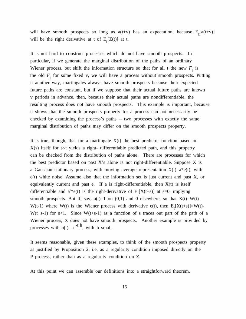
will have smooth prospects so long as a(t+v) has an expectation, because E [a(t+v)]twill be the right derivative at t of E [Z(t)] at t.t

It is not hard to construct processes which do not have smooth prospects. In

particular, if we generate the marginal distribution of the paths of an ordinary

Wiener process, but shift the information structure so that for all t the newF istthe old F for some fixed v, we will have a process without smooth prospects. Puttingtit another way, martingales always have smooth prospects because their expected

future paths are constant, but if we suppose that their actual future paths are known

v periods in advance, then, because their actual paths are nondifferentiable, the

resulting process does not have smooth prospects. This example is important, because

it shows that the smooth prospects property for a process can not necessarily be

checked by examining the process’s paths -- two processes with exactly the same

marginal distribution of paths may differ on the smooth prospects property.

It is true, though, that for a martingale X(t) the best predictor function based on

X(s) itself for s<t yields a right- differentiable predicted path, and this property

can be checked from the distribution of paths alone. There are processes for which

the best predictor based on past X’s alone is not right-differentiable. Suppose X is

a Gaussian stationary process, with moving average representation X(t)=a*e(t), with

e(t) white noise. Assume also that the information set is just current and past X, or

equivalently current and past e. If a is right-differentiable, then X(t) is itself

differentiable and a′*e(t) is the right-derivative of E [X(t+s)] at s=0, implyingtsmooth prospects. But if, say, a(t)=1 on (0,1) and 0 elsewhere, so that X(t)=W(t)-

W(t-1) where W(t) is the Wiener process with derivative e(t), then E [X(t+s)]=W(t)-tW(t+s-1) for s<1. Since W(t+s-1) as a function of s traces out part of the path of a

Wiener process, X does not have smooth prospects. Another example is provided by-t hprocesses with a(t) =e t , with h small.

It seems reasonable, given these examples, to think of the smooth prospects property

as justified by Proposition 2, i.e. as a regularity condition imposed directly on the

P process, rather than as a regularity condition on Z.

At this point we can assemble our definitions into a straightforward theorem.

15

Theorem 1: If P(t) is an asset price which can be written in the form E [Z(t)],twhere Z(t) is a stochastic process such that Z(t) is not realized at t, then if

i) information flows steadily at t about Z(s) uniformly over an interval of s

values including t and open on the right, and

ii) P has smooth prospects at t,

then P is instantaneously unpredictable at t.

Proof: Follows immediately by combining Proposition 1, the definition of smooth

prospects, the definition of instantaneous unpredictability, and the decomposition of

the defining formula for instantaneous unpredictability as given in (11).

Theorem 1 contains the main idea of this paper. However it is limited in two ways

which justify some further discussion. For one, asset price processes do not always

appear to have variances, or even expectations, yet the discussion leading to Theorem

1 is based heavily on the first two moments. This approach allows more elementary

methods to be used, but the same ideas can be extended to produce a "local" result,

in the terminology of modern martingale theory, which is not tied to existence of

moments in the same way. The other limitation is that, though the steady information

flow about Z assumption is reasonable, we cannot discuss the kinds of pathology in an

economic model which might lead to its being violated without going behind Z, to its

numerator (future returns) and denominator (the random discount factor R(t)).

Natural second-moment assumptions about numerator and denominator do not translate

easily into second-moment restrictions on Z, because Z is a nonlinear function of

numerator and denominator. To explore the mapping between regularity conditions on

the joint behavior of numerator and denominator of Z and regularity conditions on Z

itself, we need to apply Ito’s formula, the central tool of stochastic calculus.

For each of the cases we have considered, the expected returns component of Z in the

numerator is very naturally taken to have smooth prospects and to have smooth

information flow concerning it. The R(t) denominator for Z, however, is almost

unrestricted by the arbitrage theory. We will first examine how pathological

behavior of R might arise and how it might affect our results under some assumptions

16

which make use of Ito’s formula very convenient and which are very common in the

finance literature, but are in fact rather restrictive.

5. The Case of Information Generated by Finitely Many Wiener Processes.

Information structures can be characterized by the martingales defined on them.

Economic theoretical models are likely most often to be constructed under the

convenient assumption that finitely many Wiener processes generate the information

structure. A common assumption in theoretical models is that all processes in the

model are Ito processes relative to a finite information vector of Wiener processes,

meaning that any process X has differentialdX(t) = a(t)dt + b(t)dW(t) ,

where a(t) is a scalar process and b(t) a vector process, both adapted to F . W(t)tis a vector of mutually orthogonal Wiener processes.

For such an X, it is easy to check that X is instantaneously unpredictable at t if

b(t) is non-zero almost surely, because the smooth prospects property is implicit in

the form of dX(t) -- (d/dv)E [X(t+v)] at v=0 is just a(t).t

Each of the pricing formulas (8)-(10) has the formH(t)P(t) = ----------------- ,R(t)

where H(t) is expected discounted returns from t onward and R is the random

discount factor. These components, under our current regularity assumptions, will

be taken to have the form

dH(t) = a (t) dt + b (t) dWH H ,

dR(t) = a (t) dt + b (t) dWR Rwhere a , a , b , and b are all stochastic processes and, by Ito’s formula,R H R H

# $ # $H 1 H 1 HdP(t) = 2- -------------a - ------------b b ′ +.5-------------b b ′ 2dt + 2-------b - -------------b 2dW(t) .2 R 2 H R 3 R R H 2 R3 R R R 4 3R R 4

So P will be instantaneously unpredictable unless b =Pb a.s. Because the H process isH Rthe conditional expectation of future returns and future returns as of t are not

observed at t, it is natural that b is non-zero -- otherwise information would notHbe flowing about future returns at t. If b is non-zero, we are then assured that PRis IU.

17

More generally, we will have b non-zero. If b =Pb , and both are nonzero, then HR H Rand R are both being driven by the same one-dimensional martingale with differential

b dW. If the equality held a.s. for every t, it would imply that short run changesRin R and H are perfectly correlated. Unless the returns H and the discount factor R

are jointly singular in this sense, it will not be possible to avoid instantaneous

unpredictability in P.

Consider the case where H(t)=E [R(T)] and P(t) is therefore the discount factor fortterm T-t. Though in this case H(t) and R(t) both come from the R process in some

sense, it is still unlikely that b^H^ and b are linearly dependent. If they wereRlinearly dependent for every t and T, the implication would be that prediction of R

can be based on a one-dimensional martingale rather than requiring use of all the

elements of the W vector individually.

It may help the reader’s intuition to consider the special case where log R and log H

are jointly Gaussian processes. This means thatdlog H = a (t) dt + b (t) dW(t) andH H

dlog R = a (t) dt + b (t) dW(t)R Rwith a and a Gaussian processes and b , and b deterministic, though time-R H R Hvarying, vectors.

This implies

# 2$ # $dP(t) = a -a +.5@b -b @ P(t)dt + P(t) b -b dW .3 H R H R 4 3 H R4

Instantaneous unpredictability emerges, therefore, unless b =b . As we noted above,H Rb =b amounts to a kind of singularity in the joint distribution of small changes inH RH and R, with the small changes being nearly perfectly correlated. While such a

result might emerge in a model with a single source of stochastic disturbance, more

generally, if there are several kinds of real asset, each with its own random

variations in return, it will be impossible for H and R to show such exact

collinearity for every security.

18

Now assume log R is in addition a process with stationary increments and consider the

case of a discount bill, i.e. H(t)=E [R(T)]. The stationarity gives us that a ist Rstationary and b is a constant. Now if log R has stationary increments, we canRwrite it as

tilog R(t) = log R (t) + c(s) dW(t-s) , (13)0 j0

where c(s) is a vector-valued function square-integrable over finite intervals and R0is a function whose path is known at time 0. From (13) we obtain

log E [R(T)] = log H(t)tT-t Ti i= log R (t) + .5 c(s)c(s)’ ds + c(s) dW(T-s) ds , (14)0 j j0 T- t

where we are using the lognormality of R(T) conditional onF and applying thetm+.5vformula that if log(x) is distributed as N(m,v), then E[x]=e .

Assuming c is differentiable, we obtain from (14)

dlog H(t)

T# ⋅ i $= (R (t)/R (t))-.5c(T-t)c(T-t)′+ c′(s)dW(T-s) dt + c(T-t)dW(t) .(15)3 0 0 j 4

T- tBut this means that c(T-t)=b (t) identically, and since b =b , a constant, in theH H Rcase where instantaneous unpredictability fails, this case entails c(s) being a

constant vector. If c(s) is constant, log R is a deterministic function of time plus

a Wiener process. It is not hard to check that this means that the term structure of

interest rates varies only deterministically with time.

The conclusion is that if log R is a Gaussian process with stationary increments, the

process of discount factors for dollars delivered at a fixed date in the future can

fail to be instantaneously unpredictable only if there is no uncertainty about future

interest rates.

Before proceeding we should reemphasize that in this entire section, by assuming that

R has a nice stochastic differential, we have been ignoring the possibility of R’s

failing to have smooth prospects. We have been exploring only the possibility that,

despite steady information flow about future returns, steady information flow about Z

might fail because variation in R exactly cancels the effects of information flow on19

H(t). Our conclusion is that this seems to occur only with a kind of one-

dimensionality in information flow.

6. Semimartingales, Local Martingales.

The previous section’s discussion of the case where the information structure is

generated by finitely many Wiener processes probably covers the cases most likely to

emerge from theoretical economic models, because such information structures are both

convenient and quite general. It would be disturbing, however, if results depended

strongly on this assumption of convenience. Furthermore, it rules out the possibility

of discontinuities in H(t). There is no reason to suppose it to be impossible for

information to arrive at an instant, causing H(t) to make a discontinuous jump. If

the information structure is generated by a set of continuous martingales, such jumps

are impossible. One might suppose that such jumps could disturb the instantaneous

unpredictability result. It turns out that they can, but only if information about

the size or timing of the jumps flows "non-smoothly" in a certain sense.

To be able to consider information structures in which information arrives

discontinuously as well as continuously, and to sidestep the convenient but ad hoc

assumption that information is generated by finitely many martingales, we need to

introduce some definitions and results following Jacod (1979).

Definition: A "stopping time" is a random variable T with values in the extended real

line (i.e., its values are real numbers or infinity) with the property that the6condition T>t is verifiable at t, i.e. T>t is inF .t

Definition: If T is a stopping time and X a stochastic process adapted toF , wetTdenote by X the stochastic process defined byT TX (t)=X(t) if t<T, X (t)=X(T) If t ≥T.

TX is called "X stopped at T."

6This is Lipster and Shiryaev’s [1977] definition of a "Markov time." They reserve

"stopping time" for an a.s. finite Markov time. To make this definition coincide

with Jacod’s definition of a stopping time, we must assume thatF is generated by a

class of right-continuous processes with left limits.20

Definition: If Q is a property of stochastic processes, we say that the process X

has the property Q "locally" if and only if there is a sequence of stopping timesT(n)T(n) converging to infinity a.s. such that X has property Q for each T(n).

Local martingales are processes which have the martingale property locally in this

sense. Local martingales are important in part because martingales themselves are

defined by moment properties. Certain modifications of martingale processes whose

paths look like those of martingales thus lose the martingale property. For example,

suppose X(t) over the interval [0,3] is a Wiener process with parameter S, that is a

continuous martingale with independent increments and#& *2$ 2E X(t+s)-X(t) = (t-s)S .t37 8 4

If at time t=3 we reset S as1/X(3) and then let X evolve with this new S, we have

generated a process whose paths will just be those of a martingale whose parameter

changes at t=3. But since1/X(3), as the absolute value of the inverse of a normal

random variable, has infinite expectation, E [X ] is not defined as a Lebesguet t+sintegral for t+s>3 and t<3. This process is a local martingale, though: take T(n)

=infinity if X(3)<n, otherwise T(n)=3. This T(n) clearly converges a.s. to infinity,T(n)while X is a martingale for each n.

Note that if X has the property Q locally, and if we have data on a single

realization of X for a finite time span (s,t), we could never find evidence against X

having property Q by examining the data. For any c>0 we can choose a stopped version

of X which does have property Q and whose probability of exactly matching the time

path of X itself over (s,t) exceeds (1-c). Hence the observed path of X always has a

high probability of exactly matching one from a process with property Q.

Definition: A process X is called a "semimartingale" if it can be written in the

form X=M+A, where M is a local martingale and A’s paths have bounded variation.

Semimartingales are in some senses quite general. With the usual approach to

stochastic integration, they are the most general class of processes with respect to

which a stochastic integral is defined. Note, though, that if W is a Wiener process,.2 -tW(t)-W(t-1) is not a semimartingale, and also that if a(t)=te for t>0, 0 for t<0,

then X=a*ε, with ε white noise, is not a semimartingale. Semimartingales are

21

processes such that E [X(t+s)] does not behave outrageously as a function of s. Intboth the foregoing examples E [X(t+s)] is almost surely not right differentiable in stat s=0. These two examples are also examples we gave of processes without smooth

prospects. A semimartingale can fail to have smooth prospects -- for example A can

have jump discontinuities at dates known in advance.

Proposition 2: If X is a semimartingale and if its bounded variation component A can

be chosen to have paths a.s. absolutely continuous with Radon-Nikodym t-derivative at

t, DA(t), existing a.s. at t and a.s. bounded in absolute value in a neighborhood of

t by the F -measurable random variable B(t), then X has smooth prospects.t

Proof: By construction,s

# $ # $ # i $E X(t+s)-X(t) = E A(t+s)-A(t) = E DA(t+v) dv .t3 4 t3 4 t3 j 40

The conclusion then follows directly from the definition of smooth prospects and the

boundedness assumption on DA.

Now consider a vector semimartingale process X which can be writtenc dX = A + M + M , (16)

cwhere M is a local martingale with a.s. continuous paths, A is continuous and ofdbounded variation, and M is a square integrable local martingale with paths of

locally integrable bounded variation, which implies it changes only in discontinuous

jumps. Such a decomposition exists and is unique if X is what Jacod calls a "left

quasicontinuous special semimartingale" and is locally square-integrable.

We wish to impose sufficient regularity on the three components of X that we can

guarantee local smooth prospects for F(X), whereF is a twice-differentiable

function. A generalized version of Ito’s formula (given as Jacod’s (3.89)) allows us

to check the effect of these regularity conditions. We will not attempt to attaindthe greatest possible generality in our result. Doing so with respect to the M

component would raise mathematical difficulties.

Obviously to begin we want to insure that X itself has locally smooth prospects.

22

Condition I: A in (16) has absolutely continuous paths with Radon-Nikodym

derivative a.s. bounded in absolute value in a neighborhood of t by anF -tmeasurable random variable.

Definition: If M is a local martingale with continuous paths, its "quadratic

variation" <M,M> is defined as the unique stochastic process such that MM′-<M,M> is a

local martingale.

Note that M is a column vector and <M,M> a matrix-valued process. <M,M> is increasing

in the sense that <M,M>(t)-<M,M>(s) is positive semidefinite for t>s.

c c cCondition II: M has quadratic variation <M ,M > with Radon-Nikodym derivative V,+bounded above in a neighborhood of t by the random matrix V (t), which isF -t

measurable.

dWe will take M to behave over small intervals after t like a process which takes anjump distributed with probability measure over R (n being the dimension of X) given

by q(t,.) and probability per unit time of a jump h(t). That is, if Q(t,s,.) is thedconditional probability measure for M (t+s) givenF , we requiret

Condition III: D Q(t,t,C+X(t)) = h(t)q(t,C) , for C not containing 0, D Q(t,t,0)=-2 2h(t), with h bounded in a neighborhood of t and q in a neighborhood of t

concentrating probability in a set of jumps of bounded length, both bounds beingF -tmeasurable.

Condition III restricts jumps in X to be "unpredictably timed." While condition III

could be generalized somewhat, jumps occurring at times known in advance undo the

smooth prospects property. Even if H and R each have smooth prospects, if R has a

discontinuous martingale component with jumps at dates known in advance, H/R will not

have smooth prospects. The problem is that even though the jump in R has zero

expectation, it generates a jump in 1/R with nonzero expectation, and this generates

a jump with both size and timing known in advance in the A component of X/R.

c dProposition 4: If X=A+M +M , with the components satisfying conditions I-III, and if

F is a twice-differentiable function, then F(X) locally has smooth prospects.

23

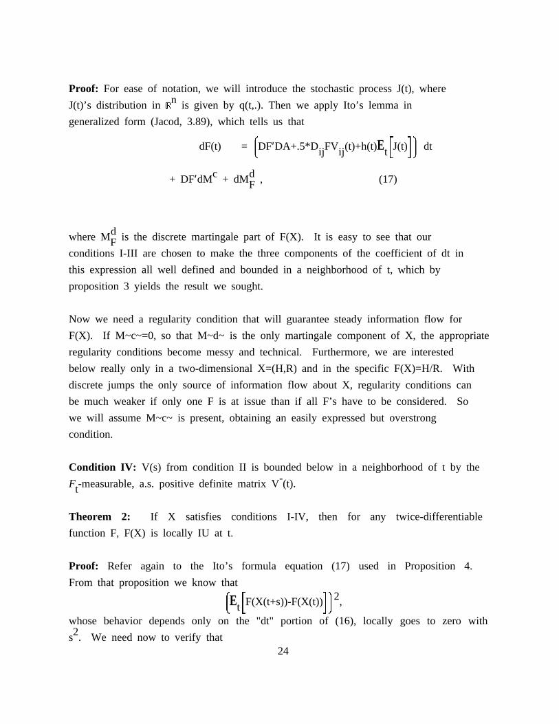
Proof: For ease of notation, we will introduce the stochastic process J(t), wherenJ(t)’s distribution inR is given by q(t,.). Then we apply Ito’s lemma in

generalized form (Jacod, 3.89), which tells us that

& # $*dF(t) = DF′DA+.5*D FV (t)+h(t)E J(t) dt7 ij ij t 3 48

c d+ DF′dM + dM , (17)F

dwhere M is the discrete martingale part of F(X). It is easy to see that ourFconditions I-III are chosen to make the three components of the coefficient of dt in

this expression all well defined and bounded in a neighborhood of t, which by

proposition 3 yields the result we sought.

Now we need a regularity condition that will guarantee steady information flow for

F(X). If M~c~=0, so that M~d~ is the only martingale component of X, the appropriate

regularity conditions become messy and technical. Furthermore, we are interested

below really only in a two-dimensional X=(H,R) and in the specific F(X)=H/R. With

discrete jumps the only source of information flow about X, regularity conditions can

be much weaker if only one F is at issue than if all F’s have to be considered. So

we will assume M~c~ is present, obtaining an easily expressed but overstrong

condition.

Condition IV: V(s) from condition II is bounded below in a neighborhood of t by the-F -measurable, a.s. positive definite matrix V (t).t

Theorem 2: If X satisfies conditions I-IV, then for any twice-differentiable

function F, F(X) is locally IU at t.

Proof: Refer again to the Ito’s formula equation (17) used in Proposition 4.

From that proposition we know that& # $*2E F(X(t+s))-F(X(t)) ,7 t3 48

whose behavior depends only on the "dt" portion of (16), locally goes to zero with2s . We need now to verify that

24

#& *2$E F(X(t+s))-F(X(t)) ,t37 8 4

is locally bounded below by bs for some b>0 for small s. But the "dt" portion of2 c(16) contributes only an 0(s ) term to this expression. The M component of (16)

-contributes an 0(s) term bounded below by cDF(t)′V (t)DF(t)s for small s. The

discrete martingale term contributes a component which may also be 0(s). Might itccancel the contribution of the M component? We know it cannot do so because

square-integrable purely discrete-jump martingales must be locally uncorrelated with

purely continuous-path martingales (Jacod, (2.27a)), which completes the proof.

Corollary: If the bivariate process (H,R) satisfies I-IV, and if R is locally a.s.

bounded away from zero on an interval (t,t+s), with s>0, by a positiveF -measurabletrandom variable, then the asset price H/R is locally IU at t.

Proof: Just an application of the theorem. The bound on R is needed to ensure that

H/R is twice-differentiable over the relevant range.

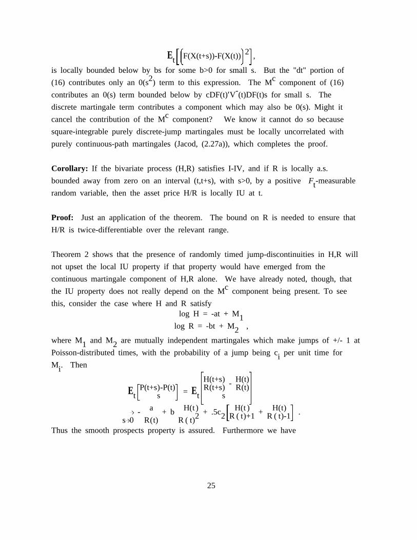
Theorem 2 shows that the presence of randomly timed jump-discontinuities in H,R will

not upset the local IU property if that property would have emerged from the

continuous martingale component of H,R alone. We have already noted, though, thatcthe IU property does not really depend on the M component being present. To see

this, consider the case where H and R satisfylog H = -at + M1

log R = -bt + M ,2where M and M are mutually independent martingales which make jumps of +/- 1 at1 2Poisson-distributed times, with the probability of a jump being c per unit time foriM . Theni

# $H(t+s) H(t)2--------------------------- - -----------------2

#P(t+s)-P(t)$ R(t+s) R(t)E -------------------------------------------- = E 2--------------------------------------------------------2t3 s 4 t s3 4

a H(t ) # H(t ) H(t) $---------L - ------------------ + b -------------------------- + .5c -------------------------------- + ----------------------------- .2 23R ( t)+1 R ( t)-14sL0 R(t) R ( t)

Thus the smooth prospects property is assured. Furthermore we have

25

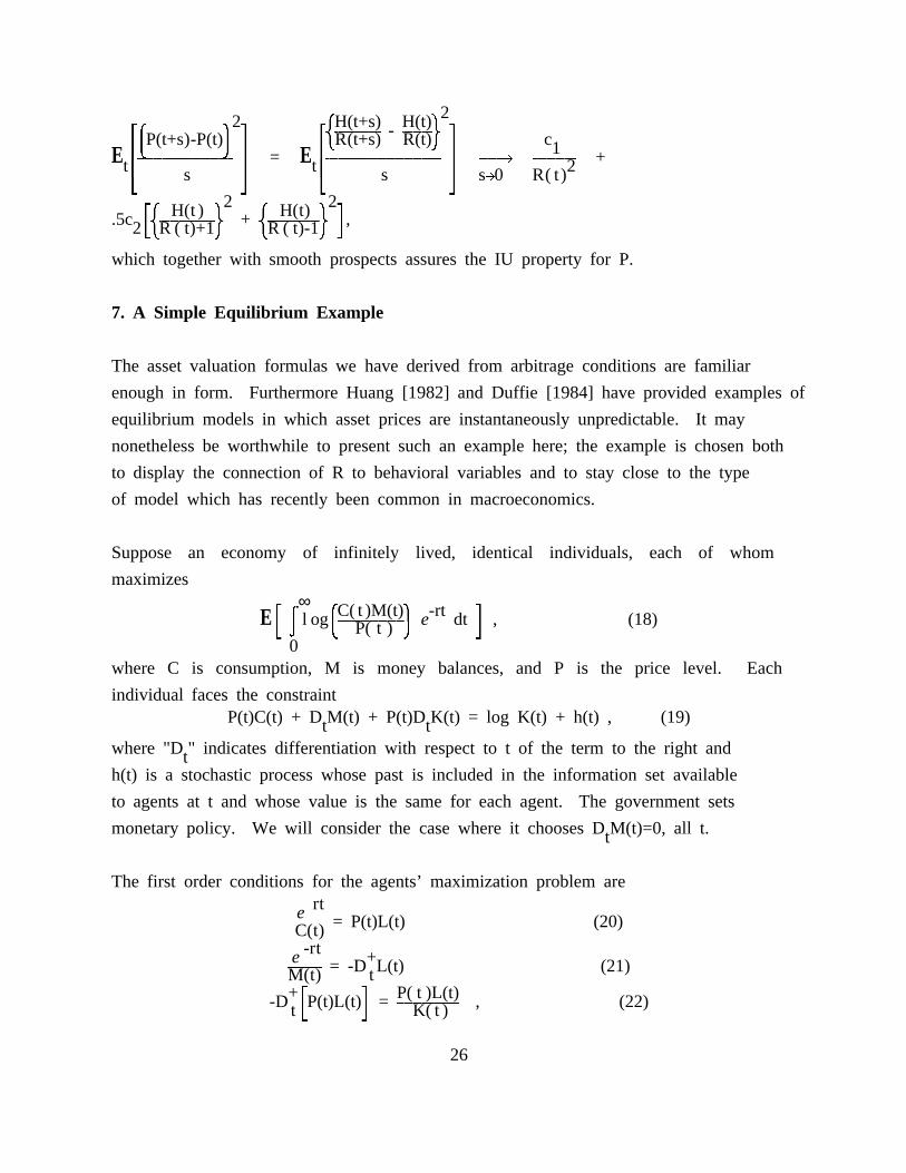
( )22 H(t+s) H(t)#& * $ #--------------------------- - ----------------- $P(t+s)-P(t) R(t+s) R(t) c27 8 2 29 0 2 1E ------------------------------------------------------ = E ----------------------------------------------------------------- --------------L ------------------------- +t2 2 t2 2 2s s sL0 R( t)3 4 3 4

( )2 ( )2# H(t ) H(t) $.5c -------------------------------- + ----------------------------- ,23 R ( t)+1 R ( t)-1 49 0 9 0

which together with smooth prospects assures the IU property for P.

7. A Simple Equilibrium Example

The asset valuation formulas we have derived from arbitrage conditions are familiar

enough in form. Furthermore Huang [1982] and Duffie [1984] have provided examples of

equilibrium models in which asset prices are instantaneously unpredictable. It may

nonetheless be worthwhile to present such an example here; the example is chosen both

to display the connection of R to behavioral variables and to stay close to the type

of model which has recently been common in macroeconomics.

Suppose an economy of infinitely lived, identical individuals, each of whom

maximizes∞

# i &C( t )M(t)* -rt $E l og -------------------------------------- e dt , (18)3 j 7 P( t ) 8 4

0where C is consumption, M is money balances, and P is the price level. Each

individual faces the constraintP(t)C(t) + D M(t) + P(t)D K(t) = log K(t) + h(t) , (19)t t

where "D " indicates differentiation with respect to t of the term to the right andth(t) is a stochastic process whose past is included in the information set available

to agents at t and whose value is the same for each agent. The government sets

monetary policy. We will consider the case where it chooses D M(t)=0, all t.t

The first order conditions for the agents’ maximization problem are----rte

----------------- = P(t)L(t) (20)C(t)-rte +

------------------- = -D L(t) (21)M(t) t+# $ P( t )L(t)-D P(t)L(t) = ----------------------------------- , (22)t3 4 K( t )

26

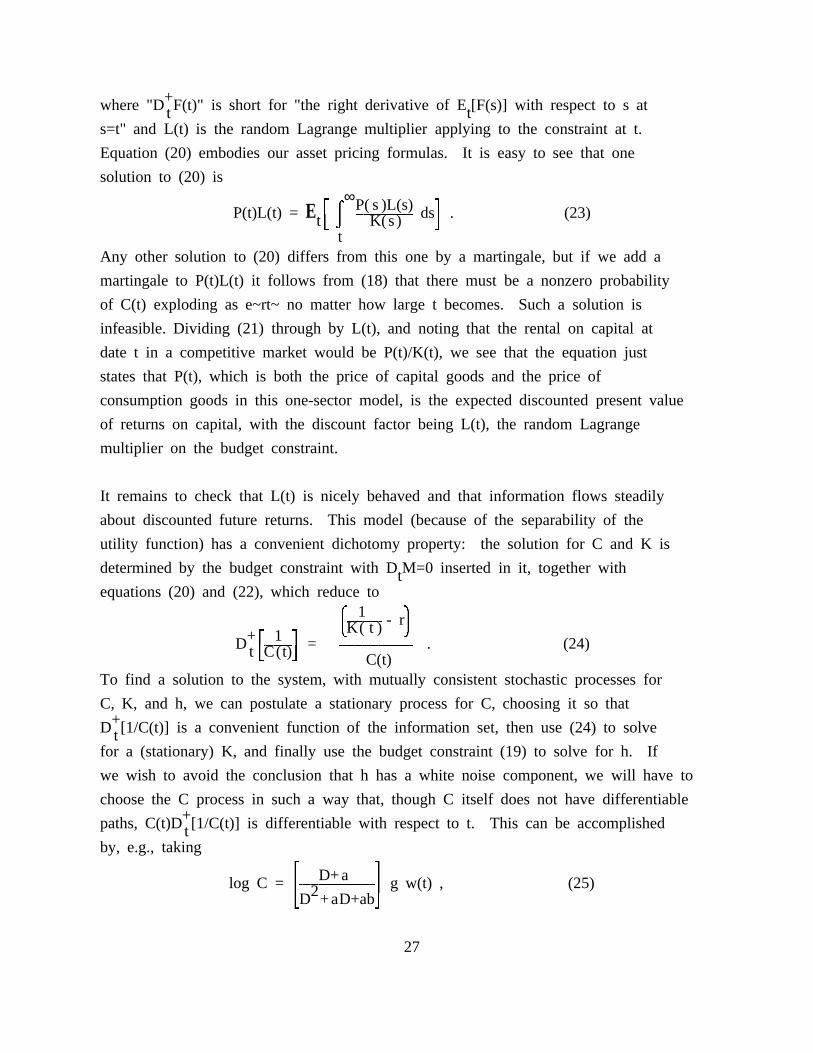
+where "D F(t)" is short for "the right derivative of E [F(s)] with respect to s att ts=t" and L(t) is the random Lagrange multiplier applying to the constraint at t.

Equation (20) embodies our asset pricing formulas. It is easy to see that one

solution to (20) is∞

# i P( s )L(s) $P(t)L(t) = E ------------------------------------- ds . (23)t3 j K(s) 4t

Any other solution to (20) differs from this one by a martingale, but if we add a

martingale to P(t)L(t) it follows from (18) that there must be a nonzero probability

of C(t) exploding as e~rt~ no matter how large t becomes. Such a solution is

infeasible. Dividing (21) through by L(t), and noting that the rental on capital at

date t in a competitive market would be P(t)/K(t), we see that the equation just

states that P(t), which is both the price of capital goods and the price of

consumption goods in this one-sector model, is the expected discounted present value

of returns on capital, with the discount factor being L(t), the random Lagrange

multiplier on the budget constraint.

It remains to check that L(t) is nicely behaved and that information flows steadily

about discounted future returns. This model (because of the separability of the

utility function) has a convenient dichotomy property: the solution for C and K is

determined by the budget constraint with D M=0 inserted in it, together withtequations (20) and (22), which reduce to

& 1 *----------------------- - r7K( t ) 8+# 1 $D ------------------ = ----------------------------------------------- . (24)t3C(t)4 C(t)

To find a solution to the system, with mutually consistent stochastic processes for

C, K, and h, we can postulate a stationary process for C, choosing it so that+D [1/C(t)] is a convenient function of the information set, then use (24) to solvet

for a (stationary) K, and finally use the budget constraint (19) to solve for h. If

we wish to avoid the conclusion that h has a white noise component, we will have to

choose the C process in such a way that, though C itself does not have differentiable+paths, C(t)D [1/C(t)] is differentiable with respect to t. This can be accomplishedt

by, e.g., taking# $D+alog C = 2------------------------------------------------2 g w(t) , (25)23D +aD+ab4

27

where w is a continuous time white noise, the D in (25) is the time-differentiation

operator, and the rational function of D in brackets is interpreted as a one-sided

convolution operator.

It follows from (23) and (20) that C(t) does not have differentiable paths, unless

information is not flowing at t about the integral on the right-hand side of (23).

Thus we could not in (25) have chosen the denominator polynomial in D to have degree

higher by 2 than the numerator without engendering one of the explosive solutions to

(23) we ruled out.

But (25) implies that C has the form# $-ab 2dC(t) = C(t)2---------------------------------------------- w(t)+.5g 2 dt + gC(t)dW(t) , (26)23D +aD+ab 4

assuming w is the derivative of W, a standard Wiener process.

Now (21) above determines the Lagrange multiplier, i.e. the discount factor,

exactly as- r teL(t) = -------------------- . (27)rW

This follows because any other solution to (21) implies a positive probability of

negative L. But then (20) implies

MrP(t) = ------------------- , (28)C(t)

i.e. that the price level is inversely proportional to C. Returning to (26), we see

that a price level inversely proportional to C will certainly have both smooth

prospects and a nonzero Wiener component, hence be IU. We could have obtained the

same conclusion by looking at (23), noting that L is deterministic, and concluding

that unless information is not flowing about the expected future returns to capital,

P will have to be IU.

We could also generate a solution where all the uncertainty concerns jumps. To do

this we would replace (25) by, say, the assumption that C jumps at Poisson-

distributed times with fixed probability per unit time of a jump. To keep C positive

and to ensure that investment and hence output is always well-defined, we have to be

cautious in the choice of the jump distribution. One choice which works is to make

28

a-Z(t) a -Z(t)the jumps go to either C(t)e or C(t)(1-e )e with equal probabilities, and-1with Z(t)=(D+n) logC(t). (a and n are both positive real constants.) This makes the

expected rate of change of C respond negatively to the current level of C, to

preserve stability, but at the same time keeps the expected rate of change from

jumping when C jumps. This is critical because otherwise (24) implies that K jumps

when C jumps, making investment and hence output undefined. But once we have the C

process so defined, we can again solve for K from (24) and P from (28). Again we

will have the conclusion that PC is a constant. Because the jump times are not

foreseen, the implied P process has smooth prospects; and because there is every time

period a chance of a jump, information flows steadily, guaranteeing the IU property

for P.

+Notice that the instantaneous interest rate, -D L(t)/L(t), will have a lowertunconditional expected value for the version of the model with fixed prices than for

the version with fixed M. Also note that the correction for inflation required to

obtain the real rate of return on capital form the nominal rate on bonds is+ +sensitive. The proper correction is D P(t)/P(t), and D log P(t) does not work. Int t

fact, outside our special cases of D M(t)=0 or D P(t)=0, there is in general not tcorrection for expected inflation which will convert the nominal rate to the real

+rate of return on capital, because in (20) D [P(t)L(t)]/P(t)L(t) is not the sum oft+ +D [P(t)]/P(t) and D [L(t)]/L(t) unless the martingale components of P and L aret tuncorrelated.

In versions of the model with M fixed, the determinism of L makes nominal interest

rates constant at r, so bonds of any sort introduced into the model will have

constant prices. It is an exercise left to the reader to verify that if monetary

policy allows M to vary to keep P constant, bonds will have nonconstant prices which

are IU.

6. Conclusion

There are situations where the IU property will certainly fail, but these are mostly

intuitively evident: where, say, information relevant to a security’s returns is

announced at a date fixed in advance, or where the security’s price has been pegged

at a constant either by taking it as numeraire or, in a model with neutral money, by

29

the government’s pegging it with monetary policy. But if information flows steadily

about an asset’s returns, and if the price of the asset does not show rapid

fluctuations over short intervals which allow unbounded returns with bounded variance

over finite intervals, then the asset will have an instantaneously unpredictable

price at almost all dates. To undo this conclusion requires either that information

flow be "lumpy", invalidating the steady flow of information assumption, or that the

discount factor R(t) show discontinuities or nondifferentiability whose form is known

in advance. Except for the easily identified exceptional cases, neither the real

world nor an analytically manageable economic models is likely to generate security

prices which fail to be instantaneously unpredictable.

The notion that asset price changes should be unpredictable in a smoothly

functioning competitive market is justified -- as an approximation, when the time

unit is taken small enough. Tests of the "perfect market hypothesis" do therefore

tell us something about how well a market is functioning. The null hypothesis of

unpredictability will never be exactly true, however, so our attention should focus

on the explanatory power of the regression, rather than on the classical statistical

tests of the null hypothesis.

Furthermore, economic theory shows that the accuracy of the perfect market hypothesis

is only a short run phenomenon. It will be a statistical null hypothesis hard to

reject, even though asset prices changes may be thoroughly predictable at long time

horizons. The frequent success of the hypothesis in statistical tests does not

justify imposing it as an exact theory on forecasting or policy models.

30