Embed Size (px)
Citation preview
Martingale Limit Theoryand
Stochastic Regression Theory
Ching-Zong Wei

Contents
1 Martingale Limit Theory 21.1 Conditional Expectation . . . . . . . . . . . . . . . . . . . . . . . . . 51.2 Martingale . . . . . . . . . . . . . . . . . . . . . . . . . . . . . . . . . 131.3 Basic Inequalities (maximum inequalities) . . . . . . . . . . . . . . . 251.4 Square function inequality . . . . . . . . . . . . . . . . . . . . . . . . 291.5 Series Convergence . . . . . . . . . . . . . . . . . . . . . . . . . . . . 34
2 Stochastic Regression Theory 1092.1 Introduction: . . . . . . . . . . . . . . . . . . . . . . . . . . . . . . . 109
1

Chapter 1
Martingale Limit Theory
Some examples of Martingale:
Example 1.1 Let yi = ayi−1 + εi, where εi i.i.d. with E(εi) = 0, Var(εi) = σ2, andif we estimate a by least squares estimation
a =
∑ni=1 yi−1yi∑ni=1 y
2i−1
a− a =
∑ni=1 yi−1εi∑ni=1 y
2i−1
,
then Sn =∑n
i=1 yi−1εi is a martingale.
Example 1.2 Likelihood Ratio:Given Θ, and
Ln(θ) = fθ(X1, . . . , Xn)
= fθ(Xn|X1, . . . , Xn−1) · fθ(X1, . . . , Xn−1)
=n∏i=2
fθ(Xi|X1, . . . , Xi−1) · fθ(X1),
then Rn(θ) = Ln(θ)Ln(θ0)
, Rn(θ) is a martingale.
2

For example, if Xi = θui + εi, where ui is constant, εi is i.i.d. N(0.1), then
fθ(x1, . . . , xn) = (1√2π
)ne−∑ni=1(xi−θui)
2
2
fθ(x1, . . . , xn)
fθ0(x1, . . . , xn)= e−
∑ni=1(xi−θui)
2
2+
∑ni=1(xi−θ0ui)
2
2
= e(θ−θ0)∑ni=1 uixi−
(θ2−θ20)
2
∑ni=1 u
2i .
Example 1.3 Likelihood: L0 = 1, d logLn(θ)dθ
is a martingale.
logLn(θ) = log fθ(Xn|X1, . . . , Xn−1) + logLn−1(θ)
ui(θ) =d log fθ(Xn|X1, . . . , Xn−1)
dθ=d[logLn(θ)− logLn−1(θ)]
dθ
In(θ) =n∑i=1
Eθ(u2i (θ)|X1, . . . , Xn−1).
Let
Vi(θ) =dui(θ)
dθ=d2 log fθ(Xn|X1, . . . , Xn−1)
dθ2,
sinceEθ(u
2i (θ)|X1, . . . , Xi−1) = −Eθ(Vi(θ)|X1, . . . , Xi−1)
and
Jn(θ) =n∑i=1
Vi(θ),
Then Jn(θ) + In(θ) is a martingale.
Example 1.4 Branching Process with Immigration :Let Zn+1 =
∑Zni=1 Yn+1,i+In+1, where Yj,i is i.i.d. with mean E(Yj,i) = m, Var(Yj,i) =
3

σ2, and In is i.i.d. with mean E(In) = b, Var(In) = λ, then
E(Zn+1|Fn) = mZn + b
Zn+1 = E(Zn+1|Fn) + δn+1
δn+1 = Zn+1 − E(Zn+1|Fn)E(δ2
n+1|Fn) = σ2Zn + λ
Zn+1 = mZn + b+ Zn∑i=1
(Yn+1,i −m) + (In+1 − b)
= mZn + b+√σ2Zn + λ εn+1,
where
εn+1 =δn+1√σ2Zn + λ
.
4

Consider (Ω,F ,P), where
Ω: Sample space
F : σ–algebra ⊂ 2Ω
P: probability
X = ai = Ei, i = 1, . . . , nFX = minimum σ–algebra ⊃ E1, . . . , EnFX1,X2 = σ–algebra ⊃ X1 = ai, X2 = bj i = · · · , j = · · ·Note that FX1,X2 ⊃ FX1 .
Xn is said to be Fn–adaptive if Xn is Fn–measurable (i.e. FXn ⊂ Fn.)
1.1 Conditional Expectation
Main purpose: Given X1 = a1, . . . , Xn = an to find the expectation of Y , i.e. to findE(Y |X1 = a1, . . . , Xn = an).
(Ω,F ,P) is a probability space.Given an event B with P (B) > 0, the conditional probability given B is defined
to be
P (A|B) =P (A ∩B)
P (B)∀A ∈ F ,
then (Ω,F ,P(·|B)) is a probability space.Given X, we can define
E(X|B) =
∫XdP (·|B).
Example 1.5 Let X =∑n
i=1 aiIAi where Ai = X = ai, then E(X|B) =∑n
i=1 aiP (Ai|B).
Ω = ∪∞i=1Bi, where Bi ∩Bj = ∅ if i 6= j.F = σ(Bi), 1 ≤ i <∞E(X|F) =
∑∞i=1E(X|Bi)IBi
Observe that if X =∑n
i=1 aiIAi ,Ω = ∪li=1Bi, Bi ∩Bj = ∅ if i 6= j, then
(i) E(X|F) is F–measurable and E(X|F) ∈ L1,
(ii) ∀ G ∈ F ,∫GE(X|F)dP =
∫GXdP .
5
Sol :
(i) E(X|F) =∑l
i=1E(X|Bi)IBi ,
|E(X|F)| ≤∑l
i=1 |E(X|Bi)| <∞ ⇒ E(X|F) ∈ L1
(ii) ∀ G ∈ F ∫G
E(X|F)dP =
∫G
l∑i=1
E(X|Bi)IBidP
=l∑
i=1
E(X|Bi)P (Bi ∩G)
=l∑
i=1
n∑j=1
ajP (Aj|Bi)P (Bi ∩G)
=n∑j=1
aj(l∑
i=1
P (Aj|Bi)P (Bi ∩G))
=n∑j=1
ajP (Aj ∩G).
Since by hypothesis G ∈ F ,∃ an index set I s.t. G = ∪i∈IBi
l∑i=1
P (Aj|Bi)P (Bi ∩G) =∑i∈I
P (Aj|Bi)P (Bi) =∑i∈I
P (Aj ∩Bi)
= P (Aj ∩ (∪i∈IBi)) = P (Aj ∩G).
Definition 1.1 (Ω,G,P) is a probability space. Let F ⊂ G, X ∈ L1. Define theconditional expectation of X given F to be a random variable that satisfies (i) and(ii).
Existence and Uniqueness:
Uniqueness: Assume Z,W both satisfies (i) and (ii).
Let G = Z > W .
By
6

(i) G is F–measurable,
(ii)∫G(Z −W )dP =
∫GXdP −
∫GXdP = 0
⇒ P (G) = 0.
Recall that Z ≥ 0 a.s. and E(Z) = 0 ⇒ P (Z > 0) = 0.Similarly, P (W > Z) = 0.
Existence: X ≥ 0, X =∑l
i=1 aiIAiDefine ν(G) =
∫GXdP =
∑li=1 aiP (Ai ∩G) ∀ G ∈ F .
Then ν is a (σ–finite) measure on F .
ν P|F = P (P (G) = 0 ⇒ ν(G) = 0)
By Radon-Nikodym theorem ∃ F–measurable function f
s.t.
∫G
fdP =
∫G
fdP = ν(G)
so f = E(X|F) a.s.
• derivative : 4f/4t
• density : contents/unit vol
• ratio
Radon-Nikodym Theorem : Assume that ν and µ are σ–finite measure on F s.t.ν µ. Then ∃ F–measurable function f s.t.∫
A
fdµ = ν(A) ∀A ∈ F (f =dν
dµ).
1. transformation of X −→ new measure
2. FA 6= FB ⇒ E(X|FA) 6= E(X|FB)
Example 1.6
7

1. Discrete : F = σ(Bi, 1 ≤ i <∞) X ∈ L1
E(X|F) =∞∑i=1
∫BiXdP
P (Bi)IBi
2. Continuous : Let f(x, y1, . . . , yn) be the joint density of (X, Y1, . . . , Yn) andg(y1, . . . , yn) =
∫f(x, y1, . . . , yn)dx,
Set f(x|y1, . . . , yn) = f(x,y1,...,yn)
g(Y )I[g(Y ) 6=0], Y = (y1, . . . , yn).
Then E(ϕ(X)|Y1, . . . , Yn) = h(Y1, . . . , Yn) a.s.,
where h(y1, . . . , yn) =∫ϕ(x)f(x|y1, . . . , yn)dx.
We only have to show for any Borel set B ⊂ Rn,
E(h(Y )IB) =
∫B
h(Y )g(Y )dY , Y = (Y1, . . . , Yn)
=
∫B
[
∫ϕ(x)f(x|Y )dx]g(Y )dY
=
∫B
∫ϕ(x)f(x, Y )dxdY
=
∫ ∫ϕ(x)IBf(x, Y )dxdY
= E(ϕ(X)IB)
= E(E(ϕ(X)IB|Y ))
⇒ ϕ(X) = h(Y )
Proposition 1.1 Let X, Y ∈ L1,
1. E[E(X|F)] = E X.Proof :
∫ΩE(X|F)dP =
∫ΩXdP .
2. E(X|∅,Ω) = E X.
3. If X is F–measurable then E(X|F) = X a.s..Proof : Since ∀G ∈ F
∫GE(X|F)dP =
∫GXdP .
4. If X = c ,a constant, a.s. then E(X|F) = c a.s..Proof :
∫GXdP =
∫GcdP, Y ≡ c is F–measurable.
8

5. ∀ constants a, b E(aX + bY |F) = aE(X|F) + bE(Y |F).Proof :
∫G(rhd) =
∫G(lhs).
6. X ≤ Y a.s. ⇒ E(X|F) ≤ E(Y |F).Proof : Use (5), we only show that
X − Y = Z ≥ 0 a.s. ⇒ E(Z|F) ≥ 0 a.s..
Let A = E(Z|F) < 0, then
0 ≤∫A
ZdP =
∫A
E(Z|F)dP ⇒ P (A) = 0.
7. |E(X|F)| ≤ E(|X||F) a.s..
8. |Xn| ≤ Y a.s., Y ∈ L1. If limn→∞Xn = X a.s., then
limn→∞
E(Xn|F) = E(X|F) a.s..
Proof :Set Zn = supk≥n |Xk−X|, then Zn ≤ 2Y . So Zn ∈ L1, and Zn ↓ ⇒ E(Zn|F) ↓ .So ∃Z s.t. limn→∞E(Zn|F) = Z a.s.. We only have to show that Z = 0 a.s..Since |E(Xn|F)− E(X|F)| ≤ E(|Xn −X||F) ≤ E(Zn|F).Note that Z ≥ 0 a.s.. We only have to prove E Z = 0.Since E(Zn|F) ↓ Z, hence
E Z ≤ limn→∞
E(E(Zn|F)) = limn→∞
E(Zn) = E( limn→∞
Zn) = 0
⇒ E Z = 0.
Theorem 1.1 If X is F–measurable and Y,XY ∈ L1, then E(XY |F) = XE(Y |F).Proof :
1. X = IG where G ∈ F∀ B ∈ F ∫
B
E(XY |F)dP =
∫B
XY dP =
∫B
IGY dP =
∫B∩G
Y dP
=
∫B∩G
E(Y |F)dP (Since B ∩G ∈ F)
=
∫B
IGE(Y |F)dP =
∫B
XE(Y |F)dP.
So E(XY |F) = XE(Y |F).
9

2. Find Xn s.t. Xn =∑n2
k=0knI[ kn≤x< k+1
n] − k
nI[− k+1
n<x≤− k
n],
then |Xn| ≤ |X|, and Xn → X a.s..From (1), we obtain that E(XnY |F) = XnE(Y |F).Now XnY → XY a.s.|XnY | = |Xn||Y | ≤ |XY |limn→∞E(XnY |F)
byD.C.T.= E(limn→∞XnY |F) = E(XY |F).
But limn→∞XnE(Y |F) = XE(Y |F) a.s..So E(XY |F) = XE(Y |F).
Theorem 1.2 (Towering)If X ∈ L1 and F1 ⊂ F2, then E[E(X|F2)|F1] = E(X|F1).
Proof : ∀ B ∈ F1 then B ∈ F2 and∫B
E[E(X|F2)|F1]dP =
∫B
E(X|F2)dP (Since B ∈ F1)
=
∫B
XdP (Since B ∈ F2).
So E[E(X|F2)|F1] = E(X|F1) a.s..
Remark 1.1 E[E(X|F1)|F2] = E(X|F1)E[1|F2] = E(X|F1), since E(X|F1) is F2–measurable.
Jensen’s Inequality : If ϕ is a convex function on R and X,ϕ(X) ∈ L1 thenϕ(E(X|F)) ≤ E(ϕ(X)|F) a.s..Proof :
1. Let X =∑k
i=1 aiIAi , where ∪ki=1Ai = Ω, and Ai ∩ Aj = ∅ if i 6= j, then
E(X|F) =k∑i=1
aiE(IAi|F).
Sincek∑i=1
E(IAi|F) = E(k∑i=1
IAi|F) = E(1|F) = 1 a.s.,
10

so
ϕ(E(X|F)) ≤k∑i=1
E(IAi|F)ϕ(ai)
= E(k∑i=1
ϕ(ai)IAi|F) = E(ϕ(X)|F)
2. FindXn as before (i.e., Xn is of the form∑aiIAi , |Xn| ≤ |X|, andXn → Xa.s..)
Then ϕ(E(Xn|F)) ≤ E(ϕ(Xn)|F).First observe that E(Xn|F) → E(X|F)a.s.. By continuity of ϕ,
limn→∞
ϕ(E(Xn|F)) = ϕ( limn→∞
E(Xn|F)) = ϕ(E(X|F))
Fix m,we can find a convex function ϕm such that ϕm(x) = ϕ(x), ∀|x| ≤ m,and |ϕm(x)| ≤ Cm(|x|+ 1), ∀x, and ϕ(x) ≥ ϕm(x), ∀x.Fix m, ∀n,
|ϕm(xn)| ≤ Cm(|xn|+ 1) ≤ Cm(|x|+ 1),
solimn→∞
E[ϕm(xn)|F ] = E[ limn→∞
ϕm(xn)|F ] = E[ϕm(x)|F ],
E[ϕ(x)|F ] ≥ supmE[ϕm(x)|F ] = sup
mlimn→∞
E[ϕm(xn)|F ]
≥ supm
limn→∞
ϕm(E(Xn|F)) = supmϕm[ lim
n→∞E(Xn|F)]
= supmϕm[E(X|F)] = ϕ[E(X|F)] a.s.
Some properties of convex function ϕ :
• If λi ≥ 0,∑n
i=1 λi = 1 then ϕ(∑n
i=1 λixi) ≤∑n
i=1 λiϕ(xi)
• The geometry property
• ϕ is continuous(since right-derivative and left-derivative exist)
11

Corollary 1.1 If X ∈ Lp, p ≥ 1 then E(X|F) ∈ Lp.Proof : Since ϕ(x) = |x|p is convex if p ≥ 1, then
|E(X|F)|p ≤ E(|X|p|F) a.s.
andE|E(X|F)|p ≤ EE(|X|p|F) = E|X|p <∞.
Homework :
1. If p > 1 and 1p
+ 1q
= 1,X ∈ Lp, Y ∈ Lq, then
E(|XY ||F) ≤ E(|X|p|F)1pE(|Y |q|F)
1q a.s..
2. If X ∈ L2 and Y ∈ L2(F) = U : U ∈ L2 and U is F–measurable, then
E(X − Y )2 = E(X − E(X|F))2 + E(E(X|F)− Y )2.
Thereforeinf
Y ∈L2(F)E(X − Y )2 = E(X − E(X|F))2.
Proof :
E(X − Y )2 = E(X − E(X|F) + E(X|F)− Y )2
= E(X − E(X|F))2 + E(E(X|F)− Y )2
+2E[(X − E(X|F))(E(X|F)− Y )].
Lemma 1.1 E(X − E(X|F))U = 0 if U ∈ L2(F).proof:
E[E((X − E(X|F))U |F)] = EU [E((X − E(X|F))|F ]= EU [E(X|F)− E(X|F)] = EU · 0 = 0.
Application : Bayes Estimate (X1, · · · , Xn) ∼ f(~x|θ) , θ ∈ L2, Xi ∈ L2. UseX1, · · · , Xn to estimate θ.Method : find θ(X1, · · · , Xn) ∈ L2 such that E(θ − θ)2 is minimum.
12

Remark 1.2 Let Fn = σ(X1, · · · , Xn). Then θ is Fn–measurable⇔ ∃ measurable function h such that θ = h(X1, · · · , Xn) a.s.So θn = E(θ|Fn) is the solution.
Question : In what sense θn −→ θ ?
1.2 Martingale
(Ω,F ,P)Fn ⊂ F ,Fn ⊂ Fn+1 : history(filtration)
Definition 1.2
(i) Xn is Fn–adaptive ( or adapted to Fn ) if Xn is Fn–measurable ∀n.
(ii) Yn is Fn–predictive ( predictive w.r.t. Fn ) if Yn is Fn−1–measurable ∀n.
(iii) The σ–fields Fn = σ(X1, · · · , Xn) is said to be the natural history of Xn.( Itis obvious Fn ↑. )
(iv) Xn, n ≥ 1 is said to be a martingale w.r.t. Fn, n ≥ 1 ,if
(1) Xn is Fn–adaptive.(2) E(Xn|Fn−1) = Xn−1, ∀n ≥ 2.
(3) εn, n ≥ 1 is said to be a martingale difference sequence w.r.t. Fn, n ≥ 0if E(εn|Fn−1) = 0 a.s., ∀n ≥ 1.
Remark 1.3 If Xn, n ≥ 1 is a martingale w.r.t. Fn, n ≥ 1 and E(X1) = 0,then ε1 = X1, εn = Xn − Xn−1 for n ≥ 2 is a martingale difference sequence w.r.t.Fn, n ≥ 0, where F0 = ∅,Ω, E(ε1|F0) = E(X1|F0) = E(X1) = 0.
If εn, n ≥ 1 is a martingale difference w.r.t. Fn, n ≥ 0,Yn, n ≥ 1 is Fn, n ≥0–predictive, and εn ∈ L1, Ynεn ∈ L1, then Sn =
∑ni=1 Yiεi is a martingale w.r.t.
13

Fn, n ≥ 0.Proof :
E(Sn|Fn−1) = E(Ynεn + Sn−1|Fn−1)
= E(Ynεn|Fn−1) + Sn−1 = YnE(εn|Fn−1) + Sn−1
= Yn · 0 + Sn−1 = Sn−1 a.s..
Example 1.7
(a) If εi are independent r.v.′s with E(εi) = 0, and V ar(εi) = 1, ∀i. Let Sn =∑ni=1 εi, and Fn = σ(ε1, · · · , εn), then E(εn|Fn−1) = E(εn) = 0.
(b) Let Xn = ρXn−1 +εn, |ρ| < 1, where εn are i.i.d. with E(εn) = 0, E(ε2n) <∞ and
X0 ∈ L2 is independent of εi, i ≥ 1, then∑n
i=1Xi−1εi is a martingale w.r.t.Fn, n ≥ 0, where Fn = σ(X0, ε1, · · · , εn), ∀n ≥ 0.proof :
Xn = ρ2Xn−2 + ρεn−1 + εn
= · · · = ρnX0 + ρn−1ε1 + · · ·+ εn.
(c) Bayes estimate : θn = E(θ|Fn) where Fn ↑,
E(θn+1|Fn) = E(E(θ|Fn+1)|Fn) = E(θ|Fn) = θn.
(d) Likelihood Ratio : Pθ, dPθ = fθ(X1, · · · , Xn)dµ
Yn(θ, θ0, X1, · · · , Xn) =fθ(X1, · · · , Xn)
fθ0(X1, · · · , Xn)=
dPθ/dµ
dPθ0/dµ=
dPθdPθ0
Fn = σ(X1, · · · , Xn)
Ln(θ,X1, · · · , Xn) = fθ(Xn|X1, · · · , Xn−1)Ln−1(θ,X1, · · · , Xn−1).
14

Fix θ0, θ, thenYn(θ),Fn, n ≥ 1 is a martingale
Eθ0(Yn(θ)|Fn−1) = Eθ0(Ln(θ)
Ln(θ0)|Fn−1)
= Eθ0(fθ(Xn|X1, · · · , Xn−1)
fθ0(Xn|X1, · · · , Xn−1)· Ln−1(θ)
Ln−1(θ0)|Fn−1)
=Ln−1(θ)
Ln−1(θ0)Eθ0(
fθ(Xn|X1, · · · , Xn−1)
fθ0(Xn|X1, · · · , Xn−1)|Fn−1)
= Yn−1(θ)
∫fθ(xn|X1, · · · , Xn−1)
fθ0(xn|X1, · · · , Xn−1)· fθ0(xn|X1, · · · , Xn−1)dxn.
i.e., E(ϕ(X)|X1, · · · , Xn) =
∫ϕ(x)f(x|X1, · · · , Xn)dx.
(e) d logLn(θ)dθ
,Fn = σ(X1, · · · , Xn) is a martingale if∫∂fθ(xn|X1, · · · , Xn−1)
∂θdxn =
∂
∂θ
∫fθ(xn|X1, · · · , Xn−1)dxn = 0.
Eθ(d logLn(θ)
dθ|Fn−1)
= Eθ(d log fθ(Xn|X1, · · · , Xn−1)
dθ+d logLn−1(θ)
dθ|Fn−1)
= Eθ[∂fθ(Xn|X1,··· ,Xn−1)
∂θ
fθ(Xn|X1, · · · , Xn−1)|Fn−1] +
d logLn−1(θ)
dθ
=
∫ ∂fθ(xn|X1,··· ,Xn−1)∂θ
fθ(xn|X1, · · · , Xn−1)· fθ(xn|X1, · · · , Xn−1)dxn +
d logLn−1(θ)
dθ
=d logLn−1(θ)
dθ.
Lemma : If Xn is Fn–adaptive and Xn ∈ L1, then S1 = X1, Sn = X1 +∑ni=2(Xi − E(Xi|Fi−1)) is a martingale w.r.t. Fn, n ≥ 1.
proof : n ≥ 2,
∵ E(Sn|Fn−1) = X1 +n∑i=2
Xi − E(Xi|Fi−1) + E[(Xn − E(Xn|Fn−1))|Fn−1],
∴ E[(Xn − E(Xn|Fn−1))|Fn−1] = E(Xn|Fn−1)− E(Xn|Fn−1) = 0.
15

(f) Let
un(θ) =d log fθ(Xn|X1, . . . , Xn−1)
dθ,
d logLn(θ)
dθ=
n∑i=1
ui(θ),
I(θ) =n∑i=1
E[u2i (θ)|Fi−1],
dun(θ)
dθ= vn(θ),
J(θ) =n∑i=1
vn(θ),
then J(θ)+I(θ) is a martingale, and J(θ)−∑m
i=1E(vi(θ)|Fi−1) is a martingale.We only have to show that
E[vi(θ)|Fi−1] = −E[u2i (θ)|Fi−1] a.s..
Example : Xn = θXn−1 + εn, n = 1, 2, . . ., and X0 ∼ N(0, c2) is independentof i.i.d. sequence εn ∼ N(0, σ2). Assume that σ2 and c2 are known, then
Ln(θ,X0, . . . , Xn) = fθ(X0)fθ(X1|X0) · · · fθ(Xn|X0, . . . , Xn−1)
=1√2πc
e−x202c2 · · · 1√
2πσe−
(xn−θxn−1)2
2σ2
= (1√2π
)n+1 1
c
1
σne−[
x202c2
+ 12σ2
∑ni=1(xi−θxi−1)2].
Hence
logLn(θ) =n+ 1
2log(2π)− log c− n log σ − [
x20
2c2+
1
2σ2
n∑i=1
(xi − θxi−1)2],
therefore
d logLn(θ)
dθ=
1
σ2
n∑i=1
xi−1(xi − θxi−1) =1
σ2
n∑i=1
xi−1εi.
16

i.e., ui(θ) =1
σ2Xi−1(Xi − θXi−1) ⇒ u2
i (θ) =1
σ4X2i−1(Xi − θXi−1)
2.
Then
E[u2i (θ)|Fi−1] =
1
σ4X2i−1E[(Xi − θXi−1)
2|Fi−1]
=1
σ4X2i−1σ
2 =X2i−1
σ2,
so
I(θ) =1
σ2
n∑i=1
X2i−1,
vi(θ) =dui(θ)
dθ= −
X2i−1
σ2,
J(θ) =n∑i=1
vi(θ) = − 1
σ2
n∑i=1
X2i−1.
⇒ I(θ) + J(θ) = 0.
And∑n
i=1 u2i (θ) +
∑ni=1E[vi(θ)|Fi−1] is also a martingale, since
1
σ4
n∑i=1
X2i−1[Xi − θXi−1]
2 − 1
σ2
n∑i=1
X2i−1 =
1
σ4
n∑i=1
X2i−1[ε
2i − σ2],
E[ε2 − σ2|Fi−1] = E(ε2 − σ2) = σ2 − σ2 = 0.
Definition 1.3 An Fn, n ≥ 1– adaptive seq. Xn is defined to be a sub–martingale(super–martingale) if E(Xn|Fn−1) ≥ (≤)Xn−1 for n = 2, . . ..
(1)Intuitive : martingale — constantsubmartingale — increasingsupermartingale — decreasing
(2)Game : martingale — fair gamesubmartingale — favorable gamesuppermartingale — infarovable game
17

Theorem 1.3
(i) Assume that Xn,Fn is a martingale. If ϕ is convex and ϕ(Xn) ∈ L1, thenϕ(Xn)Fn is a submartingale.
(ii) Assume that Xn,Fn is a submartingale. If ϕ is convex, increasing and E[ϕ(Xn)] ∈L1, then ϕ(Xn),Fn is a submartingale.
Proof : By Jensen inequality,
E[ϕ(Xn)|Fn−1] ≥ ϕ(E[Xn|Fn−1]) = ϕ(Xn−1).
For examples, ϕ(x) = |x|p, p ≥ 1 or ϕ(x) = (x− a)+.
Corollary 1.2 If Xn,Fn is a martingale, and Xn ∈ Lp with p ≥ 1, then h(n) =E|Xn|p is an increasing function.Proof : Since |Xn|p,Fn is a submartingale,
EE(|Xn+1|p|Fn) ≥ E|Xn|p.
Prove that Xn =∑n
i=1 εi, where ε′is are i.i.d. r.v.′s with E(εi) = 0, and E|εi|3 <∞,then
E|Xn|3 ≤ E|Xn+1|3 ≤ . . . .
(iii) [Gilat,D.(1977) Ann. Prob. 5,pp.475-481]For a nonnegative submartingale Xn, σ(X1, . . . , Xn), there is a martingale
Yn, σ(Y1, . . . , Yn) s.t. XnD= |Yn|.
(iv) Assume that Xn, σ(X1, . . . , Xn) is a nonnegative submartingale. If ϕ is con-vex and ϕ(Xn) ∈ L1, then there is a submartingale Zn, σ(Z1, . . . , Zn) s.t.ϕ(Xn)
D= Zn.
Proof : Let ψ(X) = ϕ(|X|). Then ψ(X) is a convex function. By Gilat’s
theorem, ∃ martingale Yn s.t. XnD= |Yn|, so
ϕ(Xn)D= ϕ(|Yn|) = ψ(Yn) = Zn,
which is a submartingale by (i).
18

Homework : Assume that Xn,Fn is a submartingale. If ∃ m > 1 s.t. E(Xm) =E(X1), then Xi,Fi, 1 ≤ i ≤ m is a martingale.
Definition 1.4 Let N∞ = 1, 2, . . . ,∞, and T : Ω → N∞. Then T is said to be aFn–stopping time if T = n ∈ Fn, n = 1, 2, . . . .
Remark 1.4 Let F∞ = ∨nFn. Since T = ∞ = T < ∞c and T < ∞ =∪nT = n ∈ F∞ so T = ∞ ∈ F∞.
We said that a stopping time T is finite if PT = ∞ = 0.
Remark 1.5 Since T ≥ n = T < nc ∈ Fn−1, then
T ≤ n ∈ Fn, ∀ n⇔ T = n ∈ Fn, ∀ n.
Definition 1.5 Let T be an Fn–stopping time. The pre–T σ–field FT is defined tobe Λ ∈ F : Λ ∩ T = n ∈ Fn,∀ n ∈ N∞.
If Λ ∈ FT , then Λ = ∪n∈N∞(Λ ∩ T = n) ∈ F∞, so FT ⊂ F∞.
Example 1.8 Let Xn be Fn–adaptive ∀ Borel set Γ, we define T = infn : Xn ∈ Γ.Then T is an Fn–stopping time. (inf Ø = ∞).Proof : T = k = X1 6∈ Γ, . . . , Xk−1 6∈ Γ, Xk ∈ Γ ∈ Fk.
Theorem 1.4 Assume that T1 and T2 are Fn–stopping times.
(i) Then so are T1 ∧ T2 and T1 ∨ T2.
19

(ii) If T1 ≤ T2 then FT1 ⊂ FT2.
Proof :
(i) T1 ∧ T2 ≤ n = T1 ≤ n ∪ T2 ≤ n ∈ FnT1 ∨ T2 ≤ n = T1 ≤ n ∩ T2 ≤ n ∈ Fn
(ii) Let Λ ∈ FT1, then Λ∩ T1 ≤ n ∈ Fn. Since T2 ≤ n ∈ Fn, we have Λ∩ T1 ≤n ∩ T2 ≤ n ∈ Fn and Λ ∩ T1 ≤ n ∩ T2 ≤ n = Λ ∩ T2 ≤ n ∈ FT2, soΛ ∈ FT2 .
Theorem 1.5 (Optional Sampling Theorem)Let α and β be two Fn–stopping times s.t. α ≤ β ≤ K where K is a positive
integers. Then for any (sub or super) martingale Xn,Fn,Xα,Fα;Xβ,Fβ is a(sub or super) martingale.Proof : We only have to consider the case when Xn is a submartingale.Lemma : Assume that β is an Fn–stopping time s.t. β ≤ K. If Xn,Fn is asubmartingale then
E[Xβ|Fn] ≥ Xn a.s. on β ≥ nE[Xβ|Fn]I[β≥n] ≥ XnI[β≥n] a.s.
Proof of Lemma : It is sufficient to show that
∀ A ∈ Fn∫A
XβI[β≥n]dp ≥∫A
XnI[β≥n]dp
Let A = Un > E(Z|Fn), E(Z|Fn) ≥ Un ∈ Fn
⇔ ∀ A ∈ Fn,∫A
Zdp ≥∫A
Udp
⇔ ∀ A ∈ Fn,∫A
(Z − U)dp ≥ 0
⇔∫A
E(Z|Fn)dp ≥∫A
Udp
⇔∫A
[E(Z|Fn)− U ]dp = 0.
20

∫A
XnI[β≥n]dp =
∫A∩[β≥n]
Xndp =
∫A∩[β=n]
Xndp+
∫A∩[β≥n+1]
Xndp
≤∫A∩[β=n]
Xβdp+
∫A∩[β≥n+1]
Xn+1dp.
Since B ∈ Fn, ∫B
E[Xn+1|Fn]dp =
∫B
Xn+1dp ≥∫B
Xndp.
We have that∫A
XnI[β≥n]dp ≤∫A∩[β=n]
Xβdp+ . . .+
∫A∩[β=K]
Xβdp+
∫A∩[β≥K+1]
XK+1dp
=
∫A∩[n≤β≤K]
Xβdp =
∫A∩[n≤β]
Xβdp.
Continuation of the proof of the theorem :It is sufficient to show that ∀ Λ ∈ Fα,
∫ΛXβdp ≥
∫ΛXαdp. Given Λ ∈ Fα, A =
∪kn=1(Λ ∩ α = n). It is sufficient to show ∀ 1 ≤ n ≤ K,∫Λ∩[α=n]
Xβdp ≥∫
Λ∩[α=n]
Xαdp =
∫Λ∩[α=n]
Xndp.
However,∫
Λ∩[α=n]Xβdp =
∫Λ∩[α=n]
E(Xβ|Fn)dp. Since α = n ⊂ β ≥ n (since
β ≥ α = n), we have∫
Λ∩[α=n]E(Xβ|Fn)dp ≥
∫Λ∩[α=n]
Xndp,
∀ n, Xα ≤ x ∪ α = n = Xn ≤ x ∩ α = n ∈ Fn
So Xα ≤ x ∈ Fα.
Remark 1.6 If α = 1,∀ β ≤ K, we have EXβ = EX1, then Xn,Fn is a martin-gale.
How to prove the convergence of a sequence:
1. Find the limit X, try to show |Xn −X| → 0.
21

2. Without knowing the limit:
(i) Cauchy sequence supm>n |Xn −Xm| → 0 as n→∞(ii) limit set ,[lim infXn, lim supXn] = A
(a) lim infXn = lim supXn
(b) ∀ a ∈ A,ψ(a) = 0 and ψ has a unique root.
Consider
lim infXn < lim supXn = ∪ a<brationals
lim infXn < a < b < lim supXn
α1 = infm : Xm ≤ aβ1 = infm > α1 : Xm ≥ b
...
αk = infm > βk−1 : Xm ≤ aβk = infm > αk : Xm ≥ b,
and define upcrossing number Un = Un[a, b] = supj : βj ≤ n, j < ∞. Note that ifα′i = αi ∧ n, β′i = βi ∧ n then α′n = β′n = n.
Then define τ0 = 1, τ1 = α′1, . . . , τ2n−1 = α′n, and τ2n = β′n. Clearly, τn = n.If Xn,Fn is a submartingale, then Xτk ,Fτk , 1 ≤ k ≤ n is a submartingale by
optional sampling theorem. ( Since τk ≤ n ∀ 1 ≤ k ≤ n. )
Theorem 1.6 (Upcrossing Inequality)If Xn,Fn is a submartingale, then (b− a)EUn ≤ E(Xn − a)+ − E(X1 − a)+.
Proof : Observe that the upcrossing number Un[0, b− a] of (Xn − a)+ is the same asUn[a, b] of Xn. Furthermore,(Xn−a)+,Fn is also a martingale. ϕ(x) = (x−a)+ is aconvex function. Hence we only have to show the case Xn ≥ 0 a.s. and Un = Un[0, c].Now consider
Xn −X1 = Xτn −Xτn−1 + . . .+Xτ1 −Xτ0 =n−1∑i=0
(Xτi+1−Xτi) =
∑i:even
+∑i:odd
,
∵∑i:odd
(xτi+1−Xτi) ≥ UnC,
∴ EXn − EX1 ≥ CEUn + E(∑i:even
) ≥ CEUn +∑i:even
(EXτi+1− EXτi) ≥ CEUn.
22

Theorem 1.7 (Global convergence theorem)Assume that Xn,Fn is a submartingale s.t. supnE(X+
n ) < ∞. Then Xn con-verges a.s. to a limit X∞ and E|X∞| <∞.Proof : We only have to show that
P [lim infXn < a < b < lim supXn] = 0. (∗)
Let U∞[a, b] be the upcrossing number of Xn. Then lim infXn < a < b <lim supXn ⊂ ∪∞[a, b] = ∞ and Un[a, b] ↑ U∞[a, b],
EU∞[a, b] = limn→∞
E(Un[a, b])
≤ supn
(E(Xn − a)+ − E(X1 − a)+)/(b− a) <∞,
so U∞[a, b] <∞ a.s., and P [U∞[a, b] = ∞] = 0.This implies (∗). Now
E|Xn| = EX+n + EX−
n = 2EX+n − (EX+
n − EX−n )
= 2EX+n − EXn ≤ 2EX+
n − EX1,
so supnE|Xn| ≤ 2 supnEX+n − EX1 <∞.
By Fatou’s Lemma,
E|X∞| = E( limn→∞
|Xn|) ≤ lim inf E|Xn| ≤ supnE|Xn| <∞.
Remark 1.7 Xn ↑, supnEX+n <∞ : upper bound.
Corollary 1.3 If Xn is a nonnegative supermartingale then ∃ X ∈ L′ s.t. Xna.s.→
X.Proof : Since −Xn is a nonpositive submartingale and E(−Xn)
+ = 0, ∀ n.
Example 1.9
23

1. Likelihood Ratio
Yn(θ) =Ln(θ)
Ln(θ0)≥ 0.
So Yn(θ) → Y (θ) a.s. (Pθ0), (Y (θ) = 0 if θ1, θ0 are distinctable.)
2. Baye’s est.
θn = E[θ|X1, . . . , Xn], E(θ2) <∞E|θn| ≤ EE(|θn||X1, . . . , Xn) = E|θn| <∞.
So supnE|θn| <∞, and θna.s.→ θ∞.
Definition 1.6 Xn is said to be uniformly integrable(u.i.) if ∀ ε > 0,∃ A s.t.
supn
∫|Xn|>A
|Xn|dp ≤ ε or limA→∞
supn
∫|Xn|>A
|Xn|dp→ 0.
Theorem 1.8 Xn is u.i. ⇐⇒
(i) supnE|Xn| <∞, and
(ii) ∀ ε > 0,∃ δ > 0 s.t. ∀ E ∈ F , P (E) < δ ⇒ supn∫E|Xn|dP < ε.
How to prove Xn is u.i. ?
1. If Z = supn |Xn| ∈ L′ then Xn is u.i..Proof :
(i) obvious,since E|Xn| ≤ E(Z) <∞(ii) ∫
E
|Xn|dP ≤∫E
ZdP ≤∫E
ZI[Z≤c]dP +
∫E
ZI[Z>c]dP
≤ cP (E) +
∫Z>c
ZdP
24

2. If ∃ Borel–measurable function f : [0,∞) 7→ [0,∞) s.t. supnEf(|Xn|) <∞ and
limt→∞f(t)t
= ∞, then Xn is u.i..
Theorem 1.9 Assume that Xnp→ X , then the following statements are equivalent.
(i) |Xn|p is u.i.
(ii) XnLp→ X, (i.e.E|Xn −X|p n→∞−→ 0)
(iii) E|Xn|pn→∞−→ E|X|p
Remark 1.8 If XnD→ X and |Xn|p is u.i., then E|Xn|p
n→∞−→ E|X|p.Proof : We can reconstruct the probability space and r.v.’s X ′
n, X′,
s.t. X ′nD= Xn, X
′ D= X and X ′na.s.→ X ′.
Ex. Let XnD→ N(0, σ2) and X2
n is u.i., then E(X2n)
n→∞−→ σ2. How to knowmax1≤i≤n|Xn|p ∈ L1 ?
1.3 Basic Inequalities (maximum inequalities)
Theorem 1.10 (Fundamental Inequality)If Xi,Fi, i ≤ i ≤ n is a submartingale, then ∀ λ
λP [max1≤i≤n
Xi > λ] ≤ E(XnI[max1≤i≤nXi>λ]).
Proof : Define τ = infi : Xi > λ, (recall : inf Ø = ∞), then max1≤i≤nXi > λ =τ ≤ n. On the set τ = k ≤ n, Xτ > λ, then
λP [τ = k] ≤∫
[τ=k]
XτdP =
∫[τ=k]
XkdP ≤∫
[τ=k]
XndP
Sinceτ = k ⇔ X1 ≤ λ, . . . , Xk−1 ≤ λ,Xk > λ,
then
λP [max1≤i≤n
Xi > λ] = λ
n∑k=1
P [τ = k] ≤∫
[τ≤n]
XndP =
∫[max1≤i≤nXi>λ]
XndP.
25

Theorem 1.11 (Doob’s Inequality)If Xi,Fi, 1 ≤ i ≤ n is a martingale, then ∀ p > 1
‖Xn‖p ≤ ‖ max1≤i≤n
|Xi|‖p ≤ q‖Xn‖p ,
where ‖X‖p = (E|X|p)1p and 1
p+ 1
q= 1.
Proof : Since |Xn|,Fn is a submartingale, by the theorem. Let Z = max1≤i≤n |Xi|,then
E(Zp) = p
∫ ∞
0
xp−1P [Z > x]dx
≤ p
∫ ∞
0
xp−2E(|Xn|I[Z>x])dx = pE[|Xn|∫ ∞
0
I[Z > x]xp−2dx]
≤ pE[|Xn|∫ Z
0
xp−2dx] = pE[|Xn|Zp−1
p− 1]
≤ p
p− 1‖Xn‖p‖Zp−1‖q =
p
p− 1‖Xn‖p[E(Zp)]
1q .
Hence
‖Zp−1‖q = E(Zp−1)q1/q = [E(Zp)]1/q,
‖Z‖p = [E(Zp)]1/p = [E(Zp)]1−1q ≤ q‖Xn‖p.
Note that‖ max
1≤i≤n|Xi|‖p = ∞ ⇒ q‖Xn‖p = ∞.
Corollary 1.4 If Xn,Fn, n ≥ 1 is a martingale s.t. supnE|Xn|p < ∞ for somep > 1 then |Xn|p is u.i. and Xn converges in Lp.Proof : p > 1 ⇒ supnE|Xn| < ∞ so Xn converges a.s. to a r.v. X. By Doob’sinequality:
‖ max1≤i≤n
|Xi|‖p ≤ q‖Xn‖p ≤ q supn‖Xn‖p <∞
By the Monotone convergence theorem:
E sup1≤i≤∞
|Xi|p = limn→∞
E sup1≤i≤n
|Xi|p ≤ q supnE|Xn|p <∞
So sup1≤i≤∞ |Xi|p ∈ L1, |Xn|p is u.i. and XnLp−→ X.
26
Homework : Show without using martingale convergence theorem that if Xn,Fnis a martingale and supnE|Xn|p <∞ for some p > 1 then Xn converges a.s.
Ex.( Bayes Est. ) θn = E[θ|X1, . . . , Xn]. If θ ∈ L2 then θna.s.→ θ∞ and E[θn−θ∞]2 → 0.
pf: Eθ2n ≤ Eθ2 <∞(p = 2).
What is θ∞ ? Is θ∞ equal to E[θ|Xi, i ≥ 1]?
Theorem 1.12 If X ∈ L1, Xn = E(X|Fn) and X∞ = limn→∞Xn then (i) Xn isu.i., and (ii) X∞ = E(X|F∞) where F∞ = ∨∞n=1Fn.
pf: Fix n, Xn,Fn, X,F is a martingale. Therefore, |Xn|,Fn, |X|,F is a sub-
martingale. So∫|Xn|>λ |Xn|dP ≤
∫|Xn|>λ |X|dP . Now P|Xn| > λ ≤ E|Xn|
λ≤
E|X|λ→ 0. ∫
|Xn|>λ |X|dP ≤ cP|Xn| > λ+∫|X|>c |X|dP
≤ cE|X|λ
+∫|X|>c |X|dP
⇒ supnE|Xn|I[|Xn|>λ] ≤ c
E|X|λ
+
∫|X|>c
|X|dP
limλ→∞
supnE|Xn|I[|Xn|>λ] ≤
∫|X|>c
|X|dP ∀ c
Therefore, XnL1
→ X∞. So ∀ Λ ∈ F ,∫
ΛXndP
n→∞→∫
ΛX∞dP . Since |
∫ΛXndP −∫
ΛX∞dP | ≤
∫Λ|Xn −X∞|dP ≤ E|Xn −X∞| → 0. Fix n,Λ ∈ Fn,∀ m ≥ n∫
Λ
XdP =
∫Λ
XndP =
∫Λ
XmdP =
∫Λ
X∞dP
Let G = Λ :∫
ΛXdP =
∫ΛX∞dP. Then G is a σ–field s.t. G ⊃ ∪∞n=1Fn. So
G ⊃ ∨∞n=1Fn = F∞. Observe that X∞ is F∞–measurable. Hence E(X|F) = X∞.
Corollary 1.5 Assume that θ ∈ L2, θn = E(θ|X1, . . . , Xn) and θ∞ = E(θ|Xi, i ≥ 1).
If ∃ θn = θn(X1, . . . , Xn) s.t. θnp→ θ then θ∞ = θ a.s.
pf: Since θnp→ θ. Let Fn = σ(X1, . . . , Xn). So ∃ nj s.t. θnj
a.s.→ θ as nj → ∞.Hence θ is F∞ = σ(Xi, i ≥ 1) measurable. By the theorem stated above, we getθ∞ = E[θ|F∞] = θ a.s.
27

Example: yi = θxi + εi,Xi : constant,θ ∈ L2 with known density f(θ),εi i.i.d.N(0, σ2), σ2 known, and εi is independent of θ.
θn = E(θ|Y1, . . . , Yn) =µc2
+∑ni=1XiYiσ2
1c2
+∑ni=1X
2i
σ2
Assume that f(θ) ∼ N(µ, c2), µ, c2 known.
g(θ, y1, . . . , yn) =1√2πc
e−(θ−µ)2
2c2 (1√2πσ
)ne−∑ni=1(yi−θxi)
2
2σ2
g(θ|y1, . . . , yn) = g(θ,y1,...,yn)∫g(θ,y1,...,yn)dθ
∝ K(y1, . . . , yn)e−( 1
2c2+
∑ni=1X
2i
2σ2 )θ2+(µ2
c2+
∑ni=1 xiyiσ2 )θ
When∑∞
i=1X2i <∞
θnn→∞−→
µc2
+∑∞i=1X
2i
σ2 θ +∑∞i=1Xiεiσ2
1c2
+∑∞i=1X
2i
σ2
= θ∞
∼ N(µ,
∑∞i=1X
2i
σ2 c2 +(∑∞i=1X
2i )σ2
σ4
( 1c2
+∑∞i=1X
2i
σ2 )2)D6= θ
When∑∞
i=1X2i →∞
θn ∼∑n
i=1 xiyi∑ni=1 x
2i
= θ +
∑ni=1 xiεi∑ni=1 x
2i
a.s.→ θ
In general, let θn =∑ni=1 xiyi∑ni=1 x
2i
. When∑n
i=1 x2i →∞,
E(θn − θ)2 = E∑n
i=1 xiεi∑ni=1X
2i
2 =σ2∑ni=1 x
2i
→ 0
So θnp→ θ. By our theorem, θn → θ a.s. or L2.
How to calculate the upper and lower bound of E|Xn|p and E|∑n
i=1Xiεi|p ?
28

1.4 Square function inequality
Let Xn,Fn be a martingale and d1 = X1,di = Xi −Xi−1 for i ≥ 2.
Theorem 1.13 (Burkholder’s inequality)∀ 1 < p <∞, ∃ C1 and C2 depending only on p such that
C1E|n∑i=1
d2i |p/2 ≤ E|Xn|p ≤ C2E|
n∑i=1
d2i |p/2
Cor. For p > 1, ∃C ′2 depending only on p s.t.
C1E|n∑i=1
d2i |p/2 ≤ E(X∗
n)p ≤ C ′
2E|n∑i=1
d2i |p/2
where X∗n = max1≤i≤n |Xi| and C1 is defined by the theorem.
proof:Since E(X∗
n)p ≥ E|Xn|p =⇒ lower half is obtained.
By Doob’s inequality: ‖X∗n‖p ≤ q‖Xn‖p
So E(X∗n)p = ‖X∗
n‖pp ≤ qpE|Xn|p ≤ qpC2E|∑n
i=1 d2i |p/2
Remark: When di are independent, it is called Marcinkiewz-Zygmund inequality.Note that for p ≥ 2
E|∑n
i=1 d2i |p/2 = ‖
∑ni=1 d
2i ‖p/2p/2
≤ (∑n
i=1 ‖d2i ‖p/2)p/2 =
∑ni=1(E|di|p)2/pp/2
If εiD∼ N(0, σ2) then Y
D∼ N(0, (∑∞
−∞ a2i )σ
2).C2 = (
∑∞−∞ a2
i )σ2
E|Y |p = E|YC|pCp = (E|N(0, 1)|p)Cp = E|N(0, 1)|pσp/2(
∞∑−∞
a2i )p/2
Example: Let Y =∑∞
−∞ aiεi,where∑∞
−∞ a2i <∞ and εi are i.i.d. random varibles
with E(εi) = 0 and V ar(εi) = σ2 < ∞. Assume E|εi)|p < ∞,Yn =∑n
−n aiεi,(a−nε−n, a−nε−n + a−n+1ε−n+1, · · · , Yn) is a martingale.
E|Yn|p ≤ C2∑n
−n(E|aiεi|p)2/pp/2= C2
∑n−n(|ai|pE|εi|p)2/pp/2
= C2(E|ε1|p)2/pp/2∑n
−n a2i p/2
29

By Fatou’s lemma, E|Y |p ≤ C2(E|ε1|p)∑∞
−∞ a2i p/2, ∃ C1, C2 depending only on p
and E|εi|p s.t.
C1(∞∑−∞
a2i )p/2 ≤ E|Y |p ≤ C2(
∞∑−∞
a2i )p/2
Example: Consider yi = α + βxi + εi where εi are i.i.d. mean 0 and E|εi|p < ∞for some p ≥ 2. Assume that xi are constant and s2
n =∑n
i=1(xi− xn)2 →∞. If p > 2
then the least square estimator β is strongly consistent.
βn − β =
∑ni=1(xi − xn)εi∑ni=1(xi − xn)2
(V ar(βn) =σ2
s2n
)
xn = 1n
∑ni=1 xi,let
Sn =∑n
i=1(xi − xn)εi, n ≥ 2= S2 + (S3 − S2) + · · ·+ (Sn − Sn−1)
When n > m,
Sn − Sm =∑n
i=1(xi − xn)εi −∑m
i=1(xi − xm)εi=
∑mi=1(xm − xn)εi +
∑ni=m+1(xi − xn)εi
E(Sn − Sn−1)Sm =∑m
i=1(xi − xm)(xm − xn)σ2
= (xm − xn)[∑m
i=1(xi − xm)]σ2
So s2n = (
∑ni=2C
2i ) where C2
2 = E(S22)/σ
2 and C2n = E(Sn − Sn−1)
2/σ2. We want toshow Sn
s2n→ 0 a.s.
Moricz:E|∑n
i=m Zi|p ≤ Cp(∑n
i=mC2i )p/2 ∀ n,m
If∑n
i=1C2i →∞ and P > 2 then
∑ni=1 Zi∑ni=1 C
2i→ 0 a.s.
Zi = Si− Si−1,Sn =∑n
i=1(xi− xn)εi Note that∑n
i=m Zi =∑n
i=1 ai(n,m)εi whereai(n,m) may depend on n and m.
So E|∑n
i=m Zi|p ≤ Cp(∑n
i=1 a2i (n,m))p/2
≤ Cp[V ar(
∑ni=m Zi)
σ2 ]p/2
= Cp[∑ni=m V ar(Zi)
σ2 ]p/2
= Cpσp
(∑n
i=mC2i )p/2
If ai is Fi−1–measurable,recall:
∑n
i=1(E|di|p)2/pp/2 = ∑n
i=1(E|aiεi|p)2/pp/2= ∑n
i=1(E|ai|pE(|εi|p|Fi−1))2/pp/2
30

Theorem 1.14 (Burkholder-Davis-Gundy)∀ ρ > 0, ∃ C depending only on p s.t.
E(X∗n)p ≤ CE[
n∑i=1
E(d2i |Fi−1)]
p/2 + E(max1≤i≤n
|di|p)
Theorem 1.15 (Rosenthal’s inequality)∀ 2 ≤ p <∞, ∃ C1, C2 depending only on p s.t.
C1E[∑n
i=1E(d2i |Fi−1)]
p/2 +∑n
i=1E|di|p ≤ E|Xn|p≤ C2E[
∑ni=1E(d2
i |Fi−1)]p/2 +
∑ni=1E|di|p
Cor.(Wei,1987,Ann.Stat. 1667-1682)Assume that εi,Fi is a martingale differences s.t. supnE|εn|p|Fn−1 ≤ C for
some p ≥ 2 and constant C.Assume that un is Fn−1–measurable. Let Xn =
∑ni=1 uiεi and X∗
n = sup1≤i≤n |Xi|.Then ∃ K depending only on C and p s.t. E(X∗
n)p ≤ KE(
∑ni=1 u
2i )p/2.
Proof: By B–D–G inequality:
E(X∗n)p ≤ CpE[
n∑i=1
E(u2i ε
2i |Fi−1)]
p/2 + E max1≤i≤n
|uiεi|p
∑ni=1E(u2
i ε2i |Fi−1) ≤
∑ni=1 u
2i [E(|εi|p|Fi−1)
2/p]
≤ C2p (∑n
i=1 u2i )
first term ≤ CpCE(∑n
i=1 u2i )p/2
second term ≤ E∑n
i=1 |ui|p|εi|p=
∑ni=1E(|ui|p|εi|p)
=∑n
i=1EE(|ui|p|εi|p|Fi−1)≤ C
∑ni=1E|ui|p
= CE(∑n
i=1 |ui|p)≤ CE
∑ni=1 u
2i (max1≤j≤n |uj|p−2)
≤ CE(∑n
i=1 u2i )(∑n
i=1 u2i )
p−22
= CE(∑n
i=1 u2i )p/2
Let K = CpC + C.
ai constant,p ≥ 2 :∑n
i=1 |ai|p ≤ (∑n
i=1 a2i )p/2.
The comparison of Local convergence theorems and Global convergence theorems:Conditional Borel-Cantelli Lemma:Classical results: Ai events,
31

1. If∑P (Ai) <∞ then P (Ai i.o.) = 0.
2. If Ai are independent and P (Ai i.o.) = 0 then∑P (Ai) <∞.
Define X =∑∞
i=1 IAi then Ai i.o. = X = ∞.∑P (Ai) =
∑E(IAi) = E(
∑IAi) = E(X)
The classical result connects the finiteness of X and E(X).
1. X > 0, E(X) <∞⇒ X <∞ a.s.
2. ?∑∞i=1E(IAi|Fi−1) <∞ a.s. if
∑∞i=1EIAi <∞,Fn = σ(A1, · · · , An)
Mi = E(IAi|Fi−1) = P (Ai)
P (∞∑i=1
IAi <∞) > 0 ⇒∞∑i=1
P (Ai) <∞
Theorem: Let Xn be a sequence of nonnegative random variables and Fn, n ≥ 0be a sequence of increasing σ–fields. Let Mn = E(Xn|Fn−1). Then
1.∑∞
i=1Xi <∞ a.s. on ∑∞
i=1Mi <∞, and
2. if Y = supnXn/(1 + X1 + · · · + Xn−1) ∈ L1 and Xn is Fn–measurable then∑∞i=1Mi <∞ a.s. on
∑∞i=1Xi <∞.
Remark: If Xi are uniformly bdd by C then Y ≤ C a.s. and Y ∈ L1. In thiscase,with the assumption Xn is Fn–measurable.
P [(∞∑i=1
Xi <∞4 ∞∑i=1
Mi <∞) ∪ (∞∑i=1
Xi = ∞4 ∞∑i=1
Mi = ∞)] = 0
proof: ( Due to Louis,H.Y.Chen,Ann.Prob 1978)
Theorem 1.16 Let Xn be a sequence of nonnegative random variables and Fnbe a sequence of increasing σ–fields. Let Mn = E(Xn|Fn−1) for n ≥ 1.
1.∑∞
i=1Xi <∞ a.s. on ∑∞
i=1Mi <∞.
2. If Xn is Fn–measurable and Y = supnXn
1+X1+···+Xn−1∈ L1 then
∑∞i=1 < ∞ a.s.
on ∑∞
i=1Mi <∞.
32
Classical results : Ai events∑∞i=1 P (Ai) <∞⇒ P (An i.o.) = 0
IfAi are independent then P (An i.o.) = 0 or P (∑∞
i=1 IAi <∞) = 1,⇒∑∞
i=1 P (Ai) <∞.
xi = IAi ,Fn = σ(A1, · · · , An)∑∞i=1 P (Ai) =
∑∞i=1E(IAi) = E(
∑∞i=1 IAi)
= E(∑∞
i=1Xi) = E∑∞
i=1E(Xi|Fi−1) <∞⇒∑∞
i=1E(Xi|Fi−1) <∞ a.s. ⇒∑∞
i=1Xi <∞ a.s.An i.o. =
∑∞i=1 IAi = ∞ =
∑∞i=1Xi = ∞∑∞
i=1Mi =∑∞
i=1E(IAi|Fi−1)indep.=
∑∞i=1E(IAi) =
∑∞i=1 P (Ai)
P∑∞
i=1 IAi <∞ > 0 ⇒∑∞
i=1 P (Ai) <∞
proof of theorem:
(i) Let M0 = 1. Consider ∑ni=1
Mi
(M0+···+Mi−1)(M0+···+Mi)
=∑n
i=11
M0+···+Mi−1− 1
M0+···+Mi
= 1M0− 1
M0+···+Mn= 1− 1
1+M0+···+Mn
Let Sn = M0 + · · ·+Mn then Sn is Fn−1–measurable.
Since 1 ≥ E∑∞
i=1Mi
Si−1Si=∑∞
i=1E( Mi
Si−1Si)
=∑∞
i=1E(E(Xi|Fi−1)Si−1Si
) =∑∞
i=1EE( XiSi−1Si
|Fi−1)=∑∞
i=1E( XiSi−1Si
) = E(∑∞
i=1Xi
Si−1Si)
So∑∞
i=1Xi
Si−1Si<∞ a.s.
On the set S∞ <∞,∞∑i=1
Xi
Si−1Si≥
∞∑i=1
Xi
S2∞
=1
S2∞
∞∑i=1
Xi ⇒∞∑i=1
Xi <∞
(ii) Let X0 = 1 and Un =∑n
i=0Xi is Fn–measurable.
E(∑∞
i=1Mi
U2i−1
) =∑∞
i=1E( Mi
U2i−1
) =∑∞
i=1EE( Mi
U2i−1|Fi−1)
= E(∑∞
i=1XiU2i−1
) = E(∑∞
i=1Xi
Ui−1Ui
UiUi−1
)
≤ E[(∑∞
i=1Xi
Ui−1Ui)(supi
UiUi−1
)] ≤ E supiUiUi−1
= E(supi(1 + XiUi−1
)) = E(1 + Y ) <∞
33

So∑∞
i=1Mi
U2i−1
<∞ a.s.
On the set U2∞ <∞
∞∑i=1
Mi
U2i−1
≥∑∞
i=1Mi
U2∞
⇒∞∑i=1
Mi <∞
Remark: Under condition(ii)
P [∑∞
i=1Mi <∞4 ∑∞
i=1Xi <∞] = 0, andP [∑∞
i=1Mi = ∞4 ∑∞
i=1Xi = ∞] = 0.
1.5 Series Convergence
Recall (Global) convergence theorem :Xn,Fn is a martingale and supnE|Xn| <∞⇒ Xn converges a.s.Let ε1 = X1 and εn = Xn −Xn−1,n ≥ 2
supnE|
n∑i=1
εi| <∞⇒n∑i=1
εi converges a.s.
Theorem 1.17 (Doob) Let Xn =∑n
i=1 εi,Fn be a martingale. Then Xn convergesa.s. on
∑∞i=1E(ε2
i |Fi−1) <∞.
proof: Fix K > 0. Define τ = infn :∑n+1
i=1 E(ε2i |Fi−1) > K. Then Xn∧τ ,Fn∧τ is
a martingale.
E(X2n∧τ ) = E(
∑n∧τi=1 εi)
2 = E(∑n
i=1 εiI[τ≥i])2
=∑n
i=1E(I[τ ≥ i]ε2i ) =
∑ni=1EE(I[τ≥i]ε
2i |Fi−1)
= E∑n
i=1 I[τ≥i]E(ε2i |Fi−1) = E
∑n∧τi=1 E(ε2
i |Fi−1)≤ E(K) = K
Since supnE(X2n∧τ ) <∞ soXn∧τ converges a.s. But on the eventAK =
∑∞i=1E(ε2
i |Fi−1) ≤K : τ = ∞ and Xn∧τ = Xn. So Xn converges a.s. on AK . Hence it also convergesa.s. on ∪∞K=1AK =
∑∞i=1E(ε2
i |Fi−1) <∞.
Theorem 1.18 (Three series Theorem)Let Xn =
∑ni=1 εi be Fn–adaptive and C a positive constant. Then Xn converges
a.s. on the event where
(i)∑∞
i=1 P [|εi| > C|Fi−1] <∞,
34

(ii)∑n
i=1E(εiI[|εi|≤C]|Fi−1) converges, and
(iii)∑∞
i=1E(ε2i I[|εi|≤C]|Fi−1)− E2(εiI[|εi|≤C]|Fi−1) <∞
Remark: When εi are independent,(i),(ii) and (iii) are also necessary for Xn to be ana.s. convergent series.
proof:
Xn =∑n
i=1 εi=
∑ni=1 εiI[|εi|>C] +
∑ni=1εiI|εi|≤C] − E(εiI[|εi|≤C]|Fi−1)
+∑n
i=1E(εiI[|εi|≤C]|Fi−1)= I1n + I2n + I3n
Let Ω0 = (i),(ii) and (iii) hold. By (i) and the conditional Borel—Cantelli lemma,
∞∑i=1
I[|εi|>C] <∞ a.s. on Ω0
Hence I[|εi|>C] = 0 eventually on Ω0. So I1n converges a.s. on Ω0. The conver-gence of I2n on Ω0 follows from (iii) and Doob’s theorem. Let Zi = εiI|εi|≤C] −E(εiI[|εi|≤C]|Fi−1).
E(Z2i |Fi−1) = E(ε2
i I[|εi|≤C]|Fi−1)− E2(εiI[|εi|≤C]|Fi−1).
I3n follows from (ii).
Counterexample: Let Xn be a sequence of independent random variables s.t.
P [Xn =1√n
] = P [Xn =−1√n
] =1
2.
Let Fn = σ(X1, · · · , Xn),ε1 = X1 and εn = Xn −Xn−1 for n ≥ 2. Claim (i) Xna.s.→ 0
since |Xn| = 1√n
a.s. (ii) Let C = 2. Then I[|εi|≤2] = 1, since |εn| ≤ 2.∑ni=1E(εi|Fi−1) =
∑ni=1E(Xi)−Xi−1
=∑n
i=2−Xi−1 = −∑n
i=2Xi−1∑∞i=2 Var(Xi−1) =
∑∞i=2EX
2i−1 =
∑∞i=2
1i−1
= ∞
⇒∑Xi diverges a.s.
Theorem 1.19 (Chow)Let Xn =
∑ni=1 εi,Fn be a martingale and 1 ≤ p ≤ 2. Then Xn converges a.s.
on ∑∞
i=1E(|εi|p|Fi−1) <∞.
35

proof: Let C > 0.
(i) P [|εi| > C|Fi−1] ≤ E(|εi|p|Fi−1)/Cp.
(ii)∞∑i=2
|E(εiI[|εi|≤C]|Fi−1)| =∞∑i=2
|E(εiI[|εi|>C]|Fi−1)|
≤∞∑i=2
E(|εi|I[|εi|>C]|Fi−1) ≤∞∑i=2
E(|εi|p|Fi−1)/Cp−1
(iii)Eε2
i I[|εi|≤C]|Fi−1 ≤ E|εi|pC2−p|Fi−1≤ C2−pE|εi|p|Fi−1.
New proof: τ = infn :∑n+1
i=1 E(|εi|p|Fi−1) > K, 1 < p ≤ 2.
E|Xτ∧n|p = E|∑n
i=1 I[τ≥i]εi|p≤ CpE(
∑ni=1 I[τ≥i]ε
2i )p/2
≤ CpE∑n
i=1 I[τ≥i]|εi|p= CpE
∑n∧τi=1 E(|εi|p|Fi−1)
≤ KCp
When p = 1,E|Xτ∧n| ≤ E
∑ni=1 I[τ≥i]|εi|
= E∑n∧τ
i=1 E(|εi||Fi−1) ≤ K.
Colloary. Let εn,Fn be a sequence of martingale differences and 1 ≤ p ≤ 2. Let Xn
be Fn−1–measurable. Then∑n
i=1Xiεi converges a.s. on ∑∞
i=1 |Xi|pE(|εi|p|Fi−1) <∞.
Remark: We does not assume that Xi is integrable.Proof: We can find constants ai so that
∑∞i=1 P [|Xi| > ai] < ∞. For any Z and
α > 0, we can find n so that P [|Z| > n] ≤ α.
an ↔ αn =1
n2
P [|Xn| > an i.o.] = 0, so we can replaceXi by Xi = XiI[|Xi|≤ai]. In this case,∑n
i=1Xiεiis a martingale and E(|Xiεi|p|Fi−1) = |Xi|pE(|εi|p|Fi−1). The collary follows Chow’sresult.
Remark: If supnE(|εi|p|Fi−1) <∞ then∑n
i=1Xiεi converges a.s. on ∑∞
i=1 |Xi|p <∞
36
yi = βxi + εi
εii.i.d., Eεi = 0 and V ar(εi) = σ2
xi is Fi−1 = σ(ε1, · · · , εi−1)–measurable.
βn = β +∑ni=1 xiεi∑ni=1 x
2i
converges a.s. to β +∑∞i=1 xiεi∑∞i=1 x
2i
on ∑∞
i=1 x2i <∞
Chow’s Theorem
n∑i=1
εi converges a.s. on
∞∑1
E(| εi |P | Fi−1) <∞
, where 1 ≤ p ≤ 2.
Special case:
supiE(| εi |2| Fi−1) <∞
⇒n∑1
xiεi converges a.s. on
∞∑1
x2i <∞
Corollary : If un is Fn−1 measurablethen
n∑1
εi = 0(un) a.s. on the set
un ↑ ∞,
∞∑1
| ui |−p E| εi |p| Fi−1 <∞
pf : Take xi = 1ui
Then∞∑1
1
uiεi converges a.s. by previous corollary. In view of Kronecker’s Lemma.
∞∑1
εi
un−→ 0 when un ↑ ∞
Corollary : Let f : [0,∞) → (0,∞) be an increasing fun. s.t.∫∞
0f−2(t)dt <∞ . Let
s2n =
∑ni=1E(ε2
i | Fi−1)εFn−1 measurable. Then
n∑i=1
εif(s2
i )converges a.s.,
n∑i=1
εi = 0(f(s2n)) a.s.
on s2n →∞ where lim
t→∞f(t) = ∞.
37
pf:
∞∑i=1
E
[(εi
f(s2i )
)2
| Fi−1
]=
∞∑i=1
E(ε2i | Fi−1)
f 2(s2i )
=∞∑i=1
s2i − s2
i−1
f 2(s2i )
≤∞∑i=1
∫ s2i
s2i−1
1
f 2(t)dt
≤∫ ∞
so
1
f 2(t)dt <∞
Remark:
f(t) =
t1/2(log t)
1+δ2 , δ > 0, t ≥ 2
f(2), o.w.
or f(t) = t
For this, we have that
s2∞ =
∞∑i=1
x2iE(ε2
i | Fi=1)
n∑i=1
xiεi = 0
(n∑i=1
x2iE(ε2
i | Fi=1)
)
on
[∞∑i=1
x2iE(ε2
i | Fi=1) = ∞
]If we assume that
supiE(ε2
i | Fi−1) <∞
n∑i=1
xiεi = 0
(n∑i=1
x2i
)on
∞∑i=1
x2i = ∞
In summary, under the assumption
supiE(ε2
i | Fi−1) <∞
n∑i=1
xiεi =
O(1) on
∑∞1 x2
i <∞o(∑n
1 x2i ) on
∑∞1 x2
i = ∞
38
Example : yi = βxi + εiwhere εi,Fi is a martingale difference seq. s.t.
supnE(ε2
n | Fn−1) <∞ a.s. and xi is Fi−1 measurable.
Then
βn =
n∑1
xiyi
n∑1
x2i
= β +
n∑1
xiεi
n∑1
x2i
converges a.s. and the limit is β on ∞∑1
x2i = ∞
pf:
On ∞∑1
x2i <∞,
n∑1
xiεi converges
So that βn → β +
∞∑i=1
xiεi
∞∑i=1
x2i
On ∞∑1
x2i = ∞
n∑i=1
xiεi
n∑i=1
x2i
−→ 0, as n→∞
So that βn −→ β
Application (control)yi = βxi + εi, (β 6= 0) where εi i.i.d. with E(εi) = 0, V ar(εi) = σ2
Goal: Design xi which depends on previous observations so that y ' y∗ 6= 0
39

Strategy : choose x1 arbitrary , set
xn+1 =y∗
βn
Question:
xn →y∗
βa.s. ?
or βn → β a.s. ?
By previous result, βn always converges.
Then x2n+1 =
(y∗)2
β2n
is bounded away from zero
and∞∑1
x2n+1 = ∞ a.s.. Therefore, βn → β a.s.
Open Question:Is there a corresponding result for
yi = α+ βxi + εi
or yi = αyi−1 + βxi + εi
Open Questions:
Assume that∞∑1
| xi |p<∞ a.s. and
supnE(| εn |p| Fn−1) <∞ a.s. for some 1 ≤ p ≤ 2
What are the distribution properties of S =∞∑1
xiεi ?
xi are constantsxi 6= 0 i.o.p = 2
lim infn→∞E(| εn || Fn−2) > 0 a.s.
⇒ S has a continuous distribution
40

Almost SupermartingaleTheorem (Robbins and Siegmund)Let Fn be a sequence of increasing fields and xn, βn, yn, zn are nonnegative Fn-measurable random variables
s.t. E(xn+1 | Fn) ≤ xn(1 + βn) + yn − zn a.s.
Then on ∞∑i=1
βi <∞,
∞∑i=1
yi <∞
xnconverges and∞∑1
zi <∞ a.s.
pf:1o Reduction to the case βn = 0, ∀ n
set x′n = xn
n−1∏i=1
(1 + βi)−1
y′n = yn
n∏i=1
(1 + βi)−1
z′n = zn
n∏i=1
(1 + βi)−1
Then E(x′
n+1 | Fn) = E(xn+1 | Fn)n∏i=1
(1 + βi)−1
≤ [xn(1 + βn) + yn − zn]n∏i=1
(1 + βi)−1
= x′n + y′n − z′n
on
∞∑i=1
βi <∞
,
n∏i=1
(1 + βi)−1 converges to a nonzero limit.
41
Therefore,
(i)∑
yi <∞⇐⇒∑
y′i <∞(ii) xn converges ⇐⇒ x′n converges
(iii)∑
zi <∞⇐⇒∑
z′i <∞
2o Assume that βn = 0, ∀ nE(xn+1 | Fn) ≤ xn + yn − zn
Let un = xn −n−1∑
1
(yi − zi) = xn +n−1∑
1
zi −n−1∑
1
yi
Then E(un+1 | Fn) = E(xn+1 | Fn)−n∑1
(yi − zi)
≤ xn + yn − zn −n∑1
(yi − zi)
= xn −n−1∑
1
(yi − zi) = un
Given a > 0 , define
τ = infn :n∑1
yi > a
Observe that [τ = ∞] = [∞∑1
yi ≤ a]
and uτΛn is also a supermartingale
uτ∧n ≥ −τ∧n−1∑
1
yi ≥ −a, ∀ n
So that uτ∧n converges a.s.
Consequently un = uτ∧n converges on [τ = ∞] = ∞∑1
yi ≤ a . Since a is arbi-
trary, un converges a.s. on ∞∑1
yi <∞
42

So that x+∞∑1
zi converges a.s. on ∞∑1
yi <∞
So thatn∑1
zi converges and so does xn.
Example : Find the quantile
Assume y = α+ βx+ ε where β > 0Given y∗, want to find x∗
Method : choose x1 arbitrary
xn+1 = xn+ an (y∗ − yn) , an > 0↑ ↑
control step control direction
=⇒ Stochastic Approximation
Question : xn?→ x∗
(xn+1 − x∗) = (xn − x∗) + an(α+ βx∗ − α− βxn − εn)
= (xn − x∗)(1− anβ)− anεn
xn+1 is Fn-measurablewhere Fn = σ(xo, ε1, · · · , εn)E((xn+1 − x∗)2 | Fn−1) = (xn − x∗)2(1− anβ)2 + a2
nσ2
where we assume εi are i.i.d., Eεi = 0, var(εi) = σ2
Xn = (xn+1 − x∗)2
Zn−1 = 2anβ(xn − x∗)2 = 2βanXn−1
Yn−1 = a2nσ
2
Bn−1 = a2nβ
2
E(Xn | Fn−1) ≤ Xn−1(1 + βn−1) + Yn−1 − Zn−1
43
Condition (1)∑a2n <∞
Then Xn converges a.s. and∑
Zi <∞ a.s.Condition (2)
∑an = ∞
Xn converges to X∑Zi = 2β
∑ai+1Xi <∞
⇒ X = 0 a.s.Remark: Assume
∑ai <∞
(xn+1 − x∗) = (xn − x∗) + an(α+ βx∗ − α− βxn − εn)
= (xn − x∗)(1− anβ)− anεn
=n∏j=1
(1− ajβ)(x1 − x∗)−n∑i=1
n∏`=j+1
(1− a`β)ajεj
=n∏j=1
(1− ajβ)(x1 − x∗)−
[n∏`=1
(1− a`β)
]n∑j=1
[j∏`=1
(1− a`β)
]−1
ajεj
when∑aj <∞, Cn =
n∏j=1
(1− ajβ) converges to C > 0.
So that xn − x∗ → C
[(x1 − x∗)−
∞∑j=1
C−1j ajεj
]
Note that∞∑j=1
(C−1j aj)
2 <∞, C−1j aj > 0 ∀j
So that∞∑j=1
C−1j ajεjhas a continuous distribution
This implies that where xi is a const.
P
[(x1 − x∗)−
∞∑j=1
C−1j ajεj = 0
]= 0
Central Limit Theorems (CLT)Reference: I.S. Helland (1982)Central Limit Theorems for martingales with discrete or continuous time. Scand J.Statist. 9, 79∼ 94.
44
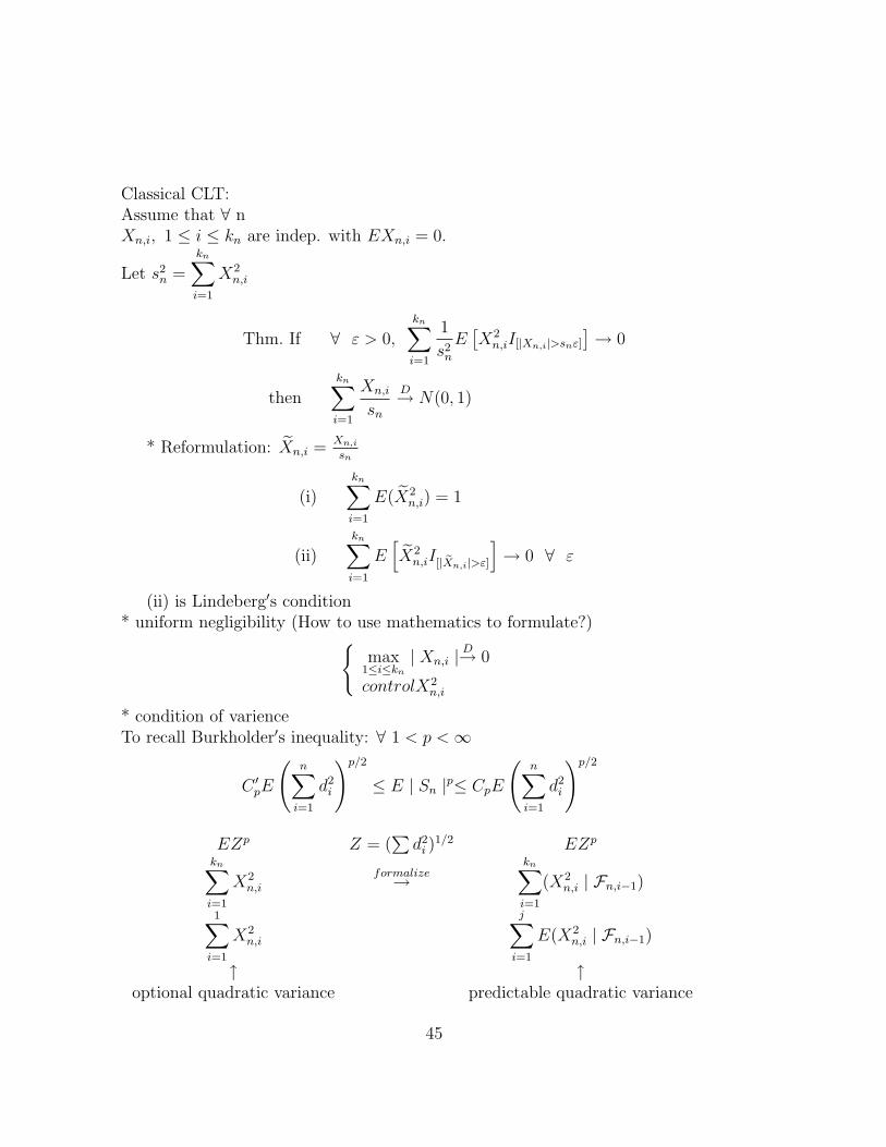
Classical CLT:Assume that ∀ nXn,i, 1 ≤ i ≤ kn are indep. with EXn,i = 0.
Let s2n =
kn∑i=1
X2n,i
Thm. If ∀ ε > 0,kn∑i=1
1
s2n
E[X2n,iI[|Xn,i|>snε]
]→ 0
thenkn∑i=1
Xn,i
sn
D→ N(0, 1)
* Reformulation: Xn,i =Xn,isn
(i)kn∑i=1
E(X2n,i) = 1
(ii)kn∑i=1
E[X2n,iI[|Xn,i|>ε]
]→ 0 ∀ ε
(ii) is Lindeberg′s condition* uniform negligibility (How to use mathematics to formulate?)
max1≤i≤kn
| Xn,i |D→ 0
controlX2n,i
* condition of varienceTo recall Burkholder′s inequality: ∀ 1 < p <∞
C ′pE
(n∑i=1
d2i
)p/2
≤ E | Sn |p≤ CpE
(n∑i=1
d2i
)p/2
EZp Z = (∑d2i )
1/2 EZp
kn∑i=1
X2n,i
formalize→kn∑i=1
(X2n,i | Fn,i−1)
1∑i=1
X2n,i
j∑i=1
E(X2n,i | Fn,i−1)
↑ ↑optional quadratic variance predictable quadratic variance
45

Thm. ∀ n ≥ 1, Fn,j; 1 ≤ j ≤ kn < ∞ is a sequence of increasing σ-fields. LetSn,j =
j∑i=1
Xn,i, 1 ≤ j ≤ kn
be Fn,j-adaptive.
Define
X∗n = max
1≤i≤kn| Xn,i |,
U2n,j =
j∑i=1
X2n,i, 1 ≤ j ≤ kn
Assume that
(i) U2n = U2
n,kn =kn∑i=1
X2n,i
D→ Co,where Co > 0 is a constant.
(ii) X∗n
D→ 0
(iii) supn≥1
E(X∗n)
2 <∞
(iv)kn∑j=1
EXn,j | Fn,j−1D→ 0 and
kn∑j=1
E2Xn,j | Fn,j−1D→ 0
Then
Sn =kn∑i=1
Xn,iD→ N(0, Co)
= Sn,kn
Remark:Xn,j, 1 ≤ j ≤ kn can be defined on different probability space for differentn.Step 1. Reduce the problem to the case
where Sn,j,Fn,j, 1 ≤ j ≤ kn is a martingale. Set
Xn,j = Xn,j − E(Xn,j | Fn,j−1) 1 ≤ j ≤ kn,Fn,o : trivial field
U2n =
kn∑j=1
X2n,j
X∗n = max
1≤j≤kn| Xn,j |
Sn =kn∑j=1
Xn,j
46
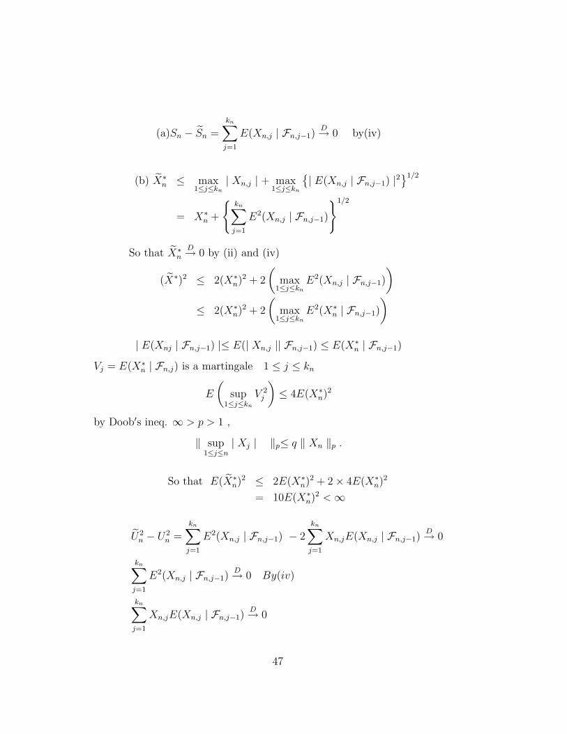
(a)Sn − Sn =kn∑j=1
E(Xn,j | Fn,j−1)D→ 0 by(iv)
(b) X∗n ≤ max
1≤j≤kn| Xn,j | + max
1≤j≤kn
| E(Xn,j | Fn,j−1) |2
1/2
= X∗n +
kn∑j=1
E2(Xn,j | Fn,j−1)
1/2
So that X∗n
D→ 0 by (ii) and (iv)
(X∗)2 ≤ 2(X∗n)
2 + 2
(max
1≤j≤knE2(Xn,j | Fn,j−1)
)≤ 2(X∗
n)2 + 2
(max
1≤j≤knE2(X∗
n | Fn,j−1)
)| E(Xnj | Fn,j−1) |≤ E(| Xn,j || Fn,j−1) ≤ E(X∗
n | Fn,j−1)
Vj = E(X∗n | Fn,j) is a martingale 1 ≤ j ≤ kn
E
(sup
1≤j≤knV 2j
)≤ 4E(X∗
n)2
by Doob′s ineq. ∞ > p > 1 ,
‖ sup1≤j≤n
| Xj | ‖p≤ q ‖ Xn ‖p .
So that E(X∗n)
2 ≤ 2E(X∗n)
2 + 2× 4E(X∗n)
2
= 10E(X∗n)
2 <∞
U2n − U2
n =kn∑j=1
E2(Xn,j | Fn,j−1) − 2kn∑j=1
Xn,jE(Xn,j | Fn,j−1)D→ 0
kn∑j=1
E2(Xn,j | Fn,j−1)D→ 0 By(iv)
kn∑j=1
Xn,jE(Xn,j | Fn,j−1)D→ 0
47

Because |kn∑i=1
Xn,jE(Xn,j | Fn,j−1) |≤
(kn∑j=1
X2n,j
)1/2( kn∑i=1
E2(Xnj | Fn,j−1)
)1/2
D→ 0
(kn∑j=1
X2n,j
)1/2
= (U2n)
1/2 D→ C1/2o(
kn∑i=1
E2(Xn,j | Fn,j−1)
)1/2
D→ 0
So that U2n
D→ Co
Thm. ∀n ≥ 1, Fn,j, 1 ≤ j ≤ kn < ∞ is a sequence of increasing σ-fields. Let
Sn,j =
j∑i=1
Xn,i, 1 ≤ j ≤ kn be Fn,j -martingale. Define X∗n = max
1≤i≤kn| Xn,i |
, U2n,j =
j∑i=1
X2n,i, 1 ≤ j ≤ kn
Assume that
(i) U2n = U2
n,kn =kn∑i=1
X2n,i
D→ Co, where Co > 0 is a constant
(ii) X∗n
D→ 0
(iii) supn≥1
E(X∗n)
2 <∞
Then
Sn =kn∑i=1
Xn,iD→ N(0, Co)
Step 2. Further Reduction. Define
τ =
infi : 1 ≤ i ≤ kn, U
2n,i > C , when U2
n > Ckn , when U2
n ≤ C
48

where C > Co
Define Xn,j = Xn,jI[τ≥j]
Sn =kn∑j=1
Xn,j =kn∑i=1
Xn,jI[τ≥j] =τ∑j=1
Xn,i
U2n,j =
j∑i=1
X2n,i,
X∗ = max1≤i≤kn
| Xn,j |
Un = U2n,kn =
τ∑j=1
X2n,j
P (Sn 6= Sn) ≤ P (U2n > C) → 0
⇒ It is sufficient to show that
SnD→ N(0, Co)
If C ≥ U2n then U2
n = U2n
If C < U2n then τ ≤ kn and
C < U2n =
τ−1∑i=1
X2n,j +X2
n,τ ≤ C + (X∗n)
2
So that U2n ∧ C ≤ U2
n ≤ (U2n ∧ C) +(X∗
n)2
↓ ↓ ↓ DCo ∧ C = Co Co ∧ C = Co 0
⇒ U2n
D→ Co
Clearly, X∗n ≤ X∗
n
Therefore, X∗n
D→ 0 by (ii) and
supn≥1
E(X∗n)
2 ≤ supn≥1
E(X∗n)
2 <∞
Step 3. E eiSn → e−co/2
Claim: This is sufficient to show SnD→ N(0, Co)
49

Reason : Step 3 ⇒ E eiSn → e−Co/2
Now replace Sn by t Sn. Using step 3 again, we obtain EeitSn → e−t2Co/2
(a) Expansioneix = (1 + ix)e(−x
2/2)+r(x) ,where | r(x) |≤| x |3 for | x |< 1
Because | x |< 1
⇒ ix = [log(1 + ix)]− x2/2 + r(x)
⇒ r(x) =x2
2+ ix− log(1 + ix)
=x2
2+ ix−
[∞∑j=1
(−1)j+1 (ix)j
j
]
=∞∑j=3
(−1)j(ix)j
j= −(ix)3
3+
(ix)4
4− · · ·
= x4a(x) + x3b(x)i
where a(x) =1
4− x2
6+x4
8− · · · < 1
4
b(x) =1
3− x2
5+x4
7· · · < 1
3
| r(x) | =√x8a2(x) + x6b2(x)
≤√x8
16+x6
9≤| x |3
√1
16+
1
9≤| x |3
eiSn =kn∏j=1
eiXn,j
=
[kn∏j=1
(1 + iXn,j)
]e
−
kn∑j=1
X2n,j/2 +
kn∑j=1
r(Xn,j)
def= Tne
−U2n/2+Rn
= (Tn − 1)e−Co/2 + (Tn − 1)[e−U
2n/2+Rn − e−Co/2
]+ e−U
2n/2+Rn
= In + IIn + IIIn
50
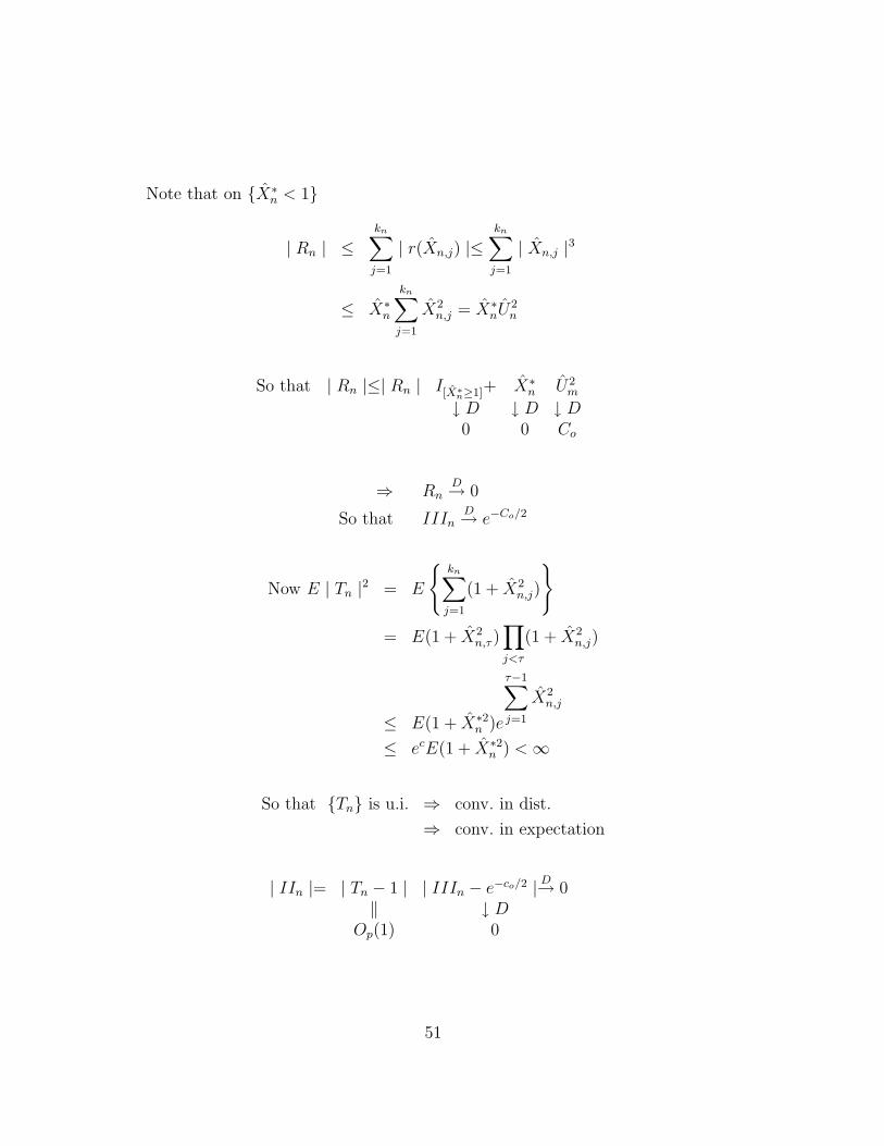
Note that on X∗n < 1
| Rn | ≤kn∑j=1
| r(Xn,j) |≤kn∑j=1
| Xn,j |3
≤ X∗n
kn∑j=1
X2n,j = X∗
nU2n
So that | Rn |≤| Rn | I[X∗n≥1]+ X∗n U2
m
↓ D ↓ D ↓ D0 0 Co
⇒ RnD→ 0
So that IIInD→ e−Co/2
Now E | Tn |2 = E
kn∑j=1
(1 + X2n,j)
= E(1 + X2
n,τ )∏j<τ
(1 + X2n,j)
≤ E(1 + X∗2n )e
τ−1∑j=1
X2n,j
≤ ecE(1 + X∗2n ) <∞
So that Tn is u.i. ⇒ conv. in dist.
⇒ conv. in expectation
| IIn |= | Tn − 1 | | IIIn − e−co/2 | D→ 0‖ ↓ D
Op(1) 0
51
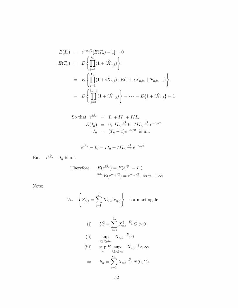
E(In) = e−co/2[E(Tn)− 1] = 0
E(Tn) = E
kn∏j=1
(1 + iXn,j)
= E
kn∏j=1
(1 + iXn,j) · E(1 + iXn,kn | Fn,kn−1)
= E
kn−1∏j=1
(1 + iXn,j)
= · · · = E1 + iXn,1 = 1
So that eiSn = In + IIn + IIIn
E(In) = 0, IInD→ 0, IIIn
D→ e−co/2
In = (Tn − 1)e−co/2 is u.i.
eiSn − In = IIn + IIInD→ e−co/2
But eiSn − In is u.i.
Therefore E(eiSn) = E(eiSn − In)u.i.→ E(e−co/2) = e−co/2, as n→∞
Note:
∀n
Sn,j =
j∑i=1
Xn,i,Fn,j
is a martingale
(i) U2n =
kn∑i=1
X2n,i
D→ C > 0
(ii) sup1≤i≤kn
| Xn,i |D→ 0
(iii) supnE sup
1≤i≤kn| Xn,i |2<∞
⇒ Sn =kn∑i=1
Xn,iD→ N(0, C)
52
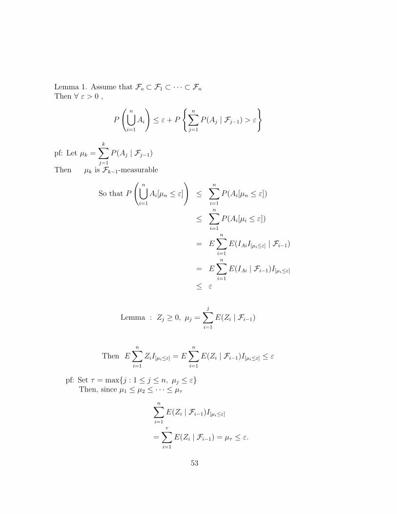
Lemma 1. Assume that Fo ⊂ F1 ⊂ · · · ⊂ FnThen ∀ ε > 0 ,
P
(n⋃i=1
Ai
)≤ ε+ P
n∑j=1
P (Aj | Fj−1) > ε
pf: Let µk =k∑j=1
P (Aj | Fj−1)
Then µk is Fk−1-measurable
So that P
(n⋃i=1
Ai[µn ≤ ε]
)≤
n∑i=1
P (Ai[µn ≤ ε])
≤n∑i=1
P (Ai[µi ≤ ε])
= E
n∑i=1
E(IAiI[µi≤ε] | Fi−1)
= En∑i=1
E(IAi | Fi−1)I[µi≤ε]
≤ ε
Lemma : Zj ≥ 0, µj =
j∑i=1
E(Zi | Fi−1)
Then En∑i=1
ZiI[µi≤ε] = En∑i=1
E(Zi | Fi−1)I[µi≤ε] ≤ ε
pf: Set τ = maxj : 1 ≤ j ≤ n, µj ≤ εThen, since µ1 ≤ µ2 ≤ · · · ≤ µτ
n∑i=1
E(Zi | Fi−1)I[µi≤ε]
=τ∑i=1
E(Zi | Fi−1) = µτ ≤ ε.
53
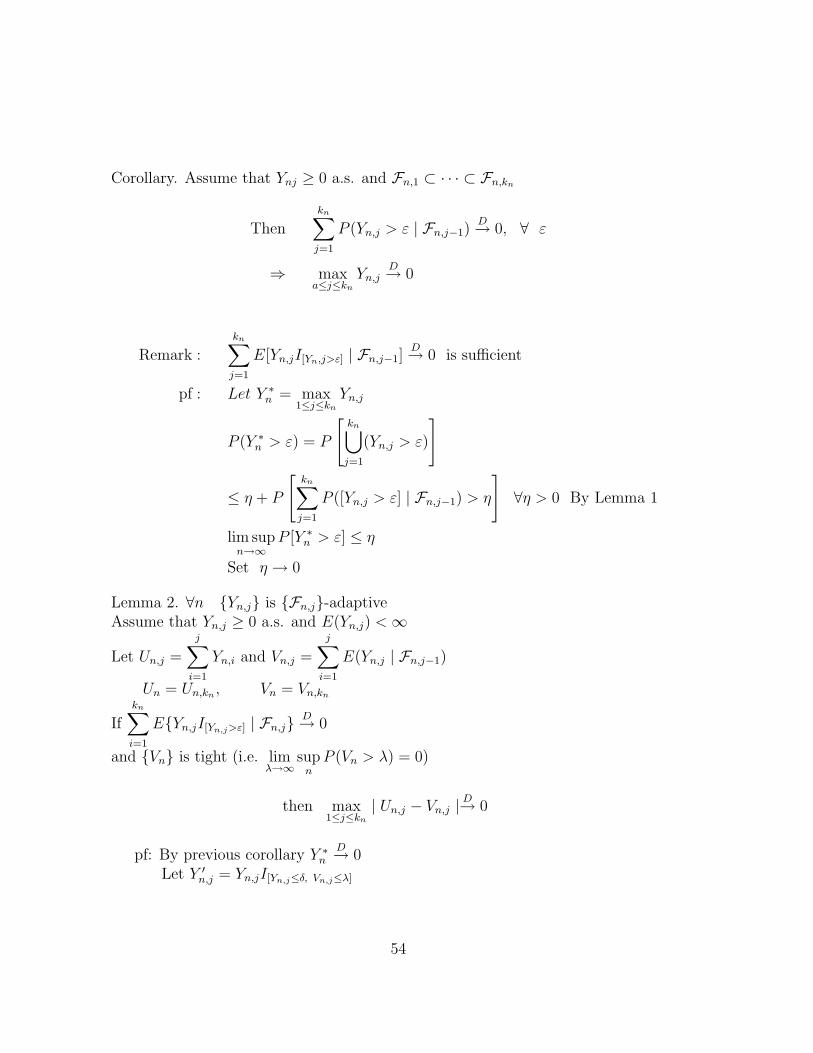
Corollary. Assume that Ynj ≥ 0 a.s. and Fn,1 ⊂ · · · ⊂ Fn,kn
Thenkn∑j=1
P (Yn,j > ε | Fn,j−1)D→ 0, ∀ ε
⇒ maxa≤j≤kn
Yn,jD→ 0
Remark :kn∑j=1
E[Yn,jI[Yn,j>ε] | Fn,j−1]D→ 0 is sufficient
pf : Let Y ∗n = max
1≤j≤knYn,j
P (Y ∗n > ε) = P
[kn⋃j=1
(Yn,j > ε)
]
≤ η + P
[kn∑j=1
P ([Yn,j > ε] | Fn,j−1) > η
]∀η > 0 By Lemma 1
lim supn→∞
P [Y ∗n > ε] ≤ η
Set η → 0
Lemma 2. ∀n Yn,j is Fn,j-adaptiveAssume that Yn,j ≥ 0 a.s. and E(Yn,j) <∞
Let Un,j =
j∑i=1
Yn,i and Vn,j =
j∑i=1
E(Yn,j | Fn,j−1)
Un = Un,kn , Vn = Vn,kn
Ifkn∑i=1
EYn,jI[Yn,j>ε] | Fn,jD→ 0
and Vn is tight (i.e. limλ→∞
supnP (Vn > λ) = 0)
then max1≤j≤kn
| Un,j − Vn,j |D→ 0
pf: By previous corollary Y ∗n
D→ 0Let Y ′
n,j = Yn,jI[Yn,j≤δ, Vn,j≤λ]
54
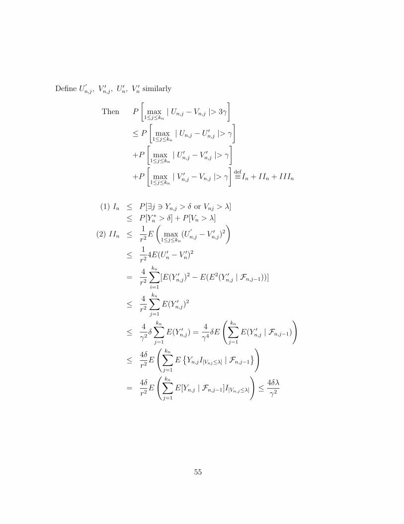
Define U′n,j, V
′n,j, U
′n, V
′n similarly
Then P
[max
1≤j≤kn| Un,j − Vn,j |> 3γ
]≤ P
[max
1≤j≤kn| Un,j − U ′
n,j |> γ
]+P
[max
1≤j≤kn| U ′
n,j − V ′n,j |> γ
]+P
[max
1≤j≤kn| V ′
n,j − Vn,j |> γ
]def≡In + IIn + IIIn
(1) In ≤ P [∃j 3 Yn,j > δ or Vnj > λ]
≤ P [Y ∗n > δ] + P [Vn > λ]
(2) IIn ≤ 1
r2E
(max
1≤j≤kn(U
′
n,j − V ′n,j)
2
)≤ 1
r24E(U ′
n − V ′n)
2
=4
r2
kn∑i=1
[E(Y ′n,j)
2 − E(E2(Y ′n,j | Fn,j−1))]
≤ 4
r2
kn∑j=1
E(Y ′n,j)
2
≤ 4
γ2δ
kn∑j=1
E(Y ′n,j) =
4
γ4δE
(kn∑j=1
E(Y ′n,j | Fn,j−1)
)
≤ 4δ
r2E
(kn∑j=1
EYn,jI[Vnj≤λ] | Fn,j−1
)
=4δ
r2E
(kn∑j=1
E[Yn,j | Fn,j−1]I[Vn,j≤λ]
)≤ 4δλ
γ2
55

(3) Note that max1≤j≤kn
| Vn,j − V ′n,j |
≤ max1≤j≤kn
|j∑i=1
(E(Yn,i | Fn,i−1)− E(Y ′n,i | Fn,i−1)) |
≤kn∑i=1
E(| Yn,i − Y ′n,i || Fn,i−1)
≤kn∑j=1
E(Yn,jI[Yn,j>δ or Vn,j>λ] | Fn,j−1)
≤kn∑j=1
E(Yn,jI[Yn,j>δ] | Fn,j−1) +kn∑j=1
E(Yn,jI[Vn,j>λ] | Fn,j−1)
≤kn∑j=1
E(Yn,jI[Yn,j>δ] | Fn,j−1) +kn∑j=1
E(Yn,j | Fn,j−1)I[Vn,j>λ]
≤kn∑j=1
E(Yn,jI[Yn,j>δ] | Fn,j−1) +kn∑j=1
E(Yn,j | Fn,j−1)I[Vn>λ]
≤kn∑j=1
E(Yn,jI[Yn,j>δ] | Fn,j−1) + VnI[Vn>λ]
IIIn ≤ P
[kn∑j=1
E(Yn,jI[Yn,j>δ] | Fn,j−1) >γ
2
]+P
[VnI[Vn>λ] >
γ
2
]≤ P
[kn∑j=1
E(Yn,jI[Yn,j>δ] | Fn,j−1) >γ
2
]+ P [Vn > λ]
So that lim supn→∞
P
[max
1≤j≤kn| Un,j − Vn,j |> 3γ
]≤ 2 sup
nP [Vn > λ] +
4δλ
γ2
Let λ→∞, δ = 1λ2 . The proof is completed.
56

Thm. ∀ n Sn,j =
j∑i=1
Xn,i,Fn,j is a martingale
If (i) V 2n =
kn∑i=1
E(X2n,i | Fn,i−1)
D→ C > 0
and (ii)kn∑i=1
E(X2n,iI[X2
n,i>ε]| Fn,i−1)
D→ 0 Conditional Lindeberg′s condition
then Sn =kn∑i=1
Xn,iD→ N(0, C)
pf: Set Yn,j = X2n,j
By (ii) and lemma 1, Y ∗n = max
1≤j≤knX2n,j
D→ 0
or max1≤j≤kn
| Xn,j |D→ 0
By (i), V 2n is tight.
Therefore by (ii) and lemma 2.
V 2n − U2
nD→ 0, So that U2
nD→ C by (i).
Now define X ′n,j = Xn,jI
j∑i=1
E(X2n,jI[X2
n,j>ε]| Fn,j−1) ≤ 1
Since P [Sn 6= S ′n] ≤ P
[kn∑j=1
E(X2n,jI[X2
n,j>ε]| Fn,j−1) > 1
]→ 0
So that it is sufficient to show that S ′nD→ N(0, C)
(a) max1≤j≤kn
| X ′n,j |≤ X∗
nD→ 0
(b) P [U2n 6= U
′2n ] ≤ P
[kn∑j=1
E(X2n,jI[X2
n,j>ε]| Fn,j−1) > 1
]→ 0
So that U′2n
D→ C
57
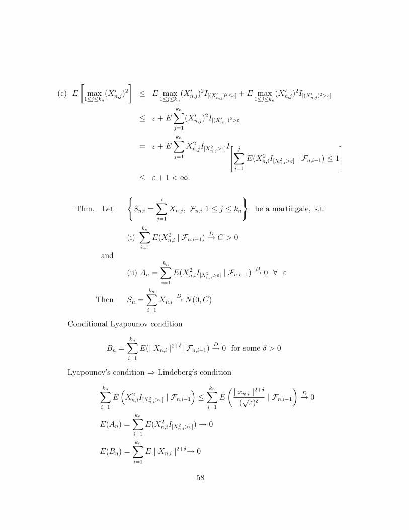
(c) E
[max
1≤j≤kn(X ′
n,j)2
]≤ E max
1≤j≤kn(X ′
n,j)2I[(X′n,j)2≤ε] + E max
1≤j≤kn(X ′
n,j)2I[(X′n,j)2>ε]
≤ ε+ E
kn∑j=1
(X ′n,j)
2I[(X′n,j)2>ε]
= ε+ E
kn∑j=1
X2n,jI[X2
n,j>ε]I
j∑i=1
E(X2n,iI[X2
n,i>ε]| Fn,i−1) ≤ 1
≤ ε+ 1 <∞.
Thm. Let
Sn,i =
i∑j=1
Xn,j, Fn,i 1 ≤ j ≤ kn
be a martingale, s.t.
(i)kn∑i=1
E(X2n,i | Fn,i−1)
D→ C > 0
and
(ii) An =kn∑i=1
E(X2n,iI[X2
n,i>ε]| Fn,i−1)
D→ 0 ∀ ε
Then Sn =kn∑i=1
Xn,iD→ N(0, C)
Conditional Lyapounov condition
Bn =kn∑i=1
E(| Xn,i |2+δ| Fn,i−1)D→ 0 for some δ > 0
Lyapounov′s condition ⇒ Lindeberg′s condition
kn∑i=1
E(X2n,iI[X2
n,i>ε]| Fn,i−1
)≤
kn∑i=1
E
(| xn,i |2+δ
(√ε)δ
| Fn,i−1
)D→ 0
E(An) =kn∑i=1
E(X2n,iI[X2
n,i>ε]) → 0
E(Bn) =kn∑i=1
E | Xn,i |2+δ→ 0
58
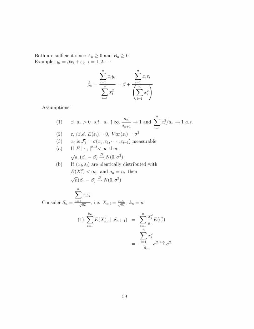
Both are sufficient since An ≥ 0 and Bn ≥ 0Example: yi = βxi + εi, i = 1, 2, · · ·
βn =
n∑i=1
xiyi
n∑i=1
x2i
= β +
n∑i=1
xiεi(n∑i=1
x2i
)
Assumptions:
(1) ∃ an > 0 s.t. an ↑ ∞,anan+1
→ 1 andn∑i=1
x2i /an → 1 a.s.
(2) εi i.i.d. E(εi) = 0, V ar(εi) = σ2
(3) xi is Fi = σ(xo, ε1, · · · , εi−1) measurable
(a) If E | ε1 |2+δ<∞ then√an(βn − β)
D→ N(0, σ2)
(b) If (xi, εi) are identically distributed with
E(X2i ) <∞, and an = n, then
√n(βn − β)
D→ N(0, σ2)
Consider Sn =
n∑i=1
xiεi
√an
, i.e. Xn,i = xiεi√an, kn = n
(1)kn∑i=1
E(X2n,i | Fn,i−1) =
n∑i=1
x2i
anE(ε2
i )
=
n∑i=1
x2i
anσ2 a.s.→ σ2
59
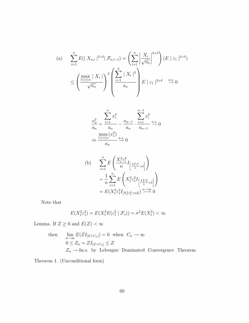
(a)n∑i=1
E(| Xn,i |2+δ| Fn,i−1) =
(n∑i=1
∣∣∣∣ Xi√an
∣∣∣∣2+δ)
(E | ε1 |2+δ)
≤
max1≤i≤n
| Xi |√an
δ
n∑i=1
| Xi |2
an
E | ε1 |2+δa.s.→ 0
x2n
an=
n∑i=1
x2i
an− an−1
an·
n−1∑i=1
x2i
an−1
a.s.→ 0
⇒max1≤i≤n
(x2i )
an
a.s.→ 0
(b)n∑i=1
E
(X2i ε
2i
nI[X2
iε2i
n>δ
])
=1
n
n∑i=1
E
(X2
1ε21I
[X2
1ε21
n>δ
])
= E(X21ε
21I[X2
1ε21>nδ]
)n→∞−→ 0
Note that
E(X21ε
21) = E(X2
1E(ε21 | Fo)) = σ2E(X2
1 ) <∞
Lemma. If Z ≥ 0 and E(Z) <∞
then limn→∞
E(ZI[Z>Cn]) = 0 when Cn →∞
0 ≤ Zn = ZI[Z>Cn] ≤ Z
Zn → 0a.s. by Lebesgue Dominated Convergence Theorem
Theorem 1. (Unconditional form)
60
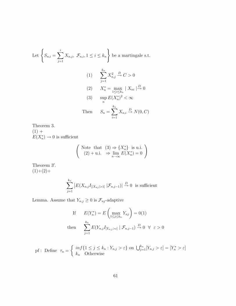
Let
Sn,i =
i∑j=1
Xn,j, Fn,i, 1 ≤ i ≤ kn
be a martingale s.t.
(1)kn∑j=1
X2n,j
D→ C > 0
(2) X∗n = max
1≤i≤kn| Xni |
D→ 0
(3) supnE(X∗
n)2 <∞
Then Sn =kn∑i=1
Xn,iD→ N(0, C)
Theorem 3.(1) +E(X∗
n) → 0 is sufficient(Note that (3) ⇒ X∗
n is u.i.(2) + u.i. ⇒ lim
n→∞E(X∗
n) = 0
)
Theorem 3′.(1)+(2)+
kn∑j=1
∣∣E(Xn,jI[|Xnj |>1] |Fn,j−1)|D→ 0 is sufficient
Lemma. Assume that Yn,j ≥ 0 is Fnj-adaptive
If E(Y ∗n ) = E
(max
1≤j≤knYnj
)= 0(1)
thenkn∑j=1
E(Yn,jI[Yn,j>ε] | Fn,j−1)D→ 0 ∀ ε > 0
pf : Define τn =
inf1 ≤ j ≤ kn : Yn,j > ε on
⋃knj=1[Yn,j > ε] = [Y ∗
n > ε]
kn Otherwise
61

∀δ > 0
P
kn∑j=1
E(Yn,jI[Yn,j>ε] | Fn,j−1) > δ
Fn,j−1−measurable
≤ Pτn < kn+ P
τn∑j=1
E(Yn,jI[Yn,j>ε] | Fn,j−1) > δ
≤ PY ∗n > ε+ P
kn∑j=1
I[τn≥j]E(Yn,jI[Yn,j>ε] | Fn,j−1) > δ
≤ PY ∗n > ε+ P
kn∑j=1
E(Yn,jI[τn≥j,Yn,j>ε] | Fn,j−1) > δ
≤ ε−1E(Y ∗n ) + δ−1E
(kn∑j=1
Yn,jI[τn≥j,Yn,j>ε]
)
≤ ε−1E(Y ∗n ) + δ−1E
(Y ∗n
kn∑j=1
I[τn≥j,Yn,j>ε]
)≤ ε−1E(Y ∗
n ) + δ−1E(Y ∗n ) → 0.
Corollary 1. Yn,j ≥ 0 is Fn,j-adaptive
If Y ∗n
D→ 0 thenkn∑j=1
P [Yn,j > ε | Fn,j−1]D→ 0, ∀ ε > 0
pf: Fix ε > 0
Let znj = I[Yn,j>ε] ≥ 0
z∗n = max1≤j≤kn
I[Yn,j>ε] = I[Y ∗n>ε]
E(z∗n) = P [Y ∗n > ε] = 0(1)
62

Thereforekn∑j=1
E(zn,jI[zn,j> 12] | Fn,j−1)
D→ 0
=kn∑j=1
E(I[Yn,j>ε]I[zn,j=1] | Fn,j−1)
=kn∑j=1
E(I[Yn,j>ε] | Fn,j−1)
=kn∑j=1
P (Yn,j > ε | Fn,j−1).
Corollary 2. Thm 3. is a corollary of Thm 3′.pf: Let Yn,j =| Xn,j |Then E(Y ∗
n ) = E(X∗n) → 0
So thatkn∑j=1
E(| Xn,j | I[|Xn,j |>ε] | Fn,j−1)D→ 0.
Corollary 3.If (1) Yn,j ≥ 0 is Fn,j-adaptive(2) | Yn,j |≤ C ∀ n, j
(3) Y ∗n
D→ 0
thenkn∑j=1
E(Y 2n,jI[Y 2
n,j>ε]| Fn,j−1)
D→ 0
pf:kn∑j=1
E(Y 2n,jI[Y 2
n,j>ε]| Fn,j−1)
≤ C2∑kn
j=1 P [Yn,j >√ε | Fn,j−1]
D→ 0 by (3) and Corollary 1.kn∑j=1
E(Yn,jI[Yn,j>ε] | Fn,j−1)D→ 0
Vn =∑kn
j=1E(Yn,j | Fn,j−1) is tight ⇒|kn∑j=1
Yn,j − Vn |D→ 0
63

pf. of Theorem 3′
Sn =kn∑i=1
Xn,i
=kn∑i=1
Xn,iI[|Xn,i|≤1] +kn∑i=1
Xn,iI[|Xn,i|>1]
Let Xn,i = Xn,iI[Xn,i|≤1]
Note thatP [Xn,j 6= Xn,j, for some 1 ≤ j ≤ kn]≤ P [X∗
n > 1] → 0 by (2)
So that Sn − SnD→ 0
and (1) giveskn∑j=1
X2n,j
D→ C
Xn,j = Xn,j − E(Xn,j | Fn,j−1)
Sn − Sn =kn∑j=1
E(Xn,jI[|Xn,j |≤1] | Fn,j−1)
= −kn∑j=1
E(Xn,jI[|Xn,j |>1] | Fn,j−1) By martingale properties.
So that | Sn − Sn | ≤kn∑j=1
| E(Xn,jI[|Xn,j |>1] | Fn,j−1) |D→ 0
Observe that
| Xn,j |≤ 1 ⇒| Xn,j |≤ 2
So that supnE(X∗
n) ≤ 2 [(3) is satisfied]
64

X∗n = max
1≤j≤n| Xn,j − E(Xn,j | Fn,j−1) |
≤ max1≤j≤n
| Xn,j | + max1≤j≤n
| E(Xn,jI[|Xn,j |>1] | Fn,j−1) |
≤ max1≤j≤n
| Xnj | +kn∑j=1
| E(Xn,jI[|Xn,j |>1] | Fn,j−1) |∣∣∣∣∣kn∑j=1
X2
n,j −kn∑j=1
X2n,j
∣∣∣∣∣=
∣∣∣∣∣−2kn∑j=1
Xn,jE(Xn,j | Fn,j−1) +kn∑j=1
E2(Xn,j | Fn,j−1)
∣∣∣∣∣≤ 2
∣∣∣∣∣kn∑j=1
Xn,jE(Xn,jI[|Xn,j |>1] | Fn,j−1)
∣∣∣∣∣+kn∑j=1
E2(Xn,jI[|Xn,j |>1] | Fn,j−1)
≤ 2
(kn∑j=1
X2n,j
)1/2( kn∑j=1
E2(Xn,jI[|Xn,j |>1] | Fn,j−1)
)1/2
+kn∑j=1
E2(Xn,jI[|Xn,j |>1] | Fn,j−1)
It is sufficient to show
kn∑j=1
| E(Xn,jI[|Xn,j |>1] | Fn,j−1) |2D→ 0 (By the assumption ∀ 0 < δ < 1)
kn∑j=1
| E(Xn,jI[|Xn,j |>1] | Fn,j−1) |≤
kn∑j=1
| E(Xn,jI[|Xn,j |>1] | Fn,j−1) |
2
D→ 0
65

Homework: Assume that Xn,j is Fnj-measurable
(1)kn∑j=1
E(X2n,jI[X2
n,j>ε]| Fn,j−1)
D→ 0
(2)kn∑j=1
E(Xn,j | Fn,j−1)D→ 0
(3)kn∑j=1
E(X2n,j | Fn,j−1)− E2(Xn,j | Fn,j−1)
D→ C > 0
Then Sn =kn∑j=1
Xn,jD→ N(0, C)
Exponential Inequality:Theorem 1 (Bennett′ inequality):Assume that Xn is a martingale difference with respect to Fn and τ is an Fn-stopping time (with possible value ∞). Let σ2
n = E(X2n | Fn−1) for n ≥ 1. Assume
that ∃ positive constants U and V such that Xn ≤ U a.s. for n ≥ 1 andτ∑i=1 σ
2i ≤ V
a.s., Then ∀ λ > 0
P
τ∑i=1
Xi ≥ λ
≤ exp
[−1
2λ2V −1ψ(4λV −1)
]where ψ(λ) = (2/λ2)[(1 + λ)log(1 + λ)− λ], ψ(0) = 1.Note:
(i)n∑i=1
Xi/√n =⇒ 1√
2π
∫ ∞
λ
e−x2
2 dx ∼ 1√2π
1
λe−
λ2
2 .
(ii) Prokhorov′s “arcsinh” inequality:Its upper bound is
h = exp
[−1
2λ(2υ)−1arcsinh(υλ(2V )−1
]where υλV −1 ≈ 0, arcsinh[υλ(2V )−1] ∼= υλ(2V )−1
h ∼= exp
[−1
2λ(2υ)−1υλ(2V )−1
]= exp
[− λ2
8V
]66

Reference: (i) Annals probability (1985).Johson, Schechtman, and Zin.
(ii) Journal of theoretical probalility (1989) (Levental).Corollary:(Bernsteins in equality).
P (τ∑i=1
Xi ≥ λ) ≤ exp
[−1
2λ2/(V +
1
3υλ)
]proof:
By ψ(λ) ≥ (1 +λ
3)−1, ∀ λ > 0.
idea:(i) Note that on (τ = ∞)
since∞∑i=1
E(X2i | Fi−1) =
τ∑i=1
σ2i ≤ V a.s.
τ∑i=1
Xi coverges a.s. on(τ = ∞).
(By Chow′s Theorem).(ii) We can replace
P
τ∑i=1
Xi ≥ λ
by P
τ∑i=1
Xi > λ
since λ > 0, δ > 0.
P
τ∑i=1
Xi > λ+ δ
≤ exp
[−1
2(λ+ δ)2V −1ψ(υ(λ+ δ)V −1
]
Let δ ↓ 0. Left = P
τ∑i=1
Xi ≥ λ
right = exp
[−1
2λ2V −1ψ(υλV −1)
]
67
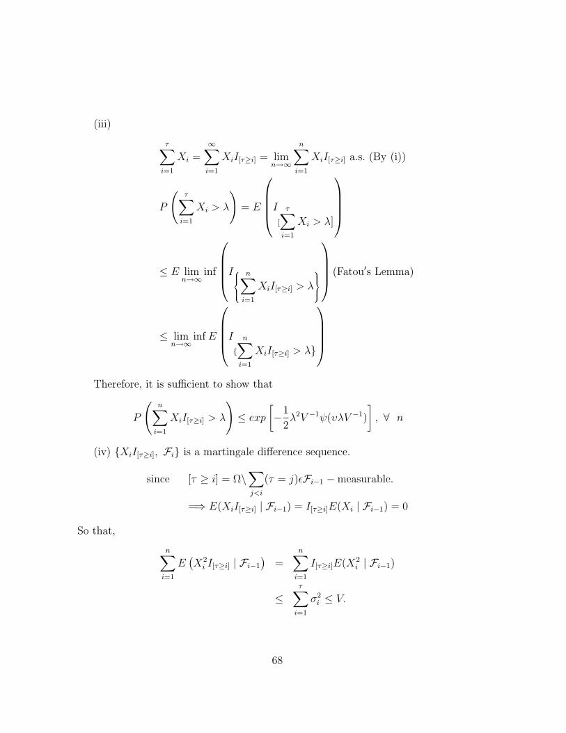
(iii)
τ∑i=1
Xi =∞∑i=1
XiI[τ≥i] = limn→∞
n∑i=1
XiI[τ≥i] a.s. (By (i))
P
(τ∑i=1
Xi > λ
)= E
I[
τ∑i=1
Xi > λ]
≤ E limn→∞
inf
In∑i=1
XiI[τ≥i] > λ
(Fatou′s Lemma)
≤ limn→∞
inf E
I
n∑i=1
XiI[τ≥i] > λ
Therefore, it is sufficient to show that
P
(n∑i=1
XiI[τ≥i] > λ
)≤ exp
[−1
2λ2V −1ψ(υλV −1)
], ∀ n
(iv) XiI[τ≥i], Fi is a martingale difference sequence.
since [τ ≥ i] = Ω\∑j<i
(τ = j)εFi−1 −measurable.
=⇒ E(XiI[τ≥i] | Fi−1) = I[τ≥i]E(Xi | Fi−1) = 0
So that,
n∑i=1
E(X2i I[τ≥i] | Fi−1
)=
n∑i=1
I[τ≥i]E(X2i | Fi−1)
≤τ∑i=1
σ2i ≤ V.
68

and XiI[τ≥i] ≤ υ a.s.Proof: Let Yi = XiI[τ≥i].
E(etYi | Fi−1), t > 0 (etYi ≤ etυ)
= E
(1 + tYi +
∞∑j=2
tjY ji
j!| Fi−1
)
≤ 1 +∞∑j=2
tjE[Y 2i | Fi−1]
j!υj−2, Y j
i = Y 2i Y
j−2i ≤ Y 2
i υj−2
= 1 +∞∑j=2
tjI[τ≥i]j!
σ2i υ
j−2
= 1 +
(∞∑j=2
tjυj
j!υ2
)I[τ≥i]σ
2i
= 1 + g(t)I[τ≥i]σ2i ≤ eg(t)I[τ≥i]σ
2i ,
where
g(t) = (etυ − 1− tυ)/υ2, and∞∑j=2
tjυj
j!=
∞∑j=0
(υt)j
j!− 1− tυ = etυ − 1− tυ
Claim:
e
t
j∑i=1
Yi/e
j∑i=1
I[τ≥i]σ2i
g(t)
is a supermartingale.
69
proof:
E
et
n∑i=1
Yi − g(t)n∑i=1
I[τ≥i]σ2i
| Fn−1
= e
t
n−1∑i=1
Yi − g(t)n∑i=1
I[τ≥i]σ2i
E[etYn | Fn−1
]≤ e
t
n−1∑i=1
Yi − g(t)n−1∑i=1
I[τ≥i]σ2i
Ee
t
n∑i=1
Yi≤ Ee
t
n∑i=1
Yi· e
g(t)
V−n∑i=1
I[τ≥i]σ2i
= E
et
n∑i=1
Yi − g(t)n∑i=1
I[τ≥i]σ2i
eg(t)V
≤ eg(t)V
(since V −
n∑i=1
I[τ≥i]σ2i > 0
)
P
n∑i=1
Yi > λ
≤ e−λtE
(et
∑ni=1 Yi
)≤ e−λt · eg(t)V = e−λt+g(t)V , ∀ t > 0,
⇒
P
n∑i=1
Yi > λ
≤ e
inft>0
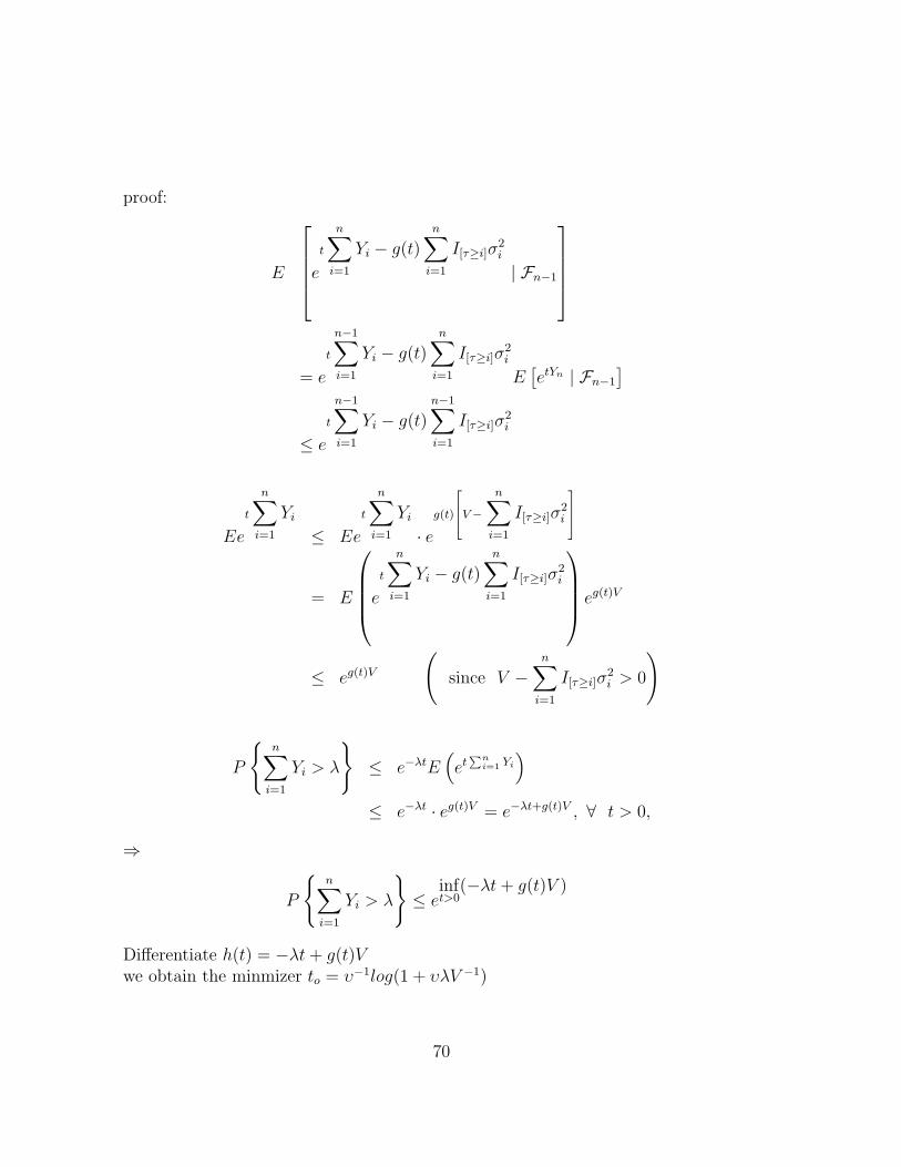
(−λt+ g(t)V )
Differentiate h(t) = −λt+ g(t)Vwe obtain the minmizer to = υ−1log(1 + υλV −1)
70
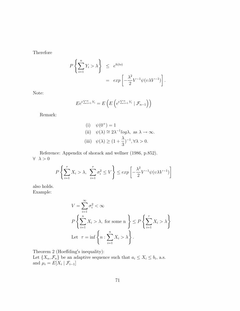
Therefore
P
n∑i=1
Yi > λ
≤ eh(to)
= exp
[−λ
2
2V −1ψ(υλV −1)
].
Note:
Eet∑ni=1 Yi = E
(E(et
∑ni=1 Yi | Fn−1
))Remark:
(i) ψ(0+) = 1
(ii) ψ(λ) ∼= 2λ−1logλ, as λ→∞.
(iii) ψ(λ) ≥ (1 +λ
3)−1,∀λ > 0.
Reference: Appendix of shorack and wellner (1986, p.852).∀ λ > 0
P
τ∑i=1
Xi > λ,τ∑i=1
σ2i ≤ V
≤ exp
[−λ
2
2V −1ψ(υλV −1)
]also holds.Example:
V =∞∑i=1
σ2i <∞
P
n∑i=1
Xi > λ, for some n
≤ P
τ∑i=1
Xi > λ
Let τ = inf
n :
n∑i=1
Xi > λ
.
Theorem 2 (Hoeffding′s inequality):Let Xn,Fn be an adaptive sequence such that ai ≤ Xi ≤ bi, a.s.and µi = E[Xi | Fi−1]
71

Then ∀ λ > 0,
P
n∑i=1
Xi −n∑i−1
µi ≥ λ
≤ exp
[− 2λ2∑n
i=1(bi − ai)2
]or P
Xn − µn ≥ λ
≤ exp
[− 2n2λ2∑n
i=1(bi − ai)2
]proof: By convexity of etx, (t > 0)
etXi ≤ bi −Xi
bi − aietai +
Xi − aibi − ai
etbi
E(et(Xi−µi) | Fi−1
)≤ bi − µi
bi − aiet(ai−µi) +
µi − aibi − ai
et(bi−µi)
= eL(hi)
where L(hi) = −hiPi + `n(1− Pi + Piehi)
hi = t(bi − ai), Pi =µi − aibi − ai
L(hi) = `n[(
1− Pi)et(ai−µi) + Pie
t(bi−µi))]
= `n[et(ai−µi)
((1− Pi) + Pie
t(bi−ai))]
L′(hi) = −Pi + Pi/[(1− Pi)e
−hi + Pi]
L′′(hi) =Pi(1− Pi)e
−hi
[(1− Pi)e−hi + Pi]2= ui(1− ui)
where 0 ≤ ui = Pi/[(1− Pi)e−hi + Pi] ≤ 1
L(hi) = L(0) + L′(0)hi +1
2L′′(h∗i )h
2i
≤ L(0) +1
2L′(0)hi +
1
8h2i
L(hi) ≤ h2i /8 ≤ t2(bi − ai)
2/8
So that E(et(Xi−µi)) ≤ exp
[t2(bi − ai)
2
8
]72
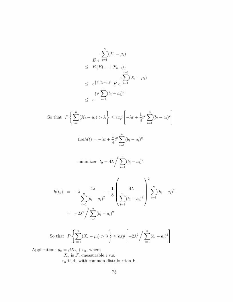
E e
t
n∑i=1
(Xi − µi)
≤ EE(· · · | Fn−1)
≤ e18t2(bi−ai)2 E e
t
n−1∑i=1
(Xi − µi)
≤ e
18t2
n∑i=1
(bi − ai)2
So that P
n∑i=1
(Xi − µi) > λ
≤ exp
[−λt+
1
8t2
n∑i=1
(bi − ai)2
]
Leth(t) = −λt+1
8t2
n∑i=1
(bi − ai)2
minimizer t0 = 4λ
/ n∑i=1
(bi − ai)2
h(t0) = −λ 4λn∑i=1
(bi − ai)2
+1
8
4λn∑i=1
(bi − ai)2
2
n∑i=1
(bi − ai)2
= −2λ2
/ n∑i=1
(bi − ai)2
So that P
n∑i=1
(Xi − µi) > λ
≤ exp
[−2λ2
/ n∑i=1
(bi − ai)2
]
Application: yn = βXn + εn, whereXn is Fn-measurable r.v.s.εn i.i.d. with common distriburtion F.
73

εn is independent of Fn−1 ⊃ σ(ε1, · · · , εn)Eεn = 0, 0 < V ar(εn) = σ2 <∞ .
Question : Test F = Fo (Ho)Example : AR(1) process
yn = βyn−1 + εn, yoεFo −measurable
Fn(u) =1
n
n∑i=1
I[yi−βnxi≤u],
where βn an estimator of β based on (y1, x1), · · · , (yn, xn).
idea : Fn(u) ∼= Fn(u) =1
n
n∑i=1
I[εi≤u], if βnxi ∼= βxi
supu| Fn(u)− F0(u) |
P→ 0
√n sup
u| Fn(u)− F0(u) |
D→ sup0≤t≤1
| oω (t) |, (Under Ho)
whereoω (t) is the Brownian Bridge which is defined by
oω (t) = w(t)− tw(1) and
w(t) is the Brownian Motion(i) w(ti)− w(si) are independent,∀ 0 = s0 ≤ t0 ≤ s1 ≤ t1 ≤ · · · ≤ sn ≤ tn(ii) w(t)− w(s) = N(0, t− s)(iii) w(0) = 0If the εn are independent and have a cemmon distribution function F (t). Then forlarge n,Fn(t, w) → F (t).Glivenko-Cantelli theoren:
sup0≤t≤1
| Fn(t)− F (t) |→ 0 a.s.
Fn(t) =1
n
n∑i=1
I[εi≤t]
Basic Theorem:If εi are i.i.d. U(0, 1).Then
αn(t) =1√n
(n∑i=1
[I[εi≤t] − F (t)
])D→ oω (t) in D− space.
74

Wish :√n sup
u| Fn(u)− Fn(u) |
P→ 0 (In general, it is wrong)
√n sup
u| Fn(u)− Fn(u) |
D→ sup0≤t≤1
| oω (t) |
Reject if√n sup
u| Fn(u)− Fn(u) |> Cα
Compare:
(i)√n sup
u| Fn(u)−
1
n
n∑i=1
F (u+ (βn − β)xi)− Fn(u) + F (u) | P→ 0 (right)
(ii)√n sup
u| [Fn(u)− F (u)]− [Fn(u)− F (u)] | P→ 0 (It is wrong, in general)
Fn(u) =1
n
n∑i=1
I[yi−βnxi≤u]
=1
n
n∑i=1
I[εi≤u+(βn−β)xi]
F (c xi + u)
= E(I[εi≤c xi+u] | Fi−1)
(If C is constant, we can use the exponential bound).√n(Fn(u)− F (u))
=√n(Fn(u)−
1
n
n∑i=1
F (·)− Fn(u) + F (u)) · · · (1)
+√n
(1
n
n∑i=1
F (·)− F (u)
)· · · (2)
+√n(Fn(u)− F (u)) · · · (3)
In fact, tell us:
1√n
n∑i=1
[F (u+ (βn − β)xi)− F (u)]
∼=1√n
n∑i=1
F ′(u)(βn − β)xi
= F ′(u)
(1√n
n∑i=1
xi
)(βn − β) does not converge to zero.
75

Example:
yi = βxi + εi, xi = 1, βn − β = εn(1√n
n∑i=1
xi
)(βn − β) =
√n(εn)
D→ N(0, 1)
wish:(1) → 0p(1)(2) → 0, and
known (3)D→ o
W(t), 0 ≤ t ≤ 1
Classical result: υ(0, 1) = FDefine:αn(t) =
√n(Fn(t)− t)
Oscillation modulus:
Wn(δ) = sup|t−u|≤δ
| αn(t)− αn(u) |
Lemma:∀ ε > 0, ∀ η > 0, ∃ δ and N 3 n ≥ N, PWn(δ) ≥ ε ≤ η.Reference:Billingsley, (1968)Convergence of probability measures. (Book).Papers:(i) W. Stute (1982, 1984). Ann. Prob. p.86-107, p.361-379.(ii) The Oscillation behavior of empirical process.: The Multivariate case.Key idea:• If (βn − β) ∼= C and u fixed. Then
1√n
n∑i=1
[I(εi≤Cxi+u) − F (Cxi + u)− I[εi≤u] + F (u)
]
Byn∑i=1
Yi, (Yi | Fi−1) ∼ b(1, Pi) and exponential bound. Pi ∈ Fi−1 -measurable.
• Lemma: If ‖ F ′∞ ‖, Then
√n sup
u|
n∑i=1
I[εi≤u+δni] − F (u+ δni)− I[εi≤u] + F (u) |
P→ 0, if δn = op(1√n
)
76
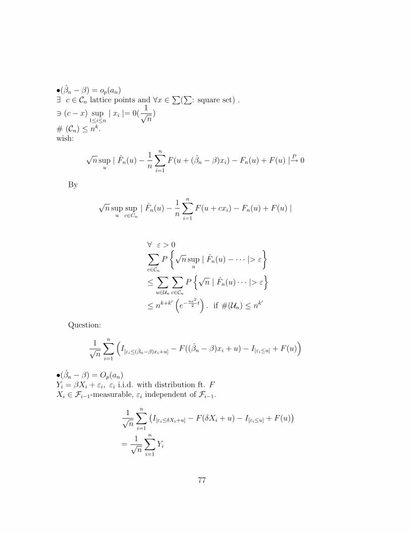
•(βn − β) = op(an)∃ c ∈ Cn lattice points and ∀x ∈
∑(∑
: square set) .
3 (c− x) sup1≤i≤n
| xi |= 0(1√n
)
# (Cn) ≤ nk.wish:
√n sup
u| Fn(u)−
1
n
n∑i=1
F (u+ (βn − β)xi)− Fn(u) + F (u) | P→ 0
By
√n sup
usupc∈Cn
| Fn(u)−1
n
n∑i=1
F (u+ cxi)− Fn(u) + F (u) |
∀ ε > 0∑c∈Cn
P
√n sup
u| Fn(u)− · · · |> ε
≤∑u∈Un
∑c∈Cn
P√
n | Fn(u) · · · |> ε
≤ nk+k′(e−
nε2
2t). if #(Un) ≤ nk
′
Question:
1√n
n∑i=1
(I[εi≤(βn−β)xi+u]
− F ((βn − β)xi + u)− I[εi≤u] + F (u))
•(βn − β) = Op(an)Yi = βXi + εi, εi i.i.d. with distribution ft. FXi ∈ Fi−1-measurable, εi independent of Fi−1.
1√n
n∑i=1
(I[εi≤δXi+u] − F (δXi + u)− I[εi≤u] + F (u)
)=
1√n
n∑i=1
Yi
77

(a) E[Yi | Fi−1] =
∫[ε≤δXi+u]
dF (ε)− F (δXi + u)−∫
[ε≤u]dF (ε) + F (u)
= 0
(b) − 1 ≤ yi ≤ 1
Hoeffding′s inequality: (not good)Yi,Fi is a martingale difference.
−1 = ai ≤ Yi ≤ bi = 1
PYn ≥ t ≤ exp
− 2n2t2
n∑i=1
(bi − ai)2
.
So that P
1√n
∣∣∣∣∣n∑i=1
Yi
∣∣∣∣∣ ≥ λ
≤ 2e−
2n2 λ2n
2n = 2exp[−λ2]
— It can′t reflect the true variance.Bennett′s inequality: (better)
Yi ≤ υ,τ∑i=1
E(Y 2i | Fi−1) ≤ V
P
τ∑i=1
Yi ≥ t
≤ exp
[− t2
2Vψ(UtV −1)
]
E(Y 2i | Fi−1) = | F (δXi + u)− F (u) || 1− (· · · ) |
≤ | F (δXi + u)− F (u) |≤ ‖ F ′ ‖∞| δ || Xi |
78
n∑i=1
E[Y 2i | Fi−1] ≤‖ F ′ ‖∞| δ |
n∑i−1
| xi |
βn − β =
n∑i=1
xiεi
n∑i=1
x2i
=
n∑i=1
xiεi(n∑i=1
x2i
) 12
1(n∑i=1
x2i
) 12
n∑i=1
x2i∼= a2
ncn
(βn − β)n∑i=1
| xi |≈ Op(1)
n∑i=1
| xi |(n∑i=1
x2i
) 12
≤ n12
(n∑i=1
x2i
) 12
take V =√nc, τ = n, υ = 1
P
| 1√
n
n∑i=1
Yi |> λ
≤ exp
−(√nλ)2
2√nc
ψ(√nλ/
√nc)
= exp
[−√nλ2
2cψ
(λ
c
)]Law of the iteratived logarithm:classical: Xn i.i.d., EXn = 0, 0 < V ar(Xn) = σ2 <∞
limn→∞
supSn√
2nloglogn= σ a.s.
(a) Zn = Sn
/√nσ
D∼ N(0, 1)
Sn = Zn
/√2loglogn
79

(b) if m and n very closeness.If Zm and Zn are very closeness.
E(ZmZn) =
E
(n∑i=1
Xi
)2
σ2√mn
=n
σ2√mn
==1
σ2
√n
m.
(c) nm
= 1c, c large enough.
n1 = c, n2 = c2, · · · , nk = ck
Zn1 , Zn2 , · · · , Znk ' i.i.d.N(0, 1).
(d) if Yi is i.i.d. N(0,1)
limn→∞
sup Yn
/√2logn = 1 a.s.
proof: ∀ ε > 0
PYn ≥ (1 + ε)√
2logn i.o. = 0
PYn ≥ (1− ε)√
2logn i.o. = 1
By Borel-Contelli lemma, we only have to check
∞∑n=1
PYn ≥ (1 + δ)√
2logn <∞
∼∞∑n=1
1
(1 + δ)√
2logne−
2(1+δ)2logn2
=∞∑n=1
1
(1 + δ)√
2logn
1
n(1+δ)2<∞ if δ > 0 .
(e) limn→∞
supZn,k√2logk
= 1 a.s.
nk = ck, loglognk = logk + loglogc.
(f) limk→∞
supSck√
ck · 2 · loglogck= 1 a.s.
80

(g) limn→∞
supSn
σ√
2nloglogn= 1 a.s.
Theorem A: Let Xi,Fi be a martingale difference such that | Xi |≤ υ a.s. and
s2n =
n∑i=1
E(X2i | Fi−1) →∞ a.s.
Then
limn→∞
supSn
sn(2loglogs2n)
12
≤ 1 a.s.
where
Sn =n∑i=1
Xi
Corollary:
limn→∞
infSn
sn(2loglogs2n)
12
≥ −1
and limn→∞
sup| Sn |
sn(2loglogs2n)
12
≤ 1 a.s.
proof: (theorem A)c > 1∀ k, let Tk = infn : s2
n+1 ≥ c2kSo that Tk is a stopping timeTk <∞ a.s. since s2
n →∞ a.s.Consider STk
S2Tk≤ c2k, S2
Tk
/c2k
a.s.→ 1.
Want to show:
(∗) PSTk > (1 + ε)ck
√2logk, i.o.
= 0(
⇒ limk→∞
sup (STk
/STk(2loglogs
2Tk
)12 )] ≤ 1 + ε a.s.
)81
By Bennett′s inequality, let
λ = (1 + ε)ck√
2logk, V = c2k, υ = υ
(∗) ≤∞∑k=1
exp
− λ2
2Vψ
(υλ
V
)
=∞∑k=1
exp
−(1 + ε)2c2kψ(υ(1+ε)ck
√2logk
c2k
)2logk
2c2k
≤ c′
∞∑k=1
exp[−(1 + ε′)2logk]
= c′∞∑k=1
1
k(1+ε′)2<∞
(Because (1 + ε)2logk · 1
1 + υ(1+ε)ck√
2logkc2k
≥ (1 + ε′)2logk)
∀ n, ∃ Tk, Tk+1, s.t. Tk ≤ n ≤ Tk+1
Sn = STk + Sn − STkSn
sn√
2loglogs2n
≤ STksn√
2loglogs2n
+Sn − STk
sn√
2loglogs2n
Given ε > 0 , choose c > 1So that ε2/(c2 − 1) > 1
n∑i=1
XiI[Tk<i≤Tk+1], Fn
is a martingale
supTk<n≤Tk+1
(Sn − STk) ≤ sup1≤n<∞
(n∑i=1
XiI[Tk<i≤Tk+1]
)
Since
Tk+1∑i=Tk+1
E(X2i | Fi−1) = S2
Tk+1− S2
Tk+1 ≤ c2(k+1) − c2k = c2k(c2 − 1).
Want to prove:
P supTk<n≤Tk+1
(Sn − STk) > εck√
2logk, i.o. = 0
pf : Def τ = infj :
j∑i=1
XiI[Tk<i≤Tk+1] > εck√
2logk
82
∞∑k=1
P
sup
Tk<n≤Tk+1
(Sn − STk) > εck√
2logk
=∞∑k=1
P
τ∑i=1
XiI[Tk<i≤Tk+1] > εck√
2logk
≤∞∑k=1
exp
[− ε2c2k2logk
2(c2 − 1)c2kψ
(υck
√2logk
(c2 − 1)c2k
)]≤
∞∑k=1
exp
[−ε
2logk
c2 − 1ψ
(υ√
2logkck
(c2 − 1)c2k
)]when k is large, [ε2/(c2 − 1)]ψ(·) ≥ 1 + δ, for some δ > 0.
≤ C ′∞∑k=1
exp[−(1 + δ) log k]
= C ′∞∑k=1
k−(1+δ) <∞.
Reference:
1. W. Stout: A martingale analysis of kolmogorov′s law of the iteratived logarithm.Z.W. Verw. Geb. 15, 279∼290, (1970).
2. D.A. Freedman, Ann. Prob. (1975), 3, 100-118. On Tail Probability ForMartingale.
Exponential Centering:X ∼ F, ∃ ϕ(t) = EetX
PX > µ
=
∫[x>µ]
dF (x) =
∫[x>µ]
ϕ(t)e−txetxdF (x)
ϕ(t)
= ϕ(t)
∫[x>µ]
e−txdG(x)
Under G, X have the mean=ψ′(t) and Variance=ψ′′(t).
where ψ(t) = logϕ(t), G(x) = etxdF (x)ϕ(t)
83
•∫xdG(x) =
∫xetx
ϕ(t)dF (x) =
ddt
∫etxdF
ϕ(t)=ϕ′(t)
ϕ(t)= [logϕ(t)]′
= ψ′(t)
Similarly, for∫x2dG(x).
So, Px > u
= ϕ(t)
∫[x>u]
e−txdG(x)
= ϕ(t)e−tψ′(t)
∫[x−ψ′(t)√ψ′′(t)
>u−ψ′−1(t)√
ψ′′(t)
] e−t(x−ψ′(t))dG(x)
= eψ(t)−tψ′(t)∫
[z>
u−ψ′(t)√ψ′′(t)
] e−t√ψ′′(t)zdH(z)
where H(z) = G(√ψ′′(t)z + ψ′(t)).
Example: X ∼ N(0, 1)
ϕ(t) = e−t2
2
ψ(t) = t2/2, ψ′(t) = t, ψ′′(t) = 1
PX > u = et2
2−t2∫
[z>u−t]e−tzdH(z)
H(z) ∼ N(0, 1)
Simulation: t = u
PX > u = e−u2
2
∫[z>0]
e−uzdH(z)
Exponential bound : t = u(1 + ε)
PX > u = e−u2
2(1+ε)2
∫[z>−εu]
e−u(1+ε)zdH(z)
≥ e−u2
2(1+ε)2
∫[0≥z>−εu]
e−u(1+ε)zdH(z)
Ref: R.B. Bahadur : Some limit theorems in statisties. SIAM.Lemma 1: If E[X | F ] = 0, E[X2 | F ] ≥ c > 0 and E[X4 | F ] ≤ d <∞
84

Then PX > 0 | F ∧ PX < 0 | F ≥ c2/4d.proof:
E[X | F ] = 0 ⇔ E[X+ | F ] = E[X− | F ]
E[X2 | F ] ≥ c ⇔ E[X+2 | F ] ≥ c
2or
E[X−2 | F ] ≥ c
2
Assume that:E(X+2 | F) ≥ c2
c
2≤ E(X+2 | F) = E[(X+)
23 · (X+4
)13 | F ] (Holder inequality)
≤ E23 (X+ | F)(E(X+)4)
13
So that (c
2)3 ≤ E2(X+ | F)E(X4 | F)
(c
2)3/d ≤ E2(X+ | F)
(c
2)
32/d
12 ≤ E(X+ | F) = E(X+I[X>0] | F)
≤ E14 (X4 | F)E
34 (I[X>0] | F) (Holder inequality)
≤ d14P
34X > 0 | F
(c
2)6/d2 ≤ dP 3X > 0 | F, implies
PX > 0 | F ≥ c2
4d
Similarly, E(X− | F) ≥( c
2)
32
d12
, and
PX < 0 | F ≥ c2/4d.
Lemma 2: Assume that εn,Fn is a martingale difference sequence such that
E
(n∑i=1
ε2i | Fo
)≥ c2 > 0.
n∑i=1
E(ε2i | Fi−1) ≤ c1 and sup
1≤i≤n| εi |≤M a.s.
85

Then there is a universal constant B s.t.
p
n∑i=1
εi < 0 | Fo
∧ P
n∑i=1
εi > 0 | Fo
≥ Bc22/(c
21 +M4)
proof: (i) Burkholder-Gundy-Davis
p > 0
E
[( sup1≤i≤n
|i∑
j=1
εj |P | Fo
]
≤ kE
( n∑j=1
E(ε2j | Fj−1)
)P2
| Fo
+kE
[(max1≤j≤n
| εi |P)| Fo
]use: If E(XIA) ≥ E(Y IA), ∀AεF , X ≥ 0, Y ≥ 0
Then E(X | F) ≥ E(Y | F) a.s.
p.f. : Let A = E(X | F) < E(Y | F)E(XIA − Y IA) = E[E(X | F)− E(Y | F)]IA
= E(XIA)− E(Y IA)
⇒ P (A) = 0.(ii) By a conditional version of B-G-D inequality take p=4.
E
∣∣∣∣∣n∑j=1
εj
∣∣∣∣∣4
| Fo
≤ kE
n∑i=1
(ε2i | Fi−1)
2
| Fo
+kE
(max1≤i≤n
| εi |4| Fo)
≤ kc21 + kM4 = k(c21 +M4)
86

By Lemma 1,
P
n∑i=1
εi > 0 | Fo
∧ P
n∑i=1
εi < 0 | Fo
≥ c22/4k(c
21 +M4) = Bc22/(c
21 +M4)
where B = 14k
use (i) E
(n∑i=1
εi | Fo
)= 0
(ii) E
( n∑i=1
εi
)2
| Fo
= E
(n∑i=1
ε2i | Fo
)≥ c2.
Similarly,
P
n∑i=1
εiε(−λ, 0) | Fo
∧ P
n∑i=1
εiε(0, λ) | Fo
≥ Bc22/(c
21 +M4)− c1/λ
2
(By Markov-inequality)
Let Sn =n∑i=1
Xi
Assumptions:(i) Xi,Fi is a martingale difference sequence.(ii) P| Xi |≤ d = 1, ∀ 1 ≤ i ≤ nNotations:
σ2i = E(X2
i | Fi−1), s2i =
i∑j=1
σ2j
g1(x) = x−1(ex − 1), g(x) = x−2(ex − 1− x)
Conditional Exponential Centering:
idea : PA | Fo = E(E(· · ·E(E(IA | Fn−1) | Fn−2) · · · | Fo))ϕi(t) = E[etXi | Fi−1], ψi(t) = logϕi(t)
Definition
F(t)i (x) = E[I[Xi≤x]e
tXi | Fi−1]/ψi(t)
87
So that PSn > λ | Fo
=
∫[Sn>λ]
· · ·∫ [ n∏
i=1
[ϕi(t)]
]e
−t
n∑i=1
xidF (t)
n · · · dF (t)1
=
∫[Sn>λ]
· · ·∫e
n∑i=1
[ψi(t)]
e
−t
n∑i=1
xidF (t)
n · · · dF (t)1
=
∫[Sn>λ]
· · ·∫e
n∑i=1
[ψi(t)− tψ′i(t)]
e
−t
n∑i=1
(xi − ψ′i(t))
dF (t)n · · · dF (t)
1
Under new measure,
E[Xi | Fi−1] = ψ′i(t).
V ar(Xi | Fi−1) = ψ′′i (t).
Goal : Compute PSn > λ | Fo= E(I[Sn>λ] | Fo)= E(E · · ·E(I[Sn>λ] | Fn−1) | Fn−2) · · · | Fo)
by d(t)Fi
=etXi
ϕi(t)dP [Xi ≤ x | Fi−1].
88
Now, if s2n ≤M, g(−td)− t2d2g2(−td)− g1(td) ≤ 0,
then PSn > λ | Fo
=
∫[Sn>λ]
· · ·∫ [ n∏
i=1
ϕi(t)
]e
−t
n∑i=1
xidF (t)
n · · · dF (t)1 ,∀t > 0
=
∫[Sn>λ]
· · ·∫e
n∑i=1
ψi(t)− t
n∑i=1
xidF (t)
n · · · dF (t)1
(∗∗) =
∫[Sn>λ]
· · ·∫e
n∑i=1
(ψi(t)− tψ′i(t))
e
−t
n∑i=1
(xi − ψ′i(t))
dF (t)n · · · dF (t)
1
under dF (t)n , · · · dF (t)
1 ,
E[Yi | Fi−1] =
∫ydF
(t)i (y) = E[Xie
tXi | Fi−1]
= [logϕi(t)]′ = ψ′i(t), and
V ar(Yi | Fi−1) = ψ′′i (t).
•ψ′i(t) = E(XietXi | Fi−1)
= E(Xi(etXi − 1) | Fi−1)
= E[tX2i
etXi − 1
tXi
| Fi−1]
= tE[X2i g1(tXi) | Fi−1], where g1(x) ↑ as x ↑ .
≤ tE[X2i g1(td) | Fi−1] ≤ tσ2
i g1(td).≥ tE[X2
i g1(−td) | Fi−1] ≥ tσ2i g1(−td).
Since g1(x) > 0,
(ex − 1
x≥ 0, ∀x
)ϕ′i(t) ≥ 0, There ϕi(t) ≥ ϕi(0) = 1
89
• • ϕi(t) = E[etXi | Fi−1]
= E[1 + tXi + t2X2i g(tXi) | Fi−1]
≤ 1 + t2σ2i g(td)
≥ 1 + t2σ2i g(−td)
• • •ψ′i(t) =ϕ′i(t)
ϕi(t)≤ tg1(td)σ
2i
≥ tg1(−td)σ2i
1+t2σ2i g(td)
So, ψi(t)− tψ′i(t) ≥ logϕi(t)− t2σ2i g1(td).
≥ log[1 + t2σ2i g(−td)]− t2σ2
i g1(td)
(1 + u ≥ eu−u2
, u ≥ 0; eu2
(1 + u) ≥ eu)
≥ t2σ2i g(−td)− t4σ4
i g2(−td)− t2g1(td)σ
2i
≥ t2σ2i g(−td)− t2d2g2(−td)− g1(td)
Because σ2i = E(X2
i | Fi−1) ≤ d2
, and
n∑i=1
(ψi(t)− tψ′i(t))
≥ t2s2ng(−td)− t2d2g2(−td)− g1(td)
Becausen∑i=1
σ2i = s2
n.
90
Thus,
(∗∗) ≥ et2M [g(−td)−t2d2g2(−td)−g1(td)]
·∫
[Sn>λ]
· · ·∫e
−t
n∑i=1
(xi − ψ′i(t))
dF (t)n · · · dF (t)
1 .([Sn > λ] = [Sn −
n∑i=1
ψ′i(t) > λ−n∑i=1
ψ′i(t)].
)
≥∫· · ·∫
[Sn−
∑ni=1 ψ
′i(t)≥λ−
tmg(−td)1+t2d2g(td)
] e−t
n∑i=1
(xi − ψ′i(t))
dF (t)
n · · · dF (t)n
·et2M [g(−td)−t2d2g2(−td)−g1(td)]
≥ et2M [g(−td)−t2d2g2(−td)−g1(td)]
·∫· · ·∫
[0≥Sn−
∑ni=1 ψ
′i(t)≥λ−
tmg(−td)1+t2d2g(td)
] 1dF (t)n · · · dF (t)
1 .
• • • • ϕ′′i (t) = E(X2i e
tXi | Fi−1)
≤ E(X2i e
td | Fi−1) = etdσ2i
≥ e−tdσ2i
ψ′′i (t) =ϕ′′i (t)
ϕi(t)− (ψ′i(t))
2
≤ ϕ′′i (t)/ϕi(t) ≤ ϕ′′i (t) ≤ etdσ2i
≥ e−tdσ2i
1 + t2σ2i g(td)
− t2g21(td)σ
4i
≥ σ2i e−tde−t
2σ2i g(td) − t2g2
1(td)σ4i
≥ σ2i [e
−td−t2d2g(td) − t2d2g21(td)].
So,n∑i=1
ψ′′i (t)
=
≤ s2
netd
≥ s2ne−td−t
2d2g(td) − t2d2g21(td)
91

Replace t by t/√M and λ by (1− r)
√Mt.
(∗ ∗ ∗) PSn > (1− r)√Mt | Fo
≥ et2g(−td/
√M)−(td/
√M)2g2(− td√
M)−g1( td√
M)
·∫· · ·∫[
0≥∑ni=1
(xi−ψ′i
(t√M
))≥(1−r)
√Mt−
m t√Mg(−td/
√M)
1+ t2Md2g2(td/
√M)
] dF (t/√M)
n · · · dF (t/√M)
1
Let εi = Xi − ψ′i(t/√M), | εi |≤
2d√M
(1)n∑i=1
E(ε2i | Fi−1) ≤
s2n
Me(td/
√M) ≤ etd/
√M = c1
(2) E
[n∑i=1
ε2i | Fo
]= E
[n∑i=1
(Xi − ψ′i(t/√M))2 | Fo
]
≥ M1
M− 2
td√Mg1
(td√M
)+m
M
t√Mg1(−
td√M
)/(1 +t2d2
Mg2(
td√M
))
Thus,
(∗ ∗ ∗) ≥ et2[g(td/
√M)−(td/
√M)2g2(−td/
√M)−g1(td/
√M)]
·
[M1
M− (2td/
√M)g1(td/
√M) + m
Mt√Mg(−td/
√M) ·B
e2td/√M + (2d/
√M)4
− etd/√M
t2[(1− r)− mMtg(−td/
√M)/(1 + t2d2
Mg2(td/
√M))]2
Let t→∞, and td/
√M → 0
Assume thatn∑i=1
E(X2i | Fo) ≥M1 > 0, and let M1/M → 1, m/M → 1,
m ≤n∑i=1
E(X2i | Fi−1) ≤M , and 1− (m/M) < r
ThenPSn > (1− r)
√Mt | Fo
≥ e−t2
2(1+0(1)) ·B(1 + 0(1))
In summary:
92

For each n, Xn,i, Fu,i, i = 1, 2, · · · , n is a martingale difference such that
(1) supn| Xn,i |≤ dn, dn increasing.
(2) mn ≤n∑i=1
E(X2n,i | Fn,(i−1)) ≤Mn,
n∑i=1
E(X2n,i | Fn,o) ≥Mn,1,
where mn/Mn → 1, Mn,1/Mn → 1
If tn →∞, and tndn/√Mn → 0
then
P
n∑i=1
Xn,i > (1− r)√Mntn | Fno
≥ e−
t2n2
(1+0(1)) · C(1 + 0(1))
Theorem: Assume that
Sn =
n∑i=1
Xi,Fn
is a martingale
such that sup1≤n<∞
| Xn |≤ d <∞ a.s.
Let σ2i = E(X2
i | Fi−1) and s2n =
n∑i=1
σ2i
If s2n →∞ a.s., then
limn→∞
sup Sn/(2s2nloglogs
2n)
1/2 = 1 a.s.
proof: (i) “≤ ” is already shown.(ii) To show “≥ 1”.
we only have to show that ∀ ε > 0, ∃ nk 3
PSnk > (1− ε)(2s2nkloglogs2
nk)1/2 i.o. = 1
Given c > 1, let τk = n : s2n+1 ≥ ck
τk is a stopping time, since
s2n+1 =
n+1∑i=1
E(X2i | Fi−1) is Fn measurable.
Note that
s2τk< ck, s2
τk+1≥ ck
93

(1) s2τk+1
− s2τk
≤ ck+1 −[s2τk+1 − σ2
τk+1
]≤ ck+1 − ck + d2
(2) s2τk+1
− s2τk
≥(s2τk+1+1 − σ2
τk+1+1
)− ck
≥ ck+1 − d2 − ck
By in summary,
Sτk+1− Sτk =
τk+1∑i=τk+1
Xi =∞∑i=1
XiI[τk<i≤τk+1]
PSτk+1− Sτk > (1− δ)(2s2
τk+1loglogs2
τk+1)1/2 | Fτk
≥ PSτk+1− Sτk > (1− δ)(2ck+1loglogck+1)1/2 | Fτk
(∗) = PSτk+1− Sτk > (1− r)(
1− δ
1− r)(2ck+1loglogck+1)1/2 | Fτk
let r = δ/2 and choose c so that
1− δ
1− δ/2<
√1− 1
c, implies
1− δ
1− r≤√
1− c−1 ≤√
1− c−1 +d2
ck+1
Mk = ck+1 − ck + d2, mk = ck+1 − d2 − ck
tk =(2loglogck+1)1/2
(1− c−1 + d2
ck+1 )1/2(1− δ
1− r)
< α(2loglogck+1)1/2, 0 < α < 1.
(∗) = PSτk+1− Sτk > (1− r)
√Mktk | Fτk
≥ e−t2k2
(1+0(1))B(1 + 0(1))
≥ B(1 + 0(1))e−α2loglogck+1(1+0(1))
≥ B(1 + 0(1))((k + 1)α2(1+0(1)))−1
So that,∞∑k=1
PSτk+1− Sτk > (1− r)
√Mktk | Fτk = ∞ a.s.
So that, PSτk+1− Sτk > (1− δ)(2s2
τk+1loglogs2
τk+1)1/2 i.o. | Fτk
= 1
94

But
Sτk(2s2
τk+1loglogs2
τk+1
)1/2=
Sτk(2s2
τkloglogs2
τk
)1/2 (s2τkloglog × s2
τk)1/2(
sτk+1loglog × s2
τk+1
)1/2
(s2τkloglogs2
τk)1/2(
s2τk+1
loglogs2τk+1
)1/2≤ (ckloglogck)1/2
((ck+1 − d2)loglogck+1)1/2
≤ (1/(c− d2/ck))1/2 → 0, as c→∞≤ δ (choose c so that)
So that, with c choosen,
limk→∞
sup Sτk+1/(2s2
τk+1loglogs2
τk+1)
≥ limk→∞
supSτk+1
− Sτk(2s2
τk+1loglog s2
τk+1)1/2
+ limk→∞
sup Sτk/(2s2τk+1
loglogs2τk+1
)1/2
≥ (1− δ) + (−1)δ = 1− 2δ
By limn→∞
sup(an + bn)
≥ limn→∞
sup an + limn→∞
inf bn.
History of L.I.L.:Step 1:
Xi i.i.d. PXi = 1 = PXi = −1 = 1/2
Sn =n∑i=1
Xi
s2n = n
(1913) Hausdorff: Sn = O(n12+ε) a.s.
(By moment and chebyshev′s inequality).(1914) Hardy-Littlewood:
Sn = O((n log n)1/2)
(By e−x2
2 or e−x/2)
95

(1922) Steinhauss:
limn→∞
sup Sn/(2nlogn)1/2 ≤ 1 a.s.
(1923) Khinchine:
Sn = O((n loglogn)1/2)
(1924) Khinchine:
limn→∞
sup Sn/(2n loglog n)1/2 = 1 a.s.
step 2:(1929) Kolmogorov:
Xi indep. r.v′.s EXi = 0, s2n =
n∑i=1
EX2i
(i) sup1≤k≤n
| Xk |≤ knsn
(loglogs2n)
1/2
(ii) kn → 0, s2n →∞.
Then
limn→∞
sup Sn/(2s2nloglogs
2n)
1/2 = 1 a.s.
(1937) Marcinkewicz and Zygmund:Given an example:
Sn =n∑i=1
ciεi, P (εi = −1) = P (εi = 1) =1
2,
εn i.i.d.
cn is choosen, so that kn → k > 0, | cn |≤knsn
(2 loglogs2n)
1/2.
They showed that
limn→∞
sup Sn/(2s2n loglogs
2n)
1/2 < 1 a.s.
(1941) Hartman and WitterXi i.i.d. EXi = 0, V ar(Xi) = σ2.
96
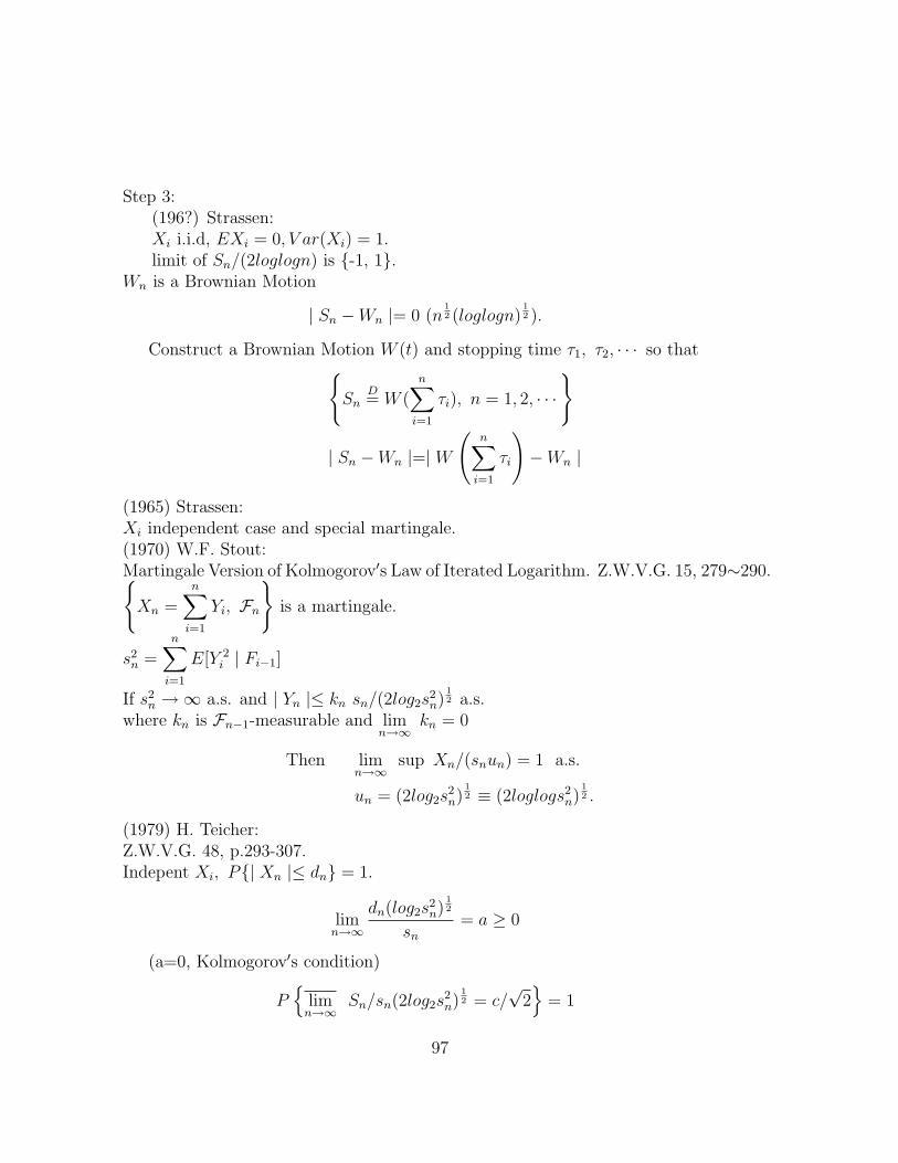
Step 3:(196?) Strassen:Xi i.i.d, EXi = 0, V ar(Xi) = 1.limit of Sn/(2loglogn) is -1, 1.
Wn is a Brownian Motion
| Sn −Wn |= 0 (n12 (loglogn)
12 ).
Construct a Brownian Motion W (t) and stopping time τ1, τ2, · · · so thatSn
D= W (
n∑i=1
τi), n = 1, 2, · · ·
| Sn −Wn |=| W
(n∑i=1
τi
)−Wn |
(1965) Strassen:Xi independent case and special martingale.(1970) W.F. Stout:Martingale Version of Kolmogorov′s Law of Iterated Logarithm. Z.W.V.G. 15, 279∼290.Xn =
n∑i=1
Yi, Fn
is a martingale.
s2n =
n∑i=1
E[Y 2i | Fi−1]
If s2n →∞ a.s. and | Yn |≤ kn sn/(2log2s
2n)
12 a.s.
where kn is Fn−1-measurable and limn→∞
kn = 0
Then limn→∞
sup Xn/(snun) = 1 a.s.
un = (2log2s2n)
12 ≡ (2loglogs2
n)12 .
(1979) H. Teicher:Z.W.V.G. 48, p.293-307.Indepent Xi, P| Xn |≤ dn = 1.
limn→∞
dn(log2s2n)
12
sn= a ≥ 0
(a=0, Kolmogorov′s condition)
P
limn→∞
Sn/sn(2log2s2n)
12 = c/
√2
= 1
97

where 0.3533/a ≤ c ≤ minb>0
[1
b+ bg(a, b)]
(1986) E. Fisher:Sankhya, Series A, 48, p.267∼ 272.Martingale Version:
limn→∞
sup kn < k. a.s.
implies limn→∞
supn∑i=1
Yi/sn(2log2s2n)
12 ≤ 1 + ε(k).
where ε(k) =
k/4, if 0 < k ≤ 1(3 + 2k2)/4k − 1, if k > 1.
This bound is not as good as Teicher′s bounds.Problems:
1. Do we have a martingale version of Teicher′s result?
2. M-Z. implies c/√
2 < 1.Teicher′s result does not imply this.How to interprate M-Z phenomenon?
3. Can we extend martingale′s result to the double arrays of martingale differencesSn?
Sn =∞∑−∞
ani εi.
Lai and Wei (1982). Annals prob. 10, 320∼ 335.
Papers:D. Freedman (1973). Annals probability, 1, 910∼925.Basic assumptions:
(i) Fo ⊂ F1 ⊂ · · · ⊂ Fn · · · (σ −fields)
(ii) Xn is Fn−measurable, n ≥ 1.
(iii) 0 ≤ Xn ≤ 1 a.s.
Sn =n∑i=1
Xi, Mi = E[Xi | Fi−1], Tn =n∑i=1
Mi.
98
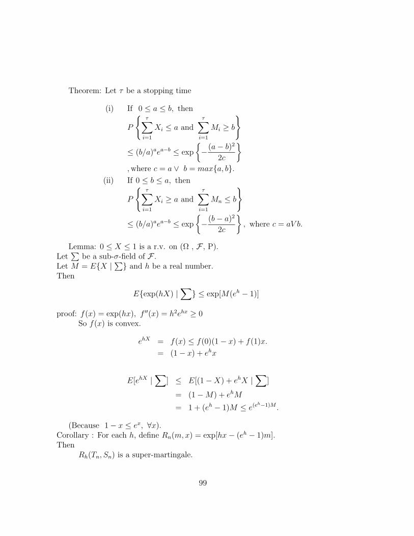
Theorem: Let τ be a stopping time
(i) If 0 ≤ a ≤ b, then
P
τ∑i=1
Xi ≤ a andτ∑i=1
Mi ≥ b
≤ (b/a)aea−b ≤ exp
−(a− b)2
2c
,where c = a ∨ b = maxa, b.
(ii) If 0 ≤ b ≤ a, then
P
τ∑i=1
Xi ≥ a andτ∑i=1
Mn ≤ b
≤ (b/a)aea−b ≤ exp
−(b− a)2
2c
, where c = aV b.
Lemma: 0 ≤ X ≤ 1 is a r.v. on (Ω , F , P).Let
∑be a sub-σ-field of F .
Let M = EX |∑ and h be a real number.
Then
Eexp(hX) |∑
≤ exp[M(eh − 1)]
proof: f(x) = exp(hx), f ′′(x) = h2ehx ≥ 0So f(x) is convex.
ehX = f(x) ≤ f(0)(1− x) + f(1)x.
= (1− x) + ehx
E[ehX |∑
] ≤ E[(1−X) + ehX |∑
]
= (1−M) + ehM
= 1 + (eh − 1)M ≤ e(eh−1)M .
(Because 1− x ≤ ex, ∀x).Corollary : For each h, define Rn(m,x) = exp[hx− (eh − 1)m].Then
Rh(Tn, Sn) is a super-martingale.
99

proof:
Rh(Tn, Sn) = Rh(Tn−1, Sn−1) exp[hXn − (eh − 1)Mn]
So E[Rh(Tn, Sn) | Fn−1]
≤ Rh(Tn−1, Sn−1)E[exp hXn | Fn−1] exp[−(eh − 1)Mn]
≤ Rh(Tn−1, Sn−1) (By lemma).
In the following, we use exp(∞) = ∞, exp(−∞) = 0, thenRh(m,x) is a continuous function on [0,∞]2 − (∞,∞).Lemma: Let τ be a stopping time.
G = Tτ <∞ or Sτ <∞
Then
∫G
Rh(Tτ , Sτ )dP ≤ 1.
proof: By the super-martingale property,∀ n, ERh(Tτ∧n, Sτ∧n) ≤ 1.
So that, 1 ≥ limn→∞
infE[Rh(Tτ∧n, Sτ∧n)]
≥ E[
limn→∞
infRh(Tτ∧n, Sτ∧n)]
(Fautou′s Lemma).
≥∫G
limn→∞
inf Rh(Tτ∧n, Sτ∧n)
=
∫G
Rh(Tτ , Sτ )dP.
proof of the theorem:
Let u(m,x) =
1, if m ≥ b and x ≤ a,∀ (m,x)ε[0,∞]2
0, o.w.
Qh(m,x) = exp[ha− (1− e−h)b] R−h(m,x),
∀ (m,x)ε[0,∞]2 − (∞,∞), ∀ h ≥ 0
100

Then
PSτ ≤ a and Tτ ≥ b
=
∫u(Tτ , Sτ )dP
=
∫G
(Tτ , Sτ )dP, G = Tτ <∞ or Sτ <∞
≤∫G
Qh(Tτ , Sτ )dP ( Qh ≥ u)
(Qh(m,x) = exp[−h(x− a) + (1− e−h)(m− b)] ≥ 1, if m ≥ b and x < a)
= Qh(0, 0)
∫G
R−h(Tτ , Sτ )dP
≤ Qh(0, 0)
So PSτ ≤ a and Tτ ≥ b ≤ infh≥0
Qh(0, 0)
= inf exp[ha− (1− e−h)b]
= exp
[infh≥0
[ha− (1− e−h)b
].
d/dh[ha− (1− e−h)b] = a− e−hb
minimum point ho satisfies eho = b/a
So that, minh≥0
Qh(0, 0) = exp(hoa) · exp[be−ho − b]
= (eho)a exp[(eho)−1b− b]
= (b/a)a exp[a
b· b− b]
So, PSτ ≤ a and Tτ ≥ b≤ (b/a)ae(a−b).
Another one: Let
u(m,x) =
1, if m ≤ b and x ≥ a0, o.w.
h ≥ 0, Qh(m,x) = exp[−ha+ (eh − 1)b]Rh(m,x)
G = Tτ <∞ and Sτ <∞, a > 0.
101

Lemma1 : a ≥ 0, b ≥ 0, c = a ∨ bThen (b/a)aea−b ≤ exp[−(a− b)2/2c]
Lemma1′: 0 < ε < 1, f(ε) = (
1
1− ε)1−εe−ε, g(ε) = (1− ε)eε.
we have
f(ε) < exp[−ε2/2] < 1 and
g(ε) < exp[−ε2/2] < 1.
proof : log f(ε) = −(1− ε) log(1− ε)− ε
(Because − log(1− x) = x+x2
2+x3
3+ · · · , 0 < x < 1).
= (1− ε)[ε+ε2
2+ε3
3+ · · · ]− ε
= [ε+ε2
2+ε3
3+ · · · ]− ε2 − ε2
2− · · · − ε
≤ −ε2/2
log g(ε) = log(1− ε) + ε
= −(ε+ε2
2+ε3
3+ · · · ) + ε
≤ −ε2/2
proof of Lemma 1:(i) a=b (trivial).(ii) case 1: 0 < a < b, let ε = (b− a)/b = 1− a/b.
(b/a)a ea−b = [(1− ε)−1](1−ε)beb (−ε)
= [(1/(1− ε))1−εe−ε]b
= f b(ε) ≤ exp[−bε2
2]
= exp
[−b(b− a)2
2b2
]= exp[−(b− a)2/2b]
102

case 2: 0 < b < a.
ε = (a− b)/a = 1− b/a
(b/a)aea−b = (1− ε)aeaε
= ga(ε) ≤ exp
[−aε
2
2
]= exp
[−a(·(a− b)2
2a2
)]= exp
[−(a− b)2
2a
]If 0 ≤ a ≤ b then
P
τ∑i=1
Xi ≤ a andτ∑i=1
Mi ≥ b
≤ exp[−(a− b)2/2(a ∨ b)]
Application:Let Xn = ρXn−1 + εn, n = 1, 2, · · · , | ρ |< 1.εn,Fn is a martingale difference sequence such that E[ε2
n | Fn−1] = σ2 , and
supnE[(ε2
n)p | Fn−1] ≤ c <∞
where p > 1 , c is a constant.we know that
(i) 1/nn∑i=1
X2i−1 → c2 a.s.
(ii)
(n∑i=1
X2i−1
) 12
(ρn − ρ)D→ N(0, σ2)
where ρn is the L.S.E. of ρ.Question: when Xi is random variable
E
(n∑i=1
X2i−1
)(ρn − ρ)2 n→∞−→ σ2 ?
ρn − ρ =
(n∑i=1
X2i
)−1( n∑i=1
Xi−1εi
)(
n∑i=1
X2i−1
)(ρn − ρ)2 =
(∑n
i=1Xi−1εi)2∑n
i=1X2i−1
103

difficult:n∑i=1
X2i−1 is a random variable.
This problem how to calculate.The corresponding χ2-statistic is
Qn =n∑i=1
X2i−1(ρn − ρ)2 =
(n∑i=1
Xi−1εi
)2/ n∑i=1
X2i−1 (Cauchy − Schwarz inequality)
≤
( n∑i=1
X2i−1
)1/2( n∑i=1
ε2i
)1/22
n∑i=1
X2i−1
=n∑i=1
ε2i
E(Qpn)
?→ σ2pE | N(0, 1) |2p .
A sufficient condition is to show Qpn is uniformly integrable. It is sufficient to
show that
∃ p′ > p 3 supnE[Qp′
n ] <∞
Assume that ∃ q > p 3 E | Qn |2q<∞.
104

Ideas:
(i) ε2i = (Xi − ρXi−1)
2 ≤ 2(X2i + ρ2X2
i−1)n∑i=1
ε2i ≤ 2
(n∑i=1
X2i + ρ2
n∑i=1
X2i−1
)
≤ 2(1 + ρ2)
(n+1∑i=1
X2i−1
)
So thatn−1∑i=1
ε2i ≤ 2(1 + ρ2)
(n∑i=1
X2i−1
)
(ii) Qn ≤n∑i=1
(Xi − ρXi−1)2
=n∑i=1
ε2i
implies Qn ≤n∑i=1
ε2i
Sincen∑i=1
ε2i =
n∑i=1
(Xi − ρnXi−1)2 +Qn
implies
∑ni=1Xi−1εi∑ni=1X
2i−1
≤ 2(1 + ρ2) (∑n
i=1Xi−1εi)2∑n−1
i=1 ε2i
(iii) Qn ≤
(n∑i=1
ε2i
)IAn +
2(1 + ρ2) (∑n
i=1Xi−1εi)2∑n−1
i=1 ε2i
IAnc
↑ ↑(By (ii)) (By (i))
(iv) Let 0 < τ < σ2 , choose k so that
E(ε2i I[ε2i≤k]
)= σ2 − E
[ε2i I[ε2i>k]
]≥ σ2 − E | εi |2q
k2q−2, let α = σ2 − E | εi |2q
k2q−2
> τ.
105

Then P
n∑i=1
ε2i ≤ nτ
≤ P
n∑i=1
ε2i I[ε2i≤k] ≤ nτ
≤ P
n∑i=1
(ε2i /k)I[ε2i≤k] ≤ n τ/k
= P
[n∑i=1
(ε2i /k)I[ε2i /k≤1] ≤ n τ/k
],
[n∑i=1
E
[ε2i
kI[ε2i /k<1] | Fi−1
]≥ n
kα
](nE[ε2i /k I[ε2i /k≤1]
]≥ n
kα >
n
kτ)
≤ exp
[−
((n/k) α− nkτ)2
2(nkα)
]= exp[−n(α− τ)2/2kα]
=
exp
[−(α− τ)2
2kα
]n= r−n
r = exp
[(α− τ)2
2kα
]> 1.
106

(v) Let An =
[n−1∑i=1
ε2i ≤ (n− 1)τ
], and q > p′ > p ≥ 1.E
(n∑i=1
ε2i
)p′
IAn
1/p′
≤n∑i=1
(E(ε2
i )p′IAn
)1/p′
≤n∑i=1
((E[ε2i ]q)
p′q (EIsAn)
1s )
1p′ ,
1
q+
1
s= 1.
(Holder inequality)
≤E(ε2
i )q 1q · np(An)
1sp′
≤ c · n · r−n1sp′ → 0.
(vi) EQp′
n IcAn ≤ c′
E |∑n
i=1Xi−1εi|2p′
(n− 1)p′
Recall : (1987) Wei, Ann. Stat. 1667∼ 1687.
Xn =n∑i=1
uiεi, ui −Fi−1 measurable.
εi,Fi is a martingale difference sequence.
p ≥ 2
supnE| εn |p| Fn−1 ≤ c a.s.
Then E
(sup
1≤i≤n| Xi |p
)≤ k E
(n∑i=1
u2i
) p2
, k depends only on p, c.
So, E
∣∣∣∣∣n∑i=1
Xi−1εi
∣∣∣∣∣2p′
≤ k E
(n∑i=1
X2i−1
)p′
≤ k ‖n∑i=1
X2i−1 ‖
p′
p′
≤ k
(n∑i=1
‖ Xi ‖p′)p′
107

Now, Xn = ρXn−1 + εn = εn + ρεn−1 + · · ·+ ρn−1ε1 + ρnXo
= Yn + ρnXo.
E | Yn + ρnXo |2p′
≤ 22p′ [E | Yn |2p′+(| ρ |n| Xo |)2p′ ]
It is sufficient to show that supnE | Yn |2p
′<∞
Since this implies
E
∣∣∣∣∣n∑i=1
Xi−1εi
∣∣∣∣∣2p
= O(np′) and
E[Qp′
n IAcn ] = O(1)
By the same inequality again,
E | Yn |2p′
= E | εn + ρεn−1 + · · ·+ ρn−1ε1 |2p′
≤ k E(12 + ρ2 + · · ·+ ρ2n−2)p′
= k
(1− ρ2n
1− ρ2
)p′≤ k[1/(1− ρ2)p
′] <∞
108
Chapter 2
Stochastic Regression Theory
2.1 Introduction:
Model yn = β1xn,1 + · · ·+ βnxn,p + εnwhere εn,Fn is a martingale difference sequence and ~x = (xn,1, · · · , xn,p) is Fn−1
-measurable.Issue: Based on the observations ~x1, y1, · · · , ~xn, yn, make inference on ~β.Examples:(i) Classical Regression Model(Fixed Design, i.e. ~x′is are constant vectors).(ii) Time series: AR(p) modelyn = β1yn−1 + β2yn−2 + · · · βpyn−p + εnwhere εn are i.i.d. N(0, σ2).~xn = (yn−1, · · · , yn−p)′.(iii) Input-Output Dynamic System.
(1) System Identification (Economic of Control)
yn = α1yn−1 + · · ·+ αpyn−p + β1un−1 + · · ·+ βqun−q + εn
~xn = (yn−1, · · · , yn−p, un−1, · · · , un−q)′
~un = (un−1, · · · , un−q)′ ∼ exogeneous variable
(2) Control:~u Fn−1-measurable.Example:yn = αyn−1 + βun−1 + εnGoal: yn ≡ T, T fixed constant.If α, β are known.
109

After observing u1, y1, · · · , un−1, yn−1Define un−1 so that
T = αyn−1 + βun−1, i.e. un−1 =T − αyn−1
β, (β 6= 0)
ε Fn−1−measurable.
If α, β unknown:Based on u1, y1, · · · , un−1, yn−1Let α and β (say by αn−1, βn−1).Define un−1 = T−αn−1yn−1
βn−1
Question:Is the system under control?
Is 1m
m∑n=1
(yn − εn − T )2 small?
(iv) Transformed Model:
Branching Pocess with Immigration: Xn+1 =Xn∑i=1
Yn+1,i + In+1
Xn : the population size of n-th generation.Yn+1,i : the size of the decends of i-th number in n-th generation.In+1,i : the size of the immigration in (n+1)th generation.Assumptions:
(i) Yn,i, 1 ≤ n <∞, 1 ≤ i <∞ are i.i.d. random variables.
with m = EYn,i, σ2 = EY 2n,i
(ii) In i.i.d. r.v. with b = EIn, V ar(In) = σ2I
(iii) In is independent of Yn,i
110

E(Xn+1 | Fn) =Xn∑i=1
E[Yn+1,i | Fn] + E[In+1 | Fn]
= mXn + b
V ar(Xn+1 | Fn) =Xn∑i=1
(E((Yn+1,i −m)2 | Fn))
+E((In+1 − b)2 | Fn)= Xnσ
2 + σ2I
Let εn+1 =
Xn∑i=1
(Yn+1,i −m) + (In+1 − b)√σ2Xn + σ2
I
Then εn,Fn is a martingale difference sequence with E[ε2n | Fn−1] = 1.
The model becomes
Xn+1 = mXn + b+ (√σ2Xn + σ2
I )εn+1
If σ2 and σ2I are known,
Yn+1 = Xn+1/(σ2Xn + σ2
I )12 = m
Xn√σ2Xn + σ2
I
+ b1√
σ2Xi + σ2I
+ εn+1
In general we may use
Yn+1 = Xn+1/(1 +Xn)12 = m
Xn√1 +Xn
+ b1√
1 +Xn
+ ε′n+1
where ε′n+1 =
√σ2Xn + σ2
I
1 +Xn
εn+1,
V ar(ε′n | Fn−1) =σ2Xn + σ2
I
1 +Xn
≤ c.
In both cases, the inference on m and b can be handed by the Stochastic Regres-sion Theory.Reference:Least Squares Estimation Stochastic Regression Models with Applications to Identi-fication and Control of Dynamic Systems.
111
T.L. Lai and C.Z. Wei (1982).Ann. Stat., 10, 154 ∼ 166.Model: yi = ~β′~xi + εiεi,Fi is a sequence of martingale difference and ~xi is Fi−1-measurable.
Bassic Issue : Make inference on ~β , based on observations ~x1, y1, · · · , ~xn, ynEstimation:(a) εi ∼ i.i.d. N(0, σ2)~x1 fixed, ~xiεσ(y1, · · · , yi−1), i = 2, 3, · · ·MLE of ~β :
L(~β) = L(~β, y1, · · · , yn)= L(~β, y1, · · · , yn−1)L(~β, yn | y1, · · · , yn−1)
= L(~β, y1, · · · , yn−1)1√2πσ
e−(yn−~β′~xn)2/2σ2
...
= (1/√
2πσ)ne
−
n∑i=1
(yi − ~β′~xi)2/2σ2
.
So, M.L.E. ~βn =
(n∑i=1
~xi~x′i
)−1 n∑i=1
~xiyi
σ2n = 1/n
n∑i=1
(yi − ~β~xi)2
(b) Least squares:
minimum h(~β) =n∑i=1
(yi − ~β′~xi)2 over ~β.
∂h(~β)/∂~β =n∑i=1
(yi − ~β′~xi)~xi
=
(n∑i=1
yi~xi
)−
(n∑i=1
~xi~x′i
)~β
Solve the equation, we obtain ~βn.Computation Aspect:
112

• Recursive Formula
~βn+1 = ~βn + (yn+1 − ~β′n~x′n+1)/(1 + ~x′n+1 Vn~xn+1)Vn ~xn+1
Vn+1 = Vn − Vn~xn+1~x′n+1Vn/(1 + ~xn+1 Vn~xn+1)
Vn =
(n∑i=1
~xi~x′i
)−1
Kalman filter type estimator:(~βn+1
Vn+1
)= f
((~βnVn
), ~xn+1, n+ 1
)
f : hardware or program.(~βnVn
): stored in the memory.
~xn+1 : new data
Real Time Calculation:• automatic• large data set.what is filter?
yi = ~β′~xi + εi (state process.)
Oi = yi + δi (Observation process)
Filter Theory : Estimation state.Predict state.
State History : F Y
Observation History : FO
Global History : F = F Y ∪ FO.h is F -measurableh = E[h | FO].Author:P. Bremaud : Point Process and Queues : Martingale Dynamic., Spring-Verlag, Ch.IV : Filtering.Matrix Lemma:
113

(1) If A, m× m matrix, is nonsingular υ, V ε <mThen
(A+ υV ′)−1 = A−1 − (A−1υ)(V ′A−1)
1 + V ′A−1υ
proof :
[A−1 − (A−1υ)(V ′A−1)
1 + V ′A−1υ
][A+ υV ′]
= I − (A−1υ)(V ′A−1)
1 + V ′A−1υA+ A−1υV ′ − (A−1υ)(V ′A−1)υV ′
1 + V ′A−1υ
= I − A−1υV ′
1 + V ′A−1υ+ A−1υV ′ − (A−1υ)(V ′A−1υ)V ′
1 + V ′A−1υ
= I − 1
1 + V ′A−1υA−1υV ′ − A−1υV ′
−V ′A−1υA−1υV ′ + (V ′Aυ)AυV ′υV ′ = I
Corollary:
P−1n+1 =
(n+1∑i=1
~xi~x′i
)−1
=
(n∑i=1
~xi~x′i + ~xn+1~x
′n+1
)−1
= P−1n −
(P−1n ~xn+1)(~x
′n+1P
−1n )
1 + ~x′n+1P−1n ~xn+1
~βn+1 =
(n+1∑i=1
~xi~x′i
)−1 n+1∑i=1
~xiyi
=
(n+1∑i=1
~xi~x′i
)−1 n∑i=1
~xiyi + P−1n+1~xn+1yn+1.
=
P−1n −
(P−1n ~xn+1)(~x
′n+1P
−1n )
1 + ~x′n+1P−1n ~xn+1
n∑i=1
~xiyi + P−1n+1~xn+1yn+1
= ~βn −P−1n ~xn+1~x
′n+1
1 + ~x′n+1P−1n ~xn+1
~βn +
[P−1n ~xn+1 −
(P−1n ~xn+1)(x
′n+1P
−1n ~xn+1)
1 + ~x′n+1P−1n ~xn+1
]yn+1
= ~βn −P−1n ~xn+1
1 + ~x′n+1P−1n ~xn+1
(~β′n~xn+1) +P−1n ~xn+1
1 + ~x′n+1P−1n ~xn+1
yn+1
= ~βn + (yn+1 − ~βn~xn+1)P−1n ~xn+1)/(1 + ~x′n+1P
−1n ~xn+1)
114

If we set VPn =
(Po∑i=1
~xi~x′i
)−1
, ~βPo=Least square estimator. Then Vn+1 =(n+1∑i=1
~xi~x′n
)−1
and
~βn are least square estimator of ~β.Engineer : Set initial valueVo = CI, C is very small.
~βo : guess.(2) If A = B + ~w~w′ is nonsingular
Then ~w′A~w = |A|−|B||A|
Notice:
as an ↑ ∞, an−1
an→ 1,
N∑i=1
an − an−1
an∼ log aN
Special Case :n+1∑i=1
x2i =
(n∑i=1
x2i + x2
n+1
).
proof : | B |=| A− ~w~w′ |=∣∣∣∣ A ~w~w′ 1
∣∣∣∣ (∗)
Lemma : If A is nonsingular,
Then
∣∣∣∣ A CB D
∣∣∣∣ =| A || D −BA−1C |
proof : det
(I O
−BA−1 I
)(A CB D
)= det
(A C0 −BA−1C +D
)So, (∗) = | A || 1− ~w′A−1 ~w |
2. Strong Consistency:Conditional Fisher′s information matrix:
L(~β, yi | y1, · · · , yi−1)
=n∏i=1
L(~β, yi | y1, · · · , yi−1), implies
log L(~β, y1, y2, · · · , yn) =n∑i=1
logL(~β, yi, | y1, · · · , yi−1)
115

Definition:
Ji = E
∂ logL(~β, yi | y1, · · · , yi−1)
∂~β
[∂ logL(~β, yi | y1, · · · , yi−1)]′
∂~β
∣∣∣∣∣ y1, · · · , yi−1
Conditional Fisher′s information matrix is
In =n∑i=1
Ji
Model : yn = ~β′~xn + εn
εn i.i.d. ∼ N(0, σ2)
~xn ε σy1, · · · , yn−1 = Fn−1
logL(~β, yi | y1, · · · , yi−1) = log
[1√2πσ
e−(yi−~β
′~xi)2
2σ2
]= − log
√2πσ − (yi − ~β′~xi)
2
2σ2
Ji = E
(yi − ~β′~xi)
σ2~xi~x
′i
(yi − ~β′~xi)
σ2|Fi−1
= Eε2i~xi~x
′i | Fi−1/σ4 = ~xi~x
′iEε2
i | Fi−1/σ4
= ~xi~x′i/σ
2,
In =n∑i=1
~xi~x′i/σ
2
Recall that when ~xi are constant vectors,
cov(~βn) = cov
( n∑i=1
~xi~x′i
)−1 n∑i=1
~xiεi
=
(n∑i=1
~xi~x′i
)−1
σ2 = I−1n
Therefore, for any unit vector ~e ,
V ar(~e′ ~βn) = ~e′
(n∑i=1
~xi~x′i
)−1
~e σ2
= ~e′I−1n ~e
116

Let δn(~e∗) be the minimum eigenvalue (eigenvector) of In. Then Var(~e′∗ ~βn) =
~e′∗I−1n ~e∗ = 1/δn ≥ ~e′I−1
n ~e, ∀ ~e.
So, the data set ~x1, y1, ~x2, y2, · · · , ~xn, yn provides least information for estimat-
ing ~β along the direction ~e∗, we can interpretate the maximum-eigenvaluce similarly.
When the L.S.E. ~βn is (strongly) consistent? Heuristically, if the most difficult direc-
tion has “infinite” information, we should be able to estimate ~β consistently. Moreprecisely, if
λmin(In) →∞, we expect ~βn → ~β a.s.
Weak consistently is trivial when ~xi are constants, since
cov(~βn) = I−1n and ‖ I−1
n ‖= 1
λmin(In)→ 0.
For strong consistency, this is shown by Lai, Robbins and Wei(1979), JournalMultivariate Analysis, 9, 340 ∼ 361.
Theorem : In the fixed design case if limn→∞
λmin
(n∑i=1
~xi~x′i
)→∞
Then ~βn → ~β a.s. if εi is a convergence system.Definition : εn is a convergence system if
n∑i=1
ciεi converges a.s. for alln∑i=1
c2i <∞.
Example:εi ∼i.i.d. Eεi = 0, V ar(εi) <∞.More general, εn,Fn is a martingale difference sequence such that
supiE[ε2
i | Fi−1] <∞ and
supiE[ε2
i ] <∞.
Stochastie Case:< 1 > First Attempt : (Reduce to 1-dimension case).
~βn − ~β =
(n∑i=1
~xi~x′i
)−1 n∑i=1
~xiεi
117

Recall that : εi,Fi martingale difference sequence uiεFi−1 .
n∑i=1
uiεi
converges a.s. on
∑∞i=1 u
2i <∞
0((∑n
i=1 u2i )
1/2[log (
∑ni=1 u
2i )]
1+δ2
)a.s. ∀ δ > 0
p = dim(~β) = 1.
Conclusion: ~βn converges a.s.
The limit is ~β on the set In =n∑i=1
x2i →∞. In fact on this set
~βn − ~β = 0
(logn∑i=1
x2i
) 1+δ2
/
(n∑i=1
x2i
)1/2 a.s. ∀ δ > 0.
Let Pn =
(n∑i=1
~xi~x′i
), Vn = P−1
n , Dn = diag(Pn).
~βn − ~β = (P−1n Dn)(D
−1n
n∑i=1
~xiεi)
= P−1n Dn
n∑i=1
xi1, εi/n∑i=1
x2i1
...∑ni=1 xipεi/
∑ni=1 x
2ip
So
‖ ~βn − ~β ‖ ≤ ‖ P−1n ‖‖ Dn ‖ max
1≤j≤P
(log
n∑i=1
x2ij
) 1+δ2
(∑ni=1 x
2ij
)1/2= O
(1/λn · λ∗n ·
(log λ∗n)1+δ2
λ1/2n
), λ∗n : max. eigen.
118
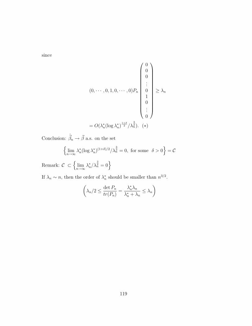
since
(0, · · · , 0, 1, 0, · · · , 0)Pn
000...010...0
≥ λn
= O(λ∗n(log λ∗n)1+δ2 /λ
32n ). (∗)
Conclusion: ~βn → ~β a.s. on the setlimn→∞
λ∗n(log λ∗n)(1+δ)/2/λ
32n = 0, for some δ > 0
= C
Remark: C ⊂
limn→∞
λ∗n/λ32n = 0
If λn ∼ n, then the order of λ∗n should be smaller than n3/2.(
λn/2 ≤detPntr(Pn)
=λ∗nλnλ∗n + λn
≤ λn
)
119

Example 1 : yi = β1 + β2i+ εi
i = 1, 2, 3, · · · , n.
~xi =
(1i
)
Pn =n∑i=1
~xi~x′i =
n
n∑i=1
i
n∑i=1
i
n∑i=1
i2
implies tr(Pn) = n+
n∑i=1
i2 ∼ n3.
det(Pn) = n
n∑i=1
i2 −
(n∑i=1
i
)2
∼ n n3/3−(n2
2
)2
=n4
3− n4
4=n4
12.
implies λ∗n ∼ n3
λn ∼ n
implies (∗) is not satisfy.Example 2 : AR (2)zn = β1zn−1 + β2zn−2 + εnCharacteristic polynomialP (λ) = λ2 − β1λ− β2
The roots of P (λ) determine the behavior of zn , assume that
P (λ) = (λ− ρ1)(λ− ρ2)
= λ2 − (ρ1 + ρ2)λ+ ρ1ρ2
β1 = ρ1 + ρ2, β2 = −ρ1ρ2
yn = zn, ~xn =
(zn−1
zn−2
)Depcomposition:(
vnwn
)=
(1 −ρ1
1 −ρ2
)(znzn−1
)=
(zn − ρ1zn−1
zn − ρ2zn−1
)120
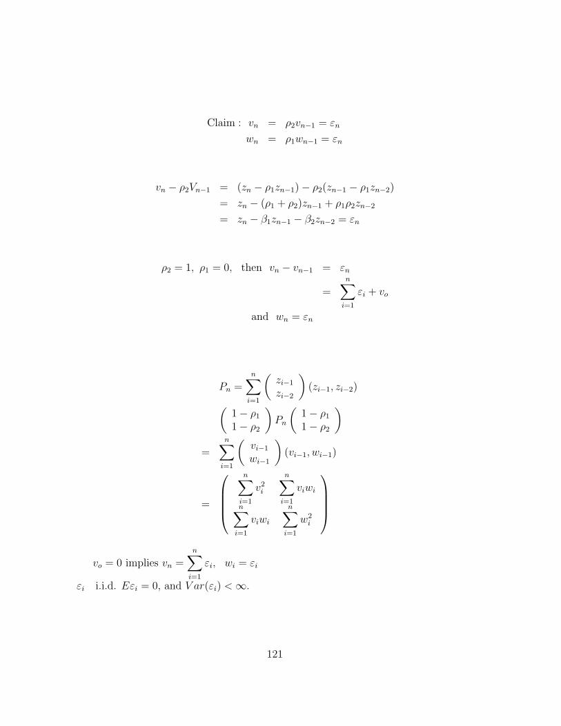
Claim : vn = ρ2vn−1 = εn
wn = ρ1wn−1 = εn
vn − ρ2Vn−1 = (zn − ρ1zn−1)− ρ2(zn−1 − ρ1zn−2)
= zn − (ρ1 + ρ2)zn−1 + ρ1ρ2zn−2
= zn − β1zn−1 − β2zn−2 = εn
ρ2 = 1, ρ1 = 0, then vn − vn−1 = εn
=n∑i=1
εi + vo
and wn = εn
Pn =n∑i=1
(zi−1
zi−2
)(zi−1, zi−2)(
1− ρ1
1− ρ2
)Pn
(1− ρ1
1− ρ2
)=
n∑i=1
(vi−1
wi−1
)(vi−1, wi−1)
=
n∑i=1
v2i
n∑i=1
viwi
n∑i=1
viwi
n∑i=1
w2i
vo = 0 implies vn =n∑i=1
εi, wi = εi
εi i.i.d. Eεi = 0, and V ar(εi) <∞.
121

tr(Pn) on order
(n∑i=1
v2i
)+
(n∑i=1
ε2i
)
det(Pn) =
(n∑i=1
v2i
)(n∑i=1
ε2i
)−
(n∑i=1
viεi
)2
=
(n∑i=1
v2i
)(n∑i=1
ε2i
)−
(n∑i=1
ε2i +
n∑i=1
vi−1εi
)2
Because vi = vi−1 + εi.
limn→∞
supn∑i=1
v2i /n(2n log log n) <∞ a.s. (Donsker Theorem)
limn→∞
inf(log log n)n∑i=1
v2i
n2> 0 a.s.
implies tr(Pn) ∼n∑i=1
v2i
Becausen∑i=1
vi−1εi = 0
( n∑i=1
v2i−1
)(log
[n∑i=1
v2i−1
]) 1+δ2
.
det(Pn) = −O
n2 +
(n∑i=1
v2i−1
)(log
n∑i=1
v2i−1
) 1+δ2
+
(n∑i=1
v2i
)(n∑i=1
ε2i
).
=
(n∑i=1
v2i
)(n∑i=1
ε2i
)1−O
n2 +
(n∑i=1
v2i−1
)(log
n∑i=1
v2i−1
)1+δ
(n∑i=1
v2i=1
)(n∑i=1
ε2i
)
122

n2
/(n∑i=1
v2i−1
)(n∑i=1
ε2i
)∼ n(
n∑i=1
v2i−1
)
= O(n/(n2/ log log n)) = O
(log log n
n
)[log
(n∑i=1
v2i−1
)]1+δ/ n∑i=1
ε2i = O
((log n)1+δ
n
)= o(1)
implies
tr(Pn) ∼n∑i=1
v2i
det(Pn) ∼
(n∑i=1
v2i
)· n
Not application I< 2 > Second ApproachEnergy function, ε-Liapounov′s function.dε(x(t))/dt < 0Roughly speaking, construct a constant function.
V : <P → <V (~x) > 0, if ~x 6= ~0
V (~0) = 0
inf|~x|>M
V (~x) > 0
If ~wn is a sequence of vectors in <ns.t.
V (~wn+1) ≤ V (~wn) and limn→∞
V (~ωn) = 0
then limn→
~wn = ~0.
123
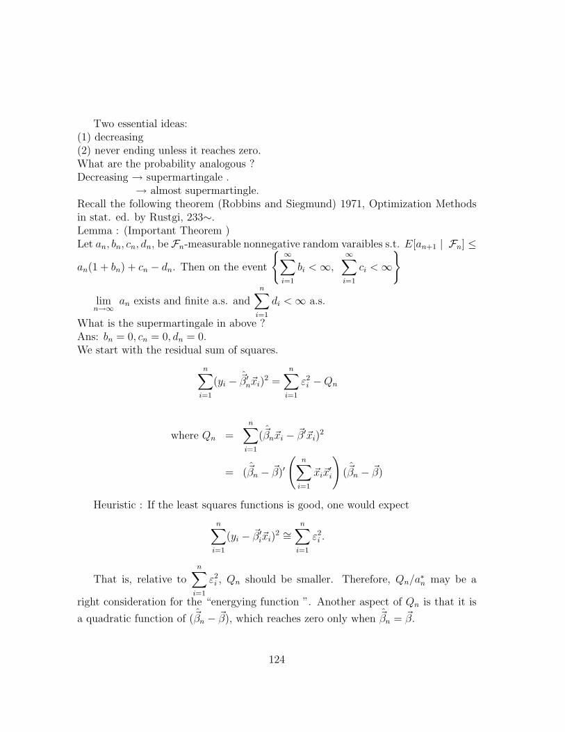
Two essential ideas:(1) decreasing(2) never ending unless it reaches zero.What are the probability analogous ?Decreasing → supermartingale .
→ almost supermartingle.Recall the following theorem (Robbins and Siegmund) 1971, Optimization Methodsin stat. ed. by Rustgi, 233∼.Lemma : (Important Theorem )Let an, bn, cn, dn, be Fn-measurable nonnegative random varaibles s.t. E[an+1 | Fn] ≤
an(1 + bn) + cn − dn. Then on the event
∞∑i=1
bi <∞,
∞∑i=1
ci <∞
limn→∞
an exists and finite a.s. andn∑i=1
di <∞ a.s.
What is the supermartingale in above ?Ans: bn = 0, cn = 0, dn = 0.We start with the residual sum of squares.
n∑i=1
(yi − ~β′n~xi)2 =
n∑i=1
ε2i −Qn
where Qn =n∑i=1
(~βn~xi − ~β′~xi)2
= (~βn − ~β)′
(n∑i=1
~xi~x′i
)(~βn − ~β)
Heuristic : If the least squares functions is good, one would expect
n∑i=1
(yi − ~β′i~xi)2 ∼=
n∑i=1
ε2i .
That is, relative ton∑i=1
ε2i , Qn should be smaller. Therefore, Qn/a
∗n may be a
right consideration for the “energying function ”. Another aspect of Qn is that it is
a quadratic function of (~βn − ~β), which reaches zero only when ~βn = ~β.
124

How to choose a∗n ?
Qn ≥‖ ~βn − ~β ‖2 ·λnor Qn/λn ≥‖ ~βn − ~β ‖, choose : a∗n = λn.
Theorem : In the stochastic regression model.
yn = ~β′~xi + εi
if supnE[ε2
n | Fn−1] <∞ a.s.
then on the event∞∑n=p
~x′n
(n∑i=1
~xi~x′i
)−1
~xn/λn <∞, limn→∞
λn = ∞
proof : an = Qn/λn, bn = 0.
Qn =
(n∑i=1
~xiεi
)′( n∑i=1
~xi~x′i
)−1( n∑i=1
~xiεi
)
E[an | Fn−1] =
(n−1∑i=1
~xiεi
)′
Vn
(n−1∑i=1
~xiεi
)/λn
+2E[~x′nεnVn
(n−1∑i=1
~xiεi
)| Fn−1]/λn
+E(~x′nVnεn | Fn−1)/λn.
=
(n∑i=1
~xiεi
)′
Vn
(n∑i=1
~xiεi
)/λn
+~x′nVn~xnE[ε2n | Fn−1]/λn
≤
(n−1∑i=1
~xiεi
)′
Vn−1
(n−1∑i=1
~xiεi
)/λn + cn−1
= Qn−1/λn + cn−1
= Qn−1/λn−1 −Qn−1
(1
λn−1
− 1
λn
)+ cn−1
= an−1 − an−1(1− λn−1/λn) + cn−1
125

By the almost supermartingale theorem.
limn→∞
an <∞ and
(∑an−1
(λn − λn−1
λn
))<∞
a.s. on ∑
cn−1 <∞ =
∑ ~x′nVn~xnλn
E[ε2n | Fn−1] <∞
⊃
∑ ~x′nVn~xnλn
<∞
If limn→∞
an = a > 0
Then ∃N s.t. an ≥ a/2, ∀ n > N
So∞∑i=1
ai−1λi − λi−1
λi≥ a
2
(∞∑i=N
λi − λi−1
λi
)
≥ a
2
∞∑i=N
∫ λi
λi−1
dx
x· λn/λn−1
≥ a
2
(infn≥N
λn/λn−1
)∫ ∞
λn−1
1
xdx = ∞
Note 1: If λn−1/λn has limit point λ < 1 then there exists
nj 3 limj→∞
λnj−1/λnj = λ, lim
j→∞
λnj − λnj−1
λnj= 1− λ.
This contradicts.
Note 2 : If∑i
λi − λi−1
λi<∞
Then λn−λn−1
λn→ 0
λn−1/λn → 1.Therefore, on the event ∑ ~xnVn~xn
λ<∞, λn →∞
,
an → 0 a.s.
since an ≥‖ ~βn − ~β ‖2
~βn → ~β a.s. on the same event.
126
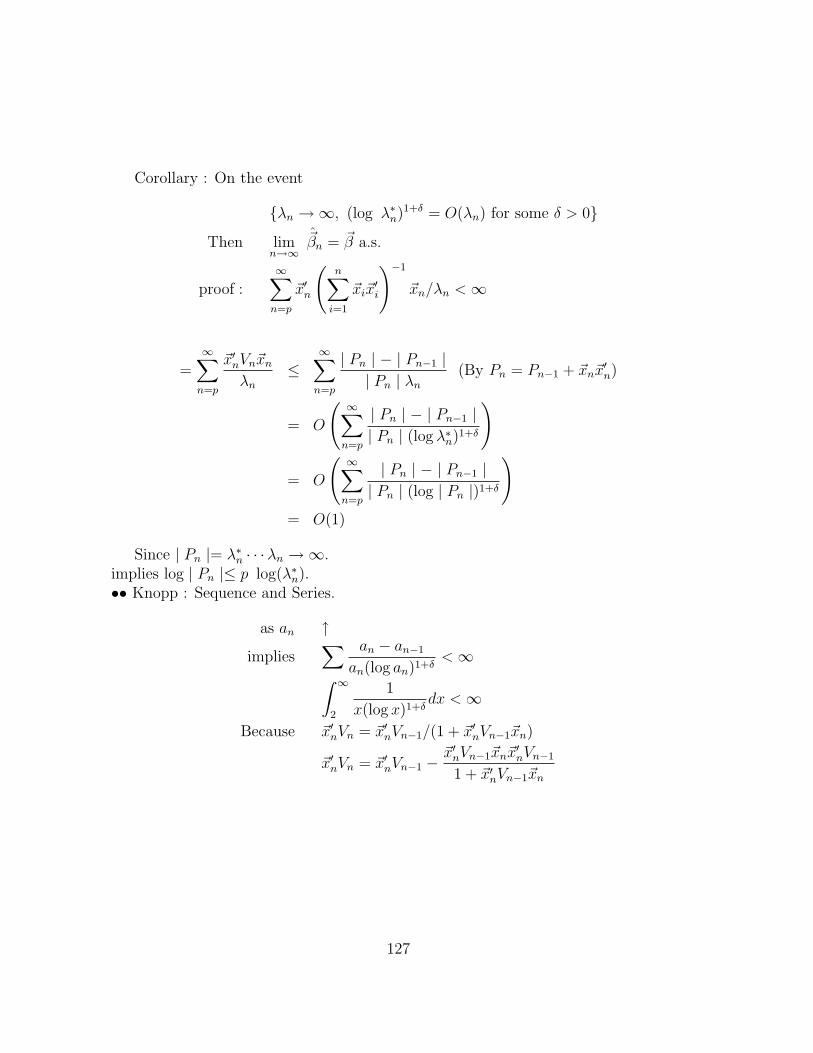
Corollary : On the event
λn →∞, (log λ∗n)1+δ = O(λn) for some δ > 0
Then limn→∞
~βn = ~β a.s.
proof :∞∑n=p
~x′n
(n∑i=1
~xi~x′i
)−1
~xn/λn <∞
=∞∑n=p
~x′nVn~xnλn
≤∞∑n=p
| Pn | − | Pn−1 || Pn | λn
(By Pn = Pn−1 + ~xn~x′n)
= O
(∞∑n=p
| Pn | − | Pn−1 || Pn | (log λ∗n)1+δ
)
= O
(∞∑n=p
| Pn | − | Pn−1 || Pn | (log | Pn |)1+δ
)= O(1)
Since | Pn |= λ∗n · · ·λn →∞.implies log | Pn |≤ p log(λ∗n).•• Knopp : Sequence and Series.
as an ↑
implies∑ an − an−1
an(log an)1+δ<∞∫ ∞
2
1
x(log x)1+δdx <∞
Because ~x′nVn = ~x′nVn−1/(1 + ~x′nVn−1~xn)
~x′nVn = ~x′nVn−1 −~x′nVn−1~xn~x
′nVn−1
1 + ~x′nVn−1~xn
127
< 3 > Third Approach:
Qk =
(k∑i=1
~xiεi
)′
Vk
(k∑i=1
~xiεi
)
=
(k−1∑i=1
~xiεi
)′
Vk
(k−1∑i=1
~xiεi
)
+~x′kVk~xkε2k + 2(~x′k~xk
k−1∑i=1
~xiεi)εk
= Qk−1 − (~x′kVk−1
k−1∑i=1
~xiεi)2/(1 + ~x′kVk−1~xk)
+~x′kVk~xkε2k + 2(~x′kVk
k−1∑i=1
~xiεi)εk.
Qn −QN =n∑
j=N+1
(Qj −Qj−1)
= −n∑
k=N+1
(~x′kVk−1
k−1∑i=1
(~xiεi)2
)2/(1 + ~x′kVk−1~xk)
+n∑
k=N+1
~x′kVk~xkε2k + 2
n∑k=N+1
(~x′kVk
k−1∑i=1
~xiεi
)εk
128
implies Qn −QN +n∑
k=N+1
(~x′kVk−1
k−1∑i=1
~xiεi
)2
/(1 + ~x′kVk−1~xk)
(1) =n∑
k=N+1
~x′kVk~xkε2k + 2
n∑k=N+1
(~x′kVk−1
k−1∑k=1
~xiεi
)1 + ~x′kVk−1~xk
εk
(2) =n∑
k=N+1
(~x′kVk−1
k−1∑i=1
~xiεi
)2
/(1 + ~x′kVk−1~xk)
=n∑
i=N+1
(~x′kVk−1
k−1∑i=1
~xiεi
)1 + ~x′kVk−1~xk
εk
(1) finite if and only if (2) finite.Theorem: If sup
nE[ε2
n | Fn−1] <∞ a.s.
Then
−QN +Qn +n∑
k=N+1
(~x′kVk−1
k−1∑i=1
~xiεi
)2
1 + ~x′kVk−1~xk
∼n∑
k=N+1
~x′kVk~xkε2k a.s.
on the set where one of it approaches ∞.proof: Let
Uk =
~x′kVk−1
k−1∑i=1
~xiεi
1 + ~x′kVk−1~xk
Then Uk is Fk−1-measurable.
129
Therefore
n∑k=N+1
Ukεk =
O
(n∑
k=N+1
U2k
)on
[n∑
k=N+1
U2k <∞
]
o
(n∑
k=N+1
U2k
)on
[∞∑
k=N+1
U2k = ∞
]
Butn∑
N+1
U2k ≤
n∑N+1
U2k (1 + ~x′kVk−1~xk)
=n∑
N+1
(~x′kVk−1
k−1∑i=1
~xiεi
)2
/(1 + ~x′kVk−1~xk)
Special case ~xi = 1, Pn = n.
(n∑i=1
εi
)2/n+
n∑k=N+1
k−1∑i=1
εi
k − 1
2
/(1 +
1
k − 1
)
∼n∑
k=N+1
ε2k
kn∑
k=N+1
k−1∑1
εi
k − 1
2/(
1 +1
k − 1
)=
n∑k=N+1
(k − 1
k
)(εk−1)
2
)
130
Because∑
(εk)2 ∼ (log n)σ2.
Qn +n∑
k=N+1
(~x′kVk+1
k−1∑i=1
~xiεi)2/(1 + ~x′kVk−1~xk)
∼n∑
k=N+1
~x′kVk~xkε2k, if one of it →∞, where
Qn = (~βn − ~β)
(n∑i=1
~xi~x′i
)(~βn − ~β)
=
(n∑i=1
~xiεi
)′
Vn
(n∑i=1
~xiεi
).
Lemma : Assume that εk,Fk is a martingale difference sequence and Vk is Fk−1-measurable all k.(i) Assume that sup
nE[ε2
n | Fn−1] <∞ a.s.
Then∞∑k=1
| uk | ε2k <∞ a.s. on
∞∑k=1
| uk |<∞
and∞∑k=1
| uk | ε2k = o
( n∑k=1
| uk |
)(log
n∑k=1
| uk |
)1+δ .
on the set
∞∑k=1
| uk |= ∞
, for all δ > 0.
(ii) Assume that supnE[| εn |α| Fn−1] <∞, for some α > 2. Then
n∑k=1
| uk | ε2k −
n∑k=1
| uk | E[ε2k | Fk−1]
= o
(n∑k=1
| uk |
)a.s. on
∞∑k=1
| uk |= ∞, supn| un |<∞
.
131

Therefore, if limk→∞
E[ε2k | Fk−1] = σ2 a.s.
Then limn→∞
n∑k=1
| uk | ε2k/
n∑k=1
| uk |= σ2 a.s.
on
∞∑k=1
| uk |= ∞, supn| un |<∞
Note:Basic idea is to ask : zi ≥ 0, the relation of
n∑i=1
zi andn∑i=1
E[zi | Fi−1]
Becausen∑k=1
E(| uk | ε2k | Fk−1) =
n∑k=1
| uk | E(ε2k | Fk−1)
(Freedman. D. (1973). Ann. Prob. 1, 910∼925.).proof: (i) Take an large enough so that
∞∑k=1
P [| uk |> ak] <∞
Let u∗k = ukI[|uk|≤ak]
Then Puk = u∗k eventually =1.If we can show our results for u∗k then the results also hold for uk.Therefore, we can assume that each uk is a bounded random variables.∀ M > 0, define
vk = ukI[E(ε2k|Fk−1)≤M ]Ik∑i=1
| ui |≤M
then vk is Fk−1-measurable.
Then E
(∞∑i=1
| vi | ε2i
)=
(∞∑i=1
E(| vi | ε2i | Fi−1)
)
= E
(∞∑i=1
| vi | E[ε2i | Fi−1]
)
132
≤ E
∞∑i=1
| ui | Ii∑
j=1
| uj |≤M
·M
≤M2 <∞
So∞∑i=1
| vi | ε2i <∞ a.s.
Observe that vk = uk, ∀ k on
supnE[ε2
n | Fn−1] ≤M,∞∑n=1
| un |≤M
= ΩM .
So∞∑i=1
| ui | ε2i <∞ a.s. on ΩM , ∀ M .
But∞⋃
M=1
ΩM =
supnE[ε2
n | Fn−1] <∞,∞∑n=1
| un |<∞
.
=
∞∑n=1
| un |<∞
The proof is first part.
Let sn =n∑i=1
| ui |
considern∑k=1
| uk | ε2k
sk(log sk)1+δ
Since∞∑n=1
| un |sn(log sn)1+δ
<∞ a.s.
≤∞∑n=1
∫ sn
sn−1
dx
x(log x)1+δ
implies∞∑k=1
| uk |sk(log sk)1+δ
ε2k <∞ a.s.
133

By Kronecker′s Lemma, on
sn =
n∑i=1
| ui |→ ∞
limn→∞
n∑k=1
| uk | ε2k
sn(log sn)1+δ= 0 a.s.
(ii) (Chow (1965), local convergence theorem).For a martingale difference sequence δk, Fkn∑k=1
εk converges a.s. on∞∑k=1
E(| δk |r| Fk−1) <∞
.
where 1 ≤ r ≤ 2.Set δk = u2
k[ε2k − E(ε2
k | Fk−1)]Then δk,Fk is a martingale difference sequence without loss of generality,
we can assume that 2 < α ≤ 4. If α ≥ 4, then E14 (ε4
i | Fi−1) ≤ E1α (| εi |α| Fi−1).
Set r = α/2.Let tn =
∑ni=1 | ui |2r .
E[| δk |r| Fk−1]
=| uk |2r E| ε2k − E[ε2
k | Fk−1] |r| Fk−1≤ | uk |2r E[max
k(| ε2
k |, E[ε2k | Fk−1]
r | Fk−1
≤ | uk |2r E| εk |2r +Er[ε2k | Fk−1] | Fk−1
= | uk |2r E[| εk |2r| Fk−1] + Er[ε2k | Fk−1]
≤ 2 | uk |2r E[| εk |2r| Fk−1]
Son∑k=1
E(| δk/tk |r| Fk−1)
≤ 2
(n∑k=1
| uk |2r
trk
)supnE[| εn |α| Fn−1] <∞ a.s.
Son∑k=1
δk = o(tn) a.s. on tn →∞
Butn∑k=1
δk converges a.s. on
∞∑i=1
| ui |2r= limn→∞
tn <∞
.
134

by Chow′s Theorem onn∑i=1
δi.
Observe that on supn | un |<∞.
tn ≤
(n∑i=1
| ui |
)(supn| un |2r−1
)Combining all those results
n∑i=1
δi = o
(n∑i=1
| ui |
)a.s. on
∞∑i=1
| ui |= ∞, supn| un |<∞
.
It is not difficult to see that
n∑k=1
| uk | ε2k = O
(n∑k=1
| uk |
)a.s. on
supn| un |<∞
This is because
(a) On
n∑i=1
| ui | < ∞, supn| un |<∞
,
n∑k=1
| uk | ε2k = O(1) = O
(n∑k=1
| uk |
)(by (i))
(b) On
n∑k=1
| uk | = ∞, supn| un |<∞ ,
n∑k=1
| uk | ε2k =
n∑k=1
| uk | E(ε2k | Fk−1) + o
(n∑k=1
| uk |
)
≤
(n∑i=1
| ui |
)supnE(ε2
n | Fn−1) + o
(n∑k=1
| uk |
)
=
(n∑i=1
| ui |
)(supnE(ε2
n | Fn−1) + o(1)
)
= O
(n∑i=1
| ui |
).
135
Now, if limn→∞
E[ε2n | Fn−1] = σ2.
Thenn∑k=1
| uk | E[ε2k | Fk−1]/
n∑k=1
| uk |→ σ2 a.s. on
∞∑k=1
| uk |= ∞
.
By an ≥ 0, bn ≥ 0, bn → b,
n∑i=1
ai →∞
Thenn∑i=1
aibi/n∑i=1
ai → b.
Son∑k=1
| uk | ε2k/
n∑k=1
| uk |
=
n∑k=1
| uk | E[ε2k | Fk−1]
n∑k=1
| uk |+ o(1)
→ σ2, a.s. on
supn| un |<∞,
∞∑k=1
| uk |= ∞
.
Lemma 2: Let wn be a p× 1 vectors and
An =n∑i=1
~wi ~w′i. Assume that AN is nonsingular for some N . Let λ∗n and | An | denote
the maximum evgenvalue and determinant of An.
Then (i) λ∗n ↑ .
(ii) limn→∞
λ∗n <∞ implies∞∑i=N
~w′iAi ~wi <∞.
(iii) limn→∞
λ∗n = ∞, impliesn∑
i=N
~w′iA
−1i ~wi = O(log λ∗n).
(iv) limn→∞
λ∗n = ∞, ~w′iA
−1i ~wi → 0, implies
n∑i=N
~w′iA
−1i ~wi ∼ log | An | .
136
proof : (i) trivial.
(ii) ~w′n A
−1n ~wn =
| An | − | An−1 || An |
(λ∗n)p ≥| An | and | An |≥ λ∗nλ
p−1n
Where λn is the minimum eigenvalue of An.
If λ∗n <∞, then limn→∞
| An |<∞.
So∞∑i=N
~w′iA
−1i ~wi =
∞∑i=N
| Ai | − | Ai−1 || Ai |
≤
∞∑i=N
(| Ai | − | Ai−1 |)
| Ai |=
limn→∞
| An | − | AN−1 |
| AN |<∞.
(iii) Note thatn∑
i=N
~w′iA
−1i ~wi =
n∑i=N
| Ai | − | Ai−1 || Ai |
≤n∑
i=N+1
∫ |Ai|
|Ai−1|
1
xdx+ 1
= 1 + log | An | − log | AN |= O(log | An |) = O(log λ∗).
(iv) Note that λ∗n →∞, | An |→ ∞.
Now| An | − | An−1 |
| An |→ 0 implies
n∑i=N
| Ai | − | Ai−1 || Ai |
∼ log | An |
137
Corollaryl : (1) If supnE[ε2
n | Fn−1] <∞ a.s.
Thenn∑
k=N+1
~x′kVkε2k
= O((log λ∗n)1+δ) a.s.
(2) If supnE[| εn |2+δ| Fn−1] <∞, for some δ > 0.
Then
(i)n∑
k=N+1
~x′kVk~xkε2k = O(log λ∗n) a.s.
(ii) limn→∞
E[ε2n | Fn−1] = σ2. Then
n∑k=N+1
~x′kVk~xkε2k ∼ log
(det
(n∑k=1
~xk~x′k
))on
limn→∞
~x′nVn~xn = 0, λ∗n →∞.
proof : 0 ≤ uk = ~x′kVk~xk =| Pk | − | Pk−1 |
| Pk |≤ 1
(1) If limn→∞
λ∗n <∞ then∑∞
k=1 uk <∞ (lemma 2 - (ii)).
Therefore∞∑k=1
ukε2k <∞ (by lemma 1-(i)).
Son∑k=1
ukε2k = O((log λ∗n)
1+δ) on (λ∗n →∞)
If λ∗n →∞,n∑i=1
ui = O(log λ∗n).
andn∑i=1
uiε2i = O(
(n∑i=1
ui
)[log
(n∑i=1
ui
)]1+δ)
= O(log λ∗n(log log λ∗n)1+δ)
= O((log λ∗n)1+δ).
138

(2) Note that 0 ≤ ui ≤ 1.
un → 0 on Ωo, Ωo = limn→∞~x′nVn~xn = 0, λ∗n →∞ .
n∑i=1
ui →∞ on Ωo
By lemma 1 - (ii),n∑i=1
uiε2i /
n∑i=1
ui → σ2 a.s.
onn∑i=1
uiε2i ∼ (log | Pn |)σ2
Remark:
1o Rn = Qn +n∑
k=N+1
(~x′kVk
k−1∑i=1
~xiεi
)2
/(1 + ~x′kVk−1~xk)
∼n∑
k=N+1
~x′kVk~xkε2k if one of it →∞.
2o (i) Assume that supnE[ε2
n | Fn−1] <∞ a.s.
Then Rn = O((log λ∗n)1+δ) a.s. for δ > 0
(ii) If supnE[| εn |2+δ| Fn−1] <∞ a.s. for some α > 2,
Then Rn = O(log λ∗n)
3o If supnE[| εn |α| Fn−1] <∞ a.s. and lim
n→∞E[ε2
n | Fn−1] <∞ a.s.
then on ~x′nVn~xn → 0, λ∗n →∞
Rn ∼ [log det
(n∑i=1
~xi~x′i
)]σ2 a.s.
Corollary 1 : (i) If supnE[ε2
n | Fn−1] <∞ a.s.
Then Qn =‖
(n∑i=1
~xi~x′i
)−1/2 n∑i=1
~xiεi ‖2 (∗)
= O((log λ∗n)1+δ) a.s. (∗∗)
139

and ‖ ~bn − ~β ‖2= O((log λ∗n)1+δ/λn) a.s., for all δ > 0.
(ii) If supnE[| εn |α| Fn−1] <∞ a.s. for some α > 2,
then (∗) and (∗∗) holds with δ = 0
proof : Qn ≤ Rn (implies (∗) follow from Remark− 2o)
Qn =
(n∑i=1
~xiεi
)′( n∑i=1
~xi~x′i
)−1( n∑i=1
~xiεi
)
= (~bn − ~β)′
(n∑i=1
~xi~x′i
)(~bn − ~β)
≥ λn(~bn − ~β)′(~bn − ~β)
= λn ‖ ~bn − ~β ‖2 .
So (∗∗) follow from (∗).Corroblary 2: (Adaptive prediction)If lim
n→∞E[ε2
n | Fn−1] = σ2 a.s. and
supnE[| εn |α| Fn−1] <∞ for some α > 2
then on the set
~x′nVn~xn → 0, λ∗n →∞, we have that
Qn +n∑
k=N+1
(~bk−1 − ~β)′~xk2.
∼ σ2 log
[det
(n∑i=1
~xi~x′i
)]a.s.
Therefore, if Qn = 0(log λ∗n), then
n∑k=N+1
(yk −~b′
k−1~xk − εk)2 ∼ σ2 log[det
(n∑i=1
~xi~x′i
)] a.s.
140

proof: By Remark- 3o ,
Qn +n∑
k=N+1
(~x′kVk
k−1∑i=1
~xiεi
)2
/(1 + ~x′kVk−1~xk)
Qn +n∑
k=N+1
~x′k(~bk−1 − ~β)2/(1 + ~x′kVk−1~xk)
∼ σ2 log[det
(n∑i=1
~xi~x′i
)] a.s.
n∑k=N+1
[~x′k(~bk−1 − ~β)]2/(1 + ~xkVk−1~xk)
∼n∑
k=N+1
[~x′k(~bk−1 − ~β)]2 if it →∞ and ~x′kVk−1~xk → 0,
since 1 + ~x′kVk−1~xk =1
1− ~x′kVk~xk→ 1.
andn∑i=1
aibi ∼n∑i=1
ai (aibi > 0)
if bi → 1 andn∑i=1
ai →∞
(Because yk = ~β′~xk + εk)
Predict:At stage n, we already above y1, ~x1, · · · , yn, ~xn since we can not forsee the
future, we have to use observed data to predict yn+1.i.e. The predictor yn+1 is Fn-measurable.
If we are only interested in a single period prediction, we may use (yn+1− yn+1)2 as
a measure of performance. In the adaptive prediction case, it may be more appropriateto use the accumulated prectiction errors
Ln =n∑k=1
(yk+1 − yk+1)2
141

In the stochastic regression model,
Ln =n∑k=1
(~β′~xk+1 − yk+1)2
+2n∑k=1
(~β′~xk+1 − yk+1)εk+1 +n∑k=1
ε2k+1
By Chow′s local convergence Theorem,
Ln ∼n∑k=1
(~β′~xk+1 − yk+1)2 +
n+1∑k=1
εk a.s. if any side →∞.
Therefore, to compare difference predictors, it is sufficient to compare
n∑k=1
(~β′~xk+1 − yk+1)2 = Cn
The least square predictor yk+1 = ~b′k~xk+1.
Note :n∑
i=P+1
(yi −~b′i−1~xi)2(1− ~x′iVi~xi)
=n∑i=1
ε2i (n)−
n∑i=1
ε2i (p), where εi(n) = yi −~b′n~xi
Example : AR(1)
xk = ρxk−1 + εk, εk ∼ i.i.d..
E[εi] = 0, V ar(εi) = σ2, E | εi |3<∞
(i) | ρ |< 1,n∑i=1
x2i /n→ σ2/(1− ρ2) a.s.
(ii) | ρ |= 1,n∑i=1
x2i = O(n2 log log n)
142
limn→∞
inf
(log log n)
(n∑1
x2i
)n2
> 0 a.s.
λ∗n = O(n3) a.s., | ρ |≤ 1.
limn→∞
inf λn/n > 0
ρn − ρ = 0
(log n
n
)1/2
(By Corollary1.)
x2n/
n∑i=1
x2i → 0
(i) | ρ |< 1, x2n/
n∑i=1
x2i =
n∑i=1
x2i /n−
n−1∑i=1
x2i /n
n∑i=1
x2i /n
→ 0
1/(1− ρ2)= 0
(ii) | ρ |= 1,
x2n/
n∑i=1
x2i = O
( n∑i=1
εi
)2
/(log log n/n2)−1
= O
(log log n
n2(√
2n log log n)2
)= O
((log log n)2
n
)= o(1)
143

Qn =
(n∑i=1
xiεi
)2
/n∑i=1
x2i
=
1(n∑i=1
x2i
)( n∑
i=1
x2i
)1/2(log
n∑i=1
x2i
)1/32
=
(log
n∑i=1
x2i
)2/3
= (log n)2/3 = 0(log λ∗n)
By Corolary 2,
n∑i=2
(ρn − ρ)x2i+1 ∼ σ2 log
(n+1∑i=1
x2i
)a.s.
∼σ2 log n, a.s. if | ρ |< 1.2σ2 log n, a.s. if | ρ |= 1.
log[n2 log log n] = 2 log n+ log(log log n)
log[n2/ log log n] = 2 log n− log(log log n).
To find the eigenvalue (maximum and minimum)
inf‖~x‖=1
~x′Bn~x nonnegative positive
1o limn→∞
inf
inf‖~x‖=1
~x′Bn~x
6= inf
‖~x‖=1
limn→∞
~x′Bn~x
(The place of difficulity)
2o Lemma : Assume that Fn be a sequence of ↑ σ -fields and ~yn = ~xn + ~εn,when
~xn is Fn−`-measurable, ~εn =∑j=1
~εn(j) and E~εn(j) | Fn−j−1 = 0.
144
supnE[‖~εn(j)‖α | Fn−j−1] < ∞ a.s. for some α > 2. Also assume that λn =
λ
(n∑i=1
~xi~x′i +
n∑i=1
~εi~ε′i
)→∞ a.s. and log λ∗
(n∑i=1
~xi~x′i
)= 0 (λn) a.s.
Then limn→∞
λ
(n∑i=1
~yi~y′i
)/λn = 1 a.s.
proof : Let Rn =n∑i=1
~xi~x′i and Gn =
n∑i=1
~εi~ε′i
Thenn∑i=1
~yi~y′i = Rn +
n∑i=1
~xi~ε′i +
n∑i=1
~εi~xi +Gn
We can assume that Rn is nonsingular.
Otherwise, add ~yo =
10...0
= ~xo
~y−1 = ~x−1 =
010...0
...
~y1−P = ~x1−P =
00...01
εo = ε−1 = · · · = ε−P+1 = 0
‖R− 12
n
n∑1
~xi~ε′i(j)‖2 = O(log(λ∗n)), (By Corollary 1.)
= o(λn)
145

Therefore ‖R− 12
n
n∑1
~xi~εi‖2 = O(log λ∗n)
Given any unit vector ~u ,
~u′
(n∑1
~xi~εi
)~u
= ~u′R12nR
− 12
n
(n∑1
~xi~ε′i
)~u
≤ ‖~u′R12n‖‖R
− 12
n
(n∑1
~xi~ε′i
)‖
= ‖~u′R12n‖O((log λ∗n)
12 )
= (~u′Rn~u)12O((log λ∗)
12 )
≤ (~u′(Rn +Gn)~u)12O(log
12 λ∗n)
≤ (~u′(Rn +Gn)~u/λ12n ) O(log
12 λ∗n)
(Because 1 ≤ ~u′(Rn +Gn)~u)/λn)
= ~u′(Rn +Gn)~u O((log λ∗n/λn)12 )
= (~u′(Rn +Gn)~u)o(1)
So ~u′
(n∑1
~yi~y′i
)~u = ~u′(Rn +Gn)~u(1 + o(1))
Since o(1) does not depend on ~u, we complete this proof.Example :AR(p).
yi = β1yi−1 + · · ·+ βpyi−p + εi
ψ(z) = zp − β1zp−1 · · · − βp.
All the roots of ψ have magnitudes less than or equal to 1.
Let ~yn =
ypyp+1
...yn−p+1
146

Then L.S.E.
~bn =
(n∑i=1
~yi−1~y′i−1
)−1( n∑i=1
yi−1εi
)+ ~β
Assume that εi are i.i.d.
E[εi] = 0 and E[| εi |2+δ] <∞, Eε2i = σ2 > 0.
Let B =
[β1 · · · βpIp−1 O
]
~yn =
ynyn−1
...yn−p+1
=
β1 β2 · · · βp1 0 · · · 00 1 · · · 0...
......
0 0 1 0
yn−1
yn−2...
yn−p
+
εn00...0
implies ~yn = B ~yn−1 + ~e εn, where e =
10...00
~yn = Bnyo +Bn−1~eεn + · · ·+Bo~eεn
B can be written as
B = C−1DC, where D = diag [D1, · · · , Dq]
Dj =
λj 1 0 · · · 00 λj 1 · · · 0...
.... . .
...0 0 · · · λj
is an mj ×mj matrix, mj is the multiplicity of λj.
147
,
q∑1
mj = p, λj are roots of ψ and C is a nonsingular matrix.
Dkj =
λkj
(k1
)λk−1j
(k2
)λk−2j · · ·
(k
mj−1
)λk−mj+1
0 λkj 0 · · · 0
0 0. . .
......
......
. . .
0 0 0 · · · λkj
Bn = C−1DnC
= C−1diag[Dn1 , · · · , Dn
q ]C
‖Bn‖ ≤ ‖C−1‖‖C‖ max‖Dn1‖, · · · , ‖Dn
q ‖
≤ k np (By
(n
p
)=
n!
p!(n− p)!∼ np)
‖~yn‖ ≤ ‖Bn‖‖~yo‖+ · · ·+ ‖Bo~e‖ | εn |≤ k np‖~yo‖+ | ε1 | + · · ·+ | εn |= O(np+1)
λmax
(n∑i=1
~yi−1~y′i−1
)
≤ ‖n∑i=1
~yi−1~y′i−1‖
≤n∑i=1
‖~yi−1~y′i−1‖ ≤
n∑i=1
‖~yi−1‖2
= O
(n∑i=1
ip+1
)a.s.
= O(np+2) a.s.
148

implies λmax = O(np+2)
~yn = B2~yn−2 +B~eεn−1 + ~eεn
= Bp~yn−p +Bp−1~eεn−p+1 + · · ·+ ~eεn
= ~xn + ~εn, where
~xn = Bp~yn−p, ~εn = Bp−1~e εn−p+1 + · · ·+ ~e εn
` = p.
Claim : limn→∞
1
n
n∑i=1
~εi~ε′i = σ2
p−1∑j=0
Bj~e ~e′ (B′)j ≡ Γ, a.s.
where Γ is positive definite.
Therefore, λmin
(n∑i=1
~εi~ε′i
)/n→ λmin(Γ) > 0 a.s.
~εi ~ε′i =
p−1∑j=0
Bj~e~e′(B′)jε2i−j
+
p−1∑j 6=`
Bj~e ~e′(B′)`εi−jεi−`
Using the properties that
1/nn∑i=1
ε2i−j = σ2
1/nn∑i=1
εi−`εi−j = 0 a.s. ∀ ` 6= j.
(From Martingale form and by Chow′s theorem.)
We have limn→∞
1
n
n∑i=1
~εi~ε′i = Γ. a.s.
149

Observe that
Γ = (~e, B~e, · · · , Bp−1~e)
~e′
~e′B′
...~e′(B′)p−1
To show Γ is nonsingular, it is sufficient to show (~e,B~e, · · · , Bp−1~e) is nonsingular.
(~e,B~e, · · · , Bp−1~e) =
1 β1 ∗ ∗ · · · ∗0 1 β1 ∗ · · · ∗0 0 1...
......
0 0 0 · · · · · · 1
is nonsingular.
~xn = Bp~yn−p
λ∗
(n∑i=p
~xi~x′i
)≤ ‖Bp‖2
n∑i=p
~yi−p~y′i−p‖
= O(np+2) a.s.
But λn ≥ λ∗
(n∑i=1
~εi~ε′i
)∼ nλ∗(Γ)
So log λ∗
(n∑i=1
~xi~x′i
)= O(log n) = o(λn) a.s.
By previous theorem,
limn→∞
λ∗
(n∑i=1
~yi−1~y′i−1
)λn
= 1 a.s.
Therefore, limn→∞
inf λ∗
(n∑i=1
~yi−1~y′i−1
)/n > 0 a.s.
150

So log λ∗
(n∑i=1
~yi−1~y′i−1
)
= o
(λ∗
(n∑i=1
~yi−1~y′i−1
))and
limn→∞
~bn = ~β a.s.
3. Limiting Distribution :
yn,i = β′nxn,i + εn,i, i = 1, 2, · · · , n
Assume that ∀ n,∃ ↑ σ-fields Fn,j; j = 0, 1, 2, · · · , ns.t. ∀ n εn,j,Fn,j is a martingale difference sequence and xn,j is Fn,j−1-measurable.Assume that:
(i) E[ε2n,j | Fn,j−1] = σ2 a.s. ∀ n, j.
(ii) sup1≤j≤n
E[| εn,j |α| Fn,j−1] = OD(1), α > 2.
(iii) ∃ nonsingular matrices An s.t.
An
(n∑i=1
~xi,n~x′i,n
)A′n
D→ Γ, where Γ is p.d.
(iv) sup1≤i≤n
‖An~xn,i‖D→ 0.
Then if ~bn =
(n∑i=1
~xn,i~x′n,i
)−1( n∑i=1
~xn,iyn,i
), we have
(A′n)−1(~bn − ~β)
D→ N(0, σ2Γ−1)
take i = 1, 2, · · · , kn
151

Note: If Xn,j,Fn,j, 1 ≤ j ≤ kn is a martingale difference sequence s.t.
(i)kn∑j=1
E[X2n,j | Fn,j−1]
D→ C, constant
(ii)kn∑j=1
E[X2n,jIX2
n,j>ε | Fn,j−1]D→ 0
Thenkn∑j=1
Xn,jD→ N(0, C)
proof: W.L.O.G, we can assume thatxni is bounded,∀ n, i.
since (A′n)−1(~bn − ~β)
=
(An
kn∑i=1
~xn,i~x′n,iA
′n
)(An
kn∑i=1
~xn,iεn,i
)It is sufficient to show that
An
kn∑i=1
~xn,iεn,iD→ N(~o, σ2Γ)
By Wald′s device, it is sufficient to show that
∀ ~t 6= ~0
~t′An
kn∑i=1
~xn,iεn,iD→ N(0, σ2~t′Γ~t)
Let un,i = ~t′An~xn,iεn,iThen un,i,Fn,i is martingale difference s.t.
kn∑i=1
E(u2n,i | Fn,i−1) =
kn∑i=1
(~t′An~xn,i)2E[ε2
n,i | Fn,i−1]
= σ2
kn∑i=1
~t′An~xn,i~x′n,iA
′n~t
= σ2~t′An
kn∑1
~xn,i~x′n,iA
′nt
D→ σ2~t′Γ~t = C, say.
152

andkn∑i=1
E[u2n,iIu2
n,i>ε | Fn,i−1
]≤
kn∑i=1
E[| un,i |α| Fn,i−1]
/εα−2
2
=1
εα−2
2
kn∑i=1
| ~t′An~xn,i |α E[| εn,i |α| Fn,i−1]
≤ ε−(α−22 ) sup
1≤i≤knE[| εn,i |2| Fn,i−1]
kn∑i=1
| ~t′An~xn,i |2
· sup1≤i≤kn
| ~t′An~xn,i |α−2 .
≤ ε−(α−22 ) sup
1≤i≤knE[| εn,i |α| Fn,i−1] · ~t′An
(n∑i=1
~xn,i~xn,i
)A′n~t
·‖~t‖ sup1≤i≤kn
‖An~xn,i‖D→ 0.
Example : yo = 0
yn = α+ βyn−1 + εn, where | β |< 1, εn i.i.d., E[εn] = 0,
V ar[εn] = σα, E[| εn |2] <∞, for some α > 2.
yn = α+ β[α+ βyn−2 + εn−1] + εn
= α+ βα+ β2yn−2 + βεn−1 + εn
= α+ βα+ β2α+ · · ·+ βn−1α+ βn−1εn−1 + · · ·+ εn
Since α+ βα + β2α+ · · ·+ βn−1α+ · · ·= α(1 + β + β2 + · · ·+ βn−1 + · · · )
= α1
1− β.
153
implies1
n
n∑i=1
y2i →
(α
1− β
)2
+σ2
(1− β)2
1
n
n∑i=1
yi →α
1− βa.s.
yn = (α, β)
(1
yn−1
)= ~β′~xn
1
n
n∑i=1
(1yi−1
)(1, yi−1)
=1
n
n
n∑i=1
yi−1
n∑i=1
yi−1
n∑i=1
y2i−1
→
(1 α/(1− β)
α/(1− β)(
α1−β
)2
+ σ2
(1−β)2
)≡ Γ.
take (√n)−1 = A
Now, kn = n
sup1≤i≤n
‖ 1√n
(1yi−1
)‖
≤ 1√n
+1√n
sup1≤i≤n
| yi−1 |
It is sufficient to show that
yn−1/√n→ 0 a.s.
y2n−1/n =
n−1∑i=1
y2i −
n−2∑i=1
y2i
n→ 0 a.s.
An
(kn∑1
~xn,i~x′n,i
)A′n → Γ a.s.
An/An−1 → 1 a.s.
implies sup1≤i≤kn
‖An~xn,i‖D→ 0.
154
![A FINITE ELEMENT METHOD FOR MARTINGALE …209].pdf · A FINITE ELEMENT METHOD FOR MARTINGALE-DRIVEN STOCHASTIC PARTIAL DIFFERENTIAL EQUATIONS ANDREA BARTH Abstract. The main objective](https://img.pdfslide.us/doc/110x75/5a8449d37f8b9a14748b4640/a-finite-element-method-for-martingale-209pdfa-finite-element-method-for-martingale-driven.jpg)