1

MARSHALLIAN THEORY OF REGIONAL AGGLOMERATION

Michael Beenstock

Department of Economics

Hebrew University of Jerusalem

msbin@mscc.huji.ac.il

Daniel Felsenstein

Department of Geography

Hebrew University of Jerusalem

msdfels@mscc.huji.ac.il

2009

2

MARSHALLIAN THEORY OF REGIONAL AGGLOMERATION

Abstract

Most models of regional agglomeration are based on the NEG (New Economic

Geography) model in which returns to scale are pecuniary. We investigate the

implications for regional agglomeration of a "Marshallian" model in which returns to

scale derive from technological externalities. Workers are assumed to have

heterogeneous "home region" preferences. The model is designed to explain how

"second nature" determines regional wage inequality and the regional distribution of

economic activity. We show that agglomeration is not a necessary outcome of

Marshallian externalities. However, if centrifugal or positive externalities are

sufficiently strong relative to their centripetal or negative counterparts, the model

generates multiple agglomerating equilibria. These equilibria multiply if, in addition,

there are scale economies in amenities. A dynamic version of the model is developed

in which external economies and inter-regional labor mobility grow over time.

Regional wage inequality overshoots its long run equilibrium and, there is more

agglomeration in the long run.

JEL Categories: J61, O18, R11, R13

3

1. Introduction

Empirical research in a growing number of countries1 reveals persistent differences in

regional wages. Moreover, these differences are inherent and cannot be explained

away by regional differences in the cost-of-living, the characteristics of the labor

force and amenities. Identical workers in terms of education, experience and other

measures of human capital are paid differently depending upon the region in which

they work (Beenstock and Felsenstein 2008). This body of interregional research

more or less parallels convergence failure at the international level (Barro and Sala-I-

Martin 1991).

One might have thought that the prospects of discovering regional wage

convergence were much greater than the prospects of discovering international wage

convergence because capital is likely to be more mobile within countries than

between them, because labor is more mobile within countries than between them, and

because trade is likely to be freer within countries than between them. However,

empirical results suggest that just as there is convergence failure between countries,

there is convergence failure within them.

The discovery of convergence failure at the international level spawned new

theories, such as endogenous growth theory (e.g. Grossman and Helpman 1993) to

explain the empirical facts. The same has happened in the case of regional

convergence failure; economists and regional scientists are developing theories to

explain the facts. An important example of this is the New Economic Geography

(NEG) in which agglomerating forces may induce regional disparities2. Returns to

scale in NEG are entirely pecuniary, and are induced by the “market size effect”,

which enables producers to lower costs. NEG has emerged as the dominant paradigm

in the economics of agglomeration.

An alternative paradigm to NEG is based upon Marshallian or

technologically induced scale economies, which play no role in NEG. Although much

of endogeneous growth theory derives from technological scale economies and

pecuniary economies have no role, the opposite applies to agglomeration theory. This

1 See for example, Duranton and Monastiriotis (2002) on Britain, Azzoni and Servo (2002) on Brazil, Maier and Weiss (1986) on Austria and Beenstock and Felsenstein (2008) on Israel. 2 NEG refers to Krugman (1991). See also Fujita, Krugman and Venables (1999), Puga (1999), Brakman, Garretsen and van Marrewijk (2001), Fujita and Thisse (2002, cap 9) and Baldwin et al (2003).

4

dichotomy is puzzling because agglomeration is essentially growth across space rather

than over time. The puzzle is all the greater since Marshallian externalities have

formed the foundation of much of urban economics (Henderson 1974, David and

Rosenbloom 1990, Abdel-Rahman and Fujita 2000, Duranton and Puga 2004,

Rosenthal and Strange 2004). We see no intrinsic reason why Marshallian

externalities should be confined to cities and not regions. Nor do we see any reason

why pecuniary economies induced by market size effects should be confined to

regions and not cities. Indeed, urban economic theory embraces both technological as

well as pecuniary scale economies (Fujita and Thisse 2002 chapter 4). Various papers

explore the role of technological externalities in promoting agglomeration. This is

usually done within the urban economics paradigm of understanding the interactions

between localization economies, city size and urban productivity (Abdel-Rahman

2000). Another approach examines the common determinants of different modes of

agglomeration. These include the home market effect, urbanization or localization

effects etc (LaFountain 2005).

In this paper we extend this symmetry to the regional context3. We develop a

theory of regional agglomeration that is exclusively Marshallian. Although this theory

is proposed as an alternative to the dominant NEG paradigm, we do not wish to

detract from the importance of pecuniary economies in regional agglomeration.

To the best of our knowledge , only Michel, Perrot and Thisse (1996)

discuss regional agglomeration in a Marshallian context4. However, as explained

below, their assumption that scale economies are exponential induces corner solutions

with complete agglomeration. To prevent this from happening, they borrowed from

NEG the assumption that unskilled labor is completely immobile.

We generalize and extend their model in several ways. First, we introduce

perfectly mobile capital into the model, and all labor is allowed to be mobile. Indeed,

there are no immobile factors in our model that arbitrarily prevent complete

agglomeration. Second, we show that the way in which scale economies are specified

plays a crucial role in the Marshallian theory of agglomeration, and determines the

existence or otherwise of multiple equilibria. Third, we introduce heterogeneous tastes

3 The main difference between urban and regional economics lies in the importance of land use in the former. See e.g. Fujita and Thisse (2002) p18. 4 Chapter 8 in Fujita and Thisse (2002) presents an identical theory to Michel, Perrot and Thisse (1996)

5

into the model. We follow Murata (2003), Tabuchi and Thisse (2002) and Nocca

(2008) in assuming that workers have heterogeneous regional preferences, which are

characterized by “home region” preference5. This means that workers are imperfectly

mobile between regions, as originally suggested by Hicks (1932) and supported by

subsequent empirical work (DaVanzo and Morrison 1982, Evans and McCormick

1994, Long 1991). However, unlike, Murata and Tabuchi and Thisse, we introduce

amenities into the utility function.

Our model generates interior solutions for structural rather than technical

reasons and has a rich taxonomy of cases. In some cases agglomeration raises a

region’s wage differential while in other cases it decreases it. Indeed, the relationship

between agglomeration and regional wage inequality depends critically on the nature

of scale economies, for amenities as well as for production.

The Marshallian theory of agglomeration takes its inspiration from the

following remarks6:

"…so great are the advantages which people following the same skilled trade get

from near neighbourhood to one another. The mysteries of the trade become no mystery; but

as it were, in the air, and children learn many of them unconsciously. Good work is rightly

appreciated, inventions and improvements in machinery, in processes and the general

organization of the business have their merits promptly discussed: if one man starts a new

idea, it is taken up by others and combined with suggestions of their own; and thus it becomes

the source of further ideas". Marshall (1920) p 271.

"…..Again an increase in the scale of production of the industry as a whole…tends to

open each business in the industry, whether large or small, access to improved plant,

improved methods, and a variety of other "external" economies." Marshall (1919) p 187.

Marshall did not develop these ideas into a fully-fledged theory of

agglomeration. Nor did he propose a proper theory of industrial location. Rather, he

was speculating on the causes of spatial clustering in economic activity. Foremost

amongst these he identified knowledge spillovers, linkages between suppliers and

producers and labor-market interactions.7 In doing so he distinguished between what

5 Tabuchi and Thisse (2002) , Murata (2003) and Nocco (2008) all introduce regional preferences into NEG. 6 It is also mentioned in earlier editions of Marshall (1920) and arises in the first edition published in 1880. See also Marshall (1919). 7 Duranton and Puga (2004) review the micro-economic foundations of each of these processes under the headings of 'sharing, matching and learning mechanisms' (p.2066). Other (non-Marshallian) micro-foundations of agglomeration, such as home market effects, consumption effects and rent-seeking are reviewed by Rosenthal and Strange (2004).

6

today are referred to as the roles of first and second nature. He saw in knowledge

spillovers and standardization key "second nature" determinants of external returns to

scale, which accounted for spatial concentration in industry.

Marshallian externalities have not proved popular among regional

agglomeration theorists for esthetic reasons. Fujita and Thisse (2002) mention (p 299)

that this is because Marshallian externalities can be conceived as a theoretical “black

box”, whereas by contrast pecuniary scale economies in NEG have clearly

annunciated microfoundations. The latter stem from a marriage between the model of

Dixit and Stiglitz (1977) of imperfect competition and iceberg assumptions about

trade costs.

However, Marshallian technological externalities are not entirely a "black

box", and have not been conceived as such in urban economics. Glaeser (1999)

suggests a theory of Marshallian externalities in which there are centrifugal and

centripetal forces in the diffusion of skills. Knowledge spillovers have been subject to

particularly rigorous treatment.. Storper and Venables (2004) develop some of the

microeconomic foundations for face-to-face contact amongst economic agents. They

show how these improve co-ordination, increase productivity and mitigate the

incentives problem in the creation of collaboration between agents. Helsley and

Strange (2004) highlight the existence of endogenous knowledge spillovers in cities,

induced for example by information barter. In contrast to standard exogenous

knowledge transfers, they show that endogenous spillovers can give rise to an

efficient equilibrium based on mutual reciprocity between agents. Berliant, Reed and

Wang (2005) model the interaction between agents with heterogeneous stocks of

knowledge and the searching and matching process in which they engage. In addition,

several papers have shown8 that the “cafeteria effect” in knowledge spillovers is

empirically important. Also several papers testify to the empirical importance of

Marshallian externalities in regional agglomeration at the county level.9

We propose a simple model in which regions produce a single good under

conditions of perfect competition10. Returns to scale are constant at the level of the

firm, but total factor productivity depends upon scale driven by Marshallian

externalities in the region. These externalities are assumed to be completely localized

8 E.g. Charlot and Duranton (2004), Glaeser and Mare (2001) and Fu (2007). 9 Henderson (2003) and Rosenthal and Strange (2004). 10 Since there is a single good there can be no “Jacobs externalities” in our model.

7

so that they do not diffuse to other regions. This assumption is consistent with other

studies such as Jaffe, Trajtenberg and Henderson (1993) and Anselin, Varga and Acs

(1997) who use patent and innovations data, to demonstrate that knowledge spillovers

are mainly localized. There are no transport costs in the model so that inter-regional

trade in the single good takes place freely and without friction, and its price is the

same everywhere. However, because total factor productivity (TFP) depends upon

scale, the cost of production varies by region.

In our model all workers are homogeneous in terms of skill. Therefore skill

mix plays no role in our model. Workers may be homogeneous in terms of skill but

they are heterogeneous in terms of ideas. When they meet in the proverbial cafe they

have different ideas on how TFP may be raised, so that knowledge about TFP grows

and percolates along lines suggested by Jovanovic and Rob (1989). The more

populated a region the greater is the probability of meeting someone with new ideas,

so that TFP varies directly with scale. On the other hand, scale may also increase the

cost of communication; the proverbial café becomes crowded, so that TFP may also

vary inversely with scale11.

Our model explains the regional distribution of wages, population and output.

First nature plays no role in our model since all regions are a priori identical

physically. Therefore if agglomeration occurs it is entirely induced by second nature.

The paper concludes with a discussion of agglomeration dynamics. Marshall

(1919) states that external returns to scale accumulate gradually, which implies that

there should be more agglomeration in the long run than in the short run. Also, home

region preference is stronger within generations than between generations. We

propose an overlapping generations model in which individuals are raised in their

home region, and work either in their home region or in another region. In the model

there is more interregional mobility between generations than within generations.

Since Marshallian externalities accumulate over time and interregional labor mobility

increases over time, the model predicts that if agglomeration occurs, it occurs

gradually over decades. Our model also shows that in the short run regional wage

gaps overshoot their long run equilibrium.

11 Similar scale related effects leading to either congestion or successful interaction are noted in both Helsely and Strange (2004) and Berliant, Reed and Wang (2006).

8

2. Regional Supply and Demand for Labor

We begin this section by proposing a theory for regional labor supply in which

individuals have regional preferences. Since each individual is assumed to supply one

unit of labor, labor supply in a given region is equal to the population in that region.

This is followed by a theory of labor demand by region in which Marshallian

externalities play a key role. In Section 3 we discuss the equilibrium implications

implied by our theory of regional labor markets.

2.1 Migration and Residential Location

People are assumed to have "status quo" preferences in the sense that they are

attached to their current place of residence. In the literature on discrete choice

(Hartman, Doanne and Woo 1991) status quo bias is usually regarded as irrational,

but in the case of migration decisions it has a rational justification. People have family

and social attachments, and attachments to local cultural norms that have grown over

time. Young people are naturally endowed with a location, their home region, because

they have no say in where they were born and raised. Accident of birth most probably

explains where most adults spend their lives.

We denote by Uis the utility of individual i raised in region r from living in

region s. We assume that utility is generally higher in the home region, i.e. when s = r,

due to proximity to family and friends. We refer to this as home region preference. Drs

denotes the social distance between regions r and s. Due to home region preference

individuals prefer regions that are socially closer to home12. Utility is hypothesized to

depend upon four main factors in region s, the level of income (Ys), the availability of

amenities (Hs), social distance from the home region (Drs) and unobserved

heterogeneity. The random utility of individual i raised in region r from living in

region s is assumed to be:

where ε captures unobserved heterogeneity. In equation (1) logY is specified rather

than Y to conform with the analysis in section 2.2. Individuals are assumed to choose

where to live by maximizing Uis over all s. Because of home region preference, which

12 With zero transportation costs it is always possible to visit loved-ones costlessly. However, to "feel at home" one has to be in physical contact with them; virtual or internet relationships are not enough.

)1(log issrssis DYHU εφβδ +−+=

9

is captured by φ, region r will be naturally over-represented in residential choice

because Drr = 0. Due to unobserved heterogeneity there will be individuals who

choose to migrate from region r, their home region. The model allows for two-way

migration. Given everything else, region s is less attractive to people from region r the

greater the social distance between them.

If ε is independent and identically distributed with cumulative distribution F(ε)

= exp(-e-ε) the proportion of people raised in region r choosing to live in region s will

be determined by the following conditional logit model:

Equation (2) states that this proportion varies directly with income and amenities in s

and inversely with income and amenities elsewhere13:

Given their home region preference, people from r are therefore imperfectly mobile

with respect to wage differentials unless β = ∞, in which case they are perfectly

mobile. If β = 0, they are completely immobile. If, home region preference is absolute

so that φ = ∞, people will be immobile because Prs = 0. Note that there are two

separate forces in equation (2). Home region preference is captured by φ, which raises

Prr relative to Prs because Drr = 0. Equation (2) implies that Prr varies directly with φ

and Drs. A quite separate force is heterogeneity, which implies that even if φ = 0 (no

home region preference), individuals do not regard regions as perfect substitutes14.

13 Note that in the logit formulation variables such as Y, H and D do not appear directly in equation (3) and (4); their effect is expressed indirectly via Prs and Prq. 14 The second of these forces forms the basis of Tabuchi and Thisse (2002). Tabuchi and Thisse (2002) and Murata (2003) ignore the role of amenities.

)2()logexp(

)logexp(

1∑=

−+

−+= R

qqrqq

srssrs

DYH

DYHP

φβδ

φβδ

)4(0

)4(0log

)3(0)1(

)3(0)1(log

aPPHP

PPY

P

aPPHP

PPY

P

rqrsq

rs

rqrsq

rs

rsrss

rs

rsrss

rs

<−=∂∂

<−=∂∂

>−=∂∂

>−=∂∂

δ

β

δ

β

10

In section 3 we show that in general economic equilibrium Ys, Hs and Prs are

jointly determined. If more people choose to live in region s the regional distribution

of income is likely to be affected. In the meanwhile equation (2) holds in partial

equilibrium. The same applies to amenities. If more people choose to live in region s

there may be a positive "conviviality effect" since scope for social interaction is

greater, and there may be a negative "crowding effect" due to congestion, in which

case the regional distribution of amenities15 will be jointly determined with Prs. We

denote by θrs the marginal effect of Prs on amenities in region s (Hs). Although we

have no explicit market for housing in the model, the "crowding effect" may also be

regarded as an expression of the positive correlation between housing costs and

agglomeration (Beenstock and Felsenstein 2008).

What does the migration model with endogenous amenities imply about the

relationship between regional population shares and the wage gap? From equation (2)

we obtain:

Because amenities are endogenous dHs depends on dlogYs as follows:

ss

rsrss Yd

YPdH log

log∂∂

=θ

Substituting the latter into the former and equations (3) and (3a) into the result gives

the relationship between wage gaps and the population share when amenities are

endogenous16:

Equation (5) states that if θrs is positive population shares vary directly with the wage

gap. Indeed, they increase by more than they would had amenities not been scale

dependent. If, however, θrs is sufficiently negative equation (5) indicates that when

amenities are endogenous population shares may vary inversely with the wage gap.

15 More generally, H should represent the quality of life. Blomquist (2006) estimates the effect of first and second nature on the quality of life. By definition first nature plays no role in our model. The effects of second nature on the quality of life are captured by what we term amenity effects. Our specification assumes that amenities and the quality of life are scale dependent. Empirical evidence suggests that crime rates, pollution, congestion etc are scale dependent, but not exclusively so. 16 Footnote 13 explains why variables Y, H and D do not feature directly in equation (5).

ss

rss

s

rsrs dH

HP

YdY

PdP

∂∂

+∂∂

= loglog

)5()]1(1)[1(log rsrsrsrsrs

s

rs PPPPYd

dP−+−= δθβ

11

More generally the relationship between population shares and wage gaps may not be

monotonic.

If there are only two regions (R = 2) A and B, equation (2) simplifies to the

logit case. In the initial equilibrium half the population is assumed to live in each

region and wages and amenities are the same in both regions. Let PAA denote the

probability that a person raised in A chooses to live in A and let PBA denote the

probability that a person raised in B chooses to live in A. A’s share of the population

is P = P0PAA + (1-P0)PBA. Since P0 = ½, P = ½(PAA + PBA), or:

)6()exp(1

1)exp(1

121

+++

+−++

=DhyDhy

Pφδβφδβ

where y = log(YB/YA), h = HB – HA and DAB = DBA = D. PAA varies directly with D

because the greater the distance from A to B the more likely residents of A will prefer

to remain there. PBA varies inversely with D because it reduces the incentive to move

from B to A. Note that in the initial equilibrium y = h = 0 in which case P = ½

according to equation (6) and PAA = 1/[1+exp(-φD)] and PBA = 1/[1+exp(φD)]. The

same would apply in the general case where population shares equal 1/R.

Since H may be increasing or decreasing at the margin we assume that HA =

G(P). If G` > 0 amenities vary directly with scale (P), and if G`` > 0 the effect of

agglomeration on amenities is divergent. Because of crowding G`` may be negative in

which case G(P) is not monotonic. For reasons of convenience, flexibility and

analytical tractability we follow Michel et al (1996) who assumed a quadratic

relationship between amenities and population size:

If σ < 0, HA is divergent. Since P is bounded by 0 and 1, HA is bounded by ϖ and

ϖ+ν-σ. If (ϖ+ν)/2σ < 1, HA is non-monotonic. Therefore, equation (7) caters for a

broad class of scale dependencies.

Due to symmetry, HB is obtained by substituting 1 - P for P in equation (7).

Therefore h = (ν - σ)(1 - 2P) so that h varies inversely with P when υ > σ and directly

with P when υ < σ. Note that when P = ½ h = 0. Equation (6) further implies that the

relationship between A's population share and the log wage gap is:

)8())((12

BBBAABAA

BBBAABAA

PPPPPPPP

yP

+−++

−=∂∂

νσδβ

)7(2PPH A σνϖ −+=

12

If σ > ν, equation (8) is negative, implying that A's population share varies directly

with its wage gap. If, however, υ is sufficiently larger than σ, A's population share

may vary inversely with the wage gap. Because PAA etc are endogenous, equation (9)

implies that the relationship between P and y in this case is not necessarily monotonic.

2.2 Production

There is a single traded good (Q), which is freely traded between regions in a

perfectly competitive market at zero transport cost. Capital (K) is perfectly mobile

between regions so that the return to capital is the same in each region. The national

economy is closed. The production function is neoclassical, for simplicity Cobb-

Douglas, so that output in region r = A, B is Qr = ArKrαLr

1-α. Note that for symmetry 0

< α < 1 does not vary by region so that internal returns to scale are therefore assumed

to be constant and identical across regions. However, external returns to scale may

vary across regions depending on their size.

The way scale should be represented depends upon the factors of production to

which external returns to scale accrue. If they only accrue to capital it would be

preferable to use capital (K) to represent scale. We assume that total factor

productivity depends "neutrally" upon scale in which case scale may be represented

by either capital or population17. In equilibrium the capital labor ratio is constant,

hence it makes no analytical difference to which factors of production scale effects

accrue, and how scale is represented.

Land is not an explicit factor of production in the model. In principle, we see

no reason why the introduction of markets for land and housing would change

Marshallian agglomeration theory differently from NEG. Helpman (1998) and

Suedekum (2006) show, not surprisingly, that in the NEG model housing markets

impede agglomeration because land becomes more expensive in agglomerating

regions. The same would apply in our model; industrial rents would rise thereby

impeding agglomeration in terms of production. Also, house prices would rise,

thereby impeding agglomeration in terms of residential choice. In section 2.1 we

suggested that the effect of agglomeration on residential rents will be captured by

negative amenities or crowding. Here too, the effect of agglomeration on industrial

rents is captured by congestion effects on TFP.

17 Michel et al (1996) assume that scale effects accrue to skilled labor.

13

Nor, in principle, do we think that extending the model beyond the single good

case would substantively alter Marshallian agglomeration theory as long as the factor

price frontier is downward sloping, i.e. there is a negative relationship between the

real wage and the rate of interest, and the labor intensity of production varies

inversely with the real wage. When there is only one good the factor price frontier

necessarily slopes downwards. However, when there is more than one good

reswitching becomes a theoretical possibility18 in which event the factor price frontier

may slope upwards. Baring reswitching, we see no reason why the Marshallian theory

of agglomeration would be affected just as neoclassical theory remains unaffected as

along as reswitching does not occur.

In principle, therefore, the specification of production in the model may be

generalized to incorporate externalities that accrue non – neutrally with respect to

factors of production, and land and housing markets may be introduced too. Finally,

the model may be extended to more than a single good. However, in the interests of

transparency and methodological minimalism we believe that a parsimonious

treatment of Marshallian agglomeration theory is preferable to introducing further

generalizations at this expository stage.

For simplicity we assume that there are two regions A and B so that L = LA +

LB with ψ = LA/L. Since capital is mobile the marginal productivity of capital must be

equated between regions (MPKA = MPKB), which implies:

Equation (9) states that relative capital per head (k = K/L) varies directly with relative

TFP. If workers are paid their marginal products, the ratio of wages in A relative to B

is equal to:

Notice that in the absence of scale effects (AA = AB = A) equation (10) states that

regional wages are equated.

Whereas workers must live in a region to work there, profits are not region

specific. Profits earned in region A may be distributed in either region. Therefore,

18 See Harcourt (1972) and Ferguson (1969) on the "Cambridge Criticism" of Neoclassical production theory and reswitching.

)9(1

1α−

=

B

A

B

A

AA

kk

)10(1/1

11

αα

α

α−

−

Θ=

===

B

A

BB

AA

B

A

AA

AkAkR

YY

14

profits unlike wages play no role in the model. Matters would be quite different, of

course, if profits could not be transferred across regional boundaries.

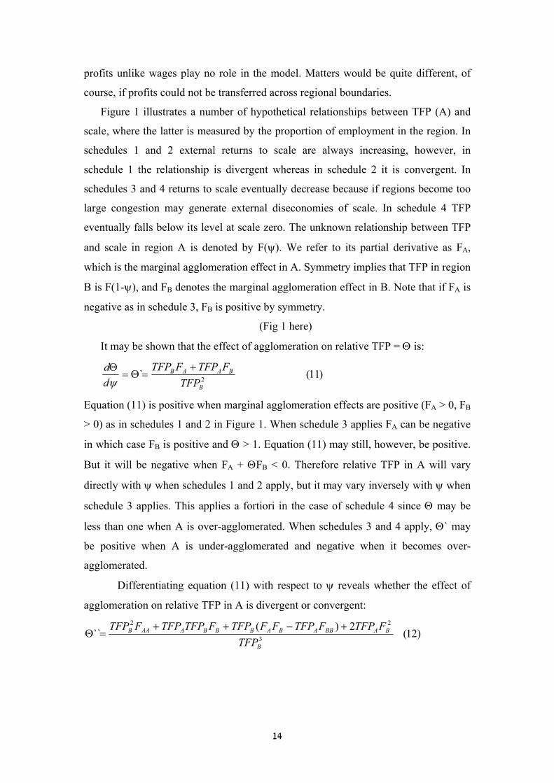
Figure 1 illustrates a number of hypothetical relationships between TFP (A) and

scale, where the latter is measured by the proportion of employment in the region. In

schedules 1 and 2 external returns to scale are always increasing, however, in

schedule 1 the relationship is divergent whereas in schedule 2 it is convergent. In

schedules 3 and 4 returns to scale eventually decrease because if regions become too

large congestion may generate external diseconomies of scale. In schedule 4 TFP

eventually falls below its level at scale zero. The unknown relationship between TFP

and scale in region A is denoted by F(ψ). We refer to its partial derivative as FA,

which is the marginal agglomeration effect in A. Symmetry implies that TFP in region

B is F(1-ψ), and FB denotes the marginal agglomeration effect in B. Note that if FA is

negative as in schedule 3, FB is positive by symmetry.

(Fig 1 here)

It may be shown that the effect of agglomeration on relative TFP = Θ is:

)11(` 2B

BAAB

TFPFTFPFTFP

dd +

=Θ=Θψ

Equation (11) is positive when marginal agglomeration effects are positive (FA > 0, FB

> 0) as in schedules 1 and 2 in Figure 1. When schedule 3 applies FA can be negative

in which case FB is positive and Θ > 1. Equation (11) may still, however, be positive.

But it will be negative when FA + ΘFB < 0. Therefore relative TFP in A will vary

directly with ψ when schedules 1 and 2 apply, but it may vary inversely with ψ when

schedule 3 applies. This applies a fortiori in the case of schedule 4 since Θ may be

less than one when A is over-agglomerated. When schedules 3 and 4 apply, Θ` may

be positive when A is under-agglomerated and negative when it becomes over-

agglomerated.

Differentiating equation (11) with respect to ψ reveals whether the effect of

agglomeration on relative TFP in A is divergent or convergent:

)12(2)(`` 3

22

B

BABBABABBBAAAB

TFPFTFPFTFPFFTFPFTFPTFPFTFP +−++

=Θ

15

where FAA and FBB denote the effects of agglomeration in A on the marginal

agglomeration effects19 in regions A and B respectively. If Θ` > 0 and Θ`` < 0

agglomeration in A has a monotonic and convergent effect on relative TFP in A. If,

however, Θ`` > 0 agglomeration in A has a divergent effect. A further possibility is

that Θ`` is positive over some range of ψ and then becomes negative. Since there may

be sign reversal in Θ` and Θ`` there is a rich taxonomy in the relationship between

relative TFP and scale.

Michel et al (1996) assume that TFPA = exp(aψ) in which case external returns

to scale are always increasing and agglomeration induces divergence in relative TFP

since:

)13(0`2``

)13(0)]1(2exp[

)exp(2`

ba

aa

aa

>Θ=Θ

>−

=Θψ

This choice of functional form naturally induces corner solutions and complete

agglomeration. To generate interior solutions Michel et al assume that unskilled labor

is completely immobile. Together with the Inada condition this constitutes a deus ex

machina that rules out complete agglomeration.

Another possible specification of F(ψ) follows equation (7) and assumes that TFP

is quadratic in scale, i.e. F(ψ) = a + bψ – cψ2. Here too we choose this specification

for reasons of convenience, flexibility and analytical tractability. Scale effects are

beneficial in A and adverse in B when ψ < b/2c, and adverse in A and beneficial in B

when ψ > b/2c. This specification implies schedule 3 in Figure 1 if b > c and it

implies schedule 4 if b < c. It also implies:

)14())1((2

)(` 22

B

b

TFPca

cb+−−

−=Θψψ

Since the maximum value of ψ(1 - ψ) = ¼ equation (14) is positive when b > c and

negative otherwise.

In summary, the effect of agglomeration in A on relative TFP may be positive

or negative, and it may be divergent or convergent. If negative Marshallian

externalities are ruled out Θ` is positive, but the sign of Θ`` is ambiguous. Finally,

19 FAA is the derivative of FA with respect to ψ and FBB is the derivative of FB with respect to 1-ψ.

16

from equation (10) the marginal effect of agglomeration in region A on relative wages

in A is equal to:

)15(`1

1` 1 ΘΘ−

== −αα

αψR

ddR

The sign of equation (15) depends directly on the sign of Θ`. This process is divergent

when:

)16(0```11

``1

>

Θ+

ΘΘ

−−Θ

=−

αα

α

αα

R

Equation (16) shows that if Θ` > 0 and Θ`` > 0 then relative wages in A are divergent

in agglomeration, which happens when agglomeration increases relative TFP

divergently. Note that if agglomeration increases relative TFP convergently, i.e. Θ` >

0 and Θ`` < 0, R`` may still be positive, in which case agglomeration has a positive

and divergent effect on A's relative wages. Therefore convergence in relative

productivity does not guarantee convergence in relative wages. If R``< 0 then relative

wages are convergent.

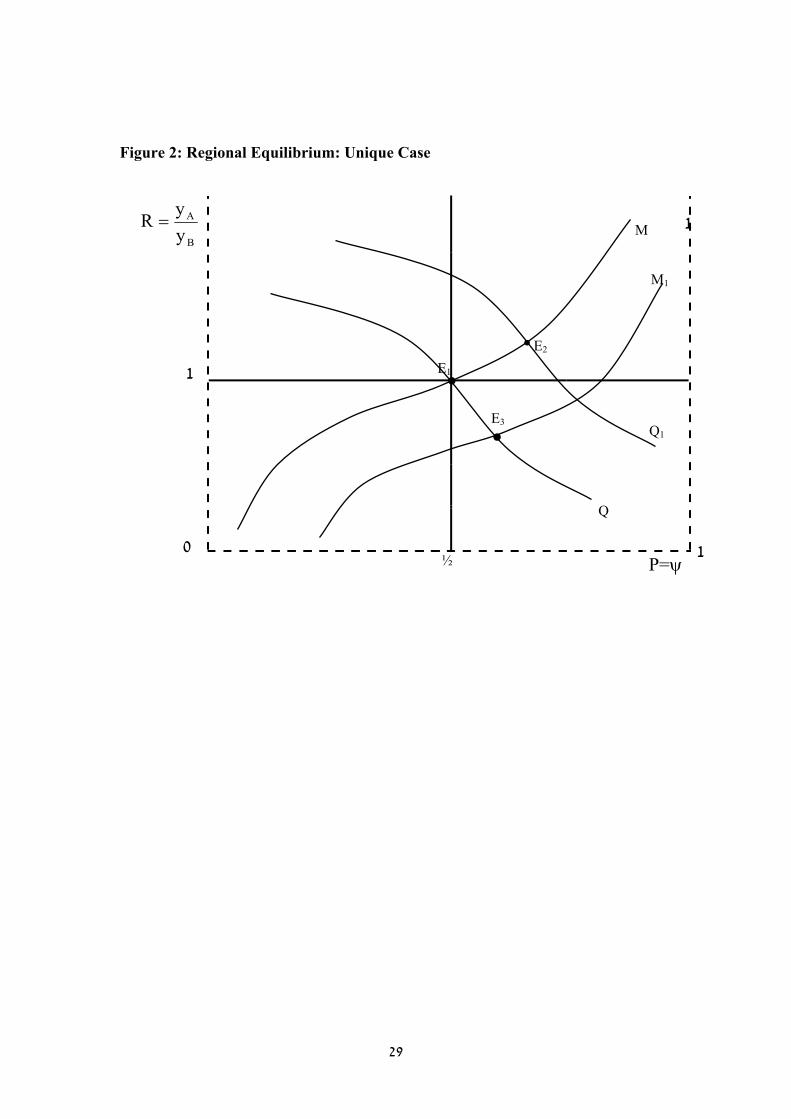
3. Regional Equilibrium

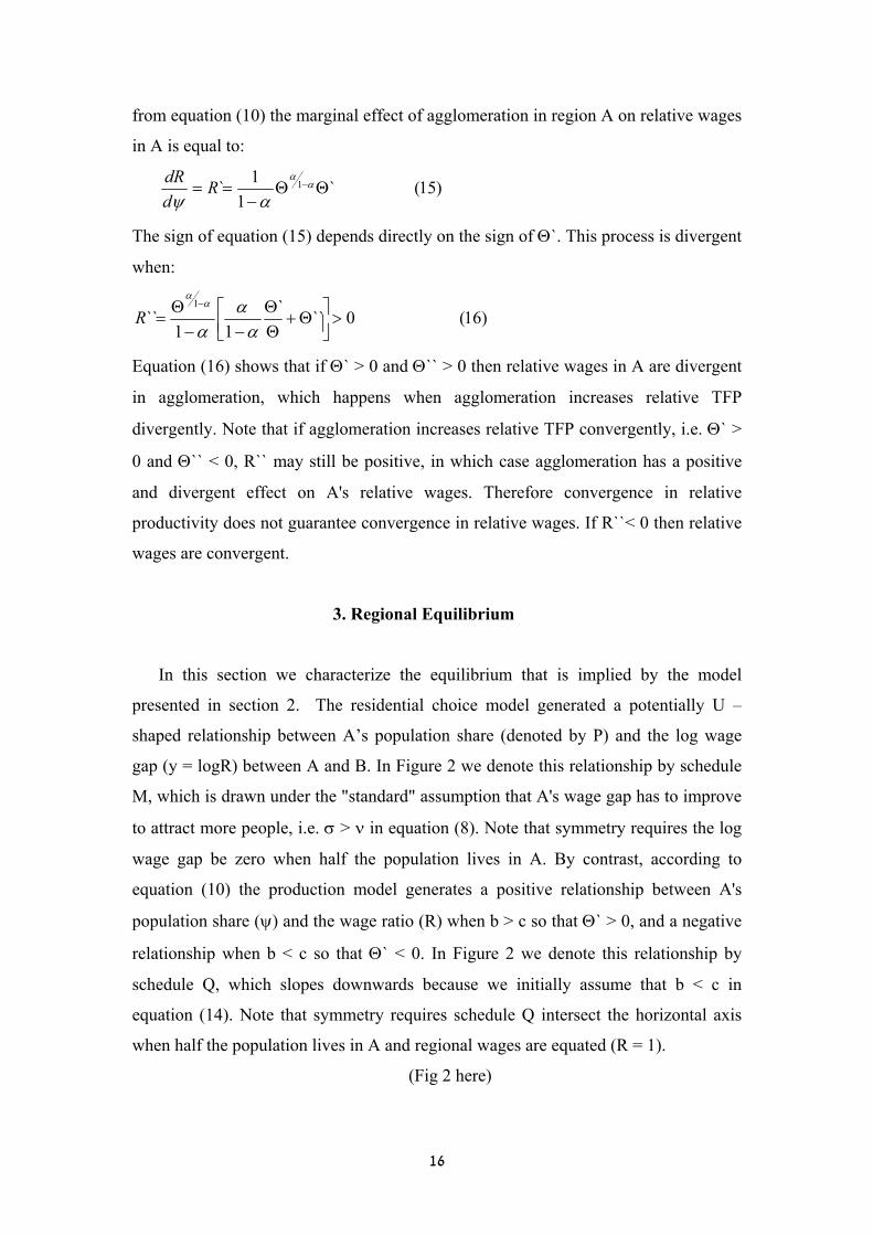
In this section we characterize the equilibrium that is implied by the model

presented in section 2. The residential choice model generated a potentially U –

shaped relationship between A’s population share (denoted by P) and the log wage

gap (y = logR) between A and B. In Figure 2 we denote this relationship by schedule

M, which is drawn under the "standard" assumption that A's wage gap has to improve

to attract more people, i.e. σ > ν in equation (8). Note that symmetry requires the log

wage gap be zero when half the population lives in A. By contrast, according to

equation (10) the production model generates a positive relationship between A's

population share (ψ) and the wage ratio (R) when b > c so that Θ` > 0, and a negative

relationship when b < c so that Θ` < 0. In Figure 2 we denote this relationship by

schedule Q, which slopes downwards because we initially assume that b < c in

equation (14). Note that symmetry requires schedule Q intersect the horizontal axis

when half the population lives in A and regional wages are equated (R = 1).

(Fig 2 here)

17

The equilibrium in Figure 2 is determined where schedules M and Q intersect,

i.e. when the supply of people choosing to reside in regions A and B is equal to firms’

demand for labor in A and B. The equilibrium condition is P = ψ. Schedules M and Q

have a single intersection at E1 at which wages are equated, and due to symmetry, half

the population is in region A. The equilibrium at E1 is stable and unique. To see this,

suppose that there was in-migration to A such that P > ½. This would drive down

wages in A relative to B's wages, which would induce reverse migration, thereby

restoring the equilibrium to E1. If there is an autonomous increase in productivity in

A, schedule Q would shift to the right (to Q1) and the new equilibrium would be at a

point such as E2, at which the wage gap opens in favor of A, and A's population share

increases. If there is an autonomous increase in residential preference in favor of A,

schedule M would shift to the right (to M1) and the new equilibrium would be at a

point such as E3, at which the wage gap opens in favor of B and A's population share

increases.

Had there been perfect inter-regional labor mobility schedule M would have been

a horizontal line emanating from 1 on the vertical axis. In the absence of scale effects

in production schedule Q would also have been a horizontal line emanating from 1 on

the vertical axis20. In this case regional wages are always equated regardless of the

population shares because capital mobility ensures that the marginal productivity of

capital is equated across regions. If there are no scale effects in production but people

have residential preferences, schedule M would be as drawn in Figure 2 and schedule

Q would be horizontal at zero, so that the wages are equated and half the population

lives in A.

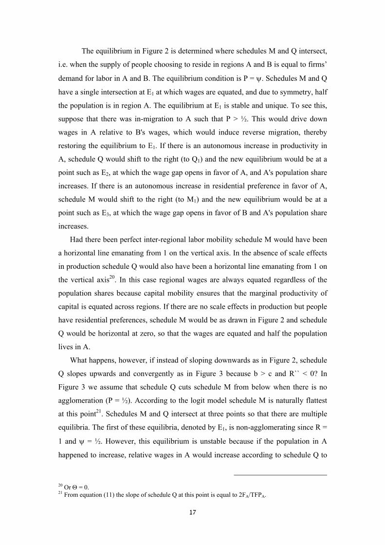
What happens, however, if instead of sloping downwards as in Figure 2, schedule

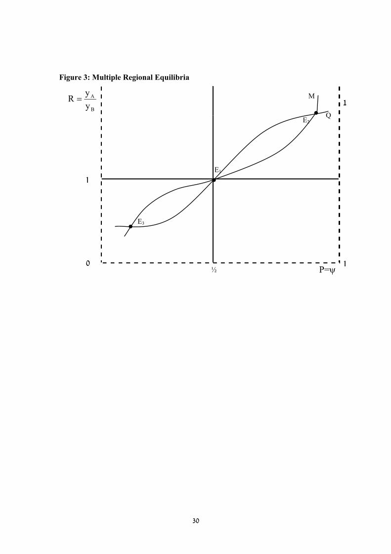
Q slopes upwards and convergently as in Figure 3 because b > c and R`` < 0? In

Figure 3 we assume that schedule Q cuts schedule M from below when there is no

agglomeration (P = ½). According to the logit model schedule M is naturally flattest

at this point21. Schedules M and Q intersect at three points so that there are multiple

equilibria. The first of these equilibria, denoted by E1, is non-agglomerating since R =

1 and ψ = ½. However, this equilibrium is unstable because if the population in A

happened to increase, relative wages in A would increase according to schedule Q to

20 Or Θ = 0. 21 From equation (11) the slope of schedule Q at this point is equal to 2FA/TFPA.

18

such an extent that yet more inward migration in A's favor would take place. This

happens because schedule Q lies above schedule M over the relevant range. This

process converges to an agglomerating equilibrium at E2 where schedules M and Q

intersect. Its symmetrical counterpart is E3, which is also stable. Therefore, stable

equilibria require that schedule M intersects schedule Q from below.

(Fig 3 here)

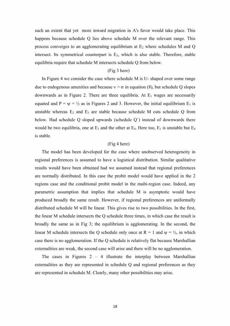
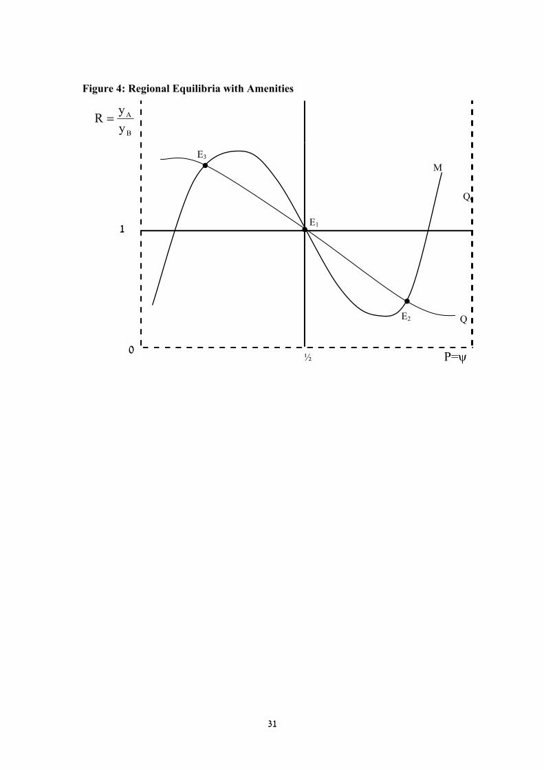
In Figure 4 we consider the case where schedule M is U- shaped over some range

due to endogenous amenities and because ν > σ in equation (8), but schedule Q slopes

downwards as in Figure 2. There are three equilibria. At E1 wages are necessarily

equated and P = ψ = ½ as in Figures 2 and 3. However, the initial equilibrium E1 is

unstable whereas E2 and E3 are stable because schedule M cuts schedule Q from

below. Had schedule Q sloped upwards (schedule Q`) instead of downwards there

would be two equilibria, one at E1 and the other at E4. Here too, E1 is unstable but E4

is stable.

(Fig 4 here)

The model has been developed for the case where unobserved heterogeneity in

regional preferences is assumed to have a logistical distribution. Similar qualitative

results would have been obtained had we assumed instead that regional preferences

are normally distributed. In this case the probit model would have applied in the 2

regions case and the conditional probit model in the multi-region case. Indeed, any

parametric assumption that implies that schedule M is asymptotic would have

produced broadly the same result. However, if regional preferences are uniformally

distributed schedule M will be linear. This gives rise to two possibilities. In the first,

the linear M schedule intersects the Q schedule three times, in which case the result is

broadly the same as in Fig 3; the equilibrium is agglomerating. In the second, the

linear M schedule intersects the Q schedule only once at R = 1 and ψ = ½, in which

case there is no agglomeration. If the Q schedule is relatively flat because Marshallian

externalities are weak, the second case will arise and there will be no agglomeration.

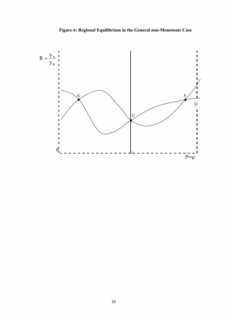
The cases in Figures 2 – 4 illustrate the interplay between Marshallian

externalities as they are represented in schedule Q and regional preferences as they

are represented in schedule M. Clearly, many other possibilities may arise.

19

4 Intergenerational Implications of the Model

The equilibria discussed in Section 3 are essentially short-term because they

refer to a single generation. In this section we discuss the intergenerational, or long

term implications of the model. The long term solution to the model differs from its

short-term counterpart for two separate reasons. First, we show that the migration

model presented in Section 2.1 implies more regional mobility between generations

than within generations. However, asymptotic mobility remains imperfectly elastic.

Secondly, if the Marshallian externalities discussed in Section 2.2 take time to

develop, they will be more pronounced in the long run than in the short run.

Recall that the "short run" lasts one generation, which is still a considerable

period of time. By contrast the “long run” may be a matter of decades or even

centuries. This recognizes the fact that agglomeration is likely to be a long and

protracted process. This should be contrasted with the speed of the agglomeration

process in models that treat internal migration in an ad hoc fashion. For example,

Michel et al assume that migration is perfectly elastic in the long run but, due to

frictions, is imperfectly elastic in the short run. This specification permits regional

wage disparities in the short run but eliminates them in the long run. The speed of the

agglomeration process depends in their case on the rate of internal migration as a

function of regional wage disparities. In the absence of frictions, the agglomeration

process would be infinitely rapid. The microfoundations underpinning these frictions

are unclear, yet they play a key role in determining the speed of the agglomeration

process, which in any case has been left vague.

By contrast, internal migration in our model is underpinned by

microfoundations and the biological clock of the agglomeration process has a

generational tick. This stems from the assumption that individuals make one major

location decision during their lifetime. In our model internal migration is therefore an

intergenerational phenomenon rather an intragenerational phenomenon as in Fujita

and Thisse. We could relax the restriction that individuals make only one major

location decision during their lifetime in which case internal migration would be both

an intergenerational and intragenerational phenomenon. But we would never expect

labor to move as freely as capital since capital is footloose, but people have ties to

their location. Since intergenerational migration is greater than intragenerational

20

migration, there is more scope for agglomeration in our model than in models which

are essentially designed for a single generation.

In Section 2.1 we pointed out that in the initial equilibrium at time

(generation) t = 0 PAA = 1/[1+exp(-φD)] and PBA = 1/[1+exp(φD)]. Consider what

happens to P1 (A's population share at t = 1) following an increase in PBA (or PAA)

induced by an autonomous increase in income in A relative to B. Assuming, for

expositional purposes, that PAA and PBA are fixed and therefore have no time indices,

the model in Section 2.1 implies the following first-order difference equation for A's

population share:

)17()( 1 BAtBAAAt PPPPP +−= −

the general solution for which is:

)19(*

)18(*)(* 0

BAAB

BA

BAAA

tt

PPPP

PPPPPP

+=

−=−+=

λλ

Since PAA > PBA it follows that 0 < λ < 1. P* denotes A's asymptotic or long run

population share. Equation (19) states that A's long run population share varies

directly with PBA and inversely with PAB. Equation (18) states that A's population

share converges upon P*.

From equation (17) the short run effect of an increase in PBA is equal to 1 – P0

= ½. Therefore, if more B residents migrate to A, A's population share increases by

half the change in PBA. To obtain the long run effect we differentiate equation (19)

with respect to PBA:

)20()(

*2

BAAB

AB

BA PPP

PP

+=

∂∂

In the symmetric case when PAB = PBA equation (20) simplifies to 1/4PAB. Due to

home region preference PAB < ½, therefore equation (20) exceeds a half in the

symmetric case, as well as in almost all asymmetric cases22. Therefore changes in PBA

typically induce more migration in the long run than in the short run. A similar

argument applies to changes in PAB. This means that the M schedule in Fig 2 is flatter

in the long run than in the short run as indicated in Figure 5 where M denotes the

short run schedule and M* is its long run counterpart. This means that if the income

22 If e.g. PAB = 0.45, PBA must be less than 0.4987 for equation (20) > ½.

21

gap increases in favor of region A, A's population share will grow from one

generation to the next until it eventually settles down at its new long run equilibrium

determined by schedule M*.

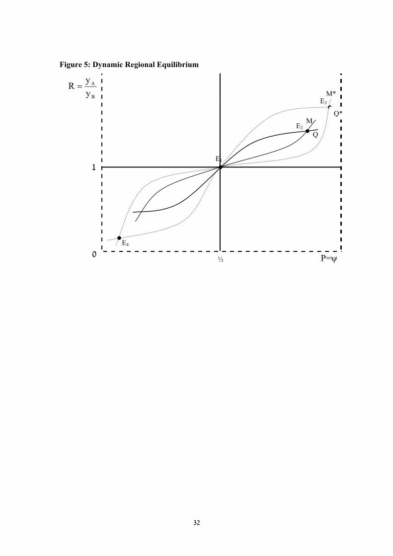
If Marshallian externalities grow over time and the Q schedule is upward

sloping as in Figure 5, the short term Q schedule will be flatter than its long term

counterpart23. This happens for any given population share because relative wages

must grow over time if Marshallian externalities are dynamic. If this process is

convergent the long run counterpart to schedule Q in Figure 5 is represented by Q*.

To formalize these dynamic externalities is difficult because relative wages

vary directly but nonlinearly with the population share according to equation (10). In

the simple first-order case R and P are related through a nonlinear difference equation

such as:

Rt = F(Rt-1, Pt) (21)

If both partial derivatives are positive, an increase in P has a greater effect on R in the

long run than in the short run, so that schedule Q* is steeper than schedule Q.

(Fig 5 here)

The short term agglomerating equilibria (E1 and E2), determined by the

intersections between schedules M and Q, have already been discussed in Figure 3.

The long run agglomerating equilibria are determined by the intersections between

schedules M* and Q* (E3 and E4). There is more agglomeration in the long run than

in the short run because schedule M* lies below schedule M when P > ½ and schedule

Q* lies above schedule Q.

Not shown in Figure 5 is the trajectory between the short and long run

equilibria, e.g. between E1 and E3. To solve the trajectory for state variables R and P it

would be necessary to substitute equation (21) into equation (17) since PAA and PBA

vary directly but nonlinearly with R. What would result is a set of second order

nonlinear difference equations in the state variables, which do not have analytical

solutions. It is obvious that A's population share and the relative wage may overshoot

their long run equilibrium at E3. And even in the absence of overshooting the

adjustment paths for the state variables may not be monotonic. Clearly many different

adjustment paths are possible. What is important for our purposes is not the

adjustment path, about which little can be said, but the fact that there must be more

23 If schedule Q slopes downwards it will be flatter.

22

agglomeration and regional wage inequality in the long run than in the short run. In

terms of Fig 5, E3 must lie to the north east of E2.

When there are more than 2 regions people face greater migration choices so

that the pull of home region preference naturally weakens24. Therefore migration in

both the short and long runs is greater in the multi-region case. When there are only 2

regions intergenerational migration is forward and backwards; if children migrate

from A to B, grandchildren migrate back to A where their grandparents live. By

contrast, in a multi-region context grandchildren may migrate onwards to regions C

and beyond. Nevertheless, while the 2 region case is restrictive, it has the virtues of

simplicity, and it serves the purpose of demonstrating that there must be more

migration intergenerationally than intragenerationally.

5. Conclusions

Although urban economists and growth theorists have attached importance to

technological spillovers, regional agglomeration theorists have focused almost

exclusively on pecuniary scale economies. We suggest that technological scale

economies may also form the basis of a theory of regional agglomeration. Our model

extends and generalizes Michel et al (1996) by focusing upon the interaction between

scale dependence in amenities and total factor productivity, and by assuming that

individuals have heterogeneous preferences regarding where they wish to live and

work. In Michel et al wage inequality depends crucially on the scale dependence of

amenities. In our model regional wage inequality arises out of heterogeneous

preferences as well as scale dependence in amenities. In the absence of scale

dependence in amenities, Michel et al (1996) are forced to assume that unskilled labor

is immobile to prevent complete agglomeration. In our model such corner solutions

are avoided more naturally by heterogeneity in residential choices. We show that

relative wages in the agglomerating region may increase under some circumstances,

but decrease under others. However, the existence of Marshallian scale externalities

do not automatically lead to regional agglomeration.

24 Variety naturally reduces the demand for individual items according to discrete choice theory since there are greater opportunities for substitution.

23

If marginal externalities are always positive there will be multiple equilibria,

and the agglomerating equilibria are stable. In the two region case it is a matter of

chance or history whether agglomeration occurs in one region rather than another. If

there is agglomeration, small shocks are self correcting, but large shocks may alter the

equilibrium. In this way ghost regions may emerge, while other regions become "hot

spots". If in addition, there are scale economies in amenities, the number of multiple

equilibria may increase. This means that shocks may not have to be so large to create

a new regional equilibrium.

We also investigated the dynamic implications of our model for

agglomeration. In doing so, we distinguish between two forces. The first concerns

dynamic effects in Marshallian externalities which may be larger in the longer run

than in the short run. The second concerns labor mobility between regions, which

according to our residential choice theory is greater between generations than within

generations. These two forces induce more agglomeration between generations than

within generation, but their implications for regional wage disparities are ambiguous.

Finally, it might be asked why do we need another theory of regional

agglomeration when NEG already exists? First, the theoretical routes taken by the two

theories are very different. There is an obvious intellectual interest when phenomena

such as regional agglomeration and regional inequality can be explained using

different and even rival axioms. Secondly, as noted by Suedekum (2006) NEG

predicts that real wages should be lower in regions that are more agglomerated. As

noted in Section 2.2 this result changes when housing is introduced into the NEG

model. Empirically, there is growing evidence that regional wages are positively

correlated with agglomeration (Beenstock and Felsenstein 2008). Our model (Figure

3) predicts that real wages should be positively correlated with agglomeration even

without the introduction of housing. However, under some circumstances this

correlation may be negative (Figure 2). Third, the empirical contents of the two

theories are very different. NEG directs empirical investigators to focus on pecuniary

scale economies and product varieties. By contrast Marshallians will direct their

empirical efforts to the determinants of regional TFP including networking and

related externalities. In the final analysis, of course, the theories have to be tested

empirically. Finally, the Marshallian model is simpler and more transparent than

NEG. It has analytical solutions whereas NEG is usually solved numerically.

24

References Abdel-Rahman, H.M. and Fujita M.(1990) Product Variety, Marshallian Externalities and City Size, Journal of Regional Science, 30(2),165-182. Abdel-Rahman, H.M. (2000) Multi-Firm City Versus Company Town: A Micro-Foundation Model of Localization Economies, Journal of Regional Science, 40 (4), 755-769. Anselin L, Varga A. and Acs Z.J. (1997) Geographic Spillovers Between University Research and High Technology Innovations, Journal of Urban Economics, 42, 422-448. Azzoni C.R. and L.M.S. Servo (2002) Education, Cost of Living and Regional Wage Inequality in Brazil, Papers in Regional Science, 81: 157-75. Baldwin R, R. Forslid, P. Martin, G. Ottaviano and F. Robert-Nicoud (2003) Economic Geography and Public Policy, Princeton University Press. Barro R.J. and X. Sala-I-Martin (1991) Convergence across States and Regions, Brookings Papers in Economic Activity, 1, 107-82. Beenstock M. and D. Felsenstein (2008) Regional Heterogeneity, Conditional Convergence and Regional Inequality, Regional Studies, 42(4), 475-488. Belleflamme P., Picard (P) and Thisse, J-F. (2000) An Economic Theory of Regional Clusters, Journal of Urban Economics, 48, 158-184. Berliant M., Reed . R.R., Wang P (2006) Knowledge Exchange, Matching, and Agglomeration, Journal of Urban Economics, (2006) 69–95. Blomquist G.C. (2006) Measuring Quality of Life, chapter 28 in R.J. Arnott and D.P. McMillen (eds) A Companion to Urban Economics, Oxford, Blackwell. Brakman S., H. Garretsen and C. van Marrewijk (2001) An Introduction to Geographical Economics, Cambridge University Press. Charlot S. and Duranton G. (2004) Communications Externalities in Cities, Journal of Urban Economics, 56, 581-613. DaVanzo J. and Morrison F. (1981) Return and Other Sequences of Migration in the US, Demography, 18, 85-101. David P.A.and Rosenbloom J.L. (1990) Marshallian Factor Market Externalities and the Dynamics of Industrial Location, Journal of Urban Economics, 28, 349-370. Dixit A.K. and Stiglitz J.E. (1977) Monopolistic Competition and Optimum Product Diversity, American Economic Review , 67(3), 297-308.

25

Duranton G. and V. Monastiriotis (2002) Mind the Gaps: the Evolution of Regional Inequalities in the UK 1982-1997, Journal of Regional Science, 42: 219-56. Evans P. and McCormick B. (1994) The New Pattern of Regional Unemployment: Causes and Policy Significance, The Economic Journal, 104 (424), 663-647. Duranton G. and Puga D. (2004) Micro-Foundations of Urban Agglomeration Economies, pp. 2064-2117 in J. V. Henderson and J.-F. Thisse (eds.), Handbook of Regional and Urban Economics, Vol. 4. Amsterdam: North Holland. Ferguson C.E. (1969) The Neoclassical Theory of Production and Distribution, Cambridge University Press. Fu S. (2007) Smart Café Cities: Testing Human Capital Externalities in the Boston Metropolitan Area, Journal of Urban Economics, 61: 86-111. Fujita M., P. Krugman and A. Venables (1999) The Spatial Economy: Cities, Regions and International Trade, MIT Press. Fujita M. and J-F Thisse (2002) Economics of Agglomeration: Cities, Industrial Location and Regional Growth, Cambridge University Press. Glaeser E.L. (1999) Learning in Cities, Journal of Urban Economics, 46, 254-277. Glaeser E.L. and Mare D.C. (2001) Cities and Skills, Journal of Labor Economics, 19(2), 316-342. Grossman G.E. and E. Helpman (1993) Innovation and Growth in the Global Economy, MIT Press. Gould E.D. and Paserman M.D. (2003). Waiting for Mr. Right: Rising Inequality and Declining Marriage Rates, Journal of Urban Economics, 53 (2), 257-281. Harcourt G. (1972), Some Cambridge Controversies in the Theory of Capital. Cambridge: Cambridge University Press. Hartman S., M.K. Doanne, and C.K. Woo (1991) Consumer Rationality and the Status Quo, Quarterly Journal of Economics, 106: 141-62. Helpman E. (1998) The Size of Regions, D. Pines, E. Sadka and I. Zilcha (eds) Topics in Public Economics: Theoretical and Applied Analysis, Cambridge University Press. Helsley R.W. and Strange W.C. (2004) Knowledge Barter in Cities, Journal of Urban Economics, 56 (2004) 327–345. Henderson J.V. (1974) The Sizes and Types of Cities, American Economic Review, 64: 640-656. Henderson J.V. (2003) Marshall's Scale Economies, Journal of Urban Economics, 53: 1-28.

26

Hicks J.R. (1932) A Theory of Wages, Macmillan, London. Jaffe A.B., Trajtenberg M. and Henderson R. (1993) Geographic Localization of Knowledge Spillovers as Evidenced by Patent Citations, Quarterly Journal of Economics, 108, 577-98. Krugman P.R. (1991) Increasing Returns and Economic Geography, Journal of Political Economy, 99: 483-99. Long L. (1991) Residential Mobility Differences Among Developed Countries, International Regional Science Review, 14 (2), 133-148. Marshall A (1919) Principles of Economics, 8th Edition, Macmillan, London. Marshall A. (1920) Industry and Trade, Macmillan, London. Jovanovic B. and R. Rob (1989) The Growth and Diffusion of Knowledge, Review of Economic Studies, 56: 569-582. Maier G. and P. Weiss (1986) The Importance of Regional Factors in the Determination of Earnings: the Case of Austria, International Regional Science Review, 10: 211-20. Michel P., A. Perrot and J-F. Thisse (1996) Interregional Equilibrium with Heterogeneous Labor, Journal of Population Economics, 9: 95-114. Murata Y. (2006) Product Diversity, Taste Heterogeneity, and Geographic Distribution of Economic Activities: Market vs. Non-Market Interactions, Journal of Urban Economics, 53: 126-144. Nocco A., (2008) Preference, Heterogeneity and Economic Geography, Journal of Regional Science, (forthcoming) Ottaviano, G. I. P., and Thisse, J-F. (2004) Agglomeration and Economic Geography, pp. 2563-2608 in J. V. Henderson and J.-F. Thisse (eds.), Handbook of Regional and Urban Economics, Vol. 4. Amsterdam: North Holland. Puga D. (1999) The Rise and Fall of Regional Inequalities, European Economic Review, 43: 303-34. Rosenthal S. and Strange W. (2004) Evidence on the Nature and Sources of Agglomeration Economies, pp. 2120-2171 in J. V. Henderson and J.-F. Thisse (eds.), Handbook of Regional and Urban Economics, Vol. 4. Amsterdam: North Holland. Storper M. and Venables A.J. (2004) Buzz: Face to Face Contact and the Urban Economy, Journal of Economic Geography, 4, 351-370. Suedekum J. (2006) Agglomeration and Regional Living Costs, Journal of Regional Science, 46: 529-43.

27

Tabuchi T. and Thisse. J-F.(2002) Taste Heterogeneity, Labor Mobility and Economic Geography, Journal of Development Economics, 69, 155-177.

28

Figure 1: The Relationship Between Scale and TFP

TFP

P

½0

1

2

3

4

29

Figure 2: Regional Equilibrium: Unique Case

B

A

y

yR =

P=ψ

1

M

Q

E2

E1

½

E3

1

M1

Q1

0 1

30

Figure 3: Multiple Regional Equilibria

B

A

y

yR =

P=ψ

E1

M

E2 Q

1

1

0

E3

1 ½

31

Figure 4: Regional Equilibria with Amenities

B

A

y

yR =

P=ψ

½

1

M

E2

E1

Q0

Q

E3

0

32

Figure 5: Dynamic Regional Equilibrium

B

A

y

yR =

P=ψ

M

E1

Q

½

E2

1

0

E4

M*E3

Q*

33

Figure 6: Regional Equilibrium in the General non-Monotonic Case

B

A

y

yR =

P=ψ

S

½

0

U

Q

S