MD SURVEY MARSHALLIAN MACROECONOMIC MODEL: A …

Macroeconomic Dynamics, 9. 2005, 220-243. Printed in the United States of America.001: 10.1017.S1365100504040180

MD SURVEY

MARSHALLIAN MACROECONOMICMODEL: A PROGRESS REPORT

ARNOLD ZELLNER AND GUILLERMO ISRAILEVICH

University of Chicago

In this progress report, we first indicate the origins and early development of theMarshallian Macroeconomic Model and briefly review some of our past empiricalforecasting experiments with the model. Then we present recently developed one-sector,two-sector and n-sector models of an economy that can be employed to explain pastexperience, predict future outcomes, and analyze policy problems. The results ofsimulation experiments with various versions of the model are provided to illustrate someof its dynamic properties that include "chaotic" features. Last, we present comments onplanned future work with the model.

Keywords: Marshallian Macroeconomic Model, Disaggregation, Prediction, Simulation,One-Sector Model, Two-Sector Model, n-Sector Model

1. ORIGINS AND EARLY DEVELOPMENT OF THE MMM

In the early 1970's, the structural econometric modeling, time-series analysis(SEMTSA) approach that provides methods for checking existing dynamic econo-metric models and for constructing new econometric models was put forward; seeZellner and Palm (1974,1975,2004), Palm (1976,1977,1983), and Zellner (1997,p. IV; 2004). In Zellner and Palm (2004), many applications of the SEMTSA ap-proach are reported, including some that began in the mid-1980's that involvedan effort by Garcia-Ferrer, Highfield, Palm, Hong, Min, Ryu, Zellner, and othersto build a macroeconometric model that works well in explaining the past, pre-diction, and policymaking. In line with the SEMTSA approach, we started themodel-building process by developing dynamic equations for individual variablesand tested them with past data and in forecasting experiments. The objective is todevelop a set of tested components that can be combined to form a model and torationalize the model in terms of old or new economic theory.

The first variable that we considered was the rate of growth of real gross domesticproduct (GDP). After some experimentation, we found that various variants of anAR(3) model, including lagged leading indicator variables-namely the rates of

Resean:h was financed in part by funds from die National Science Foundation, die CDC Invesunent ManagementCorporation, and die Alexander Endowment Fund, Graduate School of Business, University of Chicago. Addressco=spondence to: Arnold Zellner, Graduate School of Business, University of Chicago, Hyde Parlc Center, Chicago,IL 60637, USA; e-mail: [email protected]. http://gsbwww.uchicago.edu/fac/arnold.rellner/more.

220@ 2005 Cambridge University Press 1365-1005/05 $12.00

MARSHALLIAN MACRO MODEL 221

growth of real money and of real stock prices--called an autoregressive-leadingindicator (ARLI) model worked reasonably well in point forecasting and turningpoint forecasting experiments using data first for 9 industrialized countries andthen for 18 industrialized nations. Later, a world income variable, the mediangrowth rate of the 18 countries' growth rates was introduced in each country'sequation and an additional ARLI equation for the median growth rate was addedto give us our ARLI/WI model. The variants of the ARLI and ARLI/WI modelsthat we employed included fixed-parameter and time-varying parameter state-space models. Further, Bayesian shrinkage ~d model-combining techniques wereformulated and applied that produced gains in forecasting precision. See Zellnerand Palm (2004) and Zellner (1997, p. IV) for empirical results. It was found thatuse of Bayesian shrinkage techniques produced notable improvements in forecastprecision and in turning-point forecasting with about 70% of 211 turning-pointepisodes forecasted correctly; see Zellner and Min (1999).

Given these ARLI and ARLI/WI models that worked reasonably well in fore-casting experiments using data for 18 industrialized countries, the next step inour work was to rationalize these models using economic theory. It was foundpossible to derive our empirical forecasting equations from variants of an aggre-gate demand and supply model in Zellner (2000). Further, Hong (1989) derivedour ARLI/WI model from a Hicksian IS-LM macroeconomic theoretical modelwhile Min (1992) derived it from a generalized real-business-cycle model thathe formulated. Although these results were satisfying, it was recognized that theroot mean squared errors of the models' forecasts of annual growth rates of realGDP, in the vicinity of 1.7 to 2.0 percentage points, while similar to those of someOECD macroeconometric models, were rather large. Thus, we thought about waysto improve the accuracy of our forecasts.

In considering this problem, it occurred to us that perhaps using disaggregateddata would be useful. For an example illustrating the effects of disaggregationon forecasting precision, see Zellner and Tobias (2000). The question was howto disaggregate. After much thought and consideration of ways in which oth-ers, including Leontief, Stone, Orcutt, the Federal Reserve-MIT-PENN modelbuilders, had disaggregated, we decided to disaggregate by industrial sectors andto use Marshallian competitive models for each sector. In earlier work by Veloceand Zellner (1985), a Marshallian model of the Canadian furniture industry wasformulated to illustrate the importance of including not only demand and supplyequations in analyzing industries' behavior but also an entry/exit relation. It waspointed out that on aggregating supply functions over producers, the industrysupply equation includes the variable, the number of firms in operation at time t,N(t). Thus, there are three endogenous variables in the system, price p(t), quantityq(t), and N(t), and, as Marshall emphasized, the process of entry and exit of firmsis instrumental in producing a long-run, zero-profit industry equilibrium. Further,given that producers were assumed to be identical, profit maximizers with Cobb-Douglas production functions and selling in competitive markets with "log-log"demand functions and a partial-adjustment entry/exit relation, it was not difficult

222 ARNOLD ZELLNER AND GUILLERMO ISRAILEVICH

to solve the system for a reduced-form equation for industry sales. As will beshown below, this system yielded a reduced-form logistic differential equationfor industry sales, including a linear combination of "forcing" variables, namely,rates of growth of exogenous variables that affect demand and supply (e.g., realincome, real factor prices and real money).

Given this past work on a sector model of the Canadian furniture industry, itwas thought worthwhile to consider similar models, involving demand, supply,and entry/exit relations for various sectors of the U.S. economy, namely, agricul-ture, mining, construction, durables, whole,sale, retail, etc., and to sum forecastsacross sectors to get forecasts of aggregate variables. Whether such "disaggregate"forecasts of aggregate variables would be better than forecasts of the aggregatevariables derived from aggregate data was a basic issue. Earlier, these aggregation!disaggregation issues had been considered by many, including Zellner (1962),Liitkepohl (1986) and de Alba and Zellner (1991), with the general analyticalfinding that many times, but not always, it pays to disaggregate. In addition, wewere quite curious about whether inclusion of entry/exit relations in our modelthat do not appear generally in other macroeconomic models would affect its

performance.To summarize some of the positive aspects of disaggregation by sectors of

an economy, note that these sectors, for example, agriculture, mining, durables,construction, and services, exhibit very different seasonal, cyclical, and trendbehavior and that there is great interest in predicting the behavior of these im-portant sectors. Further, sectors have relations involving both sector-specific andaggregate variables, with the sector-specific variables (e.g., prices, weather) givingrise to sector-specific effects. Since sector relations have error terms with differingvariances and that are correlated across sectors, it is possible not only to use jointestimation and prediction techniques to obtain improved estimation and predictiveprecision but also to combine such techniques with the use of Stein-like shrink-age techniques to produce improved estimates of parameters and predictions ofboth sector and aggregate variables. In the literature, such approaches have beenimplemented successfully using time-varying parameter, state-space models toallow for possible "structural breaks" and other effects leading to parameters'values changing through time. See, Zellner et al. (1991) and Quintana et al. (1997)for examples of such applied analyses, the former in connection with predictingoutput growth rates and turning points in them for 18 industrialized countries andthe latter in connection with formation of stock portfolios utilizing multivariatestate-space models for individual stock returns, predictive densities for futurereturns, and Bayesian portfolio formation techniques.

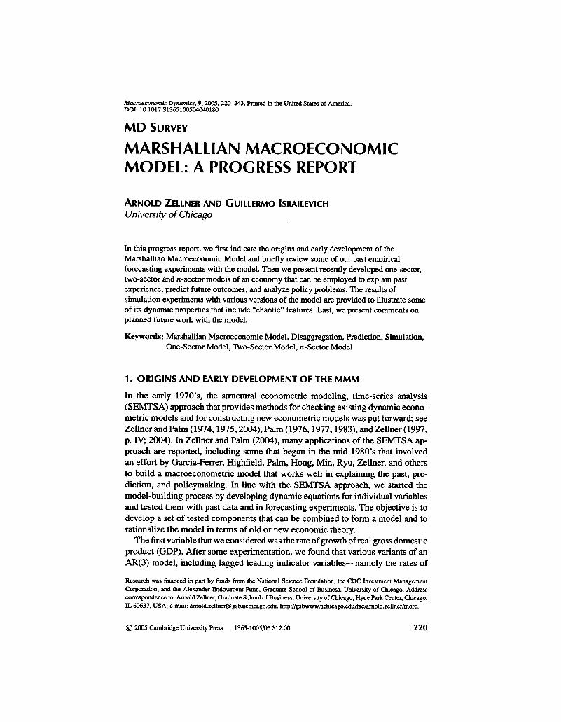
To illustrate some of the points made in the preceding paragraph, in Figure 1,taken from Zellner and Chen (2001), the annual output growth rates of 11 sectorsof the U.S. economy, 1949-1997, are plotted. It is evident that sectors' growth ratesbehave quite differently. For example, note the extreme volatility of the growthrates of agriculture, mining, durables, and construction; see the box plots presentedin Zellner and Chen (2001, Fig. 1 C) paper for further evidence of differences in


1950 1955 1990 19951960 1965 1970 1975 1980 1985

FIGURE 1. U.s. sectoral real output growth rates.

dispersion of growth rates across sectors. Also, it is clearly the case that sectoroutput growth rates are not exactly synchronized. With such disparate behavior ofgrowth rates of different sectors, much information is lost in using aggregate dataand models for forecasting and policy analysis.

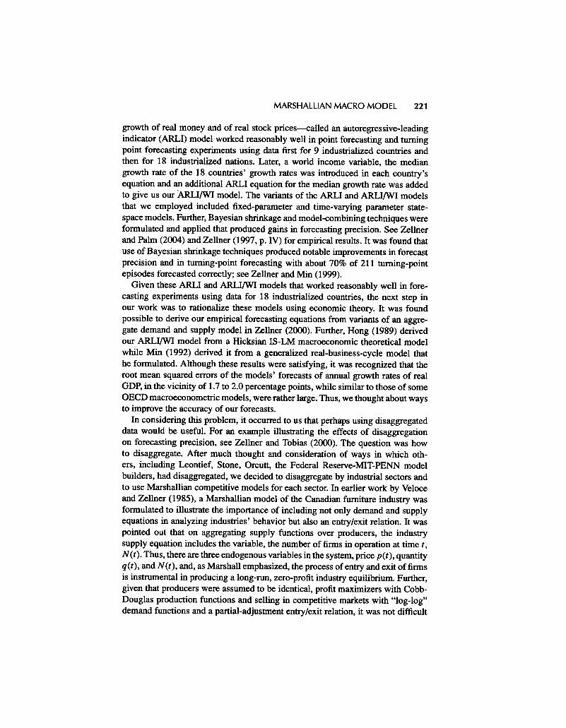
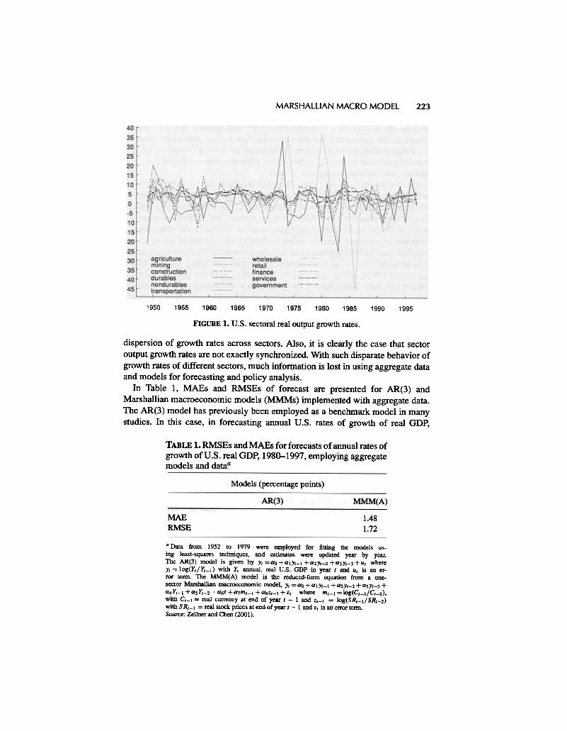
In Table 1, MAEs and RMSEs of forecast are presented for AR(3) andMarshallian macroeconomic models (MMMs) implemented with aggregate data.The AR(3) model has previously been employed as a benchmark model in manystudies. In this case, in forecasting annual U.S. rates of growth of real GDP,

TABLE 1. RMSEs and MAEs for forecasts of annual rates ofgrowth of U.S. real GDP, 1980-1997, employing aggregatemodels and dataa

Models (percentage points)

MAERMSE

1.481.72

.Data from 1952 to 1979 were employed for fitting the models us-ing least-squares techniques, and estintates were updated year by year.The AR(3) model is given by Yt=aO+alYt-l+a2Yt-2+a3Yt-3+U, whereYt = log(Yt/Yt-l) with Yt annual, real U.S. GDP in year t and Ut is an er-ror term. The MMM(A) model is the reduced-form equation from a one-sector Marsha11ian macroeconomic model, Yt =ao +alYt-l +a2Yt-2 +a3Yt-3 +a4Yt-l+asYt-2+a6t+a7mt-l+aSZt-l+Bt where mt-l=log(Ct-I/Ct-2),with C'-l = real currency at end of year t -I and Zt-l = log(SRt-l/SR,-vwith SRt-l = real stock prices at end of year t -I and Bt is an error term.Source: Zellner and Chen (2001).


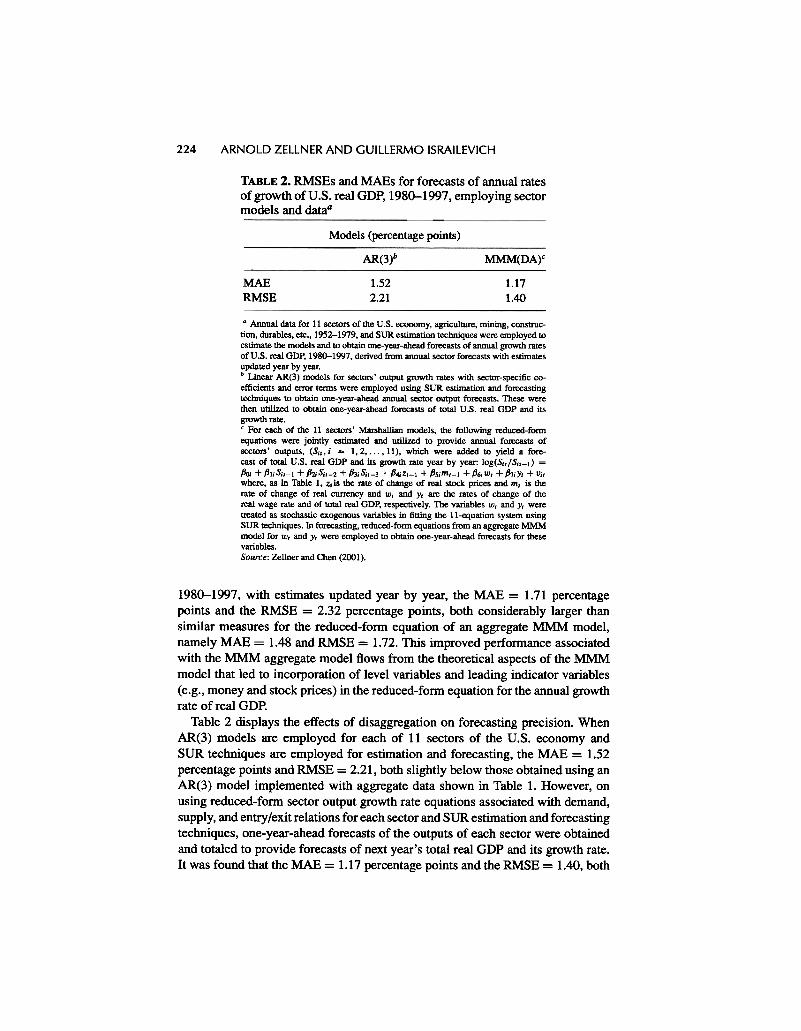
TABLE 2. RMSEs and MAEs for forecasts of annual ratesof growth of U.S. real GDP, 1980-1997, employing sectormodels and dataQ

Models (percentage points)

AR(3)b MMM(DA)C

MAERMSE

1.522.21 1.171.40

.Annual data for 11 sectors of the U.S. economy, agriculture, mining, construc-tion, durab1es, etc., 1952-1979, and SUR estimation techniques were employed toestimate the models and to obtain one-year-ahead forecasts of annual growth ratesof U.S. real GDP, 1980-1997, derived from annual sector forecasts with estimates

updated year by year.b Linear AR(3) models for sectors' output growth rates with sector-specific co-

efficients and error terms were employed using SUR estimation and forecastingtechniques to obtain one-year-ahead annual sector output forecasts. These werethen utilized to obtain one-year-ahead forecasts of total U.S. real GDP and itsgrowth rate.C For each of the 11 sectors' Marshallian models, the following reduced-form

equations were jointly estimated and utilized to provide annual forecasts ofsectors' outputs, (Sit, i = 1,2,...,11), which were added to yield a fore-cast of total U.S. real GDP and its growth rate year by year: log(Sit/Sit-U =

.801 + {JliSit-1 + /l2iSit-2 + {J3iSit-3 + {J4iZt-l + {JSimt-1 + {J6iWt + fJOJiYt + Vitwhere, as in Tahle I, Ztis the rate of change of real stock prices and mt is therate of change of real currency and Wt and Yt are the rates of change of thereal wage rate and of total real GDP, respectively. The variables Wt and Yt weretreated as stochastic exogenous variables in fitting the II-equation system usingSUR techniques. In forecasting, reduced-form equations from an aggregate MMMmodel for Wt and Yt were employed to obtain one-year-ahead forecasts for thesevariables.Source: Zellner and Chen (2001).

1980-1997, with estimates updated year by year, the MAE = 1.71 percentagepoints and the RMSE = 2.32 percentage points, both considerably larger thansimilar measures for the reduced-fOnD equation of an aggregate MMM model,namely MAE = 1.48 and RMSE = 1.72. This improved perfonnance associatedwith the MMM aggregate model flows from the theoretical aspects of the MMMmodel that led to incorporation of level variables and leading indicator variables(e.g., money and stock prices) in the reduced-fonD equation for the annual growthrate of real GDP.

Table 2 displays the effects of disaggregation on forecasting precision. WhenAR(3) models are employed for each of 11 sectors of the U.S. economy andSUR techniques are employed for estimation and forecasting, the MAE = 1.52percentage points and RMSE = 2.21, both slightly below those obtained using anAR(3) model implemented with aggregate data shown in Table 1. However, onusing reduced-fonD sector output growth rate equations associated with demand,supply, and entry/exit relations for each sector and SUR estimation and forecastingtechniques, one-year-ahead forecasts of the outputs of each sector were obtainedand totaled to provide forecasts of next year's total real GDP and its growth rate.It was found that the MAE = 1.17 percentage points and the RMSE = 1.40, both


of which are considerably smaller than those for the MMM aggregate forecasts,MAE = 1.48 and RMSE = 1.72 and for the AR(3) model. Thus, in this case,use of the MMM's theory along with disaggregation has resulted in improvedforecasting performance. For more results based on other methods and variants ofthe MMM, see Zellner and Chen (2001).

These positive empirical results encouraged us to proceed to analyze the prop-erties of our m'odels further and to add factor markets and a government sector toclose the model. Further, we discovered that discrete versions of our MMM arein the form of chaotic models that, as is wetl known, have solutions with a widerange of possible forms, depending on values of parameters and initial conditions.

2.

DEVELOPMENT OF A COMPLETE ONE-SECTOR MMM

In this section, we indicate how to formulate a complete one-sector MMM. Ex-tending the work of Veloce and Zellner (1985) and Zellner (2001), we introducedemand, supply, and entry/exit equations. The supply equation is derived by aggre-gating the supply functions of individual, identical, competitive, profit-maximizingfirms operating with Cobb-Douglas production functions. Further, firms' factordemand functions for labor and capital services are aggregated over firms to obtainmarket factor demand functions. Given a demand function for output and factorsupply functions for labor and capital services, we have a complete one-sector,seven-equation MMM. Further, with the introduction of government and moneysectors, an expanded one-sector MMM model with government and money isobtained and is described below. Results of some simulation experiments withthese models are presented and discussed.

2.1. Product Market Supply, Demand, and Entry/Exit Equations

We assume a competitive Marshallian industry with N = N(t) firms in operationat time t, each with a Cobb-Douglas production function, q = A * La K fJ, where

A* = A*(t) = AN(t)AL(t)AK(t), the product of a neutral technological change

factor and labor and capital augmentation factors that reflect changes in the quali-ties of labor and capital inputs. Later, we introduce money services as another factorinput. Additional inputs, for example, raw materials and inventory service inputs,can be added without much difficulty. The production function exhibits decreasingreturns to scale with respect to labor and capital. This could be interpreted as theresult of missing factors, for example, entrepreneurial skills that are not includedin the model. Note that our Cobb-Douglas production function with decreasingreturns to scale, combined with fixed entry costs introduced below, yields a U-shaped long-run average cost function. Given the nominal wage rate w = w(t),the nominal price for capital services r = r(t), and the product price p =p(t), and assuming profit maximization, the sector's nominal sales supply func-tion is S = N Apl/6w-a/6r-fJ/6, where A = A*I/6, and 0 < f) = 1- a -f3 < 1.On logging both sides of the equation for nominal sales S, and differentiating with


respect to time, we obtain the industry nominal sales equation

S/S = N /N + A/A + (l/fJ)p/p -(a/fJ)w/w -({J/fJ)r/r (Product Supply),

(1)

where xix = (1/x)dxldt. Note that with no entry or exit (Iv I N = 0) and no tech-nical change (AI A = 0), an equal proportionate change in the prices for productand for factors will not affect real sales. That is, from (1), SI S -pip = O.

On multiplying both sides of the industry output demand function by p, weobtain an expression for nominal sales, S ~ pQ = Bpl-'1Y'18 H'1hX{l Xi2.. .XJd,where Y is nominal disposable income, H is the number of households, and the xvariables are demand shift variables such as money balances, demand trends, etc.On logging and differentiating this last equation with respect to time, the result is

d

S/S = (1 -7])p/p + 7]sS/S + 7]hH/H + L 7]jXj/Xjj=1

(Product Demand).

(2)

In a one-sector economy without taxes, we can replace nominal disposableincome Y with nominal sales S. Ceteris paribus, an equal change in prices andnominal income will not affect real demand. That is, from (2), S I S -jJ I p = 0,provided that 17 = 179' implying no money illusion. Note that money illusion mightarise from psychological reasons and/or systematic lack of information regardingrelative prices and systematic errors in anticipations. Also, equation (2) can beexpanded to include costs of adjustment, habit persistence, and expectation effects.

The following entry/exit equation completes the product market model:

N IN = y'(n -Fe) = y(S -F) (Entry/Exit) (3)

with nominal profits given by n = 9S used in going from the first equal-ity to the second in (3). Also in going from the first equality to the second,F = F(t) = Fe(t)j9, with Fe(t) the equilibrium level of profits at time t takingaccount of discounted entry costs and y = y'9, with y = y(t) and y' = y'(t). Suchfixed costs make the long-run average cost function U -shaped for a firm operatingwith decreasing returns to scale, as assumed above. Equation (3), with y = y(t),where t is time, represents firm entry/exit behavior as a time-varying function ofindustry profits relative to the equilibrium level of profits. Further, equation (3)can be elaborated to take account of possible asymmetries, expectations, and lagsin entry and exit behavior. For example, exit may not occur immediately if fixedcosts incorporated in Fe are sunk.

2.2. Factor Market Demand and Supply Equations

Now we extend the model to include demand and supply equations for labor andcapital. From assumed profit maximization, with N competitive firms operating


with Cobb-Douglas production functions, as described above, the aggregate de-mandfor labor input is L = aNpqjw = aSjw. Similarly, the aggregate demandfor capital services is K = fJNpqjr = fJSjr. Logging and differentiating theselast two equations with respect to time, we obtain

(Labor Demand) (4)

(Capital Demand). (5)

As regards labor supply, we assume L=D(wjp)O(Yjp)o'HohZflZ~2...Z:1.

Also, with respect to capital service supply, we assume K=E(rjp)"'(Yj

p )"'. H"'h Vfl vt ...vtk where the z and v variables are "supply shifters." As before,

we replace nominal income by nominal sales, and logging and differentiating with

respect to time, we obtain

LjL = SjS -IiJjw

KjK = SjS -fjr

LIL = b'(wlw -pip) + b's(SIS -pip) +b'hHIHI

+ Lb'izilzi (Labor Supply),i=1

(6)

K/K = tP(f/r -pip) + tPs(s/s -pip) +tPhH/Hk

+ L tPiVi/Vi (Capital Supply).i=l

(7)

Above, Ii / H is the rate of change of the number of households.The above seven-equation model is complete for the seven endogenous variables

N, L, K, p, w, r, and S with the variables H, A*, y', Fe, x, z, and V assumedexogenously determined. The model can be solved analytically (see Appendix Afor details) for the reduced-form equation for S / S that is given by

SjS = a(S -F) + bg, (8)

where a and b are parameters and g is a linear function of the rates of change ofthe exogenous variables given above. If a, b, F, and g have constant values, (8)is the differential equation for the well-known and widely used logistic function.Further, if g = g(t), a given function of time, as noted by Veloce and Zellner (1985,p. 463) the equation is a variant ofBemoulli's differential equation. Note that g maychange through time because of changes in the rates of growth of technologicalfactors, households, etc.; for an explicit expression for g(t), see equation (A.5) inAppendix A. Further, the logistic equation in (8) can be expressed as

dS= klS[1 -(k2/k1)S]

dtwhere k1 = (g -y F)/(1 -f) and k2 = -y/(1 -f).

The solution to (9) is given by S(t) = (k1/ kV/[1 -ce-klt] where c = (1 +k1/ k2So) with So the initial value. Also, from (9), it is seen that there are two

(9)


equilibrium values, namely, S = 0 and S = k1/k2, with the fonner unstable for

positive values of the k parameters. Note that for constant values of the parameters,(9) cannot generate cyclical movements. However, if the parameters are allowedto vary, the output of (9) can be quite variable. Further, in some cases, there may bea discrete lag in (9) and then the equation becomes a mixed differential-differenceequation that can have cyclical solutions; see, for example, Cunningham (1958).Whether the economy is best modeled using continuous-time, discrete-time, ormixed models is an open issue that deserves further theoretical and empiricalattention.

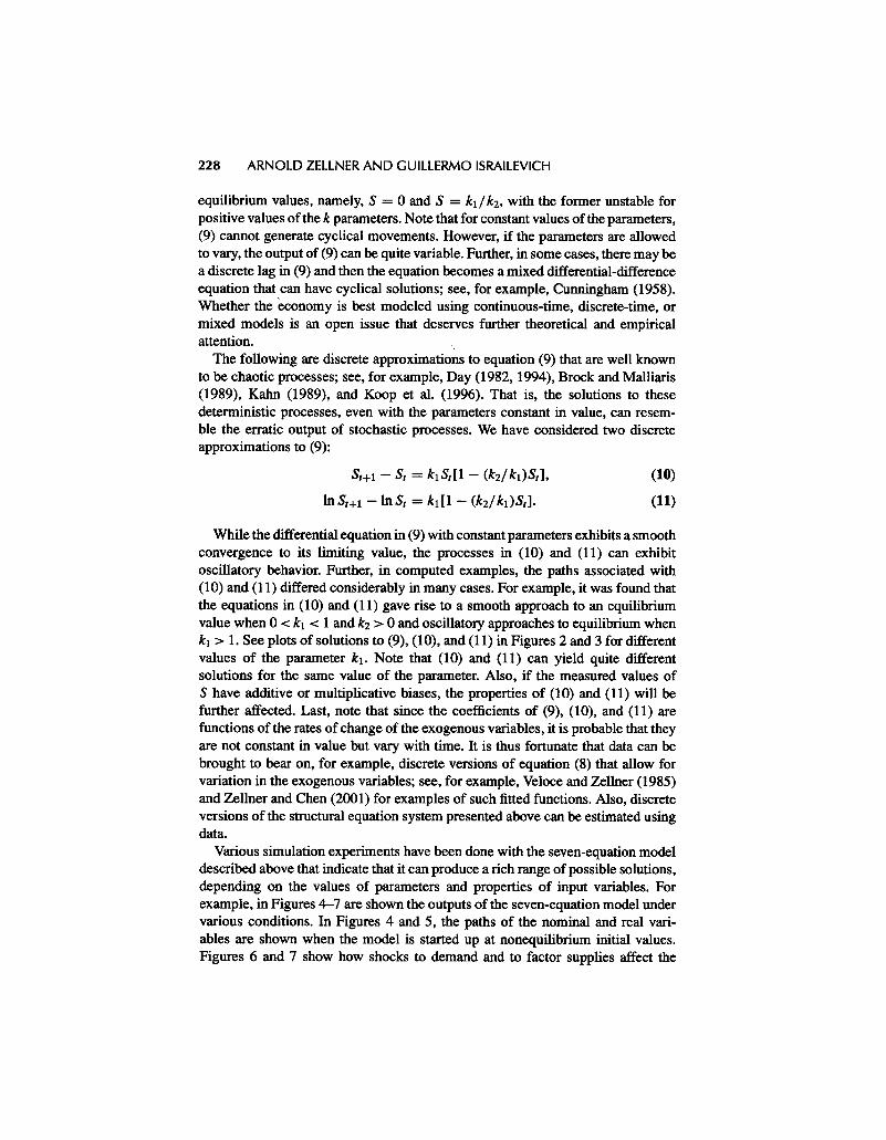
The following are discrete approximations to equation (9) that are well knownto be chaotic processes; see, for example, Day (1982, 1994), Brock and Malliaris(1989), Kahn (1989), and Koop et al. (1996). That is, the solutions to thesedetenninistic processes, even with the parameters constant in value, can resem-ble the erratic output of stochastic processes. We have considered two discreteapproximations to (9):

S'+l -S, = k1S,[1 -(k2/ k1)S,],

In S'+l -In S, = k1 [1 -(k2/ k1)S,].

(10)

(11)

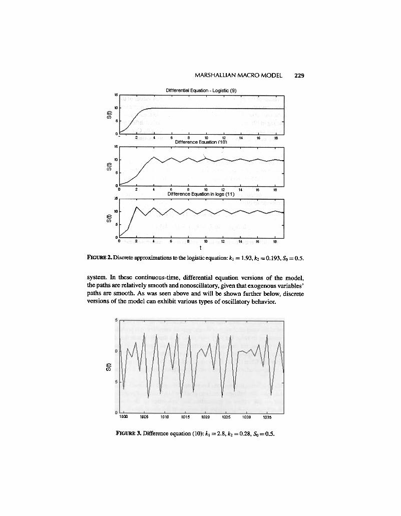
While the differential equation in (9) with constant parameters exhibits a smoothconvergence to its limiting value, the processes in (10) and (11) can exhibitoscillatory behavior. Further, in computed examples, the paths associated with(10) and (11) differed considerably in many cases. For example, it was found thatthe equations in (10) and (11) gave rise to a smooth approach to an equilibriumvalue when 0 < k1 < 1 and k2 > 0 and oscillatory approaches to equilibrium whenk1 > 1. See plots of solutions to (9), (10), and (11) in Figures 2 and 3 for differentvalues of the parameter k1. Note that (10) and (11) can yield quite differentsolutions for the same value of the parameter. Also, if the measured values ofS have additive or multiplicative biases, the properties of (10) and (11) will befurther affected. Last, note that since the coefficients of (9), (10), and (11) arefunctions of the rates of change of the exogenous variables, it is probable that theyare not constant in value but vary with time. It is thus fortunate that data can bebrought to bear on, for example, discrete versions of equation (8) that allow forvariation in the exogenous variables; see, for example, Veloce and Zellner (1985)and Zellner and Chen (2001) for examples of such fitted functions. Also, discreteversions of the structural equation system presented above can be estimated usingdata.

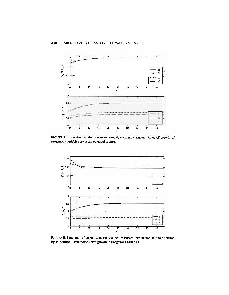
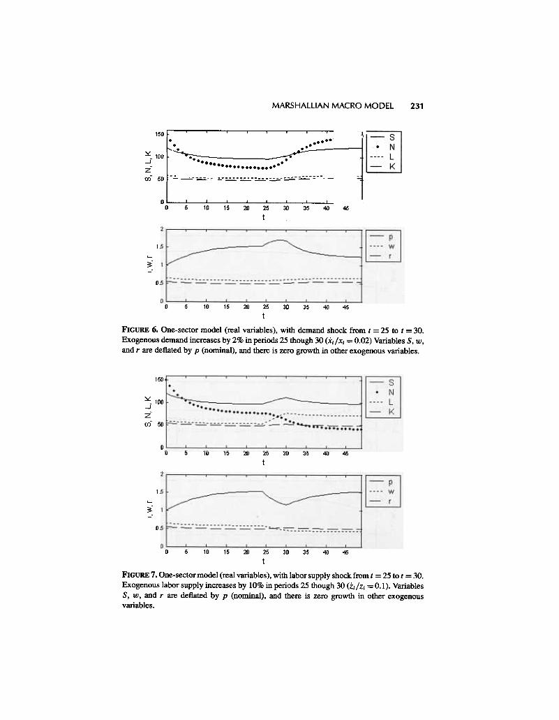
Various simulation experiments have been done with the seven-equation modeldescribed above that indicate that it can produce a rich range of possible solutions,depending on the values of parameters and properties of input variables. Forexample, in Figures 4-7 are shown the outputs of the seven-equation model undervarious conditions. In Figures 4 and 5, the paths of the nominal and real vari-ables are shown when the model is started up at nonequilibrium initial values.Figures 6 and 7 show how shocks to demand and to factor supplies affect the


~00

t

FIGURE 2. Discrete approximations to the logistic equation: k1 = 1.93, k2 = 0.193, So = 0.5.

system. In these continuous-time, differential equation versions of the model,the paths are relatively smooth and nonoscillatory, given that exogenous variables'paths are smooth. As was seen above and will be shown further below, discreteversions of the model can exhibit various types of oscillatory behavior.

8CJ)

1000 IDD5 1010 1015 1020 1025 1030 1035

FIGURE 3. Difference equation (10): k1 = 2.8, k2 = 0.28, So = 0.5.


15D~

~ 100-J-Z

00- 50

-.. j. ..."--':';;':"

~-:..:.=-- ~- ~ -~ -:.:..:;.- ==.- ==.- ==.- ==.- ==.-

II' , ., , , , , , , ,0 5 10 15 20 25 30 35 40 46

f2

1.b~

~ 1Co

0.5

~

,-:' ::.::. ' :.:.:. -::.:.:. -::.:.:. -:.::. -:.::..:. -:.::. -:.::. -:.::. -:.::. -:.::. -:.::. -

U' , ., , , , , , , ,0 5 10 15 20 25 30 35 ~ 45

t

FIGURE 4. Simulation of the one-sector model, nominal variables. Rates of growth ofexogenous variables are assumed equal to zero.

150.

~ 100 '

ICO 50

...,~-:-=.;;.-:~:~:~=-~-~-=_.:-. :::~::~:..~.~

---L-K

0 ' , ., , , , , , ,0 5 10 15 20 25 30 35 40 45

t

0 5 10 15 20 25 30 35 40 45

t

FIGURE 5. Simulation of the one-sector model, real variables. Variables S, W, and r deflatedby p (nominal), and there is zero growth in exogenous variables.


.,'..,. '..;...~.........~~~'::---~ ;~,:.--..'0 =-=- -;- =:.,- =. -=. -~-:;=.;. -~ -:.:.:. -='" -

150.

~ 100Jz(/)- 50 ,---~--.

0 I I I , ., , , , , I0 5 10 15 20 25 30 35 40 45

t

2

-.,~

1.!J ! ""

~

~

~-

.,.-/

~ -~ -:.::. -:.:.:. -:=..:. -:=..:. -:.:.:. -:..:;. -:.:.:. -:.::. -:.::. -:.::. -0.0 I

0 ' , ., , , , , , ,0 5 10 15 20 25 30 35 40 46

t

FIGURE 6. One-sector model (real variables), with demand shock from t = 25 to t = 30.Exogenous demand increases by 2% in periods 25 though 30 (x; Ix; = 0.02) Variables S, W,and r are deflated by p (nominal), and there is zero growth in other exogenous variables.

15D~.--.!..~ 100

Jz00- 50

0 ' , , , , ., , , , ,0 5 10 15 20 25 30 35 40 46

t

2

1.b I "'-/ 1

-----

~

~- .,

I0.0 I ~-~,~_:":"::"-:":""="_:":"::"_:":"::"_:;

o. , ., , .0 5 10 15 20 25 30 35 40 46

t

FIGURE 7. One-sector model (real variables), with labor supply shock from t = 25 to t = 30.Exogenous labor supply increases by 10% in periods 25 though 30 (Zi/Zi = 0.1). VariablesS, w, and r are deflated by p (nominal), and there is zero growth in other exogenousvariables.

ARNOLD ZELLNER AND GUILLERMO ISRAILEVICH232

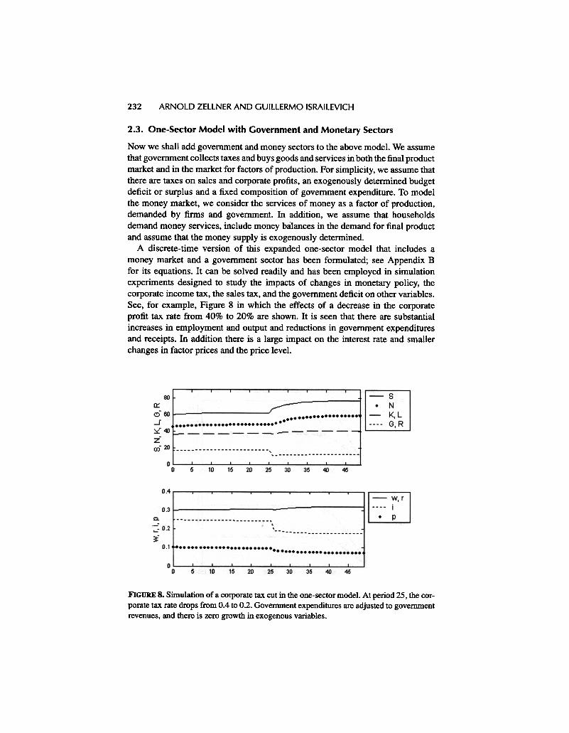
2.3. One-Sector Model with Government and Monetary Sectors

Now we shall add government and money sectors to the above model. We assumethat government collects taxes and buys goods and services in both the final productmarket and in the market for factors of production. For simplicity, we assume thatthere are taxes on sales and corporate profits, an exogenously determined budgetdeficit or surplus and a fixed composition of government expenditure. To modelthe money market, we consider the services of money as a factor of production,demanded by firms and government. In addition, we assume that householdsdemand money services, include money ba:tances in the demand for final productand assume that the money supply is exogenously determined.

A discrete-time version of this expanded one-sector model that includes amoney market and a government sector has been formulated; see Appendix Bfor its equations. It can be solved readily and has been employed in simulationexperiments designed to study the impacts of changes in monetary policy, thecorporate income tax, the sales tax, and the government deficit on other variables.See, for example, Figure 8 in which the effects of a decrease in the corporateprofit tax rate from 40% to 20% are shown. It is seen that there are substantialincreases in employment and output and reductions in government expendituresand receipts. In addition there is a large impact on the interest rate and smallerchanges in factor prices and the price level.

FIGURE 8. Simulation of a corporate tax cut in the one-sector model. At period 25, the cor-porate tax rate drops from 0.4 to 0.2. Government expenditures are adjusted to governmentrevenues, and there is zero growth in exogenous variables.


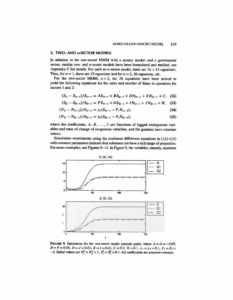
3. TWO- AND n-SECTOR MODELS

In addition to the one-sector MMM with a money market and a governmentsector, similar two- and n-sector models have been formulated and studied; seeAppendix C for details. For such an n-sector model, there are 7n + 12 equations.Thus, for n = 1, there are 19 equations and for n = 2,26 equations, etc.

For the two-sector MMM, n = 2, the 26 equations have been solved toyield the following equations for the sales and number of firnls in operation forsectors 1 and 2:

'.(SIt -Slt-I)/Slt-1 = AS1t-1 + BS2t-1 + DN1t-l + EN2t-1 + C, (12)

(S2t -S2t-I)/S2t-1 = FSlt-1 + GS2t-1 + IN1t-1 + JN2t-1 + H, (13)

(Nlt -N1t-I)/ Nlt-l = Yl (Slt-l -F1Nlt-l), (14)

(N2t -N2t-l)/ N2t-1 = Y2(S2t-1 -F2N2t-I), (15)

where the coefficients, A, B, ..., J are functions of lagged endogenous vari-ables and rates of change of exogenous variables, and the gammas have constantvalues.

Simulation experiments using the nonlinear difference equations in (12)-(15)with constant parameters indicate that solutions can have a rich range of properties.For some examples, see Figures 9-13. In Figure 9, the variables, namely, numbers

8, 81, 82

30 I

/20 I

0

10 I

J /==" -:;,Y'~ -../ .

--70

0 50 100 150

t

FIGURE 9. Simulation for the two-sector model (smooth path), where A = G = -0.07,B=F=0.05, D= 1=0.01, E=l =0.01, C=0.2, H=O.l, Yl =Y2=0.1, Fl =F2=-2. Initial values are NP = N~ = 1, sr = ~ = 0.1. All coefficients are assumed constant.

234

ARNOLD

ZELLNER AND GUILLERMO ISRAILEVICH

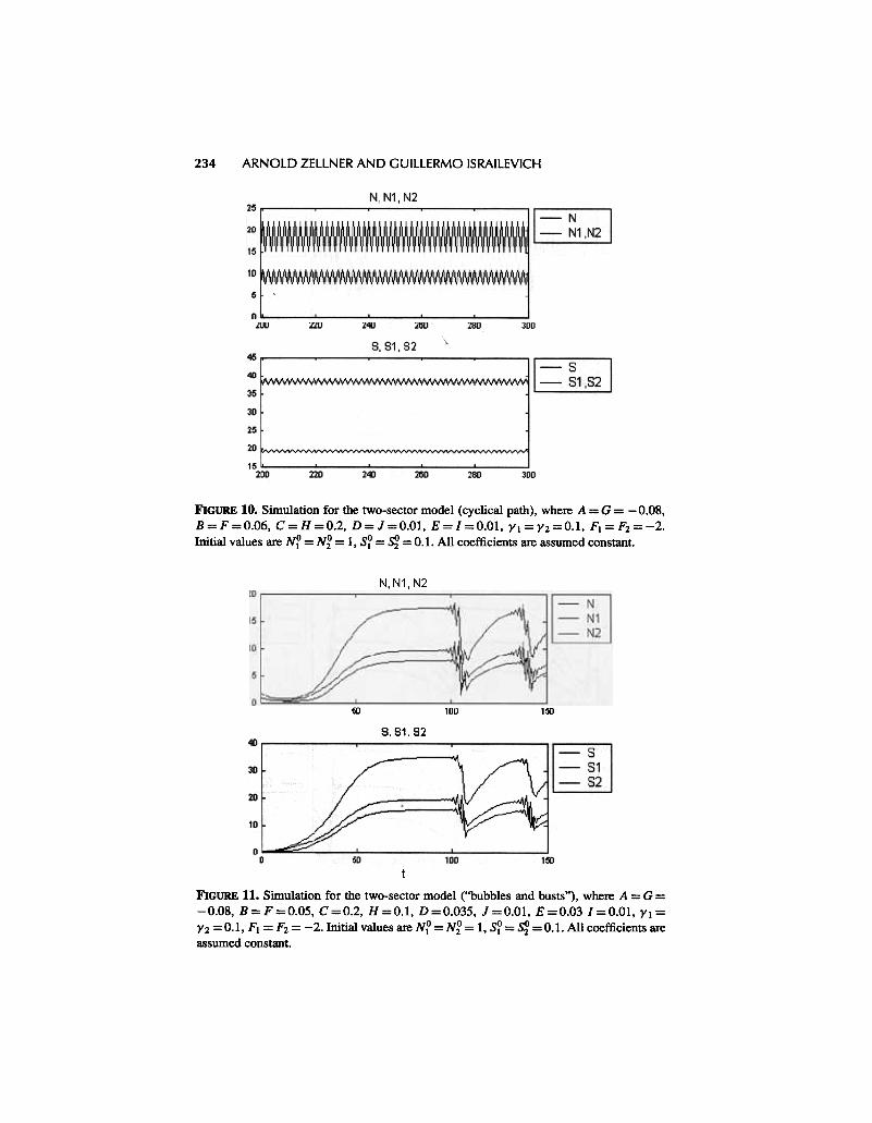
FIGURE 10. Simulation for the two-sector model (cyclical path), where A = G = -0.08,B=F=0.06, C=H=0.2, D=J=O.Ol, E=/=O.Ol, Yl=Y2=0.1, F1=F2=-2.Initial values are NP = Nf = 1, s? = ~ = 0.1. All coefficients are assumed constant.

N,N1, N2

60 100 IW

8, 81, 82

t

FIGURE 11. Simulation for the two-sector model ("bubbles and busts"), where A = G =

-0.08, B=F=0.05, C=0.2, H=O.I, D=0.035, J=O.OI, E=0.03 1=0.01, Yl=Y2 =0.1, Fl = F2 = -2. Initial values are Nr = Nf = 1, s? = sf] =0.1. All coefficients are

assumed constant.


N,N1,N2 I-N I25~,," ' '.., " " '.:,' J'=~i!

20 , , .

0 I, , , ., ., , , , I

1000 1010 1020 1030 10~ 10~0 1060 1070 1080 1090 1100

8,81,82

401

~w.ANwvVlNW"'N\N'.Nv"""""""'~~

30 I

:~~:::~::::======::==::~~~j20 I

10 I

0 " , , , , , , , , , ,1000 1010 1020 1030 1040 10~0 1050 1010 1080 1090 1100

t

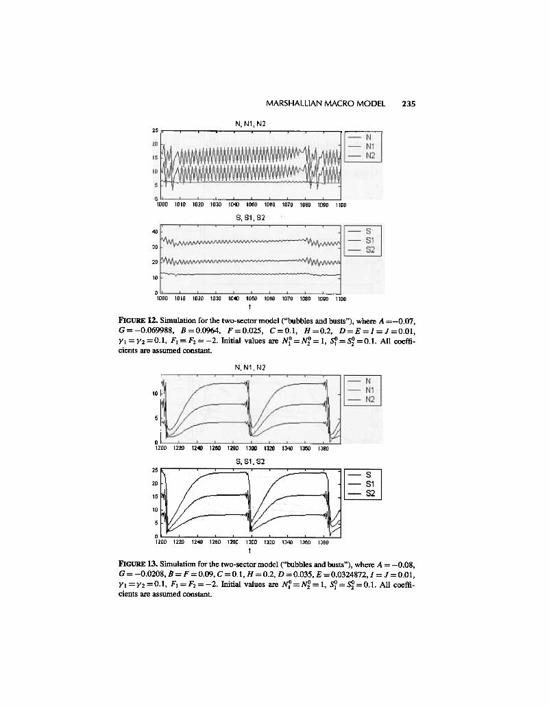
FIGURE 12. Simulation for the two-sector model ("bubbles and busts"), where A =-0.07,G=-0.069988, B=0.0964, F=0.025, C=O.I, H=0.2, D=E=I=J=O.OI,Yl=Y2=0.1, F1=F2=-2.lnitial values are NP=Nf=l, SP=Sf=O.I. All coeffi-cients are assumed constant.

N, N1, N2

-N

-N1-N2

/,

~10 I

:~i~=--~.

.:t11200 1220 1241 1200 1280 1300 1320 1340 1300 1380

8, 81, 82

/-~-~I

-"'/'

1200 1220 12~ 1200 1280 1300 1320 13~ 1300 1380

1

FIGURE 13. Simulation for the two-sector model ("bubbles and busts"), where A = -0.08,G= -0.0208, B=F=O.09,C=O.I, H=0.2, D=0.035, E=0.0324872, 1= 1=0.01,Yl=Y2=0.1, F1=F2=-2. Initial values are NP=Nf=l, S?=Sf=O.I. All coeffi-cients are assumed constant.


of finDS in operation in the two-sectors and sales of the two-sectors follow rathersmooth paths to their equilibrium values. However, with the parameter values usedfor the experiments described in Figure 10, the paths of the variables in the twosectors show systematic, recurrent, cyclical properties. In contrast to the relativelysmooth and systematic features shown in Figures 9 and 10, with the parametervalues employed in experiments reported in Figures 11-13, it is seen that varioustypes of "bubbles and busts" behavior are exhibited by the two-sector MMM. Itis thus apparent that this relatively simple model has a broad range of possiblesolutions, even when the rates of change o( the exogenous variables are assumedto have constant values. Allowing for changes in the exogenous variables' growthrates of course enlarges the range of possible solutions to this two-sector modeland MMMs containing more than two sectors.

4. SUMMARY AND CONCLUSIONS

In this report, we have briefly reported our progress in producing one-, two- and n-sector versions of the MMM that are rooted in traditional economic theory and yetprovide a rich range of possible forms that can be implemented with sector data.For example, Zellner and Chen (2001) implemented the MMM's reduced-formequations in forecasting 11 U.S. industrial sectors' annual outputs and their totalusing various estimation and forecasting techniques with encouraging results, asmentioned in Section 1. These results indicate that it pays to disaggregate to obtainimproved forecasts of aggregate, real GDP growth rates as well as sector forecasts.Of course, such results may be improved by using the structural equations forsectors rather than just one reduced-form equation per sector.

Further, there are many ways to improve the "bare bones" MMMs that wepresented above by drawing on the vast economic literature dealing with entryand exit behavior, anticipations, various industrial structures, alternative forms ofproduction and demand relations, dynamic optimization procedures, introductionof stochastic elements, etc. In addition, there is a need to consider inventoryinvestment, intermediate goods, vintage effects on capital formation, imports andexports, etc. Although the list of extensions is long, just as in the case of theModel T Ford, we believe that our MMM is a fruitful initial model that willbe developed further to yield improved, future models in the spirit of Deming'semphasis on continuous improvement. Most satisfying to us is the fact that we havean operational, rich, dynamic "core" model that is rationalized by basic economictheory. This case of "theory with measurement" is, in our opinion, much to bepreferred to "measurement without theory" or "theory without measurement."

REFERENCES

Cunningham, W.J. (1958) Introduction to Nonlinear Analysis. New York: McGraw-Hill.Brock, W.A. & A.G. Malliaris (1989) Differential Equations, Stability and Chaos in Dynamic Eco-

nomics. Amsterdam: North-Holland.Day, R.H. (1982) Irregular growth cycles. American Economic Review 72, 406-414.


Day, R.H. (1994) Complex Economic Dynamics, Vol. 1: An Introduction to Dynamical Systems andMarket Mechanisms. Cambridge, MA: MIT Press.

de Alba, E. & A. Zellner (1991) Aggregation, Disaggregation, Predictive Precision and Modeling.

Manuscript, H.G.B. Alexander Research Foundation.Hong, C. (1989) Forecasting Real Output Growth Rates and Cyclical Properties of Models: A Bayesian

Approach. PhD. Dissertation, University of Chicago.Kahn, P.B. (1989) Mathematical Methodsfor Scientists and Engineers: Unear and Nonlinear Systems,

New York: Wiley.Koop, G., M.H. Peasaran & S.M. Potter (1996) Impulse response analysis in nonlinear multivariate

models. Journal of Econometrics 74, 119-148.Liitkepohl, H. (1986) Comparisons of predictors for temporally and contemporaneously aggregated

time series. International Journal of Forecasting 2, 461-475.Min, C. (1992) Economic Analysis and Forecasting of International Growth Rates Using Bayesian

Techniques. Pill. Dissertation, University of Chicago.Palm, F.C. (1976) Testing the dynamic specification of an econometric model with an application to

Belgian data. European Economic Review 8, 269-289.Palm, F.C. (1977) On univariate time series methods and simultaneous equation econometric models.

Journal of Econometrics 5, 379-388.Palm, F.C. (1983) Structural econometric modeling and time series analysis: An integrated approach.

In A. Zellner (ed.), Applied Time Series Analysis of Economic Data, pp. 199-223. Washington, DC:Bureau of the Census, U.S. Department of Commerce.

Quintana, I.M., B.H. Putnam & D.S. Wilford (1997) Mutual and pension fund management: Beatingthe markets using a global Bayesian investment strategy. Annual Proceedings Volume, Section onBayesian Statistical Science. American Statistical Association.

Veloce, W. & A. Zellner (1985) Entry and empirical demand and supply analysis for competitiveindustries. Journal of Econometrics 30, 459-471.

Zamowitz, V. (1986) The record and improvability of economic forecasting. Economic Forecasting 3,22-31.

Zellner, A. (1962) On the Questionable Virtue of Aggregation. Workshop paper 6202, Social SystemsResearch Institute, University of Wisconsin [published in Zellner (2004 Appendix)].

Zellner, A. (1997) Bayesian Analysis in Econometrics and Statistics. Cheltenham: Edward Elgar.Zellner, A. (2000) Bayesian and non-Bayesian approaches to scientific modelling and inference in

economics and econometrics. Korean Journal of Money & Finance 5(2),11-56.Zellner, A. (2001) The Marshallian macroeconomic model. In T. Nagishi, R.V. Ramachandran &

K. Mino (eds.), Economic Theory, Dynamics and Markets: Essays in Honor of Ryuzo Sato,pp. 19-29. Dordrecht: Kluwer.

Zellner, A. (2004) Statistics, Econometrics and Forecasting. Cambridge, UK: Cambridge UniversityPress.

Zellner, A. & B. Chen (2001) Bayesian modeling of economies and data requirements. Macroecono-mic Dynamics 5, 673-700.

Zellner, A. & C. Min (1999) Forecasting turning points in countries' growth rates: A response toMilton Friedman. Journal of Econometrics 40, 183-202.

Zellner, A. & F.C. Palm (1974) Time series analysis and simultaneous equation econometric models.Journal of Econometrics 2, 17-54 [reprinted in Zellner and Palm (2004)].

Zellner, A. & F.C. Palm (1975) Time series analysis of structural monetary models of the U.S. economy,Sankya, Ser. C, 37, 12-56 [reprinted in Zellner and Palm (2004)].

Zellner, A. & F.C. Palm (2004) The Structural Econometric Modeling, Time Series Analysis (SEMTSA)

Approach. Cambridge, UK: Cambridge University Press.Zellner, A. & I. Tobias (2000) A note on aggregation, disaggregation and forecasting Journal of

Forecasting 19,457-469.Zellner, A., C. Hong & C. Min (1991) Forecasting turning points in international output growth rates

using Bayesian exponentially weighted autoregression, time varying parameter and pooling tech-niques. Journal of Econometrics 49, 275-304.


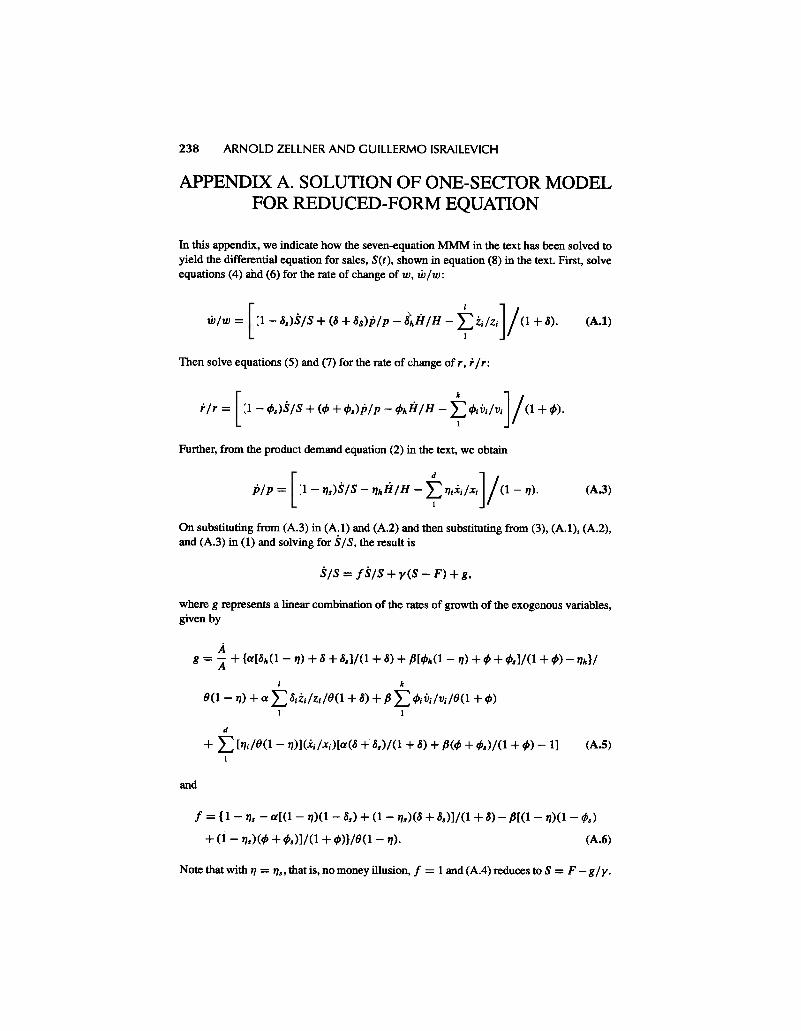
APPENDIX A. SOLUTION OF ONE-SECTOR MODELFOR REDUCED-FORM EQUATION

In this appendix, we indicate how the seven-equation MMM in the text has been solved toyield the differential equation for sales, 8(t), shown in equation (8) in the text. First, solveequations (4) and (6) for the rate of change of w, liJ/w:

w/w = (A.I)(1 -8.)S/S + (8 + 8s)jJ/p -t/oH/H -~Zi/Zi]1 (1 + 8).

Then solve equations (5) and (7) for the rate of change of r. r / r:

fir = (1 -I/>.)S/S + (I/> + I/>.)p/ p -I/>hH / H -~ l/>iVi/Vi ] 1(1 + 1/».

Further, from the product demand equation (2) in the text, we obtain

(A.3)pip = (1 -'1,)S/S -'1hiI/H -~ '1iXi/Xi] I (1 -'1).

On substituting from (A.3) in (A.I) and (A.2) and then substituting from (3), (A. 1), (A.2),and (A.3) in (1) and solving for S/S, the result is

SIS = ISIS + y(S -F) + g,

where g represents a linear combination of the rates of growth of the exogenous variables,given by

Ag = A + {a[b'h(1 -'1) + b' + b'.]/(1 + b') + fJ[4>h(1 -'1) + 4> + 4>.]/(1 + 4» -'1h}/

I k

9(1 -II) + a L 8izi/zi/9(1 + 8) +.8 L 4>ivi/vi/9(1 + 4»1 1

d

+ L ['1i/(J(1 -'1)] (Xi/Xi)[a(8 0+: 8,)/(1 + 8) + /3(4> + 4>,)/(1 + 4» -1]1

(A.5)

and

f = {I -'1. -a[(1 -'1)(1 -8.) + (1 -'1.)(8 + 8.)]/(1 + 8) -,8[(1 -'1)(1 -1/>.)

+ (1 -'1.)(t!> + 1/>.)]/(1 + t!»}/8(1 -'1). (A.6)

Note that with 17 = 17., that is, no money illusion, f = 1 and (Ao4) reduces to S = F -glyo


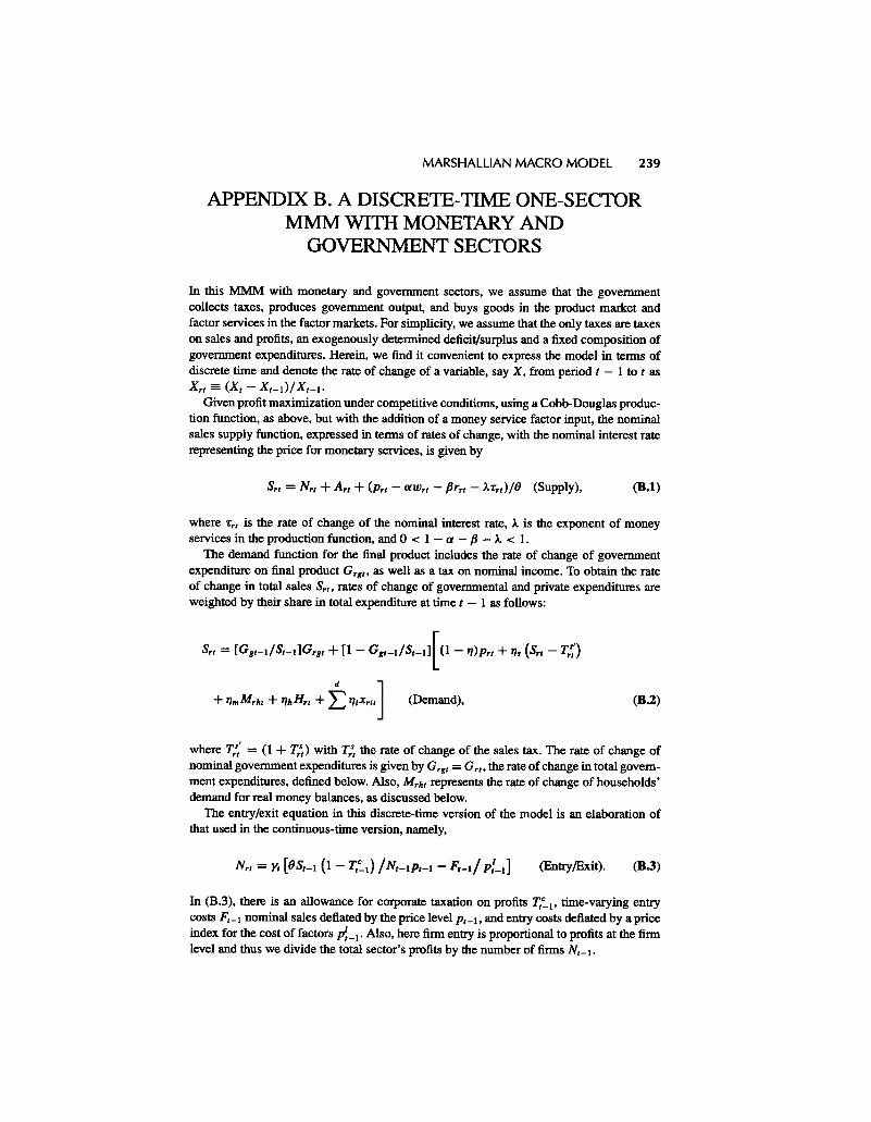
APPENDIX B. A DISCRETE- nME ONE-SECTORMMM WITH MONETARY AND

GOVERNMENT SECTORS

In this MMM with monetary and government sectors, we assume that the governmentcollects taxes, produces government output, and buys goods in the product market andfactor services in the factor markets. For simplicity, we assume that the only taxes are taxeson sales and profits, an exogenously detennined deficit/surplus and a fixed composition ofgovernment expenditures. Herein, we find it convenient to express the model in terms ofdiscrete time and denote the rate of change of a variable, say X, from period t -I to t asXrt = (Xt -Xt-l)/Xt-l'

Given profit maximization under competitive conditions, using a Cobb-Douglas produc-tion function, as above, but with the addition of a money service factor input, the nominalsales supply function, expressed in terms of rates of change, with the nominal interest raterepresenting the price for monetary services, is given by

(B.I)S" = N" + A" + (p" -aw" -.8r" -At',,)/lJ (Supply),

where 'Crl is the rate of change of the nominal interest rate, A is the exponent of moneyservices in the production function, and 0 < 1 -a -.8 -A < 1.

The demand function for the final product includes the rate of change of governmentexpenditure on final product Grgl, as well as a tax on nominal income. To obtain the rateof change in total sales SrI. rates of change of governmental and private expenditures areweighted by their share in total expenditure at time t -1 as follows:

SrI = [Ggt-I/St-JGrgt + [1 -Ggt-I/St-l] [ (1 -FI)Prt + Fl. (Srt -T::)

d

+ 1/mMrht + 1/hHrt + L 1/iXrit (Demand), (B.2)

where r:: = (1 + r:t) with r:t the rate of change of the sales tax. The rate of change ofnominal government expenditures is given by Grgt = Grt, the rate of change in total govern-ment expenditures, defined below. Also, Mrht represents the rate of change of households'demand for real money balances, as discussed below.

The entry/exit equation in this discrete-time version of the model is an elaboration ofthat used in the continuous-time version, namely,

NTt = Yt [8St-l (1- 7;~I) /Nt-1Pt-l -Ft-l/p{-l] (Entry/Exit). (B.3)

In (B.3), there is an allowance for corporate taxation on profits ~~l' time-varying entrycosts Ft-l nominal sales deflated by the price level Pt-l, and entry costs deflated by a priceindex for the cost of factors P:-l. Also, here finn entry is proportional to profits at the finnlevel and thus we divide the total sector's profits by the number of finns Nt-l.


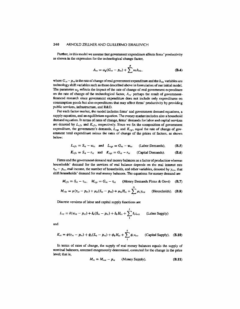
Further, in this model we assume that government expenditure affects fi11Ils' productivityas shown in the expression for the technological change factor,

B

Art = (J)g(Grt -Prt) + L (J)ibrit. (B.4)

where Grt- Prt,is the rate of change of real government expenditure and thebrit variables aretechnology shift variables such as those described above in fonnulation of our initial model.The parameter Wg reflects the impact of the rate of change of real government expenditureon the rate of change of the technological factor, Art' perhaps the result of government-financed research since government expenditure does not include only expenditures onconsumption goods but also expenditures that may affect finns' productivity by providingpublic services, infrastructure, and R&D.

For each factor market, the model includes finns' and government demand equations, asupply equation, and an equilibrium equation. The money market includes also a householddemand equation. In tenns of rates of change, finns' demands for labor and capital servicesare denoted by Lrft and Krft, respectively. Since we fix the composition of governmentexpenditure, the government's demands, Lrgt and Krgt, equal the rate of change of gov-ernment total expenditure minus the rates of change of the prices of factors, as shownbelow:

(Labor Demands),

(Capital Demands).

(D.5)

(D.6)

Lrft = SrI -Wrt and Lrgt = Grt -Wrt

Krft = SrI -rrt and Krgt = Grt -rrt

Firms and the government demand real money balances as a factor of production whereashouseholds' demand for the services of real balance depends on the real interest rate'Crt -Prt, real income, the number of households, and other variables, denoted by Yrit, thatshift households' demand for real money balances. The equations for money demand are

Mrfl = SrI -1"rlo Mrgl = Grl -1"rl (Money Demands Finns & Govt) (B.7)

m

Mrhl = 11-(1"rl -Prl) + 11-. (SrI -Prl) + I1-hHrl + L l1-iYril (Households). (B.S)

Discrete versions of labor and capital supply functions are

I

Lrt = ,s(wrt -Prt) + ,s..(Srt -Prt) + ,sJlHrt + L ,siZrit1

(Labor Supply)

and

k

Krt = tfJ(rrt -Prt) + tfJ,(Srt -Prt) + tfJhHrt + L tfJiVrit

1(Capital Supply). (B.IO)

In terms of rates of change, the supply of real money balances equals the supply ofnominal balances, assumed exogenously determined, corrected for the change in the pricelevel; that is,

Mrt = Mrot -Prt (Money Supply). (B.II)


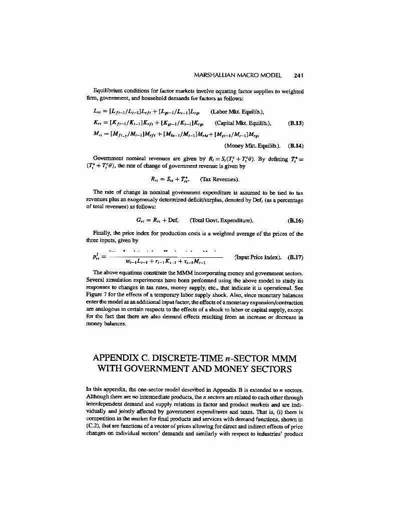
Equilibrium conditions for factor markets involve equating factor supplies to weightedfirm, government, and household demands for factors as follows:

Lrt = [Llt-IILt-uLrlt + [Lgt-lILt-l]Lrgt (Labor Mkt Equilib.),

Krt = [KIt-II Kt-l] Krlt + [Kgt-l1 Kt-l]Krgt (Capital Mkt Equilib.),

Mrt = [M It_!1 Mt-l]Mrlt + [Mht-l1 Mt-l]Mrht+ [Mgt-l1 Mt-l]Mrgt

(Money Mkt. Equilib.).

(B.13)

(B.14)

Government nominal revenues are given by R, = S,(T,S + T,C(). By defining T,* =(T,s + T,C(), the rate of change of government revenue is given by

Rrt = SrI + Tr;. (Tax Revenues).

The rate of change in nominal government expenditure is assumed to be tied to taxrevenues plus an exogenously deten1lined deficit/surplus, denoted by Deft (as a percentageof total revenues) as follows:

Grt = Rrt + Deft (B.16)(Total Govt. Expenditure).

Finally, the price index for production costs is a weighted average of the prices of thethree inputs, given by

(Wt-ILt-l)Wrt + (rt-lKt-l)rrt + (rt-lMt-l)rrt1 -Pt- ,r Wt-ILt-l + Tt-1Kt-l + Tt-1Mt-l

The above equations constitute the MMM incorporating money and government sectors.Several simulation experiments have been performed using the above model to study itsresponses to changes in tax rates, money supply, etc., that indicate it is operational. SeeFigure 7 for the effects of a temporary labor supply shock. Also, since monetary balancesenter the model as an additional input factor, the effects of a monetary expansion/contractionare analogous in certain respects to the effects of a shock to labor or capital supply, exceptfor the fact that there are also demand effects resulting from an increase or decrease inmoney balances.

{Input Price Index). (B.17)

APPENDIX C. DISCRETE- llME n-SECTOR MMMWITH GOVERNMENT AND MONEY SECTORS

In this appendix, the one-sector model described in Appendix B is extended to n sectors.Although there are no intermediate products, the n sectors are related to each other throughinterdependent demand and supply relations in factor and product markets and are indi-vidually and jointly affected by government expenditures and taxes. That is, (i) there iscompetition in the market for final products and services with demand functions, shown in(Co2), that are functions of a vector of prices allowing for direct and indirect effects of pricechanges on individual sectors' demands and similarly with respect to industries' product


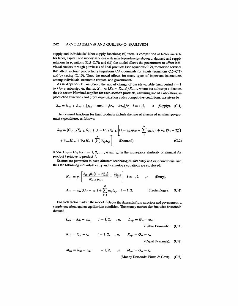
supply and individuals' labor supply functions; (ii) there is competition in factor marketsfor labor, capital, and money services with interdependencies shown in demand and supplyrelations in equations (C.5-C.7); and (ill) the model allows the government to affect indi-vidual sectors through purchases of final products (see equations C.2), to provide servicesthat affect sectors' productivity (equations C.4), demands for inputs (equations C.5-C.7)and by taxing (C.15). Thus, the model allows for many types of important interactionsamong individuals, economic entities, and government.

As in Appendix B, we denote the rate of change of the ith variable from period t -Ito t by a subscript rit, that is, Xril = [XiI -Xil-I]/ XiI-I, where the subscript i denotesthe ith sector. Nominal supplies for each sector's products, assuming use of Cobb-Douglasproduction functions and profit maximization under competitive conditions, are given by

Srit = Nrit + Arit + [Prit -aWrt -.8rrt -A't'rt]/9i i = 1,2, n (Supply). (C.t)

The demand functions for final products include the rate of change of nominal govern-ment expenditure, as follows:

Sril = [Gil-I/SiI-l]Gril + [1 -GiI/SiI-l] [(1 -'1ii)Pril + ~ '1ijPrjl + III;, (SrI -T::)d ~

+ lIIimMrhl + lIIihHrl + L lIIijxrjl (Demand), (C.2)

where Grit = Grt for i = 1, 2, ..., n and 7/ij is the cross-price elasticity of demand forproduct i relative to product j.

Sectors are permitted to have different technologies and entry and exit conditions, andthus the following individual entry and technology equations are employed:

i = 1,2, (Entry),,n

BArit = W;g(Grt -Prt) + }=:wijbrjt i = 1,2,

j=l(CA)(Technology).

For each factor market, the model includes the demands from n sectors and government, asupply equation, and an equilibrium condition. The money market also includes householddemand.

i = 1,2,Lrit = Srit -Wrt. ,n, Lrg, = Gr, -Wrt

(Labor Demands), (C.5)

i = 1,2,Krit = Srit -rrt, ,n, Krgt = Grt -rrt

(Capal Demands), (C.6)

= 1,2,Mrit = Srit -1'rt. ,n Mrgt = Grt -'rrt

(Money Demands: Finns & Govt), (C.7)

MARSHALLIAN MACRO MODEL

m

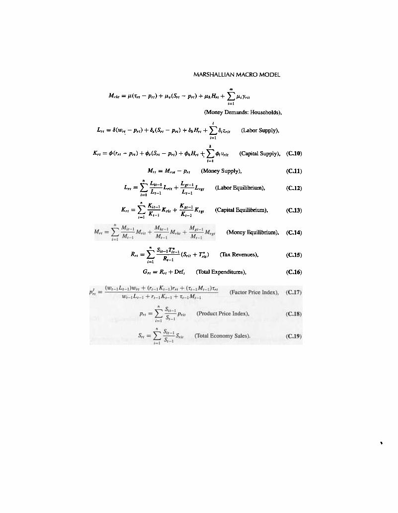
Mrht = JL(t'rt -Prt) + JL.(Srt -Prt) + JLhHrt + L JLiYrit;=1

(Money Demands: Households),

I

Lrt = B(wrt. -Prt) + B.(Srt -Prt) + BhHrt + L BiZrit (Labor Supply).i=1

k

Krt = 4>(rrt -Prt) + 4>. (Srt -Prt) + 4>hHrt -+: L 4>ivriti=1

Mrt = Mrot -Prt (Money Supply).

(Capital Supply), (C.I0)

(C.II)

(Labor Equilibrium), (C.I2)~ Lil-1 LgI-ILrl = L., -L Lril + ~Lrgli=1 I-I I-I

~ Kil-1 KgI-IKrl = L., ~ Kril + -x:-- Krgli=1 I-I I-I

(Capital Equilibrium), (C.13)

(Money Equilibrium), (C.14)

L" Sit-I~~-I(S ' + T~)R -Tit Tit Tt -

Rt-1i=1(C.tS)(Tax Revenues),

Grt = Rrt + Deft (Total Expenditures), (C.16)

,

Documents

MD SURVEY MARSHALLIAN MACROECONOMIC MODEL: A …