Embed Size (px)
Citation preview
BEST-REPLY SEARCH IN MULTI-PLAYERCHESS
Markus Esser
Master Thesis 12-13
Thesis submitted in partial fulfilmentof the requirements for the degree of
Master of Science of Artificial Intelligenceat the Faculty of Humanities and Sciences
of Maastricht University
Thesis committee:
Dr. M.H.M. WinandsDr. M.P.D. Schadd
Dr. ir. J.W.H.M UiterwijkJ.A.M Nijssen, M.Sc.
Maastricht UniversityDepartment of Knowledge Engineering
Maastricht, The NetherlandsJuly 2012

Preface
This report is my master thesis. It describes the performed research at the Department of KnowledgeEngineering at Maastricht University. In this thesis, four variants of the multi-player search algorithmbest-reply search are proposed. These proposed algorithms are tested in the domain of multi-player Chess.I would like to thank both my supervisors dr. Maarten Schadd and dr. Mark Winands. Dr. MaartenSchadd was my supervisor during the first part of the thesis and gave me practical hints for the imple-mentation of the existing algorithms and search enhancements. Especially, he indicated common sourcesof errors which probably reduced the time for debugging the algorithms. During the last part of thethesis, dr. Mark Winands was my daily supervisor. His knowledge about programming Artificial Intel-ligence in Chess was helpful to increase the performance of my program for playing multi-player Chess.Additionally, his input and corrections were useful to improve this report. I also would like to thankmy fellow student Michael Gras for a lot of interesting discussions about the proposed best-reply variantsand how they perform in different domains. Finally, I would like to thank my parents who supported meduring this thesis and the whole studies.I got the idea to propose variants of the best-reply search during the course “Intelligent Search Techniques”given as part of the Master of Artificial Intelligence at the Department of Knowledge Engineering. Thebest-reply search, recently invented at this Department, was mentioned in this course as a promisingsearch algorithm for multi-player games.
Markus EsserMaastricht, July 2012

Abstract
Computers have been used to play board games, especially Chess, since their earliest days. Researchersmainly concentrated on building strong programs for playing two-player games. Therefore much researchcan still be done in the area of multi-player games. This thesis is about search algorithms in multi-playergames. A program for playing multi-player Chess is build as a test domain to perform research on it.Multi-player Chess is a Chess variant for four players. As regular Chess, multi-player Chess is a capturegame with perfect information. Although Monte-Carlo Tree Search nowadays has become popular in thearea of games, this thesis focusses on evaluation function based search. Recently, a new promising searchalgorithm for multi-player games, called best-reply search, was proposed by Schadd and Winands (2011).In this algorithm, only the opponent with the strongest counter-move is allowed to play a move. The otheropponents pass their turn. Although best-reply performs well in the games tested so far, it has conceptualdrawbacks. The main drawback of best-reply search is that the search can lead to officially unreachableand sometimes illegal board positions. The concern of this thesis is to overcome these drawbacks andthus, to improve the performance of best-reply search. Therefore the problem statement is:How can the best-reply search be modified to outperform the paranoid algorithm in complex (capturing)multi-player games?To introduce the test domain in which the research is performed, this thesis starts with an explanation ofthe rules of multi-player Chess. Afterwards, the existing search algorithms and their enhancements aredescribed. Next, new search algorithms based on the best-reply search are proposed. These algorithms areexplained and analyzed. The main idea to overcome the drawbacks of best-reply is to let the opponentsplay the best move regarding the static move ordering instead of passing as done in best-reply search.After a description of the evaluation function, which is required to gain reasonable play in the area ofmulti-player Chess, the proposed algorithms are tested against the existing ones. The experiments showthat one of the proposed algorithms, namely BRS1,C−1, is able to outperform the existing algorithmsin the domain of multi-player Chess. In BRS1,C−1, the opponent with the strongest counter-move isallowed to perform a search while the other opponents play the best move regarding the static moveordering. Because of the strong performance in multi-player Chess, BRS1,C−1 is a promising searchalgorithm. Further tests have to be performed to detect whether it also works well in other domains thanmulti-player Chess.

Contents
Preface iii
Abstract v
Contents vii
List of Figures 1
List of Tables 3
List of Algorithms 5
1 Introduction 71.1 Games and Artificial Intelligence (AI) . . . . . . . . . . . . . . . . . . . . . . . . . . . . . 71.2 AI in Multi-Player Games . . . . . . . . . . . . . . . . . . . . . . . . . . . . . . . . . . . . 7
1.2.1 Evaluation Function Based Search . . . . . . . . . . . . . . . . . . . . . . . . . . . 81.2.2 Monte-Carlo Tree Search (MCTS) . . . . . . . . . . . . . . . . . . . . . . . . . . . 8
1.3 Problem Statement and Research Questions . . . . . . . . . . . . . . . . . . . . . . . . . . 91.4 Outline of the Thesis . . . . . . . . . . . . . . . . . . . . . . . . . . . . . . . . . . . . . . . 10
2 Multi-Player Chess 112.1 Two-Player Chess . . . . . . . . . . . . . . . . . . . . . . . . . . . . . . . . . . . . . . . . . 11
2.1.1 History . . . . . . . . . . . . . . . . . . . . . . . . . . . . . . . . . . . . . . . . . . 112.1.2 Board and Initial Position . . . . . . . . . . . . . . . . . . . . . . . . . . . . . . . . 112.1.3 Movement . . . . . . . . . . . . . . . . . . . . . . . . . . . . . . . . . . . . . . . . . 112.1.4 Special Moves . . . . . . . . . . . . . . . . . . . . . . . . . . . . . . . . . . . . . . . 132.1.5 End of the Game . . . . . . . . . . . . . . . . . . . . . . . . . . . . . . . . . . . . . 14
2.2 Multi-Player Chess . . . . . . . . . . . . . . . . . . . . . . . . . . . . . . . . . . . . . . . . 142.2.1 History . . . . . . . . . . . . . . . . . . . . . . . . . . . . . . . . . . . . . . . . . . 142.2.2 Board and Initial Position . . . . . . . . . . . . . . . . . . . . . . . . . . . . . . . . 142.2.3 Bending Off . . . . . . . . . . . . . . . . . . . . . . . . . . . . . . . . . . . . . . . . 142.2.4 En-Passant . . . . . . . . . . . . . . . . . . . . . . . . . . . . . . . . . . . . . . . . 162.2.5 Elimination . . . . . . . . . . . . . . . . . . . . . . . . . . . . . . . . . . . . . . . . 162.2.6 Hanging King . . . . . . . . . . . . . . . . . . . . . . . . . . . . . . . . . . . . . . . 162.2.7 Passing . . . . . . . . . . . . . . . . . . . . . . . . . . . . . . . . . . . . . . . . . . 16
2.3 Complexity . . . . . . . . . . . . . . . . . . . . . . . . . . . . . . . . . . . . . . . . . . . . 172.3.1 State-Space Complexity . . . . . . . . . . . . . . . . . . . . . . . . . . . . . . . . . 172.3.2 Game-Tree Complexity . . . . . . . . . . . . . . . . . . . . . . . . . . . . . . . . . 172.3.3 Comparison to Other Games . . . . . . . . . . . . . . . . . . . . . . . . . . . . . . 17
3 Search Techniques 193.1 Two-Player Search Algorithms . . . . . . . . . . . . . . . . . . . . . . . . . . . . . . . . . 19
3.1.1 Minimax . . . . . . . . . . . . . . . . . . . . . . . . . . . . . . . . . . . . . . . . . 193.2 Search Enhancements for Improving Performance . . . . . . . . . . . . . . . . . . . . . . . 21
3.2.1 Move Ordering . . . . . . . . . . . . . . . . . . . . . . . . . . . . . . . . . . . . . . 21
viii Contents
3.2.2 Transposition Tables . . . . . . . . . . . . . . . . . . . . . . . . . . . . . . . . . . . 213.2.3 Killer Heuristic . . . . . . . . . . . . . . . . . . . . . . . . . . . . . . . . . . . . . . 233.2.4 History Heuristic . . . . . . . . . . . . . . . . . . . . . . . . . . . . . . . . . . . . . 233.2.5 Iterative Deepening . . . . . . . . . . . . . . . . . . . . . . . . . . . . . . . . . . . 23
3.3 Multi-Player Search Algorithms . . . . . . . . . . . . . . . . . . . . . . . . . . . . . . . . . 243.3.1 Maxn . . . . . . . . . . . . . . . . . . . . . . . . . . . . . . . . . . . . . . . . . . . 243.3.2 Paranoid . . . . . . . . . . . . . . . . . . . . . . . . . . . . . . . . . . . . . . . . . 253.3.3 Best-Reply Search . . . . . . . . . . . . . . . . . . . . . . . . . . . . . . . . . . . . 25
3.4 Quiescence Search . . . . . . . . . . . . . . . . . . . . . . . . . . . . . . . . . . . . . . . . 27
4 Best-Reply Variants 294.1 Weaknesses of the Best-Reply Search . . . . . . . . . . . . . . . . . . . . . . . . . . . . . . 294.2 Ideas to Address the Weaknesses . . . . . . . . . . . . . . . . . . . . . . . . . . . . . . . . 304.3 Best-Reply Variants . . . . . . . . . . . . . . . . . . . . . . . . . . . . . . . . . . . . . . . 31
4.3.1 One Opponent Searches (BRS1,C−1) . . . . . . . . . . . . . . . . . . . . . . . . . . 314.3.2 Two Opponents Search (BRS2,C−2) . . . . . . . . . . . . . . . . . . . . . . . . . . 324.3.3 Two Opponents Search, Remaining Opponents Pass (BRS2,0) . . . . . . . . . . . . 344.3.4 No Opponent Search (BRS0,C) . . . . . . . . . . . . . . . . . . . . . . . . . . . . . 344.3.5 Importance of the Static Move Ordering . . . . . . . . . . . . . . . . . . . . . . . . 34
4.4 Best-Case Analysis . . . . . . . . . . . . . . . . . . . . . . . . . . . . . . . . . . . . . . . . 344.4.1 Paranoid and Best-Reply . . . . . . . . . . . . . . . . . . . . . . . . . . . . . . . . 364.4.2 BRS1,C−1 . . . . . . . . . . . . . . . . . . . . . . . . . . . . . . . . . . . . . . . . . 364.4.3 BRS2,0 . . . . . . . . . . . . . . . . . . . . . . . . . . . . . . . . . . . . . . . . . . 374.4.4 BRS2,C−2 . . . . . . . . . . . . . . . . . . . . . . . . . . . . . . . . . . . . . . . . . 374.4.5 BRS0,C . . . . . . . . . . . . . . . . . . . . . . . . . . . . . . . . . . . . . . . . . . 384.4.6 Multi-Player Chess Analysis . . . . . . . . . . . . . . . . . . . . . . . . . . . . . . . 38
5 Evaluation Function 395.1 General Features . . . . . . . . . . . . . . . . . . . . . . . . . . . . . . . . . . . . . . . . . 39
5.1.1 Piece Value . . . . . . . . . . . . . . . . . . . . . . . . . . . . . . . . . . . . . . . . 395.1.2 En Prise . . . . . . . . . . . . . . . . . . . . . . . . . . . . . . . . . . . . . . . . . . 395.1.3 Knights Position . . . . . . . . . . . . . . . . . . . . . . . . . . . . . . . . . . . . . 405.1.4 Random . . . . . . . . . . . . . . . . . . . . . . . . . . . . . . . . . . . . . . . . . . 425.1.5 King Safety . . . . . . . . . . . . . . . . . . . . . . . . . . . . . . . . . . . . . . . . 425.1.6 Mobility . . . . . . . . . . . . . . . . . . . . . . . . . . . . . . . . . . . . . . . . . . 435.1.7 Pawn Formation . . . . . . . . . . . . . . . . . . . . . . . . . . . . . . . . . . . . . 435.1.8 Bishop Pair . . . . . . . . . . . . . . . . . . . . . . . . . . . . . . . . . . . . . . . . 445.1.9 Bad Bishop . . . . . . . . . . . . . . . . . . . . . . . . . . . . . . . . . . . . . . . . 455.1.10 Pins . . . . . . . . . . . . . . . . . . . . . . . . . . . . . . . . . . . . . . . . . . . . 45
5.2 Opening . . . . . . . . . . . . . . . . . . . . . . . . . . . . . . . . . . . . . . . . . . . . . . 475.2.1 Position of the Pawns . . . . . . . . . . . . . . . . . . . . . . . . . . . . . . . . . . 475.2.2 Dangerous Centre . . . . . . . . . . . . . . . . . . . . . . . . . . . . . . . . . . . . 47
5.3 Lazy Evaluation . . . . . . . . . . . . . . . . . . . . . . . . . . . . . . . . . . . . . . . . . 47
6 Experiments and Results 496.1 Settings . . . . . . . . . . . . . . . . . . . . . . . . . . . . . . . . . . . . . . . . . . . . . . 496.2 Quiescence Search . . . . . . . . . . . . . . . . . . . . . . . . . . . . . . . . . . . . . . . . 49
6.2.1 Paranoid . . . . . . . . . . . . . . . . . . . . . . . . . . . . . . . . . . . . . . . . . 506.2.2 Maxn . . . . . . . . . . . . . . . . . . . . . . . . . . . . . . . . . . . . . . . . . . . 516.2.3 Best-Reply . . . . . . . . . . . . . . . . . . . . . . . . . . . . . . . . . . . . . . . . 516.2.4 Results of the Quiescence Search Experiments . . . . . . . . . . . . . . . . . . . . . 51
6.3 Performance of the Existing Algorithms . . . . . . . . . . . . . . . . . . . . . . . . . . . . 526.3.1 Paranoid vs. Maxn vs. Best-Reply . . . . . . . . . . . . . . . . . . . . . . . . . . . 526.3.2 Paranoid vs. Best-Reply . . . . . . . . . . . . . . . . . . . . . . . . . . . . . . . . . 526.3.3 Paranoid vs. Maxn . . . . . . . . . . . . . . . . . . . . . . . . . . . . . . . . . . . . 536.3.4 Best-Reply vs. Maxn . . . . . . . . . . . . . . . . . . . . . . . . . . . . . . . . . . . 53
Contents ix
6.3.5 Results of the Comparison of the Existing Algorithms . . . . . . . . . . . . . . . . 536.4 Move Ordering for the BMOMs in the Best-Reply Variants . . . . . . . . . . . . . . . . . 53
6.4.1 Maxn vs. Paranoid Move Ordering . . . . . . . . . . . . . . . . . . . . . . . . . . . 546.4.2 Different Static Move Orderings . . . . . . . . . . . . . . . . . . . . . . . . . . . . 556.4.3 Dynamic Move Ordering Techniques . . . . . . . . . . . . . . . . . . . . . . . . . . 566.4.4 Results of the Move Ordering Experiments . . . . . . . . . . . . . . . . . . . . . . 56
6.5 Performance of the Best-Reply Variants . . . . . . . . . . . . . . . . . . . . . . . . . . . . 576.5.1 All Variants Against Each Other . . . . . . . . . . . . . . . . . . . . . . . . . . . . 576.5.2 Comparison of BRS-Variants in a Three-Algorithm Setting . . . . . . . . . . . . . 576.5.3 Comparison of BRS-Variants in a Two-Algorithm Setting . . . . . . . . . . . . . . 576.5.4 Conclusion . . . . . . . . . . . . . . . . . . . . . . . . . . . . . . . . . . . . . . . . 58
6.6 BRS1,C−1 Against Existing Algorithms . . . . . . . . . . . . . . . . . . . . . . . . . . . . 586.6.1 BRS1,C−1 Against All the Existing Algorithms . . . . . . . . . . . . . . . . . . . . 586.6.2 BRS1,C−1 vs. Paranoid vs. Maxn . . . . . . . . . . . . . . . . . . . . . . . . . . . 586.6.3 BRS1,C−1 vs. Paranoid . . . . . . . . . . . . . . . . . . . . . . . . . . . . . . . . . 596.6.4 BRS1,C−1 vs. Maxn . . . . . . . . . . . . . . . . . . . . . . . . . . . . . . . . . . . 596.6.5 BRS1,C−1 vs. BRS . . . . . . . . . . . . . . . . . . . . . . . . . . . . . . . . . . . . 596.6.6 Performance of BRS1,C−1 with a Maxn Move Ordering for the BMOMs . . . . . . 606.6.7 Conclusion of the Comparison to the Existing Algorithms . . . . . . . . . . . . . . 60
6.7 Conclusion of the Experiments . . . . . . . . . . . . . . . . . . . . . . . . . . . . . . . . . 60
7 Conclusions and Future Research 617.1 Answering the Research Questions . . . . . . . . . . . . . . . . . . . . . . . . . . . . . . . 617.2 Answering the Problem Statement . . . . . . . . . . . . . . . . . . . . . . . . . . . . . . . 617.3 Future Research . . . . . . . . . . . . . . . . . . . . . . . . . . . . . . . . . . . . . . . . . 62
Bibliography 65
Appendices
A Algorithms 69A.1 Minimax and paranoid with αβ-pruning . . . . . . . . . . . . . . . . . . . . . . . . . . . . 69A.2 Maxn with shallow pruning . . . . . . . . . . . . . . . . . . . . . . . . . . . . . . . . . . . 70A.3 Best-reply search with αβ-prunging . . . . . . . . . . . . . . . . . . . . . . . . . . . . . . . 71

List of Figures
1.1 Four phases of MCTS . . . . . . . . . . . . . . . . . . . . . . . . . . . . . . . . . . . . . . . 9
2.1 Initial Position in Chess . . . . . . . . . . . . . . . . . . . . . . . . . . . . . . . . . . . . . . 112.2 Movement of all different pieces in Chess . . . . . . . . . . . . . . . . . . . . . . . . . . . . 122.3 The three special moves in Chess . . . . . . . . . . . . . . . . . . . . . . . . . . . . . . . . . 132.4 Initial Position in Four-Player Chess . . . . . . . . . . . . . . . . . . . . . . . . . . . . . . . 152.5 The Pawn’s possibilities to bend off . . . . . . . . . . . . . . . . . . . . . . . . . . . . . . . 152.6 En-passant in multi-player Chess . . . . . . . . . . . . . . . . . . . . . . . . . . . . . . . . . 162.7 Hanging King . . . . . . . . . . . . . . . . . . . . . . . . . . . . . . . . . . . . . . . . . . . 162.8 The state-space and game-tree complexity of different games . . . . . . . . . . . . . . . . . . 18
3.1 Simple minimax tree with the minimax value of the nodes in the corresponding boxes . . . . . 193.2 Minimax tree with αβ-pruning . . . . . . . . . . . . . . . . . . . . . . . . . . . . . . . . . . 213.3 Improved pruning by move ordering . . . . . . . . . . . . . . . . . . . . . . . . . . . . . . . . 223.4 The maxn decision rule applied to a tree . . . . . . . . . . . . . . . . . . . . . . . . . . . . . 253.5 The paranoid decision rule applied to a tree . . . . . . . . . . . . . . . . . . . . . . . . . . . 263.6 The best-reply decision rule applied to a tree . . . . . . . . . . . . . . . . . . . . . . . . . . 27
4.1 Hanging King in the best-reply search . . . . . . . . . . . . . . . . . . . . . . . . . . . . . . 294.2 Weaknesses of the best-reply search . . . . . . . . . . . . . . . . . . . . . . . . . . . . . . . 304.3 One opponent searching, two opponents play a move from the move ordering (MO) . . . . . . 324.4 Two opponents searching, one opponent plays a move from the move ordering (MO) . . . . . 344.5 Two opponent searching, one opponent passes . . . . . . . . . . . . . . . . . . . . . . . . . . 354.6 All opponents play the best move from the static move ordering . . . . . . . . . . . . . . . . 354.7 Comparison of a BRS1,C−1 and a BRS tree . . . . . . . . . . . . . . . . . . . . . . . . . . . 37
5.1 En Prise . . . . . . . . . . . . . . . . . . . . . . . . . . . . . . . . . . . . . . . . . . . . . . 405.2 A random factor can change the decision of the root player . . . . . . . . . . . . . . . . . . . 425.3 The squares around the King important for the King Safety . . . . . . . . . . . . . . . . . . . 435.4 King Safety . . . . . . . . . . . . . . . . . . . . . . . . . . . . . . . . . . . . . . . . . . . . 445.5 Pawn Formation . . . . . . . . . . . . . . . . . . . . . . . . . . . . . . . . . . . . . . . . . . 455.6 Bonus values for the bishop pair feature . . . . . . . . . . . . . . . . . . . . . . . . . . . . . 455.7 Bad bishop and pins . . . . . . . . . . . . . . . . . . . . . . . . . . . . . . . . . . . . . . . . 465.8 Pawns on the marked positions get a bonus/penalization . . . . . . . . . . . . . . . . . . . . 475.9 Lazy evaluation function . . . . . . . . . . . . . . . . . . . . . . . . . . . . . . . . . . . . . 48
6.1 Experiments settings . . . . . . . . . . . . . . . . . . . . . . . . . . . . . . . . . . . . . . . 50

2 LIST OF FIGURES
List of Tables
4.1 Comparison of the complexity of different algorithms . . . . . . . . . . . . . . . . . . . . . 38
5.1 The values of the pieces in multi-player chess . . . . . . . . . . . . . . . . . . . . . . . . . 395.2 The relative value of a Knight . . . . . . . . . . . . . . . . . . . . . . . . . . . . . . . . . . 40
6.1 Experiments paranoid quiescence search . . . . . . . . . . . . . . . . . . . . . . . . . . . . . 516.2 Experiments maxn quiescence search . . . . . . . . . . . . . . . . . . . . . . . . . . . . . . . 516.3 Experiments best-reply quiescence search . . . . . . . . . . . . . . . . . . . . . . . . . . . . . 516.4 Experiments paranoid vs. maxn vs. best-reply . . . . . . . . . . . . . . . . . . . . . . . . . . 526.5 Experiments paranoid vs. best-reply . . . . . . . . . . . . . . . . . . . . . . . . . . . . . . . 526.6 Experiments paranoid vs. maxn . . . . . . . . . . . . . . . . . . . . . . . . . . . . . . . . . . 536.7 Experiments best-reply vs. maxn . . . . . . . . . . . . . . . . . . . . . . . . . . . . . . . . . 536.8 Results of the different static move orderings for the BMOM in BRS0,C . . . . . . . . . . . . 546.9 Results of the different static move orderings for the BMOM in BRS1,C−1 . . . . . . . . . . 546.10 Results of the different static move orderings for the BMOM in BRS2,C−2 . . . . . . . . . . 546.11 Old static move ordering vs. static move ordering considering also the attacking piece . . . . 556.12 Experiment to compare the strength of the new static move orderings. . . . . . . . . . . . . . 566.13 Static move ordering against static move ordering plus TT . . . . . . . . . . . . . . . . . . . 566.14 Static move ordering against static move ordering plus KM . . . . . . . . . . . . . . . . . . . 566.15 Static move ordering against static move ordering plus HH . . . . . . . . . . . . . . . . . . . 566.16 BRS1,C−1 vs. BRS0,C vs. BRS2,0 vs. BRS2,C−2 . . . . . . . . . . . . . . . . . . . . . . . 576.17 Comparison of the proposed best-reply variants in a three-algorithm setting . . . . . . . . . . 576.18 Comparison of the proposed best-reply variants in a two-algorithm setting . . . . . . . . . . . 586.19 BRS1,C−1 vs. BRS vs. Maxn vs. Paranoid . . . . . . . . . . . . . . . . . . . . . . . . . . . 586.20 BRS1,C−1 against paranoid against maxn . . . . . . . . . . . . . . . . . . . . . . . . . . . . 596.21 BRS1,C−1 against paranoid . . . . . . . . . . . . . . . . . . . . . . . . . . . . . . . . . . . . 596.22 BRS1,C−1 against maxn . . . . . . . . . . . . . . . . . . . . . . . . . . . . . . . . . . . . . 596.23 BRS1,C−1 against BRS . . . . . . . . . . . . . . . . . . . . . . . . . . . . . . . . . . . . . . 596.24 Comparison of different BRS1,C−1 move ordering variants against existing Algorithms . . . . 60

4 LIST OF TABLES
List of Algorithms
3.1.1 Pseudo-code for the minimax-algorithm . . . . . . . . . . . . . . . . . . . . . . . . . . . . . 203.3.1 Pseudo-code for the maxn-algorithm . . . . . . . . . . . . . . . . . . . . . . . . . . . . . . . 243.3.2 Pseudo-code for the best-reply search . . . . . . . . . . . . . . . . . . . . . . . . . . . . . . 264.3.1 Pseudo-code for BRS1,C−1 . . . . . . . . . . . . . . . . . . . . . . . . . . . . . . . . . . . . 335.1.1 Pseudo-code for the en prise feature . . . . . . . . . . . . . . . . . . . . . . . . . . . . . . . 415.1.2 Pseudo-code for the pin feature . . . . . . . . . . . . . . . . . . . . . . . . . . . . . . . . . . 46A.1.1Pseudo-code for the minimax-algorithm with αβ-pruning . . . . . . . . . . . . . . . . . . . . 69A.2.1Pseudo-code for the maxn-algorithm . . . . . . . . . . . . . . . . . . . . . . . . . . . . . . . 70A.3.1Pseudo-code for the best-reply search . . . . . . . . . . . . . . . . . . . . . . . . . . . . . . 71

6 LIST OF ALGORITHMS
Chapter 1
Introduction
This chapter first gives a brief overview about games and Artificial Intelligence (AI) in Section 1.1. Anintroduction to AI in multi-player games is given in Section 1.2. The problem statement and researchquestions of this thesis are introduced in Section 1.3. Finally, an outline of the thesis is given in Section1.4.
1.1 Games and Artificial Intelligence (AI)
Costikyan (1994) defined a game as “a form of art in which participants, termed players, make decisionsin order to manage resources through game tokens in the pursuit of a goal”. The players in a game canhave perfect information like in Chess or imperfect information like in card games (e.g., Poker), wherethe players cannot see the cards of their opponents. Another important feature to categorize games iswhether there is chance involved, e.g., rolling a dice, or not. In all games, the players have to makeoptimal decisions to win the game. This thesis is about search algorithms for making optimal decisions inmulti-player Chess. Multi-player Chess is a multi-player game with perfect information without chance.Since the earliest days of computers, they have been used to play board games, especially Chess (Shannon,1950; Turing, 1953). Board games have a special interest for researchers because the rules are well definedand therefore can easily be modelled in a computer program. In quite some two-player games, e.g., Chess(Hsu, 2002) and Checkers (Schaeffer and Lake, 1996), programs are nowadays able to play successfullyagainst the best human players. Research has been mainly concentrated on two-player games and thusmuch progress can be made in the area of multi-player games.
1.2 AI in Multi-Player Games
Multi-player games are designed to be played by more than two players. Nevertheless some multi-playergames can also be played by two players, like Poker or Chinese Checkers. Multi-player games can becooperative. This means that players form groups, called coalitions. The game is a competition betweenthese coalitions instead of a competition between individual players. Multi-player Chess is one of thegames which can be played cooperative or non-cooperative. In this thesis, the non-cooperative version isused, which means that all players play against each other.There exist several approaches to create a strong AI for multi-player games. Schadd (2011) gives a goodsummarization of these approaches. Tree-search methods for coalition forming (Sturtevant and Korf,2000) and Monte-Carlo methods (Sturtevant, 2008) have been applied to Chinese Checkers. For thewell-known game Monopoly1, Markov chains (Ash and Bishop, 1972) can be applied and for learningstrategies in this game, evolutionary algorithms can be used (Frayn, 2005). For other games, Bayesiannetworks can be useful. In games like Poker, opponent modelling is quite important to build a strongprogram (Billings et al., 1998).The program in this thesis makes decisions by searching. It builds a tree structure where the edgesrepresent the moves and the nodes represent the board positions. In general, the search can be based
1MonopolyR© is a registered trademark of Hasbro, Inc. All rights reserved.
8 Introduction
on an evaluation function, as explained in Subsection 1.2.1, or on randomized explorations of the searchspace, explained in Subsection 1.2.2. Only the first approach is used in this thesis.
1.2.1 Evaluation Function Based Search
In a search based on an evaluation function, the AI requires a decision rule (Chapter 3) and an evaluationfunction (Chapter 5) to find a good move in the game tree. In the following, three decision rules for multi-player games are briefly introduced. These decision rules are used in this thesis and are explained in moredetail in Subsection 3.3.1 (maxn), 3.3.2 (paranoid) and 3.3.3 (best-reply).
• Maxn
In maxn (Luckhart and Irani, 1986), the root player assumes that each player tries to maximize hisown score.
• ParanoidIn paranoid (Sturtevant and Korf, 2000), the root player assumes that all his opponents build acoalition against him. Therefore this player assumes that each opponent in the search tries tominimize the value of the root player. For the most multi-player games, paranoid outperformsmaxn, because the pruning techniques available for paranoid are much more effective. Nevertheless,the paranoid decision rule has two disadvantages.
1. It is not possible to explore many moves of the root player in a complex multi-player gameand thus, there is no long-term planning (Schadd and Winands, 2011). This problem is evenlarger for maxn where pruning is not as powerful as the αβ-pruning for paranoid.
2. Because of the unrealistic assumption that all opponent players form a coalition against theroot player, suboptimal play can occur (Sturtevant and Korf, 2000).
• Best-ReplyBest-reply search (Schadd and Winands, 2011) only allows the opponent with the strongest countermove to perform a move. The other opponents pass their move.
1.2.2 Monte-Carlo Tree Search (MCTS)
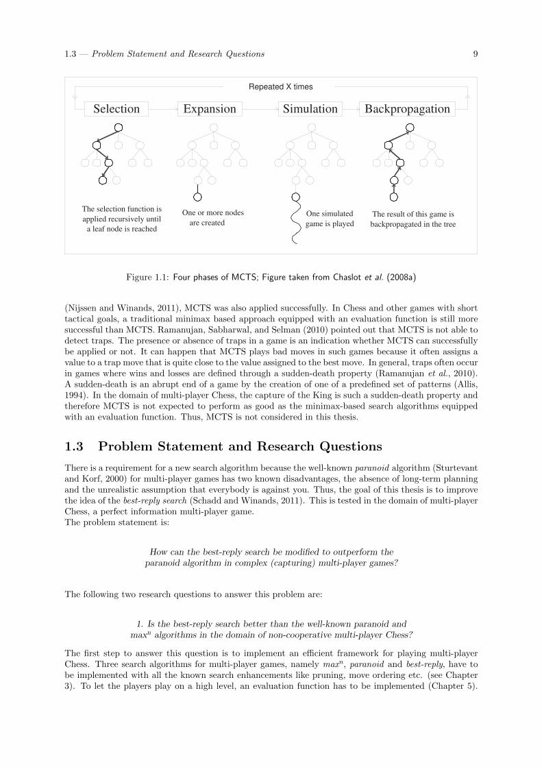
Monte-Carlo Tree Search (MCTS) (Coulom, 2007; Kocsis and Szepesvari, 2006) does not build a gametree of a fixed depth and does not use an evaluation function to assign values to the leaf nodes as theprevious search algorithms. Instead, it is a best-first algorithm based on randomized explorations of thesearch space (Chaslot et al., 2008a). “Using the results of previous explorations, the algorithm graduallygrows a game tree in memory, and successively becomes better at accurately estimating the values of themost promising moves” (Chaslot, Winands, and Van den Herik, 2008b). Figure 1.1 illustrates the fourphases of MCTS.
1. SelectionIn this phase, the tree is traversed from the root node until it selects a node not added to the treeso far.
2. ExpansionIn this phase, the node selected in the previous phase is added to the tree.
3. SimulationIn this phase, moves are played until the end of the game is reached. The result of this search canbe a win, a draw or a loss for the root player.
4. BackpropagationIn this phase, the result of the simulation is propagated through the tree.
MCTS has become popular in the area of games (Browne et al., 2012). Examples for two-player gameswhere it has successfully been applied are Go (Chaslot et al., 2008a; Coulom, 2007), Amazons (Lorentz,2008), Lines of Action (Winands and Bjornsson, 2010) and Hex (Cazenave and Saffidine, 2009). In themulti-player games Chinese Checkers (Sturtevant, 2008), multi-player Go (Cazenave, 2008) and Focus
1.3 — Problem Statement and Research Questions 9
Selection Expension Simulation Backpropagation
The selection function is applied
recursively until a leaf node is
reached
One or more nodes
are created The result of this game is
backpropagated in the tree
One simulated
game is played
Selection Expansion Simulation Backpropagation
The selection function is
applied recursively until
a leaf node is reached
One or more nodes
are created The result of this game is
backpropagated in the tree
One simulated
game is played
Repeated X times
Figure 1.1: Four phases of MCTS; Figure taken from Chaslot et al. (2008a)
(Nijssen and Winands, 2011), MCTS was also applied successfully. In Chess and other games with shorttactical goals, a traditional minimax based approach equipped with an evaluation function is still moresuccessful than MCTS. Ramanujan, Sabharwal, and Selman (2010) pointed out that MCTS is not able todetect traps. The presence or absence of traps in a game is an indication whether MCTS can successfullybe applied or not. It can happen that MCTS plays bad moves in such games because it often assigns avalue to a trap move that is quite close to the value assigned to the best move. In general, traps often occurin games where wins and losses are defined through a sudden-death property (Ramanujan et al., 2010).A sudden-death is an abrupt end of a game by the creation of one of a predefined set of patterns (Allis,1994). In the domain of multi-player Chess, the capture of the King is such a sudden-death property andtherefore MCTS is not expected to perform as good as the minimax-based search algorithms equippedwith an evaluation function. Thus, MCTS is not considered in this thesis.
1.3 Problem Statement and Research Questions
There is a requirement for a new search algorithm because the well-known paranoid algorithm (Sturtevantand Korf, 2000) for multi-player games has two known disadvantages, the absence of long-term planningand the unrealistic assumption that everybody is against you. Thus, the goal of this thesis is to improvethe idea of the best-reply search (Schadd and Winands, 2011). This is tested in the domain of multi-playerChess, a perfect information multi-player game.The problem statement is:
How can the best-reply search be modified to outperform theparanoid algorithm in complex (capturing) multi-player games?
The following two research questions to answer this problem are:
1. Is the best-reply search better than the well-known paranoid andmaxn algorithms in the domain of non-cooperative multi-player Chess?
The first step to answer this question is to implement an efficient framework for playing multi-playerChess. Three search algorithms for multi-player games, namely maxn, paranoid and best-reply, have tobe implemented with all the known search enhancements like pruning, move ordering etc. (see Chapter3). To let the players play on a high level, an evaluation function has to be implemented (Chapter 5).
10 Introduction
Finally, the developed framework can be used to check the performance of the best-reply search againstthe two other algorithms.
2. Can we find variants of the best-reply search that are even better?
To answer this question first the weaknesses of the best-reply search has to be discussed. Ideas to over-come these weaknesses are proposed (see Chapter 4) and implemented. The main idea proposed in thisthesis is to let the passing opponents play the best move from the static move ordering. Further, thenumber of searching players can be varied. Finally, experiments have to be executed to find out whichvariant of the best-reply search is the strongest one and how does it perform against the paranoid andmaxn algorithms in the domain of multi-player Chess.
1.4 Outline of the Thesis
Here a brief outline of the thesis is given.
• Chapter 1 gives an introduction to artificial intelligence in multi-player games. Further, the problemstatement and research questions are stated.
• Chapter 2 describes the game of multi-player Chess.
• Chapter 3 explains the search techniques used in the program.
• Chapter 4 describes the proposed best-reply search variants.
• Chapter 5 discusses the evaluation function required to assign values to the leaf nodes of the gametree.
• Chapter 6 explains the performed experiments and presents the corresponding results.
• Chapter 7 presents the conclusion of this thesis and the future research.
Chapter 2
Multi-Player Chess
This chapter describes the game of multi-player Chess which is used as test domain in this thesis. Section2.1 gives an introduction to regular Chess. Section 2.2 explains multi-player Chess itself. In Section 2.3,the complexity of multi-player Chess is computed.
2.1 Two-Player Chess
An insight into the history of Chess is given in Subsection 2.1.1. The rules of regular Chess are explainedfrom Subsection 2.1.2 through to 2.1.5
2.1.1 History
The earliest predecessors of Chess originated before the 6th century in India. From India, the gamespread to Persia where they started calling “Shah!” (Persian for “King!”) when threaten the opponent’sKing, and “Shah Mat” (Persian for “the King is helpless”) when the King can not escape from attack.These exclamations persisted in Chess, e.g., nowadays in Germany the exclamations are still “Schach!”and “Schach Matt!”. When the Arabs conquered Persia, Chess was taken up by the Muslim world andsubsequently spread to Europe and Russia at the end of the first millennium. In the 15th century, theBishop’s and Queen’s moves were changed and Chess became close to its current form. Also the firstwritings about the theory of playing Chess appeared in that century. In the 19th century many Chessclubs, Chess books and Chess journals appeared and the first modern Chess tournament play began. Thefirst World Chess Championship was held in 1886. Position analysis became also popular during thistime.
2.1.2 Board and Initial Position
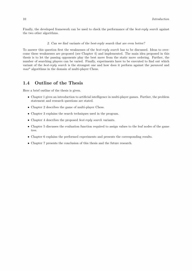
Figure 2.1: Initial Position in Chess
Chess is played on an 8 × 8 board. The players are calledWhite and Black. Both players start with 16 pieces as shownin Figure 2.1. Each player has eight Pawns , two Rooks ,two Knights , two Bishops , one Queen and one King
.
2.1.3 Movement
The players move alternately, starting with White. Movingmeans that the player moves one of his pieces to an emptysquare or a square with an opponent piece on it. If the squarehas an opponent’s piece on it, this piece gets removed from theboard. In general it is not allowed to jump over other pieces.Only the Knight is allowed to do this. Each kind of piece has itsown rules how it is allowed to move. These individual movingrules are as follows.
12 Multi-Player Chess
(a) Movement of allwhite Pawns
(b) Rook’s movement (c) Knight’s movement
(d) Bishop’s movement (e) Queen’s movement (f) King’s movement
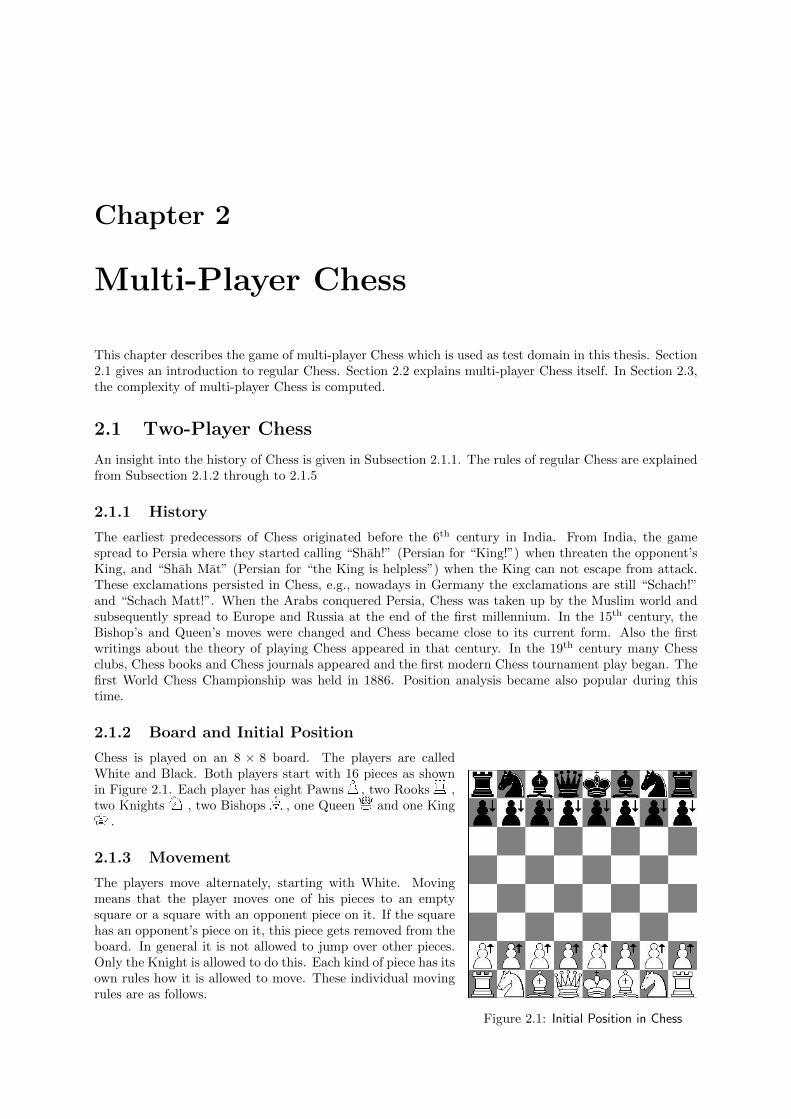
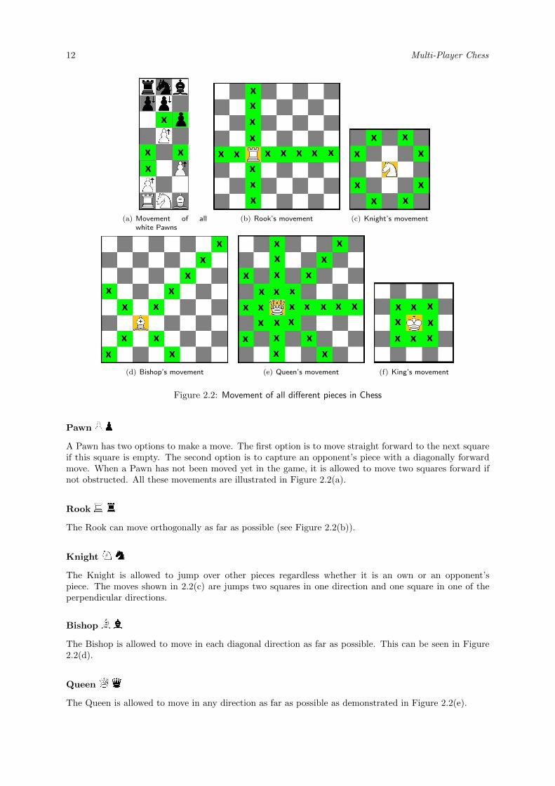
Figure 2.2: Movement of all different pieces in Chess
Pawn
A Pawn has two options to make a move. The first option is to move straight forward to the next squareif this square is empty. The second option is to capture an opponent’s piece with a diagonally forwardmove. When a Pawn has not been moved yet in the game, it is allowed to move two squares forward ifnot obstructed. All these movements are illustrated in Figure 2.2(a).
Rook
The Rook can move orthogonally as far as possible (see Figure 2.2(b)).
Knight
The Knight is allowed to jump over other pieces regardless whether it is an own or an opponent’spiece. The moves shown in 2.2(c) are jumps two squares in one direction and one square in one of theperpendicular directions.
Bishop
The Bishop is allowed to move in each diagonal direction as far as possible. This can be seen in Figure2.2(d).
Queen
The Queen is allowed to move in any direction as far as possible as demonstrated in Figure 2.2(e).
2.1 — Two-Player Chess 13
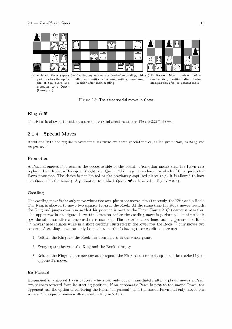
(a) A black Pawn (upperpart) reaches the oppo-site of the board andpromotes to a Queen(lower part)
(b) Castling, upper row: position before castling, mid-dle row: position after long castling, lower row:position after short castling
(c) En Passant Move; position beforedouble step, position after doublestep,position after en-passant move
Figure 2.3: The three special moves in Chess
King
The King is allowed to make a move to every adjacent square as Figure 2.2(f) shows.
2.1.4 Special Moves
Additionally to the regular movement rules there are three special moves, called promotion, castling anden-passant.
Promotion
A Pawn promotes if it reaches the opposite side of the board. Promotion means that the Pawn getsreplaced by a Rook, a Bishop, a Knight or a Queen. The player can choose to which of these pieces thePawn promotes. The choice is not limited to the previously captured pieces (e.g., it is allowed to have
two Queens on the board). A promotion to a black Queen is depicted in Figure 2.3(a).
Castling
The castling move is the only move where two own pieces are moved simultaneously, the King and a Rook.The King is allowed to move two squares towards the Rook. At the same time the Rook moves towardsthe King and jumps over him so that his position is next to the King. Figure 2.3(b) demonstrates this.The upper row in the figure shows the situation before the castling move is performed. In the middlerow the situation after a long castling is mapped. This move is called long castling because the Rook
moves three squares while in a short castling illustrated in the lower row the Rook only moves twosquares. A castling move can only be made when the following three conditions are met:
1. Neither the King nor the Rook has been moved in the whole game.
2. Every square between the King and the Rook is empty.
3. Neither the Kings square nor any other square the King passes or ends up in can be reached by anopponent’s move.
En-Passant
En-passant is a special Pawn capture which can only occur immediately after a player moves a Pawntwo squares forward from its starting position. If an opponent’s Pawn is next to the moved Pawn, theopponent has the option of capturing the Pawn “en passant” as if the moved Pawn had only moved onesquare. This special move is illustrated in Figure 2.3(c).
14 Multi-Player Chess
2.1.5 End of the Game
The sole objective of the game is to capture the opponent’s King. A move that threatens to capture theKing is called a check move. The opponent has to react to this move. If the opponent cannot play amove to prevent his King from being captured, he is checkmate and loses the game. The game can alsoend in a draw when one of the following three conditions are met:
1. No progression, which means that no piece has been captured and no Pawn has been moved in thelast 50 moves.
2. An identical position, including the player on turn, occurs for the third time.
3. The player on turn has no legal move and is not in check. This situation is called Stalemate.
2.2 Multi-Player Chess
In this section the history of multi-player Chess is outlined in Subsection 2.2.1. The supplemental rulesare revealed from Subsection 2.2.2 through to 2.2.7. The multi-player Chess rules used in this thesis aretaken over from Tscheuschner (2005).
2.2.1 History
Chess variants for more than two players have been invented for more than two hundred years. The boardsize was increased, depending on the variant by adding two to four rows to each side. The pieces usedfor each player are in nearly all variants the same as for regular Chess. But there are many different rulevariations of multi-player Chess. The most common form of play is cooperative (two vs. two) in whichallied pieces cannot eliminate each other. The game is over when both opposing Kings are checkmated.Playing non-cooperative is generally regarded more difficult than team play. Each player can attack anyof the other three players and vice versa. Once a player is checkmated, depending on the variant eitherthe pieces of the checkmated player gets removed from the board, or the player that checkmated can usethe remaining pieces during his turn. For more information about multi-player Chess variants and Chessvariants in general see Pritchard (2001). Non-cooperative play with removing the pieces of the defeatedopponent is used in this thesis.
2.2.2 Board and Initial Position
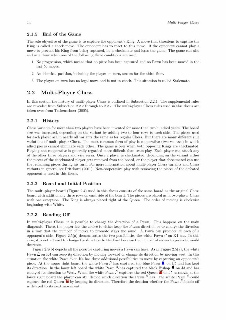
The multi-player board (Figure 2.4) used in this thesis consists of the same board as the original Chessboard with additionally three rows on each side of the board. The pieces are placed as in two-player Chesswith one exception. The King is always placed right of the Queen. The order of moving is clockwisebeginning with White.
2.2.3 Bending Off
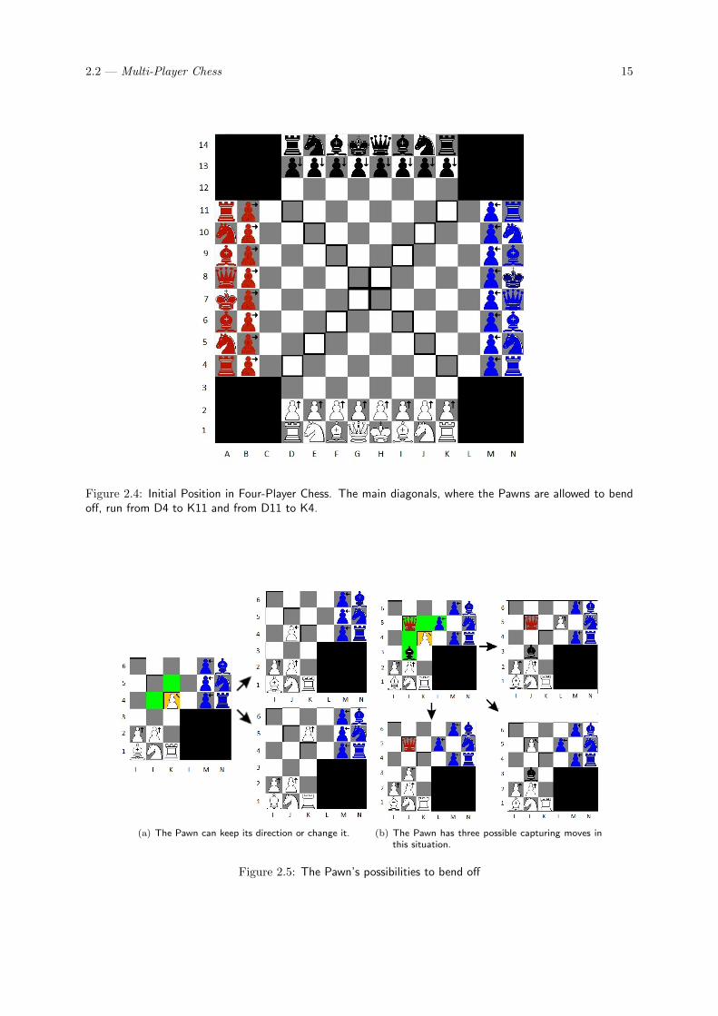
In multi-player Chess, it is possible to change the direction of a Pawn. This happens on the maindiagonals. There, the player has the choice to either keep the Pawns direction or to change the directionin a way that the number of moves to promote stays the same. A Pawn can promote at each of aopponent’s side. Figure 2.5(a) demonstrates the two possibilities the white Pawn on K4 has. In thiscase, it is not allowed to change the direction to the East because the number of moves to promote woulddecrease.
Figure 2.5(b) depicts all the possible capturing moves a Pawn can have. As in Figure 2.5(a), the white
Pawn on K4 can keep its direction by moving forward or change its direction by moving west. In thissituation the white Pawn on K4 has three additional possibilities to move by capturing an opponent’spiece. At the upper right board the white Pawn has captured the blue Pawn on L5 and has keptits direction. In the lower left board the white Pawn has captured the black Bishop on J3 and haschanged its direction to West. When the white Pawn captures the red Queen on J5 as shown at thelower right board the player can still decide which direction the Pawn has. The white Pawn couldcapture the red Queen by keeping its direction. Therefore the decision whether the Pawn bends offis delayed to its next movement.
2.2 — Multi-Player Chess 15
Figure 2.4: Initial Position in Four-Player Chess. The main diagonals, where the Pawns are allowed to bendoff, run from D4 to K11 and from D11 to K4.
(a) The Pawn can keep its direction or change it. (b) The Pawn has three possible capturing moves inthis situation.
Figure 2.5: The Pawn’s possibilities to bend off
16 Multi-Player Chess
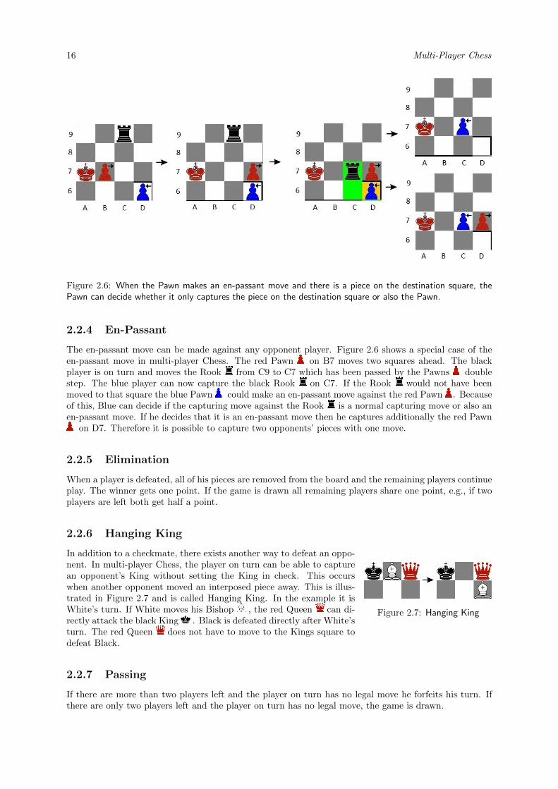
Figure 2.6: When the Pawn makes an en-passant move and there is a piece on the destination square, thePawn can decide whether it only captures the piece on the destination square or also the Pawn.
2.2.4 En-Passant
The en-passant move can be made against any opponent player. Figure 2.6 shows a special case of theen-passant move in multi-player Chess. The red Pawn on B7 moves two squares ahead. The blackplayer is on turn and moves the Rook from C9 to C7 which has been passed by the Pawns doublestep. The blue player can now capture the black Rook on C7. If the Rook would not have beenmoved to that square the blue Pawn could make an en-passant move against the red Pawn . Becauseof this, Blue can decide if the capturing move against the Rook is a normal capturing move or also anen-passant move. If he decides that it is an en-passant move then he captures additionally the red Pawn
on D7. Therefore it is possible to capture two opponents’ pieces with one move.
2.2.5 Elimination
When a player is defeated, all of his pieces are removed from the board and the remaining players continueplay. The winner gets one point. If the game is drawn all remaining players share one point, e.g., if twoplayers are left both get half a point.
2.2.6 Hanging King
Figure 2.7: Hanging King
In addition to a checkmate, there exists another way to defeat an oppo-nent. In multi-player Chess, the player on turn can be able to capturean opponent’s King without setting the King in check. This occurswhen another opponent moved an interposed piece away. This is illus-trated in Figure 2.7 and is called Hanging King. In the example it isWhite’s turn. If White moves his Bishop , the red Queen can di-rectly attack the black King . Black is defeated directly after White’sturn. The red Queen does not have to move to the Kings square todefeat Black.
2.2.7 Passing
If there are more than two players left and the player on turn has no legal move he forfeits his turn. Ifthere are only two players left and the player on turn has no legal move, the game is drawn.
2.3 — Complexity 17
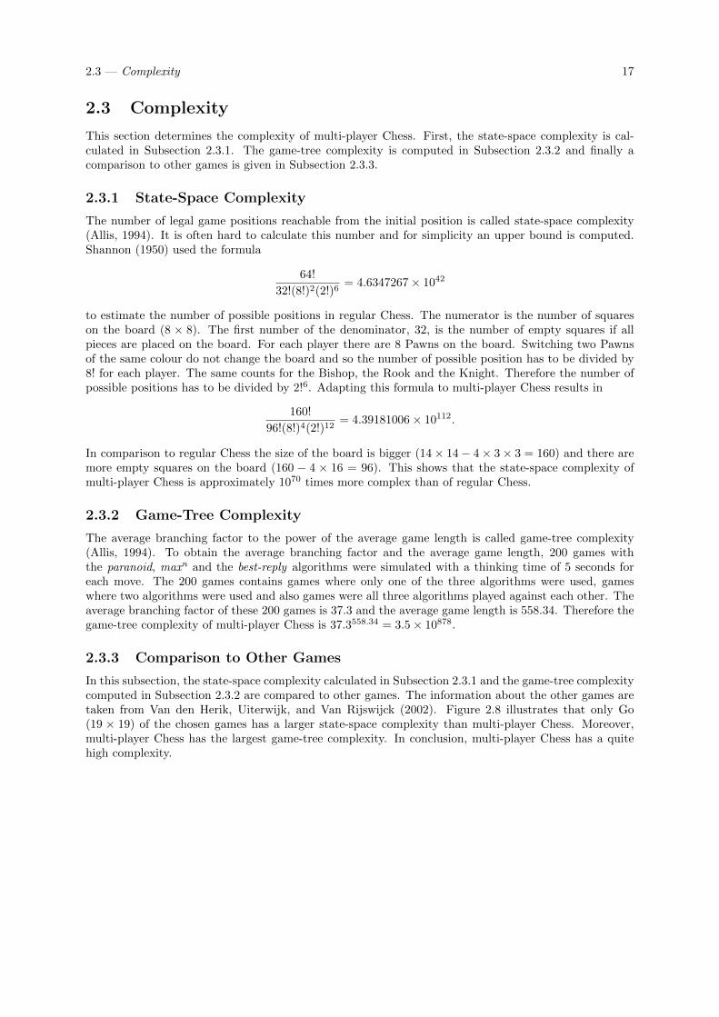
2.3 Complexity
This section determines the complexity of multi-player Chess. First, the state-space complexity is cal-culated in Subsection 2.3.1. The game-tree complexity is computed in Subsection 2.3.2 and finally acomparison to other games is given in Subsection 2.3.3.
2.3.1 State-Space Complexity
The number of legal game positions reachable from the initial position is called state-space complexity(Allis, 1994). It is often hard to calculate this number and for simplicity an upper bound is computed.Shannon (1950) used the formula
64!
32!(8!)2(2!)6= 4.6347267× 1042
to estimate the number of possible positions in regular Chess. The numerator is the number of squareson the board (8 × 8). The first number of the denominator, 32, is the number of empty squares if allpieces are placed on the board. For each player there are 8 Pawns on the board. Switching two Pawnsof the same colour do not change the board and so the number of possible position has to be divided by8! for each player. The same counts for the Bishop, the Rook and the Knight. Therefore the number ofpossible positions has to be divided by 2!6. Adapting this formula to multi-player Chess results in
160!
96!(8!)4(2!)12= 4.39181006× 10112.
In comparison to regular Chess the size of the board is bigger (14× 14− 4× 3× 3 = 160) and there aremore empty squares on the board (160 − 4 × 16 = 96). This shows that the state-space complexity ofmulti-player Chess is approximately 1070 times more complex than of regular Chess.
2.3.2 Game-Tree Complexity
The average branching factor to the power of the average game length is called game-tree complexity(Allis, 1994). To obtain the average branching factor and the average game length, 200 games withthe paranoid, maxn and the best-reply algorithms were simulated with a thinking time of 5 seconds foreach move. The 200 games contains games where only one of the three algorithms were used, gameswhere two algorithms were used and also games were all three algorithms played against each other. Theaverage branching factor of these 200 games is 37.3 and the average game length is 558.34. Therefore thegame-tree complexity of multi-player Chess is 37.3558.34 = 3.5× 10878.
2.3.3 Comparison to Other Games
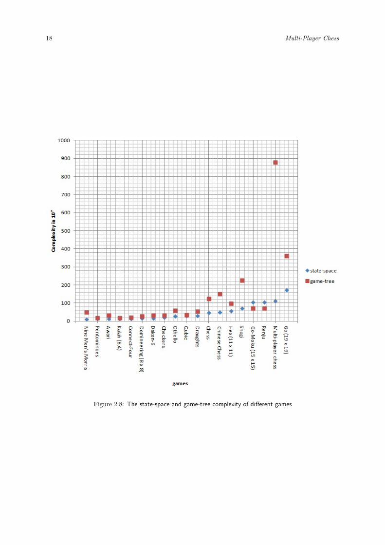
In this subsection, the state-space complexity calculated in Subsection 2.3.1 and the game-tree complexitycomputed in Subsection 2.3.2 are compared to other games. The information about the other games aretaken from Van den Herik, Uiterwijk, and Van Rijswijck (2002). Figure 2.8 illustrates that only Go(19 × 19) of the chosen games has a larger state-space complexity than multi-player Chess. Moreover,multi-player Chess has the largest game-tree complexity. In conclusion, multi-player Chess has a quitehigh complexity.
18 Multi-Player Chess
Figure 2.8: The state-space and game-tree complexity of different games
Chapter 3
Search Techniques
As explained in Subsection 2.3.1, multi-player Chess is quite complex and therefore it is not possibleto assign a decision to each possible board position. An evaluation function (described in Chapter 5) isregarded to assign a value to each leaf node in the game tree (see Section 1.2). Moreover, a decision rule isrequired which defines how the values of the leaf nodes are propagated up the game tree. The evaluationfunction and the decision rule dictate the strategy of a player (Sturtevant, 2003a). Evaluation functionsare domain dependent which means that an evaluation function for e.g., Chess cannot be reused for othergames. But the generic decision rules can be used for many games. First in this chapter, a decision rulecalled minimax for two-player games is explained in Section 3.1. Enhancements of this decision rule areexplained in Section 3.2. Decision rules for multi-player games are explained in Section 3.3 and quiescencesearch is described in Section 3.4.
3.1 Two-Player Search Algorithms
In the following, the most popular algorithm for two-player games, called minimax, is described. Further,αβ-pruning is explained.
3.1.1 Minimax
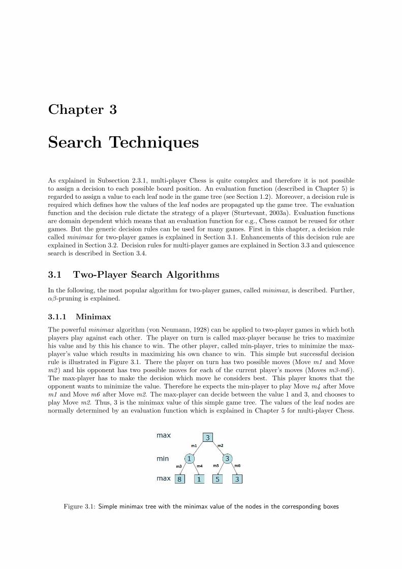
The powerful minimax algorithm (von Neumann, 1928) can be applied to two-player games in which bothplayers play against each other. The player on turn is called max-player because he tries to maximizehis value and by this his chance to win. The other player, called min-player, tries to minimize the max-player’s value which results in maximizing his own chance to win. This simple but successful decisionrule is illustrated in Figure 3.1. There the player on turn has two possible moves (Move m1 and Movem2 ) and his opponent has two possible moves for each of the current player’s moves (Moves m3-m6 ).The max-player has to make the decision which move he considers best. This player knows that theopponent wants to minimize the value. Therefore he expects the min-player to play Move m4 after Movem1 and Move m6 after Move m2. The max-player can decide between the value 1 and 3, and chooses toplay Move m2. Thus, 3 is the minimax value of this simple game tree. The values of the leaf nodes arenormally determined by an evaluation function which is explained in Chapter 5 for multi-player Chess.
Figure 3.1: Simple minimax tree with the minimax value of the nodes in the corresponding boxes
20 Search Techniques
The values of the other nodes are propagated up the tree as explained above. The pseudo-code for thisalgorithm can be seen in Algorithm 3.1.1. Usually, it is not possible to search the complete game treeand therefore a parameter defines the search depth of the algorithm.
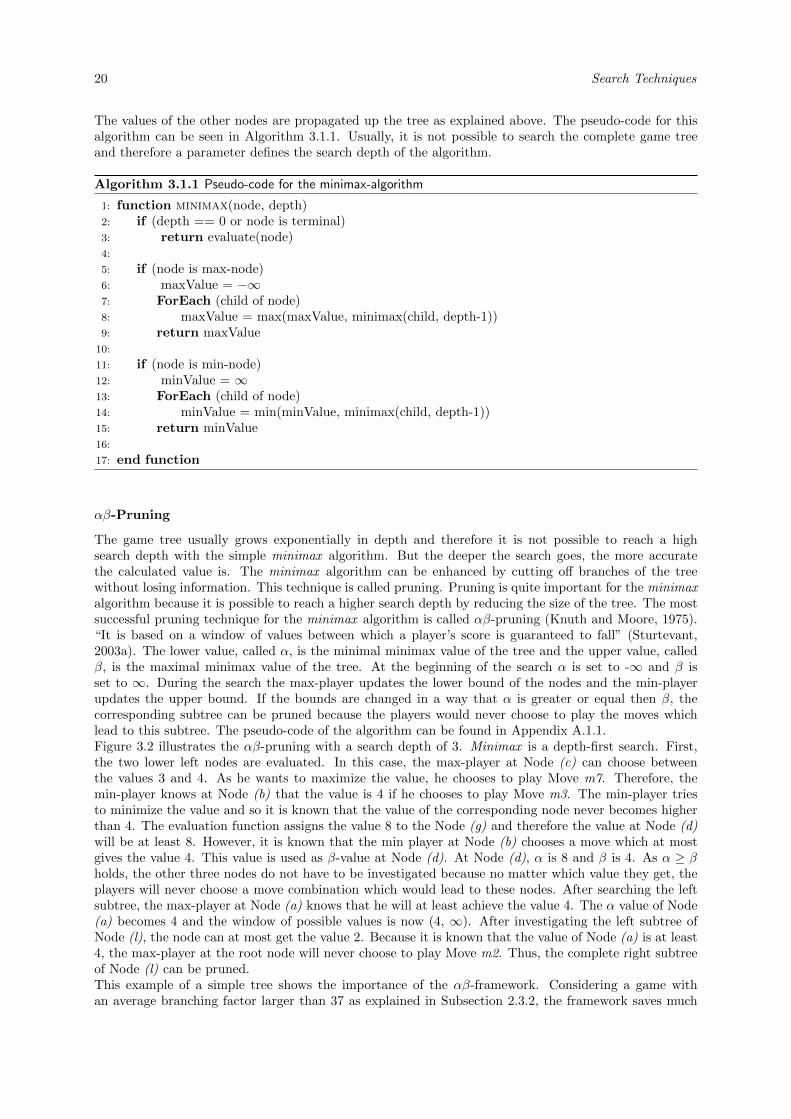
Algorithm 3.1.1 Pseudo-code for the minimax-algorithm
1: function minimax(node, depth)2: if (depth == 0 or node is terminal)3: return evaluate(node)4:
5: if (node is max-node)6: maxValue = −∞7: ForEach (child of node)8: maxValue = max(maxValue, minimax(child, depth-1))9: return maxValue
10:
11: if (node is min-node)12: minValue = ∞13: ForEach (child of node)14: minValue = min(minValue, minimax(child, depth-1))15: return minValue16:
17: end function
αβ-Pruning
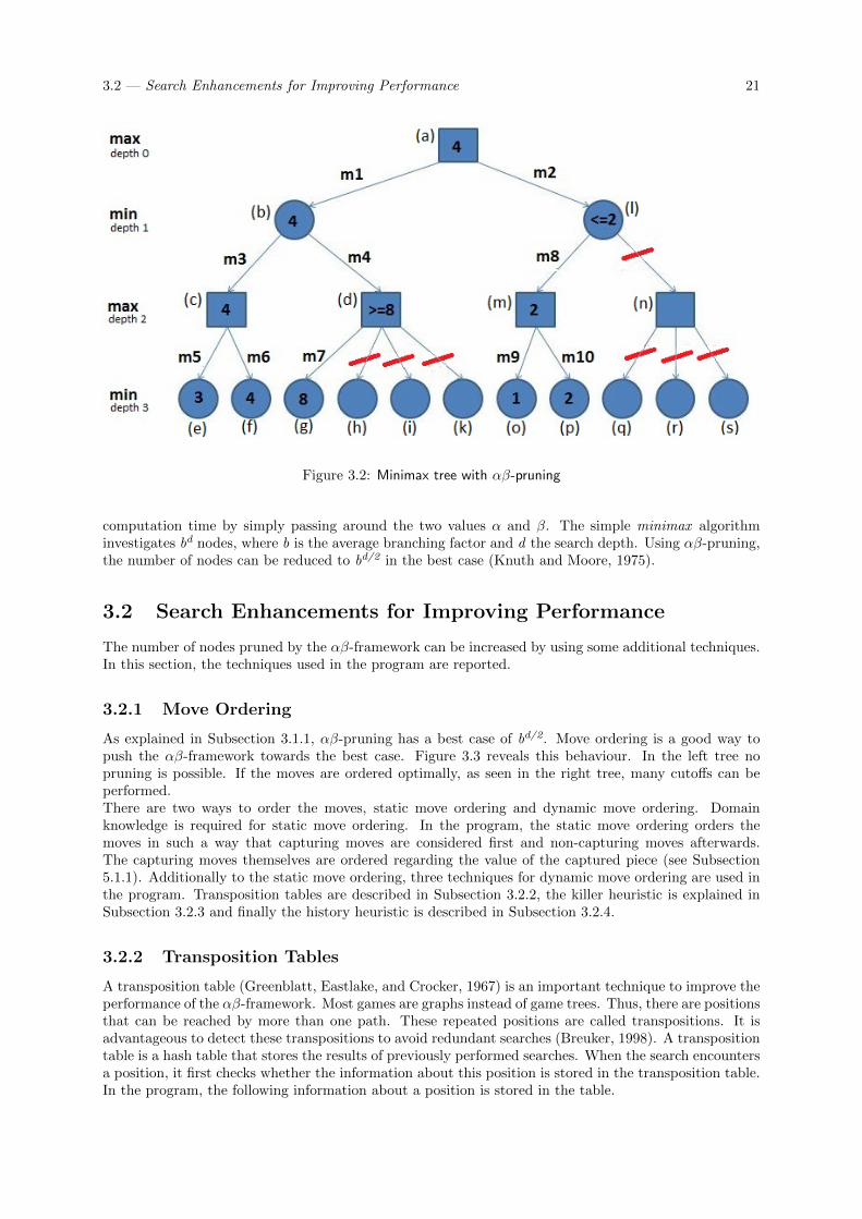
The game tree usually grows exponentially in depth and therefore it is not possible to reach a highsearch depth with the simple minimax algorithm. But the deeper the search goes, the more accuratethe calculated value is. The minimax algorithm can be enhanced by cutting off branches of the treewithout losing information. This technique is called pruning. Pruning is quite important for the minimaxalgorithm because it is possible to reach a higher search depth by reducing the size of the tree. The mostsuccessful pruning technique for the minimax algorithm is called αβ-pruning (Knuth and Moore, 1975).“It is based on a window of values between which a player’s score is guaranteed to fall” (Sturtevant,2003a). The lower value, called α, is the minimal minimax value of the tree and the upper value, calledβ, is the maximal minimax value of the tree. At the beginning of the search α is set to -∞ and β isset to ∞. During the search the max-player updates the lower bound of the nodes and the min-playerupdates the upper bound. If the bounds are changed in a way that α is greater or equal then β, thecorresponding subtree can be pruned because the players would never choose to play the moves whichlead to this subtree. The pseudo-code of the algorithm can be found in Appendix A.1.1.Figure 3.2 illustrates the αβ-pruning with a search depth of 3. Minimax is a depth-first search. First,the two lower left nodes are evaluated. In this case, the max-player at Node (c) can choose betweenthe values 3 and 4. As he wants to maximize the value, he chooses to play Move m7. Therefore, themin-player knows at Node (b) that the value is 4 if he chooses to play Move m3. The min-player triesto minimize the value and so it is known that the value of the corresponding node never becomes higherthan 4. The evaluation function assigns the value 8 to the Node (g) and therefore the value at Node (d)will be at least 8. However, it is known that the min player at Node (b) chooses a move which at mostgives the value 4. This value is used as β-value at Node (d). At Node (d), α is 8 and β is 4. As α ≥ βholds, the other three nodes do not have to be investigated because no matter which value they get, theplayers will never choose a move combination which would lead to these nodes. After searching the leftsubtree, the max-player at Node (a) knows that he will at least achieve the value 4. The α value of Node(a) becomes 4 and the window of possible values is now (4, ∞). After investigating the left subtree ofNode (l), the node can at most get the value 2. Because it is known that the value of Node (a) is at least4, the max-player at the root node will never choose to play Move m2. Thus, the complete right subtreeof Node (l) can be pruned.This example of a simple tree shows the importance of the αβ-framework. Considering a game withan average branching factor larger than 37 as explained in Subsection 2.3.2, the framework saves much
3.2 — Search Enhancements for Improving Performance 21
Figure 3.2: Minimax tree with αβ-pruning
computation time by simply passing around the two values α and β. The simple minimax algorithminvestigates bd nodes, where b is the average branching factor and d the search depth. Using αβ-pruning,the number of nodes can be reduced to bd/2 in the best case (Knuth and Moore, 1975).
3.2 Search Enhancements for Improving Performance
The number of nodes pruned by the αβ-framework can be increased by using some additional techniques.In this section, the techniques used in the program are reported.
3.2.1 Move Ordering
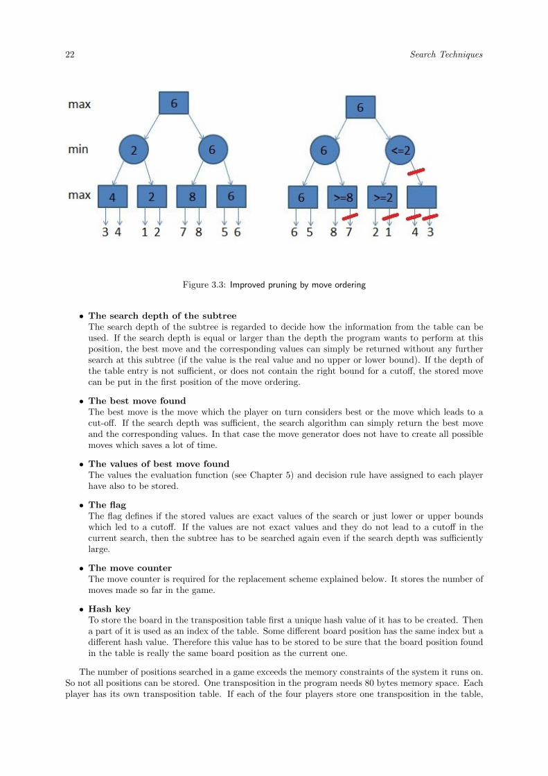
As explained in Subsection 3.1.1, αβ-pruning has a best case of bd/2. Move ordering is a good way topush the αβ-framework towards the best case. Figure 3.3 reveals this behaviour. In the left tree nopruning is possible. If the moves are ordered optimally, as seen in the right tree, many cutoffs can beperformed.There are two ways to order the moves, static move ordering and dynamic move ordering. Domainknowledge is required for static move ordering. In the program, the static move ordering orders themoves in such a way that capturing moves are considered first and non-capturing moves afterwards.The capturing moves themselves are ordered regarding the value of the captured piece (see Subsection5.1.1). Additionally to the static move ordering, three techniques for dynamic move ordering are used inthe program. Transposition tables are described in Subsection 3.2.2, the killer heuristic is explained inSubsection 3.2.3 and finally the history heuristic is described in Subsection 3.2.4.
3.2.2 Transposition Tables
A transposition table (Greenblatt, Eastlake, and Crocker, 1967) is an important technique to improve theperformance of the αβ-framework. Most games are graphs instead of game trees. Thus, there are positionsthat can be reached by more than one path. These repeated positions are called transpositions. It isadvantageous to detect these transpositions to avoid redundant searches (Breuker, 1998). A transpositiontable is a hash table that stores the results of previously performed searches. When the search encountersa position, it first checks whether the information about this position is stored in the transposition table.In the program, the following information about a position is stored in the table.
22 Search Techniques
Figure 3.3: Improved pruning by move ordering
• The search depth of the subtreeThe search depth of the subtree is regarded to decide how the information from the table can beused. If the search depth is equal or larger than the depth the program wants to perform at thisposition, the best move and the corresponding values can simply be returned without any furthersearch at this subtree (if the value is the real value and no upper or lower bound). If the depth ofthe table entry is not sufficient, or does not contain the right bound for a cutoff, the stored movecan be put in the first position of the move ordering.
• The best move foundThe best move is the move which the player on turn considers best or the move which leads to acut-off. If the search depth was sufficient, the search algorithm can simply return the best moveand the corresponding values. In that case the move generator does not have to create all possiblemoves which saves a lot of time.
• The values of best move foundThe values the evaluation function (see Chapter 5) and decision rule have assigned to each playerhave also to be stored.
• The flagThe flag defines if the stored values are exact values of the search or just lower or upper boundswhich led to a cutoff. If the values are not exact values and they do not lead to a cutoff in thecurrent search, then the subtree has to be searched again even if the search depth was sufficientlylarge.
• The move counterThe move counter is required for the replacement scheme explained below. It stores the number ofmoves made so far in the game.
• Hash keyTo store the board in the transposition table first a unique hash value of it has to be created. Thena part of it is used as an index of the table. Some different board position has the same index but adifferent hash value. Therefore this value has to be stored to be sure that the board position foundin the table is really the same board position as the current one.
The number of positions searched in a game exceeds the memory constraints of the system it runs on.So not all positions can be stored. One transposition in the program needs 80 bytes memory space. Eachplayer has its own transposition table. If each of the four players store one transposition in the table,
3.2 — Search Enhancements for Improving Performance 23
320 Bytes memory is required. In the program each player is allowed to store 219 = 524288 entries in histable. Therefore, the maximum space for the transposition tables is roughly 170 MB. To store the values,the board position has to be transformed into a hash value, in the program a value of 64 bits. The last19 bits are used as the index of the hash table. Zobrist hashing (Zobrist, 1970) is used to calculate thisvalue. With Zobrist hashing it is possible to update the hash value incrementally which makes it fast.If a new position is reached in the game and the last 19 bits of the hash value of this board is alreadyused as index in the transposition table, then a replacement strategy is needed to decide which of theboard position should be stored in the table. Therefore the move counter is stored in the transpositiontable. Even if the board stored in the transposition table has a larger search depth than the currentboard position, the current board position can replace the old one when the old position occurred in aprevious search. In this thesis, the new value is stored if the length of the path leading to the positionplus the depth of the subtree is bigger or equal than the corresponding value of the stored position.There exists one problem in the application of transposition tables for some games - also regular Chessand multi-player Chess - called Graph-History-Interaction Problem (Campbell, 1985) which was solvedby Kishimoto and Muller (2004). This problem occurs when the position is evaluated differently whenreached via different paths. In multi-player Chess, there is a problem regarding the rule explained inSubsection 2.1.5 that the game is over if a board has repeated for the third time. The transpositiontable is in general not able to detect how often a position occurred and so a player in a winning positioncould play the best move stored in the transposition table even if this move would lead to a draw. In theprogram the problem is tackled by also using the number of same board positions so far to calculate thehash key of the position.
3.2.3 Killer Heuristic
The killer heuristic (Akl and Newborn, 1977) is a dynamic move ordering technique that improves theefficiency of αβ-pruning. Killer moves rely on the assumption that most moves do not change the boardposition too much. The killer heuristic tries to produce an early cutoff by first considering a legal movethat led to a cutoff in another branch of the tree at the same depth. In the program, three moves perply are stored as killer moves. If a non-killer move leads to a cutoff, it replaces the oldest killer move ofthat ply and becomes the killer move considered first at the next search of that ply. It is good to havemore than one killer move per ply because it prevents from forgetting a good killer move to early.
3.2.4 History Heuristic
The dynamic move ordering technique called history heuristic was invented by Schaeffer (1983). At thebeginning of a game, a table of all possible moves in the game has to be created. In multi-player Chess,there are 160 squares on the board and therefore a table of size 160× 160 is required to store one valuefor each possible move. The piece type making the move is not considered. All values of the table areset to 0 at the beginning. At every internal node, the table entry for the best move found at that nodegets incremented by a value. The added value can freely be chosen but typically it depends on the depthof the subtree because the deeper the search depth is, the more accurate the best move is. Two popularapproaches are to use 2depth or depth2. In the program the last version is used and the values from thetable are used to order the non-capturing moves. The values in the table can be maintained over thewhole game. Each time a player has to make a new move the scores in the table are decremented bya factor. In the program the values are divided by 10. The history heuristic has some disadvantages.One of them is that the history heuristic is biased towards moves that occur more often in a game thanothers (Hartmann, 1988). To overcome this disadvantage, a relative history heuristic can be applied(Winands et al., 2006).
3.2.5 Iterative Deepening
Iterative deepening (De Groot, 1965) breaks the search process into multiple iterations. Each iterationsearches to a greater depth than the previous iteration (Russell and Norvig, 2010). Iterative deepening isused as a time management strategy. Each player in the game gets an amount of time for finding a moveinstead of a searching to a fixed depth. This is quite important for comparing the strength of differentdecision rules like maxn (see Subsection 3.3.1) and paranoid (Subsection 3.3.2). It was shown that this
24 Search Techniques
technique is also beneficial in the αβ-framework because the result of the last iteration can be used forthe dynamic move ordering in the new iteration which often leads to an early cutoff. When the time forsearching is over, the algorithm stops the search at the current depth. In this thesis, the best move fromthe previous search depth is played. In general, it is also possible to use the information gained from thepartial search at the current depth. The best move from the previous depth is searched first and thus,the value of this move is known first. When another move results in a higher value, it can replace thebest move and be played when the time for searching is over.
3.3 Multi-Player Search Algorithms
In this section the decision rules for deterministic multi-player games with perfect information are de-scribed. First maxn is described in Subsection 3.3.1, then paranoid is described in Subsection 3.3.2 andfinally best-reply search is explained in Subsection 3.3.3.
3.3.1 Maxn
Maxn (Luckhart and Irani, 1986) is the generalization of the minimax algorithm for multi-player gameswith n players (Sturtevant, 2003a). The root player assumes that each player tries to maximize his ownscore. The leaf nodes of the tree have n instead of just one value, where the ith value represents the scoreof the ith player. The pseudo-code can be seen in Algorithm 3.3.1.
Algorithm 3.3.1 Pseudo-code for the maxn-algorithm
1: function maxN(node, depth)2: if (depth == 0 or node is terminal)3: return evaluate(node)4: maxValues = maxN(firstChild, depth-1)5: ForEach (child of node)6: values = maxN(child, depth-1)7: if (values[playerOnTurn] > maxValues[playerOnTurn])8: maxValues = values9:
10: return maxValues11: end function
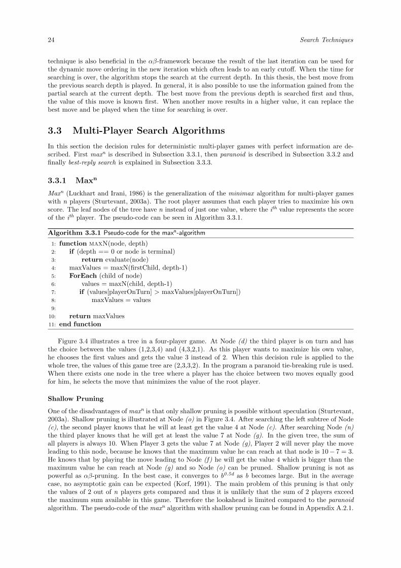
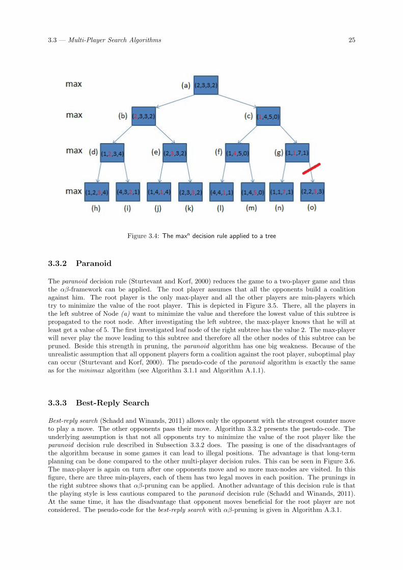
Figure 3.4 illustrates a tree in a four-player game. At Node (d) the third player is on turn and hasthe choice between the values (1,2,3,4) and (4,3,2,1). As this player wants to maximize his own value,he chooses the first values and gets the value 3 instead of 2. When this decision rule is applied to thewhole tree, the values of this game tree are (2,3,3,2). In the program a paranoid tie-breaking rule is used.When there exists one node in the tree where a player has the choice between two moves equally goodfor him, he selects the move that minimizes the value of the root player.
Shallow Pruning
One of the disadvantages of maxn is that only shallow pruning is possible without speculation (Sturtevant,2003a). Shallow pruning is illustrated at Node (o) in Figure 3.4. After searching the left subtree of Node(c), the second player knows that he will at least get the value 4 at Node (c). After searching Node (n)the third player knows that he will get at least the value 7 at Node (g). In the given tree, the sum ofall players is always 10. When Player 3 gets the value 7 at Node (g), Player 2 will never play the moveleading to this node, because he knows that the maximum value he can reach at that node is 10− 7 = 3.He knows that by playing the move leading to Node (f) he will get the value 4 which is bigger than themaximum value he can reach at Node (g) and so Node (o) can be pruned. Shallow pruning is not aspowerful as αβ-pruning. In the best case, it converges to b0.5d as b becomes large. But in the averagecase, no asymptotic gain can be expected (Korf, 1991). The main problem of this pruning is that onlythe values of 2 out of n players gets compared and thus it is unlikely that the sum of 2 players exceedthe maximum sum available in this game. Therefore the lookahead is limited compared to the paranoidalgorithm. The pseudo-code of the maxn algorithm with shallow pruning can be found in Appendix A.2.1.
3.3 — Multi-Player Search Algorithms 25
Figure 3.4: The maxn decision rule applied to a tree
3.3.2 Paranoid
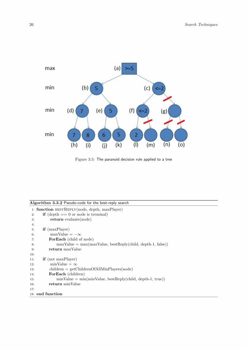
The paranoid decision rule (Sturtevant and Korf, 2000) reduces the game to a two-player game and thusthe αβ-framework can be applied. The root player assumes that all the opponents build a coalitionagainst him. The root player is the only max-player and all the other players are min-players whichtry to minimize the value of the root player. This is depicted in Figure 3.5. There, all the players inthe left subtree of Node (a) want to minimize the value and therefore the lowest value of this subtree ispropagated to the root node. After investigating the left subtree, the max-player knows that he will atleast get a value of 5. The first investigated leaf node of the right subtree has the value 2. The max-playerwill never play the move leading to this subtree and therefore all the other nodes of this subtree can bepruned. Beside this strength in pruning, the paranoid algorithm has one big weakness. Because of theunrealistic assumption that all opponent players form a coalition against the root player, suboptimal playcan occur (Sturtevant and Korf, 2000). The pseudo-code of the paranoid algorithm is exactly the sameas for the minimax algorithm (see Algorithm 3.1.1 and Algorithm A.1.1).
3.3.3 Best-Reply Search
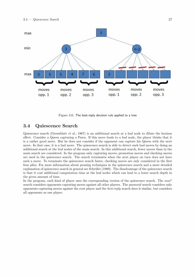
Best-reply search (Schadd and Winands, 2011) allows only the opponent with the strongest counter moveto play a move. The other opponents pass their move. Algorithm 3.3.2 presents the pseudo-code. Theunderlying assumption is that not all opponents try to minimize the value of the root player like theparanoid decision rule described in Subsection 3.3.2 does. The passing is one of the disadvantages ofthe algorithm because in some games it can lead to illegal positions. The advantage is that long-termplanning can be done compared to the other multi-player decision rules. This can be seen in Figure 3.6.The max-player is again on turn after one opponents move and so more max-nodes are visited. In thisfigure, there are three min-players, each of them has two legal moves in each position. The prunings inthe right subtree shows that αβ-pruning can be applied. Another advantage of this decision rule is thatthe playing style is less cautious compared to the paranoid decision rule (Schadd and Winands, 2011).At the same time, it has the disadvantage that opponent moves beneficial for the root player are notconsidered. The pseudo-code for the best-reply search with αβ-pruning is given in Algorithm A.3.1.
26 Search Techniques
Figure 3.5: The paranoid decision rule applied to a tree
Algorithm 3.3.2 Pseudo-code for the best-reply search
1: function bestReply(node, depth, maxPlayer)2: if (depth == 0 or node is terminal)3: return evaluate(node)4:
5: if (maxPlayer)6: maxValue = −∞7: ForEach (child of node)8: maxValue = max(maxValue, bestReply(child, depth-1, false))9: return maxValue
10:
11: if (not maxPlayer)12: minValue = ∞13: children = getChildrenOfAllMinPlayers(node)14: ForEach (children)15: minValue = min(minValue, bestReply(child, depth-1, true))16: return minValue17:
18: end function
3.4 — Quiescence Search 27
Figure 3.6: The best-reply decision rule applied to a tree
3.4 Quiescence Search
Quiescence search (Greenblatt et al., 1967) is an additional search at a leaf node to dilute the horizoneffect. Consider a Queen capturing a Pawn. If this move leads to a leaf node, the player thinks that itis a rather good move. But he does not consider if the opponent can capture his Queen with the nextmove. In that case, it is a bad move. The quiescence search is able to detect such bad moves by doing anadditional search at the leaf nodes of the main search. In this additional search, fewer moves than in themain search are considered. In the program only capturing moves, promotion moves and checking movesare used in the quiescence search. The search terminates when the next player on turn does not havesuch a move. To terminate the quiescence search faster, checking moves are only considered in the firstfour plies. For more information about pruning techniques in the quiescence search and a more detailedexplanation of quiescence search in general see Schrufer (1989). The disadvantage of the quiescence searchis that it cost additional computation time at the leaf nodes which can lead to a lower search depth inthe given amount of time.In the program, each kind of player uses the corresponding version of the quiescence search. The maxn
search considers opponents capturing moves against all other players. The paranoid search considers onlyopponents capturing moves against the root player and the best-reply search does it similar, but considersall opponents as one player.

28 Search Techniques
Chapter 4
Best-Reply Variants
In this chapter, first the weaknesses of best-reply are described in Section 4.1. Subsequently, ideas toovercome these weaknesses are presented in Section 4.2. The resulting search algorithms are described inSection 4.3. Section 4.4 gives an analysis of the complexity of the proposed algorithms and afterwards,the complexity of these algorithms in the domain of multi-player Chess is discussed in Section 4.4.6.
4.1 Weaknesses of the Best-Reply Search
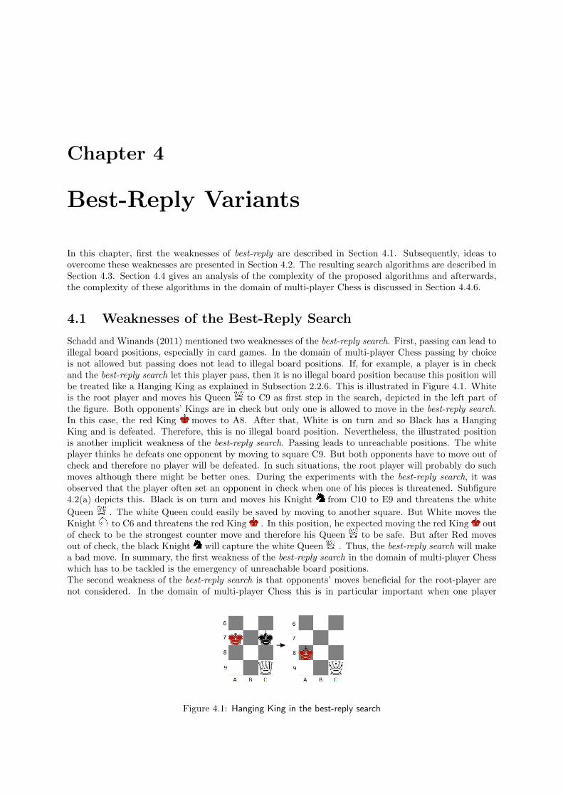
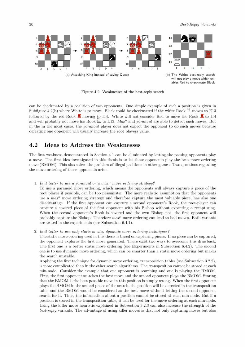
Schadd and Winands (2011) mentioned two weaknesses of the best-reply search. First, passing can lead toillegal board positions, especially in card games. In the domain of multi-player Chess passing by choiceis not allowed but passing does not lead to illegal board positions. If, for example, a player is in checkand the best-reply search let this player pass, then it is no illegal board position because this position willbe treated like a Hanging King as explained in Subsection 2.2.6. This is illustrated in Figure 4.1. Whiteis the root player and moves his Queen to C9 as first step in the search, depicted in the left part ofthe figure. Both opponents’ Kings are in check but only one is allowed to move in the best-reply search.In this case, the red King moves to A8. After that, White is on turn and so Black has a HangingKing and is defeated. Therefore, this is no illegal board position. Nevertheless, the illustrated positionis another implicit weakness of the best-reply search. Passing leads to unreachable positions. The whiteplayer thinks he defeats one opponent by moving to square C9. But both opponents have to move out ofcheck and therefore no player will be defeated. In such situations, the root player will probably do suchmoves although there might be better ones. During the experiments with the best-reply search, it wasobserved that the player often set an opponent in check when one of his pieces is threatened. Subfigure4.2(a) depicts this. Black is on turn and moves his Knight from C10 to E9 and threatens the white
Queen . The white Queen could easily be saved by moving to another square. But White moves theKnight to C6 and threatens the red King . In this position, he expected moving the red King outof check to be the strongest counter move and therefore his Queen to be safe. But after Red movesout of check, the black Knight will capture the white Queen . Thus, the best-reply search will makea bad move. In summary, the first weakness of the best-reply search in the domain of multi-player Chesswhich has to be tackled is the emergency of unreachable board positions.The second weakness of the best-reply search is that opponents’ moves beneficial for the root-player arenot considered. In the domain of multi-player Chess this is in particular important when one player
Figure 4.1: Hanging King in the best-reply search
30 Best-Reply Variants
(a) Attacking King instead of saving Queen (b) The White best-reply searchwill not play a move which en-ables Red to checkmate Black
Figure 4.2: Weaknesses of the best-reply search
can be checkmated by a coalition of two opponents. One simple example of such a position is given inSubfigure 4.2(b) where White is to move. Black could be checkmated if the white Rook moves to E13
followed by the red Rook moving to I14. White will not consider Red to move the Rook to I14and will probably not move his Rook to E13. Maxn and paranoid are able to detect such moves. Butin the in the most cases, the paranoid player does not expect the opponent to do such moves becausedefeating one opponent will usually increase the root players value.
4.2 Ideas to Address the Weaknesses
The first weakness demonstrated in Section 4.1 can be eliminated by letting the passing opponents playa move. The first idea investigated in this thesis is to let these opponents play the best move orderingmove (BMOM). This also solves the problem of illegal positions in other games. Two questions regardingthe move ordering of those opponents arise:
1. Is it better to use a paranoid or a maxn move ordering strategy?To use a paranoid move ordering, which means the opponents will always capture a piece of theroot player if possible, can be too pessimistic. The more realistic assumption that the opponentsuse a maxn move ordering strategy and therefore capture the most valuable piece, has also onedisadvantage. If the first opponent can capture a second opponent’s Rook, the root-player cancapture a covered piece of the first opponent with his Bishop without expecting a recapturing.When the second opponent’s Rook is covered and the own Bishop not, the first opponent willprobably capture the Bishop. Therefore maxn move ordering can lead to bad moves. Both variantsare tested in the experiments (see Subsection 6.4.1).
2. Is it better to use only static or also dynamic move ordering techniques?The static move ordering used in this thesis is based on capturing pieces. If no piece can be captured,the opponent explores the first move generated. There exist two ways to overcome this drawback.The first one is a better static move ordering (see Experiments in Subsection 6.4.2). The secondone is to use dynamic move ordering, which can be smarter than a static move ordering but makesthe search unstable.Applying the first technique for dynamic move ordering, transposition tables (see Subsection 3.2.2),is more complicated than in the other search algorithms. The transposition cannot be stored at eachmin-node. Consider the example that one opponent is searching and one is playing the BMOM.First, the first opponent searches the best move and the second opponent plays the BMOM. Storingthat the BMOM is the best possible move in this position is simply wrong. When the first opponentplays the BMOM in the second phase of the search, the position will be detected in the transpositiontable and the BMOM would be considered as the best move without letting the second opponentsearch for it. Thus, the information about a position cannot be stored at each min-node. But if aposition is stored in the transposition table, it can be used for the move ordering at each min-node.Using the killer move heuristic explained in Subsection 3.2.3 can also increase the strength of thebest-reply variants. The advantage of using killer moves is that not only capturing moves but also
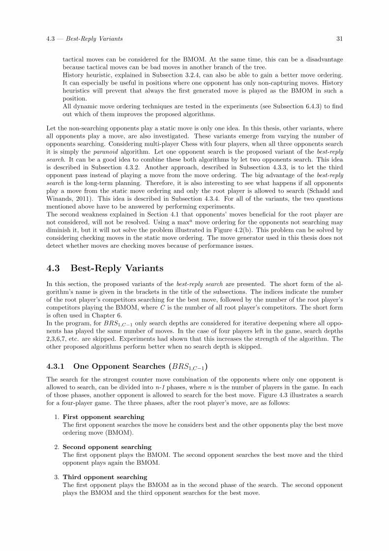
4.3 — Best-Reply Variants 31
tactical moves can be considered for the BMOM. At the same time, this can be a disadvantagebecause tactical moves can be bad moves in another branch of the tree.History heuristic, explained in Subsection 3.2.4, can also be able to gain a better move ordering.It can especially be useful in positions where one opponent has only non-capturing moves. Historyheuristics will prevent that always the first generated move is played as the BMOM in such aposition.All dynamic move ordering techniques are tested in the experiments (see Subsection 6.4.3) to findout which of them improves the proposed algorithms.
Let the non-searching opponents play a static move is only one idea. In this thesis, other variants, whereall opponents play a move, are also investigated. These variants emerge from varying the number ofopponents searching. Considering multi-player Chess with four players, when all three opponents searchit is simply the paranoid algorithm. Let one opponent search is the proposed variant of the best-replysearch. It can be a good idea to combine these both algorithms by let two opponents search. This ideais described in Subsection 4.3.2. Another approach, described in Subsection 4.3.3, is to let the thirdopponent pass instead of playing a move from the move ordering. The big advantage of the best-replysearch is the long-term planning. Therefore, it is also interesting to see what happens if all opponentsplay a move from the static move ordering and only the root player is allowed to search (Schadd andWinands, 2011). This idea is described in Subsection 4.3.4. For all of the variants, the two questionsmentioned above have to be answered by performing experiments.The second weakness explained in Section 4.1 that opponents’ moves beneficial for the root player arenot considered, will not be resolved. Using a maxn move ordering for the opponents not searching maydiminish it, but it will not solve the problem illustrated in Figure 4.2(b). This problem can be solved byconsidering checking moves in the static move ordering. The move generator used in this thesis does notdetect whether moves are checking moves because of performance issues.
4.3 Best-Reply Variants
In this section, the proposed variants of the best-reply search are presented. The short form of the al-gorithm’s name is given in the brackets in the title of the subsections. The indices indicate the numberof the root player’s competitors searching for the best move, followed by the number of the root player’scompetitors playing the BMOM, where C is the number of all root player’s competitors. The short formis often used in Chapter 6.In the program, for BRS1,C−1 only search depths are considered for iterative deepening where all oppo-nents has played the same number of moves. In the case of four players left in the game, search depths2,3,6,7, etc. are skipped. Experiments had shown that this increases the strength of the algorithm. Theother proposed algorithms perform better when no search depth is skipped.
4.3.1 One Opponent Searches (BRS1,C−1)
The search for the strongest counter move combination of the opponents where only one opponent isallowed to search, can be divided into n-1 phases, where n is the number of players in the game. In eachof those phases, another opponent is allowed to search for the best move. Figure 4.3 illustrates a searchfor a four-player game. The three phases, after the root player’s move, are as follows:
1. First opponent searchingThe first opponent searches the move he considers best and the other opponents play the best moveordering move (BMOM).
2. Second opponent searchingThe first opponent plays the BMOM. The second opponent searches the best move and the thirdopponent plays again the BMOM.
3. Third opponent searchingThe first opponent plays the BMOM as in the second phase of the search. The second opponentplays the BMOM and the third opponent searches for the best move.
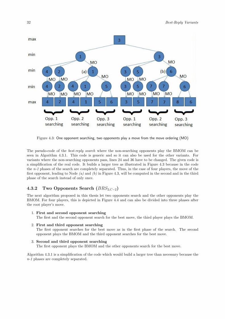
32 Best-Reply Variants
Figure 4.3: One opponent searching, two opponents play a move from the move ordering (MO)
The pseudo-code of the best-reply search where the non-searching opponents play the BMOM can beseen in Algorithm 4.3.1. This code is generic and so it can also be used for the other variants. Forvariants where the non-searching opponents pass, lines 24 and 36 have to be changed. The given code isa simplification of the real code. It builds a larger tree as illustrated in Figure 4.3 because in the codethe n-1 phases of the search are completely separated. Thus, in the case of four players, the move of thefirst opponent, leading to Node (a) and (b) in Figure 4.3, will be computed in the second and in the thirdphase of the search instead of only once.
4.3.2 Two Opponents Search (BRS2,C−2)
The next algorithm proposed in this thesis let two opponents search and the other opponents play theBMOM. For four players, this is depicted in Figure 4.4 and can also be divided into three phases afterthe root player’s move.
1. First and second opponent searchingThe first and the second opponent search for the best move, the third player plays the BMOM.
2. First and third opponent searchingThe first opponent searches for the best move as in the first phase of the search. The secondopponent plays the BMOM and the third opponent searches for the best move.
3. Second and third opponent searchingThe first opponent plays the BMOM and the other opponents search for the best move.
Algorithm 4.3.1 is a simplification of the code which would build a larger tree than necessary because then-1 phases are completely separated.
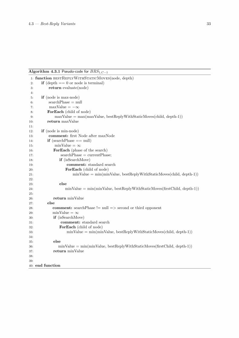
4.3 — Best-Reply Variants 33
Algorithm 4.3.1 Pseudo-code for BRS1,C−1
1: function bestReplyWithStaticMoves(node, depth)2: if (depth == 0 or node is terminal)3: return evaluate(node)4:
5: if (node is max-node)6: searchPhase = null7: maxValue = −∞8: ForEach (child of node)9: maxValue = max(maxValue, bestReplyWithStaticMoves(child, depth-1))
10: return maxValue11:
12: if (node is min-node)13: comment: first Node after maxNode14: if (searchPhase == null)15: minValue = ∞16: ForEach (phase of the search)17: searchPhase = currentPhase;18: if (isSearchMove)19: comment: standard search20: ForEach (child of node)21: minValue = min(minValue, bestReplyWithStaticMoves(child, depth-1))22:
23: else24: minValue = min(minValue, bestReplyWithStaticMoves(firstChild, depth-1))25:
26: return minValue27: else28: comment: searchPhase != null => second or third opponent29: minValue = ∞30: if (isSearchMove)31: comment: standard search32: ForEach (child of node)33: minValue = min(minValue, bestReplyWithStaticMoves(child, depth-1))34:
35: else36: minValue = min(minValue, bestReplyWithStaticMoves(firstChild, depth-1))37: return minValue38:
39:
40: end function
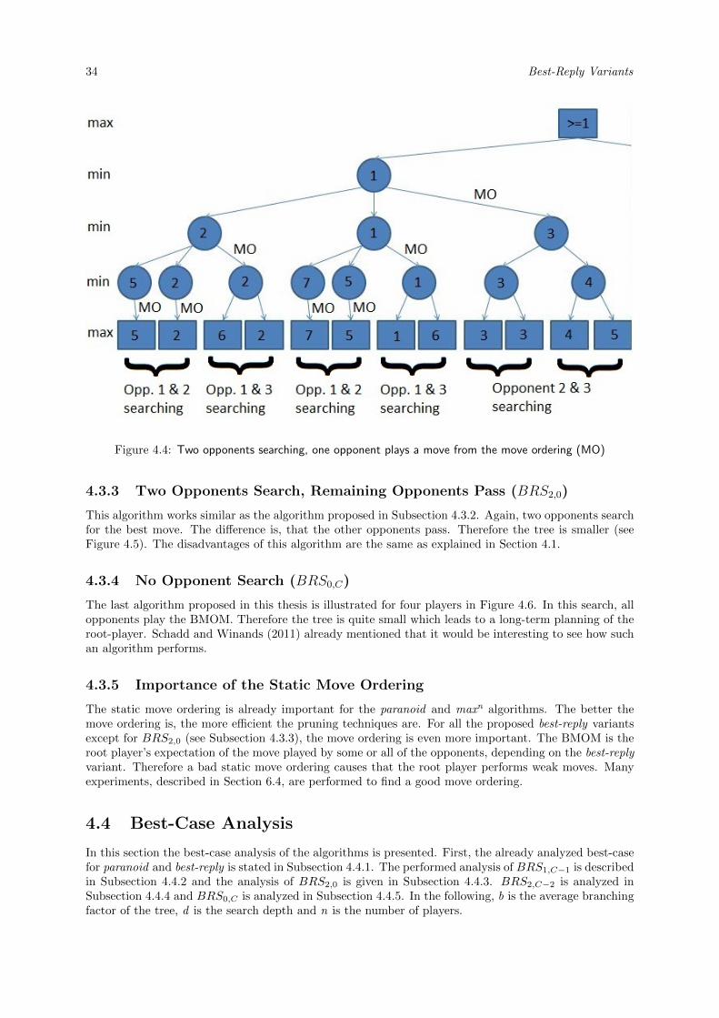
34 Best-Reply Variants
Figure 4.4: Two opponents searching, one opponent plays a move from the move ordering (MO)
4.3.3 Two Opponents Search, Remaining Opponents Pass (BRS2,0)
This algorithm works similar as the algorithm proposed in Subsection 4.3.2. Again, two opponents searchfor the best move. The difference is, that the other opponents pass. Therefore the tree is smaller (seeFigure 4.5). The disadvantages of this algorithm are the same as explained in Section 4.1.
4.3.4 No Opponent Search (BRS0,C)
The last algorithm proposed in this thesis is illustrated for four players in Figure 4.6. In this search, allopponents play the BMOM. Therefore the tree is quite small which leads to a long-term planning of theroot-player. Schadd and Winands (2011) already mentioned that it would be interesting to see how suchan algorithm performs.
4.3.5 Importance of the Static Move Ordering
The static move ordering is already important for the paranoid and maxn algorithms. The better themove ordering is, the more efficient the pruning techniques are. For all the proposed best-reply variantsexcept for BRS2,0 (see Subsection 4.3.3), the move ordering is even more important. The BMOM is theroot player’s expectation of the move played by some or all of the opponents, depending on the best-replyvariant. Therefore a bad static move ordering causes that the root player performs weak moves. Manyexperiments, described in Section 6.4, are performed to find a good move ordering.
4.4 Best-Case Analysis
In this section the best-case analysis of the algorithms is presented. First, the already analyzed best-casefor paranoid and best-reply is stated in Subsection 4.4.1. The performed analysis of BRS1,C−1 is describedin Subsection 4.4.2 and the analysis of BRS2,0 is given in Subsection 4.4.3. BRS2,C−2 is analyzed inSubsection 4.4.4 and BRS0,C is analyzed in Subsection 4.4.5. In the following, b is the average branchingfactor of the tree, d is the search depth and n is the number of players.
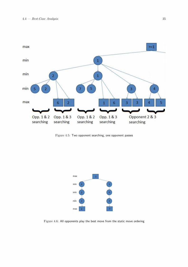
4.4 — Best-Case Analysis 35
Figure 4.5: Two opponent searching, one opponent passes
Figure 4.6: All opponents play the best move from the static move ordering
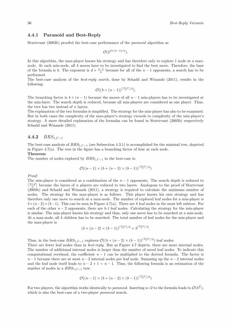
36 Best-Reply Variants
4.4.1 Paranoid and Best-Reply
Sturtevant (2003b) proofed the best-case performance of the paranoid algorithm as
O(bd×(n−1)/n).
In this algorithm, the max-player knows his strategy and has therefore only to explore 1 node at a max-node. At each min-node, all b moves have to be investigated to find the best move. Therefore, the baseof the formula is b. The exponent is d × n−1
n because for all of the n − 1 opponents, a search has to beperformed.The best-case analysis of the best-reply search, done by Schadd and Winands (2011), results in thefollowing:
O((b× (n− 1))d2×dn e/2).
The branching factor is b× (n− 1) because the moves of all n− 1 min-players has to be investigated atthe min-layer. The search depth is reduced, because all min-players are considered as one player. Thus,the tree has two instead of n layers.The explanation of the two formulas is simplified. The strategy for the min-player has also to be examined.But in both cases the complexity of the max-player’s strategy exceeds to complexity of the min-player’sstrategy. A more detailed explanation of the formulas can be found in Sturtevant (2003b) respectivelySchadd and Winands (2011).
4.4.2 BRS1,C−1
The best-case analysis of BRS1,C−1 (see Subsection 4.3.1) is accomplished for the minimal tree, depictedin Figure 4.7(a). The tree in the figure has a branching factor of four at each node.Theorem:The number of nodes explored by BRS1,C−1 in the best-case is:
O((n− 1)× (b + (n− 2)× (b− 1))d2×dn e/2)
Proof:The min-player is considered as a combination of the n − 1 opponents. The search depth is reduced tod 2×dn e because the layers of n players are reduced to two layers. Analogous to the proof of Sturtevant(2003b) and Schadd and Winands (2011), a strategy is required to calculate the minimum number ofnodes. The strategy for the max-player is as follows. This player knows his own strategy and hastherefore only one move to search at a max-node. The number of explored leaf nodes for a min-player isb+(n−2)×(b−1). This can be seen in Figure 4.7(a). There are b leaf nodes in the most left subtree. Foreach of the other n − 2 opponents, there are b-1 leaf nodes. Calculating the strategy for the min-playeris similar. The min-player knows his strategy and thus, only one move has to be searched at a min-node.At a max-node, all b children has to be searched. The total number of leaf nodes for the min-player andthe max-player is
(b + (n− 2)× (b− 1))d2×dn e/2 + bd
2×dn e/2.
Thus, in the best-case BRS1,C−1 explores O((b + (n− 2)× (b− 1))d2×dn e/2) leaf nodes.
There are fewer leaf nodes than in best-reply. But as Figure 4.7 depicts, there are more internal nodes.The number of additional internal nodes is larger than the number of saved leaf nodes. To indicate thiscomputational overhead, the coefficient n − 1 can be multiplied to the derived formula. The factor isn− 1 because there are at most n− 2 internal nodes per leaf node. Summing up the n− 2 internal nodesand the leaf node itself leads to n − 2 + 1 = n − 1. Thus, the following formula is an estimation of thenumber of nodes in a BRS1,C−1 tree.
O((n− 1)× (b + (n− 2)× (b− 1))d2×dn e/2)
For two players, the algorithm works identically to paranoid. Inserting n=2 to the formula leads to O(bd2 ),
which is also the best-case of a two-player paranoid search.
4.4 — Best-Case Analysis 37
(a) Nodes in a BRS1,C−1 tree (b) Nodes in a BRS tree
Figure 4.7: Comparison of a BRS1,C−1 and a BRS tree
4.4.3 BRS2,0
The best-case analysis for BRS2,0, described in Subsection 4.3.3, is quite easy.Theorem:The number of nodes explored by BRS2,0 in the best-case is:
O(BRS2,0(b, d,n)) =
O(( b2×(n−1)×(n−2)2 )d
2×dn e/2), if n > 3
O(bd×(n−1)/n), if n ≤ 3
Proof:For two and three players, the algorithm works exactly as paranoid. Therefore the best-case analysisfrom paranoid can be used for n ≤ 3. To calculate the number of nodes for more than 3 players, allthe min-players are considered as one player and therefore the exponent is d 2×dn e. The strategy for themin-player is the same as for BRS1,C−1. The min-player knows his strategy and has therefore only toexamine one node at a min-node. At a max-node, b nodes have to be explored. Again, the strategyof the min-player is not important to calculate the complexity because the strategy of the max-playeris much more complex. The max-player has to explore 1 node at a max-node. At a min-node, thecalculation of the number of paths leading to leaf nodes is the well-known urn problem (Johnson andKotz, 1977; Papula, 2001). 2 out of the n − 1 opponents play a move, the other opponents pass. Theorder does not matter. For instance, Opponent 1 playing a move followed by Opponent 3 playing themove is considered as the same as Opponent 3 playing a move followed by Opponent 1 playing a movebecause only the first way is allowed in the proposed algorithm. Therefore,(
n− 1
2
)=
(n− 1)!
2!× (n− 3)!=
(n− 1)× (n− 2)
2
paths lead to leaf nodes. Each path leads to b2 leaf nodes. There are much fewer internal nodes thanleaf nodes. Thus, they can be neglected. In conclusion, the number of nodes in BRS2,0 for more than 3players are:
O((b2 × (n− 1)× (n− 2)
2)d
2×dn e/2)
4.4.4 BRS2,C−2
In this subsection, the best-case analysis of BRS2,C−2, explained in Subsection 4.3.2, is given.Theorem:The number of nodes explored by BRS2,C−2 in the best-case is:
O(BRS2,C−2(b, d,n)) =
O((n− 2)× ( b2×(n−1)×(n−2)2 )d
2×dn e/2), if n > 3
O(bd×(n−1)/n), if n ≤ 3
Proof:The formula to calculate the number of nodes for BRS2,C−2 is similar to the formula for BRS2,0. Thenumber of leaf nodes are exactly the same. But BRS2,C−2 has more internal nodes. To indicate thiscomputational overhead, n− 2 can be multiplied to the number of leaf nodes.
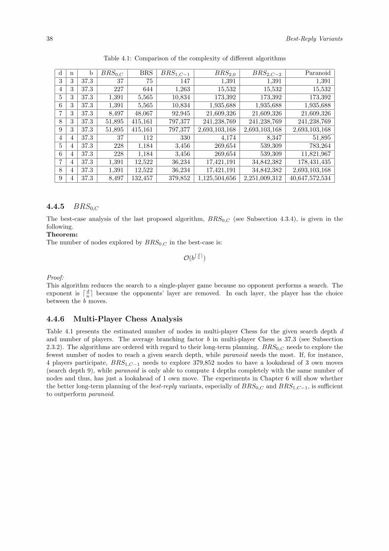
38 Best-Reply Variants
Table 4.1: Comparison of the complexity of different algorithms
d n b BRS0,C BRS BRS1,C−1 BRS2,0 BRS2,C−2 Paranoid3 3 37.3 37 75 147 1,391 1,391 1,3914 3 37.3 227 644 1,263 15,532 15,532 15,5325 3 37.3 1,391 5,565 10,834 173,392 173,392 173,3926 3 37.3 1,391 5,565 10,834 1,935,688 1,935,688 1,935,6887 3 37.3 8,497 48,067 92,945 21,609,326 21,609,326 21,609,3268 3 37.3 51,895 415,161 797,377 241,238,769 241,238,769 241,238,7699 3 37.3 51,895 415,161 797,377 2,693,103,168 2,693,103,168 2,693,103,1684 4 37.3 37 112 330 4,174 8,347 51,8955 4 37.3 228 1,184 3,456 269,654 539,309 783,2646 4 37.3 228 1,184 3,456 269,654 539,309 11,821,9677 4 37.3 1,391 12,522 36,234 17,421,191 34,842,382 178,431,4358 4 37.3 1,391 12,522 36,234 17,421,191 34,842,382 2,693,103,1689 4 37.3 8,497 132,457 379,852 1,125,504,656 2,251,009,312 40,647,572,534
4.4.5 BRS0,C
The best-case analysis of the last proposed algorithm, BRS0,C (see Subsection 4.3.4), is given in thefollowing.Theorem:The number of nodes explored by BRS0,C in the best-case is:
O(bddn e)
Proof:This algorithm reduces the search to a single-player game because no opponent performs a search. Theexponent is d dne because the opponents’ layer are removed. In each layer, the player has the choicebetween the b moves.
4.4.6 Multi-Player Chess Analysis
Table 4.1 presents the estimated number of nodes in multi-player Chess for the given search depth dand number of players. The average branching factor b in multi-player Chess is 37.3 (see Subsection2.3.2). The algorithms are ordered with regard to their long-term planning. BRS0,C needs to explore thefewest number of nodes to reach a given search depth, while paranoid needs the most. If, for instance,4 players participate, BRS1,C−1 needs to explore 379,852 nodes to have a lookahead of 3 own moves(search depth 9), while paranoid is only able to compute 4 depths completely with the same number ofnodes and thus, has just a lookahead of 1 own move. The experiments in Chapter 6 will show whetherthe better long-term planning of the best-reply variants, especially of BRS0,C and BRS1,C−1, is sufficientto outperform paranoid.
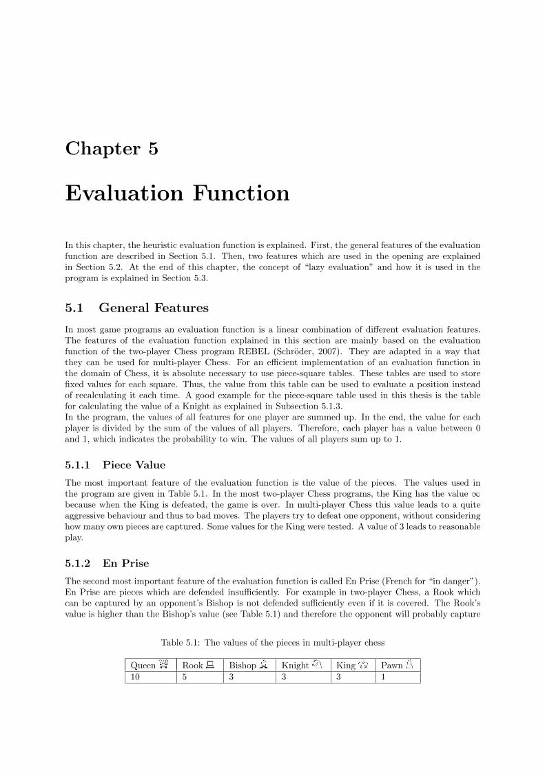
Chapter 5
Evaluation Function
In this chapter, the heuristic evaluation function is explained. First, the general features of the evaluationfunction are described in Section 5.1. Then, two features which are used in the opening are explainedin Section 5.2. At the end of this chapter, the concept of “lazy evaluation” and how it is used in theprogram is explained in Section 5.3.
5.1 General Features
In most game programs an evaluation function is a linear combination of different evaluation features.The features of the evaluation function explained in this section are mainly based on the evaluationfunction of the two-player Chess program REBEL (Schroder, 2007). They are adapted in a way thatthey can be used for multi-player Chess. For an efficient implementation of an evaluation function inthe domain of Chess, it is absolute necessary to use piece-square tables. These tables are used to storefixed values for each square. Thus, the value from this table can be used to evaluate a position insteadof recalculating it each time. A good example for the piece-square table used in this thesis is the tablefor calculating the value of a Knight as explained in Subsection 5.1.3.In the program, the values of all features for one player are summed up. In the end, the value for eachplayer is divided by the sum of the values of all players. Therefore, each player has a value between 0and 1, which indicates the probability to win. The values of all players sum up to 1.
5.1.1 Piece Value
The most important feature of the evaluation function is the value of the pieces. The values used inthe program are given in Table 5.1. In the most two-player Chess programs, the King has the value ∞because when the King is defeated, the game is over. In multi-player Chess this value leads to a quiteaggressive behaviour and thus to bad moves. The players try to defeat one opponent, without consideringhow many own pieces are captured. Some values for the King were tested. A value of 3 leads to reasonableplay.
5.1.2 En Prise
The second most important feature of the evaluation function is called En Prise (French for “in danger”).En Prise are pieces which are defended insufficiently. For example in two-player Chess, a Rook whichcan be captured by an opponent’s Bishop is not defended sufficiently even if it is covered. The Rook’svalue is higher than the Bishop’s value (see Table 5.1) and therefore the opponent will probably capture
Table 5.1: The values of the pieces in multi-player chess
Queen Rook Bishop Knight King Pawn10 5 3 3 3 1
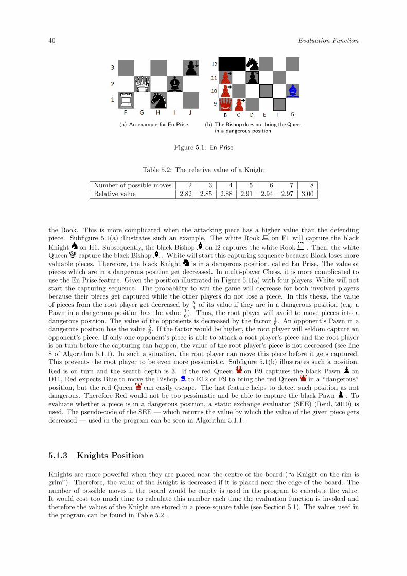
40 Evaluation Function
(a) An example for En Prise (b) The Bishop does not bring the Queenin a dangerous position
Figure 5.1: En Prise
Table 5.2: The relative value of a Knight
Number of possible moves 2 3 4 5 6 7 8Relative value 2.82 2.85 2.88 2.91 2.94 2.97 3.00
the Rook. This is more complicated when the attacking piece has a higher value than the defendingpiece. Subfigure 5.1(a) illustrates such an example. The white Rook on F1 will capture the black
Knight on H1. Subsequently, the black Bishop on I2 captures the white Rook . Then, the whiteQueen capture the black Bishop . White will start this capturing sequence because Black loses morevaluable pieces. Therefore, the black Knight is in a dangerous position, called En Prise. The value ofpieces which are in a dangerous position get decreased. In multi-player Chess, it is more complicated touse the En Prise feature. Given the position illustrated in Figure 5.1(a) with four players, White will notstart the capturing sequence. The probability to win the game will decrease for both involved playersbecause their pieces get captured while the other players do not lose a piece. In this thesis, the valueof pieces from the root player get decreased by 5
6 of its value if they are in a dangerous position (e.g, aPawn in a dangerous position has the value 1
6 ). Thus, the root player will avoid to move pieces into adangerous position. The value of the opponents is decreased by the factor 1
6 . An opponent’s Pawn in adangerous position has the value 5
6 . If the factor would be higher, the root player will seldom capture anopponent’s piece. If only one opponent’s piece is able to attack a root player’s piece and the root playeris on turn before the capturing can happen, the value of the root player’s piece is not decreased (see line8 of Algorithm 5.1.1). In such a situation, the root player can move this piece before it gets captured.This prevents the root player to be even more pessimistic. Subfigure 5.1(b) illustrates such a position.
Red is on turn and the search depth is 3. If the red Queen on B9 captures the black Pawn onD11, Red expects Blue to move the Bishop to E12 or F9 to bring the red Queen in a “dangerous”position, but the red Queen can easily escape. The last feature helps to detect such position as notdangerous. Therefore Red would not be too pessimistic and be able to capture the black Pawn . Toevaluate whether a piece is in a dangerous position, a static exchange evaluator (SEE) (Reul, 2010) isused. The pseudo-code of the SEE — which returns the value by which the value of the given piece getsdecreased — used in the program can be seen in Algorithm 5.1.1.
5.1.3 Knights Position
Knights are more powerful when they are placed near the centre of the board (“a Knight on the rim isgrim”). Therefore, the value of the Knight is decreased if it is placed near the edge of the board. Thenumber of possible moves if the board would be empty is used in the program to calculate the value.It would cost too much time to calculate this number each time the evaluation function is invoked andtherefore the values of the Knight are stored in a piece-square table (see Section 5.1). The values used inthe program can be found in Table 5.2.
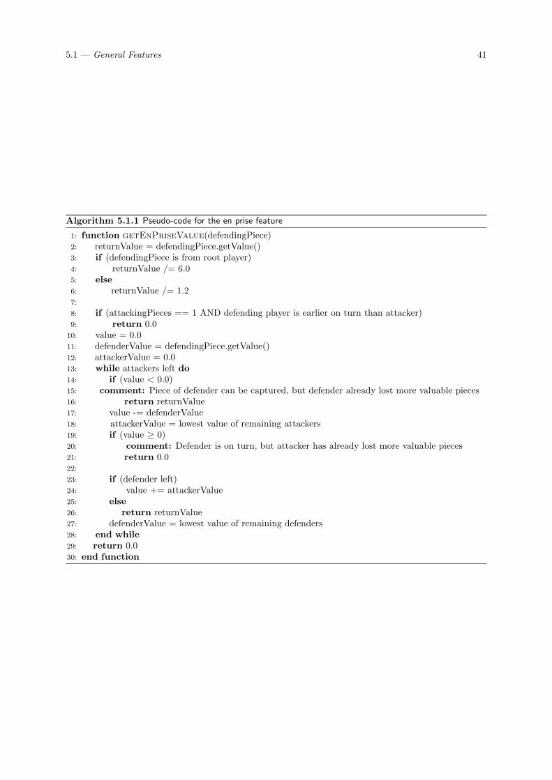
5.1 — General Features 41
Algorithm 5.1.1 Pseudo-code for the en prise feature
1: function getEnPriseValue(defendingPiece)2: returnValue = defendingPiece.getValue()3: if (defendingPiece is from root player)4: returnValue /= 6.05: else6: returnValue /= 1.27:
8: if (attackingPieces == 1 AND defending player is earlier on turn than attacker)9: return 0.0
10: value = 0.011: defenderValue = defendingPiece.getValue()12: attackerValue = 0.013: while attackers left do14: if (value < 0.0)15: comment: Piece of defender can be captured, but defender already lost more valuable pieces16: return returnValue17: value -= defenderValue18: attackerValue = lowest value of remaining attackers19: if (value ≥ 0)20: comment: Defender is on turn, but attacker has already lost more valuable pieces21: return 0.022:
23: if (defender left)24: value += attackerValue25: else26: return returnValue27: defenderValue = lowest value of remaining defenders28: end while29: return 0.030: end function
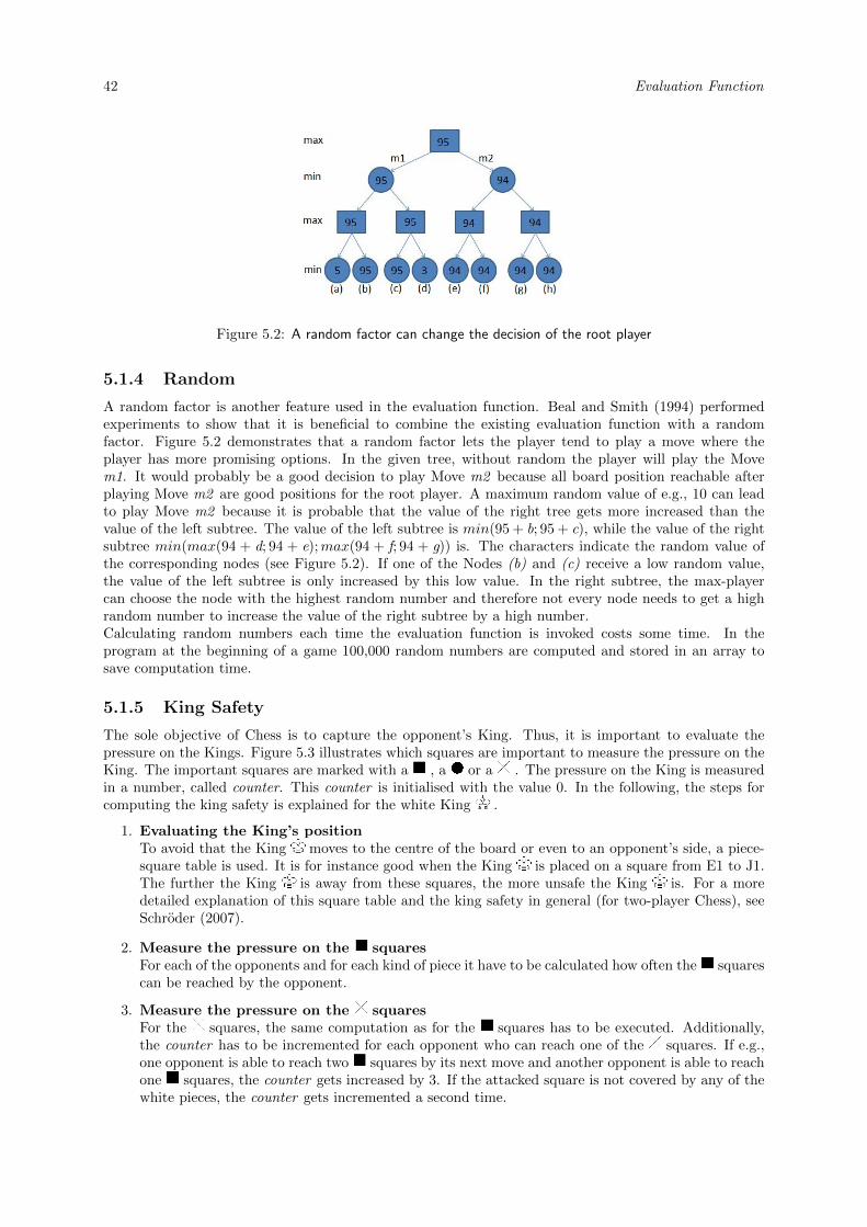
42 Evaluation Function
Figure 5.2: A random factor can change the decision of the root player
5.1.4 Random
A random factor is another feature used in the evaluation function. Beal and Smith (1994) performedexperiments to show that it is beneficial to combine the existing evaluation function with a randomfactor. Figure 5.2 demonstrates that a random factor lets the player tend to play a move where theplayer has more promising options. In the given tree, without random the player will play the Movem1. It would probably be a good decision to play Move m2 because all board position reachable afterplaying Move m2 are good positions for the root player. A maximum random value of e.g., 10 can leadto play Move m2 because it is probable that the value of the right tree gets more increased than thevalue of the left subtree. The value of the left subtree is min(95 + b; 95 + c), while the value of the rightsubtree min(max(94 + d; 94 + e);max(94 + f; 94 + g)) is. The characters indicate the random value ofthe corresponding nodes (see Figure 5.2). If one of the Nodes (b) and (c) receive a low random value,the value of the left subtree is only increased by this low value. In the right subtree, the max-playercan choose the node with the highest random number and therefore not every node needs to get a highrandom number to increase the value of the right subtree by a high number.Calculating random numbers each time the evaluation function is invoked costs some time. In theprogram at the beginning of a game 100,000 random numbers are computed and stored in an array tosave computation time.
5.1.5 King Safety
The sole objective of Chess is to capture the opponent’s King. Thus, it is important to evaluate thepressure on the Kings. Figure 5.3 illustrates which squares are important to measure the pressure on theKing. The important squares are marked with a , a or a . The pressure on the King is measuredin a number, called counter. This counter is initialised with the value 0. In the following, the steps forcomputing the king safety is explained for the white King .
1. Evaluating the King’s positionTo avoid that the King moves to the centre of the board or even to an opponent’s side, a piece-square table is used. It is for instance good when the King is placed on a square from E1 to J1.The further the King is away from these squares, the more unsafe the King is. For a moredetailed explanation of this square table and the king safety in general (for two-player Chess), seeSchroder (2007).
2. Measure the pressure on the squaresFor each of the opponents and for each kind of piece it have to be calculated how often the squarescan be reached by the opponent.
3. Measure the pressure on the squaresFor the squares, the same computation as for the squares has to be executed. Additionally,the counter has to be incremented for each opponent who can reach one of the squares. If e.g.,one opponent is able to reach two squares by its next move and another opponent is able to reachone squares, the counter gets increased by 3. If the attacked square is not covered by any of thewhite pieces, the counter gets incremented a second time.
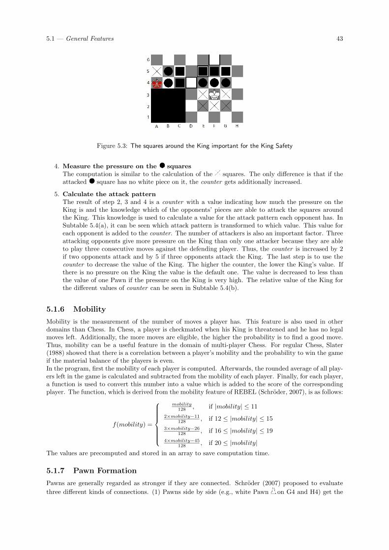
5.1 — General Features 43
Figure 5.3: The squares around the King important for the King Safety
4. Measure the pressure on the squaresThe computation is similar to the calculation of the squares. The only difference is that if theattacked square has no white piece on it, the counter gets additionally increased.
5. Calculate the attack patternThe result of step 2, 3 and 4 is a counter with a value indicating how much the pressure on theKing is and the knowledge which of the opponents’ pieces are able to attack the squares aroundthe King. This knowledge is used to calculate a value for the attack pattern each opponent has. InSubtable 5.4(a), it can be seen which attack pattern is transformed to which value. This value foreach opponent is added to the counter. The number of attackers is also an important factor. Threeattacking opponents give more pressure on the King than only one attacker because they are ableto play three consecutive moves against the defending player. Thus, the counter is increased by 2if two opponents attack and by 5 if three opponents attack the King. The last step is to use thecounter to decrease the value of the King. The higher the counter, the lower the King’s value. Ifthere is no pressure on the King the value is the default one. The value is decreased to less thanthe value of one Pawn if the pressure on the King is very high. The relative value of the King forthe different values of counter can be seen in Subtable 5.4(b).
5.1.6 Mobility
Mobility is the measurement of the number of moves a player has. This feature is also used in otherdomains than Chess. In Chess, a player is checkmated when his King is threatened and he has no legalmoves left. Additionally, the more moves are eligible, the higher the probability is to find a good move.Thus, mobility can be a useful feature in the domain of multi-player Chess. For regular Chess, Slater(1988) showed that there is a correlation between a player’s mobility and the probability to win the gameif the material balance of the players is even.In the program, first the mobility of each player is computed. Afterwards, the rounded average of all play-ers left in the game is calculated and subtracted from the mobility of each player. Finally, for each player,a function is used to convert this number into a value which is added to the score of the correspondingplayer. The function, which is derived from the mobility feature of REBEL (Schroder, 2007), is as follows:
f(mobility) =
mobility128 , if |mobility| ≤ 11
2×mobility−11128 , if 12 ≤ |mobility| ≤ 15
3×mobility−26128 , if 16 ≤ |mobility| ≤ 19
4×mobility−45128 , if 20 ≤ |mobility|
The values are precomputed and stored in an array to save computation time.
5.1.7 Pawn Formation
Pawns are generally regarded as stronger if they are connected. Schroder (2007) proposed to evaluate
three different kinds of connections. (1) Pawns side by side (e.g., white Pawn on G4 and H4) get the
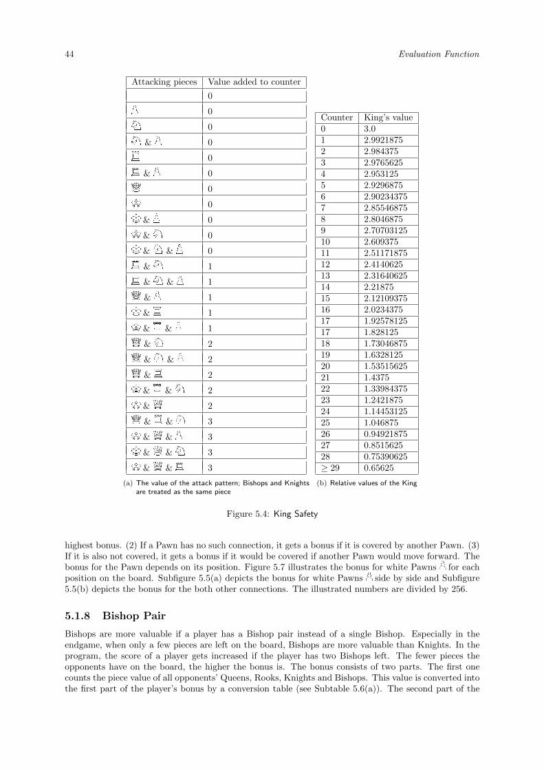
44 Evaluation Function
Attacking pieces Value added to counter
0
0
0
& 0
0
& 0
0
0
& 0
& 0
& & 0
& 1
& & 1
& 1
& 1
& & 1
& 2
& & 2
& 2
& & 2
& 2
& & 3
& & 3
& & 3
& & 3
(a) The value of the attack pattern; Bishops and Knightsare treated as the same piece
Counter King’s value0 3.01 2.99218752 2.9843753 2.97656254 2.9531255 2.92968756 2.902343757 2.855468758 2.80468759 2.7070312510 2.60937511 2.5117187512 2.414062513 2.3164062514 2.2187515 2.1210937516 2.023437517 1.9257812517 1.82812518 1.7304687519 1.632812520 1.5351562521 1.437522 1.3398437523 1.242187524 1.1445312525 1.04687526 0.9492187527 0.851562528 0.75390625≥ 29 0.65625
(b) Relative values of the King
Figure 5.4: King Safety
highest bonus. (2) If a Pawn has no such connection, it gets a bonus if it is covered by another Pawn. (3)If it is also not covered, it gets a bonus if it would be covered if another Pawn would move forward. Thebonus for the Pawn depends on its position. Figure 5.7 illustrates the bonus for white Pawns for eachposition on the board. Subfigure 5.5(a) depicts the bonus for white Pawns side by side and Subfigure5.5(b) depicts the bonus for the both other connections. The illustrated numbers are divided by 256.
5.1.8 Bishop Pair
Bishops are more valuable if a player has a Bishop pair instead of a single Bishop. Especially in theendgame, when only a few pieces are left on the board, Bishops are more valuable than Knights. In theprogram, the score of a player gets increased if the player has two Bishops left. The fewer pieces theopponents have on the board, the higher the bonus is. The bonus consists of two parts. The first onecounts the piece value of all opponents’ Queens, Rooks, Knights and Bishops. This value is converted intothe first part of the player’s bonus by a conversion table (see Subtable 5.6(a)). The second part of the
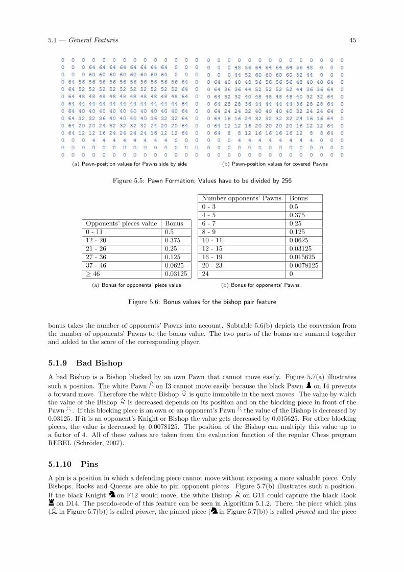
5.1 — General Features 45
(a) Pawn-position values for Pawns side by side (b) Pawn-position values for covered Pawns
Figure 5.5: Pawn Formation; Values have to be divided by 256
Opponents’ pieces value Bonus0 - 11 0.512 - 20 0.37521 - 26 0.2527 - 36 0.12537 - 46 0.0625≥ 46 0.03125
(a) Bonus for opponents’ piece value
Number opponents’ Pawns Bonus0 - 3 0.54 - 5 0.3756 - 7 0.258 - 9 0.12510 - 11 0.062512 - 15 0.0312516 - 19 0.01562520 - 23 0.007812524 0
(b) Bonus for opponents’ Pawns
Figure 5.6: Bonus values for the bishop pair feature
bonus takes the number of opponents’ Pawns into account. Subtable 5.6(b) depicts the conversion fromthe number of opponents’ Pawns to the bonus value. The two parts of the bonus are summed togetherand added to the score of the corresponding player.
5.1.9 Bad Bishop
A bad Bishop is a Bishop blocked by an own Pawn that cannot move easily. Figure 5.7(a) illustrates
such a position. The white Pawn on I3 cannot move easily because the black Pawn on I4 preventsa forward move. Therefore the white Bishop is quite immobile in the next moves. The value by whichthe value of the Bishop is decreased depends on its position and on the blocking piece in front of thePawn . If this blocking piece is an own or an opponent’s Pawn the value of the Bishop is decreased by0.03125. If it is an opponent’s Knight or Bishop the value gets decreased by 0.015625. For other blockingpieces, the value is decreased by 0.0078125. The position of the Bishop can multiply this value up toa factor of 4. All of these values are taken from the evaluation function of the regular Chess programREBEL (Schroder, 2007).
5.1.10 Pins
A pin is a position in which a defending piece cannot move without exposing a more valuable piece. OnlyBishops, Rooks and Queens are able to pin opponent pieces. Figure 5.7(b) illustrates such a position.
If the black Knight on F12 would move, the white Bishop on G11 could capture the black Rookon D14. The pseudo-code of this feature can be seen in Algorithm 5.1.2. There, the piece which pins
( in Figure 5.7(b)) is called pinner, the pinned piece ( in Figure 5.7(b)) is called pinned and the piece
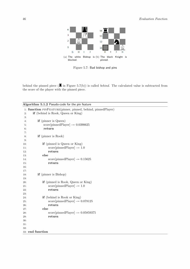
46 Evaluation Function
(a) The white Bishop isblocked.
(b) The black Knight ispinned.
Figure 5.7: Bad bishop and pins
behind the pinned piece ( in Figure 5.7(b)) is called behind. The calculated value is subtracted fromthe score of the player with the pinned piece.
Algorithm 5.1.2 Pseudo-code for the pin feature
1: function pinFeature(pinner, pinned, behind, pinnedPlayer)2: if (behind is Rook, Queen or King)3:
4: if (pinner is Queen)5: score[pinnedPlayer] -= 0.03906256: return7:
8: if (pinner is Rook)9:
10: if (pinned is Queen or King)11: score[pinnedPlayer] -= 1.012: return13: else14: score[pinnedPlayer] -= 0.1562515: return16:
17:
18: if (pinner is Bishop)19:
20: if (pinned is Rook, Queen or King)21: score[pinnedPlayer] -= 1.022: return23:
24: if (behind is Rook or King)25: score[pinnedPlayer] -= 0.07812526: return27: else28: score[pinnedPlayer] -= 0.0585937529: return30:
31:
32:
33: end function
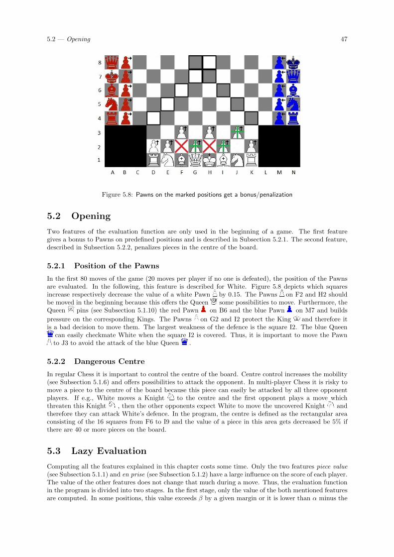
5.2 — Opening 47
Figure 5.8: Pawns on the marked positions get a bonus/penalization
5.2 Opening
Two features of the evaluation function are only used in the beginning of a game. The first featuregives a bonus to Pawns on predefined positions and is described in Subsection 5.2.1. The second feature,described in Subsection 5.2.2, penalizes pieces in the centre of the board.
5.2.1 Position of the Pawns
In the first 80 moves of the game (20 moves per player if no one is defeated), the position of the Pawnsare evaluated. In the following, this feature is described for White. Figure 5.8 depicts which squaresincrease respectively decrease the value of a white Pawn by 0.15. The Pawns on F2 and H2 shouldbe moved in the beginning because this offers the Queen some possibilities to move. Furthermore, theQueen pins (see Subsection 5.1.10) the red Pawn on B6 and the blue Pawn on M7 and builds
pressure on the corresponding Kings. The Pawns on G2 and I2 protect the King and therefore itis a bad decision to move them. The largest weakness of the defence is the square I2. The blue Queen
can easily checkmate White when the square I2 is covered. Thus, it is important to move the Pawnto J3 to avoid the attack of the blue Queen .
5.2.2 Dangerous Centre
In regular Chess it is important to control the centre of the board. Centre control increases the mobility(see Subsection 5.1.6) and offers possibilities to attack the opponent. In multi-player Chess it is risky tomove a piece to the centre of the board because this piece can easily be attacked by all three opponentplayers. If e.g., White moves a Knight to the centre and the first opponent plays a move whichthreaten this Knight , then the other opponents expect White to move the uncovered Knight andtherefore they can attack White’s defence. In the program, the centre is defined as the rectangular areaconsisting of the 16 squares from F6 to I9 and the value of a piece in this area gets decreased be 5% ifthere are 40 or more pieces on the board.
5.3 Lazy Evaluation
Computing all the features explained in this chapter costs some time. Only the two features piece value(see Subsection 5.1.1) and en prise (see Subsection 5.1.2) have a large influence on the score of each player.The value of the other features does not change that much during a move. Thus, the evaluation functionin the program is divided into two stages. In the first stage, only the value of the both mentioned featuresare computed. In some positions, this value exceeds β by a given margin or it is lower than α minus the
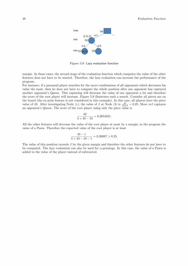
48 Evaluation Function
Figure 5.9: Lazy evaluation function
margin. In those cases, the second stage of the evaluation function which computes the value of the otherfeatures does not have to be started. Therefore, the lazy evaluation can increase the performance of theprogram.For instance, if a paranoid player searches for the move combination of all opponents which decreases hisvalue the most, then he does not have to compute the whole position after one opponent has capturedanother opponent’s Queen. This capturing will decrease the value of one opponent a lot and thereforethe score of the root player will increase. Figure 5.9 illustrates such a search. Consider all pieces are onthe board (the en prise feature is not considered in this example). In this case, all players have the piecevalue of 43. After investigating Node (c), the value of β at Node (b) is 43
43×4 = 0.25. Move m3 capturesan opponent’s Queen. The score of the root player using only the piece value is
43
4× 43− 10= 0.2654321.
All the other features will decrease the value of the root player at most by a margin, in the program thevalue of a Pawn. Therefore the expected value of the root player is at least
43− 1
4× 43− 10− 1= 0.26087 > 0.25.
The value of this position exceeds β by the given margin and therefore the other features do not have tobe computed. The lazy evaluation can also be used for α-prunings. In this case, the value of a Pawn isadded to the value of the player instead of subtracted.
Chapter 6
Experiments and Results
In this chapter, the experiments performed with the program for playing multi-player Chess, developedin Java 1.6.0, and the corresponding results are presented. The settings of the experiments are explainedin Section 6.1. The results of the experiments performed to test the quiescence search are shown inSection 6.2. In Section 6.3, the performance of the three existing algorithms, paranoid, maxn and best-reply search, are presented. The questions (see Section 4.2) regarding the move ordering in the proposedbest-reply variants are answered by experiments in Section 6.4. Afterwards, the strength of the proposedbest-reply variants are compared in Section 6.5. The strongest of the best-reply variants is compared tothe existing algorithms paranoid, maxn and best-reply in Section 6.6. A conclusion of all the performedexperiments is given in Section 6.7.For all tables in this chapter, the numbers in the brackets indicate the win ratio, applied with a 95%confidence interval. The columns labelled with ‘Time’ state the time in milliseconds each player had forcomputing the move he considers best and the columns labelled with ‘Games’ indicate how many gameswere played.
6.1 Settings
Multi-player Chess is always played with four players. Table 6.1 shows all the possible settings forcomparing two, three and four different algorithms against each other. The position of the players caninfluence their strength and therefore all possible combinations have to be used in the experiments togain reliable results. For comparing two algorithms against each other, there exist 14 combinations (seeSubtable 6.1(a)). Six of these 14 combinations consist of two players using one algorithm and two playersusing another algorithm. The eight remaining combinations consist of one player using one algorithmagainst three players using another algorithm. For comparing three algorithms against each other, one ofthe algorithms has to be played by two players. There exist 36 combinations as depicted in 6.1(b). The24 combinations for comparing four algorithms against each other are depicted in 6.1(c).In the maxn algorithm shallow pruning, described in Subsection 3.3.1, is applied. In all the other algo-rithms, αβ-pruning (see Subsection 3.1.1) is applied. In all algorithms, the search enhancements describedin Section 3.2 are used for the searching players. To find out whether the transposition tables, killer movesand history heuristics are also useful for the non-searching opponents, experiments are performed in Sub-section 6.4.3. All the experiments are performed on 64-Bit Linux machines with a speed of 2.4 GHz.
6.2 Quiescence Search
In this section, the usability of the quiescence search (Section 3.4) is tested for the three search algorithmsparanoid (Subsection 6.2.1), maxn (Subsection 6.2.2) and best-reply (Subsection 6.2.3). Subsection 6.2.4gives a summarization and an explanation of the results.
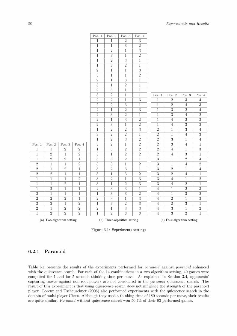
50 Experiments and Results
Pos. 1 Pos. 2 Pos. 3 Pos. 4
1 1 2 21 2 1 21 2 2 12 1 1 22 1 2 12 2 1 11 1 1 21 1 2 11 2 1 12 1 1 12 2 2 12 2 1 22 1 2 21 2 2 2
(a) Two-algorithm setting
Pos. 1 Pos. 2 Pos. 3 Pos. 4
1 1 2 31 1 3 21 2 1 31 3 1 21 2 3 11 3 2 12 1 1 33 1 1 22 1 3 13 1 2 12 3 1 13 2 1 12 2 1 32 2 3 12 1 2 32 3 2 12 1 3 22 3 1 21 2 2 33 2 2 11 2 3 23 2 1 21 3 2 23 1 2 23 3 2 13 3 1 23 2 3 13 1 3 23 2 1 33 1 2 32 3 3 11 3 3 22 3 1 31 3 2 32 1 3 31 2 3 3
(b) Three-algorithm setting
Pos. 1 Pos. 2 Pos. 3 Pos. 4
1 2 3 41 2 4 31 3 2 41 3 4 21 4 2 31 4 3 22 1 3 42 1 4 32 3 1 42 3 4 12 4 1 32 4 3 13 1 2 43 1 4 23 2 1 43 2 4 13 4 1 23 4 2 14 1 2 34 1 3 24 2 1 34 2 3 14 3 1 24 3 2 1
(c) Four-algorithm setting
Figure 6.1: Experiments settings
6.2.1 Paranoid
Table 6.1 presents the results of the experiments performed for paranoid against paranoid enhancedwith the quiescence search. For each of the 14 combinations in a two-algorithm setting, 40 games werecomputed for 1 and for 5 seconds thinking time per move. As explained in Section 3.4, opponents’capturing moves against non-root-players are not considered in the paranoid quiescence search. Theresult of this experiment is that using quiescence search does not influence the strength of the paranoidplayer. Lorenz and Tscheuschner (2006) also performed experiments with the quiescence search in thedomain of multi-player Chess. Although they used a thinking time of 180 seconds per move, their resultsare quite similar. Paranoid without quiescence search won 50.4% of their 93 performed games.
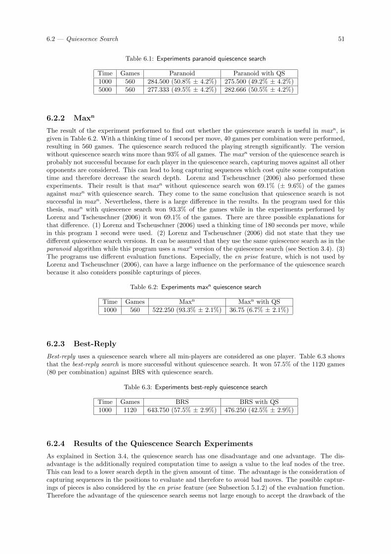
6.2 — Quiescence Search 51
Table 6.1: Experiments paranoid quiescence search
Time Games Paranoid Paranoid with QS1000 560 284.500 (50.8% ± 4.2%) 275.500 (49.2% ± 4.2%)5000 560 277.333 (49.5% ± 4.2%) 282.666 (50.5% ± 4.2%)
6.2.2 Maxn
The result of the experiment performed to find out whether the quiescence search is useful in maxn, isgiven in Table 6.2. With a thinking time of 1 second per move, 40 games per combination were performed,resulting in 560 games. The quiescence search reduced the playing strength significantly. The versionwithout quiescence search wins more than 93% of all games. The maxn version of the quiescence search isprobably not successful because for each player in the quiescence search, capturing moves against all otheropponents are considered. This can lead to long capturing sequences which cost quite some computationtime and therefore decrease the search depth. Lorenz and Tscheuschner (2006) also performed theseexperiments. Their result is that maxn without quiescence search won 69.1% (± 9.6%) of the gamesagainst maxn with quiescence search. They come to the same conclusion that quiescence search is notsuccessful in maxn. Nevertheless, there is a large difference in the results. In the program used for thisthesis, maxn with quiescence search won 93.3% of the games while in the experiments performed byLorenz and Tscheuschner (2006) it won 69.1% of the games. There are three possible explanations forthat difference. (1) Lorenz and Tscheuschner (2006) used a thinking time of 180 seconds per move, whilein this program 1 second were used. (2) Lorenz and Tscheuschner (2006) did not state that they usedifferent quiescence search versions. It can be assumed that they use the same quiescence search as in theparanoid algorithm while this program uses a maxn version of the quiescence search (see Section 3.4). (3)The programs use different evaluation functions. Especially, the en prise feature, which is not used byLorenz and Tscheuschner (2006), can have a large influence on the performance of the quiescence searchbecause it also considers possible capturings of pieces.
Table 6.2: Experiments maxn quiescence search
Time Games Maxn Maxn with QS1000 560 522.250 (93.3% ± 2.1%) 36.75 (6.7% ± 2.1%)
6.2.3 Best-Reply
Best-reply uses a quiescence search where all min-players are considered as one player. Table 6.3 showsthat the best-reply search is more successful without quiescence search. It won 57.5% of the 1120 games(80 per combination) against BRS with quiescence search.
Table 6.3: Experiments best-reply quiescence search
Time Games BRS BRS with QS1000 1120 643.750 (57.5% ± 2.9%) 476.250 (42.5% ± 2.9%)
6.2.4 Results of the Quiescence Search Experiments
As explained in Section 3.4, the quiescence search has one disadvantage and one advantage. The dis-advantage is the additionally required computation time to assign a value to the leaf nodes of the tree.This can lead to a lower search depth in the given amount of time. The advantage is the consideration ofcapturing sequences in the positions to evaluate and therefore to avoid bad moves. The possible captur-ings of pieces is also considered by the en prise feature (see Subsection 5.1.2) of the evaluation function.Therefore the advantage of the quiescence search seems not large enough to accept the drawback of the
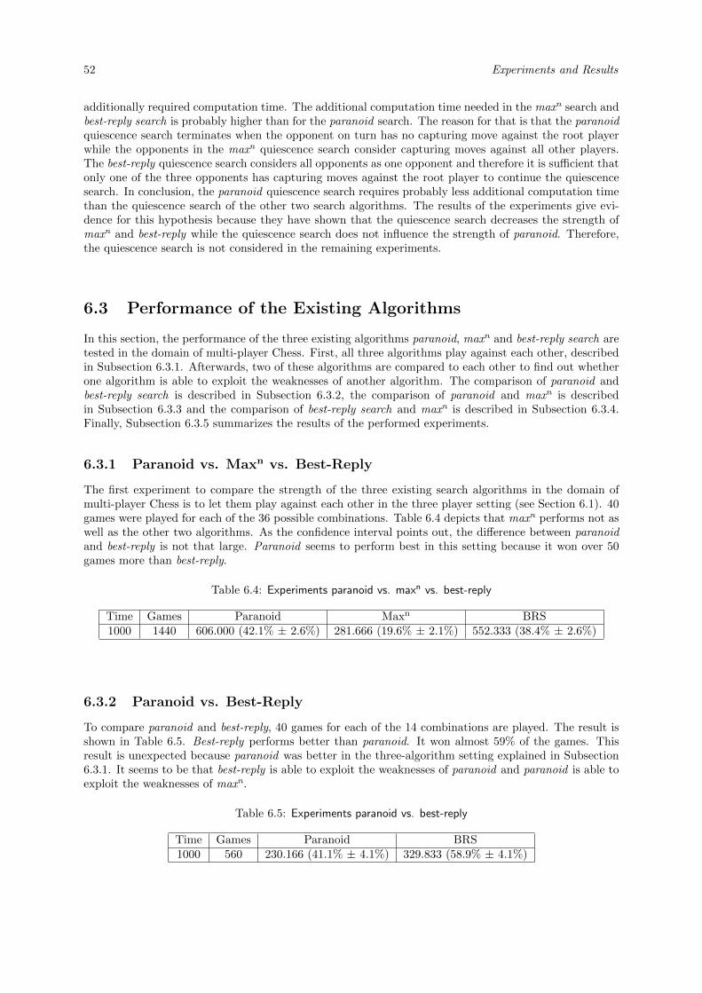
52 Experiments and Results
additionally required computation time. The additional computation time needed in the maxn search andbest-reply search is probably higher than for the paranoid search. The reason for that is that the paranoidquiescence search terminates when the opponent on turn has no capturing move against the root playerwhile the opponents in the maxn quiescence search consider capturing moves against all other players.The best-reply quiescence search considers all opponents as one opponent and therefore it is sufficient thatonly one of the three opponents has capturing moves against the root player to continue the quiescencesearch. In conclusion, the paranoid quiescence search requires probably less additional computation timethan the quiescence search of the other two search algorithms. The results of the experiments give evi-dence for this hypothesis because they have shown that the quiescence search decreases the strength ofmaxn and best-reply while the quiescence search does not influence the strength of paranoid. Therefore,the quiescence search is not considered in the remaining experiments.
6.3 Performance of the Existing Algorithms
In this section, the performance of the three existing algorithms paranoid, maxn and best-reply search aretested in the domain of multi-player Chess. First, all three algorithms play against each other, describedin Subsection 6.3.1. Afterwards, two of these algorithms are compared to each other to find out whetherone algorithm is able to exploit the weaknesses of another algorithm. The comparison of paranoid andbest-reply search is described in Subsection 6.3.2, the comparison of paranoid and maxn is describedin Subsection 6.3.3 and the comparison of best-reply search and maxn is described in Subsection 6.3.4.Finally, Subsection 6.3.5 summarizes the results of the performed experiments.
6.3.1 Paranoid vs. Maxn vs. Best-Reply
The first experiment to compare the strength of the three existing search algorithms in the domain ofmulti-player Chess is to let them play against each other in the three player setting (see Section 6.1). 40games were played for each of the 36 possible combinations. Table 6.4 depicts that maxn performs not aswell as the other two algorithms. As the confidence interval points out, the difference between paranoidand best-reply is not that large. Paranoid seems to perform best in this setting because it won over 50games more than best-reply.
Table 6.4: Experiments paranoid vs. maxn vs. best-reply
Time Games Paranoid Maxn BRS1000 1440 606.000 (42.1% ± 2.6%) 281.666 (19.6% ± 2.1%) 552.333 (38.4% ± 2.6%)
6.3.2 Paranoid vs. Best-Reply
To compare paranoid and best-reply, 40 games for each of the 14 combinations are played. The result isshown in Table 6.5. Best-reply performs better than paranoid. It won almost 59% of the games. Thisresult is unexpected because paranoid was better in the three-algorithm setting explained in Subsection6.3.1. It seems to be that best-reply is able to exploit the weaknesses of paranoid and paranoid is able toexploit the weaknesses of maxn.
Table 6.5: Experiments paranoid vs. best-reply
Time Games Paranoid BRS1000 560 230.166 (41.1% ± 4.1%) 329.833 (58.9% ± 4.1%)
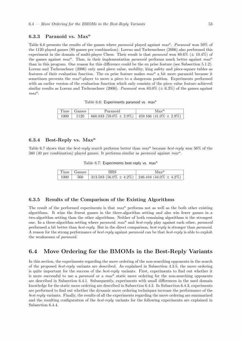
6.4 — Move Ordering for the BMOMs in the Best-Reply Variants 53
6.3.3 Paranoid vs. Maxn
Table 6.6 presents the results of the games where paranoid played against maxn. Paranoid won 59% ofthe 1120 played games (80 games per combination). Lorenz and Tscheuschner (2006) also performed thisexperiment in the domain of multi-player Chess. Their result is that paranoid won 89.6% (± 10.4%) ofthe games against maxn. Thus, in their implementation paranoid performs much better against maxn
than in this program. One reason for this difference could be the en prise feature (see Subsection 5.1.2).Lorenz and Tscheuschner (2006) only used piece value, mobility, king safety and piece-square tables asfeatures of their evaluation function. The en prise feature makes maxn a bit more paranoid because itsometimes prevents the maxn-player to move a piece to a dangerous position. Experiments performedwith an earlier version of the evaluation function which only consists of the piece value feature achievedsimilar results as Lorenz and Tscheuschner (2006). Paranoid won 83.0% (± 6.3%) of the games againstmaxn.
Table 6.6: Experiments paranoid vs. maxn
Time Games Paranoid Maxn
1000 1120 660.833 (59.0% ± 2.9%) 459.166 (41.0% ± 2.9%)
6.3.4 Best-Reply vs. Maxn
Table 6.7 shows that the best-reply search performs better than maxn because best-reply won 56% of the560 (40 per combination) played games. It performs similar as paranoid against maxn.
Table 6.7: Experiments best-reply vs. maxn
Time Games BRS Maxn
1000 560 313.583 (56.0% ± 4.2%) 246.416 (44.0% ± 4.2%)
6.3.5 Results of the Comparison of the Existing Algorithms
The result of the performed experiments is that maxn performs not as well as the both other existingalgorithms. It wins the fewest games in the three-algorithm setting and also win fewer games in atwo-algorithm setting than the other algorithms. Neither of both remaining algorithms is the strongestone. In a three-algorithm setting where paranoid, maxn and best-reply play against each other, paranoidperformed a bit better than best-reply. But in the direct comparison, best-reply is stronger than paranoid.A reason for the strong performance of best-reply against paranoid can be that best-reply is able to exploitthe weaknesses of paranoid.
6.4 Move Ordering for the BMOMs in the Best-Reply Variants
In this section, the experiments regarding the move ordering of the non-searching opponents in the searchof the proposed best-reply variants are described. As explained in Subsection 4.3.5, the move orderingis quite important for the success of the best-reply variants. First, experiments to find out whether itis more successful to use a paranoid or a maxn static move ordering for the non-searching opponentsare described in Subsection 6.4.1. Subsequently, experiments with small differences in the used domainknowledge for the static move ordering are described in Subsection 6.4.2. In Subsection 6.4.3, experimentsare performed to find out whether the dynamic move ordering techniques increase the performance of thebest-reply variants. Finally, the results of all the experiments regarding the move ordering are summarizedand the resulting configuration of the best-reply variants for the following experiments are explained inSubsection 6.4.4.
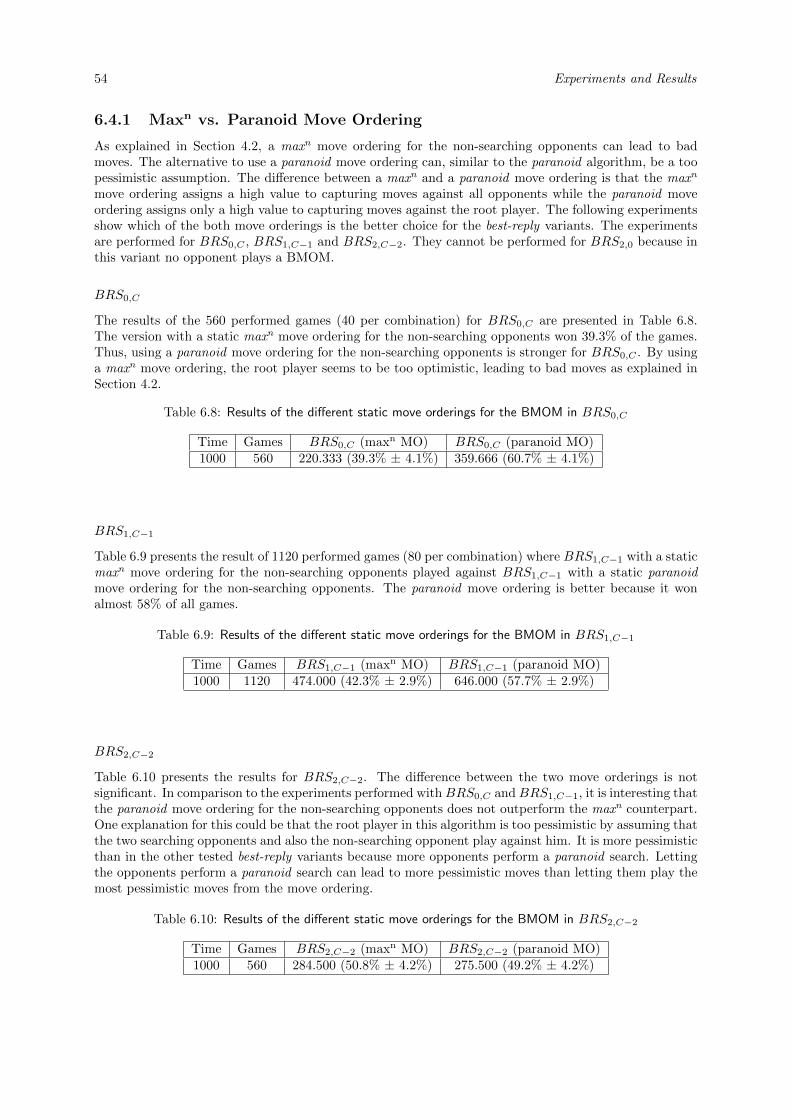
54 Experiments and Results
6.4.1 Maxn vs. Paranoid Move Ordering
As explained in Section 4.2, a maxn move ordering for the non-searching opponents can lead to badmoves. The alternative to use a paranoid move ordering can, similar to the paranoid algorithm, be a toopessimistic assumption. The difference between a maxn and a paranoid move ordering is that the maxn
move ordering assigns a high value to capturing moves against all opponents while the paranoid moveordering assigns only a high value to capturing moves against the root player. The following experimentsshow which of the both move orderings is the better choice for the best-reply variants. The experimentsare performed for BRS0,C , BRS1,C−1 and BRS2,C−2. They cannot be performed for BRS2,0 because inthis variant no opponent plays a BMOM.
BRS0,C
The results of the 560 performed games (40 per combination) for BRS0,C are presented in Table 6.8.The version with a static maxn move ordering for the non-searching opponents won 39.3% of the games.Thus, using a paranoid move ordering for the non-searching opponents is stronger for BRS0,C . By usinga maxn move ordering, the root player seems to be too optimistic, leading to bad moves as explained inSection 4.2.
Table 6.8: Results of the different static move orderings for the BMOM in BRS0,C
Time Games BRS0,C (maxn MO) BRS0,C (paranoid MO)1000 560 220.333 (39.3% ± 4.1%) 359.666 (60.7% ± 4.1%)
BRS1,C−1
Table 6.9 presents the result of 1120 performed games (80 per combination) where BRS1,C−1 with a staticmaxn move ordering for the non-searching opponents played against BRS1,C−1 with a static paranoidmove ordering for the non-searching opponents. The paranoid move ordering is better because it wonalmost 58% of all games.
Table 6.9: Results of the different static move orderings for the BMOM in BRS1,C−1
Time Games BRS1,C−1 (maxn MO) BRS1,C−1 (paranoid MO)1000 1120 474.000 (42.3% ± 2.9%) 646.000 (57.7% ± 2.9%)
BRS2,C−2
Table 6.10 presents the results for BRS2,C−2. The difference between the two move orderings is notsignificant. In comparison to the experiments performed withBRS0,C andBRS1,C−1, it is interesting thatthe paranoid move ordering for the non-searching opponents does not outperform the maxn counterpart.One explanation for this could be that the root player in this algorithm is too pessimistic by assuming thatthe two searching opponents and also the non-searching opponent play against him. It is more pessimisticthan in the other tested best-reply variants because more opponents perform a paranoid search. Lettingthe opponents perform a paranoid search can lead to more pessimistic moves than letting them play themost pessimistic moves from the move ordering.
Table 6.10: Results of the different static move orderings for the BMOM in BRS2,C−2
Time Games BRS2,C−2 (maxn MO) BRS2,C−2 (paranoid MO)1000 560 284.500 (50.8% ± 4.2%) 275.500 (49.2% ± 4.2%)
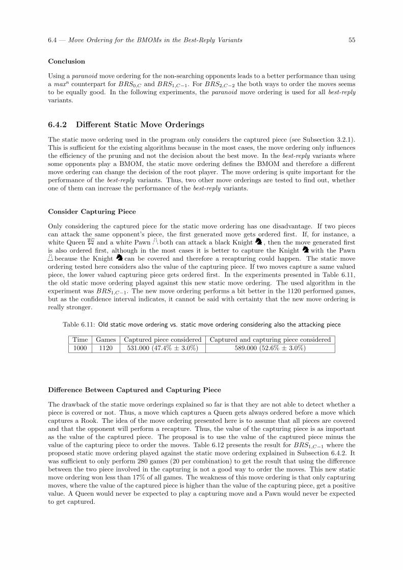
6.4 — Move Ordering for the BMOMs in the Best-Reply Variants 55
Conclusion
Using a paranoid move ordering for the non-searching opponents leads to a better performance than usinga maxn counterpart for BRS0,C and BRS1,C−1. For BRS2,C−2 the both ways to order the moves seemsto be equally good. In the following experiments, the paranoid move ordering is used for all best-replyvariants.
6.4.2 Different Static Move Orderings
The static move ordering used in the program only considers the captured piece (see Subsection 3.2.1).This is sufficient for the existing algorithms because in the most cases, the move ordering only influencesthe efficiency of the pruning and not the decision about the best move. In the best-reply variants wheresome opponents play a BMOM, the static move ordering defines the BMOM and therefore a differentmove ordering can change the decision of the root player. The move ordering is quite important for theperformance of the best-reply variants. Thus, two other move orderings are tested to find out, whetherone of them can increase the performance of the best-reply variants.
Consider Capturing Piece
Only considering the captured piece for the static move ordering has one disadvantage. If two piecescan attack the same opponent’s piece, the first generated move gets ordered first. If, for instance, awhite Queen and a white Pawn both can attack a black Knight , then the move generated firstis also ordered first, although in the most cases it is better to capture the Knight with the Pawn
because the Knight can be covered and therefore a recapturing could happen. The static moveordering tested here considers also the value of the capturing piece. If two moves capture a same valuedpiece, the lower valued capturing piece gets ordered first. In the experiments presented in Table 6.11,the old static move ordering played against this new static move ordering. The used algorithm in theexperiment was BRS1,C−1. The new move ordering performs a bit better in the 1120 performed games,but as the confidence interval indicates, it cannot be said with certainty that the new move ordering isreally stronger.
Table 6.11: Old static move ordering vs. static move ordering considering also the attacking piece
Time Games Captured piece considered Captured and capturing piece considered1000 1120 531.000 (47.4% ± 3.0%) 589.000 (52.6% ± 3.0%)
Difference Between Captured and Capturing Piece
The drawback of the static move orderings explained so far is that they are not able to detect whether apiece is covered or not. Thus, a move which captures a Queen gets always ordered before a move whichcaptures a Rook. The idea of the move ordering presented here is to assume that all pieces are coveredand that the opponent will perform a recapture. Thus, the value of the capturing piece is as importantas the value of the captured piece. The proposal is to use the value of the captured piece minus thevalue of the capturing piece to order the moves. Table 6.12 presents the result for BRS1,C−1 where theproposed static move ordering played against the static move ordering explained in Subsection 6.4.2. Itwas sufficient to only perform 280 games (20 per combination) to get the result that using the differencebetween the two piece involved in the capturing is not a good way to order the moves. This new staticmove ordering won less than 17% of all games. The weakness of this move ordering is that only capturingmoves, where the value of the captured piece is higher than the value of the capturing piece, get a positivevalue. A Queen would never be expected to play a capturing move and a Pawn would never be expectedto get captured.
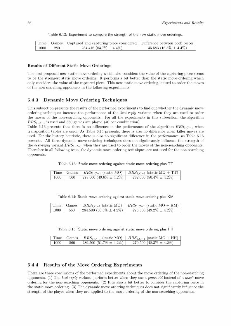
56 Experiments and Results
Table 6.12: Experiment to compare the strength of the new static move orderings.
Time Games Captured and capturing piece considered Difference between both pieces1000 280 234.416 (83.7% ± 4.4%) 45.583 (16.3% ± 4.4%)
Results of Different Static Move Orderings
The first proposed new static move ordering which also considers the value of the capturing piece seemsto be the strongest static move ordering. It performs a bit better than the static move ordering whichonly considers the value of the captured piece. This new static move ordering is used to order the movesof the non-searching opponents in the following experiments.
6.4.3 Dynamic Move Ordering Techniques
This subsection presents the results of the performed experiments to find out whether the dynamic moveordering techniques increase the performance of the best-reply variants when they are used to orderthe moves of the non-searching opponents. For all the experiments in this subsection, the algorithmBRS1,C−1 is used and 560 games are played (40 per combination).Table 6.13 presents that there is no difference in the performance of the algorithm BRS1,C−1 whentransposition tables are used. As Table 6.14 presents, there is also no difference when killer moves areused. For the history heuristic, there is also no significant difference in the performance, as Table 6.15presents. All three dynamic move ordering techniques does not significantly influence the strength ofthe best-reply variant BRS1,C−1 when they are used to order the moves of the non-searching opponents.Therefore in all following tests, the dynamic move ordering techniques are not used for the non-searchingopponents.
Table 6.13: Static move ordering against static move ordering plus TT
Time Games BRS1,C−1 (static MO) BRS1,C−1 (static MO + TT)1000 560 278.000 (49.6% ± 4.2%) 282.000 (50.4% ± 4.2%)
Table 6.14: Static move ordering against static move ordering plus KM
Time Games BRS1,C−1 (static MO) BRS1,C−1 (static MO + KM)1000 560 284.500 (50.8% ± 4.2%) 275.500 (49.2% ± 4.2%)
Table 6.15: Static move ordering against static move ordering plus HH
Time Games BRS1,C−1 (static MO) BRS1,C−1 (static MO + HH)1000 560 289.500 (51.7% ± 4.2%) 270.500 (48.3% ± 4.2%)
6.4.4 Results of the Move Ordering Experiments
There are three conclusions of the performed experiments about the move ordering of the non-searchingopponents. (1) The best-reply variants perform better when they use a paranoid instead of a maxn moveordering for the non-searching opponents. (2) It is also a bit better to consider the capturing piece inthe static move ordering. (3) The dynamic move ordering techniques does not significantly influence thestrength of the player when they are applied to the move ordering of the non-searching opponents.
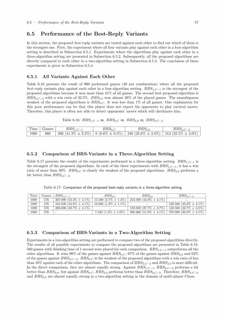
6.5 — Performance of the Best-Reply Variants 57
6.5 Performance of the Best-Reply Variants
In this section, the proposed best-reply variants are tested against each other to find out which of them isthe strongest one. First, the experiment where all four variants play against each other in a four-algorithmsetting is described in Subsection 6.5.1. Experiments where the algorithms play against each other in athree-algorithm setting are presented in Subsection 6.5.2. Subsequently, all the proposed algorithms aredirectly compared to each other in a two-algorithm setting in Subsection 6.5.3. The conclusion of theseexperiments is given in Subsection 6.5.4.
6.5.1 All Variants Against Each Other
Table 6.16 presents the result of 960 performed games (40 per combination) where all the proposedbest-reply variants play against each other in a four-algorithm setting. BRS1,C−1 is the strongest of theproposed algorithms because it won more than 41% of all games. The second best proposed algorithm isBRS2,C−2 with a win ratio of 32.5%. BRS2,0 won almost 26% of the played games. The unambiguousweakest of the proposed algorithms is BRS0,C . It won less than 1% of all games. One explanation forthis poor performance can be that this player does not expect his opponents to play tactical moves.Therefore, this player is often not able to detect opponents’ moves which will checkmate him.
Table 6.16: BRS1,C−1 vs. BRS0,C vs. BRS2,0 vs. BRS2,C−2
Time Games BRS1,C−1 BRS0,C BRS2,0 BRS2,C−21000 960 396 (41.3% ± 3.2%) 6 (0.6% ± 0.5%) 246 (25.6% ± 2.8%) 312 (32.5% ± 3.0%)
6.5.2 Comparison of BRS-Variants in a Three-Algorithm Setting
Table 6.17 presents the results of the experiments performed in a three-algorithm setting. BRS1,C−1 isthe strongest of the proposed algorithms. In each of the three experiments with BRS1,C−1, it has a winratio of more than 49%. BRS0,C is clearly the weakest of the proposed algorithms. BRS2,0 performs abit better than BRS2,C−2.
Table 6.17: Comparison of the proposed best-reply variants in a three-algorithm setting
Time Games BRS1,C−1 BRS0,C BRS2,0 BRS2,C−21000 576 307.000 (53.3% ± 4.1%) 15.500 (2.7% ± 1.4%) 253.500 (44.0% ± 4.1%) -1000 576 316.500 (54.9% ± 4.1%) 10.000 (1.8% ± 1.1%) - 249.500 (43.3% ± 4.1%)1000 576 286.000 (49.7% ± 4.1%) - 159.500 (27.7% ± 3.7%) 130.500 (22.7% ± 3.5%)1000 576 - 7.333 (1.3% ± 1.0%) 298.666 (51.9% ± 4.1%) 270.000 (46.9% ± 4.1%)
6.5.3 Comparison of BRS-Variants in a Two-Algorithm Setting
Experiments in a two-algorithm setting are performed to compare two of the proposed algorithms directly.The results of all possible experiments to compare the proposed algorithms are presented in Table 6.18.560 games with thinking time of 1 second were played for each comparison. BRS1,C−1 outperforms all theother algorithms. It wins 98% of the games against BRS0,C , 67% of the games against BRS2,0 and 62%of the games against BRS2,C−2. BRS0,C is the weakest of the proposed algorithms with a win ratio of lessthan 10% against each of the other algorithms. The comparison of BRS2,C−2 and BRS2,0 is more difficult.In the direct comparison, they are almost equally strong. Against BRS1,C−1, BRS2,C−2 performs a bitbetter than BRS2,0, but against BRS0,C , BRS2,0 performs better than BRS2,C−2. Therefore, BRS2,C−2and BRS2,0 are almost equally strong in a two-algorithm setting in the domain of multi-player Chess.
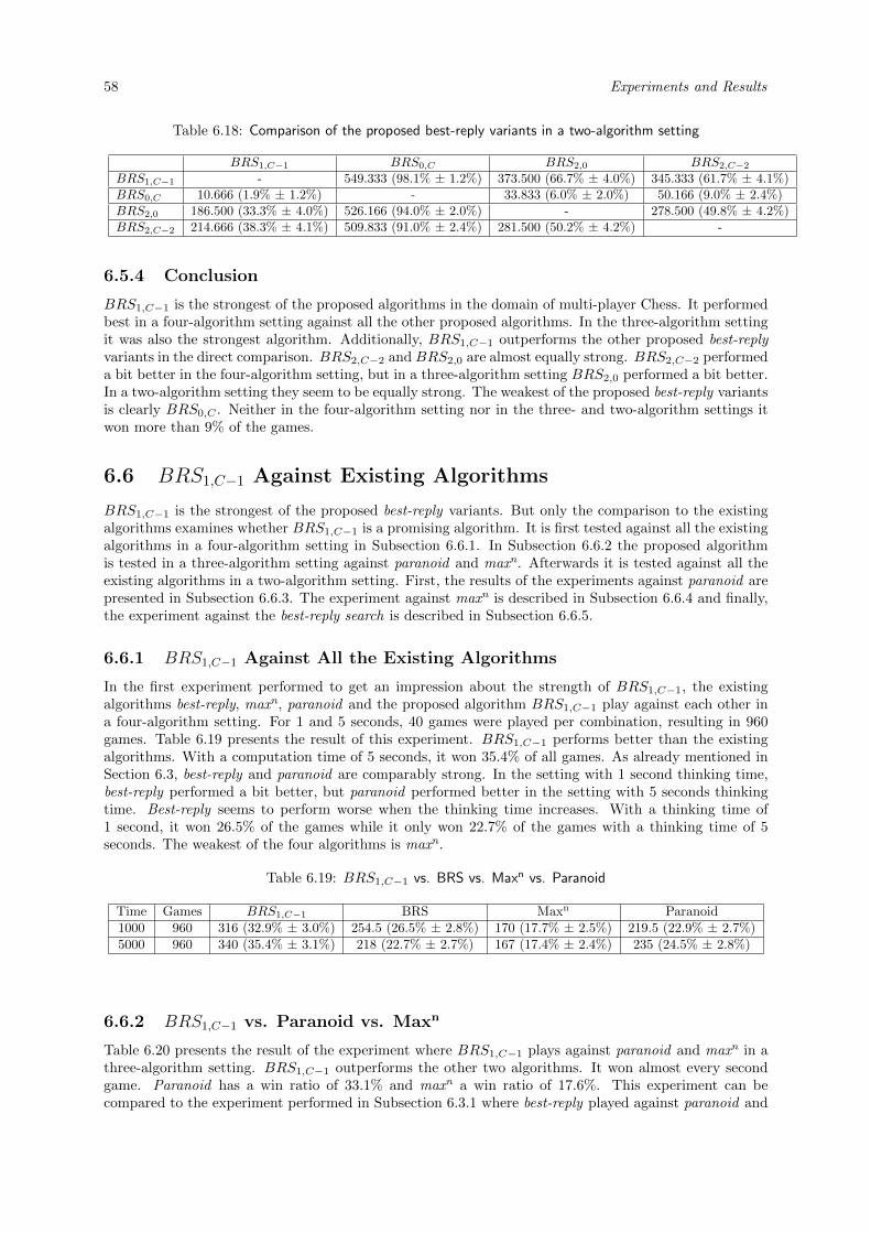
58 Experiments and Results
Table 6.18: Comparison of the proposed best-reply variants in a two-algorithm setting
BRS1,C−1 BRS0,C BRS2,0 BRS2,C−2BRS1,C−1 - 549.333 (98.1% ± 1.2%) 373.500 (66.7% ± 4.0%) 345.333 (61.7% ± 4.1%)BRS0,C 10.666 (1.9% ± 1.2%) - 33.833 (6.0% ± 2.0%) 50.166 (9.0% ± 2.4%)BRS2,0 186.500 (33.3% ± 4.0%) 526.166 (94.0% ± 2.0%) - 278.500 (49.8% ± 4.2%)BRS2,C−2 214.666 (38.3% ± 4.1%) 509.833 (91.0% ± 2.4%) 281.500 (50.2% ± 4.2%) -
6.5.4 Conclusion
BRS1,C−1 is the strongest of the proposed algorithms in the domain of multi-player Chess. It performedbest in a four-algorithm setting against all the other proposed algorithms. In the three-algorithm settingit was also the strongest algorithm. Additionally, BRS1,C−1 outperforms the other proposed best-replyvariants in the direct comparison. BRS2,C−2 and BRS2,0 are almost equally strong. BRS2,C−2 performeda bit better in the four-algorithm setting, but in a three-algorithm setting BRS2,0 performed a bit better.In a two-algorithm setting they seem to be equally strong. The weakest of the proposed best-reply variantsis clearly BRS0,C . Neither in the four-algorithm setting nor in the three- and two-algorithm settings itwon more than 9% of the games.
6.6 BRS1,C−1 Against Existing Algorithms
BRS1,C−1 is the strongest of the proposed best-reply variants. But only the comparison to the existingalgorithms examines whether BRS1,C−1 is a promising algorithm. It is first tested against all the existingalgorithms in a four-algorithm setting in Subsection 6.6.1. In Subsection 6.6.2 the proposed algorithmis tested in a three-algorithm setting against paranoid and maxn. Afterwards it is tested against all theexisting algorithms in a two-algorithm setting. First, the results of the experiments against paranoid arepresented in Subsection 6.6.3. The experiment against maxn is described in Subsection 6.6.4 and finally,the experiment against the best-reply search is described in Subsection 6.6.5.
6.6.1 BRS1,C−1 Against All the Existing Algorithms
In the first experiment performed to get an impression about the strength of BRS1,C−1, the existingalgorithms best-reply, maxn, paranoid and the proposed algorithm BRS1,C−1 play against each other ina four-algorithm setting. For 1 and 5 seconds, 40 games were played per combination, resulting in 960games. Table 6.19 presents the result of this experiment. BRS1,C−1 performs better than the existingalgorithms. With a computation time of 5 seconds, it won 35.4% of all games. As already mentioned inSection 6.3, best-reply and paranoid are comparably strong. In the setting with 1 second thinking time,best-reply performed a bit better, but paranoid performed better in the setting with 5 seconds thinkingtime. Best-reply seems to perform worse when the thinking time increases. With a thinking time of1 second, it won 26.5% of the games while it only won 22.7% of the games with a thinking time of 5seconds. The weakest of the four algorithms is maxn.
Table 6.19: BRS1,C−1 vs. BRS vs. Maxn vs. Paranoid
Time Games BRS1,C−1 BRS Maxn Paranoid1000 960 316 (32.9% ± 3.0%) 254.5 (26.5% ± 2.8%) 170 (17.7% ± 2.5%) 219.5 (22.9% ± 2.7%)5000 960 340 (35.4% ± 3.1%) 218 (22.7% ± 2.7%) 167 (17.4% ± 2.4%) 235 (24.5% ± 2.8%)
6.6.2 BRS1,C−1 vs. Paranoid vs. Maxn
Table 6.20 presents the result of the experiment where BRS1,C−1 plays against paranoid and maxn in athree-algorithm setting. BRS1,C−1 outperforms the other two algorithms. It won almost every secondgame. Paranoid has a win ratio of 33.1% and maxn a win ratio of 17.6%. This experiment can becompared to the experiment performed in Subsection 6.3.1 where best-reply played against paranoid and
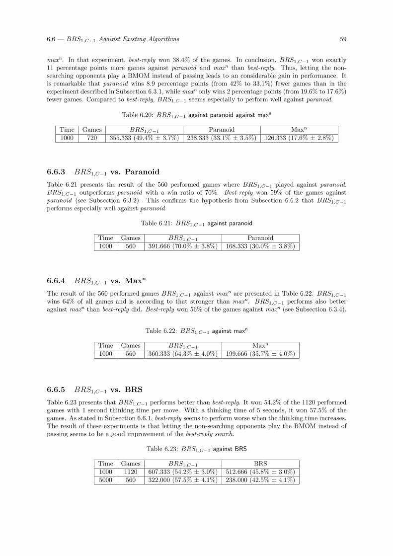
6.6 — BRS1,C−1 Against Existing Algorithms 59
maxn. In that experiment, best-reply won 38.4% of the games. In conclusion, BRS1,C−1 won exactly11 percentage points more games against paranoid and maxn than best-reply. Thus, letting the non-searching opponents play a BMOM instead of passing leads to an considerable gain in performance. Itis remarkable that paranoid wins 8.9 percentage points (from 42% to 33.1%) fewer games than in theexperiment described in Subsection 6.3.1, while maxn only wins 2 percentage points (from 19.6% to 17.6%)fewer games. Compared to best-reply, BRS1,C−1 seems especially to perform well against paranoid.
Table 6.20: BRS1,C−1 against paranoid against maxn
Time Games BRS1,C−1 Paranoid Maxn
1000 720 355.333 (49.4% ± 3.7%) 238.333 (33.1% ± 3.5%) 126.333 (17.6% ± 2.8%)
6.6.3 BRS1,C−1 vs. Paranoid
Table 6.21 presents the result of the 560 performed games where BRS1,C−1 played against paranoid.BRS1,C−1 outperforms paranoid with a win ratio of 70%. Best-reply won 59% of the games againstparanoid (see Subsection 6.3.2). This confirms the hypothesis from Subsection 6.6.2 that BRS1,C−1performs especially well against paranoid.
Table 6.21: BRS1,C−1 against paranoid
Time Games BRS1,C−1 Paranoid1000 560 391.666 (70.0% ± 3.8%) 168.333 (30.0% ± 3.8%)
6.6.4 BRS1,C−1 vs. Maxn
The result of the 560 performed games BRS1,C−1 against maxn are presented in Table 6.22. BRS1,C−1wins 64% of all games and is according to that stronger than maxn. BRS1,C−1 performs also betteragainst maxn than best-reply did. Best-reply won 56% of the games against maxn (see Subsection 6.3.4).
Table 6.22: BRS1,C−1 against maxn
Time Games BRS1,C−1 Maxn
1000 560 360.333 (64.3% ± 4.0%) 199.666 (35.7% ± 4.0%)
6.6.5 BRS1,C−1 vs. BRS
Table 6.23 presents that BRS1,C−1 performs better than best-reply. It won 54.2% of the 1120 performedgames with 1 second thinking time per move. With a thinking time of 5 seconds, it won 57.5% of thegames. As stated in Subsection 6.6.1, best-reply seems to perform worse when the thinking time increases.The result of these experiments is that letting the non-searching opponents play the BMOM instead ofpassing seems to be a good improvement of the best-reply search.
Table 6.23: BRS1,C−1 against BRS
Time Games BRS1,C−1 BRS1000 1120 607.333 (54.2% ± 3.0%) 512.666 (45.8% ± 3.0%)5000 560 322.000 (57.5% ± 4.1%) 238.000 (42.5% ± 4.1%)
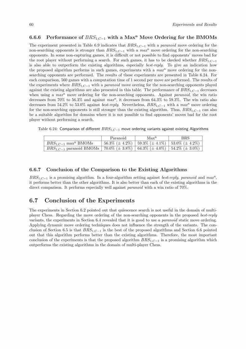
60 Experiments and Results
6.6.6 Performance of BRS1,C−1 with a Maxn Move Ordering for the BMOMs
The experiment presented in Table 6.9 indicates that BRS1,C−1 with a paranoid move ordering for thenon-searching opponents is stronger than BRS1,C−1 with a maxn move ordering for the non-searchingopponents. In some non-capturing games, it is difficult or not possible to find opponents’ moves bad forthe root player without performing a search. For such games, it has to be ckecked whether BRS1,C−1is also able to outperform the existing algorithms, especially best-reply. To give an indication howthe proposed algorithm performs in such games, experiments with a maxn move ordering for the non-searching opponents are performed. The results of these experiments are presented in Table 6.24. Foreach comparison, 560 games with a computation time of 1 second per move are performed. The results ofthe experiments where BRS1,C−1 with a paranoid move orering for the non-searching opponents playedagainst the existing algorithms are also presented in this table. The performance of BRS1,C−1 decreaseswhen using a maxn move ordering for the non-searching opponents. Against paranoid, the win ratiodecreases from 70% to 56.3% and against maxn, it decreases from 64.3% to 59.3%. The win ratio alsodecreases from 54.2% to 53.0% against best-reply. Nevertheless, BRS1,C−1 with a maxn move orderingfor the non-searching opponents is still stronger than the existing algorithm. Thus, BRS1,C−1 can alsobe a suitable algorithm for domains where it is not possible to find opponents’ moves bad for the rootplayer without performing a search.
Table 6.24: Comparison of different BRS1,C−1 move ordering variants against existing Algorithms
Paranoid Maxn BRSBRS1,C−1 maxn BMOMs 56.3% (± 4.2%) 59.3% (± 4.1%) 53.0% (± 4.2%)BRS1,C−1 paranoid BMOMs 70.0% (± 3.8%) 64.3% (± 4.0%) 54.2% (± 3.0%)
6.6.7 Conclusion of the Comparison to the Existing Algorithms
BRS1,C−1 is a promising algorithm. In a four-algorithm setting against best-reply, paranoid and maxn,it performs better than the other algorithms. It is also better than each of the existing algorithms in thedirect comparison. It performs especially well against paranoid with a win ratio of 70%.
6.7 Conclusion of the Experiments
The experiments in Section 6.2 pointed out that quiescence search is not useful in the domain of multi-player Chess. Regarding the move ordering of the non-searching opponents in the proposed best-replyvariants, the experiments in Section 6.4 revealed that it is good to use a paranoid static move ordering.Applying dynamic move ordering techniques does not influence the strength of the variants. The con-clusion of Section 6.5 is that BRS1,C−1 is the best of the proposed algorithms and Section 6.6 pointedout that this algorithm performs better than the existing algorithms. Therefore, the most importantconclusion of the experiments is that the proposed algorithm BRS1,C−1 is a promising algorithm whichoutperforms the existing algorithms in the domain of multi-player Chess.
Chapter 7
Conclusions and Future Research
In this chapter, the conclusion of this thesis is given. First, the research questions are answered in Section7.1. Afterwards the problem statement is answered in Section 7.2. Finally, the future research is givenin Section 7.3.
7.1 Answering the Research Questions
In this section, the two research question stated in Section 1.3 are recalled and answered.
1. Is the best-reply search better than the well-known paranoid and maxn algorithmsin the domain of non-cooperative multi-player Chess?
This questions is answered by the experiments described in Section 6.3. Best-reply performs better thanmaxn. It won 56% of the games against maxn in the direct comparison. It also performs better thanmaxn in the three-player setting with paranoid as third algorithm. The comparison of the best-reply searchand the paranoid algorithm is more complicated. In the three-player setting mentioned before, paranoidperforms a bit better than best-reply (42% to 38%). In contrast to this result, best-reply performs wellagainst paranoid in the direct comparison. It wins almost 59% of these games. It is remarkable thatbest-reply performs better against paranoid (win ratio 59%) than against maxn (win ratio 56%) in thedirect comparison. In conclusion, best-reply outperforms maxn and has a similar strength as paranoid inthe domain of multi-player Chess.
2. Can we find variants of the best-reply search that are even better?
The conclusion of the experiments performed in Section 6.5 is that BRS1,C−1 is definitely the strongestof the proposed best-reply variants. Further, BRS1,C−1 also outperforms the existing algorithms in thedomain of multi-player Chess. Against best-reply, it has a win ratio of 54.2% with a thinking time of 1second and a win ratio of 57.5% with a thinking time of 5 seconds. It has a win ratio of 70% againstparanoid and 64% against maxn. Thus, BRS1,C−1 is a promising algorithm which performs better thanthe existing algorithms in the domain of multi-player Chess.
7.2 Answering the Problem Statement
The problem statement of the thesis is answered in this section.
How can the best-reply search be modified to outperformthe paranoid algorithm in complex (capturing) multi-player games?
The most promising modification of best-reply search is to let the non-searching opponents play thestrongest move based on the static move ordering instead of passing. The static move ordering is quiteimportant for this modification because the best move regarding this move ordering is the root player’sexpectation of the moves played by the non-searching opponents. A bad static move ordering causesthe algorithm to play bad moves. This modification solves the main problem of best-reply that passing
62 Conclusions and Future Research
can lead to officially unreachable and in some domains illegal board positions. The result of the best-case analysis performed in Section 4.4 is that this modification decreases the number of leaf nodes a bitwhile the number of internal nodes increase. In the domain of multi-player Chess, the number of leafnodes is more important than the number of internal nodes because the evaluation function is more timeconsuming than the move generation.The experiment performed with the modified algorithm, called BRS1,C−1, indicates that this algorithmis promising. It outperforms the existing algorithms paranoid, maxn and best-reply. It performs especiallywell against paranoid.
7.3 Future Research
In this section suggestions for the future research are given. These suggestions can be categorized intoseven categories.
1. Evaluation functionAdditional work can be performed on the evaluation function to increase the playing strength.Although the evaluation function used in the program has more than 10 features, even more featurescan be implemented. For regular Chess there are many features that can be adapted to multi-playerChess to increase the playing strength. Especially, features representing endgame knowledge canbe beneficial because no such feature is included in the current evaluation function. Additionally,experts for multi-player Chess can be searched to retrieve domain knowledge that can be used toadd some more features to the evaluation function. Currently, the evaluation function uses twofeatures for the opening. The performance in this part of the game can be increased by buildingand using opening books. The weights of the different features are tuned by hand or by just a fewexperiments. Therefore the playing strength can be increased by using machine learning techniquesto tune the existing parameters of the evaluation function.
2. Forward pruningForward pruning techniques are not used in the program. In quite some regular Chess programs,forward pruning techniques are applied. Therefore, it can be investigated whether applying for-ward pruning techniques like Null Move (Donninger, 1993), ProbCut (Buro, 1995) and MultiCut(Bjornsson and Marsland, 1999) can increase the playing strength.
3. αβ-enhancementsThe αβ-framework can be enhanced by several techniques like MTD(f) (Plaat et al., 1995) or Prin-cipal Variation Search (Fishburn, Finkel, and Lawless, 1980; Marsland and Campbell, 1982)/Ne-gaScout (Reinefeld, 1983). This can also increase the playing strength.
4. Faster frameworkAs part of this thesis, a framework was implemented from scratch. This was the first time that theauthor of this thesis implemented a framework for playing a multi-player game. A few weeks werespent to optimize the framework, but nevertheless the framework can be even more efficient bychanging some implementation details like using bitboards (Heinz, 1997; Hyatt, 1999; Reul, 2009)to represent the board.
5. Static move orderingAs explained in Subsection 4.3.5, the static move ordering is quite important for the performanceof the proposed algorithms. The static more ordering in the program is quite simple. Spendingmore time to enhance the static move ordering could even increase the performance of BRS1,C−1.One improvement can be to consider check moves. This is not considered in the program becauseit cost some computation time to identify check moves. But for the static move ordering for thenon-searching opponents, this can be a promising approach to improve the quality of the moveordering. Another approach to improve the static move ordering can be the use of piece-squaretables. Piece-square tables can be used to evaluate the position of the piece to move with respectto the kind of the moved piece.
6. Allow non-searching opponents to investigate more than one moveIn the proposed algorithm BRS1,C−1 all but one opponents play the best move regarding the static
7.3 — Future Research 63
move ordering. When check moves are also considered in the static move ordering as proposedabove, the question arises whether it is better to expect the opponent to play a good capture moveor a check move. It could be a promising idea to propose an algorithm where the “non-searchingopponents” are allowed to perform a search with a small branching factor like 2 or 3. In such analgorithm it would be possible to consider check moves and also capture moves for the non-searchingopponents. This modification would increase the complexity of the tree, but it would still be muchsmaller than a paranoid -tree. It has to be tested whether the better estimation of the opponents’moves is worth the higher complexity of the tree.
7. Other domainsThe proposed algorithms are only tested in the domain of multi-player Chess. It has to be testedwhether the best of the proposed algorithms, BRS1,C−1, is also able to outperform the existingalgorithms in other domains. The algorithm can be tested in other capture games and also innon-capture games. Additionally, it can be tested in games with imperfect information. It is fromspecial interest to see how the properties of the different games have an influence on the performanceof BRS1,C−1. In multi-player Chess, the evaluation function is more time consuming than the movegeneration. In other games where the move generation is more complex or the board position isquite easy to evaluate, the larger number of internal nodes compared to best-reply can be such adisadvantage that it is not worth to let the non-searching opponents play a move. Moreover, inmulti-player Chess the opponents’ moves have a quite large influence on the position of the rootplayer. Thus, it is quite important to let each opponent play a move. For other games where theopponents’ moves does not have such a large influence on the root player’s position, for instanceracing-games, it has to be tested whether BRS1,C−1 is also able to outperform best-reply.
64 Conclusions and Future Research
Bibliography
Akl, S.G. and Newborn, M.M. (1977). The Principal Continuation and the Killer Heuristic. 1977 ACMAnnual Conference Proceedings, pp. 466–473, ACM Press, New York, NY, USA.[23]
Allis, L.V. (1994). Searching for Solutions in Games and Artificial Intelligence. Ph.D. thesis, Rijksuni-versiteit Limburg, Maastricht, The Netherlands. [9, 17]
Ash, R. and Bishop, R. (1972). Monopoly as a Markov Process. Mathematics Magazine, Vol. 45, pp.26–29. [7]
Beal, D. and Smith, M. (1994). Random Evaluation in Chess. ICCA Journal, Vol. 17, No. 1, pp. 3–9.[42]
Billings, D., Papp, D., Schaeffer, J., and Szafron, D. (1998). Opponent Modeling in Poker. AAAI 98, pp.493–499, American Association for Artificial Intelligence, Menlo Park, CA, USA. ISBN 0–262–51098–7.[7]
Bjornsson, Y. and Marsland, T.A. (1999). Multi-Cut Alpha-Beta Pruning. Computers and Games (CG98) (eds. H.J. van den Herik and H. Iida), Vol. 1558 of Lecture Notes in Computing Science (LNCS),pp. 15–24. Springer-Verlag, Berlin, Germany. [62]
Breuker, D.M. (1998). Memory versus Search in Games. Ph.D. thesis, Maastricht University, Maastricht,The Netherlands. [21]
Browne, C.B., Powley, E., Whitehouse, D., Lucas, S.M., Cowling, P.I., Rohlfshagen, P., Tavener, S.,Perez, D., Samothrakis, S., and Colton, S. (2012). A Survey of Monte Carlo Tree Search Methods. IEEETransactions on Computational Intelligence and AI in Games, Vol. 4, No. 1, pp. 1–43. [8]
Buro, M. (1995). ProbCut: An Effective Selective Extension of the Alpha-Beta Algorithm. ICCAJournal, Vol. 18, No. 2, pp. 71–76. [62]
Campbell, M. (1985). The graph-history interaction: on ignoring position history. Proceedings of the1985 ACM annual conference on The range of computing : mid-80’s perspective: mid-80’s perspective,ACM ’85, pp. 278–280, ACM, New York, NY, USA. ISBN 0–89791–170–9. [23]
Cazenave, T. (2008). Multi-player Go. Computers and Games (CG 08) (eds. H.J. van den Herik, X.Xu, Z. Ma, and M.H.M. Winands), Vol. 5131 of Lecture Notes in Computer Science (LNCS), pp. 50–59,Springer-Verlag, Berlin, Heidelberg. ISBN 978–3–540–87607–6. [8]
Cazenave, T. and Saffidine, A. (2009). Utilisation de la recherche arborescente Monte-Carlo au Hex.Revue d’Intelligence Artificielle, Vol. 23, Nos. 2–3, pp. 183–202. In French. [8]
Chaslot, G.M.J-B., Winands, M.H.M., Herik, H.J. van den, Uiterwijk, J.W.H.M., and Bouzy, B. (2008a).Progressive Strategies For Monte-Carlo Tree Search. New Mathematics and Natural Computation(NMNC), Vol. 4, No. 03, pp. 343–357. [8, 9]
Chaslot, G., Winands, M.H.M., and Herik, H.J. van den (2008b). Parallel Monte-Carlo Tree Search.Computers and Games (CG 2008) (eds. H.J. van den Herik, X. Xu, Z. Ma, and M.H.M. Winands), Vol.5131 of Lecture Notes in Computer Science (LNCS), pp. 60–71, Springer. ISBN 978–3–540–87607–6.[8]
Costikyan, G. (1994). I Have No Words & I Must Design. Interactive Fantasy, No. 2. [7]
66 BIBLIOGRAPHY
Coulom, R. (2007). Efficient Selectivity and Backup Operators in Monte-Carlo Tree Search. Computersand Games (CG 2006) (eds. H. J. van den Herik, P. Ciancarini, and H. H. L. M. Donkers), Vol. 4630 ofLecture Notes in Computer Science (LNCS), pp. 72–83, Springer-Verlag, Heidelberg, Germany. [8]
Donninger, C. (1993). Null Move and Deep Search: Selective-Search Heuristics for Obtuse Chess Pro-grams. ICCA Journal, Vol. 16, No. 3, pp. 137–143. [62]
Fishburn, J.P., Finkel, R.A., and Lawless, S.A. (1980). Parallel Alpha-Beta Search on ARACHNE. 1980International Conference on Parallel Processing, pp. 235–243. [62]
Frayn, C.M. (2005). An Evolutionary Approach to Strategies for the Game of Monopoly. Proceedingsof the IEEE 2005 Symposium on Computational Intelligence and Games (CIG 2005), pp. 66–72. [7]
Greenblatt, R.D., Eastlake, D.E., and Crocker, S.D. (1967). The Greenblatt chess program. AFIPS ’67(Fall): Proceedings of the November 14-16, 1967, fall joint computer conference, pp. 801–810, ACM.[21,27]
Groot, A.D. de (1965). Thought and choice in chess, Vol. 79. Mouton Publishers. [23]
Hartmann, D. (1988). Butterfly Boards. ICCA Journal, Vol. 11, No. 23, pp. 64–71. [23]
Heinz, E.A. (1997). How DarkThought Plays Chess. ICCA Journal, Vol. 20(3), pp. 166–176. [62]
Herik, H.J. van den, Uiterwijk, J.W.H.M., and Rijswijck, J. van (2002). Games solved: Now and in thefuture. Artificial Intelligence, Vol. 134, Nos. 1–2, pp. 277–311. [17]
Hsu, F.-h. (2002). Behind Deep Blue: Building the Computer that Defeated the World Chess Champion.Princeton University Press, Princeton, NJ, USA. ISBN 0691090653. [7]
Hyatt, R.M. (1999). Rotated Bitmaps, a New Twist on an Old Idea. ICCA Journal, Vol. 22, No. 4, pp.213–222. [62]
Johnson, N.L. and Kotz, S. (1977). Urn Models and Their Applications: An Approach to ModernDiscrete Probability Theory. Wiley, New York. [37]
Kishimoto, A. and Muller, M. (2004). A General Solution to the Graph History Interaction Problem.AAAI 04, pp. 644–649, AAAI Press. [23]
Knuth, D.E. and Moore, R.W. (1975). An Analysis of Alpha-Beta Pruning. Artificial Intelligence, Vol. 6,No. 4, pp. 293–326. [20, 21]
Kocsis, L. and Szepesvari, C. (2006). Bandit Based Monte-Carlo Planning. Machine Learning: ECML2006 (eds. J. Furnkranz, T. Scheffer, and M. Spiliopoulou), Vol. 4212 of Lecture Notes in ArtificialIntelligence, pp. 282–293. [8]
Korf, R.E. (1991). Multi-Player Alpha-Beta Pruning. Artificial Intelligence, Vol. 48, No. 1, pp. 99–111.[24]
Lorentz, R.J. (2008). Amazons Discover Monte-Carlo. Computers and Games (CG 2008) (eds. H.J.van den Herik, X. Xu, Z. Ma, and M.H.M. Winands), Vol. 5131 of Lecture Notes in Computer Science(LNCS), pp. 13–24, Springer, Berlin Heidelberg, Germany. [8]
Lorenz, U. and Tscheuschner, T. (2006). Player Modeling, Search Algorithms and Strategies in Multi-Player Games. Proceedings of the 11th international conference on Advances in Computer Games (eds.H.J. van den Herik, S. Hsu, T. Hsu, and H.H.L.M. Donkers), Vol. 4250 of ACG’05, pp. 210–224,Springer-Verlag, Berlin, Heidelberg. ISBN 3–540–48887–1, 978–3–540–48887–3. [50, 51, 53]
Luckhart, C. and Irani, K.B. (1986). An Algorithmic Solution of N-Person Games. AAAI 86, pp.158–162. [8, 24]
Marsland, T.A. and Campbell, M. (1982). Parallel Search of Strongly Ordered Game Trees. ComputingSurveys, Vol. 14, No. 4, pp. 533–551. [62]
BIBLIOGRAPHY 67
Nijssen, J.A.M. and Winands, M.H.M. (2011). Enhancements for Multi-Player Monte-Carlo Tree Search.Computers and Games (CG 2010) (eds. H.J. van den Herik, H. Iida, and A. Plaat), Vol. 6151 of LectureNotes in Computer Science (LNCS), pp. 238–249, Springer, Berlin Heidelberg, Germany. [9]
Papula, L. (2001). Mathematik fur Ingenieure und Naturwissenschaftler – Vektoranalysis, Wahrschein-lichkeitsrechnung, Mathematische Statistik, Fehler- und Ausgleichrechnung, Vol. 3. Friedrich Vieweg &Sohn Verlagsgesellschaft mbH, Braunschweig/Wiesbaden, 4 edition. ISBN 3528349379. In German.[37]
Plaat, A., Schaeffer, J., Pijls, W.H.L.M., and Bruin, A. de (1995). A new paradigm for minimax search.Technical report. [62]
Pritchard, D.B. (2001). The Encyclopedia of Chess Variants. Everyman Chess. ISBN 9780952414209.[14]
Ramanujan, R., Sabharwal, A., and Selman, B. (2010). On Adversarial Search Spaces and Sampling-Based Planning. ICAPS (eds. R.I. Brafman, H. Geffner, J. Hoffmann, and H.A. Kautz), pp. 242–245,AAAI. [9]
Reinefeld, A. (1983). An Improvement to the Scout Search Tree Algorithm. ICCA Journal, Vol. 6,No. 4, pp. 4–14. [62]
Reul, F.M. (2009). New Architectures in Computer Chess. Ph.D. thesis, Tilburg University, Tilburg,The Netherlands. [62]
Reul, F.M. (2010). Static Exchange Evaluation with αβ-Approach. ICGA Journal, Vol. 33, No. 1, pp.3–17. [40]
Russell, S.J. and Norvig, P. (2010). Artificial Intelligence: A Modern Approach. Prentice Hall Series inArtificial Intelligence. Prentice Hall. ISBN 9780136042594. [23]
Schadd, M.P.D. (2011). Selective Search in Games of Different Complexity. Ph.D. thesis, Departmentof Knowledge Engineering, Maastricht University, Maastricht, The Netherlands. [7]
Schadd, M.P.D. and Winands, M.H.M. (2011). Best Reply Search for Multiplayer Games. IEEE Trans-actions on Computational Intelligence and AI in Games, Vol. 3, No. 1, pp. 57–66.[v, 8, 9, 25, 29, 31, 34,36]
Schaeffer, J. (1983). The History Heuristic. ICCA Journal, Vol. 6, No. 3, pp. 16–19. [23]
Schaeffer, J. and Lake, R. (1996). Solving the Game of Checkers. Games of No Chance (ed. R.J.Nowakowski), pp. 119–133. Cambridge University Press, Cambridge, England. [7]
Schroder, E. (2007). Evaluation in REBEL. http://www.top-5000.nl/authors/rebel/chess840.htm. [39,42, 43, 45]
Schrufer, G. (1989). A Strategic Quiescence Search. ICCA Journal, Vol. 12, No. 1, pp. 3–9. [27]
Shannon, C.E. (1950). Programming a Computer for Playing Chess. Philosophical Magazine, Vol. 41,No. 7, pp. 256–275. ISBN 0–387–91331–9. [7, 17]
Slater, E. (1988). Statistics for the Chess Computer and the Factor of Mobility. Computer ChessCompendium (ed. D. Levy), Chapter 3, pp. 113–115. Springer-Verlag, Nueva York, E.U.A. [43]
Sturtevant, N.R. (2003a). Multi-player Games: Algorithms and Approaches. Ph.D. thesis, Universityof California, Los Angeles. [19, 20, 24]
Sturtevant, N.R. (2003b). A Comparison of Algorithms for Multi-player Games. Computers and Games(CG 2002) (eds. J. Schaeffer, M. Muller, and Y. Bjornsson), Vol. 2883 of Lecture Notes in ComputerScience (LNCS), pp. 108–122, Springer. ISBN 3–540–20545–4. [36]
Sturtevant, N.R. (2008). An Analysis of UCT in Multi-player Games. Computers and Games (CG2008) (eds. H.J. van den Herik, X. Xu, Z. Ma, and M.H.M. Winands), Vol. 5131 of Lecture Notes inComputer Science (LNCS), pp. 37–49, Springer-Verlag, Berlin, Heidelberg. ISBN 978–3–540–87607–6.[7, 8]
68 BIBLIOGRAPHY
Sturtevant, N.R. and Korf, R.E. (2000). On Pruning Techniques for Multi-Player Games. AAAI/IAAI2000, pp. 201–207, AAAI Press / The MIT Press. ISBN 0–262–51112–6. [7, 8, 9, 25]
Tscheuschner, T. (2005). Four-Person Chess (Paderborn Rules). www2.cs.uni-paderborn.de/cs/chessy/pdf/4Prules.pdf. [14]
Turing, A.M. (1953). Faster than Thought, Chapter Digital Computers Applied to Games. Sir IsaacPitman & Sons, London. [7]
von Neumann, J. (1928). Zur Theorie der Gesellschaftsspiele. Mathematische Annalen, Vol. 100, pp.295–320. In German. [19]
Winands, M.H.M. and Bjornsson, Y. (2010). Evaluation Function Based Monte-Carlo LOA. Advancesin Computer Games Conference (ACG 2009) (eds. H.J. van den Herik and P. Spronck), Vol. 6048 ofLecture Notes in Computer Science (LNCS), pp. 33–44, Springer. [8]
Winands, M.H.M., Werf, E.C.D. van der, Herik, H.J. van den, and Uiterwijk, J.W.H.M. (2006). TheRelative History Heuristic. Computers and Games (CG 2004) (eds. H.J. van den Herik, Y. Bjornsson,and N.S. Netanyahu), Vol. 3846 of Lecture Notes in Computer Science (LNCS), pp. 262–272, Springer-Verlag, Berlin, Germany. [23]
Zobrist, A.L. (1970). A New Hashing Method for Game Playing. Technical Report 88, Computer ScienceDepartment, The University of Wisconsin, Madison, WI, USA. Reprinted (1990) in ICCA Journal, Vol.13, No. 2, pp. 69–73. [23]
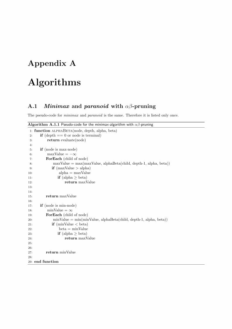
Appendix A
Algorithms
A.1 Minimax and paranoid with αβ-pruning
The pseudo-code for minimax and paranoid is the same. Therefore it is listed only once.
Algorithm A.1.1 Pseudo-code for the minimax-algorithm with αβ-pruning
1: function alphaBeta(node, depth, alpha, beta)2: if (depth == 0 or node is terminal)3: return evaluate(node)4:
5: if (node is max-node)6: maxValue = −∞7: ForEach (child of node)8: maxValue = max(maxValue, alphaBeta(child, depth-1, alpha, beta))9: if (maxValue > alpha)
10: alpha = maxValue11: if (alpha ≥ beta)12: return maxValue13:
14:
15: return maxValue16:
17: if (node is min-node)18: minValue = ∞19: ForEach (child of node)20: minValue = min(minValue, alphaBeta(child, depth-1, alpha, beta))21: if (minValue < beta)22: beta = minValue23: if (alpha ≥ beta)24: return maxValue25:
26:
27: return minValue28:
29: end function
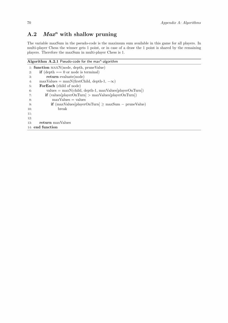
70 Appendix A: Algorithms
A.2 Maxn with shallow pruning
The variable maxSum in the pseudo-code is the maximum sum available in this game for all players. Inmulti-player Chess the winner gets 1 point, or in case of a draw the 1 point is shared by the remainingplayers. Therefore the maxSum in multi-player Chess is 1.
Algorithm A.2.1 Pseudo-code for the maxn-algorithm
1: function maxN(node, depth, pruneValue)2: if (depth == 0 or node is terminal)3: return evaluate(node)4: maxValues = maxN(firstChild, depth-1, −∞)5: ForEach (child of node)6: values = maxN(child, depth-1, maxValues[playerOnTurn])7: if (values[playerOnTurn] > maxValues[playerOnTurn])8: maxValues = values9: if (maxValues[playerOnTurn] ≥ maxSum − pruneValue)
10: break11:
12:
13: return maxValues14: end function
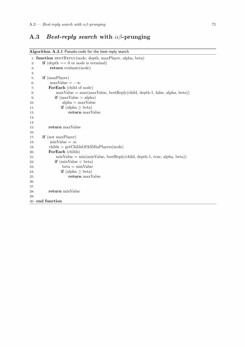
A.3 — Best-reply search with αβ-prunging 71
A.3 Best-reply search with αβ-prunging
Algorithm A.3.1 Pseudo-code for the best-reply search
1: function bestReply(node, depth, maxPlayer, alpha, beta)2: if (depth == 0 or node is terminal)3: return evaluate(node)4:
5: if (maxPlayer)6: maxValue = −∞7: ForEach (child of node)8: maxValue = max(maxValue, bestReply(child, depth-1, false, alpha, beta))9: if (maxValue > alpha)
10: alpha = maxValue11: if (alpha ≥ beta)12: return maxValue13:
14:
15: return maxValue16:
17: if (not maxPlayer)18: minValue = ∞19: childs = getChildsOfAllMinPlayers(node)20: ForEach (childs)21: minValue = min(minValue, bestReply(child, depth-1, true, alpha, beta))22: if (minValue < beta)23: beta = minValue24: if (alpha ≥ beta)25: return maxValue26:
27:
28: return minValue29:
30: end function