Embed Size (px)
Citation preview
Markov Decision Processes
Robert PlattNortheastern University
Some images and slides are used from:1. CS188 UC Berkeley2. RN, AIMA
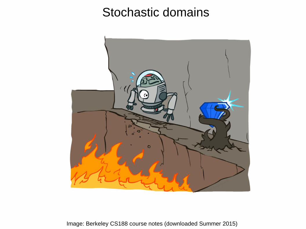
Stochastic domains
Image: Berkeley CS188 course notes (downloaded Summer 2015)

Example: stochastic grid world
Slide: based on Berkeley CS188 course notes (downloaded Summer 2015)
A maze-like problem The agent lives in a grid Walls block the agent’s path
Noisy movement: actions do not always go as planned 80% of the time, the action North takes the
agent North (if there is no wall there)
10% of the time, North takes the agent West; 10% East
If there is a wall in the direction the agent would have been taken, the agent stays put
The agent receives rewards each time step Reward function can be anything. For ex:
● Small “living” reward each step (can be negative)
● Big rewards come at the end (good or bad)
Goal: maximize (discounted) sum of rewards
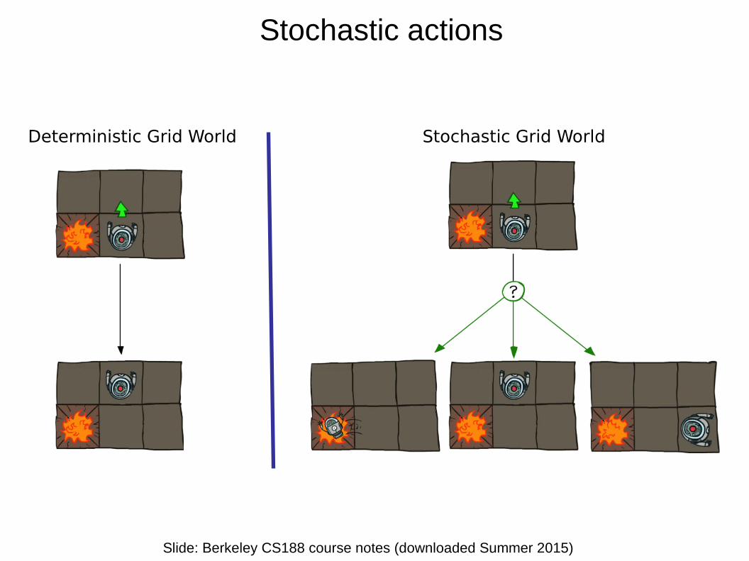
Stochastic actions
Slide: Berkeley CS188 course notes (downloaded Summer 2015)
Deterministic Grid World Stochastic Grid World
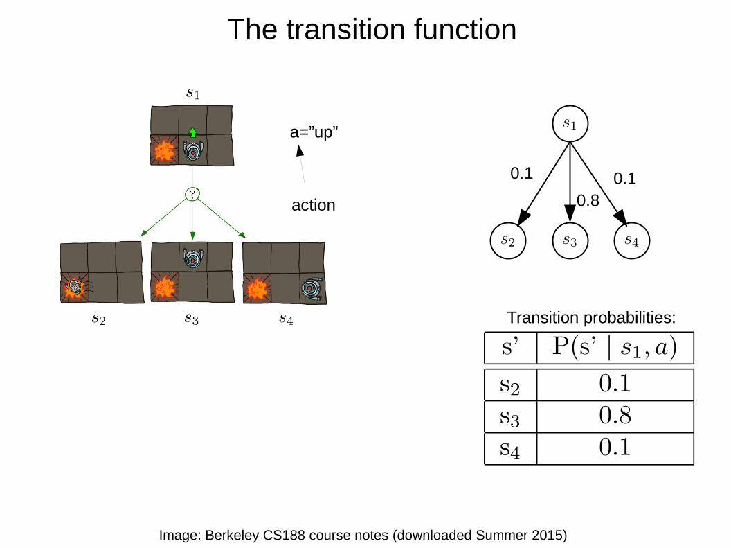
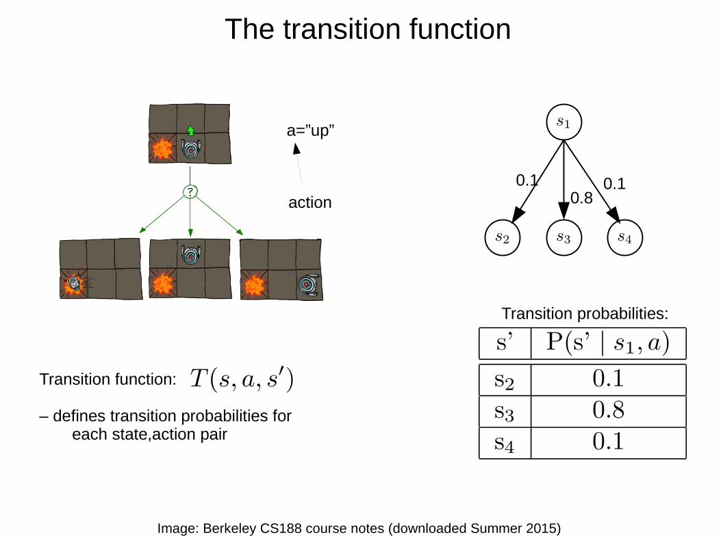
The transition function
Image: Berkeley CS188 course notes (downloaded Summer 2015)
0.80.10.1
a=”up”
action
Transition probabilities:
The transition function
Image: Berkeley CS188 course notes (downloaded Summer 2015)
0.80.10.1
a=”up”
action
Transition function:
– defines transition probabilities for each state,action pair
Transition probabilities:

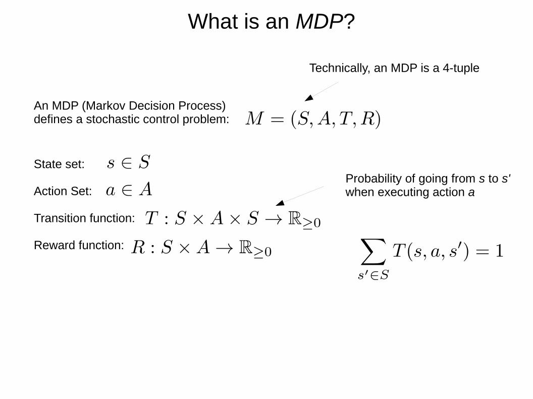
What is an MDP?
State set:
Action Set:
Transition function:
Reward function:
An MDP (Markov Decision Process) defines a stochastic control problem:
Technically, an MDP is a 4-tuple
What is an MDP?
State set:
Action Set:
Transition function:
Reward function:
An MDP (Markov Decision Process) defines a stochastic control problem:
Probability of going from s to s' when executing action a
Technically, an MDP is a 4-tuple
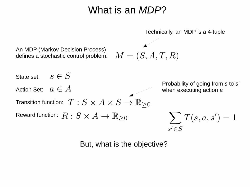
What is an MDP?
State set:
Action Set:
Transition function:
Reward function:
An MDP (Markov Decision Process) defines a stochastic control problem:
Probability of going from s to s' when executing action a
Technically, an MDP is a 4-tuple
But, what is the objective?
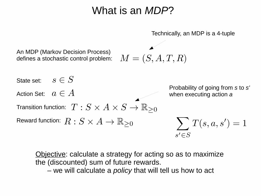
What is an MDP?
State set:
Action Set:
Transition function:
Reward function:
An MDP (Markov Decision Process) defines a stochastic control problem:
Probability of going from s to s' when executing action a
Objective: calculate a strategy for acting so as to maximize the (discounted) sum of future rewards.
– we will calculate a policy that will tell us how to act
Technically, an MDP is a 4-tuple
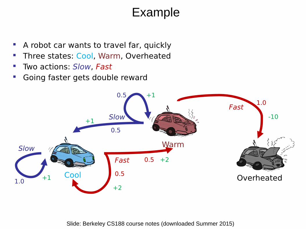
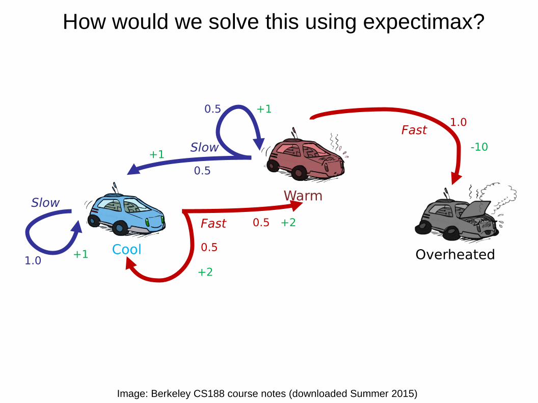
Example
Slide: Berkeley CS188 course notes (downloaded Summer 2015)
A robot car wants to travel far, quickly Three states: Cool, Warm, Overheated Two actions: Slow, Fast Going faster gets double reward
Cool
Warm
Overheated
Fast
Fast
Slow
Slow
0.5
0.5
0.5
0.5
1.0
1.0
+1
+1
+1
+2
+2
-10
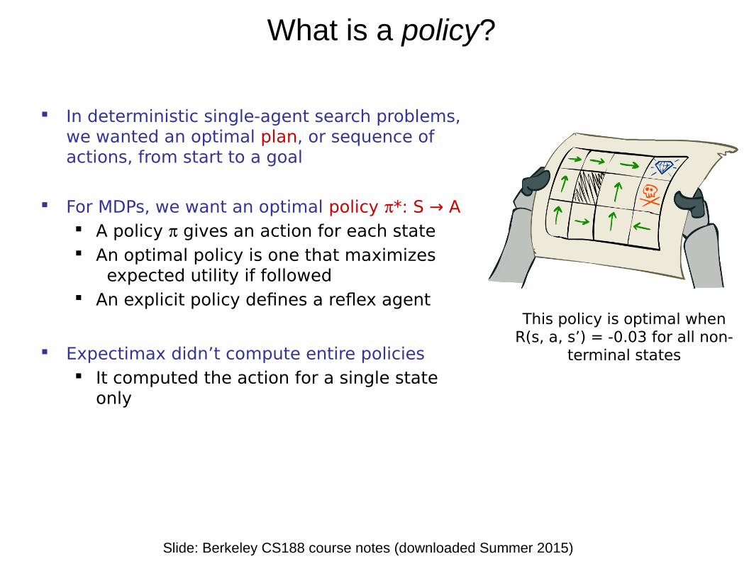
What is a policy?
Slide: Berkeley CS188 course notes (downloaded Summer 2015)
This policy is optimal when R(s, a, s’) = -0.03 for all non-
terminal states
In deterministic single-agent search problems, we wanted an optimal plan, or sequence of actions, from start to a goal
For MDPs, we want an optimal policy *: S → A A policy gives an action for each state An optimal policy is one that maximizes
expected utility if followed An explicit policy defines a reflex agent
Expectimax didn’t compute entire policies It computed the action for a single state
only
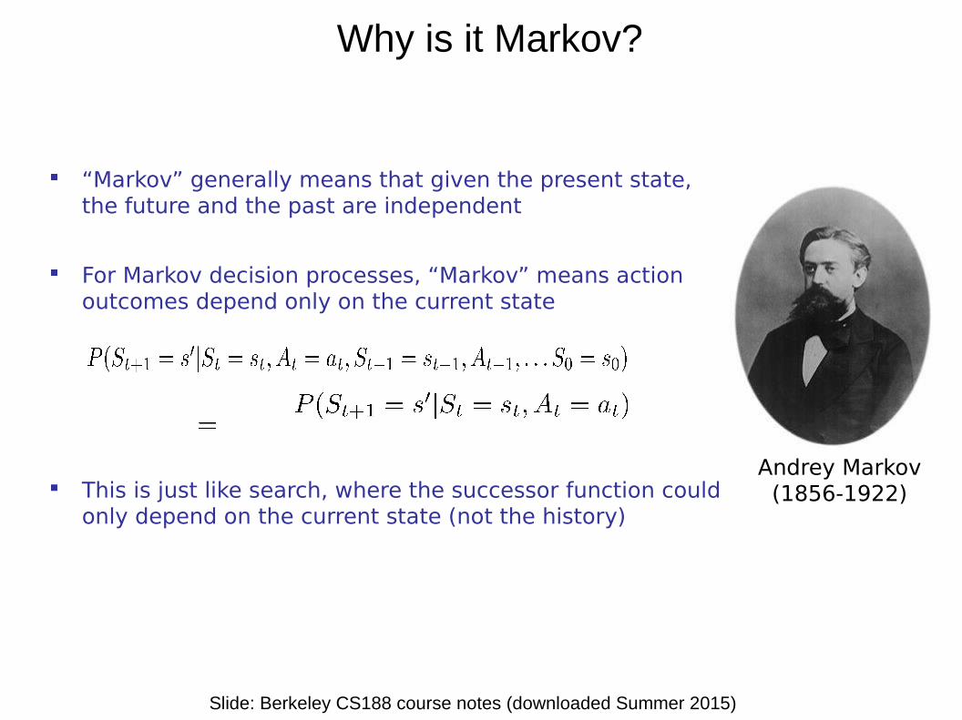
Why is it Markov?
Slide: Berkeley CS188 course notes (downloaded Summer 2015)
“Markov” generally means that given the present state, the future and the past are independent
For Markov decision processes, “Markov” means action outcomes depend only on the current state
This is just like search, where the successor function could only depend on the current state (not the history)
Andrey Markov (1856-1922)
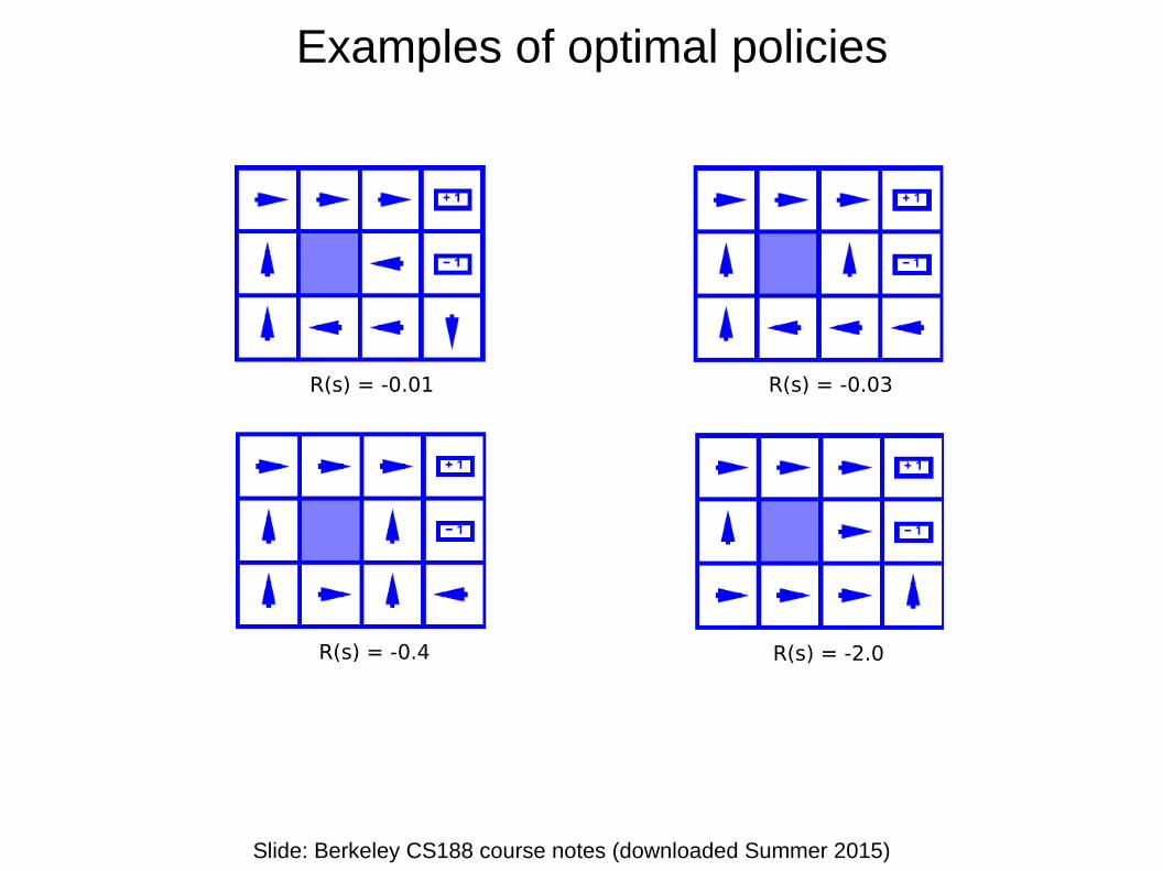
Examples of optimal policies
Slide: Berkeley CS188 course notes (downloaded Summer 2015)
R(s) = -2.0R(s) = -0.4
R(s) = -0.03R(s) = -0.01
How would we solve this using expectimax?
Image: Berkeley CS188 course notes (downloaded Summer 2015)
Cool
Warm
Overheated
Fast
Fast
Slow
Slow
0.5
0.5
0.5
0.5
1.0
1.0
+1
+1
+1
+2
+2
-10
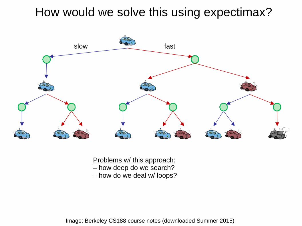
How would we solve this using expectimax?
Image: Berkeley CS188 course notes (downloaded Summer 2015)
slow fast
Problems w/ this approach:– how deep do we search?– how do we deal w/ loops?
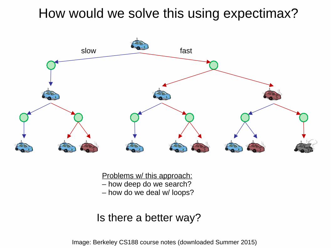
How would we solve this using expectimax?
Image: Berkeley CS188 course notes (downloaded Summer 2015)
slow fast
Problems w/ this approach:– how deep do we search?– how do we deal w/ loops?
Is there a better way?
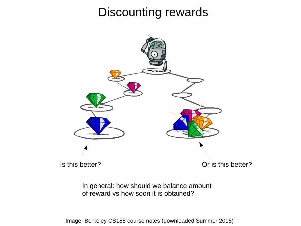
Discounting rewards
Image: Berkeley CS188 course notes (downloaded Summer 2015)
Is this better? Or is this better?
In general: how should we balance amount of reward vs how soon it is obtained?
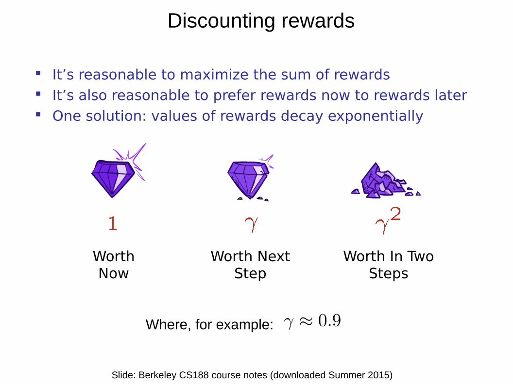
Discounting rewards
Slide: Berkeley CS188 course notes (downloaded Summer 2015)
It’s reasonable to maximize the sum of rewards It’s also reasonable to prefer rewards now to rewards later One solution: values of rewards decay exponentially
Worth Now
Worth Next Step
Worth In Two Steps
Where, for example:
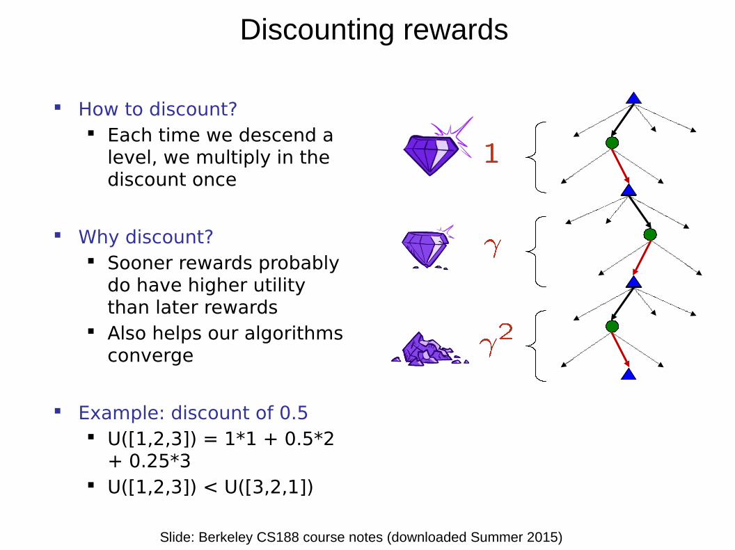
Discounting rewards
Slide: Berkeley CS188 course notes (downloaded Summer 2015)
How to discount? Each time we descend a
level, we multiply in the discount once
Why discount? Sooner rewards probably
do have higher utility than later rewards
Also helps our algorithms converge
Example: discount of 0.5 U([1,2,3]) = 1*1 + 0.5*2
+ 0.25*3 U([1,2,3]) < U([3,2,1])
Discounting rewards
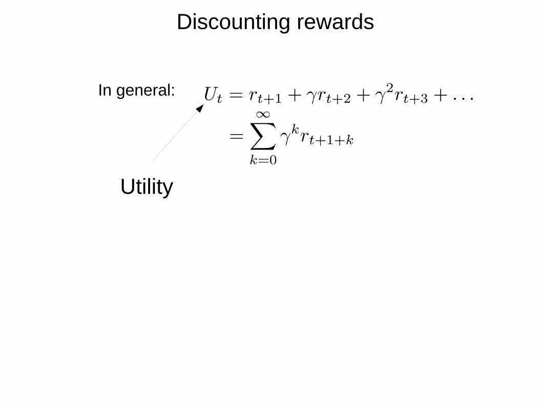
In general:
Utility
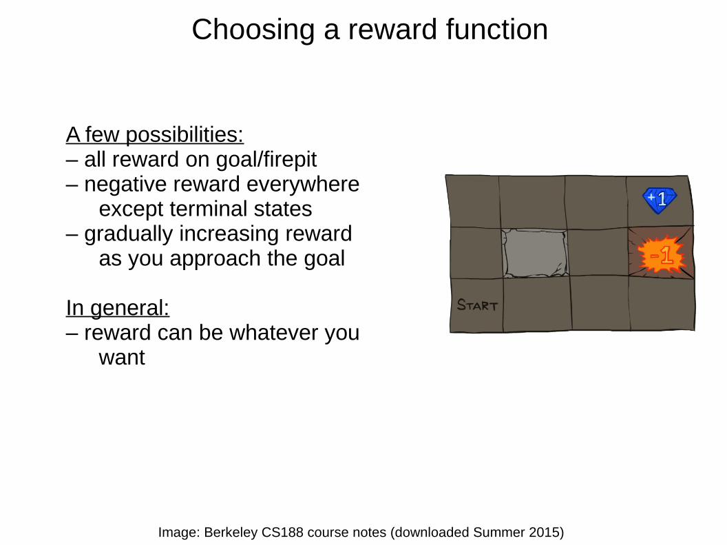
Choosing a reward function
Image: Berkeley CS188 course notes (downloaded Summer 2015)
A few possibilities:– all reward on goal/firepit– negative reward everywhere
except terminal states– gradually increasing reward
as you approach the goal
In general:– reward can be whatever you
want
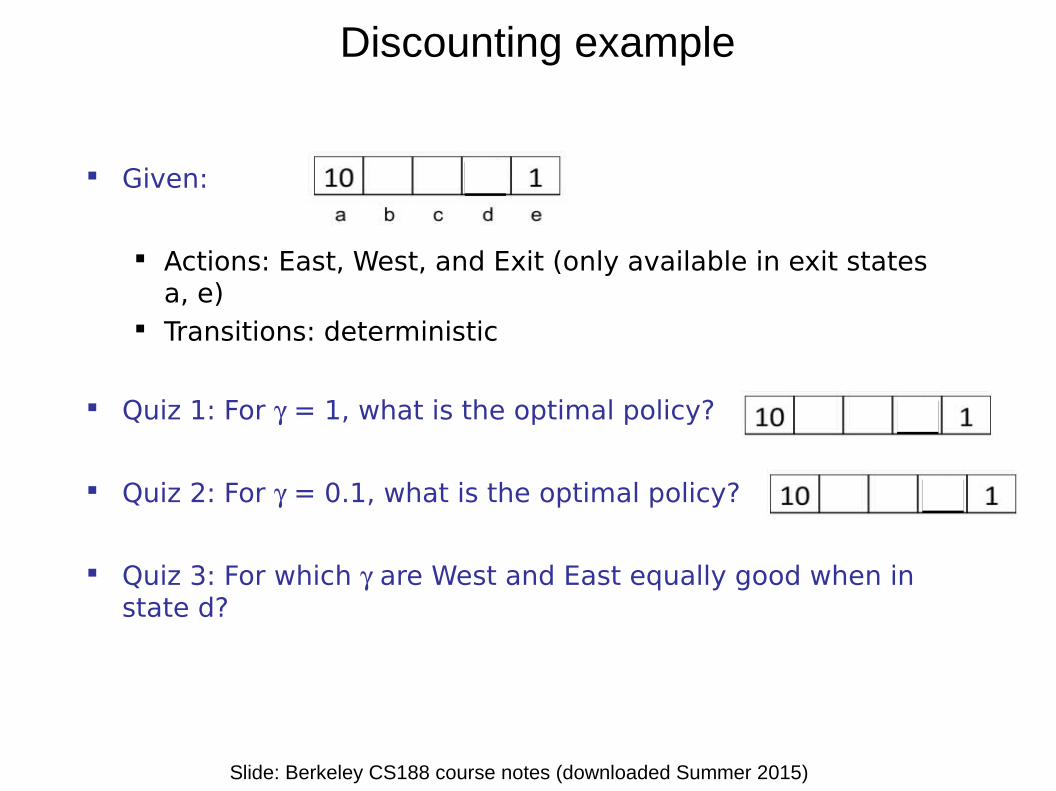
Discounting example
Slide: Berkeley CS188 course notes (downloaded Summer 2015)
Given:
Actions: East, West, and Exit (only available in exit states a, e)
Transitions: deterministic
Quiz 1: For = 1, what is the optimal policy?
Quiz 2: For = 0.1, what is the optimal policy?
Quiz 3: For which are West and East equally good when in state d?
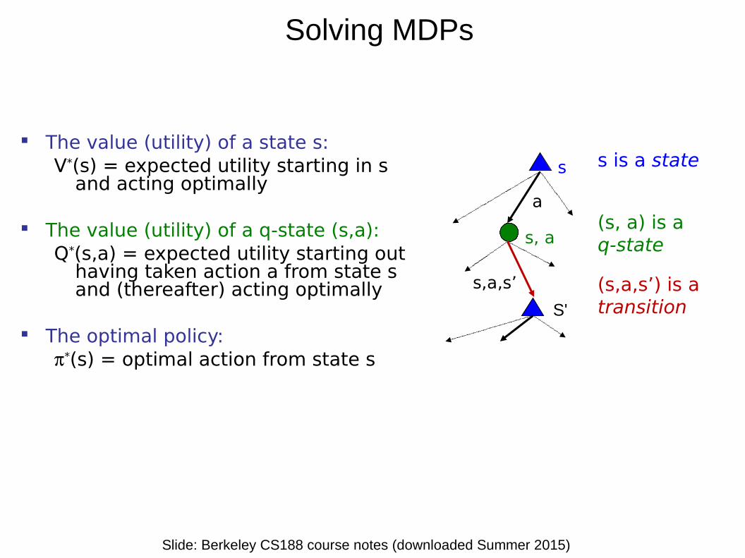
Solving MDPs
Slide: Berkeley CS188 course notes (downloaded Summer 2015)
The value (utility) of a state s:V*(s) = expected utility starting in s
and acting optimally
The value (utility) of a q-state (s,a):Q*(s,a) = expected utility starting out
having taken action a from state s and (thereafter) acting optimally
The optimal policy:*(s) = optimal action from state s
a
s
s, a
(s,a,s’) is a transition
s,a,s’
s is a state
(s, a) is a q-state
S'

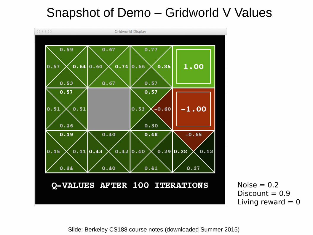
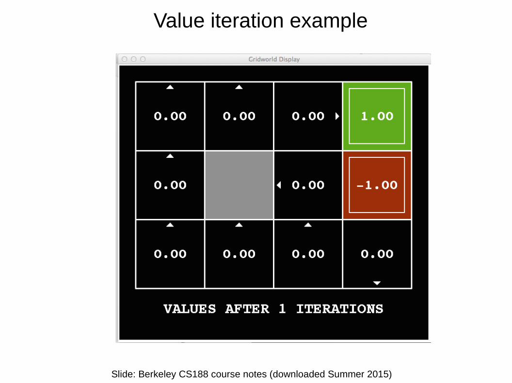
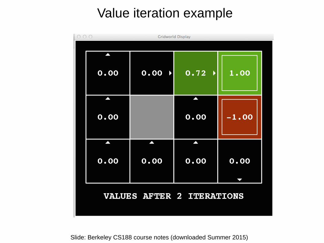
Snapshot of Demo – Gridworld V Values
Slide: Berkeley CS188 course notes (downloaded Summer 2015)
Noise = 0.2Discount = 0.9Living reward = 0
Snapshot of Demo – Gridworld V Values
Slide: Berkeley CS188 course notes (downloaded Summer 2015)
Noise = 0.2Discount = 0.9Living reward = 0
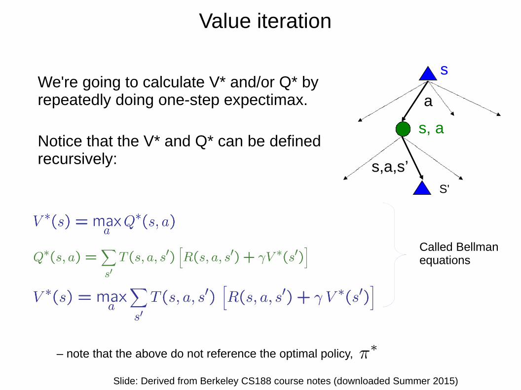
Value iteration
Slide: Derived from Berkeley CS188 course notes (downloaded Summer 2015)
a
s
s, a
s,a,s’
We're going to calculate V* and/or Q* by repeatedly doing one-step expectimax.
Notice that the V* and Q* can be defined recursively:
Called Bellman equations
S'
– note that the above do not reference the optimal policy,
Value iteration
Image: Berkeley CS188 course notes (downloaded Summer 2015)
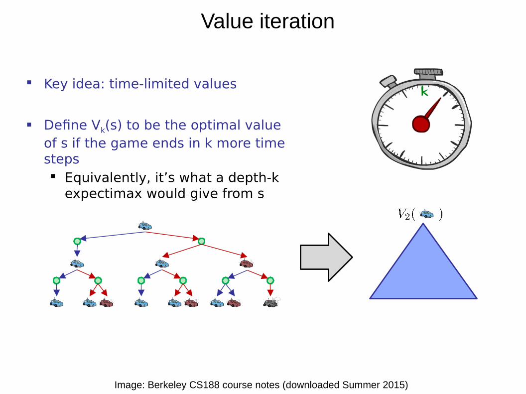
Key idea: time-limited values
Define Vk(s) to be the optimal value of s if the game ends in k more time steps Equivalently, it’s what a depth-k
expectimax would give from s

Value iteration
Image: Berkeley CS188 course notes (downloaded Summer 2015)
a
Vk+1(s)
s, a
s,a,s’
Vk(s’)
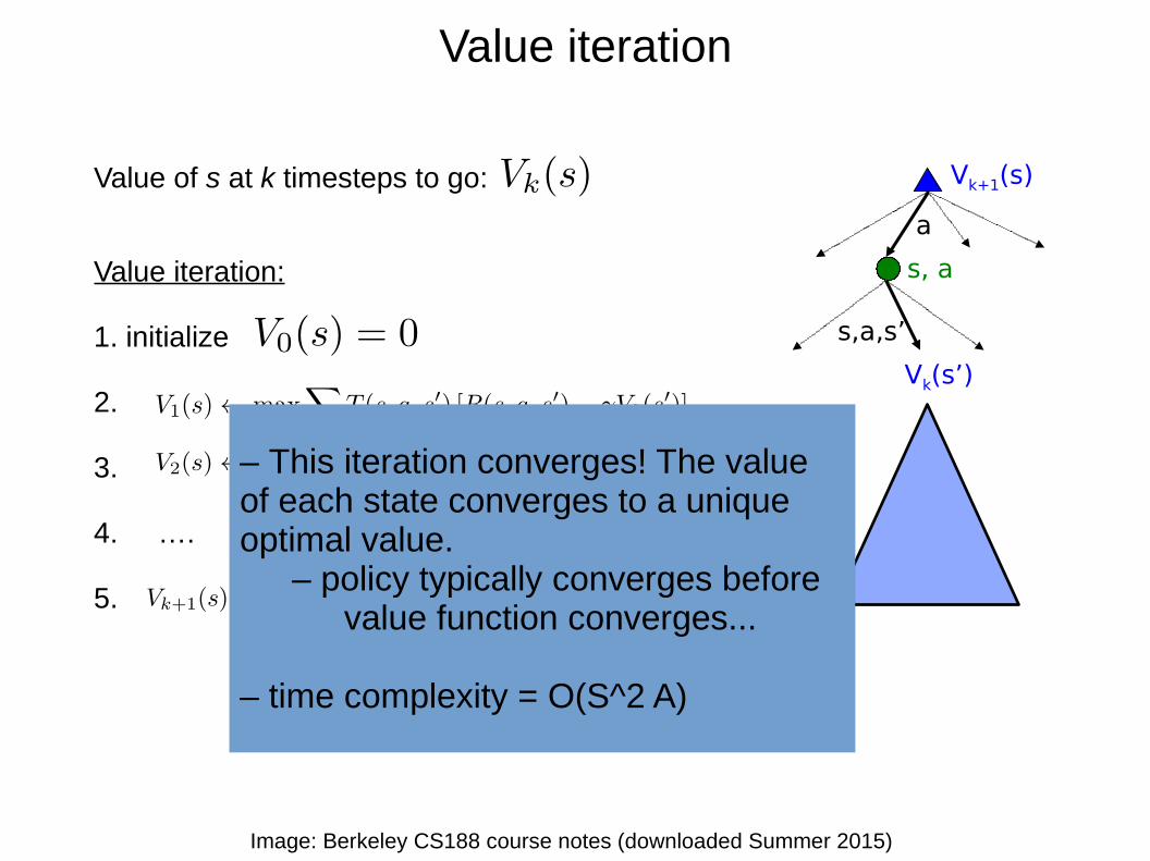
Value of s at k timesteps to go:
Value iteration:
1. initialize
2.
3.
4. ….
5.
Value iteration
Image: Berkeley CS188 course notes (downloaded Summer 2015)
a
Vk+1(s)
s, a
s,a,s’
Vk(s’)
Value of s at k timesteps to go:
Value iteration:
1. initialize
2.
3.
4. ….
5.
– This iteration converges! The value of each state converges to a unique optimal value.
– policy typically converges beforevalue function converges...
– time complexity = O(S^2 A)
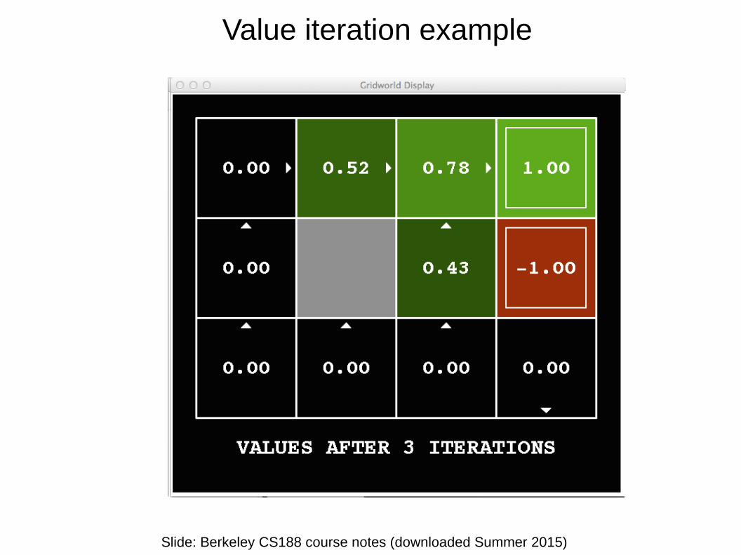
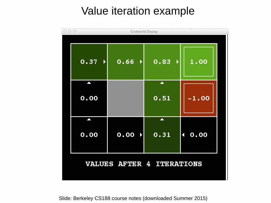
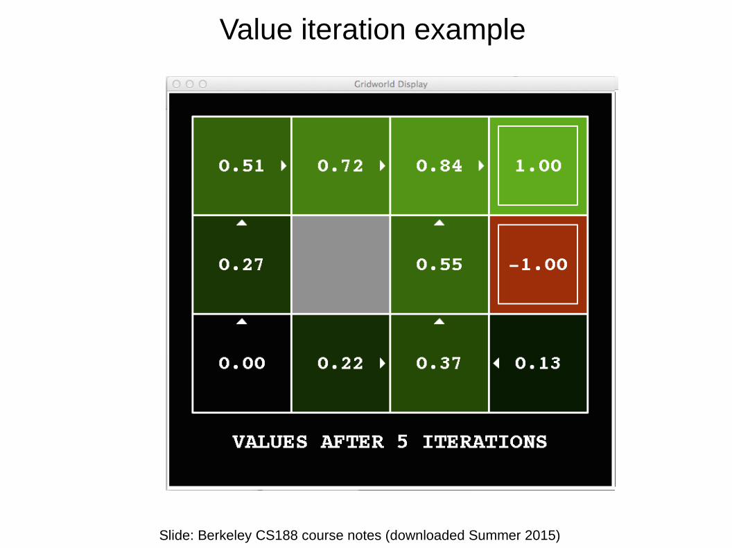
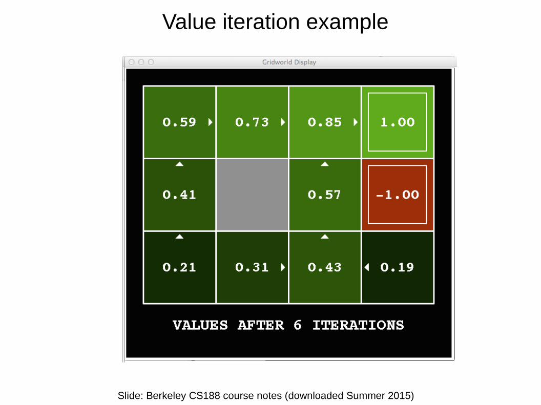
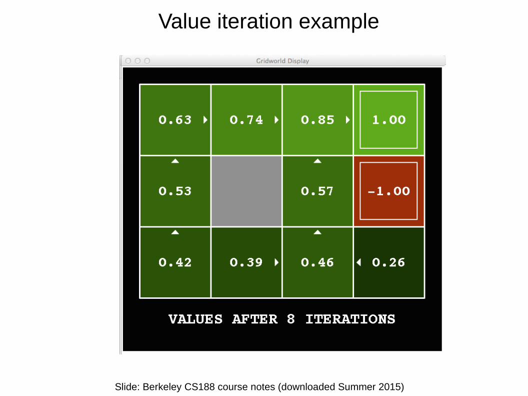
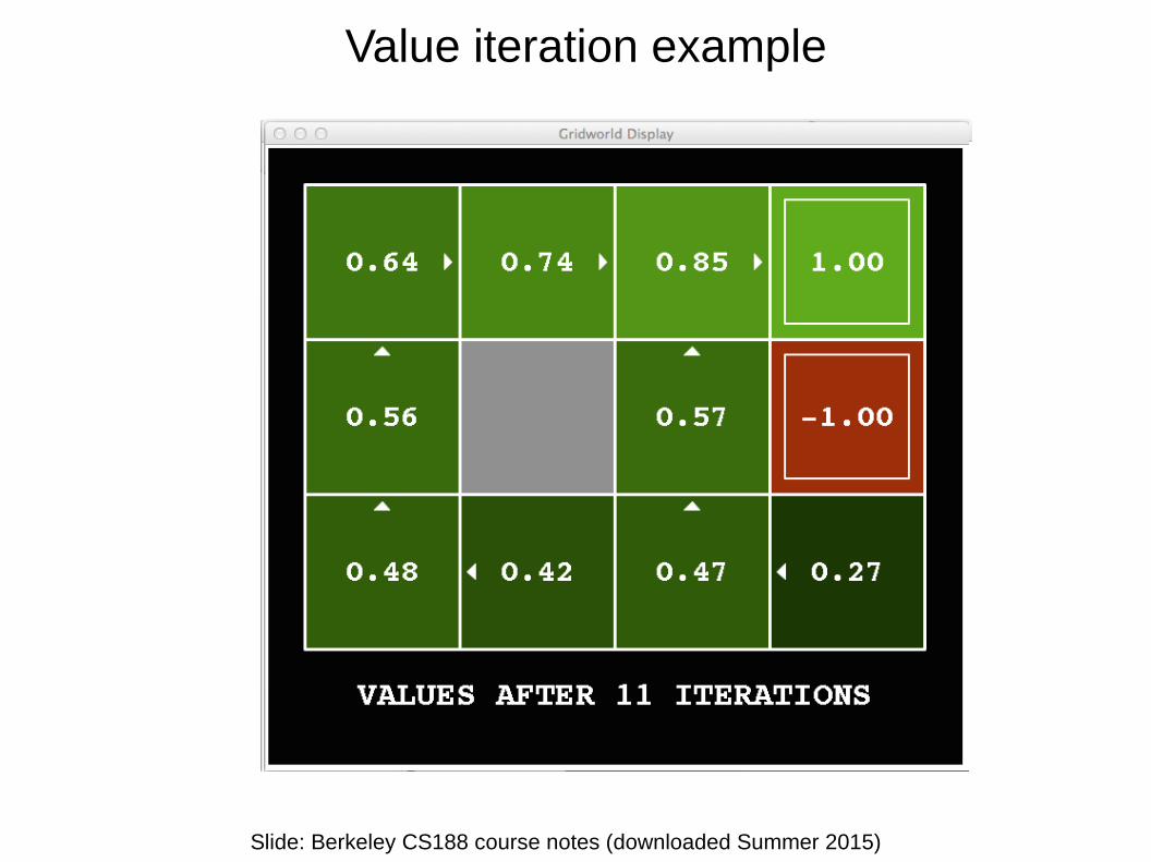
Value iteration example
Slide: Berkeley CS188 course notes (downloaded Summer 2015)
0 0 0
Assume no discount
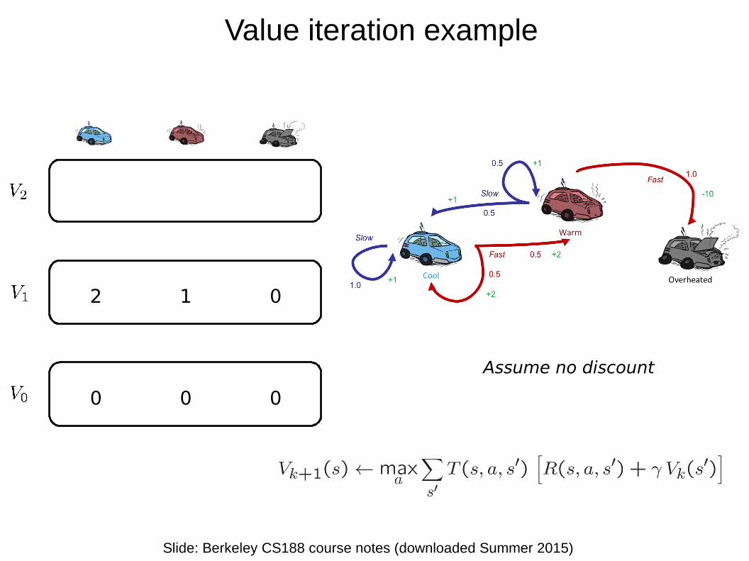
Value iteration example
Slide: Berkeley CS188 course notes (downloaded Summer 2015)
0 0 0
2 1 0
Assume no discount
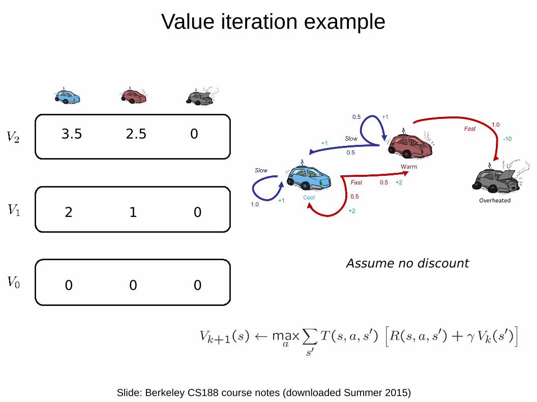
Value iteration example
Slide: Berkeley CS188 course notes (downloaded Summer 2015)
0 0 0
2 1 0
3.5 2.5 0
Assume no discount
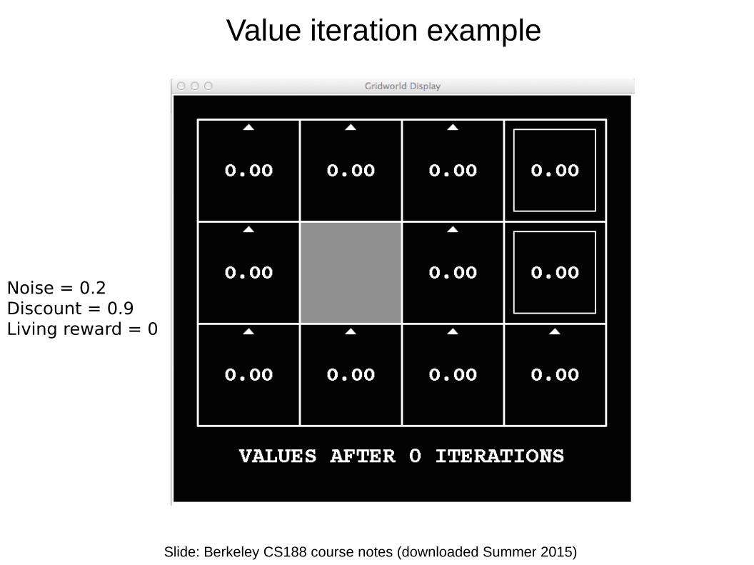
Value iteration example
Slide: Berkeley CS188 course notes (downloaded Summer 2015)
Noise = 0.2Discount = 0.9Living reward = 0
Value iteration example
Slide: Berkeley CS188 course notes (downloaded Summer 2015)
Value iteration example
Slide: Berkeley CS188 course notes (downloaded Summer 2015)
Value iteration example
Slide: Berkeley CS188 course notes (downloaded Summer 2015)
Value iteration example
Slide: Berkeley CS188 course notes (downloaded Summer 2015)
Value iteration example
Slide: Berkeley CS188 course notes (downloaded Summer 2015)
Value iteration example
Slide: Berkeley CS188 course notes (downloaded Summer 2015)

Value iteration example
Slide: Berkeley CS188 course notes (downloaded Summer 2015)
Value iteration example
Slide: Berkeley CS188 course notes (downloaded Summer 2015)

Value iteration example
Slide: Berkeley CS188 course notes (downloaded Summer 2015)

Value iteration example
Slide: Berkeley CS188 course notes (downloaded Summer 2015)
Value iteration example
Slide: Berkeley CS188 course notes (downloaded Summer 2015)

Value iteration example
Slide: Berkeley CS188 course notes (downloaded Summer 2015)

Value iteration example
Slide: Berkeley CS188 course notes (downloaded Summer 2015)
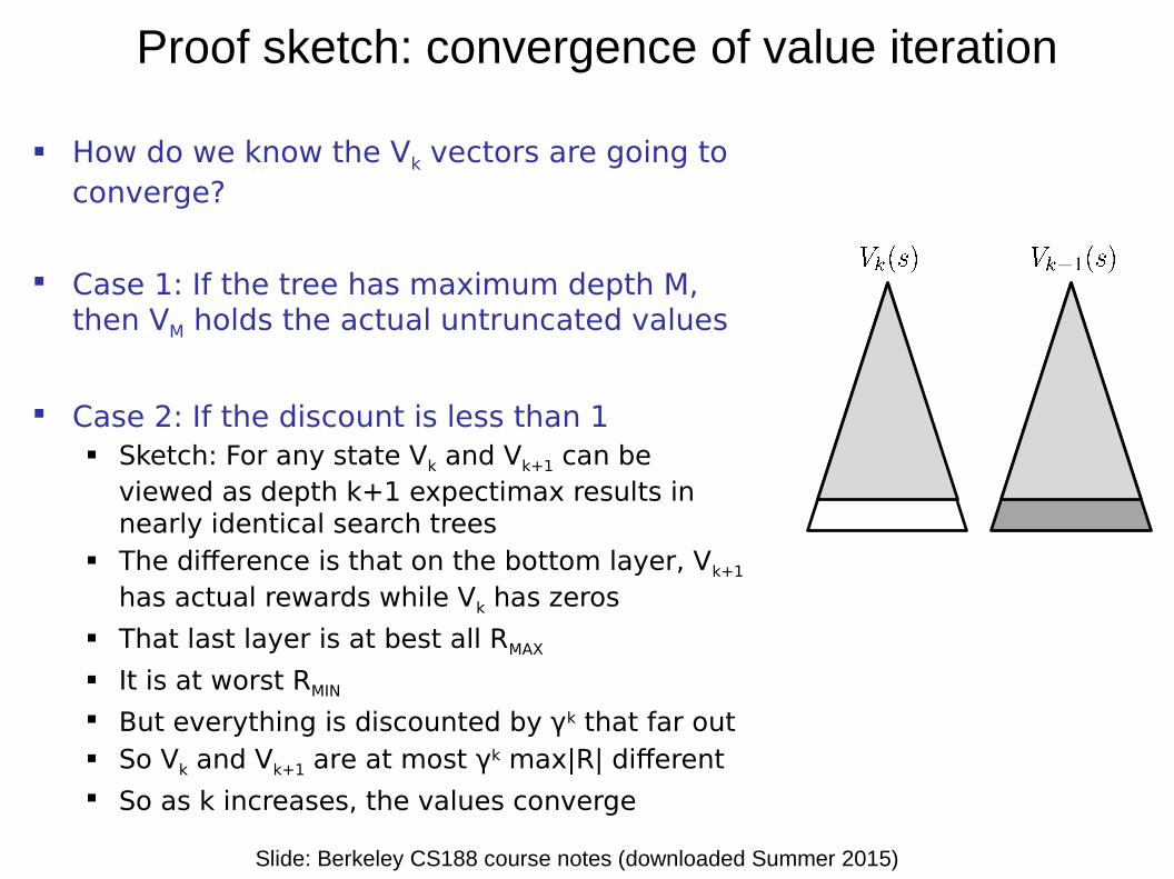
Proof sketch: convergence of value iteration
Slide: Berkeley CS188 course notes (downloaded Summer 2015)
How do we know the Vk vectors are going to converge?
Case 1: If the tree has maximum depth M, then VM holds the actual untruncated values
Case 2: If the discount is less than 1 Sketch: For any state Vk and Vk+1 can be
viewed as depth k+1 expectimax results in nearly identical search trees
The difference is that on the bottom layer, Vk+1 has actual rewards while Vk has zeros
That last layer is at best all RMAX
It is at worst RMIN
But everything is discounted by γk that far out So Vk and Vk+1 are at most γk max|R| different
So as k increases, the values converge
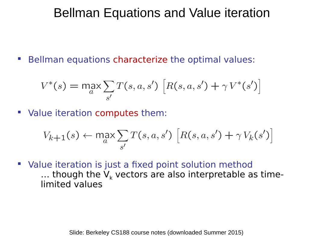
Bellman Equations and Value iteration
Slide: Berkeley CS188 course notes (downloaded Summer 2015)
Bellman equations characterize the optimal values:
Value iteration computes them:
Value iteration is just a fixed point solution method… though the Vk vectors are also interpretable as time-limited values
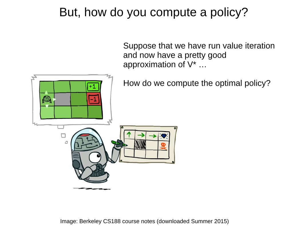
But, how do you compute a policy?
Suppose that we have run value iteration and now have a pretty good approximation of V* …
How do we compute the optimal policy?
Image: Berkeley CS188 course notes (downloaded Summer 2015)
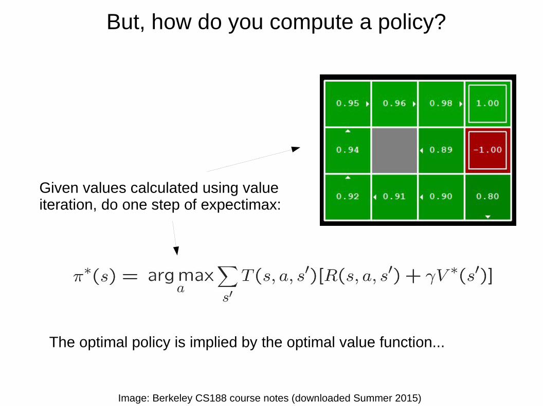
But, how do you compute a policy?
Given values calculated using value iteration, do one step of expectimax:
Image: Berkeley CS188 course notes (downloaded Summer 2015)
The optimal policy is implied by the optimal value function...