Embed Size (px)
Citation preview

Time-Dependence in
Markovian Decision Processes
Jeremy James McMahon
Thesis submitted for the degree of
Doctor of Philosophy
in
Applied Mathematics
at
The University of Adelaide
(Faculty of Mathematical and Computer Sciences)
School of Applied Mathematics
September, 2008

This work contains no material which has been accepted for the award of any other
degree or diploma in any university or other tertiary institution and, to the best of
my knowledge and belief, contains no material previously published or written by
another person, except where due reference has been made in the text.
I consent to this copy of my thesis, when deposited in the University Library, being
made available in all forms of media, now or hereafter known.
SIGNED: ....................... DATE: .......................

I extend sincere gratitude to my two supervisors, Professor Nigel Bean and Professor
Michael Rumsewicz, who have both inspired and guided me to complete this work.
Their input and encouragement has been extremely beneficial and I thank them
wholeheartedly for their friendship and support over the last few years.
I am grateful to all three of my parents for the love and reassurance they have given
me, not just throughout my time as a PhD student. Without them, any hope of
reaching this point in my education would at best be a distant dream. I particularly
appreciate the editorial contributions of my mother who, despite supposedly limited
mathematical knowledge, provided invaluable feedback.
Lastly, I thank my beautiful wife who has endured much whilst I have been working
on this thesis. I love and cherish Sarah for being by my side, encouraging me and
always believing in me. Now we may begin the next chapter of our lives.

For Olive.

Contents
Abstract xv
1 Introduction 1
2 Markov Processes 7
2.1 Introduction . . . . . . . . . . . . . . . . . . . . . . . . . . . . . . . . 7
2.2 A Markov Process . . . . . . . . . . . . . . . . . . . . . . . . . . . . . 8
2.2.1 The Markovian Assumption . . . . . . . . . . . . . . . . . . . 9
2.2.2 Time-Homogeneity . . . . . . . . . . . . . . . . . . . . . . . . 10
2.2.3 Analysis of Discrete-Time Markov Processes . . . . . . . . . . 10
2.2.4 Analysis of Continuous-Time Markov Processes . . . . . . . . 11
2.2.5 Discretizing Via Uniformization . . . . . . . . . . . . . . . . . 14
2.2.6 Applications . . . . . . . . . . . . . . . . . . . . . . . . . . . . 16
2.3 A Markov Decision Process . . . . . . . . . . . . . . . . . . . . . . . 19
2.3.1 Rewards and Decisions . . . . . . . . . . . . . . . . . . . . . . 20
2.3.2 Finite Horizon . . . . . . . . . . . . . . . . . . . . . . . . . . . 22
2.3.3 Infinite Horizon . . . . . . . . . . . . . . . . . . . . . . . . . . 25
2.3.4 Continuous Time . . . . . . . . . . . . . . . . . . . . . . . . . 27
2.4 A Semi-Markov Decision Process . . . . . . . . . . . . . . . . . . . . 30
2.5 A Generalized Semi-Markov Decision Process . . . . . . . . . . . . . 33
3 Phase-Type Distributions 37
3.1 Introduction . . . . . . . . . . . . . . . . . . . . . . . . . . . . . . . . 37
3.2 Phase-Type Representations . . . . . . . . . . . . . . . . . . . . . . . 38
vii

3.3 Using Phase-Type Distributions . . . . . . . . . . . . . . . . . . . . . 42
4 The Race 45
4.1 Introduction . . . . . . . . . . . . . . . . . . . . . . . . . . . . . . . . 45
4.2 The Race – Formal Description . . . . . . . . . . . . . . . . . . . . . 47
4.3 Restricted Vision . . . . . . . . . . . . . . . . . . . . . . . . . . . . . 49
4.3.1 Blind . . . . . . . . . . . . . . . . . . . . . . . . . . . . . . . . 49
4.3.2 Partially Observable . . . . . . . . . . . . . . . . . . . . . . . 53
4.4 Full Vision . . . . . . . . . . . . . . . . . . . . . . . . . . . . . . . . . 59
4.4.1 Value Equations . . . . . . . . . . . . . . . . . . . . . . . . . . 60
4.4.2 Policy Evaluation . . . . . . . . . . . . . . . . . . . . . . . . . 62
4.4.3 The Race Revisited . . . . . . . . . . . . . . . . . . . . . . . . 64
4.5 The Race – Exponential System . . . . . . . . . . . . . . . . . . . . . 67
4.5.1 Value Equations . . . . . . . . . . . . . . . . . . . . . . . . . . 68
4.5.2 MDP Approach . . . . . . . . . . . . . . . . . . . . . . . . . . 70
5 The Race – Erlang System 75
5.1 Introduction . . . . . . . . . . . . . . . . . . . . . . . . . . . . . . . . 75
5.2 Value Equations . . . . . . . . . . . . . . . . . . . . . . . . . . . . . . 77
5.2.1 State K . . . . . . . . . . . . . . . . . . . . . . . . . . . . . . 78
5.2.2 State K − 1 . . . . . . . . . . . . . . . . . . . . . . . . . . . . 79
5.2.3 State K − 2 . . . . . . . . . . . . . . . . . . . . . . . . . . . . 87
5.3 Summary . . . . . . . . . . . . . . . . . . . . . . . . . . . . . . . . . 91
6 Phase-Space Model – Erlang System 95
6.1 Introduction . . . . . . . . . . . . . . . . . . . . . . . . . . . . . . . . 95
6.2 Existing Phase-Space Techniques . . . . . . . . . . . . . . . . . . . . 100
6.3 Our Phase-Space Technique . . . . . . . . . . . . . . . . . . . . . . . 108
6.3.1 Level K . . . . . . . . . . . . . . . . . . . . . . . . . . . . . . 111
6.3.2 Level K − 1 . . . . . . . . . . . . . . . . . . . . . . . . . . . . 111
6.3.3 Level K − 2 . . . . . . . . . . . . . . . . . . . . . . . . . . . . 115
viii

6.3.4 Level K − 3 . . . . . . . . . . . . . . . . . . . . . . . . . . . . 123
6.4 Summary . . . . . . . . . . . . . . . . . . . . . . . . . . . . . . . . . 127
7 Phase-Space Model – General Analysis 131
7.1 The Decision Process and Optimal Actions . . . . . . . . . . . . . . . 131
7.2 Phase-Space Construction . . . . . . . . . . . . . . . . . . . . . . . . 133
7.3 Action-Consistent Valuation . . . . . . . . . . . . . . . . . . . . . . . 140
7.4 Optimality Equations . . . . . . . . . . . . . . . . . . . . . . . . . . . 144
7.5 Level-skipping in the Phase-Space . . . . . . . . . . . . . . . . . . . . 148
7.6 The Phase-Space Technique . . . . . . . . . . . . . . . . . . . . . . . 154
8 Time-Inhomogeneous MDPs 157
8.1 Introduction . . . . . . . . . . . . . . . . . . . . . . . . . . . . . . . . 157
8.2 Time-Inhomogeneous Discounting . . . . . . . . . . . . . . . . . . . . 159
8.3 The Random Time Clock Technique . . . . . . . . . . . . . . . . . . . 162
8.3.1 Time Representation . . . . . . . . . . . . . . . . . . . . . . . 163
8.3.2 State-Space Construction . . . . . . . . . . . . . . . . . . . . . 165
8.3.3 Reward Structure and Discounting . . . . . . . . . . . . . . . 168
8.3.4 Truncation . . . . . . . . . . . . . . . . . . . . . . . . . . . . . 171
8.3.5 Implementation . . . . . . . . . . . . . . . . . . . . . . . . . . 174
8.3.6 Extension for Time-Inhomogeneous Transitions . . . . . . . . 178
8.4 The Race – Erlang System . . . . . . . . . . . . . . . . . . . . . . . . 180
8.5 Summary . . . . . . . . . . . . . . . . . . . . . . . . . . . . . . . . . 192
9 Conclusions 195
References 199
ix

List of Figures
2.2.1 Example of a continuous-time Markov process . . . . . . . . . . . . . 17
2.5.1 State-space of the toast and tea example . . . . . . . . . . . . . . . . 35
3.1.1 Graphical representation of a selection of PH distributions . . . . . . 39
4.3.1 Optimal waiting time in state 2 given decision epoch at time s . . . . 52
4.3.2 Optimal expected value for state 2 at decision epoch s . . . . . . . . 57
4.3.3 Optimal expected value for state 1 at decision epoch s . . . . . . . . 58
4.3.4 Optimal expected value for state 0 at decision epoch s . . . . . . . . 59
4.5.1 Markov chain state-space of the exponential system . . . . . . . . . . 71
5.2.1 Expected value for state 2 at decision epoch s for differing actions . . 87
5.2.2 Optimal expected value for state 1 at decision epoch s . . . . . . . . 90
5.3.1 Optimal expected value for state 0 at decision epoch s . . . . . . . . 92
6.1.1 Markov chain representation of the Erlang order p distribution . . . . 96
6.1.2 Markov Chain representation of the K Erlang order 2 phase-space . . 98
6.2.1 Comparison of expected values for optimal and randomized policies . 102
6.2.2 Guideline summary of the phase tracking model . . . . . . . . . . . . 103
6.2.3 Comparison of techniques for state/level 1 . . . . . . . . . . . . . . . 106
6.2.4 Expected optimal value of level 2 as seen from level 1 . . . . . . . . . 107
6.3.1 Guideline summary of the phase-space technique . . . . . . . . . . . . 110
6.3.2 Continuation values in level 1 . . . . . . . . . . . . . . . . . . . . . . 121
6.3.3 Comparison of techniques for state/level 1 . . . . . . . . . . . . . . . 122
6.3.4 Comparison of techniques for state/level 0 . . . . . . . . . . . . . . . 126
xi

6.4.1 Algorithmic summary of the phase-space technique for the race . . . 129
7.2.1 A two state semi-Markov reward process . . . . . . . . . . . . . . . . 135
7.2.2 Phase-space of a two state semi-Markov reward process . . . . . . . . 136
7.5.1 Level-skipping of a (TD,NAC) level . . . . . . . . . . . . . . . . . . 151
7.5.2 Level-skipping of a (TD,AC) level . . . . . . . . . . . . . . . . . . . 151
7.5.3 Example of level-skipping in the phase-space technique . . . . . . . . 154
8.2.1 MOS decay as end-to-end delay is increased . . . . . . . . . . . . . . 160
8.3.1 State-space of a simple 2 state Markov process . . . . . . . . . . . . . 163
8.3.2 Erlang density function of mean 1 with differing parameters . . . . . 165
8.3.3 RTC State-space of a 2 state Markov process . . . . . . . . . . . . . . 167
8.3.4 Algorithmic summary of the RTC technique . . . . . . . . . . . . . . 177
8.3.5 RTC State-space of a 2 state time-inhomogeneous Markov process . . 179
8.4.1 Markov chain defined by Q0(t) . . . . . . . . . . . . . . . . . . . . . . 183
8.4.2 Markov chain defined by Q1(t) . . . . . . . . . . . . . . . . . . . . . . 183
8.4.3 Sigmoid absolute discount function . . . . . . . . . . . . . . . . . . . 184
8.4.4 RTC state-space and transition rates when continue is selected . . . . 186
8.4.5 RTC technique with various time-state resolutions . . . . . . . . . . . 188
8.4.6 Technique comparison for optimal value of state 2 . . . . . . . . . . . 190
8.4.7 Absolute error of the RTC technique for state 2 . . . . . . . . . . . . 191
8.4.8 Technique comparison for optimal value of state 1 . . . . . . . . . . . 192
xii

List of Tables
5.2.1 Summary of optimal policies . . . . . . . . . . . . . . . . . . . . . . . 85
6.1.1 Optimal values for phase-states in a K Erlang order 2 system . . . . 99
8.4.1 Termination rewards for the RTC state-space . . . . . . . . . . . . . 187
xiii
Abstract
The main focus of this thesis is Markovian decision processes with an emphasis on
incorporating time-dependence into the system dynamics. When considering such
decision processes, we provide value equations that apply to a large range of classes
of Markovian decision processes, including Markov decision processes (MDPs) and
semi-Markov decision processes (SMDPs), time-homogeneous or otherwise. We then
formulate a simple decision process with exponential state transitions and solve this
decision process using two separate techniques. The first technique solves the value
equations directly, and the second utilizes an existing continuous-time MDP solution
technique.
To incorporate time-dependence into the transition dynamics of the process,
we examine a particular decision process with state transitions determined by the
Erlang distribution. Although this process is originally classed as a generalized
semi-Markov decision process, we re-define it as a time-inhomogeneous SMDP. We
show that even for a simply stated process with desirable state-space properties,
the complexity of the value equations becomes so substantial that useful analytic
expressions for the optimal solutions for all states of the process are unattainable.
We develop a new technique, utilizing phase-type (PH ) distributions, in an effort
to address these complexity issues. By using PH representations, we construct a
new state-space for the process, referred to as the phase-space, incorporating the
phases of the state transition probability distributions. In performing this step, we
effectively model the original process as a continuous-time MDP. The information
available in this system is, however, richer than that of the original system. In the
interest of maintaining the physical characteristics of the original system, we define
xv

a new valuation technique for the phase-space that shields some of this information
from the decision maker. Using the process of phase-space construction and our
valuation technique, we define an original system of value equations for this phase-
space that are equivalent to those for the general Markovian decision processes
mentioned earlier. An example of our own phase-space technique is given for the
aforementioned Erlang decision process and we identify certain characteristics of the
optimal solution such that, when applicable, the implementation of our phase-space
technique is greatly simplified.
These newly defined value equations for the phase-space are potentially as com-
plex to solve as those defined for the original model. Restricting our focus to systems
with acyclic state-spaces though, we describe a top-down approach to solution of the
phase-space value equations for more general processes than those considered thus
far. Again, we identify characteristics of the optimal solution to look for when im-
plementing this technique and provide simplifications of the value equations where
these characteristics are present. We note, however, that it is almost impossible to
determine a priori the class of processes for which the simplifications outlined in our
phase-space technique will be applicable. Nevertheless, we do no worse in terms of
complexity by utilizing our phase-space technique, and leave open the opportunity
to simplify the solution process if an appropriate situation arises.
The phase-space technique can handle time-dependence in the state transition
probabilities, but is insufficient for any process with time-dependent reward struc-
tures or discounting. To address such decision processes, we define an approximation
technique for the solution of the class of infinite horizon decision processes whose
state transitions and reward structures are described with reference to a single global
clock. This technique discretizes time into exponentially distributed length intervals
and incorporates this absolute time information into the state-space. For processes
where the state-transitions are not exponentially distributed, we use the hazard rates
of the transition probability distributions evaluated at the discrete time points to
model the transition dynamics of the system. We provide a suitable reward structure
approximation using our discrete time points and guidelines for sensible truncation,
xvi

using an MDP approximation to the tail behaviour of the original infinite horizon
process. The result is a finite-state time-homogeneous MDP approximation to the
original process and this MDP may be solved using standard existing solution tech-
niques. The approximate solution to the original process can then be inferred from
the solution to our MDP approximation.
xvii
Chapter 1
Introduction
This thesis contains a study of various aspects of time-dependence in Markovian de-
cision processes. The inspiration for this work stemmed from a seemingly innocuous
problem studied from a simulation point of view in McMahon et al. [63]. The pro-
cess considered in [63] models an audio server whose job is to merge digitized audio
packets from a number of sources into a single audio packet. A fixed time-out at the
server was implemented for each set of audio packets, referred to as a frame, and the
process was studied from a failure recovery and quality of service perspective. At
the time-out for a given audio frame, only those audio packets present at the server
are included in the merged packet and those yet to arrive become associated with
the next audio frame. The question of an appropriate time-out value was, however,
not addressed in [63].
Consider the mathematically abstracted scenario where we have a set of particles
that we release toward a destination and then record their individual arrival times
at that destination. At any time after the release of the particles, we will have a
subset of the particles present at the destination. One area of interest here is that at
any point, rather than waiting until some fixed time-out, we may ask the question
whether or not it is worth waiting for any more of the particles to arrive. This
decision will of course depend on the reward we receive for having certain particles
present when we cease waiting.
Such a scenario is referred to as the race throughout this thesis. The difficulty
1
2 CHAPTER 1. INTRODUCTION
in answering the question of whether or not to wait for more particles depends
very strongly on the arrival distributions of the particles and the reward structure
associated with the process. The variety of arrival and reward structures applicable
for this process means that this simply posed problem can fit into different extensions
of Markovian decision processes.
Using the race as a point of focus, we consider a range of Markovian decision
processes where we incorporate time-dependence into various aspects of the corre-
sponding arrival and reward structures. In general, the inclusion of time-dependent
aspects in a decision process complicates existing solution techniques significantly, if
solution techniques are available at all. In this thesis, we attempt to provide insight
into the difficulties surrounding time-dependence in Markovian decision processes
and outline the lack of practical solution techniques for certain classes. Where pos-
sible, we provide our own solution techniques for these complex decision processes.
We stress however that this thesis does not contain a single universal solution
technique applicable for general Markovian decision processes. The two original
techniques, phase-space and random time clock (RTC), each apply to their own
specific class of decision processes and these classes can themselves be difficult to
characterize. In general, the techniques cannot be applied blindly to an arbitrary
process and one requires some modelling experience to implement them effectively.
We provide a brief introduction to these issues later in this chapter when we describe
the progression of the work in this thesis.
The major contribution of the work contained herein is thus not the tech-
niques themselves, but rather the thought processes required for their development.
Each technique deals with its own addition of complexity, over that of a standard
continuous-time Markov decision process (MDP), introduced by the inclusion of
certain time-dependent aspects. The phase-space technique draws on the theory
of phase-type (PH ) distributions to provide an original system of value equations
for semi-Markov decision processes (SMDPs). By exploiting the properties of PH
distributions, we define characteristics of an optimal solution to these value equa-
tions that, when present, reduce the complexity of solution of the value equations

3
greatly. On the other hand, the RTC technique is an approximation technique that
represents time using exponentially distributed intervals to provide absolute time in-
formation in the treatment of time-inhomogeneous MDPs. This technique effectively
models a suitable class of infinite horizon processes as standard finite-state MDPs,
on which the standard solution techniques may be implemented. In the following
sketch of the progression of this thesis, we hope to make it clear that a multitude
of existing Markov process analysis tools, along with some original concepts, have
been utilized in a novel way. These original techniques have been developed to make
headway into a field of solution techniques that is scarce in the current literature
due to complexity issues.
Chapter 2 provides the reader with sufficient background regarding the variants
of Markovian processes and decision processes required throughout this thesis. It
begins with a discussion of certain properties of Markov processes with a focus on
analysis and applications. It then follows the evolution of the decision process coun-
terparts beginning with discrete-time finite horizon processes introduced by Bellman
[12] and infinite horizon processes introduced by Howard [41]. Next, the extension
to continuous-time and SMDPs is discussed, using the semi-Markov process formal-
ism defined in Cinlar [21]. Lastly, the topic of generalized semi-Markov decision
processes (GSMDPs) is introduced, using the generalized semi-Markov process for-
malism defined in Glynn [36]. It is important to note that in the literature reviewed
in this chapter, the restriction of time-homogeneity, whether it be related to tran-
sition probabilities or reward structures, is rarely relaxed. The added complexity,
when incorporating time-dependence into one or more aspects of the process, can
make the application of existing solution techniques too difficult from a practical
perspective.
In Chapter 3, an introduction to PH distributions, as first described by Neuts
[66], is given. A PH random variable is defined as the time to absorption in a finite-
state absorbing Markov chain. PH distributions are hence a very versatile class of
distributions that are dense in the set of non-negative distributions and yet they
have a simple probabilistic interpretation. It is this probabilistic interpretation that

4 CHAPTER 1. INTRODUCTION
we exploit to help simplify the solution of some rather complicated processes in later
chapters of this thesis.
Chapter 4 formally introduces the class of decision processes referred to as the
race. Initially, instances of the race are considered and analyzed when information
regarding the particles present at the destination is restricted. This restriction suits
the problem of merging audio packets of McMahon et al. [63] where, for practi-
cal reasons, only a subset of the system information is available at any time. The
more interesting and complex scenario of full system information is then introduced.
Given the potential complexity of the class of processes to which the race in general
may belong, we use the value equations from Chapter 6 of Janssen and Manca [49].
As we generally require control over the processes we are interested in, we then
modify their value equations to incorporate decisions. The resulting value equa-
tions, while too complex in general to solve, apply to a large range of classes of
decision processes including MDPs and SMDPs, time-homogeneous or otherwise.
This chapter is concluded by formulating a simple race with particles arriving fol-
lowing exponential distributions. This decision process is solved using two separate
techniques, initially by considering the value equations directly and then by utilizing
an existing continuous-time MDP solution technique as outlined in Puterman [74].
The entirety of Chapter 5 is dedicated to the study of the race, with each particle
arriving following an Erlang distribution, via direct analysis of the value equations
described in the previous chapter. The Erlang race has been chosen for this analysis
for a number of reasons. By utilizing the Erlang distribution, we define a pro-
cess with time-dependent transition probabilities, which are of particular interest
in this thesis. The class to which this version of the race belongs is that of time-
inhomogeneous SMDPs, for which, to the author’s knowledge, no general solution
technique exists other than direct solution of the resulting value equations. We
show that even for a simply stated process with desirable state-space properties,
the complexity of the value equations becomes so substantial that useful analytic
expressions for the optimal solutions for all states of the process are unattainable.
In Chapter 6, an initial introduction to the phase-space model of a process is

5
provided by considering the Erlang race of the previous chapter. By utilizing the
PH representation of the Erlang distribution we construct a new state-space for
the process, referred to as the phase-space, incorporating the phases of the state
transition probability distributions. In performing this step, we have effectively
modelled the state-space of the original process as a continuous-time Markov process.
One must nevertheless be cautious when valuing the states of the phase-space as the
phases are not visible in the original model. Younes [95] provides a solution technique
that utilizes this phase-space concept and at first glance it would appear that this
technique is a vast improvement over that of direct use of the value equations of
Chapter 5. There is, nonetheless, a fundamental flaw in Younes’ technique. We
correct this flaw by formulating an original valuation technique for the states of the
phase-space. Using transient analysis of Markov chain techniques, we reconstruct
a valuation for the original model and demonstrate our own phase-space technique
on the Erlang race. Specifically for the race, there are certain characteristics of the
optimal solution that we identify such that, when applicable, the implementation of
the phase-space technique is greatly simplified.
In Chapter 7, the phase-space model construction and solution technique is elab-
orated on in a more general setting for SMDPs, building on the theory outlined in
the previous chapter. Needless to say, for a more general process there are more
aspects requiring careful attention with respect to phase-space construction and
valuation of the corresponding states of the phase-space. Accounting for this added
complexity, we define an original system of value equations for this phase-space that
is equivalent to those for SMDPs outlined in Chapter 4. These newly defined value
equations for the phase-space are potentially as complex as those defined for the
original model. Restricting the focus to systems with acyclic state-spaces, we de-
scribe a top-down approach, similar to that of finite-horizon dynamic programming,
to solution of the phase-space value equations. As for the specific Erlang race, we
identify characteristics of the optimal solution to look for when implementing this
technique and provide simplifications of the value equations where these character-
istics are present. It is almost impossible, however, to determine a priori the class of
6 CHAPTER 1. INTRODUCTION
processes for which the simplifications outlined in this phase-space technique will be
applicable. Nevertheless, as the phase-space value equations and those of Chapter
4 are identical, we do no worse in terms of complexity by utilizing this phase-space
technique, and leave open the opportunity to simplify the solution process very
significantly if an appropriate situation arises.
Chapter 8 deviates somewhat from the analytic techniques of the earlier chap-
ters. In this chapter, an approximation technique is defined for the solution of
the class of infinite horizon decision processes whose state transitions and reward
structures, including discounting, can be described with reference to a single global
clock. To the author’s knowledge, the only existing solution technique for a time-
inhomogeneous SMDP belonging to the aforementioned class is that of direct solu-
tion via the complex value equations of Chapter 4. A new technique is proposed
whereby time is represented using exponentially distributed length intervals and this
absolute time information is incorporated into the state-space. For processes where
the state-transitions are not exponentially distributed, we use the hazard rates of
the transition probability distributions and the time representation to model the
transition dynamics of the system. A suitable reward structure approximation is
provided, using our time representation, and guidelines for sensible truncation using
an MDP approximation to the tail behaviour of the original infinite horizon process
are given. The result is a finite-state time-homogeneous MDP approximation to the
original process and this MDP may be solved using standard existing solution tech-
niques. We then outline how to interpret the solution for the original process from
this approximation model. An example of the Erlang race with time-dependent dis-
counting is given to demonstrate this approximation technique and the results are
compared with those obtained, where possible, directly from the value equations.
The final chapter, Chapter 9, concludes the thesis, provides a brief summary of
the contained contributions and proposes some directions for future research.

Chapter 2
Markov Processes
2.1 Introduction
The Markov process is a probabilistic model that is useful for the analysis of complex
systems. Two concepts central to the theory of Markov process models are those
of state and state transition. We can think of a state of a system as all of the
information required to describe the system at any instant. As a simple example,
the state of a single server queue with Poisson arrivals and exponentially distributed
service times can be expressed by the number of people currently in the queue or
in service. If there is no limit to the queue size, then we say that the state-space is
the non-negative integers, Z+, which has a countably infinite number of possibilities.
Elaborating on an example from Howard [42], we could consider a more complicated
system of a spacecraft, whereby the state is described by its spatial coordinates, mass
and velocity. The resulting state-space has an uncountable number of possibilities,
as spatial position alone can be represented as an element of R3 and this is without
the inclusion of mass and velocity.
Throughout this thesis, however, we will only be focusing on systems with a
finite state-space, as the primary aim is to develop computational techniques for the
analysis of systems that are naturally described by a finite number of possibilities.
Additionally, it is, in fact, common in this field to discretize a property that could
naturally be described in continuous terms, such as a fluid level in a dam as in Yeo
7

8 CHAPTER 2. MARKOV PROCESSES
[94], to aid in the modelling of the process under consideration.
Over the course of time, a system generally passes from state to state, thus
exhibiting dynamic behaviour. These changes of state are referred to as state tran-
sitions or, more succinctly, transitions. The nature of these transitions and the time
points at which we may observe them are an integral part of the description of a
physical process. Transitions may be deterministic, although we will be studying
the more interesting case of probabilistic transitions. In particular, the Markovian
assumption is introduced and hence the Markov Process in Section 2.2 in both
discrete-time and continuous-time. There are ways in which we may enhance such
a process in order to model physical systems while still maintaining some amount
of tractability. These modifications include the control of the process, outlined in
Section 2.3, along with relaxations of some of the memoryless properties of Markov
processes which are introduced in Sections 2.4 and 2.5.
It should be noted that this chapter is simply a background chapter, containing
important information and properties relating to Markov processes and their vari-
ants. It is meant to highlight some basic ideas, fundamental to the work developed
in subsequent chapters, as well as giving the reader a sense of the depth of research
in this area. As such, many of the concepts and properties will not be proved rig-
orously. If more detailed analysis is required, then the reader is referred to texts
on Markov processes, dynamic programming and Markov decision processes such as
Bellman [12], Howard [41, 42, 43], Ross [76] and Tijms [86].
2.2 A Markov Process
In this section, a discrete-time description of the Markov process is provided, fol-
lowed by the continuous-time analogue. Throughout this thesis, we will predom-
inantly be interested in those processes that suggest continuous-time modelling.
However, when control over the process is introduced, most of the existing mod-
els, such as those in Bellman [12] and Bertsekas [13], are inherently formulated in
discrete-time. Therefore, in order to grasp the concepts covered in Section 2.3 re-

2.2. A MARKOV PROCESS 9
garding decisions and control, discussions of both discrete and continuous-time in
parallel are included.
2.2.1 The Markovian Assumption
Let us define the state-space of our system to be S. Considering discrete time points,
n ∈ Z+, the state of the process at time n is labelled by the random variable Xn
which takes values from the state-space S. For all i ∈ S, we define P (Xn = i) to be
the probability that the state of the process at time point n is i.
The process is said to be a Markov chain if
P (Xn+1 = j |X0 = i0 ∩ . . . ∩Xn−1 = in−1 ∩Xn = in) = P (Xn+1 = j |Xn = in) .
(2.2.1)
When this property is satisfied, the probability of making a transition to each state
of the process depends only on the state presently occupied and is independent of
the past history. In this context, we may think of the process as memoryless.
Similarly, let us now define for the same state-space S, the random variable
X(t) ∈ S that specifies the state of the process at time t for all t ≥ 0. The process
satisfies the Markov property if, for all s, t ≥ 0 and j ∈ S,
P (X(t + s) = j |X(s) = i, X(u), u ≤ s) = P (X(t + s) = j |X(s) = i) . (2.2.2)
The Markov property here can be summarized as the future path of the process
depends on the history, that is X(u), u ≤ s, only through the present state X(s).
A subtle, but very important point to note is that the state of the system at s,
X(s) = i, makes no reference to the amount of time that the state has been occu-
pied. Therefore, the probability that a transition from state i to state j occurs in
the interval (s, t] is independent of the amount of time state i has been occupied.
Exhibiting this memoryless property means that the time until a transition from
state i occurs must be exponentially distributed, or equivalently, the time the pro-
cess spends in state i is exponentially distributed. Such a process in continuous time
is referred to as a continuous-time Markov chain.

10 CHAPTER 2. MARKOV PROCESSES
2.2.2 Time-Homogeneity
A process that satisfies the Markov property as defined in equations (2.2.1) and
(2.2.2), for discrete and continuous time respectively, is said to be a Markov process.
Therefore, to actually define a Markov process, we must specify for each state in
the process the probability of making the next transition to each other state for all
transition times. In discrete-time, this requires the quantity P (Xn+1 = j |Xn = i)
for all i, j ∈ S and n ∈ Z+. To simplify the analysis of Markov processes, most
texts such as Howard [42], Kijima [55] and Tijms [86] deal almost exclusively with
the concept of a time-homogeneous Markov process.
A Markov process is said to be time-homogeneous if
P (Xn+1 = j |Xn = i) = Pij, ∀i, j ∈ S and n ∈ Z+. (2.2.3)
In other words, the probability of transition from state i to state j is independent
of the time at which the transition from state i takes place.
The continuous-time analogue of this property is
P (X(t + s) = j |X(s) = i) = Pij(t), ∀i, j ∈ S and s ≥ 0. (2.2.4)
Here, we say that Pij(t) is the transition probability from state i to state j in a time
interval of length t and that, as this quantity is independent of time s, the process
is time-homogeneous.
When the above property does not hold, for either the discrete or continuous time
case, the processes are referred to as either time-inhomogeneous or nonhomogeneous
in the existing literature. The author prefers the former and so will use the term
time-inhomogeneous in this thesis where it is necessary to distinguish ideas and
models from their time-homogeneous counterparts.
2.2.3 Analysis of Discrete-Time Markov Processes
Consider a discrete-time Markov process with time-homogeneous transition proba-
bilities, Pij for all i, j ∈ S, as defined by equation (2.2.3). The Pij are commonly
referred to as the one-step transition probabilities. As we will only be considering

2.2. A MARKOV PROCESS 11
finite state systems, suppose without loss of generality that our state-space S may
be represented by the integers 0, 1, . . . , (N − 1). We may therefore write down an
N × N one-step transition matrix P = [Pij]. The matrix P is a stochastic matrix
and so satisfies P ≥ 0 and P1 = 1, where 1 is a column vector of appropriate
dimension with every element 1.
The one-step probability transition matrix P is the main building block of the
analysis of discrete-time Markov processes. If we define P (m) to be the m-step prob-
ability transition matrix, then via the Chapman-Kolmogorov equations in discrete-
time, we have that P (m) = P m. Therefore, the probability of moving from state
i to state j in m time steps is easily determined. This property is mentioned here
mainly because we will be elaborating on its continuous-time analogue shortly.
We may calculate many properties of interest such as the equilibrium distribution
of a system with a countably infinite state-space. Even in finite-state systems, the
likelihood of occupying certain states once the process has been running for a long
time may be of interest. If within our state-space we have one or more states that
are absorbing, or form a subset of absorbing states, then some form of transient
analysis may be required. We may wish to know not only the probability that
certain states are reached, but also the expected number of transitions it takes to
hit these states. These and many other questions may be answered, all by using the
one-step transition matrix P .
As mentioned earlier, the main focus of this thesis is on systems that operate
in continuous time. Therefore, any detailed analysis of the general discrete-time
process is not included herein, but only in subsequent sections where it may be
required. We direct the reader to any elementary text on Markov processes, such as
Tijms [86], for the omitted details.
2.2.4 Analysis of Continuous-Time Markov Processes
As stated in Section 2.2.1, in the continuous-time analogue of discrete-time Markov
chains, the times between successive state transitions are not deterministic, but
exponentially distributed. Let us consider the time-homogeneous transition prob-

12 CHAPTER 2. MARKOV PROCESSES
abilities as in equation (2.2.4) and define the transition probability matrix P (t) =
[Pij(t)]. The matrix P (t) is a stochastic matrix and so P (t) ≥ 0 and P (t)1 = 1.
In matrix form, we may write down the Chapman-Kolmogorov equation for a
continuous-time Markov chain as
P (u + t) = P (u)P (t) ∀u, t ≥ 0. (2.2.5)
It follows from equation (2.2.5) that P (0) = I, which has the obvious physical
interpretation that if no time passes, then no transition can occur.
In the discrete-time case, we observed that the Chapman-Kolmogorov equation
provided a tool to calculate probability transitions over multiple time-steps. That
is, we could calculate the probability of a transition from state i to state j over
n time-steps, say, which took into account all possible paths through other states
over the duration specified. The analysis in continuous-time is however much less
straightforward. The duration spent in each state is exponentially distributed, and
so the analogous transition probability of interest is that of a transition from state
i to j in time t. Here, however, we must consider all possible paths that may be
traversed from state i to state j in time t as well as all possible durations spent
in each intermittent state along the way. As time is a continuous variable, simple
enumeration of all possibilities will not suffice and we must find a new tool for
determining the probability transition functions, P ij(t), as we vary t.
Fundamental to the theory of continuous-time Markov chains is the infinitesimal
generator matrix, Q. This matrix is defined as the derivative of P (t) at t = 0. In
matrix form, we have that
Q = limh→0+
P (h)− I
h. (2.2.6)
It can be shown from the definition given in equation (2.2.6) and by using properties
of P (t) that the diagonal elements of Q are non-positive, the off-diagonal elements
are non-negative and the row sums of Q are all zero. The elements of Q actually
have a very practical interpretation. The off-diagonal elements, qij for all i, j ∈ S,
can be thought of as the intensity, or rate, of transition from state i to state j. As

2.2. A MARKOV PROCESS 13
the row sums are zero, the diagonal elements are given by qii = −∑
j 6=i qij. Defining
qi = −qii, we may think of qi of as the intensity of passage from, or total rate out
of, state i.
In a real-world system, it is generally very difficult to measure the probability
transition functions directly, whereas measuring a rate of a transition is a much
easier task with enough observations. The matrix Q is often referred to as the
transition rate matrix, and as we will now show, it forms the cornerstone of the
analysis of many important properties of continuous-time Markov processes.
Consider the derivative of the probability transition matrix. Using the Chapman-
Kolmogorov equation (2.2.5) and the definition of Q in equation (2.2.6), we have
P ′(t) = limh→0+
P (t + h)− P (t)
h,
= limh→0+
P (t)P (h)− P (t)
h,
= limh→0+
P (h)− I
hP (t),
= QP (t). (2.2.7)
Equation (2.2.7) is known as the backward Kolmogorov differential equation. It is
not hard to see that with a slight change to the side on which we factorize P (t) that
another representation is P ′(t) = P (t)Q which is known as the forward Kolmogorov
differential equation.
The unique solution to equation (2.2.7) under the initial condition P (0) = I is
given by
P (t) = eQt =∞∑
k=0
(Qt)k
k!, ∀t ≥ 0. (2.2.8)
Therefore, if we know Q, then we can work out the probability transition matrix
for any future time t.
The matrix Q enables one to calculate, as for P in the discrete-time case, many
properties of interest for continuous-time Markov processes. Once again, if a de-
tailed description is required, we refer the reader to any elementary text on Markov
processes, such as Howard [42], Kijima [55] or Tijms [86].
14 CHAPTER 2. MARKOV PROCESSES
One particular property that we will consider in more detail throughout is that
of the distribution of time until a particular state is first entered. Often, when
certain states are absorbing, we may wish to know firstly if, and then how long it
will be before, the process is absorbed. This is particularly prevalent in the theory
of population modelling, as in Cairns, Ross and Taimre [18] for example, where
the time to reach the absorbing state of extinction is an important property of the
process. This idea may be generalized to the time to absorption into any collection of
states of a Markov chain, a concept upon which phase-type distributions, described
in Chapter 3, are built. We also use this idea when building a Markov model of
a more complicated system in Chapters 6 and 7. At this level of investigation,
however, we note that all we require is a transition rate matrix, such as Q, and the
knowledge of the solution of Kolmogorov differential equations given in equation
(2.2.8) as the basic tools to answer such questions about time to absorption.
2.2.5 Discretizing Via Uniformization
When processes are naturally described in continuous time, it may be necessary, or
simpler, to analyze certain properties in discrete time. Suppose we have a time-
homogeneous Markov process. Discretizing a continuous-time Markov process can
be performed in a number of ways, depending on the desired outcome. Not all
methods, however, give rise to the same statistics as that of the original continuous-
time process.
The first, and seemingly most obvious, is to discretize time into desired intervals,
say 1 time unit, and calculate P (1). One must be careful in this instance as the
transition matrix does not take into account the time spent in states in between the
discrete time-points. Therefore, the analysis of properties that involve time, such as
the equilibrium distribution, should be avoided.
Considering the transition rate matrix Q, an alternative, commonly referred
to as the jump-chain, could be utilized. Here, we can calculate the probability of
transition from state i to j by using the ratio of the instantaneous transition rate
to state j from state i over the total rate of leaving state i, that is Pij =qij
−qiifor all

2.2. A MARKOV PROCESS 15
i, j ∈ S. Properties such as eventual absorption can be found from the discrete jump-
chain but, once again, the time spent in each state is neglected and so one should
avoid analyzing equilibrium distributions or distributions of first hitting times.
A third alternative is that of uniformization, sometimes called randomization,
first introduced by Jensen [52]. A continuous-time Markov chain is called uniformiz-
able if its infinitesimal generator Q = [qij] is stable and conservative and satisfies
supi qi <∞, where qi = −qii. Suppose, as will be the case with all Markov processes
we will consider, that we have a uniformizable Markov chain. Letting c = supi qi,
for any ν ≥ c, we define the one-step probability transition matrix P ν as
P ν = I +1
νQ. (2.2.9)
We omit the details, but it can be shown that the equilibrium distribution of the
discrete-time chain with P ν as a transition matrix is identical to that of the original
continuous-time process. Also, the distribution of time spent in each state is prop-
erly taken into account and so we may use this discretization technique in many
situations.
Rather than delving deeper into the mathematical analysis of the uniformization
technique, we choose at this point to give a physical interpretation. Consider the
observation of a continuous-time Markov chain. In continuous time, as observers we
could be thought of as watching the process in full daylight and, as such, we see every
transition as it occurs. When a process is discretized, it effectively means that we
no longer wish to continuously observe the process, but rather only at selected time-
points. If we discretize into intervals of fixed length, then our observation pattern is
equivalent to that of closing our eyes for the length of an interval, opening them for
an infinitesimally short amount of time to observe the system, before closing them
again for the duration of another interval, and repeating the process. While our
eyes are closed, we do not know what is happening in the process. If we see that
a transition has occurred while our eyes were closed, we have no way of knowing
exactly when it occurred, or even if there were other transitions in the interval.
Similarly, just because the system may occupy the same state at two consecutive
observations, it does not necessarily mean that transitions did not occur during the
16 CHAPTER 2. MARKOV PROCESSES
time our eyes were closed. It is for reasons such as these that discretizing in this
manner is not amenable to analysis of properties such as time spent in, or hitting
time of states of interest.
Recall the parameter ν defined for the uniformization process which is effectively
a rate that is as fast, or faster, than the fastest rate that any state in the system
can be left. Suppose now that we open our eyes at rate ν, that is to say that we
have our eyes closed for exponentially distributed lengths of time with mean 1ν. This
is effectively breaking up the time in between actual state transitions into random
length intervals. Due to the memoryless property of the exponential distribution and
the fact that 1ν
is less than the mean time between any state transition in the system,
the net result is a discretized process whereby at most one state transition may occur
in each random length interval. Therefore, by uniformizing the process, we have
a discrete-time probability transition matrix corresponding to a single transition,
which now includes self transitions, at each exponentially distributed time-step. We
will see a use for uniformization in Section 2.3 relating to continuous-time Markov
decision processes, which will be a recurring topic throughout this thesis.
2.2.6 Applications
Markov processes have been used, and continue to be used, in a very large variety of
applications. As we have already mentioned, they have lent themselves to modelling
of fluid levels in a dam [94] and population modelling [18]. They also appear in
models of systems in finance [51], communications [57] and meteorology [60], just to
name a few areas in order to touch on the versatility of Markov processes.
Figure 2.2.1 shows an example of a Markov process which has been adapted from
the Markov model of HIV infection and AIDS in Freedberg et al. [32]. The actual
model in [32] talks of breaking the Chronic and Acute states into sub-states based
on patient statistics, although they do not show this diagrammatically. It is also
given in discrete time, but as we are predominantly interested in continuous-time
processes, we have adapted it as such.
The states shown in Figure 2.2.1 represent the level of infection of a patient,

2.2. A MARKOV PROCESS 17
Chronic Acute
Death
λC
λA
µC µA
Figure 2.2.1: Example of a continuous-time Markov process
Chronic (C) and Acute (A), and the result of infection, Death (D). A patient enters
the system into state C and from that state, moves to state A with rate λC or to
state D with rate µC . From the state A, the patient either returns to state C with
rate λA or transitions to state D with rate µA. State D is not surprisingly absorbing
and so once reached, it is never left. The resulting transition rate matrix for this
process, ordering the states C, A, D, is given by
Q =
−(λC + µC) λC µC
λA −(λA + µA) µA
0 0 0
.
There is a single absorbing state, D, and so it is easy to see that if we let the process
run for long enough, eventually we will hit state D and remain there. This makes the
equilibrium distribution for this process rather uninteresting. Some statistics that
may be of much more significance, particularly in the medical field, are expected
time until state D is reached or, as in [32] where they are concerned with the cost of

18 CHAPTER 2. MARKOV PROCESSES
treatment, the expected time spent in each state prior to absorption. We find that
we can address the expected hitting time of the absorbing state using the transient
analysis techniques outlined in Section 2.2.4 or Sections 2.2.3 and 2.2.5.
Howard [42], in his introduction to Markov models in Chapter 1, states that
one must be cautious when modelling real world systems using the memoryless
Markovian property as quite simply some systems clearly do not obey this property.
Paxson and Floyd [72] demonstrate this issue for a process that has traditionally
been assumed to behave in a memoryless way, but in actual fact exhibits some quite
non-Markovian behaviour. Real world systems however are generally extremely
complex. In order to model such systems in a way that meaningful qualitative
information may be extracted, it is common and usually necessary to make some
simplifying assumptions. By assuming Markovian behaviour, the resulting model
is analytically tractable and amenable to the analysis of a variety of properties.
Provided one is sensible during the modelling stage of the problem (and this is not
always a trivial task), statistics of interest may be calculated for the original system
to give an understanding of certain characteristics and trends of the process.
In some situations, as also mentioned in Chapter 1 of Howard [42], the Markovian
assumption becomes less of a leap in the modelling stage when the state-space is
expanded. For example, when modelling rainfall, whether or not it rains tomorrow
is unlikely to depend only on whether or not it rained today. It is far more likely
that some recent history such as periods of rain, or lack of, will affect the likelihood
of rain in the future. To maintain the Markovian property, rather than a state
representing a single day, we could group, say, today and yesterday into the state-
space representation. The state-space has therefore been expanded in this small
example, from 2 states to the 4 states representing all possible combinations of
raining or not on either of the two days under consideration. This expansion has
complicated the modelling process somewhat, but has meant that the Markovian
assumption is far more reasonable and, in certain situations, this trade may be
perfectly acceptable.
Although we have mainly discussed time-homogeneous Markov processes to this

2.3. A MARKOV DECISION PROCESS 19
point, we note that the main process that we will consider in this thesis is in fact
time-inhomogeneous. There are many real-world models that cannot make use of
time-homogeneity, where it may be infeasible to build history into the state-space as
mentioned previously. This is especially evident when dealing with continuous-time
Markov models, where the probability transition functions vary continuously over
the range of time points that transitions may occur, s, using our earlier notation.
Examples of such time-inhomogeneous models can be found in Rajagopalan, Lall
and Tarboton [75] where they model seasonal precipitation and in Perez-Ocon, Ruiz-
Castro and Gamiz-Perez [73] in the field of breast cancer survival.
The added complexity in modelling time-inhomogeneous systems has led to an
area of research in the numerical analysis of such systems. A good example in a fairly
general setting is van Moorsel and Wolter [88], who give three algorithms for the
numerical analysis of time-inhomogeneous Markov processes using a uniformization
technique for such processes based on work by van Dijk [87]. The main body of
literature on the topic of Markov processes, as well as the variants introduced shortly,
is nevertheless centred around the concept of time-homogeneity. As such, we will
also follow this trend for this background chapter, but note, where appropriate, work
where the homogeneity constraint is relaxed.
2.3 A Markov Decision Process
Now that we have spent some time observing the probabilistic structure of Markov
models, we will extend their usefulness by adding two features of great practical
importance. The first of these is the attachment of rewards to the process, resulting
in a Markov reward process (MRP). The second is that of control over the process, or
equivalently, the ability of the observer to make decisions that affect the dynamics
of the underlying process. When these two features are included, the process is
referred to as a Markov decision process (MDP). The goal of the solution of an
MDP is that of finding a sequence, or continuum, of decisions to be made such that
the utility of the resulting reward structure is optimized.

20 CHAPTER 2. MARKOV PROCESSES
In this section, we introduce variants of MDPs involving different reward struc-
tures and utilities and observation horizons. We remind the reader that the main
body of literature in this field focuses on systems in discrete time. Therefore, much
of the preliminaries will also be centred on these processes in discrete time. Each
time-step in the discrete process now corresponds to the opportunity for the decision
maker to make a decision regarding control of the process. We will refer to each
discrete time-point as a decision epoch to emphasize this feature of an MDP. If our
system requires continuous-time modelling, however, we can follow a technique out-
lined in Puterman [74] to discretize the process and utilize the appropriate analysis
of the discrete-time counterpart. A description of this technique appears in Section
2.3.4.
As for Markov processes, there are many areas to which the ideas of Markov
decision processes have been applied. These include, but are not limited to, queuing
theory, inspection, maintenance and repair, and searching. For a good survey of
such examples in both continuous and discrete-time and with either finite or infinite
planning horizons, we refer the reader to White [91].
2.3.1 Rewards and Decisions
In general we associate the concept of reward of a process with a random variable
that is related to the state-occupancies and transitions of the underlying Markov
process. There are two main types of reward, those that are received continuously
whilst a state is occupied and those that are received upon transitions. Note that
we make no assumption on whether these rewards are positive or negative and so
we may model reward as received or lost accordingly.
The first type of reward received whilst occupying a state is referred to as a
permanence reward while the second is referred to as an impulse reward, using
the nomenclature in Chapter 6 of Janssen and Manca [49]. Permanence reward
is significant in the continuous-time domain where the time spent in each state is
specified by a random variable, and so the expectation of the permanence reward
received must be considered. It is, however, generally not included in standard

2.3. A MARKOV DECISION PROCESS 21
fixed interval discrete-time processes. If we are only modelling single transitions
over an interval, then permanence reward may be incorporated into the impulse
reward upon transition. On the other hand, if we know that multiple transitions
may have occurred during an interval, but we have only seen the end-points, then
we do not know which states were actually occupied during an interval and hence
which permanence rewards should apply. As such, we will omit permanence rewards
in the following discussions, until we re-visit continuous-time processes in Section
2.3.4.
Impulse rewards are received upon transitions and so may be thought of as the
reward received for entering a state, or leaving a state, depending on the context
of the process. As always, it is possible to construct time-inhomogeneous models of
processes and hence result in a time-inhomogeneous reward structure, as in Janssen
and Manca [49]; however, we avoid such models in the following descriptions and
analysis.
When we value a process, we must of course decide on the metric that is most
important to us. The two most common are expected total reward and average
expected reward, and they are analyzed thoroughly in Bertsekas [13] and Puterman
[74]. Both are straight-forward with respect to their interpretation and involve
calculations over the lifetime of the process. Expected total reward is just that, the
expected total reward received over the life of the process. Using average expected
reward, we must first decide on a time-unit for the process, such as a minute or
an hour in the continuous-time scenario, or typically an interval in the discrete-
time scenario. Then we calculate the expected total reward for the process for each
of the time-units individually and take the arithmetic average of all time-units for
the life of the process, producing an average expected reward metric. We are only
concerned, within this thesis, with expected total reward and so our discussions and
equations henceforth will be limited to this concept.
In some instances, it may be appropriate, or necessary, to incorporate discount-
ing into the valuation of the process. We often encounter situations where the
accumulation of reward stretches over a long period of time and so we may require
22 CHAPTER 2. MARKOV PROCESSES
a capability for discounting future income or expenditures. Particularly in finance,
the rationale is that a sum of money in the future is worth less today because an
amount could be invested today and with interest generate a larger sum in the fu-
ture. Therefore, in such situations, the discounting is a direct result of the process
that is being modelled. When a process involves an infinite horizon, we find that
discounting is a necessary inclusion into the model if we wish to value the process
under expected total reward, as discounting such a process guarantees convergence
of the expected total reward to a finite value. We note that average expected reward
can value an infinite horizon process without the need for discounting. This metric,
however, is dominated by the tail behaviour of the process, whereas expected total
discounted reward concentrates more on the near future of the process. Thus dis-
counting may either be a feature of the system being modelled, or a requirement for
certain combinations of processes and value metrics.
In many systems with uncertainty and dynamism, state transitions can be con-
trolled by taking a sequence of actions. These actions determine the transition
probabilities, or rates, when selected, and the goal is to determine which actions to
take and when, such that our chosen utility of the process is optimized. That is,
we wish to answer the question of how best to control the process such that the
resulting valuation is as close to optimal as possible. We will now consider the steps
of modelling and analysis required to address such a question for some important
classes of MDPs.
2.3.2 Finite Horizon
Bellman [12], in 1957, first introduced the concept of dynamic programming. The
approach developed by Bellman is a computational approach for analyzing sequen-
tial decision processes with a finite planning horizon. As a result of choosing and
implementing a sequence of decisions, which we shall henceforth refer to as a policy,
the decision maker receives reward in each of the periods, labelled 1,2,. . . , T . Note
that we will consider the case when T is not finite in the following section. For a
given policy, the process behaves as a Markov reward process, as defined earlier,

2.3. A MARKOV DECISION PROCESS 23
and as we are after the best possible expected reward, we wish to find a policy
that can realize this optimal reward. A naive approach to this problem would be
to enumerate all possible policies, that is, all possible combinations of actions that
may be taken in each of the time periods, and value the resulting process. For even
a moderate number of available actions and time-periods, this approach would be
infeasible.
There is however an alternative, due to Bellman [12], that greatly simplifies the
approach to finding an optimal solution, based on the principle of optimality. The
classic statement of this principle appears on page 83 in [12] and states:
“An optimal policy has the property that whatever the initial state and the
initial decision are, the remaining decisions must constitute an optimal policy
with regard to the state resulting from the first decision.”
In effect, it is saying that an optimal policy must behave optimally for every
state at every time-step. This statement allows us to formulate optimality equations,
sometimes referred to as Bellman equations, for the process and hence provide a vehi-
cle for determining the optimal policy. We now give a simplified time-homogeneous
version of the optimality equations in the finite-horizon case. Although it is not
computationally complex to relax the time-homogeneity constraint for this particu-
lar problem, we will continue to assume time-homogeneity in our definitions. This
assumption provides enough generality for the purposes of this introduction, and we
will require the homogeneity condition when we consider the infinite horizon case.
Let us define actions a ∈ A, with |A| finite, that may be chosen in any state
at all decision epochs 1, 2, . . . , T . Suppose action a is selected in state i. The
probability that the state at the next decision epoch is state j is given by P aij. We
may group, where convenient, all state transitions when action a is selected into a
one-step probability transition matrix P a for all a ∈ A. With regard to reward,
when action a is selected in state i, the decision maker receives a finite impulse
reward of γai , for all i ∈ S and a ∈ A. As previously mentioned, we may encounter
situations where it is necessary or appropriate to discount future reward. Therefore,
we define a discount factor δ which is the proportion of discount over the time
24 CHAPTER 2. MARKOV PROCESSES
between consecutive decision epochs. Naturally, 0 ≤ δ ≤ 1, with δ = 1 implying
there is no discounting, while δ = 0 means that any future value is worthless and
so, in effect, the decision maker is not looking past the current decision epoch.
We now define a policy π ∈ Π that specifies the action, a ∈ A, to take at all
decision epochs, t = 1, 2, . . . , T , for all states, i ∈ S. Define V πi (t) to be the total
expected value received from decision epoch t onwards, given that the process is in
state i at time t. We can write down a recursive formula for these expected values
under policy π, where π selects action a in state i at time t, as
V πi (t) = γa
i + δ∑
j∈S
P aij V π
j (t + 1), for t = 1, . . . , T − 1,
with boundary condition
V πi (T ) = γ
πi(T )i ,
for all i ∈ S, where πi(T ) indicates the action selected under π in state i at epoch
T . Therefore, as the goal is for the decision maker to behave optimally, we wish to
find a policy π∗ ∈ Π such that
V π∗
i (t) ≥ V πi (t)
for all π ∈ Π, i ∈ S and t = 1, . . . , T . The optimal expected value following
the optimal policy is often shortened to V ∗i (t), and we will do the same where
appropriate in the following equations and descriptions. Note that while V ∗i (t),
the optimal expected value, is unique, there may be multiple optimal policies π∗
that realize this expected value. Nevertheless, non-uniqueness is not a requirement
of optimal policies in general, as by definition they give the same net result when
followed, and so we simply make a note of this possibility and continue.
An optimal policy may be found via solution of the optimality equations while
making use of the optimality principle, which are given by
V ∗i (t) = max
a∈A
{
γai + δ
∑
j∈S
P aij V ∗
j (t + 1)
}
, for t = 1, . . . , T − 1, (2.3.1)
with
V ∗i (T ) = max
a∈A
{
γai
}
(2.3.2)

2.3. A MARKOV DECISION PROCESS 25
for all i ∈ S. It should be easy to see that there is an obvious technique for solving
the system of equations defined in (2.3.1) and (2.3.2). Using the standard dynamic
programming principle of backward recursion, we can solve equations (2.3.1) and
(2.3.2) for the optimal policy by starting at the horizon, T , given in equation (2.3.2)
where there is no look-ahead, and working back toward the first decision epoch.
Making an optimal decision at each decision epoch results in an optimal policy for
the whole system as described by the optimality principle.
Backward recursion is a fast and effective computational technique and, as we
noted earlier, because of the fixed horizon T , it can handle more complex systems
with little extra effort. As an example, for a fixed action, we could have the cor-
responding probability transition matrix different at each decision epoch. The only
added complexity is in storing all of the possible variations while the solution tech-
nique itself is unchanged. When we no longer have a fixed finite horizon, however,
the scenario is not so simple. We will now consider the scenario where there is an
infinite horizon and investigate solution techniques and homogeneity issues.
2.3.3 Infinite Horizon
At much the same time as Bellman popularized dynamic programming, Howard [41]
began using basic principles from Markov chain theory and dynamic programming
in the solution of probabilistic sequential decision processes with an infinite planning
horizon. We will assume for now, as in the entirety of Puterman [74], that all of our
rewards and probability transitions are time-homogeneous. With the absence of a
fixed finite horizon, this homogeneity property results in a system whose value in a
given state is the same at every decision epoch.
Consider the expected value of state i at decision epoch t for some i ∈ S, as
given in equation (2.3.1). As we have an infinite horizon, there are an infinite
number of decision epochs remaining after epoch t when we consider the left hand
side of the equation. The right hand side involves the expected value of a state
at decision epoch t + 1, where there are also an infinite number of decision epochs
to follow. Effectively, a state at epoch t + 1 sees exactly the same future as that
26 CHAPTER 2. MARKOV PROCESSES
at epoch t and so the process is truly time-homogeneous. This leads to the fact
that what is to be decided, with respect to action and hence probability transitions,
at epoch t is independent of t itself and depends only on the state occupied at t.
This is essentially just a decision process way of stating the Markovian memoryless
property under time-homogeneity. Therefore we may write down the infinite horizon
counterparts of equation (2.3.1) as
V ∗i = max
a∈A
{
γai + δ
∑
j∈S
P aij V ∗
j
}
, ∀i ∈ S, (2.3.3)
where we have discarded the specific reference to epoch, t, due to the aforementioned
time-homogeneity of the process. For our process, we can guarantee the existence of
the optimal values and that they are a solution to the equations defined in (2.3.3),
as γai are finite for all states i ∈ S and actions a ∈ A. An elegant proof of this
statement appears in Lemma 12.3 and Theorem 12.4 of Sundaram [84].
Throughout this thesis, the system of equations defined in (2.3.3) are referred
to as the Bellman-Howard optimality equations, indicating their origin. To solve
these equations, we note there is no obvious starting point with respect to decision
epoch as in the finite horizon case. In fact, when the state-space S is not acyclic,
there is also no obvious starting point with respect to the states themselves either,
and so alternative techniques are required. The most common techniques in the
literature are value iteration, policy iteration and linear programming. Each has its
own advantage and good descriptions of each appear in Puterman [74] and Tijms
[86]. The value iteration algorithm is favoured above the other two in Tijms [86]
as, although it is less robust than policy iteration, it is has the ability to exploit
properties of the process and so in general is a better computational method for
large-scale MDPs. We do not however give specific details here of these techniques,
as we are not concerned with which one is used to find solutions to equations (2.3.3),
just that solutions can be found and in a timely manner.

2.3. A MARKOV DECISION PROCESS 27
2.3.4 Continuous Time
Suppose we now control a continuous-time Markov reward process with an infinite
planning horizon. Again, we have actions a ∈ A that are available in all states
i ∈ S and these actions, when selected, have a bearing on the next transition of the
process. We define, as we are in the continuous time domain, qaij ≥ 0 to be the rate
of transition from state i to state j 6= i when action a is selected upon entering state
i. To complete the transition rate matrix when action a is selected, we also define
qaii = −∑j 6=i q
aij for all i ∈ S and a ∈ A. We restrict our discussion to processes
where decision epochs occur immediately when a state is entered. Therefore, the
time between decision epochs is no longer fixed and specified as in the discrete-
time case, but exponentially distributed. It is possible to define a system that
allows continuous control, however, as stated in Chapter 11 of Puterman [74] and
demonstrated in Section 4.5.2 of this thesis, an optimal policy of a continuous-time
MDP changes actions only when transitions occur.
We now describe the reward structure of this process. When action a is selected
in state i, the decision maker receives a finite impulse reward of γai and a finite
permanence reward, ϕai , which is reward continuously received while state i is oc-
cupied, both of which are defined for all i ∈ S and a ∈ A. We will also allow for a
continuous-time discounting rate β ≥ 0. This means that the present value of one
unit of reward received t time units in the future is given by e−βt.
The process we have described is a continuous-time Markov decision process,
and again we are after a policy π ∈ Π such that the expected value received in
each state is optimized. Writing down the expected value for each state following a
particular policy is far less simple than in the discrete-time case. Equations (4.4.2)
in Chapter 4 of this thesis give such expressions in their full generality for a class of
more complicated processes, of which our continuous-time MDP is a subset. Here,
however, we will offer an alternative to direct solution of these equations.
Puterman, in Chapter 11 of [74], offers three potential solution techniques, but
only one is suitable with a reward structure that involves permanence rewards. One
of them is to effectively solve the value equations directly, as mentioned already, and

28 CHAPTER 2. MARKOV PROCESSES
we refer the reader to Sections 4.4.1 and 4.4.2 of this thesis for a detailed description.
Another is that of discretizing the system into fixed intervals and using the discrete-
time solution techniques outlined earlier. Discretizing in this manner involves the
solution of the Kolmogorov differential equations, and as we cannot see transitions
that may occur in between decision epochs, this technique cannot be used when
the system permits permanence rewards. The third is that of uniformizing the en-
tire process, resulting in a discrete-time MDP, albeit with exponentially distributed
time intervals between decisions. This MDP may then be solved using any desired
discrete-time MDP solution technique. We feel that this technique is the most el-
egant and we will use it throughout this thesis for the solution of continuous-time
MDPs. Also, the technique developed in Chapter 8 is loosely based on the principle
of discretizing time in such a manner.
From the properties of the transition rate matrices, the time spent in state i is
exponentially distributed with rate qai = −qa
ii when action a is selected. Therefore
we define rai to be the expected reward received while occupying state i, which is
given by
rai = γa
i +
∫ ∞
0
ϕai
(∫ θ
0
e−βτdτ
)
qai e
−qai θdθ,
= γai +
ϕai
β + qai
, (2.3.4)
for all i ∈ S and a ∈ A. The first term on the right hand side is the impulse reward
from entering state i and selecting action a. The second term is the expected value
of the continuously received permanence reward discounted over the duration of stay
in state i when action a is selected. Observing this second term, we may think of
1β+qa
ias the expected discounted time spent in state i and therefore β + qa
i as the
effective discounted rate of leaving state i. The reward, rai , as defined, can replace
the more complicated reward structure as a single impulse received upon entering
state i and selecting action a.
We now uniformize the process as a whole. Recall from Section 2.2.5 that to
uniformize a transition matrix Q, we required a parameter ν ≥ supi qi. We require
something similar here, in that to uniformize the process, we require ν ≥ supi,a qai . In
2.3. A MARKOV DECISION PROCESS 29
other words, we require our uniformization rate to be at least as fast as the fastest
natural transition rate of the underlying process, irrespective of action selection.
Suppose that we have our rate ν satisfying this constraint. We can then uniformize
all of the transition rate matrices, Qa for a ∈ A, resulting in a discrete-time one-
step probability transition matrix for each action, Pa
with elements P aij. The actual
elements of the probability transition matrices are given by
P aij =
qaij
ν, i 6= j,
1− qai
ν, i = j,
for all i, j ∈ S and a ∈ A.
To take care of the discounting over a discrete-time interval, we need to take
into account the expected length of the interval. Therefore, with discount rate β
over the exponentially distributed length interval of mean 1ν, we define the discount
factor over an interval, δ, to be
δ =ν
ν + β.
When considering the impulse reward at each epoch, we need to be a little
careful. The expected reward, rai , incorporates the impulse reward and permanence
reward of the un-modified system. We cannot simply shorten the duration of stay
used in the derivation of rai to that of the time between epochs in the uniformized
system. Each epoch in the uniformized system does not necessarily correspond to
an actual state transition and so we need to avoid the impulse reward when we find
the system in the same state at consecutive epochs. This can be done by defining
an impulse reward in our uniformized system as
rai = ra
i
qai + β
ν + β,
for all i, j ∈ S and a ∈ A. This relationship is given in Chapter 11 of Puterman [74],
but without an explanation or derivation. To justify this relationship, we give the
following intuitive description. In our uniformized system, the rate of observation,
which we liken to transitions, happens at rate ν and discounting at rate β and
so the effective discounted rate of an observation is given by ν + β. Now, in the
30 CHAPTER 2. MARKOV PROCESSES
un-modified system, exactly when the impulse reward is actually received while a
state is occupied is in effect arbitrary as we cannot make decisions in between state
transitions. Using our definition of effective discounted rate, discounting an actual
state transition from state i when action a is selected results in an effective rate of
qai + β. Thus we have that
qai +β
ν+βis the proportion of transitions in our uniformized
system that, when state i is occupied, correspond to a physical transition from state
i. It is these transitions that are genuine in the original system and hence deserve
an impulse reward from the original system.
Therefore, we have now transformed our continuous-time MDP and defined all
the ingredients of a discrete-time MDP. Using the same concept of values, policies
and optimality as in Sections 2.3.2 and 2.3.3, we can write down the Bellman-Howard
optimality equations for this discretized continuous-time MDP as
V ∗i = max
a∈A
{
rai + δ
∑
j∈S
P aij V ∗
j
}
, ∀i ∈ S.
Once in this form, we can use any of the aforementioned techniques to solve for the
optimal policy. An example of the uniformization process is given in Section 4.5.2.
2.4 A Semi-Markov Decision Process
Before considering a semi-Markov decision process (SMDP), we must first outline
the underlying process. Without including a formal mathematical description, in
continuous-time a semi-Markov process is a Markov process where the time spent
in each state may follow any arbitrary distribution. A rigorous definition of this
process can be found in Cinlar [20] from a Markov renewal perspective and also in
his later book [21]. We feel, however, that all that is required for the scope of this
thesis is the aforementioned concept of a random amount of time spent in each state.
Note that as we allow an arbitrarily distributed amount of time to be spent in
each state, the continuous-time Markov process of Section 2.2.4 is actually a special
case of a semi-Markov process. Systems where these durations are not exponen-
tially distributed are, however, the focus of this section. The reasoning behind the

2.4. A SEMI-MARKOV DECISION PROCESS 31
term semi-Markov is that the underlying state-space is Markovian, in that the next
state to be occupied depends only on the current state and not on the history of
states visited, but may depend on the time spent in the current state. Hence, the
probability of a transition within some time from the present depends on how long
the current state has been occupied and thus the transition distribution is history
dependent and not Markovian.
An SMDP has the same construction of actions and reward as in the MDP
case, and so we do not repeat the details here. For the following discussions in this
section, we will restrict our attention to those processes with an infinite horizon. To
solve an SMDP we cannot use the uniformization technique outlined previously, as
the uniformization process is only valid for continuous-time Markov processes. We
can write down value equations, as in equations (4.4.2) in Chapter 4; however, in
general, these equations can be difficult to solve. Chapter 15 of Howard [43] gives a
large variety of SMDP examples and solutions, although they are primarily in the
discrete-time domain, which we have omitted in this section due to our interest in
continuous-time processes. The work in Tijms [86] and Puterman [74] provides some
sound theory on the solution of SMDPs, but in practice, as in the value equations
in a later chapter of this thesis, these are difficult to implement in all but small and
relatively simple systems.
Cantaluppi [19] gives a commendable description of the computation of near
optimal policies for SMDPs using a method of successive approximations. There
are, nevertheless, restrictions on the transitions in order to compute these policies
in finite time. Das et al. [25] provide a reinforcement learning technique for the
solution of SMDPs, but utilize an average reward criterion without discounting,
which does not fit into the framework that we will eventually require. It is fair to
say that the solution of SMDPs is, in general, not a simple task.
Let us now consider a time-inhomogeneous semi-Markov decision process. We
note that very little has appeared on the topic of inhomogeneous semi-Markov pro-
cesses in the literature to date, let alone the corresponding reward or decision pro-
cesses. An inhomogeneous semi-Markov process is one where the distribution of

32 CHAPTER 2. MARKOV PROCESSES
time spent in a state is not only allowed to follow any arbitrary distribution, but
also changes constantly with respect to some absolute time-clock. As such, the com-
plexity of these processes is far greater than their inhomogeneous Markov process
counterparts, and so it is not surprising that studies and applications of them are
scarce.
Janssen and De Dominicis [47], in 1984, wrote of some theoretical and computa-
tional aspects of such processes in the discrete-time domain. Around the same time,
De Dominicis and Manca [26] wrote of an algorithmic approach involving truncation
of the infinite horizon process, but again in the discrete-time domain. Much more
recently, in 2001, Janssen and Manca [48] provided a numerical solution technique,
using a quadrature method, to the integral evolution equations of a continuous-time
semi-Markov process. In Janssen, Manca and Volpe di Prignano [50], an application
of continuous-time inhomogeneous semi-Markov reward processes is given in the fi-
nancial field of insurance. The general structure of this problem appears in Chapter
6 of Janssen and Manca [49] and it is, to the author’s knowledge, the closest in the
literature to the systems we wish to analyze in this thesis, albeit that it is only a
reward process and not a decision process. Inhomogeneous semi-Markov decision
processes are mentioned in Remark 2.1 of Feinberg [31]. The approach, however, is
to simply incorporate the step number, being the number of transitions that have
occurred, into the state-space which for an infinite horizon model is infeasible if nu-
merical results are desired. Also, this only accounts for inhomogeneity with respect
to the transitions in the system, and not to an absolute global clock.
To summarize, semi-Markov processes can be rather complex in their own right
and adding time-inhomogeneity increases this complexity dramatically when oper-
ating in the continuous-time infinite horizon domain. It is difficult in general to
value the corresponding reward processes and, if we are to attempt to control such
processes optimally, then there is little in the literature to draw from. Although
semi-Markov processes and their variants may make fewer assumptions and so are
more realistic models of real-world systems, it can be very difficult to actually ana-
lyze such models.
2.5. A GENERALIZED SEMI-MARKOV DECISION PROCESS 33
2.5 A Generalized Semi-Markov Decision Process
A generalized semi-Markov process (GSMP) transitions from state to state with the
destination and duration between each transition depending on which of a number
of possible events in the system occurs first. In this context, an event is an artifact
of the process that has an effect on the distribution of time spent in a given state
and which state will be occupied after the transition caused by the event. Several
different events in a state compete with one another for causing the next transition
and imposing their particular distribution for determining the next state. Each
event has its own clock, indicating the time until the event is scheduled to occur,
and the distribution of this time may be any arbitrary distribution. Note that an
SMP is a special case of a GSMP where there is exactly one event per state.
Consider the arrival into a particular state. All events that may be enabled
in this state are scheduled starting from the arrival time into the state and begin
competing. The first event to occur dictates the next transition and the process
repeats. It is important, however, to note what happens to the events that were
scheduled but did not cause the transition, as they are yet to occur. They may
be abandoned but, more importantly, they may continue in the process past the
transition, be associated with the state at the next transition, and their clock keeps
running. In other words, a GSMP can remember if an event enabled in the current
state has been continuously enabled in any of the previous states of the process
without triggering. This property is the key in using GSMPs to model systems
with asynchrony where events race to trigger first, but the first to trigger does not
necessarily disable the other competing events. For a more detailed and formal
description of a GSMP, we direct the reader to Glynn [36].
Various properties of GSMPs have been studied in mathematical literature.
Whitt [93] studied the continuity, and hence stability, of GSMPs and, using the
subsequent results, established insensitivity properties of a large class of GSMPs.
Glasserman and Yao [34] observed the monotonicity of such processes with respect
to clock times of events and structural parameters, and applied their findings to
34 CHAPTER 2. MARKOV PROCESSES
queuing systems.
Due to the asynchronous nature of GSMPs, they are particularly amenable to
the analysis of queuing systems. Schassberger [79] used GSMPs to analyze the insen-
sitivity of equilibrium distributions. In another paper, [78], based on [79], the same
author used properties of GSMPs to establish the insensitivity of equilibrium distri-
butions in closed queuing networks. Barbour [7] followed up this work establishing
some similar properties for open queuing networks using GSMPs. For a restricted
class of GSMPs, Coyle and Taylor [24] present a method for finding tight bounds
on the sensitivity of performance measures and apply this method to a GI/M/n/n
queuing system. Computing systems are also suitable for modelling with GSMPs
when asynchrony is present. Glynn [35] gives a brief discussion on the role of these
processes in simulation and analysis.
Suppose now that we have a GSMP with which we associate rewards and that
we wish to control, that is, a generalized semi-Markov decision process (GSMDP).
The reward and action structure is similar to that defined earlier, but now they may
be event dependent as well as action and state dependent. An action selected upon
entering a state may affect which events are enabled and the impulse reward may be
affected by which event caused the appropriate state transition. As usual, we wish to
find a policy that, when implemented, results in the best expected possible outcome
for the process. The literature on GSMDPs is, however, very limited. We note that
a paper exists entitled “Generalized Semi-Markov Decision Processes” [27], but the
generalization concerns when actions may be selected in an ordinary SMDP and so
it does not fit in this framework.
Two recent papers involving GSMDPs in the described, and desired, framework
are Younes and Simmons [96] and Younes [95]. Younes and Simmons claim the
introduction of GSMDPs into the literature in [96], and we give the following simple
example adapted and expanded from this paper.
Consider a scenario where one wakes up in the morning and wishes to make
breakfast consisting of some toast and a cup of tea. For simplicity we will assume
that the toaster button and the kettle button are pushed simultaneously and so the
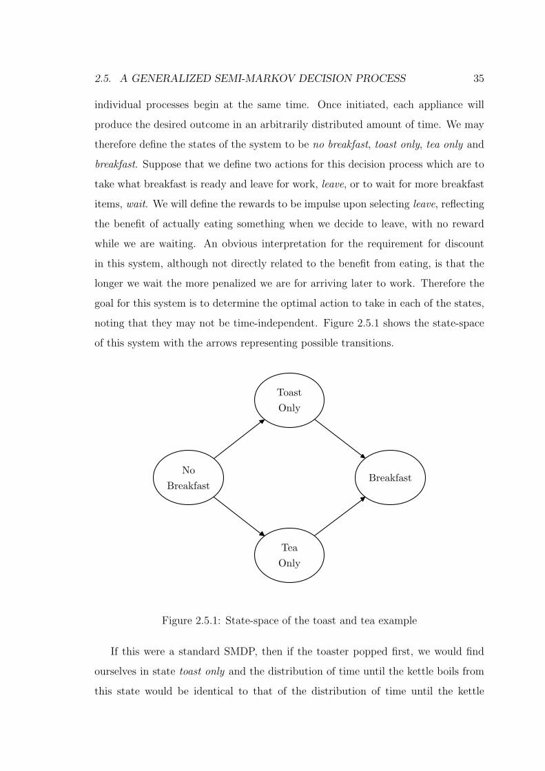
2.5. A GENERALIZED SEMI-MARKOV DECISION PROCESS 35
individual processes begin at the same time. Once initiated, each appliance will
produce the desired outcome in an arbitrarily distributed amount of time. We may
therefore define the states of the system to be no breakfast, toast only, tea only and
breakfast. Suppose that we define two actions for this decision process which are to
take what breakfast is ready and leave for work, leave, or to wait for more breakfast
items, wait. We will define the rewards to be impulse upon selecting leave, reflecting
the benefit of actually eating something when we decide to leave, with no reward
while we are waiting. An obvious interpretation for the requirement for discount
in this system, although not directly related to the benefit from eating, is that the
longer we wait the more penalized we are for arriving later to work. Therefore the
goal for this system is to determine the optimal action to take in each of the states,
noting that they may not be time-independent. Figure 2.5.1 shows the state-space
of this system with the arrows representing possible transitions.
No
Breakfast
Toast
Only
Tea
Only
Breakfast
Figure 2.5.1: State-space of the toast and tea example
If this were a standard SMDP, then if the toaster popped first, we would find
ourselves in state toast only and the distribution of time until the kettle boils from
this state would be identical to that of the distribution of time until the kettle
36 CHAPTER 2. MARKOV PROCESSES
boils from state no breakfast. That is, due to the Markovian nature of the state-
space in an SMDP, we are essentially modelling the scenario that when the toaster
pops, we throw out the water in the kettle and start it again. While an SMDP is
very versatile, this is clearly not how our process should behave. The fact that a
GSMDP can model asynchronous events and that our action selection of wait, if it
is selected, does not disable any active events means that the kettle can continue
boiling as though the toaster never popped.
Note that in our breakfast example, the model requires from the outset two event
clocks, one for each appliance as from the no breakfast state; we have two appliances
competing to be the first to produce an item of the breakfast. At this point, we
propose a slight change in framework that will aid in the modelling of the process
we will be considering throughout this thesis. Referring back to Figure 2.5.1, a
transition from no breakfast to toast only occurs following the distribution of time
it takes for the toaster to pop if it is the first event to trigger in this system. We
can however define the holding time distribution of the no breakfast state as the
minimum of the two event distributions. Therefore, we can split this holding time
distribution probabilistically, based on the likelihood of one event occurring before
the other, to define the distribution of time until transitioning to either of the single
event states.
This subtle change of reference has meant that in our example, we no longer
require to keep track of two event clocks, and can define all state transition distri-
butions in terms of a single global time-clock. The net result is a transformation
of our GSMDP into a time-inhomogeneous SMDP. We mentioned in the previous
section that it may not be feasible to analyze such decision processes. Nevertheless,
we will use this transformation throughout this thesis as it simplifies the analysis,
and also because available techniques for GSMDPs are even more scarce than those
for inhomogeneous SMDPs.

Chapter 3
Phase-Type Distributions
3.1 Introduction
Phase-type (PH ) distributions have been used in a variety of stochastic modelling
applications since their introduction by Neuts [65] in 1975. Examples of the diverse
areas in which PH distributions have been employed are: Fazekas, Imre and Telek
[30] use PH distributions in their model of broadband cellular networks; Marshall
and McClean [61] utilize a form of PH distributions to model the duration of stay
for the elderly in hospital; and Aalen [1] investigates the use of PH distribution in a
range of survival analysis problems, including the modification of an existing AIDS
incubation model which preserves the original essential properties. The formulation
of PH distributions allows the Markov structure of stochastic models to be retained
when they are used in place of the familiar exponential distribution. They, however,
allow for much greater flexibility and, as will be seen, have the ability to replace non-
exponential distributions while supplying computational tractability to the model.
With his “method of stages” in 1917, Erlang [28] was the first person to extend
the exponential distribution. Here, a nonnegative random variable is defined as the
time taken to move through a fixed number of stages, spending an exponentially
distributed amount of time with a fixed positive rate in each. This distribution is
now simply referred to as the Erlang Distribution.
This first extension paved the way for other distributions utilizing the familiar
37

38 CHAPTER 3. PHASE-TYPE DISTRIBUTIONS
exponential distribution. The hyper-exponential distribution is where an exponen-
tially distributed random variable is selected probabilistically from a set of expo-
nential distributions with differing parameters. The Coxian distribution, described
here as in [6], is similar to that of the Erlang distribution, but in this situation,
after each of the exponentially distributed sojourn times in a particular stage, there
is a possibility of jumping straight to the end rather than continuing through all
of the remaining stages. Figure 3.1.1 illustrates the aforementioned distributions
graphically as Markov chains where the nonnegative random variable defined for
each is the time taken to reach state 0. Note that 0 < qi ≤ 1 for i = 1, . . . , (p− 1),
0 < αi < 1 for i = 1, . . . , p with∑p
i=1 αi = 1 and λi > 0 for i = 1 . . . p. In each
of these generalizations however, it is worth noting that from a stage/state point of
view, once a state is left it is never again revisited. PH distributions with this prop-
erty are referred to as acyclic, due, clearly, to the lack of cycles in the underlying
state-space.
3.2 Phase-Type Representations
Neuts [65] went further in his generalization of a “method of stages” whereby he de-
fines a phase-type random variable as the time taken to progress through the states
of a finite-state evanescent Markov chain until absorption. PH distributions are
hence a very versatile class of distributions in that they have a simple probabilistic
interpretation. The use of PH distributions often leads to algorithmically tractable
solutions due to their Markovian nature. Quantities of interest such as the distri-
bution and density functions of PH distributions can be expressed in terms of the
initial phase distribution α and the infinitesimal generator of the defining Markov
chain, T .
Consider a continuous-time Markov chain with finite phase (state) space S =
{0, 1, 2, . . . , p} where phase 0 is absorbing. Let the initial phase probability distri-
bution be (α0,α), where α = (α1, α2, . . . , αp) and∑p
i=0 αi = 1, and the infinitesimal
generator of this Markov chain be Q. The random variable X corresponding to the

3.2. PHASE-TYPE REPRESENTATIONS 39
2) The p-phase generalized Erlang distribution
3) The hyper-exponential distribution
1
2
p
0
λ1
λ2
λp
α1
α2
αp
1 2 3 p 0λ1 λ2 λp
1 2 3 p 0q1λ1 q2λ2 λp
4) The p-phase Coxian distribution
(1− q1)λ1 (1− q2)λ2
λ1 0
1) The exponential distribution
Figure 3.1.1: Graphical representation of the exponential, generalized Erlang, hyper-
exponential and Coxian distributions

40 CHAPTER 3. PHASE-TYPE DISTRIBUTIONS
time to absorption of this chain is said to have a continuous phase-type distribution.
The infinitesimal generator may be written in block matrix form as
Q =
0 0
t T
.
Here, 0 is a 1× p vector of zeros and follows from the absorbing nature of phase 0.
The column vector t = (t1, t2, . . . , tp)′ represents the absorption rate from phase i
for i = 1, 2, . . . , p. T = [Tij] is a p× p matrix where, for i, j = 1, 2, . . . , p,
Tij ≥ 0 for i 6= j,
and
Tii < 0 with Tii = −ti −p∑
j=1j 6=i
Tij.
The PH distribution is said to have a representation (α,T ) of order p. The matrix
T is referred to as the PH -generator of the distribution and, as it explicitly defines
t, there is no need for t to appear in the representation. Similarly the the point mass
at zero, α0, is not necessary in the representation as it is completely determined by
α.
A PH distribution with such a representation has distribution and density func-
tions given by
F (x) =
α0, x = 0
1−αexp(Tx)e, x > 0,
and
f(x) = −αexp(Tx)Te, x > 0,
respectively [66], where e is a p× 1 vector of ones.
Returning to the examples given in Figure 3.1.1 we may now write down their
respective representations:
1. The exponential distribution has a representation
α = (1)
T = (−λ) .

3.2. PHASE-TYPE REPRESENTATIONS 41
2. The p-phase generalized Erlang distribution has a representation
α = (1 0 . . . 0)
T =
−λ1 λ1 0 . . . 0
0 −λ2 λ2 . . . 0
0 0 −λ3. . . 0
......
. . . . . ....
0 0 0 . . . −λp
.
3. The hyper-exponential distribution has a representation
α = (α1 α2 . . . αp)
T =
−λ1 0 . . . 0
0 −λ2. . . 0
.... . . . . .
...
0 0 . . . −λp
where αi > 0 for i = 1, . . . , p and∑p
i=1 αi = 1.
4. The p-phase Coxian distributions have representations of the form
α = (1 0 . . . 0)
T =
−λ1 q1λ1 0 . . . 0
0 −λ2 q2λ2 . . . 0
0 0 −λ. . . 0
......
. . . . . ....
0 0 0 . . . −λp
where 0 < qi ≤ 1 for i = 1, . . . , (p− 1).

42 CHAPTER 3. PHASE-TYPE DISTRIBUTIONS
3.3 Using Phase-Type Distributions
A very useful property of PH distributions is that they are dense in the set of all
distributions on [0,∞) [81]. However, the usefulness of this property, as mentioned
by Neuts [66], can be limited. Some distributions are simply not PH -type; for
example, those distributions that do not have rational Laplace-Stieltjes transforms
[81]. Even those distributions that are PH -type may have representations that
require many phases. From a modelling perspective, a large number of phases may
be prohibitive with regard to the use of PH distributions.
Nevertheless, for the purpose of modelling it may not be necessary to use an
exact representation. PH approximations of general distributions can be used to
reflect the essential qualitative features of the distribution. When using a PH ap-
proximation in place of a general distribution within a model, often the model gains
some amount of computational tractability. Therefore, through the interpretation
of numerical results, the approximation provides much useful information about the
behaviour of the model. In approximating a probability distribution with a PH
distribution, the parameters α and T need to be selected such that the “distance”
between the approximated distribution and the approximating PH distribution is
minimized in some sense. The most common distance metrics used to date are
those of maximum likelihood, moment matching and least squares. Descriptions of
these methods can be found in most elementary texts on mathematical statistics
such as Wackerly, Mendenhall and Scheaffer [90]. There are algorithms available
for matching qualitative features of a general distribution and particular forms of
PH distributions such as those presented in Bobbio and Telek [14] and Asmussen,
Nerman and Olsson [5].
Issues of uniqueness and minimal order arise for any given PH distribution. As
noted in Neuts [66], a PH distribution may have many distinct irreducible rep-
resentations, not all of which are of minimal order. Consider the following PH
distribution which is adapted from an example in Botta, Harris and Marchal [15].

3.3. USING PHASE-TYPE DISTRIBUTIONS 43
The PH (hyper-exponential) distribution with density
f(x) =2
32e−2x +
1
35e−5x
has representations (α,T ), (β,U ) and (κ,V ) given by
α =(
23
13
)
T =
−2 0
0 −5
,
β =(
25
35
)
U =
−2 2
0 −5
,
and
κ =(
0 12
12
)
V =
−3 1 1
1 −4 2
1 0 −6
.
This demonstrates the concept of the possibility of representations of higher than
minimal order and also non-uniqueness. The non-trivial questions of determination
of minimal order and non-uniqueness of representations for PH -type distributions
have been considered in many publications, such as [22], [23], [38] and [69]. These
issues, particularly non-uniqueness, have ramifications when fitting distributions to
empirical data, or other distributions, and are particularly relevant in the context
of PH distributions. Consider that the general representation of a PH distribution,
(α,T ), of order p requires p2 + p parameters. Due to a property of the Laplace-
Stieltjes transform of a general PH distribution, we find that a PH distribution can
in fact be parameterized with only 2p parameters. This over-parameterization leads
directly to a possibility of non-uniqueness via the redundant parameters. When fit-
ting however, the problem of over-parameterization can be bypassed by restricting
the approximation to that of a Coxian distribution which requires only 2p parame-
ters. Osogami and Harchol-Balter [70] provide some conditions for matching the first
3 moments of a general distribution with that of a Coxian distribution. As discussed
in Faddy [29], however, even Coxian distributions can have multiple representations,

44 CHAPTER 3. PHASE-TYPE DISTRIBUTIONS
so while over-parameterization has been addressed, the issue of non-uniqueness has
not. The overall problem of non-uniqueness is not well understood and, in general,
the effect that a change of parameters, including redundant parameters, will have on
the shape of a PH distribution is not known a priori. Also, for a given representation
it is not possible, in general, to determine a minimal order representation.
From a modelling perspective, however, the issues of minimal order and non-
uniqueness in many ways become secondary to closeness of approximation when
substituting for general distributions. Lower order approximations may be preferable
from a computational perspective, but a necessity of minimal order is unlikely.
When using PH distributions for modelling, the phases can be thought of in two
different ways. Firstly, the phases can represent physical characteristics and, in
these instances, the model determines the structure of the PH representation to
be used. Secondly, the phases can be purely fictitious, in which case the class of
PH distributions provides a versatile, dense and algorithmically tractable class of
distributions defined on the non-negative real numbers. Nevertheless, due to non-
uniqueness, one should be cautious in assigning a physical interpretation to the
phases of the PH approximation in such circumstances.

Chapter 4
The Race
4.1 Introduction
In this chapter and throughout this thesis we will be considering continuous-time
decision processes where the time spent in each state may follow an arbitrary dis-
tribution. In particular, we are interested in non-exponential distributions. We will
be predominantly focusing on distributions that have an exact phase-type repre-
sentation, or may be approximated arbitrarily closely by phase-type distributions.
Recall the property from Section 3.3 which states that phase-type distributions are
dense in the field of non-negative distributions. We employ such distributions, as
we will use some of the phase properties in order to gain insight into possible so-
lution techniques. When using the phase-type representation, we maintain analytic
tractability and some Markovian properties [66] that will aid in the solution of the
decision processes.
The specific problems of interest are those where we have independent distri-
butions in competition with one another, a process that we refer to as the race.
Imagine a scenario where we have a set of particles that we release toward a desti-
nation and then record their individual arrival times at that destination. One area
of interest, here, is that at any time after the release of the particles we will have a
subset of the particles present at the destination and at any point we may ask the
question whether or not it is worth waiting for any more of the particles to arrive.
45

46 CHAPTER 4. THE RACE
This decision will of course depend on the value we place on having certain particles
present and possibly how long they have been at the destination.
If time is of no interest and we make the reasonable assumption that the reward
received is increasing in the number of particles present, then the obvious decision
would be to wait until all particles are present and then take the required action in
order to receive the reward. In reality, however, we can rarely ignore time in such
a way. As an example, consider an online telephony server waiting to merge audio
packets from multiple sources before forwarding the combined packet to a single
destination as in McMahon et al. [63]. In this situation, merging too early results in
lost/delayed individual packets and hence reduces the quality of service rating of the
audio transmitted from those sources that are omitted. Waiting for all sources to
arrive, however, delays all audio streams, reducing the quality of service for all audio
streams at once. Therefore, we may ask the question of when the server should stop
waiting and merge those that have already arrived.
The race can also occur in areas other than telecommunications traffic. If we are
waiting for money from multiple sources to invest in a single venture, then delaying
the investment leaves less time to gain revenue before some fixed date when the
gain (or loss) is realized. There is even a foreseeable agricultural application of
the process, whereby multiple crops may be planted at the same time but, due to
soil, weather and possibly other conditions, the crops may yield at different times.
Assuming, due to restrictions on harvesting such as setup costs and timing, that all
crops must be harvested at the same time, then we must choose when to actually
harvest via some reward function for early and late harvesting.
In the next section the race that we will be considering throughout this chap-
ter is formally described. Following that, in Section 4.3, we consider the decision
process formed by the race when the information provided to the decision maker
is limited. In Section 4.4, we first consider a more general decision process when
the decision maker has full knowledge of the system. Then, the race is formulated
in this framework and an example of the race is given, demonstrating two different
solution techniques.

4.2. THE RACE – FORMAL DESCRIPTION 47
4.2 The Race – Formal Description
Consider a system with K, K ≥ 1, independent identically distributed holding
times. That is, we are considering a race involving K particles heading toward a
destination, each following an independent but identical arrival distribution. Let the
distribution function of the arrival time for each particle be denoted P (t). When
the global clock starts running and the system is initiated at time 0, we allow a
particle to be in one of two scenarios. Either it begins its journey from its source
and arrives at the destination following the specified arrival time distribution, or,
for completeness, it may already be present at the destination. For those particles
that do not begin at the destination, we define the conditional probability that it
arrives in an interval (a, b], given that it had not arrived up until, and including, a,
as
Pc(a, b) =
∫ b
a
dP (τ)
1−∫ a
0
dP (τ)
. (4.2.1)
Once a particle is present at the destination, it remains there. Also, all particles
are guaranteed to arrive at the destination eventually (arrive with probability 1).
It is possible to relax these two constraints in such a way that particles can expire
if they spend too much time at the destination or get lost on their way to the
destination. Nevertheless, for the purposes of this investigation, these relaxations
simply add extra complexity to the system. By maintaining these constraints we give
our process an obvious guaranteed termination state when all particles are present
and prevent cycles in the state-space. Both are properties that we will exploit in
order to solve the problem, as shall be seen later.
At any time, s ≥ 0, the system can be in any of K + 1 states, which are the
natural states representing the number of expired distributions and hence arrived
particles at time s. We include in the state-space an artificial termination state
which is absorbing and will be referred to as state −1. As such, our complete state-
space is I = {−1, 0, 1, . . . , K}. For notational convenience we define the natural
states of the system as I ′ = {0, 1, . . . , K}. Once the termination state is entered

48 CHAPTER 4. THE RACE
via a decision made at a decision epoch, the process of waiting for more particles is
terminated. We assume that there is no reward gained whilst the process is running
and the only reward that can be received is upon deciding to terminate the process.
Once this is done, no further reward may be gained. The reward received upon
termination is based on those particles that are present at the destination when
termination occurs.
Suppose that the reward structure for this race is such that each particle present
at the destination when termination is selected contributes 1 unit of reward. If
termination is selected at some future time x then we must calculate the net present
value at time s of the termination reward using a discount factor
D(s, x) = e−∫ x
sβ(τ)dτ ,
where we allow for a time-dependent discount rate β(t). We nevertheless restrict
the permissible choices of β(t) such that
d
dxD(s, x) ≤ 0 (4.2.2)
and
D(s, x)→ 0 as (x− s)→∞ for all s ≥ 0, x ≥ s. (4.2.3)
The condition in inequality (4.2.2) enforces the idea that the net present value of
a state at some time in the future is not greater than its current value. Condition
(4.2.3) dictates that, as the difference between the current and termination times
becomes large, the net present value drops to zero.
While occupying state i there are K − i concurrent distributions, all in compe-
tition with another to cause a transition to the next natural state of the system.
In the context of these concurrent distributions, each with their own time clock, we
have essentially described the race as a generalized semi-Markov decision process
(GSMDP), see Section 2.5. This is due to the fact that when a particle’s distri-
bution expires; that is, the particle arrives at the destination causing a change in
state, the remaining outstanding particles’ arrival distributions do not reset. Rather,
the remaining concurrent distributions continue as though the transition had not
occurred, and it is this property that classes the system as a GSMDP.

4.3. RESTRICTED VISION 49
4.3 Restricted Vision
An important feature of any decision process is the definition of the policy class
under consideration. One aspect is the information available to the policy, which
can be thought of as the vision of the decision maker. The vision of the decision
maker directly relates to decision epochs in terms of their frequency and availability.
In this section, we consider the race when the decision maker has restricted vision
of the process. For the various classes of restricted vision policies, policy evaluation
equations are developed and how optimal policies may be found is described.
4.3.1 Blind
When the decision maker is classed as a blind observer, we have a situation where
the decision maker must try and make a decision with only limited information
available. Here, the observer still has knowledge of all the system dynamics such
as arrival distributions of particles and reward structure. The restriction in an
information sense is the ability of the observer to see arrivals of particles at the
destination as they happen and hence knowledge of the actual state of the system.
Such a scenario may arise when polling a system for state information is quite costly
in some sense. Therefore, once the state is known, it may be desirable to construct
a policy from that point without the need for more state information. We may even
have a system where only a single observation of state is possible and no further
observations are available to the decision maker. To allow a non-trivial starting
point for the decision maker, we will study scenarios where the decision maker is
supplied with knowledge of the state of the system at a particular time and must
make a decision based only on that information, combined with knowledge of the
system dynamics.
Let us define 2 actions for the race, a default action a0 = continue and another
action a1 = terminate. When the default action a0 is selected, the underlying process
of arrivals continues unhindered and no reward can be received. Selecting action a1
forces an immediate transition to the artificial termination state, which is otherwise
50 CHAPTER 4. THE RACE
not reachable, and the decision maker receives the available reward. In terms of
vision there is only one decision epoch when the state of the system is supplied to
the decision maker, say at s, as no further state transitions are visible. As such,
the selection of action a0 at any time s is rather uninteresting as, without another
available decision epoch, the process will never be terminated and no reward will
be received. If a1 is selected at s then, as termination is instantaneous, the process
is ended and reward is received immediately. These two options, however, while
straightforward, make no use of the information the decision maker has regarding
the underlying dynamics of the system. To do so, we expand the class of acceptable
policies for the race such that the decision maker may delay termination until some
future time, denoted xi(s) where xi(s) ≥ s for all states i ∈ I ′ and possible decision
epochs s ≥ 0. These termination times xi(s) define the decision whereby at decision
epoch s, if the system is known to be in state i, then the default continue action
is selected and then the process is terminated at xi(s). In allowing these decisions
to be made, the decision maker now has the option of delaying termination, thus
enabling the possibility of delaying actually receiving reward, in the hope that the
reward received will be greater than that available at s. It is nevertheless important
to note that the termination time is not another decision epoch, but simply some
future time at which the decision maker has specified for terminating the process.
Utilizing knowledge of the dynamics of the system, when the decision maker is
supplied with information such that the system is in state i at time s and follows a
policy that terminates the process at xi(s), we may write down the expected present
value of the decision process under a given policy as
Vi(s, xi(s)) =[
i + (K − i)Pc(s, xi(s))]
D(s, xi(s)), ∀i ∈ I ′ , ∀s ≥ 0. (4.3.1)
The term in square brackets of equation (4.3.1) represents the expected number of
particles present at the destination at the chosen time of termination and hence, as
all particles contribute 1 unit of reward, also the reward received at termination. As
the state is i at time s, there will definitely still be i particles present at termination.
The remaining (K− i) particles are each weighted by the conditional probability, as
defined in equation (4.2.1), that an arrival occurs in the interval (s, xi(s)] given that
4.3. RESTRICTED VISION 51
it had not occurred by time s. Finally, as this is the reward received at termination,
we multiply by the discount factor applied over the appropriate interval to give the
expected value of the process at the decision epoch s.
In terms of optimality, we seek to find a policy, being a complete set of termi-
nation times, x∗i (s) such that Vi(s, x
∗i (s)) ≥ Vi(s, xi(s)) for all i ∈ I ′, s ≥ 0 and
x∗i (s) ≥ s. We define the optimal value and optimal termination time in state i at
time s as
V ∗i (s) = sup
xi(s)
Vi(s, xi(s)) (4.3.2)
and
x∗i (s) = argsup
xi(s)
Vi(s, xi(s)) (4.3.3)
respectively.
As the decision maker cannot see transitions as they occur, the value equations
for each state are independent of one another. Therefore, solving equations (4.3.2)
and (4.3.3) involves finding the maximum value, and its location, of a 1-dimensional
function.
For an example of optimal policy selection, consider a race between 3 identical
particles each with an arrival time following an Erlang order 2 distribution with rate
parameter λ = 3. Here we set β(t) = 1 for all t, such that we have simple constant
exponential decay of the value functions.
If the system is occupying state 3 at decision epoch s, then with the described
system parameters we find that optimality gives x∗3(s) = s for all s ≥ 0. This
policy is intuitively obvious as, once all 3 particles are present, there is no reason
to delay the action of termination. If the system is occupying state 2 at decision
epoch s, however, we find that the optimal decision regarding when to terminate,
x∗2(s), depends on the value of s. Consider the optimal waiting time from time
s before termination, that is x∗2(s) − s. Figure 4.3.1 shows a plot of the optimal
waiting time for any decision epoch s ∈ [0, 2]. From Figure 4.3.1, for 0 ≤ s ≤ 23,
the optimal waiting time from s is 0, giving an optimal policy of x∗2(s) = s. For
decision epochs in the range [0, 23] we find that waiting a reasonable time for the

52 CHAPTER 4. THE RACE
arrival of the last particle, as we cannot see the arrival itself, costs more in terms
of discounting than the benefit gained from its possible arrival and so we choose
immediate termination. When s > 23, however, we find that the optimal waiting
time becomes strictly positive. This means the optimal policy of termination has
x∗2(s) > s, with (x∗
2(s) − s) < ∞. In other words, we wait from s until x∗2(s)
and then terminate the process to receive the maximum possible expected value of
reward. For this range of decision epochs, we know that the final arrival has not
occurred by s and, due to the properties of non-memoryless conditional probability
distributions, it becomes more likely that this final arrival will occur close to the
current decision epoch. In this instance, a small wait becomes beneficial in that we
allow more time for the arrival to occur without discounting the expected reward
too much. Therefore, we have found a time-dependent optimal policy that specifies
immediate termination when s ≤ 23
and a finite wait before termination when s > 23.
0 0.2 0.4 0.6 0.8 1 1.2 1.4 1.6 1.8 20
0.01
0.02
0.03
0.04
0.05
0.06
0.07
0.08
0.09
0.1Optimal Waiting Time in State 2 with 3 Particles
s
x 2* (s)
− s
Figure 4.3.1: Optimal waiting time in state 2 given decision epoch at time s
It is important to note that the actual waiting time x∗i (s) − s is finite for all
systems with a blind observer, regardless of the initial state i. An infinite wait
would result in no reward received, as the process would never be terminated due

4.3. RESTRICTED VISION 53
to the lack of future decision epochs.
4.3.2 Partially Observable
While the field of Markov decision processes has received much attention, that of
partially observable Markov decision process has received comparably much less.
A partially observable Markov decision process (POMDP) is a generalization of a
Markov decision process that permits uncertainty regarding the state of a Markov
process [64]. The decision maker must therefore approximate the current state when
information about state is limited, in order to decide on a course of action to be
taken. In our context, the notion of partial observability on the part of the decision
maker is the same as that of a POMDP, but we make no restriction on remaining
in the realm of straightforward Markov decision processes. In fact, we will see later
that our problem actually falls into the class of time inhomogeneous semi-Markov
decision processes and, as such, we can draw no results from the existing literature
for our specific problem.
In the previous section, we studied a situation where the decision maker is given
a snap-shot of the system at a particular time and no further information. We now
expand the information available to the decision maker by also allowing the system
to notify the decision maker when certain states of interest are reached. This is an
important class of policies where the naivety of the blind observer does not suffice,
but it is not possible to see every state transition as it happens. Many situations
exist where the assumption of complete state information at all times is invalid.
An example may involve a decision to be made based on the state of a machine
that is comprised of various internal and unobservable components. Sensors used to
measure the state may give noise-corrupted readings and these readings themselves,
effectively being exact state observations, may be costly. This type of problem
appears regularly in the artificial intelligence literature, see for example Simmons
and Koenig [82] and Parr and Russell [71], where regular state information via
measurement updates can be quite costly and yet decisions must continue to be
made regardless.

54 CHAPTER 4. THE RACE
Consider, as in McMahon et al. [63], the problem of aligning and merging audio
packets in a data network environment. Here, we choose to delay some packets
that have already arrived in order to hopefully perform a merge later on with more
packets included. In this problem, sequential packets from the same source arrive
approximately every 10ms and therefore a new race is formed every 10ms. For even
a moderate number of sources in this fast moving environment it can become too
computationally intensive to know at all times how many packets have arrived, and
hence, in terms of the race, which state is occupied.
Here we investigate the possible improvements that can be made with regard to
optimal policies and expected values when more information is made available to the
decision maker. Rather than simply supplying snap-shots of the system, in essence
making a sequence of blind decisions, suppose we can supply the decision maker
with the knowledge that certain states have been entered. In particular, suppose
the decision maker now has the ability to see when the last particle has arrived,
that is, when the process reaches the all arrived state. This availability of state
information when all particles have arrived is in fact implemented in the system
studied in [63].
Although it is possible to allow vision of any subset of the states, we choose
at this point just to focus on the aforementioned state. Allowing vision of states
other than all arrived leads to value equations that can become quite difficult to
solve analytically, an aspect that will be explored in more detail when we study the
policies when the decision maker has full knowledge of the system at all times. The
all arrived state of the race is, however, a special case in that it leads to no other
natural state. This means that there is no need to wait for any further arrivals and,
as such, the maximum expected value and the associated optimal policy is trivially
determined. We can exploit this property to write down a set of value equations
that are still essentially independent from one another, as in the blind case, and are
therefore easy to solve to determine the optimal policy.
In the previous section, we stated the expected present value of the decision pro-
cess at a given decision epoch in equations (4.3.1). These equations were formulated

4.3. RESTRICTED VISION 55
from the perspective of the expected number of arrivals present at the destination
at the time of termination. An equivalent set of value equations can be written in
terms of the probability of being in each state at termination as
Vi(s, x) =
[
K−i∑
j=0
(i + j)
(
K − i
j
)
Pc(s, x)j(1− Pc(s, x))(K−i)−j
]
D(s, x)
for all i ∈ I ′ and s ≥ 0, where we have let xi(s) = x to simplify the notation.
Consider in isolation the all arrived term from the above set of value equations,
KPc(s, x)(K−i)D(s, x).
Here we have the reward of all K particles weighted by the probability that the
outstanding K − i particles, given a starting state of i, have arrived in the interval
(s, x], all multiplied by the discount factor to bring the value received at termination,
x, back to the present, s. This term behaves in a blind fashion in that it does not
know if state K is actually reached before the specified horizon of termination.
The allowable policies for the partially sighted observer are the same as those
for the blind observer, with the addition of the specification that, as soon as all
arrivals have occurred, the decision maker is notified and another decision epoch
occurs. Let θ be the first hitting time on state K, where s < θ ≤ x. The decision
maker is informed at the hitting time θ and is supplied with a new decision epoch
at θ. The decision maker therefore has 2 possible decision epochs under this class
of policies. The first is the initial decision epoch at s when system information is
supplied, where, as in the case of the blind observer, there is the option of immediate
or delayed termination. Then, at the random hitting time θ of state K another
decision epoch is made available to the decision maker. Intuitively, as there are no
further arrivals to wait for, the best decision at this epoch must be to terminate
immediately. In state K, if we are to terminate the process at y ∈ [θ,∞) then the
present value at epoch θ is given by VK(θ, y) = KD(θ, y). Due to the properties
of the discount factor, VK(θ, y) is clearly a maximum when y = θ, confirming our
intuition. Therefore, with a view toward optimal behaviour, we force the decision
maker in this class of polices to terminate the process immediately upon hitting

56 CHAPTER 4. THE RACE
state K at decision epoch θ, that is let y = θ. To incorporate this random decision
epoch we must integrate the reward VK(θ, θ) = K against the probability density
that state K is entered at θ, for θ ranging from s up until state i’s chosen termination
time x. The resultant all arrived term is thus given by∫ x
s
K (K − i)Pc(s, θ)K−i−1D(s, θ) dPc(s, θ), for i ∈ I ′\{K}
and obviously K for i = K.
The expected present value of the decision process under the given partially
sighted policy can therefore be expressed for all s ≥ 0 and x ≥ s as
Vi(s, x) =
[
K−i−1∑
j=0
(i + j)
(
K − i
j
)
Pc(s, x)j(1− Pc(s, x))(K−i)−j
]
D(s, x)
+
∫ x
s
K (K − i)Pc(s, θ)K−i−1D(s, θ) dPc(s, θ), for i ∈ I ′\{K}, (4.3.4)
with the value of state K being VK(θ, θ) = K, as defined by the policy class.
Again, in terms of optimality, we seek to find a policy x∗i (s), such that Vi(s, x
∗i (s))
≥ Vi(s, xi(s)) for all i ∈ I ′\{K}, s ≥ 0 and x∗i (s) ≥ 0 as in equations (4.3.2) and
(4.3.3). Note that the value equations (4.3.4), as in the blind policy, are independent
of one another. Therefore, these equations, although slightly more complicated than
their blind counterparts, may be solved for the optimal value and hence policy via
maximization of a 1-dimensional function. Returning to the example used in the
previous section of 3 sources each with an Erlang order 2 arrival distribution, we may
compare the optimal policies and values of the partially sighted and blind policies.
Considering state 2, being the simplest non-trivial state, we see that we also
find a time-dependent optimal policy as in the blind scenario. For initial decision
epoch s ≤ 512
, the optimal value from equation (4.3.4) is 2, with optimal policy
x∗2(s) = s. This means that at any decision epoch, s, before time 5
12, if we are
occupying state 2 then the optimal policy dictates that we terminate the process
immediately and receive a reward of 2. When s > 512
, we actually find that x∗2(s) =
argsupx2(s) V2(s, x2(s)) = ∞, which has the physical interpretation of waiting until
the next decision epoch. That is to say, if we are in state 2 after time 512
, then the
best policy is to just wait until the third particle arrives, which itself is a decision

4.3. RESTRICTED VISION 57
epoch, and then terminate the process. This is an added feature to the possible
optimal policies when compared to the blind scenario, as we now have a later state
that is visible to the decision maker and hence have available an extra decision
epoch.
Figure 4.3.2 shows the optimal expected value functions in state 2 for both the
blind and sighted policies for a range of decision epochs. For decision epoch s with
0 ≤ s ≤ 23
the blind scenario has an optimal policy of immediate termination, giving
an optimal value of 2. For s > 23, the optimal policy involves a short wait before
termination as no further decision epochs are available to this policy class. Due to the
length of the wait, being of the order of 100ths of time units, the optimal expected
present value does not increase much beyond that of immediate termination. The
partially sighted scenario too has a time-dependent policy, where 0 ≤ s ≤ 512
gives
an optimal policy of immediate termination. For s > 512
, we see that V ∗2 (s) > 2 and
the optimal policy is such that termination is selected to be at infinity, effectively
resulting in a decision to wait until the third and final particle arrives.
0 0.2 0.4 0.6 0.8 1 1.2 1.4 1.6 1.8 21.75
1.8
1.85
1.9
1.95
2
2.05
2.1
2.15
2.2
2.25Optimal Expected Value in State 2 with 3 Particles
s
V2* (s
)
BlindPartial
Figure 4.3.2: Optimal expected value for state 2 at decision epoch s
The difference in the optimal values between the two policy classes for the same

58 CHAPTER 4. THE RACE
state emphasizes the advantage of having extra information available to the decision
maker, particularly when the all arrived state of the race is reached. The blind
decision maker has only the option of a finite wait at the initial decision epoch to
improve on the available reward at s. In comparison, the partially sighted decision
maker also has the added option of waiting until the last arrival occurs, gaining an
extra decision epoch and therefore better performance.
Figures 4.3.3 and 4.3.4 show the optimal expected value functions for states 1
and 0 respectively. For both, the optimal policy for the blind observer is a finite
wait, now of the order of 10ths of time units, before termination. The partially
sighted observer’s optimal policy is such that the waiting time is infinite, resulting
in the best policy being to always wait until the all arrived state is entered before
termination.
0 0.2 0.4 0.6 0.8 1 1.2 1.4 1.6 1.8 20
0.2
0.4
0.6
0.8
1
1.2
1.4
1.6
1.8
2Optimal Expected Value in State 1 with 3 Particles
s
V1* (s
)
BlindPartial
Figure 4.3.3: Optimal expected value for state 1 at decision epoch s
The partially sighted observer in states 1 and 0 follows a time-independent opti-
mal policy of waiting for all outstanding arrivals to occur without being able to see
any of the intermittent arrivals. A logical next step in the context of this example,
and the general race, is to investigate if the decision maker would behave differently

4.4. FULL VISION 59
0 0.2 0.4 0.6 0.8 1 1.2 1.4 1.6 1.8 20
0.2
0.4
0.6
0.8
1
1.2
1.4
1.6
1.8
2Optimal Expected Value in State 0 with 3 Particles
s
V0* (s
)
BlindPartial
Figure 4.3.4: Optimal expected value for state 0 at decision epoch s
if these intermittent arrivals were visible and to see the effect of this new policy class
on the optimal expected values attainable.
4.4 Full Vision
In the context of general decision processes, and for comparison with other solution
techniques, we now consider the situation when the decision maker has full knowl-
edge of the system and hence sees state transitions as they occur. Each time the
system changes state represents a decision epoch and at each decision epoch, the
decision maker chooses when to terminate the process, which may be immediately,
not at all or anywhere in between. When a new decision epoch is encountered, the
decision made at the last decision epoch becomes redundant, as more information
is known about the system and a new decision is made, based on this information.
There is a small but growing amount of literature on the theory of partially ob-
servable Markov decision processes, as mentioned earlier. However, the standard
assumption in the published literature, for the most part, is that the decision maker

60 CHAPTER 4. THE RACE
is able to see all transitions as they occur. Markov decision processes, semi-Markov
decision processes and both finite and infinite horizon dynamic programming prob-
lems all rely on this assumption that the class of allowable policies has knowledge of
the state of the system at all times [12], [74], [43]. In this section, the value equations
from Chapter 6 of Janssen and Manca [49], which apply to much more complicated
processes than the race, are described. We then modify their value equations to
incorporate decision policies. Finally, the race is formulated in this framework and
we give examples of possible solution techniques.
4.4.1 Value Equations
We begin by describing the value equations for a reward process, as these will form
the building blocks for policy evaluation in the corresponding decision processes. In
particular, value equations for semi-Markov reward processes (SMRPs) are analyzed
extensively by Howard [43]. These are processes where the transitions from state to
state may follow an arbitrary distribution. Various forms of reward may be collected,
or lost, along the way, depending on the time spent in each state and the actual
transitions, from some starting time, s say, until some designated time horizon, t say.
Given a set of transition probabilities and a reward structure, the expected value
of the process starting in each state may be calculated over the interval of interest.
Although Howard [43] covers a wide range of topics with regard to SMRPs, he
remains in the realm of time-homogeneity. Later, we will require evaluation of non-
homogeneous semi-Markov reward processes and so we adopt notation similar to
that in Janssen and Manca [49], which contains the generality needed.
Consider a system with state-space S = {0, 1, 2, . . . , N}. Then let us define, as in
[49], Jn ∈ S, n ∈ N, which represents the state at the nth transition and Tn ∈ R+,
n ∈ N, which represents the time of the nth transition. We can then define the
kernel of the process, P = [Pij(s, θ)], i, j ∈ S, where
Pij(s, θ) = P[Jn+1 = j, Tn+1 ≤ θ | Jn = i, Tn = s].
This defines the probability that the next transition is to state j at or before time

4.4. FULL VISION 61
θ, conditional on the fact that the system occupied state i at time s, for all θ ≥ s.
We now describe the general reward structure as defined in Chapter 6 of [49].
Each state may provide a permanence reward, ϕi(u), which is reward gained for
remaining in state i and in the general setting it is permitted to be a function of the
absolute time, u ≥ 0, for all i ∈ S. There are impulse rewards, γij(u), received for a
transition from state i to state j and again these may be a function of the absolute
time of the transition. A continuous-time discount factor is defined in [49] with
a time-dependent discount rate in the same manner as we defined D(s, x) earlier,
without enforcing our added restrictions (4.2.2) and (4.2.3). Thus, calculations of
the present value of the process looking into the future may be performed whilst
allowing time-varying discount rates β(t).
The value of the process, meaning the total reward paid or received, from time
s until the time horizon at t, discounted back to time s, is therefore defined, as in
[49], as
Vi(s; t) =
(
1−∑
k∈S
Pik(s, t)
)
∫ t
s
ϕi(α)D(s, α)dα
+∑
k∈S
∫ t
s
[(∫ θ
s
ϕi(α)D(s, α)dα
)
(4.4.1)
+(
γik(θ) + Vk(θ; t))
D(s, θ)
]
dPik(s, θ), ∀i ∈ S, ∀s ∈ [0, t].
The first term in equation (4.4.1) represents the value of the permanence reward
for remaining in state i when no transitions from state i (including transitions to
itself) occur in the interval [s, t]. The second term evaluates the reward that may
be accrued when a transition occurs at time θ ∈ [s, t]. These are all probabilistically
weighted via the density of the transition kernel at θ over the likelihood of each of
the possible next states. Specifically, we include the value of the permanence reward
for remaining in state i up until time θ and the impulse reward for a transition to
state k at θ, plus the value received given the process starts in state k at time θ
over the remaining duration until the horizon t. Finding the analytic solution of this
system of equations is, in general, the same as finding the solution of (effectively)
a system of Volterra equations of the second kind, which is by no means a simple

62 CHAPTER 4. THE RACE
task.
4.4.2 Policy Evaluation
Now that we have defined value equations for our reward process, we may include
the effect of actions, and hence policies. Supposing that actions can determine tran-
sition probabilities and reward received, finding the overall effect of these decisions
becomes an integral part of determining the optimal actions to take at all decision
epochs to receive the best possible expected reward. Semi-Markov decision processes
are given substantial treatment in Howard [43]; however, the problems referred to
are strictly time-homogeneous. It is also mentioned that the solution techniques
described are for discrete-time SMDPs only. As such, in the following section we
continue to use notation similar to that in Janssen and Manca [49] and implement
the necessary changes to accommodate the introduction of policies into that more
general framework.
Here we define for each state i ∈ S a set of possible actions Ai which may be
selected when the process is in state i. For each action a ∈ Ai we introduce a
transition kernel which we call Pa where Pa = [P aij(s, θ)] and P a
ij(s, θ) = P[Jn+1 =
j, Tn+1 ≤ θ | Jn = i, Tn = s, action a ∈ Ai selected at s ]. This defines the
probability that, being in state i at time s, the next transition is to state j at or
before time θ given action a is selected at time s.
The expected present value of a particular state now depends on the action
selected in that state at that decision epoch and the actions selected in all subsequent
states, where, each time a transition occurs, the decision maker gains a new decision
epoch. Let Πt be the set of all possible policies that the decision maker may follow
for the described process with a fixed time horizon t. A policy πt ∈ Πt completely
defines the decisions to be made in all states i ∈ S at all times from 0 until the
specified horizon t. These decisions, as in our specific examples earlier, include the
possibilities of delayed actions in the class of policies under consideration. Define
a default action a0 ∈ Ai for all i ∈ S such that when a0 is selected the underlying
process continues under action a0, which we think of as being unaffected by the

4.4. FULL VISION 63
decision maker. Decisions, being elements of a policy πt, are functions such that
[πt]i(·) : R+ →
{
(Ai, R+ ∪ {∞})
}
, ∀i ∈ S. (4.4.2)
That is, for a given state i ∈ S and decision epoch s, a decision defines an action,
a ∈ Ai, and time of action, xi(s) ∈ [s, t]. This delay involves the selection of the
default action a0 until xi(s), at which point action a is selected only if no state
transitions occur, and hence no new decision epochs were encountered, between s
and xi(s).
At a new decision epoch, all previous decisions are replaced by their current and
therefore newer counterparts. Note that, due to the potentially time-inhomogeneous
nature of the process, a decision [πt]i(s) may or may not prescribe the same action
and delay as [πt]i(s′) for s 6= s′, or similarly if the horizon t were to change.
We also note at this point that, in general, decisions could potentially involve the
specification of far more complex courses of action. For example, we could define our
allowable class of policies to be such that an optimal decision could specify a delayed
action, a1, followed by a further delayed action a2, and so forth, if no transitions
occur in the relevant time intervals of interest. While this added complexity may
be useful for accurate representation of an actual process, we feel that allowing such
policies at this level of investigation is an unnecessary complication. Such extensions
of the class of allowable policies could be implemented on a model by model basis if
desired. Henceforth, in this chapter we will restrict our allowable policies to those
that specify decisions as defined in equation (4.4.2).
Now that actions may be delayed arbitrarily, we define a decision based proba-
bility transition kernel P(a,xi(s)) = [P(a,xi(s))ij (s, θ)]. Here, P
(a,xi(s))ij (s, θ) is the proba-
bility that, being in state i at time s, the next transition is to state j at or before
time θ when decision [πt]i(s) = (a, xi(s)) is selected at s.
We now describe the decision extension of equation (4.4.1) which defines the
present value of the process when decisions are selected following a particular policy
πt ∈ Πt. The expected present value in state i at decision epoch s following policy

64 CHAPTER 4. THE RACE
πt is given by
V πt
i (s; t) =
(
1−∑
k∈S
P[πt]i(s)ik (s, t)
)
∫ t
s
ϕi(α)D(s, α)dα
+∑
k∈S
∫ t
s
[(∫ θ
s
ϕi(α)D(s, α)dα
)
(4.4.3)
+(
γik(θ) + V πt
k (θ; t))
D(s, θ)
]
dP[πt]i(s)ik (s, θ), ∀i ∈ S, ∀s ∈ [0, t].
When policy πt is applied to the system, the probability transition functions in
state i at decision epoch s under the decision [πt]i(s) = (a, xi(s)) are given, for all
i, j ∈ S, a ∈ Ai and s ∈ [0, t], xi(s) ∈ [s, t], by
P(a,xi(s))i,j (s, θ) =
P a0i,j (s, θ), if θ < xi(s),
P a0i,j (s, xi(s)) +
(
1−∑
k∈S
P a0i,k(s, xi(s))
)
P ai,j(s, θ)
1− P ai,j(s, xi(s))
,
if θ ≥ xi(s).
Now we wish to find the policy, or policies, that maximize the value functions
as described above. In general, simply evaluating a fixed policy can be a non-trivial
task and yet we wish to search through all possible policies to find one that gives
the maximum present expected value at time s. That is, we are endeavouring to
find a solution to the problem of finding π∗t such that V
π∗t
i (s; t) ≥ V πt
i (s; t) for all
πt ∈ Πt, i ∈ S and s ∈ [0, t] for the given time horizon t.
4.4.3 The Race Revisited
Equation (4.4.3) demonstrates the available complexity of decision processes that
may be studied in this manner. At this point, however, we return to a specific sim-
plified example, namely the race as described in Section 4.2, of the general decision
process described above, in order to provide a few canonical examples which we will
explore in detail.
The reward structure for the race under consideration will therefore involve no
permanence rewards and the impulse rewards will be constant with respect to time

4.4. FULL VISION 65
and defined as
γi,j =
i, i ∈ I ′, j = −1,
0, otherwise.
We also assume a constant discount rate β, β > 0, such that the discount factor is
D(s, t) = e−β(t−s). We enable the possibility of termination by defining the actions
that may be taken in each state. Here we allow two actions, the same for all
states, being to continue the process, allowing natural transitions with regard to
the expiration of holding time distributions, or to terminate the process, forcing a
transition to the absorbing termination state. In the notation used earlier, Ai = A =
{a0, a1} for all i ∈ I ′ where a0 = continue and a1 = terminate. When action a0 is
selected, states of the process change via the expiration of holding time distributions
and, as the termination state cannot be reached in this manner, no reward is received.
Reward can only be received by selecting action a1 and moving to the absorbing
termination state. Once there, the process can never return to the natural states
and so we may consider the process to have ended. As reward can be received once
and only once, the problem becomes one of finding when to terminate the process
in order to maximize this once-off reward. This in turn leads to a definition of the
allowable decision rules as those which, at decision epoch s, choose action a0 until
time xi(s) ∈ [s, t ], and then choose action a1 at xi(s), for all i ∈ I ′. Note here that
we need only refer to the time at which we terminate, as this is the only action
that may be delayed, other than our default continue action. As such, we drop the
specific reference to action a1 in our decision notation earlier and a decision is now
simply the time at which we choose the only non-default action available, terminate.
We may therefore essentially think of an eligible policy πt as a vector-valued function
πt ={
(x0(s), x1(s), . . . , xK(s)), s ∈ [0, t]}
, (4.4.4)
specifying the times that the terminate action should be chosen in each state at
decision epoch s.
The policy in equation (4.4.4) is written with explicit dependence on the interval
over which the policy is being applied, to enable the idea that a policy may specify
66 CHAPTER 4. THE RACE
a termination time that is based on the time horizon t and not just on the decision
epoch s. In all cases, we do no worse in terms of the maximum value possible in
state i by letting t → ∞, in essence allowing an infinite horizon and admitting
more knowledge of the system. Thus, the value when using an optimal policy over
a finite horizon, t say, is such that Vπ∗
t
i (s; t) ≤ Vπ∗
∞i (s;∞) for all i ∈ I ′. As we are
after the policy that maximizes our value functions, it serves no purpose, from a
mathematical viewpoint, to limit the system to one with a finite horizon. We will
therefore be considering only the infinite horizon scenario from this point forward.
For notational simplicity, we choose to leave out the horizon at∞, where it is clear.
For example, as we no longer restrict the decision to terminate to be made before
some finite horizon, we can re-write (4.4.4) as
π ={
(x0(s), x1(s), . . . , xK(s)), s ∈ [0,∞)}
, (4.4.5)
leaving in the time dependence where appropriate.
Although each holding time distribution has its own expiration clock, we may
think of the time until the next expiration in terms of a single global clock. A tran-
sition from state k to k + 1 is caused by the first of the concurrent active holding
times expiring. The distribution of this expiration is therefore equivalent to the dis-
tribution of the minimum of the active conditional holding times. The distribution
of time between any state transitions is always the minimum distribution of some
number of active conditional holding times, which can be expressed in terms of a
single clock. We no longer need to keep explicit track of each individual expiration
clock and as such we have formulated our GSMDP, which has multiple concurrent
clocks, into a time-inhomogeneous SMDP where our decision maker requires only
knowledge of a single global clock, in this case absolute time.
Given the sequential nature of the state-space, the value equations as given in
equation (4.4.3) for a given policy π ∈ Π hence reduce to
V π−1(s) = 0, (4.4.6)
V πK (s) =
∫ ∞
s
Ke−β(θ−s)dPxK(s)K,−1 (s, θ), (4.4.7)

4.5. THE RACE – EXPONENTIAL SYSTEM 67
V πi (s) =
∫ ∞
s
V πi+1(θ)e
−β(θ−s)dPxi(s)i,i+1 (s, θ)
+
∫ ∞
s
ie−β(θ−s)dPxi(s)i,−1 (s, θ), for i ∈ I ′\{K}, (4.4.8)
where
Pxi(s)i,i+1 (s, θ) =
Pi,i+1(s, θ), if θ < xi(s),
Pi,i+1(s, xi(s)), if θ ≥ xi(s),for i ∈ I ′\{K},
Pxi(s)i,−1 (s, θ) =
0, if θ < xi(s),
1− Pi,i+1(s, xi(s)), if θ ≥ xi(s),for i ∈ I ′\{K},
PxK(s)K,−1 (s, θ) =
0, if θ < xK(s),
1, if θ ≥ xK(s),
and
Pxi(s)i,j (s, θ) = 0 for all other i, j ∈ I.
The problem now becomes one of finding the termination times xi(s), for all i ∈ I ′,
which maximizes these value equations.
Due to the directional and sequential nature of the natural states in the state-
space, along with a known end state being when all particles have arrived at the
destination, we find an obvious method of solution. We may solve this particular
problem using backward recursion, in a similar manner to the technique often used
in finite-horizon dynamic programming [12] albeit in a slightly different context.
Here, we may easily find the optimal solution, both in the sense of value and policy,
for state K. Then we may use this solution in order to find an optimal solution for
state K − 1 and so forth. We now give a small example of this solution technique
before moving to more complicated realizations of the race.
4.5 The Race – Exponential System
Note that complexity of the optimal solutions may increase as we move further away
from the end state. Depending on the arrival time distributions for the race we are
68 CHAPTER 4. THE RACE
considering, we may find that the iterative solution technique described previously
becomes prohibitive, which will be demonstrated in Chapter 5. Before complicating
matters, however, we show the usefulness of these value equations with a simple
exponential version of the race. Consider a situation where each of the holding time
distributions is in fact exponentially distributed. Therefore, with exponential arrival
distributions and exponential discount we have effectively described a memoryless
race. We begin by solving the value equations for this system and then, as this
memoryless version can be described as Markov decision process, we utilize a solution
technique for Bellman’s optimality equations [12] in this Markovian environment.
4.5.1 Value Equations
Suppose that each of the holding time distributions is exponentially distributed with
parameter λ. It is a well known and easily provable property that the distribution of
the minimum of n exponential distributions is itself an exponential distribution, with
a parameter equal to the sum of the individual competing exponential distributions’
parameters. Therefore, we have the probability of a transition from state i to state
i + 1 in the interval [s, θ ] given by
Pi,i+1(s, θ) = 1− e−(K−i)λ(θ−s).
At this point, we define wi(s) to be the waiting time in state i at time s when
applying the policy π(s), with w∗i (s) being the obvious optimal analogue. The wait-
ing time is given by wi(s) = xi(s) − s for all i ∈ I ′ and s ≥ 0 and may take
values in the range [0,∞]. Mapping the possibilities to physical characteristics, fi-
nite non-zero values of wi(s) specify that continue is selected at s with the process
then terminated at the appropriate time. When wi(s) = 0 the policy determines
immediate termination, while wi(s) =∞ indicates that termination should in effect
never be selected and the policy is to just continue the process; that is, select the
continue action, until another arrival and hence decision epoch occurs. These last
two scenarios, terminate immediately and continue (indefinitely), form the corner-
stone of the decision process when the decision maker has full vision and hence sees

4.5. THE RACE – EXPONENTIAL SYSTEM 69
all transitions, or equivalently, decision epochs.
The integral value equations (4.4.6)–(4.4.8) are not as complicated as in the
general distribution case and, due to the sequential nature of their relationship, we
may solve for the optimal decision and hence value at each stage in succession. For
the example described in this section, equation (4.4.7) becomes
V πK (s) = Ke−β(xK(s)−s),
which has a clear maximum of K when (xK(s) − s) = 0 as we would expect. Via
this value equation, we find that the obvious optimal policy in state K is to always
terminate immediately. As such, w∗K(s) = w∗
K = 0 with V π∗
K (s) = K ≡ V π∗
K for all
s ≥ 0 and thus we no longer require the functional dependence on time.
The next state of interest is K − 1 and from equations (4.4.8) we find that
V πK−1(s) =
(
λK
λ + β
)
+
(
(K − 1)−(
λK
λ + β
))
e−(λ+β)(xK−1(s)−s) .
It can be shown via a simple derivative test that the maximum of this function
occurs either when wK−1(s) = xK−1(s)− s = 0 or infinity. Therefore we deduce the
optimal waiting time in state K − 1
w∗K−1 =
0, if K − 1 ≥ λK
λ + β,
∞, otherwise,
with optimal expected value
V π∗
K−1 = max
{
λK
λ + β, K − 1
}
,
where the first element in the maximum corresponds to continue and the second
to terminate. Once again, the optimal waiting time and value is independent of
s resulting in a time-homogeneous optimal policy and so the dependence on s has
been dropped.
We can continue in this fashion for all states down to and including state 0. The
solution to the entire problem, being an optimal policy specifying optimal actions
70 CHAPTER 4. THE RACE
in every state, is given by
w∗K = 0,
w∗i =
0, if i ≥ (K − i)λV π∗
i+1
(K − i)λ + β,
∞, otherwise,
for i ∈ I ′\K (4.5.1)
where
V π∗
K = K,
V π∗
i = max
{
(K − i)λV π∗
i+1
(K − i)λ + β, i
}
for i ∈ I ′\K, (4.5.2)
where again the first element in the maximum corresponds to continue and the
second to terminate. The equality in equation (4.5.1) is largely an arbitrary choice.
In the case when the two terms are equal, any choice of termination time results
in an equivalent optimal expected present value. Here, we decide that we will
terminate the process as soon as the decision to continue performs no better. As we
are comparing a fixed value with a random variable, we deem it preferable to take
the immediate reward. This means that we are opting to take a guaranteed reward,
which is the standard mentality in the decision process literature.
Due to the memoryless property of the exponential distribution, we see that the
optimal decision rule for each state, and hence overall optimal policy, is constant for
all time. The optimal policy itself only depends on the exponential rate parameter,
λ, the discount rate, β, and of course the state itself. Hence, all reference to the
current time s has been omitted from equation (4.5.1) and we say that the solution
to the decision process is time-homogeneous.
4.5.2 MDP Approach
We could, however, have approached this problem from a different viewpoint. The
time taken to transition between the natural states of the system is exponentially
distributed as described earlier. The natural states of the system therefore form a
Markov chain with state transition rates as shown in Figure 4.5.1.

4.5. THE RACE – EXPONENTIAL SYSTEM 71
0Kλ
1(K − 1)λ
2 K − 22λ
K − 1λ
K
Figure 4.5.1: Markov chain state-space of the exponential system
We can now construct an infinitesimal generator, Q0, incorporating all of the
states in I, which describes the transitions of a continuous-time Markov chain when
we do not interfere with the process, that is, under the action continue, a0. For the
exponential example under consideration,
Q0 =
0 0 0 0 · · · 0 0 0
0 −Kλ Kλ 0 · · · 0 0 0
0 0 −(K−1)λ (K−1)λ · · · 0 0 0...
.... . . . . . . . . . . .
......
0 0 0 0 · · · −2λ 2λ 0
0 0 0 0 · · · 0 −λ λ
0 0 0 0 · · · 0 0 0
,
where we have ordered the states {−1, 0, 1, 2, . . . , K − 2, K − 1, K} as in I.
We can also construct an infinitesimal generator, Q1, for the transition to the
termination state -1 when we select the action terminate, a1. The rate that we
choose for the transition to the termination state, α say, needs to be the same for all
states and arbitrarily large, as we are in effect modelling an instantaneous transition
to the termination state. Therefore
Q1 =
0 0 0 · · · 0 0
α −α 0 · · · 0 0
α 0 −α · · · 0 0...
.... . . . . . . . .
...
α 0 0 · · · −α 0
α 0 0 · · · 0 −α
,
using the same state ordering as for Q0.

72 CHAPTER 4. THE RACE
With these two transition rate matrices, one for each of the possible actions, the
constant discount rate β and the reward structure, we have essentially defined a
(time-homogeneous) continuous-time Markov decision process.
Recall the Bellman-Howard optimality equations from Section 2.3.3 for discrete-
time MDPs, which we rewrite here as
V ∗i = max
a∈A
{
γai + δ
∑
j∈I
P aij V ∗
j
}
, (4.5.3)
where γai is the reward received in state i when action a is chosen, δ is the discount
factor over an interval, I is the state-space and P aij is the probability of moving from
state i to j during a discrete time interval when action a is selected.
Via the technique of uniformization [52], our continuous-time MDP may be trans-
formed into a discrete-time MDP [74]. Let c represent our uniformization parameter
which we choose such that c ≥ maxi∈I, m=0,1
{− [Qm]ii}. By uniformizing the transition
rate matrices, the discrete-time probabilities of state transitions are given by
Pam
= I +1
cQm for m = 0, 1.
In order to maintain the idea of an instantaneous transition to the termination state,
we must choose c = α which fits within the requirements of the uniformization
parameter as α is arbitrarily large. This results in a column of 1s as the first column
of Pa1
meaning that when terminate is selected, the system is guaranteed to be in
the termination state at the next decision epoch.
The reward structure in this notation is
γam
i =
0, m = 0,
i, m = 1, i 6= −1,
0, m = 1, i = −1,
being no immediate reward if we select action a0, continue, and the reward for all
particles present, and hence the state of the system, if we select action a1, except for
the termination state in which we can receive no reward. The discrete time discount
factor for the uniformized system is δ = cc+β
, which is the expected discount over
4.5. THE RACE – EXPONENTIAL SYSTEM 73
the exponentially distributed length interval with mean 1c
when a constant discount
factor β is applied.
Although we argued earlier that α needed to be arbitrarily large, we find that in
the uniformization process it suffices that α ≥ maxi∈I{−[Q0]ii}. Therefore, for the
purpose of this example, we choose the uniformization parameter c to be c = α = Kλ
which satisfies the enforcement of our immediate termination criterion and allows
for convenient arithmetic. We may now solve equations (4.5.3) using many methods,
including value iteration and policy iteration of Bellman’s optimality equation [12].
Again, due to the directional nature of the state-space, we may start at the all
arrived state and work backwards in a dynamic programming approach. In this
state, with V ∗−1 = 0, we find
V ∗K = max
{
Kλ
Kλ + βV ∗
K , K
}
= max
{
0, K
}
= K,
where the first element in the maximum corresponds to continue and the second to
terminate.
In state K − 1, Bellman’s optimality equations yield the recursive expression
V ∗K−1 = max
{
Kλ
Kλ + β
(
(K − 1)λ
KλV ∗
K−1 +λ
KλV ∗
K
)
, K − 1
}
,
which has solution
V ∗K−1 = max
{
λK
λ + β, K − 1
}
.
We can continue in such a manner for all of the remaining states, and we find that
the optimal solution using Bellman’s optimality equations is identical to equations
(4.5.2),
V ∗K = K,
V ∗i = max
{
(K − i)λV ∗i+1
(K − i)λ + β, i
}
for i ∈ I ′\K

74 CHAPTER 4. THE RACE
where the optimal policy is implied by which of the two arguments of the max
operator is larger, where the first element in the maximum corresponds to continue
and the second to terminate.
The integral value equations in Section 4.4.2, which can be difficult to solve,
provide the same solution to the discretized Markov Decision Process and, therefore,
we have provided an alternative solution technique for continuous time MDPs for
exponential versions of the race. The advantage of the integral value equations is
that they can handle non-exponential distributions, although, on the other hand,
realistically they require a known state where the optimal decision is obvious in
order to solve them even moderately efficiently. Bellman’s optimality equations
can handle Markov processes much more complicated than the race, but rely on
time-homogeneity for ease of solution.
In the next chapter, we study the properties of optimal policies when the arrival
time distributions are Erlang, a non-memoryless and hence time-dependent distri-
bution, and investigate the suitability of both of these solution techniques, along
with some others that we develop.

Chapter 5
The Race – Erlang System
5.1 Introduction
We now consider the scenario of the race, in the context of full vision, where the ar-
rival times of particles at the destination follow an Erlang distribution. The reasons
we choose the Erlang distribution at this stage of investigation are two-fold. Firstly,
the Erlang distribution is not memoryless, in that the conditional arrival probability
distribution for a particle, as defined in equation (4.2.1),
Pc(a, b) =
∫ b
a
dP (τ)
1−∫ a
0
dP (τ)
,
depends on the absolute value of a and not just the length of the interval (b − a).
Therefore we may be forced to consider policies that depend on the absolute time
of the process, as opposed to those in a strictly Markovian environment such as the
exponential race as discussed in Section 4.5. Secondly, the Erlang distribution has
two well known representations for its density and distribution functions. Under the
interpretation that the Erlang distribution is a special case of the gamma distribution
where the shape parameter is integer, an Erlang order p distribution with rate
parameter λ > 0 has density and distribution functions
f(x) =λpxp−1e−λx
(p− 1)!,
75

76 CHAPTER 5. THE RACE – ERLANG SYSTEM
and
F (x) = 1−(
e−λx
p−1∑
j=0
(λx)j
j!
)
,
respectively, for x ≥ 0, where p ≥ 1 and integer.
The polynomial that appears in the distribution function will appear frequently
throughout this chapter. In order to simplify notation to some extent, we define the
polynomial of degree r− 1, ξ(r,α)(x), where r ≥ 1 and α are specified parameters, to
be
ξ(r,α)(x) =r−1∑
j=0
(αx)j
j!∀x ∈ R, (5.1.1)
which is, in fact, a truncation of the exponential series, eαx =∑∞
j=0(αx)j
j!, containing
r terms.
There also exists an exact PH representation of an Erlang order p distribution
with density and distribution functions given by
f(x) = −αexp(Tx)Te, x > 0,
and
F (x) =
α0, x = 0,
1−αexp(Tx)e, x > 0,
where α is a 1× p vector given by
α = (1 0 . . . 0) ,
T is a p× p matrix given by
T =
−λ λ 0 . . . 0
0 −λ λ . . . 0
0 0 −λ. . . 0
......
. . . . . ....
0 0 0 . . . −λ
,
and e is a p× 1 vector of ones.

5.2. VALUE EQUATIONS 77
Throughout this chapter and the next, we will make the assumption that p > 1
and integer. The Erlang distribution with p = 1 is in fact the exponential distribu-
tion, and the exponential race has been considered, and solved, in Section 4.5.
In Section 5.2 we will attempt to solve this decision process using the value
equations defined earlier in Section 4.4.2. We will use the non-PH representation of
the Erlang distribution therein for two main reasons. Using this form of the Erlang
distribution allows for easier algebraic manipulation and hence demonstration of
properties, when compared to requiring an analytic expression from the exponential
of a matrix. Secondly, most distributions in the literature are defined by their
density/distribution functions in non-PH form. As such, we consider this to be the
natural starting point for our investigation.
At the beginning of Section 4.1, we stated that we will be predominantly focusing
on distributions that have an exact phase-type representation, or those that may be
approximated arbitrarily closely by phase-type distributions. The Erlang distribu-
tion does have an exact PH representation, and this form is utilized in Chapter 6
where a new technique exploiting the underlying phases of the distribution is con-
structed. The solutions found in this chapter therefore provide a benchmark against
which to compare the methods developed in Chapter 6.
5.2 Value Equations
We now begin to solve the value equations (4.4.6)–(4.4.8) for the optimal policy,
where each of our particles arrive at the destination following an Erlang distribution.
As the state-space of the system is the number of arrivals that have occurred, we
must first formulate the probability transition kernel for this system. Recall that
a transition from state i to i + 1 is caused by the first of the concurrent active
holding times expiring. The distribution of this expiration is therefore equivalent
to the distribution of the minimum of the active conditional holding times. As in
the exponential case, there exists a convenient representation for the minimum of
multiple Erlang distributions. Therefore, we have the probability of a transition

78 CHAPTER 5. THE RACE – ERLANG SYSTEM
from state i to state i + 1 in the interval [s, θ ] given by
Pi,i+1(s, θ) = 1−(
e−λθξ(p,λ)(θ)
e−λsξ(p,λ)(s)
)(K−i)
∀i ∈ I ′\{K}, (5.2.1)
using the polynomial defined in equation (5.1.1).
Throughout this chapter, we will continue to refer to both the waiting time in
a state and the absolute time of termination where appropriate. As in the previous
chapter, we denote wi(s) (w∗i (s)) to be the waiting time (optimal waiting time) in
state i at time s when applying the policy π (π∗). The waiting time in state i is
given by wi(s) = xi(s) − s, for all i ∈ I ′ and s ≥ 0, and it may take values in the
range [0,∞], where xi(s) is the absolute time of termination.
Note that in state −1, equation (4.4.6) gives the property that all policies result
in a value of 0. As we consider the process to be terminated in this state, no further
decisions need to be made and thus we will omit this state in our discussions of
optimal policies. We therefore begin our analysis of this system in state K, the all
arrived state.
5.2.1 State K
As has been the case with all race examples thus far, the intuitive optimal policy
in state K, when all particles have arrived, is trivial. We nevertheless include the
analysis here for completeness of solution. Equation (4.4.7) gives
V πK (s) =
∫ ∞
s
Ke−β(θ−s)dPxK(s)K,−1 (s, θ),
= Ke−βwK(s),
which has a clear maximum of K when wK(s) = 0, confirming our intuition. Via
this value equation, we find that the obvious optimal policy in state K is to always
terminate immediately. Therefore,
V π∗
K (s) = K, ∀s ≥ 0,
with optimal policy of w∗K(s) = 0 at every possible decision epoch s ≥ 0. Having
solved state K, we now make use of the recursive relationship between the states of
the system and focus on the next state of interest.

5.2. VALUE EQUATIONS 79
5.2.2 State K − 1
In state K − 1 we must decide how long to wait, for the last remaining particle
to arrive, before terminating the process. As there is only a single outstanding
particle, this problem is equivalent to that of the partially sighted observer as the
next state in the process must be the all arrived state. Thus, at decision epoch
s, say, the decision maker knows that there will be another decision epoch at the
hitting time, θ, of state K and must decide whether or not it is worth waiting until
θ. The optimality principle says that, when considering whether or not to wait, the
decision maker must behave optimally upon reaching state K in order to construct
an optimal policy for the system as a whole. Using the probability transition kernel
defined for this problem, the value equation (4.4.8) when i = K − 1 under a policy
that behaves optimally in state K gives
V πK−1(s) =
∫ ∞
s
V πK (θ)e−β(θ−s)dP
xK−1(s)K−1,K (s, θ) +
∫ ∞
s
(K − 1)e−β(θ−s)dPxK−1(s)K−1,−1 (s, θ),
= K
(
λ
λ + β
)p [(ξ(p,λ+β)(s)
ξ(p,λ)(s)
)
− e−(λ+β)wK−1(s)
(
ξ(p,λ+β)(xK−1(s))
ξ(p,λ)(s)
)]
+ (K − 1)e−(λ+β)wK−1(s)
(
ξ(p,λ)(xK−1(s))
ξ(p,λ)(s)
)
, (5.2.2)
for all s ≥ 0. The first integral in the first equality corresponds to the expected
present value if we hit level K before the termination time xK−1(s) determined by
the policy π. The second integral corresponds to the expected present value if the
termination time in state K−1 is reached before the final arrival occurs. The actual
value equation once the integration is performed loses most of its obvious physical
interpretation; however, this step is required in order to analyze various properties,
particularly its maximum value.
The determination of where the maximum of this value function will occur is far
less simple than in the exponential system. For a given decision epoch s, we must
determine w∗K−1(s) ∈ [0,∞] that maximizes V π
K−1(s). For a policy that determines
immediate termination in this state, that is wK−1(s) = 0, we find not surprisingly
that V πK−1(s) = K − 1 for all s ≥ 0.

80 CHAPTER 5. THE RACE – ERLANG SYSTEM
Let
h(x) =
(
ξ(p,λ+β)(x)
ξ(p,λ)(x)
)
for x ≥ 0. We note that this function is strictly increasing on the domain x ≥ 0
and that 1 ≤ h(x) <(
λ+β
λ
)p−1. When a policy specifies continue, meaning never
terminate the process and wait for the final arrival, V πK−1(s) = K
(
λλ+β
)p
h(s) in the
limit as wK−1(s) → ∞. We can thus conclude, as the value function is bounded,
that the maximum value may occur with a waiting time of 0 or ∞. To answer the
question of whether it is possible that the maximum value can occur for a finite
non-zero waiting time, we can gain insight, as in the exponential system, by looking
at the partial derivative of the value function, equation (5.2.2), with respect to the
termination time xK−1(s). We find that
∂V πK−1(s)
∂xK−1(s)=
e−(λ+β)wK−1(s)
ξ(p,λ)(s)
[
(λ− (K − 1)β)(λxK−1(s))
p−1
(p− 1)!
− (K − 1)βξ(p−1,λ)(xK−1(s))
]
. (5.2.3)
The term outside the square brackets,
e−(λ+β)wK−1(s)
ξ(p,λ)(s)→ 0 as wK−1(s)→∞,
and is positive for all decision epochs s ≥ 0 and feasible waiting times wK−1(s) ≥ 0.
For the exponential system, the derivative of the value function could only be 0 as
wK−1(s)→∞. In the Erlang system, we find that the derivative of equation (5.2.2)
approaches 0 in the same manner, but is also 0 if the term inside the square brackets
of equation (5.2.3) equals 0, that is, if
(λ− (K − 1)β)(λxK−1(s))
p−1
(p− 1)!− (K − 1)βξ(p−1,λ)(xK−1(s)) = 0.
Consider the polynomial
g(x) = (λ− (K − 1)β)(λx)p−1
(p− 1)!− (K − 1)βξ(p−1,λ)(x)
for x ≥ 0. If (λ − (K − 1)β) ≤ 0, then every coefficient of the polynomial g(x)
is negative. By using Descartes’ rule of signs, as there are no changes in sign of

5.2. VALUE EQUATIONS 81
the coefficients, there are no real positive zeros of g(x). This directly implies that
there are no zeros of equation (5.2.3), and hence no possibility of an optimal value,
corresponding to a finite waiting time. On the other hand, if (λ − (K − 1)β) > 0
then there is a single change in sign of the coefficients and, by Descartes’ rule again,
there can be at most one real positive zero of g(x). Furthermore, Gauss improved
Descartes’ original rule by proving that when there are fewer real (positive) roots
of a polynomial than there are changes in sign, the difference between the two is
even. As there is no non-negative integer less than one such that their difference is
a multiple of two, there is exactly one positive zero of g(x) for system parameters
such that (λ− (K − 1)β) > 0. In this case, let the unique zero of g(x) be c, so that
g(c) = 0. Now, as ξ(p−1,λ)(0) = 1, g(0) = −(K − 1)β < 0 and so the derivative in
equation (5.2.3) will be negative on [0, c). As there is a single positive zero of g(x),
it must be positive on (c,∞) and hence the derivative in equation (5.2.3) must be
positive on the same interval. In this situation, the zero of the derivative of equation
(5.2.2) must correspond to a minimum. Therefore, when searching for the location
of the maximum of equation (5.2.2), we need only check a waiting time of 0 and∞.
With
limwK−1(s)→∞
V πK−1(s) = K
(
λ
λ + β
)p(ξ(p,λ+β)(s)
ξ(p,λ)(s)
)
and V πK−1(s) = (K − 1) for a policy specifying wK−1(s) = 0, the optimal policy for
this state is given by
w∗K−1(s) =
0, if K − 1 ≥ K
(
λ
λ + β
)p(ξ(p,λ+β)(s)
ξ(p,λ)(s)
)
,
∞, otherwise.
(5.2.4)
Note here that, unlike the earlier exponential example, the optimal policy potentially
depends on the absolute time s of the decision epoch.
When w∗K−1(s) = 0 or ∞ for all possible decision epochs s, we refer to the
optimal policy as time-independent. That is, the optimal decision is the same at
every decision epoch when state K−1 is first occupied. We note that it is common in
the literature to refer to such a policy as stationary. The term stationary, however,
has many, often subtly, different meanings, depending on the context in which it
82 CHAPTER 5. THE RACE – ERLANG SYSTEM
is used. We feel that, in the interest of clarity, it is better for us to be explicit
about policy dependence on absolute time. Particularly when we begin to speak
of time-dependence, it will be clear as to our meaning, as opposed to the potential
ambiguity when using descriptions such as non-stationary. To determine whether a
system results in a time-independent optimal policy, we must consider the conditions
in equation (5.2.4) in more detail.
Consider the inequality
K − 1 ≥ supx≥0
{
K
(
λ
λ + β
)p
h(x)
}
.
Since supx≥0 h(x) =(
λ+β
λ
)p−1, this is equivalent to the inequality
K − 1 ≥ K
(
λ
λ + β
)
, (5.2.5)
and with a little algebraic manipulation, is in turn equivalent to
λ ≤ β(K − 1). (5.2.6)
Therefore, an arrival rate parameter satisfying inequality (5.2.6) gives the result that
(K − 1) ≥ K(
λλ+β
)p ( ξ(p,λ+β)(x)
ξ(p,λ)(x)
)
for all x ≥ 0, with equality in the limit as x→∞,
if and only if λ = β(K − 1). This directly implies that the optimal policy given in
equation (5.2.4) determines immediate termination at every possible decision epoch
s ≥ 0 and hence the optimal policy is time-independent.
Now consider the inequality
K − 1 < infx≥0
{
K
(
λ
λ + β
)p
h(x)
}
,
which, as infx≥0 h(x) = 1, is equivalent to
K − 1 < K
(
λ
λ + β
)p
. (5.2.7)
Algebraic manipulation, again, yields the following inequality with respect to the
arrival rate parameter,
λ >β(
K−1K
) 1p
(
1−(
K−1K
) 1p
) ,

5.2. VALUE EQUATIONS 83
which, after multiplying the numerator and the denominator by K(
1 +(
K−1K
)p−1
p
)
,
becomes
λ >β(K − 1) + βK(K−1
K)
1p
1−K(K−1K
)1p + K(K−1
K)
p−1p
. (5.2.8)
When inequality (5.2.8) is satisfied, we have that K(
λλ+β
)p ( ξ(p,λ+β)(x)
ξ(p,λ)(x)
)
> (K − 1)
for all x ≥ 0. Thus, in terms of the optimal policy when this inequality is satisfied,
equation (5.2.4) results in wK−1(s) =∞ for all s ≥ 0 and once again we have found
a time-independent policy.
Let
l1 = β(K − 1) (5.2.9)
and
l2 =β(K − 1) + βK(K−1
K)
1p
1−K(K−1K
)1p + K(K−1
K)
p−1p
. (5.2.10)
Now, l1 ≤ l2 with equality only when K = 1 or p = 1. The system when K = 1 is
however rather uninteresting and trivial. Inequality (5.2.8) tells us that the optimal
policy, regardless of the decision epoch s, is to wait for the next arrival for all λ > 0.
As λ > 0 by definition, this result coincides with the obvious notion that with
no particles present at the destination, in order to receive any positive reward we
must always wait until the next, and only, particle arrives. On the other hand,
p = 1 results in an exponential system which we have already studied in Section
4.5. For more interesting systems with K > 1 and p > 1, there exists a non-zero
length interval (l1, l2] for λ such that the optimal policy in this state depends on the
absolute time, s, of the decision epoch and hence is time-dependent.
Suppose that K > 1 and λ ∈ (l1, l2]. Consider the function
q(x) = (K − 1)−K
(
λ
λ + β
)p
h(x)
for x ≥ 0. Recall that h(x) is a strictly increasing function and so q(x) is a strictly
decreasing function.

84 CHAPTER 5. THE RACE – ERLANG SYSTEM
In the interval of interest, λ ≤ l2, and hence, from inequalities (5.2.8) and (5.2.7),
we deduce that
K − 1 ≥ K
(
λ
λ + β
)p
.
Therefore, at x = 0, since h(0) = 1,
q(0) = (K − 1)−K(
λλ+β
)p
≥ 0,
with equality only when λ = l2. Similarly, as λ > l1 in the interval under consider-
ation, inequalities (5.2.6) and (5.2.5) give
K − 1 < K
(
λ
λ + β
)
.
Since limx→∞ h(x) =(
λ+β
λ
)p−1, we have that
limx→∞
q(x) = (K − 1)−K(
λλ+β
)
< 0.
Therefore, as q(x) is strictly decreasing for x ≥ 0, there exists a unique t ≥ 0 such
that q(t) = 0 with q(x) > 0 for x ∈ [0, t) while q(x) < 0 for x ∈ (t,∞).
Relating this back to optimal decision making, t is the absolute time such that
the expected present value of the future reward when waiting for the next arrival,
K(
λλ+β
)p ( ξ(p,λ+β)(t)
ξ(p,λ)(t)
)
, is equal to the reward for immediate termination at t, K−1.
We thus refer to t as the threshold time and when the system parameters are such
that a positive threshold time exists, it can be found as the unique solution to
K − 1 = K
(
λ
λ + β
)p(ξ(p,λ+β)(t)
ξ(p,λ)(t)
)
. (5.2.11)
For any decision epoch s < t, by our study of the function q(x), we have that
immediate termination provides a greater reward than that which we would expect
to receive for waiting and so the optimal policy for decision epochs in this range
is such that wK−1(s) = 0. When s = t, by definition of our policy, as we do not
expect to do better by waiting, immediate termination is also selected. For decision
epochs s > t, properties of q(x) tell us that we expect to do better by continuing the
process and waiting for the arrival of the last particle, in comparison to immediate
termination, and so the optimal policy here is wK−1(s) =∞.

5.2. VALUE EQUATIONS 85
Therefore, a time-dependent policy is such that a threshold time, 0 ≤ t < ∞,
exists whereby decision epochs at or before the threshold time specify immediate
termination while decision epochs after the threshold time specify waiting until the
next arrival. Table 5.2.1 summarizes the optimal policies for all possible combina-
tions of system parameters.
Table 5.2.1: Summary of optimal policies
System Parameters Optimal Policy Type Optimal Policy Description
λ ∈ (0, l1]† Time-independent Select terminate at every decision
epoch s ≥ 0.
λ ∈ (l1, l2]† Time-dependent Threshold time 0 ≤ t <∞
exists. Select terminate if s ≤ t
and select continue if s > t.
λ ∈ (l2, ∞) † Time-independent Select continue at every decision
epoch s ≥ 0.
† l1 and l2 as defined in equations (5.2.9) and (5.2.10).
By using Table 5.2.1, we can deduce whether state K − 1 will have a threshold-
based optimal policy by simply observing the system parameters. To simplify the
framework, we wish to represent this policy by a single parameter. An obvious
candidate is the threshold time t; however, to utilize this parameter we must modify
our action selection at the threshold time t, albeit only slightly. When t = 0,
although strictly speaking a time-dependent optimal policy, there is only 1 decision
epoch s = 0 where the optimal decision is to terminate. The expected value for
continuing the process in this situation is equal to that received upon termination.
Termination is selected only because it is conventional in the literature to take the
guaranteed reward if we do not expect to do any better by continuing. Therefore,
we will break the convention in this single instance to define a time-independent
policy of selecting continue at all decision epochs if the input parameters result in a
threshold time of t = 0. On the other hand, a threshold at t = ∞ from a practical

86 CHAPTER 5. THE RACE – ERLANG SYSTEM
point of view specifies an optimal decision of terminate immediately at all decision
epochs s ≥ 0. Henceforth, rather than considering the 3 categories from Table 5.2.1
separately, we will incorporate the time-independent policies into those defined with
a threshold time t. In other words, in state K− 1, a threshold of t = 0 or∞ defines
time-independent optimal policies while any finite non-zero threshold, 0 < t < ∞,
defines a conventional threshold policy.
To summarize the results thus far, the optimal values in state K − 1 at decision
epoch s are therefore given by
V π∗
K−1(s) = max
{
K
(
λ
λ + β
)p(ξ(p,λ+β)(s)
ξ(p,λ)(s)
)
, K − 1
}
, (5.2.12)
where the first element corresponds to waiting for the next arrival, selecting the
continue action, and the second corresponds to immediate termination.
Let us now return to the common example of Sections 4.3.1 and 4.3.2 of a system
with K = 3 particles arriving according to an order p = 2 Erlang distribution with
arrival rate parameter λ = 3 and an overall system discount parameter of β = 1.
The results in Section 4.3.2 for this system are identical to those we will see here, as
a partially sighted decision maker in state K− 1 has the same information available
as that of a fully sighted decision maker. Nevertheless, here the solution will go into
more detail, illustrating the properties derived throughout this chapter thus far.
Equations (5.2.9) and (5.2.10) for this set of system parameters give l1 = 2 and
l2 = 2 +√
6 ≈ 4.4495. As λ ∈ (l1, l2], we know that the optimal policy will be
a threshold policy. To find the time at which the optimal decision changes, that
is the threshold time t, we must solve equation (5.2.11) with the current system
parameters. Equation (5.2.11) is therefore
2 = 3
(
3
4
)2(1 + 4t
1 + 3t
)
,
which has solution t = 512
.
Figure 5.2.1 shows the expected present values at decision epoch s when the
terminate and continue actions are selected. We see that before the threshold time
the maximum value attainable from these two possible decisions is to immediately
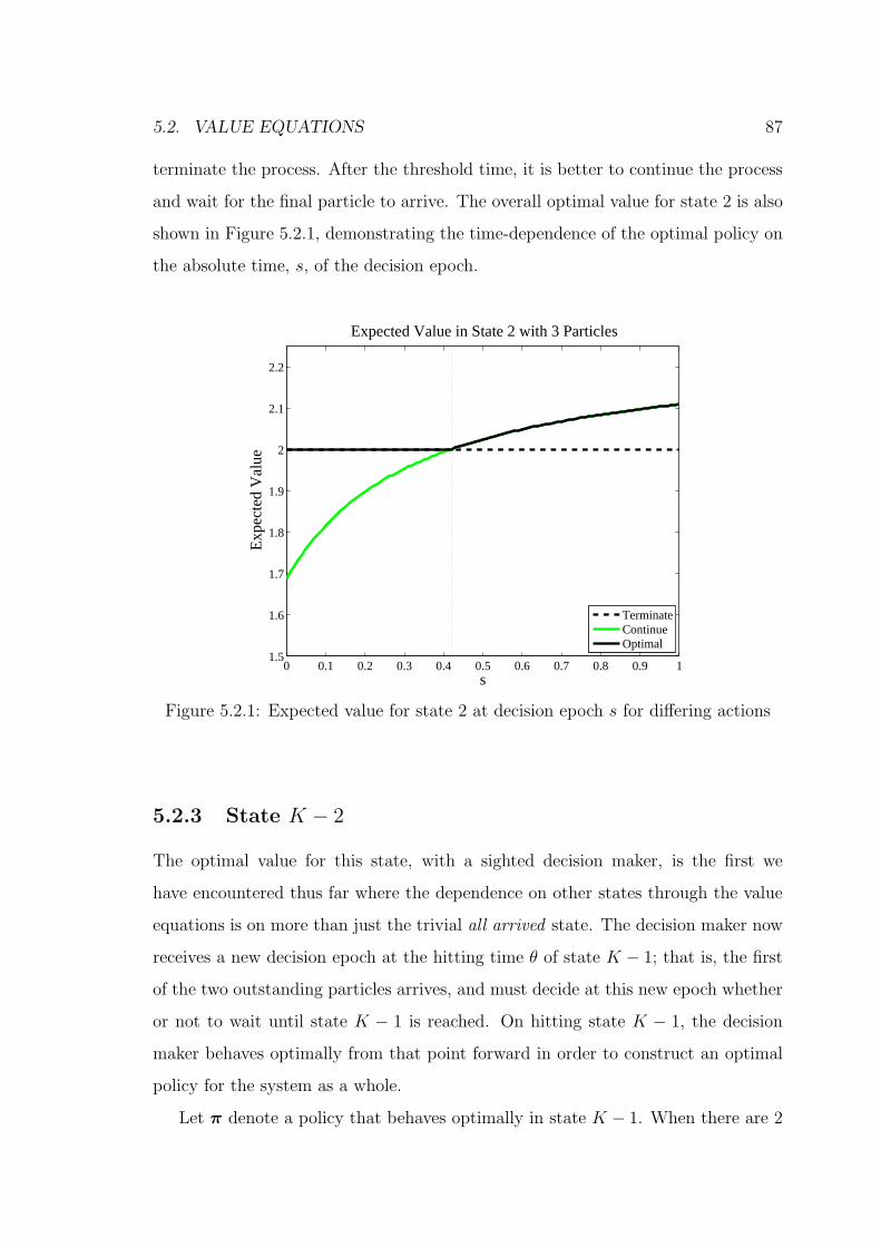
5.2. VALUE EQUATIONS 87
terminate the process. After the threshold time, it is better to continue the process
and wait for the final particle to arrive. The overall optimal value for state 2 is also
shown in Figure 5.2.1, demonstrating the time-dependence of the optimal policy on
the absolute time, s, of the decision epoch.
0 0.1 0.2 0.3 0.4 0.5 0.6 0.7 0.8 0.9 11.5
1.6
1.7
1.8
1.9
2
2.1
2.2
Expected Value in State 2 with 3 Particles
s
Exp
ecte
d V
alue
TerminateContinueOptimal
Figure 5.2.1: Expected value for state 2 at decision epoch s for differing actions
5.2.3 State K − 2
The optimal value for this state, with a sighted decision maker, is the first we
have encountered thus far where the dependence on other states through the value
equations is on more than just the trivial all arrived state. The decision maker now
receives a new decision epoch at the hitting time θ of state K − 1; that is, the first
of the two outstanding particles arrives, and must decide at this new epoch whether
or not to wait until state K − 1 is reached. On hitting state K − 1, the decision
maker behaves optimally from that point forward in order to construct an optimal
policy for the system as a whole.
Let π denote a policy that behaves optimally in state K − 1. When there are 2

88 CHAPTER 5. THE RACE – ERLANG SYSTEM
outstanding particles, the value equation (4.4.8) when i = K − 2 is
V πK−2(s) =
∫ ∞
s
V πK−1(θ)e
−β(θ−s)dPxK−2(s)K−2,K−1(s, θ)
+
∫ ∞
s
(K − 2)e−β(θ−s)dPxK−2(s)K−2,−1 (s, θ).
Now, V πK−1(θ) depends on the absolute time θ if continue is the optimal decision in
state K−1. Furthermore, when the optimal policy in state K−1 is time-dependent,
V πK−1(θ) is a piece-wise function and so we must consider its functional form before
and after the threshold time, t, as defined in Section 5.2.2. Therefore we can re-write
this value equation for state K−2 in terms of the optimal values defined in equation
(5.2.12) and the threshold time t, defined by policy π, of state K − 1 as
V πK−2(s) =
∫ max{s,t}
s
(K − 1)e−β(θ−s)dPxK−2(s)K−2,K−1(s, θ)
+
∫ ∞
max{s,t}
K
(
λ
λ + β
)p(ξ(p,λ+β)(θ)
ξ(p,λ)(θ)
)
e−β(θ−s)dPxK−2(s)K−2,K−1(s, θ)
+
∫ ∞
s
(K − 2)e−β(θ−s)dPxK−2(s)K−2,−1 (s, θ), (5.2.13)
for all s ≥ 0 and xK−2(s) ≥ s.
Using the probability transition kernel defined for this problem, via recursive
use of integration by parts and much algebraic rearrangement, we find an analytic
solution to the integral equation given in equation (5.2.13) is given by
V πK−2(s) =
2λp(K − 1)e(2λ+β)s
(ξp,λ(s))2(p− 1)!
[
p−1∑
j=0
p+j∑
ℓ=1
λj(p + j − 1)!
j!(p + j − ℓ)!(2λ + β)ℓ
×(
sp+j−ℓe−(2λ+β)s − up+j−ℓe−(2λ+β)u
)]
+2λpK
(
λλ+β
)p
e(2λ+β)s
(ξp,λ(s))2(p− 1)!
[
p−1∑
j=0
p+j∑
ℓ=1
(λ + β)j(p + j − 1)!
j!(p + j − ℓ)!(2λ + β)ℓ
×(
up+j−ℓe−(2λ+β)u − (xK−2(s))p+j−ℓe−(2λ+β)(xK−2(s))
)]
+ (K − 2)e−(2λ+β)(xK−2(s)−s)
(
ξp,λ(xK−2(s))
ξp,λ(s)
)2
(5.2.14)

5.2. VALUE EQUATIONS 89
for all s ≥ 0 and xK−2(s) ≥ s, where u = max {s, min {t, x}}.
Proving properties of equation (5.2.14), such as location of maximum values and
existence of threshold policies, is a much more complicated task than that of equation
(5.2.2). In a similar manner to that used earlier, it is possible to show that, for a
particular combination of decision epoch, s, and threshold time in state K − 1, t,
the maximum value of equation (5.2.14) will occur with a waiting time of 0 or∞ by
observing the derivative with respect to the termination time. Proving the existence
of a threshold in this state can also be performed similarly to that of state K − 1,
again for a fixed combination of s and t, so that we can appropriately substitute for
u when considering different termination times. Calculating bounds on the system
parameters such that a threshold level can be identified has not, however, been
attempted due to the complex nature of the value equation. Even finding the value
of the threshold if it exists is much less straightforward and, in general, requires
a numerical technique for solution as opposed to the use of a closed-form analytic
expression.
As should be evident by now, the value equations grow in complexity quite
substantially as we move further from the all arrived state. Rather than dwelling
on provable properties of this state in general, we return to our common example
used throughout. We do this in order to demonstrate when a fully sighted decision
maker has an advantage over decision makers with less information. Figure 5.2.2
shows the optimal values of the K = 3 Erlang order 2 system with arrival parameter
λ = 3 and overall system discount parameter β = 1 for a range of different policy
classes: the blind and partially sighted observers from Sections 4.3.1 and 4.3.2 and
the fully sighted observer currently under discussion.
The dotted vertical line in Figure 5.2.2 represents the threshold of 512
of level
K − 1 for these system parameters. Recall that the partially sighted observer had
the option of any finite waiting time or waiting until the visible all arrived state
was reached. We found that for this system, the partially sighted observer would
always wait until the all arrived state was reached. With a fully sighted observer,
the optimal policy at all decision epochs in state K − 2 is to always wait until the

90 CHAPTER 5. THE RACE – ERLANG SYSTEM
0 0.1 0.2 0.3 0.4 0.5 0.6 0.7 0.8 0.9 11
1.1
1.2
1.3
1.4
1.5
1.6
1.7
1.8
1.9
2Optimal Expected Value in State 1 with 3 Particles
s
V1* (s
)
BlindPartialSighted
Figure 5.2.2: Optimal expected value for state 1 at decision epoch s
next arrival occurs, and hence another decision epoch is made available. When state
K−1 is reached before the threshold time, the optimal policy in that state is to not
wait for the final arrival and immediately terminate. For decision epochs in state
K − 2 with s < 512
, there is some probability of reaching state K − 1 before this
threshold. If the hitting time happens to be before the threshold, by terminating
the process we see that this extra decision epoch enables the optimal value for a
sighted observer to outperform that of the partially sighted observer. For decision
epochs in state K−2 after the threshold time, the system must hit state K−1 after
the threshold where the optimal policy is to wait for the third and final arrival to
occur. The net result of these optimal decisions, is that for decision epochs s ≥ 512
,
the overall optimal policy is to essentially wait until all arrivals have occurred, which
is equivalent to that of the partially sighted observer and hence the optimal values
coincide.
An optimal policy of a sighted observer may specify a decision in a state that
cannot be seen by a partially sighted observer. When the net effect of the policy
of a sighted observer is equivalent to that of a partially sighted observer; that is,
5.3. SUMMARY 91
either waiting until the all arrived state or immediate termination, then the optimal
values are obviously equivalent. If, on the other hand, the sighted observer decides
it is better to terminate at an intermediate state between the current and all arrived
states, then clearly the optimal value will be greater than that of a partially sighted
observer. This is evident in the above analysis where, if the sighted observer sees
a transition to state K − 1 before the threshold, a choice is made to terminate the
process. This decision epoch is not available to a partially sighted observer and so
there is a difference between the optimal values of the two policy classes whenever
there is a chance that state K − 1 can be hit before the threshold time.
5.3 Summary
Due to the increasing complexity of the value equations as we consider states further
from the all arrived state, we choose to cease the analysis of the general Erlang
system. We found that, as in all systems with all policy classes, the all arrived
state, state K, had a trivial solution. When analyzing the next state of interest,
state K − 1, we were able to elegantly prove many properties of the optimal values
and policies. We demonstrated the existence of a time-dependent optimal policy for
certain combinations of system parameters and were able to find the time at which
the policy changed from terminate to continue. As the next decision epoch, when
continue is selected, is the all arrived state, the optimal policies for both the sighted
and partially sighted observers are equivalent for this state.
When considering state K−2, however, the situation became much less amenable
to useful analytic expressions. Having a fully sighted observer meant that for the
first time the expected present value of a state depended on a potentially time-
dependent value of another state. The density of the hitting time of state K − 1 is
that of the minimum of 2 Erlang distributions. Whilst this distribution possesses
a neat analytic expression as given in equation (5.2.1), integrating its density with
a discount factor and possibly a time-dependent value loses all such neatness. Al-
though it is possible to deduce an expression for the expected present value in this

92 CHAPTER 5. THE RACE – ERLANG SYSTEM
state without integrals, as in equation (5.2.14), there are far less useful properties
that can be found than from its state K − 1 counterpart, equation (5.2.2).
Rather than continuing with state K−3 in a general setting, we concede that the
value equations become unmanageable for even small systems when time-dependent
arrival distributions are implemented. For comparison with results in the following
section, we include Figure 5.3.1. This figure shows the optimal value at decision
epoch s in state K − 3 = 0, the last state of the K = 3 Erlang order 2 system with
arrival parameter λ = 3 that we have been considering. We note that, as opposed
to earlier figures involving the policy class with a fully sighted observer, due to the
complexity of the resulting value equation, the fully sighted optimal values in Figure
5.3.1 were found using numerical approximation to the integrals in the relevant value
equation.
0 0.1 0.2 0.3 0.4 0.5 0.6 0.7 0.8 0.9 10.8
0.9
1
1.1
1.2
1.3
1.4
1.5
1.6
1.7
1.8Optimal Expected Value in State 0 with 3 Particles
s
V0* (s
)
BlindPartialSighted
Figure 5.3.1: Optimal expected value for state 0 at decision epoch s
From Figure 5.3.1 we see that the optimal policy at all decision epochs s is to
continue the process. This result is not surprising as the termination value in this
state is 0, and so it is always better to wait and receive a non-zero reward. Once
again we note that before the global threshold t of state K − 1, the fully sighted

5.3. SUMMARY 93
observer outperforms that of the partially sighted observer due to the availability
of the terminate action in state K − 1. For decision epochs after the threshold, the
overall optimal decisions of the two observers coincide and, as such, so too do the
optimal values.


Chapter 6
Phase-Space Model – Erlang
System
6.1 Introduction
Given the difficulties that arise when dealing directly with the value equations, we
now begin to investigate a new solution technique for the Erlang version of the race.
We saw that for the exponential version of the race in Section 4.5.2 we could reach
an identical solution to that of the value equations by modelling the system as a
continuous-time Markov chain (CTMC). We propose a technique whereby we utilize
the phase-type representation of the Erlang distribution by incorporating the phases
into the state-space of the system. Recall the PH representation (α,T ) of an Erlang
order p distribution where
α = (1 0 . . . 0) ,
T =
−λ λ 0 . . . 0
0 −λ λ . . . 0
0 0 −λ. . . 0
......
. . . . . ....
0 0 0 . . . −λ
95

96 CHAPTER 6. PHASE-SPACE MODEL – ERLANG SYSTEM
and e is a p× 1 vector of ones. Figure 6.1.1 shows the Markov chain representation
of the phases of the Erlang distribution, where phase 0 is absorbing and so when
reached the distribution expires.
1 2 3 p 0λ λ λ
Figure 6.1.1: Markov chain representation of the Erlang order p distribution
Now, consider our system of K Erlang order p distributions. Previously, our
state-space for the race had simply been the number of particles that had arrived
at the destination, or equivalently the number of Erlang distributions that had
expired. With knowledge of the phases, however, we can expand our state-space
to represent not just how many arrivals have occurred at any given time, but also
the phase occupancy of the outstanding Erlang distributions, in a similar manner
to that in Younes and Simmons [96]. Let w be a state in this expanded system
such that w is a 1 × p vector representing the number of Erlang distributions of
the system occupying each of the active p phases at any given time. We refer to
these states, w, as phase-states, due to their obvious connection with the phases of
the individual distributions, and the overall state-space of the system as the phase-
space, S. A state w = (c1, c2, . . . , cp) ∈ S provides the information that c1 of the
Erlang distributions are occupying phase 1, c2 are occupying phase 2 and so forth,
for all feasible combinations of c1, c2, . . . , cp.
The number of particles yet to arrive at the destination for a given phase-
space is given by∑p
ℓ=1 cℓ and thus the number that have arrived is clearly given
by K −∑p
ℓ=1 cℓ. Although we have extra information in the phase-space, we will
still primarily require some degree of focus on the actual number of particles that
have arrived and we note that multiple phase-states may correspond to the same
number of arrived particles. As such, we define levels of the system which are sets of
states that correspond to a particular number of expired distributions. Therefore, a
6.1. INTRODUCTION 97
level, Lk, of the system corresponding to k arrived particles is given by
Lk =
{
w
∣
∣
∣
∣
∣
p∑
ℓ=1
cℓ = K − k
}
for k = 0, 1, 2, . . . , K.
Note that in the phase type representation of a distribution, all internal, or
phase, transitions are exponential [66]. A direct transition between two states in
our phase-space will be caused by a single phase transition. There may be multiple
arrival time distributions competing for this phase transition and so the actual state
transition will happen when the first of these occurs. Nevertheless, it is known
that the minimum of exponential distributions is still exponentially distributed. By
incorporating these phases into our state-space, the only transitions that may occur
are exponentially distributed and thus we have represented the original system as a
CTMC. Figure 6.1.2 shows the Markov chain representation of the phase-space for
a K Erlang order 2 system.
For organization of the phase-states we choose to define a particular ordering
based on phase occupancy. Firstly, we group the phase-states according to level,
with lower levels being lower in the ordering. Then we use standard lexicographic
ordering within each level. That is, the phase-states lower in the ordering within a
level indicate, in some sense, a further distance from the overall all arrived state than
those higher in the ordering. Therefore, the first state within level k will always be
((K−k), 0, . . . , 0) and the last will be (0, 0, . . . , (K−k)), with the internal orderings
given lexicographically. We let n(w) be the sequence number of phase-state w with
respect to the entire phase-space. In other circumstances, we may just refer to the
intra-level sequence number of a phase-state within a given level as above.
We therefore have a continuous-time Markov chain defined for the natural phase-
states of the system, and so, with the inclusion of an absorbing termination state,
which we will again refer to as state -1, we may proceed with the construction of a
Markov decision process. As in Section 4.5.2, we construct an infinitesimal generator,
Q0, incorporating all of the phase-states in S and the termination state, which
describes the transitions of the continuous-time Markov chain of the phase-space

98 CHAPTER 6. PHASE-SPACE MODEL – ERLANG SYSTEM
(0,0)
(3,0)
(2,1)
(1,2)
(0,3)
(2,0)
(1,1)
(0,2)
(1,0)
(0,1)λ
λ
λ
2λ
2λ3λ
2λ
λ
2λ
λ
3λ
λ
LKLK−1LK−2LK−3
Figure 6.1.2: Markov Chain representation of the K Erlang order 2 phase-space
when we do not interfere with the process; that is, under the action continue, a0. We
also construct an infinitesimal generator, Q1, for the transition to the termination
state -1 when we select the action terminate, a1.
The reward structure for this problem is given by
γam
i =
0, m = 0,
k, m = 1, i 6= −1, i ∈ Lk
0, m = 1, i = −1.
Again, we receive no reward while the process is running, and the reward received
when termination is selected in a phase-state is governed by the level to which
the phase-state belongs. With the two transition rate matrices, one for each of
the possible actions, the constant discount rate β and the reward structure defined
above we have defined a (time-homogeneous) continuous-time MDP.
As in [74] and Section 4.5.2, we uniformize the transition rate matrices and
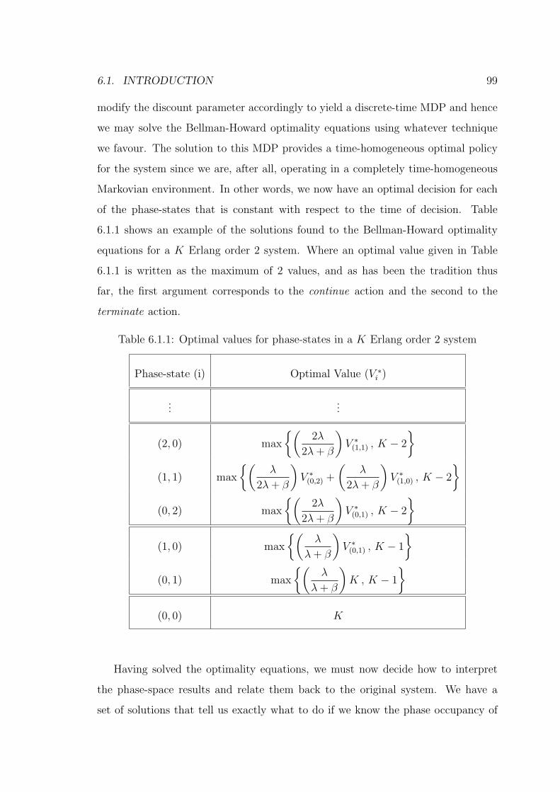
6.1. INTRODUCTION 99
modify the discount parameter accordingly to yield a discrete-time MDP and hence
we may solve the Bellman-Howard optimality equations using whatever technique
we favour. The solution to this MDP provides a time-homogeneous optimal policy
for the system since we are, after all, operating in a completely time-homogeneous
Markovian environment. In other words, we now have an optimal decision for each
of the phase-states that is constant with respect to the time of decision. Table
6.1.1 shows an example of the solutions found to the Bellman-Howard optimality
equations for a K Erlang order 2 system. Where an optimal value given in Table
6.1.1 is written as the maximum of 2 values, and as has been the tradition thus
far, the first argument corresponds to the continue action and the second to the
terminate action.
Table 6.1.1: Optimal values for phase-states in a K Erlang order 2 system
Phase-state (i) Optimal Value (V ∗i )
......
(2, 0) max
{(
2λ
2λ + β
)
V ∗(1,1) , K − 2
}
(1, 1) max
{(
λ
2λ + β
)
V ∗(0,2) +
(
λ
2λ + β
)
V ∗(1,0) , K − 2
}
(0, 2) max
{(
2λ
2λ + β
)
V ∗(0,1) , K − 2
}
(1, 0) max
{(
λ
λ + β
)
V ∗(0,1) , K − 1
}
(0, 1) max
{(
λ
λ + β
)
K , K − 1
}
(0, 0) K
Having solved the optimality equations, we must now decide how to interpret
the phase-space results and relate them back to the original system. We have a
set of solutions that tell us exactly what to do if we know the phase occupancy of
100 CHAPTER 6. PHASE-SPACE MODEL – ERLANG SYSTEM
the outstanding particles, and yet the original system that we are endeavouring to
understand has only knowledge of whether or not particles have arrived.
6.2 Existing Phase-Space Techniques
PH distributions have often been used in the modelling literature to extend simple
exponential models to more complex models without losing computational tractabil-
ity. Sethuraman and Squillante [80] construct a parallel server queuing model using
PH service times and Markovian Arrival Process (MAP) arrivals. A MAP is a pro-
cess extension of PH distributions, see for example Latouche and Ramaswami [58]
for more details. Bean, Kontoleon and Taylor in [10] modify an ordinary branching
process to enable non-exponential branch lengths, again using MAPs.
To this author’s knowledge however, the idea of expanding the state-space of a
system using a PH representation, solving an MDP on this new system, and then
mapping this information back to the original system in a sensible way has rarely
appeared in the context of decision processes to date. This approach is somewhat
the converse of a traditional partially observable MDP problem. A POMDP assumes
that the true model includes the expanded states, but the decision maker may not
have access to this information. The intention is therefore to ensure the POMDP
make as similar decisions as possible to the MDP where the expanded states are in
fact visible, as in Kaelbling, Littman and Cassandra [53]. He, Jewkes and Buzacott
[37] present an inventory production system where PH distributions are used to
model aspects such as production times. Optimal policies are derived using phase
occupancy knowledge which is not available in the original system. Heuristics are
then provided to approximate these optimal policies in the original system, that is,
to make the original system behave as though the phase information is available.
Our situation is also one where the model has additional information that is not
available in the original problem. Our aim, however, is to in some way shield this
information while still taking advantage of the knowledge gained from the underlying
phase-space in the model. The two notable attempts at this task come from Younes

6.2. EXISTING PHASE-SPACE TECHNIQUES 101
and Simmons [96] and Younes [95], both in the field of decision processes in the
realm of artificial intelligence. As such, the processes on which the papers focus
differ significantly from the race we consider here. Nevertheless, we will give a brief
discussion on the main ideas contained in each and how they apply to the race,
before highlighting where the more advanced of the two fails, not just for the race,
but fundamentally.
Younes and Simmons [96] offer a simulation based approach in their first attempt
at a solution to a time-dependent decision process using PH distributions. To put
their solution technique into the context of the race, suppose a visible transition
occurs. If continue is selected at this decision epoch, the following phase transitions
are simulated and a new decision epoch is made available each time a simulated
phase transition occurs. This technique essentially maps the original system to that
of the model with the expanded state-space, providing extra decision epochs than
were previously available in the real system. While this technique may appear to
be a reasonable practical solution to the decision process, there is an obvious flaw.
Consider the time-dependent optimal policy shown in Figure 5.2.1 with threshold
time t = 512
for level 2 of that system. It is possible, following the technique outlined
by Younes and Simmons, that a simulated phase transition, or combination of them,
can lead to the belief that it is best to continue the process while the absolute time
is less than the threshold. Conversely, a lack of simulated phase-transitions can
lead to the belief that it is best to terminate the process after the threshold time
t. Therefore, as the resulting policy from the simulated phase transitions can lead
to sub-optimal decisions, the policy itself must be sub-optimal. Let κ denote this
randomized policy determined by phase transition simulation. Figure 6.2.1 shows
the expected value received from such a simulation under this policy, V κ2 (s), in
comparison with the optimal value for state 2 of our standard Erlang example,
demonstrating the sub-optimal behaviour of the randomized policy.
In a later paper, Younes [95] notes that the phases do not correspond to physical,
and hence observable, features in the real world. By solving the problem as if the
phases are observable, as in [96], we ignore the observation model of the actual

102 CHAPTER 6. PHASE-SPACE MODEL – ERLANG SYSTEM
0 0.1 0.2 0.3 0.4 0.5 0.6 0.7 0.8 0.9 11.5
1.6
1.7
1.8
1.9
2
2.1
2.2
Comparison of Expected Values for Different Policies
s
Exp
ecte
d V
alue
Optimal: V2*(s)
Random: V2κ(s)
Figure 6.2.1: Comparison of expected values for optimal and randomized policies
process. He proposes a phase tracking model which we will describe using the
notation and framework we have given for the phase-space model of the race. Figure
6.2.2 gives a guideline summary of the phase tracking model of Younes [95]. We
include the summary to provide the reader with an outline of the steps involved in
constructing the model and solving for optimality, before elaborating on the steps
in greater detail. The summary in Figure 6.2.2 assumes an appropriate phase-space
has been constructed for the original model, where the phase-space for the Erlang
race is outlined in Section 6.1.
Consider the Markov chain with transitions defined by an infinitesimal generator
Q0. From Cinlar [21], at any time s ≥ 0, transient analysis of the Markov chain
via solution of the Kolmogorov differential equations tells us that the probability of
being in each of the states i ∈ S at time s, p(s) = [pi(s)], is given by
p(s) = p(0)eQ0s.
Therefore, it is possible to calculate a belief distribution over the phase-space at all
times s ≥ 0. The method in Younes [95], from an algorithmic perspective, specifies

6.2. EXISTING PHASE-SPACE TECHNIQUES 103
The phase tracking model.
1. Choose a level of the phase-space.
2. Choose an action available to the current level.
3. Value each phase-state of the current level according to the QMDP
valuation technique of [59].
4. Calculate the probabilities that each of the phase-states of the current
level are occupied at any given decision epoch.
5. Using the occupancy probabilities, mix the phase-state values to con-
struct the expected value of applying the chosen action in the current
level at any given decision epoch.
6. Repeat steps 2–5 for all available actions in the current level to deter-
mine the optimal action to take in the current level at any decision
epoch.
7. Repeat steps 1–6 for all levels of the phase-space.
Figure 6.2.2: Guideline summary of the phase tracking model
calculation of a belief distribution when a new visible decision epoch is reached. This
belief distribution tells the decision maker the probability distribution of phase-state
occupancy of the underlying phase-space at the decision epoch s.
The determination of action selection at each decision epoch in Younes [95] is
based on the QMDP value method from Littman, Cassandra and Kaelbling [59]. To
explain this value method, suppose we know that we are occupying state B of an
unmodified system at decision epoch s, and that state B has associated with it
some number of phase-states in the phase-space model, bi ∈ B. For each action a
available for selection in B at time s, we value each of the underlying phase-states bi
individually by forcing action a to be selected in bi and solving the MDP on the rest
104 CHAPTER 6. PHASE-SPACE MODEL – ERLANG SYSTEM
of the phase-space, allowing optimal behaviour in all other phase-states. This results
in a value for each of the phase-states bi corresponding to a particular action a, which
we will denote V abi,Q
, indicating that we have used the QMDP valuation method. Note
that these values will be time-independent, as we are solving the Bellman-Howard
optimality equations with just a slight modification of action selection in a single
phase-state.
Continuing with the technique given in [95], we then calculate the phase oc-
cupancy probability that each of the phase-states is occupied at time s, that is,
P [bi occupied at s|B occupied at s]. For each action available in B, we may use the
phase occupancy probabilities and the values for each of the phase-states to give an
expected value for state B in the original system at time s for the chosen action
a. We will denote this expected value Y aB(s), where we have substituted the tradi-
tional notation for value, V , for Y indicating the valuation is found using Younes’
technique. This expected value at s when action a is selected in B is given by
Y aB(s) =
∑
bi∈B
P [bi occupied at s|B occupied at s] V abi,Q
.
Once we have performed this for all available actions, to behave optimally in B at
time s we simply choose the action that provides the greatest expected value at s,
where this optimal value in B at s is given by
Y ∗B(s) = max
a{Y a
B(s) }.
Relating this work to the race, suppose that we have Q0 describing the natural
transitions of the phase-space when continue is selected. Assume that the process
begins in phase-state 1, (K, 0, . . . , 0), at time 0 and that we have a decision epoch
at s ≥ 0 where the system is known to be in level k. At this decision epoch,
we have two actions available, continue and terminate. Therefore we have V ci,Q as
the value in phase-state i ∈ Lk when the MDP of the phase-space is solved for
optimal behaviour while forcing the continue action in phase-state i. Trivially, the
corresponding termination value V ti,Q = k for all phase-states i ∈ Lk. Using the
technique outlined in [95] we can then calculate Y cLk
(s), the continuation value for

6.2. EXISTING PHASE-SPACE TECHNIQUES 105
level k, as
Y cLk
(s) =∑
i∈Lk
e1eQ0se′
n(i)∑
j∈Lk
e1eQ0se′
n(j)
V ci,Q, (6.2.1)
for all s ≥ 0, where eℓ is a row vector of zeros with a 1 in the iℓth position and
e1eQ0se′
n(i)∑
j∈Lk
e1eQ0se′
n(j)
(6.2.2)
gives the normalized probability that phase-state i ∈ Lk is occupied at time s
conditional on the knowledge that level k is occupied. To determine the optimal
expected value and hence action at all decision epochs, we simply compare Y cLk
(s)
with the termination value in level k and choose the action that gives rise to the
higher of the two possibilities. That is, we find a potentially time dependent optimal
value Y ∗Lk
given by
Y ∗Lk
(s) = max{Y cLk
(s) , k}, (6.2.3)
where the first element, Y cLk
(s), given in equation (6.2.1), corresponds to continuing
the process and the second corresponds to termination.
Nevertheless, there is a subtle, but definite, flaw in the use of the QMDP value
method as used in this situation. Considering level K−1 of our phase-space model,
equation (6.2.3) is in fact equivalent to the optimal value for state K − 1 given
in equation (5.2.12) found earlier via direct solution of the value equations. We
will show this in detail when we introduce our own phase-space technique, as it is
identical to the technique outlined by Younes for this particular level. To notice
the flaw, we must observe the system at a lower level and so let us consider level
K−2. For ease of demonstration, we will specifically consider level 1 of our standard
K = 3 order 2 Erlang system. Figure 6.2.3 shows the optimal values found in this
level using the value equations derived earlier and those found using the Younes
QMDP technique for this particular system.
We see in Figure 6.2.3 that the two techniques, while resulting in the same net
overall optimal policy, produce differing optimal expected values. The explanation

106 CHAPTER 6. PHASE-SPACE MODEL – ERLANG SYSTEM
0 0.1 0.2 0.3 0.4 0.5 0.6 0.7 0.8 0.9 11
1.1
1.2
1.3
1.4
1.5
1.6
1.7
1.8
1.9
2Comparison of Optimal Expected Values using Different Techniques
s
V1* (s
)
Value EquationsYounes
Figure 6.2.3: Comparison of techniques for state/level 1
as to the cause of this difference lies in the use of the QMDP valuation method, where
the phase-state values are found by forcing an action in a single phase-state and then
solving the MDP on the phase-space, allowing optimal actions in every other phase-
state of the model. In our particular example, there are two phase-states in level
2, (1, 0) and (0, 1). For the given system parameters, Table 6.1.1 gives V ∗(1,0) = 2,
indicating terminate, and V ∗(0,1) = 2.25, indicating continue. When we consider a
phase-state in level 1, we force it to choose continue but then allow the rest of the
phase-states to behave optimally when solving the MDP. Thus, the phase state sees,
upon hitting level 2, a terminate action and a continue action. It is the two values
caused by these differing actions that are effectively probabilistically mixed based
on the likelihood of hitting level 2 in either of those phase-states when solving the
Bellman-Howard optimality equations. Figure 6.2.4 shows the effective mixture of
the values produced by these two actions and hence the expected value of level 2 as
seen by a phase-state of level 1, labelled Younes in the plot. We have also included
the optimal expected value for comparison.
The main point here is that when considering the valuation of level 2, the true

6.2. EXISTING PHASE-SPACE TECHNIQUES 107
0 0.1 0.2 0.3 0.4 0.5 0.6 0.7 0.8 0.9 11.5
1.6
1.7
1.8
1.9
2
2.1
2.2
Expected Value of Level 2 as seen from Level 1
s
V2* (s
)
OptimalYounes
Figure 6.2.4: Expected optimal value of level 2 as seen from level 1
optimal policy was achievable. As soon as focus shifts to a lower level, by using
the QMDP valuation we lose this as we can no longer enforce the same behaviour in
both phase-states of level 2 at every epoch. In fact, this value relies on being able to
see which phase-state is hit upon arrival to level 2 and hence make an appropriate
optimal decision for that phase-state which is not available to the decision maker
in the original system. As such, the valuation of level 2 from lower levels is greater
than the optimal value we know to be true. Therefore, as shown in Figure 6.2.3 we
see that the Younes technique achieves a greater, or possibly equal, optimal value,
but it does this by utilizing information that should not be available.
The resulting optimal policy in level 1 remains the same in both instances given
for our particular example. This is not always the case, however, and it is possible to
construct systems where the higher value in the Younes valuation technique results
in different optimal decisions to that of the original system found through solution of
the value equations. Therefore, the resulting optimal policy found using the Younes
valuation is, in fact, sub-optimal for these systems.
In the following section we introduce our own phase-space technique. It is similar

108 CHAPTER 6. PHASE-SPACE MODEL – ERLANG SYSTEM
to that described in Younes [95], in that it is based on the phase-occupancy theme,
however we address the issue of inconsistent valuation of certain levels. The incon-
sistencies, as demonstrated in Figure 6.2.4, centre around the arrival at threshold
levels and so we pay particular attention to the valuation process in these instances.
6.3 Our Phase-Space Technique
In an effort to make the phase-space model more realistic in comparison with the
original model, we introduce a new valuation technique. In the original model, at
each decision epoch s the decision maker must choose a single action. Therefore,
in our phase-space technique we wish to replicate this behaviour. We define a new
property of phase-states such that if the prescribed optimal action for all phase-states
within a level is the same action from an MDP perspective, then the phase-states
are action-consistent. This has the direct result that, if the phase-states of a level
are action-consistent, we will find that the optimal policy for that level is time-
independent. When valuing phase-states of a particular level for a given action we
must ensure that the phase-states of all other levels are action-consistent. This is
how the decision maker should see the system as there is no definite knowledge of
phase-occupancy. By valuing the phase-states in this manner, we will now have to
consider the hitting time at action-inconsistent (threshold) levels more carefully to
ensure that an action-consistent view of them is seen in the valuation process. As
we will see, this corrects the fundamental flaw in Younes’ technique and results in a
technique that gives an equivalent valuation to that of the integral value equations
given in Chapter 5 for the Erlang race.
We denote the value of a phase-state i ∈ Lk when action a is selected at decision
epoch s, under our action-consistent valuation process, as V ai,AC(s). To calculate this
value, we must look at all levels other than Lk, on which Lk depends, to see if they
are action-consistent, that is, time-independent. If so, then we force action a in all
of the phase-states in Lk and solve for the values for the resulting MDP using the
Bellman-Howard optimality equations.

6.3. OUR PHASE-SPACE TECHNIQUE 109
Suppose, however, that a single level, Lm say, on which Lk is dependent has
a time-dependent optimal policy. This means that the phase-states of Lm are not
action-consistent and so we must carefully value the phase-states in Lk. Also, sup-
pose for simplicity that Lm has a single threshold time at which point it changes
from one action to another. When valuing phase-state i ∈ Lk, we must consider
the distribution of the hitting time at Lm and by the optimality principle we must
behave optimally upon hitting Lm. If it hits before the threshold, then we force
all phase-states of Lm to select the same action, dictated by the optimal policy for
epochs before the threshold time and similarly for hitting after the threshold time.
Therefore, we ensure an action consistent view of Lm from the perspective of the
decision maker. Note that our notation, V ai,AC(s) is dependent on the absolute time
of decision epoch, s, as the time at which we value a phase-state has a clear bearing
on the likelihood of hitting an action-inconsistent (time-dependent) level before or
after a threshold time. Once we have the action-consistent values of all of the phase-
states of a given level for all available actions, we can proceed as in [95]. Figure 6.3.1
provides a guideline summary of the steps involved in implementing our phase-space
technique.
Utilizing our AC valuation method, let us denote the value of a phase-state i
under selection of action a at decision epoch s, V ai,AC(s). Therefore we define
V aLk
(s) =∑
i∈Lk
e1eQase′
n(i)∑
j∈Lk
e1eQase′
n(j)
V ai,AC(s) (6.3.1)
to be the value of the process in level k under selection of action a at decision epoch
s. We have used the phase occupancy probabilities as defined in equation (6.2.2),
where Qa is the infinitesimal generator of the phase-space when action a is selected.
The optimal value of a level at decision epoch s is given by
V ∗Lk
(s) = maxa{V a
Lk(s) }, (6.3.2)
At this point, to study the phase-space technique in more detail we return to
the Erlang race. In this example, we will show that when using the AC valuation

110 CHAPTER 6. PHASE-SPACE MODEL – ERLANG SYSTEM
The phase-space technique.
1. Choose a level of the phase-space.
2. Choose an action available to the current level.
3. Value each phase-state of the current level according to the action-
consistent valuation technique.
4. Calculate the probabilities that each of the phase-states of the current
level are occupied at any given decision epoch.
5. Using the occupancy probabilities, mix the phase-state values to con-
struct the expected value of applying the chosen action in the current
level at any given decision epoch.
6. Repeat steps 2–5 for all available actions in the current level to deter-
mine the optimal action to take in the current level at any decision
epoch.
7. Repeat steps 1–6 for all levels of the phase-space.
Figure 6.3.1: Guideline summary of the phase-space technique
method, we may simplify the process of valuation for phase-states of certain levels
by exploiting properties of the phase-space. These potential exploitations are first
encountered and described in Section 6.3.4. While the phase-space technique is
valid without these simplifications, the summary of the technique in Section 6.4
incorporates them to provide a solution technique that is as computationally simple
as possible. The phase-space technique is studied in more detail in Chapter 7, where
the applicability of the technique and the simplifications exploiting the phase-space
are discussed for general processes.

6.3. OUR PHASE-SPACE TECHNIQUE 111
6.3.1 Level K
As we are interested in a level based policy, due to the nature of the original system,
we begin by implementing this technique in a top-down approach with respect to
level for reasons that will become evident as we progress. Even though it is trivial,
we once again for completeness begin in level K. When we choose to continue in the
only phase-state of level K, (0, 0, . . . , 0), there are no further decision epochs and so
no reward can be received. We can deduce from equations (6.3.1) and (6.3.2) that
V ∗LK
(s) = max{0 , K},
= K,
for all decision epochs s ≥ 0.
6.3.2 Level K − 1
Now, when considering level K − 1, all higher levels have an action-consistent op-
timal policy. Therefore, we can calculate the continuation values for the phase-
states in LK−1 using the Bellman-Howard optimality equations, which assume time-
independence, forcing the continue action in all phase-states of LK−1 for action-
consistency. We need not specifically calculate the termination values individually
in each of the phase-states, as we can simply compare the resulting level continuation
value with the level termination value as in equation (6.3.2).
Written in lexicographic order, the first phase-state in LK−1 is (1, 0, . . . , 0), the
second is (0, 1, . . . , 0) and so forth to the pth (last) phase-state (0, 0, . . . , 1). For nota-
tional convenience, we also label these as phase-states r = 1, 2, . . . , p corresponding
to the sequence number of the phase-states in the lexicographic ordering within level
K − 1. Using the optimality equations with the terminate action disabled in level
K − 1, we find that
V ci,AC(s) = K
(
λ
λ + β
)p−(r−1)
for all phase-states i ∈ LK−1.

112 CHAPTER 6. PHASE-SPACE MODEL – ERLANG SYSTEM
A decision maker supplied with a decision epoch at s can make use of these
underlying continuation values using probabilistic mixing as defined in equation
(6.3.1). That is, although not knowing for sure which of the phases are actually
occupied at s, the continuation values can be weighted with the likelihood that each
phase-state is occupied at s. This will yield an expected continuation value in the
current level, to which the value received for termination can be compared and the
optimal decision made accordingly.
When it comes to phase-state occupancy probabilities, it can be shown that
e1eQ0se′
n(i)∑
j∈LK−1
e1eQ0se′
n(j)
=
(λs)(r−1)
(r − 1)!p∑
j=1
(λs)j−1
(j − 1)!
for all i ∈ LK−1 where r again corresponds to the sequence number of phase-state i
in the lexicographic ordering within level K − 1.
Therefore, using equation (6.3.1) we find the continuation value in LK−1 at de-
cision epoch s,
V cLK−1
(s) =∑
i∈LK−1
e1eQ0se′
n(i)∑
j∈LK−1
e1eQ0se′
n(j)
V ci,AC(s)
=
p∑
r=1
(λs)(r−1)
(r − 1)!p∑
j=1
(λs)j−1
(j − 1)!
K
(
λ
λ + β
)p−(r−1)
= K
(
λ
λ + β
)p
p∑
r=1
(λs)(r−1)
(r − 1)!
(
λ + β
λ
)(r−1)
p∑
j=1
(λs)j−1
(j − 1)!

6.3. OUR PHASE-SPACE TECHNIQUE 113
= K
(
λ
λ + β
)p
p∑
r=1
((λ + β)s)(r−1)
(r − 1)!p∑
j=1
(λs)j−1
(j − 1)!
= K
(
λ
λ + β
)p(ξ(p,λ+β)(s)
ξ(p,λ)(s)
)
.
Hence the optimal value at decision epoch s, from equation (6.3.2), is given by
V ∗LK−1
(s) = max
{
K
(
λ
λ + β
)p(ξ(p,λ+β)(s)
ξ(p,λ)(s)
)
, K − 1
}
which is equivalent to the optimal value for state K − 1 given in equation (5.2.12)
and found via direct solution of the value equations. We can therefore make all of
the same claims regarding conditions for a time-dependent policy and location of
threshold as in Section 5.2.2.
We can also identify time-dependent optimal policies directly from the continua-
tion values of the phase-states. Suppose within a level there are phase-states whose
value for continuation is less than the termination value for the level and there are
also phase-states whose continuation is greater than the termination value. The
optimal action to take in some of the phase-states is terminate while in others it
is continue from an MDP perspective. The phase-states of the level are there-
fore not action-consistent and the level will involve a time-dependent policy. This
equates to the scenario of directly solving the MDP for this level and above us-
ing the Bellman-Howard optimality equations, as in Table 6.1.1 for order 2 Erlang
systems, and finding that some phase-states have an optimal decision of terminate
while others specify continue within the same level. We know from experience that
a time-dependent policy for our problem is where we terminate for earlier decision
epochs and then after some threshold we find that it becomes optimal, should a
decision epoch be made available, to continue the process. Thus, those that specify
termination will occur earlier in the ordering in a single block, followed by those
that specify continuation in a second block of phase-states.
For the decision epoch s = 0, the phase-occupancy probabilities tell us that,
conditional on being in the current level, we must be occupying the first phase-state,

114 CHAPTER 6. PHASE-SPACE MODEL – ERLANG SYSTEM
(1, 0, . . . , 0), with probability 1. This is intuitive as we have allowed no time to pass,
and hence no transitions can have occurred, and so we must be in the first phase-
state of the level. Similarly, if we consider a decision epoch s→∞, then conditional
that we are still in the current level, all other transitions must have occurred and so
we are just waiting for the last possible transition to exit to the next level and thus
must be occupying the last phase-state with probability 1. Recall Figure 5.2.1 which
shows the continuation and termination values for level 2 in our standard example
for a range of decision epochs s. At s = 0 we see that the continuation value is
1.6875 while the termination value is 2 and so the optimal decision is to terminate
the process. With these system parameters, using Table 6.1.1, we have V ∗(1,0) =
max{1.6875 , 2} = 2 where the first argument to the max operator corresponds to
the continuation value in phase-state (1, 0). We can therefore think of the optimal
value of the first phase-state as the optimal decision to make at s = 0. Although
it is not shown in Figure 5.2.1, there is an asymptote of the continuation value at
2.25 and thus the optimal decision is to continue the process as the absolute time of
the decision epoch increases to ∞. Again, using Table 6.1.1, we have that V ∗(0,1) =
max{2.25 , 2} = 2.25 and so the optimal decision in this phase-state is to continue
the process. Therefore, we may also think of the optimal value of the last phase-
state as the limiting value as we let our decision epoch tend to infinity. If these
two optimal values prescribe a different optimal decision, as in our specific example,
then the resulting optimal policy for the level as a whole will be time-dependent.
As a brief summary of the steps we have followed using our phase-space technique
in level K−1, we firstly find the continuation values of the phase-states of level K−1.
We do this by simply disabling the terminate action in these phase-states and solve
the Bellman-Howard optimality equations in levels K − 1 and K. As these levels
form a standard MDP, the continuation values themselves are time-independent. We
then use the phase-occupancy probabilities defined in equation (6.2.2) to probabilis-
tically weight the continuation values, resulting in a time-dependent continuation
value as defined in equation (6.3.1). Then, using equation (6.3.2), we compare this
continuation value to that of an immediate termination value to determine an overall

6.3. OUR PHASE-SPACE TECHNIQUE 115
optimal value and hence optimal policy for all decision epochs s ≥ 0.
The primary reason we were able to reconstruct the optimal value functions
using the phase-space model is that the phase-states of the level directly above were
action-consistent and hence the level had a time-independent policy. As such, we
simply used the Bellman-Howard optimality equations with terminate disabled in
all phase-states of LK−1, which take into account the time taken to reach the next
level where we see a new decision epoch and behave optimally. Level K, however,
consisted of a single phase-state, and so now we proceed to investigate the situation
where the next level up in the system consists of more than one phase-state and
particularly when the optimal decisions in all of phase-states of the next level are
not all the same.
6.3.3 Level K − 2
We now consider the level where there are two outstanding particles yet to arrive at
the destination. In level K − 2, there are p(p+1)2
phase-states and recall that there
are p phase-states in level K−1. We begin by considering the situations where level
K − 1 has a time-independent optimal policy before considering the more involved
scenario where its optimal policy is time-dependent.
Let us first consider a system such that level K− 1 has a time-independent, and
thus action-consistent, optimal policy where continue is always selected. Note that
this corresponds to a threshold in level K − 1 of t = 0 using our earlier convention.
Being this particular time-independent policy means that the optimal decision in
every phase-state of this level, when solving the MDP of the phase-space model, is
to continue the process. Focusing now on the phase-states of level K−2, to calculate
their continuation values we need only take into account the expected present value
of the eventual termination reward, and hence the hitting time distribution of level
K, the all arrived level. Recall, however, that the continuation value in any phase-
state is effectively the present value, upon arriving in that phase-state, of the possible
future reward for termination. Therefore, to maintain a single level look ahead where
possible, we can in fact equivalently calculate the continuation values in level K − 2

116 CHAPTER 6. PHASE-SPACE MODEL – ERLANG SYSTEM
by considering the hitting time distribution of level K−1. That is, we can construct
continuation values by looking ahead a single level, where that level itself also looks
ahead a single level, as in Bellman’s optimality principle.
The other time-independent optimal policy in level K − 1 is where all phase-
states specify immediate termination, corresponding to a threshold time t = ∞.
In this case, the continuation values in level K − 2 are automatically based on the
hitting time distribution of level K − 1 at which point it is optimal to terminate
the process. In summary, to calculate the continuation values for the phase-states
of level K − 2, we may use the Bellman-Howard optimality equations on the phase-
space model for levels K − 2, K − 1 and K with the termination action disabled in
level K − 2, provided that the optimal policies for all levels above level K − 2 are
time-independent.
Up until this point, whenever we have mentioned the solution of the Bellman-
Howard equations, we have meant the equations resulting from the discrete MDP
resulting from uniformization of the transition rate matrices. We now give the
direct representation of the optimality equations in continuous-time, that enables
us to consider time-dependent optimal policies in level K − 1 and their effect on
level K − 2. The optimality equations for all states i ∈ S may be written as
V ∗i = max
a∈A
{
γai +
∑
j∈S
V ∗j
∫ ∞
0
e−βθdP aij(θ)
}
, (6.3.3)
where P aij(θ) is the probability that if the system is in state i and action a is selected,
then the next decision epoch will be in state j at or before time θ. For our expanded
phase-space model, we can re-write equations (6.3.3) in terms of continuation and
termination values for i ∈ Lk as
V ∗i = max {V c
i , k} ,
where
V ci =
∑
j∈S
V ∗j
∫ ∞
0
e−βθdPij(θ), (6.3.4)
noting that we have dropped the specific action reference in the probability transition
function. By definition of the probability transition function Pij(θ), the only non-

6.3. OUR PHASE-SPACE TECHNIQUE 117
zero terms in the summation of equation (6.3.4) correspond to the phase-states j
that can be reached in a single transition from phase-state i. In this situation, all
transitions are exponential and it is not hard to show that the optimal values found
in this manner are equivalent to those found using the uniformization technique.
In our level based model, however, we are not necessarily interested in seeing
every possible transition. In fact, we have seen thus far that we are predominantly
interested in seeing when we hit a specific level. Particularly, when considering a
phase-state i in level K − 2, we have said that to calculate its continuation value
we need to know the hitting time distribution of the next level above, level K − 1.
Modifying the standard optimality equations, we may write an equivalent set of
continuation values to those given in equations (6.3.4). For i ∈ Lk, focusing on the
hitting times of a level of interest, Lm say, where m > k, we have that
V ci =
∑
j∈Lm
V ∗j
∫ ∞
0
e−βθdPLm
ij (θ). (6.3.5)
Here, PLm
ij (θ) defines the probability distribution of first hitting phase-state j ∈ Lm
from phase-state i ∈ Lk at or before time θ. In the race, the process must eventually
hit level m and so, by summing over all phase-states in Lm, we are taking into
account all possible phase-state paths that may be taken from phase-state i to Lm.
Transitions between the phase-states of different levels, such as those from i ∈ Lk
to j ∈ Lm are generally no longer exponentially distributed. We nevertheless have
at our disposal a convenient representation of these probability transition functions,
as PH distributions.
Recall from Chapter 3 that a phase-type random variable is the time taken to
progress through the states of a finite-state evanescent Markov chain until absorp-
tion. By removing the rows and columns corresponding to level m (and above) from
our phase-space generator matrix Q0, we are left with a PH -generator matrix T m,
using the standard PH notation, that defines the time to absorption into level m.
Thus, given any starting state, we can calculate the first hitting time distribution
of level m. Unfortunately, with the standard PH representation there is no way to
distinguish between the phase-states of level m that the process actually enters. In

118 CHAPTER 6. PHASE-SPACE MODEL – ERLANG SYSTEM
the definition of the density function of a PH random variable,
f(x) = −αexp(Tx)Te,
we can think of the vector Te as the entry vector, in terms of transition rates, into
the absorption state. We, however, wish to know the rate at which each of our
phase-states in the level of interest are entered individually, instead of the level as
a whole. Therefore, we define τ j to be the entry vector into phase-state j ∈ Lm,
which can be found by removing the rows corresponding to phase-states in level m
from Q0 and letting τ j be the column corresponding to phase-state j.
In terms of the PH distributed hitting times on our level of interest, we can
reduce equations (6.3.5) to
V ci =
∑
j∈Lm
V ∗j
∫ ∞
0
−e−βθen(i)eTmθτ jdθ,
=∑
j∈Lm
V ∗j (−en(i))
∫ ∞
0
e(Tm−βI)θdθ τ j,
=∑
j∈Lm
V ∗j en(i) (Tm− βI)−1
τ j, (6.3.6)
for all i /∈ Lm where n(i) is the row number corresponding to state i in Tm and I is
the identity matrix of appropriate dimension. Here the last equation is justified by
the following argument. Consider the matrix A = Tm− βI. The n×n, say, matrix
Tm satisfies the diagonally dominant condition
|Tii| ≥n∑
j=1j 6=i
|Tij|, ∀i = 1, . . . , n,
as it is a PH -generator matrix. The matrix A is therefore strictly diagonally domi-
nant and we note that, as the diagonal elements of Tm are negative and β > 0, the
diagonal elements of A are strictly negative. A theorem due to McKenzie [62] states
that if a square matrix A is diagonally dominant and the diagonal is composed of
negative elements, then every eigenvalue of A has a negative real part and A is
stable, a property relating to systems of linear differential equations. Using Remark
2.4.5 on the proof of Theorem 2.4.3 of Latouche and Ramaswami [58], as A is stable,

6.3. OUR PHASE-SPACE TECHNIQUE 119
we have that limx→∞ eAx = 0 and thus A−1 exists and is given by
A−1 = −∫ ∞
0
eAxdx.
We can use equations (6.3.6) for all phase-states i ∈ LK−2 where our level of
interest is LK−1 provided that the optimal policy in level K−1 is time-independent,
that is, the phase-states are action-consistent. When this is the case, the calculation
of continuation values in level K−2 simply involves the optimal values in level K−1
propagated back and discounted accordingly. As such, the continuation values of
the individual phase-states in this scenario are also time-independent, a direct result
from the use of the Bellman-Howard optimality equations.
The more interesting system to analyze is such that there exists a non-zero and
finite threshold time t in level K − 1. In other words, the optimal policy in level
K−1 is time-dependent, specifying termination at or before the threshold time and
continuation after. Equations (6.3.5) do not suffice in this situation as we must now
take into account whether or not we hit LK−1 before or after the threshold time.
Hence, we must also consider the absolute time of the decision epoch, s, as this will
affect the probability of being able to arrive in LK−1 before the threshold time.
The structure for continuation values defined above for the time-independent
scenario, however, lends itself quite nicely to this considerable addition of complexity.
For our particular Erlang example, we may now write the continuation values for
phase-states i ∈ LK−2, under our action-consistent valuation method, as
V ci,AC(s) =
∑
j∈LK−1
[
(K − 1)
∫ max{s,t}
s
e−β(θ−s)dPLK−1
ij (s, θ)
+ V cj
∫ ∞
max{s,t}
e−β(θ−s)dPLK−1
ij (s, θ)
]
. (6.3.7)
Here, PLK−1
ij (s, θ) is the probability that if the system is in phase-state i ∈ LK−2
at decision epoch s, then the transition to the level of interest, LK−1, will be to
phase-state j ∈ LK−1 at or before time θ. As we are now considering the interval
from s to θ, we simply adjust the start of integration from 0 to s and make sure that
we are calculating the correct amount of discount, that is e−β(θ−s). The expected
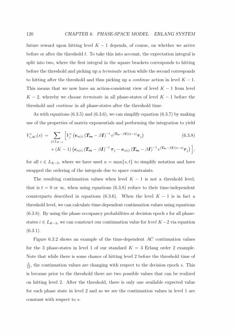
120 CHAPTER 6. PHASE-SPACE MODEL – ERLANG SYSTEM
future reward upon hitting level K − 1 depends, of course, on whether we arrive
before or after the threshold t. To take this into account, the expectation integral is
split into two, where the first integral in the square brackets corresponds to hitting
before the threshold and picking up a terminate action while the second corresponds
to hitting after the threshold and thus picking up a continue action in level K − 1.
This means that we now have an action-consistent view of level K − 1 from level
K − 2, whereby we choose terminate in all phase-states of level K − 1 before the
threshold and continue in all phase-states after the threshold time.
As with equations (6.3.5) and (6.3.6), we can simplify equation (6.3.7) by making
use of the properties of matrix exponentials and performing the integration to yield
V ci,AC(s) =
∑
j∈LK−1
[
V cj
(
en(i) (Tm− βI)−1 e(Tm−βI)(u−s)τ j
)
(6.3.8)
+ (K − 1)(
en(i) (Tm− βI)−1τ j − en(i) (Tm− βI)−1 e(Tm−βI)(u−s)τ j
)
]
,
for all i ∈ LK−2, where we have used u = max{s, t} to simplify notation and have
swapped the ordering of the integrals due to space constraints.
The resulting continuation values when level K − 1 is not a threshold level,
that is t = 0 or ∞, when using equations (6.3.8) reduce to their time-independent
counterparts described in equations (6.3.6). When the level K − 1 is in fact a
threshold level, we can calculate time-dependent continuation values using equations
(6.3.8). By using the phase occupancy probabilities at decision epoch s for all phase-
states i ∈ LK−2, we can construct our continuation value for level K−2 via equation
(6.3.1).
Figure 6.3.2 shows an example of the time-dependent AC continuation values
for the 3 phase-states in level 1 of our standard K = 3 Erlang order 2 example.
Note that while there is some chance of hitting level 2 before the threshold time of
512
, the continuation values are changing with respect to the decision epoch s. This
is because prior to the threshold there are two possible values that can be realized
on hitting level 2. After the threshold, there is only one available expected value
for each phase state in level 2 and so we see the continuation values in level 1 are
constant with respect to s.
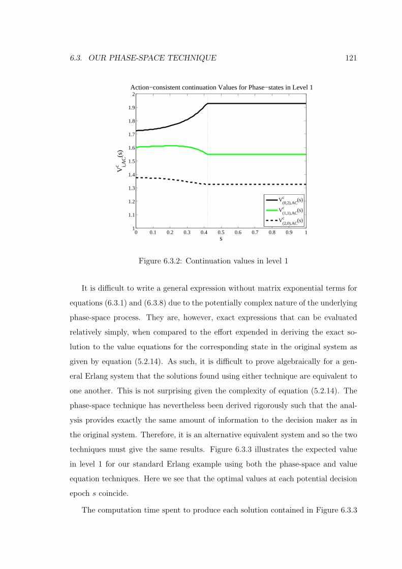
6.3. OUR PHASE-SPACE TECHNIQUE 121
0 0.1 0.2 0.3 0.4 0.5 0.6 0.7 0.8 0.9 11
1.1
1.2
1.3
1.4
1.5
1.6
1.7
1.8
1.9
2Action−consistent continuation Values for Phase−states in Level 1
s
Vi,A
Cc
(s)
V(0,2),ACc (s)
V(1,1),ACc (s)
V(2,0),ACc (s)
Figure 6.3.2: Continuation values in level 1
It is difficult to write a general expression without matrix exponential terms for
equations (6.3.1) and (6.3.8) due to the potentially complex nature of the underlying
phase-space process. They are, however, exact expressions that can be evaluated
relatively simply, when compared to the effort expended in deriving the exact so-
lution to the value equations for the corresponding state in the original system as
given by equation (5.2.14). As such, it is difficult to prove algebraically for a gen-
eral Erlang system that the solutions found using either technique are equivalent to
one another. This is not surprising given the complexity of equation (5.2.14). The
phase-space technique has nevertheless been derived rigorously such that the anal-
ysis provides exactly the same amount of information to the decision maker as in
the original system. Therefore, it is an alternative equivalent system and so the two
techniques must give the same results. Figure 6.3.3 illustrates the expected value
in level 1 for our standard Erlang example using both the phase-space and value
equation techniques. Here we see that the optimal values at each potential decision
epoch s coincide.
The computation time spent to produce each solution contained in Figure 6.3.3
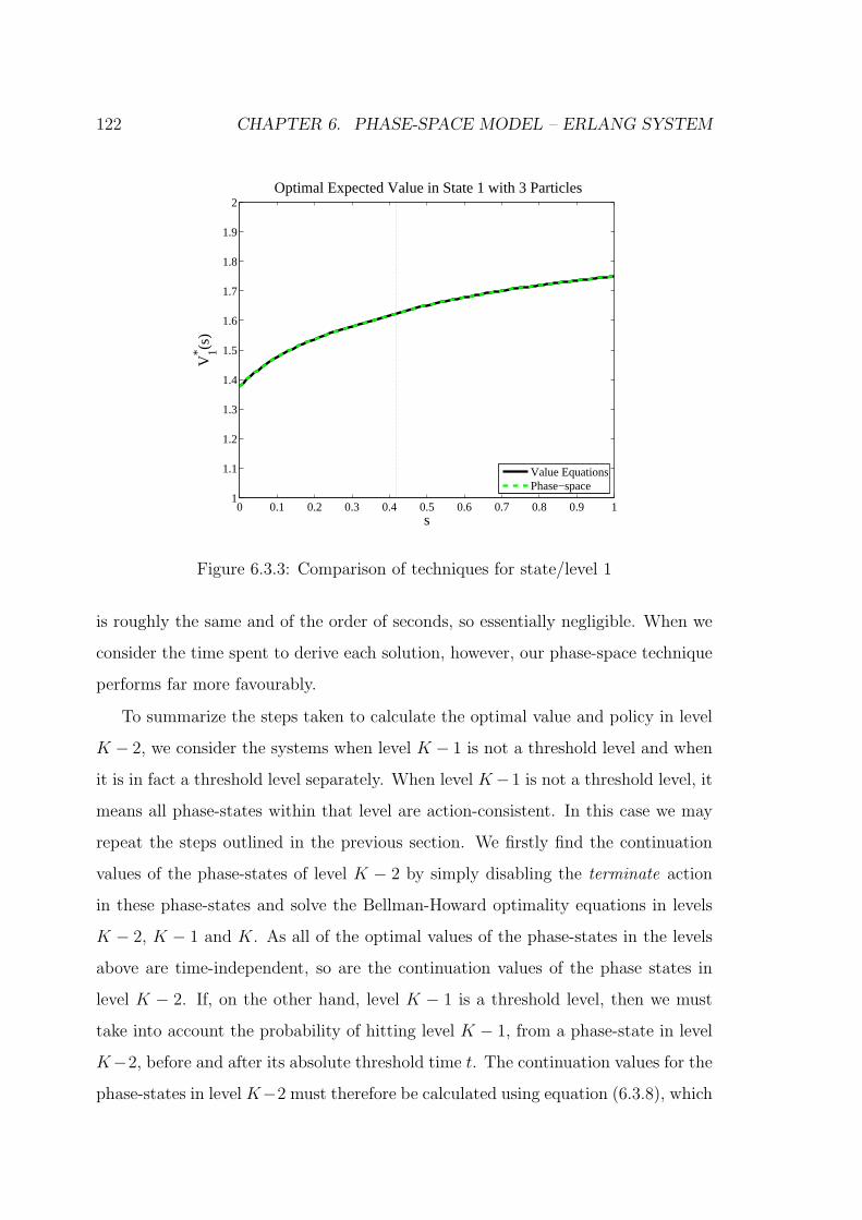
122 CHAPTER 6. PHASE-SPACE MODEL – ERLANG SYSTEM
0 0.1 0.2 0.3 0.4 0.5 0.6 0.7 0.8 0.9 11
1.1
1.2
1.3
1.4
1.5
1.6
1.7
1.8
1.9
2Optimal Expected Value in State 1 with 3 Particles
s
V1* (s
)
Value EquationsPhase−space
Figure 6.3.3: Comparison of techniques for state/level 1
is roughly the same and of the order of seconds, so essentially negligible. When we
consider the time spent to derive each solution, however, our phase-space technique
performs far more favourably.
To summarize the steps taken to calculate the optimal value and policy in level
K − 2, we consider the systems when level K − 1 is not a threshold level and when
it is in fact a threshold level separately. When level K−1 is not a threshold level, it
means all phase-states within that level are action-consistent. In this case we may
repeat the steps outlined in the previous section. We firstly find the continuation
values of the phase-states of level K − 2 by simply disabling the terminate action
in these phase-states and solve the Bellman-Howard optimality equations in levels
K − 2, K − 1 and K. As all of the optimal values of the phase-states in the levels
above are time-independent, so are the continuation values of the phase states in
level K − 2. If, on the other hand, level K − 1 is a threshold level, then we must
take into account the probability of hitting level K − 1, from a phase-state in level
K−2, before and after its absolute threshold time t. The continuation values for the
phase-states in level K−2 must therefore be calculated using equation (6.3.8), which
6.3. OUR PHASE-SPACE TECHNIQUE 123
will be time-dependent for all non-trivial threshold times t. Irrespective of whether
or not level K − 1 is a threshold level, we have now calculated the continuation
values for all of the phase-states of level K − 2. We then use the phase-occupancy
probabilities defined in equation (6.2.2) to probabilistically weight the continuation
values, resulting in a time-dependent continuation value for level K−2 as defined in
equation (6.3.1). Then, using equation (6.3.2), we compare this continuation value
to that of an immediate termination value to determine an overall optimal value for
level K − 2 and hence optimal policy for all decision epochs s ≥ 0.
6.3.4 Level K − 3
We have claimed already that our phase-space technique is more manageable than
the alternative solution of the nested integral value equations. One of our technique’s
major advantages, however, is actually evident for those levels that are further than a
single level away from the highest threshold level. The construction of our technique
thus far, and the basic dynamic programming principle, maintains a single level look
ahead where possible, but this restriction is by no means necessary. It was included
as it simplifies the hitting time probabilities, when our goal is an analytic expression,
as the paths to the next level that require consideration are clearly shorter than to
any higher level. We will nevertheless demonstrate that situations may arise where
it is advantageous to look further ahead, specifically to a threshold level, in order
to maintain the analytic tractability of the solution technique.
Suppose firstly that the system parameters are such that level K − 1 is not a
threshold level and thus the optimal solutions to the phase-states in level K − 2
are time-independent. If we find that the phase-states in level K − 2 are action-
consistent, that is the overall optimal policy for level K − 2 is also not a threshold
policy, then we may solve for the continuation values in level K−3 by considering the
Bellman-Howard optimality equations with terminate disabled in level K− 3. Once
found, we can use these continuation values and the phase-occupancy probabilities
to construct the continuation value function for level K − 3, as in equation (6.3.1),
whereby we may determine the optimal policy for level K−3 using equation (6.3.2).
124 CHAPTER 6. PHASE-SPACE MODEL – ERLANG SYSTEM
Of course, it is possible for K − 2 to be a threshold level in its own right. When
this is the case, there will exist an absolute threshold time, which we will again
refer to as t, whereby hitting level K−2 before this threshold results in termination
whilst hitting after t results in continuation of the process. When solving for the
phase-state values in level K − 3, as we are considering a single level look-ahead to
a threshold level, we have already described the solution technique for this scenario.
We may simply re-write equation (6.3.7) with the references to level shifted down
by one, to give the continuation values for phase-states i ∈ LK−3 as
V ci (s) =
∑
j∈LK−2
[
(K − 2)
∫ max{s,t}
s
e−β(θ−s)dPLK−2
ij (s, θ)
+ V cj
∫ ∞
max{s,t}
e−β(θ−s)dPLK−2
ij (s, θ)
]
.
We can therefore follow all of the same steps as in the previous section when the
level above is a threshold level. As usual, this involves mixing the time-dependent
continuation values using phase-occupancy probabilities as in equation (6.3.1) in
order to determine the optimal policy for level K − 3 using equation (6.3.2).
When level K − 1 is not a threshold level and so its optimal policy is time-
independent, we have considered the cases where the resulting optimal policy in
level K − 2 is both time-independent and time-dependent. In either scenario, we
had previously developed a way to calculate the continuation value for a level using
only the information supplied from the level directly above.
Now let us consider the more interesting situation of a system such that level
K − 1 is a threshold level. To summarize, the phase-state continuation values in
level K−1 are time-independent but the value for level K−1, and also the optimal
policy, resulting from the phase-mixing process are time-dependent and we have a
threshold t. From equation (6.3.7) we know that the phase-state continuation values
in level K − 2 are therefore time-dependent, with an example of such values given
in Figure 6.3.2. Recall equation (6.3.5), for all i ∈ Lk,
V ci =
∑
j∈Lm
V ∗j
∫ ∞
0
e−βθdPLm
ij (θ),

6.3. OUR PHASE-SPACE TECHNIQUE 125
where the focus is on the hitting time of level m. The primary reason behind the
analytic tractability of our solution technique thus far is that the optimal value
found in phase-state j of the level of interest is time-independent and so appears
outside the integral. This in turn gives rise to time-independent continuation values
for the phase-states i ∈ Lk.
Given that the continuation values in phase-states of level K − 2 are time-
dependent, it is possible that their individual optimal values may also be time-
dependent. Therefore, using the idea behind equation (6.3.5) would actually require
the solution of
V ci (s) =
∑
j∈LK−2
∫ ∞
s
V ∗j (θ)e−β(θ−s)dP
LK−2
ij (s, θ), (6.3.9)
for all phase-states i ∈ LK−3. Although we have defined our transition probabilities
in terms of a PH distribution, we cannot use any of the simplifications of the integrals
used earlier, due to the potentially time-dependent nature of the optimal values in
level K − 2. The solution of equation (6.3.9) is hence akin to that of the integral
value equations described for the original system. In this situation, the use of the
phase-space technique provides little, if any, advantage over that of tackling the
direct value equations.
Let us however return to equation (6.3.7) which stated that for i ∈ LK−2, the
continuation values could be expressed by
V ci (s) =
∑
j∈LK−1
[
(K − 1)
∫ max{s,t}
s
e−β(θ−s)dPLK−1
ij (s, θ)
+ V cj
∫ ∞
max{s,t}
e−β(θ−s)dPLK−1
ij (s, θ)
]
.
where level K−1 is a threshold level. At this point we note that there is no necessary
restriction on phase-state i belonging to any level in particular, provided that it does
belong to a lower level than level K−1. A necessary restriction, however, is that level
K − 1 must be reachable at all times θ ≥ s, which is not an issue when considering
i ∈ LK−2 although we must take care when considering lower levels. For i ∈ LK−3,
if LK−2 specified terminate for some interval of the region of interest, then LK−1
would not be reachable in this interval and equation (6.3.7) would be insufficient.

126 CHAPTER 6. PHASE-SPACE MODEL – ERLANG SYSTEM
We may focus on the hitting time θ at LK−1, provided continue is the optimal
action at all times in the phase-states of LK−2. In such situations, we therefore
decide that, in the interest of analytic tractability, it is better to look from level
K − 3 directly to level K − 1, bypassing the time-dependent optimal continuation
values of the phase-states in level K − 2. In this manner, we can calculate the
continuation values for level K − 3 without the need for solution of complicated
integrals to achieve the same results as in the original system. In essence we have
just placed all the extra complexity in dPLK−1
ij (s, θ), which remains a simple PH -
type distribution. Figure 6.3.4 shows the expected value for level 0 at decision epoch
s for our standard Erlang K = 3 example using this approach and compares it with
the value equation approach of Chapter 5.
0 0.1 0.2 0.3 0.4 0.5 0.6 0.7 0.8 0.9 10.8
0.9
1
1.1
1.2
1.3
1.4
1.5
1.6
1.7
1.8Optimal Expected Value in State 0 with 3 Particles
s
V0* (s
)
Value EquationsPhase−space
Figure 6.3.4: Comparison of techniques for state/level 0
Once again we see that the optimal values for the different techniques coincide as
expected. Recall, however, that we had ceased our analysis of the value equations of
the original system by state K−3. Production of the plot for state 0 requires numer-
ical techniques to approximate a rather complicated integral. Using our phase-space
technique, we have an exact analytic expression without integrals, albeit containing

6.4. SUMMARY 127
matrix exponentials, and it is very fast to evaluate.
6.4 Summary
We choose to cease the specific level analysis here, not because the complexity has
grown out of control as with the original system, but rather because we have covered
all scenarios that may arise for our Erlang system. When solving the problem using
the phase-space model, we begin at the highest level and work down to the lowest,
using a dynamic programming approach.
Consider an arbitrary level of the race, Lk, where all higher levels have been
valued using our dynamic programming approach. If there is a sequence of levels
directly above the current level with each having one or more time-dependent op-
timal phase-state values, but all specify continue as their optimal action, then we
wish to exploit the properties of the phase-space and skip these levels. Define LT to
be the nearest level to the current level with no time-dependent optimal phase-state
values. If all levels between the current level and LT are action consistent, specifying
continue as their optimal action, we say that there is a valid continuation path from
the current level to LT . When a valid continuation path exists, we focus on the
hitting time of LT and bypass direct analysis of all levels in between.
When there are no levels between Lk and LT , that is LT = Lk+1, then there
must be a valid continuation path, as there are no levels in between the two to
prevent guaranteed passage. If Lk+1 is not a threshold level, then we solve for the
continuation values using the Bellman-Howard optimality equations with terminate
disabled in the current level. If it is a threshold level, then we must maintain an
action-consistent view of the process and thus we solve for the continuation values
of the current level using the AC valuation method, which incorporates the hitting
time distribution of the threshold level.
Note that for the race, the existence of LT is guaranteed, as LK will always be
a suitable candidate. The situation that a valid continuation path to LT cannot be
found implies the existence of a threshold level with time-dependent optimal phase-

128 CHAPTER 6. PHASE-SPACE MODEL – ERLANG SYSTEM
state values in between the current level and LT . In this case, we cannot focus solely
on LT and thus we revert to the standard focus on the level directly above and deal
with the complexity of the optimality equations.
It serves no useful purpose to focus on any levels that have time-dependent
phase-state values, threshold or not, as we lose the simple expressions for the in-
tegrals and hence the analytic tractability of our technique. As such, we avoid
such time-dependent phase-state values by implementing the aforementioned level-
skipping method. Once the continuation values have been found for the current
level, irrespective of the scenario regarding the other levels of the system, we use
equations (6.3.1) and (6.3.2) to solve for its optimal value and hence its optimal
policy. Figure 6.4.1 provides a concise algorithmic summary of the phase-space
technique applied to the race.
In the following chapter we formalize the phase-space technique, generalizing the
actual systems to which our technique can apply.

6.4. SUMMARY 129
V ∗LK
(s) = K for all s ≥ 0.
Set current level k ← (K − 1).
1. Observe all already valued levels.
Find LT .
If there exists a valid continuation path from Lk to LT ,
set focus level LF ← LT .
Else,
set focus level LF ← Lk+1.
2. Calculate the continuation values of all phase-states of Lk with direct
focus on LF using the AC valuation method.
3. Use phase-state occupancy probabilities to construct a continuation
value for Lk at all times.
4. Calculate the optimal value and policy for Lk at all times.
5. While Lk 6= L0, set current level k ← (k − 1) and return to Step 1.
Figure 6.4.1: Algorithmic summary of the phase-space technique for the race

Chapter 7
Phase-Space Model – General
Analysis
7.1 The Decision Process and Optimal Actions
In this chapter, we prove the validity of our phase-space model and its subsequent
optimality equations for a particular class of decision processes. Before we begin the
general analysis, however, we will require some defining properties of the decision
processes to which our model applies, together with some additional definitions
regarding aspects of optimal solutions.
We consider decision processes that are to be analyzed in continuous-time with
an infinite planning horizon. With regard to the actions available in each state for
controlling the process, the action space Ai associated with state i, for all i ∈ S,
is finite. This restriction is not too limiting, but it is necessary to guarantee that
an optimal value in a state is in fact achievable. We will be comparing policies
for the decision process via the expected discounted total reward metric. For the
class of processes under consideration, the time spent in any state, when any action
available to that state is selected, may be arbitrarily distributed. This duration,
however, may depend only on the state and the absolute time of the process when
the action is selected, and not on any prior history of the process.
An important restriction for the technique outlined herein is that the reward
131
132 CHAPTER 7. PHASE-SPACE MODEL – GENERAL ANALYSIS
structure of the decision process and the discounting is time-homogeneous. Without
this restriction, we would not be able to use any of the standard infinite horizon
solution techniques of continuous-time processes and hence the resulting optimality
equations are, in general, too complex for reasonable analysis. The aforementioned
classifications and restrictions therefore define our decision process, at its most com-
plex, as a time-inhomogeneous semi-Markov decision process, which we value using
the expected discounted total reward metric. The potential for time-inhomogeneity
in the process is a direct result of the generality we have allowed for the probability
distributions of the sojourn times in each of the states.
As usual, the goal for the decision process is to find a policy π ∈ Π such that the
expected present value of the process in state i ∈ S at decision epoch s is optimal, for
all states in S at all potential decision epochs s. Taking optimal to mean maximal
for our process, we wish to find π∗ such that V ∗i (s) = V π∗
i (s) ≥ maxπ∈Π {V πi (s)} for
all i ∈ S and s ≥ 0.
For the processes considered in this chapter, we restrict the policy class such that
a policy specifies an action to be selected in state i ∈ S at decision epoch s. This is in
contrast to the more general policies considered in Section 4.4.2 that permit delayed
action selection or the more complicated decisions of a sequence of actions mentioned
therein. This restriction is fairly standard in the Markovian process literature and
appears in Howard [43] when analyzing SMDPs. Allowing more complex policies,
while not invalidating the value equations derived in Section 7.4, complicates the
identification of the simplifications outlined in Section 7.5 substantially, the main
focal points of the phase-space technique.
Let us consider V ∗i (s), the optimal expected value for a particular state i ∈ S
as a function of the decision epoch variable s. The optimal action specified by the
optimal policy for state i may be dependent on the absolute time of the decision
epoch s and, in general, there may be multiple changes of optimal action as we vary
s. For s in the interval [0,∞), we break the optimal value function into its piecewise
components such that, in each piecewise interval, the optimal action specified by
the optimal policy is consistent. Define Ti to be the total number (possibly infinite)

7.2. PHASE-SPACE CONSTRUCTION 133
of piecewise action-consistent intervals for the decision epoch s. To denote the
endpoints of these intervals, define ti(ℓ) to be the ℓth absolute time of change in
optimal action, where ℓ = 0, 1, . . . , Ti with fixed boundary conditions of ti(0) = 0
and ti(Ti) = ∞. Therefore, under this formulation we have that for any decision
epoch s ∈ [ti(ℓ − 1), ti(ℓ)), for ℓ = 1, . . . , Ti, the optimal policy specifies a single
action, which we denote a∗i (ℓ), where a∗
i (ℓ) ∈ Ai.
Using the notation from Section 4.4 and the above process restrictions, we may
now write down some parameters to describe our general process. The state-space
of the system, which we will refer to as the original model, is S. For all states
i, k ∈ S, such that state k is a single state transition from state i, we have under
action a ∈ Ai a time-homogeneous continuously received permanence reward for
remaining in state i, ϕai , and a time-homogeneous impulse reward received upon
transitioning to state k, γaik. As we have assumed time-homogeneous discounting,
we have a constant decay rate β ≥ 0. We therefore have, using equations (4.4.3),
the optimal expected present value at decision epoch s in state i, assuming a∗ ∈ Ai
is optimal at epoch s, given by
V ∗i (s) =
∑
k∈S
∫ ∞
s
[(∫ θ
s
ϕa∗
i e−β(α−s)dα
)
+(
γa∗
ik + V ∗k (θ)
)
e−β(θ−s)
]
dP a∗
ik (s, θ), ∀i ∈ S and s ≥ 0, (7.1.1)
where we note the the optimal action a∗ at s may vary over the life of the process.
7.2 Phase-Space Construction
Equations (7.1.1) relate to the state-space, S, of the original model. Suppose now
that we replace the general probability distribution functions with their PH -type
distributions equivalents, or approximations if necessary. Having done this, we can,
for the moment, allow the decision maker to see phase-occupancy of all of the distri-
butions at any time. This effectively expands the state-space of the system to, as we
refer to it, a phase-space which we denote Sp, to distinguish it from the state-space
of the original model.

134 CHAPTER 7. PHASE-SPACE MODEL – GENERAL ANALYSIS
The phase-states of the phase-space are a representation of all possible feasible
combinations of phase-occupancies of all PH distributions in the system. We use
the term feasible, as there may be some combinations of phase-occupancies that do
not have a physical realization in the original model. In this situation, we choose to
omit such redundant combinations to reduce the size of the phase-space. We define
a level, Li, of the phase-space system to be all of the phase-states that correspond
to state i in the original system. Suppose there are m phase-states that correspond
to the observable instance in the original model of state i. We will label these
phase-states i1, i2, . . . , im where, i1, i2, . . . , im ∈ Li ⊆ Sp. Once we have the phase-
states of the system, we can assign all of the appropriate action-spaces and reward
structures to each of the phase-states based on the level to which they belong and
their inter-level transitions, resulting in a continuous-time MDP.
As a small example of phase-space construction, but potentially more compli-
cated than our standard Erlang example, we will consider a time-homogeneous two
state semi-Markov reward process, where, for simplicity, we assume that the pro-
cess begins in state 1. Figure 7.2.1 illustrates this system, where the duration of
time spent in each of the states is of PH -type, with representation (α,T ) where
α = (1, 0) and
T =
−3λ λ
λ −2λ
.
We have chosen PH distributions to aid the explanation of construction, although
the concept is valid for approximation of general distributions using PH distri-
butions. In the subsequent analysis, one must nevertheless be aware of the error
introduced by the approximation. As this is a reward process, we have indicated
the permanence rewards and impulse rewards in Figure 7.2.1. Note that we have not
included the possibility of control of the process in this example; that is, effectively,
the decision maker has a single available action at every decision epoch which is to
continue the process. To incorporate actions, we essentially require replicates of the
system, as given in Figure 7.2.1, for each of the actions available and so for sim-
plicity we are considering a single instance. When we are able to control a process,

7.2. PHASE-SPACE CONSTRUCTION 135
particularly when different actions result in different holding time distributions, the
construction of a phase-space and the resulting transition matrices is rather more
involved than the single action scenario. We will elaborate on the construction of a
phase-space when control is available shortly, but first we provide the reader with
some basic concepts using our above reward process.
1 2
PH(α,T )
ϕ1 ϕ2
γ12
γ21
PH(α,T )
Figure 7.2.1: A two state semi-Markov reward process
Consider one of the holding time distributions with representation (α,T ). At
any given time, the phase-occupancy of the distribution is either phase 1, phase 2,
or expired/inactive. We will represent the states of the holding time distribution as
(1,0), (0,1) and (0,0) respectively. As the holding time distributions for each state
are identical, there are 9 possible combinations of phase-occupancy representations.
However, due to the nature of the process, exactly one of the holding times is active
at any given time and so we find that there are only 4 feasible combinations of
phase-occupancy and hence 4 phase-states in the phase-space, Sp. We represent
the phase-states as ordered pairs of the phase-occupancies of each of the holding
time distributions. We therefore have (1, 0) : (0, 0) and (0, 1) : (0, 0) corresponding
to state 1 active and hence belonging to L1, with (0, 0) : (1, 0) and (0, 0) : (0, 1)
corresponding to state 2 active and hence belonging to L2. Using α and T of the
PH representation, we can formulate the transitions of the phase-space, which are
now all exponentially distributed. Figure 7.2.2 gives the phase-space of this process
as well as indicating the appropriate reward structure for this system as defined for
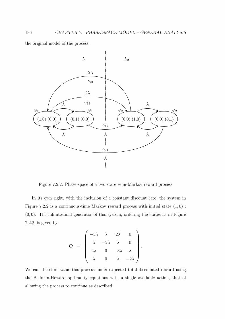
136 CHAPTER 7. PHASE-SPACE MODEL – GENERAL ANALYSIS
the original model of the process.
ϕ1 ϕ2
γ12
γ21
(1,0):(0,0) (0,1):(0,0) (0,0):(1,0) (0,0):(0,1)
ϕ1 ϕ2
λ
λ λ λ
λ
λ
L1 L2
2λ
γ12
2λ
γ21
Figure 7.2.2: Phase-space of a two state semi-Markov reward process
In its own right, with the inclusion of a constant discount rate, the system in
Figure 7.2.2 is a continuous-time Markov reward process with initial state (1, 0) :
(0, 0). The infinitesimal generator of this system, ordering the states as in Figure
7.2.2, is given by
Q =
−3λ λ 2λ 0
λ −2λ λ 0
2λ 0 −3λ λ
λ 0 λ −2λ
.
We can therefore value this process under expected total discounted reward using
the Bellman-Howard optimality equations with a single available action, that of
allowing the process to continue as described.

7.2. PHASE-SPACE CONSTRUCTION 137
Now consider the above reward process with the addition of a second action that
affects the rewards defined for the process in each state, along with the distribution
of time spent in each state. In effect, we now have a semi-Markov decision process
where the holding time of each state is dependent on the action selected upon hitting
that state. Under selection of the first action, the duration of time spent in each of
the states is of PH -type with representation (α,T ) as given above. Suppose that
under selection of the second action, the holding time in each state is distributed
according to a PH -type distribution with representation (ω,U ).
From an SMDP perspective, the currently selected action defines the dynamics
of the process. In other words, we know which of the phase transition structures, T
or U in our example, apply to the phase-space of the model via the current action
selection. As such, at any given time we only require knowledge of the current
action and hence the transition structure of a single holding time distribution. In
our model, we require a single phase-space that is consistent with any possible action
selection in each of the states of the original system. One possible construction is to
create a separate phase-state structure for each of the PH generators corresponding
to the actions that may be selected in each state. Then, the overall phase-state
structure can be given by the Cartesian product of these separate structures. This
construction, however, increases the size of the phase-space unnecessarily. Once an
action is selected we do not require knowledge of the phase transition structures of
any holding time distribution other than that corresponding to the current action.
Therefore, we just need a simple phase-space for each state that can determine the
holding time distribution given the current action selection.
Note that the order of the PH -generator matrices T and U may differ. From
a Bellman-Howard perspective, we require the infinitesimal generator matrices for
the entire process for each possible action to be of the same dimension. To accom-
plish this, we may simply add rows and columns of zeros to the end of all smaller
PH -generator matrices to pad them out to the size of the largest for each of the
states and similarly add zeros to the end of all corresponding initial state vectors.
With regard to reward received in a given level of the phase-space, we allocate no

138 CHAPTER 7. PHASE-SPACE MODEL – GENERAL ANALYSIS
permanence reward to those phase-states that are added for dimensionality purposes
in the representation of the holding time distributions.
A much more subtle issue involves the initial state vectors α and ω. We have
already dealt with differing dimension by padding the smaller with zeros, so suppose
that α and ω are the same size. With a little thought we find that the initial vectors
must in fact be equal ; that is, the initial phase distribution of a holding time must
be the same for all possible action selections in every state. The reasoning behind
this restriction lies in the use of PH distributions and what this means for the
phase-space of our model.
Consider the phase-space of our small example given in Figure 7.2.2. The transi-
tions corresponding to leaving level 1 are equivalent to those entering level 2. Upon
entering level 2, we have effectively defined the initial distribution of the holding
time of level 2 by the phase-state occupancy in our phase-space model, and yet we
have not yet selected an action in that level. From a modelling perspective, we
cannot then choose an action such that the initial state vector of the holding time
distribution in level 2 contradicts the actual phase-state occupancy. Alternatively,
we cannot allow the decision made in level 2 to affect the transition out of level
1, as this would require pre-visibility of that decision. Therefore, the initial phase
distribution of all possible PH holding times in a given state under action selec-
tion must be independent of action selection. Although this requirement may seem
overly restrictive, we can limit our individual PH approximations or permissible PH
distributions to the class of PH distributions with initial phase distribution given
by (1, 0, . . . , 0), to which the very versatile Coxian distributions belong. As we have
previously mentioned, much work has been done on the fitting of statistical data
to Coxian distributions such as in Faddy [29] and Osogami and Horchol-Balter [70],
and so the unique initial phase distribution issue may be somewhat bypassed in this
manner.
Another aspect to consider, which is not present in the above example, is that of
competing distributions. Once an action is selected in a state, it may be possible to
transition to one of multiple other states, where the actual transition occurs when
7.2. PHASE-SPACE CONSTRUCTION 139
the first of the concurrent holding times expires. The first of the PH holding time
distributions to expire, being the minimum of the competing distributions, is also
of phase-type, as per Theorem 2.2.9 of Neuts [66]. This minimum distribution is
therefore the holding time distribution in the state of interest and an infinitesimal
generator for the phase-space of the process may be constructed by repeating this
concept for all states, making sure that the previous two issues of dimension and
initial phase distributions are addressed. In general, the representation of such
a minimum distribution requires one or more Kronecker products to allow for all
possible combinations of phase occupancies of the competing distributions. An
example of this type of construction is given in Neuts and Meier [67] from a reliability
modelling perspective. In general, however, there may be more than two competing
distributions and one must pay careful attention to the resulting transitions relating
to which of the distributions expires first. The construction of a phase-space is
therefore extremely system dependent and, in certain situations, as in the earlier
Erlang race, it may be possible to simplify the phase-space if it is not important
which of the competing distributions expires first.
We mention at this point that the various aspects and restrictions discussed
above relate to the modelling of a physical system and so are necessary for accurate
representation. From a mathematical viewpoint, all that is required for the solution
of the MDP formed on the phase-space of the system is a reward structure and
infinitesimal generators for each of the possible actions. In other words, the solution
techniques of general MDPs can handle far more general systems than those on which
we are focusing. Recall, however, that we are utilizing the PH representations, or
approximations, to form an MDP as the original system can be too complex to solve
directly. In these situations, we must be cautious in the modelling and construction
of the phase-space and resulting generator matrices. While the construction itself is
not overly difficult, it is certainly not trivial in general and yet received very little
treatment in Younes and Simmons [96] and Younes [95].
Once we have formed the transition matrices for the phase-space of the system
and defined an appropriate reward structure, with the inclusion of a constant dis-

140 CHAPTER 7. PHASE-SPACE MODEL – GENERAL ANALYSIS
count factor, we have a standard MDP. We can therefore solve this decision process
using the Bellman-Howard optimality equations. This technique, however, values
the phase-space process, which we note may not translate directly to the valuation
of the original model. We must be careful when comparing valuations, and policies
for decision processes, of the two systems with respect to the information available
to the decision maker in the original model. The neglect of this caution is where the
technique in Younes [95] fails, as was demonstrated in the previous chapter. In the
next section, we describe an action-consistent valuation technique, first introduced
in Section 6.3 for a specific case, to address this fundamental issue of our phase-space
technique.
7.3 Action-Consistent Valuation
The principle of optimality utilized in the solution to the Bellman-Howard optimality
equations means that the resulting solution provides an optimal policy for all states
of an MDP. The issue with the phase-space model is that the decision maker should
not have definite knowledge of phase-occupancy at all times. Phases are introduced
as a vessel for the solution of a decision process which would otherwise be too
complex. As such, direct solution of the Bellman-Howard optimality equations on
the phase-space of a system provides information to the decision maker that would
otherwise be unavailable in the original model. As the phase-space is a continuous-
time Markov chain, we can calculate probabilistic phase-occupancies via solution
of the Kolmogorov differential equations and condition on level occupancy where
appropriate as in Younes [95]. The issue of how to appropriately value the phase-
states to provide consistency between that of the phase-space model and the original
model is, however, unaddressed in the literature to date.
From the perspective of the decision maker, only the current level is visible
at any given time and not the actual phase-state occupied. We therefore define an
action-consistent (AC) valuation for the phase-states that replicates the information
available to the decision maker in the original model. First, let us consider the
7.3. ACTION-CONSISTENT VALUATION 141
solution of the phase-space decision process via direct use of the Bellman-Howard
optimality equations in order to illustrate the two primary issues regarding action
consistency within levels. This solution defines an optimal action for each of the
phase-states without any consideration for the level to which each of the phase-
states belongs. However, since we know that the decision maker should only be
making decisions based on level occupancy, we must modify the Bellman-Howard
optimality equations to take this concept into account.
The first issue we deal with is action consistency within the current level of
interest. Consider Li of the phase-space, comprised of phase-states i1, . . . , im. When
valuing a phase-state of Li, say for example i1, under a particular action a, our
AC valuation restricts the action taken in all of the other phase-states of Li to
be this same action, a. From the point of view of the decision maker, valuing the
state corresponding to Li of the original model under action a, there is no actual
knowledge of the exact phase-occupancy. Thus, by selecting action a in this state,
there is effectively a forcing of the selection of action a in every phase-state of Li
and hence our action-consistent valuation of the phase-space must also force this
particular outcome. This particular aspect of correct valuation is dealt with in
Younes’ technique, although it is not described in [95] as a necessary requirement.
The second and critical issue, neglected by Younes in [95], is that of enforcing an
action consistent view of all other levels from the perspective of the phase-states in
Li. The standard Bellman-Howard optimality equations operate on the phase-states,
yet we wish to reconstruct a level based policy. Therefore, we no longer wish to only
consider the probability densities of the first hitting times on all other phase-states
that are a single transition from our phase-state of interest, i1. Rather, we wish to
consider the probability densities of the first hitting times on all phase-states that
are a single level transition from our phase-state of interest. In the original model,
we would normally value the states utilizing the principle of optimality with one-step
state transitions, and this concept is the level-based phase-space equivalent. These
single level phase-state transitions can be easily represented by PH distributions,
where the phases are constructed from the structure of the phase-space and the

142 CHAPTER 7. PHASE-SPACE MODEL – GENERAL ANALYSIS
absorbing state of the distribution is that of the target level.
Consider a second level, Lj, which is reachable in a single level transition from
Li. The contribution to the value of phase-state i1 from phase-state j1, say, which
is reachable in a single transition from Li is the value of j1 discounted appropriately
according to the first hitting time of j1 from i1. The aspect that sets our AC
valuation apart from the existing techniques in the literature, such as the QMDP
technique [59], is how we value the phase-states of Lj in the valuation process.
In the POMDP literature, the phase-states of Lj are physical entities that are not
necessarily always visible and so the idea of valuation is to emulate the behaviour if
they were visible. In our situation, and also in Younes [95], the phase-states are not
part of the original model and so the behaviour we wish to replicate is that of the
decision maker in the original model who only has knowledge of level occupancy.
Younes however values the phase-states of the destination levels, Lj in our example,
via the QMDP valuation technique. This technique effectively allows each of the
phase-states to behave optimally and hence implies that the decision maker has
knowledge of which of the phases are occupied and the optimal action to take in
each case. The resulting valuation permits the decision maker to make different
action selections upon hitting a target level based on the phase-state in which it
arrives, which is clearly not a feature of the original model.
The decision maker in the original model may only make different action selec-
tions to achieve optimality based on the time at which a level is first occupied. This
means that at this hitting time, the action selected must apply in all phase-states, as
definitive knowledge of phase-state occupancy is not available. Therefore, returning
to our illustrative example, upon hitting Lj, the optimal action for the level at this
hitting time is applied in all phase-states of Lj and these phase-states are valued
accordingly. Noting that this action may not be optimal for all phase-states of Lj
individually, it nevertheless forces a consistent action to be taken at this hitting time
that is optimal on a level basis and hence our AC evaluation maintains the level
focus present in the original model.
Acknowledging that we are yet to discuss the logistics of initiating and performing

7.3. ACTION-CONSISTENT VALUATION 143
such a valuation, topics that we will cover in Sections 7.4 and 7.5, once we have
performed an AC valuation for all of the possible actions that may be selected in
the phase-states of a level, the optimal action is simply the action corresponding
to the highest value. If the optimal policy specifies the same optimal action for
all of the phase-states in a level, then we say that the level is action-consistent.
A direct result of this property is that when we construct a level based optimal
policy, the policy will be time-independent. Also, with regard to our AC valuation,
when considering arrival to an action-consistent level, the absolute time of arrival is
inconsequential to the valuation process, and we need only consider the time taken
to hit the level in order to apply appropriate discounting.
If we find that all of the levels in the phase-space system are action-consistent,
then all of the optimal policies for each level are time-independent. Note that
a standard MDP is a special case of a system where all of the levels are action-
consistent, since each level consists of a single phase-state in the phase-space model.
On the other hand, if we find that a level is not action-consistent, then we must take
care in the entire valuation process to maintain a level-based view of the system.
To summarize the AC valuation technique, there are two primary issues ad-
dressed that permit an accurate phase-state valuation from a level-based viewpoint:
1. When valuing a phase-state of a given level under a given action, that action
must also be selected in all other phase-states of the given level.
2. When considering the hitting time at a given level under optimality, the ap-
propriate level-based optimal action applicable at that hitting time must be
applied in all phase-states of the level.
The first point has been largely addressed in the POMDP literature, but the
second is a new addition that is vital to the accuracy of our phase-space technique,
when compared to direct solution of the original model via the optimality equations
given in Section 4.4.
As in Section 6.3, where this valuation technique was first introduced, we use
the subscript AC on the phase-state values to denote the technique used. As such,

144 CHAPTER 7. PHASE-SPACE MODEL – GENERAL ANALYSIS
V abi,AC(s) indicates the value of phase-state bi when action a is selected at decision
epoch s utilizing our AC valuation technique. The value for a level, LB, when action
a is selected at time s is therefore given by
V aLB
(s) =∑
bi∈LB
P [bi occupied at s|LB occupied at s] V abi,AC(s).
The optimal behaviour in level B at time s is therefore determined by the action
that achieves the optimal value at s, where this value is given by
V ∗LB
(s) = maxa{V a
LB(s) }.
We use this expression for the optimal value to identify the absolute times of optimal
action changes, if any exist, for the level under consideration. These times then en-
able us to form action-consistent intervals in the valuation process when performing
calculations based on the hitting time on this level.
We note that, in practical application of the AC valuation technique, the re-
quirements above are somewhat cyclic. To value a phase-state, we must identify
the action-consistent intervals of the levels on which the phase-state directly de-
pends. However, to determine action-consistent intervals, we must have valued the
phase-states of the desired level. We will address this topic in Section 7.5, but nev-
ertheless the AC valuation technique is mathematically sound and so we proceed to
the statement of the unifying result of our phase-space technique.
7.4 Optimality Equations
Consider the general optimality equations given in equation (7.1.1). To simplify the
equations in the following discussion, we define a single reward term for state i at
time s under action a∗, ra∗
i (s), such that
ra∗
i (s) =∑
k∈S
∫ ∞
s
[(∫ θ
s
ϕa∗
i e−β(α−s)dα
)
+ γa∗
ik e−β(θ−s)
]
dP a∗
ik (s, θ), (7.4.1)
for all i ∈ S and s ≥ 0.

7.4. OPTIMALITY EQUATIONS 145
Therefore, we may re-write equation (7.1.1) using this notation as
V ∗i (s) = ra∗
i (s) +∑
k∈S
∫ ∞
s
V ∗k (θ)e−β(θ−s)dP a∗
ik (s, θ), ∀i ∈ S and s ≥ 0, (7.4.2)
where action a∗ is the optimal action to select in state i at epoch s. Once again, we
note that the optimal action may vary according to the absolute time of the decision
epoch; that is, the optimal policy may be time-dependent.
As the optimal action to select in state i at epoch s may vary, so too may the
optimal action in state k at the first hitting time at state k from state i, θ. We
can, however, break the interval [s,∞) for the possible hitting times at state k into
action-consistent intervals using the notation defined earlier. Recall that there are
Tk action-consistent intervals for the optimal policy for state k, with tk(ℓ) the ℓth
absolute time of change of action and a∗k(ℓ) the optimal action in the ℓth interval.
Define
uk(ℓ) = max{ s , tk(ℓ) }
for all k ∈ S, s ≥ 0 and ℓ = 0, . . . , Tk. An equivalent system of equations to those
in (7.4.2), incorporating action-consistent intervals, is therefore given by
V ∗i (s) = ra∗
i (s) +∑
k∈S
Tk∑
ℓ=1
∫ uk(ℓ)
uk(ℓ−1)
Va∗
k(ℓ)
k (θ)e−β(θ−s)dP a∗
ik (s, θ),
∀i ∈ S and s ≥ 0. (7.4.3)
Note that, in the above equation, we can specify the optimal action to take in state
k at the hitting time θ, as we are operating within an interval where the optimal
action is constant over the entire interval.
Now let us consider the phase-space of this model. To differentiate in notation
between phase-states and states, we denote level i, Li, to be the collection of phase-
states corresponding to state i. With regard to the phase-states themselves, we
attach a subscript to the state notation, and so im ∈ Li indicates the mth phase-
state belonging to level i. When valuing state i at epoch s, the system must be in
one of the phase-states of Li. Although the decision maker does not know exactly
146 CHAPTER 7. PHASE-SPACE MODEL – GENERAL ANALYSIS
which phase-state is occupied at epoch s in general, the calculation of the probability
that a particular phase-state is occupied, given the level occupancy, is a relatively
straightforward task. As the phase-space is a continuous-time Markov chain, given
the action selected in Li which governs the phase-state transition dynamics of Li,
we may calculate P [im occupied at s|Li occupied at s] at any decision epoch s via
the Kolmogorov differential equations. Here, we firstly calculate the probability
of being in each of the phase-states of Li individually at s, given an appropriate
initial phase-state or phase-state distribution for the system, and then condition
accordingly on being in Li at s. Shortening the notation to Ps[im|Li], and similarly
P [im occupied at s] to Ps[im], we have that
Ps[im|Li] =Ps[im]∑
ij∈Li
Ps[ij]
for all im ∈ Li and s ≥ 0.
Similarly, upon first arriving to state k, the system must arrive into one of the
phase states kn of Lk. Consider the probability density of the first hitting time at
phase-state kn, given that the process is in phase-state im at decision epoch s and
action a∗ is selected, dP a∗
imkn(s, θ). The path of phase-states that are traversed in
a transition from im to kn form a Markov chain where all the phase-states belong
to Li except for the destination phase-state kn. If we think of phase-state kn as
an absorbing state, then this density may be described as a PH distribution. The
generator matrix is defined by the transition rates amongst phase-states of Li when
the appropriate level-based optimal action, a∗, is applied in all phase-states im ∈ Li.
Once an action is chosen at time s in any phase-state of Li, the next decision epoch
in the original model is not until we have left this level. Therefore, on selecting an
action in any of the phase-states, we must then also select this action in all other
phase-states of Li. Importantly, this optimal action is therefore applied in all phase-
states and thus a level-based action-consistent view of the process is maintained.
Given the hitting time, θ, on phase-state kn, we need to appropriately discount
the value of kn. Equation (7.4.3) divided the possible hitting times into action
consistent intervals. Therefore, on hitting Lk in one of these intervals, we know the
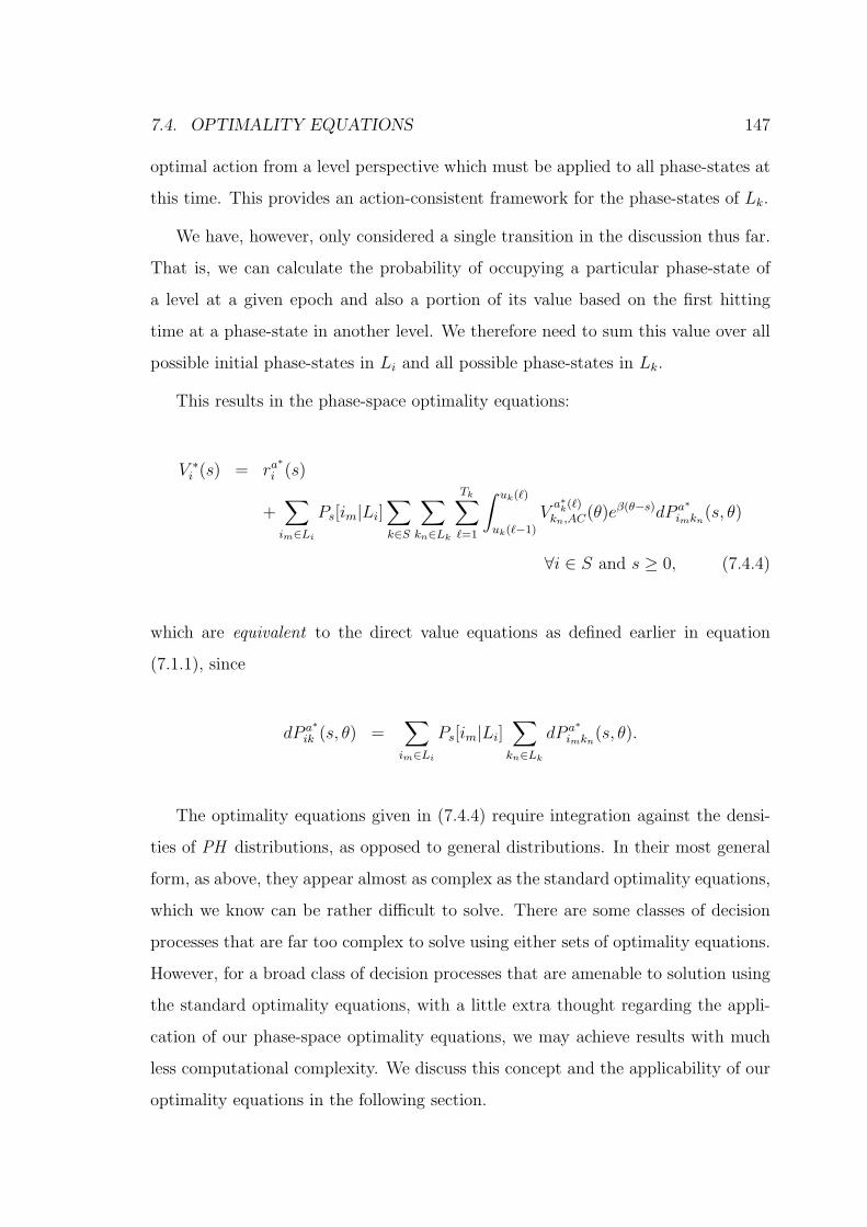
7.4. OPTIMALITY EQUATIONS 147
optimal action from a level perspective which must be applied to all phase-states at
this time. This provides an action-consistent framework for the phase-states of Lk.
We have, however, only considered a single transition in the discussion thus far.
That is, we can calculate the probability of occupying a particular phase-state of
a level at a given epoch and also a portion of its value based on the first hitting
time at a phase-state in another level. We therefore need to sum this value over all
possible initial phase-states in Li and all possible phase-states in Lk.
This results in the phase-space optimality equations:
V ∗i (s) = ra∗
i (s)
+∑
im∈Li
Ps[im|Li]∑
k∈S
∑
kn∈Lk
Tk∑
ℓ=1
∫ uk(ℓ)
uk(ℓ−1)
Va∗
k(ℓ)
kn,AC(θ)eβ(θ−s)dP a∗
imkn(s, θ)
∀i ∈ S and s ≥ 0, (7.4.4)
which are equivalent to the direct value equations as defined earlier in equation
(7.1.1), since
dP a∗
ik (s, θ) =∑
im∈Li
Ps[im|Li]∑
kn∈Lk
dP a∗
imkn(s, θ).
The optimality equations given in (7.4.4) require integration against the densi-
ties of PH distributions, as opposed to general distributions. In their most general
form, as above, they appear almost as complex as the standard optimality equations,
which we know can be rather difficult to solve. There are some classes of decision
processes that are far too complex to solve using either sets of optimality equations.
However, for a broad class of decision processes that are amenable to solution using
the standard optimality equations, with a little extra thought regarding the appli-
cation of our phase-space optimality equations, we may achieve results with much
less computational complexity. We discuss this concept and the applicability of our
optimality equations in the following section.

148 CHAPTER 7. PHASE-SPACE MODEL – GENERAL ANALYSIS
7.5 Level-skipping in the Phase-Space
We have defined a new set of optimality equations for the phase-space model; how-
ever, they can be potentially as complex to solve as the original optimality equations.
This is due to the fact that, although we have simplified the representation of the
level to level transitions by exploiting PH distributions, we are still dealing with
a system of Volterra equations of the second kind. These nested integrals are ex-
tremely difficult to solve when the state-space contains cycles due to the lack of an
obvious starting point of solution. This of course does not mean that a solution does
not exist, but that if one exists, it would not be easy to find. There are numerical
algorithms for handling the solution of a single Volterra equation of the second kind,
such as Garey [33] and Bellen et al. [11]. Nevertheless, to the author’s knowledge,
there are no algorithms for systems of these equations and so we avoid the analysis
of processes that result in such optimality equations.
To avoid the cyclic nesting of the value functions in the optimality equations, we
henceforth restrict our discussion to processes on acyclic state-spaces. When valu-
ing processes with acyclic state-spaces, if the number of states is finite as we have
assumed throughout this thesis, then there must be one or more absorbing states.
In other words, the process must eventually end in one of these absorbing states. It
is these end states that enable us to solve the optimality equations via the backward
recursion principle of dynamic programming. Both the original optimality equations
and the phase-space equations benefit from the lack of cycles in the state-space with
regard to their respective solution. We note, however, that even with this struc-
tural nicety, the original optimality equations may still be rather computationally
complex, as demonstrated in Chapter 5.
Our phase-space optimality equations are certainly not immune to complexity
issues and, for some systems, the difficulty in finding a solution is directly comparable
to that of the original optimality equations. There are nevertheless scenarios that
can arise in the phase-space model that enable us to exploit properties of Markov
chains and PH distributions in order to achieve results with much less computational

7.5. LEVEL-SKIPPING IN THE PHASE-SPACE 149
effort. We therefore proceed to define some identifying level characteristics that will
aid in this exploitation.
In the phase-space model, each phase-state has its own optimal value function
when the optimal action is selected in that phase-state. From equation (7.4.4), such a
value function is given by Va∗
k(ℓ)
kn,AC(θ) which denotes the value of phase-state kn ∈ Lk
at the hitting time θ of kn when the appropriate optimal action for the hitting
time, a∗k(ℓ), is selected. Note that it is possible for the optimal value functions
of the phase-states to be dependent on the absolute time at which they are first
entered. However, it is also possible for these value functions to be independent of
the absolute time of valuation. Therefore, for those phase-states that have time-
independent optimal values, their contribution to the optimality equations can be
greatly simplified. By taking the constant phase-state value outside of the integral
in equation (7.4.4), the remaining integral involves only a single matrix exponential.
This integral calculates the expected discounting over the duration of the waiting
time until the arrival at the destination phase-state of interest. Examples of the
simple nature of these calculations can be found in Section 6.3.3.
The time-dependent, or independent, nature of the phase-state value functions
has the potential to greatly simplify the optimality equations. In order to identify
where we may be able to utilize such simplifications, we define a time-dependence
property on a level-based framework. We say that a level is time-independent (TI)
if all of its constituent phase-states have time-independent optimal value functions.
If a level is not time-independent, then we say it is time-dependent (TD). At this
point we stress that the time-dependence property, TI or TD, of a level in the
phase-space is a different concept from that of the time-dependence of the optimal
value function for the level itself. As an example, a TI level can, through the
probabilistic weighting based on the likelihood of phase-state occupancy, give rise
to a time-dependent optimal value. When valuing the phase-space, however, we are
predominantly concerned with values from a phase-state perspective. As such, we
focus on the time-dependence properties of the phase-states rather than the levels
themselves.

150 CHAPTER 7. PHASE-SPACE MODEL – GENERAL ANALYSIS
We define another level property with respect to the optimal policy, that of
action consistency, as defined earlier in Section 7.1. An action-consistent (AC) level
in the phase-space is a level such that the optimal action is the same for all possible
decision epochs. In other words, an AC level has a single action-consistent interval.
Any level that consists of two or more action-consistent intervals is said to be non
action-consistent (NAC).
The level properties that we have just defined are not necessarily directly related,
and, in fact, we have already seen examples of (TI,AC), (TI,NAC) and (TD,AC)
levels in our examples in Chapter 6. The fourth combination, (TD,NAC), is also
theoretically possible, but it did not appear in our earlier examples. All levels
in the phase-space therefore fall into one of these four categories and, as we will
demonstrate, we can simplify the phase-space optimality equations by preferring to
focus on certain categories and level-skipping if appropriate.
The phase-space value equations we have defined follow the convention of valuing
a level with respect to all immediate neighbouring levels. Suppose we wish to value
a level via an already valued direct neighbour that is a TD level, indicating that
we cannot simplify the optimality equations. Suppose also, however, that a direct
neighbour of our valued level happens to be a TI level. Depending on the action-
consistency property of the intermediate TD level and the TI level, we may be
able to skip over the TD level in the valuation process. This would enable us to
simplify the optimality equations and solve for optimality of our level of interest with
far less computational complexity than that of the original optimality equations.
Figures 7.5.1 and 7.5.2 show examples of skipping a TD level that is NAC and AC
respectively, for a system with a sequential state-space as in the race.
Note that, in the Figures 7.5.1 and 7.5.2, we have omitted the action-consistency
property of the valued TI level as it is inconsequential to our technique. The im-
portant factor is that it is TI, and action-consistency only comes to the forefront
when determining whether or not level-skipping of a TD level is appropriate.
Firstly, consider the example shown in Figure 7.5.1 where level 2 is TD and NAC.
When valuing level 1, the natural approach from a dynamic programming viewpoint

7.5. LEVEL-SKIPPING IN THE PHASE-SPACE 151
L1
L2
(TD, NAC)
L3
(TI)
PH
General
Figure 7.5.1: Level-skipping of a (TD,NAC) level
L1
L2
(TD, AC)
L3
(TI)
PH
PH
Figure 7.5.2: Level-skipping of a (TD,AC) level
152 CHAPTER 7. PHASE-SPACE MODEL – GENERAL ANALYSIS
is to consider the hitting time at level 2, which in our phase-space construction is
given by a PH distribution. As the phase-state values of level 2 are time-dependent,
we cannot simplify the phase-space optimality equations any further than those
given in equations (7.4.4). Looking past level 2 to level 3, it is possible to focus
on the hitting time at level 3 from level 1, bypassing any calculations involving the
time-dependent phase-state values of level 2. The hitting time at level 3, however,
is dependent on the transition properties of level 2 and so we must be very careful
in formulating its distribution, which may not be PH.
Action selection in general has a bearing on either the transition probabilities,
the reward structure, or both, in the original model. Translating this to the phase-
space model, constructing the PH hitting time at level 3 requires knowledge of the
behaviour of the process in the phase-states of level 2. Since level 2 is NAC, we
require knowledge of the hitting time at level 2 in order to know which action-
consistent region is applicable and hence which action is invoked in level 2 at that
time. Due to the dependence on the absolute time of action change, we no longer
have a PH distribution and thus lose the ability to exploit phase-space properties in
a simple manner. If the different action-consistent regions happen to give rise to the
same phase-space transition matrix passing through level 2, then the different action
selection must affect the reward structure for the actions to be distinct from one
another. In this situation, while the hitting time distribution can now be represented
as a regular PH distribution, the reward simplification of equation (7.4.1) is invalid.
Again, the actual hitting time of level 2 is required to calculate when the reward
structure changes due to the different action-consistent intervals. In essence, we
have a simple PH transition structure, but a complicated reward structure such
that it serves little purpose to implement level-skipping.
Complicating matters further, if we wish to skip multiple (TD,NAC) levels,
then the decision maker requires knowledge of each of the hitting times at each of
the intermediate (TD,NAC) levels in order to accurately model the situation. In
particular, if the transition probabilities are dependent on action selection, then the
construction of the hitting time distribution at the target TI level can be extremely
7.5. LEVEL-SKIPPING IN THE PHASE-SPACE 153
complex. It requires dividing each hitting time at the target level into regions
for all possible combinations of action-consistent intervals that can occur in the
intermediate (TD,NAC) levels along the way. It is therefore not recommended to
attempt to level-skip any (TD,NAC) levels, as the alternative of direct calculation
involving time-dependent phase-state values using equations (7.4.4) is certainly no
more complex than level skipping and is a far more natural concept.
The idea of level-skipping does, however, have merit in certain situations and so
now we consider the example given in Figure 7.5.2. Level 2 in Figure 7.5.2 is TD
and AC. The fact that it is AC means that it has a single optimal action which is
selected at all times. As a consequence, when constructing the PH distribution for
the transition from level 1 to level 3, we need not keep track of the actual hitting
time of level 2. All that is necessary is that we construct the PH -generator matrix
for this transition while enforcing the appropriate action in the phase-states of level
2. The reward simplification given in equation (7.4.1) is invalid for level skipping
here also, but an alternative is easily calculated. Although the reward structure
of the intermediate level may be different from the starting level, we know exactly
what the structure is, and it is constant as the intermediate level is AC. Therefore,
we simply have a Markov reward process on the phase-space with respect to the
level transitions, as action selection is fixed, and can easily value the process using
the techniques outlined in Chapter 2.
Therefore, in order to avoid integrals involving time-dependent phase-state values
in the value equations, we may skip any number of (TD,AC) levels if they lie
between the current level under consideration and an already valued TI level. To do
so, we can easily construct a PH -generator matrix on the phase-space representing
this transition and a simplified reward component by valuing the Markov reward
process formed by this generator matrix. The complexity of the integrals for TD
levels are absorbed into the PH distribution for transitions over multiple levels;
however, all this added complexity affects is the size of the generator matrix. Thus,
while levels that are (TD,NAC) are troublesome, we can truly take advantage of
the Markovian properties of the phase-space by level-skipping (TD,AC) levels in

154 CHAPTER 7. PHASE-SPACE MODEL – GENERAL ANALYSIS
our phase-space technique. Figure 7.5.3 shows an example of where the phase-space
technique of level-skipping can be applied on a more complicated state-space than
those considered thus far.
L1
L2
(TI)
L3
(TI)
L5
(TI)
L6
(TI)
L4
(TD,AC)
PH
PH
Figure 7.5.3: Example of level-skipping in the phase-space technique
As the states of the process in Figure 7.5.3 involve branching, when valuing
level 1, there must be a contributing component from each branch. Thus, we can
value level 1 using the contributions from the TI level 2 and, via level-skipping, the
TI level 5. In such a process, we can avoid all integrals involving time-dependent
phase-state values and hence simplify the phase-space optimality equations.
7.6 The Phase-Space Technique
Suppose we have an acyclic process and have constructed its corresponding phase-
space as per Section 7.2. Note that the resulting phase-space need not be acyclic, as
the PH distributions may be cyclic absorbing Markov chains. The acyclic restriction
on the original process stems from the requirement for a starting point for the
solution process from a level-based perspective. The Bellman-Howard optimality

7.6. THE PHASE-SPACE TECHNIQUE 155
equations permit cyclic state-spaces because the algorithmic solution techniques
search for a stationary solution. Once we allow time-dependent state-transitions,
we know from experience that time-dependent optimal solutions may result and
hence we no longer have a stationary solution. As such, in order to make headway
into this field of complex decision processes, we require acyclic state-spaces so that
we may define an efficient solution technique.
Given the phase-space model, we begin by solving for optimality in the phase-
states of the levels that do not depend on any others. We refer to these levels as
end levels. We can easily reconstruct a level-based optimal value and hence policy
using phase-occupancy probabilities and thus we have our starting point for the
phase-space technique. The technique then propagates these solutions back through
the state-space of the system; that is, on a level by level basis, toward the beginning
of the state-space as in the backwards recursion principle of dynamic programming.
We may solve for an optimal value function, and hence optimal policy, for each level
by obeying one of the following rules for the contribution of each already valued
level on which our current level under consideration is directly dependent:
1. If the valued level is (TI,AC), then its contribution is simplified in the phase-
space optimality equations and so we propagate its optimal value directly. We
have seen this scenario in our examples multiple times, most often when the
valued level corresponds to the all arrived state of the race.
2. If the valued level is (TI,NAC), then its contribution is simplified in the phase-
space optimality equations and so we propagate its optimal value directly. Here
we pay particular attention to the hitting time on the valued level for each
of its action-consistent intervals to ensure the appropriate optimal value is
propagated. As an illustration, this situation arises in our standard K = 3
Erlang race example when considering level 1 which is directly dependent on
the valued threshold, and hence NAC, level 2.
3. If the valued level is (TD,AC), then we may potentially simplify the opti-
mality equations by observing the already valued levels along the path, or

156 CHAPTER 7. PHASE-SPACE MODEL – GENERAL ANALYSIS
paths, toward the end states. If all possible paths lead to a TI level with
only (TD,AC) levels as intermediate stages, then we may focus on these TI
levels and propagate their values back to our level of consideration directly.
This is done by formulating a PH hitting time at each TI level utilizing the
phase-space and modifying the single reward in the optimality equations to
the valuation of the subsequent Markov reward process. This simplification is
possible in our standard Erlang race example when considering level 0. For the
given parameters of this system, level 1 is (TD,AC), but level 2 is (TI,NAC)
and we have seen that skipping level 1 results in simpler phase-space value
equations. If, on the other hand, we encounter a (TD,NAC) level in the
search for TI levels, then it is unlikely that any simplification will be possible
and we just deal with the complexity of the optimality equations relating to
the closest valued (TD,AC) level.
4. If the valued level is (TD,NAC), then it is unlikely that any simplification will
be possible and we just deal with the complexity of the optimality equations.
Having valued the phase-states of the level under consideration, we may therefore
construct its optimal value function and label it as either of the 4 possibilities. It
is now a valued level and we continue with the technique in this manner until all
levels have been valued optimally.
We note, however, that it is almost impossible to determine a priori the class
of processes for which the simplifications outlined in our phase-space technique will
be applicable. Nevertheless, as our phase-space value equations and the standard
optimality equations are identical, we do no worse in terms of complexity by utilizing
our phase-space technique and leave open the opportunity to simplify the solution
process if an appropriate situation arises. In these situations, we utilize Markovian
properties of PH distributions to simplify the optimality equations that require
solution, making such solutions far more analytically tractable.
Chapter 8
Time-Inhomogeneous MDPs
8.1 Introduction
As mentioned in Hopp, Bean and Smith [40], the appropriate models for many
applications such as equipment replacement and inventory control are Markovian but
not time-homogeneous. In other words, a different problem is effectively encountered
at each decision epoch. In discrete-time, any finite state time-inhomogeneous MDP
can be reformulated as a denumerable state homogeneous MDP [8]. This can be
done by relabeling states to include both state and time-step information in the new
formulation.
When analyzing processes in continuous-time, we have already seen that, to
avoid direct solution of the integral value equations, it is desirable to discretize the
process. For a time-homogeneous MDP, we could either discretize the process into
fixed intervals or uniformize the process, both of which are discussed in Section 2.2.5.
In the former, if the discretization interval is too large, the decision maker may not
be able to observe all state transitions as they occur. Regular uniformization does
not suffer this lack of visibility, but requires a time-homogeneous process. Van Dijk
[87] proposes a uniformization technique for time-inhomogeneous Markov chains, but
this technique requires a continuum of transition matrices. Moreover, this relates to
time-inhomogeneity of the transitions of the process, and thus, if the inhomogeneity
of the decision process relates to the valuation of the process, then to the author’s
157

158 CHAPTER 8. TIME-INHOMOGENEOUS MDPS
knowledge no such uniformization-based discretization technique exists.
In fact, there is very little in the literature pertaining to the solution of time-
inhomogeneous continuous-time Markov decision processes. Hopp, Bean and Smith
[40] developed a new optimality criterion for such decision processes due to the
failings of valuation based on the renewal theory used in standard techniques, but
in the discrete-time scenario. This criterion is based on the concept of a rolling
horizon, in that the infinite horizon process is truncated at each stage to a finite-
horizon problem where this forecast horizon has certain characteristics pertaining
to optimal behaviour in the original process. Hopp [39] developed two algorithmic
approaches for the determination of whether a given finite horizon is a suitable
forecast horizon; however, as in the earlier work, they are restricted to the discrete-
time domain. Alden and Smith [3] and White [92] provide analyses of the error of
these rolling horizon techniques. More recently, Telek, Horvath and Horvath [85]
developed a technique for analysis of time-inhomogeneous Markov reward processes
in continuous-time from a differential equation perspective, but do not delve into
the realm of decision making and optimal control.
Boyan and Littman [16, 17] provide a solution technique for processes they term
time-dependent MDPs. These processes are continuous-time MDPs where the state
transitions and reward structure is allowed to depend on the absolute time of the
process. State representation is modified and expanded to include absolute time and
so the newly formed system effectively models the original system as an undiscounted
continuous-time MDP, where the discounting is incorporated into the reward struc-
ture. While the claim is that their technique can find exact solutions, it can only do
so for a limited range of problems. The reward structure is restricted to being piece-
wise linear and the state transition distribution functions discrete. Even then, the
equations that require solution are merely versions of the integral value equations
implementing these simplifications.
In the following section, we will introduce an approximation technique for the
solution of a class of continuous-time MDPs with time-inhomogeneous components
such as transition rates, reward structures and discounting. The restriction for

8.2. TIME-INHOMOGENEOUS DISCOUNTING 159
this class of processes is that all transitions and the reward structure, including
discounting, be governed by a single global clock. As a result of this requirement,
the reward structure cannot involve any relative rewards such as those relative to
the time since a state was first entered, as this would require knowledge of a second
clock keeping track of the time in the current state. We have generally avoided such
reward structures throughout this thesis, however, as they complicate the integral
value equations substantially.
This restricted class of processes nevertheless permits time-inhomogeneous per-
manence and impulse rewards, provided that their absolute values at any time are
dependent on only the single global clock and, of course, the state occupied. This
is more general than any reward structure considered thus far in this thesis. The
values of the process over time must be discounted according to some global dis-
count function based on the single global clock. Exponential discounting falls into
this category; it just so happens that, up to now, we have been thinking of it as
relative discount from a present value perspective due to its memoryless properties.
As long as we are careful assigning present values to our process, we can in fact
implement any discounting function we desire, as long as it applies for all possible
action selections and is relative to the global clock. All things considered, while
the class of decision processes suitable for our technique is restricted via the single
clock requirement, it is still more general than the majority of processes for which
solution techniques are available elsewhere in the literature.
8.2 Time-Inhomogeneous Discounting
Although we have allowed for general discount in the value equations of Section 4.4,
we have only considered exponential discounting thus far in this thesis. Exponential
discounting is the continuous-time analogue of a constant discount factor apply-
ing over all intervals in a discrete-time value process. In other words, exponential
discounting is akin to a time-homogeneous discount factor and so we refer to its
use herein as time-homogeneous discounting. Along with having an important re-

160 CHAPTER 8. TIME-INHOMOGENEOUS MDPS
lationship with finance, exponential discounting is also fundamental to the solution
of infinite horizon continuous-time MDPs. The Bellman-Howard optimality equa-
tions for infinite horizon MDPs require homogeneous discounting in order to find
the fixed point optimal solution. In the absence of such regularity in the discounting
of the values of the process, current techniques are restricted to solving the value
equations of Section 4.4, which, as noted throughout this thesis, when possible, is a
rather complicated task.
Real world processes, however, may require time-inhomogeneous discounting to
accurately represent the system being modelled. As an example, consider the Mean
Opinion Score (MOS) of a Voice-Over-IP (VoIP) transmission as the end-to-end
delay of the voice packets is increased. Figure 8.2.1 illustrates the decay of the MOS
score using the E-model [44], with appropriate system parameter default values for
a PCM codec [45], as the end-to-end delay is increased from 0ms to 500ms. The
MOS of 3.1 is also highlighted in this figure, and the significance of this value will
be explained in the following discussion.
0 50 100 150 200 250 300 350 400 450 5000
0.5
1
1.5
2
2.5
3
3.5
4
4.5
5Mean Opinion Score
End−to−end delay (ms)
MO
S
Figure 8.2.1: MOS decay as end-to-end delay is increased
Modelling a system of delay where the values are determined by the resulting

8.2. TIME-INHOMOGENEOUS DISCOUNTING 161
proportional decrease in MOS score requires time-inhomogeneous discounting. Con-
sider an increase in the delay of 50ms, where clearly the absolute time of when this
additional delay occurs has a bearing on the reward received. From Figure 8.2.1,
if this delay occurs in the first 50ms of the travel time of the VoIP packet, then
effectively, from a quality point of view, the delay would go unnoticed and hence
there is no decrease in MOS and thus no discounting required. However, if this delay
occurs later in the process, at say 150ms, then the resulting proportional decrease
over the duration of the delay is 0.986. Later still in the process, if the delay occurs
at 350ms, then the proportional decrease in MOS is 0.948 and so, to model the
process, we cannot simply use exponential (homogeneous) discounting, which would
give the same proportional decrease over all 50ms duration delays.
The MOS, using the formula for the E-model, continues in a steadily decreasing
fashion for end-to-end delays beyond 500ms; however, we have chosen to end our plot
in Figure 8.2.1 at 500ms. For one-way delay values exceeding 500 ms, the results are
not fully validated from a quality of service perspective as stated in [46]. Interactive
conversation is affected by delays above 150ms and it is highly recommended that
delays of 400ms or more be avoided from a network planning viewpoint [46]. That
is, maintaining an interactive conversation with end-to-end delays of more than
400ms can be extremely difficult. At first glance, it may appear that the MOS
corresponding to a 400ms, 3.56, indicates a reasonable level of quality from an
audio perspective. This score is approximately 80% of the maximum achievable
for the system, however this comparison is rather misleading with regard to user
satisfaction. Annex B of [44] tells us that while any MOS over 4.34 relates to a
scenario of all users very satisfied, a MOS of 3.56 falls into the range of many users
dissatisfied. Any MOS below 3.1 indicates that nearly all users are dissatisfied and
so, if we are valuing our system based on such user satisfaction levels, we may
wish to penalize these larger delays further than indicated solely by the decrease in
MOS. Therefore, it is not difficult to envisage a system whereby the absolute reward
received is unaffected in some region of time, decreases in a subsequent region before
dropping away to effectively nothing beyond some absolute time-point.

162 CHAPTER 8. TIME-INHOMOGENEOUS MDPS
8.3 The Random Time Clock Technique
The technique we have developed for the solution of these time-inhomogeneous
MDPs with a single global clock draws on various ideas discussed throughout this
thesis. As a general outline of the technique, we first consider the underlying state-
space of the original system, which for now we assume to be a Markov chain. A dis-
cussion of an extension of the technique pertaining to time-inhomogeneous Markov
Chain state-spaces appears in Section 8.3.6. To keep track of the absolute time of
the process, we modify the process to incorporate time into the state-space. We do
not represent time as a continuum, as in Boyan and Littman [16, 17], but rather as
discrete time points. As such, the system formed by implementing this technique is
therefore only an approximation to the original continuous-time process. However,
as will be demonstrated, this approximation can produce very accurate results with
a far less complex solution process.
The key to this technique is that the length of the interval between two con-
secutive time points is not fixed but exponentially distributed. We can therefore
construct a continuous-time Markov chain representation of our original process.
By appropriately defining the reward structure for each available action of the de-
cision process in each state, we have an ordinary continuous-time MDP which we
solve using whichever technique we prefer and then translate the resulting solution
back to a solution for the original system.
In order to illustrate the concepts throughout this section, consider the 2 state
continuous-time Markov process as depicted in Figure 8.3.1.
Define the state-space of the system to be S. To construct a reward process of
particular interest to our random time clock (RTC) technique, for all i, j ∈ S we
define a time-inhomogeneous reward structure. Let ϕi(t) be the instantaneous rate
of reward in state i at time t and let γij(t) be the impulse reward received for a
transition from state i to state j at time t, where t ∈ R+ is the absolute time of the
process. Define D(t) to be the absolute discounting of the process applied at time t
relative to time 0.
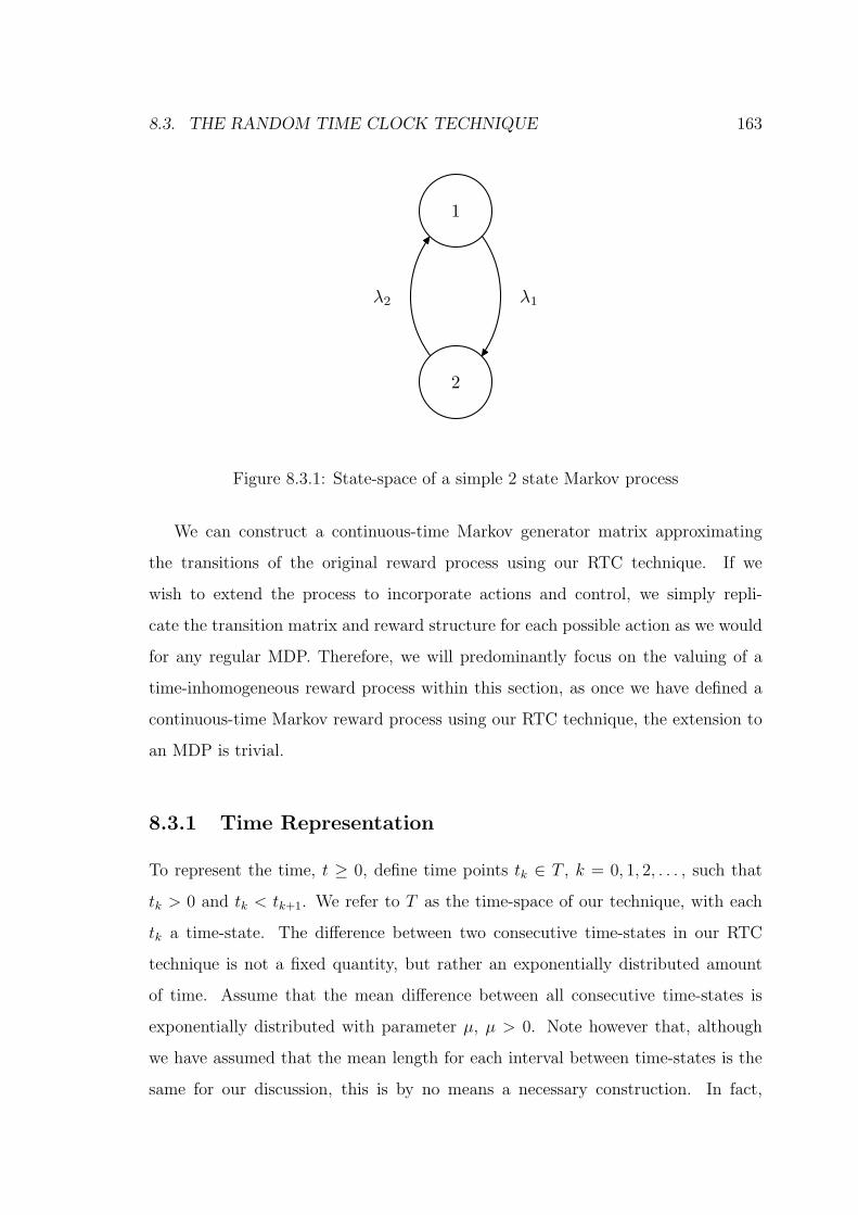
8.3. THE RANDOM TIME CLOCK TECHNIQUE 163
1
2
λ1λ2
Figure 8.3.1: State-space of a simple 2 state Markov process
We can construct a continuous-time Markov generator matrix approximating
the transitions of the original reward process using our RTC technique. If we
wish to extend the process to incorporate actions and control, we simply repli-
cate the transition matrix and reward structure for each possible action as we would
for any regular MDP. Therefore, we will predominantly focus on the valuing of a
time-inhomogeneous reward process within this section, as once we have defined a
continuous-time Markov reward process using our RTC technique, the extension to
an MDP is trivial.
8.3.1 Time Representation
To represent the time, t ≥ 0, define time points tk ∈ T , k = 0, 1, 2, . . . , such that
tk > 0 and tk < tk+1. We refer to T as the time-space of our technique, with each
tk a time-state. The difference between two consecutive time-states in our RTC
technique is not a fixed quantity, but rather an exponentially distributed amount
of time. Assume that the mean difference between all consecutive time-states is
exponentially distributed with parameter µ, µ > 0. Note however that, although
we have assumed that the mean length for each interval between time-states is the
same for our discussion, this is by no means a necessary construction. In fact,
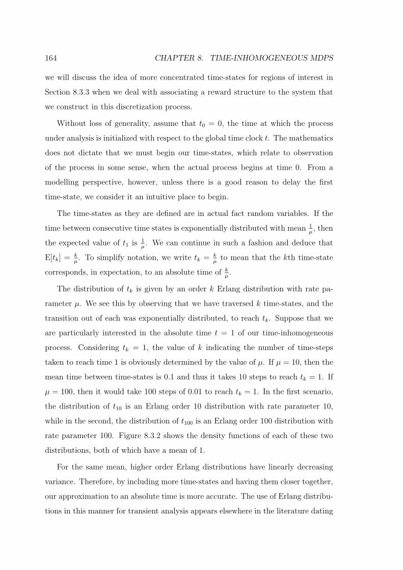
164 CHAPTER 8. TIME-INHOMOGENEOUS MDPS
we will discuss the idea of more concentrated time-states for regions of interest in
Section 8.3.3 when we deal with associating a reward structure to the system that
we construct in this discretization process.
Without loss of generality, assume that t0 = 0, the time at which the process
under analysis is initialized with respect to the global time clock t. The mathematics
does not dictate that we must begin our time-states, which relate to observation
of the process in some sense, when the actual process begins at time 0. From a
modelling perspective, however, unless there is a good reason to delay the first
time-state, we consider it an intuitive place to begin.
The time-states as they are defined are in actual fact random variables. If the
time between consecutive time states is exponentially distributed with mean 1µ, then
the expected value of t1 is 1µ. We can continue in such a fashion and deduce that
E[tk] = kµ. To simplify notation, we write tk = k
µto mean that the kth time-state
corresponds, in expectation, to an absolute time of kµ.
The distribution of tk is given by an order k Erlang distribution with rate pa-
rameter µ. We see this by observing that we have traversed k time-states, and the
transition out of each was exponentially distributed, to reach tk. Suppose that we
are particularly interested in the absolute time t = 1 of our time-inhomogeneous
process. Considering tk = 1, the value of k indicating the number of time-steps
taken to reach time 1 is obviously determined by the value of µ. If µ = 10, then the
mean time between time-states is 0.1 and thus it takes 10 steps to reach tk = 1. If
µ = 100, then it would take 100 steps of 0.01 to reach tk = 1. In the first scenario,
the distribution of t10 is an Erlang order 10 distribution with rate parameter 10,
while in the second, the distribution of t100 is an Erlang order 100 distribution with
rate parameter 100. Figure 8.3.2 shows the density functions of each of these two
distributions, both of which have a mean of 1.
For the same mean, higher order Erlang distributions have linearly decreasing
variance. Therefore, by including more time-states and having them closer together,
our approximation to an absolute time is more accurate. The use of Erlang distribu-
tions in this manner for transient analysis appears elsewhere in the literature dating

8.3. THE RANDOM TIME CLOCK TECHNIQUE 165
0 0.2 0.4 0.6 0.8 1 1.2 1.4 1.6 1.8 20
0.5
1
1.5
2
2.5
3
3.5
4
4.5Erlang density function with mean 1
x
f(x)
µ = 10, r = 10µ = 100, r = 100
Figure 8.3.2: Erlang density function of mean 1 with differing parameters
back to Ross [77]. Van Velthoven, Van Houdt and Blondia [89] utilize the phases of
Erlang distributions to approximate time epochs in their analysis of tree-like pro-
cesses. Asmussen, Avram and Usabel [4] and Stanford et al. [83] employed the
time to expiration of Erlang distributions to approximate fixed absolute boundaries
in their applications of interest. We will make use of this particular aspect when
discussing the accuracy of our technique with regard to valuation.
8.3.2 State-Space Construction
In a similar manner to that of Boyan and Littman [16, 17] and that mentioned in
Bean, Smith and Lasserre [8], we define a new state-space for our RTC model such
that absolute time is incorporated into the state-space. Let M be the state-space
of our technique such that M = S × T . The states, m ∈M , of our new state-space
are all the possible cartesian pairs of states of the original system and time-states.
We denote such states using the notation 〈i, tk〉 indicating state i and time-state
tk simultaneously occupied for all i ∈ S and tk ∈ T . This state-space construction

166 CHAPTER 8. TIME-INHOMOGENEOUS MDPS
differs from the aforementioned work in the literature as we are neither considering
time as a continuous entity ([16, 17]), nor are we working in the traditional sense of
discrete time with fixed intervals ([8]).
As the state-space, S, of the original model is a Markov chain, let Q = [qij] be
its infinitesimal generator matrix where qij is the rate of transition from state i to j
for all i, j ∈ S and i 6= j. Now consider a state m ∈M of our RTC state-space and
let m = 〈i, tk〉. Loosely speaking, we may think of this state, 〈i, tk〉, as state i of the
original model being occupied at time tk.
In this context, we allow two things to happen from this state. Suppose we
observe our newly formed process continuously. As an observer in continuous-time,
no two transitions can occur simultaneously. From state 〈i, tk〉, we could see a
transition from state i to some other state j ∈ S without a change in time-state.
On the other hand, our system may move to the next time-state, tk+1, and still be
occupying state i of the original model. As an intuitive description, we may think
of the knowledge of a time-state tk as taking a rough glance at the global time clock
to give us some idea of the current time of the process. We then return to observing
the dynamics of the system of the original model for an exponentially distributed
amount of time, until it is time to take another glance at the global clock to get a
new idea of the absolute time of the process.
As such, it is important to note that, when the state-space of the original model
is a Markov chain, the dynamics of our new state-space with respect to the state
transitions of the original model are precise. In other words, all real transitions of
the original model are seen in the transitions of our constructed state-space. We use
the time representation as an approximation to the global time in order to estimate
appropriate values for the time-inhomogeneous components of the original model,
such as the reward structure.
Therefore, as all transitions in our RTC system are exponentially distributed,
we may write down an infinitesimal generator for this process. Define Q = [qmn] to
be the generator of the RTC process where qmn is the rate of transition from state
m to state n for all m,n ∈ M and m 6= n. Let m = 〈i, tk〉 and n = 〈j, tℓ〉. The

8.3. THE RANDOM TIME CLOCK TECHNIQUE 167
transition rates for this system are given by
qmn =
qij, if j 6= i, tℓ = tk,
µ, if j = i, tℓ = tk+1,
0, otherwise,
(8.3.1)
for all m,n ∈M and m 6= n, with
qmm = −∑
n6=m
qmn. (8.3.2)
Figure 8.3.3 shows the RTC Markov chain state-space, M , of the process depicted
earlier in Figure 8.3.1.
〈1, 0〉
〈2, 0〉
λ1λ2
〈1, 1
µ〉
〈2, 1
µ〉
λ1λ2
〈1, 2
µ〉
〈2, 2
µ〉
λ1λ2
µ µ
µ µ µ
µ
t0 t1 t2
exp( 1
µ) exp( 1
µ) exp( 1
µ)
Figure 8.3.3: RTC State-space of a 2 state Markov process
The states in Figure 8.3.3 have been grouped according to the time-state pa-
rameter of the state notation by dashed rectangles. That is, the states in the first
rectangle correspond to state transitions of the original model while the system is
occupying time-state t0, the second for t1 and so forth. Note that, although there are
two transitions that relate to a time-state transition, the time taken for a transition
168 CHAPTER 8. TIME-INHOMOGENEOUS MDPS
from rectangle to rectangle is still governed by a simple exponential distribution.
This can be justified from a PH distribution perspective. Consider the states of one
rectangle to be the phases of a PH distribution and the next rectangle to be the
absorbing phase. The rate of absorption from every phase is the same, and so the
net result is that absorption occurs according to an exponential distribution, a result
shown in Section 2.1.1 of Bean and Green [9]. This result applies to any number of
phases and so the retention of exponential transitions between time-states, as shown
at the bottom of Figure 8.3.3, is valid for any Markov chain state-space, S, of the
original model.
Note that in this approximation technique, an observer of the process still sees
every state transition of the original model. There are no missed transitions as
there are if we were to discretize time into fixed intervals. An observer therefore
knows at all times which of the states of the original model is occupied; however,
the appropriate reward structure at that time must be approximated, which we will
now discuss.
8.3.3 Reward Structure and Discounting
Although we have approximated time in a discrete representation to incorporate it
into the state-space, we still observe the process in continuous-time. The built-in
time information is used to determine the appropriate reward structure for the state
under consideration. With a time-inhomogeneous reward structure, we may think of
the time-state information as a rough guide of the absolute time of the process. With
this discretized knowledge, we may construct a reward structure at various levels of
accuracy, depending on a number of factors, including simplicity of implementation.
Recall the time-inhomogeneous reward structure as defined for Figure 8.3.1. Fo-
cusing on state m = 〈i, tk〉 ∈ M , let us first consider the permanence reward appli-
cable for remaining in state i ∈ S. As was done in the analysis of continuous-time
MDPs in Section 2.3.4, we endeavour to replace the permanence reward with an
equivalent impulse reward. The only available knowledge regarding the absolute
time of the process, and hence the current value of the permanence reward ϕi(t),

8.3. THE RANDOM TIME CLOCK TECHNIQUE 169
is given by tk; that is, we expect the absolute time to be tk. Therefore, without
any further information available, effectively we have a constant permanence reward
applying over the entire duration of time spent in m, ϕi(tk).
As tk is in fact a random variable, we may choose how to interpret the quantity
ϕi(tk). Define dE(µ, k)(t) to be the density function of an order k Erlang distribution
with rate parameter µ for t ≥ 0. In other words, dE(µ, k)(t) is the density of
the distribution of tk. From a mathematical perspective, treating tk as a random
variable, we define
ϕi(tk) =
∫ ∞
0
ϕi(θ)dE(µ, k)(θ),
which gives the expected permanence reward at tk.
While the above definition is correct from a mathematical point of view, we can
opt for a simpler definition. We could make use of the expected value of tk and
define
ϕi(tk) = ϕi(tk), (8.3.3)
which is the permanence reward at the expected value of tk. These two alternative
definitions both have merit and so it is essentially a matter of personal choice, when
implementing the RTC technique, regarding which is more suitable.
Given the constant permanence reward, ϕi(tk), for remaining in state 〈i, tk〉,we must now determine an appropriate discount for the duration until the next
transition. Once again, the only knowledge of the current time of the process is that
time-state tk is occupied. Therefore, we assume a constant discount factor D(tk)
that applies the entire time that time-state tk is occupied, in a similar manner to our
treatment of the permanence reward. Note that we use the absolute discount from
the beginning of the process and build it into our reward structure. We will elaborate
on the reasons behind this in Section 8.3.5 when we discuss the implementation of
the RTC technique.
As for the permanence reward, we have a choice as to how we define the constant
absolute discount factor, D(tk). We can either use the expected absolute discount in

170 CHAPTER 8. TIME-INHOMOGENEOUS MDPS
state tk or the absolute discount at the expected value of tk. We leave the decision
as to which is more preferable to the reader.
Now that we have defined an appropriate permanence and discounting structure
for our expanded state-space M , we can formulate an equivalent impulse reward
for the duration of time spent in state m = 〈i, tk〉 before a transition. The rate of
transition out of state m is given by qm = −qmm. Let rϕm be the impulse reward
equivalent to the permanence reward received while occupying state m. Similar to
equation (2.3.4), as we are dealing with a single state within a Markov process, we
have that
rϕm =
∫ ∞
0
ϕi(tk)
(∫ θ
0
D(tk)dτ
)
qme−qmθdθ,
=
∫ ∞
0
(∫ θ
0
dτ
)
qme−qmθdθ ϕi(tk)D(tk),
=
(
1
qm
)
ϕi(tk)D(tk), (8.3.4)
for all m ∈M .
Consider the time-inhomogeneous impulse reward, γij(t) for a transition from
state i to state j at time t in the original model of the process. For a transition from
state m to another state n in our RTC state-space, we require an appropriate impulse
reward. With m = 〈i, tk〉, an impulse reward should be received on transition to
n = 〈j, tk〉 for i 6= j whereas earlier, the only information we have about absolute
time is built into the state-space. Therefore, we define γij(tk) to be the constant
impulse reward received on transition from m to n, m,n ∈ M . As usual, we have
our choice of interpretation of γij(tk); but, irrespective of our choice, the important
factor is that the impulse reward is constant.
As for the permanence reward, we must apply the appropriate discounting rel-
evant to the expected time we believe the process has been active. Define the
discounted impulse reward as
rγm,n = γij(tk)D(tk) (8.3.5)
for all m = 〈i, tk〉, n = 〈j, tk〉 such that i 6= j.

8.3. THE RANDOM TIME CLOCK TECHNIQUE 171
Using equations (8.3.4) and (8.3.5), we may now define a constant, impulse only,
reward structure for our RTC state-space M . Let m = 〈i, tk〉 and n = 〈j, tℓ〉. We
have an impulse reward rmn that takes into account the dynamics of the system,
given by
rmn =
rγmn + rϕ
m, if j 6= i, tℓ = tk,
rϕm, if j = i, tℓ = tk+1,
0, otherwise,
(8.3.6)
for all m,n ∈M .
The transition rates for our RTC state-space defined in equations (8.3.1) and
(8.3.2) define a continuous-time Markov process. With the inclusion of the reward
structure defined in equations (8.3.6), the resulting process is a time-homogeneous
continuous-time MRP. We have essentially absorbed all time-inhomogeneity result-
ing from the reward structure of the original model into the state-space of our RTC
technique.
8.3.4 Truncation
In Section 8.3.1, we spoke of the representation of time by constructing a time-space
T , consisting of exponentially spaced time-points. This enabled us to build time
information into the state-space and form a state-space that is a continuous-time
Markov chain. If the processes that we are modelling, however, are those with
an infinite planning horizon, then T contains a countably infinite number of time-
states. Thus the resulting transition matrix of our RTC state-space is an infinite-
dimensional matrix. From a practical perspective, if we wish to value the newly
constructed process, it may be necessary to truncate the sequence of time-states at
some point, tH , say.
The decision on the absolute time, tH , at which we truncate the process, is part of
the modelling of the process and will in general vary from application to application.
Including the spacing of the time-states, these properties of the time-space affect the
accuracy of the RTC technique, and it may take a few attempts at implementation
of the technique to achieve a desired outcome.

172 CHAPTER 8. TIME-INHOMOGENEOUS MDPS
Having decided on a final time-state, tH , we must then decide how to value the
RTC states corresponding to this time state, as well as how to model transitions at
this introduced finite-horizon. Exactly what is done in the truncation process can
be highly dependent on the properties of the time-inhomogeneous components of
the original model. The number of possibilities here is quite large and so we cannot
define a rule for every combination. We will, however, offer suggestions, regarding
certain properties in the original model, that will reduce the loss of accuracy in the
truncation of the process.
A naive but valid truncation method is to make tH as large as possible, such that
the dimension of the resulting RTC Markov process is still amenable to solution in
a reasonable amount of time. This method truncates our original infinite-horizon
model to a finite-horizon model by simply discarding all system information and
dynamics beyond the truncation time tH . In this scenario, we allow transitions
between the RTC states corresponding to the truncation time as defined by the
original model at this absolute time, and value the states as we would any other in
the process.
We can nevertheless look for certain properties of the original model and exploit
them if present. Suppose that we can find a truncation horizon tH , such that there
exists constants cϕiand cγi
for all i ∈ S such that for all t > tH ,
|ϕi(t)− cϕi| < ǫϕi
(8.3.7)
and
|γi(t)− cγi| < ǫγi
(8.3.8)
for ǫϕiand ǫγi
sufficiently small. In other words, for all t > th, the permanence and
impulse rewards for each state are close to constant in the original model, where the
closeness is defined by our choice of ǫϕiand ǫγi
. Suppose also that for this truncation
horizon tH , there exists a constant β such that for all t > tH ,
|D(t)−D(tH)e−β(t−tH)|D(t)
< ǫD (8.3.9)

8.3. THE RANDOM TIME CLOCK TECHNIQUE 173
for ǫD sufficiently small. This inequality is a requirement that the relative error
between the discount function and an exponential discounting function, initialized at
the horizon, is less than some defined parameter ǫD. If inequality (8.3.9) is satisfied,
the global discounting function is close to an exponential discount function with
parameter β once we are past the truncation horizon.
Therefore, if we can find a suitable truncation horizon such that inequalities
(8.3.7), (8.3.8) and (8.3.9) are satisfied, then the process from tH onwards can be
modelled as an infinite horizon time-homogeneous MRP. In this case, we set the
RTC states at the truncation horizon to be absorbing. We then value them inde-
pendently from the rest of the process as though they are a regular infinite horizon
MRP with discount parameter β, and multiplying these values by the appropriate
global discount, D(tH). In following this truncation technique, we do not discard
any of the process, as occurs in the absolute truncation technique outlined earlier.
Rather, we model the time-inhomogeneous dynamics of the system up until tH ,
and then approximate the remaining duration of the infinite horizon process as a
time-homogeneous MRP.
The accuracy of this MRP truncation clearly depends on how close the behaviour
of the time-inhomogeneous process is to a time-homogeneous process beyond the
truncation horizon. Nevertheless, it may be beneficial in the solution of the process
to relax the closeness constraints in order to maintain an infinite horizon view of
the process. We will demonstrate this MRP truncation when we consider specific
time-inhomogeneous processes in Section 8.4.
We note, however, that the decision on truncation horizon is highly process
dependent. There are conceivable systems where neither the naive truncation, nor
the MRP truncation, would be appropriate, such as processes with periodic reward
structures. Therefore, the truncation of each process should be considered on its
own merit. We have, however, provided insight into the concept of truncation, and
the two outlined techniques are applicable in many situations. This is especially
evident when bearing in mind that, in the construction of the time-space, we are at
best approximating a time-inhomogeneous process. Our goal is simply to make this
174 CHAPTER 8. TIME-INHOMOGENEOUS MDPS
approximation as accurate as possible, while maintaining tractability of the resulting
process.
8.3.5 Implementation
As mentioned earlier, every state transition of the original model is observable.
Original model transitions are not missed no matter how far apart we space the time-
states, which is unlike the scenario if we were to discretize time into deterministically
spaced intervals. Each state m of our RTC state-space, M , has an associated time-
state tk as part of its state information, on which its constant reward structure is
based. Therefore, we may think of the time-states as updates of the appropriate
reward structure that should currently apply. The accuracy of the approximation
resulting from the use of this technique is thus heavily dependent on how often we
update our belief in the absolute time of the process.
The use of time-states in the state-space creates a piecewise constant view of the
time-inhomogeneous components of the reward structure, albeit with constant sec-
tions of exponentially distributed length. Obviously, more closely spaced time-states
result in a more accurate representation of the shape of inhomogeneous components
with respect to the global time of the process. Nevertheless, this results in more
states of our RTC state-space M and so the valuation of the process becomes more
computationally intensive. Having closely spaced time-states not only increases ac-
curacy by way of updates for the appropriate reward structure, but also in the close-
ness of our random variable tk to the corresponding absolute time, as demonstrated
in Figure 8.3.2. Therefore, in implementation, we leave it that a suitable time-state
spacing be decided upon, such that a perceived acceptable level of accuracy results.
Although we have assumed it in our discussion, there is no requirement that
there be a uniform mean spacing of all of the time-states of the system. In regions of
time where time-inhomogeneous components are not changing substantially, from a
modelling perspective we may wish to have fewer time-states corresponding to those
regions. Conversely, in highly dynamic regions we may desire more densely packed
time-states in order to capture the dynamics of the process. Thus, in a decision

8.3. THE RANDOM TIME CLOCK TECHNIQUE 175
on a suitable time-state spacing, we may incorporate any exponentially distributed
spacing between consecutive time-states, as we so desire, to appropriately model the
dynamics of the process.
Note that in our reward construction, we have used absolute discounting. This
is due to the fact that it is necessary to capture the entire dynamics of the original
process in a single instance of the transition rate matrix and reward structure, due
to the issues that arise from time-inhomogeneity. Therefore, we have an infinite
horizon continuous-time MRP which we may uniformize to give a discrete-time pro-
cess equivalent system of value equations that we may solve, as in Chapter 2. In
doing so, we apply no discounting in between the time-steps of the resulting discrete
time process, as we have already accounted for discounting in the reward structure
of our RTC process.
The use of this technique on MDPs with a time-inhomogeneous reward structure
is a trivial extension of the steps outlined thus far. We have laid the groundwork
for the construction of a time-homogeneous MRP via the RTC technique. We then
simply repeat the construction of the transition rate matrices and impulse reward
structure matrices for each available action, as in equations (8.3.1), (8.3.2) and
(8.3.6), resulting in a time-homogeneous MDP. The optimal solution to the resul-
tant MDP can be found via uniformization and the Bellman-Howard optimality
equations, as we have done in many situations throughout this thesis.
Interpreting the solution of the MDP of the RTC technique requires a little ex-
tra thought. The solution to an MDP, provided by the Bellman-Howard optimality
equations, dictates the optimal action to take in each state and corresponding opti-
mal value of that state. Let a∗m and V ∗
m be the optimal action and value respectively
for state m = 〈i, tk〉 of the MDP under consideration. Recall that state m represents
the realization that state i ∈ S is occupied in time-state tk, which in expectation
is the absolute time tk. Essentially, we piece together an optimal value function for
each state i ∈ S, noting that the optimal values provided include absolute discount
from time 0. Previously, we viewed optimal values as expected present values of a
process, that is, without discounting up until the time of interest. As such we may

176 CHAPTER 8. TIME-INHOMOGENEOUS MDPS
normalize each optimal value by dividing by the absolute discount applicable at the
relevant time-state and consider V ∗m
D(tk)instead, if preferred.
The optimal policy reconstruction is, however, a little more involved. The pro-
cesses that we are modelling may require policies that permit delayed actions for
optimal behaviour. An MDP solution merely defines the single optimal action to
take when the state under consideration is first occupied. Using the optimal solution
for our RTC system in conjunction with the absolute time information built into the
state-space, we can nevertheless mimic the optimal policies of the original system.
The times at which optimal actions change for RTC states corresponding to
state i, say, can be used to infer the optimal decision to make in state i at the
discrete time-states. The optimal action a∗m is the optimal action to take in state i
at time tk. We then look at all the RTC states corresponding to state i with later
time-states and look for any optimal action changes. If there are no optimal action
changes at any later time-states, then the optimal decision is to select action a∗m at
time tk and wait for the next decision epoch caused by a genuine state transition.
Suppose that, in our search, we find an RTC state n = 〈i, tℓ〉 that has a∗n 6= a∗
m.
The optimal decision at time tk in state i is therefore to select action a∗m and if no
further epochs, in other words, transitions, happen, then action a∗n is selected tℓ.
Even though time has passed, the selection of action a∗n at tℓ must be optimal due
to the continuous-time analogue of Bellman’s optimality principle.
Figure 8.3.4 provides an algorithmic summary of the steps necessary for the
implementation of the RTC technique. This algorithm assumes an MDP with time-
inhomogeneous rewards and discounting, where the process begins at absolute time
0. The states of the original system are denoted i ∈ S and the available actions in
each state, a ∈ A, are available at all times.
Step 1 of the technique is an integral part of the modelling of the process. It
may be necessary to repeat the technique for different truncation points or time-
state spacings in order to get a sense of how critical the values are for a particular
process. There is not really a definitive rule for the determination of T ; however, one
should make use of the recommendations provided in Section 8.3.4. Once Step 1 is

8.3. THE RANDOM TIME CLOCK TECHNIQUE 177
The Random Time Clock (RTC) Technique
1. Decide on an appropriate set of time-states, T .
2. Construct the RTC state-space, M , with states m = 〈i, tk〉 for all
i ∈ S and tk ∈ T .
3. Construct a transition rate matrix Qa
for all possible actions a ∈ A.
4. Construct an impulse reward structure, ramn for all m,n ∈ M and
a ∈ A.
5. Solve the resulting time-homogeneous continuous-time MDP.
6. For m = 〈i, tk〉, interpret a∗m as the optimal action to take in state i at
time tk in the original process and V ∗m as the corresponding absolute
optimal value in state i at time tk.
Figure 8.3.4: Algorithmic summary of the RTC technique
completed, Steps 2, 3 and 4 are straightforward, using the descriptions given earlier
and equations (8.3.1), (8.3.2) and (8.3.6) for each available action. Once Step 5 is
reached, we have constructed a continuous-time MDP and this may be solved using
any technique of choice. Throughout this thesis we have preferred discretization
of the process via uniformization and then solution of the resulting discrete-time
process via value iteration of the Bellman-Howard optimality equations. Step 6
is merely an instruction on how to interpret the solution found in Step 5 and, as
mentioned earlier, if present value as opposed to absolute value is desired, conversion
is trivial.
Thus by following the above steps, we may approximate the optimal value and
policy of an MDP with a time-inhomogeneous reward structure, with relative ease.
We avoid dealing with the integral value equations which can be very computation-
ally complex, if solvable at all. Instead, we build an approximation by modelling
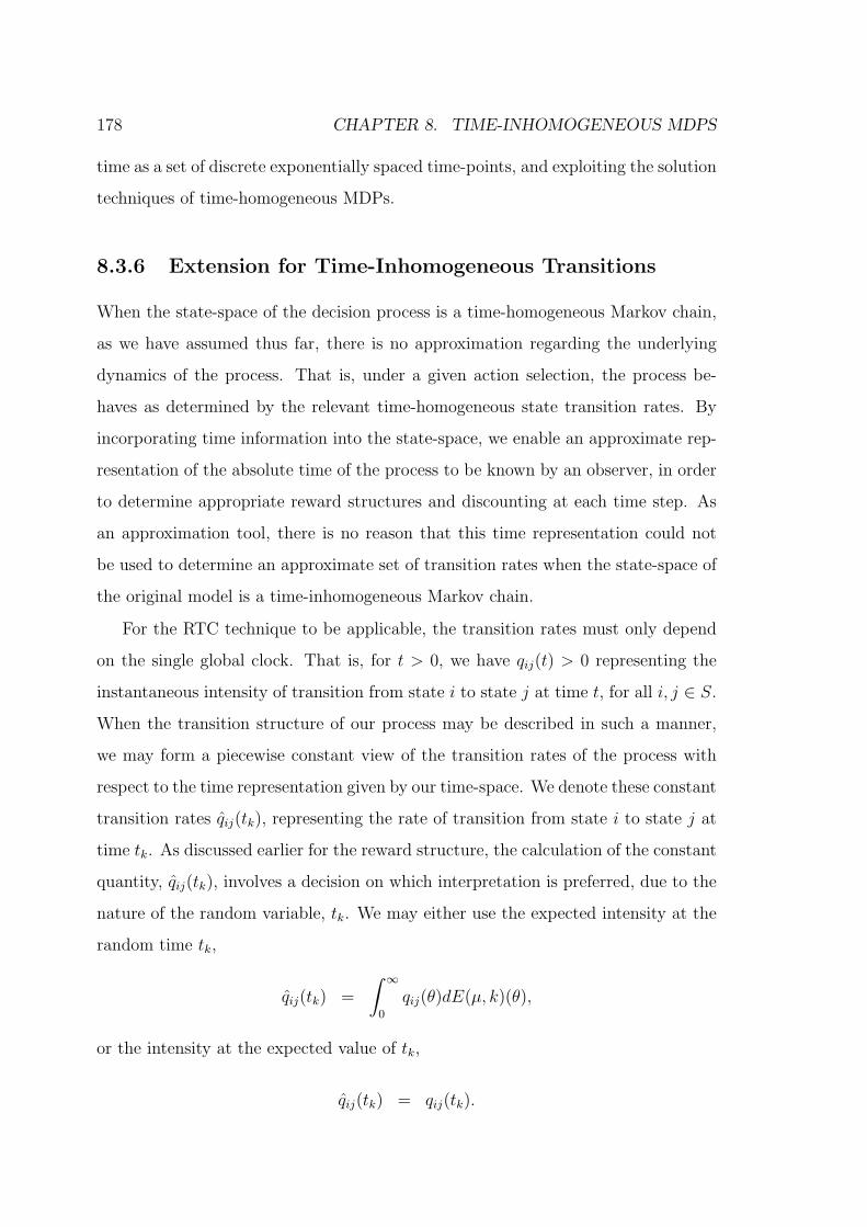
178 CHAPTER 8. TIME-INHOMOGENEOUS MDPS
time as a set of discrete exponentially spaced time-points, and exploiting the solution
techniques of time-homogeneous MDPs.
8.3.6 Extension for Time-Inhomogeneous Transitions
When the state-space of the decision process is a time-homogeneous Markov chain,
as we have assumed thus far, there is no approximation regarding the underlying
dynamics of the process. That is, under a given action selection, the process be-
haves as determined by the relevant time-homogeneous state transition rates. By
incorporating time information into the state-space, we enable an approximate rep-
resentation of the absolute time of the process to be known by an observer, in order
to determine appropriate reward structures and discounting at each time step. As
an approximation tool, there is no reason that this time representation could not
be used to determine an approximate set of transition rates when the state-space of
the original model is a time-inhomogeneous Markov chain.
For the RTC technique to be applicable, the transition rates must only depend
on the single global clock. That is, for t > 0, we have qij(t) > 0 representing the
instantaneous intensity of transition from state i to state j at time t, for all i, j ∈ S.
When the transition structure of our process may be described in such a manner,
we may form a piecewise constant view of the transition rates of the process with
respect to the time representation given by our time-space. We denote these constant
transition rates qij(tk), representing the rate of transition from state i to state j at
time tk. As discussed earlier for the reward structure, the calculation of the constant
quantity, qij(tk), involves a decision on which interpretation is preferred, due to the
nature of the random variable, tk. We may either use the expected intensity at the
random time tk,
qij(tk) =
∫ ∞
0
qij(θ)dE(µ, k)(θ),
or the intensity at the expected value of tk,
qij(tk) = qij(tk).
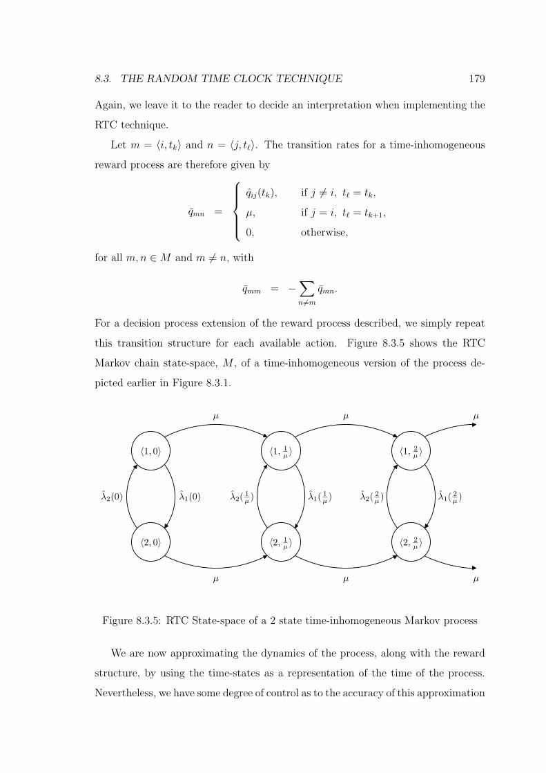
8.3. THE RANDOM TIME CLOCK TECHNIQUE 179
Again, we leave it to the reader to decide an interpretation when implementing the
RTC technique.
Let m = 〈i, tk〉 and n = 〈j, tℓ〉. The transition rates for a time-inhomogeneous
reward process are therefore given by
qmn =
qij(tk), if j 6= i, tℓ = tk,
µ, if j = i, tℓ = tk+1,
0, otherwise,
for all m,n ∈M and m 6= n, with
qmm = −∑
n6=m
qmn.
For a decision process extension of the reward process described, we simply repeat
this transition structure for each available action. Figure 8.3.5 shows the RTC
Markov chain state-space, M , of a time-inhomogeneous version of the process de-
picted earlier in Figure 8.3.1.
〈1, 0〉
〈2, 0〉
λ1(0)λ2(0)
〈1, 1
µ〉
〈2, 1
µ〉
λ1(1
µ)λ2(
1
µ)
〈1, 2
µ〉
〈2, 2
µ〉
λ1(2
µ)λ2(
2
µ)
µ µ
µ µ µ
µ
Figure 8.3.5: RTC State-space of a 2 state time-inhomogeneous Markov process
We are now approximating the dynamics of the process, along with the reward
structure, by using the time-states as a representation of the time of the process.
Nevertheless, we have some degree of control as to the accuracy of this approximation

180 CHAPTER 8. TIME-INHOMOGENEOUS MDPS
with respect to selection of the time-space. To demonstrate the RTC technique, we
will now consider a familiar time-homogeneous decision process, the race, with the
added complexity of time-inhomogeneous discounting.
8.4 The Race – Erlang System
In this section, we implement the RTC technique for the solution of an Erlang race
with non-exponential discounting. We have chosen the Erlang race for the purpose
of demonstration, as the transition structure can actually be formulated as that
of a time-inhomogeneous Markov chain. This is not, in general, possible for time-
homogeneous semi-Markov decision processes, and we will discuss the applicability
of our RTC technique in more general terms in Section 8.5. The combination of the
concurrency of the holding time distributions and the acyclic nature of the state-
space enables us to model all aspects of the actual system with reference to a single
global clock. Thus, the Erlang race is a suitable, and suitably complex, process to
demonstrate the effectiveness of the RTC technique.
Note, however, that our RTC technique can handle Markov state-spaces that are
far more complex than that of the simple acyclic state-space of the race. We are
nevertheless endeavouring to provide a comparison between our technique and the
solution found directly from the corresponding integral value equations. It is in fact
the value equation solution that provides the bottleneck for the complexity of the
processes that we could select for this demonstration. A cyclic state-space would
result in a system of value equations which are extremely difficult, if at all possible,
to solve.
The process to which we will apply our RTC technique is a race consisting of a
system of 3 identical Erlang order 2 distributions with rate parameter λ = 3. The
state-space of this system is S = {−1, 0, 1, 2, 3}, where state i = −1 corresponds
to the introduced termination state required for the aforementioned decision pro-
cess. In Section 4.4.3, it was shown that the race, although originally described
as a GSMDP, could be formulated as a time-inhomogeneous SMDP, as all of the
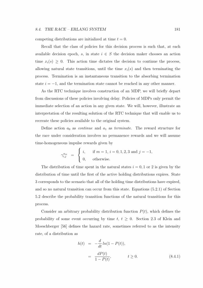
8.4. THE RACE – ERLANG SYSTEM 181
competing distributions are initialized at time t = 0.
Recall that the class of policies for this decision process is such that, at each
available decision epoch, s, in state i ∈ S the decision maker chooses an action
time xi(s) ≥ 0. This action time dictates the decision to continue the process,
allowing natural state transitions, until the time xi(s) and then terminating the
process. Termination is an instantaneous transition to the absorbing termination
state i = −1, and the termination state cannot be reached in any other manner.
As the RTC technique involves construction of an MDP, we will briefly depart
from discussions of these policies involving delay. Policies of MDPs only permit the
immediate selection of an action in any given state. We will, however, illustrate an
interpretation of the resulting solution of the RTC technique that will enable us to
recreate these policies available to the original system.
Define action a0 as continue and a1 as terminate. The reward structure for
the race under consideration involves no permanence rewards and we will assume
time-homogeneous impulse rewards given by
γam
i,j =
i, if m = 1, i = 0, 1, 2, 3 and j = −1,
0, otherwise.
The distribution of time spent in the natural states i = 0, 1 or 2 is given by the
distribution of time until the first of the active holding distributions expires. State
3 corresponds to the scenario that all of the holding time distributions have expired,
and so no natural transition can occur from this state. Equations (5.2.1) of Section
5.2 describe the probability transition functions of the natural transitions for this
process.
Consider an arbitrary probability distribution function P (t), which defines the
probability of some event occurring by time t, t ≥ 0. Section 2.3 of Klein and
Moeschberger [56] defines the hazard rate, sometimes referred to as the intensity
rate, of a distribution as
h(t) = − d
dtln(1− P (t)),
=dP (t)
1− P (t), t ≥ 0. (8.4.1)

182 CHAPTER 8. TIME-INHOMOGENEOUS MDPS
This rate can be interpreted as the instantaneous rate of expiration of the distribu-
tion P (t) at time t. The use of this rate is popular in survival analysis and it has
appeared in a variety of models, ranging from those relating to medical issues such
as in Keiding and Andersen [54] to those involving fast simulation of computing
systems, as in Nicola, Heidelberger and Shahabuddin [68]. More recently, Aalen
and Gjessing [2] provided insight into the shape of various hazard rates, as time is
varied, from a Markov process perspective.
We derive, using equations (5.2.1) in conjunction with equation (8.4.1), time-
inhomogeneous intensity rates of natural transitions given by
ha0i,i+1(t) =
(3− i)λrtr−1
(r − 1)!r−1∑
j=0
(λt)j
j!
, (8.4.2)
=(3− i)9t
1 + 3t, for i = 0, 1, 2, and t ≥ 0. (8.4.3)
These rates, as they depend only on the absolute time of the process, form the
framework for the instantaneous transition rates of a time-inhomogeneous Markov
process modelling the natural transitions of the race.
We define an infinitesimal generator Q0(t) = [qa0ij (t)] of the transitions of the
process under selection of action a0 where
qa0i,j(t) =
ha0i,i+1(t), if i = 0, 1, 2 and j = i + 1,
0, otherwise,
for all i, j ∈ S. We also define an infinitesimal generator for the process when action
a1 is selected, Q1(t) = [qa1ij (t)]. The elements of Q1(t) are given by
qa1i,j(t) =
α, if i 6= −1 and j = −1,
0, otherwise,
for all i, j ∈ S, where α is sufficiently large to model an instantaneous transition to
the termination state. A detailed description of the requirements of α to meet this
criteria is given in Section 4.5.2 and so we do not repeat it here. Figures 8.4.1 and
8.4.2 show the continuous-time Markov chains defined by each of the infinitesimal
generators Q0(t) and Q1(t) respectively.
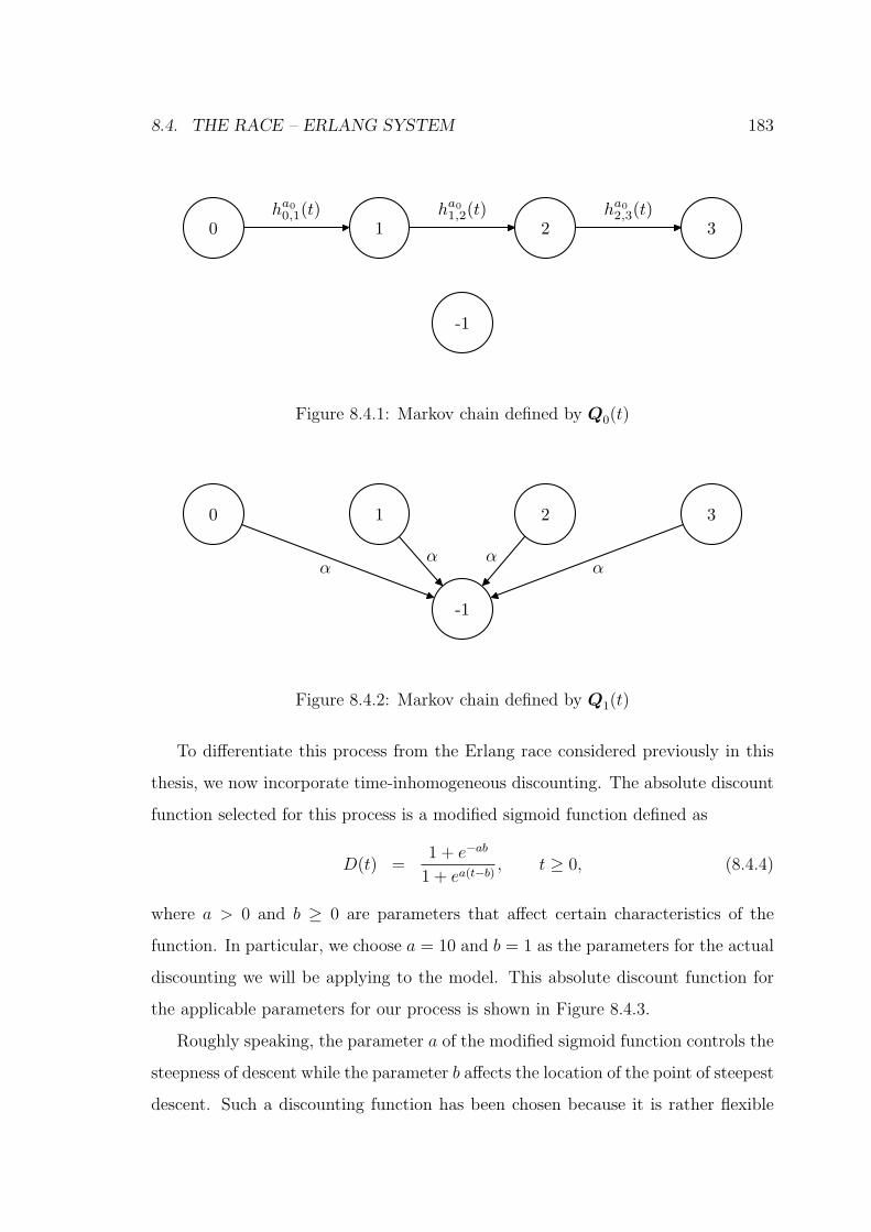
8.4. THE RACE – ERLANG SYSTEM 183
0 1 2 3
-1
ha0
0,1(t) ha0
1,2(t) ha0
2,3(t)
Figure 8.4.1: Markov chain defined by Q0(t)
0 1 2 3
-1
αα α
α
Figure 8.4.2: Markov chain defined by Q1(t)
To differentiate this process from the Erlang race considered previously in this
thesis, we now incorporate time-inhomogeneous discounting. The absolute discount
function selected for this process is a modified sigmoid function defined as
D(t) =1 + e−ab
1 + ea(t−b), t ≥ 0, (8.4.4)
where a > 0 and b ≥ 0 are parameters that affect certain characteristics of the
function. In particular, we choose a = 10 and b = 1 as the parameters for the actual
discounting we will be applying to the model. This absolute discount function for
the applicable parameters for our process is shown in Figure 8.4.3.
Roughly speaking, the parameter a of the modified sigmoid function controls the
steepness of descent while the parameter b affects the location of the point of steepest
descent. Such a discounting function has been chosen because it is rather flexible

184 CHAPTER 8. TIME-INHOMOGENEOUS MDPS
0 0.2 0.4 0.6 0.8 1 1.2 1.4 1.6 1.8 20
0.1
0.2
0.3
0.4
0.5
0.6
0.7
0.8
0.9
1Modified−Sigmoid Discount Function
t
D(t
)
Figure 8.4.3: Sigmoid absolute discount function with parameters a = 10 and b = 1
with regard to modelling the characteristics of processes that are similar to the VoIP
process described in Section 8.2. That is, those processes that maintain their value
quite well, until some absolute time point at which the rate of proportional decrease
in value becomes quite high. This flexibility can be rather useful from a general
modelling perspective.
With the inclusion of the discounting function, we have now completely described
a time-inhomogeneous Markov decision process. Therefore, we may begin imple-
menting the RTC technique to approximate the optimal solution for this decision
process.
The first step is to determine an appropriate time-space for the technique. The
construction of T involves two major considerations: the time of truncation tH and
the rate of transition between the time states. Focusing on the truncation time,
we must observe the nature of the time-inhomogeneous components of our model,
which in this system are the discount function and natural transition rates.
Considering the discount function, we have that D(t)→ ke−at as t→∞, where
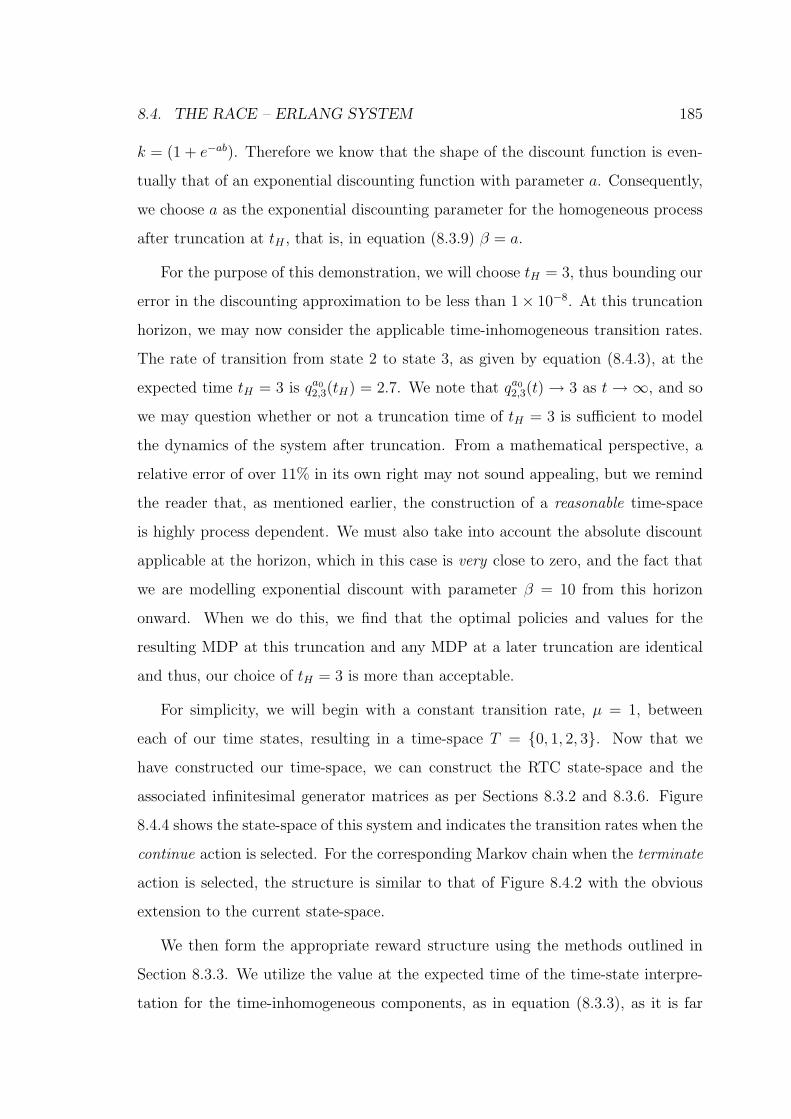
8.4. THE RACE – ERLANG SYSTEM 185
k = (1 + e−ab). Therefore we know that the shape of the discount function is even-
tually that of an exponential discounting function with parameter a. Consequently,
we choose a as the exponential discounting parameter for the homogeneous process
after truncation at tH , that is, in equation (8.3.9) β = a.
For the purpose of this demonstration, we will choose tH = 3, thus bounding our
error in the discounting approximation to be less than 1× 10⁻⁸. At this truncation
horizon, we may now consider the applicable time-inhomogeneous transition rates.
The rate of transition from state 2 to state 3, as given by equation (8.4.3), at the
expected time tH = 3 is qa02,3(tH) = 2.7. We note that qa0
2,3(t)→ 3 as t→∞, and so
we may question whether or not a truncation time of tH = 3 is sufficient to model
the dynamics of the system after truncation. From a mathematical perspective, a
relative error of over 11% in its own right may not sound appealing, but we remind
the reader that, as mentioned earlier, the construction of a reasonable time-space
is highly process dependent. We must also take into account the absolute discount
applicable at the horizon, which in this case is very close to zero, and the fact that
we are modelling exponential discount with parameter β = 10 from this horizon
onward. When we do this, we find that the optimal policies and values for the
resulting MDP at this truncation and any MDP at a later truncation are identical
and thus, our choice of tH = 3 is more than acceptable.
For simplicity, we will begin with a constant transition rate, µ = 1, between
each of our time states, resulting in a time-space T = {0, 1, 2, 3}. Now that we
have constructed our time-space, we can construct the RTC state-space and the
associated infinitesimal generator matrices as per Sections 8.3.2 and 8.3.6. Figure
8.4.4 shows the state-space of this system and indicates the transition rates when the
continue action is selected. For the corresponding Markov chain when the terminate
action is selected, the structure is similar to that of Figure 8.4.2 with the obvious
extension to the current state-space.
We then form the appropriate reward structure using the methods outlined in
Section 8.3.3. We utilize the value at the expected time of the time-state interpre-
tation for the time-inhomogeneous components, as in equation (8.3.3), as it is far
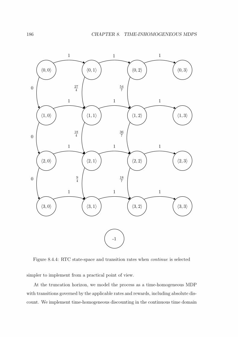
186 CHAPTER 8. TIME-INHOMOGENEOUS MDPS
〈0, 0〉
〈1, 0〉
〈2, 0〉
〈3, 0〉
〈0, 3〉
〈1, 3〉
〈2, 3〉
〈3, 3〉
〈0, 2〉
〈1, 2〉
〈2, 2〉
〈3, 2〉
〈0, 1〉
〈1, 1〉
〈2, 1〉
〈3, 1〉
1 1 1
-1
1 1 1
1 1 1
1 1 1
0
0
0 9
4
18
7
18
4
27
4
36
7
54
7
Figure 8.4.4: RTC state-space and transition rates when continue is selected
simpler to implement from a practical point of view.
At the truncation horizon, we model the process as a time-homogeneous MDP
with transitions governed by the applicable rates and rewards, including absolute dis-
count. We implement time-homogeneous discounting in the continuous time domain

8.4. THE RACE – ERLANG SYSTEM 187
with parameter β = 10, approximating the tail behaviour of the sigmoid discount-
ing in the original process. Following the method outlined in Section 8.3.4 for MDP
truncation, the RTC states 〈i, tH〉, for i = 0, 1, 2, 3, are absorbing and we value them
according to the optimal solution found for the aforementioned time-homogeneous
MDP.
Table 8.4.1 shows the rewards received upon termination from each of the states
of the RTC state-space. Recall that there is no reward to be received when con-
tinue is selected, and thus Table 8.4.1 describes the entire reward structure for this
particular process. The rewards for the non-horizon states are simply the number
of arrived particles multiplied by the absolute discount. At the truncation horizon,
the rewards are the optimal truncation MDP values, also discounted accordingly.
Table 8.4.1: Termination rewards for the RTC state-space
State Reward State Reward State Reward State Reward
〈0, 0〉 0 〈0, 1〉 0 〈0, 2〉 0 〈0, 3〉 9.4× 10⁻¹⁰
〈1, 0〉 1 〈1, 1〉 0.5 〈1, 2〉 4.5× 10⁻⁵ 〈1, 3〉 2.1× 10⁻⁹
〈2, 0〉 2 〈2, 1〉 1 〈2, 2〉 9× 10⁻⁵ 〈2, 3〉 4.2× 10⁻⁹
〈3, 0〉 3 〈3, 1〉 1.5 〈3, 2〉 1.35× 10⁻⁴ 〈3, 3〉 6.3× 10⁻⁹
We have now defined a time-homogeneous continuous-time finite-state MDP on
the RTC state-space, M , which models our infinite horizon time-inhomogeneous
process. We may then solve this process by first discretizing the process via uni-
formization and then solving the resulting Bellman-Howard optimality equations.
Using a time-state transition rate of µ = 1 is obviously not going to approx-
imate the original model very accurately, as there are large changes of the time-
inhomogeneous components from one time-state to the next. For the following anal-
ysis, we set µ = 100 in an attempt to more accurately capture the dynamics of the
system. We follow all of the aforementioned steps in the construction of the MDP on
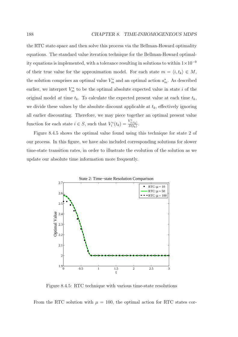
188 CHAPTER 8. TIME-INHOMOGENEOUS MDPS
the RTC state-space and then solve this process via the Bellman-Howard optimality
equations. The standard value iteration technique for the Bellman-Howard optimal-
ity equations is implemented, with a tolerance resulting in solutions to within 1×10⁻⁹
of their true value for the approximation model. For each state m = 〈i, tk〉 ∈ M ,
the solution comprises an optimal value V ∗m and an optimal action a∗
m. As described
earlier, we interpret V ∗m to be the optimal absolute expected value in state i of the
original model at time tk. To calculate the expected present value at each time tk,
we divide these values by the absolute discount applicable at tk, effectively ignoring
all earlier discounting. Therefore, we may piece together an optimal present value
function for each state i ∈ S, such that V ∗i (tk) =
V ∗〈i,tk〉
D(tk).
Figure 8.4.5 shows the optimal value found using this technique for state 2 of
our process. In this figure, we have also included corresponding solutions for slower
time-state transition rates, in order to illustrate the evolution of the solution as we
update our absolute time information more frequently.
0 0.5 1 1.5 2 2.5 31.9
2
2.1
2.2
2.3
2.4
2.5
2.6
2.7State 2: Time−state Resolution Comparison
t
Opt
imal
Val
ue
RTC: µ = 10RTC: µ = 50RTC: µ = 100
Figure 8.4.5: RTC technique with various time-state resolutions
From the RTC solution with µ = 100, the optimal action for RTC states cor-
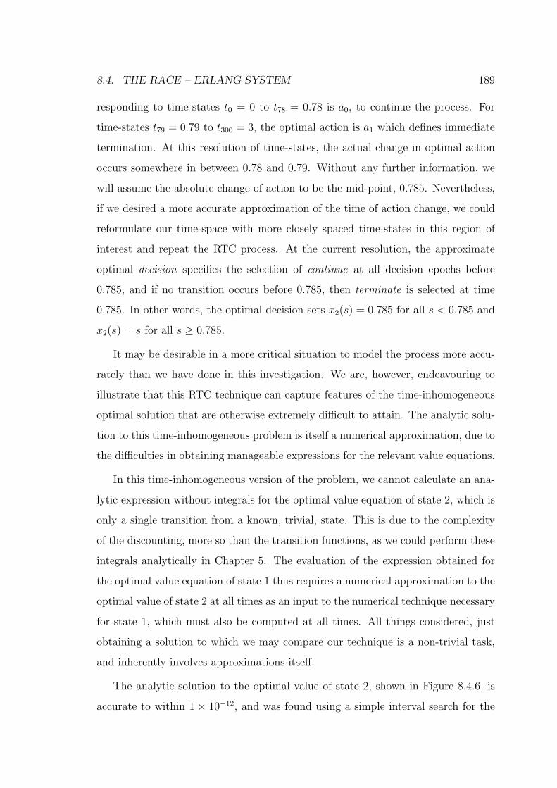
8.4. THE RACE – ERLANG SYSTEM 189
responding to time-states t0 = 0 to t78 = 0.78 is a0, to continue the process. For
time-states t79 = 0.79 to t300 = 3, the optimal action is a1 which defines immediate
termination. At this resolution of time-states, the actual change in optimal action
occurs somewhere in between 0.78 and 0.79. Without any further information, we
will assume the absolute change of action to be the mid-point, 0.785. Nevertheless,
if we desired a more accurate approximation of the time of action change, we could
reformulate our time-space with more closely spaced time-states in this region of
interest and repeat the RTC process. At the current resolution, the approximate
optimal decision specifies the selection of continue at all decision epochs before
0.785, and if no transition occurs before 0.785, then terminate is selected at time
0.785. In other words, the optimal decision sets x2(s) = 0.785 for all s < 0.785 and
x2(s) = s for all s ≥ 0.785.
It may be desirable in a more critical situation to model the process more accu-
rately than we have done in this investigation. We are, however, endeavouring to
illustrate that this RTC technique can capture features of the time-inhomogeneous
optimal solution that are otherwise extremely difficult to attain. The analytic solu-
tion to this time-inhomogeneous problem is itself a numerical approximation, due to
the difficulties in obtaining manageable expressions for the relevant value equations.
In this time-inhomogeneous version of the problem, we cannot calculate an ana-
lytic expression without integrals for the optimal value equation of state 2, which is
only a single transition from a known, trivial, state. This is due to the complexity
of the discounting, more so than the transition functions, as we could perform these
integrals analytically in Chapter 5. The evaluation of the expression obtained for
the optimal value equation of state 1 thus requires a numerical approximation to the
optimal value of state 2 at all times as an input to the numerical technique necessary
for state 1, which must also be computed at all times. All things considered, just
obtaining a solution to which we may compare our technique is a non-trivial task,
and inherently involves approximations itself.
The analytic solution to the optimal value of state 2, shown in Figure 8.4.6, is
accurate to within 1 × 10⁻¹², and was found using a simple interval search for the

190 CHAPTER 8. TIME-INHOMOGENEOUS MDPS
unique non-trivial zero of its derivative corresponding to a maximum. Unlike the
earlier races in this thesis, a manageable expression demonstrating the uniqueness of
this zero was not available in general, but for the system parameters used within this
section, the uniqueness can be guaranteed. Figure 8.4.6 shows the comparison be-
tween the solutions found directly from the value equations and our RTC technique
with µ = 100. The relative error of the RTC technique compared to the solution
found using the value equations is then shown in Figure 8.4.7, where we see that the
maximum error of our RTC technique is just above 0.25% for this particular process
and reduces very quickly with time.
0 0.5 1 1.5 2 2.5 30
0.5
1
1.5
2
2.5
3State 2: Technique Comparison
t
Opt
imal
Val
ue
Value EquationsRTC: µ = 100
Figure 8.4.6: Technique comparison for optimal value of state 2
Figure 8.4.8 shows the optimal solutions found for the integral value equations
and the RTC technique corresponding to state 1 of the original process. As it
was hinted earlier, the effort expended to find this analytic solution was great.
In the absence of neat analytic expressions for state 2, the associated optimality
equations for level 1 become almost unmanageable. As many simplifications as
possible, regarding the nature of possible optimal solutions for this process, were

8.4. THE RACE – ERLANG SYSTEM 191
0 0.5 1 1.5 2 2.5 30
0.5
1
1.5
2
2.5
3x 10
−3 Relative Error for RTC Technique
t
Rel
ativ
e E
rror
Figure 8.4.7: Absolute error of the RTC technique for state 2
implemented. Even then, the computation time spent to produce the data in Figure
8.4.8, which is only at a resolution of 100 time-steps per unit of time, was just
under 6 hours on a dedicated processing machine. To formulate a general technique
for a solution in this manner for a general process would be a monumental task,
particularly if a solution is desired in a reasonable amount of time.
The author makes no claim that the computer code used to generate the value
equation solution of Figure 8.4.8 is as efficient as it could be, although every effort
was made to reduce the computation time. The time taken to solve the corre-
sponding problem using the implemented RTC technique, however, is just under 30
seconds, for the entire process. Whether direct solution of the value equations could
be streamlined for performance is a separate issue. Nevertheless, it is highly unlikely
that any improvements would cause a decrease in computation time to that similar
to the RTC technique.

192 CHAPTER 8. TIME-INHOMOGENEOUS MDPS
0 0.5 1 1.5 2 2.5 30
0.5
1
1.5
2
2.5
3State 1: Technique Comparison
t
Opt
imal
Val
ue
Value EquationsRTC: µ = 100
Figure 8.4.8: Technique comparison for optimal value of state 1
8.5 Summary
The RTC technique developed in this chapter is a technique for the approximation
of optimal solutions of a class of time-inhomogeneous Markov decision processes.
This class is defined by all processes whose time-inhomogeneous components can
be determined with reference to a single global clock. These time-inhomogeneous
components may be reward related, such as permanence and impulse rewards and
discounting, and transition intensity related.
We have given an example in the previous section of the technique applied to
a time-inhomogeneous SMDP. This process belongs to the class of suitable MDPs
for this technique, because it can be reformulated in continuous-time as a time-
inhomogeneous MDP using intensity rates to model the transition dynamics. This
is a useful technique to handle non-exponential distributions, provided every distri-
bution in the system is defined by a single global clock. As a consequence, a general
SMDP is not suitable for the RTC technique due to the renewal of the holding
time distributions each time a state is entered. This is unless the reward struc-
8.5. SUMMARY 193
ture possesses features such that, for example, the model permits value resetting on
transitions.
As such, the RTC technique is applicable to any process that can be approx-
imated as a continuous-time MDP, with time information incorporated into the
state-space and an appropriate reward structure. Exactly how to construct the re-
ward and transition structure in general for processes with unusual features is highly
model dependent. Thus the applicability of the RTC technique should be considered
on a case by case basis, for any model outside the class whose dynamics and value
can be described by a single global clock.
As an approximation technique, the RTC technique is easy to implement for
general processes belonging to the aforementioned class. It is tunable with regard to
accuracy via the resolution and horizon of the time-space. We note that the resolu-
tion need not be consistent over the entirety of the time-space. Thus, certain regions
may receive more attention in the modelling process, while others that require less,
may receive less. It is therefore a reasonable, and certainly fast, approximation
technique for the solution of a large class of practical decision processes, in a field
where very little pertaining to such solutions exists in the literature to date.


Chapter 9
Conclusions
In this thesis, we have investigated the complexity of solution of various classes
of time-dependent Markovian decision process and, where possible, have developed
original techniques to address this complexity. These two original techniques each
apply to their own specific class of decision processes, but we note that these classes
can themselves be difficult to characterize. Nevertheless, when applicable, the tech-
niques offer an alternative to the direct treatment of the general value equations of
Chapter 4 that has the definite potential to reduce the complexity of the solution
process.
Chapter 5 contains an in-depth analysis of a particular Markovian decision pro-
cess, that of the Erlang race, via consideration of the general value equations. We
began by investigating properties of the optimal solution for certain states of the
process. However, noting that the value equations are incredibly complex in gen-
eral, we showed that even for a process as simply stated as the race, the analytic
optimal solution for certain states of the system was very difficult to obtain. The
analysis in this chapter provided a good insight into the difficulties of dealing with
the value equations directly, along with a benchmark against which to compare our
first original technique.
In Chapter 6, we gave an initial introduction to the phase-space model of a
process by considering the Erlang race of the previous chapter. Utilizing the PH
representation of the Erlang distribution, a new phase-space was constructed, effec-
195

196 CHAPTER 9. CONCLUSIONS
tively modelling the state-space of the original process as a continuous-time Markov
process. This idea of incorporating the phases into the state-space of a process is a
relatively new concept, with examples found by the author only in Younes and Sim-
mons [96] and Younes [95] in 2004 and 2005 respectively. When valuing this newly
formed process, one must nevertheless be cautious, as the phases are not visible in
the original model. Younes [95] claims to have addressed this issue, but we show
that there is a fundamental flaw in his valuation of the states of the phase-space.
We correct for this flaw by introducing an original action-consistent valuation
technique for the states of the phase-space. Using transient analysis techniques, we
then reconstruct the optimal solution for our original Erlang race from the solution
obtained for the phase-space model. Due to the nature of the state-space of the
Erlang race, we are able to solve this process, state by state, using a top-down
approach similar to that of dynamic programming. As an added feature in the
phase-space technique, we identified certain characteristics of an optimal solution of
a state that, when applicable, greatly simplified the implementation of our phase-
space technique.
Chapter 7 further developed the phase-space model construction and solution
technique in a more general setting for SMDPs, building on the theory outlined in
the previous chapter. Accounting for the added complexity of general processes, we
defined an original system of value equations for this phase-space that are equivalent
to those for SMDPs outlined in Chapter 4, when the class of policies are such that
actions must be selected immediately upon entering a state.
These newly defined value equations for the phase-space, however, are potentially
as complex as those defined for the original model. As a topic for future research,
it is possible that, given the restricted policy class, the original value equations for
certain systems may be solved using a fixed-point policy iteration algorithm. If
so, the phase-space value equations of an equivalent system may also be amenable
to solution via policy iteration. It is nevertheless not clear whether a fixed-point
iteration algorithm for policy iteration would perform better for either system, and
we see this line of investigation as another topic for further research.

197
We then restricted our focus to systems with acyclic state-spaces, in order to
enable a top-down solution approach. As for the specific Erlang race, we identified
characteristics of an optimal solution to look for when implementing this technique.
For the situations where these solution characteristics are present in the system, we
provided simplifications of the value equations that greatly reduce the complexity
of the phase-space technique. It is almost impossible, however, to determine a
priori the class of processes for which the simplifications outlined in our phase-space
technique will be applicable. Nevertheless, as these phase-space value equations and
those of Chapter 4 are identical, we do no worse, in terms of complexity, by utilizing
our phase-space technique, and leave open the opportunity to simplify the solution
process if an appropriate situation arises.
There is potential for these simplifications to apply in processes without acyclic
state-spaces. To use these simplifications for such processes, we firstly require a
solution technique for the value equations less complex than direct evaluation. For
this purpose, a fixed point iteration technique for the value equations, as mentioned
earlier as a topic for further research, would suffice. Without an obvious identi-
fication tool for the presence of suitable characteristics, such as the level by level
approach available to acyclic systems, it is not clear how the simplifications would
apply in the solution process and we leave this aspect as another topic for future
research.
The solution technique developed in Chapter 8 is an approximation technique
for the solution of the class of infinite horizon decision processes whose state transi-
tions and reward structures, including discounting, can be described with reference
to a single global clock. We noted that such time-dependence, particularly that of
time-inhomogeneous discounting of the process, appears very rarely in the literature.
This random time clock (RTC) technique represented time using exponentially dis-
tributed length intervals and incorporated this absolute time information into an
expanded state-space. To model the transition dynamics of processes where the
state-transitions are not exponentially distributed, we used the hazard rates of the
transition probability distributions evaluated according to this time representation.

198 CHAPTER 9. CONCLUSIONS
A suitable reward structure approximation, again using our time representation, was
given, along with guidelines for sensible truncation using an MDP approximation to
the tail behaviour of the original infinite horizon process.
The result of this process is a finite-state time-homogeneous MDP approxima-
tion to the original process. This MDP may be solved using standard existing
solution techniques and we provided an interpretation of the results such that the
approximation to the solution to the original process can be retrieved. An exam-
ple of the Erlang race with time-dependent discounting was given to demonstrate
this approximation technique and the results were compared with those obtained,
where possible, directly from the value equations. It was shown that this approx-
imation technique performs admirably with respect to speed and accuracy for the
given example.
While these original techniques provide an avenue for the solution of compli-
cated Markovian decision processes, the major contribution of this thesis lies in
the progression of their development. Each technique utilizes a variety of existing
Markovian process analysis tools to derive an alternative or approximate system
to the process being modelled. In tying together these ideas and concepts, regard-
ing different aspects of the process under consideration, in original and novel ways,
the resulting systems are more amenable to solution for optimality. We note that
the applicable classes to which our techniques apply may be somewhat restrictive.
Nevertheless, in the absence of practical solution techniques, there is potential to
draw upon the modelling utilized throughout this thesis to formulate new solution
techniques for more general, and more complex, Markovian decision processes.

References
[1] O. O. Aalen. On phase-type distributions in survival analysis. Scandinavian
Journal of Statistics, 22(4):447–463, 1995.
[2] O. O. Aalen and H. K. Gjessing. Understanding the shape of the hazard rate:
A process point of view. Statistical Science, 16(1):1–14, 2001.
[3] J. M. Alden and R. L. Smith. Rolling horizon procedures in nonhomogeneous
Markov decision processes. Operations Research, 40(Supp. 2):S183–S194, 1992.
[4] S. Asmussen, F. Avram, and M. Usabel. Erlangian approximations for finite
time ruin probabilities. ASTIN Bulletin, 32(2):267–281, 2002.
[5] S. Asmussen, O. Nerman, and M. Olsson. Fitting phase-type distributions via
the EM algorithm. Scandinavian Journal of Statistics, 23(4):419–441, 1996.
[6] S. Asmussen and M. Olsson. Phase type distributions (update). In S. Kotz,
C. B. Read, and D. L. Banks, editors, Encyclopedia of Statistical Science Up-
date, volume 2, pages 525–530. New York: John Wiley & Sons, 1998.
[7] A. D. Barbour. Generalized semi-Markov schemes and open queuing networks.
Journal of Applied Probability, 19:469–474, 1982.
[8] J. C. Bean, R. L. Smith, and J.-B. Lasserre. Denumerable state nonhomoge-
neous Markov decision processes. Journal of Mathematical Analysis and Appli-
cation, 153:64–77, 1990.
[9] N. G. Bean and D. A. Green. When is a MAP poisson? Mathematical and
Computer Modelling, 31:31–46, 2000.
199

[10] N. G. Bean, N. Kontoleon, and P. G. Taylor. Markovian trees: Properties and
algorithms. Annals of Operations Research, Special issue on Matrix-Analytic
methods in Stochastic Modelling, 160(1):31–50, 2008.
[11] A. Bellen, Z. Jackiewicz, R. Vermiglio, and M. Zennaro. Natural continuous
extensions of Runge-Kutta methods for Volterra integral equations of the second
kind and their applications. Mathematics of Computation, 52(185):49–63, 1989.
[12] R. E. Bellman. Dynamic Programming. Princeton : Princeton University Press,
1957.
[13] D. P. Bertsekas. Dynamic Programming and Stochastic Control. Academic
Press, 1976.
[14] A. Bobbio and M. Telek. A benchmark for PH estimation algorithms: Results
for acyclic-PH. Communications in Statistics: Stochastic models, 10(3):661–
667, 1994.
[15] R. F. Botta, C. M. Harris, and W. G. Marchal. Characterizations of gener-
alized hyper-exponential distribution functions. Communications in Statistics:
Stochastic Models, 3(1):115–148, 1987.
[16] J. A. Boyan and M. L. Littman. Exact solutions to time-dependent MDPs.
In T. K. Leen, T. G. Dietterich, and V. Tresp, editors, Advances in Neural
Information Processing Systems 13, pages 1026–1032, Denver, Colorado, USA,
November 2000.
[17] J. A. Boyan and M. L. Littman. Representations and algorithms for exact time-
dependent MDPs. In 16th Conference in Uncertainty in Artificial Intelligence:
Beyond MDPs Workshop, Stanford, California, USA, 2000.
[18] B. J. Cairns, J. V. Ross, and T. Taimre. Models for predicting extinction times:
shall we dance (or walk or jump)? In Proceedings of the 16th Biennial Congress
on Modelling and Simulation (MODSIM05), pages 2061–2067. Modelling and
Simulation Society of Australia and New Zealand, 2005.
200

[19] L. Cantaluppi. Computation of optimal policies in discounted semi-Markov
decision chains. OR Spektrum, 6:147–160, 1984.
[20] E. Cinlar. Markov renewal theory. Advances in Applied Probability, 1:123–187,
1969.
[21] E. Cinlar. Introduction to Stochastic Processes. Prentice Hall, 1975.
[22] C. Commault and J. P. Chemla. On dual and minimal phase-type representa-
tions. Communications in Statistics: Stochastic Models, 9(3):421–434, 1993.
[23] C. Commault and J. P. Chemla. An invariant of representations of phase-type
distributions and some applications. Journal of Applied Probability, 33(2):368–
381, 1996.
[24] A. J. Coyle and P. G. Taylor. Tight bounds on the sensitivity of generalised
semi-Markov processes with a single generally distributed lifetime. Journal of
Applied Probability, 32:63–73, 1995.
[25] T. K. Das, A. Gosavi, S. Mahadevan, and N. Marchalleck. Solving semi-Markov
decision problems using average reward reinforcement learning. Management
Science, 45(4):560–574, 1999.
[26] R. De Dominicis and R. Manca. An algorithmic approach to non-homogeneous
semi-Markov processes. Communications in Statistics: Simulation and Com-
putation, 13(6):823–838, 1984.
[27] B. T. Doshi. Generalized semi-Markov decision processes. Journal of Applied
Probability, 16(3):618–630, 1979.
[28] A. K. Erlang. Solution of some problems in the theory of probabilities of signif-
icance in automatic telephone exchanges. The Post Office Electrical Engineer’s
Journal, 10:189–197, 1917.
201

[29] M. J. Faddy. On inferring the number of phases in a Coxian phase-type dis-
tribution. Communications in Statistics: Stochastic Models, 14(1&2):407–417,
1998.
[30] P. Fazekas, S. Imre, and M. Telek. Modeling and analysis of broadband cellu-
lar networks with multimedia connections. Telecommunication Systems, 19(3–
4):263–288, 2002.
[31] E. A. Feinberg. Constrained discounted semi-Markov decision processes. In
Z. Hou, J. A. Filar, and A. Chen, editors, Markov Processes and Controlled
Markov Chains, pages 231–242. Dordrecht: Kluwer Academic Publishers, 2002.
[32] K. A. Freedberg, J. A. Scharfstein, G. R. Seage III, E. Losina, M. C. Wein-
stein, D. E. Craven, and A. D. Paltiel. The cost-effectiveness of preventing
AIDS-related opportunistic infections. The Journal of the American Medical
Association, 279:130–136, 1998.
[33] L. Garey. Solving nonlinear second kind Volterra equations by modified incre-
ment methods. SIAM Journal on Numerical Analysis, 12(3):501–508, 1975.
[34] P. Glasserman and D. D. Yao. Monotonicity in generalized semi-Markov pro-
cesses. Mathematics of Operations Research, 17:1–21, 1992.
[35] P. W. Glynn. On the role of generalized semi-Markov processes in simulation
output. In S. Roberts, J. Banks, and B. Schmeiser, editors, Proceedings of the
1983 Winter Simulation Conference, pages 39–42, 1983.
[36] P. W. Glynn. A GSMP formalism for discrete event systems. Proceedings of
the IEEE, 77(1):14–23, 1989.
[37] Q.-M. He, E. M. Jewkes, and J. Buzacott. The value of information used in
inventory control of a make-to-order inventory-production system. IIE Trans-
actions, 34(11):999–1013, 2002.
[38] Q.-M. He and H. Zhang. On matrix exponential distributions. Advances in
Applied Probability, 39(1):271–292, 2007.
202
[39] W. J. Hopp. Identifying forecast horizons in nonhomogeneous Markov decision
processes. Operations Research, 37(2):339–343, 1989.
[40] W. J. Hopp, J. C. Bean, and R. L. Smith. A new optimality criterion for
nonhomogeneous Markov decision processes. Operations Research, 35(6):875–
883, 1987.
[41] R. A. Howard. Dynamic Programming and Markov Processes. Cambridge,
Massachusetts: M. I. T. Press, 1960.
[42] R. A. Howard. Dynamic Probabilistic Systems, Volume I: Markov Models. New
York: John Wiley & Sons, 1971.
[43] R. A. Howard. Dynamic Probabilistic Systems, Volume II: Semi-Markov and
Decision Processes. New York: John Wiley & Sons, 1971.
[44] ITU-T Recommendation G.107. The E-model, a computational model for use
in transmission planning, 2005.
[45] ITU-T Recommendation G.113. Transmission impairments due to speech pro-
cessing, 2007.
[46] ITU-T Recommendation G.114. One-way transmission time, 2003.
[47] J. Janssen and R. De Dominicis. Finite non-homogeneous semi-Markov pro-
cesses: Theoretical and computational aspects. Insurance: Mathematics and
Economics, 3:157–165, 1984.
[48] J. Janssen and R. Manca. Numerical solution of non-homogeneous semi-Markov
processes in transient case. Methodology and Computing in Applied Probability,
3:271–293, 2001.
[49] J. Janssen and R. Manca. Applied Semi-Markov Processes. New York: Springer,
2006.
203

[50] J. Janssen, R. Manca, and E. Volpe di Prignano. Continuous time non homoge-
neous semi-Markov reward processes and multi-state insurance application. In
Proceedings of the 8th International Congress on Insurance: Mathematics and
Economics, Rome, Italy, June 2004.
[51] R. A. Jarrow, D. Lando, and S. M. Turnbull. A Markov model for the term
structure of credit risk spreads. The Review of Financial Studies, 10:481–523,
1997.
[52] A. Jensen. Markoff chains as an aid in the study of Markoff processes. Skandi-
navisk Aktuarietidskrift, 36:87–91, 1953.
[53] L. P. Kaelbling, M. L. Littman, and A. R. Cassandra. Planning and acting
in partially observable stochastic domains. Artificial Intelligence, 101:99–134,
1998.
[54] N. Keiding and P. K. Andersen. Nonparametric estimation of transition inten-
sities and transition probabilities: A case study of a two-state Markov process.
Applied Statistics, 38(2):319–329, 1989.
[55] M. Kijima. Markov Processes for Stochastic Modeling. London: Chapman &
Hall, 1997.
[56] J. P. Klein and M. L. Moeschberger. Survival Analysis: Techniques for Censored
and Truncated Data. New York: Springer, 2nd edition, 2003.
[57] Y. H. Kwon and D. K. Sung. Elevation angle dependent Markov model for LEO
satellite communication systems. In Global Telecommunications Conference
(GLOBECOM), volume 1A, pages 281–285, 1999.
[58] G. Latouche and V. Ramaswami. Introduction to Matrix Analytic Methods in
Stochastic Modelling. SIAM, Philadelphia, 1999.
[59] M. L. Littman, A. R. Cassandra, and L. P. Kaelbling. Learning policies for
partially observable environments: Scaling up. In Proceedings of the Twelfth
204
International Conference on Machine Learning, pages 362–370. Morgan Kauf-
mann publishers Inc.: San Mateo, CA, USA, 1995.
[60] H. Madsen, H. Spliid, and P. Thyregod. Markov models in discrete and continu-
ous time for hourly observations of cloud cover. Journal of Applied Meteorology,
24(7):629–639, 1985.
[61] A. H. Marshall and S. I. McClean. Using Coxian phase-type distributions to
identify patient characteristics for duration of stay in hospital. Health Care
Mangement Science, 7:285–289, 2004.
[62] L. W. McKenzie. Matrices with dominant diagonal in economic theory. In
K. J. Arrow, S. Karlin, and P. Suppes, editors, Mathematical Models in Social
Sciences, pages 47–62. Stanford: Stanford University Press, 1960.
[63] J. McMahon, M. Rumsewicz, P. Boustead, and F. Safaei. Investigation and
modeling of traffic issues in immersive audio environments. In Proceedings of
the International Conference on Communications, Paris, France, June 2004.
[64] G. E. Monahan. A survey of partially observable Markov decision processes:
Theory, models, and algorithms. Management Science, 28(1):1–16, 1982.
[65] M. F. Neuts. Probability distributions of phase type. In Liber Amicorum Prof.
Emeritus H. Florin, pages 173–206. Department of Mathematics, University of
Louvain, Belgium, 1975.
[66] M. F. Neuts. Matrix-geometric Solutions in Stochastic Models : An Algorithmic
Approach. Baltimore: Johns Hopkins University Press, 1981.
[67] M. F. Neuts and K. S. Meier. On the use of phase type distributions in reliability
modelling of systems with two components. OR Spektrum, 2:227–234, 1981.
[68] V. F. Nicola, P. Heidelberger, and P. Shahabuddin. Uniformization and ex-
ponential transformation: Techniques for fast simulation of highly dependable
non-Markovian systems. In Proceedings of the 22nd International Symposium
205
on Fault Tolerant Computing, pages 130–139, Boston, Massachusetts, USA,
July 1992.
[69] C. A. O’Cinneide. On non-uniqueness of representations of phase-type distri-
butions. Communications in Statistics: Stochastic models, 5(2):247–259, 1989.
[70] T. Osogami and M. Horchol-Balter. Necessary and sufficient conditions for
representing general distributions by Coxians. In Computer Performance Eval-
uation / TOOLS, pages 182–199, 2002.
[71] R. Parr and S. Russell. Approximating optimal policies for partially observable
stochastic domains. In Proceedings of the International Joint Conference on
Artificial Intelligence, 1995.
[72] V. Paxson and S. Floyd. Wide area traffic: the failure of Poisson modeling.
IEEE/ACM Transactions on Networking, 3(3):226–244, 1995.
[73] R. Perez-Ocon, J. E. Ruiz-Castro, and M. L. Gamiz-Perez. Non-homogeneous
Markov models in the analysis of survival after breast cancer. Journal of the
Royal Statistical Society: Series C (Applied Statistics), 50(1):111–124, 2001.
[74] M. L. Puterman. Markov Decision Processes : Discrete Stochastic Dynamic
Programming. New York: John Wiley & Sons, 1994.
[75] B. Rajagopalan, U. Lall, and D. G. Tarboton. Non-homogeneous Markov model
for daily precipitation. Journal of Hydrologic Engineering, 1(1):33–40, 1996.
[76] S. M. Ross. Applied Probability Models with Optimization Applications. San
Francisco: Holden-Day, 1970.
[77] S. M. Ross. Approximating transition probabilities and mean occupation times
in continuous-time Markov chains. Probability in the Engineering and Informa-
tional Sciences, 1:251–264, 1987.
[78] R. Schassberger. The insensitivity of stationary probabilities in networks of
queues. Advances in Applied Probability, 10(4):906–912, 1978.
206
[79] R. Schassberger. Insensitivity of steady-state distributions of generalized semi-
Markov processes with speeds. Advances in Applied Probability, 10(4):836–851,
1978.
[80] J. Sethuraman and M. S. Squillante. Analysis of parallel-server queues under
spacesharing and timesharing disciplines. In G. Latouche and P. G. Taylor,
editors, Matrix-Analytic Methods: Theory and Applications, pages 357–380.
New Jersey: World Scientific, 2002.
[81] M. Shaked and J. G. Shanthikumar. Phase type distributions. In S. Kotz, N. L.
Johnson, and C. B. Read, editors, Encyclopedia of Statistical Science, volume 6,
pages 709–715. New York: John Wiley & Sons, 1985.
[82] R. G. Simmons and S. Koenig. Probabilistic robot navigation in partially ob-
servable environments. In Proceedings of the International Joint Conference on
Artificial Intelligence, pages 1080–1087, 1995.
[83] D. A. Stanford, G. Latouche, D. G. Woolford, D. Boychuk, and A. Hunchak. Er-
langized fluid queues with application to uncontrolled fire perimeter. Stochastic
Models, 21(2&3):631–642, 2005.
[84] R. K. Sundaram. A First Course in Optimization Theory. Cambridge University
Press, 1996.
[85] M. Telek, A. Horvath, and G. Horvath. Analysis of inhomogeneous Markov
reward models. Linear Algebra and its Applications, 386:383–405, 2004.
[86] H. C. Tijms. A First Course in Stochastic Models. Chichester: John Wiley &
Sons, 2003.
[87] N. M. van Dijk. Uniformization for nonhomogeneous Markov chains. Operations
Research Letters, 12(5):283–291, 1992.
[88] A. P. A. van Moorsel and K. Wolter. Numerical solution of non-homogeneous
Markov processes through uniformization. In Proceedings of the 12th European
207

Simulation Multiconference on Simulation – Past, Present and Future, pages
710–717, Manchester, England, June 1998.
[89] J. Van Velthoven, B. Van Houdt, and C. Blondia. Transient analysis of tree-
like processes and its application to random access systems. ACM Sigmetrics,
Performance Evaluation Review, 34(1):181–190, 2006.
[90] D. D. Wackerly, W. Mendenhall III, and R. L. Scheaffer. Mathematical Statistics
with Applications. Duxbury Press, 6th edition, 2002.
[91] D. J. White. A survey of applications of Markov decision processes. The Journal
of the Operational Research Society, 44(11):1073–1096, 1993.
[92] D. J. White. Decision roll and horizon roll processes in infinite horizon dis-
counted Markov decision processes. Management Science, 42(1):37–50, 1996.
[93] W. Whitt. Continuity of generalized semi-Markov processes. Mathematics of
Operations Research, 5(4):494–501, 1980.
[94] G. F. Yeo. A finite dam with exponential release. Journal of Applied Probability,
11(1):122–133, 1974.
[95] H. L. S. Younes. Planning and execution with phase transitions. In Proceedings
of the 20th National Conference on Artificial Intelligence, pages 1030–1035,
Pittsburgh, Pennsylvania, USA, July 2005.
[96] H. L. S. Younes and R. G. Simmons. Solving generalized semi-Markov deci-
sion processes using continuous phase-type distributions. In Proceedings of the
19th National Conference on Artificial Intelligence, pages 742–747, San Jose,
California, USA, June 2004.
208