Market Structure and Competition in Airline Markets ∗

Federico Ciliberto†

University of VirginiaCharles Murry‡

Penn State UniversityElie Tamer§

Harvard University

October 14, 2015

Abstract

We propose a methodology to empirically study the behavior of firms decidingwhether to enter into a market and the prices they charge if they enter. In our multi-agent selection model firms simultaneously play an entry game, and, conditional onentry, set profit maximizing prices. The main complications we analyze are ones thatresult from the presence of multiplicity in the entry stage and the endogeneity of pricesin the demand equations.

We use cross-sectional data from the US airline industry and estimate the samemodel, while allowing for the unobservables to be correlated. We find: i) the markupis larger when we use the new methodology than what we find when run standardGMM, implying that models that do not account for endogenous market structure givebias estimates of price elasticity and therefore market power; ii) LCCs and Southwesthave considerably lower marginal costs; iii) Southwest has lower, and LCCs have higher,fixed costs than the legacy carriers.

We also run two counterfactual exercises, one where the legacy firms collude, andanother where two legacy carriers merge. We find that in both cases prices rise, andin the case of the merger there are heterogeneous responses in entry decisions acrossfirms.

∗We thank T. Bresnahan, John Panzar, Wei Tan, Randall Watson, and Jonathan Williams for insightfulsuggestions. We also thank participants at the Southern Economic Meetings in Washington (2005 and 2008)and the Journal of Applied Econometrics Conference at Yale in 2011, where early drafts of this paper werepresented. Seminars participants at Boston College, the Olin Business School at St. Louis, and the 4thAnnual CAPCP Conference at Penn State University, 2009, provided useful comments. Finally, we want toespecially thank Ed Hall and the University of Virginia Alliance for Computational Science and Engineering,who have given us essential advice and guidance in solving many computational issues. We also acknowledgegenerous support of computational resources from XSEDE through the Campus Champions program.†Department of Economics, University of Virginia, ciliberto@virginia.edu. Federico Ciliberto thanks

the Center for Studies in Industrial Organization at Northwestern University for sponsoring his visit atNorthwestern University. Research support from the Bankard Fund for Political Economy at the Universityof Virginia and from the Quantitative Collaborative of the College of Arts and Science at the University ofVirginia is gratefully acknowledged.‡Department of Economics, Penn State, cmurry@psu.edu.§Department of Economics, Harvard University, elietamer@fas.harvard.edu

1

1 Introduction

This paper estimates simultaneous, static, complete information games where economic

agents make both discrete and continuous choices. The methodology is used to study

airline firms that strategically decide whether to enter into a market and the prices they

charge if they enter. Our aim is to provide a framework for combining both entry and pric-

ing into one empirical model that allows us: i) to account for selection of firms into serving a

market and more importantly ii) to allow for market structure (who exists and who enters)

to adjust as a response to counterfactuals (such as mergers).

To illustrate the objectives of our paper and its contribution in more detail, we consider

two studies in empirical industrial organization that assume a random selection of firms

into markets and we discuss how the results therein could change if we accounted for self-

selection and market structure changes. Nevo (2001) proposes a methodology to measure

market power in markets with differentiated products. Nevo uses counterfactual exercises

to separate the price-cost margins into the component that is due to product differentiation,

the one that is due to multi-product firm pricing, and the one that is due to potential price

collusion. The counterfactual exercises change only one of the three components at a time,

while the other two remain fixed. Nevo’s methodology works when the number of products

that are offered by the firms remain unchanged when any one of the three components

changes. Generally, that may unlikely be the case, since, for example, colluding firms would

most likely offer fewer products than competing firms. Goeree (2008) investigates the role

of informative advertising in a market with limited consumer information. Goeree (2008)

shows that the prices charged by producers of personal computers would be higher if firms

did not advertise their products because consumers would not be aware of all the choices

available to them. However, this presumes that the producers would continue to produce

the same varieties, while in fact one would expect them to change the varieties available if

consumers had less information (maybe by offering less differentiated products).

Generally, we should expect firms to self-select themselves into markets that better match

2

their observable and unobservable characteristics. For example, high quality products com-

mand higher prices, and it is natural to expect high quality firms to self-select themselves

into markets where there is a large fraction of consumers who value high-quality products.

Previous work, some of which has been widely applied over the last fifteen years (see Bresna-

han, 1987; Berry, 1994; Berry, Levinsohn, and Pakes, 1995), has taken the market structure

of the industry, defined as the identity and number of its participants (be they firms or, more

generally, products or product characteristics), as exogenous, and estimated the parameters

of the demand and supply relationships. That is, firms, or products, are assumed to be ran-

domly allocated into markets. This assumption has been necessary to simplify the empirical

analysis, but, as discussed above, it is not always realistic.

Non-random allocation of firms across markets can lead to self-selection bias in the esti-

mation of the parameters of the demand and cost functions of the firms. Potentially biased

estimates of the demand and cost functions can then lead to the mis-measurement of market

power. This is problematic because correctly measuring market power and welfare is of cru-

cial importance for the application of antitrust policies and for a full understanding of the

competitiveness of an industry. For example, if the bias is such that we infer firms to have

more market power than they actually have, the antitrust authorities may block the merger

of two firms that would improve total welfare, possibly by reducing an excessive number of

products in the market. Importantly, allowing for entry (or product variety) to change as a

response say to a merger is important as usually when a firm (or product) exits, it is likely

that other firms may now find it profitable to enter (or new products to be available). Our

empirical framework allows for such adjustments.

Our model can be viewed as a multi-agent version of the classic selection model (Gronau,

1974; Heckman, 1976, 1979). In the classic selection model, a decision maker decides whether

to enter the market (e.g. work), and is paid a wage conditional on working. When estimating

wage regressions, the selection problem deals with the fact that the sample is selected from

a population of workers who found it “profitable to work.” Here, firms (e.g airlines) decide

whether to enter a market and then, conditional on entry, they choose prices. Hence, when

3

estimating demand and supply equations, our econometric model accounts for this selected

sample of products.

The model is a complete information game that consists of the following system of equa-

tions: i) entry conditions that require that in equilibrium a firm that serves a market must

be making non-negative profits; ii) demand equations derived from a discrete choice model

of consumer behavior; iii) pricing first-order-conditions, which can be formally derived under

the postulated firm conduct. We allow for all firm decisions to depend on unobservable to the

econometrician random variables (errors) that are firm specific and market/product specific

unobservables that are also observed by the firms and unobserved by the econometrician.

An equilibrium of the model occurs when firms make entry and pricing decisions such that

all three sets of equations are satisfied. The framework allows for flexible structure in the

unobservables (random coefficients, market effects, etc) as long as these unobservables are

fully observed by all players.

A set of econometric problems arise when estimating such a model. First, there are multi-

ple equilibria associated with the entry game. Second, prices and/or product characteristics

in the second stage are endogenous as they are associated with the optimal behavior of

firms. They are determined in equilibrium. Finally, the model is nonlinear and so poses

heavy computational burden. We combine the methodology developed by Tamer (2003) and

Ciliberto and Tamer (2009) (henceforth CT) for the estimation of complete information,

static, discrete entry games with the widely used methods for the estimation of demand and

supply relationships in differentiated product markets (see Berry, 1994; Berry, Levinsohn,

and Pakes, 1995, henceforth BLP). We simultaneously estimate the parameters of the entry

model (the observed fixed costs and the variances of the unobservable components of the

fixed costs) and the parameters of the demand and supply relationships.

We use cross-sectional data from the US airline industry.1 The data are from the sec-

ond quarter of 2012’s Airline Origin and Destination Survey (DB1B). We consider markets

between US Metropolitan Statistical Areas (MSAs), which are served by American, Delta,

1A detailed Monte Carlo exercise is presented in Appendix C.

4

United, USAir, Southwest, and low cost carriers (e.g. Jet Blue). We observe variation in the

identity and number of potential entrants across markets.2 Each firm makes decides whether

or not to enter and chooses the (median) price in that market. The other endogenous vari-

able is the number of passengers transported by each firm. The identification of the three

equations is off the variation of several exogenous explanatory variables, whose selection is

based on a rich and important literature, for example Rosse (1970), Panzar (1979), Bresna-

han (1989), and Schmalensee (1989), Brueckner and Spiller (1994), Berry (1990), Berry and

Jia (2010), Ciliberto and Tamer (2009), and Ciliberto and Williams (2014). More specifi-

cally, we consider market distance and measures of the airline network, both nonstop and

connecting of airlines out of the origin and destination airports.

We begin our empirical analysis by running the standard GMM estimation on the de-

mand and first order conditions for several specifications of the demand and cost functions,

increasingly allowing for more heterogeneity in the model. Next, we run our methodology,

and compare the results with the ones from the GMM. We find: i) the price coefficient in

the demand function is estimated to be closer to zero than the one that we estimate with

the GMM, and markups are substantially; ii) the fixed cost are precisely estimated and they

are decreasing in measures of network size at the origin and destination airport; iii) the fit

of the model is strong as far as the probabilities of observing firms are concerned, while we

match prices well in some cases and not well in other cases. Additionally, the pattern of

variable profits and fixed costs across firms and market structures suggest that selection is

an important feature of this industry: profits and fixed costs are not monotonic in market

structure. C We also run two counterfactual exercises, one where legacy firms (American,

Delta, United, USAir) are assumed to collude, and another where we allow American and

US Air to merge and realize cost efficiencies. We find that in both cases prices rise, and in

the case of the merger there are heterogeneous responses in entry decisions across firms. For

example, in response to the merger American enters about 10% more markets, and South-

west, an un-merged firm, responds by lowering prices and entering more markets, while other

2An airline is considered a potential entrant if it is serving at least one market out of both of the endpointairports.

5

firms entry patterns do not change significantly.

There is important work that has estimated static models of competition while allowing

for market structure to be endogenous. Reiss and Spiller (1989) estimate an oligopoly

model of airline competition but restrict the entry condition to a single entry decision. In

contrast, we allow for multiple firms to choose whether or not to serve a market. Cohen and

Mazzeo (2007) assume that firms are symmetric within types, as they do not include firm

specific observable and unobservable variables. In contrast, we allow for very general forms

of heterogeneity across firms. Berry (1999), Draganska, Mazzeo, and Seim (2009), Pakes

et al. (2015) (PPHI), and Ho (2008) assume that firms self-select themselves into markets

that better match their observable characteristics. In contrast, we focus on the case where

firms self-select themselves into markets that better match their observable and unobservable

characteristics. There are two recent papers that are closely related to ours. Eizenberg (2014)

estimates a model of entry and competition in the personal computer industry. Estimation

relies on a timing assumption (motivated by PPHI) requiring that firms do not know their

own product quality or marginal costs before entry, which limits the amount of selection

captured by the model. Our method does not rely on such a timing assumption. Roberts

and Sweeting (2014) estimate a model of entry and competition for the airline industry that

is similar to ours. For estimation, they make a specific equilibrium selection assumption,

that firms make an ordered entry decision, where the order is determined by the size of an

airline’s network out of an airport. In addition, Roberts and Sweeting (2014) do not allow

for correlation in the unobservables, which is a key determinant of self-selection.3

The paper is organized as follows. Section 2 presents the methodology in detail in the

context of a bivariate generalization of the classic selection model, providing the theoretical

foundations for the empirical analysis. Section 3 introduces the economic model. Section 4

introduces the airline data, providing some preliminary evidence of self-selection of airlines

3(Roberts and Sweeting, 2014, page 22) claim to have performed Monte Carlo experiments where theyuse “an estimation procedure that roughly follows Ciliberto and Tamer (2009).” The methodology that wepropose here is a very complex development on Ciliberto and Tamer (2009), and it is unclear at this stage howRoberts and Sweeting (2014) “roughly follow” Ciliberto and Tamer (2009) to deal with both the endogeneityof prices and the self-selection of firms into markets while allowing for multiple equilibria.

6

into markets. Section 3.4 discusses the estimation in detail. Section 5 shows the estimation

results. Section 7 concludes.

2 A Simple Model with Two Firms

We illustrate the main issues with a simple model of strategic interaction between two firms

that is an extension of the classic selection model. Two firms simultaneously make an

entry/exit decision and, if active, realize some level of a continuous variable. Each firm has

complete information about the problem facing the other firm. We first consider a stylized

version of this game written in terms of linear link functions. This model is meant to be

illustrative, in that it is deliberately parametrized to be close to the classic single agent

selection model. This allows for a more transparent comparison between the single vs multi

agent model. Section 3 analyzes a full model of entry and pricing.

Consider the following system of equations,

y1 = 1 [δ2y2 + γZ1 + ν1 ≥ 0] ,y2 = 1 [δ1y1 + γZ2 + ν2 ≥ 0] ,S1 = X1β + α1V1 + ξ1,S2 = X2β + α2V2 + ξ2

(1)

where yj = 1 if firm j decides to enter a market, and yj = 0 otherwise where j ∈

1, 2. Let K ≡ 1, 2 be the set of potential entrants. The endogenous variables are

(y1, y2, S1, S2, V1, V2). We observe (S1, V1) if and only if y1 = 1 and (S2, V2) if and only

if y2 = 1. The variables Z ≡ (Z1, Z2) and X ≡ (X1, X2) are exogenous whereby4 that

(ν1, ν2, ξ1, ξ2) is independent of (Z,X) while the variables (V1, V2) are endogenous (such as

prices or product characteristics).

As can be seen, the above model is a simple extension of the classic selection model

to cover cases with two decision makers. The key important distinction is the presence of

simultaneity in the ‘participation stage’ where decisions are interconnected.

4It is simple to allow β and γ to be different among players, but we maintain this homogeneity for easyexposition.

7

We will first make a parametric assumption on the joint distribution of the errors. In

principle, it is possible to study the identified features of the model without parametric

assumptions on the unobservables, but that will lead to a model that is hard to estimate

empirically. Let the unobservables have a joint normal distribution,

(ν1, ν2, ξ1, ξ2) ∼ N (0,Σ) ,

where Σ is the variance-covariance matrix to be estimated. The off-diagonal entries of the

variance-covariance matrix are not generally equal to zero. Such correlation between the

unobservables is one source of the selectivity bias that is important5.

One reason why we would expect firms to self-select into markets is because the fixed

costs of entry are related to the demand and the variable costs. One would expect products

of higher quality to be, at the same prices, in higher demand than products of lower quality

and also to be more costly to produce. For example, a luxury car requires a larger up-

front investment in technology and design than an economy car, and a unit of a luxury car

costs more to produce than a unit of an economy car. This would introduce unobserved

correlation in the unobservables of the demand, marginal and fixed costs. The unobservables

might be correlated if a firm can lower its marginal costs by making investments that increase

its fixed costs but are still profitable. In that case, we would observe a correlation between

the unobservables in the marginal and fixed cost functions.

Given that the above model is parametric, the only non standard complications that arise

are ones related to multiplicity and also endogeneity. Generally, and given the simultaneous

game structure, the system (1) has multiple Nash equilibria in the identity of firms entering

into the market. This multiplicity leads to a lack of a well defined “reduced form” which

complicates the inference question. Also, we want to allow for the possibility that the V ’s

are also choice variables (or variables determined in equilibrium).

Throughout, we maintain the assumption that players are playing pure strategy Nash.

Extending this to mixed strategy does not pose conceptual problems.

5Also, it is clear that using IV methods on the outcome equations in (1) above does not correct forselectivity in general since even though we have E[ξ1|X,Z] = 0, but that does not imply that E[ξ1|X,Z, y1 =1] = 0.

8

The data we observe are (S1y1, V1y1, y1, S2y2, V2y2, y2,X,Z) and given the normality as-

sumption, we link the distribution of the unobservables conditional on the exogenous vari-

ables to the distribution of the outcomes to obtain the identified features of the model. The

data allow us to estimate the distribution of (S1y1, V1y1, y1, S2y2, V2y2, y2,X,Z) and the key

to inference is to link this distribution to the one predicted by the model. To illustrate this,

consider the observable (y1 = 1, y2 = 0, V1, S1,X,Z). For a given value of the parameters,

the data allow us to identify

P (S1 + α1V1 −X1β ≤ t1; y1 = 1, y2 = 0|X,Z) (2)

for all t1. The particular form of the above probability is related to the residuals evaluated

at t1 and where we condition on all exogenous variables in the model. Note here that we

condition on the set of all exogenous variables6.

Remark 1 It is possible to “ignore” the entry stage and consider only the linear regres-

sion parts in (1) above. Then, one could develop methods for dealing with distribution of

(ξ1, ξ2|Z,X, V ). For example, under mean independence assumptions, one would have

E[S1|Z,X, V ] = X1β + α1V1 + E[ξ1|Z,X, V ; y1 = 1]

Here, it is possible to leave E[ξ1|Z,X, V ; y1 = 1] as an unknown function of (Z,X, V ).

In such a model, separating (β, α1) from this unknown function (identification of (β, α1))

requires extra assumptions that are hard to motivate economically (i.e., these assumptions

necessarily make implicit restrictions on the entry model).

To evaluate the probability in (2) above in terms of the model parameters, we first let

(ξ1 ≤ t1; (ν1, ν2) ∈ AU(1,0)) be the set of ξ1 that are less than t1 when the unobservables (ν1, ν2)

belong to the set AU(1,0). The set AU(1,0) is the set where (1, 0) is the unique (pure strategy)

Nash equilibrium outcome of the model. Next, let(ξ1 ≤ t1; (ν1, ν2) ∈ AM(1,0), d(1,0) = 1

)be

6In the case where we have no endogeneity for example (α’s equal to zero), then, one can use on the dataside, P (S1 ≤ t1; y1 = 1, y2 = 0|X,Z) which is equal to the model predicted probability P (ξ1 ≤ −X1β; y1 =1, y2 = 0|X,Z).

9

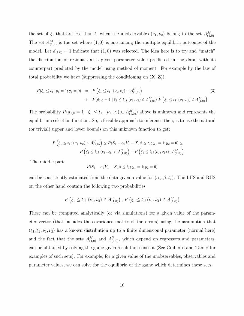
the set of ξ1 that are less than t1 when the unobservables (ν1, ν2) belong to the set AM(1,0).

The set AM(1,0) is the set where (1, 0) is one among the multiple equilibria outcomes of the

model. Let d(1,0) = 1 indicate that (1, 0) was selected. The idea here is to try and “match”

the distribution of residuals at a given parameter value predicted in the data, with its

counterpart predicted by the model using method of moment. For example by the law of

total probability we have (suppressing the conditioning on (X,Z)):

P (ξ1 ≤ t1; y1 = 1; y2 = 0) = P(ξ1 ≤ t1; (ν1, ν2) ∈ AU

(1,0)

)(3)

+ P (d1,0 = 1 | ξ1 ≤ t1; (ν1, ν2) ∈ AM(1,0)) P

(ξ1 ≤ t1; (ν1, ν2) ∈ AM

(1,0)

)The probability P (d1,0 = 1 | ξ1 ≤ t1; (ν1, ν2) ∈ AM(1,0)) above is unknown and represents the

equilibrium selection function. So, a feasible approach to inference then, is to use the natural

(or trivial) upper and lower bounds on this unknown function to get:

P(ξ1 ≤ t1; (ν1, ν2) ∈ AU

(1,0)

)≤ P (S1 + α1V1 −X1β ≤ t1; y1 = 1; y2 = 0) ≤

P(ξ1 ≤ t1; (ν1, ν2) ∈ AU

(1,0)

)+ P

(ξ1 ≤ t1; (ν1, ν2) ∈ AM

(1,0)

)The middle part

P (S1 − α1V1 −X1β ≤ t1; y1 = 1; y2 = 0)

can be consistently estimated from the data given a value for (α1, β, t1). The LHS and RHS

on the other hand contain the following two probabilities

P(ξ1 ≤ t1; (ν1, ν2) ∈ AU(1,0)

), P(ξ1 ≤ t1; (ν1, ν2) ∈ AM(1,0)

)These can be computed analytically (or via simulations) for a given value of the param-

eter vector (that includes the covariance matrix of the errors) using the assumption that

(ξ1, ξ2, ν1, ν2) has a known distribution up to a finite dimensional parameter (normal here)

and the fact that the sets AM(1,0) and AU(1,0), which depend on regressors and parameters,

can be obtained by solving the game given a solution concept (See Ciliberto and Tamer for

examples of such sets). For example, for a given value of the unobservables, observables and

parameter values, we can solve for the equilibria of the game which determines these sets.

10

Remark 2 We bound the distribution of the residuals as opposed to just the distribution

of S1 to allow some of the regressors to be endogenous. The conditioning sets in the LHS

(and RHS) depend on exogenous covariates only, and hence these probabilities can be easily

computed or simulated (for a given value of the parameters).

Similarly, the upper and lower bounds on the probability of the event (S2−α2V2−X2β ≤

t2, y1 = 0, y2 = 1) can similarly be calculated. In addition, in the two player entry game (δ’s

are negative) above with pure strategies, the events (1, 1) and (0, 0) are uniquely determined,

and so

P (S1 − α1V1 −X1β ≤ t1; S2 − α2V2 −X2β ≤ t2; y1 = 1; y2 = 1)

is equal to (moment equality)

P (ξ1 ≤ t1, ξ2 ≤ t2, ν1 ≥ −δ2 − γZ1, ν2 ≥ −δ1 − γZ2)

which can be easily calculated (via simulation for example). We also have:

P (y1 = 0, y2 = 0) = P (ν1 ≤ −γZ1, ν2 ≤ −γZ2)

The statistical moment inequality conditions implied by the model at the true parameters

are:

m1(1,0)(t1,Z; Σ) ≤ E

(1[S1 − α1V1 −X1β ≤ t1; y1 = 1; y2 = 0

])≤ m2

(1,0)(t1,Z; Σ)

m1(0,1)(t2,Z; Σ) ≤ E

(1[S2 − α2V2 −X2β ≤ t2; y1 = 0; y2 = 1

])≤ m1

(0,1)(t2,Z; Σ)

E(1[S1 − α1V1 −X1β ≤ t1;S2 − α2V2 −X2β ≤ t2; y1 = 1; y2 = 1

])= m(1,1)(t1, t2,Z; Σ)

E(1[y1 = 0; y2 = 0

])= m(0,0)(Z; Σ)

11

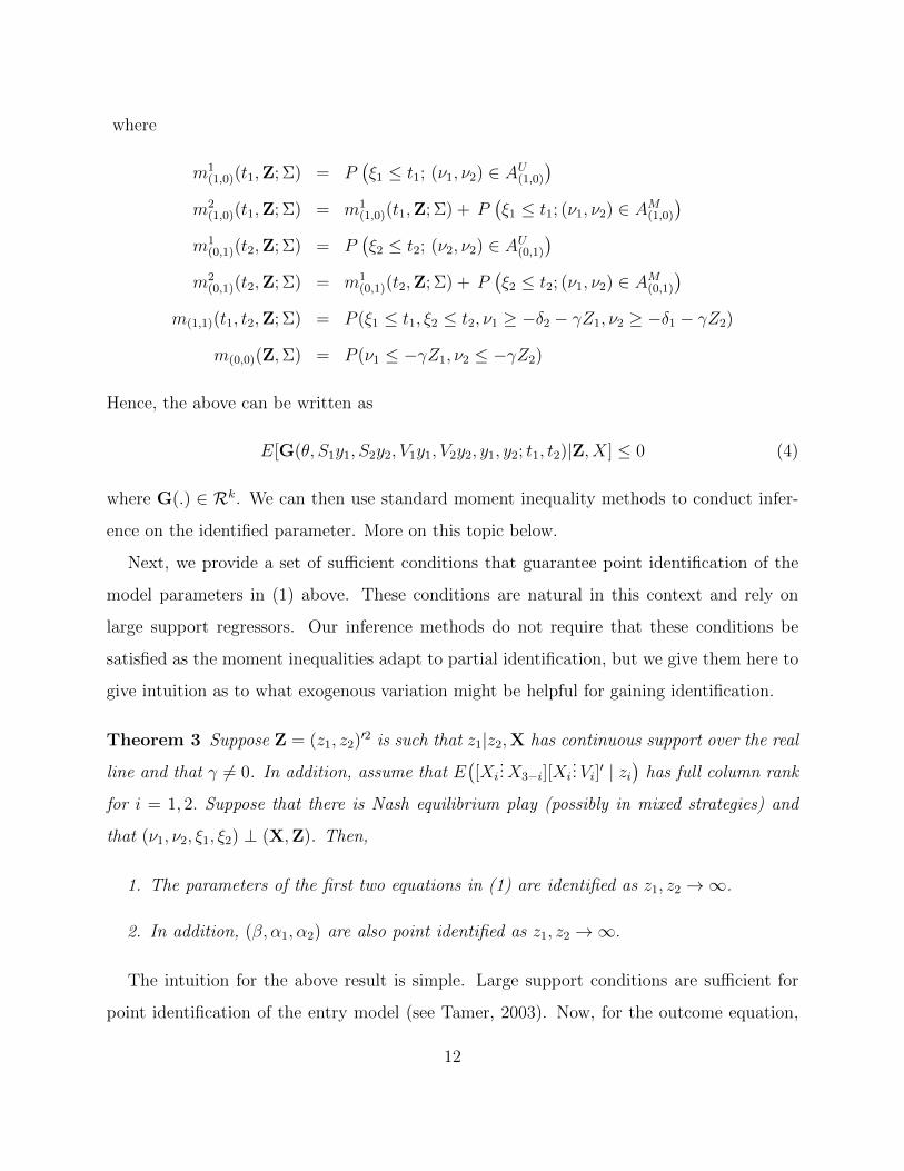
where

m1(1,0)(t1,Z; Σ) = P

(ξ1 ≤ t1; (ν1, ν2) ∈ AU(1,0)

)m2

(1,0)(t1,Z; Σ) = m1(1,0)(t1,Z; Σ) + P

(ξ1 ≤ t1; (ν1, ν2) ∈ AM(1,0)

)m1

(0,1)(t2,Z; Σ) = P(ξ2 ≤ t2; (ν2, ν2) ∈ AU(0,1)

)m2

(0,1)(t2,Z; Σ) = m1(0,1)(t2,Z; Σ) + P

(ξ2 ≤ t2; (ν1, ν2) ∈ AM(0,1)

)m(1,1)(t1, t2,Z; Σ) = P (ξ1 ≤ t1, ξ2 ≤ t2, ν1 ≥ −δ2 − γZ1, ν2 ≥ −δ1 − γZ2)

m(0,0)(Z,Σ) = P (ν1 ≤ −γZ1, ν2 ≤ −γZ2)

Hence, the above can be written as

E[G(θ, S1y1, S2y2, V1y1, V2y2, y1, y2; t1, t2)|Z, X] ≤ 0 (4)

where G(.) ∈ Rk. We can then use standard moment inequality methods to conduct infer-

ence on the identified parameter. More on this topic below.

Next, we provide a set of sufficient conditions that guarantee point identification of the

model parameters in (1) above. These conditions are natural in this context and rely on

large support regressors. Our inference methods do not require that these conditions be

satisfied as the moment inequalities adapt to partial identification, but we give them here to

give intuition as to what exogenous variation might be helpful for gaining identification.

Theorem 3 Suppose Z = (z1, z2)′2 is such that z1|z2,X has continuous support over the real

line and that γ 6= 0. In addition, assume that E([Xi

...X3−i][Xi...Vi]

′ | zi)

has full column rank

for i = 1, 2. Suppose that there is Nash equilibrium play (possibly in mixed strategies) and

that (ν1, ν2, ξ1, ξ2) ⊥ (X,Z). Then,

1. The parameters of the first two equations in (1) are identified as z1, z2 →∞.

2. In addition, (β, α1, α2) are also point identified as z1, z2 →∞.

The intuition for the above result is simple. Large support conditions are sufficient for

point identification of the entry model (see Tamer, 2003). Now, for the outcome equation,

12

we can do 2SLS at infinity as follows. For large values of z1 (large negative or positive values

depend on the sign of γ which can be learned fast by looking at whether large positive values

of z1 say correspond to higher likelihood of seeing a player 1 in the market) for example,

player 1 is in the market with probability 1. Hence, we can use X2 as an instrument for V1

and do 2sls on the first outcome equation conditional on the event that z1 → ∞. Driving

player 1 to enter with probability 1 eliminates the correlation between ξ1 and y1 = 1 which

allows us to use “standard methods” to estimate the first outcome equation. These methods

would be based on the moment condition

E[(X ′1, X′2)′ξ1|z1 →∞] = 0

Hence, what is needed for the identification of outcome equation 1 for example (arguments for

the second outcome equation are similar) is two excluded variables: a standard instrument

X2 and an excluded variable from the outcome equation, z1 in this case, that takes large

values and can influence the entry of player 1. Such a variable can be one that affects fixed

costs only, but not variable costs and can be exogenously moved. In the standard case, the

only needed condition is an instrument X2. So, to control for the first stage, we are required

to have another instrument that can take large values. Note that the identification results

in the Theorem above do NOT require that 1) the joint distribution of the unobservables be

known, but requires that those be independent of the exogenous regressors, and 2) that the

players play pure strategies (also here, the results in the Theorem do not require that the

sign of the ∆’s be known but we maintain here that the sign of these is strictly negative).

Without such large support conditions, it is unclear whether we get point identification

and hence it is crucial that any inference methods used is robust to failure of point identi-

fication. Basing our inference on the derived moment inequalities does not require that the

parameter is point identified. The confidence regions that these methods use are based on

inverting test statistics like the following ones.

So, under the null that θ = θ∗, we have

H0 : E[G(θ∗, S1y1, S2y2, V1y1, V2y2, y1, y2)|Z, X] ≤ 0 for all (X,Z, t1, t2)

13

HA : E[G(θ∗, S1y1, S2y2, V1y1, V2y2, y1, y2)|Z, X] > 0 for some (X,Z, t1, t2)

There are many ways to define a test statistic here. We just take a simple approach using

a test statistic that is equal to zero on the identified set, and otherwise is strictly positive.

The next Theorem states the test statistic formally.

Theorem 4 Suppose the above parametric assumptions in model (1) are maintained. In ad-

dition, assume that (X,Z) ⊥ (ξ1, ξ2, ν2, ν2) where the latter is normally distributed with mean

zero and covariance matrix Σ. Then given a large data set on (y1, y2, S1y1, V1y1, S2y2, V2y2,X,Z)

the true parameter vector θ = (δ1, δ2, α1, α2, β, γ,Σ) minimizes the nonnegative objective

function below to zero:

Q(θ) = 0 =

∫W (X,Z)‖G(θ, S1y1, S2y2, V1y1, V2y2, y1, y2)|Z, X]‖+dFX,Z (5)

for a strictly positive weight function (X,Z).

The above is a standard conditional moment inequality model where we employ discrete

valued variables in the conditioning set along with a finite (and small) set of t’s.7

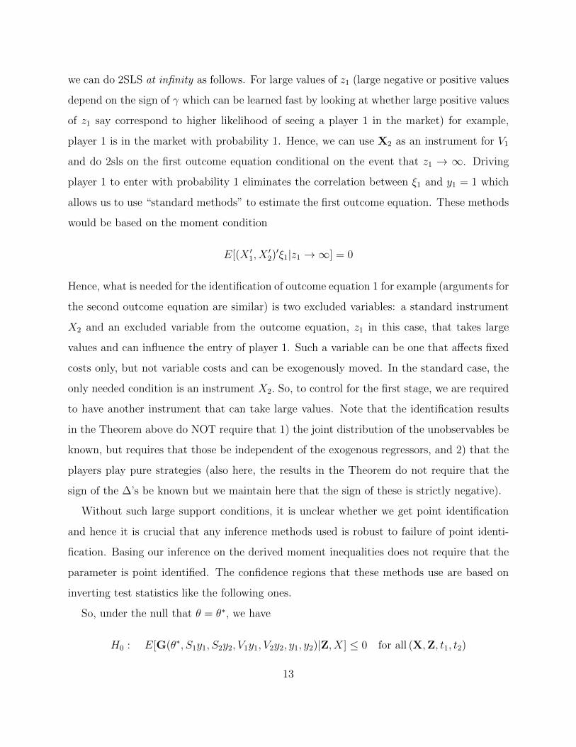
A Graphical Illustration of the Proposed Methodology. Figure 1 illustrates how

the methodology works. Between the origin and the point A, the CDF of the data predicted

residuals lies above the upper bound of the model predicted residuals which violates the

model under the null, hence the difference (squared) between the two is included in the

computation of the distance function. Between the points A and B, and the points C and

D, the CDF of the data predicted residuals lies between the lower and upper bounds, and

so the difference is not included in the computation of the distance. Between the point B

and C, the CDF of the data predicted residuals lies below the lower bound of the model

predicted residuals again violating the model under the null and so this difference (squared)

between the two is included in the computation of the distance function.

7It is possible to use recent advances in inference methods in moment inequality models with a continuumof moments, but these again will present severe computational difficulties especially in the empirical modelwe consider below. We detail in an online supplement the exact computational steps that we use to ensurewell behavior (and correct coverage) of our procedures.

14

Figure 1: Estimation MethodologyProbability

1

Upper Bound, H2 Lower Bound, H1

v ,

The CDF of the residuals is above The CDF of the residuals is below

the upper bound, so we take the the lower bound, so we take the

difference of the two PDFs to difference of the two CDFs to

construct the distance function construct the distance function

ξ

)( ξ

P

Clearly, the stylized model above provides intuition about the technical issues involved

but we now link this model to a clearer model of behavior where the decision to enter for

example (or to provide a product) is more explicitly linked to a usual economic condition of

profits. This entails specification of costs, demands, and a solution concept. This is done

next.

3 A Model of Entry and Price Competition

3.1 The Structural Model

The above considered a stylized model of entry and pricing that uses linear approximations

to various functions. It is simpler to explain the inference approach using such a model.

Here on the other hand, we build a fully structural model of entry and pricing and derive

formulas for entry thresholds directly from revenue and cost functions. The intuition for the

inference approach in Section 2 carries over to this model. To start with here, we consider

the case of duopoly interaction, where two firms must decide, simultaneously, whether to

serve a market and the prices they charge given their decision to enter.

15

The profits of firm 1 if this firm decides to enter is

π1 = (p1 − c (W1, η1))M · s1 (p,X,y, ξ)− F (Z1, ν1)

where

s1 (p,X,y, ξ) = s1 (p,X,y, ξ) y2 + s1 (p1, X1, ξ1) (1− y2)

is the share of firm 1 which depends on whether firm 2 is in the market, M is the market

size, c (W1, η1) is the constant marginal cost for firm 1, and F (Z1, ν1) is the fixed cost to

be paid by firm 1 to serve the market. Here, p = (p1, p2). A profit function for firm 2 is

specified in the same way.

In addition, we have the equilibrium first order conditions that determine shares and prices:(p1 − c (W1, η1)) ∂s1 (p,X,y, ξ) /∂p1 + s1 (p,X,y, ξ) = 0,(p2 − c (W2, η2)) ∂s2 (p,X,y, ξ) /∂p2 + s2 (p,X,y, ξ) = 0,

, (6)

These are the first order equilibrium conditions in the pricing game.

In this model, yj = 1 if firm j decides to enter a market, and yj = 0 otherwise where

j = 1, 2:

yj = 1 if and only if πj ≥ 0

There are six endogenous variables: p1, p2, S1, S2, y1, and y2. The observed exogenous

variables are M , W = (W1,W2), Z = (Z1, Z2), X = (X1, X2). So, putting these together, we

get the following system:

y1 = 1⇔ π1 = (p1 − c (W1, η1))M · s1 (p,X,y, ξ)− F (Z1, ν1) ≥ 0, Entry Conditions

y2 = 1⇔ π2 = (p2 − c (W2, η2))M · s2 (p,X,y, ξ)− F (Z2, ν2) ≥ 0,

S1 = s1 (p,X,y, ξ) , Demand

S2 = s2 (p,X,y, ξ) ,

(p1 − c (W1, η1)) ∂s1 (p,X,y, ξ) /∂p1 + s1 (p,X,y, ξ) = 0, Equilibrium Pricing

(p2 − c (W2, η2)) ∂s2 (p,X,y, ξ) /∂p2 + s2 (p,X,y, ξ) = 0,

(7)

16

The first two equations are entry conditions that require that in equilibrium a firm that

serves a market must be making non-negative profits. The third and fourth equations are

demand equations. The fifth and sixth equations are pricing first order conditions. An

equilibrium of the model occurs when firms make entry and pricing decisions such that all

the six equations are satisfied. The unobservables that enter into the fixed costs are denoted

by νj, j = 1, 2. The unobservables that enter into the variable costs are denoted by ηj,

j = 1, 2 while the unobservables that enter into the demand equations are denoted by ξj,

j = 1, 2. This system of equations (7) might have multiple equilibria.

It is interesting to compare this system to the ones we studied in Section 2 above and

notice the added nonlinearities that are present. Even though the conceptual approach

is the same, the inference procedure for this system is more computationally demanding.

The model in (7) is more complex than the model (1) because one needs to solve for the

equilibrium of the full model, which has six (rather than just four) endogenous variables. On

the other hand, one only had to solve for the equilibrium of the entry game in the model

(1). The methodology presented in Section (2) can be used to estimate model (7), but now

there are two unobservables for each firm over which to integrate (the marginal cost and the

demand unobservables).

To understand how the model relates to previous work, observe that if we were to estimate

a reduced form version of the first two equations of the system (7), then that would be akin

to the entry game literature (Bresnahan and Reiss, 1990, 1991; Berry, 1992; Mazzeo, 2002;

Seim, 2006; Ciliberto and Tamer, 2009). If we were to estimate the third to sixth equation

in the system (7), then that would be akin to the demand-supply literature (Bresnahan,

1987; Berry, 1994; Berry, Levinsohn, and Pakes, 1995), depending on the specification of

the demand system. So, here we join these two literatures together, while allowing the

unobservables of the six equations to be correlated with each other. This is important as

with this kind of model, we are able to have a richer picture when conducting policy such

as responses to a particular merger. This model would allow for market structure to adjust

17

and hence allow for example for exit/entry.

3.2 Parametrizing the model

To parametrize the various functions above, we follow Bresnahan (1987) and Berry, Levin-

sohn, and Pakes (1995), where the unit marginal cost can be written as:

ln c (Wj, ηj) = ϕjWj + ηj. (8)

Also, and similarly to entry game literature mentioned above, the fixed costs are

lnF (Zj, νj) = γjZj + νj. (9)

We will study how the results change as we allow for more heterogeneity among firms,

and thus we will have specifications where ϕj = ϕ and γj = γ for all j and then we will relax

these restrictions.

The demand is derived from a discrete choice model (Bresnahan, 1987; Berry, 1994; Berry,

Levinsohn, and Pakes, 1995). More specifically, we consider the nested logit model, which is

discussed at length in (Berry (1994)).

In the two goods world that we are considering in this Section, consumers choose among

the inside goods j = 1, 2 or choose neither one, and we will say in that case that they choose

the outside good, indexed with j = 0. The mean utility from the outside good (not traveling

or another form of transportation) is normalized to zero. There are two groups of goods,

one that includes all the flight options, and one that includes the decision of not flying.

The utility of consumer i from consuming j is

uij = X ′jβ + αpj + ξj + υig + (1− σ) εij, (10)

ui0 = εi0,

where Xj is a vector of product characteristics, pj is the price, (β, α) are the taste param-

eters, and ξj are product characteristics unobserved to the econometrician.

The term υig + (1 − σ)εij represents the individual specific unobservables. The term υig

is common for consumer i across all products that belong to group g. We maintain here

18

that the individual specific unobservables follow the distributional assumption that generate

the nested logit model (Cardell, 1991). The parameter, σ ∈ [0, 1], governs the substitution

patterns between the airline travel nest and the outside good. If σ = 0 then this is the logit

model. We consider the logit model in the Monte Carlo exercise presented in Appendix C.

The proportion of consumers who choose to fly is then

D(1−σ)

1 +D(1−σ)

where

D =J∑j=1

e(X′jβ+αpj+ξj)/(1−σ).

Recall that in this section, J = 2. In the empirical analysis, J will vary by market, and

will take values from 1 to 6.

The probability of a consumer choosing product j, conditional on purchasing a product

from the air travel nest, is

sj/g =e(X

′jβr+αpj+ξj)/(1−σ)

D(11)

Product j’s market share is

sj(X,p, ξ, βr, α, σ) =e(X

′jβ+αpj+ξj)/(1−σ)

D

D(1−σ)

1 +D(1−σ).(12)

Let E ≡ (y1, .., yj, .., yK) : yj = 1 or yj = 0,∀1 ≤ j ≤ K denote the set of possible mar-

ket structures. This set contains 2K elements and let e ∈ E be an element or a market

structure. For example, in the model above where K = 2, the set of possible market

structures is E = (0, 0) , (0, 1) , (1, 0) , (1, 1). Let Xe, pe, and ξe denote the matrices of,

respectively, the exogenous variables, prices, and unobservable firm characteristics when the

market structure is e.

Suppose, for sake of simplicity and just for the next few paragraphs, that σ = 0, so that

the demand is given by the standard logit model. When both firms are in the market, we

have:

19

sj(β, α,X(1,1),p(1,1), ξ(1,1)

)=exp(X ′jβ + αpj + ξj)

D

where D =∑

j∈J exp(X′jβ +αpj + ξj) and J = 1, 2 indicates the products in the market.8

Under the maintained distributional assumptions on ε, we can write the following rela-

tionship:

ln sj (β, α,Xe,pe, ξe)− ln s0 (β, α,Xe,pe, ξe) = Xjβ + αpj + ξj, (13)

The markup is then equal to (Berry (1994)):

bj (Xe,pe, ξe) =1

α [1− sj (β, α,Xe,pe, ξe)].

If we let σ = 0 free, then, under the maintained distributional assumptions, we can write

the following relationship:

ln sj (β, α,Xe,pe, ξe)− ln s0 (β, α,Xe,pe, ξe) = Xjβ + αpj + σ ln sj/g + ξj, (14)

where sj/g is defined in Equation 11.

Finally, the unobservables have a joint normal distribution,

(ν1, ν2, ξ1, ξ2, η1, η2) ∼ N (0,Σ) , (15)

where Σ is the variance-covariance matrix to be estimated. As discussed above, the off-

diagonal terms pick up the correlation between the unobservables is the source of the selec-

tivity bias in the model.

In this model, the variances of all the unobservables, in particular of the fixed costs that

enter in the entry equations, are identified. This is different from previous work in the

entry literature, where the variance of one or all firms had to be normalized to 1. Here,

the scale of the observable component of the fixed costs is tied down by the estimates of

the variable profits, which are derived from the demand and supply equations. Again, the

moment inequality based approach does not rely on parameter being point identified.

8So, for example, when only one firm is in the market, say firm j = 1, then the share equation forsj(β, α,X(1,0),p(1,0), ξ(1,0)

)is the same as above, except that D = exp(X ′1β + αp1 + ξ1).

20

3.3 Simulation Algorithm

To estimate the parameters of the model we need to predict market structure and derive

distributions of demand and supply unobservables to construct the distance function. This

requires the evaluation of a large multidimensional integral, therefore we have constructed

an estimation routine that relies heavily on simulation. We solve directly for all equilibria

at each iteration in the estimation routine.

The simulation algorithm is presented for the case when there are K potential entrants.

We rewrite the model of price and entry competition using the parameterizations above.

yj = 1⇔ πj ≡ (pj − exp (ϕWj + ηj))Msj (Xe,pe, ξe)− exp (γZj + νj) ≥ 0,

ln sj (β, α,Xe,pe, ξe)− ln s0 (β, α,Xe,pe, ξe) = X ′jβ + αpj + ξj

ln [pj − bj (Xe,pe, ξe)] = ϕWj + ηj,

, (16)

for j = 1, ..., K and e ∈ E.

We now explain the details of the simulation algorithm that we use.

First, set the candidate parameter value to be Θ0 = (α0, β0, ϕ0, γ0,Σ0) . Then, we take

ns pseudo-random independent draws from the a 3 × |K|-variate joint normal standard

distribution, where |K| is the cardinality of K. Let r = 1, ..., ns index pseudo-random

draws. These draws remain unchanged during the minimization. Next, the algorithm uses

three steps that we describe below.

1. We first construct the probability distributions for the residuals, which are estimated

non-parametrically at each parameter iteration. The steps here do not involve any

simulations.

(a) Take a market structure e ∈ E.

(b) If the market structure in market m is equal to e, use α0, β0, ϕ0 to compute the

demand and first order condition residuals ξej and ηej . These can be done easily

using (16) above.

21

(c) Repeat (b) above for all markets, and then construct Pr(ξe, ηe | X,W,Z), which

are joint probability distributions of ξe, ηeconditional on the values taken by the

control variables.9

(d) Repeat the steps 1(b) and 1(c) above for all e ∈ E.

2. Next, we construct the probability distributions for the lower and upper bound of the

“simulated errors”. For each market we have:

(a) We simulate random vectors of unobservables (νr, ξr, ηr) from a multivariate

normal density with a given covariance matrix.

(b) For each potential market structure e of the 2|K| − 1 possible ones (excluded the

one where no firm enters), we solve the subsystem of the |e| demand equations

and the |e| first order conditions in (16) for the equilibrium prices per and shares

ser, where |e| is the cardinality of the set of entrants e.10

(c) We compute 2|K| − 1 variable profits.

(d) We use the candidate parameter γ0 and the simulated error νr to compute 2|K|−1

fixed costs and total profits.

(e) We use the total profits to determine which of the 2|K| market structures are

predicted as equilibria of the full model. If there is a unique equilibrium, say

e∗, then we collect the simulated errors of the firms that are present in that

equilibrium, ξe∗r and ηe

∗r . In addition, we collect νe

∗r and include them in AUe∗ ,

which was defined in Section (2). If there are multiple equilibria, say e∗ and

e∗∗, then we collect the “simulated errors” of the firms that are present in those

equilibria, respectively(ξe∗r , η

e∗r

)and

(ξe∗∗r , ηe

∗∗r

). In addition, we collect νe

∗r and

νe∗∗r and include them, respectively, in AMe∗ and AMe∗∗ , which were also defined in

Section (2).

9Here, we use conditional CDFs evaluated at a grid. But, in principle, any parameter that obeys firstorder stochastic dominance can be used such as means and quantiles.

10For example, if we look at a monopoly of firm j (|e| = 1) then the demand Qj (pjr, Xjr, ξjr;β) is readilycomputed, and the monopoly price, pjr, as well.

22

(f) We repeat steps 2.a-2.e for all markets and simulations, and then we construct

Pr(ξer , η

er ; ν ∈ AMe |X,W,Z

)and Pr

(ξer , η

er ; ν ∈ AUe |X,W,Z

).

3. We construct the distance function (5) as in Section (2).

Comments on procedure above: The above is a modified minimum distance proce-

dure. In the absence of endogeneity and multiple equilibria, the above procedure compares

the distribution function of the data to the CDF predicted by the model at a given parameter

value. For example, in a linear model y = x′β + ε with ε ∼ N(0, 1), a similar procedure

compare the distribution of residuals P (y−x′β|x) to the standard normal CDF. Endogeneity

requires us to compare the distribution of residuals, and multiple equilibria leads to upper

and lower probabilities, and hence the modified version of the well known minimum distance

procedure. Many simplifications can be done to the above to ease the computational bur-

den. For example, though the inequalities hold conditionally on every value of the regressor

vector, they also hold at any level of aggregation of the regressors. So, this leads to fewer

inequalities, but simpler computations.

3.4 Estimation: Practical Matters

The estimation mainly consists of minimizing the distance function given by Equation 5,

which is derived from the inequality moments that are constructed as explained in Section 2.

There are two main practical differences between the empirical analysis that follows and the

theoretical model in Section 2.11 First, the number of firms, and thus moments, is larger.

We will have up to six potential entrants, while in Section 2 there were only two. Second,

the number and identity of potential entrants will vary by market, which means that the set

of moments varies by market as well.

In addition to the moments constructed in Section 2, we will also use the moment in-

equality conditions from CT. The moments from CT ”match” the predicted and observed

market structure, and help the estimation, but are not necessary. In practice, we will choose

11We discuss other, less crucial, differences at length in Appendix A.

23

paramaters that minimize the sum of the value of the distance function given by Equation

5 and of the value of the distance function given by Equation 11 in CT.

We use the following variance-covariance matrix, where we do not estimate σ2ν and restrict

it to be equal to the value found in the GMM estimation.

Σm =

σ2ξ · IKm σξη · IKm σξν · IKm

σξη · IKm σ2η · IKm σην · IKm

σξν · IKm σην · IKm σ2ν · IKm

.Thus, we assume that the correlation is only among the unobservables of a firm (within-

firm correlation), and not between the unobservables of the Km firms (between-firm corre-

lation). This specification also restricts the correlations to be the same for each firm. This

specification clearly reduces the parameters to be estimated to just five.

4 Data and Industry Description

We apply our methods to data from the airline industry. This industry is particularly in-

teresting in our setting for two main reasons. First, there is considerable variation in prices

and market structure across markets and across carriers, which we expect to be associated

with self-selection of carriers into markets. Second, this is an industry where the study of

market structure and market power are particularly meaningful because there have been

several recent changes in the number and identity of the competitors, with recent mergers

among the largest carriers (Delta with Northwest, United with Continental, and American

with USAir). Our methods allow us to examine within the context of our model the impli-

cations of mergers on equilibrium prices and also on market structure. Below, we start with

an examination of our data, and then we provide our estimates.

4.1 Market and Carrier Definition

Data. We use data from several sources to construct a cross-sectional dataset, where the

basic unit of observation is an airline in a market (a market-carrier). The main datasets

are the second quarter of 2012’s Airline Origin and Destination Survey (DB1B) and of the

24

T-100 Domestic Segment Dataset, the Aviation Support Tables, available from the DOT’s

National Transportation Library. We also use the US Census for the demographic data.12

We define a market as a unidirectional trip between two airports, irrespective of interme-

diate transfer points. The dataset includes the markets between the top 100 US Metropolitan

Statistical Areas ranked by their population. We include markets that are temporarily not

served by any carrier, which are the markets where the number of observed entrants is equal

to zero. There are 6, 322 unidirectional markets, and each one is denoted by m = 1, ...,M .

There are six carriers in the dataset: American, Delta, United, USAir, Southwest, and

a low cost type, denoted by LCC. The Low Cost Carrier type includes Alaska, JetBlue,

Frontier, AirTran, Allegiant, Spirit, Sun Country, Virgin. These firms rarely compete in

the same market. The subscript for carriers is j, j ∈ AA,DL,UA,UA,LCC. There are

20, 642 market-carrier observations for which we observe prices and shares. There are 172

markets that are not served by any firm.

We denote the number of potential entrants in market m as Km where |Km| ≤ 6. An

airline is considered a potential entrant if it is serving at least one market out of both of the

endpoint airports.13

Tables 1 and 2 present the summary statistics for the distribution of potential and actual

entrants in the airline markets. Table 1 shows that American Airlines enters in 48 percent

of the markets, although it is a potential entrant in 90 percent of markets. Southwest, on

the other hand, is a potential entrant in 38 percent of markets, and enters in 35 percent of

the time. So this already shows some interesting heterogeneity in the entry patterns across

airlines. Table 2 shows the distribution in the number of potential entrants, and we observe

that the large majority of markets have between four and six potential entrants, with less

than 1 percent having just one potential entrant.

For each firm in a market there are three endogenous variables: whether or not the firm is

in the market, the price that the firm charges in that market, and the number of passengers

12See Appendix B for a detailed discussion on the data cleaning and construction.13See Goolsbee and Syverson (2008) for an analogous definition. Variation in the identity and number of

potential entrants has been shown to help the identification of the parameters of the model (Ciliberto et al.,2010).

25

Table 1: Entry Moments

Actual Entry Potential Entry

AA 0.48 0.90DL 0.83 0.99LCC 0.26 0.78UA 0.66 0.99US 0.64 0.95WN 0.35 0.38

Table 2: Distribution of Potential Entrants

1 2 3 4 5 6

Fraction 0.08 1.11 5.16 18.11 42.87 32.68

transported. Following the notation used in the theoretical model, we indicate whether a

firm is active in a market as yjm = 1, and if it is not active as yjm = 0. For example, we set

yLCC = 1 if at least one of the low cost carriers is active.

Table 3 presents the summary statistics for the variables used in our empirical analysis.

For each variable we indicate in the last column whether the variable is used in the entry,

demand, and marginal cost equation.

The top panel of Table 3 reports the summary statistics for the ticket prices and passengers

transported in a quarter. For each airline that is actively serving the market we observe the

quarterly median ticket fare, pjm, and the total number of passengers transported in the

quarter, Qjm. The average value of the median ticket fare is 243.21 dollars and the average

number of passengers transported is 548.10.

Next we introduce the exogenous explanatory variables, explaining the rationale of our

choice and in which equation they enter.

Demand. Demand is here assumed to be a function of the number of non-stop routes that

an airline serves out of the origin airport, Nonstop Origin. We maintain that this variable is

a proxy of frequent flyer programs: the larger the share of nonstop markets that an airline

serves out of an airport, the easier is for a traveler to accumulate points, and the more

26

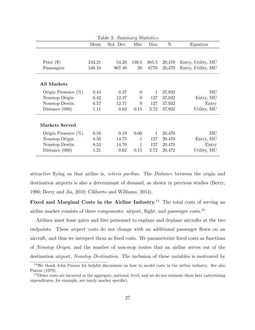
Table 3: Summary Statistics

Mean Std. Dev. Min Max N Equation

Price ($) 243.21 54.20 139.5 385.5 20,470 Entry, Utility, MCPassengers 548.10 907.40 20 6770 20,470 Entry, Utility, MC

All Markets

Origin Presence (%) 0.44 0.27 0 1 37,932 MCNonstop Origin 6.42 12.37 0 127 37,932 Entry, MCNonstop Destin. 6.57 12.71 0 127 37,932 EntryDistance (000) 1.11 0.63 0.15 2.72 37,932 Utility, MC

Markets Served

Origin Presence (%) 0.58 0.19 0.00 1 20.470 MCNonstop Origin 8.50 14.75 1 127 20.470 Entry, MCNonstop Destin. 8.53 14.70 1 127 20.470 EntryDistance (000) 1.21 0.62 0.15 2.72 20,472 Utility, MC

attractive flying on that airline is, ceteris paribus. The Distance between the origin and

destination airports is also a determinant of demand, as shown in previous studies (Berry,

1990; Berry and Jia, 2010; Ciliberto and Williams, 2014).

Fixed and Marginal Costs in the Airline Industry.14 The total costs of serving an

airline market consists of three components: airport, flight, and passenger costs.15

Airlines must lease gates and hire personnel to enplane and deplane aircrafts at the two

endpoints. These airport costs do not change with an additional passenger flown on an

aircraft, and thus we interpret them as fixed costs. We parameterize fixed costs as functions

of Nonstop Origin, and the number of non-stop routes that an airline serves out of the

destination airport, Nonstop Destination. The inclusion of these variables is motivated by

14We thank John Panzar for helpful discussions on how to model costs in the airline industry. See alsoPanzar (1979).

15Other costs are incurred at the aggregate, national, level, and we do not estimate them here (advertisingexpenditures, for example, are rarely market specific).

27

Brueckner and Spiller (1994) work on economies of density, whereby the larger the network

out of an airport, the lower is the market specific fixed cost faced by a firm because the same

gate and the same gate personnel can enplane and deplane many flights.

Next, a particular flight’s costs also enter the marginal cost. This is because these costs

depend on the number of flights serving a market, on the size of the planes used, on the fuel

costs, and on the wages paid to the pilots and flight attendants. Even with the indivisible

nature aircraft capacity and the tendency to allocate these costs to the fixed component, we

think it is more helpful to separate these costs from the fixed component because we think

of these flight costs as a (possibly random) function of the number of passengers transported

in a quarter divided by the aircraft capacity. Under such interpretation, the flight costs are

variable in the number of passengers transported in a quarter.

Finally, the accounting unit costs of transporting a passenger are those associated with

issuing tickets, in-flight food and beverages, and insurance and other liability expenses.

These costs are very small when compared to the airport and flight specific costs.

Both the flight and passenger costs enter the economic opportunity cost of flying a pas-

senger. This is the highest profit that the airline could make off of an alternative trip that

uses the same seat on the same plane, possibly as part of a flight connecting two different

airports (Elzinga and Mills, 2009).

The economic marginal cost is not observable (Rosse, 1970; Bresnahan, 1989; Schmalensee,

1989). We parameterize it as a function of Origin Presence, which is defined as the ratio of

markets served by an airline out of an airport over the total number of markets served out

of that airport by at least one carrier. The idea is that the the larger the whole network, not

just the nonstop routes, the higher is the opportunity cost for the airline because the airline

has more alternative trips for which to use a particular seat. That is, the variable Origin

Presence affects the economic marginal cost, since it captures the alternative uses of a seat

on a plane out of the origin airport. Given our interpretation of flight costs, we also allow

the marginal cost to be a function of the non-stop distance, Distance, between two airports.

28

4.2 Identification

Identification of the Entry Equation. The fixed cost parameters in the entry equations

are identified if there is a variable that shifts the fixed cost of one firm without changing the

fixed costs of the competitors. This condition was also required to identify the parameters

in Ciliberto and Tamer (2009). The variables that are used in this paper are Nonstop Origin

and Nonstop Destination. A crucial source of identification is also the variation in the

identity and number of potential entrants across markets. Intuitively, when there is only one

potential entrant we are back to a single discrete choice model and the parameters of the

exogenous variables are point identified.

Identification of the Demand Equation. Several variables are omitted in the demand

estimation and enter in ξ1 and ξ2. For example, we do not include frequency of flights or

whether an airline provides connecting or nonstop service between two airports. As men-

tioned before, quality of airline service is also omitted. Because these variables are strategic

choices of the airlines, their omission could bias the estimation of the price coefficient. The

parameters of the demand functions are identified because, in addition to the variable Non-

stop Origin, there are variables that affect prices through the marginal cost or through

changes to the demand of the other goods as in Bresnahan (1987) and Berry, Levinsohn, and

Pakes (1995). In our context, these are the Nonstop Origin of the competitors. In addition,

we maintain that after controlling for Nonstop Origin, the variables Origin Presence and,

especially, Nonstop Destination enter the fixed cost and marginal cost equations, but are

excluded from the demand equation.

16

4.3 Self-Selection in Airline Markets: Some Preliminary Evidence

The middle and bottom panels of Table 3 report the summary statistics for the exogenous

explanatory variables. The middle panel computes the statistics on the whole sample, while

16We have also looked at specifications where we included the variable Origin Presence in the demandestimation. We found that Origin Presence was neither economically nor statistically strongly significantwhen Nonstop Origin was also included.

29

the bottom panel computes the statistics only in the markets that are served by at least one

airline. We compare these statistics later on in the paper.17

The mean value of Origin Presence is 0.44 across all markets, but it is up to 0.58 in

markets that are actually served. This implies that firms are more likely to enter in markets

where they have a stronger airport presence, and face a stronger demand ceteris paribus.

The mean value of Nonstop Origin is 6.42 in all markets, and 8.50 in markets that were

actively served. This evidence suggests that firms self-select into markets out of airports

from where they serve a larger number nonstop markets. This is consistent with the notion

that fixed cost decline with economies of density. The magnitudes are analogous for Nonstop

Destination.

The mean value of Distance is 1.11, which implies that most market are long-distance. We

do not find that the market distance has a different distribution in market that are served

and the full sample.

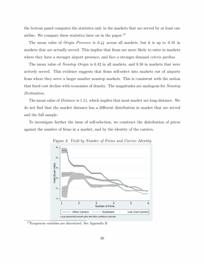
To investigate further the issue of self-selection, we construct the distribution of prices

against the number of firms in a market, and by the identity of the carriers.

Figure 2: Yield by Number of Firms and Carrier Identity

.1.2

.3.4

.5.6

Yie

ld (

$ p

er

mile

)

1 2 3 4 5 6Number of Firms

Other Carriers Southwest Low Cost Carriers

Local polynomial smooth plots with 95% confidence intervals

17Exogenous variables are discretized. See Appendix B

30

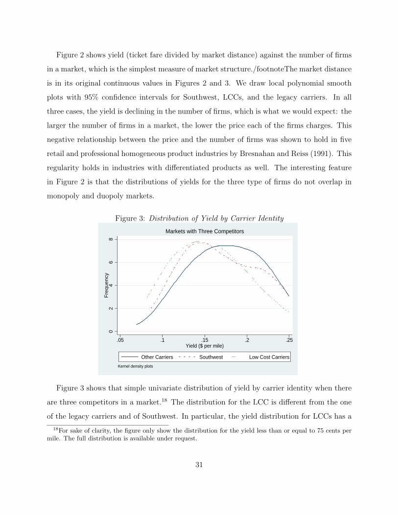
Figure 2 shows yield (ticket fare divided by market distance) against the number of firms

in a market, which is the simplest measure of market structure./footnoteThe market distance

is in its original continuous values in Figures 2 and 3. We draw local polynomial smooth

plots with 95% confidence intervals for Southwest, LCCs, and the legacy carriers. In all

three cases, the yield is declining in the number of firms, which is what we would expect: the

larger the number of firms in a market, the lower the price each of the firms charges. This

negative relationship between the price and the number of firms was shown to hold in five

retail and professional homogeneous product industries by Bresnahan and Reiss (1991). This

regularity holds in industries with differentiated products as well. The interesting feature

in Figure 2 is that the distributions of yields for the three type of firms do not overlap in

monopoly and duopoly markets.

Figure 3: Distribution of Yield by Carrier Identity

02

46

8F

req

ue

ncy

.05 .1 .15 .2 .25Yield ($ per mile)

Other Carriers Southwest Low Cost Carriers

Kernel density plots

Markets with Three Competitors

Figure 3 shows that simple univariate distribution of yield by carrier identity when there

are three competitors in a market.18 The distribution for the LCC is different from the one

of the legacy carriers and of Southwest. In particular, the yield distribution for LCCs has a

18For sake of clarity, the figure only show the distribution for the yield less than or equal to 75 cents permile. The full distribution is available under request.

31

median of 15.9 cents per mile while the yield distribution for the legacy carriers (American,

Delta, USAir, United) has a median of 22.3 cents per mile. The full distribution of the yield

by type of carrier is presented in Table 4.

Table 4: Distribution of Yield (Percentiles)

Min 10 25 50 75 90 Max

Legacy 0.059 0.120 0.153 0.223 0.342 0.515 2.205Southwest 0.066 0.111 0.133 0.190 0.289 0.443 1.706LCC 0.055 0.101 0.122 0.159 0.220 0.590 1.333

5 Results

We organize the discussion of the results in two steps. First, we present the results when we

estimate demand and supply using the standard GMM method. We present two specifica-

tions that differ by the degrees of heterogeneity in the marginal and cost functions. Then,

we present the results when we use the methodology that accounts for firms’ entry decisions,

and we again allow for different degrees of heterogeneity in the specification our model.

5.1 Results with Exogenous Market Structure

Column 1 of Table 5 shows the results from GMM estimation of a model where the inverted

demand is given by a nested logit regression, as in Equation 14, and where we set ϕj = ϕ

and γj = γ in Equations 8 and 9.

All the results are as expected and resemble those in previous work, for example Berry

and Jia (2010) and Ciliberto and Williams (2014). Starting from the demand estimates, we

find the price coefficient to be negative and σ, the nesting parameter, to be between 0 and 1.

The mean elasticity equals -5.978, the mean marginal cost is equal to 203.963 and the mean

markup is equal to 39.249. A larger presence at the origin airport is associated with more

demand as in (Berry, 1990), and longer route distance is associated with stronger demand

32

as well. The marginal cost estimates show that the marginal cost is increasing in distance,

and increasing in the number of nonstop service flights out of an airport.

Column 2 of Table 5 shows the results from GMM estimation of a model where more

flexible heterogeneity is allowed in the marginal cost equation. In particular, in Equations

8 we allow ϕj to be different for LCCs and Southwest. The results on the demand side

are largely unchanged. The results on the marginal cost side are not surprising, but still

quite interesting. The legacy carriers have a mean marginal cost of 206.013, while LCCs and

Southwest have considerably lower marginal costs. The mean of the marginal cost of LCC

is 189.943, which is 15 percent smaller than the legacy mean marginal cost. The mean of

the marginal cost of WN is 166.687, which is more than 20 percent smaller than the legacy

mean marginal cost. All the markups are approximately the same, with a mean equal to

approximately 42. We discuss further the markups in Table 10.

5.2 Results with Endogenous Market Structure

In order to present the results when we control for self-selection of firms into markets,

we report superset confidence regions that cover the true parameters with a pre-specified

probability. In Table 6, we report the cube that contains the confidence region that is

defined as the set that contains the parameters that cannot be rejected as the truth with at

least 95% probability. This is the approach that was used in CT.

Column 1 of Table 6 shows the results when we use the methodology developed in Section

2 and the inverted demand is given by a nested logit regression, as in Equation 14, and where

8 and 9 we set ϕj = ϕ and γj = γ. Thus, this model shows results that we can directly

compare with those in Column 1 of Table 5.

We estimate the coefficient of price to be included in [-0.016, -0.012], which is 25 percent

larger, in absolute magnitude, than the coefficient we estimated in Column 1 of Table 5.

This is the first of our main findings, and it implies that the model that does not account

for endogenous market structure gives bias estimates of price elasticity and therefore market

power. We take up this issue in more detail in the next section where we compare the implied

33

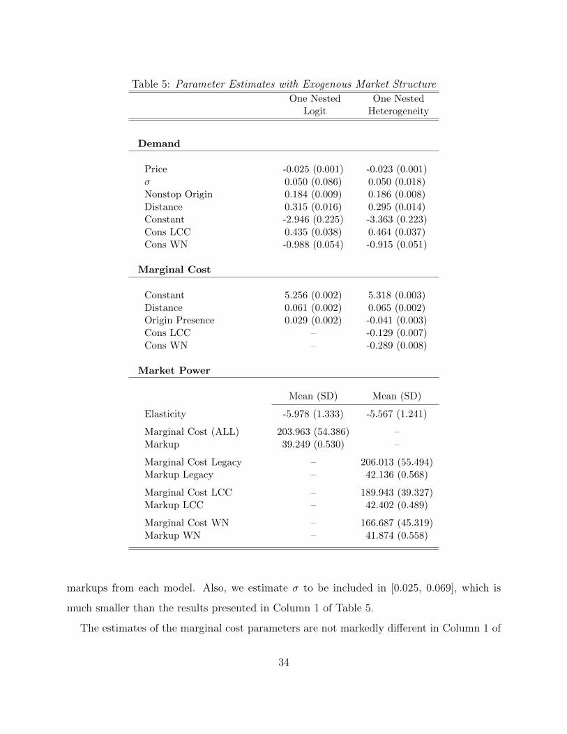
Table 5: Parameter Estimates with Exogenous Market Structure

One Nested One NestedLogit Heterogeneity

Demand

Price -0.025 (0.001) -0.023 (0.001)σ 0.050 (0.086) 0.050 (0.018)Nonstop Origin 0.184 (0.009) 0.186 (0.008)Distance 0.315 (0.016) 0.295 (0.014)Constant -2.946 (0.225) -3.363 (0.223)Cons LCC 0.435 (0.038) 0.464 (0.037)Cons WN -0.988 (0.054) -0.915 (0.051)

Marginal Cost

Constant 5.256 (0.002) 5.318 (0.003)Distance 0.061 (0.002) 0.065 (0.002)Origin Presence 0.029 (0.002) -0.041 (0.003)Cons LCC – -0.129 (0.007)Cons WN – -0.289 (0.008)

Market Power

Mean (SD) Mean (SD)

Elasticity -5.978 (1.333) -5.567 (1.241)

Marginal Cost (ALL) 203.963 (54.386) –Markup 39.249 (0.530) –

Marginal Cost Legacy – 206.013 (55.494)Markup Legacy – 42.136 (0.568)

Marginal Cost LCC – 189.943 (39.327)Markup LCC – 42.402 (0.489)

Marginal Cost WN – 166.687 (45.319)Markup WN – 41.874 (0.558)

markups from each model. Also, we estimate σ to be included in [0.025, 0.069], which is

much smaller than the results presented in Column 1 of Table 5.

The estimates of the marginal cost parameters are not markedly different in Column 1 of

34

Table 6 from the ones in Column 1 of Table 5. The constant is included in [4.092, 4.695], the

coefficients of distance and nonstop routes in, respectively, [0.014, 0.039] and [0.031, 0.078].

Next, we show the results for the estimates of the fixed cost equations. Clearly, these are

not comparable to the results from the previous model where market structure is assumed

to be exogenous. Column 1 of Table 6 shows the constant in the fixed cost equation to be

included in [10.948, 11.891], and the variables Nonstop Origin and Nonstop Destination to

be negative, as one would expect if there were economies of density.

Finally, we investigate the estimation results for the variance-covariance matrix. The

variances are precisely estimated, with the demand variance being included in [2.924,3.059]

and the the variance of the fixed costs to be in [1.336,1.500]. The correlations are clearly of

crucial interest for our analysis. In Column 1 the correlation between the demand and the

marginal cost unobservables is not precisely estimated; in Column 2 it is, and is included

in [-0.542,-0.354]. This implies that unobservables that would, ceteris paribus, increase

the demand for a given good, are negatively correlated with those that would increase the

marginal cost. This suggests that firms that are more likely to serve a larger market share

are also those that are more likely to face lower marginal costs.

The unobservables of the demand are also negatively correlated with those in the fixed

costs. Which means that firms that are more likely to face a higher demand are also those

that are facing lower fixed costs, ceteris paribus. This indicates that self-selection occurs,

in the sense that firms that are more likely to be in a market because they face lower fixed

costs are also the firms that are more likely to offer higher quality products.

Finally, there is some evidence that the unobservables in the fixed and marginal costs are

positively correlated, though this relationship is not statistically significant in Column 2. A

positive correlation indicates that firms that have the lowest unobservable components of the

fixed costs are also the ones that have the lowest unobservable components of the marginal

costs. We interpret this as further evidence of self-selection into markets.

The results in Column 2 of Table 6 are overall similar to the ones in Column 1. The main

differences concern the estimate of the utility constant, which now is much more precise.

35

The estimates for the constant terms of the LCC and WN are analogous to those in Table

5.

We also estimate heterogeneity among firms in the cost functions. We find that Southwest

has lower fixed costs than the legacy carriers. We do not find a statistically significant

difference between the marginal costs of the legacy carriers and Southwest, although we find

that LCCs have both higher marginal costs and fixed costs, an opposite finding to the model

with exogenous market structure. The variance covariance estimates are again not precisely

estimated.

5.3 Analysis of Fit

Next, we discuss few ways to understand how our model fits the data, and possible avenues

of research to improve the fit. We also discuss the economic significance of the estimates

in Table 6 by looking at the markups and the monetary magnitude of the fixed costs. The

starting point is to look at the fit in terms of market structure, which we do in two ways.

First, we look at the fit in terms of the individual firms. Then, we look at the fit in terms of

the number of firms.

Table 7 shows that we observe American in 48.10 percent of the markets in our dataset.

Our estimates in Table 6 imply that we predict American to be in [53.96 55.53] percent of

the markets, as shown in Column 2 of Table 7. To explore further this fit, we construct an

additional measure, which is presented in Column 3 of Table 7, and which is based on the

comparison of the percentage of times that American is observed in the data and is predicted

to be in by the model, and that American is not observed in the data and is not predicted

by the model. This exercise is analogous to the one that is done when studying the fit in

a probit estimation, where a cross tab of 0/1 between observed and predicted outcomes is

used. In this context, we find that our estimates fit approximately 60 percent of the 0/1

(entry/exit) outcomes for American. The results are similar for the other firms. The fit is

excellent for Southwest, which might be explained by the fact that we allow for heterogeneity

in their cost functions. However, the fit is the worst for LCCs, which may be attributed to

36

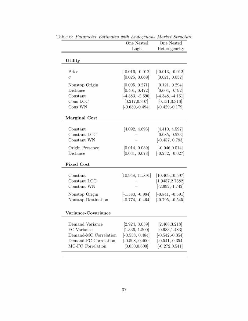
Table 6: Parameter Estimates with Endogenous Market Structure

One Nested One NestedLogit Heterogeneity

Utility

Price [-0.016, -0.012] [-0.013, -0.012]σ [0.025, 0.069] [0.021, 0.052]

Nonstop Origin [0.095, 0.271] [0.121, 0.294]Distance [0.401, 0.472] [0.604, 0.792]Constant [-4.383, -2.690] [-4.348, -4.161]Cons LCC [0.217,0.307] [0.151,0.316]Cons WN [-0.630,-0.494] [-0.429,-0.179]

Marginal Cost

Constant [4.092, 4.695] [4.410, 4.597]Constant LCC – [0.085, 0.523]Constant WN – [-0.457, 0.793]

Origin Presence [0.014, 0.039] [-0.046,0.014]Distance [0.031, 0.078] [-0.232, -0.027]

Fixed Cost

Constant [10.948, 11.891] [10.409,10.597]Constant LCC – [1.9457,2.7582]Constant WN – [-2.992,-1.742]

Nonstop Origin [-1.580, -0.984] [-0.841, -0.591]Nonstop Destination [-0.774, -0.464] [-0.795, -0.545]

Variance-Covariance

Demand Variance [2.924, 3.059] [2.468,3.218]FC Variance [1.336, 1.500] [0.983,1.483]Demand-MC Correlation [-0.558, 0.484] [-0.542,-0.354]Demand-FC Correlation [-0.598,-0.400] [-0.541,-0.354]MC-FC Correlation [0.030,0.600] [-0.272,0.541]

37

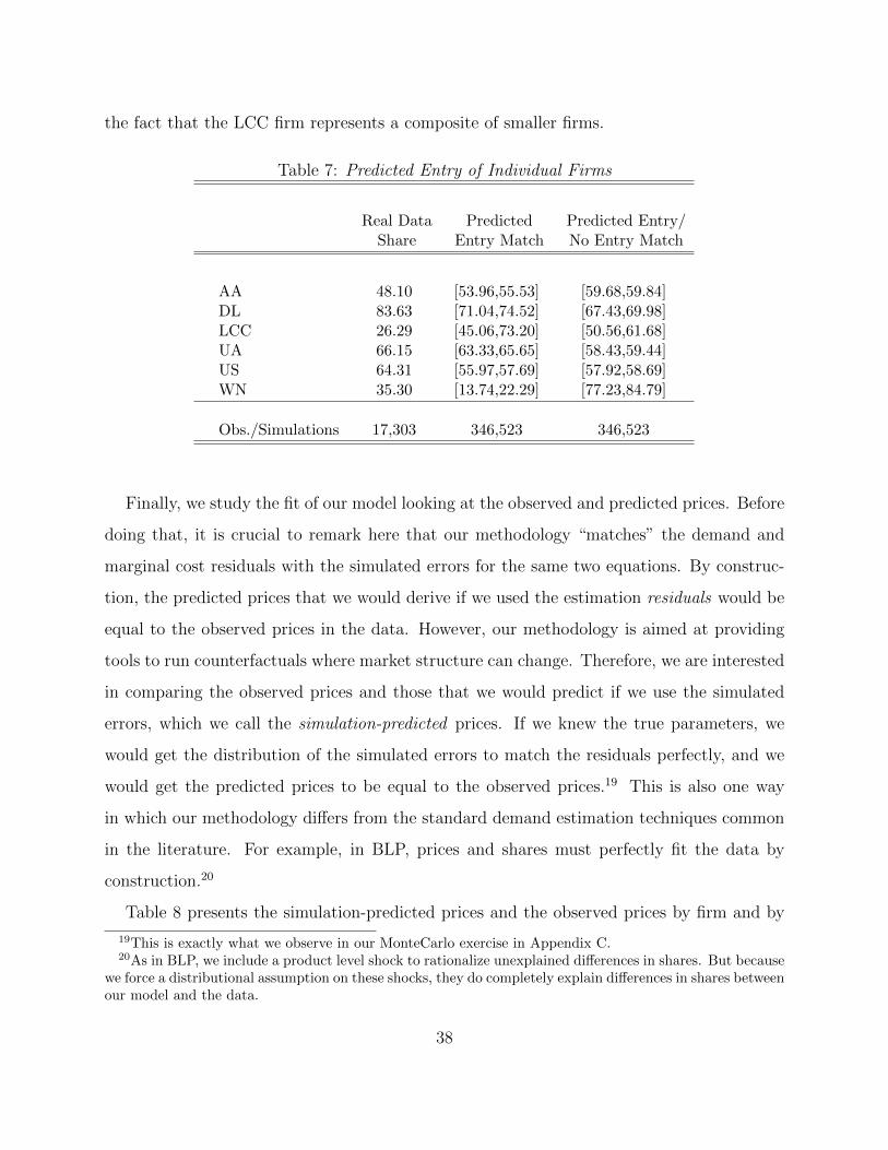
the fact that the LCC firm represents a composite of smaller firms.

Table 7: Predicted Entry of Individual Firms

Real Data Predicted Predicted Entry/Share Entry Match No Entry Match

AA 48.10 [53.96,55.53] [59.68,59.84]DL 83.63 [71.04,74.52] [67.43,69.98]LCC 26.29 [45.06,73.20] [50.56,61.68]UA 66.15 [63.33,65.65] [58.43,59.44]US 64.31 [55.97,57.69] [57.92,58.69]WN 35.30 [13.74,22.29] [77.23,84.79]

Obs./Simulations 17,303 346,523 346,523

Finally, we study the fit of our model looking at the observed and predicted prices. Before

doing that, it is crucial to remark here that our methodology “matches” the demand and

marginal cost residuals with the simulated errors for the same two equations. By construc-

tion, the predicted prices that we would derive if we used the estimation residuals would be

equal to the observed prices in the data. However, our methodology is aimed at providing

tools to run counterfactuals where market structure can change. Therefore, we are interested

in comparing the observed prices and those that we would predict if we use the simulated

errors, which we call the simulation-predicted prices. If we knew the true parameters, we

would get the distribution of the simulated errors to match the residuals perfectly, and we

would get the predicted prices to be equal to the observed prices.19 This is also one way

in which our methodology differs from the standard demand estimation techniques common

in the literature. For example, in BLP, prices and shares must perfectly fit the data by

construction.20

Table 8 presents the simulation-predicted prices and the observed prices by firm and by

19This is exactly what we observe in our MonteCarlo exercise in Appendix C.20As in BLP, we include a product level shock to rationalize unexplained differences in shares. But because

we force a distributional assumption on these shocks, they do completely explain differences in shares betweenour model and the data.

38

market structure. We observe that the fit is excellent in some instances, for example for Delta

and LCCs in most of the market structures, but the fit is not as good in other instances,

especially for American and United. This is likely due to many factors, including lack of

heterogeneity in both the utility function, as well as the cost functions. Because our method

does not force shares in the data to equal shares predicted in the model, it is hard to compare

our price fit to existing methods for demand estimation.

Table 8: Observed vs Prices Predicted with Simulated Errors, 1-3 Entrants

Monopoly Duopoly Three Firms

Data CMT Data CMT Data CMT

AA 297 [157, 181] 277 [158, 180] 256 [161, 183]DL 268 [155, 175] 237 [156, 175] 244 [159, 180]LCC 248 [144, 308] 214 [137, 271] 202 [140, 278]UA 260 [156, 175] 266 [155, 176] 251 [157, 178]US 245 [152, 167] 254 [153, 171] 268 [157, 178]WN 249 [165, 227] 224 [165, 224] 239 [168, 225]

Table 9: Observed vs Prices Predicted with Simulated Errors, 4-6 Entrants

Four Firms Five Firms Six Firms

Data CMT Data CMT Data CMT

AA 237 [162, 185] 237 [162, 188] 230 [163, 191]DL 237 [160, 184] 237 [162, 188] 234 [165, 194]LCC 199 [139, 277] 216 [141, 287] 211 [143, 301]UA 239 [159, 182] 236 [160, 186] 227 [162, 190]US 277 [160, 183] 280 [160, 187] 279 [163, 191]WN 234 [168, 225] 231 [169, 229] 229 [175, 240]

5.4 The Economics of Market Structure and Competition.

Next we now investigate how we can use the estimates in Table 6 to make inferences on

the economics of market structure and competition. We simulate our the model in order to

compute the markups, variable profits, and fixed costs. We compare these predictions to the

predictions from the model that took market structure as exogenous, except in the case of

fixed costs, where we have no estimates for the exogenous market structure model.

39

In Tables 10 and 11 we present the results, by methodology (GMM vs ours), and by market

structure. We observe that the markups we predict are consistently much larger than those

that one would estimate using GMM, suggesting that not controlling for self-selection of firms

into markets would lead to estimates of markups that are biased downward.21 This result

is driven by the differences in the price elasticities between the two models. As one would

expect given the markup result, the variable profits that we infer using our methodology are

also much larger than those that one would infer using GMM.22 We estimate the fixed costs

of active firms vary considerably. Mean fixed costs, for a given firm and market structure,

range from less than $100,000 per quarter, to more than $2 million per quarter.

Mean variable profits, and prices, are not monotonically decreasing in market structure.

This is due to self selection of firms, based on the marginal and fixed costs each firm faces

in each market and the mix of potential profits from all potential entrants. Because of this

self selection and the heterogeneity of firms, it is not clear that there is any systematic

relationship between market concentration and consumer and firm outcomes. This is an

important finding, as it suggest regressing HHI on some outcome measure may obscure the

actual economics of market structure and competition. A structural model, like the one we

present, is able to capture heterogeneity of firms across markets, and selection into markets,

in order to inform researchers about the effects of market concentration.

6 The Economics of Collusion and Mergers When Mar-

ket Structure is Endogenous

We present results from counterfactual exercises where we allow, separately, collusion be-

tween all of the legacy carriers, and a merger between two legacy firms, American and

US Airways. A typical question asked of anti-trust authorities when analyzing a potential

merger is whether prices would rise significantly after the merger. To do this, standard

21We explore this point in much more detail in the Appendix, where we conduct Monte Carlo simulationsand show numerically that market power is biased when demand and supply estimation does not control forendogenous selection of firms.

22The size of the variable profits are also driven by the fact that our model tends to over-predict demand.Computed variable profits would be much lower if we used shares from the data.

40

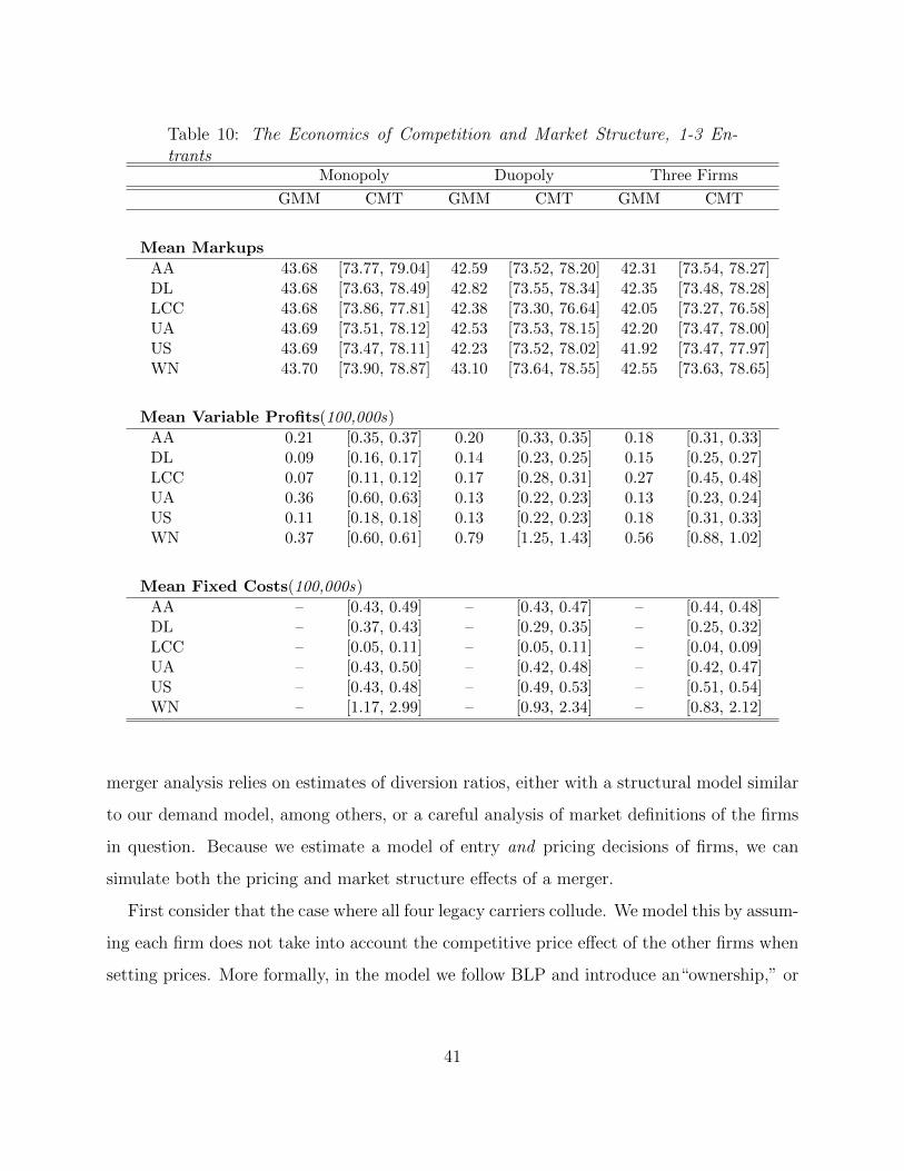
Table 10: The Economics of Competition and Market Structure, 1-3 En-trants

Monopoly Duopoly Three Firms

GMM CMT GMM CMT GMM CMT

Mean Markups

AA 43.68 [73.77, 79.04] 42.59 [73.52, 78.20] 42.31 [73.54, 78.27]DL 43.68 [73.63, 78.49] 42.82 [73.55, 78.34] 42.35 [73.48, 78.28]LCC 43.68 [73.86, 77.81] 42.38 [73.30, 76.64] 42.05 [73.27, 76.58]UA 43.69 [73.51, 78.12] 42.53 [73.53, 78.15] 42.20 [73.47, 78.00]US 43.69 [73.47, 78.11] 42.23 [73.52, 78.02] 41.92 [73.47, 77.97]WN 43.70 [73.90, 78.87] 43.10 [73.64, 78.55] 42.55 [73.63, 78.65]

Mean Variable Profits(100,000s)

AA 0.21 [0.35, 0.37] 0.20 [0.33, 0.35] 0.18 [0.31, 0.33]DL 0.09 [0.16, 0.17] 0.14 [0.23, 0.25] 0.15 [0.25, 0.27]LCC 0.07 [0.11, 0.12] 0.17 [0.28, 0.31] 0.27 [0.45, 0.48]UA 0.36 [0.60, 0.63] 0.13 [0.22, 0.23] 0.13 [0.23, 0.24]US 0.11 [0.18, 0.18] 0.13 [0.22, 0.23] 0.18 [0.31, 0.33]WN 0.37 [0.60, 0.61] 0.79 [1.25, 1.43] 0.56 [0.88, 1.02]

Mean Fixed Costs(100,000s)

AA – [0.43, 0.49] – [0.43, 0.47] – [0.44, 0.48]DL – [0.37, 0.43] – [0.29, 0.35] – [0.25, 0.32]LCC – [0.05, 0.11] – [0.05, 0.11] – [0.04, 0.09]UA – [0.43, 0.50] – [0.42, 0.48] – [0.42, 0.47]US – [0.43, 0.48] – [0.49, 0.53] – [0.51, 0.54]WN – [1.17, 2.99] – [0.93, 2.34] – [0.83, 2.12]

merger analysis relies on estimates of diversion ratios, either with a structural model similar

to our demand model, among others, or a careful analysis of market definitions of the firms

in question. Because we estimate a model of entry and pricing decisions of firms, we can

simulate both the pricing and market structure effects of a merger.

First consider that the case where all four legacy carriers collude. We model this by assum-

ing each firm does not take into account the competitive price effect of the other firms when

setting prices. More formally, in the model we follow BLP and introduce an“ownership,” or

41

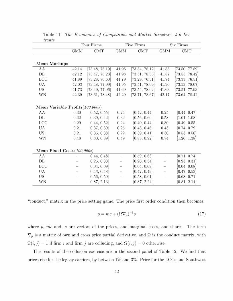
Table 11: The Economics of Competition and Market Structure, 4-6 En-trants

Four Firms Five Firms Six Firms

GMM CMT GMM CMT GMM CMT

Mean Markups

AA 42.14 [73.48, 78.19] 41.96 [73.54, 78.12] 41.85 [73.50, 77.89]DL 42.12 [73.47, 78.23] 41.98 [73.51, 78.33] 41.87 [73.55, 78.42]LCC 41.89 [73.28, 76.60] 41.79 [73.29, 76.51] 41.74 [73.33, 76.51]UA 42.03 [73.48, 77.99] 41.95 [73.51, 78.09] 41.90 [73.53, 78.07]US 41.73 [73.49, 77.96] 41.69 [73.54, 78.02] 41.63 [73.51, 77.93]WN 42.39 [73.61, 78.48] 42.29 [73.71, 78.67] 42.17 [73.64, 78.42]

Mean Variable Profits(100,000s)

AA 0.30 [0.52, 0.55] 0.24 [0.42, 0.44] 0.25 [0.44, 0.47]DL 0.22 [0.39, 0.42] 0.32 [0.56, 0.60] 0.58 [1.01, 1.08]LCC 0.29 [0.44, 0.52] 0.24 [0.40, 0.44] 0.30 [0.49, 0.55]UA 0.21 [0.37, 0.39] 0.25 [0.43, 0.46] 0.43 [0.74, 0.79]US 0.21 [0.36, 0.38] 0.22 [0.39, 0.41] 0.30 [0.53, 0.56]WN 0.48 [0.80, 0.89] 0.49 [0.83, 0.92] 0.74 [1.26, 1.38]

Mean Fixed Costs(100,000s)

AA – [0.44, 0.48] – [0.59, 0.63] – [0.71, 0.74]DL – [0.26, 0.33] – [0.26, 0.34] – [0.23, 0.31]LCC – [0.04, 0.09] – [0.04, 0.09] – [0.04, 0.08]UA – [0.43, 0.48] – [0.42, 0.49] – [0.47, 0.53]US – [0.56, 0.59] – [0.58, 0.61] – [0.68, 0.71]WN – [0.87, 2.13] – [0.87, 2.24] – [0.81, 2.14]

“conduct,” matrix in the price setting game. The price first order condition then becomes:

p = mc+ (Ω∇p)−1s (17)

where p, mc and, s are vectors of the prices, and marginal costs, and shares. The term

∇p is a matrix of own and cross price partial derivative, and Ω is the conduct matrix, with

Ω(i, j) = 1 if firm i and firm j are colluding, and Ω(i, j) = 0 otherwise.

The results of the collusion exercise are in the second panel of Table 12. We find that

prices rise for the legacy carriers, by between 1% and 3%. Price for the LCCs and Southwest

42

do not change. Also, there is virtually no change in the entry probabilities.

Next, we simulate a merger between American and US Air. Specifically, to do this we

change two features of the model. First, we allow the two airlines to internalize pricing

decisions on each others’ profit maximization problem. Second, for each market, we assign

the minimum costs of the two firms to both firms. For example, if both firms are potential

entrants in the PHL-CLT route, and US Air has cheaper marginal costs and fixed costs for

operating this route, then we assign US Air’s cost to American for this route.23

The results of the merger are presented in the third panel of Table 12. Both merged firm’s

prices rise, although the prices of the other firms largely stay the same, with the exception

of Southwest, who is forced to slightly decrease prices on average. Entry largely stays the

same, except now American enters between 3% and 8% more markets. This increased entry

could be due to the efficiency gains from the merger, or do to American having increased

market power because they do not need to compete against US Air, and therefore greater

pricing power in market where they are potential entrants. This second point will depend

crucially on the number of routes the two firms shared as potential entrants pre-merger.

23Note: although we are simulating a merger, we are allowing both firms to continue to exist in the market.In a sense, it is like an acquisition of one firm by the other firm’s parent company, with continued operationof both firms as separate entities.

43

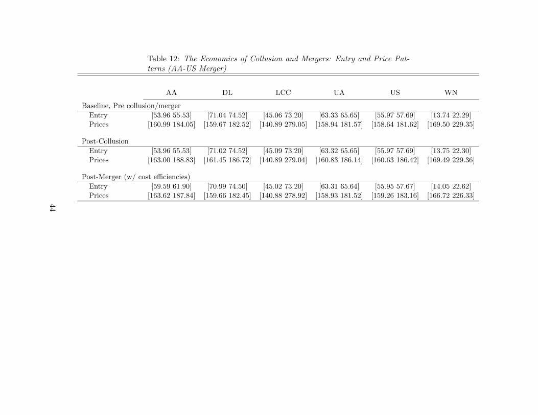
Table 12: The Economics of Collusion and Mergers: Entry and Price Pat-terns (AA-US Merger)

AA DL LCC UA US WN

Baseline, Pre collusion/merger

Entry [53.96 55.53] [71.04 74.52] [45.06 73.20] [63.33 65.65] [55.97 57.69] [13.74 22.29]Prices [160.99 184.05] [159.67 182.52] [140.89 279.05] [158.94 181.57] [158.64 181.62] [169.50 229.35]

Post-Collusion

Entry [53.96 55.53] [71.02 74.52] [45.09 73.20] [63.32 65.65] [55.97 57.69] [13.75 22.30]Prices [163.00 188.83] [161.45 186.72] [140.89 279.04] [160.83 186.14] [160.63 186.42] [169.49 229.36]

Post-Merger (w/ cost efficiencies)

Entry [59.59 61.90] [70.99 74.50] [45.02 73.20] [63.31 65.64] [55.95 57.67] [14.05 22.62]Prices [163.62 187.84] [159.66 182.45] [140.88 278.92] [158.93 181.52] [159.26 183.16] [166.72 226.33]

44

7 Conclusions

We propose a way to account for self-selection of firms into markets when we measure market

power and run counterfactual exercises in static models of competition. The study of the

effects of changes in market structure or in the legal setting of an industry on market power

and the welfare of consumers and firms is of primary interest for industrial organization

economists, both academics and researchers involved in antitrust and policy activities. In

addition, there is scope for an extension of this research in the closely related field of market-

ing, where one could use this methodology to study how the introduction of new products

changes the nature of competition in a market.

The methodology can be applied to economic contexts that can be modeled as a simul-

taneous, static, complete information game where economic agents make both discrete and

continuous choices. For example, it can be applied to estimate a model of household behavior

where a husband and a wife must decide whether to work and how many hours.

Thus, this research should be of interest to a wide range of industrial organization

economists, both academics and researchers involved in the design and implementation of

antitrust laws. Most importantly, the methodology proposed can be applied in all economic

contexts where agents interact strategically and make both discrete and continuous decisions.

45

References

Berry, Steven and Panle Jia. 2010. “Tracing the Woes: An Empirical Analysis of the Airline

Industry.” American Economic Journal: Microeconomics 2 (3):1–43.

Berry, Steven, James Levinsohn, and Ariel Pakes. 1995. “Automobile prices in market

equilibrium.” Econometrica: Journal of the Econometric Society :841–890.

Berry, Steven T. 1990. “Airport presence as product differentiation.” The American Eco-

nomic Review :394–399.

———. 1992. “Estimation of a Model of Entry in the Airline Industry.” Econometrica:

Journal of the Econometric Society :889–917.

———. 1994. “Estimating discrete-choice models of product differentiation.” The RAND

Journal of Economics :242–262.

———. 1999. “Free entry and social inefficiency in radio broadcasting.” The RAND Journal

of Economics 30 (3):397–420.

Bresnahan, Timothy F. 1987. “Competition and collusion in the American automobile in-

dustry: The 1955 price war.” The Journal of Industrial Economics :457–482.

———. 1989. “Empirical studies of industries with market power.” Handbook of industrial

organization 2:1011–1057.

Bresnahan, Timothy F and Peter C Reiss. 1990. “Entry in monopoly market.” The Review

of Economic Studies 57 (4):531–553.

———. 1991. “Entry and competition in concentrated markets.” Journal of Political Econ-

omy :977–1009.

Brueckner, Jan K and Pablo T Spiller. 1994. “Economies of traffic density in the deregulated

airline industry.” Journal of Law and Economics :379–415.

46

Chernozhukov, Victor, Han Hong, and Elie Tamer. 2007. “Estimation and confidence regions

for parameter sets in econometric models1.” Econometrica 75 (5):1243–1284.

Ciliberto, Federico, Amalia Miller, Helena Skyt Nielsen, and Marianne Simonsen. 2010.

“Playing the fertility game at work.” Unpublished manuscript .

Ciliberto, Federico and Elie Tamer. 2009. “Market structure and multiple equilibria in airline

markets.” Econometrica 77 (6):1791–1828.

Ciliberto, Federico and Jonathan W Williams. 2014. “Does Multimarket Contact Facilitate

Tacit Collusion? Inference on Conduct Parameters in the Airline Industry.” Inference on

Conduct Parameters in the Airline Industry (February 12, 2014) .

Cohen, Andrew M and Michael J Mazzeo. 2007. “Market structure and competition among

retail depository institutions.” The Review of Economics and Statistics 89 (1):60–74.

Draganska, Michaela, Michael Mazzeo, and Katja Seim. 2009. “Beyond plain vanilla: Mod-

eling joint product assortment and pricing decisions.” QME 7 (2):105–146.

Eizenberg, Alon. 2014. “Upstream Innovation and Product Variety in the US Home PC

Market*.” The Review of Economic Studies :rdu004.

Elzinga, Kenneth G and David E Mills. 2009. “Predatory Pricing in the Airline Industry:

Spirit Airlines v. Northwest Airlines (2005).” The Antitrust Revolution, 5th Edition, edited

by J. Kwoka and L. White, Forthcoming .

Goeree, Michelle Sovinsky. 2008. “Limited information and advertising in the US personal

computer industry.” Econometrica 76 (5):1017–1074.

Goolsbee, Austan and Chad Syverson. 2008. “How Do Incumbents Respond to the Threat

of Entry? Evidence from the Major Airlines.” The Quarterly Journal of Economics

123 (4):1611–1633.

47

Gronau, Reuben. 1974. “Wage Comparisons–A Selectivity Bias.” The Journal of Political

Economy :1119–1143.

Heckman, James J. 1976. “The common structure of statistical models of truncation, sample

selection and limited dependent variables and a simple estimator for such models.” In

Annals of Economic and Social Measurement, Volume 5, number 4. NBER, 475–492.

———. 1979. “Sample selection bias as a specification error.” Econometrica: Journal of the

econometric society :153–161.

Ho, Katherine. 2008. “Insurer-Provider Networks in the Medical Care Market.” American

Economic .

Mazzeo, Michael J. 2002. “Product choice and oligopoly market structure.” RAND Journal

of Economics :221–242.

Nevo, Aviv. 2001. “Measuring market power in the ready-to-eat cereal industry.” Econo-

metrica 69 (2):307–342.

Pakes, Ariel, J Porter, Joy Ishii, and Kate Ho. 2015. “Moment Inequalities and Their

Application.” Econometrica 83:315–334.

Panzar, John C. 1979. “Equilibrium and welfare in unregulated airline markets.” The

American Economic Review :92–95.

Reiss, Peter C and Pablo T Spiller. 1989. “Competition and entry in small airline markets.”

Journal of Law and Economics :S179–S202.

Roberts, Jimmy and Andrew Sweeting. 2014. “The Potential Entry Defense in Airline Merg-

ers.” working paper, Duke University .

Rosse, James N. 1970. “Estimating cost function parameters without using cost data: Illus-

trated methodology.” Econometrica: Journal of the Econometric Society :256–275.

48

Schmalensee, Richard. 1989. “Inter-industry studies of structure and performance.” Hand-

book of industrial organization 2 2.

Seim, Katja. 2006. “An empirical model of firm entry with endogenous product-type choices.”

RAND Journal of Economics :619–640.

Tamer, Elie. 2003. “Incomplete simultaneous discrete response model with multiple equilib-

ria.” The Review of Economic Studies 70 (1):147–165.

49

A Computational Issues

A.1 Computational Resources

This section has been developed with Ed Hall at the University of Virginia. Ed Hall works

as a staff member of the University of Virginia Advanced Computing and Engagement

(UVACSE) group. Ed Hall has worked with Federico Ciliberto, Charles Murry, and Elie

Tamer on the Matlab code development and optimization as part of an ongoing UVACSE

“Tiger Team” project.

The simulation code is written in Matlab, and applies the simulated annealing and pattern

search algorithms from the global optimization toolbox in sequence to minimize the distance

function given by Equation (5). The strategy is to use simulated annealing to converge to the

region where the global minimum is located, and then the pattern search will converge more

quickly toward the global minimum. In addition, using simulated annealing and pattern

search algorithms provide a sampling of the distance function that is more complete as

they follow a path toward the minimum than using other nongradient-based algorithms such

Nelder-Mead. Essentially, we use the optimization algorithm to sample the objective function

and we save the results to get a snapshot of the surface of the function.

The minimization of the distance function is computationally expensive because we have

to use simulation methods to integrate two distribution functions and then compare them.

In addition, we need to solve for Nash equilibria in many markets, and for many possible

combinations of firms in each market. We speed up the evaluation of the objective function by

parallelizing the computation of the integrals across markets that share common observable

characteristics, using the Matlab parfor construct.

For each problem specification, we started our search from the true parameter value in

the Monte Carlo exercise and at least 5 initial values in the empirical exercise. From the

overall minimum, we ran simulated annealing for a while longer to evaluate the functions

at many different parameter values close to the minimum we found. We ran the code on

the XSEDE resources Gordon and Trestles at the San Diego Supercomputing Center. Given

50

the 48 hour job runtime limit, we allowed the simulated annealing algorithm to work on

convergence for one day by limiting the number of algorithm iteration to 2000, then passed

the current best parameter vector to the pattern search algorithm and allowed an additional

day for that algorithm to minimize the distance function. The code periodically saved the

state information necessary to restart from where it left off when it exceeds the 48 hour time

limit.

Performance and scaling tests on Gordon indicated 32 workers (cores) provide the shortest

execution time before communication overhead to the workers becomes significant. We also

found that there is a dramatic improvement in the precision of our estimates when we run

400 simulations instead of a 100.24

The computationally intense estimation of our models in a relatively short period of time

was made feasible because of the use of XSEDE resources.25

We also used the HPC System at U.Va. known as Rivanna. Rivanna is a 4800-core,

high-speed interconnect cluster, with 1.4 PBs of storage available in a fast Lustre filesystem.

Simulations on this platform were primarily used to test the code before running it on the

XSEDE resources. We gratefully acknowledge the use of both the XSEDE resources and

those at the University of Virginia.

A.2 Practical Computational Solutions

As Figure 1 illustrates, minimizing the distance function given by Equation 5 consists of min-

imizing an appropriately defined distance between the ”true” CDF of the unobservables and

the CDF of the model-predicted unobservables. In practice, we found that it worked better

to minimize the distance between set coverage - a kind of a histogram - of the unobservables

and its corresponding model-predicted histogram.

24We have also experimented using 1,000 simulations but the results were not more precise than when weused 400.

25John Towns, Timothy Cockerill, Maytal Dahan, Ian Foster, Kelly Gaither, Andrew Grimshaw, VictorHazlewood, Scott Lathrop, Dave Lifka, Gregory D. Peterson, Ralph Roskies, J. Ray Scott, Nancy Wilkens-Diehr, “XSEDE: Accelerating Scientific Discovery”, Computing in Science & Engineering, vol.16, no. 5, pp.62-74, Sept.-Oct. 2014.

51

To minimize the distance of the bin functions one would want to use a large number of

bins over the support of the unobservables. However, we have found that using as few bins as

six equally sized intervals provides excellent results, where the smallest and largest numbers

are derived from the distribution of the residuals that we obtain when we run the GMM

estimates. We take the minimum and maximum of those values and multiply them by 2.5.

B Data Construction

The construction of the data is largely similar to the approach taken in Ciliberto and Tamer

(2009). We refer the reader to the Supplemental Material (Ciliberto and Tamer [2009b]).

The main data are from the domestic Origin and Destination Survey (DB1B), the Form

41 Traffic T-100 Domestic Segment (U.S. Carriers), and the Aviation Support Tables : Car-

rier Decode, all available from the Department of Transportation’s National Transportation

Library/ We also use the US Census for the demographic data, specifically to get the to-

tal population in each Metropolitan Statistical Area. The Origin and Destination Survey

(DB1B) is a 10 percent sample of airline tickets from reporting carriers. The dataset includes

information on the origin, destination, and other itinerary details of passengers transported,

most importantly the fare. The Form 41 Traffic T-100 Domestic Segment (U.S. Carriers)

contains domestic non-stop segment data reported by US carriers, including carrier, ori-

gin, destination of the trip. The dataset Aviation Support Tables : Carrier Decode is used

to clean the information on carriers, more specifically to determine which carriers exit the

industry over time, and which one merge, or are owned by another carrier.

We define a market as a unidirectional trip between two airports, irrespective of inter-

mediate transfer points. For example, we will assume that the nonstop service between

Chicago O’Hare (ORD) and New York La Guardia (LGA) is in the same market as the

connecting service through Cleveland (CLE) from ORD to LGA. We assume that flights

to different airports in the same metropolitan area are in separate markets. To select the

markets, we merge this dataset with demographic information on population from the U.S.

Census Bureau for all the Metropolitan Statistical Areas of the United States. We then

52

construct a ranking of airports by the MSA’s market size. The dataset includes a sample

of markets between the top 100 Metropolitan Statistical Areas, ranked by the population

size. We exclude the Youngstown-Warren Regional Airport, Toledo Express Airport, St.

Pete-Clearwater International Airport, Muskegon County Airport, and Lansing Capital Re-

gion International Airport because there are too few markets between these airports and the

remaining airports.

Then, we proceed to further clean the data as follows. We drop: 1) Tickets with more than

6 coupons; 2) Tickets involving US-nonreporting carrier flying within North America (small

airlines serving big airlines) and foreign carrier flying between two US points; 3) Tickets that

are part of international travel; 4) Tickets involving non-contiguous domestic travel (Hawaii,

Alaska, and Territories) as these flights are subsidized by the US mail service; 5) Tickets

whose fare credibility is questioned by the DOT; 6) Tickets that are neither one-way nor

round-trip travel; 7) Tickets including travel on more than one airline on a directional trip

(known as interline tickets); 8) Tickets with fares less than 20 dollars; 9) Tickets in the top

and bottom five percentiles of the year-quarter fare distribution.

We then aggregate the ticket data by ticketing carrier and thus the unit of observation

now is market-carrier-year-quarter specific.

Next, we determine the markets that are not served by any airline, but that could be

potentially served by one. These are the markets that were served at least 90 percent of the

quarters. We drop markets whose distance is less than 150 miles. We also drop airlines that

served fewer than 20 passengers in a quarter.

The airlines in the initial dataset are: American, Alaska, JetBlue, Delta, Frontier, Air-

Tran, Allegiant, Spirit, Sun Country, United, USAir, Virgin, Southwest. As in Ciliberto and

Tamer (2009), we deal with how to treat regional airlines that operate through code-sharing

with national airlines as follows. We assume that the decision to serve a spoke is made by

the regional carrier, which then signs code-share agreements with the national airlines. As

long as the regional airline is independently owned and issues tickets, we treat it separately

from the national airline.

53

The low cost type is composed of: Alaska, JetBlue, Frontier, AirTran, Allegiant, Spirit,

Sun Country, Virgin. We re-elaborate their data as follows. The LCC’s number of passengers

is the sum of the passengers over all the LCCs that serve a market. The LCC’s price is the

passenger weighted mean of the prices charged by all the LCC airlines in a market. For

the explanatory variables we take the maximum value among the low cost carriers serving

a market of the variables Origin Presence, Destination Presence, Nonstop Network Origin,

Nonstop Network Destination. We also take the maximum of the categorical variables that

indicate whether a firm is a potential entrant in a market.

After this preliminary cleaning, we are left with 34,643 market-carrier observations and

10,421 markets. Next, we compute the 5 and 95 percentile of the prices, shares and market

size, and we drop markets where those prices, shares, and market sizes were observed. This

leads us to the final sample: 20,642 market-carrier observations and 6,322 markets.

To compute the confidence intervals as in Chernozhukov, Hong, and Tamer (2007) we

discretize the exogenous variables. The discretization is done as follows. First, we standardize

the variables. Then, we construct intervals where the thresholds are given by -1, 0, 1, as well

as integers such as -2, 2, -3, 3. Most of the observations are in the intervals [-1,0] and [0,1].

C Monte Carlo Experiments

We run Monte Carlo experiments to test the methodology on our full equilibrium model,

presented in Section 3.1. More specifically, using different random seeds we generate data

under a particular parametric specification of the model. We then estimate the model using

a standard GMM framework as well as our proposed methodology. We provide specifics and

report results below.

We consider the case of 10,000 simulated markets, where, in each market m, there are

Km potential firms and each firm must decide, simultaneously, whether to serve a market

and the prices they charge conditional on serving the market. We allow for the identity and

number of potential entrants vary by market, from a minimum of one to a maximum of four,

and generate this randomly.

54

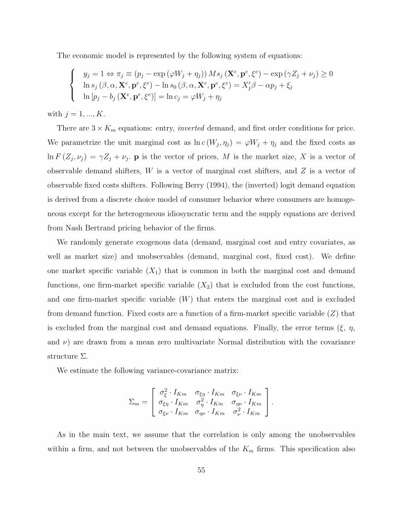
The economic model is represented by the following system of equations:yj = 1⇔ πj ≡ (pj − exp (ϕWj + ηj))Msj (Xe,pe, ξe)− exp (γZj + νj) ≥ 0

ln sj (β, α,Xe,pe, ξe)− ln s0 (β, α,Xe,pe, ξe) = X ′jβ − αpj + ξj

ln [pj − bj (Xe,pe, ξe)] = ln cj = ϕWj + ηj

with j = 1, ..., K.

There are 3×Km equations: entry, inverted demand, and first order conditions for price.

We parametrize the unit marginal cost as ln c (Wj, ηj) = ϕWj + ηj and the fixed costs as

lnF (Zj, νj) = γZj + νj. p is the vector of prices, M is the market size, X is a vector of

observable demand shifters, W is a vector of marginal cost shifters, and Z is a vector of

observable fixed costs shifters. Following Berry (1994), the (inverted) logit demand equation

is derived from a discrete choice model of consumer behavior where consumers are homoge-

neous except for the heterogeneous idiosyncratic term and the supply equations are derived

from Nash Bertrand pricing behavior of the firms.

We randomly generate exogenous data (demand, marginal cost and entry covariates, as

well as market size) and unobservables (demand, marginal cost, fixed cost). We define

one market specific variable (X1) that is common in both the marginal cost and demand

functions, one firm-market specific variable (X2) that is excluded from the cost functions,

and one firm-market specific variable (W ) that enters the marginal cost and is excluded

from demand function. Fixed costs are a function of a firm-market specific variable (Z) that

is excluded from the marginal cost and demand equations. Finally, the error terms (ξ, η,

and ν) are drawn from a mean zero multivariate Normal distribution with the covariance

structure Σ.

We estimate the following variance-covariance matrix:

Σm =

σ2ξ · IKm σξη · IKm σξν · IKm

σξη · IKm σ2η · IKm σην · IKm

σξν · IKm σην · IKm σ2ν · IKm

.As in the main text, we assume that the correlation is only among the unobservables

within a firm, and not between the unobservables of the Km firms. This specification also

55

restricts the correlations to be the same for each firm and clearly reduces the parameters to

be estimated. However, the specification is rich compared to existing methods.

For each covariate and for each firm (or market for the case of X1), we generate a random

number from an independent standard uniform distribution. We then create three bins

between zero and one for each covariate to generate the discrete variable. We also randomly

generate a market size for each market, between 100,000 and 1,000,000.

For each firm in each market and a given vector of true parameter values, θtrue, which

is reported in Column 1 of Table A1, we solve for the equilibrium prices, shares, and entry

decisions of the model described above. This is repeated for all simulations.

Note that the exogenous variables X1, X2,W, Z are generated independently of the

unobservables ξ, η, and ν, in the full sample (before entry). However, we will show that

at an equilibrium of the model the optimal entry and price decisions of the firms introduce

correlation between the unobservables and the exogenous data. This is so because firms that

are a better fit into the market in terms of observables and unobservables are more likely to

enter.

GMM Estimation. We estimate the parameters of the marginal cost and demand functions

using the conditional moment conditions E [ξj| (Xj,Wj, X−j)] = 0. We present the 90%

confidence interval across simulations in Column 2 of Table A1. Some of the results are close

to the true values. But, others, such as marginal cost estimates are clearly biased. It is

interesting to note also that the price parameter is consistently estimated to be larger than

the truth.

We find that a standard instrumental variable approach does not solve the selection prob-

lem. In particular, the usual moment condition E[ξ1|X1, X2,W, Z] = 0 does not generally

imply that E[ξ1|X1, X2,W, Z, y1 = 1] = 0, where ξ1 is the demand unobservable.26 Firms

that enter have a high value for ξ1, on average, which invalidates the mean zero condition.

We show that the standard approach (Bresnahan, 1987; Berry, 1994; Berry, Levinsohn, and

26We explain the method by looking at the demand unobservable, but an analogous argument can be madefor the marginal cost unobservables.

56

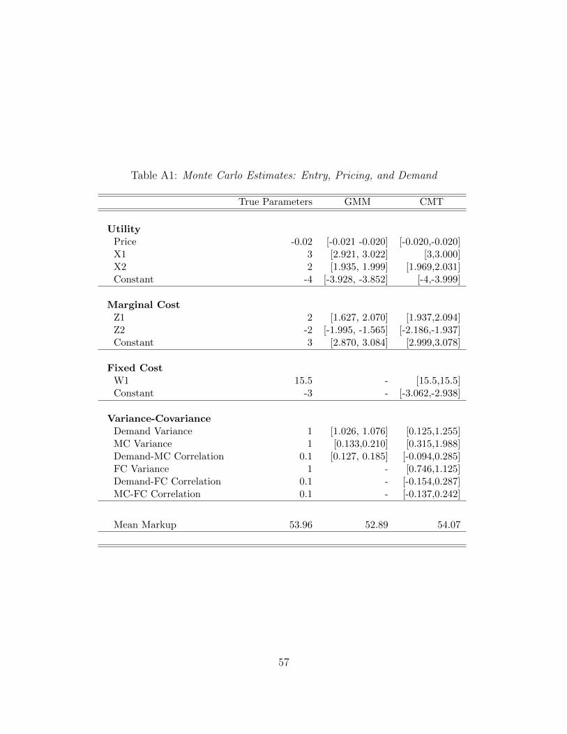
Table A1: Monte Carlo Estimates: Entry, Pricing, and Demand

True Parameters GMM CMT

UtilityPrice -0.02 [-0.021 -0.020] [-0.020,-0.020]X1 3 [2.921, 3.022] [3,3.000]X2 2 [1.935, 1.999] [1.969,2.031]Constant -4 [-3.928, -3.852] [-4,-3.999]

Marginal CostZ1 2 [1.627, 2.070] [1.937,2.094]Z2 -2 [-1.995, -1.565] [-2.186,-1.937]Constant 3 [2.870, 3.084] [2.999,3.078]

Fixed CostW1 15.5 - [15.5,15.5]Constant -3 - [-3.062,-2.938]

Variance-CovarianceDemand Variance 1 [1.026, 1.076] [0.125,1.255]MC Variance 1 [0.133,0.210] [0.315,1.988]Demand-MC Correlation 0.1 [0.127, 0.185] [-0.094,0.285]FC Variance 1 - [0.746,1.125]Demand-FC Correlation 0.1 - [-0.154,0.287]MC-FC Correlation 0.1 - [-0.137,0.242]

Mean Markup 53.96 52.89 54.07

57

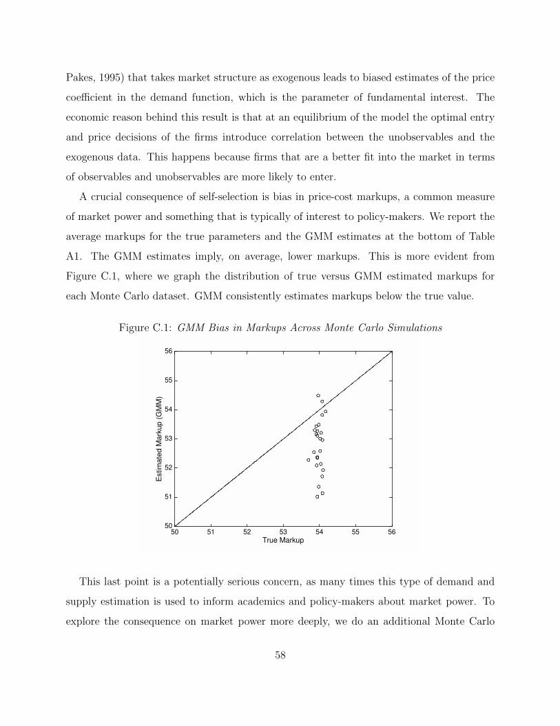
Pakes, 1995) that takes market structure as exogenous leads to biased estimates of the price

coefficient in the demand function, which is the parameter of fundamental interest. The

economic reason behind this result is that at an equilibrium of the model the optimal entry

and price decisions of the firms introduce correlation between the unobservables and the

exogenous data. This happens because firms that are a better fit into the market in terms

of observables and unobservables are more likely to enter.

A crucial consequence of self-selection is bias in price-cost markups, a common measure

of market power and something that is typically of interest to policy-makers. We report the

average markups for the true parameters and the GMM estimates at the bottom of Table

A1. The GMM estimates imply, on average, lower markups. This is more evident from

Figure C.1, where we graph the distribution of true versus GMM estimated markups for

each Monte Carlo dataset. GMM consistently estimates markups below the true value.

Figure C.1: GMM Bias in Markups Across Monte Carlo Simulations

True Markup50 51 52 53 54 55 56

Estim

ate

d M

ark

up (

GM

M)

50

51

52

53

54

55

56

This last point is a potentially serious concern, as many times this type of demand and

supply estimation is used to inform academics and policy-makers about market power. To

explore the consequence on market power more deeply, we do an additional Monte Carlo

58

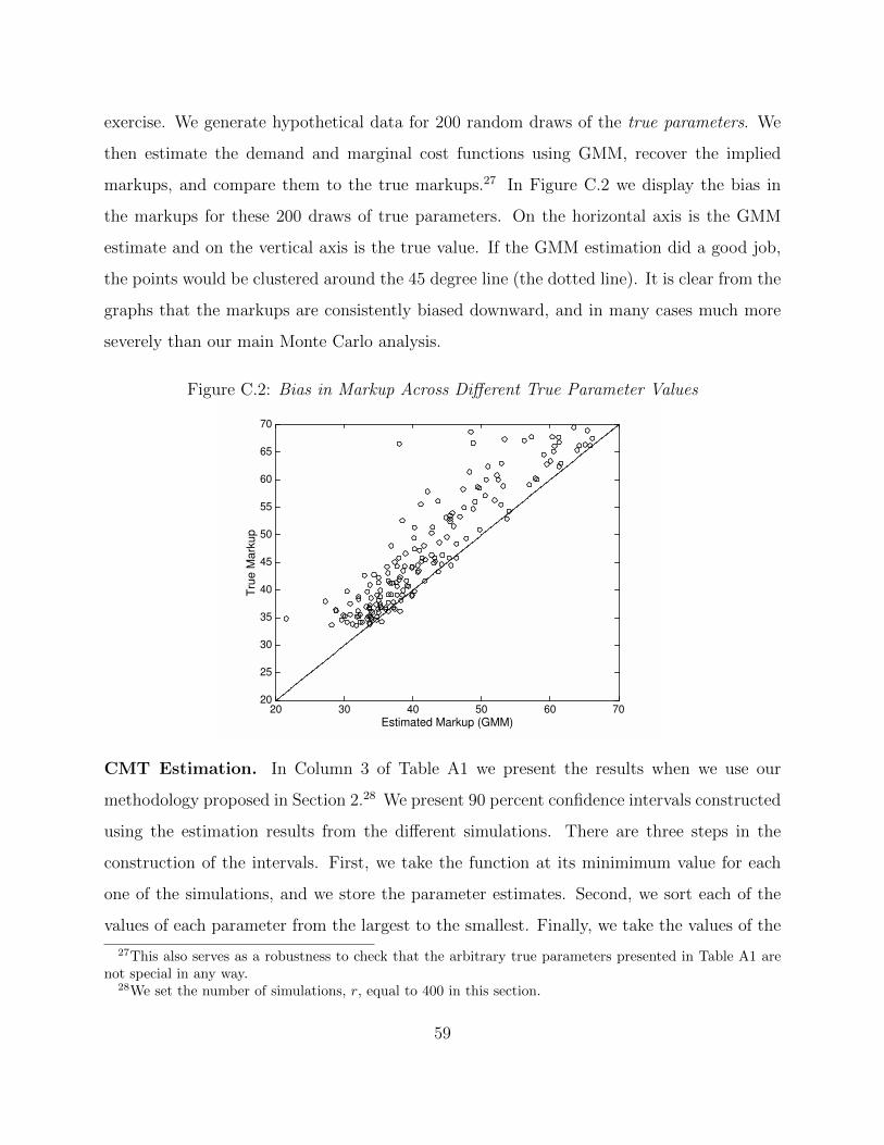
exercise. We generate hypothetical data for 200 random draws of the true parameters. We

then estimate the demand and marginal cost functions using GMM, recover the implied

markups, and compare them to the true markups.27 In Figure C.2 we display the bias in

the markups for these 200 draws of true parameters. On the horizontal axis is the GMM

estimate and on the vertical axis is the true value. If the GMM estimation did a good job,

the points would be clustered around the 45 degree line (the dotted line). It is clear from the

graphs that the markups are consistently biased downward, and in many cases much more

severely than our main Monte Carlo analysis.

Figure C.2: Bias in Markup Across Different True Parameter Values

Estimated Markup (GMM)20 30 40 50 60 70

Tru

e M

ark

up

20

25

30

35

40

45

50

55

60

65

70

CMT Estimation. In Column 3 of Table A1 we present the results when we use our

methodology proposed in Section 2.28 We present 90 percent confidence intervals constructed

using the estimation results from the different simulations. There are three steps in the

construction of the intervals. First, we take the function at its minimimum value for each

one of the simulations, and we store the parameter estimates. Second, we sort each of the

values of each parameter from the largest to the smallest. Finally, we take the values of the

27This also serves as a robustness to check that the arbitrary true parameters presented in Table A1 arenot special in any way.

28We set the number of simulations, r, equal to 400 in this section.

59

parameters at the 5th and 95th position.

We find that all of the true parameters fall within the confidence intervals. In other

words, different random seeds do not lead to different coefficient estimates, and because the

percentage of market-simulations when we observe multiple equilibria is 0.03. That is, out

of 5000*400=200,000 market-simulations, we only observe multiple equilibria in 30 of them.

In particular, the confidence interval of the price coefficient is [−0.02,−0.02], and it equals

the true value.

Because our model is a full equilibrium model with the entry conditions as well, we can

estimate the parameters of the fixed costs. Column 3 shows that the confidence intervals

cover both the true value of the constant and of the variable Z. The true variances are also

included in the estimated confidence intervals. For example, the variance of the unobservable

that enters into the fixed costs was set equal to 1 and the estimated confidence interval in

Column 3 is [0.746, 1.125].

We now turn to examining the fit of the results from our methodology by comparing key

results to the true data. We compare the observed and predicted entry patterns, as well as

features of profits, such as prices, markups, and total profits.

Consider first entry patterns for a specific Monte Carlo seed (the same one that we used

in the discussion of the distribution of potential entrants.)29. We present results from entry

patterns in Table A2. The cell in Row Firm1 and Column Real Data Share reports that

we observe Firm 1 serving 30.12 percentage of markets. The cell immediately to the right

reports that our model predicts that Firm 1 enters 24.68 percent of the time. The next cell

to the right in Row Firm1 and Column Match Percentage reports that in 88.17 percent of

the market-simulations we correctly predict entry, that is, either we correctly predict firm 1

to be in the market or we correctly predict firm 1 not to be in the market. In the remaining

11.83 percent of the market-simulations we do not have the right prediction. Lastly, we

evaluate how well we predict specific potential equilibria. For example, the fact that we have

four firms implies that we have 16 possible equilibrium configurations.

29Notice that we report a single number for sake of simplicity because the percentage of multiple equilibriais negligible

60

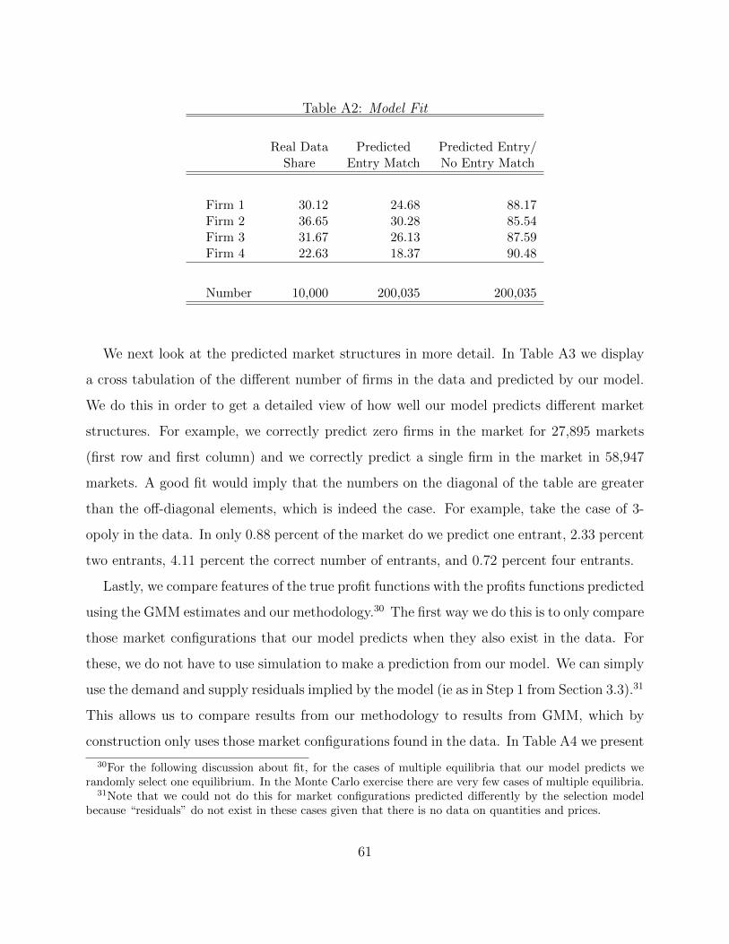
Table A2: Model Fit

Real Data Predicted Predicted Entry/Share Entry Match No Entry Match

Firm 1 30.12 24.68 88.17Firm 2 36.65 30.28 85.54Firm 3 31.67 26.13 87.59Firm 4 22.63 18.37 90.48

Number 10,000 200,035 200,035

We next look at the predicted market structures in more detail. In Table A3 we display

a cross tabulation of the different number of firms in the data and predicted by our model.

We do this in order to get a detailed view of how well our model predicts different market

structures. For example, we correctly predict zero firms in the market for 27,895 markets

(first row and first column) and we correctly predict a single firm in the market in 58,947

markets. A good fit would imply that the numbers on the diagonal of the table are greater

than the off-diagonal elements, which is indeed the case. For example, take the case of 3-

opoly in the data. In only 0.88 percent of the market do we predict one entrant, 2.33 percent

two entrants, 4.11 percent the correct number of entrants, and 0.72 percent four entrants.

Lastly, we compare features of the true profit functions with the profits functions predicted

using the GMM estimates and our methodology.30 The first way we do this is to only compare

those market configurations that our model predicts when they also exist in the data. For

these, we do not have to use simulation to make a prediction from our model. We can simply

use the demand and supply residuals implied by the model (ie as in Step 1 from Section 3.3).31

This allows us to compare results from our methodology to results from GMM, which by

construction only uses those market configurations found in the data. In Table A4 we present

30For the following discussion about fit, for the cases of multiple equilibria that our model predicts werandomly select one equilibrium. In the Monte Carlo exercise there are very few cases of multiple equilibria.

31Note that we could not do this for market configurations predicted differently by the selection modelbecause “residuals” do not exist in these cases given that there is no data on quantities and prices.

61

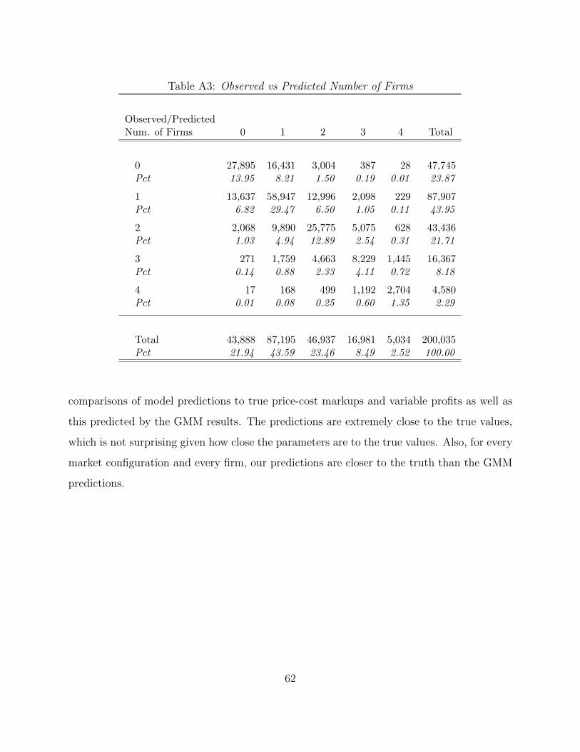
Table A3: Observed vs Predicted Number of Firms

Observed/PredictedNum. of Firms 0 1 2 3 4 Total

0 27,895 16,431 3,004 387 28 47,745Pct 13.95 8.21 1.50 0.19 0.01 23.87

1 13,637 58,947 12,996 2,098 229 87,907Pct 6.82 29.47 6.50 1.05 0.11 43.95

2 2,068 9,890 25,775 5,075 628 43,436Pct 1.03 4.94 12.89 2.54 0.31 21.71

3 271 1,759 4,663 8,229 1,445 16,367Pct 0.14 0.88 2.33 4.11 0.72 8.18

4 17 168 499 1,192 2,704 4,580Pct 0.01 0.08 0.25 0.60 1.35 2.29

Total 43,888 87,195 46,937 16,981 5,034 200,035Pct 21.94 43.59 23.46 8.49 2.52 100.00

comparisons of model predictions to true price-cost markups and variable profits as well as

this predicted by the GMM results. The predictions are extremely close to the true values,

which is not surprising given how close the parameters are to the true values. Also, for every

market configuration and every firm, our predictions are closer to the truth than the GMM

predictions.

62

Table A4: The Economics of Market Structure Using the Estimation Resid-uals

Monopoly Duopoly Three Firms Four Firms

True GMM Pred. True GMM Pred. True GMM Pred. True GMM Pred.

Mean Markups

1 54.40 53.83 54.38 53.71 53.15 53.71 53.86 53.30 53.87 53.68 53.11 53.672 53.95 53.38 53.93 53.69 53.12 53.68 53.61 53.04 53.61 53.71 53.14 53.723 54.24 53.67 54.23 54.00 53.43 53.99 53.52 52.96 53.52 53.68 53.11 53.704 54.07 53.50 54.07 54.02 53.45 54.00 53.40 52.84 53.40 53.69 53.12 53.70

Mean Variable Profits(100,000s)

1 48.07 47.35 47.85 44.27 43.75 44.25 49.02 48.39 48.93 48.03 47.35 47.872 42.09 41.40 41.85 43.67 43.13 43.61 46.61 46.12 46.64 49.72 49.29 49.863 46.58 45.86 46.36 45.46 44.79 45.28 45.54 44.96 45.46 49.28 48.97 49.564 44.03 43.44 43.93 47.61 46.87 47.38 44.91 44.30 44.79 50.09 49.61 50.18

63

The second way we compare features of the profit functions is to simulate profits using our

estimated parameters and our model of selection, without the restriction that the predicted

market configurations must match those in the data. This is exactly the benefit of using

our model; we can make predictions out of sample equilibrium market configurations. We

present comparisons of price, markups, and profits in Table A5. In the first panel we present

price, in the second panel we present markups, in the third panel we present variable profits

(in 100,000s), and in the fourth panel we present total profits (in 100,000s). In all cases we

present the true and predicted mean values by the number of firms in the market. Overall,

our predictions match the data very well. There is non-monotonicity in markups across

the number of market participants. This is a direct consequence of selection into markets

based on observable and unobservable firm and market attributes. Markets that support

three entrants may be better along some dimension than markets that supports one entrant.

For example a high demand shock or low cost shock may cause more entry in a particular

market. Those reasons for entry also effect equilibrium prices. For example, if a market has

a high demand shock, then more firms might enter and prices might be higher than a low

demand shock market with a single entrant.

64

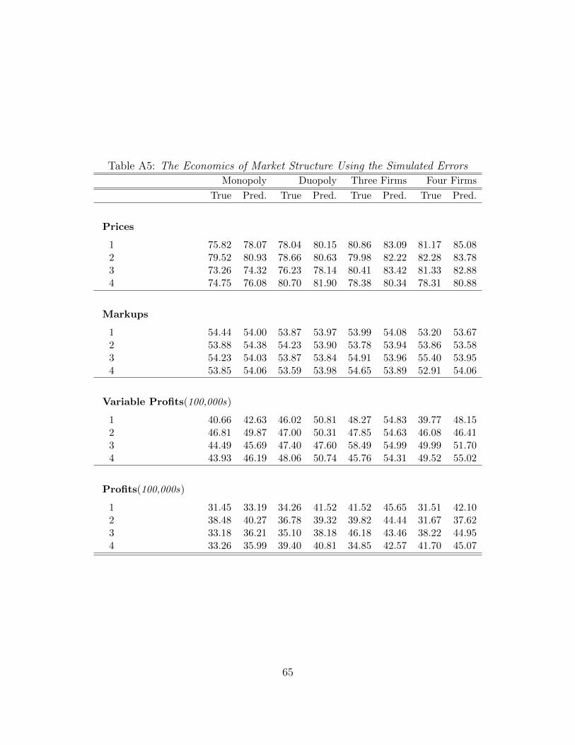
Table A5: The Economics of Market Structure Using the Simulated Errors

Monopoly Duopoly Three Firms Four Firms

True Pred. True Pred. True Pred. True Pred.

Prices

1 75.82 78.07 78.04 80.15 80.86 83.09 81.17 85.082 79.52 80.93 78.66 80.63 79.98 82.22 82.28 83.783 73.26 74.32 76.23 78.14 80.41 83.42 81.33 82.884 74.75 76.08 80.70 81.90 78.38 80.34 78.31 80.88

Markups

1 54.44 54.00 53.87 53.97 53.99 54.08 53.20 53.672 53.88 54.38 54.23 53.90 53.78 53.94 53.86 53.583 54.23 54.03 53.87 53.84 54.91 53.96 55.40 53.954 53.85 54.06 53.59 53.98 54.65 53.89 52.91 54.06

Variable Profits(100,000s)

1 40.66 42.63 46.02 50.81 48.27 54.83 39.77 48.152 46.81 49.87 47.00 50.31 47.85 54.63 46.08 46.413 44.49 45.69 47.40 47.60 58.49 54.99 49.99 51.704 43.93 46.19 48.06 50.74 45.76 54.31 49.52 55.02

Profits(100,000s)

1 31.45 33.19 34.26 41.52 41.52 45.65 31.51 42.102 38.48 40.27 36.78 39.32 39.82 44.44 31.67 37.623 33.18 36.21 35.10 38.18 46.18 43.46 38.22 44.954 33.26 35.99 39.40 40.81 34.85 42.57 41.70 45.07

65