Market Price Manipulation in a Sequential Trade Model∗

Shino Takayama†

University of Queensland

Abstract. The dynamic version of the Glosten and Milgrom (1985) model of asset pricing with asym-metric information is studied. It is shown that there is a unique equilibrium when the next-period valuefunction of the informed trader, who knows the terminal value of the asset, is strictly convex and strictlymonotone in terms of the market maker’s prior belief. A characterization of the bid and ask prices andthe informed trader’s manipulative strategy in equilibrium is given. Finally, a computational methodfor simulating the equilibrium is presented.

Key Words: Market microstructure; Glosten-Milgrom; Price formation; Sequential trade; Asymmetricinformation; Trade size; Bid-ask spreads.JEL Classification Numbers: D82, G12.

∗I am grateful to Andrew McLennan, Jan Werner, Myrna Wooders, Rabee Tourky and Han Ozsoylev. Also, I would like tothank Simon Grant, John Hillas, Dmitriy Kvasov and other participants at the International Conference on Economic Theoryin Kyoto, the 26th Australasian Economic Theory Workshop, Public Economic Theory Conference in Seoul, EconometricSociety Australasian Meeting in 2008 and seminar participants at the University of Queensland, Australian National Univer-sity, University of Auckland, and Osaka University for helpful comments on an earlier version of this paper. I also thankAubrey Clark for his excellent proofreading. All errors remaining are my own.†Takayama (corresponding author); School of Economics, University of Queensland, Level 6 - Colin Clark Building (39),

St Lucia, QLD 4072, Australia; e-mail: shino.mclennan@gmail.com; tel: +61-7-3346-7379; fax: +61-7-3365-7299.

1 Introduction

This paper develops a model of dynamic informed trading from a canonical framework in the marketmicrostructure literature and characterizes an equilibrium. In asymmetric information models of finan-cial markets, trading behavior imperfectly reveals the private information held by traders. Informedtraders who trade dynamically thus have an incentive not only to trade less aggressively but also tomanipulate the market by trading in the wrong direction, undertaking short-term losses to confuse themarket and then recouping the losses in the future. Dynamic trading and price manipulation by aninformed trader have been a challenging issue in the literature of market microstructure.

There are two standard reference frameworks in the literature. The first is called the “continuousauction framework” first developed by Kyle (1985). The second is the “sequential trade framework”proposed by Glosten and Milgrom (1985). A large amount of research has been done involving theapplication of these two frameworks. Both frameworks are sufficiently simple and well behaved thatthey easily lend themselves to analysis of policy issues and empirical testing (see Madhavan (2000) andBiais et al. (2005) for extensive surveys of the literature).

One of the simplifying assumptions in Glosten and Milgrom (1985) is that traders can trade onlyonce. In the original Glosten-Milgrom model manipulation does not occur because there is no chanceto re-trade and as a result traders maximize their one-period payoff. In the Kyle model the informedtrader’s strategy is monotonic in the sense that she buys the asset when it is undervalued given herinformation and vice versa; dynamic price manipulation is ruled out by assumption.

This paper follows the strand of the sequential trade framework developed by Glosten and Mil-grom. This paper considers markets where a risky asset is traded for finitely many periods betweencompetitive market makers, two types of strategic informed traders and liquidity traders. In the begin-ning of the game, nature chooses the liquidation value of a risky asset to be high or low and tells theinformed trader who trades dynamically. In each period there is a random determination of whetherthe informed trader or a liquidity trader trades. The market maker posts bid and ask prices for the nextperiod, after which the trader buys or sells one unit. The termination value is revealed at the end of thegame and the payoff for the informed trader is the sum of the termination value times net-holding of theasset and revenue from buying and selling the asset. Within the model described above we consider anequilibrium such that (a) the informed trader’s strategy is optimal beginning at any history; (b) marketmakers make zero profit in each period under their common Bayesian belief conditional on the historyand chosen trade; (c) liquidity traders trade for their exogenous liquidity needs.

There exist a large number of papers that theoretically and empirically examine price manipulationin different settings. For example, Jordan and Jordan (1996) examine Solomon Brothers’ market cornerof a Treasury note auction in May 1991. Felixson and Pelli (1999) examine closing price manipulationin the Finnish stock market. Mahoney (1999) examines stock price manipulation leading up to theSecurities Exchange Act of 1934. Vitale (2000) examines manipulation in the foreign exchange market.Merrick et al. (2005) examine a case of manipulation involving a delivery squeeze on a bond futures

2

contract traded in London. A recent paper by Aggarwal and Wu (2006) suggests that stock marketmanipulation may have important impacts on market efficiency. According to the empirical findings inAggarwal and Wu (2006), while manipulative activities seem to have declined on the main exchanges,it is still a serious issue in both developed and emerging financial markets, especially in the over-the-counter markets.

The theoretical literature starts with manipulation by uninformed traders. Allen and Gale (1992)provide a model of strategic trading in which some equilibria involve manipulation. Furthermore, Allenand Gorton (1992) consider a model of pure trade-based uninformed manipulation in which an asym-metry in buys and sells by liquidity traders creates the possibility of manipulation. The first paper toconsider manipulation by an informed trader within the discrete-time Glosten-Milgrom framework isChakraborty and Yilmaz (2004). They show that when the market faces uncertainty about the existenceof informed traders and there are a large number of trading periods long-lived informed traders willmanipulate in every equilibrium. On the other hand, Back and Baruch (2004) study the equivalenceof the Glosten-Milgrom model and the Kyle model in a continuous-time setting, and show that theequilibrium in the Glosten-Milgrom model is approximately the same as that in the Kyle model whenthe trade size is small and uninformed trades arrive frequently. They conclude that the continuous-timeKyle model is more tractable than the Glosten-Milgrom model, although most markets are organizedas in the sequential trade models. More recently there has been an interest in the informed trader’sdynamic strategy. Among others, Brunnermeier and Pedersen (2005) consider dynamic strategic be-havior of large traders and show that “overshooting” occurs in equilibrium. Back and Baruch (2007)analyze different market systems by allowing the informed traders to trade continuously within theGlosten-Milgrom framework.

Despite the importance of dynamic trading strategies by informed traders in the literature, charac-teristics of price dynamics and information transmission have not yet been adequately studied becausethere is no closed-form solution for equilibrium in the dynamic Glosten-Milgrom framework and it isnot yet known if equilibrium is unique either in the Kyle model (see Boulatov et al. (2005) for a furtherdevelopment) or the dynamic Glosten-Milgrom model in which strategic informed traders can traderepeatedly. In this paper we present a model of dynamic informed trading and show that there exists aunique equilibrium when the value functions of the informed traders are monotonic and strictly convexin terms of the market maker’s prior belief. In addition, we characterize the equilibrium bid and askprices and specify the necessary condition for manipulation to occur in equilibrium. Finally, we presenta computational method to solve for the equilibrium and comparative statics from the simulations.

It is worth mentioning that in Back and Baruch (2004) the equilibrium strategy of the informedtrader is not accurately simulated. This is because their model is a continuous-time stationary case andtheir program tries to find the value functions as a fixed point. To do this they use an extrapolationmethod which requires calculating the slopes of the value functions. In the region of beliefs at whichmanipulation arises the slopes of the value functions are very small. In fact, Back and Baruch (2004)

3

wrote that even though all the equilibrium conditions hold with a high order of accuracy, it appearsfrom their plots that the strategies are not estimated very accurately when manipulation arises and thisis probably an inevitable result of their estimation method, because the derivative of the value functionis small where manipulation arises (see Back and Baruch (2004) p.464, last paragraph).

This difficulty prevents accurate analysis of the informed trader’s manipulative strategy even ifthe value functions are known exactly. The method developed in this paper takes advantage of thedeterministic construction of our model and allows us to accurately analyze the informed trader’s ma-nipulative strategy. Instead of using the extrapolation method we find bid and ask prices to make theinformed trader indifferent between the two orders: buy and sell. In this way we can solve for theequilibrium directly. This method is one of the significant contributions that we make to the literature.

The paper is organized as follows. The second section presents the model. The third sectionproves the uniqueness of equilibrium under specific assumptions for the value functions of the informedtraders. The fourth section characterizes an equilibrium and provides a numerical simulation of themodel. The fifth section concludes.

2 The model

Trade occurs for finitely many periods, denoted by t = 1, 2, · · · , T . Each interval of time accommo-dates one trade. There is a risky asset and a numeraire in terms of which the asset price is quoted. Theterminal value of the risky asset, denoted by v, is a random variable which can take the value 0 or 1.The risk-free interest rate is assumed to be zero.

There are two kinds of orders available to traders: sell or buy. Let A = {S,B} where S denotes asell order and B denotes a buy order. Let ∆(A) denote the set of probability distributions on A. Let htdenote the order that the market maker receives in period t, i.e. ht is the realized order in period t.

There are three classes of risk-neutral market participants: competitive market makers, an informedtrader and a liquidity trader. Trade arises from both informed traders, who know the terminal value ofthe asset, and uninformed traders. The type of the trader arriving in period t is determined by a randomvariable τt, which takes values from the set {i, l}. The letters i and l respectively denote the informedtype and the liquidity type. The random variables {τt : t = 1, ...T} are i.i.d. across the periods1, ..., T and satisfy Pr(τt = i) = µ. If the trader’s type in period t is l, then the demand in thatperiod is determined by the random variable Qt which takes values from A. The random variables{Qt : t = 1, ..., T} are i.i.d. and satisfy Pr(Qt = B) = γ > 0. For any given period t, the randomvariables τt, Qt, v are mutually independent.

The private information of the informed trader is determined by a random variable θ ∈ Θ ={H,L}. When θ = L, the informed knows that the value of the asset is 0. We call this type of trader“low-type” and denote him by L. When θ = H , the informed trader knows that the value of the assetis 1. We call this type of trader “high-type” and denote him by H . Only one type of trader is actually

4

chosen by nature to trade for any given play of the game.Next we describe the details with regard to the market maker’s pricing strategy and the informed

trader’s trading strategy. First, we define the space of all possible trading orders. When the traderschoose their orders and the market maker posts the bid and ask prices in period t, each knows the entiretrading history until and including period t − 1. A period-t history ht := (h1, ..., ht) is a sequence ofrealized orders for periods until and including t− 1. LetHt := A× · · · ×A︸ ︷︷ ︸

t times

. The space of all possible

period-t histories, t ≥ 1, is described by H = ∪Tt=1Ht. A history ht is taken to be the generic elementofH. For notational convenience we let h0 = ∅.

Knowledge of the game structure and of the parameters of the joint distribution of the traders statevariables is common to all market participants. In each period market makers post bid and ask pricesequal to the expected value of the asset conditional on the observed history of trades. The tradertrades at those prices. Trading happens for finitely many periods after which all private information isrevealed.

The timing structure of the trading game is as follows:

1. In period 0 nature chooses the realization v ∈ {0, 1} of the risky asset payoff v and the type ofthe informed trader θ ∈ {H,L}. The informed trader observes θ.

2. In successive periods, indexed by t = 1, ..., T , having observed the realized trades in periods1, ..., t− 1, the competitive market maker posts bid and ask prices. Nature chooses an informedtrader of type θ with probability µ and a liquidity trader with probability 1−µ. The trader learnsmarket maker’s price quote.

3. If the trader is informed he takes the profit-maximizing quote. If the trader is a liquidity traderhe trades according to his liquidity needs.

4. In period T , the realization of v is publicly disclosed.

A price rule, specifying bid and ask prices that will be posted by the market makers in the beginningof period t, is defined as a function pt : H → [0, 1]2 with pt = (βt, αt). For each trader a tradingstrategy specifies a probability distribution over trades in period t with respect to the bid and ask pricespt posted in period t. A strategy for an informed trader is defined as a function σθ : H → ∆(A). Foreach θ ∈ Θ = {H,L} and a ∈ A = {B,S}, σθa(ht) is the probability that σθ assigns to action a afterhistory ht. That is, σHS(ht) denotes the probability that the high-type assigns to selling conditional onhistory ht.

To determine bid and ask prices to be posted in period t the market maker updates his prior con-ditional on the arrival of an order of the relevant type. Let δ : H → ∆({0, 1}) be the market maker’sprior belief at the beginning of period t that the risky asset’s value is high conditional on history ht−1.The belief is updated through Bayes’ rule.

5

Definition 1. A high-type informed trader’s strategy is optimal after history ht−1 in response to pricespt = (αt, βt) if it prescribes a probability distribution σ∗H ∈ ∆(A) over a ∈ A such that for every tand ht ∈ H,

σ∗H(ht−1) ∈ arg maxσH∈∆(A)

T∑s=t

µ[σHB[1− αs(hs−1)]− σHS [1− βs(hs−1)]

]. (1)

Definition 2. Similarly, a low-type informed trader’s strategy is optimal after history ht−1 in responseto pt = (αt, βt) if it prescribes a probability distribution σ∗L ∈ ∆(A) over a ∈ A such that for every tand ht ∈ H,

σ∗L(ht−1) ∈ arg maxσL∈∆(A)

T∑s=t

µ[−σLBαs(hs−1) + σLSβs(hs−1)

]. (2)

Next we define an equilibrium for our economy:

Definition 3. An equilibrium consists of a pair of bid and ask prices {p∗t = (β∗t , α∗t )}t∈{1,··· ,T}, and

an informed trader’s strategies σ∗ = (σ∗L, σ∗H) such that for all t ∈ {1, · · · , T} and for all ht−1 ∈ H,

(P1) the pair of bid and ask prices p∗t satisfies the zero-profit condition with respect to the marketmaker’s posterior belief: α∗t (h

t−1) = E[v|ht−1, ht = B], and β∗t (ht−1) = E[v|ht−1, ht = S];

(P2) the informed trader’s strategies σ∗H and σ∗L are optimal given the pair of bid and ask prices p∗t ;

(B) the pair of bid and ask prices p∗t = (β∗t , α∗t ) satisfies Bayes’ rule.

Now, we define a manipulative strategy. We say that a strategy is manipulative if it involves theinformed trader undertaking a trade in any period that yields a strictly negative short-term profit. If thisoccurs in equilibrium it means that manipulation enables the informed trader to recoup the short-termlosses.

Definition 4. Given a pair of bid and ask prices pt for some t ∈ {1, · · · , T} and a history ht−1 ∈ H,a strategy σθ is called manipulative in period t for the high type if σHS(ht−1) > 0; or for the low typeif σLB(ht−1) > 0.

This is the same definition used by Chakraborty and Yilmaz (2004). Back and Baruch (2004)used the term “bluffing” instead. We call the situation where the informed trader chooses a totallymixed strategy “price manipulation.” It’s worth mentioning that in Huberman and Stanzl (2004) a pricemanipulation is defined as a round-trip trade. In this paper price manipulation occurs as a round-triptrade in equilibrium but not by definition. This is because if the informed trader trades against his shortterm profit incentive he incurs a loss which must be recouped, consequently price manipulation takesthe form of a round-trip trade in equilibrium. We now prove the existence of an equilibrium.

Theorem 1. An equilibrium exists.

Proof: Found in the Appendix.

6

3 Uniqueness of equilibrium

Fix a history ht arbitrarily and suppose that b = δ(ht). In this section we will prove the uniquenessof equilibrium if the next-period value function is strictly monotonic and convex in the market maker’sbelief b. Let WH and WL represent the current value of the game for both traders. Let VH and VLrepresent the continuation value of the remainder of the game for both traders. The values of the gameare defined as:

WH(b, σ) = µ (σHB(1− α(b, σ) + VH(α(b, σ))) + σHS(β(b, σ)− 1 + VH(β(b, σ))))

+(1− µ) (γVH(α(b, σ)) + (1− γ)VH(β(b, σ))) ,

and

WL(b, σ) = µ (σLB(−α(b, σ) + VL(α(b, σ))) + σLS(β(b, σ) + VL(β(b, σ))))

+(1− µ) (γVL(α(b, σ)) + (1− γ)VL(β(b, σ))) .

Throughout the next two sections we assume that the value functions are functions of the marketmaker’s belief and that they satisfy the following two conditions:

(C1) VH is monotonically decreasing and VL is monotonically increasing in terms of the marketmaker’s belief;

(C2) VH and VL are strictly convex in terms of the market maker’s belief.

To show that an equilibrium exists uniquely we first show that under these conditions the bid-askspread is always strictly positive. In this sense, there is no pure arbitrage opportunity for the informedtraders. In what follows the proofs are kept in the Appendix unless otherwise specified.

Lemma 1. In equilibrium, the followings hold:

1. α(b, σ) < b < β(b, σ);

2. σHB > σLB and σHS < σLS .

In equilibrium the high-type trader will not sell with probability one and the low-type trader willnot buy with probability one. This means that an informed trader either trades on his informationor assigns a positive probability to both buy and sell orders. In the latter case the informed trader isindifferent between buy and sell orders. This motivates the following lemma.

Lemma 2. Suppose that σ = (σH , σL) is an equilibrium strategy profile when the belief is b. Then, thefollowing holds:

WH(b, σ) = µ (1− α(b, σ) + VH(α(b, σ))) + (1− µ) (γVH(α(b, σ)) + (1− γ)VH(β(b, σ))) , (3)

and

WL(b, σ) = µ (β(b, σ) + VL(β(b, σ))) + (1− µ) (γVL(α(b, σ)) + (1− γ)VL(β(b, σ))) . (4)

7

Proof of Lemma 2: Omitted.

Next, we consider the slopes of the value functions. If the low-type manipulates we have:

dL(b, σ) ≡ VL(α(b, σ))− VL(β(b, σ))α(b, σ)− β(b, σ)

=α(b, σ) + β(b, σ)α(b, σ)− β(b, σ)

= 1 +2β(b, σ)

α(b, σ)− β(b, σ). (5)

This means that if the low-type manipulates, then the average slope between the ask and bid price inthe value function is greater than 1. A similar argument also holds for the high-type. Thus we concludethe following.

Lemma 3. L. If the low-type takes a manipulative strategy at b, the following holds:

V ′L(α(b, σ)) > 1. (6)

H. If the high-type takes a manipulative strategy at b, the following holds:

V ′H(β(b, σ)) < −1. (7)

Proof of Lemma 3: Omitted.

If both types take a manipulative strategy at b, then by the indifference conditions for both typesthe following is true:

[VL(α(b, σ))− VH(α(b, σ))]− [VL(β(b, σ))− VH(β(b, σ))] = 2. (8)

We now prove that there is only one pair of bid and ask prices α(b, σ) and β(b, σ) which satisfies(8).

Lemma 4. There exists only one pair of equilibrium bid and ask prices for which both types manipulate.

Lemma 4 states that if both types manipulate in equilibrium there is only one pair of bid and askprices. This means that if both manipulate at the different beliefs b and b′, then the equilibrium bid andask prices are the same. By the upper-semicontinuity of the equilibrium strategies if both manipulate atb, then both manipulate in an ε-neighborhood of b . Thus if both manipulate, then in an ε-neighborhoodof b the equilibrium bid and ask prices are constant.

In the case where neither type manipulates we take the first derivative of the ask and bid priceswith respect to the market maker’s belief. If a low-type manipulates at b, then since the value functionis strictly monotone and the slope is “steep” by the indifference condition for the low-type, we candetermine the direction in which the bid and ask prices move as b decreases. More precisely, theindifference condition specifies the bid and ask prices for each belief that make the informed traderindifferent between sell and buy orders. By considering if there is another pair of bid and ask priceswhen b changes by a small amount we can determine in which direction the bid and ask prices change.The next Lemma summarizes this argument.

8

Lemma 5. Suppose that σ = (σH , σL) is an equilibrium strategy profile when the belief is b andσ′ = (σ′H , σ

′L) is an equilibrium strategy profile when the belief is b − ε. For every b and sufficiently

small ε the followings hold:α(b, σ) ≥ α(b− ε, σ′); (9)

andβ(b, σ) ≥ β(b− ε, σ′). (10)

The previous lemma says that bid and ask prices are monotonically increasing. We now prove theuniqueness of equilibrium. In order to do this we consider the slope of the next-period value functions,V ′L(α(b, σ)) and V ′H(β(b, σ)). By Lemma 3 we know that there is one critical value for the slope ofeach value function regarding whether or not each type manipulates. By using these values we canobtain the four cases in which the slope is greater or smaller than the critical value. By consideringeach case we obtain the following proposition.

Proposition 1. The equilibrium exists uniquely.

By Lemma 2 and Lemma 5 we can see that the current period value functions are a combinationof monotonic functions in b. As a result, we can prove that (C1) holds for the current-period valuefunctions WH and WL. The next proposition states this result.

Proposition 2. The current period value function WH is monotonically decreasing and WL is mono-tonically increasing in b.

One thing that we are missing here is the strict convexity condition (C2). This property will bediscussed in detail in the next section. To end this section we remark that in the last period neithertype manipulates because there is no opportunity to re-trade. As a result, we can calculate the valuefunctions in the last period and show that they satisfy (C1) and (C2). Therefore, in the second lastperiod there is a unique equilibrium.

Remark 1. Suppose that T = 3. Equilibrium exists uniquely (without (C1) and (C2)).

4 Characterization and Simulation

In the previous section we proved that if the value function is monotone and strictly convex in themarket-maker’s belief, then the equilibrium exists uniquely. In this section we will characterize theequilibrium prices under the two conditions (C1) and (C2). Moreover, we will demonstrate somesimulation results of the model. Let σH : [0, 1] → [0, 1] be the high-type’s equilibrium strategy ofbuying as a function of b and similarly let σL : [0, 1]→ [0, 1] be the low-type’s equilibrium strategy ofbuying as a function of b.

Depending on the equilibrium strategy of each type, we can classify the equilibrium into fourregimes:

9

Regime 1: Only the low-type manipulates in equilibrium;

Regime 2: Only the high-type manipulates in equilibrium;

Regime 3: Nobody manipulates in equilibrium;

Regime 4: Both types manipulate in equilibrium.

By taking the first and second derivatives in the bid and ask prices with σH(b) = 1 and σL(b) = 0,we obtain the following result.

Proposition 3. Suppose that nobody manipulates in equilibrium. In equilibrium, the ask price is strictlyconcave and the bid price is strictly convex.

Proof of Proposition 3: Omitted.By Lemma 4, we know that if Regime 4 arises in equilibrium, then there is a unique pair of bid

and ask prices. The following Lemma shows that in Regime 1 and 2, the slope from the origin inequilibrium ask price is decreasing and the slope from the origin in equilibrium bid price is increasing.

Lemma 6. In Regime 1 and 2, α(b)b is decreasing and β(b)

b is increasing in terms of b.

The previous lemma does not say that the ask price is strictly concave and the bid price is strictlyconvex, although convex or concave functions satisfy the properties in Lemma 6. To see how bidand ask prices behave in equilibrium we have written a computer program. In our program we usea calibrating method called “linear interpolation.” Since in the last period of the game neither typemanipulates, we can calculate the value functions in the last period as well as the bid and ask prices.We then split the interval [0, 1] into n segments and linearly interpolate the value function for eachtype in each interval. The first case we consider is manipulation by a high-type. We do this by seeingwhether or not a pair of ask and bid prices exist that make the high-type indifferent between buy andsell orders in each interval of the market makers belief. Similarly, we consider a second case where thelow-type manipulates and a third case where both types manipulate. Using the bid and ask prices weobtain from this procedure, we calculate the current period value functions and repeat the procedurein the following periods. To simplify the following calculation let fH(b) = (1 − µ)γ + µσH(b), andfL(b) = (1− µ)γ + µσL(b).

Consider the case where only the low-type manipulates. Expressing fL(b) as a function of the askprice α(b) gives:

fL(b) =α(b)× (1− b)− b(1− α(b))fH(b)

α(b)× (1− b). (11)

Since the high-type does not manipulate, fH(b) = (1− µ)γ + µ, which we denote by H . Then,:

β(b) =α(b)× b× (1−H)α(b)− b×H

. (12)

10

We construct a new function VL by a linear interpolation of VL. Define for each αL ∈ [bk, bk+1],

VL(αL) = (αL − bk)VL(bk+1)− VL(bk)

(bk+1 − bk)+ VL(bk), (13)

and for each βL ∈ [bj , bj+1],

VL(βL) = (βL − bj)VL(bj+1)− VL(bj)

(bj+1 − bj)+ VL(bj). (14)

Let mLk = VL(bk+1)−VL(bk)

bk+1−bk and mLj = VL(bj+1)−VL(bj)

(bj+1−bj) . By substituting the bid price (12) into theindifference condition for the low-type and rearranging yields:

α2L(mL

k − 1) + αL(bH(1−mL

k ) + b(H − 1)(1 +mLj )− [VL(bj)− VL(bk) + bkm

Lk − bjmL

j ])

+[VL(bj)− VL(bk) + bkmLk − bjmL

j ]bH = 0. (15)

Thus we obtain the following lemma.

Lemma 7. If the low-type manipulates in equilibrium, then the equilibrium price αL solves (15). More-over, the equilibrium price αL satisfies:

L ≡ αL(1− b)− b(1− αL)HαL(1− b)

≤ (1− µ)(1− γ) + µ. (16)

Inequality (16) states that the low-type’s strategy of selling cannot exceed 1. We may calculate thelow-type’s strategy of selling from the ask price andH . If it exceeds 1, then this strategy is not feasible.The details for Regime 2 and 4 can be found in the Appendix.

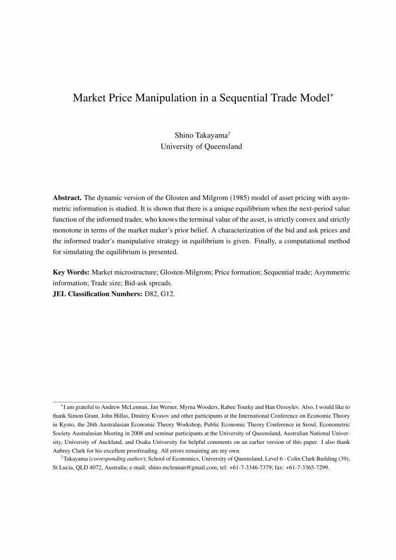
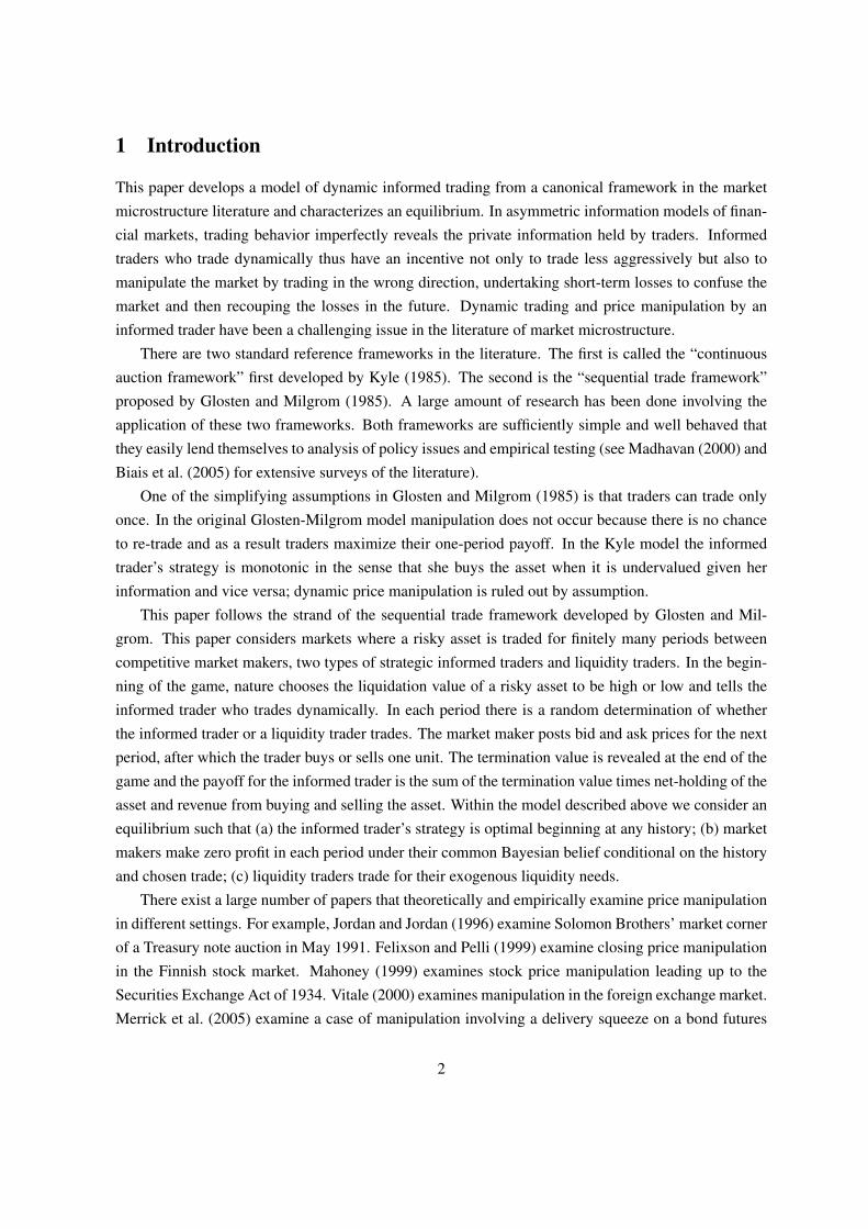
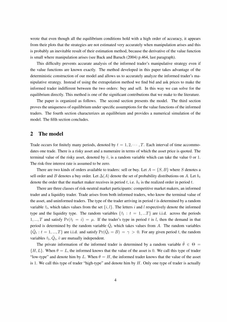
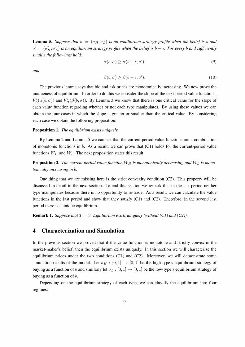
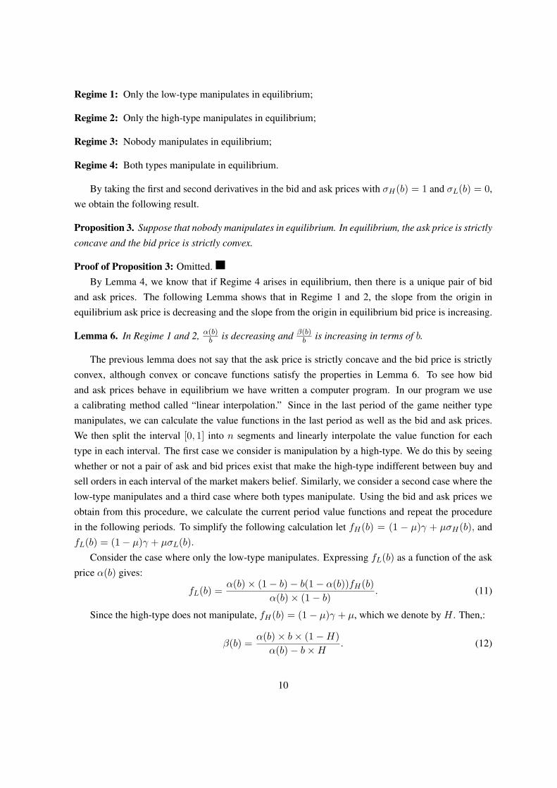
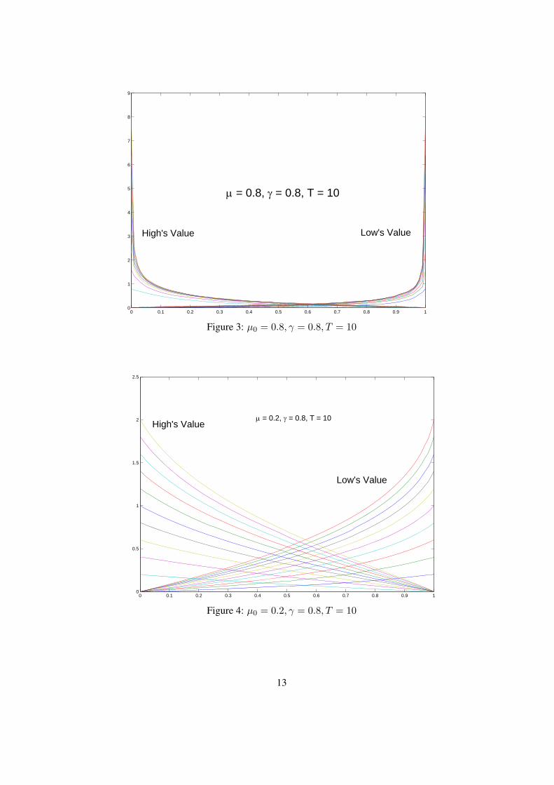
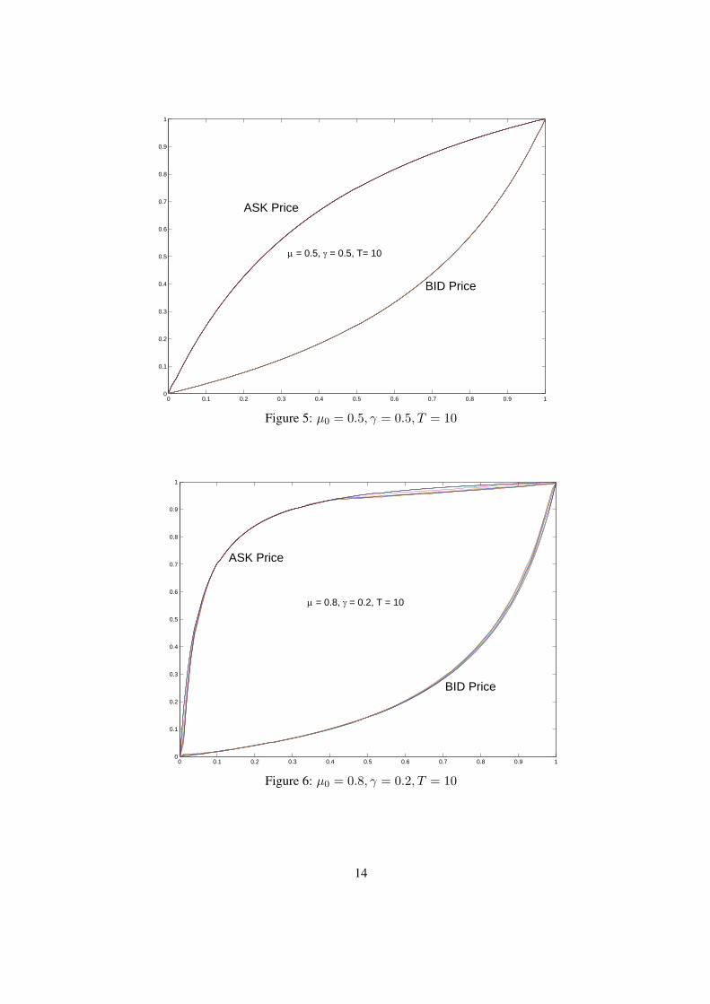
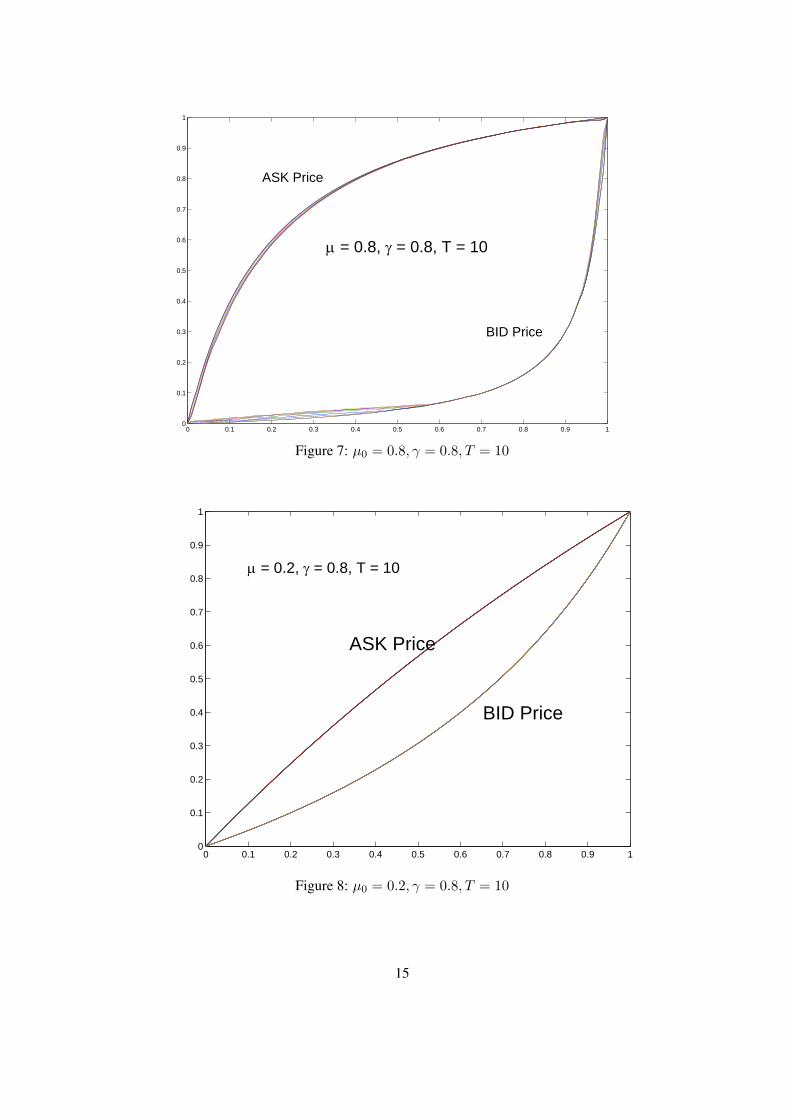
In our computer simulation we look for equilibrium pairs of bid and ask prices that satisfy theconditions for Regime 1 through 4. If there are two regimes, we ask the computer to report them. Then,we repeat this procedure recursively. The following figures describe the simulation results. Note thatwe have used a grid size of 100. Figures 1 to 4 show the value functions and figures 5 to 8 show theequilibrium prices.

In the figures of the bid and ask prices, there is a region of beliefs in which bid or ask pricesare different between periods. Given these beliefs, manipulation arises. Since the informed trader’sstrategy is different between the current period and the next period and so forth, bid or ask prices arealso different. The results of the simulation also show that the high-type manipulates in a region ofbeliefs close to 0 and the low-type manipulates in a region of beliefs close to 1. This result is somewhatcounter-intuitive, because for example if the high-type manipulates in a region of beliefs close to 0,bid price will be very low and he can only obtain a little amount of money. However, motivation formanipulation is to affect the future payoffs through market maker’s belief updating. Therefore, theywould manipulate when the bid and ask spread is small and the slope of the next-period value functionis steep.

11

0 0.1 0.2 0.3 0.4 0.5 0.6 0.7 0.8 0.9 10

0.5

1

1.5

2

2.5

3

3.5

4

4.5

5

High's ValueLow's Value

μ = 0.5, γ = 0.5, T = 10

Figure 1: µ0 = 0.5, γ = 0.5, T = 10

0 0.1 0.2 0.3 0.4 0.5 0.6 0.7 0.8 0.9 10

1

2

3

4

5

6

7

8

9

High's Value Low's Value

μ = 0.8, γ = 0.2, T = 10

Figure 2: µ0 = 0.8, γ = 0.2, T = 10

12

0 0.1 0.2 0.3 0.4 0.5 0.6 0.7 0.8 0.9 10

1

2

3

4

5

6

7

8

9

High's Value Low's Value

μ = 0.8, γ = 0.8, T = 10

Figure 3: µ0 = 0.8, γ = 0.8, T = 10

0 0.1 0.2 0.3 0.4 0.5 0.6 0.7 0.8 0.9 10

0.5

1

1.5

2

2.5

High's Value

Low's Value

μ = 0.2, γ = 0.8, T = 10

Figure 4: µ0 = 0.2, γ = 0.8, T = 10

13

0 0.1 0.2 0.3 0.4 0.5 0.6 0.7 0.8 0.9 10

0.1

0.2

0.3

0.4

0.5

0.6

0.7

0.8

0.9

1

ASK Price

BID Price

μ = 0.5, γ = 0.5, T= 10

Figure 5: µ0 = 0.5, γ = 0.5, T = 10

0 0.1 0.2 0.3 0.4 0.5 0.6 0.7 0.8 0.9 10

0.1

0.2

0.3

0.4

0.5

0.6

0.7

0.8

0.9

1

ASK Price

BID Price

μ = 0.8, γ = 0.2, T = 10

Figure 6: µ0 = 0.8, γ = 0.2, T = 10

14

0 0.1 0.2 0.3 0.4 0.5 0.6 0.7 0.8 0.9 10

0.1

0.2

0.3

0.4

0.5

0.6

0.7

0.8

0.9

1

ASK Price

BID Price

μ = 0.8, γ = 0.8, T = 10

Figure 7: µ0 = 0.8, γ = 0.8, T = 10

0 0.1 0.2 0.3 0.4 0.5 0.6 0.7 0.8 0.9 10

0.1

0.2

0.3

0.4

0.5

0.6

0.7

0.8

0.9

1

ASK Price

BID Price

μ = 0.2, γ = 0.8, T = 10

Figure 8: µ0 = 0.2, γ = 0.8, T = 10

15

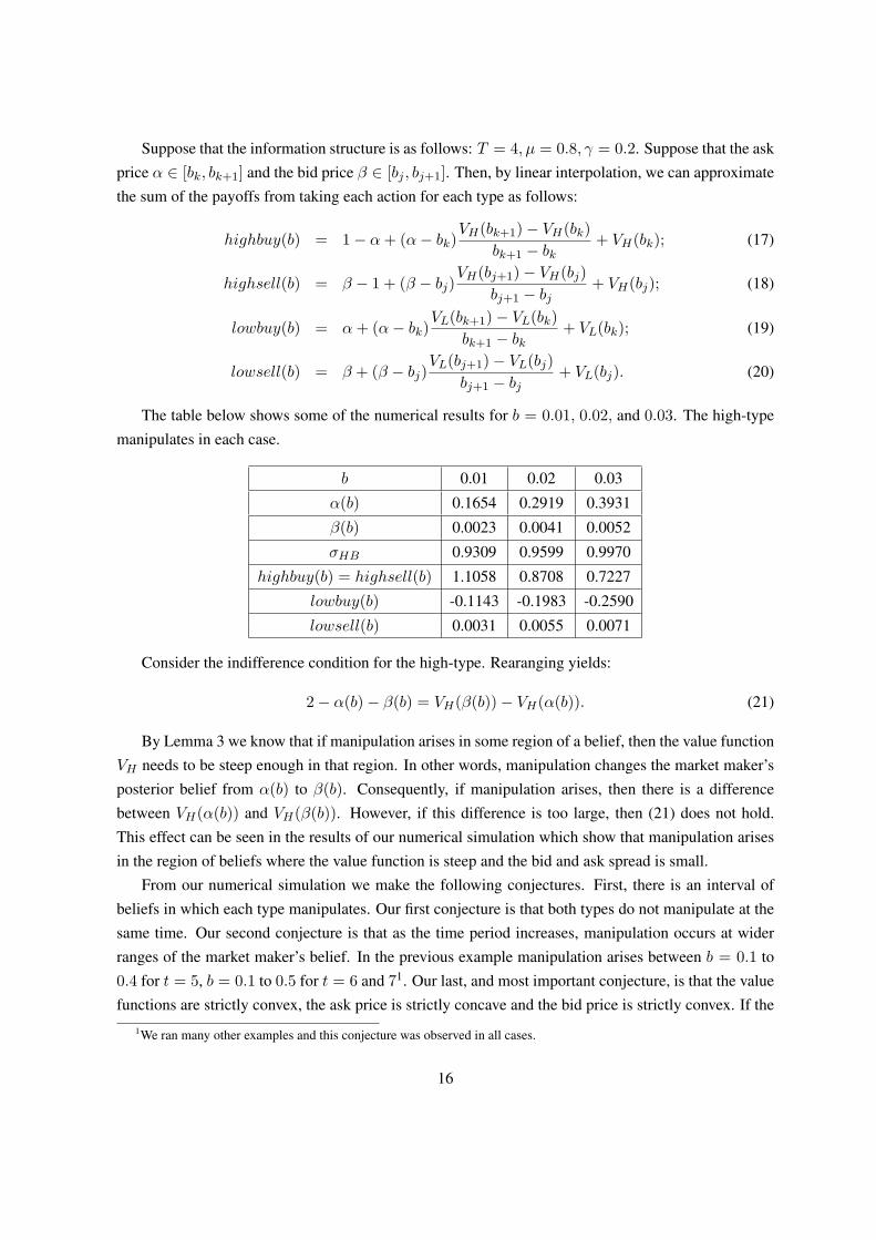
Suppose that the information structure is as follows: T = 4, µ = 0.8, γ = 0.2. Suppose that the askprice α ∈ [bk, bk+1] and the bid price β ∈ [bj , bj+1]. Then, by linear interpolation, we can approximatethe sum of the payoffs from taking each action for each type as follows:

highbuy(b) = 1− α+ (α− bk)VH(bk+1)− VH(bk)

bk+1 − bk+ VH(bk); (17)

highsell(b) = β − 1 + (β − bj)VH(bj+1)− VH(bj)

bj+1 − bj+ VH(bj); (18)

lowbuy(b) = α+ (α− bk)VL(bk+1)− VL(bk)

bk+1 − bk+ VL(bk); (19)

lowsell(b) = β + (β − bj)VL(bj+1)− VL(bj)

bj+1 − bj+ VL(bj). (20)

The table below shows some of the numerical results for b = 0.01, 0.02, and 0.03. The high-typemanipulates in each case.

b 0.01 0.02 0.03

α(b) 0.1654 0.2919 0.3931

β(b) 0.0023 0.0041 0.0052

σHB 0.9309 0.9599 0.9970

highbuy(b) = highsell(b) 1.1058 0.8708 0.7227

lowbuy(b) -0.1143 -0.1983 -0.2590

lowsell(b) 0.0031 0.0055 0.0071

Consider the indifference condition for the high-type. Rearanging yields:

2− α(b)− β(b) = VH(β(b))− VH(α(b)). (21)

By Lemma 3 we know that if manipulation arises in some region of a belief, then the value functionVH needs to be steep enough in that region. In other words, manipulation changes the market maker’sposterior belief from α(b) to β(b). Consequently, if manipulation arises, then there is a differencebetween VH(α(b)) and VH(β(b)). However, if this difference is too large, then (21) does not hold.This effect can be seen in the results of our numerical simulation which show that manipulation arisesin the region of beliefs where the value function is steep and the bid and ask spread is small.

From our numerical simulation we make the following conjectures. First, there is an interval ofbeliefs in which each type manipulates. Our first conjecture is that both types do not manipulate at thesame time. Our second conjecture is that as the time period increases, manipulation occurs at widerranges of the market maker’s belief. In the previous example manipulation arises between b = 0.1 to0.4 for t = 5, b = 0.1 to 0.5 for t = 6 and 71. Our last, and most important conjecture, is that the valuefunctions are strictly convex, the ask price is strictly concave and the bid price is strictly convex. If the

1We ran many other examples and this conjecture was observed in all cases.

16

third conjecture is proved, it would complete the proof of uniqueness result in a general case. To doso, proving the first conjecture would simplify the proof for a general case, because in this way we canfocus on one type.

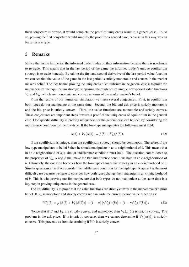
5 Remarks

Notice that in the last period the informed trader trades on their information because there is no chanceto re-trade. This means that in the last period of the game the informed trader’s unique equilibriumstrategy is to trade honestly. By taking the first and second derivative of the last-period value functionwe can see that the value of the game in the last period is strictly monotonic and convex in the marketmaker’s belief. The idea behind proving the uniqueness of equilibrium in the general case is to prove theuniqueness of the equilibrium strategy, supposing the existence of unique next-period value functionsVL and VH , which are monotonic and convex in terms of the market maker’s belief.

From the results of our numerical simulation we make several conjectures. First, in equilibriumboth types do not manipulate at the same time. Second, the bid and ask price is strictly monotonicand the bid price is strictly convex. Third, the value functions are monotonic and strictly convex.These conjectures are important steps towards a proof of the uniqueness of equilibrium in the generalcase. One specific difficulty in proving uniqueness for the general case can be seen by considering theindifference condition for the low-type. If the low-type manipulates the following must hold:

−α(b) + VL(α(b)) = β(b) + VL(β(b)). (22)

If the equilibrium is unique, then the equilibrium strategy should be continuous. Therefore, if thelow-type manipulates at belief b then he should manipulate in an ε-neighborhood of b. This means thatin an ε-neighborhood of b, a similar indifference condition must hold. The question comes down tothe properties of VL, α and β that make the two indifference conditions hold in an ε-neighborhood ofb. Ultimately, the question becomes how the low-type changes his strategy in an ε-neighborhood of b.Similar questions arise if we consider the indifference condition for the high type. Regime 4 is the mostdifficult case because we have to consider how both types change their strategies in an ε-neighborhoodof b. This is why proving our first conjecture that both types do not manipulate at the same time is akey step in proving uniqueness in the general case.

The last difficulty is to prove that the value functions are strictly convex in the market maker’s priorbelief. If VL is monotone and strictly convex we can write the current-period value function as:

WL(b) = µ (β(b) + VL(β(b))) + (1− µ) (γVL(α(b)) + (1− γ)VL(β(b))) . (23)

Notice that if β and VL are strictly convex and monotone, then VL(β(b)) is strictly convex. Theproblem is the ask price. If α is strictly concave, then we cannot determine if VL(α(b)) is strictlyconcave. This prevents us from determining if WL is strictly convex.

17

Proving the uniqueness of equilibrium in the general case is a challenging endeavor and this paperopens up the path to it. In this paper we have presented a model of dynamic informed trading, in whichthere exists a unique equilibrium under two conditions for the value functions. We have presented acomputational method to solve for an equilibrium and have made several conjectures for proving theuniqueness of equilibrium in the general case.

Appendix: Proof of Theorem 1

In order to prove the existence of equilibrium, we consider the equilibrium strategies (σ∗L, σ∗H) to be

a fixed point of the collection of their best response correspondences BR = {BRt}t=1··· ,T with BRt :[∆(A)]2 ⇒ [∆(A)]2 such that for each t, (σ∗L, σ

∗H) = BRt(σ∗L, σ

∗H). Let U tn : ∆(A) × [0, 1]2 → IR

denote the payoff function for the type n ∈ N trader in period t. More formally, for n ∈ {H,L},

U tn(σn, pt) =T∑t′=t

[σnB(θ − αt′)− σnS(θ − βt′)] . (24)

Then, we define the informed trader’s best response correspondence: for every t ∈ {1, · · · , T} andgiven pt,

BRt(σL, σH) ={

(σL, σH) ∈ [∆(A)]2|σn ∈ arg maxσ∈∆(A)

U tn(σ, pt) ∀n ∈ N}. (25)

Therefore, when b(ht) = bt, α∗t (b(ht)) = αt and β∗t (b(ht)) = βt, continuation value of the gamefor the high-type in period t is:

V tH(bt) = max

σH∈∆(A)[σHB(1− αt + V t+1

H (b(ht, B))) + σHS(βt − 1 + V t+1H (b(ht, S)))], (26)

and one for the low type is:

V tL(bt) = max

σL∈∆(A)[−σLBαt + V t+1

L (b(ht, B)) + σLS(βt + V t+1L (b(ht, S)))]. (27)

Thus, an equilibrium defined in Definition 3 is a fixed point of the best response correspondenceBR, and αt and βt are respectively updated by Bayes rule.

Lemma 8. The payoff function U tn is continuous. In addition, for every t, BRt is a upper semi-continuous correspondence.

Proof: Since the argument is symmetric, we only consider the high-type’s payoff function and thevalue function. Note that U tH is continuous in his strategy and also the market maker’s quotes (βt, αt).Then, U tH is a continuous numerical function.

We respectively denote the sequences of prices associated with σk and σk by pk and pk and also σand σ by p and p. Then, since the prices are continuous in strategies, we have pk → p and pk → p.

18

Now on the contrary, suppose that there exists a sequence as above but σ /∈ BR(σH , σL). Withoutloss of generality, we suppose that there exists a ε > 0 and σH ∈ ∆(E) such that:

U tH(σH , p) > U tH(σH , p) + 3ε. (28)

For k large enough, by continuity of the payoff function and prices, we have:

U tH(σH , pk) > U tH(σH , p)− ε > U tH(σH , p) + 2ε

> U tH(σkH , p) + ε > U tH(σkH , pk). (29)

This contradicts with the fact that (σkH , σkL) ∈ BRt(σkH , σkL) for all k.

Lemma 9. The set [∆(A)]2 is non-empty, compact and convex.

Proof: The set of strategies ∆(A) is non-empty, compact and convex. The set [∆(A)]2 is a Cartesianproduct of those sets and thus the result follows.

Lemma 10. The informed trader’s best response correspondenceBRt is non-empty and convex-valuedfor every t ∈ {1, · · · , T}.

Proof: We will prove this by mathematical induction. Since the argument is symmetric, we onlyconsider the high type. Consider the last period t = T . Then, the high type and low type trade on theirinformation. In this sense,BRT is non-empty and convex-valued. Next we suppose that in period t+1,BRt+1 is non-empty and convex-valued. Then, we will prove that in period t, BRt is also non-emptyand convex-valued.

By the assumption for the inductive hypothesis, we know that V t+1H is well-defined. Now, fix a

history ht−1 arbitrarily. Then, given V t+1H , the right hand side of the expression in (26) is linear in the

strategies σH . Therefore the expression in (26) has a maximum so that the set BRt is non-empty.Second, we will prove that it is also convex-valued. Take two different strategies (σH , σL) ∈

BRt(σH , σL) and (¯σH , σL) ∈ BRt(σH , σL). We denote the prices associated with the strategies(σH , σL) by pt. Then, the following must hold: U tH(σH , pt) = U tH(¯σH , pt).

Let σtH = γσH + (1 − γ)¯σH for some γ ∈ (0, 1). By using linearity of the payoff function, weconclude: (σH , σL) ∈ BRt(σH , σL). Therefore, BRt is convex-valued.

Proof of Theorem 1: By Lemma 8 to Lemma 10, we can apply the Kakutani’s fixed point theorem tothe best response correspondence BRt on [∆(A)]2 for all t ∈ {1, · · · , T}.

Appendix: Proofs

Proof of Lemma 1 - 1: On the contrary, suppose that for some b, bid-ask spread is negative. That is,

19

α(b, σ) ≤ β(b, σ). Then, we have:

1− α(b, σ) + VH(α(b, σ)) > β(b, σ)− 1 + VH(β(b, σ)); (30)

−α(b, σ) + VL(α(b, σ)) < β(b, σ) + VL(β(b, σ)). (31)

Then, it must be the case that in equilibrium σHB = 1 and σLB = 0. Then, by the Bayes rule, wehave:

α(b, σ) > b > β(b, σ), (32)

which contradicts with our assumption. �

Proof of Lemma 1 - 2: The result follows from 1 and Bayes rule. �

Proof of Lemma 4: We define J(α, β) ≡

(H(α, β)L(α, β)

)where for α ∈ [0, 1] and β ∈ [0, 1],

H(α, β) = VH(α)− VH(β) + 2− α− β, (33)

andL(α, β) = VL(α)− VL(β)− α− β. (34)

Since VH is a decreasing function and VL is a increasing function and by Lemma 3, the determinantof J denoted by J satisfies:

J (α, β) = −[V ′H(α)− 1]× [V ′L(β) + 1] + [V ′H(β) + 1]× [V ′L(α)− 1] > 0. (35)

Since the elements in the upper left corner of J and the lower right corner of J are both strictlynegative, we conclude that J is negative definite. Take two distinct p1 = (α1, β1) and p2 = (α2, β2).Therefore, we have: J (p1) 6= J (p2). Finally, we conclude that there exists only one pair of α and βwhich satisfies: H(α, β) = 0 and L(α, β) = 0.

Proof of Lemma 5: When nobody manipulates, by the Bayes rule we can show that bid and ask pricesdecrease as market makers’ belief b decreases. By Lemma 4, there are no two distinct pairs of bid andask prices at which both types manipulate. Now, we suppose that only one type manipulates. Since theargument is symmetric, suppose that the low-type manipulates at b. Then, we have:

−α(b, σ) + VL(α(b, σ)) = β(b, σ) + VL(β(b, σ)); (36)

−α(b− ε, σ′) + VL(α(b− ε, σ′)) ≤ β(b− ε, σ′) + VL(β(b− ε, σ′)). (37)

Then, we obtain:

(α(b, σ)− α(b− ε, σ′))(VL(α(b− ε, σ′))− VL(α(b, σ))α(b− ε, σ′)− α(b, σ)

− 1)

≥ (β(b, σ)− β(b− ε, σ′))(1 +VL(β(b, σ))− VL(β(b− ε, σ′)

β(b, σ)− β(b− ε, σ′)). (38)

20

By Lemma 3 and Lemma 4, we can see that bid and ask prices move in the same direction, whichis impossible when only the low-type manipulates.

Lemma 11. Suppose that in equilibrium one type takes a manipulative strategy and the other type doesnot. Then, the equilibrium strategy exists uniquely.

Proof of Lemma 11: Since the argument is symmetric, we will prove the result for the case where onlythe high-type manipulates. We will show that given b and σL there is a unique pair of strategies σHsatisfying the condition that the high-type is indifferent between buy and sell. On the contrary, supposethat there are different strategies σH satisfying the indifference condition for the high-type with theprices α(b, σ) and β(b, σ). Now, suppose that: σHB < σHB ≤ 1. Then, we have: α(b, σ) > α(b, σ)and β(b, σ) < β(b, σ). Then, we have:

1− α(b, σ) + VH(α(b, σ)) ≥ β(b, σ)− 1 + VH(β(b, σ)). (39)

Thus, we have:

α(b, σ)−α(b, σ)−VH(α(b, σ))+VH(α(b, σ)) ≤ β(b, σ)−β(b, σ)+VH(β(b, σ))−VH(β(b, σ)). (40)

By Lemma 3, we have:

β(b, σ)− β(b, σ) + VH(β(b, σ))− VH(β(b, σ)) < 0. (41)

However, since VH is decreasing, the left hand side of (40) is strictly greater than 0, which makes40 impossible to hold.

Lemma 12. If the equilibrium bid and ask prices are unique at b, the equilibrium strategies are unique.

Proof of Lemma 12: For the simplicity of notation, let fH = (1−µ)γ +µσHB and fL = (1−µ)γ +µσLB. Suppose that in equilibrium, there are two different pairs of strategies, σ and σ. Now on thecontrary, suppose that α(b, σ) = α(b, σ) and β(b, σ) = β(b, σ). Similarly with fH and fL, we definefH and fL associated with σLB and σHB . By the Bayes rule, we can write: α(b, σ) = fHb

fHb+(1−b)fL,

and α(b, σ) = fHb

fHb+(1−b)fL. Since α(b, σ) = α(b, σ), we must have:

fHfL = fLfH . (42)

Similarly, we have β(b, σ) = (1−fH)b(1−fH)b+(1−b)(1−fL) , and β(b, σ) = (1−fH)b

(1−fH)b+(1−b)(1−fL). By equat-

ing them, we must have:(1− fH)(1− fL) = (1− fL)(1− fH). (43)

Combining the equations (42) and (43) gives fH − fH = fL − fL ≡ ∆. Then, by substituting itinto (42) we obtain:

(fH + ∆)fL = (fL + ∆)fH . (44)

21

Therefore, we must have fH = fL and fH = fL. Conversely, if fH = fL and fH = fL, thenβ(b, σ) = β(b, σ) = b and α(b, σ) = α(b, σ) = b. This contradicts with Lemma 1.

Proof of Proposition 1:Case 1: V ′L(α(b, σ)) > 1 and V ′H(β(b, σ)) < −1In this case, both types could either manipulate or not manipulate in equilibrium. By Lemma 11, if oneof the two types manipulates and the other does not, there exists a unique equilibrium. It remains toshow that one equilibrium in which both do not manipulate does not co-exist with the other equilibriumin which both manipulate.

Call a non-manipulative equilibrium strategy σ and a manipulative equilibrium strategy σ. Then,we have: α(b, σ) < α(b, σ) and β(b, σ) > β(b, σ).

Then, for the high-type, we have:

1− α(b, σ) + VH(α(b, σ)) = β(b, σ)− 1 + VH(β(b, σ)), (45)

and1− α(b, σ) + VH(α(b, σ)) > β(b, σ)− 1 + VH(β(b, σ)). (46)

Similarly, for the low-type, we have:

−α(b, σ) + VL(α(b, σ)) = β(b, σ) + VL(β(b, σ)), (47)

and−α(b, σ) + VL(α(b, σ)) < β(b, σ) + VL(β(b, σ)). (48)

Thus, we must have:

VL(β(b, σ))− VL(β(b, σ))− [VL(α(b, σ))− VL(α(b, σ))]

> −α(b, σ) + α(b, σ)− [β(b, σ)− β(b, σ)]

> VH(β(b, σ))− VH(β(b, σ))− [VH(α(b, σ))− VH(α(b, σ))]. (49)

Since α(b, σ) < α(b, σ), β(b, σ) > β(b, σ), VH is decreasing and VL is increasing, the inequality(49) is impossible. This complete our proof in this case. �

Case 2: V ′L(α(b, σ)) > 1 and V ′H(β(b, σ)) ≥ −1In this case, the high-type does not manipulate. The low-type either manipulate or does not. The proofis done by Lemma 11. �

Case 3: V ′L(α(b, σ)) ≤ 1 and V ′H(β(b, σ)) < −1In this case, the high-type does not manipulate. The low-type either manipulate or does not. Similarlywith Case 2, the proof is done by Lemma 11. �

Case 4: V ′L(α(b, σ)) ≤ 1 and V ′H(β(b, σ)) ≥ −1In this case, both types do not manipulate and therefore, the equilibrium exists uniquely. �

22

In the end, we conclude that equilibrium exists uniquely in every case.

Proof of Proposition 2:·When t = T

Since this is the last chance to trade, both types trade on their information. Therefore,

WH(b) = (1− [µ+ (1− µ)γ]b(1− µ)γ + µb

) · µ =(1− b)(1− µ)γ(1− µ)γ + µb

· µ. (50)

Therefore, we conclude that WH is strictly decreasing in b. �

·When t = 1, · · · , T − 1By Lemma ??, equilibrium exists uniquely. Let b > b′, and σ′ denotes the equilibrium strategy whenthe belief is b′. Then, we have:

WH(b) = µ (1− α(b, σ) + VH(α(b, σ))) + (1− µ) (γVH(α(b, σ)) + (1− γ)VH(β(b, σ)))

< µ(1− α(b′, σ′) + VH(α(b′, σ′))

)+ (1− µ)

(γVH(α(b′, σ′)) + (1− γ)VH(β(b′, σ′))

)= WH(b′).

This completes our proof.

Let: P (b) = fH(b)× b+ fL(b)× (1− b).

Lemma 13. Fix a history ht arbitrarily and suppose that b = b(ht). Suppose that VH is monotonicallydecreasing and strictly convex in the market maker’s prior b and that VL is monotonically increasingand strictly convex in b. Suppose that only one type manipulates at the belief b. Then, P is increasingat the belief b.

Proof of Lemma 13:Case 1: When the high-type manipulates at the belief b.By the indifference condition, we know that if the high-type manipulates, then the slope between bidand ask prices should be:

dH(b) =α(b) + β(b)− 2α(b)− β(b)

. (51)

Thus, we obtain:

d′H(b) =α′(b)(1− β(b))− β′(b)(1− α(b))

[α(b)− β(b)]2× 2. (52)

Suppose that the high-type manipulates at the belief b. Then by the continuity of the equilibriumstrategy, we must have d′H(b) > 0 because the equilibrium strategy is unique. By the Bayes rule, wehave:

log(1− α(b)) = log(1− b) + log(1− µ)γ − logP (b), (53)

23

andlog(1− β(b)) = log(1− b) + log((1− µ)(1− γ) + µ)− log(1− P (b)). (54)

By taking the first derivative of the above equations, we obtain:

−α′(b)1− α(b)

=−1

1− b− P ′(b)P (b)

, (55)

and−β′(b)

1− β(b)=−1

1− b+

P ′(b)1− P (b)

. (56)

Notice that:

α′(b)(1− β(b))− β′(b)(1− α(b)) = (1− α(b))(1− β(b))× P ′(b)×(

1P (b)

+1

1− P (b)

).

Therefore, we have:

d′H(b) =(1− α(b))(1− β(b))× P ′(b)×

(1

P (b) + 11−P (b)

)[α(b)− β(b)]2

× 2. (57)

and thus we conclude P ′(b) > 0. �

Case 2: When the low-type manipulates at the belief b.By the indifference condition, we know that if the low-type manipulates, then the slope between bidand ask prices should be:

dL(b) =α(b) + β(b)α(b)− β(b)

. (58)

Thus, we obtain:

d′L(b) =α(b)β′(b)− α′(b)β(b)

[α(b)− β(b)]2× 2. (59)

Suppose that the low-type manipulates at the belief b. Then by the continuity of the equilibriumstrategy, we must have d′L(b) > 0 because the equilibrium strategy is unique. By the Bayes rule, wehave:

logα(b) = log b+ log((1− µ)γ + µ)− logP (b), (60)

andlog β(b) = log b+ log(1− µ)(1− γ)− log(1− P (b)). (61)

By taking the first derivative of the above equations, we obtain:

α′(b)α(b)

=1b− P ′(b)P (b)

, (62)

andβ′(b)β(b)

=1b

+P ′(b)

1− P (b). (63)

24

Notice that:

α(b)β′(b)− α′(b)β(b) = α(b)β(b)× P ′(b)×(

11− P (b)

+1

P (b)

). (64)

Thus, we can write:

d′L(b) =α(b)β(b)× P ′(b)×

(1

1−P (b) + 1P (b)

)[α(b)− β(b)]2

× 2. (65)

Thus, we must have P ′(b) > 0.

Proof of Lemma 6:Regime 1: By the Bayes rule, we have:

b× ((1− µ)γ + µ) = P (b)× α(b), (66)

andb(1− µ)(1− γ) = (1− P (b))× β(b). (67)

By Lemma 13, for k < 1, we have:

P (b)P (kb)

=α(kb)kα(b)

> 1, (68)

and1− P (b)1− P (kb)

=β(kb)kβ(b)

< 1. (69)

Dividing both sides by b and arranging terms yields the desired results. �

Regime 2: The proof will be done in a similar fashion with the previous lemma. �

Appendix: Numerical Simulation

Let mHk = VH(bk+1)−VH(bk)

bk+1−bk and mHj = VH(bj+1)−VH(bj)

(bj+1−bj) . Moreover, let (1− µ)(1− γ) + µ = L.

Lemma 14. When the high-type manipulates, then equilibrium ask price αH solves:

(mHk − 1)α2

H + αH(−bkmH

k + 1 + VH(bk) + (b+ L(1− b))(1−mHk ))

+αH[L(1− b) + [bj − 1 + L(1− b)]mH

j − VH(bj)]

−(−bkmHk + 1 + VH(bk))(b+ L(1− b))

+(−L(1− b) + [b(1− bj)− bjL(1− b)]mHj + VH(bj) (b+ L(1− b)) = 0. (70)

Moreover, equilibrium ask price αH must satisfy:

H ≡ α(1− L)(1− b)b(1− α)

≤ (1− µ)γ + µ. (71)

25

Proof of Lemma 14: To avoid lengthy calculations, we only explain the key steps. Then, the equationin question is:

1−α+(α−bk)mHk +VH(bk) =

(b− α) + αL(1− b)(b− α) + L(1− b)

−1+((b− α) + αL(1− b)(b− α) + L(1− b)

−bj)mHj +VH(bj).

It is very similarly done with Lemma 7. Finally, we obtain the desired result.

Let mDk = D(bk+1)−D(bk)

bk+1−bk and mDj = D(bj+1)−D(bj)

bj+1−bj .

Lemma 15. If both types manipulate, then the equilibrium ask price αM and strategy σ∗HB satisfies:

mDk α

2M + αM

[−bkmD

k +D(bk)− bH∗mDk + (b(H∗ − 1) + bj)mD

j − (D(bj) + 2)]

+ bH∗(D(bj) + 2− bjmDj + bkm

Dk −D(bk)) = 0, (72)

andH∗ = (1− µ)γ + µσ∗HB. (73)

Proof of Lemma 15: For the simplicity of notation, let us define: D = VL − VH . If both typesmanipulate, this means that there is a pair of ask and bid prices which satisfies: D(α) = D(β) + 2.By using the linear interpolating method, we check if there is a pair of α, b and H which satisfies theindifference conditions for both types:

(α− bk)mDk +D(bk) =

[αb(H − 1)(bH − α)

− bj]mDj +D(bj) + 2. (74)

Then, we obtain the desired result.

References

Aggarwal, R., Wu, G. (2006). Stock market manipulations - theory and evidence. Journal of Business,79:1915–1953.

Allen, F., Gale, D. (1992). Stock price manipulation. Review of Financial Studies, 5:503—529.

Allen, F., Gorton, G. (1992). Stock price manipulation, market microstructure and asymmetric infor-mation. European Economic Review, 36:624—630.

Back, K., Baruch, S. (2004). Information in securities markets: Kyle meets Glosten and Milgrom.Econometrica, 72:433–465.

Back, K., Baruch, S. (2007). Working orders in limit-order markets and floor exchanges. The Journalof Finance, 61:1589–1621.

26

Biais, B., Glosten, G., Spatt, C. (2005). Market microstructure: a survey of microfoundations, empiricalresults, and policy implications. Journal of Financial Markets, 8:217–264.

Boulatov, A., Kyle, A., Livdan, D. (2005). Uniqueness of equilibrium in the single-period Kyle’85Model. Working Paper.

Brunnermeier, M. K., Pedersen, L. H. (2005). Predatory trading. The Journal of Finance, LX:1825–1864.

Chakraborty, A., Yilmaz, B. (2004). Informed manipulation. Journal of Economic Theory, 114:132–152.

Felixson, K., Pelli, A. (1999). Day end returns – stock price manipulation. Journal of MultinationalFinancial Management, 9:95–127.

Glosten, L. R., Milgrom, P. R. (1985). Bid, ask and transaction prices in a specialist market withheterogeneously informed traders. Journal of Financial Economics, 14:71–100.

Huberman, G., Stanzl, W. (2004). Price manipulation and quasi-arbitrage. Econometrica, 72:1247–1275.

Jordan, B. D., Jordan, S. D. (1996). Solomon brothers and the may 1991 treasury auction: Analysis ofa market corner. Journal of Banking and Finance, 20:25–40.

Kyle, A. S. (1985). Continuous auctions and insider trading. Econometrica, 53:1315–1336.

Madhavan, A. (2000). Market microstructure: a survey. Journal of Financial Markets, 3:205–258.

Mahoney, P. G. (1999). The stock pools and the securities exchange act. Journal of Financial Eco-nomics, 51:343–369.

Merrick, J. J., Narayan, Y. N., Yadav, K. P. (2005). Strategic trading behavior and price distortion in amanipulated market: Anatomy of a squeeze. Journal of Financial Economics, 77:171–218.

Vitale, P. (2000). Speculative noise trading and manipulation in the foreign exchange market. Journalof International Money and Finance, 19:689–712.

27