Embed Size (px)
Citation preview
Market Making in the
Interbank Foreign Exchange Market
Jian Yao
First Draft: November 15, 1996This Draft: November 2, 1997
CorrespondenceJ.P. Morgan Investment Management Inc.522 Fifth AvenueNew York, NY 10036Tel: (212)837-2711, Fax: (212)944-2371Email: [email protected]
This paper is a revised version of chapter one of my Ph.D. dissertation at New York University. Iwish to thank members of my dissertation committee, Joel Hasbrouck (co-chair), Richard Levich(co-chair) and Matthew Richardson, for their guidance and encouragement. I also benefited fromcomments and suggestions made by Jose Campa, Edwin Elton, Martin Gruber, Jianping Mei,William Silber and participants at NYU finance seminar. I am grateful to Heinz Riehl, DavidBuchen and a major commercial bank in New York City for providing the foreign exchangedealing data used in this study. All errors are entirely my own.

Abstract
This paper studies the market making behavior of FX dealers in the interbank market which ischaracterized by high trade volume and decentralized market structure. The dataset for myempirical estimation is based on the complete trade records of a FX dealer at a major commercialbank over 25 trading days. The dealer is among the five largest DM/$ dealers in the world, and thecomposition of his trades (customer trades, inter-dealer trades, etc.) is representative of the industry.
I find evidence that incoming trades have information effects. However, I do not find evidenceof price-shading as a tool for inventory control in inter-dealer trades. This is consistent with theview that quote shading signals a dealer’s position, and further reveals information from hisproprietary order flows. A representative FX dealer instead lays off most undesired inventoriesthrough outgoing trades against other dealers’ quotes. Price impacts of such outgoing trades areminimized because the depth and low transparency of this market, together with the electronicdealing systems, allow a dealer to search effectively for the best prices. A dynamic analysisindicates that large trades have significant lagged price impacts, and that FX dealer oftenstrategically delays quote revision to take advantage of low market transparency while working offinventory shocks. My study also suggests that dealers with diverse market positions might preferdifferent trading strategies. For example, an uninformed dealer with little customer business islikely to shade quotes for inventory control.
1
1. Introduction
Foreign exchange (FX) markets are characterized by short-term price fluctuations which
researchers in international finance have long agreed can not be explained by long-term
economic fundamentals. However, little research has been done to study the question of how
trading mechanisms in FX markets affect the price formation process at the market
microstructure level. The interbank FX market is of great interest in particular because it is the
world's most active financial market and because it is where most FX trading takes place1.
Moreover, the interbank market is unique because of its largely unregulated and decentralized
dealership market structure.
This paper studies the market making behavior of FX dealers who are subject to adverse
selection arising from private information, and who have to manage inventory shocks from order
flows. A unique dataset of complete trade records of one of the most active $/DM dealers in the
interbank market allows me to address several market microstructure hypotheses. Because the
interbank FX market is basically unregulated and free from market friction such as high liquidity
costs, this paper focuses on the dealer’s inventory management behavior in the presence of
traders with heterogeneous information. Since I have all the information on each trade of this
dealer, I can examine the dealer’s market making behavior testing whether he takes advantage of
the low order transparency in the FX market. In particular, I study the transient versus persistent
price impacts from order flows, as well as the dealer’s joint management of inventory shocks and
information impacts. Using data on trade counterparty identity, I examine different types of
1 According to Bank of International Settlements 1996 survey, global foreign exchange turnover reached a dailyaverage of $1.2 trillion in April 1995, an increase of 45% from 1992. The US market alone had a daily turnover of$244 billion in April 1995. To put this number in perspective, Frankel and Froot (1990) estimate that the annualizedFX turnover in US market alone in 1989 equals about twice world GDP. On the other hand, trade volume on FXfutures market is only a small percentage of that on the spot market. For example, Lyons (1995) estimates that in

2
trades (such as customer versus inter-dealer trades) and provide insights into the dealer’s
strategic behavior under different circumstances as the dealer attempts to optimize inventory
control and protection against adverse selection.2
The most comparable study of FX dealer behavior in the literature is Lyons (1995), which
represents the first attempt to use proprietary dealer inventory and trade data. However, Lyons’
results are limited by certain aspects of his dataset. The most significant limitation is that there is
no customer trade data in his 5-day sample. Customer trades are important because they are the
major source of private information in the FX market. As a result, his study focuses primarily on
incoming inter-dealer trades, and fails to address a broader range of issues such as the possibility
of different strategies for customer and inter-dealer trades. In contrast, the dataset in this study
comprises the complete trading records of a major market maker at one of the five largest $/DM
dealing banks. The dealer has substantial customer flows over the entire 25-day sample period.
Most importantly, the composition of his trades (customer trades, direct and brokered inter-dealer
trades, etc.) is representative of the industry as depicted in market-wide surveys by the Bank of
International Settlements (1993, 1996). Because of the dealer’s status as a major market maker and
of the representative composition of his trades, his activities offer a reasonable proxy for market
making activities in the FX market. The complete records of his dealing activities thus allow me to
examine market microstructure issues with respect to some of the most unique and interesting
aspects of this market.
1992 the average daily volume on all IMM $/DM contracts was less than $5 billion, one tenth of the daily spotvolume in the U.S. during the same period.2 Yao (1997) further exploits the dataset to examine FX dealer trading profits from different sources and marketmaking costs. One interesting finding is that although customer trades account for less than 14% of the dealer’s totaltrade volume, they represent about 75% of his total profits over the 25-day sample period.

3
There are three major findings in this paper along with some other results. First, there is
little evidence of quote-shading (raising quotes when the dealer is short relative to his desired
position and lowering quotes when he is long) as a tool for inventory control in inter-dealer trades.
This is consistent with the view that quote shading signals a dealer’s position to other dealers, and
further reveals information from his proprietary order flows. Because the concern of revealing
information which the counterparty can capitalize on is mitigated in customer trades, data suggests
that the dealer in my study shades prices quoted to customers. Second, I find that instead of shading
quotes in hope of eliciting trades of a desired sign, the FX dealer lays off most inventory shocks
through outgoing trades by hitting other dealers’ quotes. The high liquidity, tight spreads3 and low
transparency of the FX interbank market, together with the electronic dealing systems, allow a
dealer to search effectively for the best prices for his outgoing trades and hence minimize price
impacts. Third, while incoming trades have information effects in general, large trades have
particularly significant lagged price impacts. A dynamic analysis indicates that the FX dealer often
strategically delays quote revision subsequent to incoming trades to take advantage of low market
transparency while working off inventory shocks.
The paper is organized as follows: Section 2 briefly reviews the literature on market
microstructure and its application to foreign exchange markets. Section 3 develops an integrated
framework for studying the price impact from the dealer’s incoming and outgoing trades. Section
4 describes the data and reports some descriptive statistics. Section 5 discusses the test
3 For $/DM, a bid-ask spread of 3 - 5 pips is typical for transactions less than $20 million (the mean and mediantransaction size in my sample is $8.4 million), where 1 pip, the smallest increment in quotes, equals one hundredth ofa pfennig, or 0.0001 DM versus US dollar. This amounts to only about 0.02 - 0.04% of transaction price. Using dailyclosing quotes from Reuters, Bessembinder (1994) reports that mean spot FX spreads range from 0.049% for $/DMto 0.079% for $/SF. By comparison, Amihud and Mendelson (1986) report spreads for NYSE stock portfoliosranging from .5% to 3.2%, and Stoll (1989) reports that spreads for OTC stocks range from 1.2% for the largestdecile to 6.9% for the smallest decile.

4
specifications and empirical methods, and presents the results of model estimation. Section 6
provides a dynamic VAR analysis of price, trade and inventory. Finally section 7 concludes.
2. Literature Overview
The literature on market microstructure is well developed as it pertains to the centralized
market structure of NYSE specialists. There are two principal approaches to modeling market
making behavior. First, inventory control models (e.g. Garman, 1976; Amihud and Mendelson,
1980; O’Hara and Oldfield, 1986; among others) consider the pricing problem faced by risk-
averse dealers to keep their inventories within bounds. For specialists, the only tool is to adjust
price, or shade quotes, to offset order flow fluctuations. Ho and Stoll (1983) extend the study of
dealer pricing-setting to markets with multiple dealers. Second, asymmetric information models
(e.g. Glosten and Milgrom, 1985; Admati and Pfleiderer, 1988; among others) focus on adverse
selection problems when there are traders with heterogeneous information. In these models,
dealers set spreads to guard against informed traders, and update their own price expectations
from trades. In reality, dealers are likely to confront both problems. However, since both models
predict that buyer-initiated trades push up prices and seller-initiated trades push them down,
disentangling the two effects presents a challenge to empirical studies. Hasbrouck (1988)
suggests that the two effects can be separated through dynamic analyses. The inventory control
component of price change is transient while the information component is permanent, reflecting
the impounded new information. Madhavan and Smidt (1991, 1993) develop theoretical models
that incorporate both effects and test them using inventory and trade data. The earlier (1991)
paper analyzes intraday trades and finds that price changes reflect significant information effects
but weak inventory control effects.

5
Extending the theoretical models of centralized specialist markets to FX market poses the
challenge of modeling a decentralized, multiple-dealer environment with such additional features
as low market transparency. Among the few attempts, Lyons (1996) provides a model of risk-
averse FX dealers who prefer ex-ante low market transparency because it gives them time to
manage inventories and reduce market-making risk inherent in price discovery . Although not
related directly to the FX market, a multi-period, multiple-dealer model developed by Hansch,
Naik and Viswanathan (1993) posits that relative inventory differences determine dealer
behavior. Their model is supported by tests using London Stock Exchange (a dealership market)
data and provides useful implications for FX market microstructure studies.
As for empirical work on FX market microstructure, efforts are hampered by the
difficulty in obtaining detailed data. Dealers’ inventory and trade data are proprietary information
of their respective banks, and are not generally available to the public. Recently a body of
research on FX market microstructure has emerged using Reuters indicative quotes. The research
focuses mostly on dealer bid-ask spreads (e.g. Huang and Masulis,1995) and FX price volatilities
(e.g. Anderson and Bollerslev,1996). Since indicative quotes from Reuters screens are not
transaction prices and do not provide any measure of order flow, these studies fail to address FX
dealer market making behavior directly. In a study of dealer inventories and spreads,
Bessembinder (1994) finds that FX spreads increase with forecasts of price risk, with interest
rates, and before weekends. Although these results are consistent with an inventory cost model,
the study provides no insight on intraday inventory swings and quote adjustments because it uses
only daily closing quotes.
Lyons (1995) is the first study that utilizes dealer intraday inventory and trade data in FX
markets. His data supports both asymmetric information and inventory control models. However,

6
generalization of his findings is subject to questions because of the following two aspects of his
data. First, his dataset spans only 5 trading days (August 3-7, 1992), and it is not clear whether
these days or the dealer are representative of the overall FX market. Second, during those 5
trading days, there are virtually no customer trades in the sample. Customer trades are important
in the FX market because they represent the major source of asymmetric information, and
because they often generate a significant portion of dealer profits.
This paper studies the market making behavior of a representative FX dealer who is a
major player in the market and whose trade composition (customer flows, inter-dealer trades,
etc.) is representative of the industry. The study uncovers unique dealer behavior arising from the
interbank FX market’s tremendous trade volume and liquidity, as well as its decentralized
market structure.
3. The Model
I start with some institutional background of the interbank FX market, which is essential
to the model below. Figure 1 outlines the two major types of transactions in this market,
customer-dealer trades and inter-dealer trades, as well as the major channels through which these
trades are conducted.
Figure 1 Here
Although customer trades account for only 10 - 15% of total trade volume in the inter-
bank FX market, dealers emphasize the importance of customer trades because without them
their view and understanding of the market will be limited. Moreover, customer trades generate
the majority of trading profits for most FX dealers. In this market, each FX dealer has a different
7
level of access to customers, who trade with dealers through banks’ sales staff4. Because of lack
of trade reporting requirement, a FX dealer has no direct information about other dealers’
customer trades. Therefore, knowledge of customer order flow is a major source of asymmetric
information in the interbank FX market.
In inter-dealer trades, a FX dealer lays off inventory shocks from customer trades. In the
meantime, he also provides liquidity to other dealers. Inter-dealer trades are conducted through
either brokers (both voice and electronic brokers) acting only as intermediaries, or inter-bank
direct markets where all participating dealers are linked to each other by Reuters 2000-1
electronic dealing system. Such multiple trading channels equipped with fast electronic
communication and dealing systems allow a FX dealer to request quotes and execute trades in a
matter of seconds. Because of their immediacy and execution certainty, and because of the tight
bid-ask spreads in this market, outgoing trades at other dealers’ quotes (also called active trades
throughout this study) become a viable alternative to the traditional “quote-shading” strategy for
managing inventory.
The model, which is closest in spirit to Lyons (1995) and Madhavan and Smidt (1991),
extends the existing frameworks by incorporating these important features of the interbank FX
market. First, my model provides a framework to include the dealer’s outgoing active trades and
to study the order flow impact on active trade prices. Second, while Lyons (1995) studies only
inter-dealer trades, incoming trades in my study includes both inter-dealer trades and customer-
4 Members of a bank’s FX sales staff are also called corporate traders. They are located worldwide and linked to thebank’s dealers through phone and electronic dealing systems. A well-organized and capable FX sales staff is vital tothe dealer (and the bank) because of the customer order flow it generates provides not only informational advantagebut also steady trading profits for the dealer (see Yao (1997) for an analysis of FX dealer’s profits). Note also thatwholesale customers do not have access to FX brokers for trading, so that dealing banks are the only place wherethey can trade.
8
dealer trades. I will show that the presence of customer trades, which are the major source of
asymmetric information in the interbank FX market, has significant impact on a FX dealer’s
trading strategies in inter-dealer trades.
Consider a multi-period economy with two assets: a riskless bond (the numeraire) and a
risky asset representing FX. FX is traded in a decentralized dealership market with n dealers. In
this study, I focus on a representative dealer i. His counterparty, denoted as trader j, can be a
market maker at a competing bank or sometimes a corporate customer. FX is traded in either a
passive trade or an active trade at times t = 1,2,...,T. A passive trade, such as a customer trade or
a Reuters incoming trade, is an incoming trade effected at dealer i’s quote. An active trade, such
as a Reuters outgoing trade, is an outgoing trade initiated by dealer i against other dealers’
quotes.
The full information price of FX at termination time T , denoted by m, is the summation
of each period’s innovation, ~ ~m dtt
T
==0
, where d0 > 0 is a known constant. Each increment dt is
realized after a trade in period t. Therefore, the FX value at time t is given by m dt ii
t
==0
. Just
before the trade at time t, mt is a random variable. In a market without transaction costs and
private information, the FX price at time t, denoted by Pt, is mt-1, the expected value of FX given
current information.
At the outset of each period t, all dealers observe a noisy public signal yt concerning the
full-information value at t:
~ ~y mt t t= +ε (1)

9
where ~εt is an independently normally distributed error term with a mean of zero and variance
ofσ ε2 . The dealer’s prior distribution over the FX value mt is thus normal with mean yt, the
realization of ~yt , and varianceσ ε2 . There are several sources of information for the public signal
yt. The first is a public announcement, such as newswire story. Second is the brokered trades
effected at either bid or ask prices broadcast through the FX broker boxes. The open box system
consists of a microphone in front of a FX broker which transmits continuously everything he says
down the direct phone lines to the speaker boxes in the banks. This way, dealers at all banks can
hear the deals being executed through brokers as the only indication for market wide order flow.5
Also at the beginning of period t that coincides with the occurrence of an incoming
passive trade, trader j receives a private signal Wjt. One major source of such a private signal is a
customer deal, which is only known to trader j. Based on this private information, trader j
updates his conditional expectation concerning the FX value. He requests quotes from dealer i,
and decides a trade quantity Qjt according to his demand schedule. Upon observing Qjt which
provides a signal of Wjt received by trader j, dealer i updates his expectation for period t. It is
likely that in subsequent periods dealer i will conduct several active trades by hitting other
dealers’ quotes to lay off the inventory from trade Qjt if the inventory is deemed undesirable.
Figure 2 highlights the sequencing of the aforementioned events of the model.
Figure 2 Here
5 However the broker box signal is noisy in several ways. First, brokered trades only account for a fraction of totalturnover. Second, only brokered trades that clear at the bid or offer are broadcast. Lyons (1995) provides an estimatethat 50-75% of all brokered trades clear at the bid or offer. Third, the trade amount is not announced, although atypical brokered trade averages $5 million. The last shortcoming is overcome by the emerging electronicbrokered/matching system (such as EBS, MINEX, etc.) which displays the trade quantity. Despite all theseshortcomings, brokered boxes and matching systems are the only source for indications of market wide order flows.For a story on recent growth of electronic brokered/matching system, see Blitz (1993).
10
In the model, a FX dealer’s quotes are assumed to be ex post “regret free” in the sense of
Glosten and Milgrom (1985). Therefore, a dealer takes into account the fact that his post-trade
belief concerning the FX value depends on the order flow, and sets prices that he believes to be
fair given the trade observed.
3.1 Price determination
In reality, prices deviate from expected FX values because of microstructure elements
such as inventory effects and transaction costs. Such deviations from expectations are modeled
here for passive and active trades separately. First consider passive trades which are effected at
dealer i’s quotes. In the prototypical inventory control model, price is linearly related to a
dealer’s current inventory level as follows:
P I I Dit it it i t= − − +µ γ ψ( )* (2)
where µit is dealer i’s expectation of ~mt conditional upon his information at time t, Iit is dealer i’s
current inventory, Ii* is his desired long-run inventory level, and γ > 0 is the parameter that
measures the inventory response effect. Dt is an indicator variable with value +1 for trader j’s
purchase (buyer-initiated passive trade) and -1 for trader j’s sale (seller-initiated passive trade).
The constant ψ > 0 is interpreted as fixed transaction cost, and ψ Dt provides a measure for (half
of) the baseline quote spread. Hence trader j always buys at dealer i’s offer and sells at dealer i’s
bid in a passive trade.
Next consider active trades in which dealer i hits other dealers’ quotes. Active trades
resulting in inventory decumulation and accumulation are depicted differently, although in both
types of trades dealer i will pay the spread. Decumulating trades can be written assuming a linear
relation to inventory:

11
P I I Dit it D it i A t= − − −µ γ ψ( )* (3)
Notice that eq. (3) is quite similar to (2). A key difference is the negative sign before the quote
spread ψA Dt. Dt is defined in the same way as before, +1 for counterparty dealer j’s purchase (or
a sell by dealer i, the aggressor) and -1 for dealer j’s sale (or a buy by dealer i, the aggressor). In
any case, Dt always takes on value +1 for a counterparty buy and value -1 for a counterparty sell.
In eq. (3) ψA reflects the fixed transaction cost of dealer j, or a representative of other dealers,
and therefore may not be equal to ψ in (2) which measures the fixed cost of dealer i. Since ψA >
0, (3) indicates that dealer i will buy at dealer j’s offer and sell at dealer j’s bid in an active
trades, which is exactly the opposite of the situation in a passive trade. Also the inventory
response coefficient γD might be in general different from γ in (2).
There are several situations in which a dealer may resort to accumulating active trades.
He may be building up a speculating position. Or, his sales staff just informs him of a firm
customer interest, and the dealer is simply building up a position in anticipation of the impending
customer trade. In either case, the price for such a trade can be expressed as
P I I Dit it A it it A t= + ′ − −µ γ ψ( )* (4)
Again, as in eq. (3) for decumulating active trades, dealer i will have to pay the spread. The
difference comes in the inventory term. Notice the difference between Iit* , the short-term
position target which is a function of time t, and Ii* in eq. (2) and (3), the long-term inventory
level which is time-invariant and assumed close to zero for most FX dealers. Iit*
can be thought
of as the quantity of an anticipated customer trade, or dealer i’s targeted speculating position size.
Iit* - Iit then measures the gap between the target Iit
* and the current inventory Iit. For example,
if dealer i is long (Iit > 0) but wishes to get longer (Iit* > Iit > 0), he will pay up and buy
12
aggressively to reach his short-term target, given γA’ > 0. The converse is true if he wants to get
short. Since the linearity assumption of γ A it itI I' *( )− is somewhat stringent and since Iit* is not
observable in general, I introduce the following indicator variable in place of Iit* - Iit: Tt =
sign(Iit), since for an accumulative active trade sign(Iit* - Iit) = sign(Iit). Such a simplification
allows for the rewriting of (4) as follows
P T Dit it A t A t= + −µ γ ψ (5)
where γA is not equal to γA’ in (4).
Introducing two indicator variables allows me to combine eq. (2), (3) and (5) as
P I I I IT D D
it it it i t D it i t t
A t t t t t A t t
= − − − − −+ − − + − −µ γ γ
γ ψ ψ( ) ( )( )( )( ) ( )
* *Θ Θ ΩΘ Ω Θ Θ
11 1 1
(6)
where Θt equals 1 for passive trade and 0 for active trade, and Ωt equals 1 for decumulating
active trades and 0 for accumulating active trades. In eq. (6), the second, third and fourth terms
combined describes the deviation from conditional expectation due to inventory considerations.
The fifth and sixth terms together describes the deviation due to fixed transaction costs.
3.2 Revision of Expectations
Now I turn to the formulation of expectation revisions following order flows. In a
passive trade, the signed trade quantity Qjt provides a signal to dealer i about the private
information received by his counterparty trader j, and dealer i will update his own expectation
conditional upon observing Qjt. However, in an active trade initiated by dealer i, dealer i would
not gain any additional information from the trade concerning the FX value. Hence, passive and
active trades have different impacts on dealer i’s expectation revision process.

13
First consider a passive trade, which is initiated by trader j who has time-t private
information Wjt. The private signal takes the form of ~ ~W mjt t jt= +ω , where ~ω jt is independently
and identically normally distributed with mean zero and varianceσ ω2 . Trader j’s posterior mean
then can be written as:
µ θ θjt jt tW y= + −( )1 (7)
where θ σ σ σε ε ω= +2 2 2/ ( ) .
Trader j’s trade demand is determined by the deviation between his posterior expectation
and price schedule quoted by dealer i, plus an idiosyncratic liquidity demand Xjt uncorrelated
with mt:
Q P Xjt jt it jt= − −α µ( ) (8)
where α is a positive constant. Since Xjt is also only known to trader j, Qjt will only provide a
noisy signal concerning the FX value.
Following Glosten and Milgrom (1985), Dealer i sets prices that are ex post regret-free,
i.e. his quote schedule incorporates expectations conditional on information at t, including the
current trade Qjt. Specifically, given a order size Qjt, dealer i forms the following statistic:
( )/ ( )
V QP Q y
m Xjtit jt t
t jt jt=+ − −
= + −α θθ
ωαθ
1 1(9)
where eqs. (7) and (8) are used to derive the second equality. From (9), ( )V Qjt is also normally
distributed with mean mt and variance σ V2 which is equal to the variance of the last two terms,
both of which are orthogonal to the prior mean, yt. Hence, ( )V Qjt is also orthogonal to yt. Dealer
i’s posterior mean is then updated as follows:

14
µ ς ςit t jty V Q= + −( ) ( )1 (10)
where ς σ σ σε= + / ( )V V2 2 2 . Using the first equality in (9), µit can be written as:
µ π π αit t it jty P Q= + − + −( )( )1 1 (11)
where π ς θ θ= + −( ) /1 . Substituting (11) into (2) and collecting terms yields:
P y Q I I DitP
t jt it i t= + − − − +1 παπ
γπ
ψπ
( )* (12)
In eq. (12), the superscript of PitP indicates a passive trade at time t.
Next consider active trade in which dealer i trades at other dealers’ quoted prices. Since
in the model a private signal arrives only in an incoming trade (either dealer i’s own non-dealer
flows or an incoming inter-dealer trade), an active trade initiated by dealer i does not provide a
new signal to him, and his posterior mean remains the same as the prior mean, i.e. µit = yt. Then
eq. (3) and (5) can be combined and re-written as
P y I I T DitA
t D it i t A t t A t= − − + − −γ γ ψ( ) ( )* Ω Ω1 (13)
where Ωt equals 1 for decumulating active trades and 0 for accumulating active trades. The
superscript of PitA indicates a active trade at time t.
Since the prior mean yt is not observable to the econometrician, it is assumed that the
prior mean is equal to last period’s posterior mean plus an expectational error term representing
public information announcements between trades, i.e. yt it t= +−µ η1 in both eq. (12) and (13).
Next, substituting in (6) for µit-1 as a function of trade variables at time t-1 yields a price return
equation between trades at t-1 and t. Such a price return equation involves trade variables all
available from the dataset, which I turn to next.

15
4. Data
The dataset employed in this study consists of complete trading records of a spot $/DM
dealer6 at a major New York City commercial bank over the 25 trading day period from
November 1 to December 8, 1995. Each trading day of the dealer in my study starts informally at
12:30 Greenwich Mean Time (GMT) and ends at around 21:00 GMT (corresponding to 7:30
EST and 16:00 EST, respectively). My dealer is one of the most active $/DM market makers with
substantial customer order flow. His average daily volume of $1.5 billion puts him among the top
five $/DM dealers. More importantly, as I will show below, the composition of his trades is
representative of the industry as depicted in market-wide surveys by BIS (1993, 1996).
The quality and scope of my dataset is similar to that in Lyons (1995). It includes
transaction prices, quantities and dealer inventories over the whole sample period. Lyons (1995),
who was the first to employ such a dataset, provides a summary of advantages of such a dataset
over other FX data alternatives, mostly Reuters indicative quotes (see Goodhart and Gigliuoli,
1991; Bollerslev and Domowitz, 1993). The advantages are transaction prices, tighter spreads
and realistic prices when trading intensity is high. Also dealer inventory data would allow a
direct test of inventory models and the investigation of trading strategies.
Because of the rarity of such datasets, it is useful to highlight some of the differences
between my dataset and Lyons’. Probably the most significant difference is the inclusion of
customer trades in my dataset. Customer transactions are considered important because they
represent the major source of asymmetric information and because they generate a significant
6 My dealer makes market only in spot $/DM (transactions for delivery in two business days). Like most other banks,my dealer’s bank has a separate dealer making markets in $/DM outright forwards and swaps. Unlike spot currencydealers, the major price exposure for forward dealers is not the direction of a currency pair, but rather the differentialof the two interest rates involved. Outright forward and swap transactions account for 53.2% of the total volume ofall FX transactions (including spot, futures and options) in April 1995 (BIS 1996).
16
portion of dealer profits. For the dealer in this study, customer trades account for 13.9% of total
trade volume, and about 75% of total (gross) trading profits.7 In contrast, Lyons (1995) reports no
customer trades during his entire sample period. Also, my sample spans a much longer period of
25 trading trades, as opposed to Lyons’ 5 trading days.
The raw data consists of two components: the dealer’s trade blotters and copies of the
dealer’s conversations (including trades as well as non-dealt quotes) over the widely-used
Reuters 2000-1 interbank direct dealing system.
4.1 Dealer’s Trade Blotters
Trade blotters are hand-written records of all trades done by dealers. A dealer starts a
blotter with his overnight open position (mostly close to flat in my sample), and enters his deals
as the day goes along. With an average daily turnover of about 180 deals, my dealer has about 8 -
10 blotters per day. Each entry on the trade blotter includes the following information:
(1) The counterparty of each trade;
(2) Trade channel by which the trade is executed, e.g. Reuters 2000-1 dealing system
(“direct”), voice broker, electronic broker, or bank’s sales staff (by name);
(3) The quantity traded;
(4) The transaction price;
(5) Dealer’s inventory immediately after the transaction.
Figure 3 provides an example of a typical trade blotter by my $/DM dealer.
7 Total trading profits are reported on a daily basis by the bank’s back office. For each customer trade, I compute thetrade profits by identifying offsetting trades surrounding the customer trade. Denote the trade quantity and price pairfor ith customer trade as (Qi,c, pi,c) and those for unwinding trades as (Qi,j, pi,j), j = 1, 2, ..., n, where n is the numberof unwinding trades. Then the trade profit for the ith customer trade is computed as (see Yao (1997) for more details)
17
Figure 3 Here
While this component alone includes three key data series, i.e. transaction prices, trade
quantities and dealer inventories, which are sufficient for some microstructure tests, there are two
elements missing. First, the bid-offer quote at the time of each transaction is not recorded.
Therefore, brokered trades and Reuters 2000-1 trades cannot be signed using blotters alone.
Reuters direct trade will be signed (i.e. determining incoming or outgoing) with the aid of the
second component. The sign of a brokered trade has to be estimated using either quote-based
inference (e.g. Lee and Ready, 1991) or a tick test. The second drawback of trade blotters is that
entries are generally not time-stamped. These two drawbacks are overcome at least for a subset
of the dataset, i.e. Reuters direct trades.
4.2 Reuters 2000-1 direct quotes and trades
The Reuters 2000-1 dealing system is the most widely used electronic dealing system
among FX dealers. This direct dealing system is based on trading reciprocity; what a dealer
expects, and is expected to provide in turn, is a fast quote with a tight spread. The system
provides more discretion as compared to the brokers market. Through a terminal, a dealer can
request or handle four quotes with four different counterparties at the same time. Since $10
million relationships are common among major market participants, this set-up allows a dealer to
lay off undesirable inventories very quickly. This contrasts with a median deal size of $5 million
in the electronic or brokered market. Moreover, brokered trades, especially voice-brokered
trades, often take place only sequentially. All Reuters conversations, including trade
Π i C i jj
n
i j i C i CQ p Q p, , , , ,( )= +=1

18
confirmations, are printed out on hardcopy, which is the source of the second component of my
dataset.
For each Reuters direct trade, the following information is obtained from the hardcopy
record:
(1) The time the conversation is initiated (to the minute);
(2) The counterparty;
(3) Which of the two dealers is seeking the quote;
(4) The quote quantity;
(5) The two-sided quote;
and if the quote results in a trade,
(6) The quantity traded;
(7) The transaction price.
Figure 4 provides an example of a Reuters dealing 2000-1 communication. Since a Reuters
conversation is usually very short, transaction time to the minute is virtually the same as the time
the conversation is initiated.8
Figure 4 Here
For Reuters incoming trade, the median trade size is $10 million for my dealer versus $3
million for Lyons’ (1995) dealer (the median sizes for brokered trades are both around $4
million). I offer several reasons why my dealer has a larger Reuters trade size. First, although
Reuters direct trades capture only inter-dealer trading, the larger trade size reflects the
8 The exception occurs when the counterparty is requesting a transaction of large size (e.g. over $100 million). Thecommunication will remain open while the dealer is working (to get an average price) to fill the order. This workingprocess could take as long as 1-2 minutes, and therefore in this case the transaction time cannot be pinned downexactly. Also, in some trades of large size, the requesting dealer might identify himself as a buyer or seller (of US$),and hence only one-sided quote is given.

19
importance of my dealer who has significant customer order flow, whereas Lyons’ dealer has no
customer trade and merely provides liquidity in the inter-dealer markets.9 Without access to
customer order flow, a dealer’s view and understanding of the market are severely limited.
Because dealers emphasize customer order flow, the importance of Lyons’ dealer in the inter-
dealer market is also limited. Second, my dealer is affiliated with a commercial bank which is
one of the largest and most influential FX dealing banks compared to Lyons’ dealer’s investment
bank which is not traditionally known for its strength in FX trading. Finally, the three years
between the two sample periods (1992 and 1995) saw a 45% increase in overall FX trading
volume (BIS, 1996), which also contributed to the rise in inter-dealer trade size.
The following three data fields allow me to match Reuters direct trades in the two data
components: counterparty, traded quantity and transaction price. They produce exact matches for
all the Reuters direct trades in my sample. This in turn allows me (1) to determine whether a
Reuters direct trade is incoming (passive) or outgoing (active) and (2) to time stamp at least some
trades on the trade blotter. Since Reuters direct trades are the only trades that my dealer has time
stamps on, I have to use interpolation to obtain an estimate of inter-transaction time for all trades.
The estimated mean inter-transaction time for all trades is 2.1 minutes, with a standard deviation
of 2 minutes. The estimated median inter-transaction time is 1.6 minutes.
Although Reuters direct trade records provide the most complete information for
investigation, they account for less than 25% of total volume in our sample, compared with
about 50% in Lyons (1995). The reasons seem to be two fold. First, my dealer has many non-
dealer trades such as customer trades and internal deals. As pointed out by Hansch, Naik and
9 The fact that my dealer has more non-dealer trades, such as customer trades and internal deals, suggests that hisinter-dealer trade volume as a percentage of his total trade volume is smaller than Lyons’s dealer. For example, my

20
Viswanathan (1995) in a study of dealership market of London Stock Exchange, dealers with
large flows of non-dealer trades engage in less inter-dealer trading as a fraction of total trades.
This is because such dealers expect a shorter waiting time before obtaining an offsetting non-
dealer trade, and hence face much less risk of carrying inventory over time. The second reason
has to do with the fast growth of electronic broker/matching systems which seizes considerable
market share from both traditional voice brokers market and Reuters direct market.
4.3 Classify active versus passive trades
The model in this study requires the classification of whether a trade is active (in which
my dealer initiates the trade) or passive (in which the counterparty initiates the trade), so as to
determine the value for dummy variable Θ. Except for brokered trades, electronic and voice, all
other trades can be classified as active or passive by examining their counterparties and/or the
channels by which the trades are executed. Active trades include IMM trades and Reuters
outgoing trades. Passive trades include customer trades, limit and stop loss orders, Reuters
incoming trades and internal deals.
Now I turn to the signing of brokered trades. A brokered trade takes place when a dealer
hits a posted quote or when his own posted quote with a broker is hit by other dealers. For
example, if a dealer wishes to purchase US$ against DM and the posted quote is 1.4402 - 1.4407
DM/$, he can take the offer at 1.4407, join the bid at 1.4402 and face some waiting time and
transaction uncertainty, or improve the bid anywhere between 1.4402 and 1.4407. Lyons (1995)
estimated that about 50-75% of all brokered trades actually clear the posted bid or offer prices.
Since the dealer trade blotters do not indicate explicitly the aggressor in a brokered trade, it has to
dealer’s Reuters direct trades account for only 25% of his total volume, compared with about 50% for Lyons’ dealer.

21
be inferred from other information in the dataset whether the brokered trade is initiated by a
buyer or a seller.
The traditional tick test compares the current price with the most recent price; trades with
uptick or zero-uptick (downtick or zero-downtick) are assumed to be initiated by buyers (sellers).
However, I use an alternative methodology (See Lee and Ready (1991), Madhavan and Smidt
(1991)) that compares the trade price with the prevailing quotes. Since the prevailing broker
quotes are not available at the dealer level and are difficult to compile from brokerage houses
because of lagging time-stamps and numerous broker sources as reported by Lyons (1995), I have
to use non-broker quotes as prevailing quotes. I compile the prevailing quotes from three sources:
time-stamped dealt and non-dealt quotes from Reuters 2000-1 communication records, and
constructed quotes based on internal deals. A brokered trade is then classified as a buy if the
price is greater than or equal to the prevailing ask, or closer to the ask than the bid, and as a sell if
the price is less than or equal to the prevailing bid, or closer to the bid than the ask. The appendix
provides the details of signing the brokered trades.
After a brokered trade is determined as initiated by a buyer or seller, I determine whether
it is passive or active as follows: if a brokered trade is signed as initiated by a buyer (seller) and if
it is a buy (sell) by my dealer, it is classified as an active trade, and if it is a sell (buy) by my
dealer, it is classified as a passive trade. A value of 1 is then assigned for Θ for all passive trades,
including other non-brokered trades, and a value of 0 for Θ for all active trades. Next I determine
whether an active trade is accumulating or decumulating. By definition, when the dealer is long
(short), if the trade is a buy (sell) by my dealer, it is classified as an accumulating active trade; if
the trade is a sell (buy), it is classified as a decumulating active trade. Then a value of 1 for Ωt is
The less importance of Reuters direct trades is also a result of recent growth of electronic dealing system.

22
assigned for all decumulating active trades, and a value of 0 for Ωt for accumulating active
trades.
4.4 Descriptive Statistics
Table 1 reports some statistics on my $/DM dealer’s daily activities over the sample
period.10 There are considerable daily variations in turnover. The busiest day has as much as
three times the turnover in the slowest day in the sample. The average daily volume of about $1.5
billion puts this dealer among the top five $/DM dealers in the North America. He has a so-called
“$10 million dollar relationship” with other major dealers such that quotes without specified
quantities are understood to be good for $10 million worth of DM. The dealer is representative in
terms of the composition of different types of trades such as customer flows and inter-dealer
trades. Table 2 presents descriptive statistics about my dealer’s different types of trades, as well
as the market-wide statistics based on BIS (1996) surveys. For example, over the entire sample
period, customer trades account for 13.9% of total volume, compared with about 16% for the
market as a whole. Voice and electronic brokered trades combined account for 43.3% of total
volume, compared with around 39% for the market as a whole. Interbank direct trades conducted
via Reuters 2000-1, including Reuters incoming, outgoing and aggregate11, account for 23.3% of
10 The sample covers an otherwise continuous trading period for the dealer, except for (1) weekends and (2)Thanksgiving Day (11/23) when the U.S. operation is closed, and the day before (11/22) and after (11/24), both dayson which the dealer, like many other dealers in the United States, did not quote or trade in the interbank direct (i.e.Reuters 2000-1) markets. Dealers at other financial centers, such as London and Frankfurt, did quote in the directmarket during their hours overlapping with the U.S.11 Reuters aggregate trades are outgoing trades by nature. They take place when the dealer’s inventory is significantlyin imbalance from his desired level, most often resulting from large trades above $50 million. In this case, asidefrom requesting quotes (Recall that the Reuters 2000-1 enable the handling of four quotes at a time) himself, thedealer also asks other dealers such as $/Stg and $/Aus dealers on the desk to call out as well for $/DM quotes. Dealsdone by various dealers are fed into a computer that figures out an average price. On the $/DM dealer’s blotter,though, all these deals are recorded as one trade, with the rate equal to the average price. Note that the average andmedian trade size of Reuters aggregate trades are $75.3 and $70.0 millions respectively.

23
total volume, compared with a market-wide 25%. Note that IMM trades, mostly concentrated
around the beginning and end of trading days when interbank trades are light, account for only
1.4% of total volume.
Table 1 and 2 Here
Figure 5 and 6 present two plots. The first is the transaction price for all passive trades
over the entire 25-day sample period, Nov. 1 -- Dec. 8, 1995. Note that there is a price
discontinuity surrounding the Thanksgiving Day (Nov. 23). In figure 6, the top graph plots the
dealer inventories at the time of all passive trades. The maximum long position is $198 million,
and the maximum short position is $158.7 million. The bottom graph, using the same scale, plots
the dealer’s daily closing positions, which are fairly small compared to his intraday inventories.
Figure 7 then plots the combined price and inventory series for November 17, the day with
median turnover.
Figure 5, 6 and 7 Here
Table 3A and 3B present the classification of active and passive trades. First, Table 3A
reports the signing of brokered trades, following the quote-based methodology described above.
Results in panel (I) for voice brokers and panel (II) for electronic brokers suggest that roughly
70% of both types of brokered trades combined are active trades, i.e. trades in which the dealer
acts as an aggressor. Trades other than brokered trades are directly classified either by trade
channels through which they are executed (such as customer and internal trades) or by
communication records (such as direct trades via Reuters 2000-1 system). Table 3B presents the
results for all trades in the sample, including brokered trades. The statistics are quite similar in
terms of number of trades or volume. In volume terms, passive trades constitute 60% of total
volume, decumulating active trades 30% and accumulating active trades 10%.
24
Table 3A and 3B Here
5. Model Estimation
5.1 Empirical specification
In Section 3, I present a framework for studying price impacts of both passive and active
trades. Because not all trades in my sample are time-stamped in the dataset, price impacts in such
a framework have to be measured based on trade time as opposed to clock time. Then, the
distinction between a passive and an active trade becomes important due to the following
considerations. First is the variation of information intensity. Presumably, public signals occur at
times of all trades, passive and active. However, private signals, associated with either customer
deals or incoming inter-dealer trades, arrive only with passive trades. The second and related
consideration arises from the endogeneity of trade.12 Passive trade, originating from private
information arrival, is considered exogenous, at least relative to active trade, such that inter-
passive-trade time is assumed to be close to identically and independently distributed exponential
random variables (i.e. a Poisson trade arrival process). In contrast, active trade has more time
endogeneity in the sense that dealers essentially control the timing of its occurrence.
This motivates me to compute price returns for passive trade from the previous passive
trade. In particular, let t index all trades, and τ index passive trades only. Suppose a trade double-
indexed by (t, τ), is a passive trade, and another trade double-indexed by (t - nτ -1, τ - 1) is the
previous passive trade, where nτ is the number of active trades between τ-1 and τ. Then
12 Although previous work (e.g. Hausman, Lo, and MacKinlay, 1992) has rejected the assumption of exogenousinter-transaction time, modeling data in trades is the prevalent methodology, especially when the trade price impactsare the focus of investigation. This is partly because that (trade) time formation results from variation of informationintensity, the rate at which the informational signals evolve.

25
y yy
P I I D
t it t
t t
it t t
i
i i i
τ
τ τ
τ τ τ τ
µ ηη
µ η η
µ ηγ ψ η
= = += += + += ⋅ ⋅ ⋅ ⋅ ⋅ ⋅= +
= + − − +
−
−
− −
−
− − −
1
1
2 1
1
1 1 1
( )*
(14)
where η ητ
τ
= −=
t kk
n
0, representing the sum of public announcement of FX increments between τ-1
and τ. Eq. (14) utilizes the fact that µit k t ky− −= , for the nτ active trades k = 1,2, .. nτ . Eq. (2) is
used to arrive at the last equality in eq. (14). Substituting (14) for the prior mean in (12) yields
∆P Q I I D Di j i iτ τ τ τ τ τ τκ λγπ
γψπ
ψ η= + − + + − +− −1 1 (15)
where κ = κ1 - κ2 = - γ (1 - 1 / π ) Ii* , τ indexes passive trade only , and ∆Piτ measures the price
change between two successive passive trades. From an empirical viewpoint, computing price
change between two passive trades as in eq. (15) has the advantage of breaking down the perfect
collinearity between inventory and trade. Since eq. (15) is similar to the estimation equation in
Madhavan and Smidt (1991) for NYSE stocks and the core model in Lyons (1995) for Reuters
incoming trades, my estimation results based on eq. (15) are directly comparable to theirs.
As for active trade, I compute the price impact as the change from the immediately
preceding trade indexed by time t. More specifically, I can write the prior mean for an active
trade as:
y
P I I I IT D D
t it t
it it i t D it t t t
A t t t t t A t t t
= +
= + − + − −− − − − + − +
−
− − − − − −
− − − − − − −
µ ηγ γ
γ ψ ψ η
1
1 1 1 1 1 1
1 1 1 1 1 1 1
11 1 1( ) ( )( )
( )( ) ( )
* *Θ Θ ΩΘ Ω Θ Θ
(16)
where the second equality utilizes eq. (6) since the last trade at t-1 can be either passive or active
trade.

26
Substituting (16) for yit in (13) yields the price returns for active trades:
δ γ γγ γγψ ψ η
P I II I I
T TD D D
it i t D i t t t
it t D it t it t t
A t t t t t
t t A t t t t
= − + − −+ − − −+ − − − −− − − − +
− − −
− − − − −
− − −
− − − −
* * ( ( ) )( ( ) )
( ( ) ( )( ))( ( ))
Θ Ω Θ ΩΘ Ω Θ Ω
Ω Θ ΩΘ Θ
1 1 1
1 1 1 1 1
1 1 1
1 1 1 1
11
1 1 11
(17)
where δPit measures the price change between the time-t active trade and the immediate
preceding (t -1) trade, passive or active.
Equations (15) and (17) are the basis of my empirical estimation:
∆P Q I I D Dit jt it it t t t= + + + + + +− −β β β β β β η0 1 2 3 1 4 5 1 (18)
for passive trades. The model predicts that β1, β3, β4>0, β2, β5<0, | β2 | >β3, and β4 > |β5 |
where the latter inequalities derive from that fact that 0 < π < 1. For active trades,
δ
η
P b bb I b I Ib T Tb D b D D
it t t t t
it t it t it t t
t t t t t
t t t t t t
= + − −+ + − −+ − − − −+ + − − +
− − −
− − − − −
− − −
− − − −
01 1 02 1 1
1 1 1 2 1 1 1
3 1 1 1
4 1 1 5 1 1
11
1 1 11
Θ Ω Θ ΩΘ Ω Θ Ω
Ω Θ ΩΘ Θ
( ( ) )( ( ) )
( ( ) ( )( ))( ( ))
(19)
The model predicts that b1, b3> 0, b2, b4, b5 < 0.
Table 4 and 5 report sample moment statistics for passive trades and active trades
respectively. Although the statistics in Table 4 are quite similar to those in Lyons (1995), it
should be noted that passive trades, as broadly defined in this paper, include not only Reuters
incoming trades, the only type described in Lyons descriptive statistics, but also other passive
trades such as customer trades, internal deals and passive brokered trades. One consequence of
including a broad range of passive trades is that inter-transaction time can not be measured
precisely in calendar time since most of them are not time-stamped. Hence, inter-passive-trade
time is measured in transaction time. On average, there is close to one intervening active trade
between two successive passive trades. Since inter-transaction time for all trades is estimated as

27
2.1 minutes on average, the mean inter-passive-trade is about 4 minutes (1.8 x 2.1). This is
considerably longer than the 1.8 minute mean inter-transaction time Lyons (1995) reports for
Reuters incoming trades alone. As for active trades, since price impacts are calculated from the
immediate proceeding trade, passive or active, the mean inter-active-trade time is the same as the
mean inter-transaction time for all trades, i.e. about 2 minutes.
Table 4 and 5 Here
5.2 Estimation methods
I use the generalized method of moments (GMM) approach of Hansen (1982) to estimate
the models for passive trade as well as active trade. GMM has several important advantages that
make it particularly appropriate here. First, GMM does not require the usual normality
assumption. In the estimation of price impacts, normality is not a good assumption because of the
unusually large number of outliers. Second, Newey and West (1987) show that the weighting
matrix used in GMM procedure can be adjusted to account for conditional heteroskedasticity and
serial correlation. Consider the estimation equation (18) for passive trade, where the error term
has the interpretation of the sum of public signals between two successive passive trades.
Assuming that public signal occurs at all trade periods and that the number of intervening active
trades between two successive passive trades is random, the error term in eq. (18) is likely to be
conditionally heteroskedastic, and is likely to be serially correlated. Finally, GMM has been used
in other empirical microstructure studies by Bessembinder (1994) and Madhavan and Smidt
(1993). For most of results in this study, the set of instruments is identical to the set of regressors,
resulting in systems that are exactly identified and parameter estimates that are identical to OLS

28
results.13 However, standard errors are corrected for conditional heteroskedasticity and
autocorrelation following Newey and West (1987).
5.3 Results for passive trades
Table 6 presents the GMM estimation results for passive trades. There are 2447
observations, excluding 25 overnight price changes, over the 25-day sample period. Since the
model for the estimation is very similar to those in Lyons (1995) on FX and others such as Glosten
and Harris (1988) and Madhavan and Smidt (1991) on stock markets, the results are directly
comparable to their findings.
Table 6 Here
There are several noteworthy results. First, the coefficient for order quantity Qjt, reflecting
information effects, is significant and properly signed. The coefficient estimate indicates that the
dealer widens spreads by 0.9 pips (0.44 doubled) per $10 million to guard against adverse selection
arising from private information. The magnitude of my estimate is smaller than the 2.8 pips per $10
million estimated by Lyons (1995). However, I will argue later (in Section 6) that full information
content of a trade is not reflected instantaneously, but with protracted lagged, especially in the FX
market with low market transparency.
The coefficients β2, which is related to the inventory-control effects, has the right sign, but
is not significant at the conventional confidence level. Moreover, the coefficient estimate of
-0.11 pips per $10 million is only about one-tenth of the estimate in Lyons (1995)14, suggesting
much weaker evidence for inventory control effects on transaction prices. The other inventory
13 For both passive and active trade models, I do experiment by including lagged variables as additional instruments.However, these tests produce coefficient estimates of little change and χ2 test statistics below 5% p-value.

29
related coefficient β3 has the wrong sign, but is also insignificant at the conventional confidence
level. Overall, the data provides very weak evidence that quote shading is practiced intraday as a
tool for inventory control in response to passive trades. A weak inventory control effect via quote
shading is often found in previous works on equity market such as Madhavan and Smidt (1991).
Madhavan and Smidt (1991) suggests that the statistically weak finding may arise from increased
estimation standard errors due to the multicollinearity between trades and inventories. However, by
using only passive trades as in Lyons (1995), I am able to disentangle such multicollinearity in the
estimation.
One possibility that may hamper the successful detection of quote shading effects on prices
is that I have aggregated various types of bid-ask bounces which may well differ across different
trade channels. More specifically, the variable Dt could be replaced by several indicator variables,
representing the different fixed transaction costs (or the baseline bounces) of Reuters direct,
brokered and customer trade separately. However, such refined estimation would only make a
difference when inter-passive-trade time is sufficiently short. Guillaume et al. (1995) and Bollerslev
and Melvin (1994) indicate that 5 minutes seem to be the cut-off time interval within which the bid-
ask bounce effect becomes dominant. In other words, bid-ask bounce should not mask the
significance of statistics constructed by sampling periods close to 5 minutes.15 Recall that in the
data section I estimate the mean inter-passive-trade time to be about 4 minutes. Thus, it is not likely
to detect new significance if a more refined bid-ask bounce representation is used. This argument
notwithstanding, I experiment by including three trade indicator variables, with value +1 for buyer-
14 The estimate for β2, is -0.98 pips per $10 million (with a t-statistic of -3.59) in Lyons (1995). The other coefficient β3has an estimated value of 0.79 pips per $10 million (with a t-statistic of 3.00), suggesting that Lyons’ dealer shades hisDM price of dollars by about 0.8 pips for every $10 million of net open position.15 For example, Anderson and Bollerslev (1996) use 5-minute returns for $/DM exchange rates to study the intradayvolatility process and news announcement effects.

30
initiated passive trade and value -1 for seller-initiated passive trade, representing Reuters direct,
brokered, and customer trades respectively in the estimation. Such a refined specification does not
produce any results regarding information and inventory effects that are significantly different from
those reported in table 6.
One explanation for the findings that one $/DM dealer shades quotes (as in Lyons’s study)
and another does not (as in this study) arises from the fact that quote shading by a dealer sends a
signal, albeit noisy at times, to other dealers about his position. For example, in studying time-of-
day effects Lyons (1995) finds that inventory effects via quote shading by his dealer are muted at
the end of day. His dealer accounts for the absence of quote shading at the end of day as follows:
“...... so when I shade my price it gives the caller a sense of my position. At the end
of my trading day it is important to keep my position to myself, since other dealers are also
getting rid of positions in order to go home flat.”
Hence signaling one’s position through quote shading is costly because it makes it harder to
manage a position. Moreover, it provides essentially free information to other dealers who request
quotes and yet have no obligation to trade. Quote shading would further reveal a dealer’s private
information if his order flows are informative. The amount of private information revealed through
quote shading depends on the degree of private information a dealer has. As mentioned earlier, the
major source of asymmetric information among FX dealers is their customer order flow. Therefore
a dealer with customer flow, like the one in my sample, has substantial private information and thus
is less likely to shade quotes. Since the dealer in Lyons (1995) has no customer trades over his 5-
day sample period, it is not surprising that Lyons’ dealer is not concerned about signaling his
position via quote shading until the end of the day. In summary, a dealer with informative flows is

31
unlikely to shade quotes because it would otherwise reveal his position and, as a result, (1) make his
inventory control more difficult and (2) give other dealers a free ride on his private information.
To investigate the above idea further, I estimate the price impact model for passive trade
using two subsets of the overall data used in table 6. The first subset consists of time-t customer
trades only, and the second consists of time-t dealer trades (both Reuters direct and brokered) only.
Time t-1 trade can be any type of passive trade. The objective is to see whether β2 associated with
inventory effects behaves differently when the dealer trades with customers and with other dealers. I
also conduct a Chow test to determine whether the coefficient β2 is the same across the two subsets.
Regression results are presented in Table 7.
Table 7 Here
The key result is that the coefficient β2 is significant and has the right sign for time-t
customer trades, but not significant and has the wrong sign for time-t dealer trades. My dealer
actually shades quotes by less than 0.5 pips per $10 million open position (recall that β2 equals the
inventory response parameter γ divided by a parameter π < 1.) when he deals with customers.
However, he does not shade quote at all when he trades with dealers (directly or through brokers).
This is consistent with the view that avoidance of quote shading is out of the concern of signaling
positions to the market. Note that the coefficient β3 associated with lagged inventory is not
significant in either case because the time t-1 trade can be any type of passive trade. Also the
information effect coefficient β1 has the right sign but is not statistically significant at the
conventional level. Part of the reason for the large estimation standard error for customer trades is
that customer trades, which have much larger trade size, have significant price impacts not fully
reflected by contemporaneous changes. I demonstrate later in VAR analysis that large trades tend to
have pronounced price impacts at protracted lags. Finally, the Chow test can not reject the null

32
hypothesis that the inventory coefficient β2 is the same across customer trades and dealer trades.
This is likely due to the low power of the test, however, since customer trades are rare (190
observations) compared to dealer trades (1291 observations).
The investigation above suggests that the FX dealer reacts differently to customer trades and
inter-dealer trades. He shades quotes in customer trades because his fear of revealing information
that the counterparty can capitalize on is mitigated. On the other hand, he does not shade quotes in
inter-dealer trades to avoid revealing his position and further his information. This is especially true
if the dealer has substantial customer flows which generate both high degrees of private information
and the majority of trading profits.
Yao (1997) shows that 75% of my dealer’s total trading profits during the 25-day sample
period are derived from customer trades. In a survey of trading room profits around the world,
Braas and Bralver (1990) examine over forty trading desks around the world and find that
customer business represents a significant portion of trading revenues --- generally between 60
and 150 percent (in which case positioning or proprietary trading loses money) of total revenue.
For dealers without much customer business, they may have to adopt a “jobber” style of trading to
make money on the bid-ask spread. For a “jobber”, since signaling position (which is not as
informative to begin with) is secondary to spread retention, quote shading which increases spread
retention is preferred to active trading. Thus, the choice of shading quotes or actively trading at
others’ quotes for inventory control purpose does not seem arbitrary, but rather arises from different
market positions of dealers such as penetration of customer market. In this sense, the absence of
quote shading here does not contradict Lyons’s findings. It rather complements his results, and
supports the view that dealers with diverse market positions might prefer different trading

33
strategies. Unfortunately, testing such a conjecture in a rigorous fashion here is impossible because
of data limitations.
Finally, the coefficients on both the current and lagged trade indicator variables, Dt and Dt-1,
are significant and of the correct signs. The condition β4 > | β5 | as predicted by the model is also
satisfied. The baseline bid-ask bounce is 2.4 pips (i.e. two times 12.2 divided by 10), assuming no
information and inventory effects.
5.4 Results for active trades
Table 8 presents the GMM estimation results for active trades. The sample consists of
active trade price changes from their immediate preceding trades, passive or active, for a total of
2040 observations. Over the 25-day sample period, six trading days start with active trades.
Hence I have excluded the 6 overnight price changes.
Table 8 Here
The central results are that all coefficients except for the baseline spread bounce terms are
not statistically significant at the conventional confidence level. The coefficient b1 related to the
time (t-1) passive trade is not correctly signed, again suggesting the lack of quote-shading. The
coefficient b2 related to decumulating active trades is not properly signed either. The coefficient
b3 related to accumulative active trades is correctly signed, yet is not significant at the
conventional confidence.16 These results suggest that after accounting for baseline spreads, there
is no significant price impact associated with active trades. Since the estimation equation
depends on the somewhat stringent assumptions about active trades, I experiment with different
16 Note that the magnitude of b3 coefficient estimate is much greater than those of both b1 and b2. This has to do withthe fact that data series associated with b1 and b2 use actual inventory levels, while the data series associated with b3

34
specifications of variables associated with b2 and b3. However I am not able to obtain any
different results with significance.
The results above indicate that a dealer who is short (long) will be able to cover (unwind)
the position at prices not any higher (lower) than his conditional expectation after paying a tight
(see below) spread. The dealer is able to minimize the price impacts of a active trade because of
several factors. First, since Reuters direct trade is bilateral and only a fraction of all brokered trades
are reported, price discovery in the dealer market is slow enough to give the dealer time to work off
his undesired inventories under normal circumstances. Second, the depth of the interbank FX
market allows a dealer to trade a large amount of currency through a broad range of channels
without much price impacts. Also, a North American dealer can also trade with dealers in Europe
during the overlapping hours when both markets are active. Last but not least, advanced computer
systems (Reuters 2000-1, EBS, etc.) allow a dealer to search effectively and quickly for the best
prices in the market. For example, Reuters 2000-1 allows a dealer to handle four quotes at the
same time, and it is commonplace that he trades $40 million within 30 seconds.
The results of baseline spreads are correctly signed and very significant. According to the
model, b4 is associated with my dealer’s own quoted baseline spreads, and b5, associated with my
dealer’s active trades, provides a measure of baseline spreads of other dealers that he deals with.
Following the discussions above, because active trades measure price changes from the
immediate preceding trades and because the mean inter-transaction time is estimated as 2.1
minutes (much shorter than the cut-off 5 minute interval), aggregation of spreads across different
trading channels may mask the statistical significance of other coefficients. Thus I use three
refined bounce variables, DtR, Dt
B, and DtC for spreads of Reuters direct, brokered interbank, and
use only an indicator variable with a value of +1 for accumulating long positions and a value of -1 for accumulating
35
customer trades respectively. There are three spread coefficients, b4R, b4
B, and b4C for my dealer,
and yet only two, b5R and b5
B, for his dealer counterparties since there is no customer trade
between two dealers. Estimates indicate that my dealers’ baseline spreads (coefficient estimate
for b4R, b4
B, and b4C multiplied by 2 and divided by 10) are 2.1 pips, 3.3 pips, and 4.3 pips for
Reuters direct, brokered interbank, and customer trades, respectively. Not surprisingly, customer
trades are quoted at the widest baseline spread. Since the baseline spreads reflect the fixed
transaction cost such as order processing cost, which should not be different for a customer or
inter-dealer trade, the wider baseline spread for customer trades suggests that it includes a price
mark-up on customer trades by the dealer.17 The dealer’s brokered trade spread of 3.3 pips is the
same as those of his dealer counterparties, estimated at 3.2 pips (b5B times 2 and divided by 10)
as well. However, his Reuters direct trade baseline spread is almost 1 pip tighter than the 2.9 pip
spread (b5R times 2 and divided by 10) quoted by his dealer counterparties.
6. A VAR analysis of price, trade, and inventory
So far, my analysis has been limited to a static, or single equation framework. The results
are a measure of instantaneous price response to order flows. However, previous research
suggests that the full impact of a trade on the security price is not felt instantaneously but with
protracted lags (See Hasbrouck 1991, 1993, and 1995, among others). Hasbrouck (1991)
proposes a bivariate trade/quote vector autoregression (VAR) representation and provides a good
example that demonstrates the advantage of VAR modeling by allowing for impacts from lagged
short positions. Details see section 3 of the paper.17 Note that all customer trades are conducted via the intermediary of a in-house corporate salesperson. The price forcustomer trade in my sample is the price quoted to the in-house sales staff. Therefore, although it suggests a mark-upon the part of the dealer, it does NOT include the possible further mark-up to customers by the sales staff.

36
variables. Hasbrouck (1993) studies the dynamic behavior of NYSE prices using a VAR model
of quotes, trades and inventories. The specification of using both trades and inventories allows
him to analyze the distinctions with and without the specialist participation. In this section, I
consider a VAR application to the interbank FX market to study the dealer’s joint management of
price impacts and inventory shocks from order flows, and the significant impacts of low market
transparency on such strategic behavior.
The VAR empirical specification is based on the following framework.18 Trade periods
are defined as the occurrences of passive trades. At period t, public signal arrives, quotes are set,
and a passive trade with quantity Qt occurs (the subscript of j is suppressed here.). As before, Qt
is positive if it is buyer-initiated, and negative if it is seller-initiated. The trade leads to a
transaction price pt, from which price changes ∆pt from last period t-1 is computed. Following
the trade, the new efficient price of FX is set to reflect the information innovation contained in
the trade. The FX dealer’s inventory at the close of period t is nt, net of trade Qt. The dealer
inventories are related between two periods as follows:
n n x Qt t t t= − −−1 (20)
where xt is the aggregate amount of active trades that take place between period t-1 and t. Let
Dt=sign(Qt) denotes the indicator variable that captures the baseline bounce. The column vector
of four variables included in the VAR system is zt = [∆pt, nt, Qt, Dt]’. An eight-lag structure is
adopted and the VAR system is summarized as:
z C z C z C z C z ut t t t t t= + + + ⋅⋅⋅ + +− − −0 1 1 2 2 8 8 (21)
18 The VAR framework deviates from the model in Section 2, which is closest in spirits to Madhavan and Smidt(1991) and Lyons (1995). The reason is the earlier model allows for the interaction between inventory andinformation effects. A simple, additive model of these two effects are appropriate for the VAR representation.

37
where ut is the column vector of residuals and the Ci’s are conformable coefficient matrices. The
contemporaneous term C0zt reflects the fact that in this market Qt occurs prior to ∆pt and nt.19
The system is estimated for all passive trades over the entire 25-day sample period.
A key feature of this specification is that it includes both signed trade quantities and
inventory levels. Hasbrouck (1993) uses such a specification to study the specialist participation
since only a small portion of NYSE trades actually involve the specialist. Here, since time is
indexed by passive trade, such a specification of passive trade quantity and inventory level
determines the aggregate active trade quantity between two successive passive trades. Further
inference can be drawn as to the extent to which active trades are used to lay off inventory shocks
following a trade innovation.20
Asymmetric information effects suggest that inventory shocks should affect trade prices.
If a dealer shade quotes to elicit trades of desired sign, prices should also affect inventories. Tests
of Granger-Sims causality indicates that such causality runs from inventories to trade prices, but
not the reverse.21 This again lends support to the view that the FX dealer does not shade quotes to
manage inventories.
A more refined picture of price impacts from order flows can be obtained form the
impulse response functions of the system. The above VAR(8) system can be re-written as
z C C z C C z C ut t t= − + ⋅⋅ ⋅ + − + −−−
−−
−( ) ( ) ( )1 1 101
1 1 01
8 8 01
0 (22)
19 Since ∆pt is the first equation in the system, the first nonzero element of C0
are in the first rows, [C0]1,2 through[C0]1,4. The second nonzero elements of C0
are in the second rows, [C0]2,3 through [C0]2,4 , reflectingcontemporaneous determination of inventory innovation, which is only a fraction of trade innovation due tocontemporaneous inventory build-up by active trades during period t.20 An alternative to this specification is to use active trade variable and inventory. Because of significant timeendogeneity of active trades, the alternative is likely to produce results that are less robust. This argumentnotwithstanding, I estimate the VAR system of this alternative trade and inventory specification and arrive at thesame conclusion that active trades lay off the majority of inventory shocks.

38
where u0 has the economic interpretation of the initial order flow. Taking all lagged values as
zero, I calculate the initial impact of the initial shock u0 as E[z0|u0] = (1-C0)-1u0. The expectation
of each following period’s realization can be calculated by recursively substituting in this for z0,
and so on. The first element of zt is price change ∆pt, inventory nt the second, and passive trade
Qt the third. I also calculate two cumulative measures. First is the expected cumulative price
changes through incoming trade m:
αP tt
m
u E p u( ) [ | ]00
0==
∆
The second is the expected amount of subsequent cumulative incoming trade:
αQ tt
m
tu E Q u( ) [ | ]01
0==
Thus, the difference between inventory innovation, n0, and αQ(u0) provides a measure of
expected cumulative active trades throughout subsequent incoming trade m. I use m = 30 to
compute the impulse response functions.
Figure 8, 9 and 10 plot the impulse response functions of price change, inventory and
cumulative passive trade, respectively. Four schedules are plotted in each figure that represent
respectively $10, $20, $50, and $100 million incoming US$ purchases against DM. (The impulse
response functions for US$ sells will be similar due to the symmetry of the VAR system.) Of
these four, a trade size of $20 million corresponds to the 90th percentile of all passive trades, and
a trade size of $50 million corresponds to the 97.5th percentile.
Figure 8, 9 and 10 Here
21 Using NYSE intraday data, Hasbrouck (1993) find bidirectional Granger-Sims causality between inventory levelsand quote revisions. However, using NYSE daily data, Madhavan and Smidt (1993) find Granger-Sims causalityrunning from quote revisions to inventories, but not the reverse.

39
As shown in Figure 8, the DM/$ price experiences a contemporaneous jump following an
initial US$ purchase. The size of this initial jump consists of an information component that is
proportional to initial trade size and a fixed half-spread of about 1.2 pips. At time t = 1 (recall
that time is defined as the occurrence of incoming passive trade), the price drops by a half spread
because it is almost equally likely for a US$ buy or sell at t = 1,22 plus a small reversion of price
change. At t = 2, the dealer basically maintains his quote. However, during these two periods (t
= 1, 2), he is busy working off inventories via outgoing active trades. To see this, the inventory
response function in fig. 9 indicates that the trade innovation of US$ purchase leaves the dealer
with an short inventory innovation which is 72.4% of the size of trade innovation. The
difference between trade and inventory innovations is due to contemporaneous offsetting
inventory build-up by active trades. By the end of trade at t = 1, he is only short about 26% of the
trade innovation. And by the end of trade at t = 2, he cuts down his short position to just 12% of
the trade innovation. From figure 10, by the end of t = 2, incoming passive trades cumulatively
offset only about 1% of trade innovation. The majority of inventory reduction, about 59% of
trade innovation, during the two periods have to be accounted for by outgoing active trades.
During the following two incoming trades at t = 3 and 423, prices increase again by an
amount that is in close proportion to the size of the trade innovation. Price retreats a bit thereafter
and finally stabilizes at a level that fully reflects the information content of trade innovation. For
22 As a result, the spread indicator variable Dt has a value of close to zero at t = 1. From this point on, signedincoming trades are small in size compared to the trade innovation, and Dt is very close to zero throughout trade m.Hence the spread bounce is no longer a major factor in price changes23 From t = 3, the inventory series in fig. 9 and the subsequent incoming passive trade series in fig. 10 start to divergeacross different initial trade sizes. The divergence in both cases is caused by the trade sign indicator Dt’s in the VARsystem. With a value of +1 for buys and -1 for sells regardless of the trade size, they introduce a nonlinear effects inboth series which are plotted as percentages of the initial trade sizes. The lag in the divergence effects reflect thethree-trade lagged effects estimated by the VAR system.

40
trades of small to median size (i.e. less then $20 million, which is about ninety-five percentile
trade size for interbank trades in my sample), the full price impact is not much different than the
initial impact. For larger trades (e.g. $50 or $100 million trade in fig. 8), the full price impact is
much greater than the initial impact.
The delayed quote revision until after substantial inventory shock reduction illustrates the
FX dealer’s strategic joint management of inventory shocks and price impacts facilitated by low
market transparency. It is consistent with the view that low market transparency is preferred ex
ante so that a FX dealer has time to manage inventory shocks. In the FX market, trade, especially
customer trade which represents the major source of asymmetric information, is mostly bilateral
and is observable only by the participating dealer(s). The discovery of this asymmetric
information by other dealers occurs entirely through the subsequent interbank dealing. The dealer
involved in a customer trade does not have anything to gain but all to lose by signaling with
quotes that fully reflect his private information while he is stuck with an undesired inventory.
This is because dissemination of private information via quote shading would be much faster
than through volume dealing,24 and would in turn increase the risk of unwinding positions at less
favorable prices. While the dealer is laying off inventories mostly by hitting other dealers’
quotes, information is disseminated to the extent that the market price gradually incorporates the
dealer’s private information. Then, the dealer can adjust the quote further which now fully
reflects the price impact of a trade innovation, likely in tandem with those dealers who learn
about his trade innovation when their quotes are hit in his active unwinding trades.
Finally, the cumulative passive trade and inventory response functions provide an
estimate as to the percentage of inventory innovation that is laid off by passive trades and active
41
trades, respectively. According to fig. 10, the percentage of inventory innovation that is laid off
by passive trades is inversely related to the initial trade size. Because of the contemporaneous
inventory build-up of about 27.6% of the size of trade innovation, the dealer has a short (long)
inventory innovation of US$ amounting to 72.4% of trade innovation of US$ buy (sell).
Subsequent to the trade innovation, the percentage of trade innovation that is laid off by
incoming passive trades is about 10% (between 9% - 13%) for a trade innovation of small to
median size (i.e. less then $20 million), and about 5% for larger trades (e.g. $50 or $100 million
trade in fig. 8). Put differently, including the contemporaneous offsetting inventory build-up by
active trades, active trades lay off at least 90% of trade innovation, rising to about 95% for large
trade innovations. The remaining 5-10% of trade innovations are offset by incoming trades. This
is largely due to short-run information heterogeneity (and likely an information advantage on the
part of the dealer with proprietary informative flows). For example, a dealer who was hit with a
large customer buy order, is more likely to lead the market in raising prices, although the price
increase is likely to be spread over time and small to exclude arbitrage. Such short term price
leadership in a heterogeneous informational environment is studied by Peiers (1995). She shows
that Deutsche Bank, the largest German bank and an active $/DM dealer, has price leadership for
up to 25 minutes during Bundesbank (the German central bank) interventions due to the close
working relationships between the two banks.
7. Conclusion
This paper studies the market making behavior of a FX dealer who is subject to adverse
selection arising from private information, and who has to manage inventory shocks from order
24 See Lyons (1996) for a model of FX market transparency. As noted rightfully in his study, quote signaling is also

42
flows. The FX dealer in this study appears to be representative in terms of both trade volume and
composition of different types of trades. The findings in this paper emphasize three elements that
are important to understand a FX dealer’s market making behavior: customer order flow as a
major source of private information, outgoing active trades as a primary tool for inventory
control, and low market transparency as a important factor in shaping dealer’s trading strategy.
Although in the FX market private information is not significant in the usual sense, three
types of private information exist. First, although very rare, is private information about the
fundamental value of foreign exchange. One example is certain dealer’s superior knowledge
about central bank intervention (Peiers, 1995). Second, although FX dealers usually project their
expectations on the same public information set, they often process this information differently
and arrive at a wide dispersion of expectations. The third, and the most prevalent type of private
information is order flow. Among all different types of order flow, dealer’s customer order flow
is the most important and informative order flow, reflecting demands from international trade
and capital flow. Because of low order transparency, dealers with different customer trades have
asymmetric information, and can only deduce from inter-dealer trades the order flows of others in
the market. However, I find that any private information exists only for a very short period of
time (less than 30 minutes). Therefore, dealers have only a small window of opportunity to
capitalize on such short-lived private information.
I find little evidence of inventory effects on transaction prices. Shading quotes signals a
dealer’s position. In interbank dealing, such signals can be free to dealers requesting quotes
because they do not have the obligation to trade. Quote shading may also be costly because it
makes unwinding a position more expensive. The dealer in my study has substantial customer
limited by no-arbitrage condition which is significant given the tight spread in FX market.

43
flows and moreover derives the majority of his trading profits from such customer trades. Since
customer trades represent a major source of asymmetric informative in the FX market, the dealer
has substantial private information and hence does not shade quote to avoid revealing such
information. This finding complements Lyons’ (1995) description of the quote-shading behavior
of a FX dealer with no customer transaction and relatively low degree of private information.
This is consistent with the view that dealers with diverse market positions might prefer different
trading strategies.
The alternative to quote-shading for managing inventory is actively hitting other dealers’
quotes. Such active trade is appealing because the benefit of immediacy often outweighs the cost
of paying a fairly tight spread in fast-moving markets. The price impacts of active trades are
minimized because the great depth and low transparency of the FX interbank market, together
with the computerized dealing systems, allow a dealer to search effectively for the best prices. A
dynamic analysis indicates that the majority of FX inventory shocks (about 90% on average and
as much as 95% for innovations over $50 million) are laid off by active trades.
The vector time series model in this paper uncovers significant price impacts at protracted
lags. Large trades have price impacts at prolonged lags reflecting ultimately impounded
information that is not captured by static models. The lagged price dynamics are particularly
interesting. After a contemporaneous transaction price change in response to a trade, the dealer
will delay further quote revision through several incoming trades, while in the meantime quickly
laying off inventory shocks by active trades. He is able to do so because of the low market
transparency; trades are almost always bilateral, and the impounded information is only found
out by other market participants through subsequent interbank dealing. Once the dealer almost
balances his position while at the same time the market digests the flow, he adjusts price to the

44
level that ultimately incorporates the full information content of the trade. The dealer’s strategic
joint management of inventory shocks and price impacts calls for a FX market structure model
that incorporates both low market transparency and game theoretic behavior on the part of the FX
dealer.

45
Appendix
Signing brokered trades using quote-based methods, Section 4 “Data”
To sign brokered trades, voice/traditional and electronic, I use a quote based methodology
(See Lee and Ready (1991), Madhavan and Smidt (1991) among others) that compares the trade
price with the prevailing quotes. Since the prevailing broker quotes are not available at the dealer
level and are difficult to compile from brokerage houses because of lagging time-stamps and
numerous broker sources as reported by Lyons (1995), I have to use non-broker quotes as
prevailing quotes. I compile the prevailing quotes from three sources:
1. Time-stamped dealt quotes from Reuters 2000-1 communication records of Reuters
incoming and outgoing trades, which together account for about 10% of total number of trades in
my sample.
2. Time-stamped non-dealt quotes from Reuters 2000-1 communication records, since the
records include all inter-dealer conversations (such as early morning greetings). There are about
100 recorded incoming and outgoing non-dealt quotes on average every trading day in my
sample. The drawback with non-dealt quotes are that some portion of them are quite clustered, in
real time, around large trades.
Recall that brokered trades are not time-stamped. Thus, interpolation is used to time
stamp a brokered trade which is bracketed by two time-stamped Reuters quotes. By comparing
the estimated time of a brokered trade to the time-stamp of adjacent dealt and non-dealt quotes,
prevailing quote is chosen as the one that is the closest in real time. However, in the fast pace FX
market, any quotes that are 5 minutes or 2 trades old (recall that the mean inter-transaction time
is estimated as 2.1 minutes) are stale. According to this criteria, dealt and non-dealt Reuters
quotes combined do not provide adequate prevailing quotes for the large number of brokered

46
trades in my sample, accounting for 60% of total number of trades. I have to resort to the
following third source.
3. Constructed quotes from internal deals. Since large banks’ FX operations include
spots, forwards/swaps and options, there are in-house demands for a major currency such as
$/DM for hedging a European Monetary System (EMS) cross currency (e.g. FF/DM, Lira/DM), a
forward/swap contract, or an option position. These traders, and possibly the in-house proprietary
trading desk, would often come to the chief $/DM dealer who has far better access to and reading
of the market. The transaction between the chief $/DM dealer and other in-house traders are
referred to as internal deals. In my sample, internal deals account for 20.5% of total number of
trades (16.1% of total $ volume). One thing unique about internal deals, at least in the case of my
$/DM dealer, is that there is no markup by the chief $/DM dealer; if his colleague wants to buy
(sell) US$ versus DM, he simply go to the brokered and/or Reuters direct markets to buy (sell)
the same amount of US$ and pass on the rate(s) to his colleague. Thus, quotes constructed from
internal deals as follows should serve as a good proxy for prevailing quotes: If the internal deal is
a buy (sell), the offer (bid) price is equal to the transaction price, and the bid (offer) price is equal
to the transaction price minus (plus) a spread. The spread is determined by the following
schedule:
if trade size is less than $10mm, the spread = 3 pips;
if trade size if between $10mm and $30mm, the spread = 5 pips;
if trade size is greater than $30mm, the spread = 10 pips;
The spread schedule is estimated based on spreads of Reuters direct quotes in my sample. Note
that the 3 pip spread for trades less than $10mm is consistent with that in Lyons (1995).

47
The three quote sources above allow me to sign almost all the brokered trades using
prevailing quotes that are within two trades or about 5 minutes in real time. I use the following
rules recommended by Lee and Ready (1991) and used as well by Madhavan and Smidt (1991):
A brokered trade is classified as a buy if the price is greater than or equal to the prevailing ask, or
closer to the ask than the bid, and as a sell if the price is less than or equal to the prevailing bid,
or closer to the bid than the ask. There is a very small number (less than 1% of total brokered
trades) of brokered trades that are in the middle of the spread. (Note that most prevailing quotes
has odd-number spreads (3 or 5 pips) except for large trades.) They are classified using the tick
test.

48
Reference
Admati, A.R., and P. Pfleiderer, 1988, A theory of intraday patterns: Volume and pricevariability, Review of Financial Studies 1, 3-40.
Amihud, Y., and H. Mendelson, 1986, Asset pricing and the bid-ask spread, Journal of FinancialEconomics 17, 223-249.
Amihud, Y., and H. Mendelson, 1980, Dealership markets: Market making with inventory,Journal of Financial Economics 8, 31-53.
Andersen, Torben and Tim Bollerslev, 1996, DM-dollar volatility: intraday activity patterns,macroeconomic announcements, and long run dependencies, NBER Working Paper.
Bank of International settlements, 1993 and 1996, Central Bank Survey of Foreign Exchange andDerivatives Market Activity, Basel.
Bessembinder, Hendrik, 1994, Bid-ask spreads in the interbank foreign exchange market, Journalof Financial Economics 35, 317-348.
Blitz, James, Foreign exchange dealers enter the 21st century, Financial Times, September 13,1993.
Bollerslev, T. and I. Domowitz, 1993, Trading patterns and prices in the interbank foreignexchange market, Journal of Finance 48, 1421-1444.
Bollerslev, T. and M. Melvin, 1994, Bid-ask spreads and volatility in the foreign exchangemarket: an empirical analysis, Journal of international economics 36, 355-372.
Braas, Alberic and Charles B. Bralver, 1990, An analysis of trading profits: How most tradingrooms really make money? Journal of Applied Corporate Finance, Winter, Vol. 2, No. 4.
Flood, M., 1994, Market structure and inefficiency in the foreign exchange market, Journal ofInternational Money and Finance 13, 131-158.
Frankel, Jeffrey A., and Kenneth A. Froot, 1990, Chartists, fundamentalists and trading in theforeign exchange market, American Economic Review 80, 181-185.
Garman, Mark, 1976, Market microstructure, Journal of Financial Economics 3, 257-275.
Glosten, Lawrence and Lawrence Harris, 1988, Estimating the components of the bid/ask spread,Journal of Financial Economics 21, 123-142.
Glosten, Lawrence and Paul Milgrom, 1985, Bid, ask, and transaction prices in a specialistmarket with heterogeneously informed agents, Journal of financial economics 14, 71-100.

49
Goodhart, C. and L. Figliuoli, 1991, Every minute counts in financial markets, Journal ofInternational Money and Finance 10, 23-52.
Guillaume, D.M., M.M. Dacorogna, R.R. Dave, U.A. Muller, R.B. Olsen and O.V. Pictet, 1995,From the bird’s eye to the microscope: A survey of new stylized facts of the intradaily foreignexchange markets, Working paper, Olsen & Associates, Research Institute for AppliedEconomics, Zurich, Switzerland.
Hansch, Oliver, Narayan Y. Naik and S. Viswanathan, 1993, Do inventories matter in dealershipmarkets? Evidence from the London Stock Exchange, London Business School Working Paper.
Hansen, L., 1982, Large sample properties of generalized method of moment estimators,Econometrica 50, 1029-1084.
Hasbrouck, Joel, 1988, Trades, quotes, inventories, and information, Journal of FinancialEconomics 22, 229-252.
Hasbrouck, Joel, 1991, Measuring the Information Content of Stock Trades, Journal of Finance46, 179-208.
Hasbrouck, Joel and George Sofianos, 1993, The trades of market makers: An empirical analysisof NYSE specialists, Journal of Finance 48, 1565-1593.
Hasbrouck, Joel, 1995, Modeling Market Microstructure Time Series, Prepared for a forthcomingHandbook of Statistics.
Ho, Thomas and Hans Stoll, 1983, The dynamics of dealer markets under competition, Journal ofFinance 38, 1053-1074.
Huang, Roger D. and Ronald W. Masulis, 1995, Spreads, dealer competition, and marketregimes: a market microstructure analysis of FX trading, Proceedings of the First InternationalConference on High Frequency Data in Finance, Volume 4, Olsen & Associates, Zurich,Switzerland.
Lee, Charles and Mark Ready, 1991, Inferring trade direction from intraday data, Journal ofFinance 46, 733-746.
Lyons, Richard, 1995, Test of microstructural hypotheses in the foreign exchange market,Journal of Financial Economics 39, 321-351.
Lyons, Richard, A simultaneous trade model of the foreign exchange hot potato, Journal ofInternational Economics, Forthcoming, Feb. 1997.

50
Lyons, Richard, 1996, Optimal Transparency in a Dealership Market with an Application toForeign Exchange, Journal of Financial Intermediation 5, 225-254.
Madhavan, Ananth and Seymour Smidt, 1993, An analysis of changes in specialist inventoriesand quotations, Journal of Finance ,1595-1628.
Madhaven, Ananth, and Seymour Smidt, 1991, A Bayesian model of intraday specialist pricing,Journal of Financial Economics 30, 99-134.
Newey, W., and K. West, 1987, A simple, positive semi-definite, heteroskedastic andautocorrelation consistent covariance matrix, Econometrica 55, 703-708.
O’Hara, M., and G. S. Oldfield, 1986, The microeconomics of market making, Journal ofFinancial and Quantitative Analysis 21, 361-376.
Peiers, Bettina, 1995, Informed traders, intervention and price leadership: A deeper view of themicrostructure of the foreign exchange market, Proceedings of the First International Conferenceon High Frequency Data in Finance, Volume 3, Olsen & Associates, Zurich, Switzerland.
Stoll, H.R., 1989, Inferring the components of the bid-ask spread: Theory and empirical tests,Journal of Finance 44, 115-134.
Yao, J., 1997, Spread components and dealer profits in the interbank foreign exchange market,unpublished manuscript.

51
Table 1
Overview Statistics, Nov. 1 -- Dec. 8, 1995
The overall daily trade data are from trade blotters of a $/DM dealer at a major New YorkCity commercial bank. The sample covers a continuous trading period for the dealer,except for (1) weekends and (2) Thanksgiving Day (11/23) when the U.S. operation isclosed, and the day before (11/22) and after (11/24), both days on which the dealer, likemost other North American dealers, did not quote or trade on the interbank direct (i.e.Reuters 2000-1) markets. Volume and size of trade are in $US million.
# date day of week #trades volume mean size
1 11/01 W 207 1737 8.42 11/02 Th 157 1320 8.43 11/03 F 195 2253 11.64 11/06 M 138 1031 7.55 11/07 Tu 147 1244 8.56 11/08 W 148 931 6.37 11/09 Th 289 2746 9.58 11/10 F 198 1406 7.19 11/13 M 179 1479 8.310 11/14 Tu 223 1928 8.611 11/15 W 194 1635 8.412 11/16 Th 151 1170 7.713 11/17 F 177 1346 7.614 11/20 M 174 1624 9.315 11/21 Tu 110 841 7.616 11/27 M 232 2120 9.117 11/28 Tu 165 1188 7.218 11/29 W 220 1758 8.019 11/30 Th 237 1868 7.920 12/01 F 129 1154 8.921 12/04 M 120 1038 8.622 12/05 Tu 171 1675 9.823 12/06 W 117 930 7.924 12/07 Th 197 1621 8.225 12/08 F 243 2175 9.0
total 4518 38217
Minimum 110 841 6.3maximum 289 2746 11.6average 181 1529 8.4median 177 1479 8.4
* The median trade size of each and every trading day in the sample is around $5millions.

52
Table 2
Descriptive Statistics: Types of Trades
This table lists all different types of trades, in terms of trade venues, of my $/DM dealer over the sample period of Nov. 1 -- Dec. 8, 1995. Fordefinitions of different types of trades, refer to the text of the paper. All volume and trade size statistics are in US$ millions.
(1)customer
(2)voicebroker
(3)electronic
broker
(4)Reutersincoming
(5)Reutersoutgoing
(6)Reuters
aggregate
(4+5+6)Reutersdirect
(7)internal
(8)IMM
(9limit/stop
order
(10)misc.
total
# trades 194 1480 1283 312 130 29 471 928 101 54 7 4518% total 4.3% 32.8% 28.4% 6.9% 2.9% 0.6% 10.4% 20.5% 2.2% 1.2% 0.2% 100.0%
volume 5299 9913 6649 5248 1500 2185 8933 6169 516 678 59 38217% total 13.9% 25.9% 17.4% 13.7% 3.9% 5.7% 23.3% 16.1% 1.4% 1.8% 0.2% 100.0%market-wide* 16% 21% 18% 25% - - - -
average size 27.6 6.7 5.2 16.9 11.5 75.3 6.6 5.1 12.6 7.4median size 20 5 4 10 10 70 5 4.3 10 425% size 12.25 5 2 10 10 40 3 2.6 8.5 0.575% size 40 8.5 6 19 10 100 9.7 8.5 12 10
* Sources for market-wide statistics: Bank of International Settlements surveys, 1993 and 1996.

53
Table 3A
Signing the Brokered Trades
This table presents the results of determining the aggressor of brokered trades, voice andelectronic (EBS, etc.), using quote-based methodology. Sample period: Nov. 1 -- Dec. 8,1995.
(I) Voice Brokers
active trades passive trades total
number of trades 934 546 1480% of total number of active trades 63.1% 36.9% 100%
volume ($mm) 6401 3512 9913% of total active trade volume 64.6% 35.4% 100%
(II) Electronic Brokers (EBS,etc.)
active trades passive trades total
number of trades 846 437 1283% of total number of active trades 65.9% 34.1% 100%
volume ($mm) 4671 1978.3 6649.3% of total active trade volume 70.2% 29.8% 100%

54
Table 3B
Determining Active vs. Passive Trades
(all trades, Nov.1 -- Dec. 8, 1995)
This table presents the results of determining the aggressor of all types of trades. Most trades are classified as passive or active simplyby trade channels. Passive trades thus classified include customer trades, internal deals, limit and/or stop-loss orders, and Reutersincoming trades. Active trades thus classified include Reuters outgoing trades and IMM trades. Brokered, both voice/traditional andelectronic (EBS, etc.), trades and miscellaneous trades (such as trades done over the phone without a broker) are classified usingquote-based methodology (details see text of the paper).
accumulatingactive trades
decumulatingactive trades
Subtotal:active trades
passive trades total
number of trades 617 1429 2046 2472 4518% of total number of all trades 13.7% 31.6% 45.3% 54.7% 100%
volume ($mm) 3842.8 11452.4 15295.2 22921.6 38216.8% of total volume of all trades 10.0% 30.0% 40.0% 60.0% 100%

55
Table 4
Passive Trades: Sample Moments
Std denotes standard deviation. 25% and 75% denote the 25th and 75th percentile values,respectively. ∆Pit is the price change, measured in pips (i.e. 0.0001DM/$), between twosuccessive passive trades. Inventory Iit and transaction amount Qjt are both in US$millions. Qjt is positive for a buyer-initiated trade (my dealer’s sell) and negative for aseller-initiated trade (my dealer’s buy). ∆t measures inter-transaction time, where tindexes all trades (not calender time). For example, ∆t = 1 indicates that a passive trade isimmediately followed by another passive trade, ∆t = 2 indicates that there is oneintervening active trades between two passive trades. The estimated mean time betweentwo successive trades of all types in the sample is 2.1 minutes with a standard deviationof 2 minutes (median 1.6 minutes). Sample: Nov. 1 -- Dec. 8, 1995, 2447 observations.
mean Std median 25% 75%
∆Pit 0.2 8.1 0.0 -3.0 3.0
| ∆Pit | 5.0 6.3 3.0 1.0 7.0
Qjt -0.3 15.7 -1.0 -5.0 5.0
| Qjt | 9.3 12.7 5.0 4.0 10.0
Iit -1.3 17.7 -1.2 -9.0 6.1
| Iit | 11.0 13.9 7.6 3.4 13.6
∆t 1.8 1.2 1.0 1.0 2.0
.
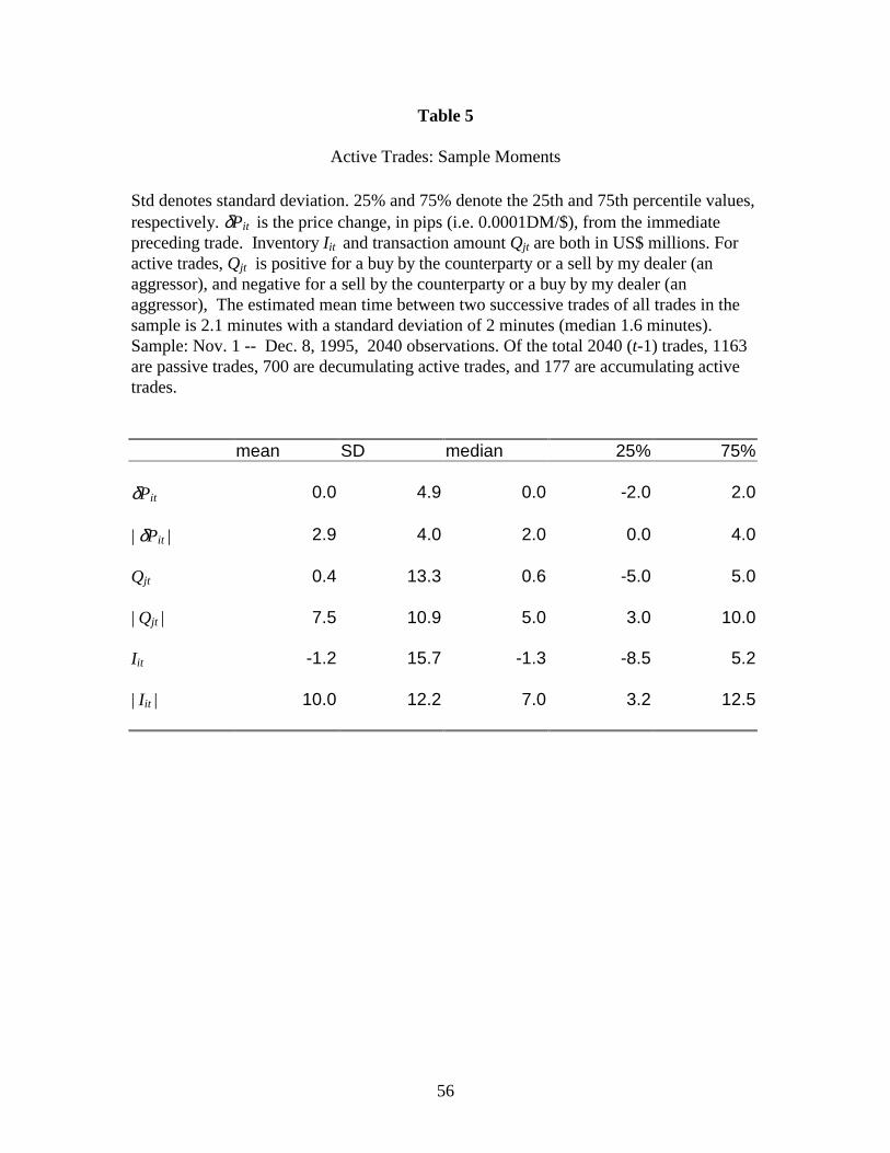
56
Table 5
Active Trades: Sample Moments
Std denotes standard deviation. 25% and 75% denote the 25th and 75th percentile values,respectively. δPit is the price change, in pips (i.e. 0.0001DM/$), from the immediatepreceding trade. Inventory Iit and transaction amount Qjt are both in US$ millions. Foractive trades, Qjt is positive for a buy by the counterparty or a sell by my dealer (anaggressor), and negative for a sell by the counterparty or a buy by my dealer (anaggressor), The estimated mean time between two successive trades of all trades in thesample is 2.1 minutes with a standard deviation of 2 minutes (median 1.6 minutes).Sample: Nov. 1 -- Dec. 8, 1995, 2040 observations. Of the total 2040 (t-1) trades, 1163are passive trades, 700 are decumulating active trades, and 177 are accumulating activetrades.
mean SD median 25% 75%
δPit 0.0 4.9 0.0 -2.0 2.0
| δPit | 2.9 4.0 2.0 0.0 4.0
Qjt 0.4 13.3 0.6 -5.0 5.0
| Qjt | 7.5 10.9 5.0 3.0 10.0
Iit -1.2 15.7 -1.3 -8.5 5.2
| Iit | 10.0 12.2 7.0 3.2 12.5
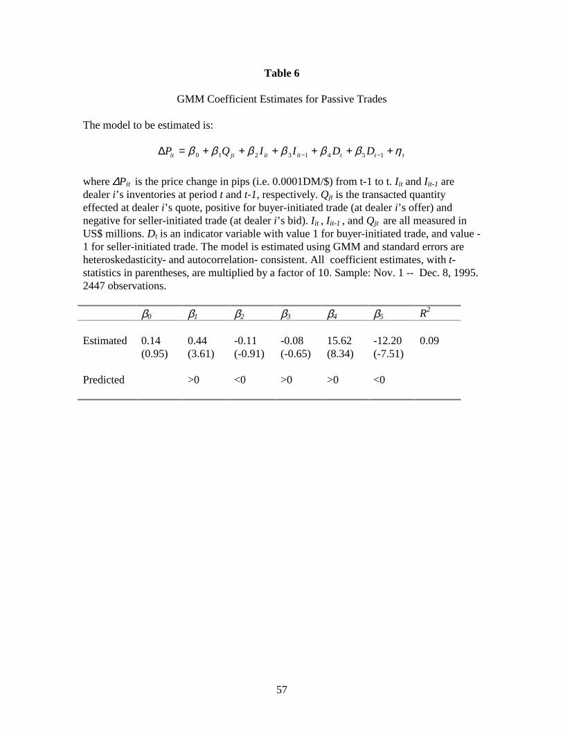
57
Table 6
GMM Coefficient Estimates for Passive Trades
The model to be estimated is:
∆P Q I I D Dit jt it it t t t= + + + + + +− −β β β β β β η0 1 2 3 1 4 5 1
where ∆Pit is the price change in pips (i.e. 0.0001DM/$) from t-1 to t. Iit and Iit-1 aredealer i’s inventories at period t and t-1, respectively. Qjt is the transacted quantityeffected at dealer i’s quote, positive for buyer-initiated trade (at dealer i’s offer) andnegative for seller-initiated trade (at dealer i’s bid). Iit , Iit-1 , and Qjt are all measured inUS$ millions. Dt is an indicator variable with value 1 for buyer-initiated trade, and value -1 for seller-initiated trade. The model is estimated using GMM and standard errors areheteroskedasticity- and autocorrelation- consistent. All coefficient estimates, with t-statistics in parentheses, are multiplied by a factor of 10. Sample: Nov. 1 -- Dec. 8, 1995.2447 observations.
β0 β1 β2 β3 β4 β5 R2
Estimated 0.14 0.44 -0.11 -0.08 15.62 -12.20 0.09(0.95) (3.61) (-0.91) (-0.65) (8.34) (-7.51)
Predicted >0 <0 >0 >0 <0

58
Table 7
Quote shading: Customer trades vs. dealer trades
The model to be estimated is:
∆P Q I I D Dit jt it it t t t= + + + + + +− −β β β β β β η0 1 2 3 1 4 5 1
The model is estimated for two subsets of passive trades, time-t customer trades only andtime-t dealers trades (Reuters direct and brokered) only. ∆Pit is the price changemeasured in pips (i.e. 0.0001DM/$) from t-1 to t. Iit and Iit-1 are dealer i’s inventories atperiod t and t-1, respectively. Qjt is the transacted quantity effected at dealer i’s quote,positive for buyer-initiated trade (at dealer i’s offer) and negative for seller-initiated trade(at dealer i’s bid). Iit , Iit-1 , and Qjt are all measured in US$ millions. Dt is an indicatorvariable with value 1 for buyer-initiated trade, and value -1 for seller-initiated trade. Themodel is estimated using GMM and standard errors are heteroskedasticity- andautocorrelation- consistent. All coefficient estimates, with t-statistics in parentheses, aremultiplied by a factor of 10. Sample: Nov. 1 -- Dec. 8, 1995.
(1) time-t customer trades only:(190 observations)
β0 β1 β2 β3 β4 β5 R2
Estimated -0.87 0.37 -0.47 0.16 15.53 -11.95 0.09(-1.40) (1.64) (-2.29) (0.60) (2.08) (-2.09)
Predicted >0 <0 >0 >0 <0
(2) time-t dealers trades (Reuters direct and brokered) only:(1291 observations)
β0 β1 β2 β3 β4 β5 R2
Estimated 0.38 0.34 0.15 -0.32 24.34 -10.84 0.15(1.94) (2.04) (0.79) (-1.64) (10.16) (-5.22)
Predicted >0 <0 >0 >0 <0

59
Table 8
GMM Coefficient Estimates for Active Trades
The model to be estimated is:
δη
P b b b I b I Ib T T b D b D D
it t t t t it t it t it t t
t t t t t t t t t t t
= + − − + + − −+ − − − − + + − − +
− − − − − − − −
− − − − − − −
01 1 02 1 1 1 1 1 2 1 1 1
3 1 1 1 4 1 1 5 1 1
1 11 1 1 1
Θ Ω Θ Ω Θ Ω Θ ΩΩ Θ Ω Θ Θ
( ( ) ) ( ( ) )( ( ) ( )( )) ( ( ))
where δPit is the price change, measured in pips (i.e. 0.0001DM/$), from the immediate preceding trades at t. Iit and Iit-1, in US$millions, are dealer i’s inventories at period t and t-1, respectively. Θt is an indicator variable with value of 1 for passive trades, andvalue of 0 for active trades. Ωt is an indicator variable with value of 1 for decumulating active trade, and value of 0 for accumulatingactive trade. Tt is also an indicator variable for accumulating active trade, with value of 1 when dealer i is long, and value of -1 whendealer i is short. (For definition of types of trades, please refer to the text.) Dt is an indicator variable with value 1 for dealer i’s sell,and value of -1 for dealer i’s buy. The model is estimated using GMM and standard errors are heteroskedasticity- and autocorrelation-consistent. All coefficient estimates, with t-statistics in parentheses, are multiplied by a factor of 10. Sample: Nov. 1 -- Dec. 8, 1995,2040 observations
b01 b02 b1 b2 b3 b4R b4
B b4C b5
R b5B R2
Estimated 0.72 -1.19 -0.20 0.05 5.67 -10.36 -16.49 -21.55 -14.29 -16.10 0.12(0.29) (-0.45) (-1.80) (0.67) (1.84) (-3.29) (-9.07) (-4.98) (-3.13) (-8.06)
Predicted >0 <0 >0 <0 <0 <0 <0 <0
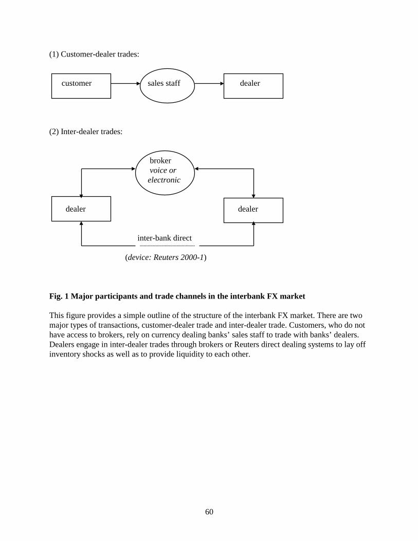
60
(1) Customer-dealer trades:
customer sales staff dealer
(2) Inter-dealer trades:
broker voice orelectronic
dealer dealer
inter-bank direct
(device: Reuters 2000-1)
Fig. 1 Major participants and trade channels in the interbank FX market
This figure provides a simple outline of the structure of the interbank FX market. There are twomajor types of transactions, customer-dealer trade and inter-dealer trade. Customers, who do nothave access to brokers, rely on currency dealing banks’ sales staff to trade with banks’ dealers.Dealers engage in inter-dealer trades through brokers or Reuters direct dealing systems to lay offinventory shocks as well as to provide liquidity to each other.

61
signal Wt receive observe signal hit observe signal hit observe signal yt quote Pit trade Qjt incre.dt yt+1 quote Pit+1 incre.dt+1 yt+ 2 quote Pit+2 incre.dt+2
Period: t (passive) t +1 (active) t +2 (active)
Fig. 2 Time indexing of trades and sequencing of events
This figure depicts the time/event sequence of the model. At time t = 1,2,..., T, it can be either apassive trade effected at dealer i’s quote, or an active trade which is initiated by dealer i and iseffected at other dealer’s quote. The figure depicts three trades: a passive trade at time t, followedby two active trades at t+1 and t+2. Public signal arrives in each time period; private signal Wt isonly present with a passive trade. Thus, information increment dt to FX fundamental valueincorporates revelation of both public and private information subsequent to a passive trade, butonly public information subsequent to an active trade.

62
Date 11/7 Currency: DM/$ DealerName
Value Date 11/9
CUSTOMER BUY SOLD RATE NET POSITION AVERAGE
($ mil.) ($ mil.) (DM/US$) ($ mil.) (DM/US$)Previousbalance
-22.6
BANK 1 B 5 1.4151 -17.6BANK 2 B 8 51 -9.6BANK 3 Q 2 50 -11.6COLLEAGUE 1 5 48 -6.6IMM 50 (6.25) 4.4 48 -11.0BANK 4 Q 3 47 -14.0 1.4151CUSTOMER 1 S 17.22 (24.375) 53BANK 5 Q 10 53BANK 6 B 5 54 -12.0BANK 7 ** R 10 50 -2.0... ... ... ... ... ... ...
Fig. 3. Example: one of my dealer’s actual trading blotters on November 7, 1995.
This figure provides an example of one of many trade blotters recorded by my DM/US$ dealerevery day. Each page starts with a balance from the previous page, or previous day if it is the firstblotter of a trading day. The first column is the counterparty identity of each trade, such as thename of a corporation in a customer trade, the name of a bank in an inter-dealer trade, or thename of the dealer’s colleague in an internal deal. The second column indicates the tradechannels, where B stands for voice broker (by name of the broker), Q for electronic broker, S forthe name of the salesperson involved in a customer trade, and R for Reuters direct trade. Anumber in the second column associated with an entry of “IMM” in the first column indicates thenumber of contracts traded on the IMM futures market. Entries in the “BUY” and “SELL”columns are in millions of U.S. dollars. When the original trade amount is in DMs, such as anIMM trade with contract size denominated in DMs or a trade involving a customer with a DMinvoice, my dealer enters the DM amount as well in parentheses, and then convert the DMamount to U.S. dollars at the corresponding DM/US$ trade price for position keeping.
** For this Reuters direct trade, I match up with Reuters 2000-1 records and identify the time as14:41 GMT, and the quoted spread 50-55. Since the dealer is buying at the bid, this trade isidentified as an incoming trade.

63
__________________________________________________________________________
From CODE BANK NAME * 1441GMT 071195 */4260Our terminal: CODE Our user: DEALER NAME
DM 10# 5055
I SELL# VAL 09NOV95# TO CONFIRM AT 1.4150 I BUY 10 MIO USD# MY USD TO USD DIRECT# THANKS AND BYE
VAL 09NOV95MY DEM TO BANK NAME FRANKFURTTO CONFIRM AT 1.4150 I SELL 10 MIO USD
## INTERRUPT #
# END REMOTE #
( 239 CHARS)__________________________________________________________________________
Fig 4. Example of an actual Reuters Dealing 2000-1 communication at 14:41 GreenwichMean Time (GMT) on November 7, 1995.
The example in this figure describes an incoming trade in which another dealer requests a quotefor $10 million worth of DMs from my dealer, and hit my dealer’s bid price of 1.4150 DM/US$(The offer side of the two-way quote is 1.4155 DM/US$). Such a $10 million trade is considerednormal among major DM/US$ dealers who maintain “$10 million relationship” with each other.Note that the bid-ask spread of 0.0005 DM/US$ (or 5 pips) is only 3.5 basis points of the tradesize. Coded information in the first two lines (in italics) indicates the identities of the two parties(actual names disguised) involved in this inter-dealer direct trade. The conversation is veryconcise, often in pre-programmed Reuters language, so that a trade can be completed in just afew seconds. The Reuters 2000-1 dealing system allows a FX dealer to conduct suchconversations with four dealers simultaneously.

64
1.37
1.38
1.39
1.4
1.41
1.42
1.43
1.44
1.45
1.4611
01
1101
1102
1103
1103
1106
1107
1108
1108
1109
1109
1110
1110
1113
1114
1114
1115
1115
1116
1116
1117
1120
1120
1121
1127
1127
1128
1128
1129
1129
1130
1130
1201
1204
1205
1206
1207
1207
1208
1208
date
DM
/$
Fig. 5 Transaction price: DM/$, Nov. 1 - Dec. 8, 1995.
The figure plots the transaction price of DM/$ of each incoming passive trade over the entire 25-day sample period. The sample period, Nov. 1 - Dec. 8, 1995, covers 25 continuous trading daysexcept for (1) weekends and (2) Thanksgiving Day (11/23) when the U.S. operation is closed,and the day before (11/22) and after (11/24) when the dealer, like most other North Americandealers, did not quote or trade in the Reuters 2000-1 direct interbank market. Passive tradesinclude customer trade, internal deal, limit order, Reuters incoming trade, and brokered tradewhich is signed by quote-based methodology and determined as incoming passive trades. Notethat the date (x-axis) tick mark is not evenly distributed, indicating different trade volume (interms of numbers of passive trades) across trading days.

65
-200
-150
-100
-50
0
50
100
150
200
1101
1101
1102
1103
1103
1106
1107
1108
1108
1109
1109
1110
1110
1113
1114
1114
1115
1115
1116
1116
1117
1120
1120
1121
1127
1127
1128
1128
1129
1129
1130
1130
1201
1204
1205
1206
1207
1207
1208
1208
date
inve
ntor
y in
$m
m
-200
-150
-100
-50
0
50
100
150
200
1101
1102
1103
1106
1107
1108
1109
1110
1113
1114
1115
1116
1117
1120
1121
1127
1128
1129
1130
1201
1204
1205
1206
1207
1208
date
clos
ing
posi
tion
in $
mm
Fig. 6 Net inventory and daily closing position in millions of US$, Nov. 1 - Dec. 8, 1995.
The chart at the top plots the $DM dealer’s net position in millions of US$ at the time of eachincoming passive trade over the entire 25-day sample period. Note that the date (x-axis) tickmark is not evenly distributed, indicating different trade volume (in terms of numbers of passivetrades) across trading days.
The chart at the bottom plots the dealer’s daily closing inventory in millions of US$ over the 25-day sample period. The chart has the same scale as the one at the top.

66
-100
-80
-60
-40
-20
0
20
40
1302
1520
1543
1548
1638
1651
1731
Greenwich Mean Time (GMT)
inve
ntor
y in
$m
m
1.394
1.396
1.398
1.4
1.402
1.404
1.406
1.408
DM
/$ p
rice
Fig. 7 Transaction price and inventory for all passive trades on Nov. 17, 1995.
The figure depicts both transaction price and inventory for all incoming passive trades on Nov.17, 1995, the day with median turnover in the sample of 25 trading days, Nov. 1 - Dec. 8, 1995.Passive trades include customer trade, internal deal, limit order, Reuters incoming trade, andbrokered trade which is signed by quote-based methodology and determined as incoming passivetrade.

67
0
1
2
3
4
5
6
7
8
9
10
1 2 3 4 5 6 7 8 9 10 11 12 13 14 15 16 17 18 19 20 21 22 23 24 25 26 27 28 29 30incoming passive trade
pips
(1pi
p =
0.00
01D
M/$
)
$100mm buy
$50mm buy
$20mm buy
$10mm buy
Fig. 8 Price response process following an initial $US buy order against DM.
The figure depicts the price response process according to a VAR (8) system of price, inventoryand passive trade, subsequent to initial $US buy orders of the indicated sizes.

68
0
0.1
0.2
0.3
0.4
0.5
0.6
0.7
0.8
1 2 3 4 5 6 7 8 9 10 11 12 13 14 15 16 17 18 19 20 21 22 23 24 25 26 27 28 29 30
incoming passive trade
shor
t inv
ento
ry p
ositi
on a
s a
frac
tion
of in
itial
buy
The four curves (from top to bottom, respectively) correspond to initial $US buy orders of
$10mm, $20mm, $50mm and $100mm.
Fig. 9 Inventory adjustment process following an initial $US buy order against DM.
The figure depicts the inventory adjustment process according to a VAR(8) system of price,inventory and passive trade, subsequent to initial $US buy orders of the indicated sizes.Immediately following a initial $US buy, the dealer has a short position in $US amounting toonly about 72.4% of the size of initial buy order because of anticipatory inventory build-up inadvance.

69
-2
0
2
4
6
8
10
12
14
1 2 3 4 5 6 7 8 9 10 11 12 13 14 15 16 17 18 19 20 21 22 23 24 25 26 27 28 29 30
incoming passive trade
perc
enta
ge o
f ini
tial b
uy q
uant
ity (%
$10mm buy
$20mm buy
$50mm buy
$100mm buy
Fig. 10 Cumulative incoming passive sells following an initial $US buy order against DM.
The figure depicts the cumulative passive sells according to a VAR(8) system of price, inventoryand passive trade, throughout 30 incoming passive trades subsequent to initial $US buy orders ofthe indicated sizes. Such incoming sells allow the dealer to cover part of his short $US position,whose size immediately following the initial buy order is equal to about 72.4% of the initial buyorder.