Consumption-Based Asset Pricing with a Reference …ftp.zew.de/pub/zew-docs/dp/dp0632.pdf · Consumption-Based Asset Pricing with a Reference Level: New Evidence from the ... According

Discussion Paper No. 06-032

Consumption-Based Asset Pricing

with a Reference Level:

New Evidence from the Cross-Section

of Stock Returns

Joachim Grammig and Andreas Schrimpf

Discussion Paper No. 06-032

Consumption-Based Asset Pricing

with a Reference Level:

New Evidence from the Cross-Section

of Stock Returns

Joachim Grammig and Andreas Schrimpf

Die Discussion Papers dienen einer möglichst schnellen Verbreitung von neueren Forschungsarbeiten des ZEW. Die Beiträge liegen in alleiniger Verantwortung

der Autoren und stellen nicht notwendigerweise die Meinung des ZEW dar.

Discussion Papers are intended to make results of ZEW research promptly available to other economists in order to encourage discussion and suggestions for revisions. The authors are solely

responsible for the contents which do not necessarily represent the opinion of the ZEW.

Download this ZEW Discussion Paper from our ftp server:

ftp://ftp.zew.de/pub/zew-docs/dp/dp06032.pdf

Non-technical Summary

According to classical asset pricing theory, differences in expected returns across

assets must be ultimately accounted for by differences in the covariation of the

asset’s return with consumption growth. Despite its theoretical purity, however,

the canonical consumption-based asset pricing model (CCAPM) has had a disap-

pointing performance in past empirical tests.

In this paper, we formally estimate several extended versions of the model on

common U.S. stock market data. In particular, we focus on the extension of the

standard preferences by a reference level of consumption and investigate the empir-

ical performance of this new approach in explaining the cross-sectional variation of

average stock returns compared to well-established benchmark models. Several ver-

sions of a consumption-based model with a benchmark level of consumption have

recently been proposed and estimated by Garcia, Renault and Semenov (2003).

Their focus, however, was to test the conditional moment restrictions using the

market portfolio and the Treasury-Bill as test assets. We extend their analysis by

testing the unconditional moment restrictions of several of their proposed models

on a broad cross-section of test assets, namely Fama and French’s 25 portfolios

sorted according to size and book-to-market.

Apart from employing this challenging set of test assets, this paper also motivates a

specification of the reference level model which takes the return on human capital

into account. Garcia et al. (2003) consider a specification, where the reference

level is modelled as a function of the contemporaneous return of a market portfolio

proxy. As emphasized by Roll (1977), a value-weighted stock market portfolio may

not be an adequate proxy for the portfolio of total wealth since the human capital

component of aggregate wealth is neglected. In this paper, we therefore consider

an extended model in which the reference level does not only depend on the return

of asset income, but also on the return of human capital. Following Jagannathan

and Wang (1996), Lettau and Ludvigson (2001b) and Dittmar (2002) we use labor

income growth as a proxy for the return on human capital.

We present empirical evidence that the model extensions by a reference level have

the potential to improve the empirical performance of the consumption-based asset

i

pricing framework. The pricing errors of several of the new reference level models

are considerably smaller than those of the original specification of the CCAPM.

Furthermore, we find that the model augmented by human capital does a good job

in explaining the cross-sectional variation in average returns across the 25 Fama-

French portfolios with pricing errors close to those of the scaled factor model by

Lettau and Ludvigson (2001b).

ii

Consumption-Based Asset Pricing with aReference Level: New Evidence from the

Cross-Section of Stock Returns

Joachim Grammig and Andreas Schrimpf∗

May 16, 2006

Abstract

This paper presents an empirical evaluation of recently proposed asset pricingmodels which extend the standard preference specification by a reference level ofconsumption. The novelty is that we use a broad cross-section of test assets, whichprovides a level playing field for a comparison to well-established benchmark models.We also motivate a specification that accounts for the return on human capital asa determinant of the reference level. We find that this extension does a good jobin explaining the cross-sectional variation in average returns across the 25 Fama-French portfolios with pricing errors close to those of Lettau/Ludvigson’s celebratedscaled factor models.

JEL Classification: G12Keywords: Consumption-based Asset Pricing, Cross-Section of Stock Returns, Reference Level

∗Contact details authors. Joachim Grammig, University of Tubingen, Department of Eco-nomics, Mohlstr. 36. 72074 Tubingen, Germany, email: [email protected],phone: +49 7071 2976009, fax: +49 7071 295546; Andreas Schrimpf, Centre for EuropeanEconomic Research (ZEW), Mannheim, P.O. Box 10 34 43, 68034 Mannheim, Germany, email:[email protected], phone: +49 621 1235160, fax: +49 621 1235223. Joachim Grammig is alsoresearch fellow at the Centre for Financial Research (CFR), Cologne. We thank participants atthe 2006 annual meeting of the econometrics committee (Ausschuss fur Okonometrie) of the Ger-man Economic Association, the 2006 meetings of the Midwest Finance Association (Chicago) andEastern Finance Association (Philadelphia) for helpful discussions. We thank Kenneth Frenchand Sydney Ludvigson for providing their data on their webpages. We are also grateful to AndreiSemenov and Erik Luders for helpful comments and Stefan Frey for providing us with a librarywith GAUSS procedures for GMM estimation.

1 Introduction

Despite its theoretical appeal, the consumption-based asset pricing model (CCAPM)

has as yet achieved little empirical success in calibration exercises or formal econo-

metric testing [See e.g. Mehra and Prescott (1985), Hansen and Singleton (1982),

Cochrane (1996) or Lettau and Ludvigson (2001b) etc.]. The empirical failure of

the model has sparked a wave of research over the past 20 years aimed at improv-

ing the canonical CCAPM and making the model consistent with the empirical

facts.1

This paper presents an empirical evaluation of recently proposed asset pricing

models which extend the standard preferences by a reference level of consumption.

The novelty of our paper is that we use a broad cross-section of test assets in

order to evaluate the new models. So far, the conditional implications of asset

pricing models with a reference level have been tested using a market portfolio

proxy and the Treasury-Bill as basic test assets. In our empirical investigation

we use Fama and French’s 25 portfolios sorted by size and book-to-market, which

provides a level playing field for a comparison of the new models to well-established

benchmark models. We also motivate a specification that accounts for the return

on human capital as a determinant of the reference level. This augmented model

delivers a quite encouraging empirical performance with pricing errors which are

close to those of the celebrated scaled CCAPM by Lettau and Ludvigson (2001b).

According to Cochrane (1997), the recently proposed theoretical modifications to

the standard consumption-based framework can be primarily classified into two

lines of research. One class of models tackles the empirical shortcomings of the

standard CCAPM by abandoning the assumption of perfect capital markets. Mod-

els of this class focus on incomplete markets, survivorship bias, market imperfec-

tions, limited stock market participation on behalf of the population or are based

on behavioral explanations. The second line of research maintains the framework

of a representative investor and perfect capital markets but concentrates on mod-

1An overview and a critical reflection of recent approaches to solve the so-called ”equitypremium puzzle” is provided e.g. in Mehra and Prescott (2001) or Mehra (2003). An excellentrecent survey on the topic is provided by Cochrane (2006).

1

ifications of investor preferences. Examples for modified preferences include for

instance the model by Epstein and Zin (1991) which disentangles risk aversion and

intertemporal substitution and the literature on habit formation [e.g. Abel (1990),

Constantinides (1990), Ferson and Constantinides (1991), Campbell and Cochrane

(1999), Campbell and Cochrane (2000)]. As pointed out by Chen and Ludvigson

(2003), “habit-formation” constitutes a leading approach within this class of mod-

els. The central idea is that individuals get accustomed to a certain standard of

living. They do not derive utility from consumption taken by itself as in the tradi-

tional economic models. Instead, the well-being of the individual depends on how

much she consumes relative to a certain benchmark level.

Within the class of habit models, one can further distinguish between internal and

external habit formation. Internal habit formation implies that the benchmark

level is influenced by the investor’s own consumption and saving decisions. By

contrast, in models with external habit formation habit is not affected by the

investor’s decisions but depends on past aggregate consumption and can thus be

interpreted as the benchmark level for the society as a whole. External habit

formation expresses the idea that people want to maintain their relative standing

in society often referred to as “Catching up with the Joneses” behavior, as noted

in Abel (1990). The models considered in this paper are based on the concept

of external habit formation. When habit is a function not only of past aggregate

consumption but also current consumption, this leads to the more general“Keeping

up with the Joneses” specification. This is true for instance in the model by

Campbell and Cochrane (1999), where also contemporaneous consumption enters

the habit function along with past consumption levels. An important feature of

this model is counter-cyclical variation of risk-aversion that depends on the state

of the economy. In a recession – a situation in which consumption has fallen close

to the benchmark level – investors’ level of risk aversion rises. In this way, the

model offers interesting insights regarding the interplay of financial markets and

the state of the economy.

The class of consumption-based asset pricing models with a reference level which

2

we investigate in this paper has been proposed by Garcia et al. (2003). The

main focus of their empirical investigation with U.S. monthly data was to test the

conditional moment restrictions using a market portfolio proxy and the Treasury-

Bill as test assets. We extend their analysis by estimating and testing several

of their proposed models on a broad cross-section of test assets. We use Fama

and French’s 25 portfolios sorted according to size and book-to-market as our

test assets.2 Apart from employing this challenging set of test assets, this paper

also proposes an extended version of the model originally proposed by Garcia

et al. (2003). When specifying their reference level as a function of both past

and current variables, the authors model their reference level also as a function of

the contemporaneous return of a market portfolio proxy. As pointed out by Roll

(1977), a value-weighted stock market portfolio may not be an adequate proxy for

the total wealth portfolio since the human capital component of aggregate wealth is

neglected. Dittmar (2002) has argued that integrating a measure of human capital

into a non-linear stochastic discount factor is essential for pricing the cross-section

of stock returns. Dittmar remains agnostic about the specific form of the utility

function and approximates the SDF using a Taylor expansion. The SDF proxy he

obtains is a polynomial in the return of aggregate wealth. An important factor

of the empirical success of his model is to consider the return on human capital

in the specification of the return on aggregate wealth. Drawing on that work, we

therefore consider an extended model in which the reference level does not only

depend on the returns of asset income, but also on the returns of human capital.

As in Jagannathan and Wang (1996), Lettau and Ludvigson (2001b) and Dittmar

(2002), we use labor income growth as a proxy for the return on human capital.

Another novelty of this paper is a performance comparison of the new models to

well-established empirical asset pricing models. One of the most successful models

in explaining the cross-section of stock returns is arguably the three-factor model

by Fama and French (1993). Owing to its empirical success in explaining the cross-

section of returns and its widespread use, it serves as a natural benchmark model.

2In order to check the robustness of our results we also estimated the models using ten sizeportfolios, which were employed in Cochrane (1996). The results are qualitatively similar andlead to the same conclusions.

3

An important contribution has been the work by Lettau and Ludvigson (2001a,

2001b) who investigate a conditional linearized version of the CCAPM. Specifically,

Lettau and Ludvigson use the log consumption-wealth ratio (cay) as a conditioning

variable, an instrument which has good forecasting properties for stock returns.

Since Lettau Ludvigson’s scaled CCAPM does a particularly good job in pricing

the 25 Fama-French portfolios and is also solely based on macroeconomic factors it

serves as an important benchmark for asset pricing models with a reference level.

Our paper is rooted in the empirical literature on representative agent models,

which are estimated using aggregate consumption data, as pioneered by Hansen

and Singleton (1982). Whereas earlier papers looked mainly at statistical rejections

and only considered a few test assets, the recent focus has shifted to looking at

economic pricing errors directly (RMSE, pricing error plots) and testing the mod-

els on the cross-section of size and book-to-market portfolios (Cochrane 2006).

Most recently, there has been a renewed interest in empirical investigations of

the consumption-based asset pricing approach in this contemporaneous empirical

setting. Related work includes for instance Yogo (2006), who focuses on the con-

sumption of durables, or Piazzesi, Schneider and Tuzel (2006), who analyze the

influence of the share of housing consumption in total consumption. Ait-Sahalia,

Parker and Yogo (2004) motivate a utility specification where households consume

both basic and luxury goods. They are able to show that a linearized CCAPM

based on luxury consumption data performs considerably better in explaining the

cross-section of returns than the conventional specification based on aggregate

consumption data. Parker and Julliard (2005) examine the long-run properties of

the consumption-based model and also test their model using the 25 Fama-French

portfolios.

The main results of this paper can be summarized as follows. Asset pricing models

which account for a reference level of consumption can considerably improve the

empirical performance of the standard CCAPM. However, our results show that

it is important to account for the growth of human capital in the specification for

the reference level. The performance of models with alternative specifications for

4

the reference level is not that satisfactory. However, the human capital extended

model delivers quite encouraging results, with pricing errors of the model close to

those of Lettau-Ludvigson’s scaled CCAPM and more sensible parameter estimates

from an economic point of view. Enlarging the sample period, and using more

recent data comprising the internet boom, the human capital extended model even

outperforms this celebrated benchmark model and delivers pricing errors close to

the theoretically much less appealing Fama-French three-factor model.

The remainder of the paper is organized as follows. In section 2 we present the

data. We then lay out the theoretical framework with a brief discussion of the

newly proposed consumption-based asset pricing models with a reference level.

Section 4 presents estimation and test results for the new models and compares

their empirical performance to benchmark asset pricing models. Section 5 con-

cludes.

2 A Level Playground

This section describes the data used in our empirical analysis. By merging data

sets which have already been used in a number of empirical studies [e.g. Fama

and French (1993), Lettau and Ludvigson (2001b) etc.] we want to establish a

level playing field on which the different models can show their relative merits

and model performances can be compared. The base sample period is 1963:Q1-

1998:Q3, the same as in Lettau and Ludvigson (2001b). As outlined above, Lettau

and Ludvigson’s scaled CCAPM provides a natural benchmark, so we chose the

same sample period for the sake of comparability. We also report estimation results

for the whole sample on which we have data available and which overlaps the

“internet boom”, 1952:Q2-2002:Q1.

Our test assets are Fama and French’s 25 portfolios sorted by size and book-to-

market characteristics.3 Nominal data are converted into ex-post real returns by

3These data are regularly updated and provided by Kenneth French on his webpage(http://mba.tuck.dartmouth.edu/pages/faculty/ken.french/data_library.html).

5

dividing nominal gross returns by the corresponding gross inflation rate. The

inflation rate was calculated from the seasonally adjusted Consumer Price Index

(CPI) for all urban consumers.4 Since the data from Kenneth French’s webpage

are only available at a monthly frequency, the data were converted into quarterly

data in order to match the frequency of the consumption data.

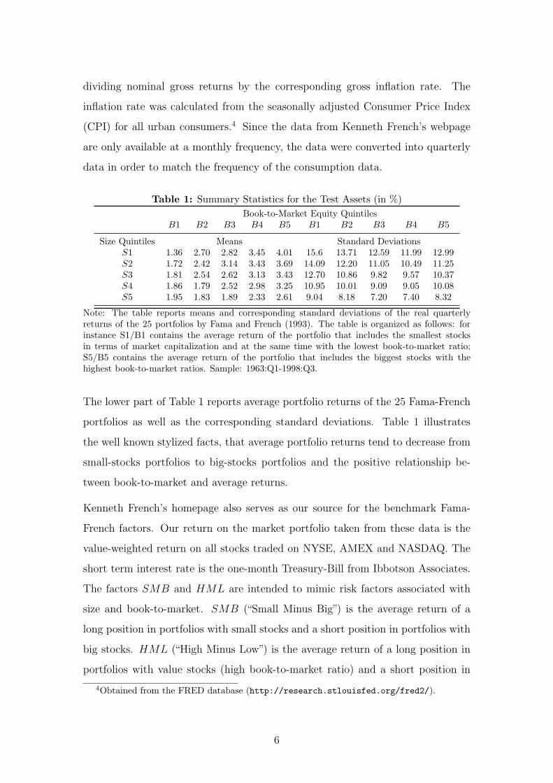
Table 1: Summary Statistics for the Test Assets (in %)Book-to-Market Equity Quintiles

B1 B2 B3 B4 B5 B1 B2 B3 B4 B5

Size Quintiles Means Standard DeviationsS1 1.36 2.70 2.82 3.45 4.01 15.6 13.71 12.59 11.99 12.99S2 1.72 2.42 3.14 3.43 3.69 14.09 12.20 11.05 10.49 11.25S3 1.81 2.54 2.62 3.13 3.43 12.70 10.86 9.82 9.57 10.37S4 1.86 1.79 2.52 2.98 3.25 10.95 10.01 9.09 9.05 10.08S5 1.95 1.83 1.89 2.33 2.61 9.04 8.18 7.20 7.40 8.32

Note: The table reports means and corresponding standard deviations of the real quarterlyreturns of the 25 portfolios by Fama and French (1993). The table is organized as follows: forinstance S1/B1 contains the average return of the portfolio that includes the smallest stocksin terms of market capitalization and at the same time with the lowest book-to-market ratio;S5/B5 contains the average return of the portfolio that includes the biggest stocks with thehighest book-to-market ratios. Sample: 1963:Q1-1998:Q3.

The lower part of Table 1 reports average portfolio returns of the 25 Fama-French

portfolios as well as the corresponding standard deviations. Table 1 illustrates

the well known stylized facts, that average portfolio returns tend to decrease from

small-stocks portfolios to big-stocks portfolios and the positive relationship be-

tween book-to-market and average returns.

Kenneth French’s homepage also serves as our source for the benchmark Fama-

French factors. Our return on the market portfolio taken from these data is the

value-weighted return on all stocks traded on NYSE, AMEX and NASDAQ. The

short term interest rate is the one-month Treasury-Bill from Ibbotson Associates.

The factors SMB and HML are intended to mimic risk factors associated with

size and book-to-market. SMB (“Small Minus Big”) is the average return of a

long position in portfolios with small stocks and a short position in portfolios with

big stocks. HML (“High Minus Low”) is the average return of a long position in

portfolios with value stocks (high book-to-market ratio) and a short position in

4Obtained from the FRED database (http://research.stlouisfed.org/fred2/).

6

portfolios with growth stocks (low book-to-market ratio). For further details on

the construction of SMB and HML see Fama and French (1993). All nominal

data were converted into real returns as described above. In order to match the

frequency of the consumption data, monthly returns had to be transformed into

quarterly returns.

The consumption data (real and per capita) used in this empirical study were ob-

tained from Sydney Ludvigson’s website. These data are defined as consumption

of nondurables and services excluding shoes and clothing. Time series of the con-

ditioning variable cay and labor income (real, per capita) were also obtained from

Sydney Ludvigson’s website.5 The time series of labor income was used for cal-

culating the growth rate of labor income needed for the estimation of our human

capital augmented reference level model.

3 Consumption-Based Asset Pricing with a Ref-

erence Level

In this section we review the theoretical framework of the consumption-based asset

pricing models with a reference level introduced by Garcia et al. (2003). First, a

few fundamental concepts are discussed. Then we turn to the modeling strategy

for the reference level and discuss how the specification for the reference level can

be augmented by human capital.

3.1 Basic concepts

Consumption-based asset pricing models with a reference level are best written in

their stochastic discount factor representation. When the law of one price holds,

there exists a stochastic discount factor (SDF) Mt+1 that prices returns:

5http://www.econ.nyu.edu/user/ludvigsons/. The cay variable is obtained as the residualfrom the cointegrating relationship between consumption, asset income and labor income. SeeLettau and Ludvigson (2001b, 2001a) for more information on data construction and on thetheoretical motivation of the cay variable.

7

E[Mt+1Rit+1|Φt] = 1. (1)

Rit+1 denotes the gross-return of asset i (i = 1, . . . , N) and Φt represents the infor-

mation set of the investor available as of t. The basic setting for asset pricing mod-

els with a reference level builds on classic consumption-based asset pricing where

Equation (1) results from the first order conditions of an intertemporal consump-

tion allocation problem with time-separable utility. The stochastic discount factor

can then be interpreted as the marginal rate of substitution, Mt+1 = δU ′(Ct+1)U ′(Ct)

,

where δ denotes the subjective discount factor and U(·) is the period utility func-

tion. Assuming a power utility specification U(Ct) =C1−γ

t

1−γwith γ as the relative

risk aversion (RRA) parameter the SDF is then given by

Mt+1 = δ

(Ct+1

Ct

)−γ

. (2)

Asset pricing models with a reference level retain this basic framework, but with a

differently motivated period utility function U(·). Specifically, Garcia et al. (2003)

advocate an approach in which utility does not only depend on consumption Ct,

but also on consumption relative to a reference level Xt. Furthermore, the reference

level Xt also enters the utility function in its absolute level,6

U(Ct/Xt, Xt) =

(Ct

Xt

)1−γ

X1−ψt

sign(1− γ)sign(1− ψ), (3)

where sign(z) = 1 if z ≥ 0 and sign(z) = −1 if z < 0, which ensures that utility is

defined for all parameter values of interest. The parameter ψ controls the curvature

of utility over the benchmark level. Several alternative specifications are nested

as special cases. For instance with ψ = γ, Equation (3) reduces to the power-

utility CCAPM. With ψ = 1, the reference level itself does not enter the utility

function directly, and investor utility depends solely on consumption relative to her

6Campbell and Cochrane (1999) have pursued a different approach by assuming that thedifference between consumption and reference level enters the utility function.

8

benchmark. The reference level is assumed to be related to aggregate consumption

by identity in conditional expectations, i.e.

Et(Xt+τ ) = Et(Ct+τ ) ∀ τ ≥ 0. (4)

Throughout this paper the reference level is considered as external by the investor.

This implies that the reference level is a societal standard which the investor

conceives as the benchmark for her consumption decision. Therefore, the stochastic

discount factor which can be derived from Equation (3) takes the following form

Mt+1 = δ

(Ct+1

Ct

)−γ (Xt+1

Xt

)γ−ψ

. (5)

3.2 Modeling the Reference Level

To provide an empirically testable model, further assumptions regarding the evo-

lution of the reference level Xt are necessary. Depending on the information set

available to the investor, Garcia et al. (2003) distinguish between two possible mod-

eling strategies. A first modeling strategy could assume that the investor only has

information up to period t when forming her benchmark level t+1. Specifically, it

is assumed that the reference level in t+1 equals the conditional expectation of the

future consumption level, where the investor’s information set in t only includes

past realizations of consumption levels, i.e. Xt+1 = E(Ct+1|Ct, Ct−1, . . .). This is

consistent with (4) for horizon τ = 1. In contrast to earlier papers which assumed

that habit only depended on consumption lagged by one period [e.g. (Abel 1990)],

Garcia et al. (2003) consider that reference levels react slowly to consumption. As-

suming adaptive expectations, a change in the reference level is a function of the

error when forming the reference level in the previous period, ∆Xt+1 = ρ(Ct−Xt).

Allowing for a constant a and iterating forward on Xt+1 = a+ ρCt +(1− ρ)Xt, we

obtain

9

Xt+1 =a

ρ+ ρ

∞∑i=0

(1− ρ)iCt−i. (6)

In this specification, which we refer to as “pure habit formation”, the habit level

thus depends on past realizations of consumption with declining weights.

In a second modeling strategy Garcia et al. (2003) assume that the investor uses

some information available in t + 1 when forming the reference level Xt+1. Specif-

ically, they argue that the contemporaneous log-return of the market portfolio,

rmt+1, qualifies as an important variable affecting the reference level.7 This paper

draws on this idea and extends it by arguing that the returns to human capital

should be taken into account, too. This argument is backed by classic and recent

literature. As emphasized for instance by Jagannathan and Wang (1996), aggre-

gate wealth also contains a human capital component. The same argument has

been put forth by Lettau and Ludvigson (2001b), who also estimate a “scaled hu-

man capital CAPM” (HCAPM) in their paper. Dittmar (2002) has argued for the

importance of incorporating a measure of human capital into pricing kernels. Ac-

cordingly, we assume that the growth rate of the log reference level is determined

by past log consumption growth, the log return on the market portfolio as well as

the log return on human capital rhct+1:

∆xt+1 = a0 +n∑

i=1

ai ·∆ct+1−i + b · rmt+1 + c · rhc

t+1. (7)

We refer to this specification as the “human capital (HC) extended model”. The

economic intuition behind this specification is the following: when wealth increases

in the economy (return on the market portfolio or the return on human capital

move up), the investor adjusts her benchmark to a higher level. Garcia et al.

(2003) assume that consumption growth equals the growth rate of the reference

level plus noise. Hence, combining (7) and (4) at horizon one, one can write

7Throughout this paper we use lower case letters to denote natural logs of the respectivevariable.

10

∆ct+1 = a0 +n∑

i=1

ai ·∆ct+1−i + b · rmt+1 + c · rhc

t+1 + εt+1. (8)

where εt+1 is an orthogonal innovation, Et[εt+1] = 0, Et[εt+1rmt+1] = 0 and Et[εt+1r

hct+1] =

0. Reference level growth can then be written as

Xt+1

Xt

= A

n∏i=1

[Ct+1−i

Ct−i

]ai (Rm

t+1

)b (Rhc

t+1

)c, (9)

where A = exp(a0). Plugging Equation (9) into (5), it follows that the SDF of the

HC-extended model is given by

Mt+1 = δAγ−ψ

[Ct+1

Ct

]−γ n∏i=1

[Ct+1−i

Ct−i

]ai(γ−ψ) (Rm

t+1

)b(γ−ψ) (Rhc

t+1

)c(γ−ψ). (10)

Following Garcia et al. (2003), we define δ∗ = δAγ−ψ and κ = b(γ − ψ). Equation

(10) can be rewritten as

Mt+1 = δ∗[Ct+1

Ct

]−γ n∏i=1

[Ct+1−i

Ct−i

]ai(γ−ψ) (Rm

t+1

)κ (Rhc

t+1

)κcb . (11)

Garcia et al. (2003) show that the elasticity of intertemporal substitution implied

by Equation (11) is given by σ = 1+b(γ−ψ)γ

= 1+κγ

.8 Hence, testing whether κ

equals zero means testing whether the elasticity of intertemporal substitution is

the inverse of the coefficient of relative risk aversion. This is one of the restrictive

assumptions in the standard CCAPM with power-utility.

The SDF representation in Equation (11) is a general specification that nests

various models proposed in the asset pricing literature as special cases. We turn to

the estimation of these models in the next section where we also address additional

assumptions for the empirical model as well as econometric issues.

8See Garcia et al. (2003) for further details on this result. They also show that a separationbetween risk aversion and intertemporal substitution is only possible when the reference leveldoes not only depend on past but also on contemporaneous variables.

11

4 Results and Discussion

In this section we discuss the estimation results for consumption-based asset pric-

ing models extended by a reference level. For the purpose of empirical performance

comparisons we round up the usual suspects. Along with the inevitable CAPM, the

CCAPM with power-utility serves as the natural benchmark, but we also present

the results for empirically more successful models. The competitors include Lettau-

Ludvigson´s scaled CCAPM and scaled CAPM, as well as the Fama-French three

factor model which – on its own playing field (size and book-to-market sorted

portfolios) – arguably represents the toughest challenge. Details about the re-

spective stochastic discount factor specifications and empirical methodologies are

delivered before discussing the respective empirical results. We report both first-

and two-stage GMM estimation results. First-stage GMM, though less efficient,

is preferable for model comparisons since the average pricing errors for the test

assets are weighted identically across all compared models. We do not make use

of instruments (managed portfolios). Instead we condition down and utilize the

unconditional implications of the basic pricing equation (1) for GMM estimation

of the parameters. Our basic test assets are the gross returns of the 25 Fama-

French portfolios sorted by size and book-to-market. The estimation results for

the sample period 1963:Q1-1998:Q3 used by Lettau and Ludvigson (2001) are re-

ported in tables 2 through 7. In our discussion of the economic interpretation of

the parameter estimates we focus on this sample period. The estimation results for

the extended sample period (1952:Q2-2002:Q1) can be found in tables B.1 to B.6

of the appendix. Following recommended practice we assess the empirical model

performances by average pricing error comparisons (Cochrane 2006). Figures 1

(sample period 1963:Q1-1998:Q3) and 2 (sample period 1952:Q2-2002:Q1) depict

pricing error plots and report root mean squared average pricing errors for models

of special interest. Additional pricing error plots can be found in figure 3 and in

figure C.1 of the appendix.

12

CCAPM with power-utility Asset pricing with a reference level was moti-

vated by the empirical weakness of the power utility CCAPM. Hence, this model

serves as the natural benchmark for our comparisons. Estimation results for the

model are reported in Table 2. We obtain the disturbing, yet familiar results.

The GMM estimate of the RRA parameter γ is large, but also quite imprecise,

and the estimate of the subjective discount factor is greater than one. The model

is furthermore rejected by Hansen’s (1982) JT -test.9 Figure 1 and 2 show that

the model fails to account for the cross-sectional return variation of the 25 Fama-

French portfolios. Overall, these results provide non-surprising further evidence

for the apparent dismal empirical performance of the CCAPM with power utility.

Table 2: CCAPM: estimation resultsFirst-Stage GMM Two-stage GMM

Estimate t-Statistic Estimate t-Statistic

δ 1.18 2.68 1.07 5.17γ 39.96 0.46 17.15 0.44

JT -Statistic 65.3 63.5p-value 0.0 0.0

Note: The estimation was carried out using gross returns of the testassets. Sample: 1963:Q1-1998:Q3.

Pure Habit Formation Garcia et al. (2003) propose an asset pricing model

in which the reference level is solely determined by past aggregate consumption

levels (“pure habit formation”). Equation (5) implies that for the calculation of

the model’s SDF one needs habit growth data, {Xt+1/Xt}. These data are not

directly observable. Garcia et al. (2003) suggest the following strategy to resolve

this problem. Assuming that the reference level evolves according to the adaptive

expectations hypothesis, habit can be expressed as a function of past consumption

levels with declining weights over time. Furthermore, assuming that the reference

level in t + 1 is equal to the conditional expected consumption in t + 1 one can

9It is well known that the JT -test may be unreliable in that the large sample distribution ofthe test statistic under the null is not well approximated in small samples. Among others Halland Horowitz (1996) and Altonji and Segal (1996) have pointed out that the JT -test frequentlyover-rejects in small samples. Given the rejection of the overidentifying restrictions of all modelsconsidered in this paper, including the Fama-French three factor model itself (see tables 7 andB.6) we do not focus on the interpretation of the test of overidentifying restrictions.

13

0 0.5 1 1.5 2 2.5 3 3.5 40

0.5

1

1.5

2

2.5

3

3.5

4

11 1213 14 15

21 22 23 2425

31 3233 34 354142 43 44455152

5354

55

Consumption−based Model: 1963Q1−1998Q3

Fitt

ed m

ean

retu

rns

(in %

)

Realized mean returns (in %)0 0.5 1 1.5 2 2.5 3 3.5 4

0

0.5

1

1.5

2

2.5

3

3.5

4

111213 14 15

2122 23 24 25

3132

33 34 354142 43 44 45515253 54 55

CAPM: 1963Q1−1998Q3

Fitt

ed m

ean

retu

rns

(in %

)

Realized mean returns (in %)

0 0.5 1 1.5 2 2.5 3 3.5 40

0.5

1

1.5

2

2.5

3

3.5

4

11

121314 15

2122

23 2425

31

3233 34 35

4142 43

4445

5152

53

54

55

Garcia−Renault−Semenov Model: 1963Q1−1998Q3

Fitt

ed m

ean

retu

rns

(in %

)


0

0.5

1

1.5

2

2.5

3

3.5

4

11

1213

1415

21

22

23 24

25

31 32

3334

35

41

4243

44

45

51

52

53

54

55

Human Capital extended Model: 1963Q1−1998Q3

Fitt

ed m

ean

retu

rns

(in %

)


0 0.5 1 1.5 2 2.5 3 3.5 40

0.5

1

1.5

2

2.5

3

3.5

4

11

12

13 14

15

21

22 23

2425

31

32

33

34

35

41

42

43 44

45

51

5253

54

55

Scaled CCAPM: 1963Q1−1998Q3

Fitt

ed m

ean

retu

rns

(in %

)


0

0.5

1

1.5

2

2.5

3

3.5

4

11

1213

14

15

21

22

23

24

25

31

32

33

34

35

41

42

43

44

45

51

52

53

54

55

Fama−French Model: 1963Q1−1998Q3

Fitt

ed m

ean

retu

rns

(in %

)


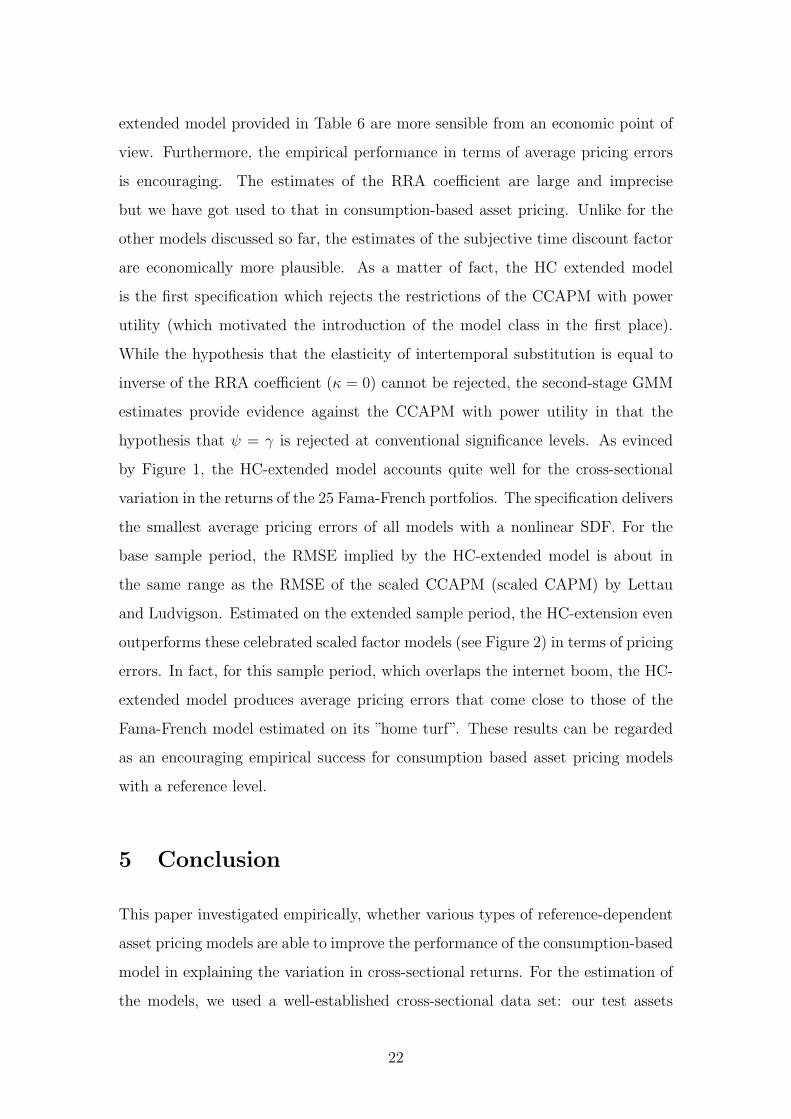
Figure 1: Consumption-based Asset Pricing Models and Benchmark Linear FactorModels: Fitted vs. Actual Mean Returns (in % per quarter). Sample period:

1963:Q1-1998:Q3.

Note: The graphs are based on first-stage GMM estimates using the 25 Fama-French portfolios as test assets.Realized mean returns are given on the horizontal axis, and the returns predicted by the model are provided onthe vertical axis. The first digit represents the size quintiles (1=small, 5=big), whereas the second digit refersto the book-to-market quintiles (1=low, 5=big). The sample period is 1963:Q1-1998:Q3. The upper two graphsshow results for the nonlinear consumption-based model with power utility [RMSE: 0.67%] and the Capital AssetPricing Model [CAPM, RMSE: 0.69%]. Below we display the Garcia-Renault-Semenov model [RMSE: 0.65%] andits Human Capital Extension [RMSE: 0.51%]. At the bottom the plots for the scaled CCAPM by Lettau andLudvigson (2001b) [RMSE: 0.45%] and the Fama-French model [RMSE, 0.31%] are shown.

14

0 0.5 1 1.5 2 2.5 3 3.5 40

0.5

1

1.5

2

2.5

3

3.5

4

11 1213 14 15

21 2223

2425

31 3233 3435

4142 434445

5152 5354

55

Consumption−based Model: 1952Q2−2002Q1

Fitt

ed m

ean

retu

rns

(in %

)


0

0.5

1

1.5

2

2.5

3

3.5

4

111213 14 15

21

2223 24 25

31

3233 34 35

41

424344 4551

525354 55

CAPM: 1952Q2−2002Q1

Fitt

ed m

ean

retu

rns

(in %

)


0 0.5 1 1.5 2 2.5 3 3.5 40

0.5

1

1.5

2

2.5

3

3.5

4

11

12

13 1415

21

22

23 24

25

3132

3334

35

41

42 434445

5152

5354

55

Garcia−Renault−Semenov Model: 1952Q2−2002Q1

Fitt

ed m

ean

retu

rns

(in %

)


0

0.5

1

1.5

2

2.5

3

3.5

4

11

1213 14

15

21

22

23

24

25

3132

3334

35

41

4243

4445

51

52

5354

55

Human Capital extended Model: 1952Q2−2002Q1

Fitt

ed m

ean

retu

rns

(in %

)


0 0.5 1 1.5 2 2.5 3 3.5 40

0.5

1

1.5

2

2.5

3

3.5

4

11

1213

1415

21

2223 24

25

31

32

3334

35

41

42

4344

45

51

525354

55

Scaled CCAPM: 1952Q2−2002Q1

Fitt

ed m

ean

retu

rns

(in %

)


0

0.5

1

1.5

2

2.5

3

3.5

4

11

12

1314

15

21

22

23

2425

31

32

3334

35

41

42

4344

45

51

52

53

5455

Fama−French Model: 1952Q2−2002Q1

Fitt

ed m

ean

retu

rns

(in %

)


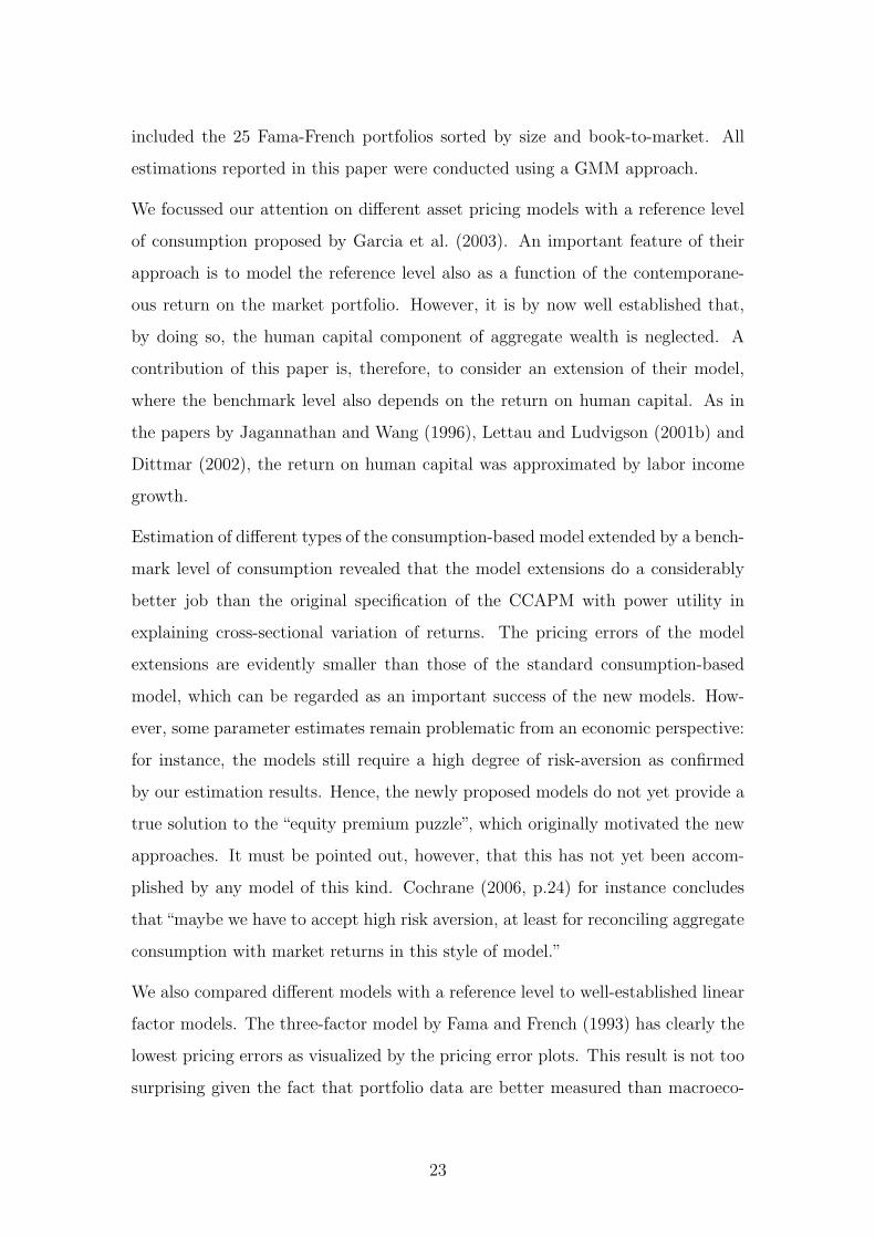
Figure 2: Consumption-based Asset Pricing Models and Benchmark Linear FactorModels: Fitted vs. Actual Mean Returns (in % per quarter). Sample period:

1952:Q2-2002:Q1.

Note: The graphs are based on first-stage GMM estimates using the 25 Fama-French portfolios as test assets.Realized mean returns are given on the horizontal axis, and the returns predicted by the model are provided onthe vertical axis. The first digit represents the size quintiles (1=small, 5=big), whereas the second digit refersto the book-to-market quintiles (1=low, 5=big). The sample period is 1952:Q2-2002:Q1. The upper two graphsshow results for the nonlinear consumption-based model with power utility [RMSE: 0.60%] and the Capital AssetPricing Model [CAPM, RMSE: 0.60%]. Below we display the Garcia-Renault-Semenov model [RMSE: 0.51%] andits Human Capital Extension [RMSE: 0.38%]. At the bottom the plots for the scaled CCAPM by Lettau andLudvigson (2001b) [RMSE: 0.41%] and the Fama-French model [RMSE, 0.32%] are shown.

15

write

Ct+1 =a

ρ+ ρ

∞∑i=0

(1− ρ)iCt−i + εt+1, (12)

where εt+1 denotes an orthogonal innovation. A Koyck-transformation then leads

to the following MA(1) representation:

∆Ct+1 = a− (1− ρ)εt + εt+1. (13)

We follow Garcia et al. (2003) and employ a two-step estimation procedure which

entails estimation of the MA(1) parameters a and ρ in the first step. Using the

estimated parameters one can then construct an estimated habit growth sequence

{Xt+1/Xt} which, in the second step, can then be used to estimate the SDF pa-

rameters by GMM as usual.

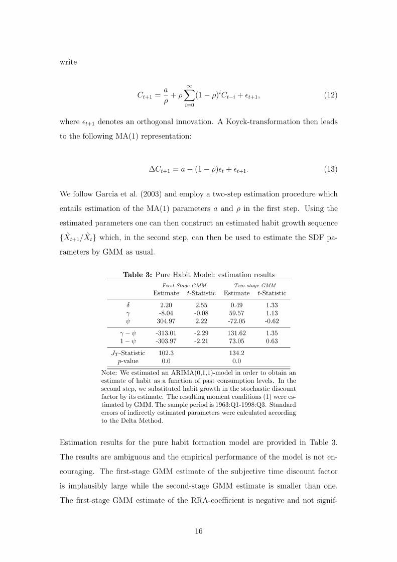
Table 3: Pure Habit Model: estimation resultsFirst-Stage GMM Two-stage GMM


δ 2.20 2.55 0.49 1.33γ -8.04 -0.08 59.57 1.13ψ 304.97 2.22 -72.05 -0.62

γ − ψ -313.01 -2.29 131.62 1.351− ψ -303.97 -2.21 73.05 0.63


Note: We estimated an ARIMA(0,1,1)-model in order to obtain anestimate of habit as a function of past consumption levels. In thesecond step, we substituted habit growth in the stochastic discountfactor by its estimate. The resulting moment conditions (1) were es-timated by GMM. The sample period is 1963:Q1-1998:Q3. Standarderrors of indirectly estimated parameters were calculated accordingto the Delta Method.

Estimation results for the pure habit formation model are provided in Table 3.

The results are ambiguous and the empirical performance of the model is not en-

couraging. The first-stage GMM estimate of the subjective time discount factor

is implausibly large while the second-stage GMM estimate is smaller than one.

The first-stage GMM estimate of the RRA-coefficient is negative and not signif-

16

icantly different from zero, while the second-stage GMM estimate is again quite

large. Based on the first-stage GMM results, the hypotheses ψ = γ and ψ = 1,

respectively, are both rejected at conventional significance levels. This could be in-

terpreted as empirical evidence against the power-utility specification and against

the hypothesis that the reference level does not directly affect the utility of the in-

vestor. However, based on the second-stage GMM results, both hypotheses cannot

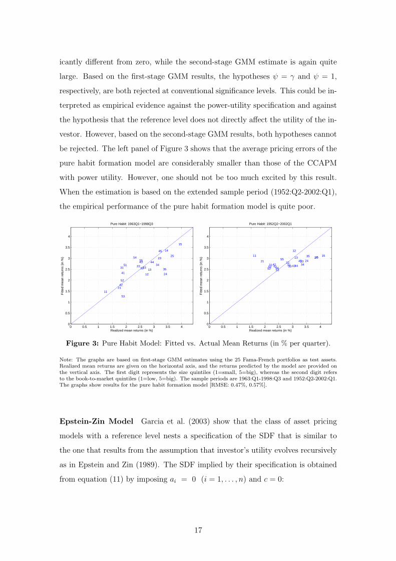
be rejected. The left panel of Figure 3 shows that the average pricing errors of the

pure habit formation model are considerably smaller than those of the CCAPM

with power utility. However, one should not be too much excited by this result.

When the estimation is based on the extended sample period (1952:Q2-2002:Q1),

the empirical performance of the pure habit formation model is quite poor.

0 0.5 1 1.5 2 2.5 3 3.5 40

0.5

1

1.5

2

2.5

3

3.5

4

11

12

13

14

15

21

22

23

24

25

31 323334

3541

42

43 44

45

51

52

53

5455

Pure Habit: 1963Q1−1998Q3

Fitt

ed m

ean

retu

rns

(in %

)


0

0.5

1

1.5

2

2.5

3

3.5

4

11

12

13 1415

21 22 23 2425

31 323334

35

4142 4344

45

5152 5354

55

Pure Habit: 1952Q2−2002Q1

Fitt

ed m

ean

retu

rns

(in %

)


Figure 3: Pure Habit Model: Fitted vs. Actual Mean Returns (in % per quarter).

Note: The graphs are based on first-stage GMM estimates using the 25 Fama-French portfolios as test assets.Realized mean returns are given on the horizontal axis, and the returns predicted by the model are provided onthe vertical axis. The first digit represents the size quintiles (1=small, 5=big), whereas the second digit refersto the book-to-market quintiles (1=low, 5=big). The sample periods are 1963:Q1-1998:Q3 and 1952:Q2-2002:Q1.The graphs show results for the pure habit formation model [RMSE: 0.47%, 0.57%].

Epstein-Zin Model Garcia et al. (2003) show that the class of asset pricing

models with a reference level nests a specification of the SDF that is similar to

the one that results from the assumption that investor’s utility evolves recursively

as in Epstein and Zin (1989). The SDF implied by their specification is obtained

from equation (11) by imposing ai = 0 (i = 1, . . . , n) and c = 0:

17

Mt+1 = δ∗(

Ct+1

Ct

)−γ (Rm

t+1

)κ, (14)

where δ∗ = δ · exp[a0(γ − ψ)] and κ = b(γ − ψ). Conceiving the Epstein-Zin

specification as a special case of an asset pricing model with a reference level one

can write

∆ct+1 = a0 + b · rmt+1 + εt+1, (15)

where rmt+1 denotes the log return of the market portfolio proxy. For parameter

estimation we follow Garcia et al. (2003) and include as instruments for the estima-

tion of equation (15) the log market return and the log consumption growth lagged

by two periods. The resulting moment conditions augment the standard moment

conditions implied by the Epstein-Zin SDF such that all model parameters can be

estimated simultaneously by GMM.

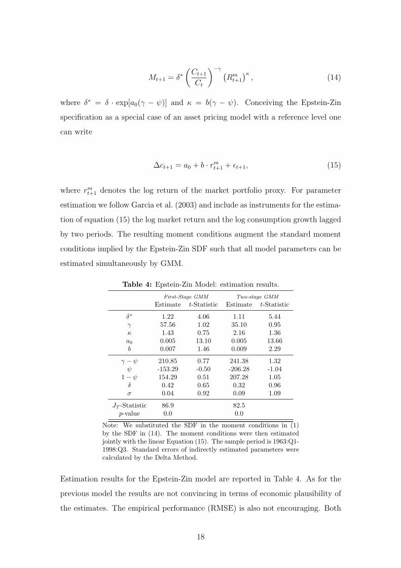
Table 4: Epstein-Zin Model: estimation results.

First-Stage GMM Two-stage GMM


δ∗ 1.22 4.06 1.11 5.44γ 57.56 1.02 35.10 0.95κ 1.43 0.75 2.16 1.36a0 0.005 13.10 0.005 13.66b 0.007 1.46 0.009 2.29

γ − ψ 210.85 0.77 241.38 1.32ψ -153.29 -0.50 -206.28 -1.04

1− ψ 154.29 0.51 207.28 1.05δ 0.42 0.65 0.32 0.96σ 0.04 0.92 0.09 1.09


Note: We substituted the SDF in the moment conditions in (1)by the SDF in (14). The moment conditions were then estimatedjointly with the linear Equation (15). The sample period is 1963:Q1-1998:Q3. Standard errors of indirectly estimated parameters werecalculated by the Delta Method.

Estimation results for the Epstein-Zin model are reported in Table 4. As for the

previous model the results are not convincing in terms of economic plausibility of

the estimates. The empirical performance (RMSE) is also not encouraging. Both

18

first- and second-stage GMM estimates of the RRA coefficient γ are quite large,

but not different from zero at conventional levels of significance. The estimate

of the subjective discount factor δ is implausibly small from an economic point

of view. The hypothesis κ = 0 (or σ = 1/γ) cannot be rejected at conventional

significance levels. Furthermore, neither the hypothesis ψ = γ, nor ψ = 1 can

be rejected. Figure C.1 shows that the empirical performance of the Epstein-Zin

specification in explaining the cross-sectional variation in stock returns remains

unsatisfactory.

Garcia-Renault-Semenov Model In the following we consider a model in

which the growth rate of the reference level is assumed to be a function of the

current period market portfolio log return rmt+1 and log consumption growth lagged

by one period. This implies:

∆ct+1 = a0 + a1 ·∆ct + b · rmt+1 + εt+1. (16)

The SDF of this specification results as a special case of equation (11) by setting

ai = 0 (i = 2, . . . , n); c = 0:

Mt+1 = δ∗(

Ct+1

Ct

)−γ (Ct

Ct−1

)κa1b (

Rmt+1

)κ, (17)

where Rm denotes the market portfolio gross return. We refer to this specification

as the Garcia-Renault-Semenov (GRS) model. The estimation strategy is anal-

ogous to the one pursued for the Epstein-Zin specification. The instruments to

estimate the parameters in equation (16) are a constant and two period lagged

consumption growth and log-market return.10

The estimation results for the GRS model are reported in Table 5. Again, the

results do not make a strong case for asset pricing models with a reference level.

We obtain the familiar CCAPM result that the first-stage estimate of the RRA

10Garcia et al. (2003) suggest to lag the instruments by two periods, arguing that ∆ct mightbe correlated with the innovation εt+1.

19

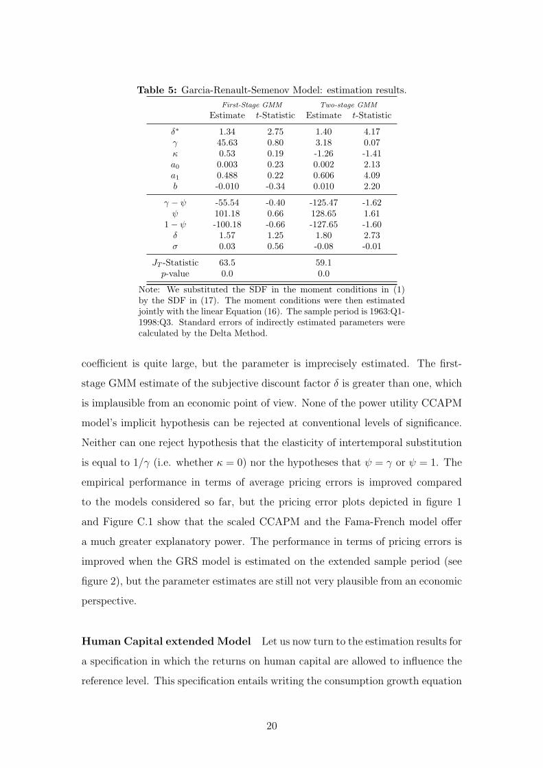
Table 5: Garcia-Renault-Semenov Model: estimation results.First-Stage GMM Two-stage GMM


δ∗ 1.34 2.75 1.40 4.17γ 45.63 0.80 3.18 0.07κ 0.53 0.19 -1.26 -1.41a0 0.003 0.23 0.002 2.13a1 0.488 0.22 0.606 4.09b -0.010 -0.34 0.010 2.20

γ − ψ -55.54 -0.40 -125.47 -1.62ψ 101.18 0.66 128.65 1.61

1− ψ -100.18 -0.66 -127.65 -1.60δ 1.57 1.25 1.80 2.73σ 0.03 0.56 -0.08 -0.01



coefficient is quite large, but the parameter is imprecisely estimated. The first-

stage GMM estimate of the subjective discount factor δ is greater than one, which

is implausible from an economic point of view. None of the power utility CCAPM

model’s implicit hypothesis can be rejected at conventional levels of significance.

Neither can one reject hypothesis that the elasticity of intertemporal substitution

is equal to 1/γ (i.e. whether κ = 0) nor the hypotheses that ψ = γ or ψ = 1. The

empirical performance in terms of average pricing errors is improved compared

to the models considered so far, but the pricing error plots depicted in figure 1

and Figure C.1 show that the scaled CCAPM and the Fama-French model offer

a much greater explanatory power. The performance in terms of pricing errors is

improved when the GRS model is estimated on the extended sample period (see

figure 2), but the parameter estimates are still not very plausible from an economic

perspective.

Human Capital extended Model Let us now turn to the estimation results for

a specification in which the returns on human capital are allowed to influence the

reference level. This specification entails writing the consumption growth equation

20

as

∆ct+1 = a0 + a1 ·∆ct + b · rmt+1 + c · rhc

t+1 + εt+1. (18)

where rhct+1 denotes the log return on human capital in period t + 1. We follow Ja-

gannathan and Wang (1996) and Lettau and Ludvigson (2001b) and approximate

rhc by log labor income growth. Assuming that ai = 0 (i = 2, . . . , n), the SDF

in equation (11) reduces to

Mt+1 = δ∗(

Ct+1

Ct

)−γ (Ct

Ct−1

)κa1b (

Rmt+1

)κ (Rhc

t+1

)κcb , (19)

where Rm denotes the gross return on human capital. We refer to this specification

as the human capital (HC-)extended model. Joint estimation of the parameters in

equations (18) and (19) is performed analogously to the previously discussed two

model specifications (Epstein-Zin and GRS).

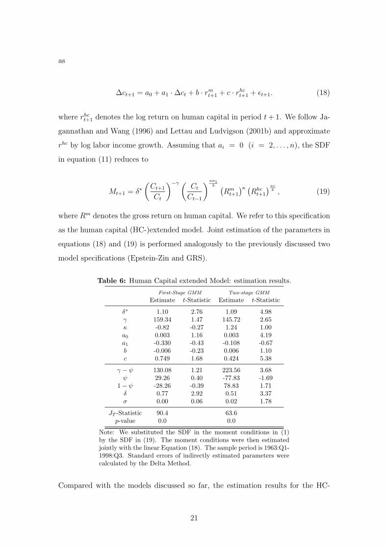
Table 6: Human Capital extended Model: estimation results.



δ∗ 1.10 2.76 1.09 4.98γ 159.34 1.47 145.72 2.65κ -0.82 -0.27 1.24 1.00a0 0.003 1.16 0.003 4.19a1 -0.330 -0.43 -0.108 -0.67b -0.006 -0.23 0.006 1.10c 0.749 1.68 0.424 5.38

γ − ψ 130.08 1.21 223.56 3.68ψ 29.26 0.40 -77.83 -1.69

1− ψ -28.26 -0.39 78.83 1.71δ 0.77 2.92 0.51 3.37σ 0.00 0.06 0.02 1.78



Compared with the models discussed so far, the estimation results for the HC-

21

extended model provided in Table 6 are more sensible from an economic point of

view. Furthermore, the empirical performance in terms of average pricing errors

is encouraging. The estimates of the RRA coefficient are large and imprecise

but we have got used to that in consumption-based asset pricing. Unlike for the

other models discussed so far, the estimates of the subjective time discount factor

are economically more plausible. As a matter of fact, the HC extended model

is the first specification which rejects the restrictions of the CCAPM with power

utility (which motivated the introduction of the model class in the first place).

While the hypothesis that the elasticity of intertemporal substitution is equal to

inverse of the RRA coefficient (κ = 0) cannot be rejected, the second-stage GMM

estimates provide evidence against the CCAPM with power utility in that the

hypothesis that ψ = γ is rejected at conventional significance levels. As evinced

by Figure 1, the HC-extended model accounts quite well for the cross-sectional

variation in the returns of the 25 Fama-French portfolios. The specification delivers

the smallest average pricing errors of all models with a nonlinear SDF. For the

base sample period, the RMSE implied by the HC-extended model is about in

the same range as the RMSE of the scaled CCAPM (scaled CAPM) by Lettau

and Ludvigson. Estimated on the extended sample period, the HC-extension even

outperforms these celebrated scaled factor models (see Figure 2) in terms of pricing

errors. In fact, for this sample period, which overlaps the internet boom, the HC-

extended model produces average pricing errors that come close to those of the

Fama-French model estimated on its ”home turf”. These results can be regarded

as an encouraging empirical success for consumption based asset pricing models

with a reference level.

5 Conclusion

This paper investigated empirically, whether various types of reference-dependent

asset pricing models are able to improve the performance of the consumption-based

model in explaining the variation in cross-sectional returns. For the estimation of

the models, we used a well-established cross-sectional data set: our test assets

22

included the 25 Fama-French portfolios sorted by size and book-to-market. All

estimations reported in this paper were conducted using a GMM approach.

We focussed our attention on different asset pricing models with a reference level

of consumption proposed by Garcia et al. (2003). An important feature of their

approach is to model the reference level also as a function of the contemporane-

ous return on the market portfolio. However, it is by now well established that,

by doing so, the human capital component of aggregate wealth is neglected. A

contribution of this paper is, therefore, to consider an extension of their model,

where the benchmark level also depends on the return on human capital. As in

the papers by Jagannathan and Wang (1996), Lettau and Ludvigson (2001b) and

Dittmar (2002), the return on human capital was approximated by labor income

growth.

Estimation of different types of the consumption-based model extended by a bench-

mark level of consumption revealed that the model extensions do a considerably

better job than the original specification of the CCAPM with power utility in

explaining cross-sectional variation of returns. The pricing errors of the model

extensions are evidently smaller than those of the standard consumption-based

model, which can be regarded as an important success of the new models. How-

ever, some parameter estimates remain problematic from an economic perspective:

for instance, the models still require a high degree of risk-aversion as confirmed

by our estimation results. Hence, the newly proposed models do not yet provide a

true solution to the “equity premium puzzle”, which originally motivated the new

approaches. It must be pointed out, however, that this has not yet been accom-

plished by any model of this kind. Cochrane (2006, p.24) for instance concludes

that “maybe we have to accept high risk aversion, at least for reconciling aggregate

consumption with market returns in this style of model.”

We also compared different models with a reference level to well-established linear

factor models. The three-factor model by Fama and French (1993) has clearly the

lowest pricing errors as visualized by the pricing error plots. This result is not too

surprising given the fact that portfolio data are better measured than macroeco-

23

nomic data. We found that our model extended by human capital rivals the scaled

linearized CCAPM by Lettau and Ludvigson (2001b) in terms of pricing errors,

which is the more appropriate benchmark since it is also based on macroeconomic

data.

Essential for the empirical performance of the consumption-based asset pricing

framework with a reference level, however, is the integration of human capital into

the portfolio of aggregate wealth. Hence, our paper also corroborates the result

by Dittmar (2002) who finds that the incorporation of human capital into the

stochastic discount factor is very important for pricing the cross-section of stock

returns. What is more, the central question of which macroeconomic risks drive risk

premia remains essentially unanswered by portfolio-based models (Cochrane 2006,

p.6). Representative agent models such as those presented in this paper ultimately

seek such a deeper economic understanding. Our results can therefore be seen as

a motivation that future research in the field of consumption-based asset pricing

could lead us to a yet deeper understanding of the true economic forces behind the

variation of expected returns across assets and over time.

24

References

Abel, A.: 1990, Asset prices under habit formation and catching up with the

Joneses, The American Economic Review 80, 38–42.

Ait-Sahalia, Y., Parker, J. A. and Yogo, M.: 2004, Luxury goods and the equity

premium, Journal of Finance 59, 2959–3004.

Altonji, J. and Segal, L. M.: 1996, Small-sample bias in GMM estimation of

covariance structures, Journal of Business and Economic Statistics 14, 353–

366.

Campbell, J. Y. and Cochrane, J. H.: 1999, By force of habit: A consumption

based explanation of aggregate stock market behavior, Journal of Political

Economy 107(2), 205–251.

Campbell, J. Y. and Cochrane, J. H.: 2000, Explaining the poor performance

of consumption-based asset pricing models, Journal of Finance 55(6), 2863–

2878.

Chen, X. and Ludvigson, S.: 2003, Land of addicts? An empirical investigation of

habit-based asset pricing models. Working paper, New York University.

Cochrane, J. H.: 1996, A cross-sectional test of an investment-based asset pricing

model, Journal of Political Economy 104(3), 572–621.

Cochrane, J. H.: 1997, Where is the market going? Uncertain facts and novel

theories, Federal Reserve Bank of Chicago 23, 36–58.

Cochrane, J. H.: 2006, Financial markets and the real economy. Working paper,

University of Chicago.

Constantinides, G. M.: 1990, Habit formation: A resolution of the equity premium

puzzle, Journal of Political Economy 98(3), 519–543.

Dittmar, R. F.: 2002, Nonlinear pricing kernels, kurtosis preference, and evidence

from the cross section of equity returns, Journal of Finance 57, 369–403.

25

Epstein, L. and Zin, S.: 1989, Substitution, risk aversion, and the temporal be-

havior of consumption growth and asset returns I: A theoretical framework,

Econometrica 57, 937–969.

Epstein, L. and Zin, S.: 1991, Substitution, risk aversion, and the temporal behav-

ior of consumption growth and asset returns: An empirical analysis, Journal

of Political Economy 99, 263–286.

Fama, E. F. and French, K. R.: 1993, Common risk factors in the returns on stocks

and bonds, Journal of Financial Economics 33, 3–56.

Ferson, W. E. and Constantinides, G. M.: 1991, Habit persistence and durability

in aggregate consumption; empirical tests, Journal of Financial Economics

29, 199–240.

Garcia, R., Renault, E. and Semenov, A.: 2003, A consumption CAPM with a

reference level. Working paper, Universite de Montreal.

Hall, P. and Horowitz, J.: 1996, Bootstrap critical values for tests based on

generalized-method-of-moments estimators, Econometrica 64, 1517–1527.

Hansen, L. P.: 1982, Large sample properties of generalized method of moments

estimators, Econometrica 50(4), 1029–1054.

Hansen, L. P. and Singleton, K. J.: 1982, Generalized instrumental variables esti-

mation of nonlinear rational expectations models, Econometrica 50(2), 1296–

1286.

Jagannathan, R. and Wang, Z.: 1996, The conditional CAPM and the cross-section

of expected returns, Journal of Finance 51(1), 3–53.

Lettau, M. and Ludvigson, S.: 2001a, Consumption, aggregate wealth, and ex-

pected stock returns, Journal of Finance 56(3), 815–849.

Lettau, M. and Ludvigson, S.: 2001b, Ressurrecting the (C)CAPM: A cross-

sectional test when risk premia are time-varying, Journal of Political Economy

109, 1238–1287.

26

Mehra, R.: 2003, The equity premium: Why is it a puzzle?, Financial Analysts

Journal pp. 54–69.

Mehra, R. and Prescott, E.: 1985, The equity premium: A puzzle, Journal of

Monetary Economics 15, 145–161.

Mehra, R. and Prescott, E.: 2001, The equity premium puzzle in retrospect, in

G. Constantinides, M. Harris and R. Stulz (eds), Handbook of the Economics

of Finance, North Holland.

Parker, J. A. and Julliard, C.: 2005, Consumption risk and the cross section of

expected returns, Journal of Political Economy 113, 185–222.

Piazzesi, M., Schneider, M. and Tuzel, S.: 2006, Housing, consumption and asset

prices. Journal of Financial Economics (forthcoming).

Roll, R. W.: 1977, A critique of the asset pricing theory’s tests, Journal of Finan-

cial Economics 4, 129–176.

Yogo, M.: 2006, A consumption-based explanation of expected stock returns. Jour-

nal of Finance (forthcoming).

27

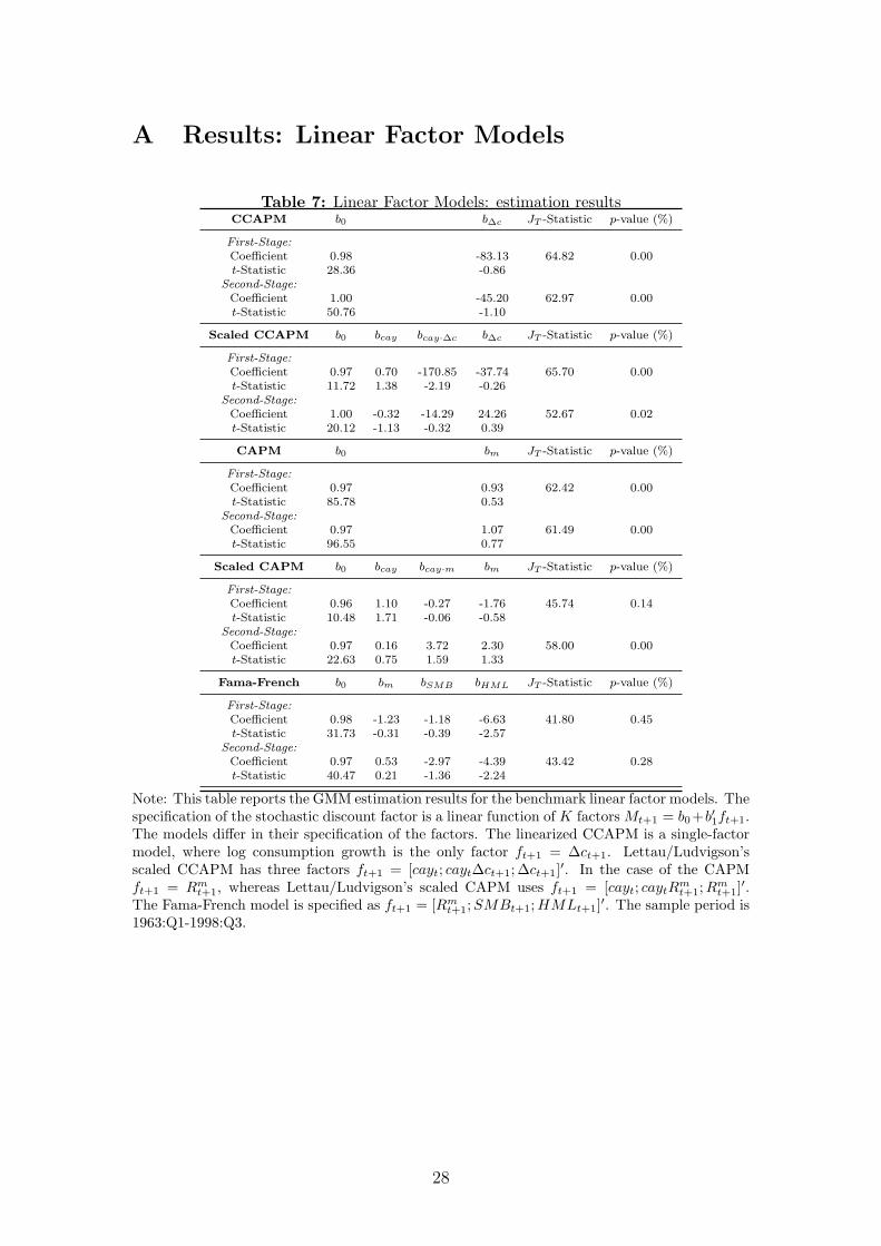
A Results: Linear Factor Models

Table 7: Linear Factor Models: estimation resultsCCAPM b0 b∆c JT -Statistic p-value (%)

First-Stage:Coefficient 0.98 -83.13 64.82 0.00t-Statistic 28.36 -0.86

Second-Stage:Coefficient 1.00 -45.20 62.97 0.00t-Statistic 50.76 -1.10

Scaled CCAPM b0 bcay bcay·∆c b∆c JT -Statistic p-value (%)

First-Stage:Coefficient 0.97 0.70 -170.85 -37.74 65.70 0.00t-Statistic 11.72 1.38 -2.19 -0.26

Second-Stage:Coefficient 1.00 -0.32 -14.29 24.26 52.67 0.02t-Statistic 20.12 -1.13 -0.32 0.39

CAPM b0 bm JT -Statistic p-value (%)

First-Stage:Coefficient 0.97 0.93 62.42 0.00t-Statistic 85.78 0.53

Second-Stage:Coefficient 0.97 1.07 61.49 0.00t-Statistic 96.55 0.77

Scaled CAPM b0 bcay bcay·m bm JT -Statistic p-value (%)


Second-Stage:Coefficient 0.97 0.16 3.72 2.30 58.00 0.00t-Statistic 22.63 0.75 1.59 1.33

Fama-French b0 bm bSMB bHML JT -Statistic p-value (%)

First-Stage:Coefficient 0.98 -1.23 -1.18 -6.63 41.80 0.45t-Statistic 31.73 -0.31 -0.39 -2.57

Second-Stage:Coefficient 0.97 0.53 -2.97 -4.39 43.42 0.28t-Statistic 40.47 0.21 -1.36 -2.24

Note: This table reports the GMM estimation results for the benchmark linear factor models. Thespecification of the stochastic discount factor is a linear function of K factors Mt+1 = b0+b′1ft+1.The models differ in their specification of the factors. The linearized CCAPM is a single-factormodel, where log consumption growth is the only factor ft+1 = ∆ct+1. Lettau/Ludvigson’sscaled CCAPM has three factors ft+1 = [cayt; cayt∆ct+1;∆ct+1]′. In the case of the CAPMft+1 = Rm

t+1, whereas Lettau/Ludvigson’s scaled CAPM uses ft+1 = [cayt; caytRmt+1; R

mt+1]

′.The Fama-French model is specified as ft+1 = [Rm

t+1;SMBt+1; HMLt+1]′. The sample period is1963:Q1-1998:Q3.

28

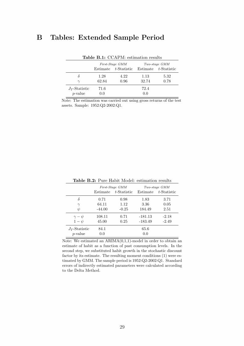
B Tables: Extended Sample Period

Table B.1: CCAPM: estimation resultsFirst-Stage GMM Two-stage GMM


δ 1.28 4.22 1.13 5.32γ 62.84 0.96 32.74 0.78


Note: The estimation was carried out using gross returns of the testassets. Sample: 1952:Q2-2002:Q1.

Table B.2: Pure Habit Model: estimation resultsFirst-Stage GMM Two-stage GMM


δ 0.71 0.98 1.83 3.71γ 64.11 1.12 3.36 0.05ψ -44.00 -0.25 184.49 2.51

γ − ψ 108.11 0.71 -181.13 -2.181− ψ 45.00 0.25 -183.49 -2.49


Note: We estimated an ARIMA(0,1,1)-model in order to obtain anestimate of habit as a function of past consumption levels. In thesecond step, we substituted habit growth in the stochastic discountfactor by its estimate. The resulting moment conditions (1) were es-timated by GMM. The sample period is 1952:Q2-2002:Q1. Standarderrors of indirectly estimated parameters were calculated accordingto the Delta Method.

29

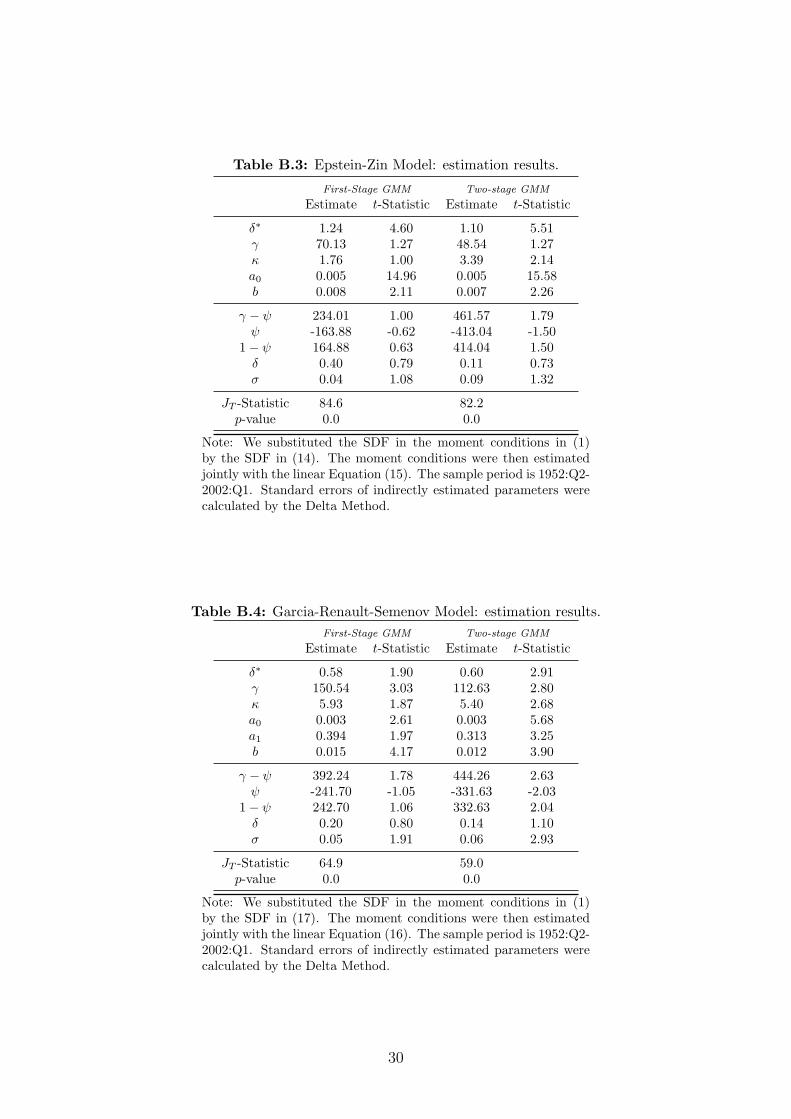
Table B.3: Epstein-Zin Model: estimation results.



δ∗ 1.24 4.60 1.10 5.51γ 70.13 1.27 48.54 1.27κ 1.76 1.00 3.39 2.14a0 0.005 14.96 0.005 15.58b 0.008 2.11 0.007 2.26

γ − ψ 234.01 1.00 461.57 1.79ψ -163.88 -0.62 -413.04 -1.50

1− ψ 164.88 0.63 414.04 1.50δ 0.40 0.79 0.11 0.73σ 0.04 1.08 0.09 1.32



Table B.4: Garcia-Renault-Semenov Model: estimation results.First-Stage GMM Two-stage GMM


δ∗ 0.58 1.90 0.60 2.91γ 150.54 3.03 112.63 2.80κ 5.93 1.87 5.40 2.68a0 0.003 2.61 0.003 5.68a1 0.394 1.97 0.313 3.25b 0.015 4.17 0.012 3.90

γ − ψ 392.24 1.78 444.26 2.63ψ -241.70 -1.05 -331.63 -2.03

1− ψ 242.70 1.06 332.63 2.04δ 0.20 0.80 0.14 1.10σ 0.05 1.91 0.06 2.93



30

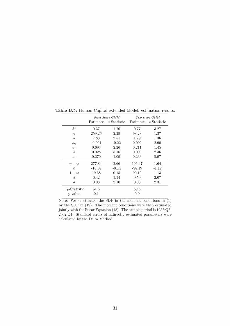
Table B.5: Human Capital extended Model: estimation results.



δ∗ 0.37 1.76 0.77 3.27γ 259.26 2.29 98.28 1.37κ 7.83 2.51 1.79 1.36a0 -0.001 -0.22 0.002 2.90a1 0.693 2.26 0.211 1.45b 0.028 5.16 0.009 2.36c 0.270 1.09 0.233 5.97

γ − ψ 277.84 2.66 196.47 1.64ψ -18.58 -0.14 -98.19 -1.12

1− ψ 19.58 0.15 99.19 1.13δ 0.42 1.54 0.50 2.07σ 0.03 2.10 0.03 2.31



31

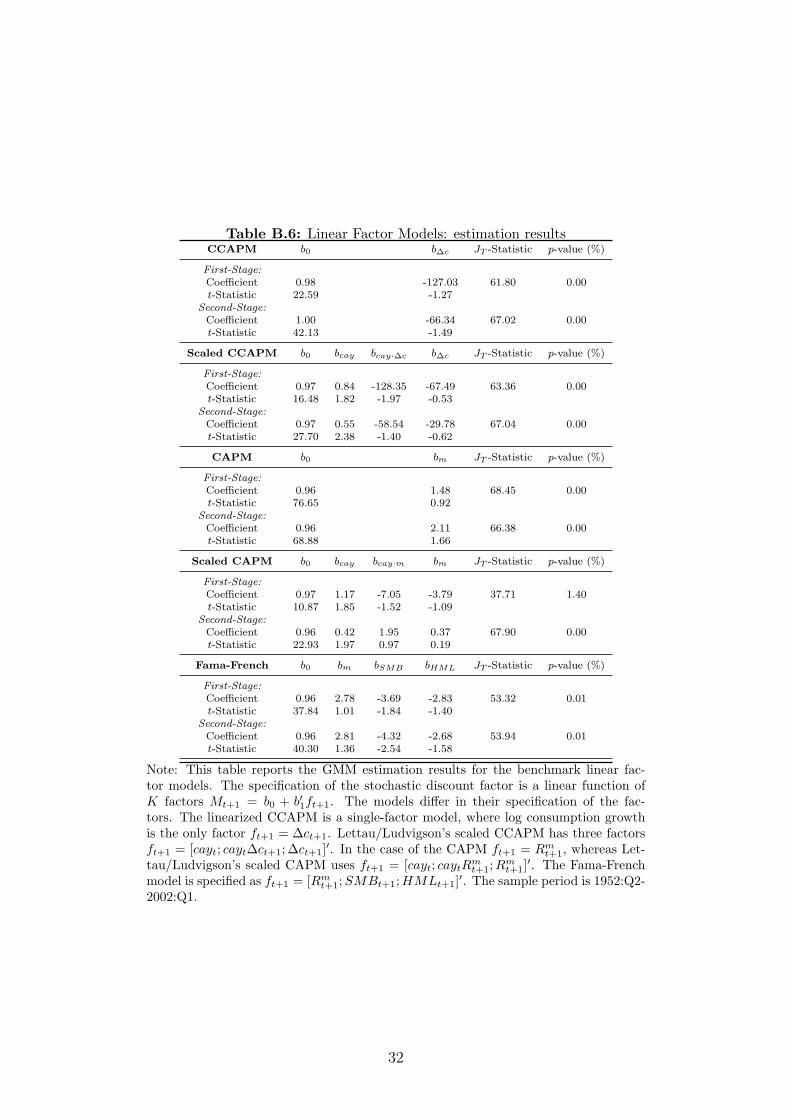
Table B.6: Linear Factor Models: estimation resultsCCAPM b0 b∆c JT -Statistic p-value (%)

First-Stage:Coefficient 0.98 -127.03 61.80 0.00t-Statistic 22.59 -1.27

Second-Stage:Coefficient 1.00 -66.34 67.02 0.00t-Statistic 42.13 -1.49

Scaled CCAPM b0 bcay bcay·∆c b∆c JT -Statistic p-value (%)



CAPM b0 bm JT -Statistic p-value (%)

First-Stage:Coefficient 0.96 1.48 68.45 0.00t-Statistic 76.65 0.92

Second-Stage:Coefficient 0.96 2.11 66.38 0.00t-Statistic 68.88 1.66

Scaled CAPM b0 bcay bcay·m bm JT -Statistic p-value (%)


Second-Stage:Coefficient 0.96 0.42 1.95 0.37 67.90 0.00t-Statistic 22.93 1.97 0.97 0.19

Fama-French b0 bm bSMB bHML JT -Statistic p-value (%)



Note: This table reports the GMM estimation results for the benchmark linear fac-tor models. The specification of the stochastic discount factor is a linear function ofK factors Mt+1 = b0 + b′1ft+1. The models differ in their specification of the fac-tors. The linearized CCAPM is a single-factor model, where log consumption growthis the only factor ft+1 = ∆ct+1. Lettau/Ludvigson’s scaled CCAPM has three factorsft+1 = [cayt; cayt∆ct+1;∆ct+1]′. In the case of the CAPM ft+1 = Rm

t+1, whereas Let-tau/Ludvigson’s scaled CAPM uses ft+1 = [cayt; caytR

mt+1;R

mt+1]

′. The Fama-Frenchmodel is specified as ft+1 = [Rm

t+1; SMBt+1; HMLt+1]′. The sample period is 1952:Q2-2002:Q1.

32

C Additional Figures

0 0.5 1 1.5 2 2.5 3 3.5 40

0.5

1

1.5

2

2.5

3

3.5

4

11

121314 15

2122

23 2425

31

3233 34

35

4142 43 44

455152

53

54

55

Epstein−Zin Model: 1963Q1−1998Q3

Fitt

ed m

ean

retu

rns

(in %

)


0

0.5

1

1.5

2

2.5

3

3.5

4

11

121314 15

21

22

23 2425

31

32

33 3435

41

4243

4445

5152

5354

55

Epstein−Zin Model: 1952Q2−2002Q1

Fitt

ed m

ean

retu

rns

(in %

)


0 0.5 1 1.5 2 2.5 3 3.5 40

0.5

1

1.5

2

2.5

3

3.5

4

1112

13 14 15

21

22 23 24

25

31

32

3334

35

41

42

43

4445

5152 53

5455

Scaled CAPM: 1952Q2−2002Q1

Fitt

ed m

ean

retu

rns

(in %

)


0

0.5

1

1.5

2

2.5

3

3.5

4

11

1213

14

15

21

22

23

24

25

31

32

33 34

35

4142

43 44

45

51

5253

54

55

Scaled CAPM: 1963Q1−1998Q3F

itted

mea

n re

turn

s (in

%)


Figure C.1: Additional Plots: Fitted vs. Actual Mean Returns (in % per quarter).

Note: This figure displays plots for all models not shown in the main text. Realized meanreturns are given on the horizontal axis, and the returns predicted by the model are providedon the vertical axis. The first digit represents the size quintiles (1=small, 5=big), whereasthe second digit refers to the book-to-market quintiles (1=low,5=big). The sample periods are1963:Q1-1998:Q3 and 1952:Q2-2002:Q1. The upper two graphs show results for the pure habitformation model [RMSE: 0.47%(1963:Q1-1998:Q3), 0.57%(1952:Q2-2002:Q1)]. Below we dis-play the Epstein-Zin model [RMSE: 0.66%(1963:Q1-1998:Q3), 0.56%(1952:Q2-2002:Q1)]. At thebottom the plots for the scaled CAPM by Lettau and Ludvigson (2001b) [RMSE: 0.58%(1963:Q1-1998:Q3), 0.43%(1952:Q2-2002:Q1)] are shown.

33

Documents

Consumption-Based Asset Pricing with a Reference …ftp.zew.de/pub/zew-docs/dp/dp0632.pdf · Consumption-Based Asset Pricing with a Reference Level: New Evidence from the ... According