Embed Size (px)
Citation preview
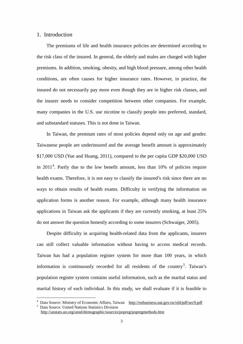
Marital Status as a Risk Factor in Life Insurance: An Empirical Study in Taiwan
Hsin Chung Wang1 Jack C. Yue2 Yi-Hsuan Tsai3
Abstract
Gender and age are the top two risk factors considered in pricing life insurance
products. Although it is believed that mortality rates are also related to other factors
(e.g., smoking, overweight, and especially marriage), data availability and marketing
often limit the possibility of including them. Many studies have shown that married
people (particularly men) benefit from the marriage, and generally have lower
mortality rates than unmarried people. However, most of these studies used data from
a population sample; their results might not apply to the whole population. In this
study, we explore if mortality rates differ by marital status using mortality data (1975–
2011) from the Taiwan Ministry of the Interior.
In order to deal with the problem of small sample sizes in some marital status
groups, we use graduation methods to reduce fluctuations in mortality rates. We also
use a relational approach to model mortality rates by marital status, and then compare
the proposed model with some popular stochastic mortality models. Based on
computer simulation, we find that the proposed smoothing methods can reduce
fluctuations in mortality estimates between ages, and the relational mortality model
has smaller errors in predicting mortality rates by marital status. Analyses of the
mortality data from Taiwan show that mortality rates differ significantly by marital
1 Assistant Professor, Department of Finance and Actuarial Science, Aletheia University, New Taipei
City, Taiwan, Republic of China 2 Professor, Department of Statistics, National Chengchi University, Taipei, Taiwan, Republic of China 3 Master, Department of Risk Management and Insurance, National Chengchi University, Taipei,
Taiwan, Republic of China

2
status. In some age groups, the differences in mortality rates are larger between marital
status groups than between smokers and non-smokers. For the issue of practical
consideration, we suggest modifications to include marital status in pricing of life
insurance products.
Key Words: Marital Status, Risk Factor, Small Area Estimation, Longevity Risk,
Relational Mortality Model
3
1. Introduction
The premiums of life and health insurance policies are determined according to
the risk class of the insured. In general, the elderly and males are charged with higher
premiums. In addition, smoking, obesity, and high blood pressure, among other health
conditions, are often causes for higher insurance rates. However, in practice, the
insured do not necessarily pay more even though they are in higher risk classes, and
the insurer needs to consider competition between other companies. For example,
many companies in the U.S. use nicotine to classify people into preferred, standard,
and substandard statuses. This is not done in Taiwan.
In Taiwan, the premium rates of most policies depend only on age and gender.
Taiwanese people are underinsured and the average benefit amount is approximately
$17,000 USD (Yue and Huang, 2011), compared to the per capita GDP $20,000 USD
in 20114. Partly due to the low benefit amount, less than 10% of policies require
health exams. Therefore, it is not easy to classify the insured’s risk since there are no
ways to obtain results of health exams. Difficulty in verifying the information on
application forms is another reason. For example, although many health insurance
applications in Taiwan ask the applicants if they are currently smoking, at least 25%
do not answer the question honestly according to some insurers (Schwaiger, 2005).
Despite difficulty in acquiring health-related data from the applicants, insurers
can still collect valuable information without having to access medical records.
Taiwan has had a population register system for more than 100 years, in which
information is continuously recorded for all residents of the country5. Taiwan’s
population register system contains useful information, such as the marital status and
marital history of each individual. In this study, we shall evaluate if it is feasible to
4 Data Source: Ministry of Economic Affairs, Taiwan http://twbusiness.nat.gov.tw/old/pdf/sec9.pdf 5 Data Source: United Nations Statistics Division
http://unstats.un.org/unsd/demographic/sources/popreg/popregmethods.htm
4
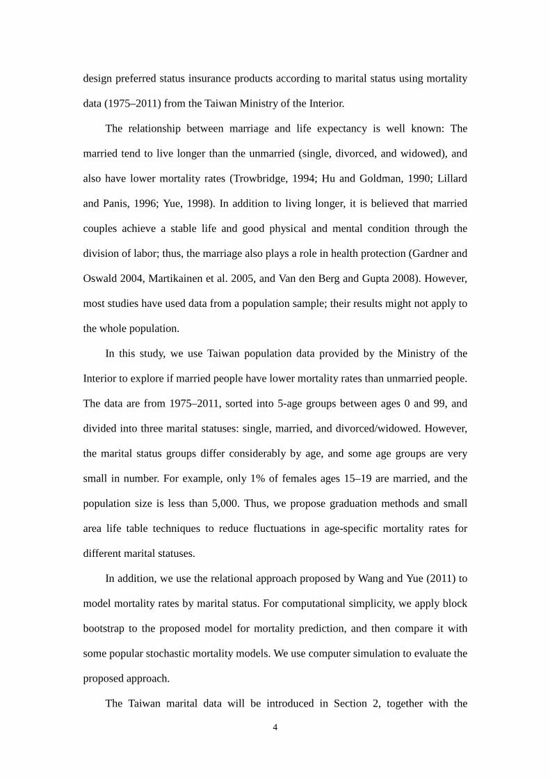
design preferred status insurance products according to marital status using mortality
data (1975–2011) from the Taiwan Ministry of the Interior.
The relationship between marriage and life expectancy is well known: The
married tend to live longer than the unmarried (single, divorced, and widowed), and
also have lower mortality rates (Trowbridge, 1994; Hu and Goldman, 1990; Lillard
and Panis, 1996; Yue, 1998). In addition to living longer, it is believed that married
couples achieve a stable life and good physical and mental condition through the
division of labor; thus, the marriage also plays a role in health protection (Gardner and
Oswald 2004, Martikainen et al. 2005, and Van den Berg and Gupta 2008). However,
most studies have used data from a population sample; their results might not apply to
the whole population.
In this study, we use Taiwan population data provided by the Ministry of the
Interior to explore if married people have lower mortality rates than unmarried people.
The data are from 1975–2011, sorted into 5-age groups between ages 0 and 99, and
divided into three marital statuses: single, married, and divorced/widowed. However,
the marital status groups differ considerably by age, and some age groups are very
small in number. For example, only 1% of females ages 15–19 are married, and the
population size is less than 5,000. Thus, we propose graduation methods and small
area life table techniques to reduce fluctuations in age-specific mortality rates for
different marital statuses.
In addition, we use the relational approach proposed by Wang and Yue (2011) to
model mortality rates by marital status. For computational simplicity, we apply block
bootstrap to the proposed model for mortality prediction, and then compare it with
some popular stochastic mortality models. We use computer simulation to evaluate the
proposed approach.
The Taiwan marital data will be introduced in Section 2, together with the
5
graduation methods (especially for small areas) for the mortality rates by marital
status and the mortality models. In Section 3, a simulation study of graduation
methods is provided first, and then a feasible method is applied to the empirical
analysis of mortality rates by marital status. The differences in age-specific mortality
rates and life expectancy between marital statuses are also calculated. In Section 4, the
proposed mortality approach is applied to model mortality rates by marital status. The
results are compared with popular mortality models, such as the Lee-Carter model
(1992), Renshaw-Haberman model (2006), and the Cairns-Blake-Dowd model (2006).
The final section contains discussions about the study of marital mortality rates and
the practical issue of whether marital status can be treated as a risk factor in life
insurance products.
2. Data and Methodology
Taiwan marital data can be downloaded from the Taiwan Ministry of the Interior6.
Table 1 lists the age ranges of population and death records by marital status since
1973, including the lowest and highest ages recorded.
Table 1. Taiwan’s Population and Death Records with Respect to Marital Status
Year Population (Unit: age)
Deaths (Unit: age)
1973–1974 15–50+ N/A 1975–1991 15–50+ 15–85+ 1992–1993 15–50+ 15–95+ 1994–1997 15–100+ 15–95+ 1998–2011 15–100+ 15–100+
Because detailed mortality records are only available from 1994 on, we compare
6 There are four types of marital status: 1) currently married, and the unmarried, which includes persons who are 2) single (never married), 3) widowed, or 4) divorced. Due to small sample sizes, we combined the divorced and widowed into a single group called divorced/widowed.
6
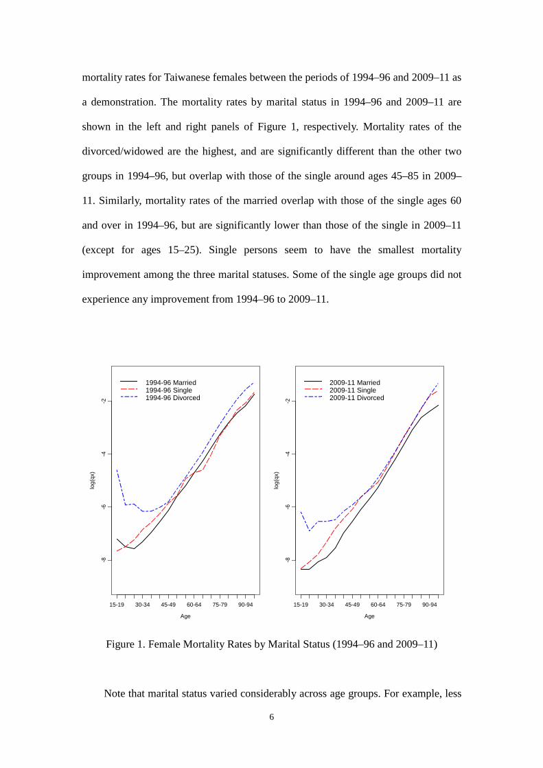
mortality rates for Taiwanese females between the periods of 1994–96 and 2009–11 as
a demonstration. The mortality rates by marital status in 1994–96 and 2009–11 are
shown in the left and right panels of Figure 1, respectively. Mortality rates of the
divorced/widowed are the highest, and are significantly different than the other two
groups in 1994–96, but overlap with those of the single around ages 45–85 in 2009–
11. Similarly, mortality rates of the married overlap with those of the single ages 60
and over in 1994–96, but are significantly lower than those of the single in 2009–11
(except for ages 15–25). Single persons seem to have the smallest mortality
improvement among the three marital statuses. Some of the single age groups did not
experience any improvement from 1994–96 to 2009–11.
Figure 1. Female Mortality Rates by Marital Status (1994–96 and 2009–11)
Note that marital status varied considerably across age groups. For example, less
Age
log(
qx)
15-19 30-34 45-49 60-64 75-79 90-94
-8-6
-4-2
1994-96 Married1994-96 Single1994-96 Divorced
Age
log(
qx)
15-19 30-34 45-49 60-64 75-79 90-94
-8-6
-4-2
2009-11 Married2009-11 Single2009-11 Divorced
7
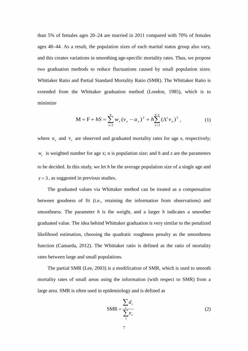
than 5% of females ages 20–24 are married in 2011 compared with 70% of females
ages 40–44. As a result, the population sizes of each marital status group also vary,
and this creates variations in smoothing age-specific mortality rates. Thus, we propose
two graduation methods to reduce fluctuations caused by small population sizes:
Whittaker Ratio and Partial Standard Mortality Ratio (SMR). The Whittaker Ratio is
extended from the Whittaker graduation method (London, 1985), which is to
minimize
∑∑==
∆+−=+=z-n
1x
2n
1
2 )()(FM xz
xxxx vhuvwhS , (1)
where xu and xv
are observed and graduated mortality rates for age x, respectively;
xw is weighted number for age x; n is population size; and h and z are the parameters
to be decided. In this study, we let h be the average population size of a single age and
3=z , as suggested in previous studies.
The graduated values via Whittaker method can be treated as a compensation
between goodness of fit (i.e., retaining the information from observations) and
smoothness. The parameter h is the weight, and a larger h indicates a smoother
graduated value. The idea behind Whittaker graduation is very similar to the penalized
likelihood estimation, choosing the quadratic roughness penalty as the smoothness
function (Camarda, 2012). The Whittaker ratio is defined as the ratio of mortality
rates between large and small populations.
The partial SMR (Lee, 2003) is a modification of SMR, which is used to smooth
mortality rates of small areas using the information (with respect to SMR) from a
large area. SMR is often used in epidemiology and is defined as
∑∑
=
xx
xx
e
dSMR (2)
8
where xd and xe
are the observed and expected numbers of deaths for age x,
respectively. Therefore, an SMR greater than 1 or less than 1 indicates whether an
area has a higher or lower overall mortality rate, respectively. This is why the SMR
can be treated as a mortality index. If the size of a certain age group in the small area
is small, the observed mortality rate would fluctuate considerably. The SMR can be
used, however, to refine the mortality rate.
For the partial SMR, the graduated mortality rates satisfy
−+×
×−+×××=
∑∑
)/1(ˆ)SMRlog()/1()/log(ˆ
exp2
2*
xxx
xxxxxxx ddhd
ddedhduv , (3)
or the weighted average between raw mortality rates and SMR, where 2h is the
estimate of parameter 2h for measuring the heterogeneity (in mortality rates) between
the small area and large area. *xu is the mortality rate for age x in a large area. To
avoid unreasonable results, Lee suggests that
( ).0 ,
)(maxˆ
22
22
×−×−
=∑
∑ ∑x
xxx
eSMRdSMRed
h (4)
The larger 2h is, the larger the difference in age-specific mortality rates (i.e.,
mortality heterogeneity, or larger dissimilarity in shape between the age-specific
mortality curve of the small population and that of the larger population). When the
number of deaths is smaller, there will be greater weight from the large area, and the
graduated value equals *SMR xu×
when the number of deaths is zero.
Graduation is one of the methods for constructing small area life tables. Most of
the graduation methods, such as moving weighted average and Whittaker method, can
be treated as different ways of increasing samples, or reducing the variations of
9
mortality rates based on the information from the small area. On the other hand,
borrowing/combining mortality information with other populations is another way to
reduce the variations of mortality rates in the small area. Many authors use two or
more populations with similar mortality profiles, together with the choice of mortality
models, to stabilize mortality estimates. For example, Dowd et al. (2011) and Jarner
and Kryger (2011) proposed a gravity mortality model and the SAINT model,
respectively, for two related but different-sized populations. Li and Lee (2005) and
Zhou et al. (2013) modified the Lee-Carter model for modeling multiple populations.
Cairns et al. (2011) applied the Age-Period-Cohort model combining Bayesian
methods for the two populations. Partial SMR can be treated as one way of borrowing
information from a large population.
We introduce the proposed mortality model, followed by frequently used
mortality models. Wang and Yue (2011) proposed a relational model (RM) defined by
)()()( 1
tptptr
x
xx
+= , (5)
where )()()( 1
tltltp
x
xx
+=
and xl are survival probability and the life table function,
number of survivors for age x at time t. Wang and Yue suggested using the Brownian
motion stochastic differential equations (BMSDE) and block bootstrap simulation to predict
the values of )(trx .
In addition to the proposed mortality model, we also consider the Lee-Carter (LC)
model (Lee and Carter, 1992), Renshaw-Haberman (RH) model (Renshaw and
Haberman, 2006), and the Cairns-Blake-Dowd (CBD) model (Cairns et al., 2006). If
xtm denotes the central death rate for a person aged x at time t, the LC model
assumes that
txtxxxtm ,)2()2()1()log( εκββ ++= , (6)
10
with two constraints, ∑ =x
x1)2(β
and ∑ =t
t0)2(κ , and the parameter )1(
xβ denotes the
average age-specific mortality; )2(tκ
represents the general mortality level; and the
decline in mortality at age x is captured by )2(xβ . The mortality level )2(
tκ is usually a
linear function in time. The term εx,t denotes the deviation of the model from the
observed log-central death rates and is assumed to be white noise, with 0 mean and
relatively small variance. The parameters of LC model can be estimated via the
singular value decomposition.
Since the residuals of fitting the LC model are not random (Debón et al., 2008),
some studies suggest adding an extra time or cohort component to the LC model. The
RH Model can be treated as a version of LC Model with an extra cohort component,
)3()3()2()2()1()ln( xtxtxxxtm −++= γβκββ , (7)
where ∑∑∑∑ ==== −tx
xtx
xt
tx
x,
)3()3()2()2( 0,1,0,1 γβκβ , and the parameter )(i
xβ ,
3,2,1=i reflects the age-related effects; )2(
tκ reflects period-related effects and
represents the general mortality level; )3(xt−γ
reflects cohort-related effects.
The CBD model is designed to model mortality rates for higher ages, and deal
with the longevity risk in pensions and annuities. For the CBD model, it assumes that
the mortality rates satisfy
logit (𝑞𝑞𝑥𝑥𝑥𝑥) )2()2()1()1(
1log txtx
xt
xt
qq κβκβ +=−
= , (8)
where the parameters are )(ixβ
and )(itκ ; 2,1=i reflects age-related effects and the
general mortality level. If we suppose 1)1( =xβ and xxx −=)2(β , then the model has a
simple parametric form as follows:
11
logit (𝑞𝑞𝑥𝑥𝑥𝑥) )()2()1( xxtt −+= κκ . (9)
3. Marital Status Life Table
As previously mentioned, the population size of each marital status group varies
by age. Thus, we need to look for feasible graduation methods to reduce the
fluctuations in mortality rates. We use computer simulation to study if the graduation
methods of interest (Whittaker, Whittaker Ratio, and Partial SMR) can reduce the
variations of the ungraduated mortality rates. Let the large area be all of Taiwan
(population size: approximately 23 million) and the small area be Pen-Hu county
(population size: about 100,000). We use the male to demonstrate the effect of
graduation. Since Pen-Hu county has only about 50,000 males, the number of elderly
is small. Therefore, 17 age groups are considered in the simulation study: 0–4, 5–9,
10–14, …, 75–79, and >80. Note that the proportions of elderly males (> age 65) and
oldest-old males (> age 85) in Pen-Hu county are 13.5% and 1.1%, both of which are
slightly higher than those in Taiwan (10.0% and 0.8%, respectively).
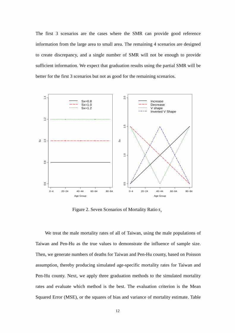
Let sxq
and
Bxq
denote the mortality rates of the small area and large area,
respectively. Suppose these two mortality rates satisfy Bxx
sx qsq ×= and there are 7
possible scenarios for the mortality ratio xs as shown in Figure 2:
8.0=xs
0.1=xs
2.1=xs
xs increases linearly with age
xs decreases linearly with age
xs decreases linearly first and then increases linearly (V-shape)
xs increases linearly first and then decreases linearly (reverse V-shape)
12
The first 3 scenarios are the cases where the SMR can provide good reference
information from the large area to small area. The remaining 4 scenarios are designed
to create discrepancy, and a single number of SMR will not be enough to provide
sufficient information. We expect that graduation results using the partial SMR will be
better for the first 3 scenarios but not as good for the remaining scenarios.
Figure 2. Seven Scenarios of Mortality Ratio xs
We treat the male mortality rates of all of Taiwan, using the male populations of
Taiwan and Pen-Hu as the true values to demonstrate the influence of sample size.
Then, we generate numbers of deaths for Taiwan and Pen-Hu county, based on Poisson
assumption, thereby producing simulated age-specific mortality rates for Taiwan and
Pen-Hu county. Next, we apply three graduation methods to the simulated mortality
rates and evaluate which method is the best. The evaluation criterion is the Mean
Squared Error (MSE), or the squares of bias and variance of mortality estimate. Table
Age Group
Sx
0~4 20~24 40~44 60~64 80~84
0.6
0.8
1.0
1.2
1.4
Sx=0.8Sx=1.0Sx=1.2
Age Group
Sx
0~4 20~24 40~44 60~64 80~84
0.5
1.0
1.5
2.0
IncreaseDecreaseV shapeInverted V Shape
13
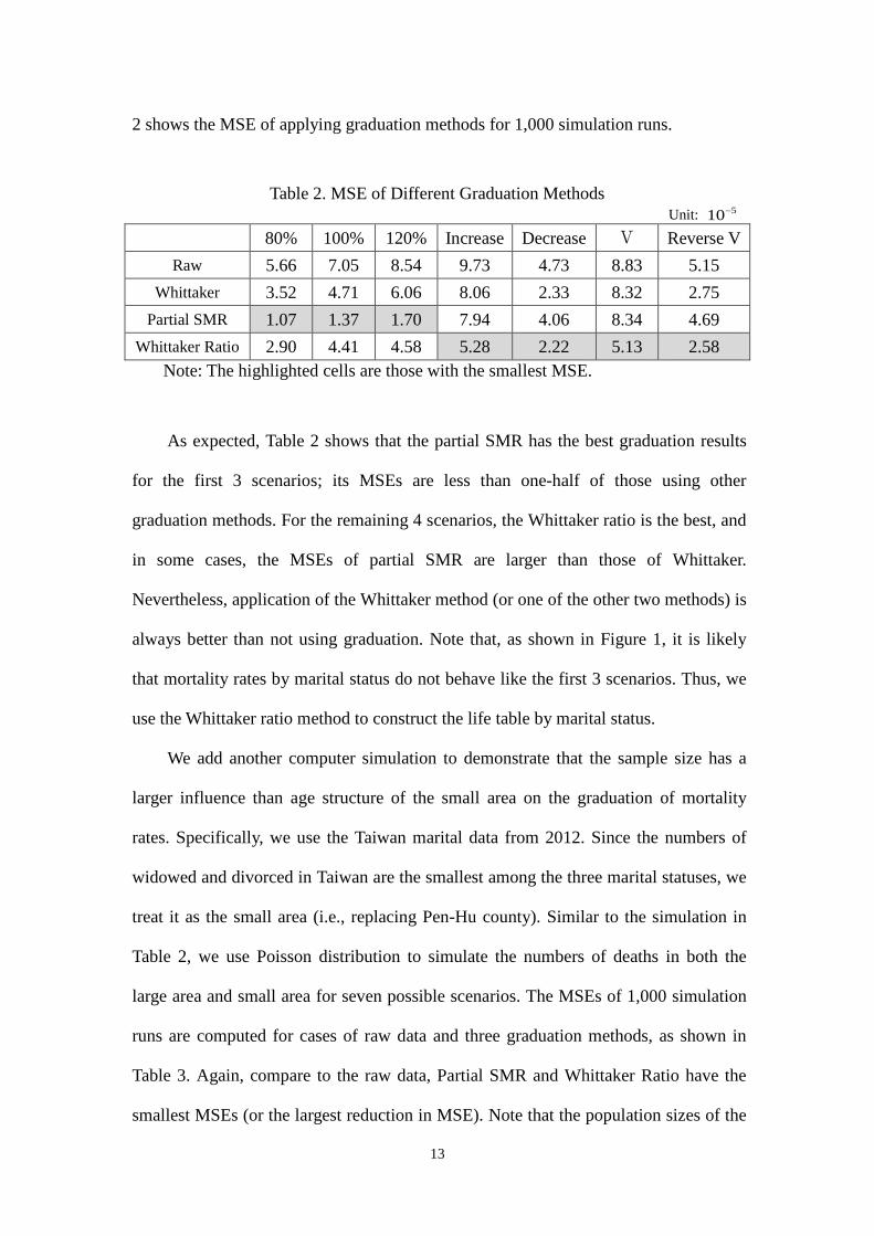
2 shows the MSE of applying graduation methods for 1,000 simulation runs.
Table 2. MSE of Different Graduation Methods Unit: 510−
80% 100% 120% Increase Decrease V Reverse V Raw 5.66 7.05 8.54 9.73 4.73 8.83 5.15
Whittaker 3.52 4.71 6.06 8.06 2.33 8.32 2.75 Partial SMR 1.07 1.37 1.70 7.94 4.06 8.34 4.69
Whittaker Ratio 2.90 4.41 4.58 5.28 2.22 5.13 2.58 Note: The highlighted cells are those with the smallest MSE.
As expected, Table 2 shows that the partial SMR has the best graduation results
for the first 3 scenarios; its MSEs are less than one-half of those using other
graduation methods. For the remaining 4 scenarios, the Whittaker ratio is the best, and
in some cases, the MSEs of partial SMR are larger than those of Whittaker.
Nevertheless, application of the Whittaker method (or one of the other two methods) is
always better than not using graduation. Note that, as shown in Figure 1, it is likely
that mortality rates by marital status do not behave like the first 3 scenarios. Thus, we
use the Whittaker ratio method to construct the life table by marital status.
We add another computer simulation to demonstrate that the sample size has a
larger influence than age structure of the small area on the graduation of mortality
rates. Specifically, we use the Taiwan marital data from 2012. Since the numbers of
widowed and divorced in Taiwan are the smallest among the three marital statuses, we
treat it as the small area (i.e., replacing Pen-Hu county). Similar to the simulation in
Table 2, we use Poisson distribution to simulate the numbers of deaths in both the
large area and small area for seven possible scenarios. The MSEs of 1,000 simulation
runs are computed for cases of raw data and three graduation methods, as shown in
Table 3. Again, compare to the raw data, Partial SMR and Whittaker Ratio have the
smallest MSEs (or the largest reduction in MSE). Note that the population sizes of the
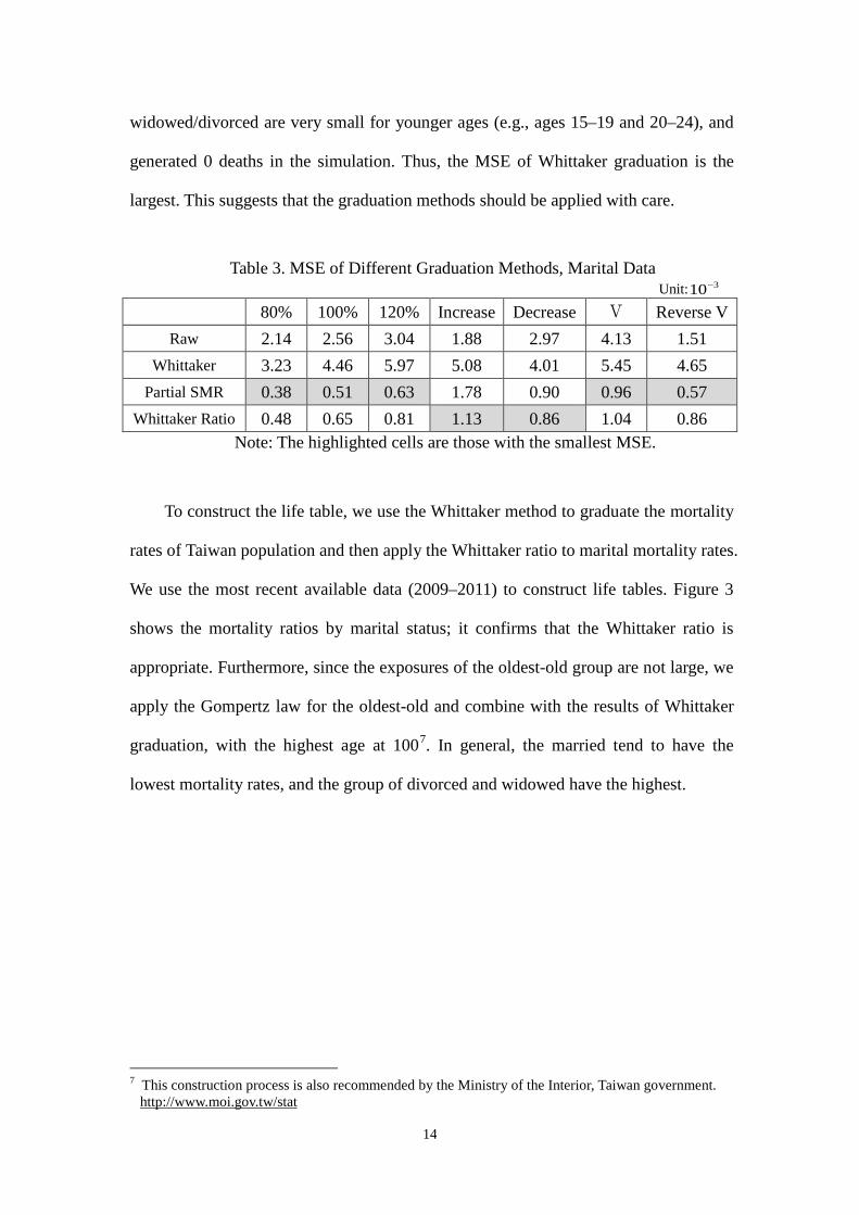
14
widowed/divorced are very small for younger ages (e.g., ages 15–19 and 20–24), and
generated 0 deaths in the simulation. Thus, the MSE of Whittaker graduation is the
largest. This suggests that the graduation methods should be applied with care.
Table 3. MSE of Different Graduation Methods, Marital Data Unit: 310−
80% 100% 120% Increase Decrease V Reverse V Raw 2.14 2.56 3.04 1.88 2.97 4.13 1.51
Whittaker 3.23 4.46 5.97 5.08 4.01 5.45 4.65 Partial SMR 0.38 0.51 0.63 1.78 0.90 0.96 0.57
Whittaker Ratio 0.48 0.65 0.81 1.13 0.86 1.04 0.86 Note: The highlighted cells are those with the smallest MSE.
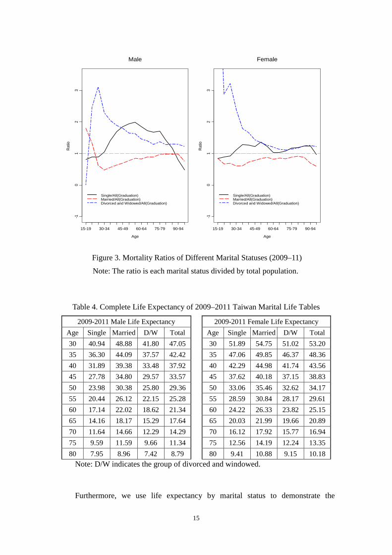
To construct the life table, we use the Whittaker method to graduate the mortality
rates of Taiwan population and then apply the Whittaker ratio to marital mortality rates.
We use the most recent available data (2009–2011) to construct life tables. Figure 3
shows the mortality ratios by marital status; it confirms that the Whittaker ratio is
appropriate. Furthermore, since the exposures of the oldest-old group are not large, we
apply the Gompertz law for the oldest-old and combine with the results of Whittaker
graduation, with the highest age at 1007. In general, the married tend to have the
lowest mortality rates, and the group of divorced and widowed have the highest.
7 This construction process is also recommended by the Ministry of the Interior, Taiwan government.
http://www.moi.gov.tw/stat
15
Figure 3. Mortality Ratios of Different Marital Statuses (2009–11)
Note: The ratio is each marital status divided by total population.
Table 4. Complete Life Expectancy of 2009–2011 Taiwan Marital Life Tables
2009-2011 Male Life Expectancy 2009-2011 Female Life Expectancy Age Single Married D/W Total Age Single Married D/W Total 30 40.94 48.88 41.80 47.05 30 51.89 54.75 51.02 53.20 35 36.30 44.09 37.57 42.42 35 47.06 49.85 46.37 48.36 40 31.89 39.38 33.48 37.92 40 42.29 44.98 41.74 43.56 45 27.78 34.80 29.57 33.57 45 37.62 40.18 37.15 38.83 50 23.98 30.38 25.80 29.36 50 33.06 35.46 32.62 34.17 55 20.44 26.12 22.15 25.28 55 28.59 30.84 28.17 29.61 60 17.14 22.02 18.62 21.34 60 24.22 26.33 23.82 25.15 65 14.16 18.17 15.29 17.64 65 20.03 21.99 19.66 20.89 70 11.64 14.66 12.29 14.29 70 16.12 17.92 15.77 16.94 75 9.59 11.59 9.66 11.34 75 12.56 14.19 12.24 13.35 80 7.95 8.96 7.42 8.79 80 9.41 10.88 9.15 10.18
Note: D/W indicates the group of divorced and windowed.
Furthermore, we use life expectancy by marital status to demonstrate the
Male
Age
Rat
io
15-19 30-34 45-49 60-64 75-79 90-94
-10
12
3
Single/All(Graduation)Married/All(Graduation)Divorced and Widowed/All(Graduation)
Female
Age
Rat
io
15-19 30-34 45-49 60-64 75-79 90-94
-10
12
3
Single/All(Graduation)Married/All(Graduation)Divorced and Widowed/All(Graduation)
16
differences by marital status (Table 4). Since the marital data start at age 15 and the
highest age for constructing life table is age 100, we only compare life expectancy for
ages 30–80. The difference in life expectancy between married and single persons
reach the largest value (almost 8 years) at age 30. This difference is very significant in
pricing life insurance products. The difference is still noticeable for higher age groups
-i.e., at age 65, there is a 4-year difference in life expectancy found between married
and single men.
We compare differences in premiums for pricing life insurance products based on
whethere the insured is married, single, or divorced/widowed. For simplicity, we only
compare the married and single. Premiums are for a 20-year payment whole life policy,
with an interest rate of 2% or 5%, and highest attained age of 100. Although people
can switch between different marital statuses, such as from single to married or from
married to divorced, the results for each cell in Tables 5 and 6 are based on the
assumption that the insured’ marital status stays constant.
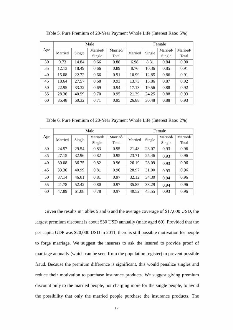
Pure premiums per $1,000 USD coverage are shown in Tables 5 and 6, along
with the premium ratios, and ratios of married per total population. Similar to the
results of life expectancy in Table 4, the married male receives a larger discount in
premium than the single male. Premiums for the married males are discounted by
about 34% at the 5% rate, and by 22% at the 2% rate. The discount rate is slightly less
for the married female at about 16% and 7% for the two interest rates, respectively.
Marital status is a significant factor when compared with premium discounts for
nonsmokers (14% less than smokers) and persons of normal weight (22% less than
obese persons)8.
8 Source: eHealth, Inc.
http://www.marketwatch.com/story/smokers-pay-14-higher-health-insurance-premiums-than-non-smokers-ehealth-data-shows-2013-01-03
17
Table 5. Pure Premium of 20-Year Payment Whole Life (Interest Rate: 5%)
Age Male Female
Married Single Married/ Single
Married/ Total
Married Single Married/ Single
Married/ Total
30 9.73 14.84 0.66 0.88 6.98 8.31 0.84 0.90 35 12.13 18.49 0.66 0.89 8.76 10.36 0.85 0.91 40 15.08 22.72 0.66 0.91 10.99 12.85 0.86 0.91 45 18.64 27.57 0.68 0.93 13.73 15.86 0.87 0.92 50 22.95 33.32 0.69 0.94 17.13 19.56 0.88 0.92 55 28.36 40.59 0.70 0.95 21.39 24.25 0.88 0.93 60 35.48 50.32 0.71 0.95 26.88 30.48 0.88 0.93
Table 6. Pure Premium of 20-Year Payment Whole Life (Interest Rate: 2%)
Age Male Female
Married Single Married/ Single
Married/ Total
Married Single Married/ Single
Married/ Total
30 24.57 29.54 0.83 0.95 21.48 23.07 0.93 0.96 35 27.15 32.96 0.82 0.95 23.71 25.46 0.93 0.96
40 30.08 36.75 0.82 0.96 26.19 28.09 0.93 0.96
45 33.36 40.99 0.81 0.96 28.97 31.00 0.93 0.96
50 37.14 46.01 0.81 0.97 32.12 34.30 0.94 0.96
55 41.78 52.42 0.80 0.97 35.85 38.29 0.94 0.96 60 47.89 61.08 0.78 0.97 40.52 43.55 0.93 0.96
Given the results in Tables 5 and 6 and the average coverage of $17,000 USD, the
largest premium discount is about $30 USD annually (male aged 60). Provided that the
per capita GDP was $20,000 USD in 2011, there is still possible motivation for people
to forge marriage. We suggest the insurers to ask the insured to provide proof of
marriage annually (which can be seen from the population register) to prevent possible
fraud. Because the premium difference is significant, this would penalize singles and
reduce their motivation to purchase insurance products. We suggest giving premium
discount only to the married people, not charging more for the single people, to avoid
the possibility that only the married people purchase the insurance products. The
18
premium discount of the married status is based on the married over the total
population.
4. Modeling Mortality Rates by Marital Status
In the previous section, we report that the married have lower mortality rates than
the unmarried, a statistic that may be used to differentiate premiums in life insurance
products. Theoretically, the married are expected to receive discounts in premiums for
life insurance products due to their low mortality; yet, longer lifespans mean that they
are likely to pay more for annuities than unmarried persons. There are difficulties in
charging lower or higher premiums based on marital status, with marketing being a
particular challenge. It is quite subjective whether to charge more for certain risk
factors, largely determined by each society’s sense of fairness and the degree of
difficulty of accessing data to identify the risk factors of interest. For example,
smoking and obesity are treated as risk factors for life insurance in many U.S. states,
but not in Taiwan or Asian countries, where it is difficult to verify these risk factors. In
addition, marital data in Taiwan have only recently been made available, and not many
countries have similar records. It is difficult to do an international comparison of
mortality by marital status.
Another difficulty is changing attitudes toward marriage. For example, people in
Taiwan now marry later in life than did previous generations. Before 1990, more than
70% of females aged 25–29 were married, but by 2011, only 20% of females in the
same age group were married. The average age of first marriages in Taiwan for
females is almost 30, and it is expected to increase in the near future. Even if we can
assume that the future trend of marital mortality rates will be stable, the time period of
data analyzed in this study is too short to use mortality models to predict the future.
Nonetheless, despite these difficulties, we think that it is possible to consider
19
marital status in pricing life insurance products. Rather than immediately charging
lower premiums to married persons, mortality improvement bonuses (i.e., mortality
savings) can be calculated according to marital status. The married will receive more
returns if they have better mortality profiles. Alternatively, if the married are to receive
a premium discount, insurance companies can require marriage proof when collecting
annual premiums to avoid the continuation of bonuses for married persons who
become divorced. Marriage proof is a common requirement in Asian countries, such as
Taiwan and Japan; it is an official record within the population register system. In
addition, many Asian countries are experiencing lower fertility rates and most of their
newborns are from married women (96% in Taiwan and 98% in Japan). Encouraging
younger people to get married becomes an important policy. Thus, receiving a
premium discount would create incentive for the government.
Studying mortality rates by marital status is also important in dealing with the
longevity risk. The married may not pay more for annuity products, but insurance
companies need to know the impact if more married people purchase annuity.
Therefore, in addition to constructing the marriage life table, we also explore mortality
improvement by marital status using mortality models. We use cross-validation to
evaluate the mortality models using the Taiwan marital data. Before doing the model
comparison, we first check the trend of marital mortality rates and verify whether
mortality rates (and mortality ratios) are changing in a regular pattern. We use the
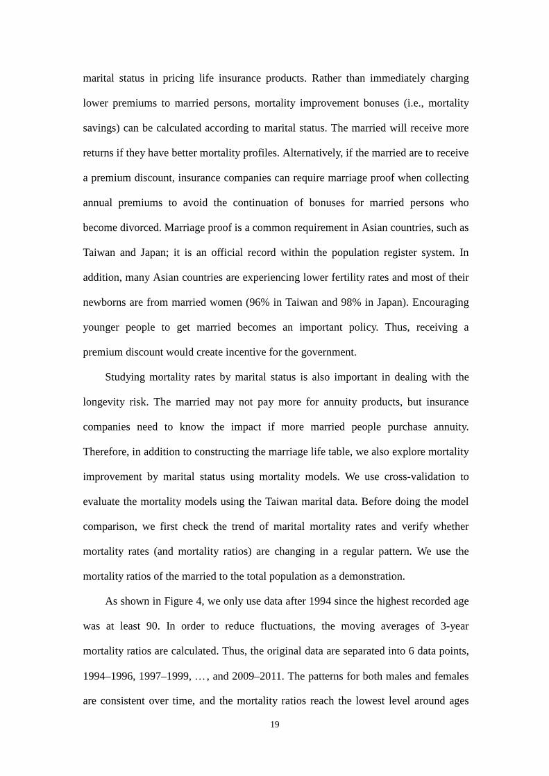
mortality ratios of the married to the total population as a demonstration.
As shown in Figure 4, we only use data after 1994 since the highest recorded age
was at least 90. In order to reduce fluctuations, the moving averages of 3-year
mortality ratios are calculated. Thus, the original data are separated into 6 data points,
1994–1996, 1997–1999, …, and 2009–2011. The patterns for both males and females
are consistent over time, and the mortality ratios reach the lowest level around ages
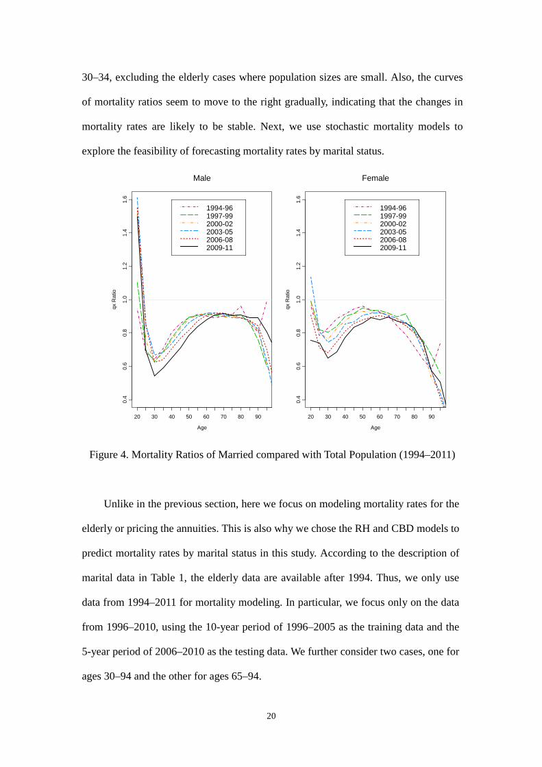
20
30–34, excluding the elderly cases where population sizes are small. Also, the curves
of mortality ratios seem to move to the right gradually, indicating that the changes in
mortality rates are likely to be stable. Next, we use stochastic mortality models to
explore the feasibility of forecasting mortality rates by marital status.
Figure 4. Mortality Ratios of Married compared with Total Population (1994–2011)
Unlike in the previous section, here we focus on modeling mortality rates for the
elderly or pricing the annuities. This is also why we chose the RH and CBD models to
predict mortality rates by marital status in this study. According to the description of
marital data in Table 1, the elderly data are available after 1994. Thus, we only use
data from 1994–2011 for mortality modeling. In particular, we focus only on the data
from 1996–2010, using the 10-year period of 1996–2005 as the training data and the
5-year period of 2006–2010 as the testing data. We further consider two cases, one for
ages 30–94 and the other for ages 65–94.
Male
Age
qx R
atio
20 30 40 50 60 70 80 90
0.4
0.6
0.8
1.0
1.2
1.4
1.6
1994-961997-992000-022003-052006-082009-11
Female
Age
qx R
atio
20 30 40 50 60 70 80 90
0.4
0.6
0.8
1.0
1.2
1.4
1.6
1994-961997-992000-022003-052006-082009-11
21
The four mortality models considered in this study usually apply different
methods to predict future mortality rates. For the LC model, the time series approach
is a popular choice in many studies and we also use it here. The forecast in using the
CBD model is similar to that using the LC model, although computer simulation can
be used. For the RH and RM models, we chose the block bootstrap simulation for
predictions. In particular, the median of 1,000 block bootstrap simulation is treated as
the predicted value.
The model comparison is based on the mean absolute percentage error (MAPE),
or
∑=
×−
=n
i i
ii
Y
YY
nMAPE
1%100
ˆ1 , (10)
where iY and iY
are the observed and predicted values for observation i,
.,,2,1 ni 2= According to Lewis (1982), a prediction with MAPE less than 10% is
treated as highly accurate, and a MAPE greater than 50% is considered inaccurate.
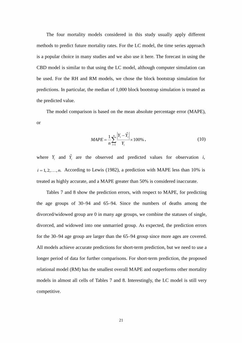
Tables 7 and 8 show the prediction errors, with respect to MAPE, for predicting
the age groups of 30–94 and 65–94. Since the numbers of deaths among the
divorced/widowed group are 0 in many age groups, we combine the statuses of single,
divorced, and widowed into one unmarried group. As expected, the prediction errors
for the 30–94 age group are larger than the 65–94 group since more ages are covered.
All models achieve accurate predictions for short-term prediction, but we need to use a
longer period of data for further comparisons. For short-term prediction, the proposed
relational model (RM) has the smallest overall MAPE and outperforms other mortality
models in almost all cells of Tables 7 and 8. Interestingly, the LC model is still very
competitive.
22
Table 7. Prediction MAPE (%) of Mortality Models (Ages 30–94)
Married Un-married Single
Average Male Female Male Female Male Female
LC 17.3 14.3 6.4 10.0 8.1 15.7 12.3 CBD 8.6 8.7 10.2 15.7 17.7 19.2 12.5 RH 32.7 31.0 5.3 21.0 4.1 23.7 19.7 RM 6.9 5.8 4.4 4.5 7.8 11.6 6.2
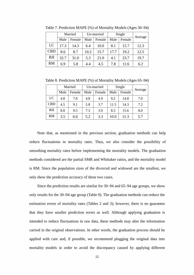
Table 8. Prediction MAPE (%) of Mortality Models (Ages 65–94)
Married Un-married Single
Average Male Female Male Female Male Female
LC 4.8 7.8 4.8 4.9 9.2 14.8 7.0 CBD 4.5 9.1 5.8 3.7 11.5 14.3 7.2 RH 8.8 9.5 7.3 3.9 8.3 15.6 8.0 RM 3.5 6.6 5.2 3.3 10.0 11.3 5.7
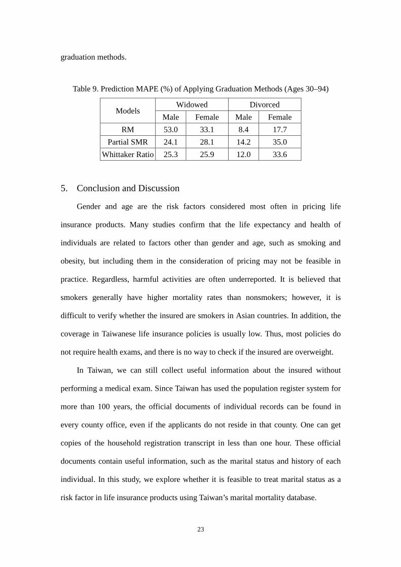
Note that, as mentioned in the previous section, graduation methods can help
reduce fluctuations in mortality rates. Thus, we also consider the possibility of
smoothing mortality rates before implementing the mortality models. The graduation
methods considered are the partial SMR and Whittaker ratios, and the mortality model
is RM. Since the population sizes of the divorced and widowed are the smallest, we
only show the prediction accuracy of these two cases.
Since the prediction results are similar for 30–94 and 65–94 age groups, we show
only results for the 30–94 age group (Table 9). The graduation methods can reduce the
estimation errors of mortality rates (Tables 2 and 3); however, there is no guarantee
that they have smaller prediction errors as well. Although applying graduation is
intended to reduce fluctuations in raw data, these methods may alter the information
carried in the original observations. In other words, the graduation process should be
applied with care and, if possible, we recommend plugging the original data into
mortality models in order to avoid the discrepancy caused by applying different
23
graduation methods.
Table 9. Prediction MAPE (%) of Applying Graduation Methods (Ages 30–94)
Models Widowed Divorced
Male Female Male Female RM 53.0 33.1 8.4 17.7
Partial SMR 24.1 28.1 14.2 35.0 Whittaker Ratio 25.3 25.9 12.0 33.6
5. Conclusion and Discussion
Gender and age are the risk factors considered most often in pricing life
insurance products. Many studies confirm that the life expectancy and health of
individuals are related to factors other than gender and age, such as smoking and
obesity, but including them in the consideration of pricing may not be feasible in
practice. Regardless, harmful activities are often underreported. It is believed that
smokers generally have higher mortality rates than nonsmokers; however, it is
difficult to verify whether the insured are smokers in Asian countries. In addition, the
coverage in Taiwanese life insurance policies is usually low. Thus, most policies do
not require health exams, and there is no way to check if the insured are overweight.
In Taiwan, we can still collect useful information about the insured without
performing a medical exam. Since Taiwan has used the population register system for
more than 100 years, the official documents of individual records can be found in
every county office, even if the applicants do not reside in that county. One can get
copies of the household registration transcript in less than one hour. These official
documents contain useful information, such as the marital status and history of each
individual. In this study, we explore whether it is feasible to treat marital status as a
risk factor in life insurance products using Taiwan’s marital mortality database.
24
The empirical study of Taiwan mortality by marital status confirms that married
people have the lowest mortality rates and highest life expectancy. Comparing with the
unmarried, married males seem to benefit more than married females. For example,
for married and single individuals aged 15, the married male is expected to live about
8 years more than the single male, while the difference for the female is only about 3
years. Moreover, if the premiums of life insurance policies are calculated according to
an individual’s marital status, the discount in premiums for the married over the single
can be as much as 40%. The amount of discount is even larger than discounts offered
to nonsmokers compared with smokers, and to persons of normal weight compared
with obese persons. This confirms that marital status is a feasible factor to be included
in pricing and marketing life insurance products in Taiwan.
In this study of modeling mortality rates by marital status, we find that the
proposed relational model (RM) has the smallest prediction errors, with respect to
MAPE (mean absolute percentage error), and is slightly better than LC, RH, and CBD
models. In addition, the prediction errors of all mortality models are significantly
smaller for the elderly group (65 and over) than those for the younger population (ages
30–64). This might suggest that mortality improvements are not the same for different
ages. However, since we only analyze Taiwan data, and our data period is too short,
we need to collect more data to confirm our findings.
In this study, we also evaluate methods for smoothing mortality rates of small
areas. The proposed methods include information from a large area to reduce
fluctuations in mortality rates in small areas. Treating Taiwan as the large area and
Pen-Hu county as the small area, we find that the partial SMR and Whittaker ratio
have the smallest MSEs. We recommend the Whittaker ratio method. Furthermore, we
find that all graduation methods can help to reduce the MSE of mortality rates,
comparing to ungraduated mortality rates.
25
Note that, although we find mortality rates of the married are lower, we cannot
conclude that being married causes people to live longer. In Taiwan, the proportion of
married people is higher among those with higher income and higher education. We
cannot tell whether marriage, higher income, or higher education causes people to live
longer. On the other hand, the marital data used in this study are at the aggregate level.
It will be more reasonable to use individual data and the idea of multiple decrements
to construct the life table by marital status.
Acknowledgments
The authors are grateful for the insightful comments from two anonymous reviewers.
This research was supported in part by a grant from the Ministry of Science and
Technology in Taiwan, MOST 104-2410-H-156-005.
26
References
Cairns, A.J.G., Blake, D., and Dowd, K. (2006). A Two-Factor Model for Stochastic
Mortality with Parameter Uncertainty: Theory and Calibration. Journal of Risk and
Insurance 73(4), 687-718.
Cairns, A.J.G., Blake, D., Dowd, K., Coughlan, G.D., and Khalaf-Allah, M. (2011)
Bayesian Stochastic Mortality Modelling for Two Populations. Astin Bulletin
41(1), 29-59.
Camarda, C.G. (2012) MortalitySmooth: An R Package for Smoothing Poisson
Counts with P-Splines. Journal of Statistical Software 50(1), 1-24.
Debón, A., Montes, F., Mateu, J., Porcu, E., Bevilacqua, M., (2008) Modelling
Residuals Dependence in Dynamic Life Tables: A Geostatistical Approach.
Computational Statistics and Data Analysis 52, 3128-3147.
Dowd, K., Blake, D., Cairns, A.J.G., Coughlan, G.D., and Khalaf-Allah, M. (2011) A
Gravity Model of Mortality Rates for Two Related Populations. North American
Actuarial Journal 15, 334-356.
eHealth, Inc.
http://www.marketwatch.com/story/smokers-pay-14-higher-health-insurance-premi
ums-than-non-smokers-ehealth-data-shows-2013-01-03.
Gardner, J. and Oswald, A.J. (2004) How is Mortality Affected by Money, Marriage,
and Stress?. Journal of Health Economics 23(6), 1181-1207.
Hu, Y. and Goldman, N. (1990) Mortality Differentials by Marital Status: An
International Comparison. Demography 27(2), 233-250.
Jarner, S.F. and Kryger, E.M. (2011) Modelling Adult Mortality in Small Populations:
The SAINT Model. Astin Bulletin 41(2), 377-418.
Lee, R.D. and Carter, L. (1992) Modeling and Forecasting the Time Series of U.S.
Mortality. Journal of the American Statistical Association 87, 659-675.
Lee, W. (2003) A Partial SMR Approach to Smoothing Age-Specific Rates. Annals of
Epidemiology 13(2), 89-99.
Lewis, E.B. (1982) Control of Body Segment Differentiation in Drosophila by the
Bithorax Gene Complex. In Embryonic Development, Part A: Genetics Aspects.
Edited by M.M. Burger and R. Weber. Alan R. Liss, New York, 269-288.
27
Li, J. S. H., and Hardy, M. R. (2011) Measuring Basis Risk in Longevity Hedges.
North American Actuarial Journal 15(2), 177–200.
Li, N. and Lee, R. (2005) Coherent Mortality Forecasts for a Group of Populations:
An Extension of the Lee-Carter Method. Demography 42(3), 575-594.
Lillard, L.A. and Panis, C.W.A. (1996) Marital Status and Mortality: The Role of
Health. Demography 33(3), 313-327.
London, R.L. (1985) Graduation: The Revision of Estimates. ACTEX Publication.
Martikainen, P., Martelin, T., Nihtilä, E., Majamaa, K., and and Koskinen, S. (2005)
Differences in Mortality by Marital Status in Finland from 1976 to 2000: Analyses
of Changes in Marital-Status Distributions, Socio-Demographic and Household
Composition, and Cause of Death. Population Studies 59(1), 99-115.
Ministry of Economic Affairs, Taiwan. http://twbusiness.nat.gov.tw/old/pdf/sec9.pdf
Ministry of the Interior, Taiwan Government. http://www.moi.gov.tw/stat
Renshaw, A.E. and Haberman, S. (2006) A Cohort-based Extension to the Lee-Carter
Model for Mortality Reduction Factors. Insurance: Mathematics and Economics
38(3), 556-570.
Schwaiger, E. (2005) Preferred Lives-A Concept for Taiwan? Underwriting
Considerations. Munich Re Group.
Trowbridge, C.L. (1994) Mortality Rates by Marital Status. Transactions, Society of
Actuaries, XLVI, 99-122.
United Nations Statistics Division.
http://unstats.un.org/unsd/demographic/sources/popreg/popregmethods.htm
Van den Berg, G.J. and Gupta, S. (2008) Early-life Conditions, Marital Status, and
Mortality. http://www.iza.org/conference_files/SUMS2007/gupta_s3359.pdf
Wang, H.C. and Yue, C.J. (2011) Using Regular Discount Sequence to Model Elderly
Mortality. Journal of Population Studies 43, 40-73. (In Chinese)
Wang, H.C., Jin, S., and Yue, C.J. (2012) A Simulation Study of Small Area Mortality
Projection. Journal of Population Studies 45, 77-110. (In Chinese)
Yue, C.J. (1998) Can Marriage Extend the Life Expectancy – An Empirical Study of
Tawian and U.S.. The Insurance Quarterly, 107, 91-104. (In Chinese)
Yue, C.J. and Huang, H. (2011) A Study of Incidence Experience for Taiwan Life

28
Insurance. Geneva Papers on Risk and Insurance - Issues and Practice 36,
718-733.
Zhou, R., Li, J.S.H., and Tan, K.S. (2013) Pricing Mortality Risk: A Two-Population
Model with Transitory Jump Effects. Journal of Risk and Insurance 80, 733-774.