Marcello Fanti - Home INFN Milanofanti/Particelle4/fanti_Statistics.pdf · Statistical techniques Marcello Fanti Physics Dept. | University of Milano M. Fanti (Physics Dep., UniMi)

Statistical techniques

Marcello Fanti

Physics Dept. — University of Milano

M. Fanti (Physics Dep., UniMi) Statistics 1 / 47

Estimators


Definition of estimator

Assume we run an experiment that performs N independent measurements of a (set of) observable(s) ~x : ~x1,~x2, . . . ,~xNThe measurements ~x1, . . . ,~xN depend on the properties of the system under study (physics process ⊕ apparatus),

which we assume to be described by some parameters ~θ ≡ (θ1, . . . , θp)

From the measurements we want to infer the properties of the system, i.e. the values of the θ1, . . . , θp parameters.

To do this we need to develop some function, or algorithm, to be applied to the measurements:

θk ≡ θk(~x1, . . . ,~xN)

θk this is the estimator of property (or parameter) θk .

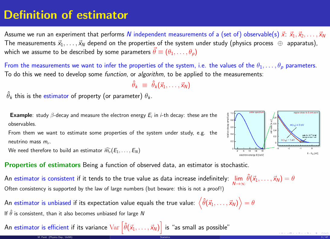
Example: study β-decay and measure the electron energy Ei in i -th decay: these are the

observables.

From them we want to estimate some properties of the system under study, e.g. the

neutrino mass mν.

We need therefore to build an estimator mν(E1, . . . ,EN)

Properties of estimators Being a function of observed data, an estimator is stochastic.

An estimator is consistent if it tends to the true value as data increase indefinitely: limN→∞

θ(~x1, . . . ,~xN) = θ

Often consistency is supported by the law of large numbers (but beware: this is not a proof!)

An estimator is unbiased if its expectation value equals the true value:⟨θ(~x1, . . . ,~xN)

⟩= θ

If θ is consistent, than it also becomes unbiased for large N

An estimator is efficient if its variance Var[θ(~x1, . . . ,~xN)

]is “as small as possible”


Likelihood function


Likelihood function

Measurements are stochastic: the probability that a measurement yields a value in a neighborhood dx of x is

Prob (x ; dx) = f (x ; ~θ) dx which depends on the properties ~θ of the system under exam and of the experimental

apparatus.

The (density of) probability of getting N independent measurements ~x1, . . . ,~xN is

L(~x1, . . . ,~xN ; ~θ

)=

N∏i=1

f (~xi ; ~θ)

if seen as a function of the parameters ~θ, this is called likelihood function

Example: random Poisson counts: Prob (K ) = e−µµK

K !

Repeat the counting N times ⇒ get observables K1, . . . ,KN ⇒ L(µ) =N∏i=1

[e−µ

µKi

Ki !

]— function of parameter µ

Example: decay times: pdf (t) =1

τe−t/τ

Observe N decays ⇒ get observables t1, . . . , tN ⇒ L(τ ) =N∏i=1

[1

τe−ti/τ

]— function of parameter τ

L(~θ) is NOT a pdf of parameters ~θ. Parameters are NOT stochastic — they have precise (although unknown) values.

Integrals like

∫dθL(θ) are meaningless.


Likelihood function and estimators

Assume a model f (~x ; ~θ) ⇒ we know L(~x1, . . . ,~xN ; ~θ

)Assume we defined an estimator θ(~x1, . . . ,~xN). Then, we can compute its properties:

⟨θ⟩

=

∫dx1 · · ·

∫dxN L

(~x1, . . . ,~xN ; ~θ

)θ(~x1, . . . ,~xN) ≡

∫dX L θ⟨

θ2⟩

=

∫dx1 · · ·

∫dxN L

(~x1, . . . ,~xN ; ~θ

) [θ(~x1, . . . ,~xN)

]2

≡∫

dX L θ2

Var[θ]

=⟨θ2⟩−⟨θ⟩2

⇒ Bias and efficiency depend on the likelihood function L, i.e. on the model (≡ system+apparatus)

In principle they could be computed, once the model f (~x ; ~θ) is known, if we are able to work out these integrals!

Alternatively, we could use Monte Carlo technique: sampling a given f (~x ; ~θ) we may generate several times the set of

measurements ~x1, . . . ,~xN and for each time compute ~θ, then see how they are distributed. . .


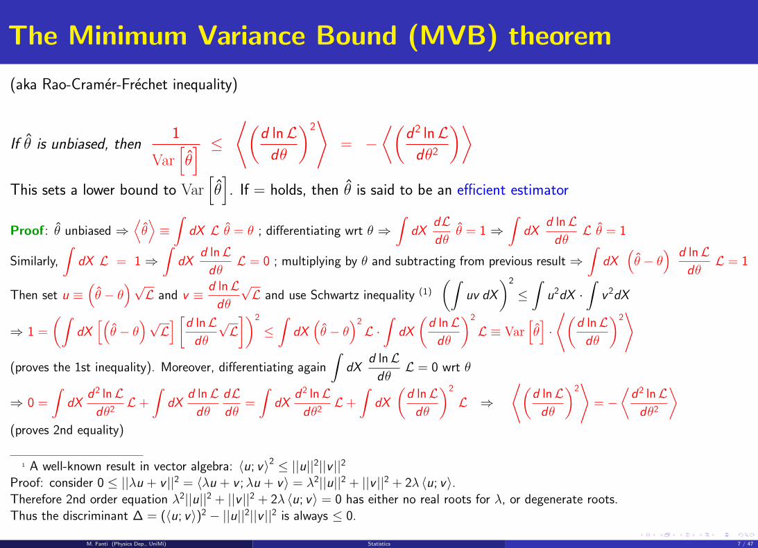
The Minimum Variance Bound (MVB) theorem

(aka Rao-Cramer-Frechet inequality)

If θ is unbiased, then1

Var[θ] ≤ ⟨(

d lnLdθ

)2⟩

= −⟨(

d 2 lnLdθ2

)⟩This sets a lower bound to Var

[θ]

. If = holds, then θ is said to be an efficient estimator

Proof: θ unbiased ⇒⟨θ⟩≡∫

dX L θ = θ ; differentiating wrt θ ⇒∫

dXdLdθ

θ = 1 ⇒∫

dXd lnLdθ

L θ = 1

Similarly,

∫dX L = 1 ⇒

∫dX

d lnLdθ

L = 0 ; multiplying by θ and subtracting from previous result ⇒∫

dX(θ − θ

) d lnLdθ

L = 1

Then set u ≡(θ − θ

)√L and v ≡ d lnL

dθ

√L and use Schwartz inequality (1)

(∫uv dX

)2

≤∫

u2dX ·∫

v 2dX

⇒ 1 =

(∫dX[(θ − θ

)√L] [d lnL

dθ

√L])2

≤∫

dX(θ − θ

)2L ·∫

dX

(d lnLdθ

)2

L ≡ Var[θ]·

⟨(d lnLdθ

)2⟩

(proves the 1st inequality). Moreover, differentiating again

∫dX

d lnLdθ

L = 0 wrt θ

⇒ 0 =

∫dX

d2 lnLdθ2

L+

∫dX

d lnLdθ

dLdθ

=

∫dX

d2 lnLdθ2

L+

∫dX

(d lnLdθ

)2

L ⇒

⟨(d lnLdθ

)2⟩

= −⟨d2 lnLdθ2

⟩(proves 2nd equality)

1 A well-known result in vector algebra: 〈u; v〉2 ≤ ||u||2||v ||2Proof: consider 0 ≤ ||λu + v ||2 = 〈λu + v ;λu + v〉 = λ2||u||2 + ||v ||2 + 2λ 〈u; v〉.Therefore 2nd order equation λ2||u||2 + ||v ||2 + 2λ 〈u; v〉 = 0 has either no real roots for λ, or degenerate roots.Thus the discriminant ∆ = (〈u; v〉)2 − ||u||2||v ||2 is always ≤ 0.


Maximum likelihood estimate


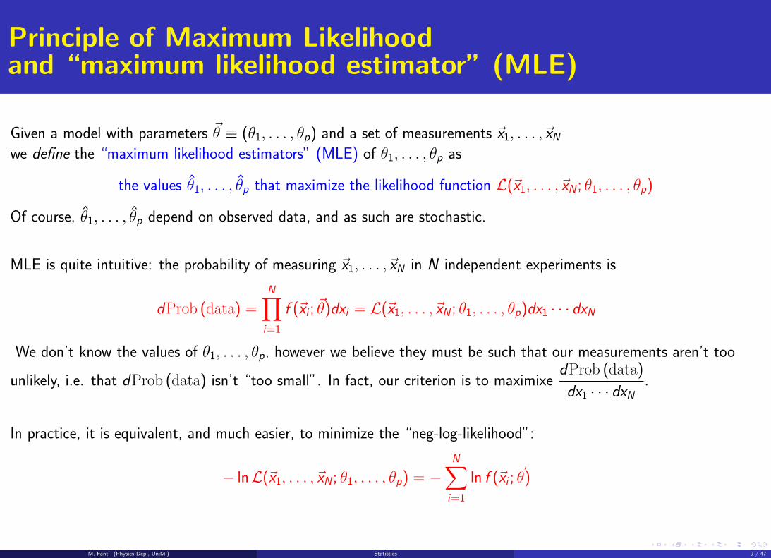
Principle of Maximum Likelihoodand “maximum likelihood estimator” (MLE)

Given a model with parameters ~θ ≡ (θ1, . . . , θp) and a set of measurements ~x1, . . . ,~xNwe define the “maximum likelihood estimators” (MLE) of θ1, . . . , θp as

the values θ1, . . . , θp that maximize the likelihood function L(~x1, . . . ,~xN ; θ1, . . . , θp)

Of course, θ1, . . . , θp depend on observed data, and as such are stochastic.

MLE is quite intuitive: the probability of measuring ~x1, . . . ,~xN in N independent experiments is

dProb (data) =N∏i=1

f (~xi ; ~θ)dxi = L(~x1, . . . ,~xN ; θ1, . . . , θp)dx1 · · · dxN

We don’t know the values of θ1, . . . , θp, however we believe they must be such that our measurements aren’t too

unlikely, i.e. that dProb (data) isn’t “too small”. In fact, our criterion is to maximixedProb (data)

dx1 · · · dxN.

In practice, it is equivalent, and much easier, to minimize the “neg-log-likelihood”:

− lnL(~x1, . . . ,~xN ; θ1, . . . , θp) = −N∑i=1

ln f (~xi ; ~θ)


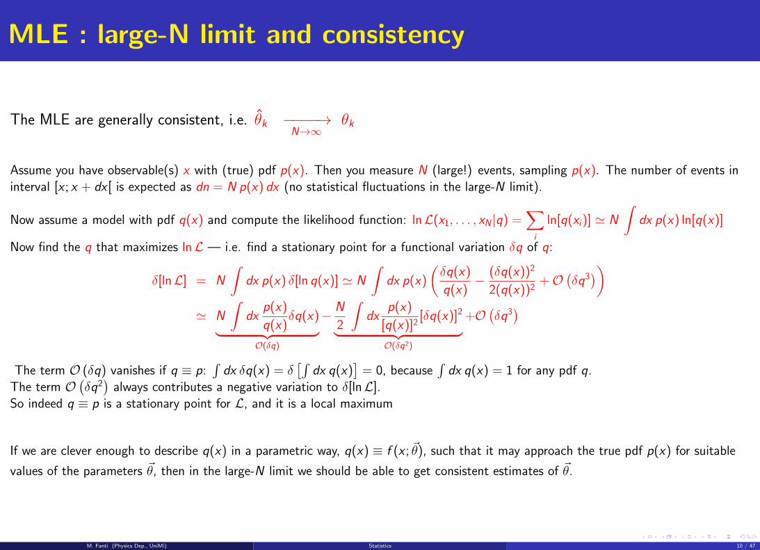
MLE : large-N limit and consistency

The MLE are generally consistent, i.e. θk −−−−→N→∞

θk

Assume you have observable(s) x with (true) pdf p(x). Then you measure N (large!) events, sampling p(x). The number of events ininterval [x ; x + dx [ is expected as dn = N p(x) dx (no statistical fluctuations in the large-N limit).

Now assume a model with pdf q(x) and compute the likelihood function: lnL(x1, . . . , xN |q) =∑i

ln[q(xi)] ' N

∫dx p(x) ln[q(x)]

Now find the q that maximizes lnL — i.e. find a stationary point for a functional variation δq of q:

δ[lnL] = N

∫dx p(x) δ[ln q(x)] ' N

∫dx p(x)

(δq(x)

q(x)− (δq(x))2

2(q(x))2+O

(δq3))

' N

∫dx

p(x)

q(x)δq(x)︸︷︷︸

O(δq)

− N

2

∫dx

p(x)

[q(x)]2[δq(x)]2︸︷︷︸

O(δq2)

+O(δq3)

The term O (δq) vanishes if q ≡ p:∫dx δq(x) = δ

[∫dx q(x)

]= 0, because

∫dx q(x) = 1 for any pdf q.

The term O(δq2)

always contributes a negative variation to δ[lnL].So indeed q ≡ p is a stationary point for L, and it is a local maximum

If we are clever enough to describe q(x) in a parametric way, q(x) ≡ f (x ; ~θ), such that it may approach the true pdf p(x) for suitable

values of the parameters ~θ, then in the large-N limit we should be able to get consistent estimates of ~θ.


MLE : invariance and bias

Assume we have a model with parameters θ1, . . . , θp and compute MLEs for them ⇒ we get θ1, . . . , θp.

Then assume we need to re-parametrize our model with new parameters θ′k = φk(θ1, . . . , θp) and re-compute MLEs

⇒ we get θ′1, . . . , θ′p.

Since both MLE’s give the absolute maximum of L, it must be θ′k = φk(θ1, . . . , θp) :

“the MLEs of the transformed parameters are the transformed of the MLEs of the parameters”

This property is the invariance wrt the choice of the parametrization — a very convenient property!

[e.g. in a neutrino mass measurement, it doesn’t matter whether we choose as parameter mν or m2ν]

As a consequence of invariance, MLEs are generally biased!!!

We cannot have two parametrizations {θk} and {θ′k} whose MLEs are both unbiased.

Unless the transform ~θ → ~θ′ were linear, we know that 〈θ′k〉 6= φk (〈θ1〉 , . . . , 〈θp〉).

Therefore⟨θ′k

⟩=⟨φk(θ1, . . . , θp)

⟩6= φk(

⟨θ⟩1, . . . ,

⟨θ⟩p)

Assume MLEs {θk} are all unbiased ⇒⟨θk

⟩= θk

⇒⟨θ′k

⟩6= φk(θ1, . . . , θp) = θ′k

⇒ {θ′k} are biased!

However, in the large-N limit, MLEs become consistent, limN→∞

θk = θk ,

therefore they also become unbiased: limN→∞

⟨θk

⟩= θk .


MLE in the large-N limit (aka “asymptotic limit”)

In the large-N limit, the MLEs θ ≡ (θ1, . . . , θp) are distributed as a multi-dimensional Gaussian, centered around ~θtrue

and with covariance matrix Cjk ≡ Cov[θj ; θk

]estimated as:

[C−1

]kj

= −[∂2 lnL∂θk ∂θj

]~θ=~θ

⇒ MLEs are consistent (proof on next slide)

The likelihood function takes the form: L(~θ) = Lmax · e−12{∑

j ,k(θj−θj )[C−1]jk(θk−θk)}

The covariance ellipsoids at t-sigma, defined by∑j ,k

(θj − θj)[C−1]jk(θk − θk) = t2 can be drawn along the points ~θ in

the parameters’ space satisfying −2 lnL(~θ) = −2 lnLmax + t2

Other forms of covariance matrix:[C−1

]kj

= −⟨∂2 lnL∂θk ∂θj

⟩=

⟨(∂ lnL∂θj

)(∂ lnL∂θk

)⟩= −N ·

⟨∂2 ln f (~x ; ~θ)

∂θk ∂θj

⟩= N ·

⟨(∂ ln f (~x ; ~θ)

∂θj

)(∂ ln f (~x ; ~θ)

∂θk

)⟩The choice of the form depends on the situation — note that these forms imply integration


MLE in the large-N limit : proof

By construction,

[∂ lnL∂θk

]~θ=~θ

= 0.

From consistency, at large N we expect θk ' θtruek therefore we may expand to 1st order and neglect O((

θ − θtrue)2)

:

0 =

[∂ lnL∂θk

]~θ=~θ

'[∂ lnL∂θk

]~θ=~θtrue

+∑j

(θj − θtruej

) [∂2 lnL∂θk∂θj

]~θ=~θtrue︸︷︷︸

≡ Vkj

⇒ θj − θtruej ' −∑k

[V−1

]jk

∂ lnL∂θk

Now,∂ lnL∂θk

=N∑i=1

∂ ln f (~xi ; ~θ)

∂θkis a sum of N independent stochastic quantities: at large N it is distributed as a Gaussian (central limit

theorem). Therefore,(θj − θtruej

)is also Gaussian-distributed.

Moreover: 1 =

∫dX L ; differentiating wrt θk ⇒ 0 =

∫dX

∂L∂θk

=

∫dX

∂ lnL∂θk

L ⇒⟨∂ lnL∂θk

⟩= 0

⇒(θj − θtruej

)is centered at zero

Differentiating again wrt θj

⇒ 0 =∂

∂θj

∫dX

∂ lnL∂θk

L =

∫dX

∂2 lnL∂θj∂θk

L+

∫dX

∂ lnL∂θk

∂L∂θj

=

∫dX

∂2 lnL∂θj∂θk

L+

∫dX

∂ lnL∂θk

∂ lnL∂θj

L

⇒ −⟨∂2 lnL∂θj∂θk

⟩=

⟨(∂ lnL∂θj

)(∂ lnL∂θk

)⟩Finally, assuming

⟨θk

⟩= θtruek — and neglecting fluctuations induced by data on Vkj ≡

[∂2 lnL∂θk∂θj

]~θ=~θtrue

⇒ Cov[θr ; θs

]=⟨(θr − θtruer

)(θs − θtrues

)⟩=∑k,`

[V−1

]rk

[V−1

]s`

⟨∂ lnL∂θk

∂ lnL∂θ`

⟩= −

∑k ,`

[V−1

]rk

[V−1

]s`

[V]k` = −[V−1

]rs

Invoking again consistency,

[∂2 lnL∂θk∂θj

]~θ=~θtrue

'[∂2 lnL∂θk∂θj

]~θ=~θ

and the proof is done!


MLE : summary

Given a model with parameters ~θ ≡ (θ1, . . . , θp) and observables ~x we can build a pdf for the observables:

pdf (~x) = f (~x ; ~θ)

and a likelihood function L(~θ) =N∏i=1

f (~xi ; ~θ)

We define the maximum likelihood estimators (MLEs) θ as the values of parameters ~θ that maximize L for the given

measurements {~x1, . . . ,~xN} of the observables.

In the large-N limit (aka “asymptotic limit”) the MLEs are consistent, unbiased, and efficient.

Moreover the MLEs are distributed as a p-dimensional Gaussian about the true values ~θtrue:

pdf(θ)

=1

(√

2π)pdet(C)e−1

2

∑j ,k(θj−θtruej )[C−1]jk(θk−θtruek )

whose inverse covariance matrix can be estimated as[C−1

]jk

= −[∂2 lnL∂θj ∂θk

]~θ=~θ

The covariance ellipsoids at t-sigma can be drawn along the ~θ-points in the parameters’ space satisfying

−2 lnL(~θ) = −2 lnL(θ) + t2


Examples:

how to build a likelihood function


Extended likelihood, parameters of interest, and nuisanceparameters

Often an experiment is run for some time, during which it acquires an amount of data not guaranteed a priori: the

number of measurements N is itself random, and Poisson-distributed: Prob (n) = e−µµN

N!.

We therefore introduce the extended likelihood L = e−µµN

N!·

N∏i=1

f(~xi ; ~θ

)and its neg-log:

− lnL = (µ− N lnµ)−N∑i=1

ln f(~xi ; ~θ

)(we omitted ln N! as it does not depend on parameters ~θ, ~ν, hence it plays no role in the minimization)

The PDF of the observables ~x often depends on several parameters, that we classify in two groups:

parameters of interest (POIs): those we want to measure from our observation

nuisance parameters (NPs): those we are not interested in, yet cannot be neglected in a complete description of

the model

We’ll write the PDF of the observables as f(~x ; ~θ, ~ν

)to put in evidence the separation between POIs ~θ and NPs ~ν.

Remember: a parametric model must be flexible enough to adapt to our data, otherwise all properties of MLE are

spoiled — even consistency! This means that f(~x ; ~θ, ~ν

), for some values of ~θ, ~ν, should be capable to approach the

“true PDF” f true (~x) as close as needed. This often implies the introduction of many NPs.


Example: likelihood function for a lifetime measurement

Example 1: we observe N decays occurring at times t1, . . . , tN and we want to estimate the average lifetime τ .

The PDF for ti is f (ti) =e−ti/τ

τ, the likelihood function is: L =

∏i

e−ti/τ

τ⇒ − lnL =

∑i

(tiτ

+ ln τ)

Imposing 0 =∂(− lnL)

∂τ= −

∑i

tiτ 2

+N

τ⇒ τ =

1

N

∑i

ti — the average of measured ti ’s, as expected. . .

Example 2: the number N of events is also random — e.g. in case the experiment runs for a pre-fixed time:

Prob (N) = e−µµN

N!⇒ − lnL =

∑i

(tiτ

+ ln τ)

+ µ− N lnµ + ln N! (“extended likelihood function”)

⇒ τ does not change, and imposing∂(− lnL)

∂µ= 0 we get µ = N . Moreover

∂2(lnL)

∂µ ∂τ= 0 ⇒ Cov [µ; τ ] = 0

Example 3: the detector can measure only decay times in a given interval: tMIN < ti < tMAX , therefore

f (ti) =e−ti/τ

τ

(e−tMIN/τ − e−tMAX /τ

)and − lnL =

∑i

[tiτ

+ ln τ − ln(e−tMIN/τ − e−tMAX /τ)]

+ µ− N lnµ + ln N!

⇒ get τ , µ through numeric minimization — factor(e−tMIN/τ − e−tMAX/τ

)comes from pdf normalization: 1 =

∫ tMAX

tMIN

dt f (t)

What if tMIN , tMAX are also unknown? We may extract MLEs τ , µ, tMIN , tMAX from data, with their covariance

matrix and possibly a hyper-covariance-contour in a 4-D parameter space, but is this what we really want?

We rather would like to estimate τ and its uncertainty, regardless of the actual values of µ, tMIN , tMAX .

In this case, µ, tMIN , tMAX are “nuisance parameters” – whereas τ is the “parameter of interest” (POI)


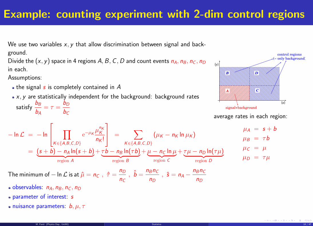
Example: counting experiment with 2-dim control regions

We use two variables x , y that allow discrimination between signal and back-

ground.

Divide the (x , y) space in 4 regions A,B ,C ,D and count events nA, nB , nC , nDin each.

Assumptions:

the signal s is completely contained in A

x , y are statistically independent for the background: background rates

satisfybBbA

= τ =bDbC

− lnL = − ln

∏K∈{A,B ,C ,D}

e−µKµnKK

nK !

=∑

K∈{A,B ,C ,D}

(µK − nK lnµK )

= (s + b)− nA ln(s + b)︸︷︷︸region A

+ τb − nB ln(τb)︸︷︷︸region B

+µ− nC lnµ︸︷︷︸region C

+ τµ− nD ln(τµ)︸︷︷︸region D

The minimum of− lnL is at µ = nC , τ =nDnC

, b =nBnC

nD, s = nA −

nBnCnD

{x}

{y}

control regions(~ only background)

signal+background

A

B

C

D

average rates in each region:

µA = s + b

µB = τb

µC = µ

µD = τµ

observables: nA, nB , nC , nD

parameter of interest: s

nuisance parameters: b, µ, τ


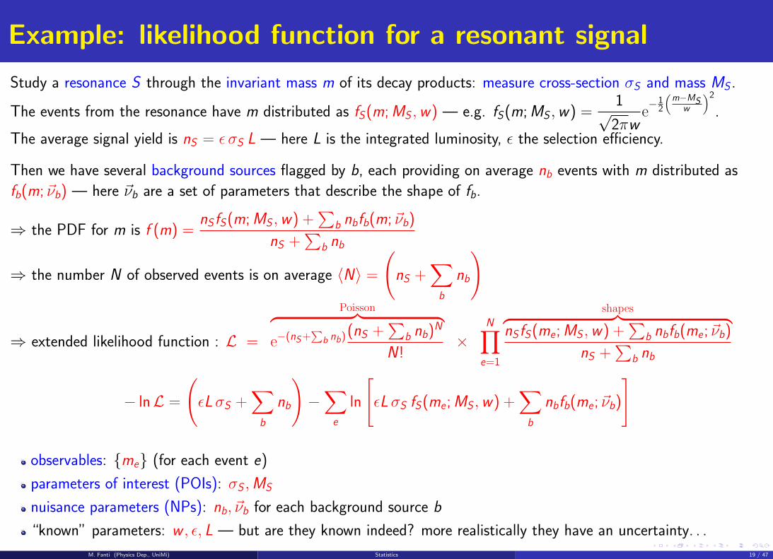
Example: likelihood function for a resonant signal

Study a resonance S through the invariant mass m of its decay products: measure cross-section σS and mass MS .

The events from the resonance have m distributed as fS(m; MS ,w) — e.g. fS(m; MS ,w) =1√

2πwe−1

2

(m−MS

w

)2.

The average signal yield is nS = ε σS L — here L is the integrated luminosity, ε the selection efficiency.

Then we have several background sources flagged by b, each providing on average nb events with m distributed as

fb(m;~νb) — here ~νb are a set of parameters that describe the shape of fb.

⇒ the PDF for m is f (m) =nS fS(m; MS ,w) +

∑b nbfb(m;~νb)

nS +∑

b nb

⇒ the number N of observed events is on average 〈N〉 =

(nS +

∑b

nb

)

⇒ extended likelihood function : L =

Poisson︷︸︸︷e−(nS+

∑b nb) (nS +

∑b nb)N

N!×

N∏e=1

shapes︷︸︸︷nS fS(me; MS ,w) +

∑b nbfb(me;~νb)

nS +∑

b nb

− lnL =

(εLσS +

∑b

nb

)−∑e

ln

[εLσS fS(me; MS ,w) +

∑b

nbfb(me;~νb)

]

observables: {me} (for each event e)

parameters of interest (POIs): σS ,MS

nuisance parameters (NPs): nb, ~νb for each background source b

“known” parameters: w , ε, L — but are they known indeed? more realistically they have an uncertainty. . .


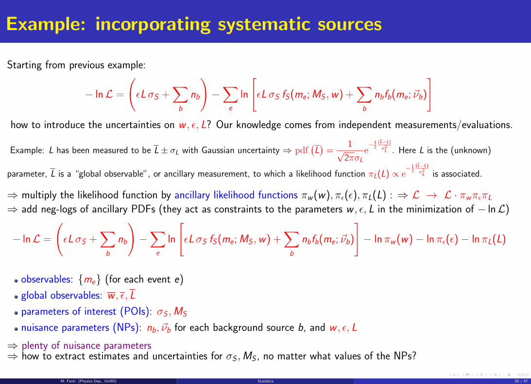
Example: incorporating systematic sources

Starting from previous example:

− lnL =

(εLσS +

∑b

nb

)−∑e

ln


∑b

nbfb(me;~νb)

]how to introduce the uncertainties on w , ε, L? Our knowledge comes from independent measurements/evaluations.

Example: L has been measured to be L± σL with Gaussian uncertainty ⇒ pdf(L)

=1√

2πσLe− 1

2(L−L)

σ2L . Here L is the (unknown)

parameter, L is a “global observable”, or ancillary measurement, to which a likelihood function πL(L) ∝ e− 1

2(L−L)

σ2L is associated.

⇒ multiply the likelihood function by ancillary likelihood functions πw(w), πε(ε), πL(L) : ⇒ L → L · πwπεπL⇒ add neg-logs of ancillary PDFs (they act as constraints to the parameters w , ε, L in the minimization of − lnL)

− lnL =

(εLσS +

∑b

nb

)−∑e

ln


∑b

nbfb(me;~νb)

]− ln πw(w)− ln πε(ε)− lnπL(L)

observables: {me} (for each event e)

global observables: w , ε, L

parameters of interest (POIs): σS ,MS

nuisance parameters (NPs): nb, ~νb for each background source b, and w , ε, L

⇒ plenty of nuisance parameters⇒ how to extract estimates and uncertainties for σS ,MS , no matter what values of the NPs?


Frequentist statistics


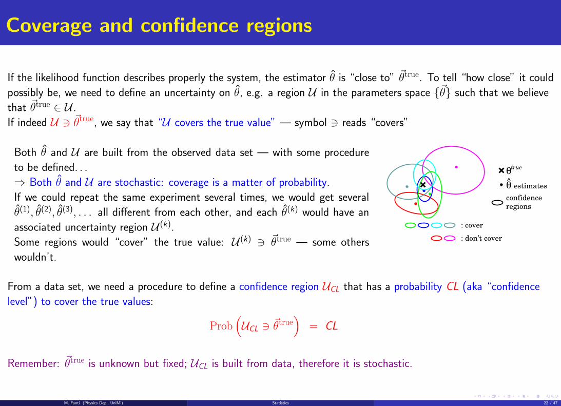
Coverage and confidence regions

If the likelihood function describes properly the system, the estimator θ is “close to” ~θtrue. To tell “how close” it could

possibly be, we need to define an uncertainty on θ, e.g. a region U in the parameters space {~θ} such that we believe

that ~θtrue ∈ U .

If indeed U 3 ~θtrue, we say that “U covers the true value” — symbol 3 reads “covers”

Both θ and U are built from the observed data set — with some procedure

to be defined. . .

⇒ Both θ and U are stochastic: coverage is a matter of probability.

If we could repeat the same experiment several times, we would get several

θ(1), θ(2), θ(3), . . . all different from each other, and each θ(k) would have an

associated uncertainty region U (k).

Some regions would “cover” the true value: U (k) 3 ~θtrue — some others

wouldn’t.

θtrue

θ estimates^

: cover

: don’t cover

confidenceregions

From a data set, we need a procedure to define a confidence region UCL that has a probability CL (aka “confidence

level”) to cover the true values:

Prob(UCL 3 ~θtrue

)= CL

Remember: ~θtrue is unknown but fixed; UCL is built from data, therefore it is stochastic.


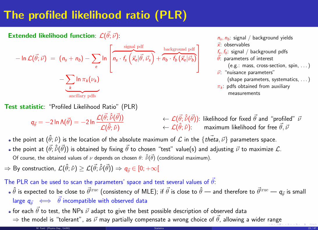
The profiled likelihood ratio (PLR)

Extended likelihood function: L(~θ;~ν):

− lnL(~θ;~ν) = (ns + nb)−∑e

ln

signal pdf︷︸︸︷

ns · fs(~xe|~θ, ~νs

)+

background pdf︷︸︸︷nb · fb (~xe|~νb)

−∑k

ln πk(νk)︸︷︷︸ancillary pdfs

ns , nb: signal / background yields~x : observablesfs , fb: signal / background pdfs~θ: parameters of interest

(e.g.: mass, cross-section, spin, . . . )~ν: “nuisance parameters”

(shape parameters, systematics, . . . )πk : pdfs obtained from auxiliary

measurements

Test statistic: “Profiled Likelihood Ratio” (PLR)

q~θ = −2 ln Λ(~θ) = −2 lnL(~θ; ˆν(~θ))

L(θ; ν)

← L(~θ; ˆν(~θ)): likelihood for fixed ~θ and “profiled” ~ν

← L(θ; ν): maximum likelihood for free ~θ, ~ν

the point at (θ; ν) is the location of the absolute maximum of L in the { ~theta, ~ν} parameters space.

the point at (~θ; ˆν(~θ)) is obtained by fixing ~θ to chosen “test” value(s) and adjusting ~ν to maximize L.

Of course, the obtained values of ν depends on chosen θ: ˆν(~θ) (conditional maximum).

⇒ By construction, L(θ; ν) ≥ L(~θ; ˆν(~θ)) ⇒ q~θ ∈ [0; +∞[

The PLR can be used to scan the parameters’ space and test several values of ~θ:

θ is expected to be close to ~θtrue (consistency of MLE); if ~θ is close to θ — and therefore to ~θtrue — q~θ is small

large q~θ ⇐⇒ ~θ incompatible with observed data

for each ~θ to test, the NPs ~ν adapt to give the best possible description of observed data

⇒ the model is “tolerant”, as ~ν may partially compensate a wrong choice of ~θ, allowing a wider rangeM. Fanti (Physics Dep., UniMi) Statistics 23 / 47

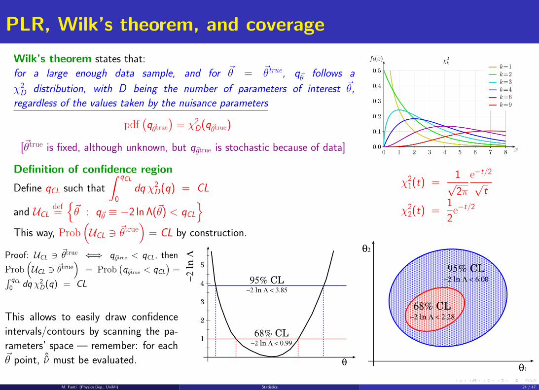
PLR, Wilk’s theorem, and coverage

Wilk’s theorem states that:

for a large enough data sample, and for ~θ = ~θtrue, q~θ follows a

χ2D distribution, with D being the number of parameters of interest ~θ,

regardless of the values taken by the nuisance parameters

pdf(

q~θtrue)

= χ2D(q~θtrue)

[~θtrue is fixed, although unknown, but q~θtrue is stochastic because of data]

Definition of confidence region

Define qCL such that

∫ qCL

0

dq χ2D(q) = CL

and UCLdef={~θ : q~θ ≡ −2 ln Λ(~θ) < qCL

}This way, Prob

(UCL 3 ~θtrue

)= CL by construction.

χ21(t) =

1√2π

e−t/2

√t

χ22(t) =

1

2e−t/2

Proof: UCL 3 ~θtrue ⇐⇒ q~θtrue < qCL, then

Prob(UCL 3 ~θtrue

)= Prob

(q~θtrue < qCL

)=∫ qCL

0 dq χ2D(q) = CL

This allows to easily draw confidence

intervals/contours by scanning the pa-

rameters’ space — remember: for each~θ point, ˆν must be evaluated. θ

68% CL−2 ln Λ < 0.99

95% CL−2 ln Λ < 3.85

−2

ln

Λ

1

2

3

4

5

θ1

θ2

68% CL−2 ln Λ < 2.28

95% CL−2 ln Λ < 6.00


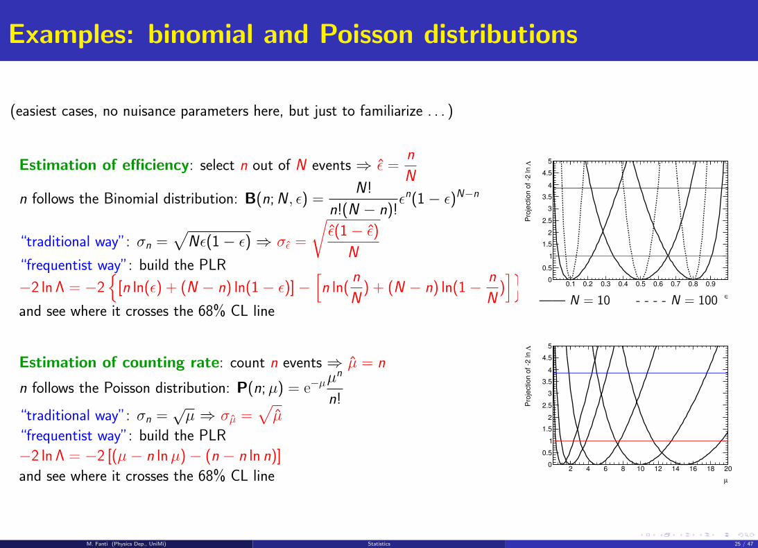
Examples: binomial and Poisson distributions

(easiest cases, no nuisance parameters here, but just to familiarize . . . )

Estimation of efficiency: select n out of N events ⇒ ε =n

N

n follows the Binomial distribution: B(n; N , ε) =N!

n!(N − n)!εn(1− ε)N−n

“traditional way”: σn =√

Nε(1− ε) ⇒ σε =

√ε(1− ε)

N“frequentist way”: build the PLR

−2 ln Λ = −2{

[n ln(ε) + (N − n) ln(1− ε)]−[

n ln(n

N) + (N − n) ln(1− n

N)]}

and see where it crosses the 68% CL line∈

0.1 0.2 0.3 0.4 0.5 0.6 0.7 0.8 0.9

ΛP

roje

ction o

f 2

ln

0

0.5

1

1.5

2

2.5

3

3.5

4

4.5

5

—— N = 10 - - - - N = 100

Estimation of counting rate: count n events ⇒ µ = n

n follows the Poisson distribution: P(n;µ) = e−µµn

n!“traditional way”: σn =

√µ ⇒ σµ =

√µ

“frequentist way”: build the PLR

−2 ln Λ = −2 [(µ− n lnµ)− (n − n ln n)]

and see where it crosses the 68% CL line µ

2 4 6 8 10 12 14 16 18 20

ΛP

roje

ction o

f 2

ln

0

0.5

1

1.5

2

2.5

3

3.5

4

4.5

5


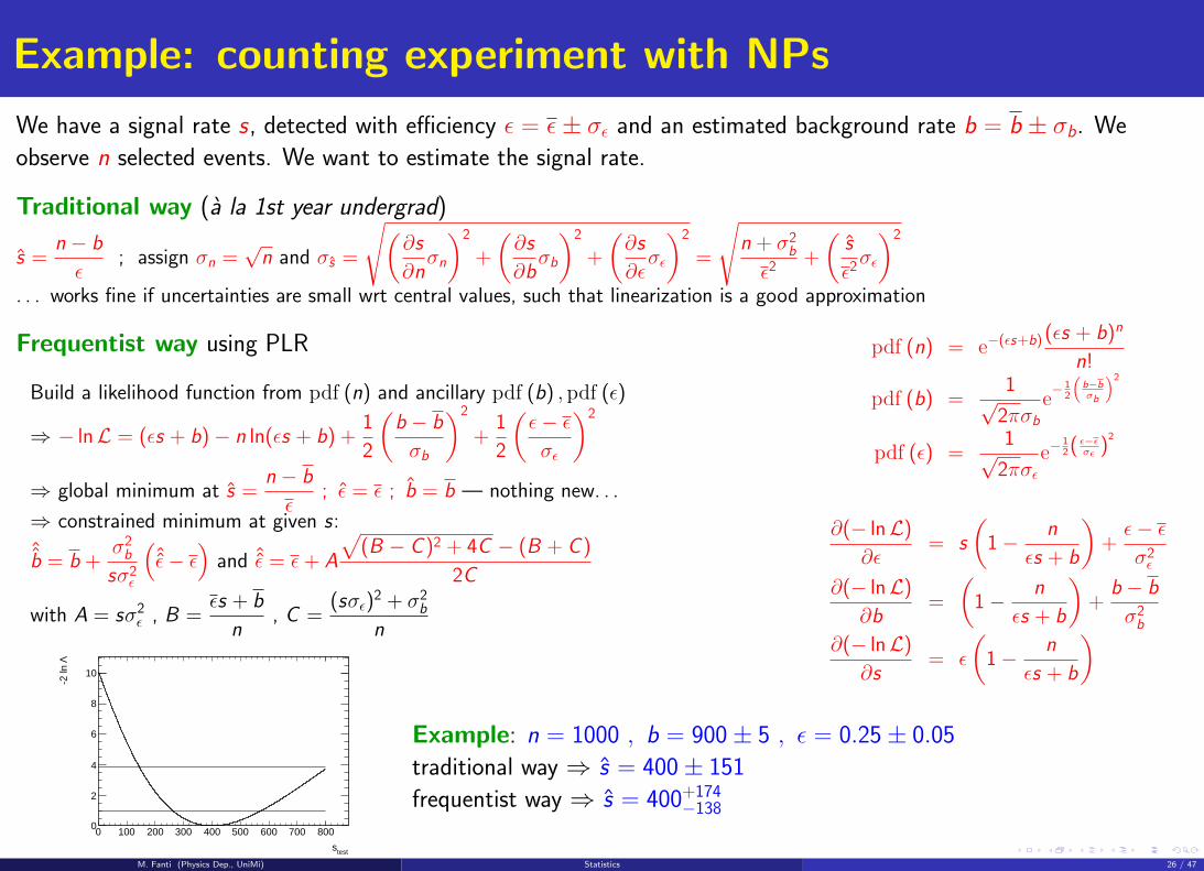
Example: counting experiment with NPs

We have a signal rate s, detected with efficiency ε = ε± σε and an estimated background rate b = b ± σb. We

observe n selected events. We want to estimate the signal rate.

Traditional way (a la 1st year undergrad)

s =n − b

ε; assign σn =

√n and σs =

√(∂s

∂nσn

)2

+

(∂s

∂bσb

)2

+

(∂s

∂εσε

)2

=

√n + σ2bε2

+

(s

ε2σε

)2

. . . works fine if uncertainties are small wrt central values, such that linearization is a good approximation

Frequentist way using PLR

Build a likelihood function from pdf (n) and ancillary pdf (b) , pdf (ε)

⇒ − lnL = (εs + b)− n ln(εs + b) +1

2

(b − b

σb

)2

+1

2

(ε− εσε

)2

⇒ global minimum at s =n − b

ε; ε = ε ; b = b — nothing new. . .

⇒ constrained minimum at given s:

ˆb = b +σ2bsσ2ε

(ˆε− ε

)and ˆε = ε + A

√(B − C )2 + 4C − (B + C )

2C

with A = sσ2ε , B =εs + b

n, C =

(sσε)2 + σ2bn

pdf (n) = e−(εs+b) (εs + b)n

n!

pdf (b) =1√

2πσbe− 1

2

(b−bσb

)2

pdf (ε) =1√

2πσεe−

12(

ε−εσε )

2

∂(− lnL)

∂ε= s

(1− n

εs + b

)+ε− εσ2ε

∂(− lnL)

∂b=

(1− n

εs + b

)+

b − b

σ2b∂(− lnL)

∂s= ε

(1− n

εs + b

)

tests

0 100 200 300 400 500 600 700 800

Λ-2

ln

0

2

4

6

8

10

Example: n = 1000 , b = 900± 5 , ε = 0.25± 0.05

traditional way ⇒ s = 400± 151

frequentist way ⇒ s = 400+174−138


Testing the coverage

The Wilk’s theorem and the PLR method are proved valid for large N (asymptotic limit).

They often work in practice for not-so-high N , but it’s not guaranteed: one needs to test it with “Monte Carlo toys”

Find a PDF for observables, f (~x ; ~θ, ~ν) that describes the data in a good way, and fit it to data.

⇒ get MLEs θdata, νdata from data

Now assume these are the “true values” and use them to generate several pseudo-experiments:

generate N measurements ~x toy1 , . . . ,~x toy

N of the observables, by sampling f (~x ; θdata, νdata)

(N may be fixed to a value, or Poisson-distributed around the observed Ndata)

evaluate MLEs θtoy, νtoy from ~x toy1 , . . . ,~x toy

N

compute qtoy

θdata— i.e. use test value θ = θdata but absolute maximum at θtoy, νtoy

evaluate the confidence region U toyCL as described

check whether θdata ∈ U toyCL (“coverage”) — this actually means: check if qtoy

θdata< qCL

Repeating several times the above procedure several times, we obtain a distribution of qtoy

θdata

⇒ does it follow a χ2D law?

We can also compute the fraction of times fcov in which the confidence region “covers” the true values:

if fcov ' CL then the coverage is well calibrated;

if fcov < CL we have under-coverage;

if fcov > CL we have over-coverage.


Hypothesis testing


Few concepts

Typically we want to see if observed data favour (or not) a given hypothesis

Example: does the Higgs boson exist? ⇒ collect a big lot of experimental data, and try to understand from them if

the Higgs boson were produced. . . HOW???

Data are stochastic:

quantum mechanics is not deterministic: the products of an interaction, and their kinematics distributions, obey

probabilistic rules;

moreover we have all sort of experimental effects, particle-material interactions, detector responses, etc)

⇒ need a precise formulation of the problem, based on unambiguous statistical concepts (2)

On the contrary, the hypothesis is not stochastic, it is either true or false! Our inference will always tell how a given

hypothesis is likely to produce the data we actually observe. It will never tell us “what is the probability that an

hypothesis be true”. This is called “frequentist approach” (3)

2 the difference between probability theory and statistics: P.T. allows to evaluate the probability of obtaining a givenexperimental result, when a specific model is assumed; statistics try to infer the model(s) that better describe a givenexperimental result.

3 As an alternative, the “Bayesian approach” tries to address exactly the probability of the hypothesis, based on theBayes inversion formula

Prob (theory|data) =Prob (data|theory)Prob (theory)∑k Prob (data|theoryk)Prob (theoryk)

The formula itself is true, however the “a priori” theory probability Prob (theory) is generally unknown, and the resultwill depend on how it is chosen


Simple and composite hypothesis, likelihood function

For a given hypothesis H, we assume we are able to evaluate the probability (density) of getting the observed data, ~x

A simple hypothesis does not involve parameters ⇒ we need to consider pdf (~x |H)

(e.g. H ≡ the Higgs boson does not exist)

A composite hypothesis contains one or more parameters, ~θ ≡ (θ1, . . . , θp) ⇒ we need to consider a

pdf(~x |H(~θ)

)= L(~x , ~θ)

(e.g. H ≡ the Higgs boson exists, has mass mH , is produced with cross-section σH)

In composite models, L(~x , ~θ) can be regarded as a function of the parameters ~θ: in this case it is called likelihood

function

It is NOT the probability density for the parameters ~θ!: integrals such as∫

dpθL(~x , ~θ) have no meaning

Some example of composite hypotheses

We count a number n of events (selected in some way) and our hypothesis is that they are Poisson-distributed with average µ. Thelikelihood function is L(n, µ) = e−µµn/n!.

We measure a decay time t whose probability density is exponential, with average τ . Now the likelihood function is

L(t, τ) = 1/τ · e−t/τ .

In composite models, the parameters may be classified as “parameters of interest” (POI), those we want to

test/measure or “nuisance parameters”.

Example: we are searching for a signal of new physics, produced with a rate s, but our sample is contaminated by a background, withrate b ⇒ The probability of observing n events is Prob (n|s, b) = e−(s+b)(s + b)n/n!

Both s, b play a role, but we want to test whether a signal exists with a rate s, we don’t care about b ⇒ b is a nuisance parameter.


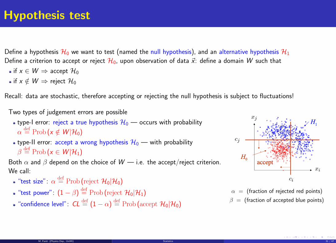
Hypothesis test

Define a hypothesis H0 we want to test (named the null hypothesis), and an alternative hypothesis H1

Define a criterion to accept or reject H0, upon observation of data ~x : define a domain W such that

if x ∈ W ⇒ accept H0

if x /∈ W ⇒ reject H0

Recall: data are stochastic, therefore accepting or rejecting the null hypothesis is subject to fluctuations!

Two types of judgement errors are possible

type-I error: reject a true hypothesis H0 — occurs with probability

αdef= Prob (x /∈ W |H0)

type-II error: accept a wrong hypothesis H0 — with probability

βdef= Prob (x ∈ W |H1)

Both α and β depend on the choice of W — i.e. the accept/reject criterion.

We call:

“test size”: αdef= Prob (reject H0|H0)

“test power”: (1− β)def= Prob (reject H0|H1)

“confidence level”: CLdef= (1− α)

def= Prob (accept H0|H0)

α = (fraction of rejected red points)

β = (fraction of accepted blue points)


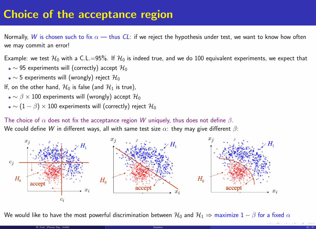
Choice of the acceptance region

Normally, W is chosen such to fix α — thus CL: if we reject the hypothesis under test, we want to know how often

we may commit an error!

Example: we test H0 with a C.L.=95%. If H0 is indeed true, and we do 100 equivalent experiments, we expect that

∼ 95 experiments will (correctly) accept H0

∼ 5 experiments will (wrongly) reject H0

If, on the other hand, H0 is false (and H1 is true),

∼ β × 100 experiments will (wrongly) accept H0

∼ (1− β)× 100 experiments will (correctly) reject H0

The choice of α does not fix the acceptance region W uniquely, thus does not define β.

We could define W in different ways, all with same test size α: they may give different β:

We would like to have the most powerful discrimination between H0 and H1 ⇒ maximize 1− β for a fixed α


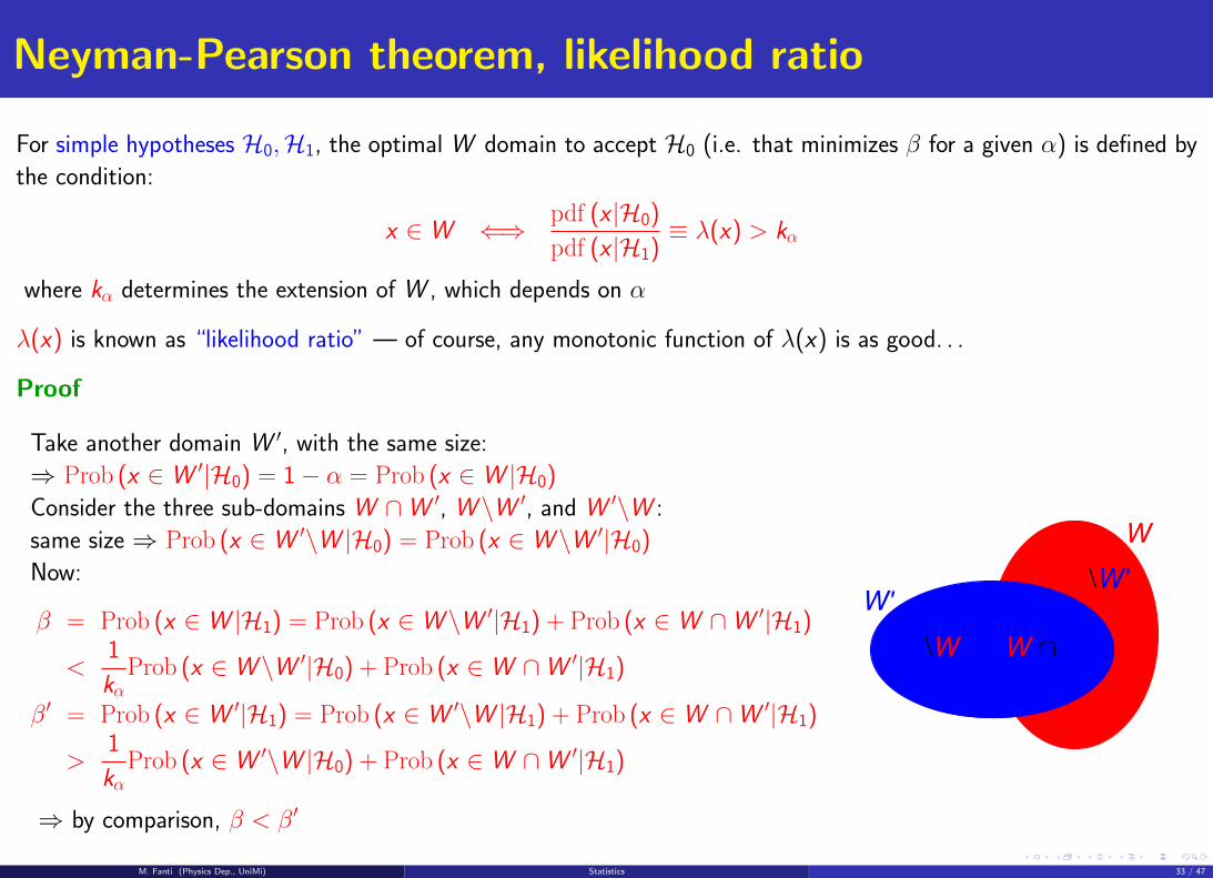
Neyman-Pearson theorem, likelihood ratio

For simple hypotheses H0,H1, the optimal W domain to accept H0 (i.e. that minimizes β for a given α) is defined by

the condition:

x ∈ W ⇐⇒ pdf (x |H0)

pdf (x |H1)≡ λ(x) > kα

where kα determines the extension of W , which depends on α

λ(x) is known as “likelihood ratio” — of course, any monotonic function of λ(x) is as good. . .

Proof

Take another domain W ′, with the same size:

⇒ Prob (x ∈ W ′|H0) = 1− α = Prob (x ∈ W |H0)

Consider the three sub-domains W ∩W ′, W \W ′, and W ′\W :

same size ⇒ Prob (x ∈ W ′\W |H0) = Prob (x ∈ W \W ′|H0)

Now:

β = Prob (x ∈ W |H1) = Prob (x ∈ W \W ′|H1) + Prob (x ∈ W ∩W ′|H1)

<1

kαProb (x ∈ W \W ′|H0) + Prob (x ∈ W ∩W ′|H1)

β′ = Prob (x ∈ W ′|H1) = Prob (x ∈ W ′\W |H1) + Prob (x ∈ W ∩W ′|H1)

>1

kαProb (x ∈ W ′\W |H0) + Prob (x ∈ W ∩W ′|H1)

⇒ by comparison, β < β′

W

W'W \W'

W' \W W ∩W'


Example: a simple counting experiment

Consider the null hypothesis: H0 ≡ “there is a new physics signal, with rate s , on top of a background with rate b”

and the alternative hypothesis: H1 ≡ “there is only a background with rate b”

Prob (n|H0) = e−(s+b) (s+b)n

n! ; Prob (n|H1) = e−b bn

n!

λ(n) = e−s(

1 + sb

)nλ is a monotonically increasing function of n ⇒ we can choose directly n: accept null (signal) hypothesis if n > nα

The boundary nα is fixed by the choice of α: e−(s+b)

[∑n≤nα

(s + b)n/n!

]≤ α

. . . easy, intuitive . . . much too simple!

Even in a counting experiment, s and b are never absolutely well specified.

The background (in this case, Standard Model processes) may be well known from previous measurements, but will

always carry systematics uncertainties, and its rate b depends anyway on this analysis (detector, acceptance,

selection. . . )

The signal rate (being “new physics”) is known only from the theory model, therefore its rate s is precise up to the

achieved evaluation level: it may suffer by neglecting higher-order diagrams, or by poor knowledge of

phenomenological inputs (e.g. parton density functions). Moreover, its observable rate also depends on the

detection and selection efficiency: s = ε · sth

Even in this simple case, the model contains parameters. b and ε are examples on nuisance parameters, sth is the POI

(to be extracted and compared with theoretical predictions)


Test statistic, p-value

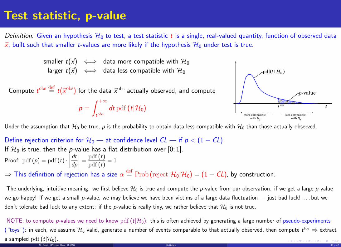
Definition: Given an hypothesis H0 to test, a test statistic t is a single, real-valued quantity, function of observed data

~x , built such that smaller t-values are more likely if the hypothesis H0 under test is true.

smaller t(~x) ⇐⇒ data more compatible with H0

larger t(~x) ⇐⇒ data less compatible with H0

Compute tobsdef= t(~xobs) for the data ~xobs actually observed, and compute

p =

∫ +∞

tobsdt pdf (t|H0) tt

obs

p-value

pdf(t|H )0

more compatiblewith H

0

less compatiblewith H

0

Under the assumption that H0 be true, p is the probability to obtain data less compatible with H0 than those actually observed.

Define rejection criterion for H0 — at confidence level CL — if p < (1− CL)

If H0 is true, then the p-value has a flat distribution over [0; 1].

Proof: pdf (p) = pdf (t) ·∣∣∣∣dtdp∣∣∣∣ =

pdf (t)

pdf (t)= 1

⇒ This definition of rejection has a size αdef= Prob (reject H0|H0) = (1− CL), by construction.

The underlying, intuitive meaning: we first believe H0 is true and compute the p-value from our observation. if we get a large p-value

we go happy! if we get a small p-value, we may believe we have been victims of a large data fluctuation — just bad luck! . . . but we

don’t tolerate bad luck to any extent: if the p-value is really tiny, we rather believe that H0 is not true.

NOTE: to compute p-values we need to know pdf (t|H0): this is often achieved by generating a large number of pseudo-experiments

(“toys”): in each, we assume H0 valid, generate a number of events comparable to that actually observed, then compute ttoy ⇒ extract

a sampled pdf (t|H0).M. Fanti (Physics Dep., UniMi) Statistics 35 / 47

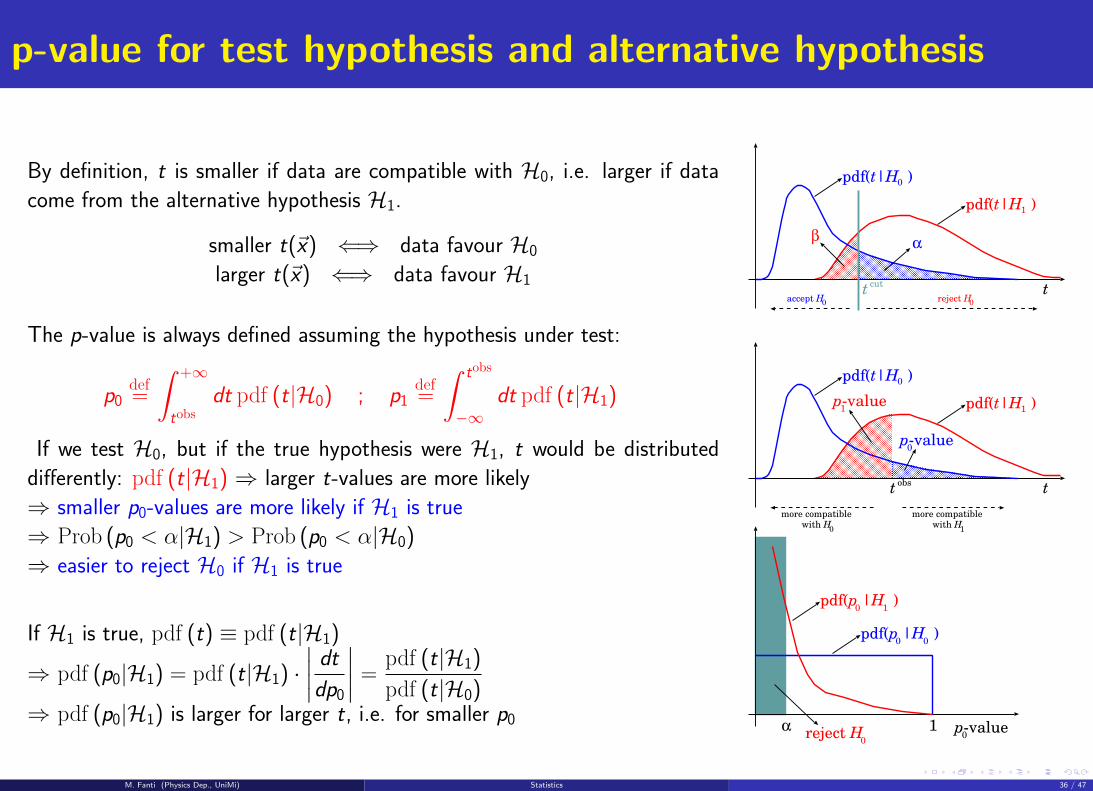
p-value for test hypothesis and alternative hypothesis

By definition, t is smaller if data are compatible with H0, i.e. larger if data

come from the alternative hypothesis H1.

smaller t(~x) ⇐⇒ data favour H0

larger t(~x) ⇐⇒ data favour H1

The p-value is always defined assuming the hypothesis under test:

p0def=

∫ +∞

tobsdt pdf (t|H0) ; p1

def=

∫ tobs

−∞dt pdf (t|H1)

If we test H0, but if the true hypothesis were H1, t would be distributed

differently: pdf (t|H1) ⇒ larger t-values are more likely

⇒ smaller p0-values are more likely if H1 is true

⇒ Prob (p0 < α|H1) > Prob (p0 < α|H0)

⇒ easier to reject H0 if H1 is true

If H1 is true, pdf (t) ≡ pdf (t|H1)

⇒ pdf (p0|H1) = pdf (t|H1) ·∣∣∣∣ dt

dp0

∣∣∣∣ =pdf (t|H1)

pdf (t|H0)⇒ pdf (p0|H1) is larger for larger t, i.e. for smaller p0

ttobs

pdf(t|H )0


0


1

pdf(t|H )1

p-value0

p-value0

pdf(p |H )00

pdf(p |H )10

1αreject H

0

ttcut

pdf(t|H )0

pdf(t|H )1

α

reject H0

accept H0

β

p-value1


Examples of test statistics

A perfect example: the likelihood ratio

The likelihood ratio λ(~x) =pdf (~x |H0)

pdf (~x |H1)≡ L(H0)

L(H1)is a good example of test statistic — actually t = − lnλ(~x) is more

suitable, as it matches the convention (smaller t)⇔(more H0-like)

The LR is suitable when we compare two simple hypotheses

For unbinned analyses t =N∑

e=1

te where e is an event index, and te = − ln

(pdf (~xe|H0)

pdf (~xe|H1)

)is the LR evaluated for the event e alone.

Since events are all independent, the central limit theorem ensures that for large number of events the distribution of t becomes

Gaussian — nice property, when we need to compute p-values!!!

A variant for composite hypotheses: the ratio of profiled likelihoodsFor composite hypotheses H0(~ν0) , H1(~ν1), a variant of LR is the ratio of profiled likelihoods: for each hypothesis Hi

adapt the ~νi -parameters to data, by maximizing L(Hi(~νi)) ⇒ get ˆνi , then define q = − lnL(H0(ˆν0))

L(H1(ˆν1))

A bad exampleA choice like tx = pdf (~x |H0) would seem appealing at first, but it turns out to be ill-defined, because it is not

invariant under a redefinition of the observables: ~x → ~y ≡ ~y(~x) (e.g. m2 instead of mass m, or η instead of θ)

The pdf would transform as pdf (~y |H0) = pdf (~x |H0)

∣∣∣∣det(∂~x∂~y)∣∣∣∣ so ty 6= tx , and the two conditions tx > tobsx and

ty > tobsy would generally define different acceptance regions.

This does not happen in the likelihood ratio, as the Jacobian determinants cancel between numerator and denominator!


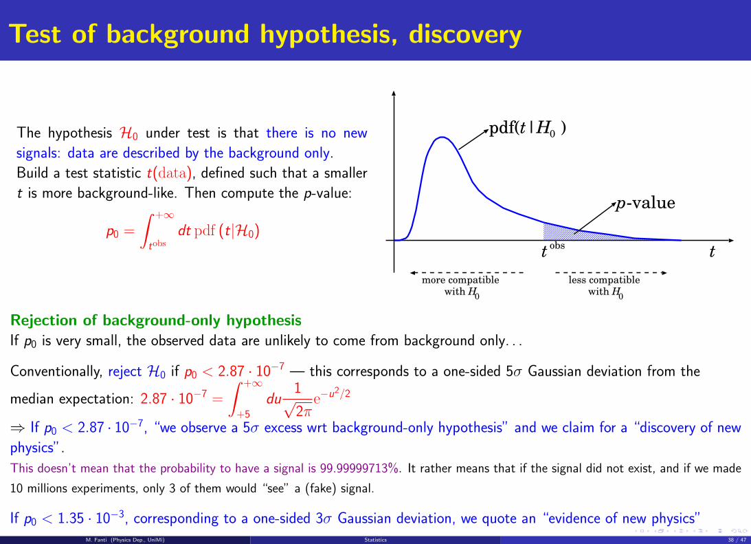
Test of background hypothesis, discovery

The hypothesis H0 under test is that there is no new

signals: data are described by the background only.

Build a test statistic t(data), defined such that a smaller

t is more background-like. Then compute the p-value:

p0 =

∫ +∞

tobsdt pdf (t|H0)

ttobs

p-value

pdf(t|H )0


0

less compatiblewith H

0

Rejection of background-only hypothesisIf p0 is very small, the observed data are unlikely to come from background only. . .

Conventionally, reject H0 if p0 < 2.87 · 10−7 — this corresponds to a one-sided 5σ Gaussian deviation from the

median expectation: 2.87 · 10−7 =

∫ +∞

+5

du1√2π

e−u2/2

⇒ If p0 < 2.87 · 10−7, “we observe a 5σ excess wrt background-only hypothesis” and we claim for a “discovery of new

physics”.

This doesn’t mean that the probability to have a signal is 99.99999713%. It rather means that if the signal did not exist, and if we made

10 millions experiments, only 3 of them would “see” a (fake) signal.

If p0 < 1.35 · 10−3, corresponding to a one-sided 3σ Gaussian deviation, we quote an “evidence of new physics”M. Fanti (Physics Dep., UniMi) Statistics 38 / 47

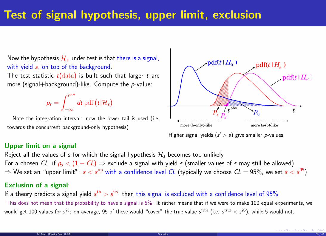
Test of signal hypothesis, upper limit, exclusion

Now the hypothesisHs under test is that there is a signal,

with yield s, on top of the background.

The test statistic t(data) is built such that larger t are

more (signal+background)-like. Compute the p-value:

ps =

∫ tobs

−∞dt pdf (t|Hs)

Note the integration interval: now the lower tail is used (i.e.

towards the concurrent background-only hypothesis)

ttobs

pdf(t|H )0

more (b-only)-like more (s+b)-like

p0

pdf(t|H )s

ps

pdf(t|H )s’

ps’

Higher signal yields (s ′ > s) give smaller p-values

Upper limit on a signal:Reject all the values of s for which the signal hypothesis Hs becomes too unlikely.

For a chosen CL, if ps < (1− CL) ⇒ exclude a signal with yield s (smaller values of s may still be allowed)

⇒ We set an “upper limit”: s < sup with a confidence level CL (typically we choose CL = 95%, we set s < s95)

Exclusion of a signal:If a theory predicts a signal yield sth > s95, then this signal is excluded with a confidence level of 95%

This does not mean that the probability to have a signal is 5%! It rather means that if we were to make 100 equal experiments, we

would get 100 values for s95: on average, 95 of these would “cover” the true value strue (i.e. strue < s95), while 5 would not.


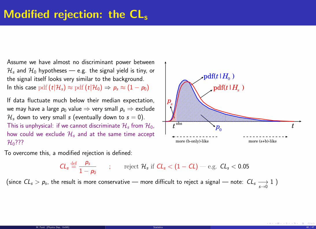
Modified rejection: the CLs

Assume we have almost no discriminant power between

Hs and H0 hypotheses — e.g. the signal yield is tiny, or

the signal itself looks very similar to the background.

In this case pdf (t|Hs) ≈ pdf (t|H0) ⇒ ps ≈ (1− p0)

If data fluctuate much below their median expectation,

we may have a large p0 value⇒ very small ps ⇒ exclude

Hs down to very small s (eventually down to s = 0).

This is unphysical: if we cannot discriminateHs fromH0,

how could we exclude Hs and at the same time accept

H0???

ttobs

pdf(t|H )0

more (b-only)-like more (s+b)-like

p0

pdf(t|H )s

ps

To overcome this, a modified rejection is defined:

CLsdef=

ps1− p0

; reject Hs if CLs < (1− CL) — e.g. CLs < 0.05

(since CLs > ps , the result is more conservative — more difficult to reject a signal — note: CLs −→s→0

1 )


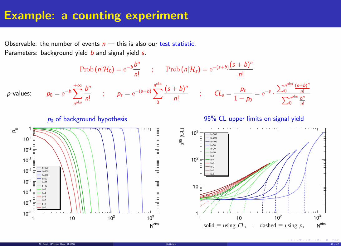
Example: a counting experiment

Observable: the number of events n — this is also our test statistic.

Parameters: background yield b and signal yield s.

Prob (n|H0) = e−bbn

n!; Prob (n|Hs) = e−(s+b) (s + b)n

n!

p-values: p0 = e−b+∞∑nobs

bn

n!; ps = e−(s+b)

nobs∑0

(s + b)n

n!; CLs =

ps1− p0

= e−s ·∑nobs

0(s+b)n

n!∑nobs

0bn

n!

p0 of background hypothesis

obsN

1 10210

310

0p

810

710

610

510

410

310

210

110

1

b=500

b=200

b=100

b=50

b=20

b=10

b=5

b=4

b=3

b=2

b=1

b=0

95% CL upper limits on signal yield

obsN

1 10210

310

(C

L)

95

s

1

10

210

310 b=500

b=200

b=100

b=50

b=20

b=10

b=5

b=4

b=3

b=2

b=1

b=0

solid ≡ using CLs ; dashed ≡ using ps


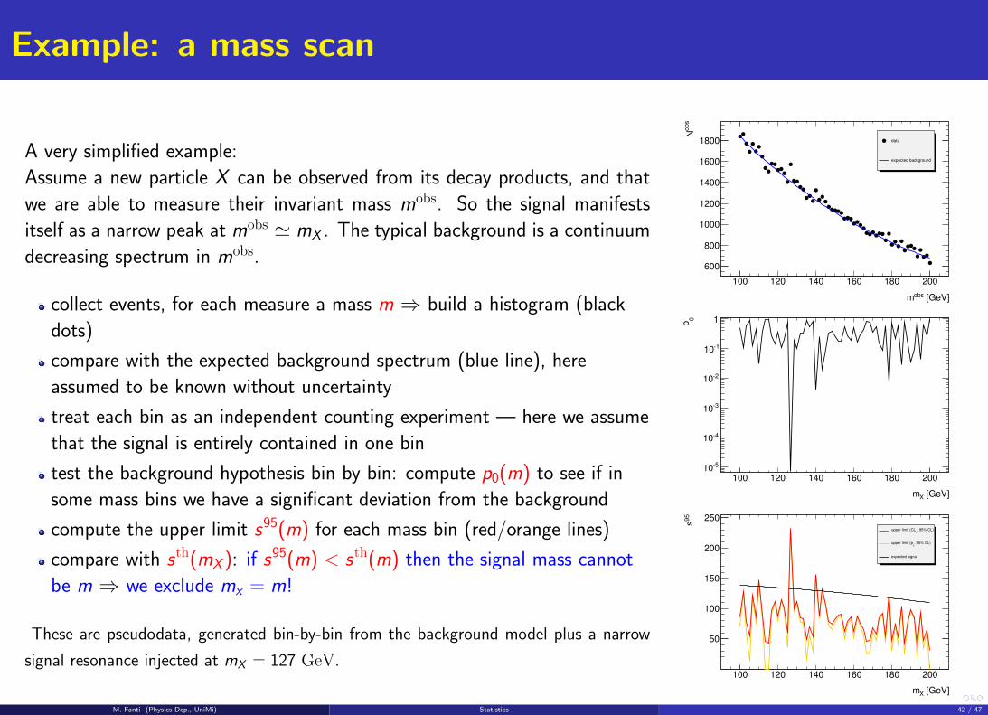
Example: a mass scan

A very simplified example:

Assume a new particle X can be observed from its decay products, and that

we are able to measure their invariant mass mobs. So the signal manifests

itself as a narrow peak at mobs ' mX . The typical background is a continuum

decreasing spectrum in mobs.

collect events, for each measure a mass m ⇒ build a histogram (black

dots)

compare with the expected background spectrum (blue line), here

assumed to be known without uncertainty

treat each bin as an independent counting experiment — here we assume

that the signal is entirely contained in one bin

test the background hypothesis bin by bin: compute p0(m) to see if in

some mass bins we have a significant deviation from the background

compute the upper limit s95(m) for each mass bin (red/orange lines)

compare with sth(mX ): if s95(m) < sth(m) then the signal mass cannot

be m ⇒ we exclude mx = m!

These are pseudodata, generated bin-by-bin from the background model plus a narrow

signal resonance injected at mX = 127 GeV.

[GeV]obsm

100 120 140 160 180 200

ob

sN

600

800

1000

1200

1400

1600

1800 data

expected background

[GeV]Xm

100 120 140 160 180 200

0p

510

410

310

210

110

1

[GeV]Xm

100 120 140 160 180 2009

5s

50

100

150

200

250, 95% CL)

supper limit (CL

, 95% CL)s

upper limit (p

expected signal


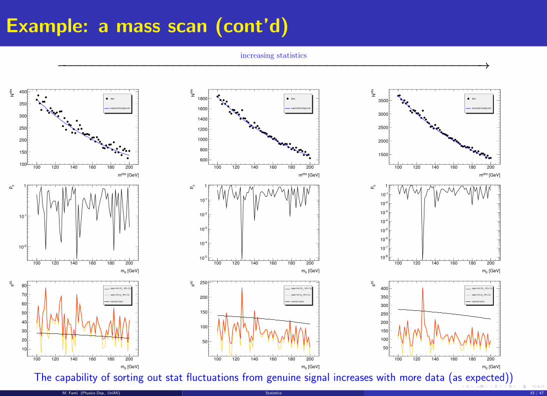
Example: a mass scan (cont’d)

increasing statistics

−−−−−−−−−−−−−−−−−−−−−−−−−−−−−−−−−−−−−−−−−−−−−−−−−−−−−−−−−−→

[GeV]obsm

100 120 140 160 180 200

ob

sN

100

150

200

250

300

350

400

data

expected background

[GeV]Xm

100 120 140 160 180 200

0p

210

110

1

[GeV]Xm

100 120 140 160 180 200

95

s

10

20

30

40

50

60

70

80, 95% CL)

supper limit (CL

, 95% CL)s

upper limit (p

expected signal

[GeV]obsm

100 120 140 160 180 200

ob

sN

600

800

1000

1200

1400

1600

1800 data

expected background

[GeV]Xm

100 120 140 160 180 200

0p

510

410

310

210

110

1

[GeV]Xm

100 120 140 160 180 200

95

s

50

100

150

200

250, 95% CL)

supper limit (CL

, 95% CL)s

upper limit (p

expected signal

[GeV]obsm

100 120 140 160 180 200

ob

sN

1500

2000

2500

3000

3500data

expected background

[GeV]Xm

100 120 140 160 180 200

0p

810

710

610

510

410

310

210

110

1

[GeV]Xm

100 120 140 160 180 200

95

s

50

100

150

200

250

300

350

400 , 95% CL)s

upper limit (CL

, 95% CL)s

upper limit (p

expected signal

The capability of sorting out stat fluctuations from genuine signal increases with more data (as expected))M. Fanti (Physics Dep., UniMi) Statistics 43 / 47

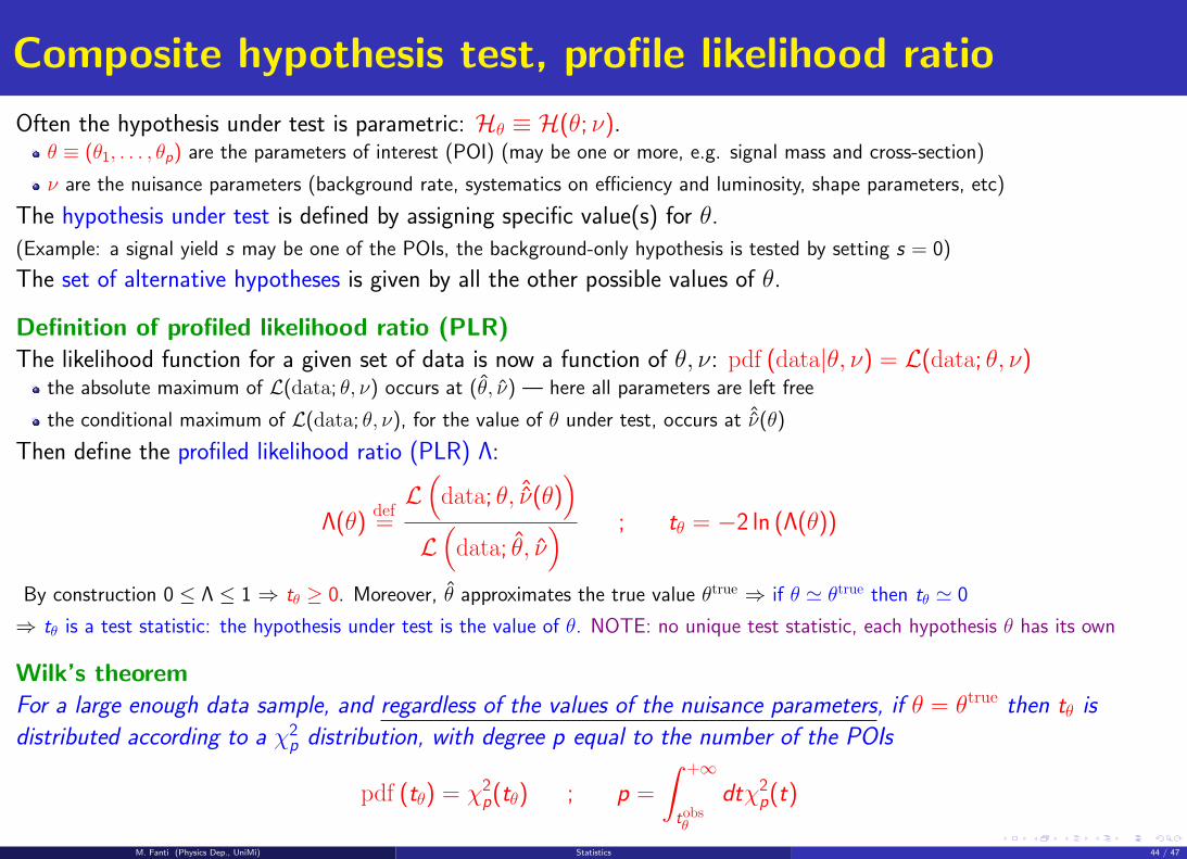
Composite hypothesis test, profile likelihood ratio

Often the hypothesis under test is parametric: Hθ ≡ H(θ; ν).θ ≡ (θ1, . . . , θp) are the parameters of interest (POI) (may be one or more, e.g. signal mass and cross-section)

ν are the nuisance parameters (background rate, systematics on efficiency and luminosity, shape parameters, etc)

The hypothesis under test is defined by assigning specific value(s) for θ.

(Example: a signal yield s may be one of the POIs, the background-only hypothesis is tested by setting s = 0)

The set of alternative hypotheses is given by all the other possible values of θ.

Definition of profiled likelihood ratio (PLR)The likelihood function for a given set of data is now a function of θ, ν: pdf (data|θ, ν) = L(data; θ, ν)

the absolute maximum of L(data; θ, ν) occurs at (θ, ν) — here all parameters are left free

the conditional maximum of L(data; θ, ν), for the value of θ under test, occurs at ˆν(θ)

Then define the profiled likelihood ratio (PLR) Λ:

Λ(θ)def=L(data; θ, ˆν(θ)

)L(data; θ, ν

) ; tθ = −2 ln (Λ(θ))

By construction 0 ≤ Λ ≤ 1 ⇒ tθ ≥ 0. Moreover, θ approximates the true value θtrue ⇒ if θ ' θtrue then tθ ' 0

⇒ tθ is a test statistic: the hypothesis under test is the value of θ. NOTE: no unique test statistic, each hypothesis θ has its own

Wilk’s theoremFor a large enough data sample, and regardless of the values of the nuisance parameters, if θ = θtrue then tθ is

distributed according to a χ2p distribution, with degree p equal to the number of the POIs

pdf (tθ) = χ2p(tθ) ; p =

∫ +∞

tobsθ

dtχ2p(t)


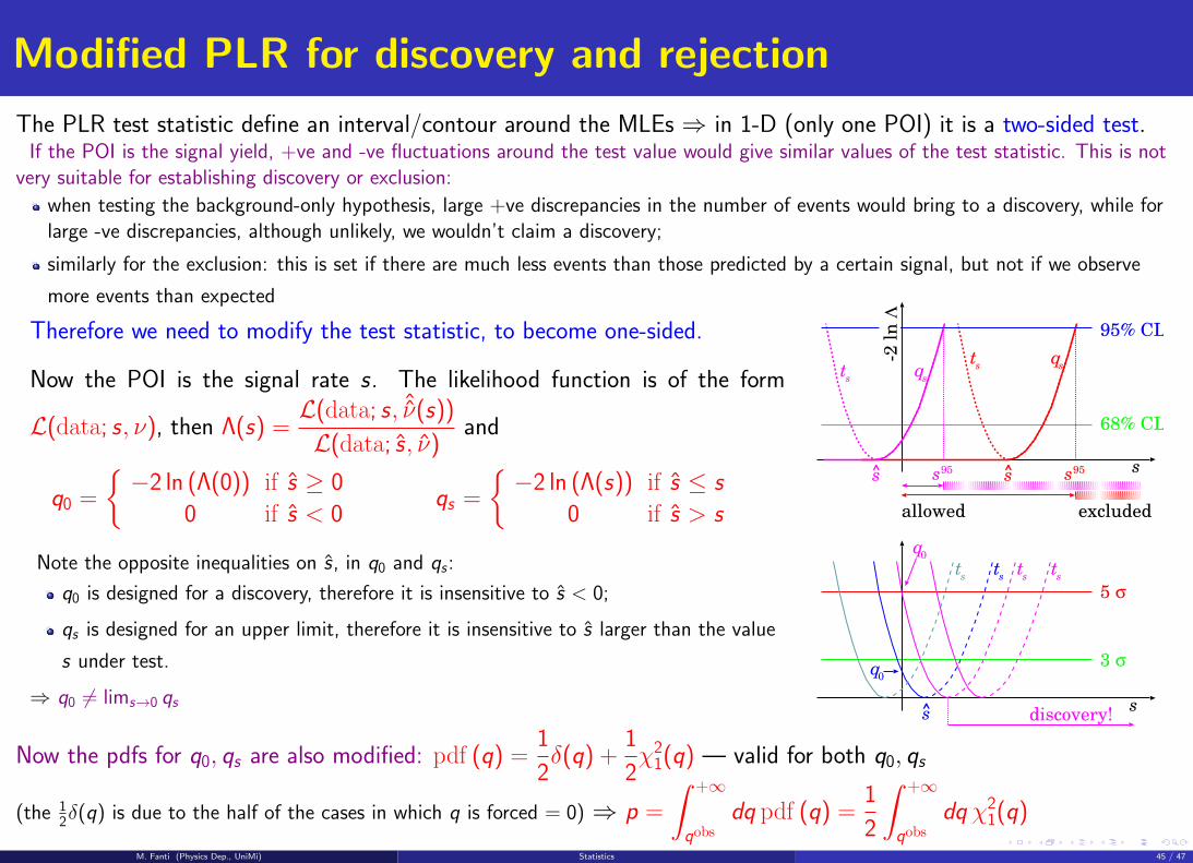
Modified PLR for discovery and rejection

The PLR test statistic define an interval/contour around the MLEs ⇒ in 1-D (only one POI) it is a two-sided test.If the POI is the signal yield, +ve and -ve fluctuations around the test value would give similar values of the test statistic. This is not

very suitable for establishing discovery or exclusion:

when testing the background-only hypothesis, large +ve discrepancies in the number of events would bring to a discovery, while forlarge -ve discrepancies, although unlikely, we wouldn’t claim a discovery;

similarly for the exclusion: this is set if there are much less events than those predicted by a certain signal, but not if we observe

more events than expected

Therefore we need to modify the test statistic, to become one-sided.

Now the POI is the signal rate s. The likelihood function is of the form

L(data; s, ν), then Λ(s) =L(data; s, ˆν(s))

L(data; s, ν)and

q0 =

{−2 ln (Λ(0)) if s ≥ 0

0 if s < 0qs =

{−2 ln (Λ(s)) if s ≤ s

0 if s > s

Note the opposite inequalities on s, in q0 and qs :

q0 is designed for a discovery, therefore it is insensitive to s < 0;

qs is designed for an upper limit, therefore it is insensitive to s larger than the value

s under test.

⇒ q0 6= lims→0 qs

68% CL

95% CL

s

qs

ts

qs

ts

s^ s95s^ s95

5 σ

s^

3 σq

0

discovery!s

excludedallowed

ts

ts

ts

ts

q0

-2 l

n Λ

Now the pdfs for q0, qs are also modified: pdf (q) =1

2δ(q) +

1

2χ2

1(q) — valid for both q0, qs

(the 12δ(q) is due to the half of the cases in which q is forced = 0) ⇒ p =

∫ +∞

qobsdq pdf (q) =

1

2

∫ +∞

qobsdq χ2

1(q)


Combining more channels

Consider a signal that can manifest itself in different channels (e.g. a Higgs boson decaying into different final states

H → γγ, H → W +W− → `ν`ν, H → ZZ → ``νν, H → ZZ → ````). The signal rate s(k) in the k-th channel is

s(k) = µ× L× σth × BR (k) × ε(k)

NOTE: while the total cross-section is allowed to vary by a factor µ (“signal strength modifier”),

in this formulation the braching ratios BR (k) are fixed by the model.

When combining many channels the total likelihood is

L(data;µ, ~ν) =∏k

L(k)(data(k);µ, ~ν(common), ~ν(k)

)

The parameter of interest is now µ : common to all channels

Some nuisance parameters ~ν(common) are also common to all channels (e.g. L, σth)

Other nuisance parameters ~ν(k) are specific of the channel (e.g. ε(k), BR (k), background yields, signal and

background shape parameters. . . )


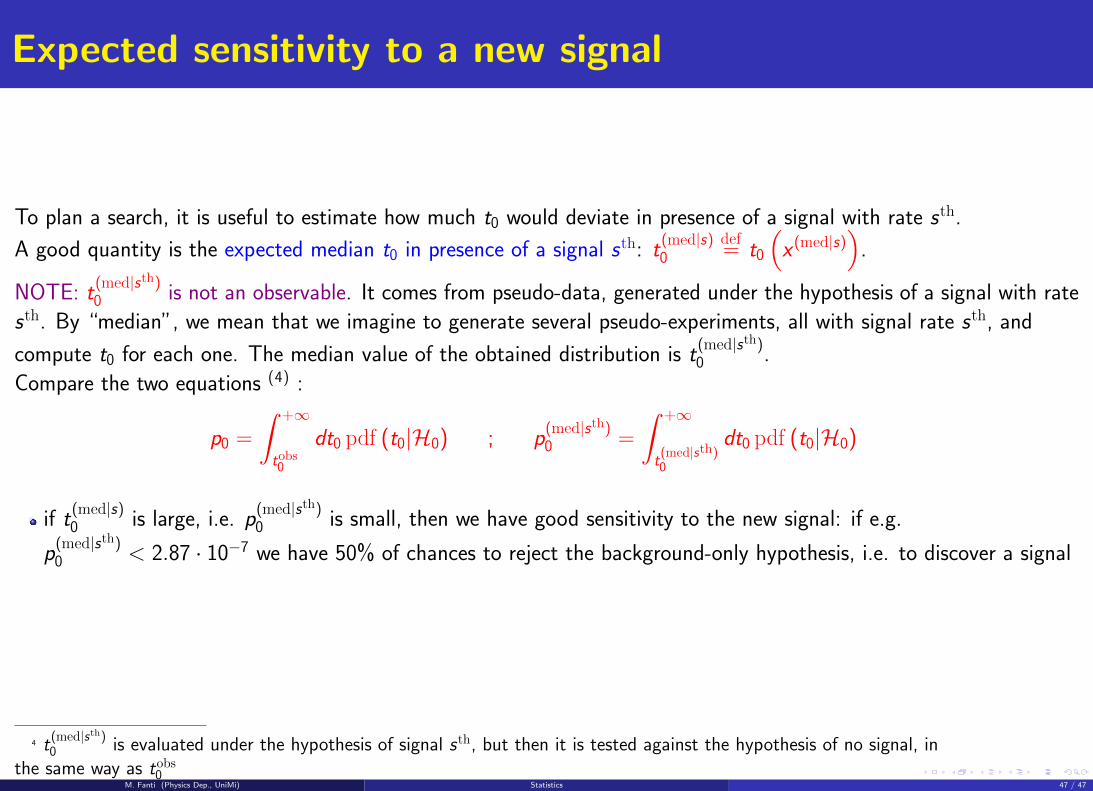
Expected sensitivity to a new signal

To plan a search, it is useful to estimate how much t0 would deviate in presence of a signal with rate sth.

A good quantity is the expected median t0 in presence of a signal sth: t(med|s)0

def= t0

(x (med|s)

).

NOTE: t(med|sth)0 is not an observable. It comes from pseudo-data, generated under the hypothesis of a signal with rate

sth. By “median”, we mean that we imagine to generate several pseudo-experiments, all with signal rate sth, and

compute t0 for each one. The median value of the obtained distribution is t(med|sth)0 .

Compare the two equations (4) :

p0 =

∫ +∞

tobs0

dt0 pdf (t0|H0) ; p(med|sth)0 =

∫ +∞

t(med|sth)0

dt0 pdf (t0|H0)

if t(med|s)0 is large, i.e. p

(med|sth)0 is small, then we have good sensitivity to the new signal: if e.g.

p(med|sth)0 < 2.87 · 10−7 we have 50% of chances to reject the background-only hypothesis, i.e. to discover a signal

4 t(med|sth)0 is evaluated under the hypothesis of signal sth, but then it is tested against the hypothesis of no signal, in

the same way as tobs0M. Fanti (Physics Dep., UniMi) Statistics 47 / 47

Documents

Marcello Fanti - Home INFN Milanofanti/Particelle4/fanti_Statistics.pdf · Statistical techniques Marcello Fanti Physics Dept. | University of Milano M. Fanti (Physics Dep., UniMi)