Geoderma Regional 2–3 (2014) 21–31

Contents lists available at ScienceDirect

Geoderma Regional

j ourna l homepage: www.e lsev ie r .com/ locate /geodrs

Mapping soil salinity changes using remote sensing in Central Iraq

Weicheng Wu a,⁎, Ahmad S. Mhaimeed b, Waleed M. Al-Shafie c, Feras Ziadat a, Boubaker Dhehibi a,Vinay Nangia a, Eddy De Pauw a

a International Center for Agricultural Research in the Dry Areas (ICARDA)/CGIAR, Amman, Jordanb College of Agriculture, Baghdad University, Iraqc Ministry of Agriculture (MoA), Baghdad, Iraq

⁎ Corresponding author at: 11 Avenue Léon Gourdault,E-mail address: wuwc123@gmail.com (W. Wu).

http://dx.doi.org/10.1016/j.geodrs.2014.09.0022352-0094/© 2014 Elsevier B.V. All rights reserved.

a b s t r a c t

a r t i c l e i n f o

Article history:Received 4 April 2014Received in revised form 16 September 2014Accepted 17 September 2014Available online 22 September 2014

Keywords:Salinity dynamicsMultiyear maxima-based modelingMultitemporal remote sensingSoil salinity modelsQuantification in space and time

Salinization is a common problem for agriculture in dryland environments and it has greatly affected land produc-tivity and even caused cropland abandonment in Central and Southern Iraq. Hence it is of pressing importance toquantify the spatial distribution of salinity and its changing trend in space and time and ascertain the driving forcesthereof. This study aims at such a diachronic salinity mapping and analysis using multitemporal remote sensingtaking a pilot site, the Dujaila area in Central Iraq, as an example. For this purpose, field survey and soil samplingwere conducted in the 2011–2012 period, and a multitemporal remote sensing dataset consisting of satellite im-agery dated 1988–1993, 1998–2002, and 2009–2012 was prepared. An innovative processing approach, the mul-tiyear maxima-based modeling approach, was proposed to develop remote sensing salinity models. Afterevaluation of their suitability, the relevantmodelswere applied to the images for multitemporal salinity mapping,quantification, and change tracking in space and time. The driving causes of salinization in the study area wereevaluated. The results reveal that the developed salinity models can reliably predict salinity with an accuracy of82.57%, indicating that ourmappingmethodology is relevant and extendable to other similar environments. In ad-dition, salinity has experienced significant changes in the past 30 years in Dujaila, especially, very strongly sali-nized land got continuously expanded, and all these changes are related to land use practices and managementof farmers, which are closely associated with the macroscopic socioeconomic environment of the country.

© 2014 Elsevier B.V. All rights reserved.

1. Introduction

Salinity is a problematic issue for agriculture in the MesopotamianPlain, Iraq since about 2300–2400 BC (Dieleman, 1963; Schnepf, 2004;FAO, 2011) and has become more severe in the recent decades. It is re-ported that approximately 60% of the cultivated land has been seriouslyaffected by salinity, and 20–30% has been abandoned in the past4000 years (Buringh, 1960; FAO, 2011) due to irrational land manage-ment (e.g., overirrigation and poor drainage) and other natural factors(e.g., flooding, drought, and impermeability of the underlying forma-tion). It is clear that the arable agricultural land would further dwindleinMesopotamia because of such land degradation, andmight be exacer-bated by climate change, and food security would face harsh challengein the country. It is hence of prime importance to quantify the salt-affected land, assess its change trend in space and time, and understandthe causes of salinization in order to provide relevant reference for thelocal and central governments for their sustainable agriculture develop-ment and land management in the future.

In regard of the salinization in Central and Southern Iraq, severalauthors, for example, Jacobsen and Adams (1958), Buringh (1960),

94600 Choisy-Le-Roi, France.

Dieleman (1963), Al-Layla (1978), Al-Mahawili (1983) and Abood et al.(2011) have conducted studies and assessments. These assessmentsallow us to have a general understanding of salinity in theMesopotamianPlain. International organizations such as FAO and UNESCO (United Na-tions Educational, Scientific and Cultural Organization) together withthe Ministry of Agriculture (MoA) of Iraq have carried out soil classifica-tion andmapping in 1960 (Buringh, 1960). FAO (2008) investigated brief-ly the salinity severity in Western Asia including Iraq. However, theoutdating of maps and their extremely low resolution (e.g., 4–10 km inpixel size) cannot meet the requirement of farm-level or household-level land management and for salinity control. Therefore, it is essentialto produce salinity maps with higher resolution, higher accuracy and re-liability to meet the urgent need of farmers and governments.

Salinity assessment and mapping are traditionally conducted by soilsurveys and interpolation of analytical results of soil samples. However,such conventional means of soil survey requires a great deal of time(Ghabour and Daels, 1993) and funding investment. Fortunately, a sig-nificant progress has beenmade in this field thanks to the developmentof remote sensing technology in the recent decades, which offers a pos-sibility for mapping and assessing salinity processes more efficientlyand economically (Garcia et al., 2005). In fact, since the 1970s, a numberof authors namely Hunt et al. (1972), Driessen and Schoorl (1973),Golovina et al. (1992), Steven et al. (1992), Mougenot et al. (1993),

22 W. Wu et al. / Geoderma Regional 2–3 (2014) 21–31

Rao et al. (1995), Metternicht (1998), Metternicht and Zinck (2003),Shao et al. (2003), Douaoui et al. (2006), Farifteh et al. (2006, 2007),Fernández-Buces et al. (2006), Brunner et al. (2007), Rodríguez et al.(2007), Eldeiry andGarcia (2010), Furby et al. (2010) and so on have in-vestigated saline soil-related spectral features and radar signatures, andobtained a number of interesting results, for example, the relationshipsbetween vegetation indices and soil salinity (Steven et al., 1992; Hueteet al., 1997; Garcia et al., 2005; Al-Khaier, 2003; Brunner et al., 2007;Lobell et al., 2010; Iqbal, 2011; Zhang et al., 2011). Some authors haveargued for the possibility to assess salinity using the moisture contentindicator, NDII (Normalized Difference Infrared Index, Hardisky et al.,1983), and the thermal band (Metternicht and Zinck, 1996, 2003;Goossens and van Ranst, 1998; Iqbal, 2011). Recently, Douaoui et al.(2006), Fernández-Buces et al. (2006), Farifteh et al. (2007), Eldeiryand Garcia (2010) and Hu et al. (2014) have proposed respectively theregression-Kriging method, combined spectral response index (COSRI)and best band combination including vegetation index for salinity clas-sification and spatial variability modeling. Others have even discussedthe potential to use SAR (Synthetic Aperture Radar) backscatter coeffi-cients to characterize soil electrical conductivity (Singh and Srivastav,1990; Singh et al., 1990; Taylor et al., 1996; Metternicht, 1998; Shaoet al., 2003).

These studies illustrate not only the advantage, feasibility and greatpotential of remote sensing and GIS in salinity mapping and assessmentbut also challenges to which we need to pay attention. Firstly, salt con-centrated in subsoil is not easily detected by optical remote sensing(Farifteh et al., 2006); even in the topsoil (surface), if the salt contentis below10–15%, it is difficult to be discriminated fromother soil surfacecomponents (Mougenot et al., 1993); however, reflectance increaseswith the increase in quantity of salts at the terrain surface, and this isparticularly true for the blue band, in which the interference causedby ferric oxides is masked (Metternicht and Zinck, 2003). In fact, salt-affected soils show relatively higher spectral response in the visibleand near-infrared regions of the spectrum than non-saline soils, andstrongly saline–sodic soils present higher spectral response than mod-erately saline–sodic soils (Rao et al., 1995; Metternicht and Zinck,2003). Secondly, the moisture in soil contributes to the decrease inreflectance in the middle- and near-infrared bands (Epema, 1990;Mougenot et al., 1993), which can easily lead to misinterpretation ofsalinity if just based on reflectance or vegetation indices. Thirdly, halo-phyte vegetation and even salt-tolerant crops such as barley, cotton,and alfalfa can modify the overall spectral response pattern of salt-affected soils, especially in the green and red bands (Rao et al., 1995;Metternicht, 1998).

We understood from the above brief review that remote sensing is apromising tool, especially, for large-scale salinity assessment. The out-comes of other authors such as relationships established between vege-tation indices, moisture index (e.g. NDII), land surface temperature(LST, from the thermal band) and soil salinity will be useful if they canbe ascertained. However, care should be taken towork out a reasonableapproach for salinity quantification by taking the above challenges intoaccount. In this context, themain objectives of this study are to proposean integrated approach for soil salinity mapping and assessment, trackthe change trend of the salt-affected soils in space and time, and ascer-tain the role of anthropogenic land use practice andmanagement in thesalinization processes. The Dujaila site, a severely salt-affected area inCentral Iraq (Fig. 1), was selected as a pilot site to demonstrate the de-velopment procedure of the integratedmapping approach and its appli-cation for salinity change trend tracking.

2. Materials and methods

2.1. Study site

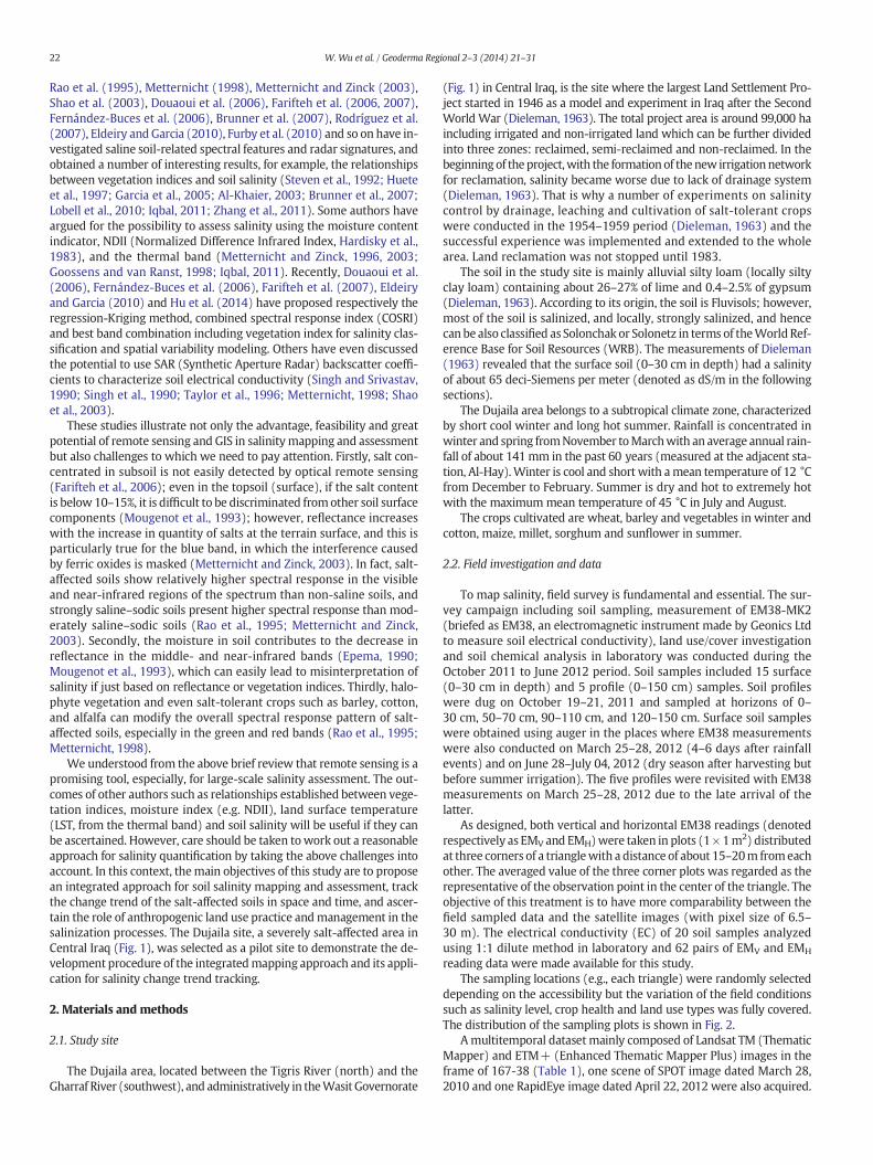
The Dujaila area, located between the Tigris River (north) and theGharraf River (southwest), and administratively in theWasit Governorate

(Fig. 1) in Central Iraq, is the site where the largest Land Settlement Pro-ject started in 1946 as a model and experiment in Iraq after the SecondWorld War (Dieleman, 1963). The total project area is around 99,000 haincluding irrigated and non-irrigated land which can be further dividedinto three zones: reclaimed, semi-reclaimed and non-reclaimed. In thebeginningof theproject,with the formationof thenew irrigationnetworkfor reclamation, salinity became worse due to lack of drainage system(Dieleman, 1963). That is why a number of experiments on salinitycontrol by drainage, leaching and cultivation of salt-tolerant cropswere conducted in the 1954–1959 period (Dieleman, 1963) and thesuccessful experience was implemented and extended to the wholearea. Land reclamation was not stopped until 1983.

The soil in the study site is mainly alluvial silty loam (locally siltyclay loam) containing about 26–27% of lime and 0.4–2.5% of gypsum(Dieleman, 1963). According to its origin, the soil is Fluvisols; however,most of the soil is salinized, and locally, strongly salinized, and hencecan be also classified as Solonchak or Solonetz in terms of theWorld Ref-erence Base for Soil Resources (WRB). The measurements of Dieleman(1963) revealed that the surface soil (0–30 cm in depth) had a salinityof about 65 deci-Siemens per meter (denoted as dS/m in the followingsections).

The Dujaila area belongs to a subtropical climate zone, characterizedby short cool winter and long hot summer. Rainfall is concentrated inwinter and spring fromNovember toMarchwith an average annual rain-fall of about 141mm in the past 60 years (measured at the adjacent sta-tion, Al-Hay).Winter is cool and short with amean temperature of 12 °Cfrom December to February. Summer is dry and hot to extremely hotwith the maximum mean temperature of 45 °C in July and August.

The crops cultivated are wheat, barley and vegetables in winter andcotton, maize, millet, sorghum and sunflower in summer.

2.2. Field investigation and data

To map salinity, field survey is fundamental and essential. The sur-vey campaign including soil sampling, measurement of EM38-MK2(briefed as EM38, an electromagnetic instrument made by Geonics Ltdto measure soil electrical conductivity), land use/cover investigationand soil chemical analysis in laboratory was conducted during theOctober 2011 to June 2012 period. Soil samples included 15 surface(0–30 cm in depth) and 5 profile (0–150 cm) samples. Soil profileswere dug on October 19–21, 2011 and sampled at horizons of 0–30 cm, 50–70 cm, 90–110 cm, and 120–150 cm. Surface soil sampleswere obtained using auger in the places where EM38 measurementswere also conducted on March 25–28, 2012 (4–6 days after rainfallevents) and on June 28–July 04, 2012 (dry season after harvesting butbefore summer irrigation). The five profiles were revisited with EM38measurements on March 25–28, 2012 due to the late arrival of thelatter.

As designed, both vertical and horizontal EM38 readings (denotedrespectively as EMV and EMH)were taken in plots (1× 1m2) distributedat three corners of a trianglewith a distance of about 15–20m fromeachother. The averaged value of the three corner plots was regarded as therepresentative of the observation point in the center of the triangle. Theobjective of this treatment is to have more comparability between thefield sampled data and the satellite images (with pixel size of 6.5–30 m). The electrical conductivity (EC) of 20 soil samples analyzedusing 1:1 dilute method in laboratory and 62 pairs of EMV and EMH

reading data were made available for this study.The sampling locations (e.g., each triangle) were randomly selected

depending on the accessibility but the variation of the field conditionssuch as salinity level, crop health and land use types was fully covered.The distribution of the sampling plots is shown in Fig. 2.

Amultitemporal dataset mainly composed of Landsat TM (ThematicMapper) and ETM+ (Enhanced Thematic Mapper Plus) images in theframe of 167-38 (Table 1), one scene of SPOT image dated March 28,2010 and one RapidEye image dated April 22, 2012 were also acquired.

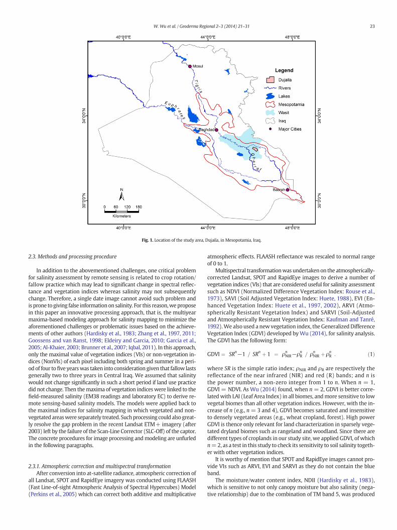
Fig. 1. Location of the study area, Dujaila, in Mesopotamia, Iraq.

23W. Wu et al. / Geoderma Regional 2–3 (2014) 21–31

2.3. Methods and processing procedure

In addition to the abovementioned challenges, one critical problemfor salinity assessment by remote sensing is related to crop rotation/fallow practice which may lead to significant change in spectral reflec-tance and vegetation indices whereas salinity may not subsequentlychange. Therefore, a single date image cannot avoid such problem andis prone to giving false informationon salinity. For this reason,weproposein this paper an innovative processing approach, that is, the multiyearmaxima-based modeling approach for salinity mapping to minimize theaforementioned challenges or problematic issues based on the achieve-ments of other authors (Hardisky et al., 1983; Zhang et al., 1997, 2011;Goossens and van Ranst, 1998; Eldeiry and Garcia, 2010; Garcia et al.,2005; Al-Khaier, 2003; Brunner et al., 2007; Iqbal, 2011). In this approach,only the maximal value of vegetation indices (VIs) or non-vegetation in-dices (NonVIs) of each pixel including both spring and summer in a peri-od of four tofive yearswas taken into consideration given that fallow lastsgenerally two to three years in Central Iraq. We assumed that salinitywould not change significantly in such a short period if land use practicedid not change. Then themaxima of vegetation indiceswere linked to thefield-measured salinity (EM38 readings and laboratory EC) to derive re-mote sensing-based salinity models. The models were applied back tothe maximal indices for salinity mapping in which vegetated and non-vegetated areaswere separately treated. Suchprocessing could also great-ly resolve the gap problem in the recent Landsat ETM+ imagery (after2003) left by the failure of the Scan-Line Corrector (SLC-Off) of the captor.The concrete procedures for image processing andmodeling are unfurledin the following paragraphs.

2.3.1. Atmospheric correction and multispectral transformationAfter conversion into at-satellite radiance, atmospheric correction of

all Landsat, SPOT and RapidEye imagery was conducted using FLAASH(Fast Line-of-sight Atmospheric Analysis of Spectral Hypercubes) Model(Perkins et al., 2005) which can correct both additive and multiplicative

atmospheric effects. FLAASH reflectance was rescaled to normal rangeof 0 to 1.

Multispectral transformationwas undertaken on the atmospherically-corrected Landsat, SPOT and RapidEye images to derive a number ofvegetation indices (VIs) that are considered useful for salinity assessmentsuch as NDVI (Normalized Difference Vegetation Index: Rouse et al.,1973), SAVI (Soil Adjusted Vegetation Index: Huete, 1988), EVI (En-hanced Vegetation Index: Huete et al., 1997, 2002), ARVI (Atmo-spherically Resistant Vegetation Index) and SARVI (Soil-Adjustedand Atmospherically Resistant Vegetation Index: Kaufman and Tanré,1992).We also used a new vegetation index, the Generalized DifferenceVegetation Index (GDVI) developed byWu (2014), for salinity analysis.The GDVI has the following form:

GDVI ¼ SRn−1� �

= SRn þ 1� � ¼ ρn

NIR−ρnR

� �= ρn

NIR þ ρnR

� �: ð1Þ

where SR is the simple ratio index; ρNIR and ρR are respectively thereflectance of the near infrared (NIR) and red (R) bands; and n isthe power number, a non-zero integer from 1 to n. When n = 1,GDVI = NDVI. As Wu (2014) found, when n = 2, GDVI is better corre-latedwith LAI (Leaf Area Index) in all biomes, andmore sensitive to lowvegetal biomes than all other vegetation indices. However, with the in-crease of n (e.g., n= 3 and 4), GDVI becomes saturated and insensitiveto densely vegetated areas (e.g., wheat cropland, forest). High powerGDVI is thence only relevant for land characterization in sparsely vege-tated dryland biomes such as rangeland and woodland. Since there aredifferent types of croplands in our study site, we applied GDVI, of whichn=2, as a test in this study to check its sensitivity to soil salinity togeth-er with other vegetation indices.

It is worthy of mention that SPOT and RapidEye images cannot pro-vide VIs such as ARVI, EVI and SARVI as they do not contain the blueband.

The moisture/water content index, NDII (Hardisky et al., 1983),which is sensitive to not only canopy moisture but also salinity (nega-tive relationship) due to the combination of TM band 5, was produced

Fig. 2. Distribution of the field sampling plots. Note: The background is the multiyear maximal NDVI from Landsat ETM+ images dated 2009–2012. (The SLC-Off gaps were filled. SeeSection 2.3 for procedure.)

24 W. Wu et al. / Geoderma Regional 2–3 (2014) 21–31

from TM and SPOT 4 images, and other non-vegetation indices such asTasseled Cap Brightness (TCB: Crist and Cicone, 1984; Huang et al.,2002; Ivits et al., 2008) and Principal Components (PCs, mainly thefirst and second Principal Components, denoted as PC1 and PC2) werealso derived from Landsat TM and SPOT images (RapidEye can provideonly PCs). These transformations convert land cover information frommultispectral bands into several thematic indicators, e.g., vegetationgreenness and soil moisture. Especially, TCB, an indicator of soil bright-ness, is regarded as an approximation of soil albedo or bulk reflectance.

LST, a useful salinity indicator as Metternicht and Zinck (1996,2003), Goossens and van Ranst (1998) and Iqbal (2011) have revealed,was converted from the thermal band of Landsat TM and ETM+ imagesduring the crop growing period from February to the first half of April(because barley reaches its maturity in the middle of April and is har-vested at the end of the month in Central and Southern Iraq). LST con-version was based on the following equations (Chander et al., 2009):

Lλ ¼ Grescale � Qcal þ Brescale ð2Þ

T ¼ K2=ln K1=Lλð Þ þ 1ð Þ ð3Þ

Table 1Landsat images in the frame with path-row number of 167-38 used in this study.

2010 (2009–2012)(Landsat 7 ETM+)

2000 (1998–2002)(Landsat 5 TM and 7 ETM+)

Spring Summer Spring

2009-03-26 2009-09-02 1998-04-21 (L5)2009-04-11 2010-08-20 2000-03-09 (L5)2010-03-29 2011-08-23 2000-04-26 (L5)2011-04-17 2012-08-25 2001-03-20 (L7)2012-04-03 2001-04-21 (L7)2012-04-19 2002-04-24 (L7)

where Lλ is the spectral radiance at the sensor's aperture [W/(m2 sr μm)];Qcal is the quantized calibrated pixel value in digital number [DN];Grescale is the band-specific rescaling gain factor [(W/(m2 sr μm))/DN];Brescale is the band-specific rescaling bias factor [W/(m2 sr μm)]; andK1 and K2 are calibration coefficients (see Chander et al., 2009 fordetail).

2.3.2. Multiyear datasets and the maxima of VIsA multiyear VI dataset including that from Landsat, SPOT and

RapidEye images was constituted for each VI such as NDVI, SAVI,GDVI, EVI, and SARVI; the same was done for NDII and LST, and theNonVIs namely TCB and PCs (PC1 and PC2). Then the maximal valueof each VI and NonVI in each pixel was extracted by an algorithm de-signed using IDL (Interactive Data Language).

To get a possibly better correlative function with salinity, the vari-ants of the maximal indicators (VIs, NonVIs, NDII and LST) in the formof exponent (exp) and natural logarithm (ln) were derived in con-sideration of the fact that the dependent variable, in our case, the sa-linity, may have better response to the variant(s) of the independentvariable(s).

1990 (1988–1993)(Landsat 4 and 5 TM)

Summer Spring Summer

1999-08-14 (L5) 1988-03-16 (L4) 1990-08-13 (L4)2000-08-08 (L7) 1990-02-18 (L4) 1990-08-29 (L4)2002-07-29 (L7) 1990-03-06 (L4) 1992-08-02 (L4)

1991-03-01 (L5) 1992-08-18 (L4)1993-02-26 (L4)1993-03-30 (L4)

25W. Wu et al. / Geoderma Regional 2–3 (2014) 21–31

2.3.3. Stratification of the vegetated and non-vegetated areasTo separate the vegetated and non-vegetated areas, we used the

multiyear maximal NDVI image by thresholding technique, e.g., givingtentatively a threshold of 0.2 to examine whether it can divide largelythe vegetated and non-vegetated areas while compared with the natu-ral color composite of the original images. If the vegetated-area isoverstated, the threshold should be tuned up (e.g., 0.21, 0.22), other-wise, it should be tuned down, e.g., 0.19, 0.18, till when the best thresh-old is reached. For the multiyear period 2009–2012, it is 0.23, and it is0.21 for 1998–2002, and 0.22 for 1988–1993.

After this division, the sampled data located in different areas can bealso divided into two groups: vegetated and non-vegetated areasamples.

2.3.4. Multiple linear regression analysisA Pearson correlation analysis was firstly applied to understand the

correlation between the EC/EM38 and VIs/NonVIs or that among the VIsand NonVIs. Then the least-square multiple linear regression analysiswas undertaken at the confidence level of 95% to couple the soil EC/EM38 measurements in 2011–2012 with the multiyear maximal VIs,NonVIs and their variants of the 2009–2012 period to obtain the specificsalinity models in the vegetated area, and non-vegetated area, and theintegrated salinity models in the whole study site including both vege-tated and non-vegetated areas. We have to mention that the indepen-dent variables, which were strongly correlated with each other (e.g.R2 N 0.90), were selectively input for modeling, i.e., we selected theones of the best correlation with salinity among all the VIs, togetherwith other non-correlated ones as inputs to avoid auto-correlationproblem among VIs.

NDII and LST have both vegetation and non-vegetation characters,and were integrated in both vegetated and non-vegetated areas for sa-linity modeling.

2.3.5. Evaluation of the models' reliabilityTo understand whether all the models obtained in Section 2.3.4 are

relevant, and reliable for predicting remote sensing-based salinity, it isessential to conduct an evaluation procedure to examine their predictedresults against thefieldmeasured data. To achieve this purpose, the spe-cific VI-based models were applied back to the maximal VIs in the veg-etated area, and NonVI-based models to the maximal NonVIs in thenon-vegetated area, and the integrated models to both VIs and NonVIsof the whole site of the period 2009–2012. The produced maps to beevaluated include (1) those from the integrated models EC-VIs andEMV-VIs without distinction of vegetated and non-vegetated areas;(2) the mosaicked maps from the integrated models EC-VIs or EMV-VIsfor the vegetated area, and EMV/EMH-NonVIs for the non-vegetatedarea; and (3) the mosaicked ones from the specific models for vegetatedand non-vegetated areas.

Theses maps were examined using laboratory measured salinity bylinear regression analysis as was done by Wu et al. (2013) at the confi-dence level of 95%. If the agreement between the map and the groundtruth data is N80% (R2 N 0.8), the predicted salinity map is consideredreliable and the models that we developed are operational.

2.3.6. Multitemporal mapping and salinity change trendsThemost relevant salinitymodels that have been evaluatedwere ap-

plied to the historical multiyear maximal VIs and NonVIs dated 1990(1988–1993) and 2000 (1998–2002) for multitemporal salinity map-ping. As the processing of all historical images was the same as wasdone for the recent ones (the only difference is that there were noSPOT and RapidEye images in the historical datasets), the historical sa-linity maps were regarded reliable although we do not have much his-torical salinity measurement data to validate.

Based on this, the salinity dynamics, change trends in space and timein the recent decades, can be tracked by the differencing technique andthe change in each salinity class was quantified.

2.3.7. Linking salinity change with land use practice and managementBy linking the salinitymaps and change trendwith thefield observa-

tion in land management and household socio-economic survey, a ten-tative analysis to understand the salinization process and causes wasconducted.

3. Results and discussion

3.1. Salinity models

As shown in Table 2, all vegetation indices (including NDII and LST)and their exponential and logarithmic variants are strongly correlatedwith the salinity measured in laboratory (EC) and field EM38 readingsif we take into account both vegetated and non-vegetated areas as a ho-listic site, and GDVI is the best salinity indicator. TCB and PCs, however,show lower correlations with EC and EM38 readings.

Table 3 shows that if we separate vegetated and non-vegetatedareas, the correlation coefficients between EC/EM38 readings and VIsare generally low (R2 b 0.50 for EC-VIs and b0.61 for EMV/EMH-VIs, re-spectively) in the vegetated area, and those in the non-vegetated areabetween EMV/EMH and NonVIs seem better, among which the bestones (e.g., EMH-TCB/PC1) reach 0.74.

Multiple linear regression analysis allowed us to obtain a number ofmodels as listed in Table 4: two integrated models (Model 1: EC-GDVIand Model 2: EMV-GDVI) for the whole study site (without distinctionof vegetated and non-vegetated areas), two integrated models (Model3: EMV-LST/NDII and Model 4: EMH-LST/NDII) for the non-vegetatedarea in which all samples were calibrated with the NonVIs, one specificmodel for the vegetated area (Model 5: EMV-GDVI) based on 43 sam-ples located in the vegetated area, and two specific models (Model 6:EMV-PC1 and Model 7: EMH-TCB) for non-vegetated areas which werederived from 16 samples in the non-vegetated area.

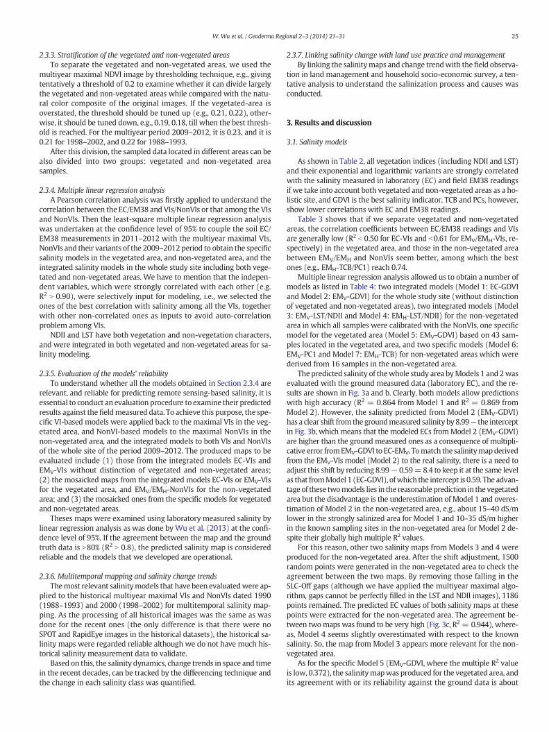
The predicted salinity of thewhole study area byModels 1 and 2wasevaluated with the ground measured data (laboratory EC), and the re-sults are shown in Fig. 3a and b. Clearly, both models allow predictionswith high accuracy (R2 = 0.864 from Model 1 and R2 = 0.869 fromModel 2). However, the salinity predicted from Model 2 (EMV-GDVI)has a clear shift from the groundmeasured salinity by 8.99— the interceptin Fig. 3b, which means that the modeled ECs fromModel 2 (EMV-GDVI)are higher than the ground measured ones as a consequence of multipli-cative error fromEMV-GDVI to EC-EMV. Tomatch the salinitymapderivedfrom the EMV-VIs model (Model 2) to the real salinity, there is a need toadjust this shift by reducing 8.99− 0.59=8.4 to keep it at the same levelas that fromModel 1 (EC-GDVI), ofwhich the intercept is 0.59. The advan-tage of these twomodels lies in the reasonable prediction in the vegetatedarea but the disadvantage is the underestimation of Model 1 and overes-timation of Model 2 in the non-vegetated area, e.g., about 15–40 dS/mlower in the strongly salinized area for Model 1 and 10–35 dS/m higherin the known sampling sites in the non-vegetated area for Model 2 de-spite their globally high multiple R2 values.

For this reason, other two salinity maps from Models 3 and 4 wereproduced for the non-vegetated area. After the shift adjustment, 1500random points were generated in the non-vegetated area to check theagreement between the two maps. By removing those falling in theSLC-Off gaps (although we have applied the multiyear maximal algo-rithm, gaps cannot be perfectly filled in the LST and NDII images), 1186points remained. The predicted EC values of both salinity maps at thesepoints were extracted for the non-vegetated area. The agreement be-tween twomaps was found to be very high (Fig. 3c, R2 = 0.944), where-as, Model 4 seems slightly overestimated with respect to the knownsalinity. So, the map from Model 3 appears more relevant for the non-vegetated area.

As for the specific Model 5 (EMV-GDVI, where the multiple R2 valueis low, 0.372), the salinitymapwas produced for the vegetated area, andits agreement with or its reliability against the ground data is about

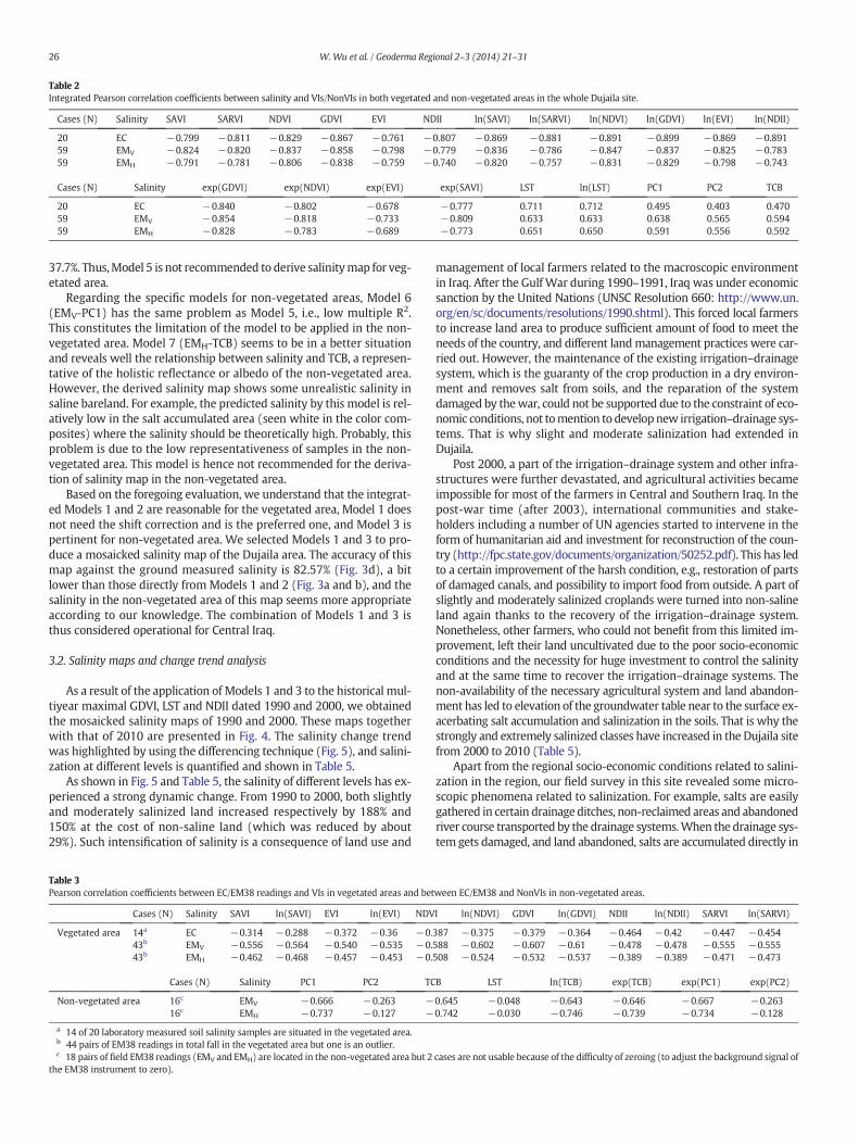
Table 2Integrated Pearson correlation coefficients between salinity and VIs/NonVIs in both vegetated and non-vegetated areas in the whole Dujaila site.

Cases (N) Salinity SAVI SARVI NDVI GDVI EVI NDII ln(SAVI) ln(SARVI) ln(NDVI) ln(GDVI) ln(EVI) ln(NDII)

20 EC −0.799 −0.811 −0.829 −0.867 −0.761 −0.807 −0.869 −0.881 −0.891 −0.899 −0.869 −0.89159 EMV −0.824 −0.820 −0.837 −0.858 −0.798 −0.779 −0.836 −0.786 −0.847 −0.837 −0.825 −0.78359 EMH −0.791 −0.781 −0.806 −0.838 −0.759 −0.740 −0.820 −0.757 −0.831 −0.829 −0.798 −0.743

Cases (N) Salinity exp(GDVI) exp(NDVI) exp(EVI) exp(SAVI) LST ln(LST) PC1 PC2 TCB

20 EC −0.840 −0.802 −0.678 −0.777 0.711 0.712 0.495 0.403 0.47059 EMV −0.854 −0.818 −0.733 −0.809 0.633 0.633 0.638 0.565 0.59459 EMH −0.828 −0.783 −0.689 −0.773 0.651 0.650 0.591 0.556 0.592

26 W. Wu et al. / Geoderma Regional 2–3 (2014) 21–31

37.7%. Thus,Model 5 is not recommended to derive salinitymap for veg-etated area.

Regarding the specific models for non-vegetated areas, Model 6(EMV-PC1) has the same problem as Model 5, i.e., low multiple R2.This constitutes the limitation of the model to be applied in the non-vegetated area. Model 7 (EMH-TCB) seems to be in a better situationand reveals well the relationship between salinity and TCB, a represen-tative of the holistic reflectance or albedo of the non-vegetated area.However, the derived salinity map shows some unrealistic salinity insaline bareland. For example, the predicted salinity by this model is rel-atively low in the salt accumulated area (seen white in the color com-posites) where the salinity should be theoretically high. Probably, thisproblem is due to the low representativeness of samples in the non-vegetated area. This model is hence not recommended for the deriva-tion of salinity map in the non-vegetated area.

Based on the foregoing evaluation, we understand that the integrat-ed Models 1 and 2 are reasonable for the vegetated area, Model 1 doesnot need the shift correction and is the preferred one, and Model 3 ispertinent for non-vegetated area. We selected Models 1 and 3 to pro-duce a mosaicked salinity map of the Dujaila area. The accuracy of thismap against the ground measured salinity is 82.57% (Fig. 3d), a bitlower than those directly from Models 1 and 2 (Fig. 3a and b), and thesalinity in the non-vegetated area of this map seems more appropriateaccording to our knowledge. The combination of Models 1 and 3 isthus considered operational for Central Iraq.

3.2. Salinity maps and change trend analysis

As a result of the application of Models 1 and 3 to the historical mul-tiyear maximal GDVI, LST and NDII dated 1990 and 2000, we obtainedthe mosaicked salinity maps of 1990 and 2000. These maps togetherwith that of 2010 are presented in Fig. 4. The salinity change trendwas highlighted by using the differencing technique (Fig. 5), and salini-zation at different levels is quantified and shown in Table 5.

As shown in Fig. 5 and Table 5, the salinity of different levels has ex-perienced a strong dynamic change. From 1990 to 2000, both slightlyand moderately salinized land increased respectively by 188% and150% at the cost of non-saline land (which was reduced by about29%). Such intensification of salinity is a consequence of land use and

Table 3Pearson correlation coefficients between EC/EM38 readings and VIs in vegetated areas and bet

Cases (N) Salinity SAVI ln(SAVI) EVI ln(EVI) NDV

Vegetated area 14a EC −0.314 −0.288 −0.372 −0.36 −0.43b EMV −0.556 −0.564 −0.540 −0.535 −0.43b EMH −0.462 −0.468 −0.457 −0.453 −0.

Cases (N) Salinity PC1 PC2 TC

Non-vegetated area 16c EMV −0.666 −0.263 −16c EMH −0.737 −0.127 −

a 14 of 20 laboratory measured soil salinity samples are situated in the vegetated area.b 44 pairs of EM38 readings in total fall in the vegetated area but one is an outlier.c 18 pairs of field EM38 readings (EMV and EMH) are located in the non-vegetated area but 2

the EM38 instrument to zero).

management of local farmers related to the macroscopic environmentin Iraq. After the Gulf War during 1990–1991, Iraq was under economicsanction by the United Nations (UNSC Resolution 660: http://www.un.org/en/sc/documents/resolutions/1990.shtml). This forced local farmersto increase land area to produce sufficient amount of food to meet theneeds of the country, and different landmanagement practices were car-ried out. However, the maintenance of the existing irrigation–drainagesystem, which is the guaranty of the crop production in a dry environ-ment and removes salt from soils, and the reparation of the systemdamaged by thewar, could not be supported due to the constraint of eco-nomic conditions, not tomention to developnew irrigation–drainage sys-tems. That is why slight and moderate salinization had extended inDujaila.

Post 2000, a part of the irrigation–drainage system and other infra-structures were further devastated, and agricultural activities becameimpossible for most of the farmers in Central and Southern Iraq. In thepost-war time (after 2003), international communities and stake-holders including a number of UN agencies started to intervene in theform of humanitarian aid and investment for reconstruction of the coun-try (http://fpc.state.gov/documents/organization/50252.pdf). This has ledto a certain improvement of the harsh condition, e.g., restoration of partsof damaged canals, and possibility to import food from outside. A part ofslightly and moderately salinized croplands were turned into non-salineland again thanks to the recovery of the irrigation–drainage system.Nonetheless, other farmers, who could not benefit from this limited im-provement, left their land uncultivated due to the poor socio-economicconditions and the necessity for huge investment to control the salinityand at the same time to recover the irrigation–drainage systems. Thenon-availability of the necessary agricultural system and land abandon-ment has led to elevation of the groundwater table near to the surface ex-acerbating salt accumulation and salinization in the soils. That is why thestrongly and extremely salinized classes have increased in the Dujaila sitefrom 2000 to 2010 (Table 5).

Apart from the regional socio-economic conditions related to salini-zation in the region, our field survey in this site revealed some micro-scopic phenomena related to salinization. For example, salts are easilygathered in certain drainage ditches, non-reclaimed areas and abandonedriver course transported by the drainage systems.When the drainage sys-tem gets damaged, and land abandoned, salts are accumulated directly in

ween EC/EM38 and NonVIs in non-vegetated areas.

I ln(NDVI) GDVI ln(GDVI) NDII ln(NDII) SARVI ln(SARVI)

387 −0.375 −0.379 −0.364 −0.464 −0.42 −0.447 −0.454588 −0.602 −0.607 −0.61 −0.478 −0.478 −0.555 −0.555508 −0.524 −0.532 −0.537 −0.389 −0.389 −0.471 −0.473

B LST ln(TCB) exp(TCB) exp(PC1) exp(PC2)

0.645 −0.048 −0.643 −0.646 −0.667 −0.2630.742 −0.030 −0.746 −0.739 −0.734 −0.128

cases are not usable because of the difficulty of zeroing (to adjust the background signal of

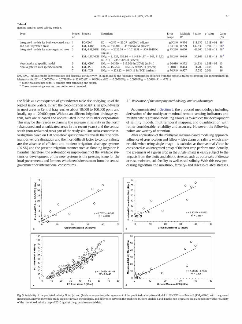
Table 4Remote sensing-based salinity models.

Type Modelno.

Models Equations Errorscope

MultipleR2

F-ratio p-Value Cases(N)

Integrated models for both vegetated areaand non-vegetated areas

1 EC-GDVI EC = −2.87 − 23.27 ln(GDVI) (dS/m) ±5.240 0.874 111.137 1.31E−08 19a

2 EMV-GDVI EMV = 535.403 − 487.905GDVI (mS/m) ±64.168 0.729 142.839 9.99E−16 58b

Integrated models for non-vegetated area 3 EMV-LST/NDII EMV = −2725.05 + 10.018LST − 509.494NDII(mS/m)

±73.230 0.650 47.360 2.36E−12 58b

4 EMH-LST/NDII EMH = 1, 627, 956.14 + 1148.84LST − 345, 815.62ln(LST) − 245.198NDII (mS/m)

±58.240 0.649 30.869 1.95E−11 58b

Vegetated area specific model 5 EMV-GDVI EMV = 64.359 − 319.306 ln(GDVI) (mS/m) ±54.680 0.372 24.331 1.39E−05 43Non-vegetated area specific models 6 EMV-PC1 EMV = 1502.43 − 1166.35 exp(PC1) (mS/m) ±90.811 0.444 11.200 0.005 16

7 EMH-TCB EMH = −223.22 − 1043.11 ln(TCB) (mS/m) ±74.549 0.557 17.585 0.001 16

EMV/EMH (mS/m) can be converted into soil electrical conductivity (EC in dS/m) by the following relationships obtained from the regional transect sampling and measurement inMesopotamia: EC = 0.0005EMV

2 − 0.0779EMV + 12.655 (R2 = 0.850) and EC = 0.0002EMH2 + 0.0956EMH + 0.0688 (R2 = 0.791).

a Model was obtained with 19 samples after removing one outlier.b Three non-zeroing cases and one outlier were removed.

27W. Wu et al. / Geoderma Regional 2–3 (2014) 21–31

the fields as a consequence of groundwater table rise or drying-up of thelogged saline waters. In fact, the concentration of salt(s) in groundwaterin most areas in Central Iraq reaches about 10,000 to 100,000 ppm, andlocally, up to 120,000 ppm. Without an efficient irrigation–drainage sys-tem, salts are released and accumulated in the soils after evaporation.This may be the reason explaining the increase in salinity in the north(abandoned and uncultivated areas in the recent years) and the centralsouth (non-reclaimed area) part of the study site. Our socio-economic in-vestigation based on 150 household questionnaires reveals that the dom-inant driver of salinization and the most difficult factor to control salinityare the absence of efficient and modern irrigation–drainage systems(97.5%) and the present irrigation manner such as flooding irrigation isharmful. Therefore, the restoration or improvement of the available sys-tems or development of the new systems is the pressing issue for thelocal governments and farmers, which needs investment from the centralgovernment or international consortiums.

Fig. 3. Reliability of the predicted salinity. Note: (a) and (b) show respectively the agreement ofmeasured salinity in thewhole study area; (c) reveals the similarity and difference between theof the mosaicked salinity map of 2010 against the ground measured data.

3.3. Relevance of the mapping methodology and its advantages

As demonstrated in Section 2, the proposed methodology includingderivation of the multiyear maximal remote sensing indicators andmultivariate regressionmodeling allows us to achieve the developmentof salinity models, multitemporal mapping and quantification withrather considerable reliability and accuracy. However, the followingpoints are worthy of attention.

After application of the multiyear maxima-based modeling approach,influence of crop rotation and fallow – false alarm on salinity which is in-evitable when using single image – is excluded as the maximal VI can beconsidered as an integrated proxy of the best crop performance. Actually,the greenness of a given crop in the single image is easily subject to theimpacts from the biotic and abiotic stresses such as outbreaks of diseaseor rust, moisture, soil fertility as well as soil salinity. With this new pro-cessing algorithm, the moisture-, fertility- and disease-related stresses,

the predicted salinity fromModel 1 (EC-GDVI) andModel 2 (EMV-GDVI)with the groundpredicted EC fromModels 3 and 4 in the non-vegetated area; and (d) shows the reliability

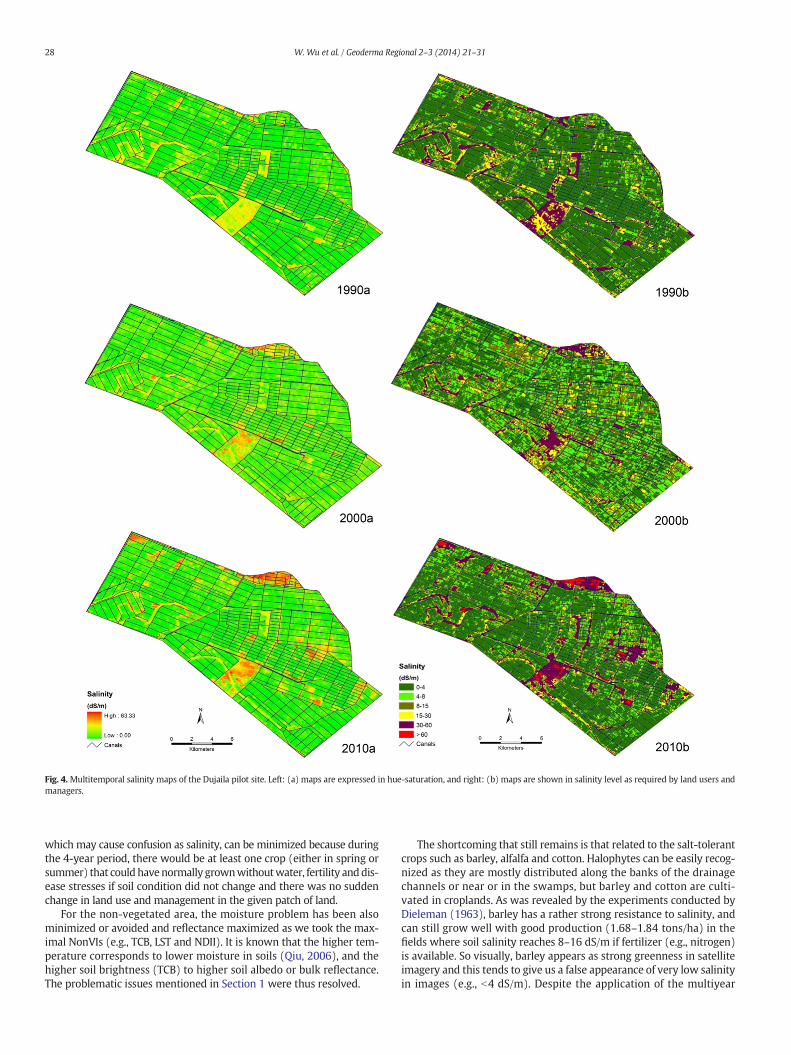
Fig. 4.Multitemporal salinity maps of the Dujaila pilot site. Left: (a) maps are expressed in hue-saturation, and right: (b) maps are shown in salinity level as required by land users andmanagers.

28 W. Wu et al. / Geoderma Regional 2–3 (2014) 21–31

which may cause confusion as salinity, can be minimized because duringthe 4-year period, there would be at least one crop (either in spring orsummer) that couldhavenormally grownwithoutwater, fertility anddis-ease stresses if soil condition did not change and there was no suddenchange in land use and management in the given patch of land.

For the non-vegetated area, the moisture problem has been alsominimized or avoided and reflectance maximized as we took the max-imal NonVIs (e.g., TCB, LST and NDII). It is known that the higher tem-perature corresponds to lower moisture in soils (Qiu, 2006), and thehigher soil brightness (TCB) to higher soil albedo or bulk reflectance.The problematic issues mentioned in Section 1 were thus resolved.

The shortcoming that still remains is that related to the salt-tolerantcrops such as barley, alfalfa and cotton. Halophytes can be easily recog-nized as they are mostly distributed along the banks of the drainagechannels or near or in the swamps, but barley and cotton are culti-vated in croplands. As was revealed by the experiments conducted byDieleman (1963), barley has a rather strong resistance to salinity, andcan still grow well with good production (1.68–1.84 tons/ha) in thefields where soil salinity reaches 8–16 dS/m if fertilizer (e.g., nitrogen)is available. So visually, barley appears as strong greenness in satelliteimagery and this tends to give us a false appearance of very low salinityin images (e.g., b4 dS/m). Despite the application of the multiyear

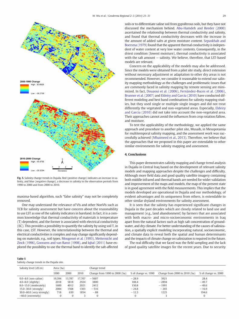
Fig. 5. Salinity change trends in Dujaila. Red (positive change) indicates an increase in sa-linity, and blue (negative change), a decrease in salinity in the observation periods from1990 to 2000 and from 2000 to 2010.

29W. Wu et al. / Geoderma Regional 2–3 (2014) 21–31

maxima-based algorithm, such “false salinity” may not be completelyremoved.

One may understand the relevance of VIs and other NonVIs such asTCB for salinity assessment but have concern about the reasonabilityto use LST as one of the salinity indicators in bareland. In fact, it is a com-mon knowledge that thermal conductivity of materials is temperature(T) dependent, and the former is associated with electrical conductivity(EC). This provides a possibility to quantify the salinity by using soil T, inthis case, LST. However, the interrelationship between the thermal andelectrical conductivities is complex andmay change significantly depend-ing on materials, e.g., soil types. Mougenot et al. (1993), Metternicht andZinck (1996), Goossens and van Ranst (1998), and Iqbal (2011) have ex-plored the possibility to use the thermal band to identify the salt-affected

Table 5Salinity change trends in the Dujaila site.

Salinity level (dS/m) Area (ha) Change trend

1990 2000 2010 Change from 1990 to 2000 (h

0.0–4.0 (non-saline) 19,394 13,787 17,707 −56074.0–8.0 (slightly) 2018 5818 2924 38008.0–15.0 (moderately) 1600 4012 2021 241215.0–30.0 (strongly) 2084 1568 1303 −51630.0–60.0 (very strongly) 718 630 1854 −88N60.0 (extremely) 0 0 3 0

soils or to differentiate saline soil fromgypsiferous soils, but they have notdiscussed the mechanism behind. Abu-Hamdeh and Reeder (2000)ascertained the relationship between thermal conductivity and salinity,and found that thermal conductivity decreases with the increase inthe amount of added salts at given moisture content. Sepaskhah andBoersma (1979) found that the apparent thermal conductivity is indepen-dent of water content at very low water contents. Consequently, in thedriest condition (lowest moisture), thermal conductivity is associatedwith the salt amount — salinity. We believe, therefore, that LST-basedmodels are relevant.

Concern on the applicability of the models may also be addressed.Since themodels were obtained from a pilot site study, direct extensionwithout necessary adjustment or adaptation to other dry areas is notrecommended. However, we consider it reasonable to extend our salin-ity mappingmethodology as the challenges and problematic issues thatare commonly faced in salinity mapping by remote sensing are mini-mized. In fact, Douaoui et al. (2006), Fernández-Buces et al. (2006),Brunner et al. (2007) and Eldeiry andGarcia (2010) have conducted dif-ferent modeling and best band combinations for salinity mapping stud-ies, but they used single or multiple single images and did not treatdifferently the vegetated and non-vegetated areas. Especially, Eldeiryand Garcia (2010) did not take into account the non-vegetated area.Their approaches cannot avoid the influences from crop rotation/fallow,and moisture.

To test the applicability of the methodology, we applied the sameapproach and procedure to another pilot site, Musaib, in Mesopotamiafor multitemporal salinity mapping, and the assessment work was suc-cessfully achieved (Mhaimeed et al., 2013). Therefore, we believe thatthe approaches that we proposed in this paper are extendable to othersimilar environments for salinity mapping and assessment.

4. Conclusions

This paper demonstrates salinitymapping and change trend analysisin Dujaila in Central Iraq based on the development of relevant salinitymodels and mapping approaches despite the challenges and difficulty.Although more field data and good quality satellite imagery containingbothmiddle infrared and thermal bands are needed forwider validationand improvement of themaps andmodels, themap of the present stateis in good agreementwith the fieldmeasurements. This implies that themodels developed are operational in Dujaila and our methodology, ofevident advantages and its uniqueness from others, is extendable toother similar dryland environments for salinity assessment.

It is seen that the salinity has experienced significant changes inDujaila in the past decades which are closely related to land use andmanagement (e.g., land abandonment) by farmers that are associatedwith both macro- and micro-socioeconomic environments in Iraqapart from the natural factors such as high salt concentration of ground-water, and dry climate. For better understanding of the causes of saliniza-tion, a spatially explicit modeling incorporating natural, socioeconomic,and climate data to reveal both the spatial and human determinantsand the impacts of climate change on salinization is required in the future.

The real difficulty that we faced was the field sampling and the lackof good quality satellite images for the recent years. Due to security

a) % of change vs. 1990 Change from 2000 to 2010 (ha) % of change vs. 2000

−28.9 3921 28.4188.4 −2894 −49.7150.8 −1991 −49.6−24.8 −265 −16.9−12.3 1225 194.6

0 3 0

30 W. Wu et al. / Geoderma Regional 2–3 (2014) 21–31

reasons, a number of designed sampling plotswere not accessible, espe-cially in barelands. Instead of random sampling, a stratified sampling isenvisaged when the security situation improves. Additionally, LandsatETM+ images were themain source that we could utilize for the recentperiod. Due to the SLC-Off problem, these images, especially, the short-wave infrared and thermal bandswere not ideal thoughwe had appliedthe maxima-based algorithm. In future work, we should use Landsat 8data as they have become available since April 2013.

Acknowledgments

The study was funded by the Australian Centre for International Ag-ricultural Research (ACIAR) [Project No: LWR/2009/034]. All Landsatimages were freely obtained from the USGS data server (http://glovis.usgs.gov). The RapidEye image was provided byMr Clemens Stromeyer(RapidEye AG). A sincere thank is due to Dr Ayad A. Hameed, Dr HassanH. Al-Musawi (Ministry of Water Resources of Iraq), and Ms BinanDardar (ICARDA) for their assistance in field sampling and partiallyimage processing. Gratitude will also go to Dr Kasim A. Saliem (Ministryof Agriculture of Iraq), Mr Alexander Platonov (IWMI-Tashkent), DrEvan Christen (CSIRO), Dr Manzoor Qadir (UNU-INWEH), and Dr TheibOweis (ICARDA) for their cooperation in the early stage of the work.

Appendix A. Supplementary data

Supplementary data associated with this article can be found in theonline version, at http://dx.doi.org/10.1016/j.geodrs.2014.09.002. Thesedata include Google maps of the most important areas described in thisarticle.

References

Abood, S., Maclean, A., Falkowski, M., 2011. Soil salinity detection in the Mesopotamianagricultural plain utilizing WorldView-2 imageryAvailable at: http://dgl.us.neolane.net/res/img/16bb89b080930a8ad1fdfc17665883e9.pdf.

Abu-Hamdeh, N.H., Reeder, R.C., 2000. Soil thermal conductivity effects of density, mois-ture, salt concentration, and organicmatter. Soil Sci. Soc. Am. J. 64, 1285–1290. http://dx.doi.org/10.2136/sssaj2000.6441285x.

Al-Khaier, F., 2003. Soil Salinity Detection Using Satellite Remote Sensing(MS Thesis) ITC(International Institute for Geo-information Science and Earth Observation), TheNetherlands.

Al-Layla, M.A., 1978. Effect of salinity on agriculture in Iraq. J. Irrig. Drain. Div. 104 (2),195–207.

Al-Mahawili, S.M.H., 1983. Satellite Image Interpretation and Laboratory Spectral Reflec-tance Measurement of Saline and Gypsiferous Soils of West Baghdad(M.Sc Thesis)Purdue University, Iraq.

Brunner, P., Li, H.T., Kinzelbach, W., Li, W.P., 2007. Generating soil electrical conductivitymaps at regional level by integrating measurements on the ground and remote sens-ing data. Int. J. Remote Sens. 28, 3341–3361.

Buringh, P., 1960. Soils and Soil Conditions in Iraq. Ministry of Agriculture of Iraq, (337 pp.).Chander, G., Markham, B.L., Helder, D.L., 2009. Summary of current radiometric calibra-

tion coefficients for Landsat MSS, TM, ETM+, and EO-1 ALI sensors. Remote Sens. En-viron. 113, 893–903.

Crist, E.P., Cicone, R.C., 1984. Application of the tasseled cap concept to simulated thematicmapper data. Photogramm. Eng. Remote. Sens. 50, 343–352.

Dieleman, P.J. (Ed.), 1963. Reclamation of Salt Affected Soils in Iraq. International Institutefor Land Reclamation and Improvement, Wageningen Publication (175 pp.).

Douaoui, A.E.K., Nicolas, H., Walter, C., 2006. Detecting salinity hazards within a semiaridcontext by means of combining soil and remote-sensing data. Geoderma 134,217–230.

Driessen, P.M., Schoorl, R., 1973. Mineralogy and morphology of salt efflorescences on sa-line soils in the Great Konya Basin, Turkey. J. Soil Sci. 24, 436–442.

Eldeiry, A.A., Garcia, L.A., 2010. Comparison of ordinary kriging, regression kriging, andcokriging techniques to estimate soil salinity using Landsat images. J. Irrig. Drain.Eng. 136, 355–364.

Epema, G.F., 1990. Effect of moisture content on spectral reflectance in a playa area insouthern Tunisia. Proc. International Symposium on Remote Sensing and Water Re-sources, Enschede. International Institute for Aerospace Survey and Earth Sciences,The Netherlands, pp. 301–308.

FAO, 2008. Irrigation in the Middle East Region in figures. FAO Water Reports 34.AQUASTAT Survey, p. 423.

FAO, 2011. Country Pasture/Forage Resource Profiles: Iraq. FAO, Rome, Italy, p. 34.Farifteh, J., Farshad, A., George, R.J., 2006. Assessing salt-affected soils using remote sens-

ing, solute modelling, and geophysics. Geoderma 130 (3–4), 191–206.

Farifteh, J., van der Meer, F., Atzberger, C., Carranza, E., 2007. Quantitative analysis of salt-affected soil reflectance spectra: a comparison of two adaptive methods (PLSR andANN). Remote Sens. Environ. 110, 59–78.

Fernández-Buces, N., Siebe, C., Cram, S., Palacio, J.L., 2006. Mapping soil salinity using acombined spectral response index for bare soil and vegetation: a case study in theformer lake Texcoco, Mexico. J. Arid Environ. 65, 644–667.

Furby, S., Caccetta, P., Wallace, J., 2010. Salinity monitoring in Western Australia using re-motely sensed and other spatial data. J. Environ. Qual. 39, 16–25.

Garcia, L., Eldeiry, A., Elhaddad, A., 2005. Estimating soil salinity using remote sensingdata. Proceedings of the 2005 Central Plains Irrigation Conference, pp. 1–10 (availableat: http://www.ksre.ksu.edu/irrigate/OOW/P05/Garcia.pdf; accessed on Jan 2013).

Ghabour, T.K., Daels, L., 1993. Mapping andmonitoring of soil salinity of ISSN. Egypt. J. SoilSci. 33 (4), 355–370.

Golovina, N.N., Minskiy, D., Pankova, Y., Solovyev, D.A., 1992. Automated air photo inter-pretation in the mapping of soil salinization in cotton-growing zones. Mapp. Sci. Re-mote. Sens. 29, 262–268.

Goossens, R., van Ranst, E., 1998. The use of remote sensing tomap gypsiferous soils in theIsmailia Province (Egypt). Geoderma 87, 47–56.

Hardisky, M.A., Klemas, V., Smart, R.M., 1983. The influences of soil salinity, growth form,and leaf moisture on the spectral reflectance of Spartina alterniflora canopies.Photogramm. Eng. Remote Sens. 49, 77–83.

Hu, W., Shao, M.A., Wan, L., Si, B.C., 2014. Spatial variability of soil electrical conductivityin a small watershed on the Loess Plateau of China. Geoderma 230–231, 212–220.

Huang, C., Wylie, B., Yang, L., Homer, C., Zylstra, G., 2002. Derivation of a tasseled captransformation based on Landsat 7 at-satellite reflectance. Int. J. Remote Sens. 23,1741–1748.

Huete, A.R., 1988. A soil adjusted vegetation index (SAVI). Remote Sens. Environ. 25,295–309.

Huete, A.R., Liu, H.Q., Batchily, K., van Leeuwen, W., 1997. A comparison of vegetation in-dices global set of TM images for EOS-MODIS. Remote Sens. Environ. 59, 440–451.

Huete, A.R., Didan, K., Miura, T., Rodriguez, E.P., Gao, X., Ferreira, L.G., 2002. Overview ofthe radiometric and biophysical performance of the MODIS vegetation indices. Re-mote Sens. Environ. 83, 195–213.

Hunt, G., Salisbury, J., Lenhoff, C., 1972. Visible and near infrared spectra of minerals androcks: V. Halides, phosphates, arsenates, venadates and borates. Mod. Geol. 3,121–132.

Iqbal, F., 2011. Detection of salt affected soil in rice–wheat area using satellite image. Afr.J. Agric. Res. 6, 4973–4982.

Ivits, E., Lamb, A., Langar, F., Hemphill, S., Koch, B., 2008. Orthogonal transformation ofsegmented SPOT5 images: seasonal and geographical dependence of the tasselledcap parameters. Photogramm. Eng. Remote Sens. 74 (11), 1351–1364.

Jacobsen, T., Adams, R.M., 1958. Salt and silt in ancient Mesopotamian agriculture. Science128, 1251–1258.

Kaufman, Y.J., Tanré, D., 1992. Atmospherically resistant vegetation index (ARVI) for EOS-MODIS. IEEE Trans. Geosci. Remote Sens. 30, 261–270.

Lobell, D.B., Lesch, S.M., Corwin, D.L., Ulmer, M.G., Anderson, K.A., Potts, D.J., Doolittle, J.A.,Matos, M.R., Baltes, M.J., 2010. Regional-scale assessment of soil salinity in the redriver valley using multi-year MODIS EVI and NDVI. J. Environ. Qual. 39, 35–41.

Metternicht, G., 1998. Analysing the relationship between ground based reflectance andenvironmental indicators of salinity processes in the Cochabamba Valleys (Bolivia).Int. J. Ecol. Environ. Sci. 24, 359–370.

Metternicht, G.I., Zinck, J.A., 1996. Modelling salinity–alkalinity classes for mapping salt-affected topsoils in the semi-arid valleys of Cochabamba (Bolivia). ITC J. 1996 (2),125–135.

Metternicht, G.I., Zinck, J.A., 2003. Remote sensing of soil salinity: potentials and con-straints. Remote Sens. Environ. 85, 1–20.

Mhaimeed, A., Wu, W., AL-Shafie, W., Ziadat, F., Al-Musawi, H., Kasim, A.S., 2013. Use re-mote sensing to map soil salinity in the Musaib Area in Central Iraq. Int. J. Geosci.Geomatics 1 (2), 34–41 (ISSN 2052-5591).

Mougenot, B., Pouget, M., Epema, G., 1993. Remote sensing of salt-affected soils. RemoteSens. Rev. 7, 241–259.

Perkins, T., Adler-Golden, S., Matthew, M., Berk, A., Anderson, G., Gardner, J., Felde, G.,2005. Retrieval of atmospheric properties from hyper and multispectral imagerywith the FLAASH atmospheric correction algorithm. In: Schäfer, K., Comerón, A.T.,Slusser, J.R., Picard, R.H., Carleer, M.R., Sifakis, N. (Eds.), Remote Sensing of Cloudsand the Atmosphere X. Proceedings of SPIE vol. 5979.

Qiu, H., 2006. Thermal remote sensing of soil moisture: validation of presumed linear re-lation between surface temperature gradient and soil moisture contentAvailable at:http://people.eng.unimelb.edu.au/jwalker/theses/HuangQui.pdf.

Rao, B., Sankar, T., Dwivedi, R., Thammappa, S., Venkataratnam, L., Sharma, R., Das, S.,1995. Spectral behaviour of salt-affected soils. Int. J. Remote Sens. 16, 2125–2136.

Rodríguez, P.G., González, M.E.P., Zaballos, A.G., 2007. Mapping of salt‐affected soils usingTM images. Int. J. Remote Sens. 28, 2713–2722.

Rouse, J.W., Haas, R.H., Schell, J.A., Deering, D.W., 1973. Monitoring vegetation systems inthe Great Plains with ERTS. Proceedings of the Third ERTS-1 Symposium. NASA SP-351 1, pp. 309–317.

Schnepf, R., 2004. Iraq agriculture and food supply: background and issues, CongressionalResearch Service. The Library of Congress (62 pp.).

Sepaskhah, A.R., Boersma, L., 1979. Thermal conductivity of soils as a function of temper-ature and water content. Soil Sci. Soc. Am. J. 43 (3), 439–444. http://dx.doi.org/10.2136/sssaj1979.03615995004300030003x.

Shao, Y., Hu, Q., Guo, H., Lu, Y., Dong, Q., Han, C., 2003. Effect of dielectric properties ofmoist salinized soils on backscattering coefficients extracted from RADARSATimage. IEEE Trans. Geosci. Remote Sens. 41, 1879–1888.

Singh, R.P., Srivastav, S.K., 1990. Mapping of waterlogged and salt affected soils using mi-crowave radiometers. Int. J. Remote Sens. 11, 1879–1887.

31W. Wu et al. / Geoderma Regional 2–3 (2014) 21–31

Singh, R., Kumar, V., Srivastav, S., 1990. Use of microwave remote sensing in salinity esti-mation. Int. J. Remote Sens. 11, 321–330.

Steven, M.D., Malthus, T.J., Jaggard, F.M., Andrieu, B., 1992. Monitoring responses of vege-tation to stress. In: Cracknell, A.P., Vaughan, R.A. (Eds.), Remote Sensing from Re-search to Operation: Proceedings of the 18th Annual Conference of the RemoteSensing Society. United Kingdom.

Taylor, G.R., Mah, A.H., Kruse, F.A., Kierein-Young, K.S., Hewson, R.D., Bennett, B.A., 1996.Characterization of saline soils using airborne radar imagery. Remote Sens. Environ.57, 127–142.

Wu, W., 2014. The generalized difference vegetation index (GDVI) for dryland character-ization. Remote Sens. 6, 1211–1233.

Wu, W., De Pauw, E., Hellden, U., 2013. Assessing woody biomass in African tropical sa-vannahs by multiscale remote sensing. Int. J. Remote Sens. 34, 4525–4529.

Zhang, M., Ustin, S., Rejmankova, E., Sanderson, E., 1997. Monitoring Pacific coast saltmarshes using remote sensing. Ecol. Appl. 7, 1039–1053.

Zhang, T., Zeng, S., Gao, Y., Ouyang, Z., Li, B., Fang, C., Zhao, B., 2011. Usinghyperspectral vegetation indices as a proxy to monitor soil salinity. Ecol. Indic.11, 1552–1562.