Embed Size (px)
Citation preview
INTERNATIONAL MONETARY FUND
Mapping Cross-Border Financial Linkages:
A Supporting Case for Global Financial Safety Nets
Prepared by the Strategy, Policy, and Review Department
In consultation with other departments
Approved by Reza Moghadam
June 1, 2011
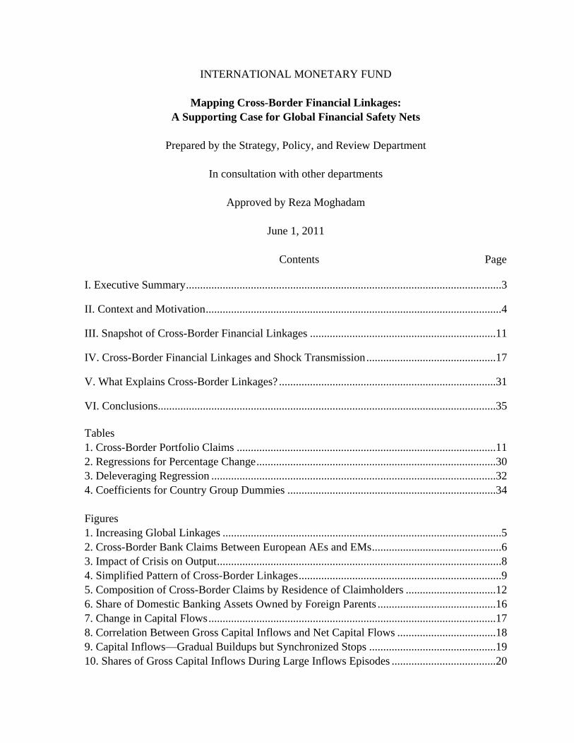
Contents Page
I. Executive Summary ................................................................................................................3
II. Context and Motivation .........................................................................................................4
III. Snapshot of Cross-Border Financial Linkages ..................................................................11
IV. Cross-Border Financial Linkages and Shock Transmission ..............................................17
V. What Explains Cross-Border Linkages? .............................................................................31
VI. Conclusions........................................................................................................................35
Tables
1. Cross-Border Portfolio Claims ............................................................................................11
2. Regressions for Percentage Change .....................................................................................30
3. Deleveraging Regression .....................................................................................................32
4. Coefficients for Country Group Dummies ..........................................................................34
Figures
1. Increasing Global Linkages ...................................................................................................5
2. Cross-Border Bank Claims Between European AEs and EMs ..............................................6
3. Impact of Crisis on Output .....................................................................................................8
4. Simplified Pattern of Cross-Border Linkages ........................................................................9
5. Composition of Cross-Border Claims by Residence of Claimholders ................................12
6. Share of Domestic Banking Assets Owned by Foreign Parents ..........................................16
7. Change in Capital Flows ......................................................................................................17
8. Correlation Between Gross Capital Inflows and Net Capital Flows ...................................18
9. Capital Inflows—Gradual Buildups but Synchronized Stops .............................................19
10. Shares of Gross Capital Inflows During Large Inflows Episodes .....................................20
2
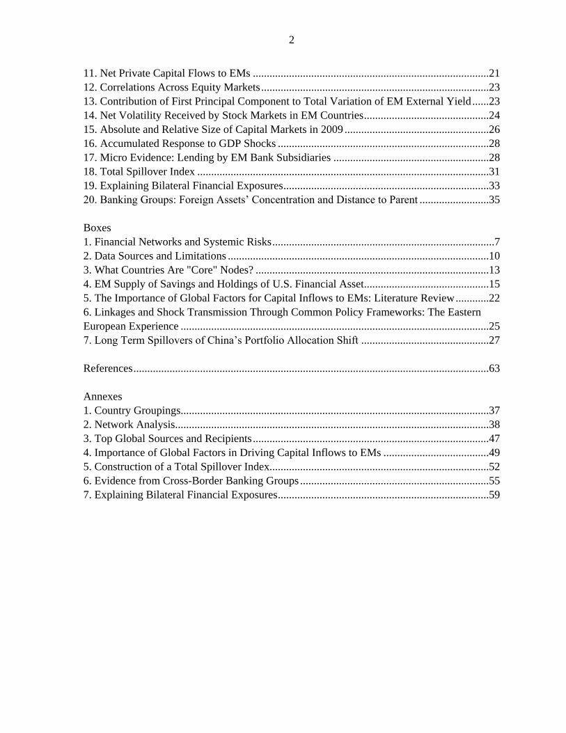
11. Net Private Capital Flows to EMs .....................................................................................21
12. Correlations Across Equity Markets ..................................................................................23
13. Contribution of First Principal Component to Total Variation of EM External Yield ......23
14. Net Volatility Received by Stock Markets in EM Countries .............................................24
15. Absolute and Relative Size of Capital Markets in 2009 ....................................................26
16. Accumulated Response to GDP Shocks ............................................................................28
17. Micro Evidence: Lending by EM Bank Subsidiaries ........................................................28
18. Total Spillover Index .........................................................................................................31
19. Explaining Bilateral Financial Exposures ..........................................................................33
20. Banking Groups: Foreign Assets‘ Concentration and Distance to Parent .........................35
Boxes
1. Financial Networks and Systemic Risks ................................................................................7
2. Data Sources and Limitations ..............................................................................................10
3. What Countries Are "Core" Nodes? ....................................................................................13
4. EM Supply of Savings and Holdings of U.S. Financial Asset.............................................15
5. The Importance of Global Factors for Capital Inflows to EMs: Literature Review ............22
6. Linkages and Shock Transmission Through Common Policy Frameworks: The Eastern
European Experience ...............................................................................................................25
7. Long Term Spillovers of China‘s Portfolio Allocation Shift ..............................................27
References ................................................................................................................................63
Annexes
1. Country Groupings...............................................................................................................37
2. Network Analysis.................................................................................................................38
3. Top Global Sources and Recipients .....................................................................................47
4. Importance of Global Factors in Driving Capital Inflows to EMs ......................................49
5. Construction of a Total Spillover Index...............................................................................52
6. Evidence from Cross-Border Banking Groups ....................................................................55
7. Explaining Bilateral Financial Exposures ............................................................................59
3
I. EXECUTIVE SUMMARY
Objectives. This paper maps cross-border financial linkages and identifies factors that drive
them, contributing to the discussion on the appropriate design of a global financial safety net
(GFSN). It builds on previous staff work and complements the findings of the companion
paper on the Analytics of Systemic Crises and the Role of Global Financial Safety Nets. This
paper notes the growing roles of financial linkages and complexity in injecting latent
instability into the global financial system, underscoring the value of a GFSN design that is
effective in forestalling the risk that a localized liquidity shock propagates through the global
financial network turning into a large-scale systemic crisis.
Mapping the linkages. Cross-border financial linkages have increased dramatically over
time and have become more complex. Yet, a few ―core‖ advanced economies (AEs),
including some financial centers, still dominate the web of linkages across asset classes and
regions, both as sources and recipients. As a result, emerging markets‘ (EMs) strongest
linkages remain with AEs, even though cross-EM linkages have increased very rapidly
during the last decade (from a low base).
Systemic instability. Increased cross-border financial linkages promote risk diversification
at the individual country level, reducing exposure to localized shocks. However, increased
interconnectedness, by facilitating transmission of shocks, also generates a network
externality that makes the global financial network more prone to systemic risk—the risk that
shocks to a ―core‖ node leads to a breakdown of the entire network. Moreover, as the extent
and complexity of cross-border financial linkages grow, investor information about specific
exposures becomes less certain, amplifying systemic risks from panic responses to shocks.
Shock transmission. The paper points out that (i) countries with shallow domestic financial
markets and concentrated exposures to a few lenders are more prone to synchronized shifts in
cross-border flows; and (ii) common factors (such as global risk aversion) increasingly drive
global financial markets and tend to intensify abruptly during periods of stress, amplifying
shock transmission. These features point to potentially large costs of systemic shocks to
―crisis bystanders‖ (countries with relatively strong fundamentals for which the likelihood of
an idiosyncratic crisis is normally low), and reinforce the case for a GFSN that is designed to
help ring-fence such countries from systemic shock contagion.
Determinants of linkages. Empirical evidence shows that geographical and historical factors
remain important determinant of cross-border linkages—in particular, stronger linkages
occur among economies closer to each other, and those that are larger, more developed, and
financially more advanced. Beyond providing general principles that could underpin the
design of a GSFN, these findings suggest that an insurance mechanism against sudden shifts
in cross-border exposures driven by aggregate or global shocks is essential to complement
local or regional risk-sharing mechanisms.
4
II. CONTEXT AND MOTIVATION1
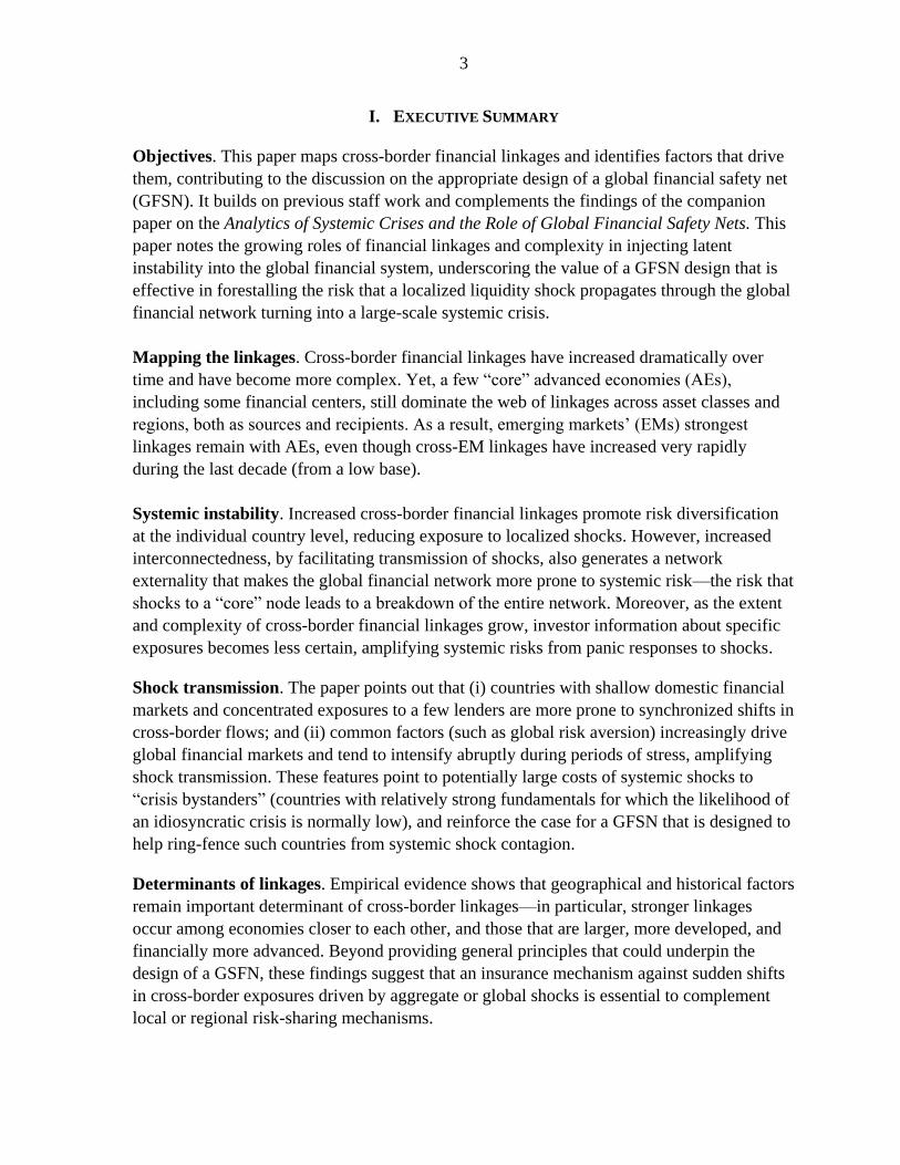
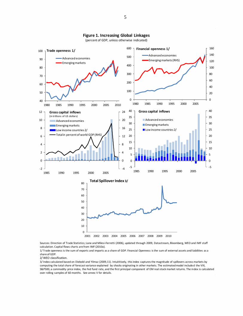
1. Global trends. Global economic linkages have intensified dramatically over the past
two decades, underpinned by an exponential rise in trade and financial flows (Figure 1).
Cross-border linkages have been dominated by financial flows among advanced economies
(AEs). However, flows to, and among, emerging markets (EMs) have also risen in
importance, both in absolute terms and in relation to the size of their economies.2 As linkages
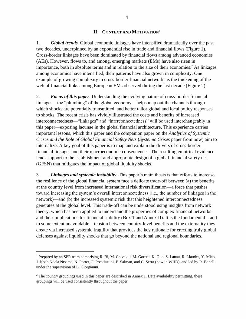
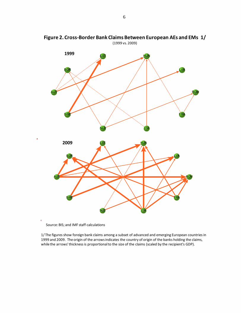
among economies have intensified, their patterns have also grown in complexity. One
example of growing complexity in cross-border financial networks is the thickening of the
web of financial links among European EMs observed during the last decade (Figure 2).
2. Focus of this paper. Understanding the evolving nature of cross-border financial
linkages—the ―plumbing‖ of the global economy—helps map out the channels through
which shocks are potentially transmitted, and better tailor global and local policy responses
to shocks. The recent crisis has vividly illustrated the costs and benefits of increased
interconnectedness—―linkages‖ and ―interconnectedness‖ will be used interchangeably in
this paper—exposing lacunae in the global financial architecture. This experience carries
important lessons, which this paper and the companion paper on the Analytics of Systemic
Crises and the Role of Global Financial Safety Nets (Systemic Crises paper from now) aim to
internalize. A key goal of this paper is to map and explain the drivers of cross-border
financial linkages and their macroeconomic consequences. The resulting empirical evidence
lends support to the establishment and appropriate design of a global financial safety net
(GFSN) that mitigates the impact of global liquidity shocks.
3. Linkages and systemic instability. This paper‘s main thesis is that efforts to increase
the resilience of the global financial system face a delicate trade-off between (a) the benefits
at the country level from increased international risk diversification—a force that pushes
toward increasing the system‘s overall interconnectedness (i.e., the number of linkages in the
network)—and (b) the increased systemic risk that this heightened interconnectedness
generates at the global level. This trade-off can be understood using insights from network
theory, which has been applied to understand the properties of complex financial networks
and their implications for financial stability (Box 1 and Annex II). It is the fundamental—and
to some extent unavoidable—tension between country-level benefits and the externality they
create via increased systemic fragility that provides the key rationale for erecting truly global
defenses against liquidity shocks that go beyond the national and regional boundaries.
1 Prepared by an SPR team comprising R. Bi, M. Chivakul, M. Goretti, K. Guo, S. Lanau, R. Llaudes, Y. Miao,
J. Noah Ndela Ntsama, N. Porter, F. Presciuttini, F. Salman, and C. Serra (now in WHD), and led by R. Benelli
under the supervision of L. Giorgianni.
2 The country groupings used in this paper are described in Annex 1. Data availability permitting, these
groupings will be used consistently throughout the paper.
5
40
50
60
70
80
90
100
1980 1985 1990 1995 2000 2005 2010
Advanced economies
Emerging markets
Trade openness 1/
0
20
40
60
80
100
120
140
160
0
100
200
300
400
500
600
1980 1985 1990 1995 2000 2005
Advanced economies
Emerging markets (RHS)
Financial openness 1/
Figure 1. Increasing Global Linkages(percent of GDP, unless otherwise indicated)
Sources: Direction of Trade Statistics; Lane and Milesi-Ferretti (2006), updated through 2009, Datastream, Bloomberg, WEO and IMF staff calculation. Capital flows charts are from IMF (2010a).
1/ Trade openness is the sum of exports and imports as a share of GDP. Financial Openness is the sum of external assets and l iabiliites as a share of GDP.2/ WEO classification.3/ Index calculated based on Diebold and Yilmaz (2009,11). Intuititively, this index captures the magnitude of spillovers across markets by computing the total share of forecast variance explained by shocks originating in other markets. The estimated model included the VIX, S&P500, a commodity price index, the Fed fund rate, and the first principal component of EM real stock market returns. The index is calculated over rolling samples of 60 months. See annex V for details.
0
10
20
30
40
50
60
70
80
2001 2002 2003 2004 2005 2006 2007 2008 2009 2010
Total Spillover Index 3/
-4
0
4
8
12
16
20
24
-2
0
2
4
6
8
10
12
1985 1990 1995 2000 2005
Advanced economies
Emerging markets
Low income countries 2/
Total in percent of world GDP (RHS)
Gross capital inflows(in trillions of US dollars)
-5
0
5
10
15
20
25
30
35
40
-5
0
5
10
15
20
25
30
35
40
1985 1990 1995 2000 2005
Advanced economies
Emerging markets
Low income countries 2/
Gross capital inflows
6
1999
2009
Figure 2. Cross-Border Bank Claims Between European AEs and EMs 1/(1999 vs. 2009)
Source: BIS; and IMF staff calculations
1/ The figures show foreign bank claims among a subset of advanced and emerging European countries in 1999 and 2009. The origin of the arrows indicates the country of origin of the banks holding the claims, while the arrows' thickness is proportional to the size of the claims (scaled by the recipient's GDP).
7
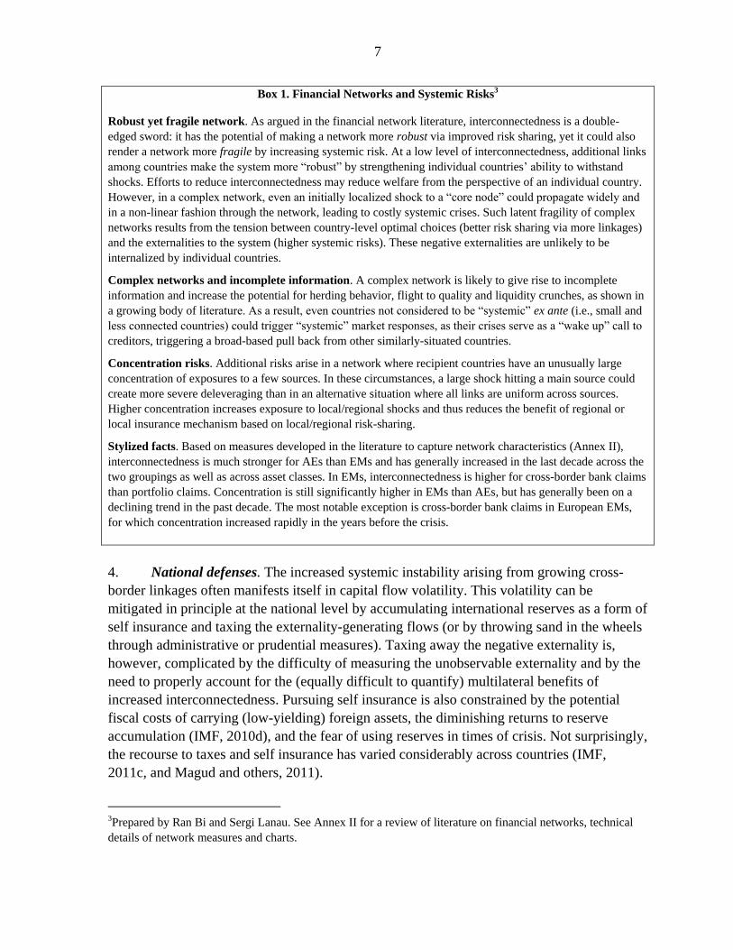
Box 1. Financial Networks and Systemic Risks3
Robust yet fragile network. As argued in the financial network literature, interconnectedness is a double-
edged sword: it has the potential of making a network more robust via improved risk sharing, yet it could also
render a network more fragile by increasing systemic risk. At a low level of interconnectedness, additional links
among countries make the system more ―robust‖ by strengthening individual countries‘ ability to withstand
shocks. Efforts to reduce interconnectedness may reduce welfare from the perspective of an individual country.
However, in a complex network, even an initially localized shock to a ―core node‖ could propagate widely and
in a non-linear fashion through the network, leading to costly systemic crises. Such latent fragility of complex
networks results from the tension between country-level optimal choices (better risk sharing via more linkages)
and the externalities to the system (higher systemic risks). These negative externalities are unlikely to be
internalized by individual countries.
Complex networks and incomplete information. A complex network is likely to give rise to incomplete
information and increase the potential for herding behavior, flight to quality and liquidity crunches, as shown in
a growing body of literature. As a result, even countries not considered to be ―systemic‖ ex ante (i.e., small and
less connected countries) could trigger ―systemic‖ market responses, as their crises serve as a ―wake up‖ call to
creditors, triggering a broad-based pull back from other similarly-situated countries.
Concentration risks. Additional risks arise in a network where recipient countries have an unusually large
concentration of exposures to a few sources. In these circumstances, a large shock hitting a main source could
create more severe deleveraging than in an alternative situation where all links are uniform across sources.
Higher concentration increases exposure to local/regional shocks and thus reduces the benefit of regional or
local insurance mechanism based on local/regional risk-sharing.
Stylized facts. Based on measures developed in the literature to capture network characteristics (Annex II),
interconnectedness is much stronger for AEs than EMs and has generally increased in the last decade across the
two groupings as well as across asset classes. In EMs, interconnectedness is higher for cross-border bank claims
than portfolio claims. Concentration is still significantly higher in EMs than AEs, but has generally been on a
declining trend in the past decade. The most notable exception is cross-border bank claims in European EMs,
for which concentration increased rapidly in the years before the crisis.
4. National defenses. The increased systemic instability arising from growing cross-
border linkages often manifests itself in capital flow volatility. This volatility can be
mitigated in principle at the national level by accumulating international reserves as a form of
self insurance and taxing the externality-generating flows (or by throwing sand in the wheels
through administrative or prudential measures). Taxing away the negative externality is,
however, complicated by the difficulty of measuring the unobservable externality and by the
need to properly account for the (equally difficult to quantify) multilateral benefits of
increased interconnectedness. Pursuing self insurance is also constrained by the potential
fiscal costs of carrying (low-yielding) foreign assets, the diminishing returns to reserve
accumulation (IMF, 2010d), and the fear of using reserves in times of crisis. Not surprisingly,
the recourse to taxes and self insurance has varied considerably across countries (IMF,
2011c, and Magud and others, 2011).
3Prepared by Ran Bi and Sergi Lanau. See Annex II for a review of literature on financial networks, technical
details of network measures and charts.
8
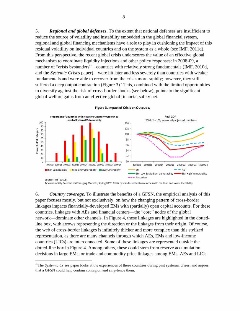
5. Regional and global defenses. To the extent that national defenses are insufficient to
reduce the source of volatility and instability embedded in the global financial system,
regional and global financing mechanisms have a role to play in cushioning the impact of this
residual volatility on individual countries and on the system as a whole (see IMF, 2011d).
From this perspective, the recent global crisis underscores the value of an effective global
mechanism to coordinate liquidity injections and other policy responses: in 2008-09, a
number of ―crisis bystanders‖—countries with relatively strong fundamentals (IMF, 2010d,
and the Systemic Crises paper)—were hit later and less severely than countries with weaker
fundamentals and were able to recover from the crisis more rapidly; however, they still
suffered a deep output contraction (Figure 3).4 This, combined with the limited opportunities
to diversify against the risk of cross-border shocks (see below), points to the significant
global welfare gains from an effective global financial safety net.
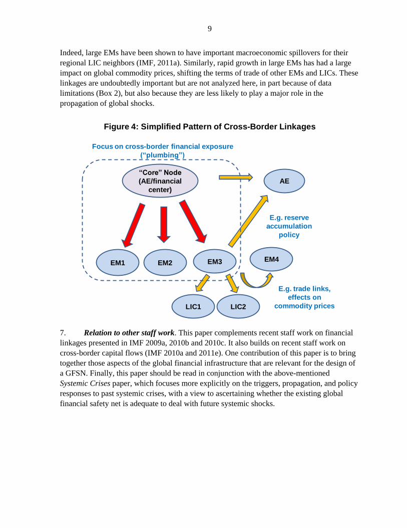
6. Country coverage. To illustrate the benefits of a GFSN, the empirical analysis of this
paper focuses mostly, but not exclusively, on how the changing pattern of cross-border
linkages impacts financially-developed EMs with (partially) open capital accounts. For these
countries, linkages with AEs and financial centers—the ―core‖ nodes of the global
network—dominate other channels. In Figure 4, these linkages are highlighted in the dotted-
line box, with arrows representing the direction or the linkages from their origin. Of course,
the web of cross-border linkages is infinitely thicker and more complex than this stylized
representation, as there are many channels through which AEs, EMs and low-income
countries (LICs) are interconnected. Some of these linkages are represented outside the
dotted-line box in Figure 4. Among others, these could stem from reserve accumulation
decisions in large EMs, or trade and commodity price linkages among EMs, AEs and LICs.
4 The Systemic Crises paper looks at the experiences of these countries during past systemic crises, and argues
that a GFSN could help contain contagion and ring-fence them.
90
92
94
96
98
100
102
104
2008Q2 2008Q3 2008Q4 2009Q1 2009Q2 2009Q3 2009Q4
Real GDP(2008q2 = 100, seasonally adjusted, medians)
EM AE
EM: Low & Medium Vulnerability EM: High Vulnerability
Past crises
0
10
20
30
40
50
60
70
80
90
100
2007Q4 2008Q1 2008Q2 2008Q3 2008Q4 2009Q1 2009Q2 2009Q3 2009q4
Pe
rce
nt o
f VE
cate
gory
Proportion of Countries with Negative Quarterly Growth by Level of External Vulnerability
High vulnerability Medium vulnerability Low vulnerability
Figure 3. Impact of Crisis on Output 1/
Source: IMF (2010d).1/ Vulnerability Exercise for Emerging Markets, Spring 2007. Crisis bystanders refer to countries with medium and low vulnerability.
9
Indeed, large EMs have been shown to have important macroeconomic spillovers for their
regional LIC neighbors (IMF, 2011a). Similarly, rapid growth in large EMs has had a large
impact on global commodity prices, shifting the terms of trade of other EMs and LICs. These
linkages are undoubtedly important but are not analyzed here, in part because of data
limitations (Box 2), but also because they are less likely to play a major role in the
propagation of global shocks.
7. Relation to other staff work. This paper complements recent staff work on financial
linkages presented in IMF 2009a, 2010b and 2010c. It also builds on recent staff work on
cross-border capital flows (IMF 2010a and 2011e). One contribution of this paper is to bring
together those aspects of the global financial infrastructure that are relevant for the design of
a GFSN. Finally, this paper should be read in conjunction with the above-mentioned
Systemic Crises paper, which focuses more explicitly on the triggers, propagation, and policy
responses to past systemic crises, with a view to ascertaining whether the existing global
financial safety net is adequate to deal with future systemic shocks.
Figure 4: Simplified Pattern of Cross-Border Linkages
“Core” Node
(AE/financial
center)
EM1 EM2 EM3 EM4
E.g. reserve
accumulation
policy
E.g. trade links,
effects on
commodity prices
Focus on cross-border financial exposure
(“plumbing”)
LIC1 LIC2
AE
10
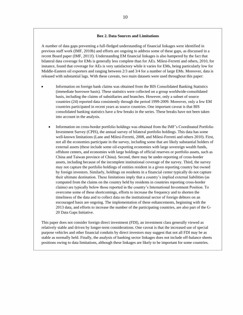
Box 2. Data Sources and Limitations
A number of data gaps preventing a full-fledged understanding of financial linkages were identified in
previous staff work (IMF, 2010b) and efforts are ongoing to address some of these gaps, as discussed in a
recent Board paper (IMF, 2011f). Understanding EM financial linkages is also hampered by the fact that
bilateral data coverage for EMs is generally less complete than for AEs. Milesi-Ferretti and others, 2010, for
instance, found that coverage for AEs is very satisfactory while it varies for EMs, being particularly low for
Middle-Eastern oil exporters and ranging between 2/3 and 3/4 for a number of large EMs. Moreover, data is
released with substantial lags. With these caveats, two main datasets were used throughout this paper:
Information on foreign bank claims was obtained from the BIS Consolidated Banking Statistics
(immediate borrower basis). These statistics were collected on a group worldwide-consolidated
basis, including the claims of subsidiaries and branches. However, only a subset of source
countries (24) reported data consistently through the period 1999-2009. Moreover, only a few EM
countries participated in recent years as source countries. One important caveat is that BIS
consolidated banking statistics have a few breaks in the series. These breaks have not been taken
into account in the analysis.
Information on cross-border portfolio holdings was obtained from the IMF‘s Coordinated Portfolio
Investment Survey (CPIS), the annual survey of bilateral portfolio holdings. This data has some
well-known limitations (Lane and Milesi-Ferretti, 2008, and Milesi-Ferretti and others 2010). First,
not all the economies participate in the survey, including some that are likely substantial holders of
external assets (these include some oil-exporting economies with large sovereign wealth funds,
offshore centers, and economies with large holdings of official reserves or portfolio assets, such as
China and Taiwan province of China). Second, there may be under-reporting of cross-border
assets, including because of the incomplete institutional coverage of the survey. Third, the survey
may not capture the portfolio holdings of entities resident in a given reporting country but owned
by foreign investors. Similarly, holdings on residents in a financial center typically do not capture
their ultimate destination. These limitations imply that a country‘s implied external liabilities (as
computed from the claims on the country held by residents in countries reporting cross-border
claims) are typically below those reported in the country‘s International Investment Position. To
overcome some of these shortcomings, efforts to increase the frequency and to shorten the
timeliness of the data and to collect data on the institutional sector of foreign debtors on an
encouraged basis are ongoing. The implementation of these enhancements, beginning with the
2013 data, and efforts to increase the number of the participating countries, are also part of the G-
20 Data Gaps Initiative.
This paper does not consider foreign direct investment (FDI), an investment class generally viewed as
relatively stable and driven by longer-term considerations. One caveat is that the increased use of special
purpose vehicles and other financial conduits by direct investors may suggest that not all FDI may be as
stable as normally held. Finally, the analysis of banking sector linkages does not include off-balance sheets
positions owing to data limitations, although these linkages are likely to be important for some countries.
11
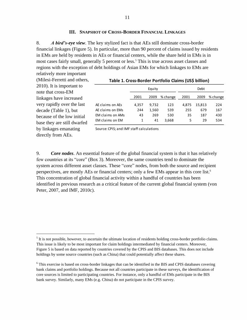
2001 2009 % change 2001 2009 % change
AE claims on AEs 4,357 9,732 123 4,875 15,813 224
AE claims on EMs 244 1,560 539 255 679 167
EM claims on AMs 43 269 530 35 187 430
EM claims on EM 1 41 3,668 5 29 534
Source: CPIS; and IMF staff calculations
Equity Debt
Table 1. Cross-Border Portfolio Claims (US$ billion)
III. SNAPSHOT OF CROSS-BORDER FINANCIAL LINKAGES
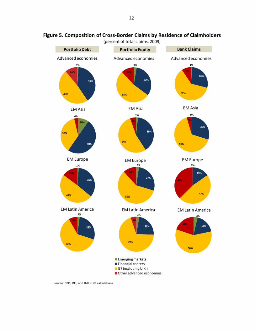
8. A bird’s-eye view. The key stylized fact is that AEs still dominate cross-border
financial linkages (Figure 5). In particular, more than 90 percent of claims issued by residents
in EMs are held by residents in AEs or financial centers, while the share held in EMs is in
most cases fairly small, generally 5 percent or less.5 This is true across asset classes and
regions with the exception of debt holdings of Asian EMs for which linkages to EMs are
relatively more important
(Milesi-Ferretti and others,
2010). It is important to
note that cross-EM
linkages have increased
very rapidly over the last
decade (Table 1), but
because of the low initial
base they are still dwarfed
by linkages emanating
directly from AEs.
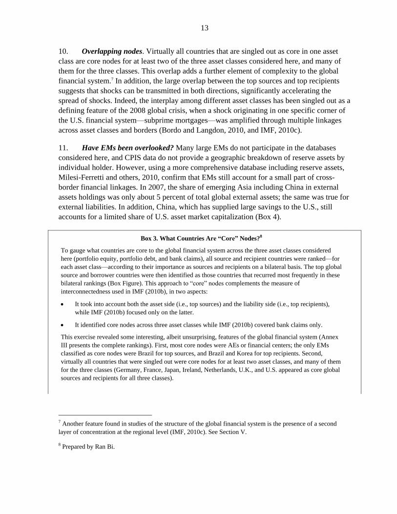
9. Core nodes. An essential feature of the global financial system is that it has relatively
few countries at its ―core‖ (Box 3). Moreover, the same countries tend to dominate the
system across different asset classes. These ―core‖ nodes, from both the source and recipient
perspectives, are mostly AEs or financial centers; only a few EMs appear in this core list.6
This concentration of global financial activity within a handful of countries has been
identified in previous research as a critical feature of the current global financial system (von
Peter, 2007, and IMF, 2010c).
5 It is not possible, however, to ascertain the ultimate location of residents holding cross-border portfolio claims.
This issue is likely to be most important for claim holdings intermediated by financial centers. Moreover,
Figure 5 is based on data reported by countries covered by the CPIS and BIS databases. This does not include
holdings by some source countries (such as China) that could potentially affect these shares.
6 This exercise is based on cross-border linkages that can be identified in the BIS and CPIS databases covering
bank claims and portfolio holdings. Because not all countries participate in these surveys, the identification of
core sources is limited to participating countries. For instance, only a handful of EMs participate in the BIS
bank survey. Similarly, many EMs (e.g. China) do not participate in the CPIS survey.
12
1%
39%
49%
11%
Advanced economies
10%
50%
36%
4%
EM Asia
1%
35%
49%
15%
EM Europe
2%
28%
62%
8%
EM Latin America
3%
32%
53%
12%
Advanced economies
2%
39%
54%
5%
EM Asia
2%
27%
59%
12%
EM Europe
3%
23%
69%
5%
EM Latin America
Emerging marketsFinancial centersG7 (excluding U.K.)Other advanced economies
1%
28%
62%
9%
Advanced economies
0%
30%
65%
5%
EM Asia
0%
15%
47%
38%
EM Europe
4%
18%
58%
20%
EM Latin America
Portfolio Debt Portfolio Equity Bank Claims
Figure 5. Composition of Cross-Border Claims by Residence of Claimholders (percent of total claims, 2009)
Source: CPIS; BIS; and IMF staff calculations
13
10. Overlapping nodes. Virtually all countries that are singled out as core in one asset
class are core nodes for at least two of the three asset classes considered here, and many of
them for the three classes. This overlap adds a further element of complexity to the global
financial system.7 In addition, the large overlap between the top sources and top recipients
suggests that shocks can be transmitted in both directions, significantly accelerating the
spread of shocks. Indeed, the interplay among different asset classes has been singled out as a
defining feature of the 2008 global crisis, when a shock originating in one specific corner of
the U.S. financial system—subprime mortgages—was amplified through multiple linkages
across asset classes and borders (Bordo and Langdon, 2010, and IMF, 2010c).
11. Have EMs been overlooked? Many large EMs do not participate in the databases
considered here, and CPIS data do not provide a geographic breakdown of reserve assets by
individual holder. However, using a more comprehensive database including reserve assets,
Milesi-Ferretti and others, 2010, confirm that EMs still account for a small part of cross-
border financial linkages. In 2007, the share of emerging Asia including China in external
assets holdings was only about 5 percent of total global external assets; the same was true for
external liabilities. In addition, China, which has supplied large savings to the U.S., still
accounts for a limited share of U.S. asset market capitalization (Box 4).
7 Another feature found in studies of the structure of the global financial system is the presence of a second
layer of concentration at the regional level (IMF, 2010c). See Section V.
8 Prepared by Ran Bi.
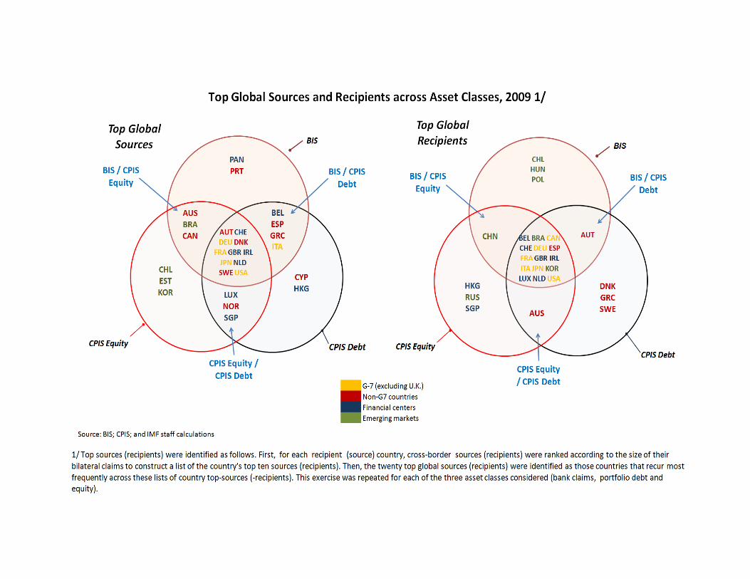
Box 3. What Countries Are “Core” Nodes?
8
To gauge what countries are core to the global financial system across the three asset classes considered
here (portfolio equity, portfolio debt, and bank claims), all source and recipient countries were ranked—for
each asset class—according to their importance as sources and recipients on a bilateral basis. The top global
source and borrower countries were then identified as those countries that recurred most frequently in these
bilateral rankings (Box Figure). This approach to ―core‖ nodes complements the measure of
interconnectedness used in IMF (2010b), in two aspects:
It took into account both the asset side (i.e., top sources) and the liability side (i.e., top recipients),
while IMF (2010b) focused only on the latter.
It identified core nodes across three asset classes while IMF (2010b) covered bank claims only.
This exercise revealed some interesting, albeit unsurprising, features of the global financial system (Annex
III presents the complete rankings). First, most core nodes were AEs or financial centers; the only EMs
classified as core nodes were Brazil for top sources, and Brazil and Korea for top recipients. Second,
virtually all countries that were singled out were core nodes for at least two asset classes, and many of them
for the three classes (Germany, France, Japan, Ireland, Netherlands, U.K., and U.S. appeared as core global
sources and recipients for all three classes).
15
90%
6%
3%
US residentsAdvanced marketsFinancial centersChinaOther emerging marketsMiddle Easter oil producersOthers
Holders of U.S. Equities in 2009
73%
11%
5%
5%
4%
US residentsAdvanced marketsFinancial centersChinaOther emerging marketsMiddle Easter oil producersOthers
Holders of U.S. Debt in 2009
Source: TIC and IMF staff calculations.
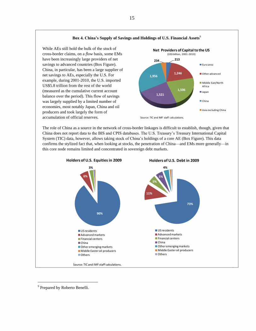
Box 4. China’s Supply of Savings and Holdings of U.S. Financial Assets9
While AEs still hold the bulk of the stock of
cross-border claims, on a flow basis, some EMs
have been increasingly large providers of net
savings to advanced countries (Box Figure).
China, in particular, has been a large supplier of
net savings to AEs, especially the U.S. For
example, during 2001-2010, the U.S. imported
US$5.8 trillion from the rest of the world
(measured as the cumulative current account
balance over the period). This flow of savings
was largely supplied by a limited number of
economies, most notably Japan, China and oil
producers and took largely the form of
accumulation of official reserves.
The role of China as a source in the network of cross-border linkages is difficult to establish, though, given that
China does not report data to the BIS and CPIS databases. The U.S. Treasury‘s Treasury International Capital
System (TIC) data, however, allows taking stock of China‘s holdings of a core AE (Box Figure). This data
confirms the stylized fact that, when looking at stocks, the penetration of China—and EMs more generally—in
this core node remains limited and concentrated in sovereign debt markets.
9 Prepared by Roberto Benelli.
213
1,246
1,506
1,521
1,956
234Euro area
Other advanced
Middle East/North Africa
Japan
China
Asia excluding China
Net Providers of Capital to the US(US$ billion, 2001-2010)
Source: TIC and IMF staff calculations.
16
Sources: Bankscope and IMF staff calculations. See annex VI for details.
0
10
20
30
40
1995 1997 1999 2001 2003 2005 2007 2009
EM (Asia)
EM parents
Other AMs parents
Financial center parents
G7 (excluding U.K.) parents
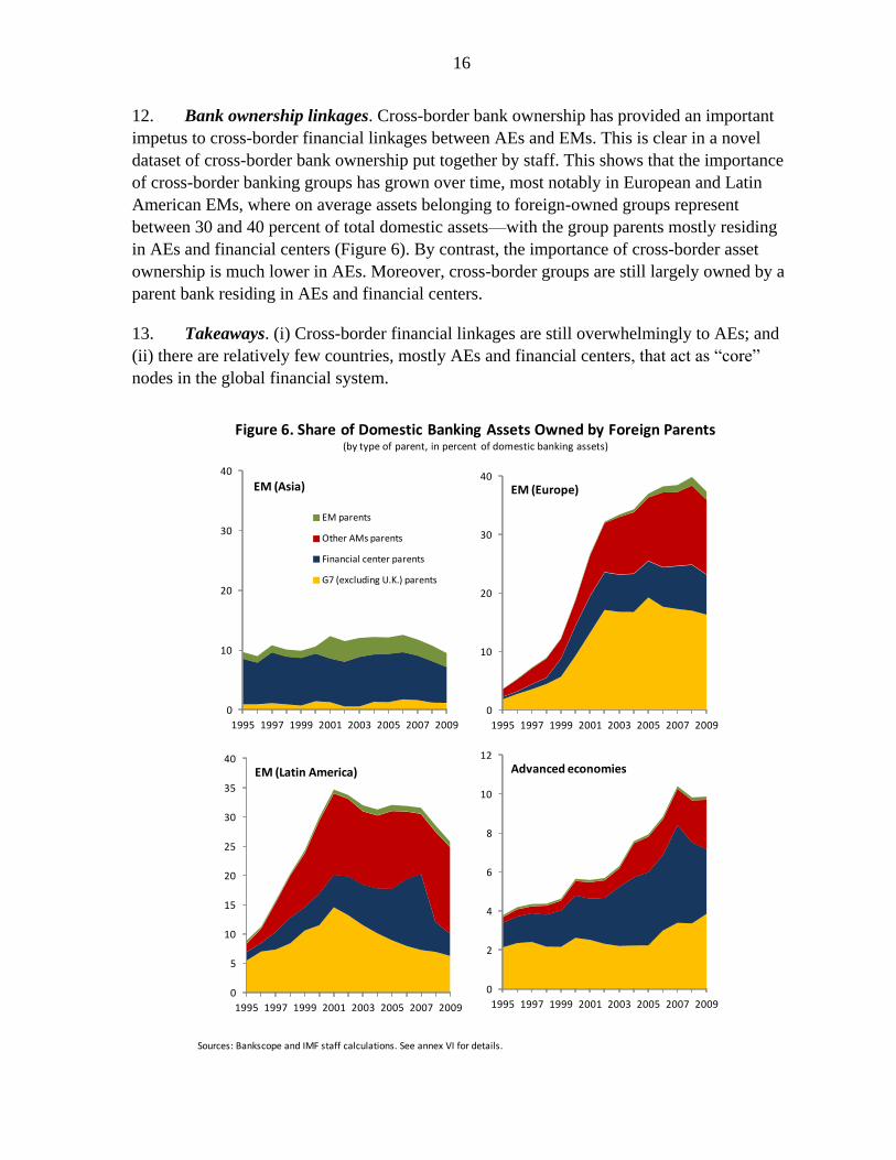
Figure 6. Share of Domestic Banking Assets Owned by Foreign Parents(by type of parent, in percent of domestic banking assets)
0
10
20
30
40
1995 1997 1999 2001 2003 2005 2007 2009
EM (Europe)
0
5
10
15
20
25
30
35
40
1995 1997 1999 2001 2003 2005 2007 2009
EM (Latin America)
0
2
4
6
8
10
12
1995 1997 1999 2001 2003 2005 2007 2009
Advanced economies
12. Bank ownership linkages. Cross-border bank ownership has provided an important
impetus to cross-border financial linkages between AEs and EMs. This is clear in a novel
dataset of cross-border bank ownership put together by staff. This shows that the importance
of cross-border banking groups has grown over time, most notably in European and Latin
American EMs, where on average assets belonging to foreign-owned groups represent
between 30 and 40 percent of total domestic assets—with the group parents mostly residing
in AEs and financial centers (Figure 6). By contrast, the importance of cross-border asset
ownership is much lower in AEs. Moreover, cross-border groups are still largely owned by a
parent bank residing in AEs and financial centers.
13. Takeaways. (i) Cross-border financial linkages are still overwhelmingly to AEs; and
(ii) there are relatively few countries, mostly AEs and financial centers, that act as ―core‖
nodes in the global financial system.
17
IV. CROSS-BORDER FINANCIAL LINKAGES AND SHOCK TRANSMISSION
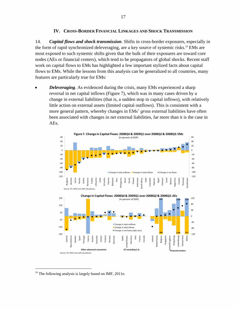
14. Capital flows and shock transmission. Shifts in cross-border exposures, especially in
the form of rapid synchronized deleveraging, are a key source of systemic risks.10 EMs are
most exposed to such systemic shifts given that the bulk of their exposures are toward core
nodes (AEs or financial centers), which tend to be propagators of global shocks. Recent staff
work on capital flows to EMs has highlighted a few important stylized facts about capital
flows to EMs. While the lessons from this analysis can be generalized to all countries, many
features are particularly true for EMs:
Deleveraging. As evidenced during the crisis, many EMs experienced a sharp
reversal in net capital inflows (Figure 7), which was in many cases driven by a
change in external liabilities (that is, a sudden stop in capital inflows), with relatively
little action on external assets (limited capital outflows). This is consistent with a
more general pattern, whereby changes in EMs‘ gross external liabilities have often
been associated with changes in net external liabilities, far more than it is the case in
AEs.
10 The following analysis is largely based on IMF, 2011e.
-120
-100
-80
-60
-40
-20
0
20
40
60
-120
-100
-80
-60
-40
-20
0
20
40
60
Bu
lga
ria
Ukr
ain
e
Latv
ia
Ru
ssia
Serb
ia
Ro
ma
nia
Turk
ey
Lith
uan
ia
Ch
ile
Sri L
anka
Esto
nia
Mal
aysi
a
Per
u
Ph
ilip
pin
es
Bra
zil
Ko
rea
Po
lan
d
Ind
on
esia
Sou
th A
fric
a
Ind
ia
Co
lom
bia
Paki
stan
Egyp
t
Vie
tnam
Isra
el
Mex
ico
Arg
en
tin
a
Cro
ati
a
Thai
lan
d
Kaz
akh
stan
Change in total outflows Change in total Inflows Change in net flows
Figure 7. Change in Capital Flows: 2008Q4 & 2009Q1 over 2008Q2 & 2008Q3: EMs(In percent of GDP)
Source: IFS, WEO and staff calculations.
-120
-80
-40
0
40
80
120
-250
-150
-50
50
150
250
Ice
lan
d
New
Zea
lan
d
Swed
en
Spa
in
Po
rtu
gal
Cyp
rus
Au
stri
a
Au
stra
lia
Gre
ece
Fin
lan
d
No
rwa
y
Den
mar
k
Jap
an
Un
ited
Sta
tes
Ger
ma
ny
Ita
ly
Fran
ce
Ca
na
da
Irel
and
Net
her
lan
ds
Bel
giu
m
Sin
gap
ore
Un
ited
Kin
gdo
m
Ho
ng
Ko
ng
Luxe
mb
ou
rg
Swit
zerl
an
d
Ma
lta
Change in total outflows
Change in total Inflows
Change in net flows (right axis)
Change in Capital Flows: 2008Q4 & 2009Q1 over 2008Q2 & 2008Q3: AEs(In percent of GDP)
Source: IFS, WEO and staff calculations.
Other advanced economies G7 excluding U.K. Financial centers
1246
1190
810
727
310
306
18
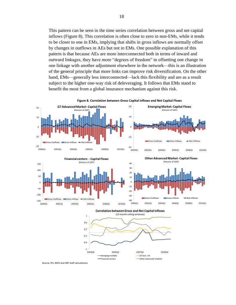
This pattern can be seen in the time series correlation between gross and net capital
inflows (Figure 8). This correlation is often close to zero in non-EMs, while it tends
to be closer to one in EMs, implying that shifts in gross inflows are normally offset
by changes in outflows in AEs but not in EMs. One possible explanation of this
pattern is that because AEs are more interconnected both in terms of inward and
outward linkages, they have more ―degrees of freedom‖ in offsetting one change in
one linkage with another adjustment elsewhere in the network—this is an illustration
of the general principle that more links can improve risk diversification. On the other
hand, EMs—generally less interconnected—lack this flexibility and are as a result
subject to the higher one-way risk of deleveraging. It follows that EMs stand to
benefit the most from a global insurance mechanism against this risk.
-1
-0.6
-0.2
0.2
0.6
1
2003Q4 2005Q4 2007Q4 2009Q4
Emerging markets G7 excl. UK
Financial centers Other advanced markets
Correlation between Gross and Net Capital Inflows(12-month rolling windows)
-20
-10
0
10
20
2000Q1 2002Q1 2004Q1 2006Q1 2008Q1 2010Q1
Gross Outflows Gross Inflows Net Intflows
Emerging Market- Capital Flows(Percent of GDP)
-20
-10
0
10
20
2000Q1 2002Q1 2004Q1 2006Q1 2008Q1 2010Q1
Gross Outflows Gross Inflows Net Intflows
G7 Advanced Market- Capital Flows(Percent of GDP)
-150
-100
-50
0
50
100
150
2000Q1 2002Q1 2004Q1 2006Q1 2008Q1 2010Q1
Gross Outflows Gross Inflows Net Intflows
Financial centers - Capital Flows(Percent of GDP)
-40
-30
-20
-10
0
10
20
30
40
2000Q1 2002Q1 2004Q1 2006Q1 2008Q1 2010Q1
Gross Outflows Gross Inflows Net Intflows
Other Advanced Market- Capital Flows(Percent of GDP)
Source: IFS, WEO and IMF staff calculations.
Figure 8. Correlation between Gross Capital inflows and Net Capital Flows
19
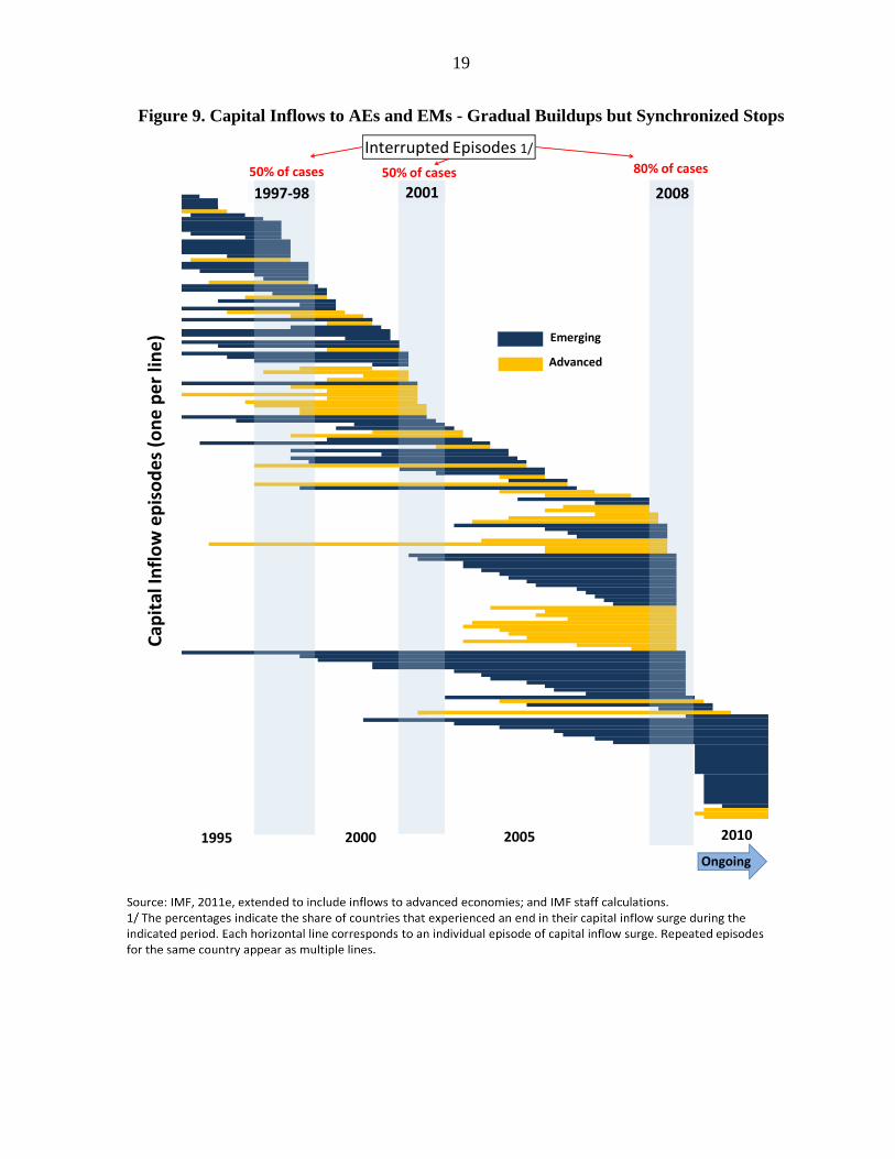
Figure 9. Capital Inflows to AEs and EMs - Gradual Buildups but Synchronized Stops
1997-98 2001 2008
2010200520001995
Interrupted Episodes 1/
50% of cases 50% of cases 80% of cases
Ongoing
Cap
ital
Infl
ow
ep
iso
de
s (o
ne
pe
r lin
e) Emerging
Advanced
Source: IMF, 2011e, extended to include inflows to advanced economies; and IMF staff calculations.
20
Synchronization. Shifts in cross-border exposures can be highly synchronized,
especially at times of stress. Episodes of capital inflow surges normally start at
different times, likely a reflection of country-specific circumstances and pull factors,11
but often end together within a narrow time period (Figure 9), as seen for example
during the sudden stop episodes of 1997−98 and 2008−09. This suggests that behind
these reversals are exogenous factors, such as sudden shocks to global risk appetite.
This feature also explains why an insurance mechanism against sudden shifts in
cross-border exposures driven by aggregate or global shocks cannot be based
exclusively on local or regional risk-sharing mechanisms (Holmström and Tirole,
1998, and Levy-Yeyati, 2010). The evidence discussed in Section V that there remain
strong geographical patterns in cross-border networks further reinforces the case for a
global insurance mechanism.
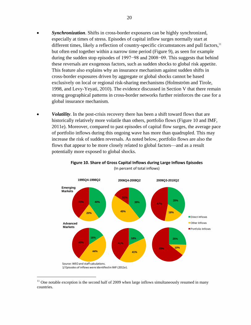
Volatility. In the post-crisis recovery there has been a shift toward flows that are
historically relatively more volatile than others, portfolio flows (Figure 10 and IMF,
2011e). Moreover, compared to past episodes of capital flow surges, the average pace
of portfolio inflows during this ongoing wave has more than quadrupled. This may
increase the risk of sudden reversals. As noted below, portfolio flows are also the
flows that appear to be more closely related to global factors—and as a result
potentially more exposed to global shocks.
Figure 10. Share of Gross Capital Inflows during Large Inflows Episodes
(In percent of total inflows)
11 One notable exception is the second half of 2009 when large inflows simultaneously resumed in many
countries.
40%
20%
40%35%
18%
47%39%
45%
16%
16%
44%
40%
18%
41%
41%
25%
10%65%
Direct Inf lows
Other Inf lows
Portfolio Inf lows
2006Q4-2008Q21995Q4-1998Q2 2009Q3-2010Q2
Emerging Markets
Advanced Markets
Source: WEO and staff calculations.1/ Episodes of inflows were identified in IMF (2011e).
21
-1
0
1
2
3
4
5
-1
0
1
2
3
4
5
Before During After
Bank and other private flows
Portfolio debt flows
Portfolio equity flows
Foreign direct investment
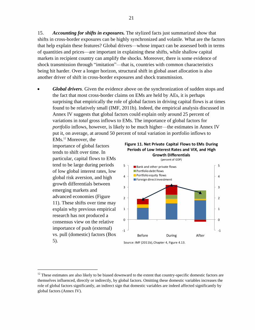
Figure 11. Net Private Capital Flows to EMs During Periods of Low Interest Rates and VIX, and High
Growth Differentials(percent of GDP)
Source: IMF (2011b), Chapter 4, Figure 4.13.
15. Accounting for shifts in exposures. The stylized facts just summarized show that
shifts in cross-border exposures can be highly synchronized and volatile. What are the factors
that help explain these features? Global drivers—whose impact can be assessed both in terms
of quantities and prices—are important in explaining these shifts, while shallow capital
markets in recipient country can amplify the shocks. Moreover, there is some evidence of
shock transmission through ―imitation‖—that is, countries with common characteristics
being hit harder. Over a longer horizon, structural shift in global asset allocation is also
another driver of shift in cross-border exposures and shock transmission.
Global drivers. Given the evidence above on the synchronization of sudden stops and
the fact that most cross-border claims on EMs are held by AEs, it is perhaps
surprising that empirically the role of global factors in driving capital flows is at times
found to be relatively small (IMF, 2011b). Indeed, the empirical analysis discussed in
Annex IV suggests that global factors could explain only around 25 percent of
variations in total gross inflows to EMs. The importance of global factors for
portfolio inflows, however, is likely to be much higher—the estimates in Annex IV
put it, on average, at around 50 percent of total variation in portfolio inflows to
EMs.12 Moreover, the
importance of global factors
tends to shift over time. In
particular, capital flows to EMs
tend to be large during periods
of low global interest rates, low
global risk aversion, and high
growth differentials between
emerging markets and
advanced economies (Figure
11). These shifts over time may
explain why previous empirical
research has not produced a
consensus view on the relative
importance of push (external)
vs. pull (domestic) factors (Box
5).
12 These estimates are also likely to be biased downward to the extent that country-specific domestic factors are
themselves influenced, directly or indirectly, by global factors. Omitting these domestic variables increases the
role of global factors significantly, an indirect sign that domestic variables are indeed affected significantly by
global factors (Annex IV).
22
Box 5. The Importance of Global Factors for Capital Inflows to EMs: Literature Review13
There seems to be lack of consensus in the empirical literature on the quantitative importance of global
factors as drivers of capital flows to EMs. This box briefly summarizes some findings at the opposite
extremes of this literature.
The first generation of empirical literature, inspired by the surge of capital flows into EMs in the
1990s, favored the push view. Summarizing the early literature, Fernandez-Arias and Montiel, 1996,
concluded that falling U.S. interest rates played a dominant role in driving capital flows to developing
countries. Fernandez-Arias, 1996, further estimated that the fall in international interest rates explained
86 percent of the increase in portfolio flows in 13 middle income countries between 1989 and 1994.
Chuhan and others, 1993, found that global factors such as the fall in U.S. interest rates and the
slowdown in the U.S. economy explained about half of the increase in equity and bond flows to nine
Latin American countries. For Asian countries, they estimated that external factors accounted for about
one-third of portfolio flows into the region.
More recent literature, however, has suggested that pull factors and country fundamentals are
relatively more important. Using a variance decomposition approach, Mody and others, 2001,
concluded that domestic pull factors dominated push factors in explaining a large portion of the
forecast variance. More recently, IMF, 2011b, showed that global factors explained 20 percent of the
variation in net capital flows into EMs.
Despite these differences in view about the importance of global factors for total capital flows into
EMs, there has been less divergence in the literature that push factors have played a more significant
role in explaining certain type of flows, e.g., portfolio bond flows. Summarizing two strands of
research carried out at the Bank of England, Ferrucci and others, 2004, noted that push factors, and in
particular U.S. short-term interest rates, explained two thirds of the compression in EM bond spreads.
The contribution of push factors was found to be less significant for banking flows than for other asset
classes but almost as important as pull factors.
The lack of a consensus view on the relative importance of push and pull factors may simply reflect the
fact that their respective roles vary substantially over time and across countries, a point echoed by
Lane, 2009.
13 Prepared by Yanliang Miao.
23
0.0
0.1
0.2
0.3
0.4
0.5
0.6
0.7
0.8
0.9
1.0
0.0
0.1
0.2
0.3
0.4
0.5
0.6
0.7
0.8
0.9
1.0
2000 2002 2004 2006 2008 2010
Emerging Asia & Latam
Latam & EMEA
Emerging Asia & EMEA
US & All EMs
Figure 12.Correlations across equity markets(500 trading days rolling correlations)
Source: Datastream, Bloomberg and IMF staff calculations.
60% 65% 70% 75% 80% 85%
1998
2000
2005
Figure 13. Contribution of First Principal Component to Total Variation of EM External
Debt Yield(% of total)Sample
starts in:
Source: Bloomberg and IMF staff calculations.
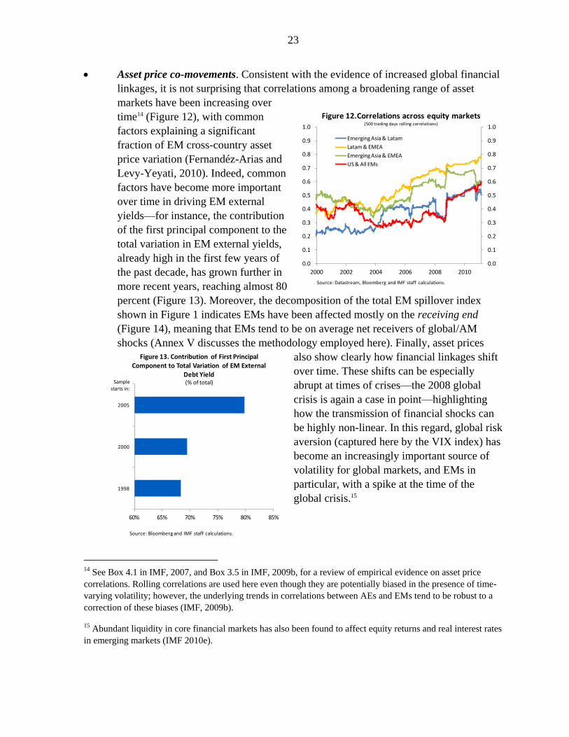
Asset price co-movements. Consistent with the evidence of increased global financial
linkages, it is not surprising that correlations among a broadening range of asset
markets have been increasing over
time14 (Figure 12), with common
factors explaining a significant
fraction of EM cross-country asset
price variation (Fernandéz-Arias and
Levy-Yeyati, 2010). Indeed, common
factors have become more important
over time in driving EM external
yields—for instance, the contribution
of the first principal component to the
total variation in EM external yields,
already high in the first few years of
the past decade, has grown further in
more recent years, reaching almost 80
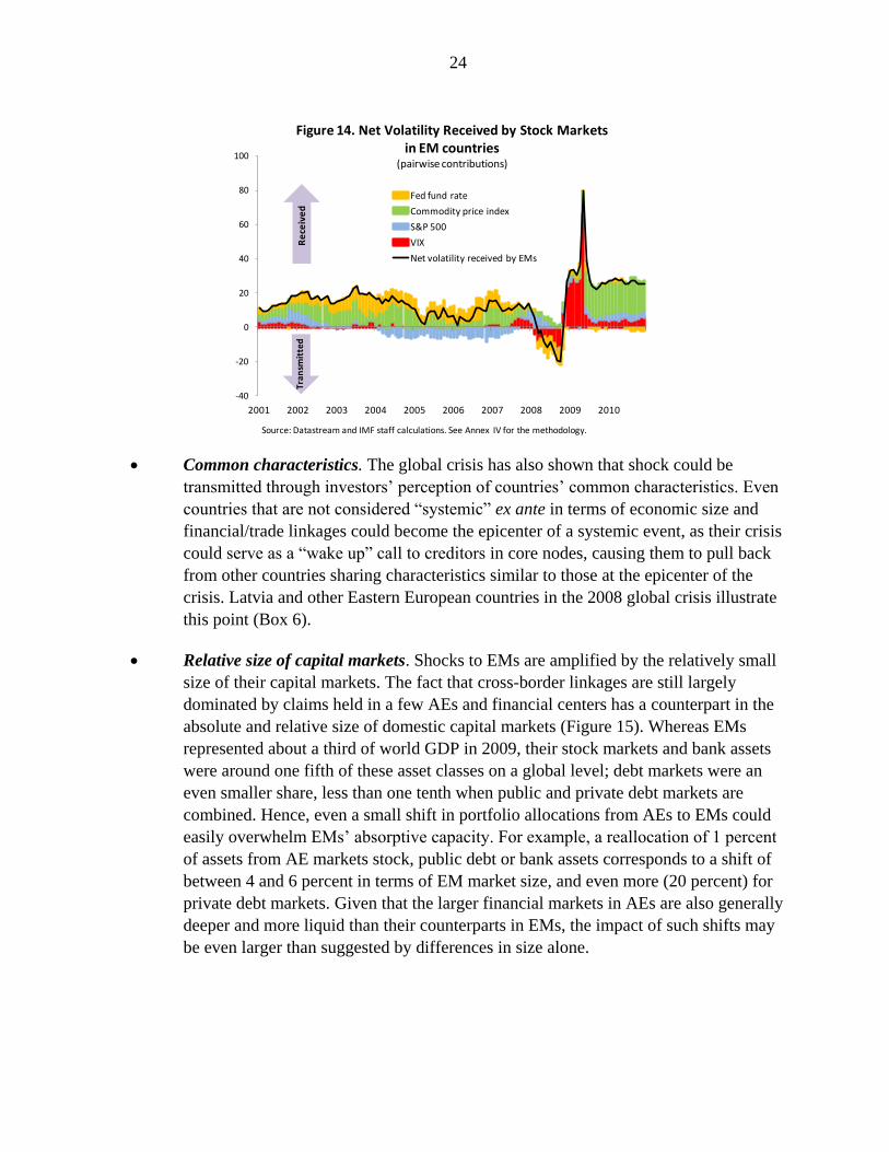
percent (Figure 13). Moreover, the decomposition of the total EM spillover index
shown in Figure 1 indicates EMs have been affected mostly on the receiving end
(Figure 14), meaning that EMs tend to be on average net receivers of global/AM
shocks (Annex V discusses the methodology employed here). Finally, asset prices
also show clearly how financial linkages shift
over time. These shifts can be especially
abrupt at times of crises—the 2008 global
crisis is again a case in point—highlighting
how the transmission of financial shocks can
be highly non-linear. In this regard, global risk
aversion (captured here by the VIX index) has
become an increasingly important source of
volatility for global markets, and EMs in
particular, with a spike at the time of the
global crisis.15
14 See Box 4.1 in IMF, 2007, and Box 3.5 in IMF, 2009b, for a review of empirical evidence on asset price
correlations. Rolling correlations are used here even though they are potentially biased in the presence of time-
varying volatility; however, the underlying trends in correlations between AEs and EMs tend to be robust to a
correction of these biases (IMF, 2009b).
15 Abundant liquidity in core financial markets has also been found to affect equity returns and real interest rates
in emerging markets (IMF 2010e).
24
-40
-20
0
20
40
60
80
100
2001 2002 2003 2004 2005 2006 2007 2008 2009 2010
Fed fund rate
Commodity price index
S&P 500
VIX
Net volatility received by EMs
Figure 14. Net Volatility Received by Stock Marketsin EM countries
(pairwise contributions)
Source: Datastream and IMF staff calculations. See Annex IV for the methodology.
Re
ceiv
ed
Tran
smit
ted
Common characteristics. The global crisis has also shown that shock could be
transmitted through investors‘ perception of countries‘ common characteristics. Even
countries that are not considered ―systemic‖ ex ante in terms of economic size and
financial/trade linkages could become the epicenter of a systemic event, as their crisis
could serve as a ―wake up‖ call to creditors in core nodes, causing them to pull back
from other countries sharing characteristics similar to those at the epicenter of the
crisis. Latvia and other Eastern European countries in the 2008 global crisis illustrate
this point (Box 6).
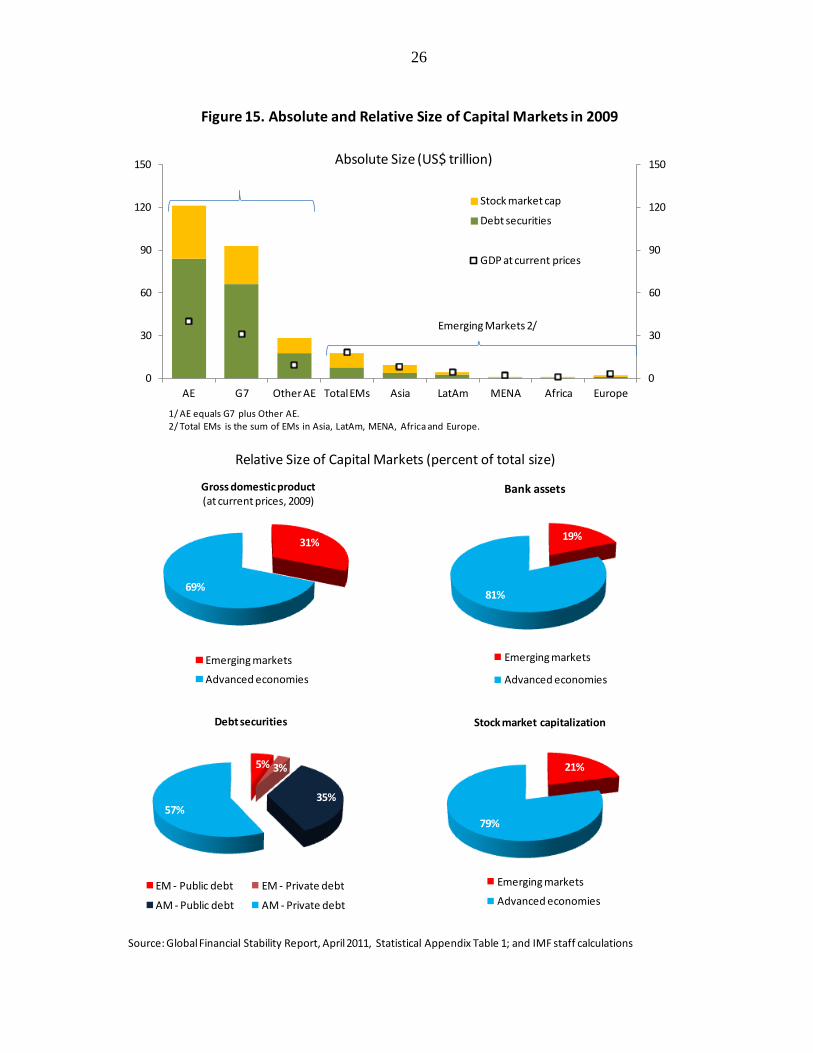
Relative size of capital markets. Shocks to EMs are amplified by the relatively small
size of their capital markets. The fact that cross-border linkages are still largely
dominated by claims held in a few AEs and financial centers has a counterpart in the
absolute and relative size of domestic capital markets (Figure 15). Whereas EMs
represented about a third of world GDP in 2009, their stock markets and bank assets
were around one fifth of these asset classes on a global level; debt markets were an
even smaller share, less than one tenth when public and private debt markets are
combined. Hence, even a small shift in portfolio allocations from AEs to EMs could
easily overwhelm EMs‘ absorptive capacity. For example, a reallocation of 1 percent
of assets from AE markets stock, public debt or bank assets corresponds to a shift of
between 4 and 6 percent in terms of EM market size, and even more (20 percent) for
private debt markets. Given that the larger financial markets in AEs are also generally
deeper and more liquid than their counterparts in EMs, the impact of such shifts may
be even larger than suggested by differences in size alone.
25
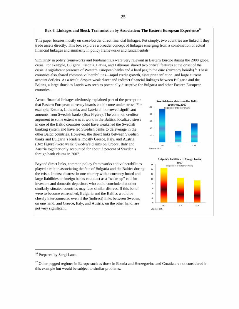
Box 6. Linkages and Shock Transmission by Association: The Eastern European Experience16
This paper focuses mostly on cross-border direct financial linkages. Put simply, two countries are linked if they
trade assets directly. This box explores a broader concept of linkages emerging from a combination of actual
financial linkages and similarity in policy frameworks and fundamentals.
Similarity in policy frameworks and fundamentals were very relevant in Eastern Europe during the 2008 global
crisis. For example, Bulgaria, Estonia, Latvia, and Lithuania shared two critical features at the onset of the
crisis: a significant presence of Western European banks and a hard peg to the euro (currency boards).17 These
countries also shared common vulnerabilities—rapid credit growth, asset price inflation, and large current
account deficits. As a result, despite weak direct and indirect financial linkages between Bulgaria and the
Baltics, a large shock to Latvia was seen as potentially disruptive for Bulgaria and other Eastern European
countries.
Actual financial linkages obviously explained part of the perception
that Eastern European currency boards could come under stress. For
example, Estonia, Lithuania, and Latvia all borrowed significant
amounts from Swedish banks (Box Figure). The common creditor
argument to some extent was at work in the Baltics: localized stress
in one of the Baltic countries could have weakened the Swedish
banking system and have led Swedish banks to deleverage in the
other Baltic countries. However, the direct links between Swedish
banks and Bulgaria‘s lenders, mostly Greece, Italy, and Austria,
(Box Figure) were weak: Sweden‘s claims on Greece, Italy and
Austria together only accounted for about 3 percent of Sweden‘s
foreign bank claims in 2007.
Beyond direct links, common policy frameworks and vulnerabilities
played a role in associating the fate of Bulgaria and the Baltics during
the crisis. Intense distress in one country with a currency board and
large liabilities to foreign banks could act as a ―wake-up‖ call for
investors and domestic depositors who could conclude that other
similarly-situated countries may face similar distress. If this belief
were to become entrenched, Bulgaria and the Baltics would be
closely interconnected even if the (indirect) links between Sweden,
on one hand, and Greece, Italy, and Austria, on the other hand, are
not very significant.
16 Prepared by Sergi Lanau.
17 Other pegged regimes in Europe such as those in Bosnia and Herzegovina and Croatia are not considered in
this example but would be subject to similar problems.
0
2
4
6
8
10
12
14
16
GRC ITA AUT
Bulgaria's liabilities to foreign banks, 2007
(in percent of Bulgaria's GDP)
Source: BIS.
0
20
40
60
80
100
EST LTU LVA
Swedish bank claims on the Baltic countries, 2007
(in percent of debtor's GDP)
Source: BIS.
26
31%
69%
Emerging markets
Advanced economies
Gross domestic product(at current prices, 2009)
21%
79%
Emerging markets
Advanced economies
Stock market capitalization
5% 3%
35%57%
EM - Public debt EM - Private debt
AM - Public debt AM - Private debt
Debt securities
19%
81%
Emerging markets
Advanced economies
Bank assets
0
30
60
90
120
150
0
30
60
90
120
150
AE G7 Other AE Total EMs Asia LatAm MENA Africa Europe
Stock market cap
Debt securities
GDP at current prices
Absolute Size (US$ trillion)
Emerging Markets 2/
1/ AE equals G7 plus Other AE.2/ Total EMs is the sum of EMs in Asia, LatAm, MENA, Africa and Europe.
Relative Size of Capital Markets (percent of total size)
Figure 15. Absolute and Relative Size of Capital Markets in 2009
Source: Global Financial Stability Report, April2011, Statistical Appendix Table 1; and IMF staff calculations
27
-40 -20 0 20 40 60 80
China
Euro, Japan and UK
ROW
Box Figure 1: Estimated Long-Term Impact on Asset Price of China's Current Portfolio
Allocations 1/(in percent)
Sources: World Economic Outlook and staff estimates.1/ Calculations are based on April 2011 WEO.
0 2 4 6 8
U.S.
Euro, Japan and UK
ROW
Box Figure 2. Asset price response to more reserve accumulation from China
(in percent)
More ROW Assets
Current Allocation
Sources: World Economic Outlook and staff estimates.
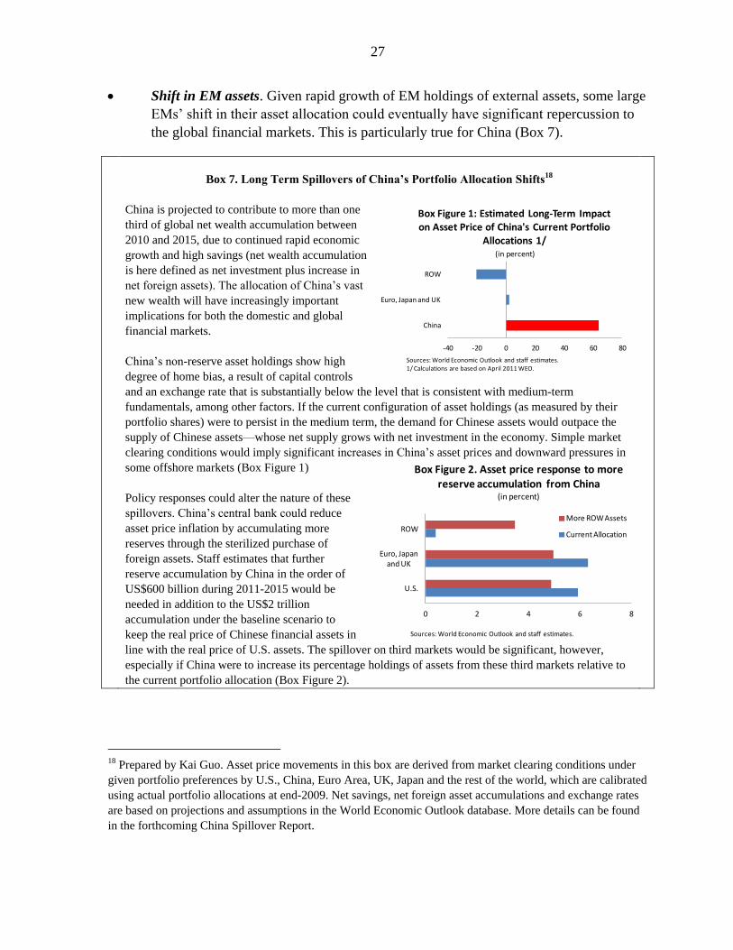
Shift in EM assets. Given rapid growth of EM holdings of external assets, some large
EMs‘ shift in their asset allocation could eventually have significant repercussion to
the global financial markets. This is particularly true for China (Box 7).
Box 7. Long Term Spillovers of China’s Portfolio Allocation Shifts18
China is projected to contribute to more than one
third of global net wealth accumulation between
2010 and 2015, due to continued rapid economic
growth and high savings (net wealth accumulation
is here defined as net investment plus increase in
net foreign assets). The allocation of China‘s vast
new wealth will have increasingly important
implications for both the domestic and global
financial markets.
China‘s non-reserve asset holdings show high
degree of home bias, a result of capital controls
and an exchange rate that is substantially below the level that is consistent with medium-term
fundamentals, among other factors. If the current configuration of asset holdings (as measured by their
portfolio shares) were to persist in the medium term, the demand for Chinese assets would outpace the
supply of Chinese assets—whose net supply grows with net investment in the economy. Simple market
clearing conditions would imply significant increases in China‘s asset prices and downward pressures in
some offshore markets (Box Figure 1)
Policy responses could alter the nature of these
spillovers. China‘s central bank could reduce
asset price inflation by accumulating more
reserves through the sterilized purchase of
foreign assets. Staff estimates that further
reserve accumulation by China in the order of
US$600 billion during 2011-2015 would be
needed in addition to the US$2 trillion
accumulation under the baseline scenario to
keep the real price of Chinese financial assets in
line with the real price of U.S. assets. The spillover on third markets would be significant, however,
especially if China were to increase its percentage holdings of assets from these third markets relative to
the current portfolio allocation (Box Figure 2).
18 Prepared by Kai Guo. Asset price movements in this box are derived from market clearing conditions under
given portfolio preferences by U.S., China, Euro Area, UK, Japan and the rest of the world, which are calibrated
using actual portfolio allocations at end-2009. Net savings, net foreign asset accumulations and exchange rates
are based on projections and assumptions in the World Economic Outlook database. More details can be found
in the forthcoming China Spillover Report.
28
Figure 16. Accumulated Response to GDP Shocks, 1991-2010.
Financial shocksOther shocks
-0.6
0.0
0.6
1.2
1Q 2Q 3Q 4Q 5Q 6Q 7Q 8Q
EMs Response to AMs GDP
-0.6
0.0
0.6
1.2
1Q 2Q 3Q 4Q 5Q 6Q 7Q 8Q
AMs Response to EMs GDP
Source: IMF staff estimation.1/ The AE bloc includes the U.S., the euro area, Japan and the United Kingdom; the EM bloc all the G20 EM countries. Real GDPgrowth was aggregated using PPP weights. The contribution from the financial sector shocks is estimated as the difference in the impulseresponses once short-term and long-term interest rates, and equity prices are included in the VAR regression specification as exogenous variables (following the approach in Bayoumi-Swiston, 2009). The dotted lines indicate two-standard errors confidence bands.
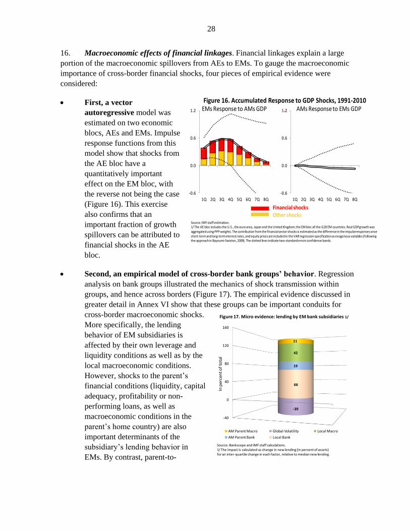
16. Macroeconomic effects of financial linkages. Financial linkages explain a large
portion of the macroeconomic spillovers from AEs to EMs. To gauge the macroeconomic
importance of cross-border financial shocks, four pieces of empirical evidence were
considered:
First, a vector
autoregressive model was
estimated on two economic
blocs, AEs and EMs. Impulse
response functions from this
model show that shocks from
the AE bloc have a
quantitatively important
effect on the EM bloc, with
the reverse not being the case
(Figure 16). This exercise
also confirms that an
important fraction of growth
spillovers can be attributed to
financial shocks in the AE
bloc.
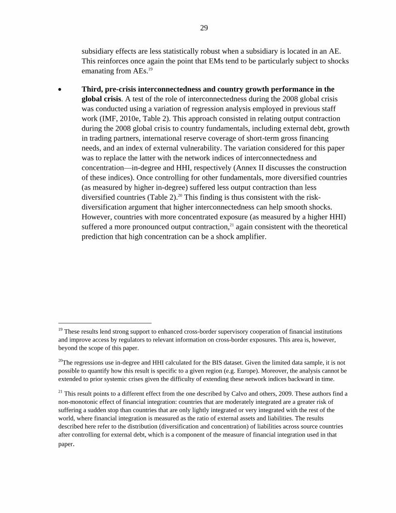
Second, an empirical model of cross-border bank groups’ behavior. Regression
analysis on bank groups illustrated the mechanics of shock transmission within
groups, and hence across borders (Figure 17). The empirical evidence discussed in
greater detail in Annex VI show that these groups can be important conduits for
cross-border macroeconomic shocks.
More specifically, the lending
behavior of EM subsidiaries is
affected by their own leverage and
liquidity conditions as well as by the
local macroeconomic conditions.
However, shocks to the parent‘s
financial conditions (liquidity, capital
adequacy, profitability or non-
performing loans, as well as
macroeconomic conditions in the
parent‘s home country) are also
important determinants of the
subsidiary‘s lending behavior in
EMs. By contrast, parent-to-
-40
0
40
80
120
160
66
19
42
-39
11
In p
erce
nt o
f to
tal
AM Parent Macro Global Volatility Local Macro
AM Parent Bank Local Bank
Figure 17. Micro evidence: lending by EM bank subsidiaries 1/
Source: Bankscope and IMF staff calculations.1/ The impact is calculated as change in new lending (in percent of assets)for an inter-quartile change in each factor, relative to median new lending.
29
subsidiary effects are less statistically robust when a subsidiary is located in an AE.
This reinforces once again the point that EMs tend to be particularly subject to shocks
emanating from AEs.19
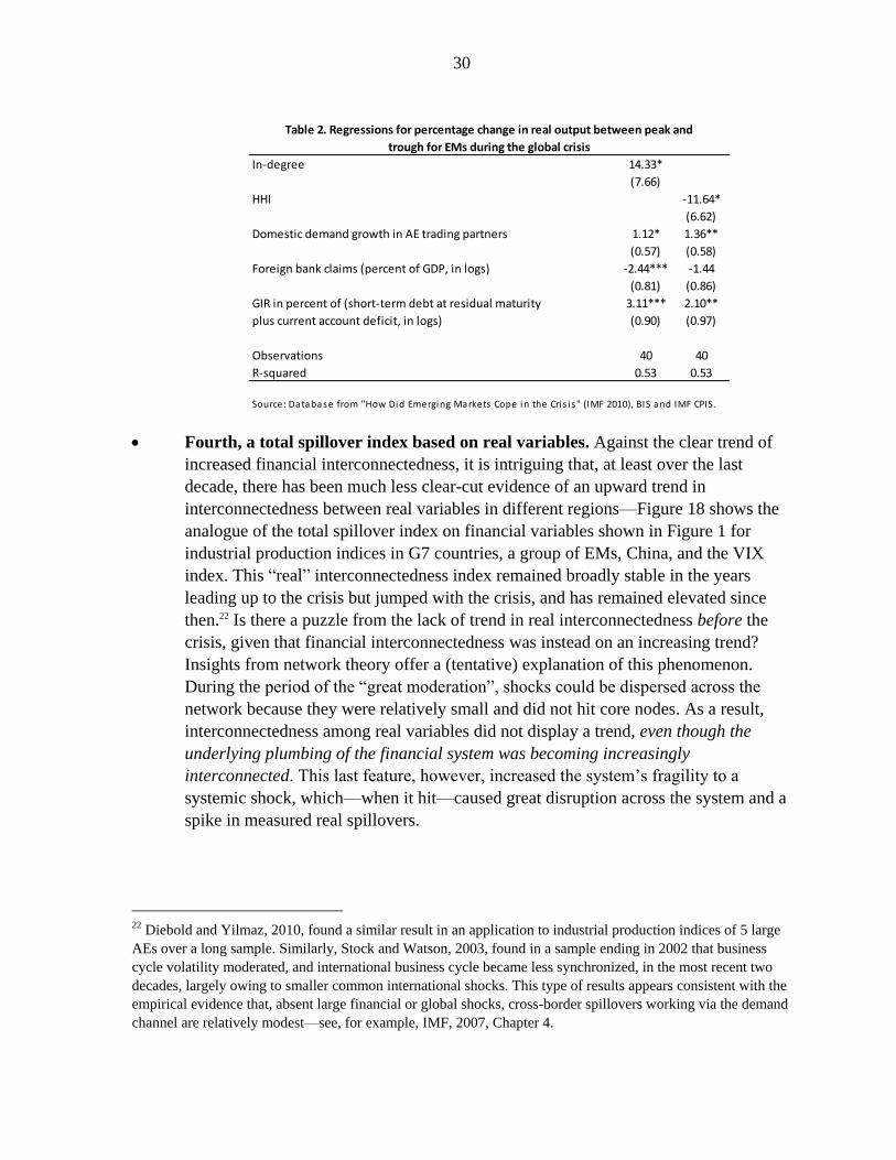
Third, pre-crisis interconnectedness and country growth performance in the
global crisis. A test of the role of interconnectedness during the 2008 global crisis
was conducted using a variation of regression analysis employed in previous staff
work (IMF, 2010e, Table 2). This approach consisted in relating output contraction
during the 2008 global crisis to country fundamentals, including external debt, growth
in trading partners, international reserve coverage of short-term gross financing
needs, and an index of external vulnerability. The variation considered for this paper
was to replace the latter with the network indices of interconnectedness and
concentration—in-degree and HHI, respectively (Annex II discusses the construction
of these indices). Once controlling for other fundamentals, more diversified countries
(as measured by higher in-degree) suffered less output contraction than less
diversified countries (Table 2).20 This finding is thus consistent with the risk-
diversification argument that higher interconnectedness can help smooth shocks.
However, countries with more concentrated exposure (as measured by a higher HHI)
suffered a more pronounced output contraction,21 again consistent with the theoretical
prediction that high concentration can be a shock amplifier.
19 These results lend strong support to enhanced cross-border supervisory cooperation of financial institutions
and improve access by regulators to relevant information on cross-border exposures. This area is, however,
beyond the scope of this paper.
20The regressions use in-degree and HHI calculated for the BIS dataset. Given the limited data sample, it is not
possible to quantify how this result is specific to a given region (e.g. Europe). Moreover, the analysis cannot be
extended to prior systemic crises given the difficulty of extending these network indices backward in time.
21 This result points to a different effect from the one described by Calvo and others, 2009. These authors find a
non-monotonic effect of financial integration: countries that are moderately integrated are a greater risk of
suffering a sudden stop than countries that are only lightly integrated or very integrated with the rest of the
world, where financial integration is measured as the ratio of external assets and liabilities. The results
described here refer to the distribution (diversification and concentration) of liabilities across source countries
after controlling for external debt, which is a component of the measure of financial integration used in that
paper.
30
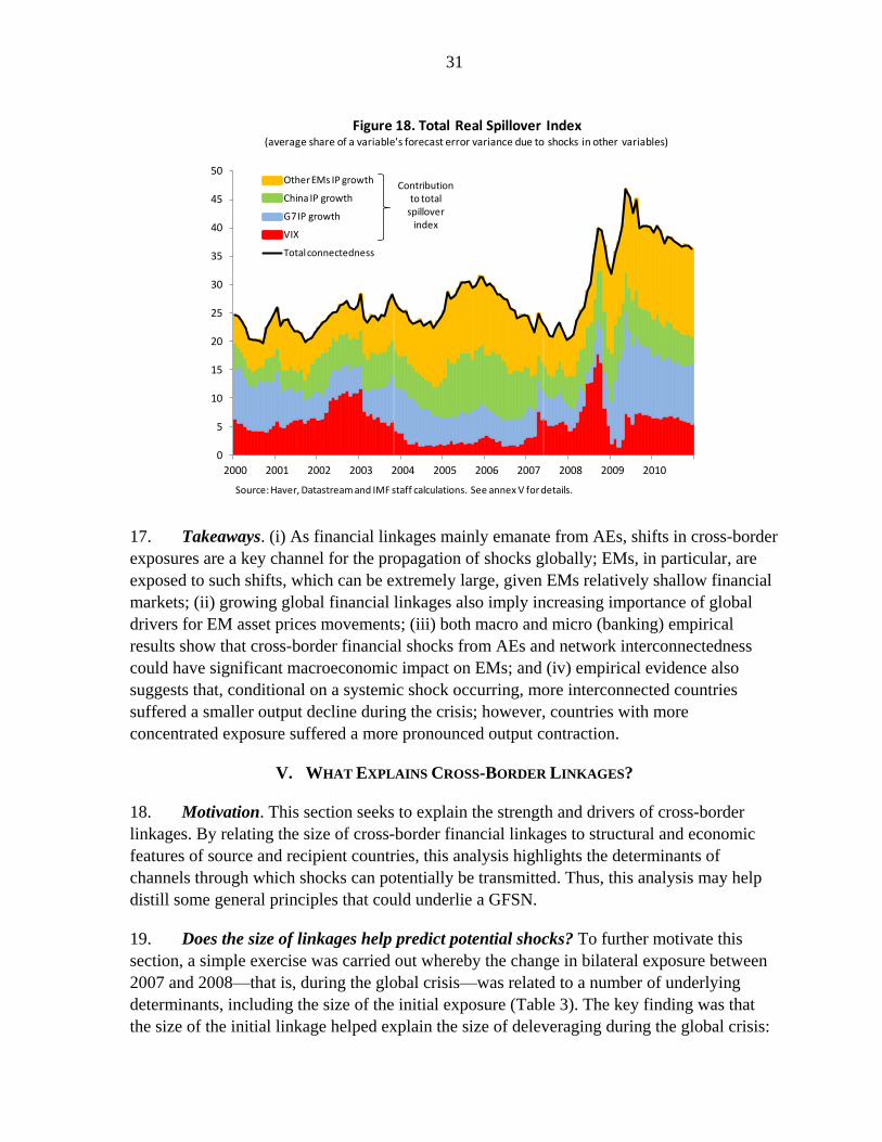
Fourth, a total spillover index based on real variables. Against the clear trend of
increased financial interconnectedness, it is intriguing that, at least over the last
decade, there has been much less clear-cut evidence of an upward trend in
interconnectedness between real variables in different regions—Figure 18 shows the
analogue of the total spillover index on financial variables shown in Figure 1 for
industrial production indices in G7 countries, a group of EMs, China, and the VIX
index. This ―real‖ interconnectedness index remained broadly stable in the years
leading up to the crisis but jumped with the crisis, and has remained elevated since
then.22 Is there a puzzle from the lack of trend in real interconnectedness before the
crisis, given that financial interconnectedness was instead on an increasing trend?
Insights from network theory offer a (tentative) explanation of this phenomenon.
During the period of the ―great moderation‖, shocks could be dispersed across the
network because they were relatively small and did not hit core nodes. As a result,
interconnectedness among real variables did not display a trend, even though the
underlying plumbing of the financial system was becoming increasingly
interconnected. This last feature, however, increased the system‘s fragility to a
systemic shock, which—when it hit—caused great disruption across the system and a
spike in measured real spillovers.
22 Diebold and Yilmaz, 2010, found a similar result in an application to industrial production indices of 5 large
AEs over a long sample. Similarly, Stock and Watson, 2003, found in a sample ending in 2002 that business
cycle volatility moderated, and international business cycle became less synchronized, in the most recent two
decades, largely owing to smaller common international shocks. This type of results appears consistent with the
empirical evidence that, absent large financial or global shocks, cross-border spillovers working via the demand
channel are relatively modest—see, for example, IMF, 2007, Chapter 4.
In-degree 14.33*
(7.66)
HHI -11.64*
(6.62)
Domestic demand growth in AE trading partners 1.12* 1.36**
(0.57) (0.58)
Foreign bank claims (percent of GDP, in logs) -2.44*** -1.44
(0.81) (0.86)
GIR in percent of (short-term debt at residual maturity 3.11*** 2.10**
plus current account deficit, in logs) (0.90) (0.97)
Observations 40 40
R-squared 0.53 0.53
Source: Database from "How Did Emerging Markets Cope in the Cris is" (IMF 2010), BIS and IMF CPIS.
Table 2. Regressions for percentage change in real output between peak and
trough for EMs during the global crisis
31
17. Takeaways. (i) As financial linkages mainly emanate from AEs, shifts in cross-border
exposures are a key channel for the propagation of shocks globally; EMs, in particular, are
exposed to such shifts, which can be extremely large, given EMs relatively shallow financial
markets; (ii) growing global financial linkages also imply increasing importance of global
drivers for EM asset prices movements; (iii) both macro and micro (banking) empirical
results show that cross-border financial shocks from AEs and network interconnectedness
could have significant macroeconomic impact on EMs; and (iv) empirical evidence also
suggests that, conditional on a systemic shock occurring, more interconnected countries
suffered a smaller output decline during the crisis; however, countries with more
concentrated exposure suffered a more pronounced output contraction.
V. WHAT EXPLAINS CROSS-BORDER LINKAGES?
18. Motivation. This section seeks to explain the strength and drivers of cross-border
linkages. By relating the size of cross-border financial linkages to structural and economic
features of source and recipient countries, this analysis highlights the determinants of
channels through which shocks can potentially be transmitted. Thus, this analysis may help
distill some general principles that could underlie a GFSN.
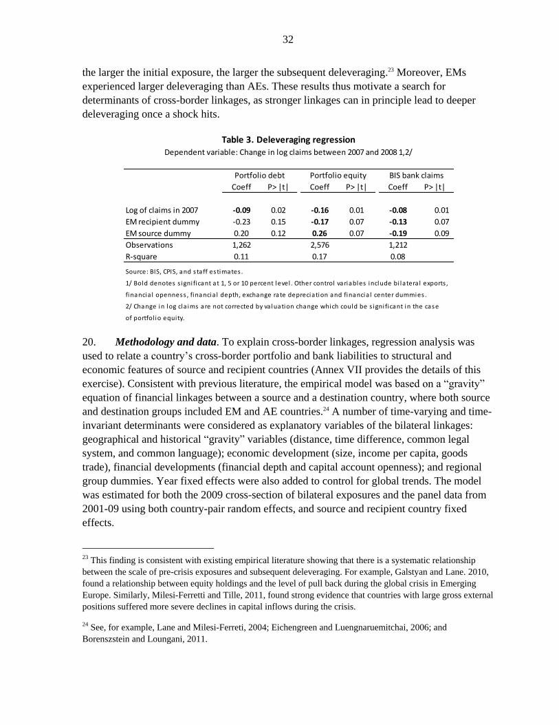
19. Does the size of linkages help predict potential shocks? To further motivate this
section, a simple exercise was carried out whereby the change in bilateral exposure between
2007 and 2008—that is, during the global crisis—was related to a number of underlying
determinants, including the size of the initial exposure (Table 3). The key finding was that
the size of the initial linkage helped explain the size of deleveraging during the global crisis:
0
5
10
15
20
25
30
35
40
45
50
2000 2001 2002 2003 2004 2005 2006 2007 2008 2009 2010
Other EMs IP growth
China IP growth
G7 IP growth
VIX
Total connectedness
Contribution to total
spillover index
Source: Haver, Datastream and IMF staff calculations. See annex V for details.
Figure 18. Total Real Spillover Index(average share of a variable's forecast error variance due to shocks in other variables)
32
the larger the initial exposure, the larger the subsequent deleveraging.23 Moreover, EMs
experienced larger deleveraging than AEs. These results thus motivate a search for
determinants of cross-border linkages, as stronger linkages can in principle lead to deeper
deleveraging once a shock hits.
20. Methodology and data. To explain cross-border linkages, regression analysis was
used to relate a country‘s cross-border portfolio and bank liabilities to structural and
economic features of source and recipient countries (Annex VII provides the details of this
exercise). Consistent with previous literature, the empirical model was based on a ―gravity‖
equation of financial linkages between a source and a destination country, where both source
and destination groups included EM and AE countries.24 A number of time-varying and time-
invariant determinants were considered as explanatory variables of the bilateral linkages:
geographical and historical ―gravity‖ variables (distance, time difference, common legal
system, and common language); economic development (size, income per capita, goods
trade), financial developments (financial depth and capital account openness); and regional
group dummies. Year fixed effects were also added to control for global trends. The model
was estimated for both the 2009 cross-section of bilateral exposures and the panel data from
2001-09 using both country-pair random effects, and source and recipient country fixed
effects.
23 This finding is consistent with existing empirical literature showing that there is a systematic relationship
between the scale of pre-crisis exposures and subsequent deleveraging. For example, Galstyan and Lane. 2010,
found a relationship between equity holdings and the level of pull back during the global crisis in Emerging
Europe. Similarly, Milesi-Ferretti and Tille, 2011, found strong evidence that countries with large gross external
positions suffered more severe declines in capital inflows during the crisis.
24 See, for example, Lane and Milesi-Ferreti, 2004; Eichengreen and Luengnaruemitchai, 2006; and
Borenszstein and Loungani, 2011.
Coeff P> |t| Coeff P> |t| Coeff P> |t|
Log of claims in 2007 -0.09 0.02 -0.16 0.01 -0.08 0.01
EM recipient dummy -0.23 0.15 -0.17 0.07 -0.13 0.07
EM source dummy 0.20 0.12 0.26 0.07 -0.19 0.09
Observations 1,262 2,576 1,212
R-square 0.11 0.17 0.08
Source: BIS, CPIS, and s taff estimates .
1/ Bold denotes s igni ficant at 1, 5 or 10 percent level . Other control variables include bi latera l exports ,
financia l openness , financia l depth, exchange rate depreciation and financia l center dummies .
2/ Change in log cla ims are not corrected by va luation change which could be s igni ficant in the case
of portfol io equity.
Table 3. Deleveraging regressionDependent variable: Change in log claims between 2007 and 2008 1,2/
Portfolio debt Portfolio equity BIS bank claims
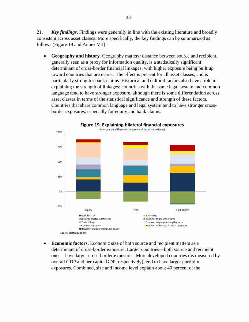
33
21. Key findings. Findings were generally in line with the existing literature and broadly
consistent across asset classes. More specifically, the key findings can be summarized as
follows (Figure 19 and Annex VII):
Geography and history. Geography matters: distance between source and recipient,
generally seen as a proxy for information quality, is a statistically significant
determinant of cross-border financial linkages, with higher exposure being built up
toward countries that are nearer. The effect is present for all asset classes, and is
particularly strong for bank claims. Historical and cultural factors also have a role in
explaining the strength of linkages: countries with the same legal system and common
language tend to have stronger exposure, although there is some differentiation across
asset classes in terms of the statistical significance and strength of these factors.
Countries that share common language and legal system tend to have stronger cross-
border exposures, especially for equity and bank claims.
Economic factors. Economic size of both source and recipient matters as a
determinant of cross-border exposure. Larger countries—both source and recipient
ones—have larger cross-border exposures. More developed countries (as measured by
overall GDP and per capita GDP, respectively) tend to have larger portfolio
exposures. Combined, size and income level explain about 40 percent of the
-25%
0%
25%
50%
75%
100%
Equity Debt Bank claims
Figure 19. Explaining bilateral financial exposures(Interquartile differences, in percent of the explained part)
Recipient size Source size
Distance and time difference Recipient and source income
Trade linkage Common language and legal system
Common currency Recipient and source financial openness
Recipient and source financial depth
Source: Staff calculations
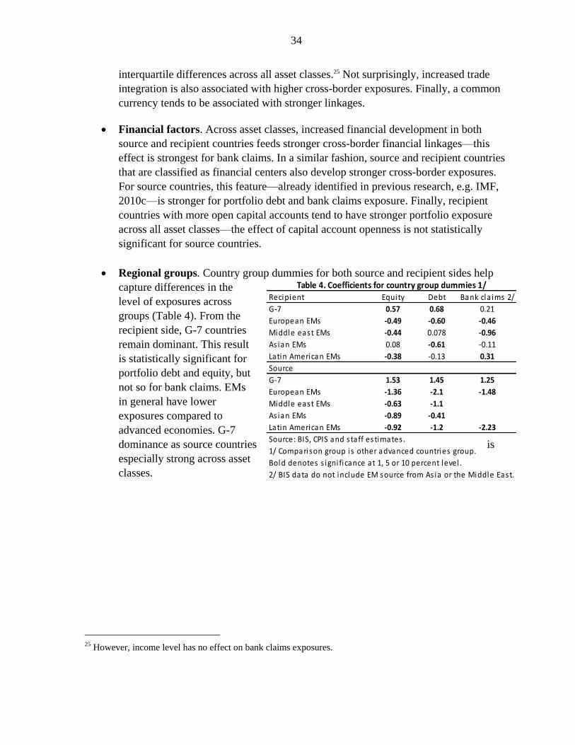
34
Recipient Equity Debt Bank cla ims 2/
G-7 0.57 0.68 0.21
European EMs -0.49 -0.60 -0.46
Middle east EMs -0.44 0.078 -0.96
Asian EMs 0.08 -0.61 -0.11
Latin American EMs -0.38 -0.13 0.31
Source
G-7 1.53 1.45 1.25
European EMs -1.36 -2.1 -1.48
Middle east EMs -0.63 -1.1
Asian EMs -0.89 -0.41
Latin American EMs -0.92 -1.2 -2.23
Source: BIS, CPIS and s taff estimates .
1/ Comparison group is other advanced countries group.
Bold denotes s igni ficance at 1, 5 or 10 percent level .
2/ BIS data do not include EM source from As ia or the Middle East.
Table 4. Coefficients for country group dummies 1/
interquartile differences across all asset classes.25 Not surprisingly, increased trade
integration is also associated with higher cross-border exposures. Finally, a common
currency tends to be associated with stronger linkages.
Financial factors. Across asset classes, increased financial development in both
source and recipient countries feeds stronger cross-border financial linkages—this
effect is strongest for bank claims. In a similar fashion, source and recipient countries
that are classified as financial centers also develop stronger cross-border exposures.
For source countries, this feature—already identified in previous research, e.g. IMF,
2010c—is stronger for portfolio debt and bank claims exposure. Finally, recipient
countries with more open capital accounts tend to have stronger portfolio exposure
across all asset classes—the effect of capital account openness is not statistically
significant for source countries.
Regional groups. Country group dummies for both source and recipient sides help
capture differences in the
level of exposures across
groups (Table 4). From the
recipient side, G-7 countries
remain dominant. This result
is statistically significant for
portfolio debt and equity, but
not so for bank claims. EMs
in general have lower
exposures compared to
advanced economies. G-7
dominance as source countries is
especially strong across asset
classes.
25 However, income level has no effect on bank claims exposures.
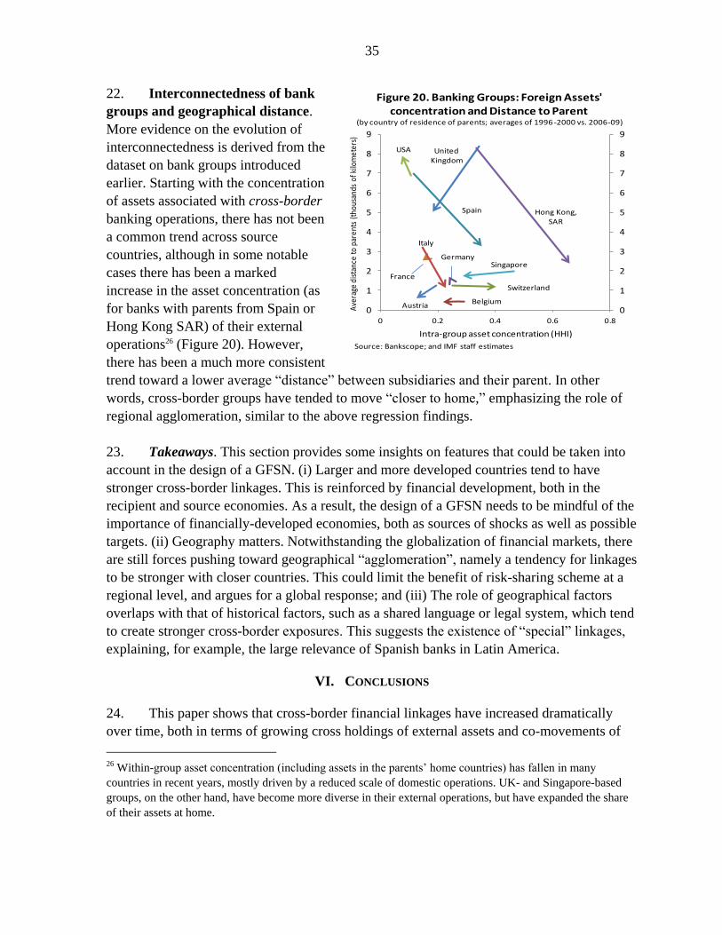
35
AustriaBelgium
Switzerland
Germany
Spain
France
United Kingdom
Italy
USA
Hong Kong, SAR
Singapore
0
1
2
3
4
5
6
7
8
9
0
1
2
3
4
5
6
7
8
9
0 0.2 0.4 0.6 0.8
Ave
rage
dist
ance
to p
aren
ts (
thou
sand
s of
kilo
met
ers)
Figure 20. Banking Groups: Foreign Assets' concentration and Distance to Parent
(by country of residence of parents; averages of 1996 -2000 vs. 2006-09)
Source: Bankscope; and IMF staff estimates
Intra-group asset concentration (HHI)
22. Interconnectedness of bank
groups and geographical distance.
More evidence on the evolution of
interconnectedness is derived from the
dataset on bank groups introduced
earlier. Starting with the concentration
of assets associated with cross-border
banking operations, there has not been
a common trend across source
countries, although in some notable
cases there has been a marked
increase in the asset concentration (as
for banks with parents from Spain or
Hong Kong SAR) of their external
operations26 (Figure 20). However,
there has been a much more consistent
trend toward a lower average ―distance‖ between subsidiaries and their parent. In other
words, cross-border groups have tended to move ―closer to home,‖ emphasizing the role of
regional agglomeration, similar to the above regression findings.
23. Takeaways. This section provides some insights on features that could be taken into
account in the design of a GFSN. (i) Larger and more developed countries tend to have
stronger cross-border linkages. This is reinforced by financial development, both in the
recipient and source economies. As a result, the design of a GFSN needs to be mindful of the
importance of financially-developed economies, both as sources of shocks as well as possible
targets. (ii) Geography matters. Notwithstanding the globalization of financial markets, there
are still forces pushing toward geographical ―agglomeration‖, namely a tendency for linkages
to be stronger with closer countries. This could limit the benefit of risk-sharing scheme at a
regional level, and argues for a global response; and (iii) The role of geographical factors
overlaps with that of historical factors, such as a shared language or legal system, which tend
to create stronger cross-border exposures. This suggests the existence of ―special‖ linkages,
explaining, for example, the large relevance of Spanish banks in Latin America.
VI. CONCLUSIONS
24. This paper shows that cross-border financial linkages have increased dramatically
over time, both in terms of growing cross holdings of external assets and co-movements of
26 Within-group asset concentration (including assets in the parents‘ home countries) has fallen in many
countries in recent years, mostly driven by a reduced scale of domestic operations. UK- and Singapore-based
groups, on the other hand, have become more diverse in their external operations, but have expanded the share
of their assets at home.
36
asset prices across asset classes and economies. These linkages are still dominated by a few
AEs and financial centers, which form ―core nodes‖ in the system. EMs‘ cross-border
holdings, despite having experienced rapid growth in the last decade, remain relatively small,
while the bulk of EMs‘ liabilities are held by core nodes. EMs, with shallow domestic capital
markets, are particularly exposed to large shifts in cross-border exposures. The empirical
evidence in this paper suggests that shocks can be highly synchronized across global
financial markets and their transmission non-linear, potentially carrying significant real costs
to EM economies.
25. Efforts to increase the resilience of the global financial system face a delicate trade-
off between the benefits at the country level from increased international risk
diversification—a force that pushes toward increasing the system‘s overall
interconnectedness—and the increased systemic risk that this heightened interconnectedness
generates at the global level. National defenses, including via self-insurance, may not be able
to eliminate the externalities intrinsic in an interconnected financial network. To the extent
that national defenses are insufficient to reduce the source of volatility and instability
inherent with the global financial system, regional and, especially, global financing
mechanisms have a role to play in cushioning the impact of residual volatility on countries
and the system at large. The recent global crisis underscores the value of an effective global
mechanism to coordinate liquidity injections and other policy responses: in 2008-09, a
number of countries with relatively strong fundamentals (―crisis bystanders‖) were hit later
and less severely than countries with weaker fundamentals, and were able to recover from the
crisis more rapidly; but they still suffered a deep output contraction. This, combined with the
limited opportunities to diversify against the risk of cross-border shocks, points to the
significant gains from a global financial safety net that is effective in forestalling localized
liquidity runs to turn into systemic crises.
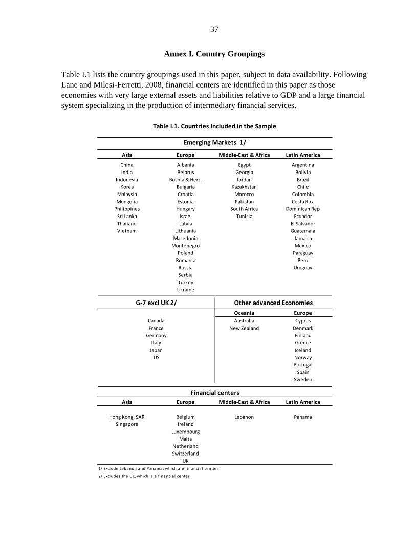
37
Annex I. Country Groupings
Table I.1 lists the country groupings used in this paper, subject to data availability. Following
Lane and Milesi-Ferretti, 2008, financial centers are identified in this paper as those
economies with very large external assets and liabilities relative to GDP and a large financial
system specializing in the production of intermediary financial services.
Asia Europe Middle-East & Africa Latin America
China Albania Egypt Argentina
India Belarus Georgia Bolivia
Indonesia Bosnia & Herz. Jordan Brazil
Korea Bulgaria Kazakhstan Chile
Malaysia Croatia Morocco Colombia
Mongolia Estonia Pakistan Costa Rica
Philippines Hungary South Africa Dominican Rep
Sri Lanka Israel Tunisia Ecuador
Thailand Latvia El Salvador
Vietnam Lithuania Guatemala
Macedonia Jamaica
Montenegro Mexico
Poland Paraguay
Romania Peru
Russia Uruguay
Serbia
Turkey
Ukraine
Oceania Europe
Australia Cyprus
New Zealand Denmark
Finland
Greece
Iceland
Norway
Portugal
Spain
Sweden
Asia Europe Middle-East & Africa Latin America
Hong Kong, SAR Belgium Lebanon Panama
Singapore Ireland
Luxembourg
Malta
Netherland
Switzerland
UK
1/ Exclude Lebanon and Panama, which are financia l centers .
2/ Excludes the UK, which i s a financia l center.
Emerging Markets 1/
Financial centers
Table I.1. Countries Included in the Sample
Other advanced EconomiesG-7 excl UK 2/
Canada
France
Germany
Italy
Japan
US
38
Annex II. Network Analysis27
This annex first provides a short review of network theory and then describes the
methodology and data used in measuring a country‘s financial interconnectedness with the
rest of the world and the concentration of its cross-border exposures.
Insights from network theory
Network analysis. Many of the financial market phenomena described in this paper can be
seen—using insights from network theory—as the result of increased interconnectedness in a
financial network. Besides the staff work mentioned in the paper, a growing literature has
examined the properties of financial networks and their implications for financial stability
(see Haldane, 2009, for an excellent overview of the field; there have also been a number of
application of network analysis to financial stability issues by staff, see, e.g., IMF, 2009a). In
particular, the seminal contribution by Allen and Gale, 2005, showed that—in the absence of
financial frictions—more interconnectedness increases risk diversification and makes the
network more robust. Subsequent research has shown, however, that in the presence of
financial frictions, high levels of interconnectedness may increase systemic risk (Battistion
and others, 2009, and Gai and Kapadia, 2008). Finally, a number of papers have used a range
of network statistics to describe the financial network and patterns of stress transmission
(Garrat and others, 2011, Kubelec and Sa, 2010, von Peter, 2007).
Interconnectedness as a double-edged sword. The key insight of network theory applied to
financial stability analysis is that interconnectedness is a double-edged sword.
Interconnectedness has the potential of making a network more robust, but it also increases
the risk of rare but devastating events. At low levels, an increase in interconnectedness
improves the resilience of a network; at high levels, however, it may raise the network‘s
latent fragility and vulnerability to systemic breakdowns. The latent fragility of complex
networks is a key rationale for the existence and appropriate design of a GFSN.
“Robust” networks. Recipient countries with a larger number of cross-border links tend to
benefit from better risk diversification of sources,28 as a localized shock hitting a single
source country and the ensuing deleveraging can be more manageable. The opposite is true in
a network with few links.29 This diversification argument—formalized by Allen and Gale,
27 Prepared by Ran Bi and Sergi Lanau.
28 In this context, a link is represented by the stock of claims issued by a recipient country to a source country.
The resulting network corresponds to the visual representation of Figure 2.
29 This narrative assumes that shocks are transmitted through countries as sources reduce their claims on other
countries. This is consistent with the view that rapid deleveraging following a shock to a source is the key
transmission channel of cross-border shocks, especially at times of systemic distress. However, it abstracts from
the specific source of shocks triggering this deleveraging.
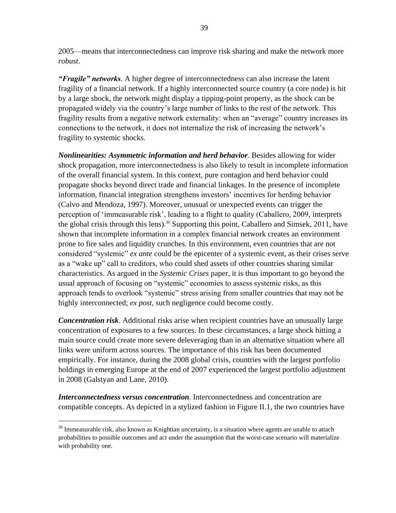
39
2005—means that interconnectedness can improve risk sharing and make the network more
robust.
“Fragile” networks. A higher degree of interconnectedness can also increase the latent
fragility of a financial network. If a highly interconnected source country (a core node) is hit
by a large shock, the network might display a tipping-point property, as the shock can be
propagated widely via the country‘s large number of links to the rest of the network. This
fragility results from a negative network externality: when an ―average‖ country increases its
connections to the network, it does not internalize the risk of increasing the network‘s
fragility to systemic shocks.
Nonlinearities: Asymmetric information and herd behavior. Besides allowing for wider
shock propagation, more interconnectedness is also likely to result in incomplete information
of the overall financial system. In this context, pure contagion and herd behavior could
propagate shocks beyond direct trade and financial linkages. In the presence of incomplete
information, financial integration strengthens investors‘ incentives for herding behavior
(Calvo and Mendoza, 1997). Moreover, unusual or unexpected events can trigger the
perception of ‗immeasurable risk‘, leading to a flight to quality (Caballero, 2009, interprets
the global crisis through this lens).30 Supporting this point, Caballero and Simsek, 2011, have
shown that incomplete information in a complex financial network creates an environment
prone to fire sales and liquidity crunches. In this environment, even countries that are not
considered ―systemic‖ ex ante could be the epicenter of a systemic event, as their crises serve
as a ―wake up‖ call to creditors, who could shed assets of other countries sharing similar
characteristics. As argued in the Systemic Crises paper, it is thus important to go beyond the
usual approach of focusing on ―systemic‖ economies to assess systemic risks, as this
approach tends to overlook ―systemic‖ stress arising from smaller countries that may not be
highly interconnected; ex post, such negligence could become costly.
Concentration risk. Additional risks arise when recipient countries have an unusually large
concentration of exposures to a few sources. In these circumstances, a large shock hitting a
main source could create more severe deleveraging than in an alternative situation where all
links were uniform across sources. The importance of this risk has been documented
empirically. For instance, during the 2008 global crisis, countries with the largest portfolio
holdings in emerging Europe at the end of 2007 experienced the largest portfolio adjustment
in 2008 (Galstyan and Lane, 2010).
Interconnectedness versus concentration. Interconnectedness and concentration are
compatible concepts. As depicted in a stylized fashion in Figure II.1, the two countries have
30 Immeasurable risk, also known as Knightian uncertainty, is a situation where agents are unable to attach
probabilities to possible outcomes and act under the assumption that the worst-case scenario will materialize
with probability one.
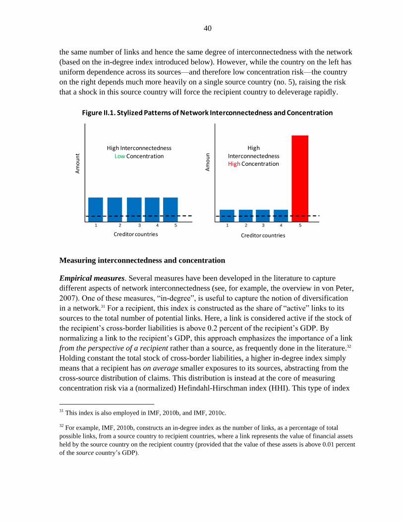
40
the same number of links and hence the same degree of interconnectedness with the network
(based on the in-degree index introduced below). However, while the country on the left has
uniform dependence across its sources—and therefore low concentration risk—the country
on the right depends much more heavily on a single source country (no. 5), raising the risk
that a shock in this source country will force the recipient country to deleverage rapidly.
Measuring interconnectedness and concentration
Empirical measures. Several measures have been developed in the literature to capture
different aspects of network interconnectedness (see, for example, the overview in von Peter,
2007). One of these measures, ―in-degree‖, is useful to capture the notion of diversification
in a network.31 For a recipient, this index is constructed as the share of ―active‖ links to its
sources to the total number of potential links. Here, a link is considered active if the stock of
the recipient‘s cross-border liabilities is above 0.2 percent of the recipient‘s GDP. By
normalizing a link to the recipient‘s GDP, this approach emphasizes the importance of a link
from the perspective of a recipient rather than a source, as frequently done in the literature.32
Holding constant the total stock of cross-border liabilities, a higher in-degree index simply
means that a recipient has on average smaller exposures to its sources, abstracting from the
cross-source distribution of claims. This distribution is instead at the core of measuring
concentration risk via a (normalized) Hefindahl-Hirschman index (HHI). This type of index
31 This index is also employed in IMF, 2010b, and IMF, 2010c.
32 For example, IMF, 2010b, constructs an in-degree index as the number of links, as a percentage of total
possible links, from a source country to recipient countries, where a link represents the value of financial assets
held by the source country on the recipient country (provided that the value of these assets is above 0.01 percent
of the source country‘s GDP).
1 2 3 4 5 1 2 3 4 5
Creditor countries Creditor countries
High Interconnectedness
Low Concentration
High
InterconnectednessHigh Concentration
Am
ou
nt
Am
ou
n
Figure II.1. Stylized Patterns of Network Interconnectedness and Concentration
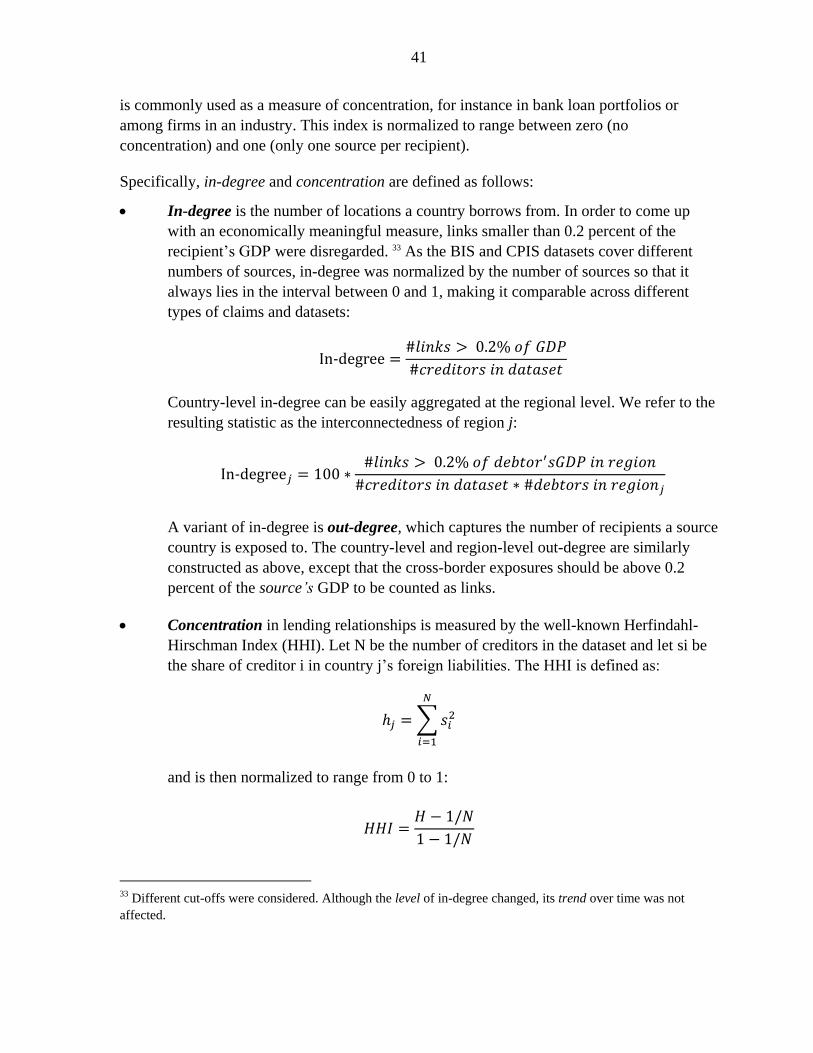
41
is commonly used as a measure of concentration, for instance in bank loan portfolios or
among firms in an industry. This index is normalized to range between zero (no
concentration) and one (only one source per recipient).
Specifically, in-degree and concentration are defined as follows:
In-degree is the number of locations a country borrows from. In order to come up
with an economically meaningful measure, links smaller than 0.2 percent of the
recipient‘s GDP were disregarded. 33 As the BIS and CPIS datasets cover different
numbers of sources, in-degree was normalized by the number of sources so that it
always lies in the interval between 0 and 1, making it comparable across different
types of claims and datasets:
Country-level in-degree can be easily aggregated at the regional level. We refer to the
resulting statistic as the interconnectedness of region j:
A variant of in-degree is out-degree, which captures the number of recipients a source
country is exposed to. The country-level and region-level out-degree are similarly
constructed as above, except that the cross-border exposures should be above 0.2
percent of the source’s GDP to be counted as links.
Concentration in lending relationships is measured by the well-known Herfindahl-
Hirschman Index (HHI). Let N be the number of creditors in the dataset and let si be
the share of creditor i in country j‘s foreign liabilities. The HHI is defined as:
and is then normalized to range from 0 to 1:
33 Different cut-offs were considered. Although the level of in-degree changed, its trend over time was not
affected.
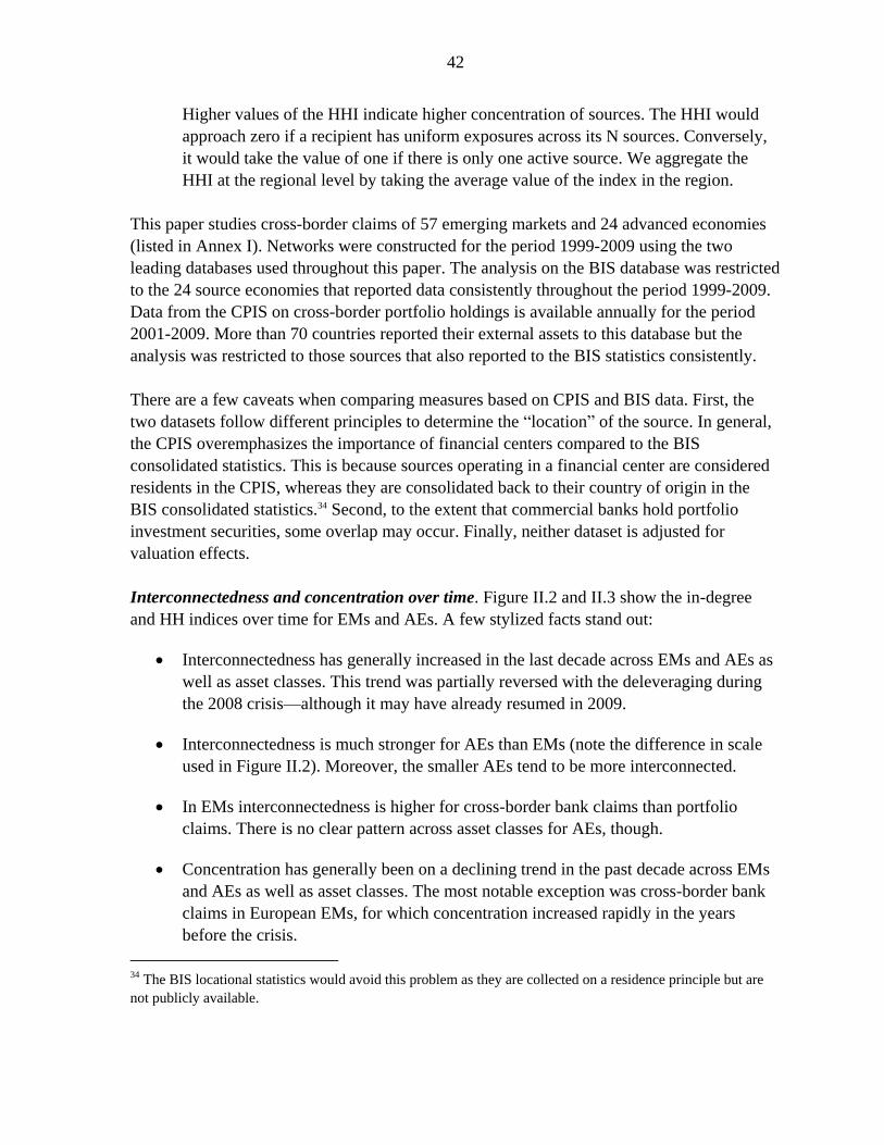
42
Higher values of the HHI indicate higher concentration of sources. The HHI would
approach zero if a recipient has uniform exposures across its N sources. Conversely,
it would take the value of one if there is only one active source. We aggregate the
HHI at the regional level by taking the average value of the index in the region.
This paper studies cross-border claims of 57 emerging markets and 24 advanced economies
(listed in Annex I). Networks were constructed for the period 1999-2009 using the two
leading databases used throughout this paper. The analysis on the BIS database was restricted
to the 24 source economies that reported data consistently throughout the period 1999-2009.
Data from the CPIS on cross-border portfolio holdings is available annually for the period
2001-2009. More than 70 countries reported their external assets to this database but the
analysis was restricted to those sources that also reported to the BIS statistics consistently.
There are a few caveats when comparing measures based on CPIS and BIS data. First, the
two datasets follow different principles to determine the ―location‖ of the source. In general,
the CPIS overemphasizes the importance of financial centers compared to the BIS
consolidated statistics. This is because sources operating in a financial center are considered
residents in the CPIS, whereas they are consolidated back to their country of origin in the
BIS consolidated statistics.34 Second, to the extent that commercial banks hold portfolio
investment securities, some overlap may occur. Finally, neither dataset is adjusted for
valuation effects.
Interconnectedness and concentration over time. Figure II.2 and II.3 show the in-degree
and HH indices over time for EMs and AEs. A few stylized facts stand out:
Interconnectedness has generally increased in the last decade across EMs and AEs as
well as asset classes. This trend was partially reversed with the deleveraging during
the 2008 crisis—although it may have already resumed in 2009.
Interconnectedness is much stronger for AEs than EMs (note the difference in scale
used in Figure II.2). Moreover, the smaller AEs tend to be more interconnected.
In EMs interconnectedness is higher for cross-border bank claims than portfolio
claims. There is no clear pattern across asset classes for AEs, though.
Concentration has generally been on a declining trend in the past decade across EMs
and AEs as well as asset classes. The most notable exception was cross-border bank
claims in European EMs, for which concentration increased rapidly in the years
before the crisis.
34 The BIS locational statistics would avoid this problem as they are collected on a residence principle but are
not publicly available.
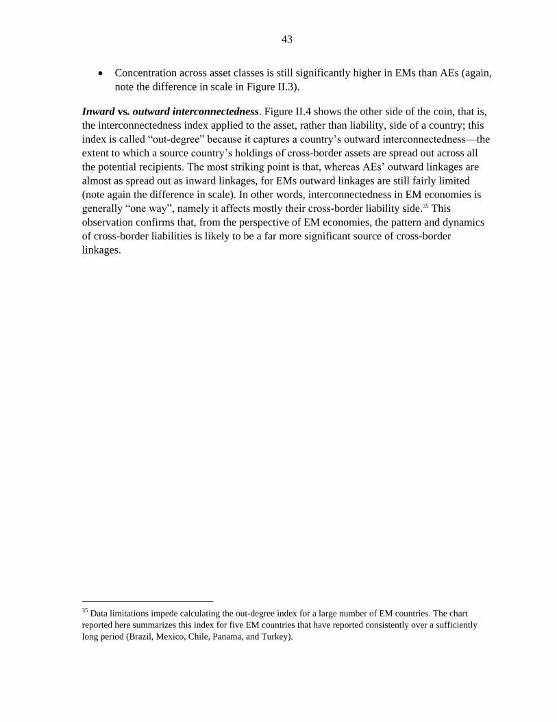
43
Concentration across asset classes is still significantly higher in EMs than AEs (again,
note the difference in scale in Figure II.3).
Inward vs. outward interconnectedness. Figure II.4 shows the other side of the coin, that is,
the interconnectedness index applied to the asset, rather than liability, side of a country; this
index is called ―out-degree‖ because it captures a country‘s outward interconnectedness—the
extent to which a source country‘s holdings of cross-border assets are spread out across all
the potential recipients. The most striking point is that, whereas AEs‘ outward linkages are
almost as spread out as inward linkages, for EMs outward linkages are still fairly limited
(note again the difference in scale). In other words, interconnectedness in EM economies is
generally ―one way‖, namely it affects mostly their cross-border liability side.35 This
observation confirms that, from the perspective of EM economies, the pattern and dynamics
of cross-border liabilities is likely to be a far more significant source of cross-border
linkages.
35 Data limitations impede calculating the out-degree index for a large number of EM countries. The chart
reported here summarizes this index for five EM countries that have reported consistently over a sufficiently
long period (Brazil, Mexico, Chile, Panama, and Turkey).
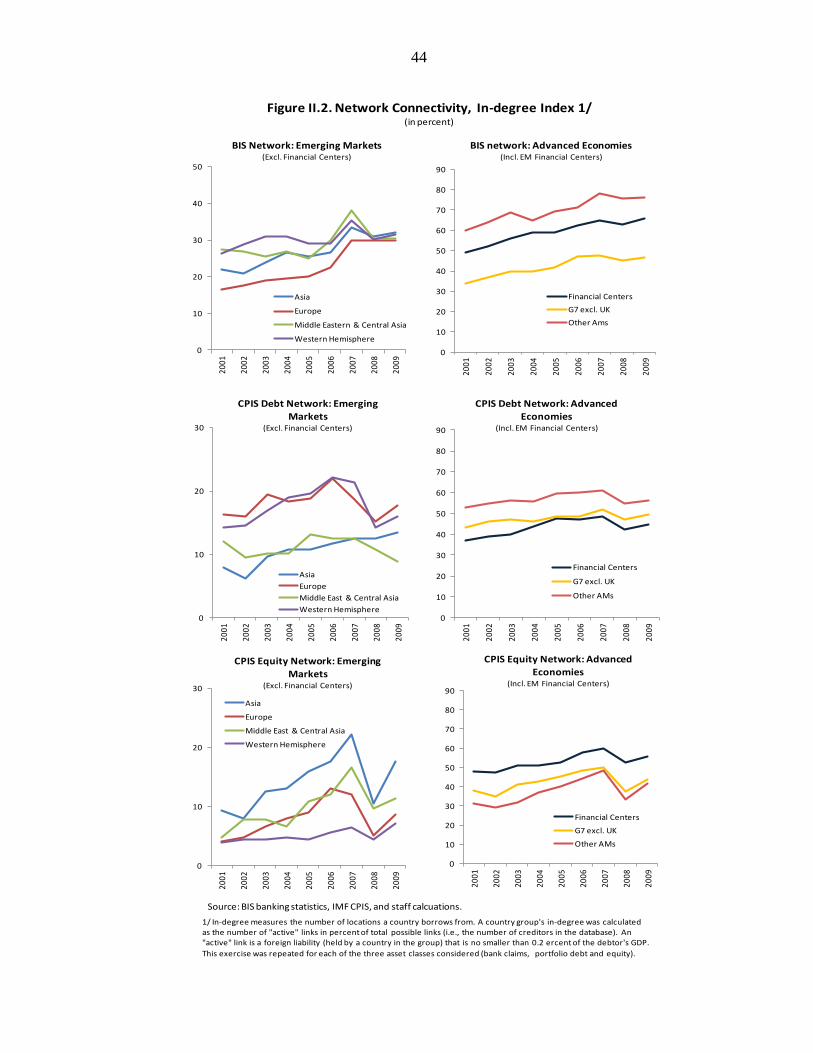
44
Figure II.2. Network Connectivity, In-degree Index 1/(in percent)
Source: BIS banking statistics, IMF CPIS, and staff calcuations.
0
10
20
30
40
50
2001
2002
2003
2004
2005
2006
2007
2008
2009
BIS Network: Emerging Markets (Excl. Financial Centers)
Asia
Europe
Middle Eastern & Central Asia
Western Hemisphere
0
10
20
30
40
50
60
70
80
90
2001
2002
2003
2004
2005
2006
2007
2008
2009
BIS network: Advanced Economies(Incl. EM Financial Centers)
Financial Centers
G7 excl. UK
Other Ams
0
10
20
30
2001
2002
2003
2004
2005
2006
2007
2008
2009
CPIS Debt Network: Emerging Markets
(Excl. Financial Centers)
Asia
Europe
Middle East & Central Asia
Western Hemisphere0
10
20
30
40
50
60
70
80
90
2001
2002
2003
2004
2005
2006
2007
2008
2009
CPIS Debt Network: Advanced Economies
(Incl. EM Financial Centers)
Financial Centers
G7 excl. UK
Other AMs
0
10
20
30
2001
2002
2003
2004
2005
2006
2007
2008
2009
CPIS Equity Network: Emerging
Markets(Excl. Financial Centers)
Asia
Europe
Middle East & Central Asia
Western Hemisphere
0
10
20
30
40
50
60
70
80
90
2001
2002
2003
2004
2005
2006
2007
2008
2009
CPIS Equity Network: Advanced
Economies(Incl. EM Financial Centers)
Financial Centers
G7 excl. UK
Other AMs
1/ In-degree measures the number of locations a country borrows from. A country group's in-degree was calculated as the number of "active" links in percent of total possible links (i.e., the number of creditors in the database). An "active" link is a foreign liability (held by a country in the group) that is no smaller than 0.2 ercent of the debtor's GDP.
This exercise was repeated for each of the three asset classes considered (bank claims, portfolio debt and equity).
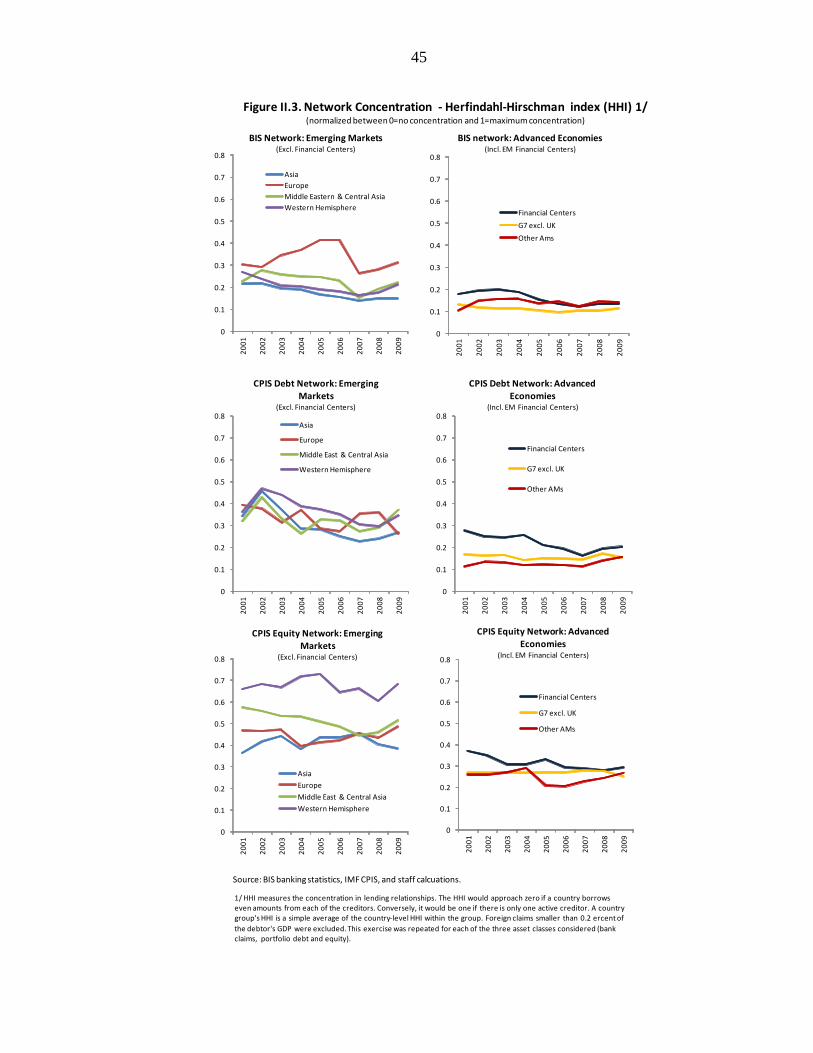
45
Figure II.3. Network Concentration - Herfindahl-Hirschman index (HHI) 1/(normalized between 0=no concentration and 1=maximum concentration)
Source: BIS banking statistics, IMF CPIS, and staff calcuations.
0
0.1
0.2
0.3
0.4
0.5
0.6
0.7
0.8
20
01
20
02
20
03
20
04
20
05
20
06
20
07
20
08
20
09
BIS Network: Emerging Markets (Excl. Financial Centers)
Asia
Europe
Middle Eastern & Central Asia
Western Hemisphere
0
0.1
0.2
0.3
0.4
0.5
0.6
0.7
0.8
20
01
20
02
20
03
20
04
20
05
20
06
20
07
20
08
20
09
BIS network: Advanced Economies(Incl. EM Financial Centers)
Financial Centers
G7 excl. UK
Other Ams
0
0.1
0.2
0.3
0.4
0.5
0.6
0.7
0.8
20
01
20
02
20
03
20
04
20
05
20
06
20
07
20
08
20
09
CPIS Debt Network: Emerging
Markets(Excl. Financial Centers)
Asia
Europe
Middle East & Central Asia
Western Hemisphere
0
0.1
0.2
0.3
0.4
0.5
0.6
0.7
0.8
20
01
20
02
20
03
20
04
20
05
20
06
20
07
20
08
20
09
CPIS Debt Network: Advanced
Economies(Incl. EM Financial Centers)
Financial Centers
G7 excl. UK
Other AMs
0
0.1
0.2
0.3
0.4
0.5
0.6
0.7
0.8
20
01
20
02
20
03
20
04
20
05
20
06
20
07
20
08
20
09
CPIS Equity Network: Emerging Markets
(Excl. Financial Centers)
Asia
Europe
Middle East & Central Asia
Western Hemisphere
0
0.1
0.2
0.3
0.4
0.5
0.6
0.7
0.8
20
01
20
02
20
03
20
04
20
05
20
06
20
07
20
08
20
09
CPIS Equity Network: Advanced Economies
(Incl. EM Financial Centers)
Financial Centers
G7 excl. UK
Other AMs
1/ HHI measures the concentration in lending relationships. The HHI would approach zero if a country borrows even amounts from each of the creditors. Conversely, it would be one if there is only one active creditor. A country group's HHI is a simple average of the country-level HHI within the group. Foreign claims smaller than 0.2 ercent of
the debtor's GDP were excluded. This exercise was repeated for each of the three asset classes considered (bank claims, portfolio debt and equity).
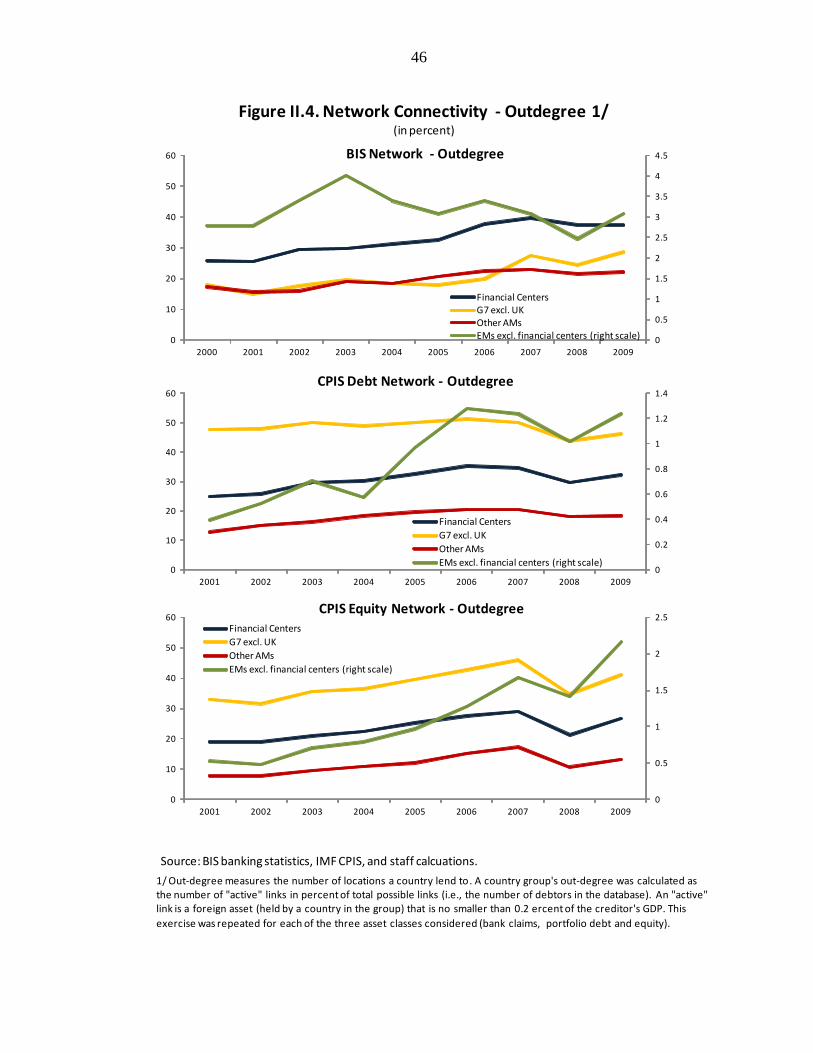
46
Herfindahl index
Figure II.4. Network Connectivity - Outdegree 1/(in percent)
Source: BIS banking statistics, IMF CPIS, and staff calcuations.
0
0.5
1
1.5
2
2.5
3
3.5
4
4.5
0
10
20
30
40
50
60
2000 2001 2002 2003 2004 2005 2006 2007 2008 2009
BIS Network - Outdegree
Financial CentersG7 excl. UKOther AMsEMs excl. financial centers (right scale)
0
0.2
0.4
0.6
0.8
1
1.2
1.4
0
10
20
30
40
50
60
2001 2002 2003 2004 2005 2006 2007 2008 2009
CPIS Debt Network - Outdegree
Financial Centers
G7 excl. UK
Other AMs
EMs excl. financial centers (right scale)
0
0.5
1
1.5
2
2.5
0
10
20
30
40
50
60
2001 2002 2003 2004 2005 2006 2007 2008 2009
CPIS Equity Network - Outdegree Financial Centers
G7 excl. UK
Other AMs
EMs excl. financial centers (right scale)
1/ Out-degree measures the number of locations a country lend to. A country group's out-degree was calculated as the number of "active" links in percent of total possible links (i.e., the number of debtors in the database). An "active"link is a foreign asset (held by a country in the group) that is no smaller than 0.2 ercent of the creditor's GDP. This
exercise was repeated for each of the three asset classes considered (bank claims, portfolio debt and equity).
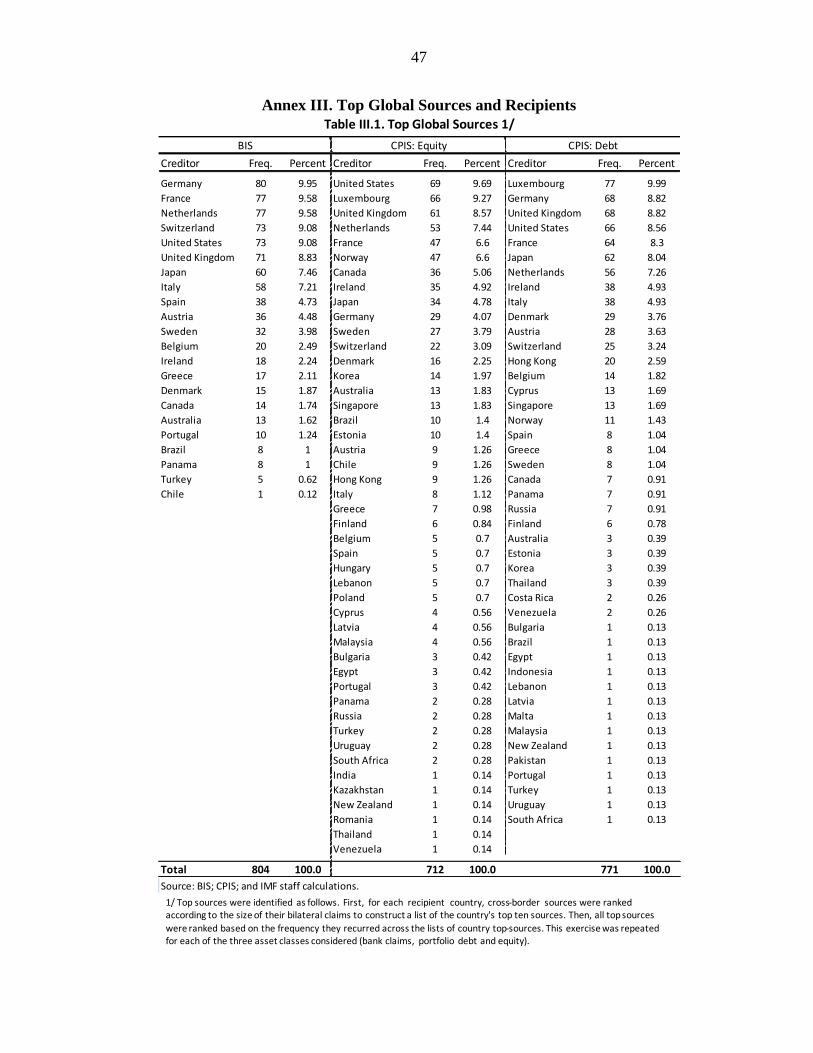
47
Annex III. Top Global Sources and Recipients
Creditor Freq. Percent Creditor Freq. Percent Creditor Freq. Percent
Germany 80 9.95 United States 69 9.69 Luxembourg 77 9.99
France 77 9.58 Luxembourg 66 9.27 Germany 68 8.82
Netherlands 77 9.58 United Kingdom 61 8.57 United Kingdom 68 8.82
Switzerland 73 9.08 Netherlands 53 7.44 United States 66 8.56
United States 73 9.08 France 47 6.6 France 64 8.3
United Kingdom 71 8.83 Norway 47 6.6 Japan 62 8.04
Japan 60 7.46 Canada 36 5.06 Netherlands 56 7.26
Italy 58 7.21 Ireland 35 4.92 Ireland 38 4.93
Spain 38 4.73 Japan 34 4.78 Italy 38 4.93
Austria 36 4.48 Germany 29 4.07 Denmark 29 3.76
Sweden 32 3.98 Sweden 27 3.79 Austria 28 3.63
Belgium 20 2.49 Switzerland 22 3.09 Switzerland 25 3.24
Ireland 18 2.24 Denmark 16 2.25 Hong Kong 20 2.59
Greece 17 2.11 Korea 14 1.97 Belgium 14 1.82
Denmark 15 1.87 Australia 13 1.83 Cyprus 13 1.69
Canada 14 1.74 Singapore 13 1.83 Singapore 13 1.69
Australia 13 1.62 Brazil 10 1.4 Norway 11 1.43
Portugal 10 1.24 Estonia 10 1.4 Spain 8 1.04
Brazil 8 1 Austria 9 1.26 Greece 8 1.04
Panama 8 1 Chile 9 1.26 Sweden 8 1.04
Turkey 5 0.62 Hong Kong 9 1.26 Canada 7 0.91
Chile 1 0.12 Italy 8 1.12 Panama 7 0.91
Greece 7 0.98 Russia 7 0.91
Finland 6 0.84 Finland 6 0.78
Belgium 5 0.7 Australia 3 0.39
Spain 5 0.7 Estonia 3 0.39
Hungary 5 0.7 Korea 3 0.39
Lebanon 5 0.7 Thailand 3 0.39
Poland 5 0.7 Costa Rica 2 0.26
Cyprus 4 0.56 Venezuela 2 0.26
Latvia 4 0.56 Bulgaria 1 0.13
Malaysia 4 0.56 Brazil 1 0.13
Bulgaria 3 0.42 Egypt 1 0.13
Egypt 3 0.42 Indonesia 1 0.13
Portugal 3 0.42 Lebanon 1 0.13
Panama 2 0.28 Latvia 1 0.13
Russia 2 0.28 Malta 1 0.13
Turkey 2 0.28 Malaysia 1 0.13
Uruguay 2 0.28 New Zealand 1 0.13
South Africa 2 0.28 Pakistan 1 0.13
India 1 0.14 Portugal 1 0.13
Kazakhstan 1 0.14 Turkey 1 0.13
New Zealand 1 0.14 Uruguay 1 0.13
Romania 1 0.14 South Africa 1 0.13
Thailand 1 0.14
Venezuela 1 0.14
Total 804 100.0 712 100.0 771 100.0
Source: BIS; CPIS; and IMF staff calculations.
Table III.1. Top Global Sources 1/
BIS CPIS: Equity CPIS: Debt
1/ Top sources were identified as follows. First, for each recipient country, cross-border sources were ranked according to the size of their bilateral claims to construct a list of the country's top ten sources. Then, all top sources
were ranked based on the frequency they recurred across the lists of country top-sources. This exercise was repeated for each of the three asset classes considered (bank claims, portfolio debt and equity).
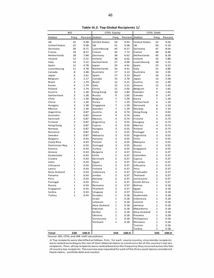
48
Debtor Freq. Percent Debtor Freq. Percent Debtor Freq. Percent
UK 22 9.58 United States 54 9.93 United States 52 9.56
United States 22 9.58 UK 51 9.38 UK 50 9.19
Germany 20 8.71 Luxembourg 45 8.27 Germany 47 8.64
France 19 8.27 France 42 7.72 France 46 8.46
Netherlands 18 7.84 Germany 36 6.62 Netherlands 45 8.28
Ireland 12 5.22 Ireland 36 6.62 Ireland 32 5.88
Italy 12 5.22 Switzerland 27 4.96 Luxembourg 28 5.15
Spain 11 4.78 Japan 24 4.41 Spain 23 4.23
Luxembourg 11 4.78 Netherlands 24 4.41 Italy 21 3.86
Canada 8 3.48 Australia 17 3.13 Australia 16 2.95
Japan 6 2.61 Spain 17 3.13 Brazil 16 2.95
Belgium 5 2.17 Canada 15 2.76 Japan 14 2.58
Brazil 4 1.74 Brazil 12 2.21 Austria 13 2.40
Korea 4 1.74 Italy 12 2.21 Greece 12 2.20
Poland 4 1.74 China 11 2.02 Belgium 9 1.65
Austria 3 1.30 Hong Kong 10 1.84 Sweden 9 1.65
Switzerland 3 1.30 Russia 9 1.65 Canada 8 1.47
Chile 3 1.30 Belgium 7 1.29 Korea 7 1.28
China 3 1.30 Korea 7 1.29 Switzerland 6 1.10
Hungary 3 1.30 Singapore 7 1.29 Denmark 6 1.10
Mexico 3 1.30 Sweden 7 1.29 Norway 6 1.10
Argentina 2 0.87 Austria 4 0.74 Hong Kong 5 0.92
Australia 2 0.87 Greece 4 0.74 India 5 0.92
Denmark 2 0.87 Mexico 4 0.74 Finland 4 0.73
Finland 2 0.87 Argentina 3 0.55 Hungary 4 0.73
Hong Kong 2 0.87 Cyprus 3 0.55 Mexico 4 0.73
Norway 2 0.87 Hungary 3 0.55 Poland 4 0.73
Romania 2 0.87 India 3 0.55 Portugal 4 0.73
Sweden 2 0.87 Malaysia 3 0.55 Argentina 3 0.55
Bulgaria 1 0.43 Panama 3 0.55 Chile 3 0.55
Costa Rica 1 0.43 Poland 3 0.55 Malaysia 3 0.55
Dominican Rep. 1 0.43 Portugal 3 0.55 Russia 3 0.55
Estonia 1 0.43 Turkey 3 0.55 Singapore 3 0.55
Greece 1 0.43 Bulgaria 2 0.37 China 2 0.37
Guatemala 1 0.43 Chile 2 0.37 Colombia 2 0.37
Croatia 1 0.43 Denmark 2 0.37 Cyprus 2 0.37
India 1 0.43 Egypt 2 0.37 Sri Lanka 2 0.37
Lithuania 1 0.43 Estonia 2 0.37 Lithuania 2 0.37
Latvia 1 0.43 Finland 2 0.37 Peru 2 0.37
New Zealand 1 0.43 Indonesia 2 0.37 El Salvador 2 0.37
Panama 1 0.43 Jordan 2 0.37 Thailand 2 0.37
Peru 1 0.43 Norway 2 0.37 Venezuela 2 0.37
Portugal 1 0.43 Peru 2 0.37 South Africa 2 0.37
Russia 1 0.43 Romania 2 0.37 Bolivia 1 0.18
Singapore 1 0.43 Thailand 2 0.37 Egypt 1 0.18
Serbia 1 0.43 Uruguay 2 0.37 Estonia 1 0.18
Turkey 1 0.43 Ecuador 1 0.18 Guatemala 1 0.18
Israel 1 0.18 Indonesia 1 0.18
Lebanon 1 0.18 Iceland 1 0.18
New Zealand 1 0.18 Jamaica 1 0.18
Pakistan 1 0.18 Macedonia 1 0.18
Serbia 1 0.18 New Zealand 1 0.18
Ukraine 1 0.18 Panama 1 0.18
Venezuela 1 0.18 Philippines 1 0.18
Vietnam 1 0.18 Romania 1 0.18
Tunisia 1 0.18
Turkey 1 0.18
Total 230 100.0 544 100.0 545 100.0
Source: BIS; CPIS; and IMF staff calculations.
BIS CPIS: Equity CPIS: Debt
Table III.2. Top Global Recipients 1/
1/ Top recipients were identified as follows. First, for each source country, cross-border recipients were ranked according to the size of their bilateral claims to construct a list of the country's top ten recipients. Then, all top recipients were ranked based on the frequency they recurred across the lists of country top-recipients. This exercise was repeated for each of the three asset classes considered (bank claims, portfolio debt and equity).
49
Annex IV. Importance of Global Factors in Driving Capital Inflows to EMs36
This annex investigates the quantitative importance of global factors and country-specific
fundamentals in driving cross-border capital inflows to EMs. The conservative estimates
discussed below suggest that global factors could explain at least 25 percent of variations in
total gross inflows; for portfolio inflows, however, global factors are likely much more
important (above 50 percent). Moreover, the relative importance of global factors is likely to
shift over time, reflecting in particular global financial and liquidity conditions.
These shares were calculated using the same panel framework as in IMF, 2011e, which
included both global and domestic variables as determinants of capital inflows. One problem
in computing the contribution of global factors in this framework is that the overall variance
of inflows (in log levels) in a panel of 48 EMs is largely driven by cross-country variation of
inflows. The latter is often a result of country specific factors (e.g. political conditions or
idiosyncratic developments such as privatization or lumpy investment projects) that are likely
to drive capital flows without being directly linked to differences in domestic
macroeconomic conditions—that is, the domestic pull factors that one would like to isolate
here.37 To correct for this potential bias, the total variance of underlying flows was broken
down into two components, variance across countries and over time. The contribution of
global factors was then computed as the ratio of their variance to the variance of gross capital
inflows over time.
In this framework, global factors (U.S. long term interest rates and the VIX risk index)
explained on average around 25 percent of the cross-time variation of gross total capital
inflows to EMs; for portfolio inflows, the estimated share rose to 54 percent. These shares
were computed by treating domestic variables as completely unaffected by global variables,
while in practice they are likely to be influenced by the latter. When domestic variables were
omitted from the estimated regressions, the share of cross-time variation explained by global
factor rose to 65 and 87 percent, respectively, for total and portfolio inflows—an indirect
sign that domestic variables are indeed affected significantly by global factors. These
estimates can be thought of as an upper bound for the role of global factors for capital
inflows.
36 Prepared by Yanliang Miao.
37 Using outright variance decomposition from panel regressions, the variance of global factors accounts for a
mere 5 percent of total sample variation. This estimate is likely to have a significant downward bias, however,
for the reason discussed in the text.
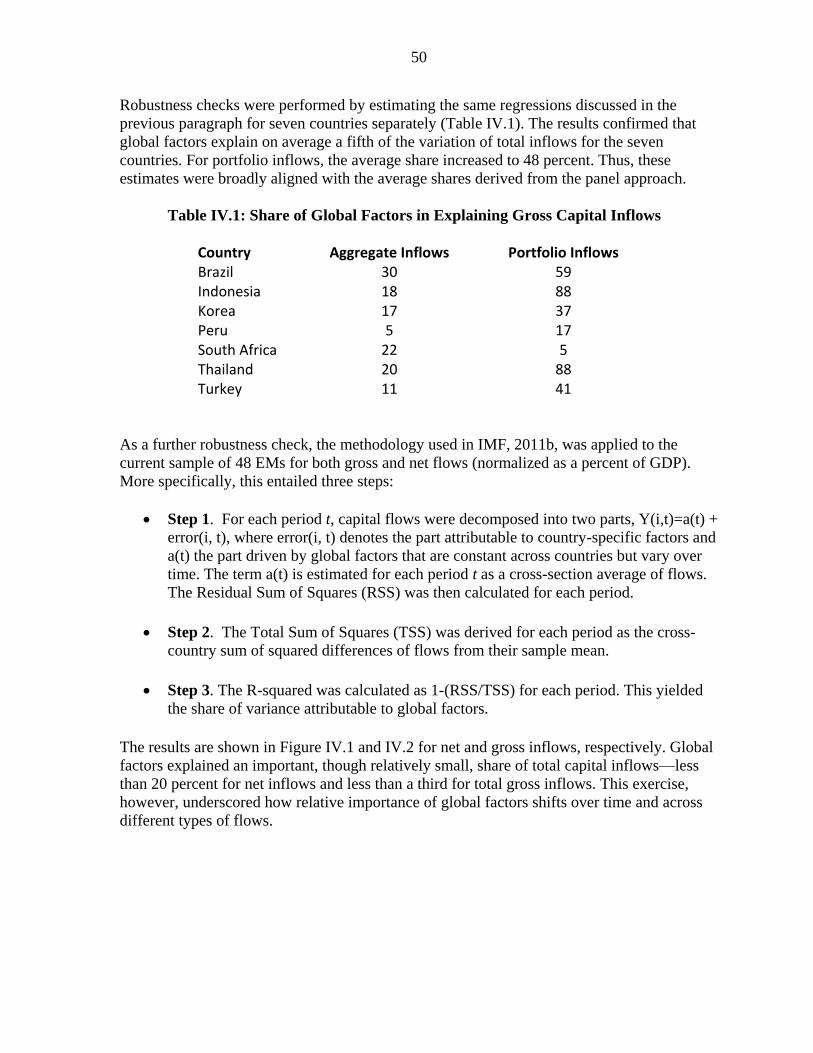
50
Robustness checks were performed by estimating the same regressions discussed in the
previous paragraph for seven countries separately (Table IV.1). The results confirmed that
global factors explain on average a fifth of the variation of total inflows for the seven
countries. For portfolio inflows, the average share increased to 48 percent. Thus, these
estimates were broadly aligned with the average shares derived from the panel approach.
Table IV.1: Share of Global Factors in Explaining Gross Capital Inflows
Country Aggregate Inflows Portfolio Inflows Brazil 30 59 Indonesia 18 88 Korea 17 37 Peru 5 17 South Africa 22 5 Thailand 20 88 Turkey 11 41
As a further robustness check, the methodology used in IMF, 2011b, was applied to the
current sample of 48 EMs for both gross and net flows (normalized as a percent of GDP).
More specifically, this entailed three steps:
Step 1. For each period t, capital flows were decomposed into two parts, Y(i,t)=a(t) +
error(i, t), where error(i, t) denotes the part attributable to country-specific factors and
a(t) the part driven by global factors that are constant across countries but vary over
time. The term a(t) is estimated for each period t as a cross-section average of flows.
The Residual Sum of Squares (RSS) was then calculated for each period.
Step 2. The Total Sum of Squares (TSS) was derived for each period as the cross-
country sum of squared differences of flows from their sample mean.
Step 3. The R-squared was calculated as 1-(RSS/TSS) for each period. This yielded
the share of variance attributable to global factors.
The results are shown in Figure IV.1 and IV.2 for net and gross inflows, respectively. Global
factors explained an important, though relatively small, share of total capital inflows—less
than 20 percent for net inflows and less than a third for total gross inflows. This exercise,
however, underscored how relative importance of global factors shifts over time and across
different types of flows.
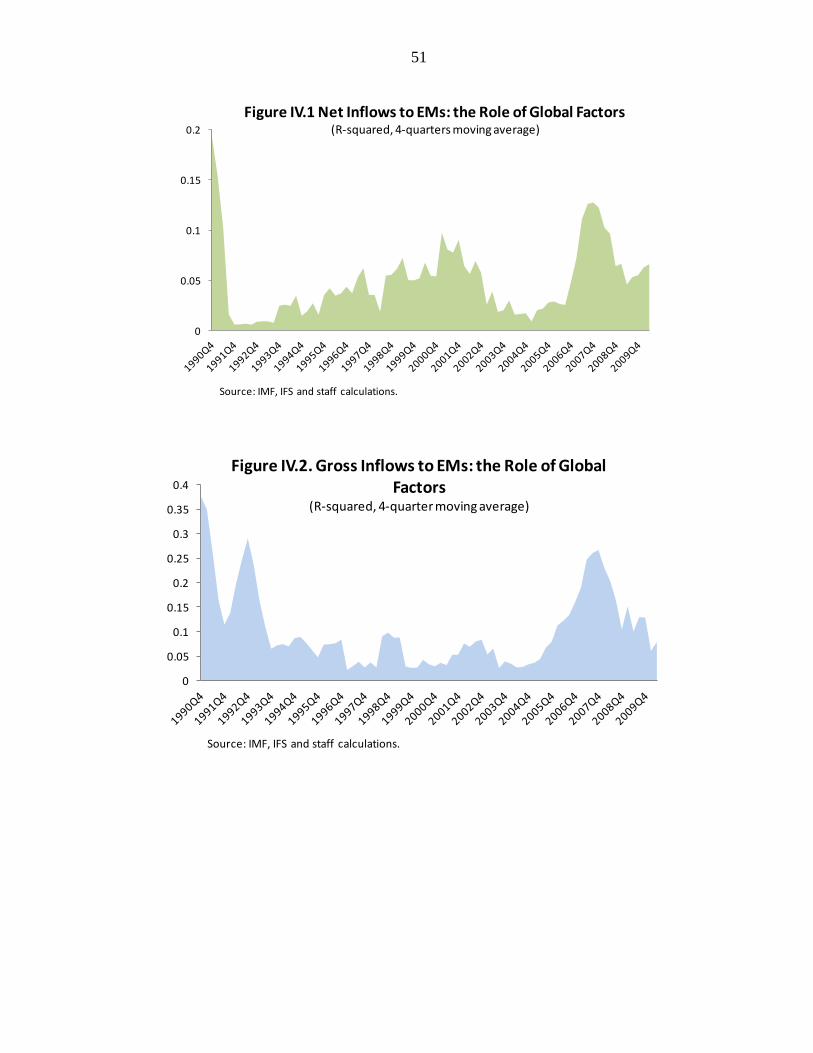
51
0
0.05
0.1
0.15
0.2
Figure IV.1 Net Inflows to EMs: the Role of Global Factors (R-squared, 4-quarters moving average)
Source: IMF, IFS and staff calculations.
0
0.05
0.1
0.15
0.2
0.25
0.3
0.35
0.4
Figure IV.2. Gross Inflows to EMs: the Role of Global Factors
(R-squared, 4-quarter moving average)
Source: IMF, IFS and staff calculations.
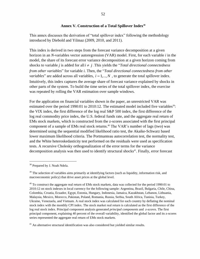
52
Annex V. Construction of a Total Spillover Index38
This annex discusses the derivation of ―total spillover index‖ following the methodology
introduced by Diebold and Yilmaz (2009, 2010, and 2011).
This index is derived in two steps from the forecast variance decomposition at a given
horizon in an N-variables vector autoregression (VAR) model. First, for each variable i in the
model, the share of its forecast error variance decomposition at a given horizon coming from
shocks to variable j is added for all ji . This yields the ―Total directional connectedness
from other variables‖ for variable i. Then, the ―Total directional connectedness from other
variables‖ are added across all variables, Ni ,...,1 , to generate the total spillover index.
Intuitively, this index captures the average share of forecast variance explained by shocks in
other parts of the system. To build the time series of the total spillover index, the exercise
was repeated by rolling the VAR estimation over sample windows.
For the application on financial variables shown in the paper, an unrestricted VAR was
estimated over the period 1990:01 to 2010:12. The estimated model included five variables39:
the VIX index, the first difference of the log real S&P 500 index, the first difference of the
log real commodity price index, the U.S. federal funds rate, and the aggregate real return of
EMs stock markets, which is constructed from the z-scores associated with the first principal
component of a sample of EMs real stock returns.40 The VAR‘s number of lags (two) was
determined using the sequential modified likelihood ratio test, the Akaike-Schwarz based
lower maximum likelihood criteria. The Portmanteau autocorrelation test, the normality test,
and the White heteroskedasticity test performed on the residuals were used as specification
tests. A recursive Cholesky orthogonalization of the error terms for the variance
decomposition analysis was then used to identify structural shocks41. Finally, error forecast
38 Prepared by J. Noah Ndela.
39 The selection of variables aims primarily at identifying factors (such as liquidity, information risk, and
macroeconomic policy) that drive asset prices at the global level.
40 To construct the aggregate real return of EMs stock markets, data was collected for the period 1990:01 to
2010:12 on stock indexes in local currency for the following sample: Argentina, Brazil, Bulgaria, Chile, China,
Colombia, Croatia, Ecuador, Egypt, Estonia, Hungary, Indonesia, Jamaica, Kazakhstan, Lebanon, Lithuania,
Malaysia, Mexico, Morocco, Pakistan, Poland, Romania, Russia, Serbia, South Africa, Tunisia, Turkey,
Ukraine, Venezuela, and Vietnam. A real stock index was calculated for each country by deflating the nominal
stock index with the monthly CPI index. The stock market real return is calculated as the first difference of the
log real stock index. Principal component analysis generated principal components and z-scores. The first
principal component, explaining 40 percent of the overall variability, identified the global factor and its z-scores
series represented the aggregate real return of EMs stock markets.
41 An alternative structural identification was also considered but yielded similar results.
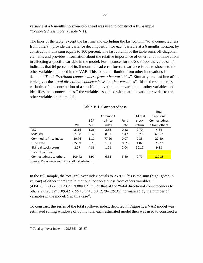
53
variance at a 6 months horizon-step ahead was used to construct a full-sample
―Connectedness table‖ (Table V.1).
The lines of the table (except the last line and excluding the last column ―total connectedness
from others‖) provide the variance decomposition for each variable at a 6 months horizon; by
construction, this sum equals to 100 percent. The last column of the table sums off-diagonal
elements and provides information about the relative importance of other random innovations
in affecting a specific variable in the model. For instance, for the S&P 500, the value of 64
indicates that 64 percent of its 6-month-ahead error forecast variance is due to shocks to the
other variables included in the VAR. This total contribution from other innovations is
denoted ―Total directional connectedness from other variables‖. Similarly, the last line of the
table gives the ―total directional connectedness to other variables‖; this is the sum across
variables of the contribution of a specific innovation to the variation of other variables and
identifies the ―connectedness‖ the variable associated with that innovation provides to the
other variables in the model.
Table V.1. Connectedness
VIX
S&P
500
Commodit
y Price
Index
Fund
Rate
EM real
stock
return
Total
directional
Connectednes
s from others
VIX 95.16 1.26 2.66 0.22 0.70 4.84
S&P 500 61.00 36.43 0.87 1.47 0.23 63.57
Commodity Price Index 20.76 1.11 77.20 0.07 0.85 22.80
Fund Rate 25.39 0.25 1.61 71.73 1.02 28.27
EM real stock return 2.27 4.36 1.21 2.04 90.12 9.88
Total directional
Connectedness to others 109.42 6.99 6.35 3.80 2.79 129.35
Source: Datastream and IMF staff calculations.
In the full sample, the total spillover index equals to 25.87. This is the sum (highlighted in
yellow) of either the ―Total directional connectedness from others variables‖
(4.84+63.57+22.80+28.27+9.88=129.35) or that of the ―total directional connectedness to
others variables‖ (109.42+6.99+6.35+3.80+2.79=129.35) normalized by the number of
variables in the model, 5 in this case42.
To construct the series of the total spillover index, depicted in Figure 1, a VAR model was
estimated rolling windows of 60 months; each estimated model then was used to construct a
42 Total spillover index = 129.35/5 = 25.87
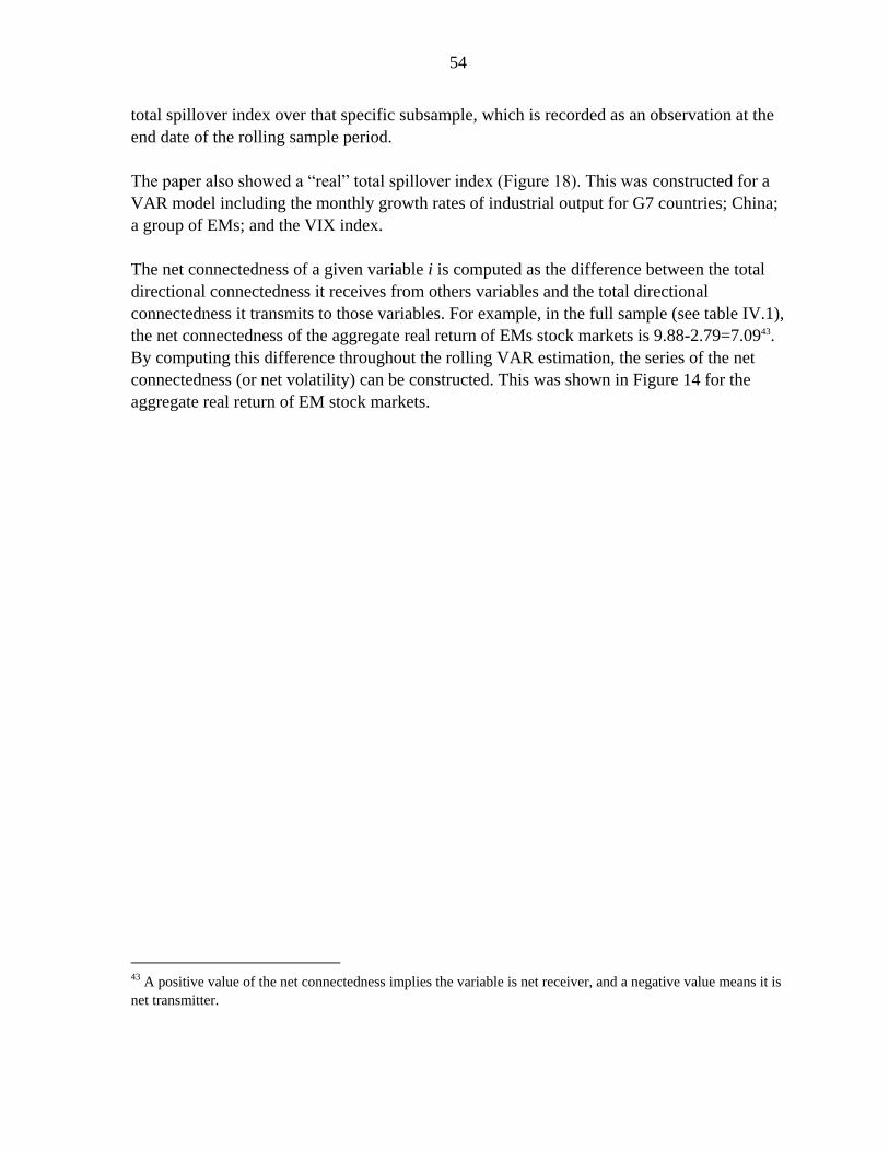
54
total spillover index over that specific subsample, which is recorded as an observation at the
end date of the rolling sample period.
The paper also showed a ―real‖ total spillover index (Figure 18). This was constructed for a
VAR model including the monthly growth rates of industrial output for G7 countries; China;
a group of EMs; and the VIX index.
The net connectedness of a given variable i is computed as the difference between the total
directional connectedness it receives from others variables and the total directional
connectedness it transmits to those variables. For example, in the full sample (see table IV.1),
the net connectedness of the aggregate real return of EMs stock markets is 9.88-2.79=7.0943.
By computing this difference throughout the rolling VAR estimation, the series of the net
connectedness (or net volatility) can be constructed. This was shown in Figure 14 for the
aggregate real return of EM stock markets.
43 A positive value of the net connectedness implies the variable is net receiver, and a negative value means it is
net transmitter.
55
Annex VI. Evidence from Cross-Border Banking Groups44
This annex first describes the construction of the underlying dataset used in the analysis of
the behavior of cross-border banking groups and then summarizes the empirical results
discussed in the paper. The focus of the analysis was on the operations of commercial
banking groups; this analysis thus complements previous staff work on financial
interconnectedness from the perspective of Large Complex Financial Institutions (IMF, 2010c).
Construction of Banking Groups
As described in Porter and Serra, 2011, one of the main contributions of this exercise was to
construct a novel dataset on cross-border banking groups. This dataset covers the ownership
structure of every banking/financial group with at least one foreign subsidiary between 1995
and 2009 on an ultimate ownership basis.45 The dataset was built starting from ownership and
subsidiary data available in Bankscope since 2002, and then by extending it back to 1995
using the information provided in Bankers‘ Almanac as well as resorting to parent banks‘
annual reports, working papers on foreign banking activity, and handbooks of banking
history. The final ownership dataset included a matching of every ultimate owner to its
domestic and foreign subsidiaries, and the ultimate owner‘s home country and shareholdings
between 1995 and 2009. Balance sheet data and financial soundness indicators, as well as
macroeconomic and financial data, were matched to subsidiaries and parent banks using
Bankscope and Bloomberg, respectively.
Ownership and Diversification Patters
With the individual banking group structures established, it was possible to describe the
importance of cross-border banking groups in EMs, as well as describe their group-level
structure and diversification.
The importance of cross-border banks in EMs was calculated using these banks‘
assets in percent of the assets for all banks in the domestic banking system.
The diversification of banking groups was calculated using the Herfindahl-Hirschman
index (HHI) (see Annex II). This provided an index of group concentration across
44 Prepared by Nathan Porter and Cesar Serra.
45 The term subsidiary is used here to also include branch data reported in Bankscope. Using ultimate ownership
basis allowed avoiding spurious testing by not using the direct ownership structure reported by parent banks,
which commonly set aside a different subsidiary outside the home country or an acquired foreign bank to be a
holding or manage other foreign subsidiary.
56
locations. This was calculated separately for all subsidiary locations (including
domestic ones) as well as for only those subsidiaries outside the parent country.
The geographic span of a banking group was measured by the average distance of
group assets from the parent country. This was calculated as the average distance of
each subsidiary location in kilometers, weighted by the assets of that subsidiary.
Regression Analysis
Panel regression analysis of subsidiaries-parent links was used to understand the potential
channels through which shocks affecting parent banks spill over to their subsidiaries.46 Given
the relatively minor role EM parents play in EM banking sectors, the analysis was focused on
links that involve AM parents and subsidiaries in EMs. The estimated relationship aimed to
explain subsidiary-level new lending (relative to subsidiary assets) through both local and
parent-country (and global) macroeconomic factors, as well as the financial soundness of
both the parent and subsidiary. Financial soundness was captured through solvency (capital
adequacy and the volatility of the parent‘s equity price), leverage (equity/assets), liquidity
(liquid assets/assets), credit quality (nonperforming loan ratio), and profitability (return on
equity). Local macroeconomic conditions were controlled for with the inclusion of local
GDP growth and the appreciation of the bilateral US$ exchange rate, while parental and
global macroeconomic conditions were controlled for with the parent country growth and the
VIX index. To overcome their potential endogeneity, all the bank-specific variables were
lagged.
The financial conditions of both the parent and subsidiary significantly were found to affect
new lending (Table VI.1). Excessive leverage (low equity-to-assets), and low liquidity, in the
local subsidiary significantly reduce the ability of that subsidiary to extend new loans.
However, recent local profitably has at most a marginal impact on lending. Importantly,
however, parental liquidity and capital adequacy also significantly affect the ability of the
bank to extend loans, with parental profitability again marginally important. Lower parental
liquidity inhibits the ability of subsidiaries to extend new loans, suggesting an important
channel for liquidity shocks. This could operate through the ability of the local bank to
borrow from the parent, or the need for the parent to borrow from the subsidiary (in line with
Cetorelli and Goldberg, 2010), higher counter-party concerns in the local interbank market
affecting access of the subsidiary, or even the within-group currency mismatches (Fender and
McGuire, 2010). Stronger parental capital adequacy is associated with lower subsidiary
lending. This may reflect the fact that, conditional on a healthy subsidiary (high liquidity and
low leverage), a parent with a stronger capital may be able to lend separately into the local
46 Subsidiaries are defined as foreign affiliates owned with at least 50 percent shareholding by a banking group.
The results on the regressions were robust to an an alternative cutoff of at least 40 percent shareholding, with no
other shareholder owning more than 40 percent.
57
market, or withdraw capital from the local subsidiary conditionally affecting local lending.
While significant, the empirical impact of this is, nonetheless, small. Macroeconomic
conditions and aggregate volatility are also both important for subsidiary lending, with higher
local and parental growth and lower aggregate volatility associated with more new lending.
Figure 17 in the paper summarizes these results. Aggregating these potential channels
highlights the importance of the health of the subsidiary, but also suggests important liquidity
connections between parent and subsidiary banks. Shocks that raise local growth or change
the financial conditions of the subsidiary from the 25th
to the 75th
percentile of the
distribution increase new lending by 80 percent or 124 percent of its median value,
respectively. Shocks of similar magnitude that strengthen the financial conditions of the
parent bank raise lending in 35 percent, reflecting the importance of improved parental
liquidity.
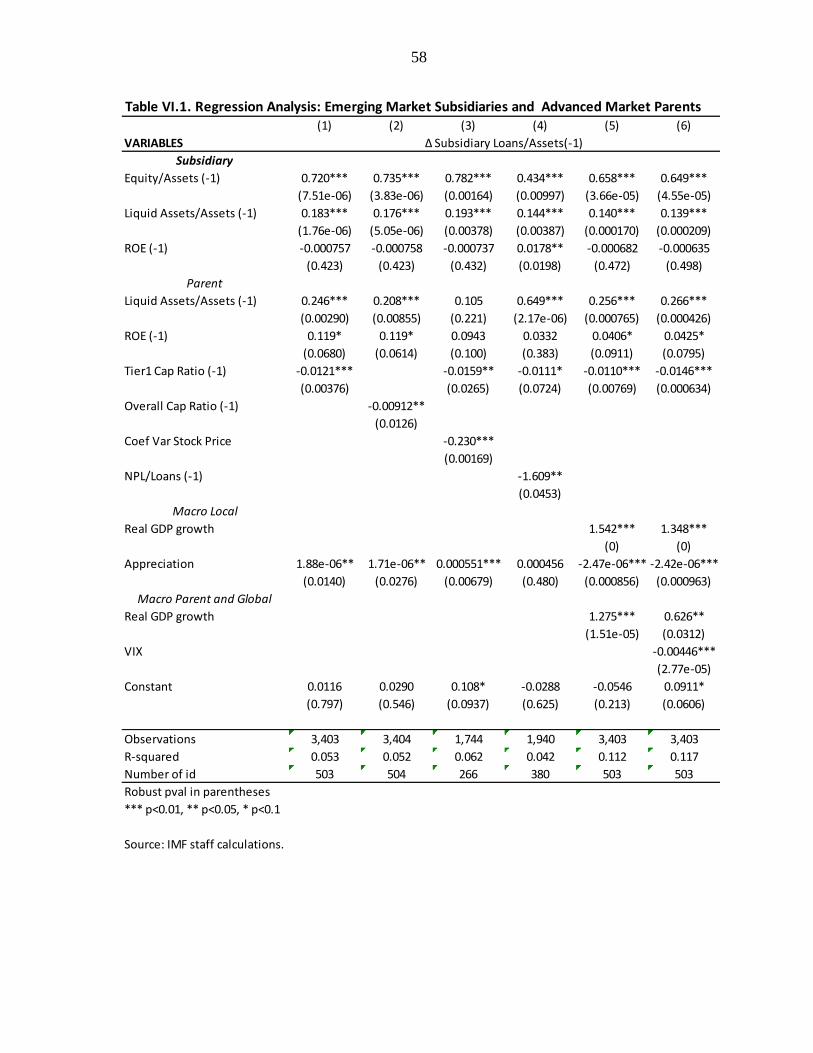
58
Table VI.1. Regression Analysis: Emerging Market Subsidiaries and Advanced Market Parents(1) (2) (3) (4) (5) (6)
VARIABLES
Subsidiary
Equity/Assets (-1) 0.720*** 0.735*** 0.782*** 0.434*** 0.658*** 0.649***
(7.51e-06) (3.83e-06) (0.00164) (0.00997) (3.66e-05) (4.55e-05)
Liquid Assets/Assets (-1) 0.183*** 0.176*** 0.193*** 0.144*** 0.140*** 0.139***
(1.76e-06) (5.05e-06) (0.00378) (0.00387) (0.000170) (0.000209)
ROE (-1) -0.000757 -0.000758 -0.000737 0.0178** -0.000682 -0.000635
(0.423) (0.423) (0.432) (0.0198) (0.472) (0.498)
Parent
Liquid Assets/Assets (-1) 0.246*** 0.208*** 0.105 0.649*** 0.256*** 0.266***
(0.00290) (0.00855) (0.221) (2.17e-06) (0.000765) (0.000426)
ROE (-1) 0.119* 0.119* 0.0943 0.0332 0.0406* 0.0425*
(0.0680) (0.0614) (0.100) (0.383) (0.0911) (0.0795)
Tier1 Cap Ratio (-1) -0.0121*** -0.0159** -0.0111* -0.0110*** -0.0146***
(0.00376) (0.0265) (0.0724) (0.00769) (0.000634)
Overall Cap Ratio (-1) -0.00912**
(0.0126)
Coef Var Stock Price -0.230***
(0.00169)
NPL/Loans (-1) -1.609**
(0.0453)
Macro Local
Real GDP growth 1.542*** 1.348***
(0) (0)
Appreciation 1.88e-06** 1.71e-06** 0.000551*** 0.000456 -2.47e-06*** -2.42e-06***
(0.0140) (0.0276) (0.00679) (0.480) (0.000856) (0.000963)
Macro Parent and Global
Real GDP growth 1.275*** 0.626**
(1.51e-05) (0.0312)
VIX -0.00446***
(2.77e-05)
Constant 0.0116 0.0290 0.108* -0.0288 -0.0546 0.0911*
(0.797) (0.546) (0.0937) (0.625) (0.213) (0.0606)
Observations 3,403 3,404 1,744 1,940 3,403 3,403
R-squared 0.053 0.052 0.062 0.042 0.112 0.117
Number of id 503 504 266 380 503 503
Robust pval in parentheses
*** p<0.01, ** p<0.05, * p<0.1
Source: IMF staff calculations.
Δ Subsidiary Loans/Assets(-1)
59
Annex VII. Explaining Bilateral Financial Exposures47
After a brief summary of related relevant literature, this annex summarizes the analysis of the
determinants of cross-border linkages.
There is by now an extensive literature on the determinants of cross-border portfolio flows
and holdings; a literature review is thus necessarily incomplete. Using data on portfolio
equity flows, Portes and Rey, 2005, showed in a seminal paper that proxies for informational
asymmetries, together with the size of host countries‘ stock markets, were key determinants
of international equity flows. Rose and Spiegel, 2004, highlighted the positive association
between bilateral trade and bilateral bank lending, while Lane and Milesi-Ferretti, 2008,
found that there was a strongly positive association between bilateral trade and portfolio
equity allocations. These authors also found that bilateral portfolio equity holdings were
significantly correlated with informational/cultural linkages, such as common language and
legal origins. Finally, it is worth mentioning the finding by Galstyan and Lane, 2010, in their
study of the dynamics of portfolio equity holdings in Emerging Europe during the 2008
crisis, namely the presence of a systemic positive relation between the scale of pre-crisis
equity holdings and the subsequent pull back during the global crisis.48 One contribution of
this paper is to revisit some of these studies, applying a common approach to different asset
classes (bank lending and portfolio debt and equity claims).
To investigate cross-border financial investment and its determinants, a standard approach is
to estimate a ―gravity‖ equation augmented by a number of control variables:49
ln (yijt) = α + β1ln(sizeit) + β2ln(sizejt) + β3ln(distanceij) + wit + xjt + zijt + εijt
where i denotes the source; j denotes the recipient; t denotes the year (2001 to 2009); yijt is
country i‘s cross-border holdings of country j‘s financial assets at time t; wit is a vector of
source country-specific explanatory variables; xjt is a vector of recipient country-specific
explanatory variable; and zijt is a vector of bilateral explanatory variables.
Three types of asset holdings—the dependent variable in the analysis—were investigated:
portfolio debt securities, portfolio equity securities and bank claims.50 Portfolio debt and
47 Prepared by Mali Chivakul.
48 However, geographic proximity between source and recipient countries tended to be a stabilizing factor.
49 A number of studies have employed this framework, e.g. Lane and Milesi-Ferreti, 2004; Eichengreen and
Luengnaruemitchai, 2006; and Borenszstein and Loungani, 2011.
50 The dependent variable was specified as ln (1+x), where x is either portfolio debt, equity or bank claims, so
as to explicitly account for the large number of observations equal to zero especially in the CPIS database.
60
equity securities holdings were taken from the CPIS database, and cross-border bank claims
from the BIS (BIS banks‘ foreign claims, Table 9a). The data sample covered 81 countries,
27 advanced economies and 54 emerging markets (as listed in Annex I)51.
For bilateral explanatory variables, a range of gravity-type time-invariant variables to proxy
for information costs besides distance were included: the time zone difference, a common
language dummy, a common currency dummy, and a common legal system dummy.
Bilateral trade was also included to capture trade linkages. To take into account the level of
financial development, a financial depth variable for both recipient and source countries was
added. Financial depth was proxied by stock market capitalization to GDP ratio in the
portfolio equity regression, total outstanding bond to GDP to GDP ratio in the portfolio debt
regression, and private sector credit to GDP ratio in the bank claims regression. Other
recipient and source country specific variables were per capital GDP, an international
financial center dummy, and regional dummies.
A pooled OLS specification was first considered. However the Breusch-Pagan Lagrange
Multiplier test suggested that a country pair random effects specification was superior. Table
VII.1 shows the baseline results obtained from this specification.52 These results were
summarized in Figure 19 of the paper.
Robustness checks were performed by running the three baseline regressions using fixed
effects for source and recipient countries (forcing us to drop time-invariant source and
recipient variables that do not vary over time such as country grouping dummies). The results
for the main variables of interest were robust to this change in specification.
Table VII.2 summarizes data sources.
51 Actual sample size varied with data availability for each regression.
52 A country-pair fixed effects specification was not considered because it would have required dropping time-
invariant country pair variables, which are of particular interest in this context.
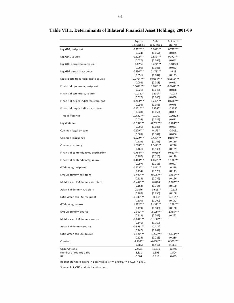
61
Table VII.1. Determinants of Bilateral Financial Asset Holdings, 2001-09
Equity Debt BIS bank
securi ties securi ties cla ims
Log GDP, recipient 0.572*** 0.604*** 0.727***
(0.024) (0.052) (0.035)
Log GDP, source 0.122*** 0.532*** 0.372***
(0.027) (0.065) (0.051)
Log GDP percapita , recipient 0.0764 0.227*** 0.00349
(0.050) (0.081) (0.062)
Log GDP percapita , source 0.430*** 0.478*** -0.18
(0.051) (0.087) (0.123)
Log exports from recipient to source 0.0784*** 0.0364*** 0.0613***
(0.008) (0.013) (0.011)
Financia l openness , recipient 0.0612*** 0.109*** 0.0744***
(0.021) (0.042) (0.028)
Financia l openness , source -0.0320* 0.101** -0.035
(0.017) (0.046) (0.050)
Financia l depth indicator, recipient 0.243*** 0.235*** 0.696***
(0.036) (0.055) (0.075)
Financia l depth indicator, source 0.171*** 0.126** 0.135*
(0.028) (0.053) (0.081)
Time di fference 0.0582*** -0.0307 0.00122
(0.014) (0.023) (0.021)
Log dis tance -0.597*** -0.702*** -0.763***
(0.056) (0.088) (0.081)
Common legal system 0.179*** 0.173* -0.0151
(0.069) (0.101) (0.096)
Common languange 0.622*** 0.420*** 0.879***
(0.119) (0.161) (0.130)
Common currency 1.618*** 1.542*** 0.226
(0.161) (0.136) (0.139)
Financia l center dummy, destination 0.764*** 0.0669 0.621***
(0.107) (0.120) (0.129)
Financia l center dummy, source 0.483*** 1.460*** 1.136***
(0.097) (0.116) (0.097)
G7 dummy, recipient 0.573*** 0.689*** 0.218
(0.134) (0.170) (0.143)
EMEUR dummy, recipient -0.493*** -0.606*** -0.461***
(0.118) (0.235) (0.156)
Middle east EM dummy, recipient -0.444*** 0.0784 -0.967***
(0.153) (0.314) (0.180)
As ian EM dummy, recipient 0.0876 -0.611** -0.115
(0.169) (0.256) (0.158)
Latin American EM, recipient -0.385*** -0.132 0.316**
(0.130) (0.200) (0.142)
G7 dummy, source 1.532*** 1.452*** 1.259***
(0.119) (0.180) (0.130)
EMEUR dummy, source -1.362*** -2.199*** -1.485***
(0.113) (0.247) (0.262)
Middle east EM dummy, source -0.634*** -1.180***
(0.146) (0.360)
As ian EM dummy, source -0.898*** -0.416*
(0.142) (0.244)
Latin American EM, source -0.921*** -1.282*** -2.234***
(0.124) (0.225) (0.230)
Constant -1.798** -4.068*** 6.393***
(0.786) (1.412) (1.383)
Observations 22,631 10,711 10,498
Number of country pa irs 3,511 1,396 1,504
R2 0.664 0.715 0.695
Robust s tandard errors in parentheses : *** p<0.01, ** p<0.05, * p<0.1
Source: BIS, CPIS and s taff estimates .
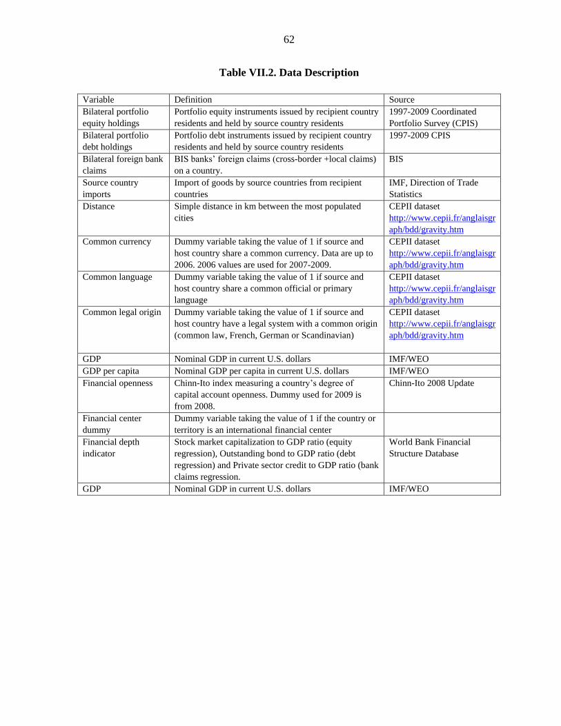
62
Table VII.2. Data Description
Variable Definition Source
Bilateral portfolio
equity holdings
Portfolio equity instruments issued by recipient country
residents and held by source country residents
1997-2009 Coordinated
Portfolio Survey (CPIS)
Bilateral portfolio
debt holdings
Portfolio debt instruments issued by recipient country
residents and held by source country residents
1997-2009 CPIS
Bilateral foreign bank
claims
BIS banks‘ foreign claims (cross-border +local claims)
on a country.
BIS
Source country
imports
Import of goods by source countries from recipient
countries
IMF, Direction of Trade
Statistics
Distance Simple distance in km between the most populated
cities
CEPII dataset
http://www.cepii.fr/anglaisgr
aph/bdd/gravity.htm
Common currency Dummy variable taking the value of 1 if source and
host country share a common currency. Data are up to
2006. 2006 values are used for 2007-2009.
CEPII dataset
http://www.cepii.fr/anglaisgr
aph/bdd/gravity.htm
Common language Dummy variable taking the value of 1 if source and
host country share a common official or primary
language
CEPII dataset
http://www.cepii.fr/anglaisgr
aph/bdd/gravity.htm
Common legal origin Dummy variable taking the value of 1 if source and
host country have a legal system with a common origin
(common law, French, German or Scandinavian)
CEPII dataset
http://www.cepii.fr/anglaisgr
aph/bdd/gravity.htm
GDP Nominal GDP in current U.S. dollars IMF/WEO
GDP per capita Nominal GDP per capita in current U.S. dollars IMF/WEO
Financial openness Chinn-Ito index measuring a country‘s degree of
capital account openness. Dummy used for 2009 is
from 2008.
Chinn-Ito 2008 Update
Financial center
dummy
Dummy variable taking the value of 1 if the country or
territory is an international financial center
Financial depth
indicator
Stock market capitalization to GDP ratio (equity
regression), Outstanding bond to GDP ratio (debt
regression) and Private sector credit to GDP ratio (bank
claims regression.
World Bank Financial
Structure Database
GDP Nominal GDP in current U.S. dollars IMF/WEO
63
References
Allen, F. and D. Gale, 2000, ―Financial Contagion‖, Journal of Political Economy, Vol. 108,
No. 1 pp. 1–33.
Battiston, S., D. Gatti, M. Gallegati, B.C.N. Greenwald, and J.E. Stiglitz, 2009, ―Liasons
Dangereuses: Increasing Connectivity, Risk Sharing, and Systemic Risk,‖ NBER
Working Paper No.15611 (Cambridge, Massachusetts: National Bureau of Economic
Research).
Bayoumi, T., and A. Swiston, 2007, ―The Ties that Bind: Measuring International Bond
Spillovers Using Inflation-Indexed Bond Yields,‖ IMF Working Paper 07/128
(Washington: International Monetary Fund).
———, 2009, ―Foreign Entanglements: Estimating the Source and Size of Spillovers across
Industrial Countries,‖ IMF Staff Papers, International Monetary Fund,Vol. 56, No. 2.
Bordo, M.D. and J.S. Landon, 2010, ―The Global Financial Crisis of 2007-08. Is it
Unprecedented?‖ NBER Working Paper No. 16589 (Cambridge, Massachusetts:
National Bureau of Economic Research).
Borensztein, E. and P. Loungani, 2011, ―Asian Financial Integration: Trends and
Interruptions,‖ IMF Working Paper 11/4 (Washington: International Monetary Fund).
Calvo, G., A. Izquierdo, L.-F. Mejía, 1998, ―Systemic Sudden Stops: The Relevance of
Balance-Sheet Effects and Financial Integration,‖ NBER Working Paper No. 14026 (Cambridge, Massachusetts: National Bureau of Economic Research).
Chuhan, P., S. Claessens, and N. Mamingi, 1993, ―Equity and Bond Flows to Latin America
and Asia: The Role Global and Country Factors,‖ IECIF Policy Research Working
Paper No. 1160 (Washington: World Bank).
Diebold, F.X. and K. Yilmaz, 2009, ―Measuring Financial Asset Return and Volatility
Spillovers, With Application to Global Equity Markets,‖ Economic Journal, Vol. 119,
pp. 158-171
———, 2010, ―Better to Give than to Receive: Predictive Directional Measurement of
Volatility Spillovers,‖ International Journal of Forecasting, forthcoming.
———, 2011, ―Predictive Measurement of Connectedness in Financial and Macroeconomic
Environments,‖ forthcoming.
64
Eichengreen, B. and P. Luengnaruemitchai, 2006. ―Bond Markets as Conduits for Capital
Flows: How Does Asia Compare?‖ NBER Working Paper No. 12408(Cambridge,
Massachusetts: National Bureau of Economic Research).
Fender, I., and P. McGuire, 2010, ―Bank Structure, Funding Risks and the Transmission of
Shocks Across Countries: concepts and measurement,‖ BIS Quarterly Review
September, pp. 63-79
Fernandez-Arias, E., 1996, ―The New Wave of Private Capital Inflows: Push or Pull?‖
Journal of Development Economics, Elsevier, Vol. 48 No.2(March), pp. 389–418.
Fernández-Arias, E. and E. Levy-Yeyati, 2010, ―Global Financial Safety Nets: Where Do We
Go from Here?‖ CIF Working Paper No. 06/2010 (Universidad Torcuato di Tella).
Fernandez-Arias, E. and P. J. Montiel, 1996, ―The Surge in Capital Inflows to Developing
Countries: An Analytical Overview,‖ World Bank Economic Review, Vol. 10 No. 1
(January), pp. 51–77.
Ferrucci, G., V. Herzberg, F. Soussa, and A. Taylor, 2004, ―Understanding Capital Flows to
Emerging Market Economies,‖ Financial Stability Review, London, June.
Galstyan, V., and P. R. Lane, 2010, ―The Dynamics of Portfolio Holdings in Emerging
Europe‖, IIIS Discussion Paper No. 346.
Gai, P. and S. Kapadia, 2010, ―Contagion in Financial Networks,‖ Bank of England Working
Paper No. 383.
Garratt, R., L. Mahadeva, and K. Svirydzenka, 2011, ―Mapping Systemic Risk in the
International Banking Network,‖ Bank of England Working Paper No. 413.
Haldane, A.G., 2009, ―Rethinking the Financial Network‖, Speech delivered at the Financial
Student Association, Amsterdam.
Holmström, B. and J. Tirole, 1998, ―Private and Public Supply of Liquidity,‖ Journal of
Political Economy, Vol., 106, pp. 1–40.
International Monetary Fund, 2007, World Economic Outlook, April 2007: A Survey by the
Staff of the International Monetary Fund, World Economic and Financial Surveys
(Washington).
65
———, 2009a, ―Assessing the Systemic Implications of Financial Linkages‖, in Global
Financial Stability Report: Responding to the Financial Crisis
and Measuring Systemic Risks, World Economic and Financial Surveys, April 2009.
———, 2009b, ―Detecting Systemic Risk‖, in Global Financial Stability Report:
Responding to the Financial Crisis and Measuring Systemic Risks, World Economic
and Financial Surveys, April 2009.
———, 2010a. ―The Fund‘s Role Regarding Cross-Border Capital
Flows‖, IMF Policy Paper (Washington ). Available via the Internet:
www.imf.org/external/np/pp/eng/2010/111510.pdf
———, 2010b, ―Integrating Stability Assessments Under the Financial
Sector Assessment Program into Article IV Surveillance‖, IMF Policy Paper
(Washington ). Available via the Internet:
http://www.imf.org/external/pp/longres.aspx?id=4477
———, 2010c, ―Understanding Financial Interconnectedness‖, IMF
Policy Paper (Washington ). Available via the Internet:
www.imf.org/external/np/pp/eng/2010/100410.pdf
———, 2010d. ―How Did Emerging Markets Cope in the Crisis?‖, IMF
Policy Paper (Washington ). Available via the Internet:
http://www.imf.org/external/pp/longres.aspx?id=4459.
———, 2010e, ―Global Liquidity Expansion: Effects on Receiving
Economies and Policy Response Options‖ in Global Financial Stability Report:
Meeting New Challenges to Stability and Building a Safer System, World Economic
and Financial Surveys, April 2010.
———, 2011a, ―New Growth Drivers for Low–Income Countries - The
Role of BRICs‖, Policy Paper (Washington DC). Available via the Internet:
https://www.imf.org/external/np/pp/eng/2011/011211.pdf
———, 2011b, World Economic Outlook April 2011: A Survey by the Staff of the
International Monetary Fund, World Economic and Financial Surveys (Washington).
———, 2011c, ―Assessing Reserve Adequacy‖, IMF Policy Paper (Washington DC).
Available via the Internet: www.imf.org/external/np/pp/eng/2011/021411b.pdf
———, 2011d, ―Strengthening the International Monetary System: Taking Stock and
Looking Forward‖, IMF Policy Paper (Washington DC). Available via the Internet:
http://www.imf.org/external/pp/longres.aspx?id=4548
66
———, 2011e, ―Recent Experiences in Managing Capital Inflows—
Cross-Cutting Themes and Possible Policy Framework‖, IMF Policy Paper
(Washington DC). Available via the internet:
http://www.imf.org/external/pp/longres.aspx?id=4542
———, 2011f, ―Monitoring Financial Interconnectedness, Including the Data Template for
Global Systemically Important Financial Institutions, IMF Policy Paper,‖ upcoming
IMF Policy Paper (Washington DC).
Kubelec, K and F. Sa, 2010, ―The Geographical Composition of National External Balance
Sheets: 1980-2005‖, Bank of England Working Paper No. 384
Lane, P. R., 2009, ―The Global Crisis and Capital Flows to Emerging Markets,‖ in
Macroeconomic Stability and Financial Regulation: Key Issues for the G20 (edited by
Mathias Dewatripoint, Xavier Freixas and Richard Portes), VOX e-book.
Lane, P. R. and G. M. Milesi-Ferretti, 2007, ―The External Wealth of Nations Mark II:
Revised and Extended Estimates of Foreign Assets and Liabilities, 1970-2004,‖
Journal of International Economics, Vol. 73 (November) pp. 223–250.
———, 2008, ―International Investment Patterns‖, The Review of Economics and Statistics,
Vol. 90 No.3, pp. 538–49.
Magud, N., C. M. Reinhart, and K. S. Rogoff, 2011, ―Capital Controls: Myth and Reality – A
Portfolio Balance Approach,‖ NBER Working Paper No. 16805 (Cambridge,
Massachusetts: National Bureau of Economic Research).
Mody, A., M. P. Taylor, and J. Y. Kim, J.Y. 2001, ―Modeling Fundamentals for Forecasting
Capital Flows to Emerging Markets,‖ International Journal of Finance and
Economics, Vol. 6, pp.201–206.
Milesi-Ferretti, G. M., F. Strobbe, and N. Tamirisa, 2010, ―Bilateral Financial Linkages and
Global Imbalances: A View on the Eve of the Financial Crisis‖, IMF Working Paper
10/257 (Washington: International Monetary Fund).
Porter, N. and C. Serra, 2011, ―Cross-border Spillovers Within Banking Groups‖,
forthcoming IMF Working Paper (unpublished; Washington: International Monetary
Fund).
Portes, R., and H. Rey, ―The Determinants of Cross-Border Equity Flows,‖ Journal of
International Economics, Vol. 65 No. 2 (2005), pp. 269–296.
Rose, A. K., and M. Spiegel, 2004, ―A Gravity Model of Sovereign Lending: Trade, Default
and Credit,‖ Staff Papers, International Monetary Fund, Vol 51:S, 64–74.
67
Stock, J. H. and M. W. Watson, 2003, ―Understanding Changes in International Business
Cycle Dynamics,‖ NBER Working Paper No. 9859 (Cambridge, Massachusetts:
National Bureau of Economic Research).
von Peter, G., 2007, ―International Banking Centres: A Network Perspective,‖ BIS Quarterly
Review, December, pp. 33-45.