Maple for Math Majors

Roger KraftDepartment of Mathematics, Computer Science, and Statistics

Purdue University Calumetroger@purduecal.edu

4. Functions in Maple

4.1. IntroductionFunctions play a major role in Mathematics so it is important to know how to work with them in Maple. There are two distinct ways to represent a mathematical function in Maple. We can represent a mathematical function using either an "expression" or a "Maple function". The distinction that Maple makes between "expressions" and "functions" has its roots in concepts from both Mathematics and Computer Science. Making this distinction, and learning to understand it and work with it, will help us to better understand how we use ideas like function, equation, and variables in Mathematics, and it will also help introduce us to the Computer Science ideas of a "data structure" and a "procedure".

>

4.2. Functions in Mathematics

4.2.1 ReviewWe quickly review here the definition of a mathematical function. A function is three things bundled together. It is a set of input values (the domain), a set of output values (the codomain), and a rule for associating one of the output values to each of the input values. Functions can be defined in several ways, for example by formulas, by tables, and by graphs. Most of the time in mathematics, the sets of input and output values are sets of numbers. For most people, the "rule" part of a function's definition is the only part that they consider, but that is not a good way to think about functions. To demonstrate that a mathematical function is really more than just its rule, let us look at an example.

>

We shall define three different functions named f, g, and h. The rule for each of these functions will be given by a formula. In fact we will use the same formula in all three cases. What will make the three functions different will be their domains.

The function f has as its domain the set of all real numbers, its codomain is the set of all

positive real numbers, and its rule is given by the formula = ( )f x x2.

The function g has as its domain the set of all positive real numbers, its codomain is the set of

all positive real numbers, and its rule is given by the formula = ( )g x x2.

The function h has as its domain the set of all negative real numbers, its codomain is the set of

all positive real numbers, and its rule is given by the formula = ( )h x x2.

Exercise: Draw graphs for each of the functions f, g, and h.>

How do we know that these three functions are different? The answer is that they have different properties. For example, in the last exercise you should have seen that the functions have three different graphs. As another example, the function f is not invertible (why?), but the functions g and h are both invertible (why?) but they have different inverses. The inverse of the function g

has its rule given by the formula = ( )( )g( )−1

x x . The inverse of the function h has its rule

given by the formula = ( )( )h( )−1

x − x .

So f, g, and h all have the exact same formula (i.e., rule) but they are not the same function. The domain (and codomain) really are important parts of the definition of a mathematical function.

Exercise: What are the domain and codomain for each of g( )−1

and h( )−1

?>

>

4.2.2 Classifying FunctionsYou have used functions extensively in Calculus, Linear Algebra, and Differential Equations classes. In all of those classes, the domain and codomain are always sets of numbers and these sets of numbers are almost always subsets of either the real line, the plane, or 3-dimensional space. We can use this observation to create a useful classification for the kinds of functions that you see most often in those mathematics classes.

Our classification of functions will be based on the dimensions of a function's domain and

codomain. For example, consider a function like = ( )f x − x3 2 + x 10. The domain of this function is a subset of the real line and this function's codomain is also a subset of the real line. In other words, we plug one number into this function and we get out from the function another number. We will call this a "real valued function of a real variable".

Now consider the function = ( )f ,x y + x2 y2. The domain of this function is the plane and its codomain is a subset of the real line. We plug two numbers into this function and we get out from the function a single number. We will call this a "real valued function of two real variables."

For a third example, conside the function = ( )f t ( ),t2 + t ( )cos t . The domain of this function is the real line, and the codomain is a subset of the plane. We plug one number into this function and we get out two numbers in an ordered pair (that is, a point in the plane). We will call this a "2-dimensional vector valued function of a real variable". The phrase "vector valued" is common in mathematics and you can think of it as a synonym for "point valued". We have a function where we plug in a number but we get out a point in the plane (and a point in the plane can also be considered as a vector in the plane).

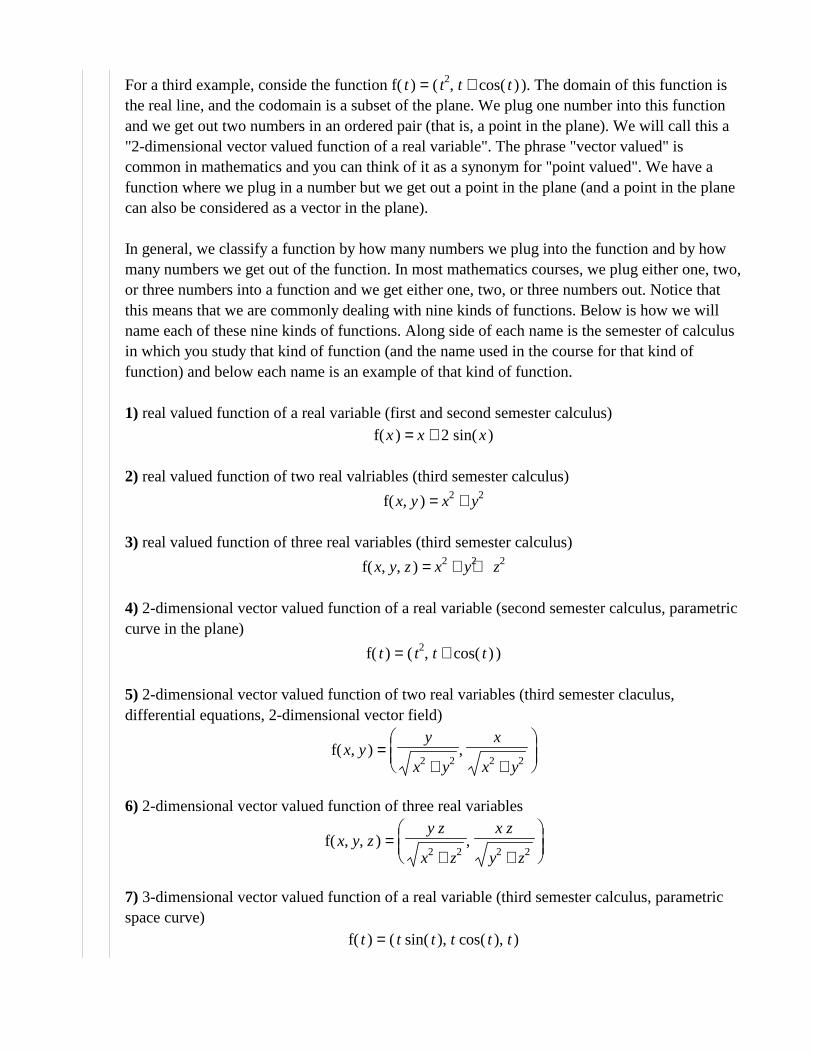
In general, we classify a function by how many numbers we plug into the function and by how many numbers we get out of the function. In most mathematics courses, we plug either one, two, or three numbers into a function and we get either one, two, or three numbers out. Notice that this means that we are commonly dealing with nine kinds of functions. Below is how we will name each of these nine kinds of functions. Along side of each name is the semester of calculus in which you study that kind of function (and the name used in the course for that kind of function) and below each name is an example of that kind of function.

1) real valued function of a real variable (first and second semester calculus) = ( )f x + x 2 ( )sin x

2) real valued function of two real valriables (third semester calculus)

= ( )f ,x y + x2 y2

3) real valued function of three real variables (third semester calculus)

= ( )f , ,x y z + + x2 y2 z2

4) 2-dimensional vector valued function of a real variable (second semester calculus, parametric curve in the plane)

= ( )f t ( ),t2 + t ( )cos t

5) 2-dimensional vector valued function of two real variables (third semester claculus, differential equations, 2-dimensional vector field)

= ( )f ,x y�

����

�

����,

y

+ x2 y2

x

+ x2 y2

6) 2-dimensional vector valued function of three real variables

= ( )f , ,x y z�

����

�

����,

y z

+ x2 z2

x z

+ y2 z2

7) 3-dimensional vector valued function of a real variable (third semester calculus, parametric space curve)

= ( )f t ( ), ,t ( )sin t t ( )cos t t

8) 3-dimensional vector valued function of two real variables (third semester calculus, parametric surface)

= ( )f ,u v ( ), ,( ) + 2 ( )sin v ( )cos u ( ) + 2 ( )sin v ( )sin u + u ( )cos v

9) 3-dimensional vector valued function of three real variables (differential equations, 3-dimensional vector field)

= ( )f , ,x y z ( ), ,2 x 2 y 1

It is important to realize that these nine kinds of functions are not the only kinds of function. They are just the most common kinds that you see in calculus classes. For example, here is a four dimensional vector valued function of five real variables.

= ( )f , , , ,u v t α β ( ), , ,uα vβ + + α β t tIn mathematics we can define functions with any number of inputs and any number of outputs (even including functions with an infinite number of inputs and an infinite number of outputs, which are the subject of a branch of mathematics called Functional Analysis).

>

4.3. Functions in MapleWe mentioned earlier that there are two ways to represent mathematical functions in Maple, as Maple expressions and as Maple functions. In this section we introduce these two representations and in the next section we look at examples that show how to work with them. These two ways of representing mathematical functions are not equivalent. Each way has its advantages and disadvantages. The differences between these two representations can be subtle and non-obvious. To fully understand these differences we will eventually need to learn about several topics from Maple programming. In particular, a full explanation of the differences between expressions and Maple functions requires an understanding of evaluation rules, data structures, procedures, local, global, and lexical variables, parameter passing, remember tables, and a few other ideas. We will cover all of these ideas in the worksheets about Maple programming.

Let us first look at mathematical functions represented as Maple expressions. We define an expression in Maple as just about any mathematical formula that you can write down that does not have an equal sign or any inequalities in it. Here are some examples of expressions.

> 3*x^2 - 5*x + 17;> sin( (x+1)^b ) + ln(y);> exp(x+y)/sec(x);> n! + sum(n^2, n);> a*x + b*y + c*z;

Notice that some of these are expressions in one variable, others are expressions in two or more variables. (How many variables are in the last expression?) Also notice that calls to Maple procedures are allowed as parts of an expression.

>

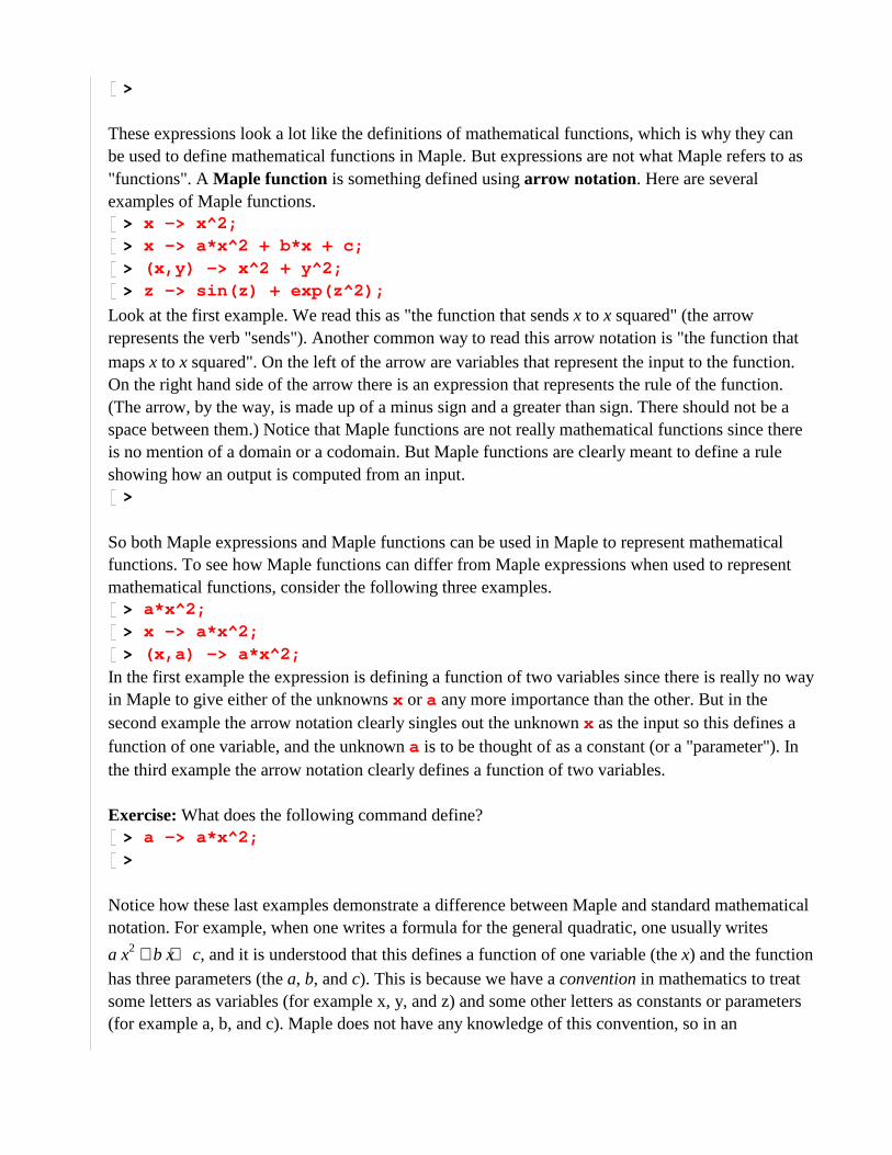
These expressions look a lot like the definitions of mathematical functions, which is why they can be used to define mathematical functions in Maple. But expressions are not what Maple refers to as "functions". A Maple function is something defined using arrow notation. Here are several examples of Maple functions.

> x -> x^2;> x -> a*x^2 + b*x + c;> (x,y) -> x^2 + y^2;> z -> sin(z) + exp(z^2);

Look at the first example. We read this as "the function that sends x to x squared" (the arrow represents the verb "sends"). Another common way to read this arrow notation is "the function that maps x to x squared". On the left of the arrow are variables that represent the input to the function. On the right hand side of the arrow there is an expression that represents the rule of the function. (The arrow, by the way, is made up of a minus sign and a greater than sign. There should not be a space between them.) Notice that Maple functions are not really mathematical functions since there is no mention of a domain or a codomain. But Maple functions are clearly meant to define a rule showing how an output is computed from an input.

>

So both Maple expressions and Maple functions can be used in Maple to represent mathematical functions. To see how Maple functions can differ from Maple expressions when used to represent mathematical functions, consider the following three examples.

> a*x^2;> x -> a*x^2;> (x,a) -> a*x^2;

In the first example the expression is defining a function of two variables since there is really no way in Maple to give either of the unknowns x or a any more importance than the other. But in the second example the arrow notation clearly singles out the unknown x as the input so this defines a function of one variable, and the unknown a is to be thought of as a constant (or a "parameter"). In the third example the arrow notation clearly defines a function of two variables.

Exercise: What does the following command define?> a -> a*x^2;>

Notice how these last examples demonstrate a difference between Maple and standard mathematical notation. For example, when one writes a formula for the general quadratic, one usually writes

+ + a x2 b x c, and it is understood that this defines a function of one variable (the x) and the function has three parameters (the a, b, and c). This is because we have a convention in mathematics to treat some letters as variables (for example x, y, and z) and some other letters as constants or parameters (for example a, b, and c). Maple does not have any knowledge of this convention, so in an

expression Maple treats all unassigned names (i.e., all unknowns) as variables.

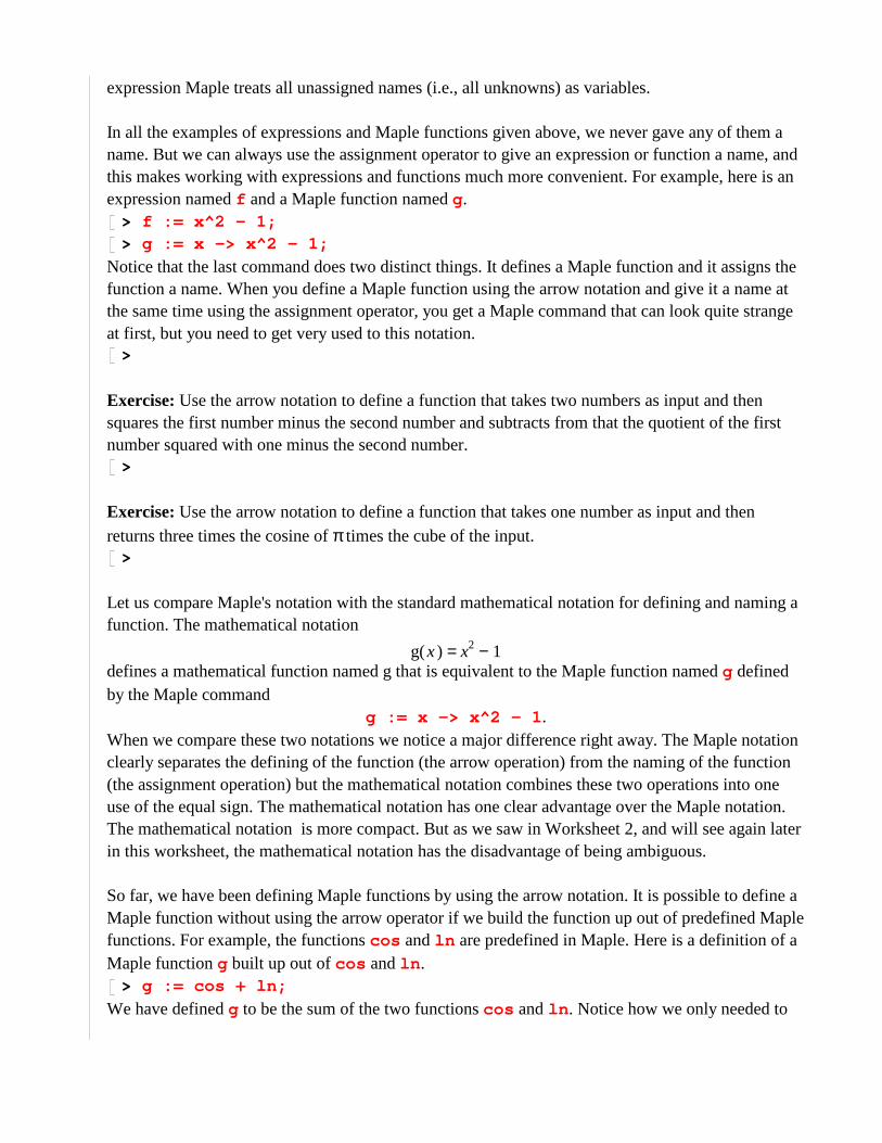
In all the examples of expressions and Maple functions given above, we never gave any of them a name. But we can always use the assignment operator to give an expression or function a name, and this makes working with expressions and functions much more convenient. For example, here is an expression named f and a Maple function named g.

> f := x^2 - 1;> g := x -> x^2 - 1;

Notice that the last command does two distinct things. It defines a Maple function and it assigns the function a name. When you define a Maple function using the arrow notation and give it a name at the same time using the assignment operator, you get a Maple command that can look quite strange at first, but you need to get very used to this notation.

>

Exercise: Use the arrow notation to define a function that takes two numbers as input and then squares the first number minus the second number and subtracts from that the quotient of the first number squared with one minus the second number.

>

Exercise: Use the arrow notation to define a function that takes one number as input and then returns three times the cosine of π times the cube of the input.

>

Let us compare Maple's notation with the standard mathematical notation for defining and naming a function. The mathematical notation

= ( )g x − x2 1defines a mathematical function named g that is equivalent to the Maple function named g defined by the Maple command

g := x -> x^2 - 1 .When we compare these two notations we notice a major difference right away. The Maple notation clearly separates the defining of the function (the arrow operation) from the naming of the function (the assignment operation) but the mathematical notation combines these two operations into one use of the equal sign. The mathematical notation has one clear advantage over the Maple notation. The mathematical notation is more compact. But as we saw in Worksheet 2, and will see again later in this worksheet, the mathematical notation has the disadvantage of being ambiguous.

So far, we have been defining Maple functions by using the arrow notation. It is possible to define a Maple function without using the arrow operator if we build the function up out of predefined Maple functions. For example, the functions cos and ln are predefined in Maple. Here is a definition of a Maple function g built up out of cos and ln .

> g := cos + ln;

We have defined g to be the sum of the two functions cos and ln . Notice how we only needed to

tell Maple the names of the functions involved. We did not need to use any variables in the definition of g. Since g is a Maple function, we can evaluate g at an input using regular function notation.

> g(Pi);> g(a);

Here is a more subtle example.> h := cos + (x -> 3*x-1);

We have defined h as the sum of two predefined functions, the predefined function named cos and the function x->3*x-1 . The later function can be considered as "predefined" in this example because Maple must evaluate the definition x->3*x-1 before it can evaluate the addition that defines h.

> h(z);>

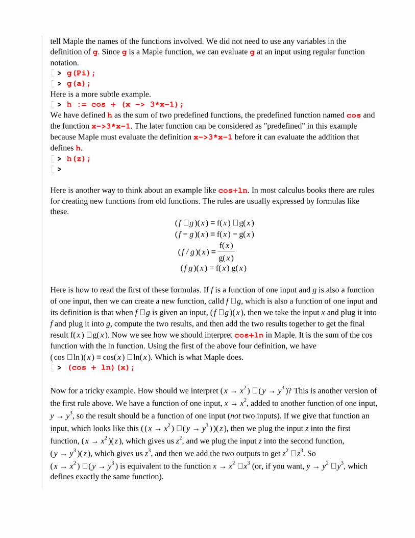
Here is another way to think about an example like cos+ln . In most calculus books there are rules for creating new functions from old functions. The rules are usually expressed by formulas like these.

= ( )( ) + f g x + ( )f x ( )g x

= ( )( ) − f g x − ( )f x ( )g x

= ( )( )f / g x( )f x

( )g x

= ( )( )f g x ( )f x ( )g x

Here is how to read the first of these formulas. If f is a function of one input and g is also a function of one input, then we can create a new function, calld + f g, which is also a function of one input and its definition is that when + f g is given an input, ( )( ) + f g x , then we take the input x and plug it into f and plug it into g, compute the two results, and then add the two results together to get the final result + ( )f x ( )g x . Now we see how we should interpret cos+ln in Maple. It is the sum of the cos function with the ln function. Using the first of the above four definition, we have

= ( )( ) + cos ln x + ( )cos x ( )ln x . Which is what Maple does.> (cos + ln)(x);

Now for a tricky example. How should we interpret + ( ) → x x2 ( ) → y y3 ? This is another version of

the first rule above. We have a function of one input, → x x2, added to another function of one input,

→ y y3, so the result should be a function of one input (not two inputs). If we give that function an

input, which looks like this ( )( ) + ( ) → x x2 ( ) → y y3 z , then we plug the input z into the first

function, ( )( ) → x x2 z , which gives us z2, and we plug the input z into the second function,

( )( ) → y y3 z , which gives us z3, and then we add the two outputs to get + z2 z3. So

+ ( ) → x x2 ( ) → y y3 is equivalent to the function → x + x2 x3 (or, if you want, → y + y2 y3, which defines exactly the same function).

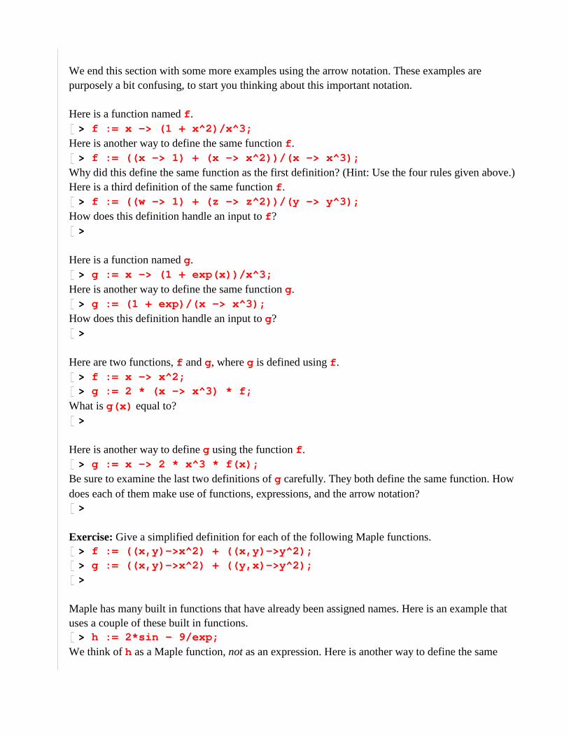
We end this section with some more examples using the arrow notation. These examples are purposely a bit confusing, to start you thinking about this important notation.

Here is a function named f .> f := x -> (1 + x^2)/x^3;

Here is another way to define the same function f .> f := ((x -> 1) + (x -> x^2))/(x -> x^3);

Why did this define the same function as the first definition? (Hint: Use the four rules given above.) Here is a third definition of the same function f .

> f := ((w -> 1) + (z -> z^2))/(y -> y^3);

How does this definition handle an input to f ?>

Here is a function named g.> g := x -> (1 + exp(x))/x^3;

Here is another way to define the same function g.> g := (1 + exp)/(x -> x^3);

How does this definition handle an input to g?>

Here are two functions, f and g, where g is defined using f .> f := x -> x^2;> g := 2 * (x -> x^3) * f;

What is g(x) equal to?>

Here is another way to define g using the function f .> g := x -> 2 * x^3 * f(x);

Be sure to examine the last two definitions of g carefully. They both define the same function. How does each of them make use of functions, expressions, and the arrow notation?

>

Exercise: Give a simplified definition for each of the following Maple functions.> f := ((x,y)->x^2) + ((x,y)->y^2);> g := ((x,y)->x^2) + ((y,x)->y^2);>

Maple has many built in functions that have already been assigned names. Here is an example that uses a couple of these built in functions.

> h := 2*sin - 9/exp;

We think of h as a Maple function, not as an expression. Here is another way to define the same

function h.> h := x -> 2*sin(x) - 9/exp(x);>

Exercise: The 2 in the following definition of h does not have the same meaning as the 2 in the following definition of f . Explain the different meanings of these two 2's.

> h := 2 + exp;> f := x -> 2 + exp(x);>

>

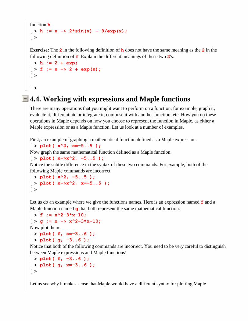
4.4. Working with expressions and Maple functionsThere are many operations that you might want to perform on a function, for example, graph it, evaluate it, differentiate or integrate it, compose it with another function, etc. How you do these operations in Maple depends on how you choose to represent the function in Maple, as either a Maple expression or as a Maple function. Let us look at a number of examples.

First, an example of graphing a mathematical function defined as a Maple expression.> plot( x^2, x=-5..5 );

Now graph the same mathematical function defined as a Maple function. > plot( x->x^2, -5..5 );

Notice the subtle difference in the syntax of these two commands. For example, both of the following Maple commands are incorrect.

> plot( x^2, -5..5 );> plot( x->x^2, x=-5..5 );>

Let us do an example where we give the functions names. Here is an expression named f and a Maple function named g that both represent the same mathematical function.

> f := x^2-3*x-10;> g := x -> x^2-3*x-10;

Now plot them.> plot( f, x=-3..6 );> plot( g, -3..6 );

Notice that both of the following commands are incorrect. You need to be very careful to distinguish between Maple expressions and Maple functions!

> plot( f, -3..6 );> plot( g, x=-3..6 );>

Let us see why it makes sense that Maple would have a different syntax for plotting Maple

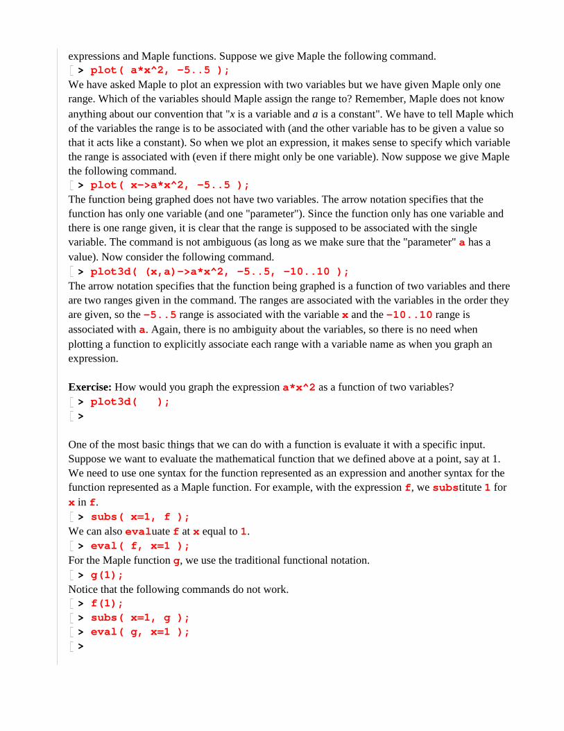
expressions and Maple functions. Suppose we give Maple the following command.> plot( a*x^2, -5..5 );

We have asked Maple to plot an expression with two variables but we have given Maple only one range. Which of the variables should Maple assign the range to? Remember, Maple does not know anything about our convention that "x is a variable and a is a constant". We have to tell Maple which of the variables the range is to be associated with (and the other variable has to be given a value so that it acts like a constant). So when we plot an expression, it makes sense to specify which variable the range is associated with (even if there might only be one variable). Now suppose we give Maple the following command.

> plot( x->a*x^2, -5..5 );

The function being graphed does not have two variables. The arrow notation specifies that the function has only one variable (and one "parameter"). Since the function only has one variable and there is one range given, it is clear that the range is supposed to be associated with the single variable. The command is not ambiguous (as long as we make sure that the "parameter" a has a value). Now consider the following command.

> plot3d( (x,a)->a*x^2, -5..5, -10..10 );

The arrow notation specifies that the function being graphed is a function of two variables and there are two ranges given in the command. The ranges are associated with the variables in the order they are given, so the -5..5 range is associated with the variable x and the -10..10 range is associated with a. Again, there is no ambiguity about the variables, so there is no need when plotting a function to explicitly associate each range with a variable name as when you graph an expression.

Exercise: How would you graph the expression a*x^2 as a function of two variables?> plot3d( );>

One of the most basic things that we can do with a function is evaluate it with a specific input. Suppose we want to evaluate the mathematical function that we defined above at a point, say at 1. We need to use one syntax for the function represented as an expression and another syntax for the function represented as a Maple function. For example, with the expression f , we subs titute 1 for x in f .

> subs( x=1, f );

We can also eval uate f at x equal to 1.> eval( f, x=1 );

For the Maple function g, we use the traditional functional notation.> g(1);

Notice that the following commands do not work.> f(1);> subs( x=1, g );> eval( g, x=1 );>

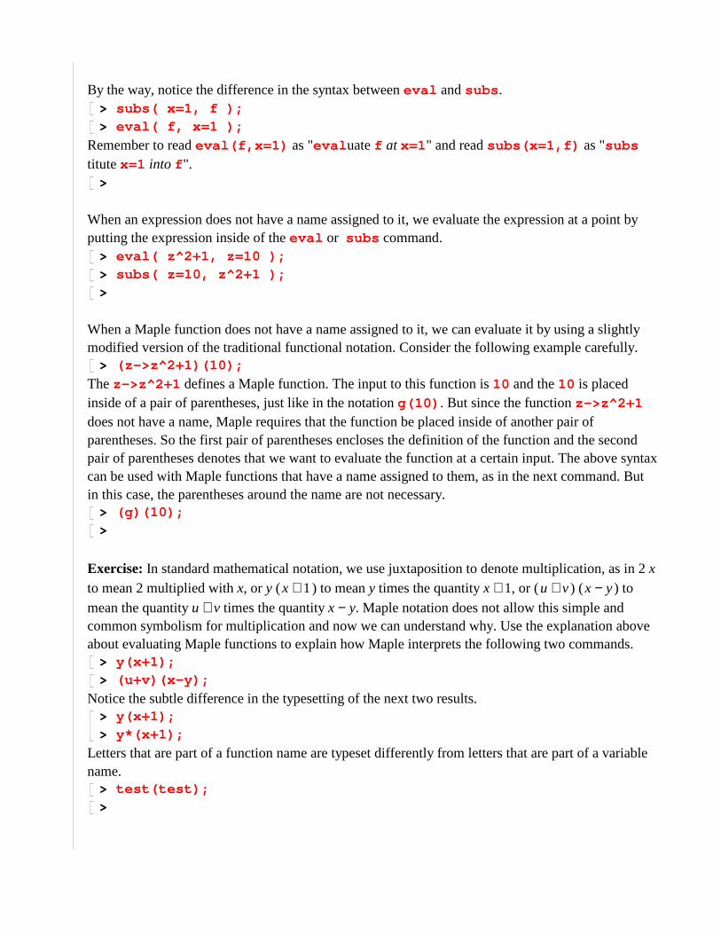
By the way, notice the difference in the syntax between eval and subs .> subs( x=1, f );> eval( f, x=1 );

Remember to read eval(f,x=1) as "eval uate f at x=1 " and read subs(x=1,f) as "subs

titute x=1 into f ".>

When an expression does not have a name assigned to it, we evaluate the expression at a point by putting the expression inside of the eval or subs command.

> eval( z^2+1, z=10 );> subs( z=10, z^2+1 );>

When a Maple function does not have a name assigned to it, we can evaluate it by using a slightly modified version of the traditional functional notation. Consider the following example carefully.

> (z->z^2+1)(10);

The z->z^2+1 defines a Maple function. The input to this function is 10 and the 10 is placed inside of a pair of parentheses, just like in the notation g(10) . But since the function z->z^2+1 does not have a name, Maple requires that the function be placed inside of another pair of parentheses. So the first pair of parentheses encloses the definition of the function and the second pair of parentheses denotes that we want to evaluate the function at a certain input. The above syntax can be used with Maple functions that have a name assigned to them, as in the next command. But in this case, the parentheses around the name are not necessary.

> (g)(10);>

Exercise: In standard mathematical notation, we use juxtaposition to denote multiplication, as in 2 x to mean 2 multiplied with x, or y ( ) + x 1 to mean y times the quantity + x 1, or ( ) + u v ( ) − x y to mean the quantity + u v times the quantity − x y. Maple notation does not allow this simple and common symbolism for multiplication and now we can understand why. Use the explanation above about evaluating Maple functions to explain how Maple interprets the following two commands.

> y(x+1);> (u+v)(x-y);

Notice the subtle difference in the typesetting of the next two results.> y(x+1);> y*(x+1);

Letters that are part of a function name are typeset differently from letters that are part of a variable name.

> test(test);>

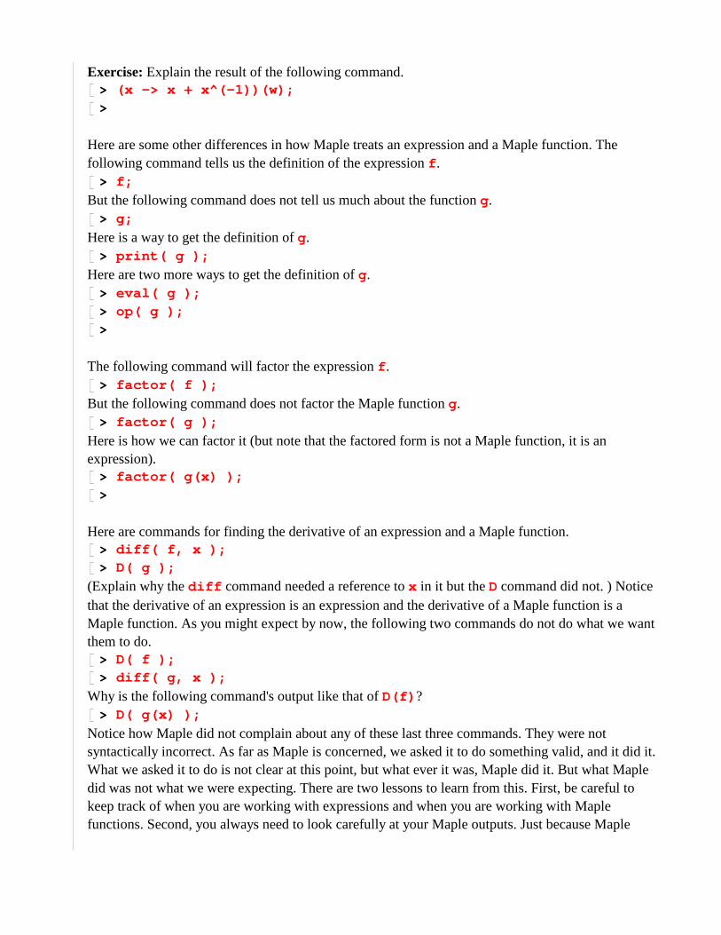
Exercise: Explain the result of the following command.> (x -> x + x^(-1))(w);>

Here are some other differences in how Maple treats an expression and a Maple function. The following command tells us the definition of the expression f .

> f;

But the following command does not tell us much about the function g.> g;

Here is a way to get the definition of g.> print( g );

Here are two more ways to get the definition of g.> eval( g );> op( g );>

The following command will factor the expression f .> factor( f );

But the following command does not factor the Maple function g.> factor( g );

Here is how we can factor it (but note that the factored form is not a Maple function, it is an expression).

> factor( g(x) );>

Here are commands for finding the derivative of an expression and a Maple function.> diff( f, x );> D( g );

(Explain why the diff command needed a reference to x in it but the D command did not. ) Notice that the derivative of an expression is an expression and the derivative of a Maple function is a Maple function. As you might expect by now, the following two commands do not do what we want them to do.

> D( f );> diff( g, x );

Why is the following command's output like that of D(f) ?> D( g(x) );

Notice how Maple did not complain about any of these last three commands. They were not syntactically incorrect. As far as Maple is concerned, we asked it to do something valid, and it did it. What we asked it to do is not clear at this point, but what ever it was, Maple did it. But what Maple did was not what we were expecting. There are two lessons to learn from this. First, be careful to keep track of when you are working with expressions and when you are working with Maple functions. Second, you always need to look carefully at your Maple outputs. Just because Maple

computes something does not mean that it computed something that makes sense or that it computed what you wanted it to compute.

>

Let us do an example of combining two mathematical functions f and g by composing them to make a new function h(x) = f(g(x). Here is how we would compose two mathematical functions if they are represented by expressions.

> f := x^2 + 3*x;> g := x + 1;> h := subs( x=g, f );

We substituted the inner function g into the outer function f and got the expression h that represents the composition f(g(x)). We can also do this using eval .

> h := eval( f, x=g );

Here is how we would do this if f and g are represented by Maple functions.> f := x -> x^2 + 3*x;> g := x -> x + 1;> h := f@g;

Here is how we can verify that the Maple function h represents the composition of f and g.> h(x);

We do not need to use a separate name like h for the composition of the Maple functions f and g. The symbol f@g can be used as a name for the composition, but we need to put parentheses around this name when we use it to evaluate the composition.

> (f@g)(x);

The at sign (@) is used in Maple to mean composition of two Maple functions. The at sign is used because it is the closest character on the standard computer keyboard to the little raised circle used in mathematics books to denote composition of functions. (If you do not remember the symbol, look up composition in almost any calculus book.)

If f and g are Maple functions, we can also compose them by using the following notation.> f(g);

Since f(g) is a Maple function, we can apply it to an input variable in order to see what the definition of f(g) is.

> f(g)(x);

When f and g are Maple functions, there is even a third way to express their composition.> f(g(x));

Notice that f(g(x)) is different from f@g and f(g) in that the latter two are Maple functions, but f(g(x)) is an expression. Also notice the subtle difference between f(g(x)) and f(g)(x) . In f(g(x)) , we take the expression g(x) and plug it into the Maple function f and get the expression f(g(x)) . In f(g)(x) , we take the Maple function g and compose it with the Maple function f , and then we evaluate the resulting Maple function at the input x which results in the expression f(g)(x) .

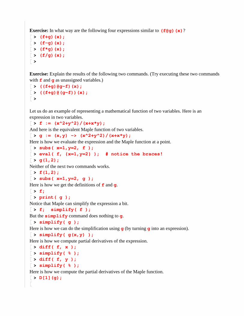
Exercise: In what way are the following four expressions similar to (f@g)(x) ?> (f+g)(x);> (f-g)(x);> (f*g)(x);> (f/g)(x);>

Exercise: Explain the results of the following two commands. (Try executing these two commands with f and g as unassigned variables.)

> ((f+g)@g-f)(x);> ((f+g)@(g-f))(x);>

Let us do an example of representing a mathematical function of two variables. Here is an expression in two variables.

> f := (x^2+y^2)/(x+x*y);

And here is the equivalent Maple function of two variables.> g := (x,y) -> (x^2+y^2)/(x+x*y);

Here is how we evaluate the expression and the Maple function at a point.> subs( x=1,y=2, f );> eval( f, {x=1,y=2} ); # notice the braces!> g(1,2);

Neither of the next two commands works.> f(1,2);> subs( x=1,y=2, g );

Here is how we get the definitions of f and g.> f;> print( g );

Notice that Maple can simplify the expression a bit.> f; simplify( f );

But the simplify command does nothing to g.> simplify( g );

Here is how we can do the simplification using g (by turning g into an expression).> simplify( g(x,y) );

Here is how we compute partial derivatives of the expression.> diff( f, x );> simplify( % );> diff( f, y );> simplify( % );

Here is how we compute the partial derivatives of the Maple function.> D[1](g);

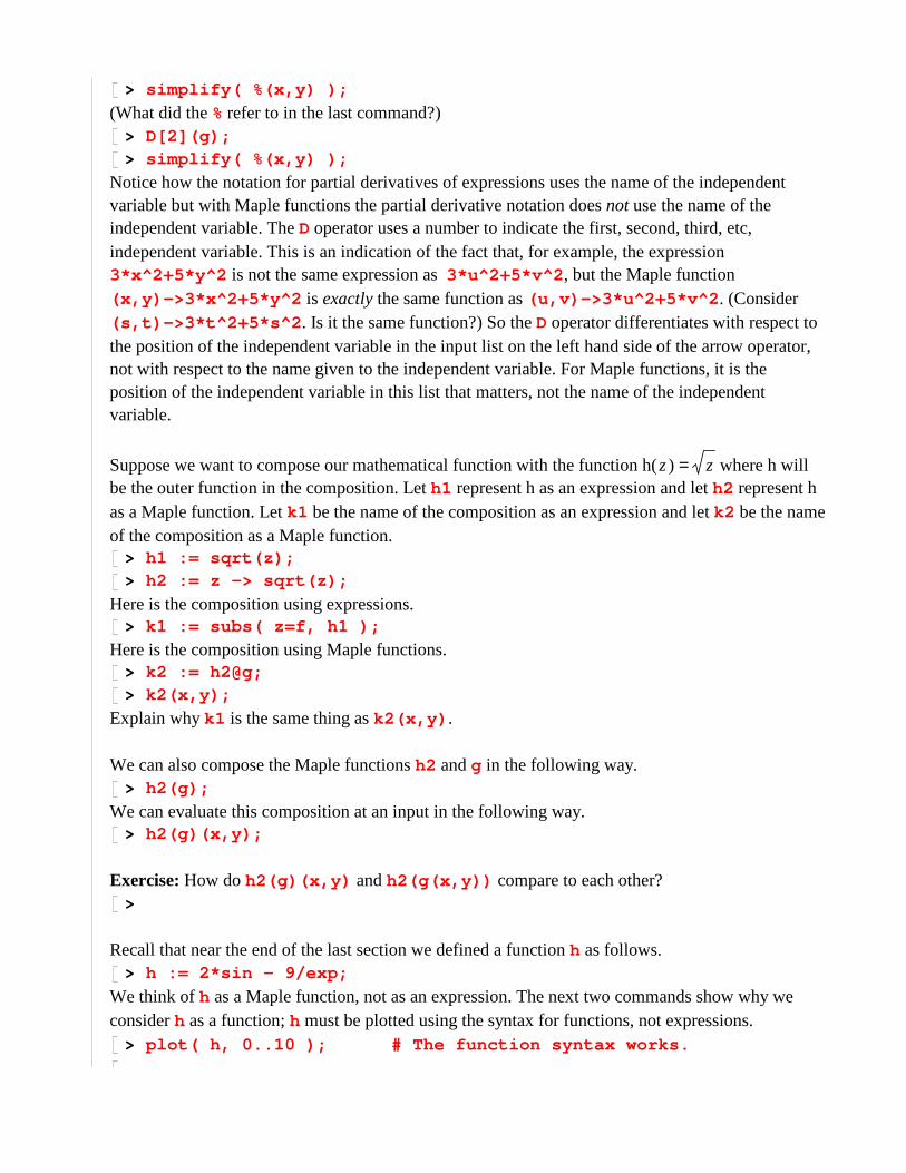
> simplify( %(x,y) );

(What did the % refer to in the last command?)> D[2](g);> simplify( %(x,y) );

Notice how the notation for partial derivatives of expressions uses the name of the independent variable but with Maple functions the partial derivative notation does not use the name of the independent variable. The D operator uses a number to indicate the first, second, third, etc, independent variable. This is an indication of the fact that, for example, the expression 3*x^2+5*y^2 is not the same expression as 3*u^2+5*v^2 , but the Maple function (x,y)->3*x^2+5*y^2 is exactly the same function as (u,v)->3*u^2+5*v^2 . (Consider (s,t)->3*t^2+5*s^2 . Is it the same function?) So the D operator differentiates with respect to the position of the independent variable in the input list on the left hand side of the arrow operator, not with respect to the name given to the independent variable. For Maple functions, it is the position of the independent variable in this list that matters, not the name of the independent variable.

Suppose we want to compose our mathematical function with the function = ( )h z z where h will be the outer function in the composition. Let h1 represent h as an expression and let h2 represent h as a Maple function. Let k1 be the name of the composition as an expression and let k2 be the name of the composition as a Maple function.

> h1 := sqrt(z);> h2 := z -> sqrt(z);

Here is the composition using expressions.> k1 := subs( z=f, h1 );

Here is the composition using Maple functions.> k2 := h2@g;> k2(x,y);

Explain why k1 is the same thing as k2(x,y) .

We can also compose the Maple functions h2 and g in the following way.> h2(g);

We can evaluate this composition at an input in the following way.> h2(g)(x,y);

Exercise: How do h2(g)(x,y) and h2(g(x,y)) compare to each other?>

Recall that near the end of the last section we defined a function h as follows.> h := 2*sin - 9/exp;

We think of h as a Maple function, not as an expression. The next two commands show why we consider h as a function; h must be plotted using the syntax for functions, not expressions.

> plot( h, 0..10 ); # The function syntax works.

> plot( h, x = 0..10 ); # The expression syntax does not work.

Here is another way to define the same function h.> h := x -> 2*sin(x) - 9/exp(x);>

Exercise: Explain in detail the steps that Maple uses to automatically simplify the following command.

> f := ((x,y)->((x,y)->x*y)(x,x)+((u,v)->u+v)(3,y))(s,t);>

Exercise: Change a single character in the following command so that the Maple function defined is equivalent to the zero function.

> (x,y)->(((x,y)->x^2+y)(x,x)-((x,y)->x+x)(x^2,x));>

Exercise: Let = ( )f ,x y + 3 x 5 y and let = ( )h z + z 1. We have already seen how to compute the composition h(f( ,x y)) using either expressions or Maple functions. Explain why the composition f(h(z)) does not make sense mathematically. Compute the compositions f(h(x),y), f(x,h(y)), and f(h(x),h(y)). First do this exercise using expressions. Can you do these compositions using Maple functions and the @ operator?

>

Exercise: Let f be the following function of two variables.> f := (x,y) -> 3*x^2+5*y^2;

If we hold one of the inputs to f fixed, then we get a function of one variable that we will call a "slice of f ". Let fx3 be the slice of f defined by letting y be fixed at 3. Find a Maple command that uses f to define fx3 as a Maple function.

>

Let f3y denote the slice of f with x fixed at 3. Use f to define f3y as a Maple function.>

Explain the mathematical meaning of diff(fx3(x),x) and diff(f3y(y),y) . (The following two commands do not mean anything until you have properly defined fx3 and f3y .)

> diff( fx3(x), x );> diff( f3y(y), y );

Find another way to compute diff(fx3(x),x) and diff(f3y(y),y) that does not use the slice functions fx3 and fy3 .Note: The following Maple command represents fx3 as an expression, so it is not the correct answer to the first part of this exercise.

> fx3 := f(x,3);>

Almost anything we would like to do with an expression we can do with a Maple function, and visa

versa. Unfortunately, as we have seen above, the syntax for doing the same thing with an expression and a Maple function can be quite different. Is one of the two methods "better" than the other? Most people do most of their Maple work using expressions to represent mathematical functions. Overall, expressions seem to be a bit easier to work with. But Maple functions are indispensable at times, so you must get used to working with both concepts.

>

>

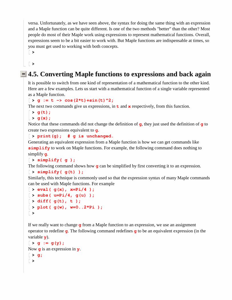
4.5. Converting Maple functions to expressions and back againIt is possible to switch from one kind of representation of a mathematical function to the other kind. Here are a few examples. Lets us start with a mathematical function of a single variable represented as a Maple function.

> g := t -> cos(2*t)+sin(t)^2;

The next two commands give us expressions, in t and x respectively, from this function.> g(t);> g(x);

Notice that these commands did not change the definition of g, they just used the definition of g to create two expressions equivalent to g.

> print(g); # g is unchanged.

Generating an equivalent expression from a Maple function is how we can get commands like simplify to work on Maple functions. For example, the following command does nothing to simplify g.

> simplify( g );

The following command shows how g can be simplified by first converting it to an expression.> simplify( g(t) );

Similarly, this technique is commonly used so that the expression syntax of many Maple commands can be used with Maple functions. For example

> eval( g(x), x=Pi/4 );> subs( u=Pi/4, g(u) );> diff( g(t), t );

> plot( g(w), w=0..2*Pi );>

If we really want to change g from a Maple function to an expression, we use an assignment operator to redefine g. The following command redefines g to be an equivalent expression (in the variable y ).

> g := g(y);

Now g is an expression in y .> g;>

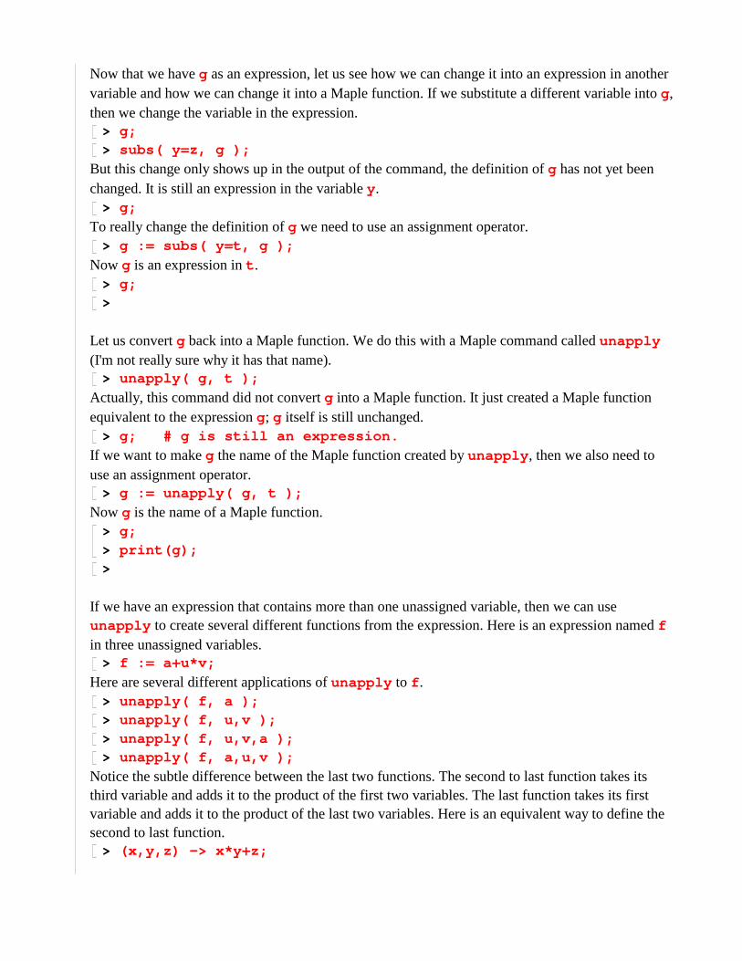
Now that we have g as an expression, let us see how we can change it into an expression in another variable and how we can change it into a Maple function. If we substitute a different variable into g, then we change the variable in the expression.

> g;> subs( y=z, g );

But this change only shows up in the output of the command, the definition of g has not yet been changed. It is still an expression in the variable y .

> g;

To really change the definition of g we need to use an assignment operator.> g := subs( y=t, g );

Now g is an expression in t .> g;>

Let us convert g back into a Maple function. We do this with a Maple command called unapply (I'm not really sure why it has that name).

> unapply( g, t );

Actually, this command did not convert g into a Maple function. It just created a Maple function equivalent to the expression g; g itself is still unchanged.

> g; # g is still an expression.

If we want to make g the name of the Maple function created by unapply , then we also need to use an assignment operator.

> g := unapply( g, t );

Now g is the name of a Maple function.> g;> print(g);>

If we have an expression that contains more than one unassigned variable, then we can use unapply to create several different functions from the expression. Here is an expression named f in three unassigned variables.

> f := a+u*v;

Here are several different applications of unapply to f .> unapply( f, a );> unapply( f, u,v );> unapply( f, u,v,a );> unapply( f, a,u,v );

Notice the subtle difference between the last two functions. The second to last function takes its third variable and adds it to the product of the first two variables. The last function takes its first variable and adds it to the product of the last two variables. Here is an equivalent way to define the second to last function.

> (x,y,z) -> x*y+z;

Here is an equivalent way to define the last function in the above list.> (x,y,z) -> x+y*z;

Be sure to convince yourself that these last two functions are equivalent to the functions returned by the last two unapply commands above.

>

Exercise: There are still other functions that could be defined from the expression f . Determine how many functions can be derived from f using unapply .

>

Exercise: Find an expression f in three variable from which we can define 15 different functions using unapply .

>

We have seen how to create an expression from a Maple function, and how to create a Maple function from an expression. Remember that creating an equivalent expression out of a Maple function is the only way to get most of Maple's symbolic manipulation commands to work on Maple functions. Creating an equivalent Maple function from an expression is something that is not done as often, but it is occasionally very useful.

>

>

4.6. Equations vs. functions: ambiguityEarlier in this worksheet we mentioned that mathematical formulas like the following one can be somewhat ambiguous.

= ( )g x − x2 1On the one hand it can be interpreted as the definition and naming of a function g. On the other hand, it can be interpreted as an equation. To see how this ambiguity might arise, suppose that we follow this formula with the next formula. (We did an example similar to this in Worksheet 2.)

= ( )g x − + 3 x2 x 5How should we interpret this second formula? Is it a redefinition of the function g, or is it a short hand notation for the following equation?

= − x2 1 − + 3 x2 x 5There is really no way to tell from the second formula itself which interpretation is correct. The cause of this ambiguity is that in standard mathematical notation, the equal sign has (at least) two distinct uses, as part of an assignment statement or as part of an equation. If the second formula above is meant to be a redefinition of the function g, then the equal sign in that formula is acting as part of an assignment statement. If on the other hand the second formula is meant to be a short hand for the third formula, then the equal sign in the second formula is acting as part of an equation. Let us translate these formulas into Maple and see what the two interpretations lead to. We will translate the first mathematical formula as the definition of a function g represented as a Maple function.

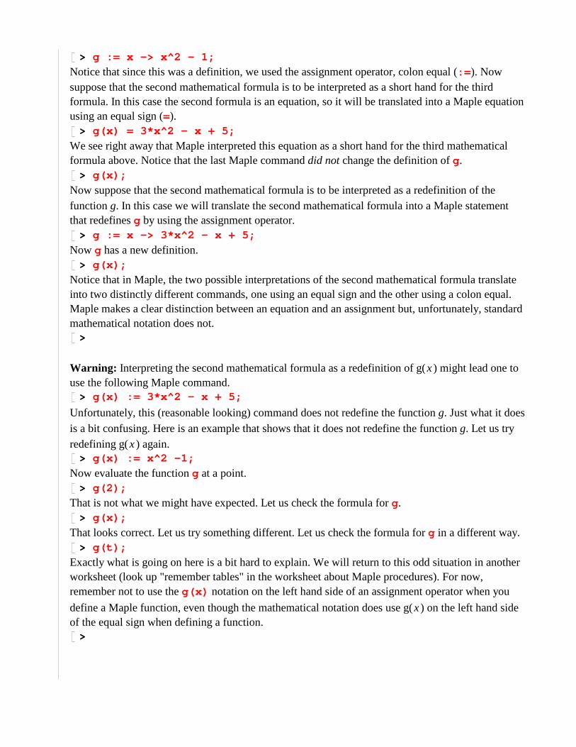
> g := x -> x^2 - 1;

Notice that since this was a definition, we used the assignment operator, colon equal (:= ). Now suppose that the second mathematical formula is to be interpreted as a short hand for the third formula. In this case the second formula is an equation, so it will be translated into a Maple equation using an equal sign (=).

> g(x) = 3*x^2 - x + 5;

We see right away that Maple interpreted this equation as a short hand for the third mathematical formula above. Notice that the last Maple command did not change the definition of g.

> g(x);

Now suppose that the second mathematical formula is to be interpreted as a redefinition of the function g. In this case we will translate the second mathematical formula into a Maple statement that redefines g by using the assignment operator.

> g := x -> 3*x^2 - x + 5;

Now g has a new definition.> g(x);

Notice that in Maple, the two possible interpretations of the second mathematical formula translate into two distinctly different commands, one using an equal sign and the other using a colon equal. Maple makes a clear distinction between an equation and an assignment but, unfortunately, standard mathematical notation does not.

>

Warning: Interpreting the second mathematical formula as a redefinition of ( )g x might lead one to use the following Maple command.

> g(x) := 3*x^2 - x + 5;

Unfortunately, this (reasonable looking) command does not redefine the function g. Just what it does is a bit confusing. Here is an example that shows that it does not redefine the function g. Let us try redefining ( )g x again.

> g(x) := x^2 -1;

Now evaluate the function g at a point.> g(2);

That is not what we might have expected. Let us check the formula for g.> g(x);

That looks correct. Let us try something different. Let us check the formula for g in a different way.> g(t);

Exactly what is going on here is a bit hard to explain. We will return to this odd situation in another worksheet (look up "remember tables" in the worksheet about Maple procedures). For now, remember not to use the g(x) notation on the left hand side of an assignment operator when you

define a Maple function, even though the mathematical notation does use ( )g x on the left hand side of the equal sign when defining a function.

>

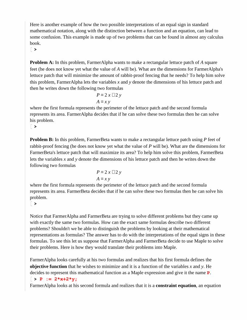
Here is another example of how the two possible interpretations of an equal sign in standard mathematical notation, along with the distinction between a function and an equation, can lead to some confusion. This example is made up of two problems that can be found in almost any calculus book.

>

Problem A: In this problem, FarmerAlpha wants to make a rectangular lettuce patch of A square feet (he does not know yet what the value of A will be). What are the dimensions for FarmerAlpha's lettuce patch that will minimize the amount of rabbit-proof fencing that he needs? To help him solve this problem, FarmerAlpha lets the variables x and y denote the dimensions of his lettuce patch and then he writes down the following two formulas = P + 2 x 2 y

= A x ywhere the first formula represents the perimeter of the lettuce patch and the second formula represents its area. FarmerAlpha decides that if he can solve these two formulas then he can solve his problem.

>

Problem B: In this problem, FarmerBeta wants to make a rectangular lettuce patch using P feet of rabbit-proof fencing (he does not know yet what the value of P will be). What are the dimensions for FarmerBeta's lettuce patch that will maximize its area? To help him solve this problem, FarmerBeta lets the variables x and y denote the dimensions of his lettuce patch and then he writes down the following two formulas = P + 2 x 2 y

= A x ywhere the first formula represents the perimeter of the lettuce patch and the second formula represents its area. FarmerBeta decides that if he can solve these two formulas then he can solve his problem.

>

Notice that FarmerAlpha and FarmerBeta are trying to solve different problems but they came up with exactly the same two formulas. How can the exact same formulas describe two different problems? Shouldn't we be able to distinguish the problems by looking at their mathematical representations as formulas? The answer has to do with the interpretations of the equal signs in these formulas. To see this let us suppose that FarmerAlpha and FarmerBeta decide to use Maple to solve their problems. Here is how they would translate their problems into Maple.

FarmerAlpha looks carefully at his two formulas and realizes that his first formula defines the objective function that he wishes to minimize and it is a function of the variables x and y. He decides to represent this mathematical function as a Maple expression and give it the name P.

> P := 2*x+2*y;

FarmerAlpha looks at his second formula and realizes that it is a constraint equation, an equation

that the variables x and y must satisfy. So FarmerAlpha translates this formula into a Maple equation, where he will give the constant A a value later on.

> A = x*y;>

Now it is FarmerBeta's turn to use Maple. Let us clear all the variables for him, so that he can start with a clean slate.

> restart;

FarmerBeta looks carefully at his two formulas and realizes that his first formula is a constraint equation, an equation that the variables x and y must satisfy. So FarmerBeta translates this formula into a Maple equation, where he will give the constant P a value later on.

> P = 2*x+2*y;

FarmerBeta looks at his second formula and realizes that it defines the objective function that he wishes to maximize and it is a function of the variables x and y. He decides to represent this mathematical function as a Maple expression and give it the name A.

> A := x*y;>

Now we see that, when translated into Maple, we can distinguish the two problems by looking at their Maple representations. The standard mathematical notation did not make a distinction between an assignment and an equation and that is why the two problems looked the same when represented mathematically. When you read a mathematics book you always need to be aware that an equal sign can be interpreted (at least) two ways and you always need to look carefully at the context that formulas are written in to decide which interpretation to give an equal sign.

>

Let us see how FarmerBeta would use Maple to finish solving his problem. First he needs to solve for one of the variables in the constraint equation. He decides to solve for y .

> solve( P=2*x+2*y, y );

Now he needs to take that solution and substitute it in for y in the objective function A.> subs( y=%, A );

This last expression needs to be differentiated, the derivative set to zero, and the resulting equation solved for x .

> solve( diff(%, x)=0, {x} );

And now he has the value for the variable x in terms of the constant P. To get the value for y he takes the value for x and substitutes it into the constraint equation and then solves for y .

> solve( subs(%, P=2*x+2*y), {y} );

The answer, of course, is that a square lettuce patch maximizes the area for a given amount of rabbit-proof fencing.

>

Exercise: Use Maple to solve FamerAlpha's problem.>

Exercise: Use Maple to solve FarmerBeta's problem again, but this time represent the objective function as a Maple function instead of as an expression.

>

>

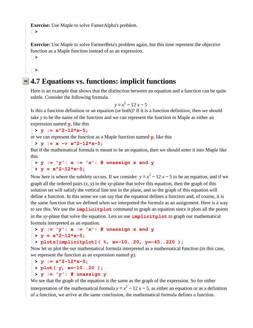
4.7 Equations vs. functions: implicit functionsHere is an example that shows that the distinction between an equation and a function can be quite subtle. Consider the following formula.

= y − − x2 12 x 5Is this a function definition or an equation (or both)? If it is a function definition, then we should take y to be the name of the function and we can represent the function in Maple as either an expression named y , like this

> y := x^2-12*x-5;

or we can represent the function as a Maple function named y , like this> y := x -> x^2-12*x-5;

But if the mathematical formula is meant to be an equation, then we should enter it into Maple like this

> y := 'y': x := 'x': # unassign x and y> y = x^2-12*x-5;

Now here is where the subtlety occurs. If we consider = y − − x2 12 x 5 to be an equation, and if we graph all the ordered pairs ( ,x y) in the xy-plane that solve this equation, then the graph of this solution set will satisfy the vertical line test in the plane, and so the graph of this equation will define a function. In this sense we can say that the equation defines a function and, of course, it is the same function that we defined when we interpreted the formula as an assignment. Here is a way to see this. We use the implicitplot command to graph an equation since it plots all the points

in the xy-plane that solve the equation. Lets us use implicitplot to graph our mathematical formula interpreted as an equation.

> y := 'y': x := 'x': # unassign x and y> y = x^2-12*x-5;> plots[implicitplot]( %, x=-10..20, y=-45..220 );

Now let us plot the our mathematical formula interpreted as a mathematical function (in this case, we represent the function as an expression named y ).

> y := x^2-12*x-5;> plot( y, x=-10..20 );> y := 'y': # unassign y

We see that the graph of the equation is the same as the graph of the expression. So for either

interpretation of the mathematical formula = y − − x2 12 x 5, as either an equation or as a definition of a function, we arrive at the same conclusion, the mathematical formula defines a function.

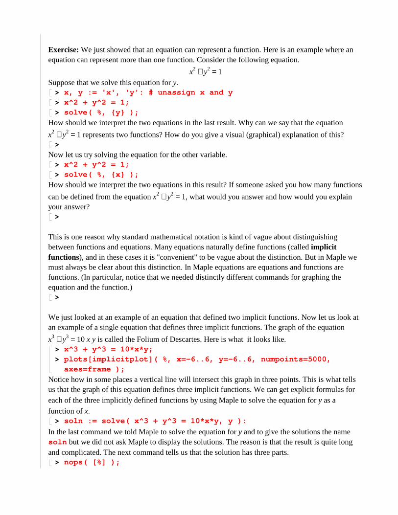
Exercise: We just showed that an equation can represent a function. Here is an example where an equation can represent more than one function. Consider the following equation.

= + x2 y2 1Suppose that we solve this equation for y.

> x, y := 'x', 'y': # unassign x and y> x^2 + y^2 = 1;> solve( %, {y} );

How should we interpret the two equations in the last result. Why can we say that the equation

= + x2 y2 1 represents two functions? How do you give a visual (graphical) explanation of this?>

Now let us try solving the equation for the other variable.> x^2 + y^2 = 1;> solve( %, {x} );

How should we interpret the two equations in this result? If someone asked you how many functions

can be defined from the equation = + x2 y2 1, what would you answer and how would you explain your answer?

>

This is one reason why standard mathematical notation is kind of vague about distinguishing between functions and equations. Many equations naturally define functions (called implicit functions), and in these cases it is "convenient" to be vague about the distinction. But in Maple we must always be clear about this distinction. In Maple equations are equations and functions are functions. (In particular, notice that we needed distinctly different commands for graphing the equation and the function.)

>

We just looked at an example of an equation that defined two implicit functions. Now let us look at an example of a single equation that defines three implicit functions. The graph of the equation

= + x3 y3 10 x y is called the Folium of Descartes. Here is what it looks like.> x^3 + y^3 = 10*x*y;> plots[implicitplot]( %, x=-6..6, y=-6..6, numpoints=5000,

axes=frame );

Notice how in some places a vertical line will intersect this graph in three points. This is what tells us that the graph of this equation defines three implicit functions. We can get explicit formulas for each of the three implicitly defined functions by using Maple to solve the equation for y as a function of x.

> soln := solve( x^3 + y^3 = 10*x*y, y ):

In the last command we told Maple to solve the equation for y and to give the solutions the name soln but we did not ask Maple to display the solutions. The reason is that the result is quite long and complicated. The next command tells us that the solution has three parts.

> nops( [%] );

Here is the first part of the solution, which is the formula for one of the implicitly defined functions.> soln[1];

Here is the formula for one of the other implicitly defined functions.> soln[2];

The following execution group graphs each of the three implicitly defined functions but it displays them together in a single graph. The three implicit functions are each given a different color. We can see from this graph how the three implicit functions fit together to build up the graph of the equation.

> p1:=plot(soln[1], x=-6..6, view=[-6..6,-6..6], axes=frame, color=blue):

> p2:=plot(soln[2], x=-6..6, view=[-6..6,-6..6], axes=frame, color=red):

> p3:=plot(soln[3], x=-6..6, view=[-6..6,-6..6], axes=frame, color=green):

> plots[display](p1,p2,p3);

Notice how each implicit function by itself satisfies the vertical line test. And notice how the dividing points between the different implicit functions is exactly where the graph of the equation has vertical tangent lines. These are exactly the points where the graph of the equation stops satisfying the vertical line test.

>

Exercise: Consider the following equation.

= − − y4

4

9 y2

2x 0

Here is what the graph of this equation looks like.> (y^4)/4 - (9/2)*y^2 - x = 0;> plots[implicitplot]( %, x=-20..20, y=-6..6 );

We want to consider the question of how many (implicit) functions are defined by this equation. Looking at the graph, how many functions with y as a function of x do you think are defined by the equation? How many functions with x as a function of y do you think are defined by the equation? Now consider the results of the following two solve commands.

> solve( (1/4)*y^4-(9/2)*y^2-x=0, {y} );> solve( (1/4)*y^4-(9/2)*y^2-x=0, {x} );

Explain how these results relate to the above graph of the equation.>

Exercise: Consider the following equation.

= x2 − + y3 6 y2 9 yHere is what the graph of this equation looks like.

> x^2 = y^3 - 6*y^2 + 9*y;> plots[implicitplot]( %, x=-3..3, y=-1..5, grid=[100,100] );

We want to consider the question of how many (implicit) functions are defined by this equation.

Looking at the graph, how many functions with y as a function of x do you think are defined by the equation? How many functions with x as a function of y do you think are defined by the equation? Now consider the results of the following two solve commands.

> solve( x^2=y^3-6*y^2+9*y, {x} );> solve( x^2=y^3-6*y^2+9*y, {y} );

Explain how these results relate to the above graph of the equation.>

>

4.8. Piecewise defined functionsNow we will see how to define "piecewise-defined" functions in Maple. Piecewise-defined functions are functions that are defined by different formulas at different parts of the function's domain. In other words, the definition of a piecewise defined function comes in several pieces. Probably the most well known piecewise defined function is the absolute value function.

= x�

�

−x < x 0 x ≤ 0 x

This tells us that if x is a negative number, then we negate it (to get a positive number) and if x is positive, then we just leave it alone.

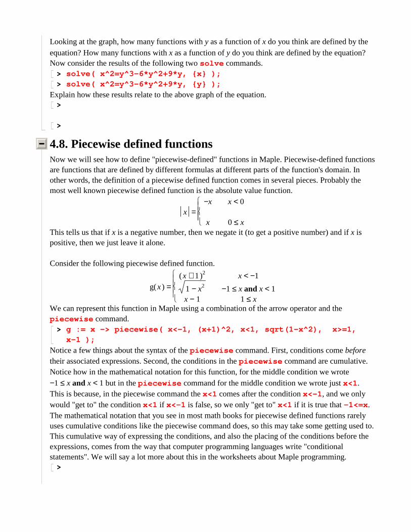
Consider the following piecewise defined function.

= ( )g x

�

�

( ) + x 1 2 < x −1

− 1 x2 and ≤ −1 x < x 1 − x 1 ≤ 1 x

We can represent this function in Maple using a combination of the arrow operator and the piecewise command.

> g := x -> piecewise( x<-1, (x+1)^2, x<1, sqrt(1-x^2), x>=1, x-1 );

Notice a few things about the syntax of the piecewise command. First, conditions come before their associated expressions. Second, the conditions in the piecewise command are cumulative. Notice how in the mathematical notation for this function, for the middle condition we wrote

and ≤ −1 x < x 1 but in the piecewise command for the middle condition we wrote just x<1 . This is because, in the piecewise command the x<1 comes after the condition x<-1 , and we only would "get to" the condition x<1 if x<-1 is false, so we only "get to" x<1 if it is true that -1<=x . The mathematical notation that you see in most math books for piecewise defined functions rarely uses cumulative conditions like the piecewise command does, so this may take some getting used to. This cumulative way of expressing the conditions, and also the placing of the conditions before the expressions, comes from the way that computer programming languages write "conditional statements". We will say a lot more about this in the worksheets about Maple programming.

>

If we call the piecewise function by itself (that is, without using the arrow notation), we get a "piecewise expression", and the expression is nicely typeset. Notice that this looks just like the mathematical notation for the function, except for the cumulative use of the conditions.

> piecewise( x<-1, (x+1)^2, x<1, sqrt(1-x^2), x>=1, x-1 );

If we convert g into an expression by evaluating g at an unassigned variable, we get the same "piecewise expression".

> a := 'a':> g(a);

If we evaluate the name g, we do not get much information.> g;

Here is how we get the full definition of g.> eval( g );

If we evaluate g at a number, then we get the value of the function.> g(4); > g(-3); > g(0);>

Exercise: Verify each of the last three results by evaluating yourself, by hand, the apropriate parts of the definition of g.

>

We can graph g like any other Maple function.> plot( g, -2..2, scaling=constrained );

(Try graphing g without the option scaling=constrained .)>

Let us add another condition to the domain of g.> g2 := x -> piecewise( x<-1, (x+1)^2, x<1, sqrt(1-x^2), x<3,

x-1, x>=3, 3*(x-3)+2 );

> g2(x);> plot( g2, -2..4 );>

Piecewise expressions can be used in almost exactly the same way as we would use other expressions. Here is a simple example.

> h := piecewise( x<1, x*(1-x), x>=1, (1-x)*(2-x) );

We can ask Maple to differentiate this expression.> diff( h, x );

We can use this expression in other expressions.> exp(x*h)*h;

We can even ask Maple to simplify this last result.> simplify( % );

We can evaluate the expression at a point, but here we need to be careful. The subs command will give strange results.

> subs( x=1/2, h );

That is not what we wanted (can you see what happened?). In a later worksheet we will be able to explain why the subs command produced this result. For evaluating a piecewise expression at a point, the eval command should be used instead of subs .

> eval( h, x=1/2 );>

Exercise: Define the following two functions (as expressions).> f := piecewise( x<1, 4*x*(1-x), x>=1, 4*(1-x)*(2-x) );> g := sin(Pi*x);

In the following graph, identify which graph is from which function.> plot( [f,g], x=0..2 );

These two graphs demonstrate how strikingly similar a sine curve and a parabola can be. Try "zooming in" on the domain from zero to one. It is also interesting to graph the derivatives of these two functions.

> df := diff( f, x );> dg := diff( g, x );> plot( [df,dg], x=0..2 );

Notice that the derivatives are not at all hard to distinguish.>

Exercise: Explain why the following two piecewise defined functions are really the same function.> f := x -> piecewise( x<0, x, x<=5, 2*x, x>5, -x+15 );> g := x -> piecewise( x>5, -x+15, x>=0, 2*x, x<0, x );> f(x);> g(x);>

Exercise: Suppose we are given the following piecewise defined function.> f := x -> piecewise( x< -1, 2*x, x<= 1, x^2, x<=3, 1/x, x>3,

ln(x) );> f(x);

Fill in the missing conditions in the following definition of g so that g is equivalent to f .> g := x -> piecewise( ???, ln(x), ???, 1/x, ???, x^2, ???, 2*x

);>

Exercise: Define and then graph a piecewise defined function that is parabolic for x less than or

equal to zero and is a hyperbola for x strictly greater than zero.>

>

4.9 Plot valued functionsThe purpose of this section is twofold. First, to show you how useful the concept of a function is and how versatile Maple functions are. Second, to show you a specific technique that we will use for creating animations in Maple. What we want to do is create a function whose output, for a given input, is a graph that depends in some way on the input to the function. In other words, we shall create "plot valued functions".

Consider the following simple example.> p := t -> plot( x^2+t, x=-5..5, -5..5 );

We have defined a Maple function that takes a single number as its input, which is denoted by t, and

the value of the function is a plot command that draws a graph of the function + x2 t. Notice two things about this definition of the function p. First, the plot command was not executed when we defined the function. The plot command will not be executed until we evaluate this function with some input. Second, the input to the function p is a parameter of the function that plot is supposed to graph. When we evaluate the plot valued function at a point, say p(-3) , the input -3 becomes

the parameter in the function being graphed, in this case − x2 3.> p(-3);

If we evaluate this function at a different input, we get a different graph.> p(1);

Notice that the function p will give us an error if we try to evaluate it with a symbolic input. The plot command that is the value of p will not work unless the parameter t is given a numeric value.

> p(z);>

We can use a function like p to create an animation. An animation in Maple is a sequence of graphs displayed one after the other in fairly quick order to create the illusion of movement. To use the function p to create an animation we first use p along with the seq command to create a sequence of graphs. The following seq command causes the index variable n to increment through the integers from -10 to 10 . This causes the input parameter to p to increment from -1 to 1 in steps of 1/10. For each of these 21 different input parameters (why 21?), p is evaluated to a graph. We put a colon at the end of the following command because we are not yet ready to view the 21 graphs created by this command.

> frames := seq( p(n/10), n=-10..10 ):

The last command created, but did not display, a sequence of 21 graphs. The result of the command was given the name frames because each graph in this sequence is called a frame of the

animation. Each frame is a graph of the function + x2 t but each frame has a different value for the

parameter t, so each frame looks slightly different from any other frame. The animation will display

these frames in very quick succession and show the graphs of the functions + x2 t as t increases from -1 to 1, so we will see a parabola moving up.

Now we use the display command with the insequence=true option to tell Maple to display this sequence of graphs in quick order and create an animation. To see the animation, click on the graph generated by the next command and then click on the "play" button in the animation context bar at the top of the Maple window. You can also step through the individual frames of the animation by repeatedly clicking on the button just to the right of the play button.

> plots[display]( [frames], insequence=true );>

Exercise: What happens if we remove the insequence=true option from the display command in the last example?

>

Here is an example of a plot valued function in which the parameter of the function changes the range of the plot.

> p := t -> plot( x^2, x=-1-t..1+t );

The following seq command creates 41 graphs with the input to the plot valued function p

incrementing from 0 to 4 in steps of 1/10 (so the ranges of the graphs change from .. −1 1 to .. −5 5). The display command creates an animation from these 41 graphs.

> seq( p(n/10), n=0..40 ):> plots[display]( [%], insequence=true );>

Sometimes it is desirable to put a "background image" into an animation. A background image is a part of every frame of the animation that does not change from frame to frame. Let us redo the last animation with a background image that is a fixed parabola. Here is the plot valued function.

> p := t -> plot( x^2, x=-1-t..1+t, view=[-5..5, 0..25] );

Now we define the sequence of frames and create the animation. But notice that this time we give the animation a name (a for "animation") and do not show it yet (notice the colon at the end of the display command).

> seq( p(n/10), n=0..40 ):> a := plots[display]( [%], insequence=true ):

Now define the background image. We also give this graph a name (b for background) and do not show it yet.

> b := plot( x^2+.5, x=-5..5, color=blue, view=[-5..5, 0..25] ):

Now here is the command that combines the animation with the background image.> plots[display]( {a,b} );>

Here is an example of a plot valued function in which the function's parameter changes both the function being plotted and the range of each plot.

> p := c -> plot( -x^2+c, x=-sqrt(c)..sqrt(c), ytickmarks=[1,2,3,4] );

> seq( p(1+n/10), n=0..30 ):> plots[display]( [%], insequence=true );>

Exercise: In the last plot valued function, explain exactly how the input c to the function p affects the graph being drawn by p.

>

In the last example, the parameter of the plot valued function controlled two parameters of the graph. Here is a way to do the same thing which makes it more explicit that we are controlling two aspects of the graph. We make the plot valued function a function of two variables and make each input variable control just one aspect of the graph.

> p := (t,c) -> plot( -x^2+t, x=-sqrt(c)..sqrt(c), ytickmarks=[1,2,3,4] );

The first parameter of the plot valued function determines how much the parabola is shifted vertically and the second parameter determines the horizontal range of the graph. This plot valued function may have two inputs, but when we go to create an animation, the animation really only has one parameter, "time". So when we use the seq command to create the sequence of frames, we need to use the single index variable from the seq command in both inputs to the plot valued function.

> seq( p(1+n/10, 1+n/10), n=0..30 ):> plots[display]( [%], insequence=true );

But now we are also able to make p's two input variables vary in independent ways. The following animation makes the parabola rise but the horizontal range for the parabola will shrink to zero as the animation evolves.

> seq( p(1+n/10, 4-n*399/3000), n=0..30 ):> plots[display]( [%], insequence=true );

Notice how, with the same plot valued function, we were able to create two fairly different animations. By explicitly having one input variable for each aspect of the graph that we want to control, we gain more flexibility compared to having a single input variable control more than one aspect of the graph.

>

Exercise: In the last example, change the 399 to 400 . This will cause an error message. Explain why.

>

Here is an animation that uses a third parameter in the plot valued function to combine ideas from the previous two animations. This animation also has a background image that is the initial position

of the moving parabola.> p := (t,c,d) -> plot( -x^2+t, x=-sqrt(c)..sqrt(d),

view=[-2..2,0..4] ):> seq( p(1+n/10, 1+n/10, 1-n/30), n=0..30 ):> a := plots[display]( [%], insequence=true ):> b := plot( -x^2+1, x=-1..1, view=[-2..2,0..4] ):> plots[display]( {a,b}, ytickmarks=[1,2,3,4] );>

Exercise: Remove the view option from the definition of b and see what happens to the animation. Then put the view option back in b and remove the view option from the definition of p and see what happens. This shows that display sometimes needs some hints about how it should combine graphs with different horizontal or vertical ranges.

>

We will make use of plot valued functions many times in future worksheets to create animations. In the next worksheet we will see that Maple has two commands for animating graphs of functions, animate and animatecurve , but these two commands have limitations in the kinds of animations that they can create. Plot valued functions along with the seq and display command can be used to create animations that surpass the limitations of animate and animatecurve .

>

Exercise: Use a plot valued function with the seq and display commands to create an animation of the sine function being shifted horizontally until it becomes the sine function again. Start the animation with the sine function graphed between 0 and 2π and end the animation with the sine function graphed between 0 and 4π. Your animation should contain at least 20 frames.

>

Exercise: Use a plot valued function with the seq and display commands to create an animation

of the function ( )sin t increasing its period until it becomes the function �

���

�

���sin

t

4. Start the animation

with the ( )sin t graphed between 0 and 2π and end the animation with the �

���

�

���sin

t

4 graphed between

0 and 8π. Your animation should contain at least 20 frames.>

Exercise: The goal of this exercise is to find an interesting connection between the following three equations.

= + x y 1

= + x2 y2 1 = ( )max ,x y 1.

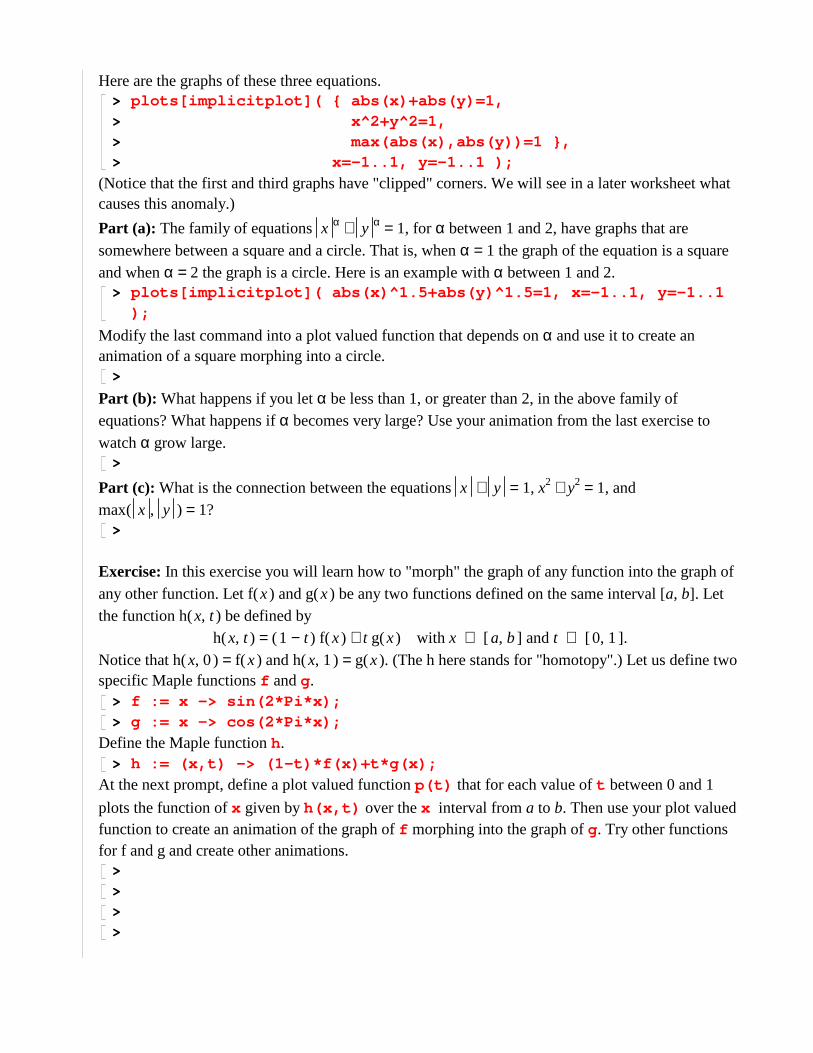
Here are the graphs of these three equations.> plots[implicitplot]( { abs(x)+abs(y)=1, > x^2+y^2=1,> max(abs(x),abs(y))=1 }, > x=-1..1, y=-1..1 );

(Notice that the first and third graphs have "clipped" corners. We will see in a later worksheet what causes this anomaly.)

Part (a): The family of equations = + x α y α 1, for α between 1 and 2, have graphs that are somewhere between a square and a circle. That is, when = α 1 the graph of the equation is a square and when = α 2 the graph is a circle. Here is an example with α between 1 and 2.

> plots[implicitplot]( abs(x)^1.5+abs(y)^1.5=1, x=-1..1, y=-1..1 );

Modify the last command into a plot valued function that depends on α and use it to create an animation of a square morphing into a circle.

>

Part (b): What happens if you let α be less than 1, or greater than 2, in the above family of equations? What happens if α becomes very large? Use your animation from the last exercise to watch α grow large.

>

Part (c): What is the connection between the equations = + x y 1, = + x2 y2 1, and = ( )max ,x y 1?

>

Exercise: In this exercise you will learn how to "morph" the graph of any function into the graph of any other function. Let ( )f x and ( )g x be any two functions defined on the same interval [ ,a b]. Let the function ( )h ,x t be defined by

= ( )h ,x t + ( ) − 1 t ( )f x t ( )g x with ∈ x [ ],a b and ∈ t [ ],0 1 .Notice that = ( )h ,x 0 ( )f x and = ( )h ,x 1 ( )g x . (The h here stands for "homotopy".) Let us define two specific Maple functions f and g.

> f := x -> sin(2*Pi*x);> g := x -> cos(2*Pi*x);

Define the Maple function h.> h := (x,t) -> (1-t)*f(x)+t*g(x);

At the next prompt, define a plot valued function p(t) that for each value of t between 0 and 1

plots the function of x given by h(x,t) over the x interval from a to b. Then use your plot valued function to create an animation of the graph of f morphing into the graph of g. Try other functions for f and g and create other animations.

> > > >

>

4.10. Vector valued functionsThe most basic functions that we study in mathematics are the real valued functions of one real variable. These functions have as their input one number and as their output another number. These are the functions that occupy us during most of first and second semester calculus. This is also the kind of function that we have been using for most of our examples in these worksheets. In these worksheets we have sometimes also used examples of real valued multivariate functions. These are functions of several real variables, that is, functions whose input is two or more numbers and whose output is a single number. These are the functions that are studied mostly in third semester calculus where one learns about partial derivatives and double and triple integrals. Real valued multivariate functions are sometimes referred to as scalar functions (or scalar fields).

In this section we want to look at how Maple can represent vector valued functions. These are functions that have two or more numbers as their output. We look at both vector valued functions of a single real variable (also called parametric curves) and multivariate vector valued functions. Parametric curves (i.e., vector valued functions of a single real variable) are, as their name implies, used to model curves in the plane and in space. These kinds of functions are usually first introduced in first or second semester calculus and they play a big role in vector calculus. The class of multivariate vector valued functions is huge and has many applications. Some examples of multivariate vector valued functions that you may have already studied are parametric surfaces in space, vector fields in the plane and in space, and matrix transformations in linear algebra.

Before showing how to represent vector valued functions in Maple, let us quickly review how Maple represents the other kinds of functions. The real valued functions of a real variable are represented as either Maple functions of one variable or as expressions in one variable.

> f := x -> x^2;

or> f := x^2;

Notice that Maple functions, since they identify the independent variable, have the advantage of allowing for unambiguous parameters in the definition of the function. So for example

> f := x -> y*x^2;

is unambiguously a (quadratic) function of one variable. But the expression> f := y*x^2;

can be ambiguous about what it represents.>

Multivariate functions are represented in Maple as Maple functions of several variables or as expressions in several variables.

> g := (x,y) -> y*x^2;

or

> g := y*x^2;

Notice how the Maple function g is completely distinguished from the last version of the Maple function f . But the expression g cannot really be distinguished from the last definition of the expression f .

>

Multivariate functions of more than two variables are easy to represent.> h := (x,y,z,t) -> x^2+y^2+z^2-t^2;

or> h := x^2+y^2+z^2-t^2;>

Now we can look at an example of a vector valued function. First we will represent a 2-dimensional vector valued function of a single real variable, and we will represent it using expressions. For any given number as an input, our function needs to compute two numbers as the output. Each output number needs an expression to express the rule for computing it. We call these expressions the component functions of the vector valued function. The vector valued function is defined by putting the component functions in a list inside square brackets.

> f := [t^3-2*t, t^2-t];

If we want to, we can define the component functions first, and then define the vector valued function in terms of the component functions. Notice that each component function is a real valued function of a single variable.

> f1 := t^3-2*t;> f2 := t^2-t;> f := [f1, f2];

Using standard mathematical notation, this vector valued function can be expressed in a variety of ways. For example

= ( )f t ( ), − t3 2 t − t2 tor

= ( )f t ( ),( )f1 t ( )f2 t where = ( )f1 t − t3 2 t and = ( )f2 t − t2 tor even

= x − t3 2 t and = y − t2 t.

Now that we have a representation of a vector valued function, let us see how we can work with it. We can evaluate our function at a point using either the eval or subs command.

> eval( f, t=2 );> subs( t=2, f );

We can differentiate our function using the diff command.> diff( f, t );

Notice that the derivative is computed componentwise and the derivative of this vector valued function is another vector valued function.

>

Let us try to compose this vector valued function with some other function. If we want a composition of the form ( )h ( )f x then we need a multivariate function h that takes two input numbers (why?). We will use the following definition for our h.

> h := x+y;

Now we can compute the composition.> subs( x=f1,y=f2, h );> eval( h, {x=f1,y=f2} ); # notice the braces

Notice two things. We needed to refer to the component functions f1 and f2 to do the composition;

we could not refer to the function f by its name. And the function ( )h ( )f x is a real valued function of a single variable.

>

Let us try to graph our vector valued function.> plot( f, t=-3/2..2 );

Wait, that is not correct! The last command did not draw the graph of our vector valued function f . Instead, the plot command simply interpreted f as a list of two real valued functions of a real variable, and so it drew two graphs, one for each component function. How do we get the plot command to interpret f as one (vector valued) function? The answer to this is messy. One way is to use the component functions f1 and f2 in the following syntax of the plot command. Notice that the range for the independent variable needs to be inside the brackets with the component functions.

> plot( [f1, f2, t=-3/2..2] );

This is the graph of our function f , it is a curve in the plane (remember, vector valued functions of a single variable are also called "parametric curves").

>

The other way to get the plot command to graph the function f is to define f using a slightly different syntax. Instead of putting the component functions in a list inside of brackets, put the component functions inside of parentheses.

> f := (f1, f2);

Now put f in the plot command using the following syntax.> plot( [f, t=-3/2..2] );

At least we were able to graph f by referring to it by name rather than having to refer to the names of the component functions. But now we have a different problem!

> diff( f, t );

Now the diff command does not work. We need to put brackets around f in the diff command.> diff( [f], t );

And evaluating the function using subs needs to be changed also.> subs( t=2, f );> subs( t=2, [f] );

Using eval works though.> eval( f, t=2 );

As we will see several times in this section, Maple unfortunately does not have a consistent syntax for defining and using vector valued functions. Of the two syntaxes given just above, the first one is preferable since it works better with the diff and subs commands.

>

Now we shall turn to representing our vector valued function using Maple functions. There are two reasonable ways to do this and they have to do with slightly different ways of thinking about the vector valued function. One way thinks of the vector valued function as a function that takes in one number and outputs two numbers. The second way thinks of the vector valued function as being made up of two real valued component functions. These two ways of thinking lead to the following two representations that we will call g1 and g2 .

> g1 := t->(t^3-2*t, t^2-t);> g2 := [t->t^3-2*t, t->t^2-t];

Notice the subtle differences in these two definitions. The first representation is somewhat analogous to the mathematical notation

= ( )f t ( ), − t3 2 t − t2 t .The second representation is more analogous to the mathematical notation.

= ( )f t ( ),( )f1 t ( )f2 t where = ( )f1 t − t3 2 t and = ( )f2 t − t2 t.As we will now show, each of these Maple representations has advantages and disadvantages. Let us see how we can work with them.

>

With either representation, we can use functional notation to evaluate the function.> g1(2);> g2(2);>

We should be able to use the D operator to differentiate the function.> D( g1 );> D( g2 );

The D operator only worked on the second representation, g2 .>

Let us try composition. Here is a function we can compose with.> h := (x,y) -> x+y;

We should be able to use the @ operator to do the composition with h.> (h@g1)(z);> (h@g2)(z);

The @ operator only worked on the first representation, g1 (and the D operator only worked on g2 !).>

There is a second way to do the composition. We should be able to compose h with the vector

valued function using functional notation.> h(g1(z));> h(g2(z));

Again, this only worked with the first representation.>

What about graphing the vector valued function? To make a long story short, neither representation will work with the plot command because it needs the component functions and the range all together inside a pair of brackets.

> plot( [t->t^3-2*t, t->t^2-t, -3/2..2] );>

Maple's documentation is unclear about how vector valued functions should be represented using the arrow notation. The following help page implies that the way we defined g1 is the "correct syntax" for vector valued functions, but we saw that g1 did not work with the D operator nor with the plot command.

> ?operators,functional

On the other hand, the way we defined g2 worked with the D operator and, as we will see in the next example, the way we defined g2 does work with the plot3d command (but the way we defined g1 does not). But g2 does not work with composition. And to make things even more confusing, if we use unapply to convert the expression version of the function f into a Maple function, then we get neither g1 nor g2 .

> unapply( f, t );

So it seems that there is no preferred way in Maple to define vector valued functions using the arrow notation. From a mathematical point of view, the two ways of thinking about vector valued functions that lead to the two ways of using the arrow notation are both valid, and so both uses of the arrow notation are reasonable. In any given situation we need to pick the representation that works best.

>

Exercise: There are two other ways to represent our vector valued function using Maple functions.> g3 := t->[t^3-2*t, t^2-t];> g4 := (t->t^3-2*t, t->t^2-t);

In each representation we have switched parentheses and brackets. Play around with these two representations and see how they work with respect to evaluation, differentiation, composition, and graphing. (For example, g4 works reasonably well with the plot command.) Notice that g3 was the result of the unapply command just above.

>

Exercise: Here are two more ways to define a vector valued function, motivated by an example from this help page. These two ways use Maple's notation for vectors, which is used in the VectorCalculus package. Here is a vector valued function written first as an expression and then as a

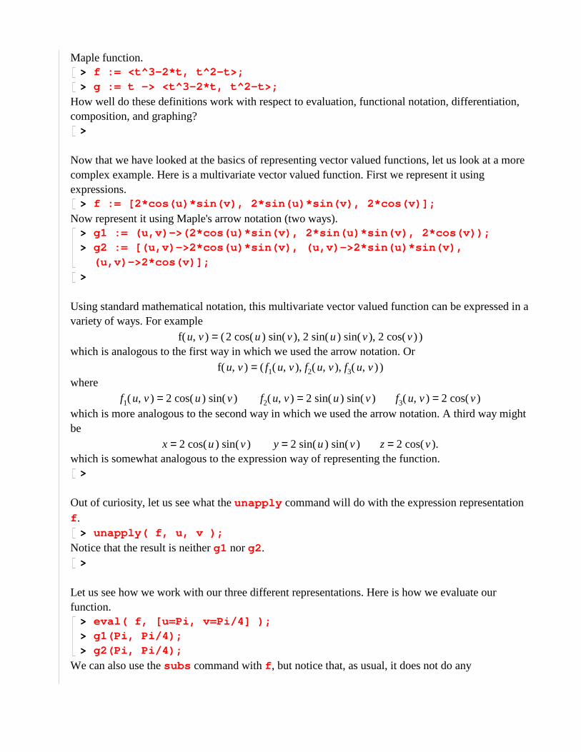
Maple function.> f := <t^3-2*t, t^2-t>;> g := t -> <t^3-2*t, t^2-t>;

How well do these definitions work with respect to evaluation, functional notation, differentiation, composition, and graphing?

>

Now that we have looked at the basics of representing vector valued functions, let us look at a more complex example. Here is a multivariate vector valued function. First we represent it using expressions.

> f := [2*cos(u)*sin(v), 2*sin(u)*sin(v), 2*cos(v)];

Now represent it using Maple's arrow notation (two ways).> g1 := (u,v)->(2*cos(u)*sin(v), 2*sin(u)*sin(v), 2*cos(v));> g2 := [(u,v)->2*cos(u)*sin(v), (u,v)->2*sin(u)*sin(v),

(u,v)->2*cos(v)];>

Using standard mathematical notation, this multivariate vector valued function can be expressed in a variety of ways. For example

= ( )f ,u v ( ), ,2 ( )cos u ( )sin v 2 ( )sin u ( )sin v 2 ( )cos vwhich is analogous to the first way in which we used the arrow notation. Or

= ( )f ,u v ( ), ,( )f1 ,u v ( )f2 ,u v ( )f3 ,u vwhere

= ( )f1 ,u v 2 ( )cos u ( )sin v = ( )f2 ,u v 2 ( )sin u ( )sin v = ( )f3 ,u v 2 ( )cos vwhich is more analogous to the second way in which we used the arrow notation. A third way might be

= x 2 ( )cos u ( )sin v = y 2 ( )sin u ( )sin v = z 2 ( )cos v .which is somewhat analogous to the expression way of representing the function.

>

Out of curiosity, let us see what the unapply command will do with the expression representation f .

> unapply( f, u, v );

Notice that the result is neither g1 nor g2 .>

Let us see how we work with our three different representations. Here is how we evaluate our function.

> eval( f, [u=Pi, v=Pi/4] );> g1(Pi, Pi/4);> g2(Pi, Pi/4);

We can also use the subs command with f , but notice that, as usual, it does not do any

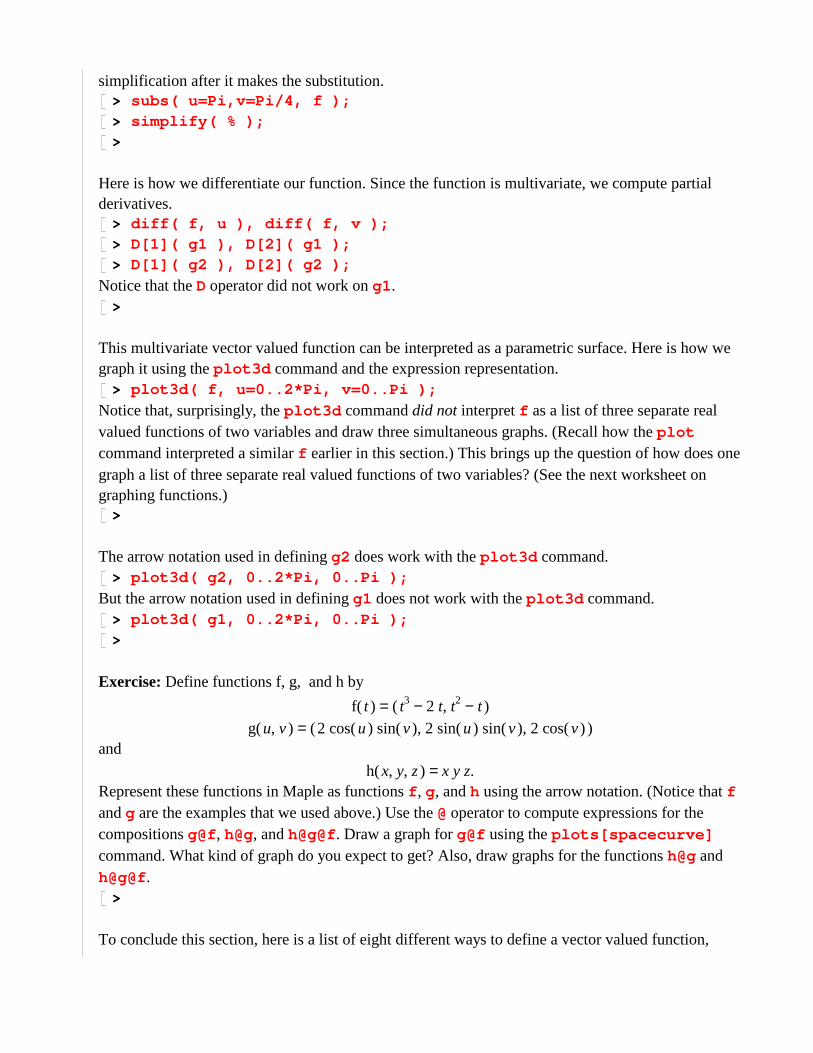
simplification after it makes the substitution.> subs( u=Pi,v=Pi/4, f );> simplify( % );>

Here is how we differentiate our function. Since the function is multivariate, we compute partial derivatives.

> diff( f, u ), diff( f, v );> D[1]( g1 ), D[2]( g1 );> D[1]( g2 ), D[2]( g2 );

Notice that the D operator did not work on g1 .>

This multivariate vector valued function can be interpreted as a parametric surface. Here is how we graph it using the plot3d command and the expression representation.

> plot3d( f, u=0..2*Pi, v=0..Pi );

Notice that, surprisingly, the plot3d command did not interpret f as a list of three separate real valued functions of two variables and draw three simultaneous graphs. (Recall how the plot command interpreted a similar f earlier in this section.) This brings up the question of how does one graph a list of three separate real valued functions of two variables? (See the next worksheet on graphing functions.)

>

The arrow notation used in defining g2 does work with the plot3d command.> plot3d( g2, 0..2*Pi, 0..Pi );

But the arrow notation used in defining g1 does not work with the plot3d command.> plot3d( g1, 0..2*Pi, 0..Pi );>

Exercise: Define functions f, g, and h by

= ( )f t ( ), − t3 2 t − t2 t

= ( )g ,u v ( ), ,2 ( )cos u ( )sin v 2 ( )sin u ( )sin v 2 ( )cos vand

= ( )h , ,x y z x y z.Represent these functions in Maple as functions f , g, and h using the arrow notation. (Notice that f and g are the examples that we used above.) Use the @ operator to compute expressions for the compositions g@f, h@g, and h@g@f. Draw a graph for g@f using the plots[spacecurve] command. What kind of graph do you expect to get? Also, draw graphs for the functions h@g and h@g@f.

>

To conclude this section, here is a list of eight different ways to define a vector valued function,

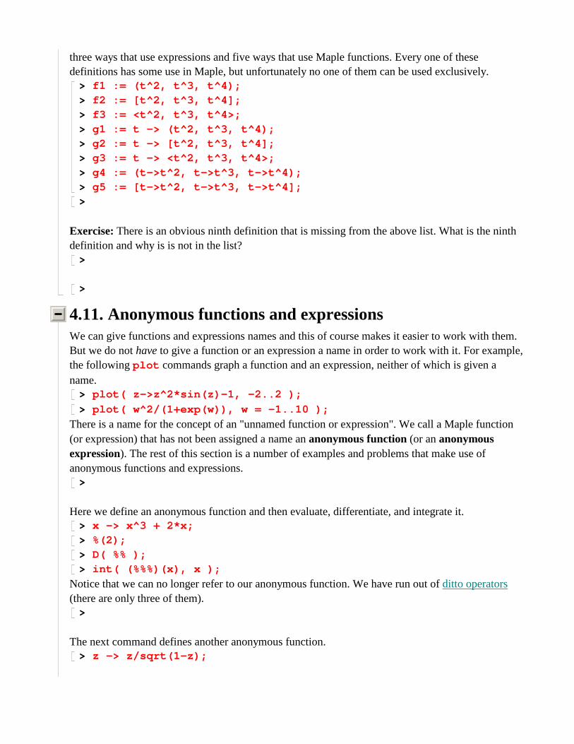
three ways that use expressions and five ways that use Maple functions. Every one of these definitions has some use in Maple, but unfortunately no one of them can be used exclusively.

> f1 := (t^2, t^3, t^4);> f2 := [t^2, t^3, t^4];> f3 := <t^2, t^3, t^4>;> g1 := t -> (t^2, t^3, t^4);> g2 := t -> [t^2, t^3, t^4];> g3 := t -> <t^2, t^3, t^4>;> g4 := (t->t^2, t->t^3, t->t^4);> g5 := [t->t^2, t->t^3, t->t^4];>

Exercise: There is an obvious ninth definition that is missing from the above list. What is the ninth definition and why is is not in the list?

>

>

4.11. Anonymous functions and expressionsWe can give functions and expressions names and this of course makes it easier to work with them. But we do not have to give a function or an expression a name in order to work with it. For example, the following plot commands graph a function and an expression, neither of which is given a name.

> plot( z->z^2*sin(z)-1, -2..2 );

> plot( w^2/(1+exp(w)), w = -1..10 );

There is a name for the concept of an "unnamed function or expression". We call a Maple function (or expression) that has not been assigned a name an anonymous function (or an anonymous expression). The rest of this section is a number of examples and problems that make use of anonymous functions and expressions.

>

Here we define an anonymous function and then evaluate, differentiate, and integrate it.> x -> x^3 + 2*x;> %(2);> D( %% );> int( (%%%)(x), x );

Notice that we can no longer refer to our anonymous function. We have run out of ditto operators (there are only three of them).

>

The next command defines another anonymous function.> z -> z/sqrt(1-z);

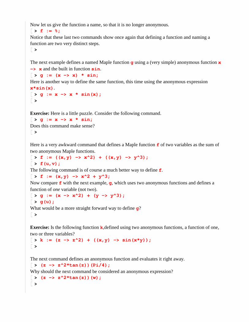
Now let us give the function a name, so that it is no longer anonymous.> f := %;

Notice that these last two commands show once again that defining a function and naming a function are two very distinct steps.

>

The next example defines a named Maple function g using a (very simple) anonymous function x

-> x and the built in function sin .> g := (x -> x) * sin;

Here is another way to define the same function, this time using the anonymous expression x*sin(x) .

> g := x -> x * sin(x);>

Exercise: Here is a little puzzle. Consider the following command.> g := x -> x * sin;

Does this command make sense?>

Here is a very awkward command that defines a Maple function f of two variables as the sum of two anonymous Maple functions.

> f := ((x,y) -> x^2) + ((x,y) -> y^3);> f(u,v);

The following command is of course a much better way to define f .> f := (x,y) -> x^2 + y^3;

Now compare f with the next example, g, which uses two anonymous functions and defines a function of one variable (not two).

> g := (x -> x^2) + (y -> y^3);> g(u);

What would be a more straight forward way to define g?>

Exercise: Is the following function k ,defined using two anonymous functions, a function of one, two or three variables?

> k := (z -> z^2) + ((x,y) -> sin(x*y));>

The next command defines an anonymous function and evaluates it right away.> (z -> z^2*tan(z))(Pi/4);

Why should the next command be considered an anonymous expression?> (z -> z^2*tan(z))(w);>

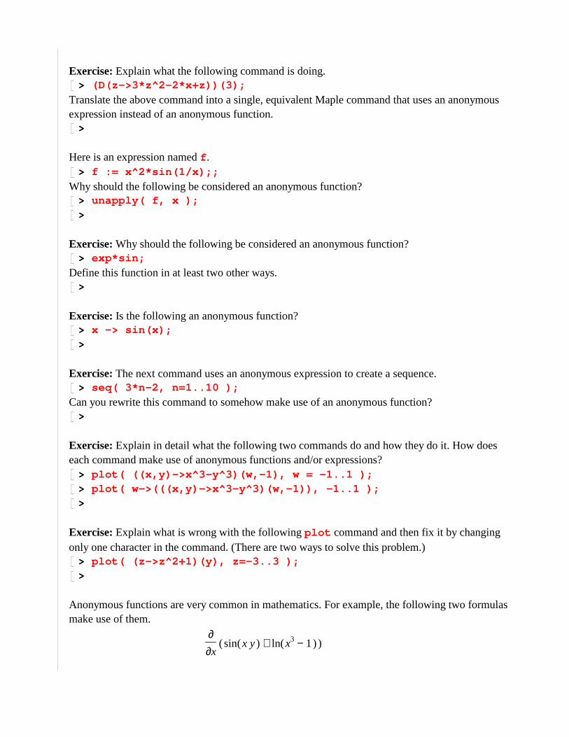
Exercise: Explain what the following command is doing.> (D(z->3*z^2-2*x+z))(3);

Translate the above command into a single, equivalent Maple command that uses an anonymous expression instead of an anonymous function.

>

Here is an expression named f .> f := x^2*sin(1/x);;

Why should the following be considered an anonymous function?> unapply( f, x );>

Exercise: Why should the following be considered an anonymous function?> exp*sin;

Define this function in at least two other ways.>

Exercise: Is the following an anonymous function?> x -> sin(x);>

Exercise: The next command uses an anonymous expression to create a sequence.> seq( 3*n-2, n=1..10 );

Can you rewrite this command to somehow make use of an anonymous function?>

Exercise: Explain in detail what the following two commands do and how they do it. How does each command make use of anonymous functions and/or expressions?

> plot( ((x,y)->x^3-y^3)(w,-1), w = -1..1 );> plot( w->(((x,y)->x^3-y^3)(w,-1)), -1..1 );>

Exercise: Explain what is wrong with the following plot command and then fix it by changing only one character in the command. (There are two ways to solve this problem.)

> plot( (z->z^2+1)(y), z=-3..3 );>

Anonymous functions are very common in mathematics. For example, the following two formulas make use of them.

∂∂x

( ) + ( )sin x y ( )ln − x3 1

d�

� − + 16 x5 20 x3 5 x x

Mathematics textbooks are filled with formulas like these. We usually do not think of such formulas as using "anonymous functions". The concept of an anonymous function is not all that useful in most mathematics books. But as we will see, in Maple, and in computer programming in general, the concept of an anonymous function is very useful.

>

>

4.12. Functions that return a function (optional)It is possible to do some unusual things with the definitions of Maple functions. For example, we can define functions whose return value is another function. Here is a simple example.

> f := a -> ( y->a*y );

The Maple function f takes in a number and returns a function that multiplies its input by the number.

> f(3);

So f(3) is a function that multiplies its input by 3. Here is how we apply f(3) to the input 4.> f(3)(4);

Here is another call to f .> f(-5);

Here is a call to the function returned by f .> f(-5)(2);

In some sense you can think of f as a function of two variables. > f(x)(y);

But this can be misleading. Consider the next two function calls.> f(x);> f(y);>

Exercise: Consider the output of f(y) .> f(y);

Now explain why the following function call does not return 9.> f(y)(3);>

Here is an example of how we might use the idea of a function that returns a function. Start with a function of two variables.

> f := (x,y) -> 3*x^2+5*y^2;

Now we shall define "slicing" functions for f . If we hold one input to f fixed, then we get a new function of a single variable that is sometimes called a "slice" (or a "section") of f . If we just plug a constant into f for say y , then we get back an expression in x .

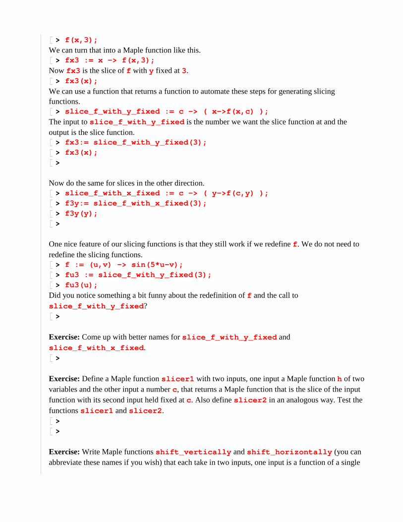
> f(x,3);

We can turn that into a Maple function like this.> fx3 := x -> f(x,3);

Now fx3 is the slice of f with y fixed at 3.> fx3(x);

We can use a function that returns a function to automate these steps for generating slicing functions.

> slice_f_with_y_fixed := c -> ( x->f(x,c) );

The input to slice_f_with_y_fixed is the number we want the slice function at and the output is the slice function.

> fx3:= slice_f_with_y_fixed(3);> fx3(x);>

Now do the same for slices in the other direction.> slice_f_with_x_fixed := c -> ( y->f(c,y) );> f3y:= slice_f_with_x_fixed(3);> f3y(y);>

One nice feature of our slicing functions is that they still work if we redefine f . We do not need to redefine the slicing functions.

> f := (u,v) -> sin(5*u-v);> fu3 := slice_f_with_y_fixed(3);> fu3(u);

Did you notice something a bit funny about the redefinition of f and the call to slice_f_with_y_fixed ?

>

Exercise: Come up with better names for slice_f_with_y_fixed and slice_f_with_x_fixed .

>

Exercise: Define a Maple function slicer1 with two inputs, one input a Maple function h of two variables and the other input a number c , that returns a Maple function that is the slice of the input function with its second input held fixed at c . Also define slicer2 in an analogous way. Test the functions slicer1 and slicer2 .

> >

Exercise: Write Maple functions shift_vertically and shift_horizontally (you can abbreviate these names if you wish) that each take in two inputs, one input is a function of a single

variable and the other input is a number, and that each return a function. The procedure shift_vertically produces an output function that is its input function shifted vertically by the amount of the input number, and shift_horizontally produces an output function that is its input function shifted horizontally by the amount of the input number. Apply your procedures to some test functions and show that they work by graphing the test functions and their shifted versions in the same graph.

>

Exercise: Suppose you wanted to write a version of slicer1 that worked on expressions instead of Maple functions. That is, suppose you wanted to write a procedure slicer1 that takes as its input an expression of two variables and a number, and produces as its output an expression in one variable that represents the slice function of the function represented by the input expression with one of the inputs held fixed at the input number. What kind of problems are you going to have with trying to write this version of slicer1 ? (The problems you will have are in fact one of the major weaknesses of working with expressions.)

>

The idea of a function that returns a function is very common in mathematics. Sometimes these kinds of functions are given the special name functionals. One important branch of mathematics is called functional analysis. It is the study of the properties of functionals. In particular, functional analysis tries to generalize classical analysis, that is calculus with real and vector valued functions, to function valued functions.

Functions that return functions are also important in computer science. They lead to an important family of programming languages called functional programming languages. The two most common functional programming languages are called Lisp and Scheme. These languages are very different from more traditional programming languages like C, C++, Java, Fortran and Basic. As might be expected, functional programming languages have a much more mathematical feel to them then the more traditional programming languages. Functional programming languages have played an important role in the development of the field of artificial intelligence.

When we get to the worksheets about Maple programming, we will generalize the idea of a function that returns a function to the idea of a procedure that returns a procedure.

>

>

4.13. More examples of expressions vs. Maple functions (optional)These examples are meant to show that there are still a lot of subtle things to learn about variables and functions and how Maple handles them. Do not expect to fully understand these examples now. You should return to these examples after you have gone through the worksheet on Maple's

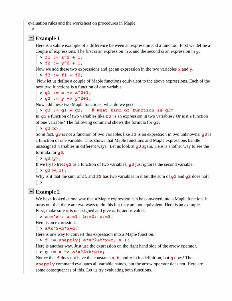
evaluation rules and the worksheet on procedures in Maple.>

Example 1Here is a subtle example of a difference between an expression and a function. First we define a couple of expressions. The first is an expression in x and the second is an expression in y .

> f1 := x^2 + 1;> f2 := y^2 + 1;

Now we add these two expressions and get an expression in the two variables x and y .> f3 := f1 + f2;

Now let us define a couple of Maple functions equivalent to the above expressions. Each of the next two functions is a function of one variable.

> g1 := x -> x^2+1;> g2 := y -> y^2+1;

Now add these two Maple functions; what do we get?> g3 := g1 + g2; # What kind of function is g3?

Is g3 a function of two variables like f3 is an expression in two variables? Or is it a function of one variable? The following command shows the formula for g3 .

> g3(x);

So in fact, g3 is not a function of two variables like f3 is an expression in two unknowns; g3 is a function of one variable. This shows that Maple functions and Maple expressions handle unassigned variables in different ways. Let us look at g3 again. Here is another way to see the formula for g3 .

> g3(y);

If we try to treat g3 as a function of two variables, g3 just ignores the second variable.> g3(w,z);

Why is it that the sum of f1 and f2 has two variables in it but the sum of g1 and g2 does not?>

Example 2We have looked at one way that a Maple expression can be converted into a Maple function. It turns out that there are two ways to do this but they are not equivalent. Here is an example. First, make sure x is unassigned and give a, b, and c values.

> x:='x': a:=1: b:=2: c:=3:

Here is an expression.> a*x^2+b*x+c;

Here is one way to convert this expression into a Maple function.> f := unapply( a*x^2+b*x+c, x );

Here is another way. Just use the expression on the right hand side of the arrow operator.> g := x -> a*x^2+b*x+c;

Notice that f does not have the constants a, b, and c in its definition, but g does! The unapply command evaluates all variable names, but the arrow operator does not. Here are some consequences of this. Let us try evaluating both functions.

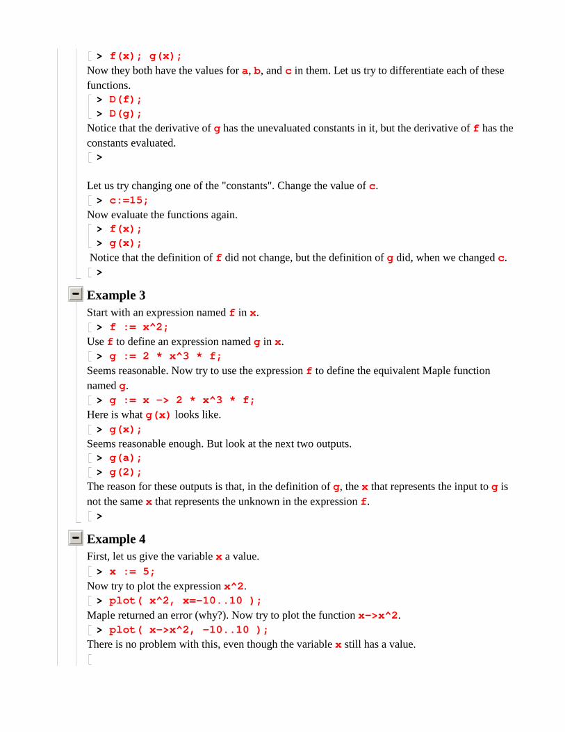
> f(x); g(x);

Now they both have the values for a, b, and c in them. Let us try to differentiate each of these functions.

> D(f);> D(g);

Notice that the derivative of g has the unevaluated constants in it, but the derivative of f has the constants evaluated.

>

Let us try changing one of the "constants". Change the value of c .> c:=15;

Now evaluate the functions again.> f(x);> g(x);

Notice that the definition of f did not change, but the definition of g did, when we changed c .>

Example 3Start with an expression named f in x .

> f := x^2;

Use f to define an expression named g in x .> g := 2 * x^3 * f;

Seems reasonable. Now try to use the expression f to define the equivalent Maple function named g.

> g := x -> 2 * x^3 * f;

Here is what g(x) looks like.> g(x);

Seems reasonable enough. But look at the next two outputs.> g(a);> g(2);

The reason for these outputs is that, in the definition of g, the x that represents the input to g is not the same x that represents the unknown in the expression f .

>

Example 4First, let us give the variable x a value.

> x := 5;

Now try to plot the expression x^2 .> plot( x^2, x=-10..10 );

Maple returned an error (why?). Now try to plot the function x->x^2 .> plot( x->x^2, -10..10 );

There is no problem with this, even though the variable x still has a value.

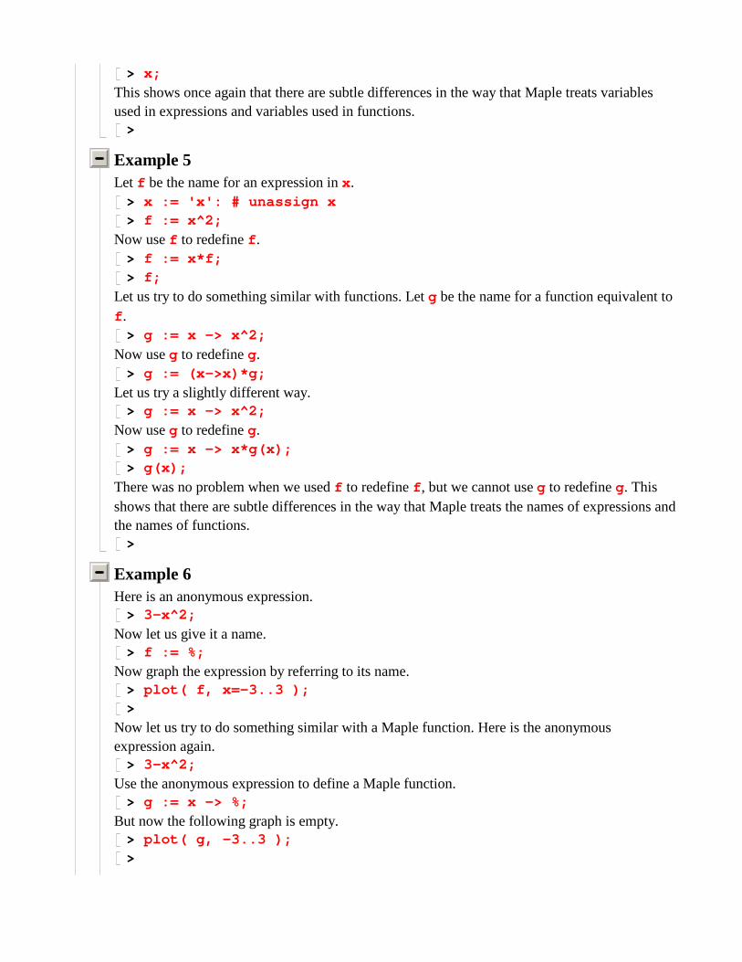
> x;

This shows once again that there are subtle differences in the way that Maple treats variables used in expressions and variables used in functions.

>

Example 5Let f be the name for an expression in x .

> x := 'x': # unassign x> f := x^2;

Now use f to redefine f .> f := x*f;> f;

Let us try to do something similar with functions. Let g be the name for a function equivalent to f .

> g := x -> x^2;

Now use g to redefine g.> g := (x->x)*g;

Let us try a slightly different way.> g := x -> x^2;

Now use g to redefine g.> g := x -> x*g(x);> g(x);

There was no problem when we used f to redefine f , but we cannot use g to redefine g. This shows that there are subtle differences in the way that Maple treats the names of expressions and the names of functions.

>

Example 6Here is an anonymous expression.

> 3-x^2;

Now let us give it a name.> f := %;

Now graph the expression by referring to its name.> plot( f, x=-3..3 );>

Now let us try to do something similar with a Maple function. Here is the anonymous expression again.

> 3-x^2;

Use the anonymous expression to define a Maple function.> g := x -> %;

But now the following graph is empty.> plot( g, -3..3 );>

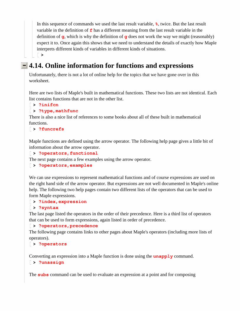
In this sequence of commands we used the last result variable, %, twice. But the last result variable in the definition of f has a different meaning from the last result variable in the definition of g, which is why the definition of g does not work the way we might (reasonably) expect it to. Once again this shows that we need to understand the details of exactly how Maple interprets different kinds of variables in different kinds of situations.

>

4.14. Online information for functions and expressionsUnfortunately, there is not a lot of online help for the topics that we have gone over in this worksheet.

Here are two lists of Maple's built in mathematical functions. These two lists are not identical. Each list contains functions that are not in the other list.

> ?inifcn> ?type,mathfunc

There is also a nice list of references to some books about all of these built in mathematical functions.

> ?funcrefs

Maple functions are defined using the arrow operator. The following help page gives a little bit of information about the arrow operator.

> ?operators,functional

The next page contains a few examples using the arrow operator.> ?operators,examples

We can use expressions to represent mathematical functions and of course expressions are used on the right hand side of the arrow operator. But expressions are not well documented in Maple's online help. The following two help pages contain two different lists of the operators that can be used to form Maple expressions.

> ?index,expression> ?syntax

The last page listed the operators in the order of their precedence. Here is a third list of operators that can be used to form expressions, again listed in order of precedence.

> ?operators,precedence

The following page contains links to other pages about Maple's operators (including more lists of operators).

> ?operators

Converting an expression into a Maple function is done using the unapply command.> ?unassign

The subs command can be used to evaluate an expression at a point and for composing

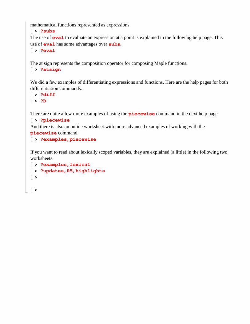
mathematical functions represented as expressions.> ?subs

The use of eval to evaluate an expression at a point is explained in the following help page. This use of eval has some advantages over subs .

> ?eval

The at sign represents the composition operator for composing Maple functions.> ?atsign

We did a few examples of differentiating expressions and functions. Here are the help pages for both differentiation commands.

> ?diff> ?D

There are quite a few more examples of using the piecewise command in the next help page.> ?piecewise

And there is also an online worksheet with more advanced examples of working with the piecewise command.

> ?examples,piecewise

If you want to read about lexically scoped variables, they are explained (a little) in the following two worksheets.

> ?examples,lexical> ?updates,R5,highlights>

>