Maple for Math Majors

Roger Kraft

Department of Mathematics, Computer Science, and Statistics

Purdue University Calumet

roger@calumet.purdue.edu

7. Mathematical Identities and Maple's Assume Facility

7.1. IntroductionIn this worksheet we consider mathematical identities. We show that identities are another way to use an equalsign in mathematical notation. We show how to get Maple to demonstrate a number of mathematical identities.We look at the case of identities that are true for only some values of the variables in the identity. This leads usto introduce Maple's assuming command and Maple's assume facility, which allow us to place assumptions on the values that an unassigned variable is supposed to represent.

>

7.2. Mathematical identitiesIn Worksheet 2 we emphasized that equal signs are used in mathematical formulas in at least two different ways, to represent an assignment and as part of an equation. For example, we interpret the equal sign in the formula x = 0 as an assignment and we assume that the formula means that x is a name for zero. We translate this into Maple as the assignment statement x:=0. On the other hand we interpret the formula x 2 - 2 x - 1 = 0 as an equation that can be solved for x. We translate this directly into Maple as the equation x^2-2*x-1=0, which can then be solved using the solve command.

> x^2-2*x-1=0;

> solve( %, x );

Now consider the formula 1 - x( )2 = 1 - 2 x + x 2. Here the equal sign is definitely not an assignment. And thisis not really an equation either since this formula is not asking for which x is the equation true. The equation istrue for all x and in fact the purpose of the formula is to tell us that. This formula is an example of an identity and the purpose of the equal sign in an identity is to tell us that the left and right hand sides are (under certain circumstances) interchangeable. So now we have a third use for an equal sign in a mathematical formula. Howshould this use of an equal sign be translated into Maple? We would want Maple to tell us that 1 - 2 x + x 2 is equivalent to 1 - x( )2. The expand command in Maple will tell us exactly that.

> expand( (1-x)^2 );

So the mathematical identity 1 - x( )2 = 1 - 2 x + x 2 is represented in Maple by an application of Maple's

expand command. If we take this identity and turn it around, 1 - 2 x + x 2 = 1 - x( )2, then we can get Maple

to demonstrate this identity by applying Maple's factor command.

> factor( 1-2*x+x^2 );

Mathematics has a huge number of identities and Maple has quite a few commands that can be used to demonstrate identities. Let us look at a number of examples of different kinds of identities and how Maple candemonstrate them.

The factor command allows Maple to demonstrate the following algebraic identity.3 x 2 - 7 x - 20 = x - 4( ) 3 x + 5( )

> factor( 3*x^2-7*x-20 );

Here is an identity involving the exponential function.

e x e y = e x + y( )

For this identity we can use the simplify command.

> simplify( exp(x)*exp(y) );

Here is a trig identity.

sin x( ) cos y( ) = sin x + y( )2

+ sin x - y( )2

For this identity we need the combine command.

> combine( sin(x)*cos(y) );

Here is an identity about a rational function.a - b

x - a( ) x - b( ) = 1x - a

- 1x - b

For this identity we need the convert command with the option parfrac.

> convert( (a-b)/((x-a)*(x-b)), parfrac, x );

The option parfrac is an abbreviation of "partial fraction". So this convert command converts a rational function into its partial fraction expansion.

>

Here is an identity involving the integers.

Sk = 1

n

k = n n + 1( )

2

We translate this into an application of Maple's sum command.

> sum( k, k=1..n );

Well, we are not quite there yet. Try the factor command.

> factor( % );

We can combine these two steps into one Maple command.

> factor( sum(k, k=1..n) );

Suppose we want Maple to actually display the whole identity in its output, not just the right hand side of the identity. We can do this by using what is called the inert form of Maple's sum command. Many Maple commands have an inert form, which is the command with its initial letter capitalized. The inert form of sum isSum. The inert form of a Maple command (if the command has an inert form) does not carry out the action of command. Instead, the inert form is a way to tell Maple to typeset the command in Standard Math Notation as the command's output. So for example, the inert form of sum does not do any summation, but it does display a nicely typeset summation formula.

> Sum( k, k=1..n );

(The fact that the summation symbol is black, instead of blue, is meant to show that it is the result of an inert command.) So here is how we get Maple to display both sides of our identity. Use the inert form of sum on the left hand side of an equal sign and the regular sum on the right hand side.

> Sum(k, k=1..n) = factor( sum(k, k=1..n) );

Here is an integral identity, displayed by using both the inert and the regular forms of the int command.

> Int( sqrt(x^2+a^2), x ) = int( sqrt(x^2+a^2), x );

We can get Maple to display both sides of our previous identities. These identities do not need the use of an inert command.

> (1-x)^2 = expand( (1-x)^2 );

> 3*x^2-7*x-20 = factor( 3*x^2-7*x-20 );

> exp(x)*exp(y) = simplify( exp(x)*exp(y) );

> sin(x)*cos(y) = combine( sin(x)*cos(y) );

> (a-b)/((x-a)*(x-b)) = convert( (a-b)/((x-a)*(x-b)), parfrac, x );

>

Here is how we would do each of these identities in its other direction.

> 1-2*x+x^2 = factor( 1-2*x+x^2 );

> (3*x+5)*(x-4) = expand( (3*x+5)*(x-4) );

> exp(x+y) = expand( exp(x+y) );

> sin(x+y)/2 + sin(x-y)/2 = expand( sin(x+y)/2 + sin(x-y)/2 );

> 1/(x-a) - 1/(x-b) = simplify( 1/(x-a) - 1/(x-b) );

>

Notice that it takes quite a few Maple commands to demonstrate these identities and it is not always obvious which Maple command might be useful for demonstrating a particular identity. In the next worksheet we will go over some of the details of using these commands and we will try to give some guidelines on which command should be used when. In particular, the commands that are covered in detail in the next worksheet are simplify, factor, expand, combine, and convert.

All of the identities demonstrated above have the property that they are true for all the possible values of the variables in the identity. Not all identities have this property. For some identities, the identity is true for only some values of the variables involved. For example, the trigonometric identity arcsin sin x( )( ) = x is true only if x is between -π/2 and π/2. Because of this, Maple will not readily demonstrate this identity for us.

> arcsin( sin(x) );

> simplify( % );

But we can tell the simplify command to make an assumption about the possible values that the variable x can represent.

> simplify( %% ) assuming RealRange(-Pi/2, Pi/2);

In the next section we look at more examples of identities that are true for only some values of the variables involved. And in the two sections after that we show how to make use of Maple's assuming and assume commands to place assumptions on what values a variable can represent.

>

>

7.3. A closer look at mathematical identitiesAn important idea to remember about mathematical identities is that they need not be true for all values of the variables involved. An identity may be true only when the variables in the identity have their values restricted to a certain set of numbers. To put it another way, an identity may be true only if we make an assumption about what values the variables in the identity may represent. For example, here are three identities, each with a set of numbers for which the identity is true.

x 2 = x is true for all positive real numbers,

x 2 = x| | is true for all real numbers,

x 2 = csgn x( ) x is true for all complex numbers.

Let us see how we get Maple to demonstrate each of these identities.

>

Maple assumes, by default, that variables represent complex numbers. So Maple will, by default, only expressidentities that are true for all complex numbers. Of the three identities from the previous paragraph, the last

one is true for all complex numbers, and so that is how Maple will, by default, simplify the expression sqrt(x^2).

> sqrt(x^2);

> simplify( % );

On the other hand, if we tell the simplify command to make an assumption about x, then it will simplify the expression sqrt(x^2) differently. Here is how we use the assuming command with simplify to express the first of the three identities.

> simplify( sqrt(x^2) ) assuming positive;

Here is how we use the assuming command with simplify to express the second of the three identities.

> simplify( sqrt(x^2) ) assuming real;

>

The following three commands demonstrate the last three identities in equation form.

> sqrt(x^2) = (simplify( sqrt(x^2) ) assuming positive);

> sqrt(x^2) = (simplify( sqrt(x^2) ) assuming real);

> sqrt(x^2) = simplify( sqrt(x^2) );

Notice how, in each output, there is no indication of the assumption that is being used in the identity. To see the assumption being used (or to even know that an assumption was made), you must look at the command that produced the identity.

>

When we write an identity in equation form and then solve the equation, we should find that the equation is true for every possible value of the variable in the identity. Let us try using the solve command with the above identities.

> sqrt(x^2) = simplify( sqrt(x^2) );

> solve( %, {x} );

That is not what we expected. Let us try one of the other identities.

> sqrt(x^2) = (simplify( sqrt(x^2) ) assuming positive);

> solve( %, {x} );

This result says that the equation is true for every value of x (that is what we should have gotten for the previous equation). But this identity is true only with the assumption that x is a positive real number and there is nothing in the result from solve that implies that x must be a positive real number. These last two examples show that solve need not work very well with equations that express identities.

It is important to remember that Maple will almost always by default assume that a variable in an expression represents a complex number. Maple does not know about any of the common conventions used in mathematics books for variables. For example, the variable n is almost always used in mathematics books to

represent an integer, as in sin n π( ) = 0. But in the following expression, Maple considers n to be an arbitrary complex number and it will not simplify sin(n*Pi) to 0.

> sin(n*Pi);

> simplify( % );

But if we explicitly tell simplify to assume that n is an integer, then we get the simplification that we expect.

> simplify( sin(n*Pi) ) assuming integer;

Similarly, to get the simplification cos n π( ) = -1( )n we need to explicitly tell simplify to assume that n is an integer.

> cos(n*Pi);

> simplify( % ) assuming integer;

And of course, -1( )n is either 1 or -1, depending on whether n is even or odd.

> simplify( % ) assuming even;

> simplify( %% ) assuming odd;

Here are two more identities that depend on even and odd integers.

> cos(n*Pi/2);

> simplify( % ) assuming even;

> sin(n*Pi/2);

> simplify( % ) assuming odd;

>

Exercise: Make sure that you understand why the last result is correct. Maple's way of expressing the last result is not how it would be done in a calculus book. What is another way to express the simplification of sin n π

2æçè

ö÷ø

when n represents an odd integer?

>

For a variety of reasons, using identities in Maple can sometimes be a bit tricky. For one thing, under Maple's assumption that variables represent complex numbers, some identities that are very familiar to us from algebra and calculus are no longer true. For example, here is a very common identity used in calculus,

e x( )y = e x y( )

.

This identity is not true for all complex numbers. Here is a simple counterexample. First evaluate the

expression e x( )y with x = I 2 π and y = 1

2.

> eval( exp(x)^y, {x=I*2*Pi, y=1/2} );

Now evaluate the expression ex y( )

with x = I 2 π and y = 12

. We get a different result.

> eval( exp(x*y), {x=I*2*Pi, y=1/2} );

The identity that we want can be demonstrated by the simplify command, but only if we place certain assumptions on the variables.

> exp(x)^y;

> simplify( % ); # with no assumptions on the variables

The last command shows that without any assumptions, simplify will not demonstrate the identity. But if we make the standard assumption from calculus courses, that variables represent real numbers, then we can get simplify to demonstrate the identity.

> simplify( %% ) assuming real;

This example shows that even for very simple, common identities from calculus, we may need to do something non obvious, like make an assumption, in order to be able to make use of the identity in Maple.

>

Here is an example that shows another way in which using identities in Maple can be tricky. In a course on complex variables, it can be shown that the following two identities are true.

e x( )y = e x y( )

is true if y is an integer (and x is any complex number)

e x( )y = e x y( )is true if x is a real number (and y is any complex number)

Using the combine and assuming commands, we can demonstrate the first of these two identities.

> exp(x)^y;

> combine( % ) assuming y::integer;

(Notice that we used a form of the assuming command that placed an assumption on only one of the two variables in the identity.) But combine and assuming will not demonstrate the second of the two identities.

> exp(x)^y;

> combine( % ) assuming x::real;

But now consider the following example. Instead of working with e x( )y, let us try working with b x( )

y with

the assumption that b is a positive real number (and of course, e is one of the positive real numbers).

> (b^x)^y;

> combine( % ) assuming b::positive, x::real;

So combine and assuming were able to demonstrate the more general identity with any positive b, but theycould not demonstrate the more specific identity with b = e. What this shows is that Maple's abilities to work with assumptions are not foolproof. Sometimes Maple refuses to make use of a certain identity and we need toapproach the identity from a different point of view.

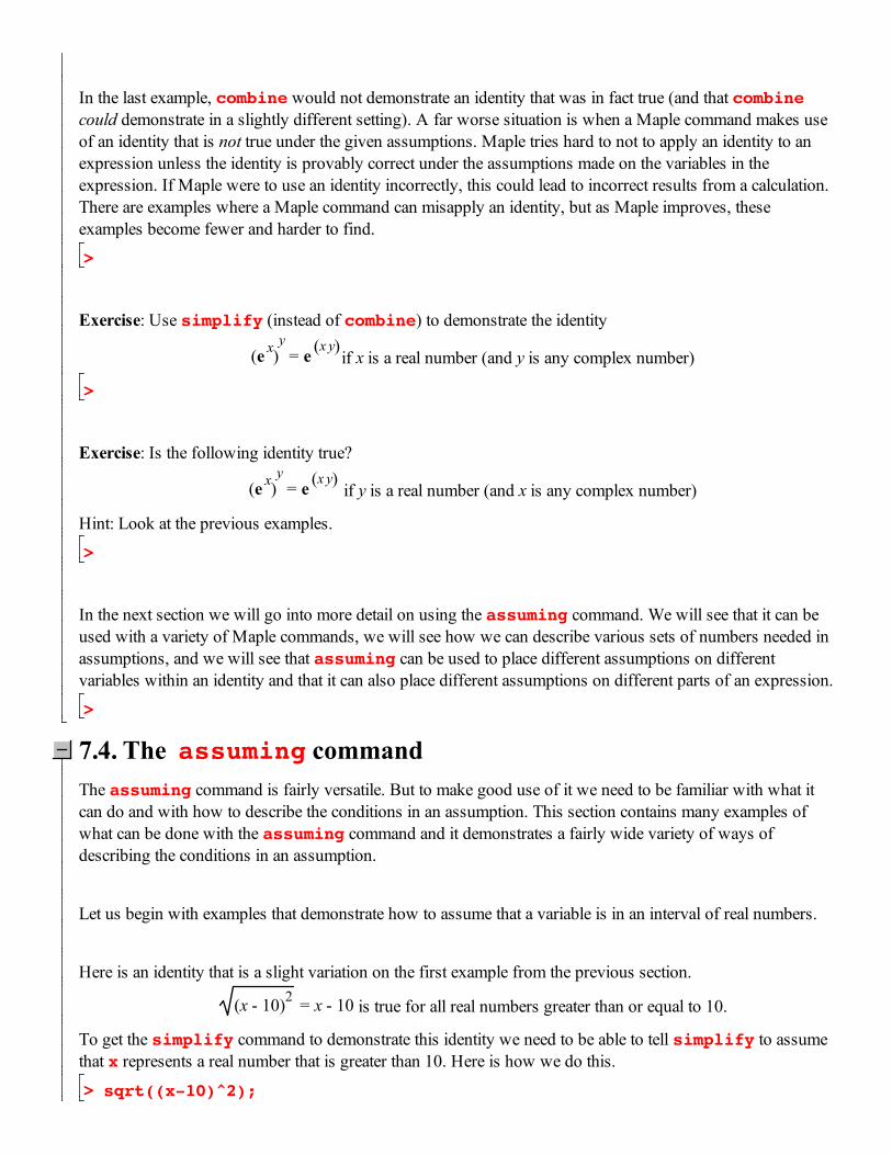
In the last example, combine would not demonstrate an identity that was in fact true (and that combine could demonstrate in a slightly different setting). A far worse situation is when a Maple command makes use of an identity that is not true under the given assumptions. Maple tries hard to not to apply an identity to an expression unless the identity is provably correct under the assumptions made on the variables in the expression. If Maple were to use an identity incorrectly, this could lead to incorrect results from a calculation. There are examples where a Maple command can misapply an identity, but as Maple improves, these examples become fewer and harder to find.

>

Exercise: Use simplify (instead of combine) to demonstrate the identity

e x( )y = e x y( )

if x is a real number (and y is any complex number)

>

Exercise: Is the following identity true?

e x( )y = e x y( )

if y is a real number (and x is any complex number)

Hint: Look at the previous examples.

>

In the next section we will go into more detail on using the assuming command. We will see that it can be used with a variety of Maple commands, we will see how we can describe various sets of numbers needed in assumptions, and we will see that assuming can be used to place different assumptions on different variables within an identity and that it can also place different assumptions on different parts of an expression.

>

7.4. The assuming commandThe assuming command is fairly versatile. But to make good use of it we need to be familiar with what it can do and with how to describe the conditions in an assumption. This section contains many examples of what can be done with the assuming command and it demonstrates a fairly wide variety of ways of describing the conditions in an assumption.

Let us begin with examples that demonstrate how to assume that a variable is in an interval of real numbers.

Here is an identity that is a slight variation on the first example from the previous section.

x - 10( )2 = x - 10 is true for all real numbers greater than or equal to 10.

To get the simplify command to demonstrate this identity we need to be able to tell simplify to assume that x represents a real number that is greater than 10. Here is how we do this.

> sqrt((x-10)^2);

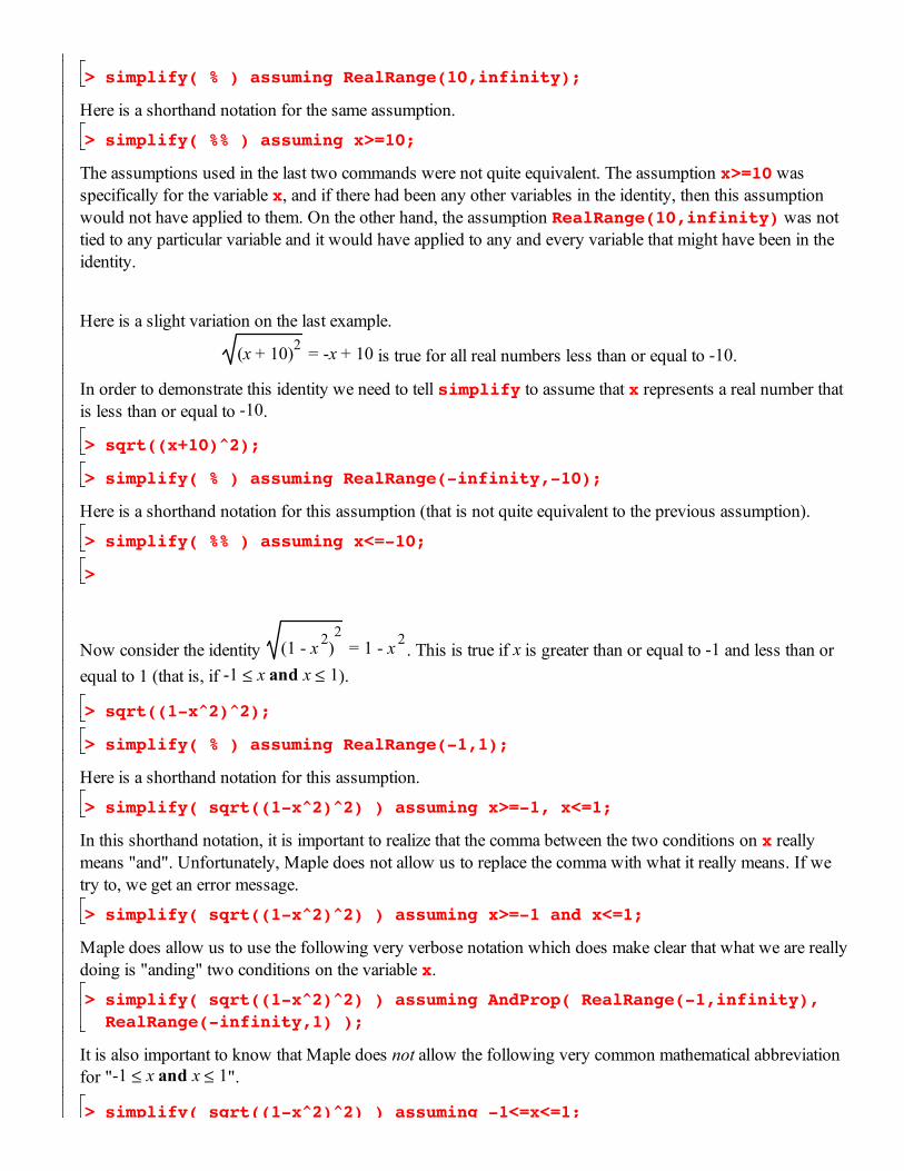
> simplify( % ) assuming RealRange(10,infinity);

Here is a shorthand notation for the same assumption.

> simplify( %% ) assuming x>=10;

The assumptions used in the last two commands were not quite equivalent. The assumption x>=10 was specifically for the variable x, and if there had been any other variables in the identity, then this assumption would not have applied to them. On the other hand, the assumption RealRange(10,infinity) was not tied to any particular variable and it would have applied to any and every variable that might have been in the identity.

Here is a slight variation on the last example.

x + 10( )2 = -x + 10 is true for all real numbers less than or equal to -10.

In order to demonstrate this identity we need to tell simplify to assume that x represents a real number that is less than or equal to -10.

> sqrt((x+10)^2);

> simplify( % ) assuming RealRange(-infinity,-10);

Here is a shorthand notation for this assumption (that is not quite equivalent to the previous assumption).

> simplify( %% ) assuming x<=-10;

>

Now consider the identity 1 - x 2( )2

= 1 - x 2. This is true if x is greater than or equal to -1 and less than or

equal to 1 (that is, if -1 £ x and x £ 1).

> sqrt((1-x^2)^2);

> simplify( % ) assuming RealRange(-1,1);

Here is a shorthand notation for this assumption.

> simplify( sqrt((1-x^2)^2) ) assuming x>=-1, x<=1;

In this shorthand notation, it is important to realize that the comma between the two conditions on x really means "and". Unfortunately, Maple does not allow us to replace the comma with what it really means. If we try to, we get an error message.

> simplify( sqrt((1-x^2)^2) ) assuming x>=-1 and x<=1;

Maple does allow us to use the following very verbose notation which does make clear that what we are reallydoing is "anding" two conditions on the variable x.

> simplify( sqrt((1-x^2)^2) ) assuming AndProp( RealRange(-1,infinity), RealRange(-infinity,1) );

It is also important to know that Maple does not allow the following very common mathematical abbreviation for "-1 £ x and x £ 1".

> simplify( sqrt((1-x^2)^2) ) assuming -1<=x<=1;

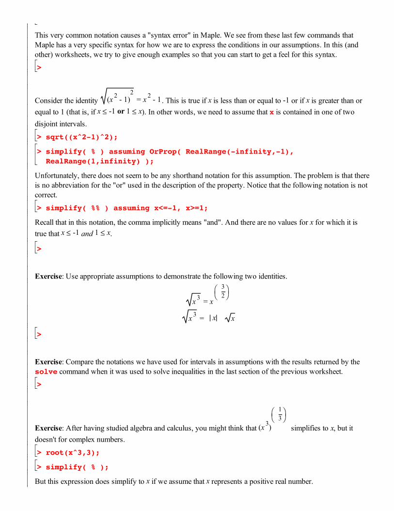
This very common notation causes a "syntax error" in Maple. We see from these last few commands that Maple has a very specific syntax for how we are to express the conditions in our assumptions. In this (and other) worksheets, we try to give enough examples so that you can start to get a feel for this syntax.

>

Consider the identity x 2 - 1( )2

= x 2 - 1. This is true if x is less than or equal to -1 or if x is greater than or equal to 1 (that is, if x £ -1 or 1 £ x). In other words, we need to assume that x is contained in one of two disjoint intervals.

> sqrt((x^2-1)^2);

> simplify( % ) assuming OrProp( RealRange(-infinity,-1), RealRange(1,infinity) );

Unfortunately, there does not seem to be any shorthand notation for this assumption. The problem is that thereis no abbreviation for the "or" used in the description of the property. Notice that the following notation is not correct.

> simplify( %% ) assuming x<=-1, x>=1;

Recall that in this notation, the comma implicitly means "and". And there are no values for x for which it is true that x £ -1 and 1 £ x.

>

Exercise: Use appropriate assumptions to demonstrate the following two identities.

x 3 = x

32

æè

öø

x 3 = x| | x

>

Exercise: Compare the notations we have used for intervals in assumptions with the results returned by the solve command when it was used to solve inequalities in the last section of the previous worksheet.

>

Exercise: After having studied algebra and calculus, you might think that x 3( )

13

æè

öø

simplifies to x, but it doesn't for complex numbers.

> root(x^3,3);

> simplify( % );

But this expression does simplify to x if we assume that x represents a positive real number.

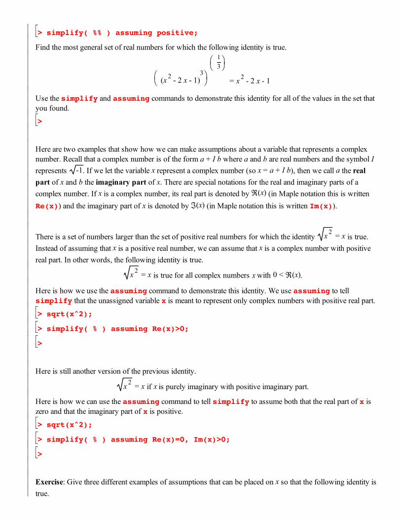
> simplify( %% ) assuming positive;

Find the most general set of real numbers for which the following identity is true.

x 2 - 2 x - 1( )3æ

èöø

13

æè

öø

= x 2 - 2 x - 1

Use the simplify and assuming commands to demonstrate this identity for all of the values in the set that you found.

>

Here are two examples that show how we can make assumptions about a variable that represents a complex number. Recall that a complex number is of the form a + I b where a and b are real numbers and the symbol I represents -1. If we let the variable x represent a complex number (so x = a + I b), then we call a the real part of x and b the imaginary part of x. There are special notations for the real and imaginary parts of a complex number. If x is a complex number, its real part is denoted by  x( ) (in Maple notation this is written Re(x)) and the imaginary part of x is denoted by Á x( ) (in Maple notation this is written Im(x)).

There is a set of numbers larger than the set of positive real numbers for which the identity x 2 = x is true. Instead of assuming that x is a positive real number, we can assume that x is a complex number with positive real part. In other words, the following identity is true.

x 2 = x is true for all complex numbers x with 0 < Â x( ).

Here is how we use the assuming command to demonstrate this identity. We use assuming to tell simplify that the unassigned variable x is meant to represent only complex numbers with positive real part.

> sqrt(x^2);

> simplify( % ) assuming Re(x)>0;

>

Here is still another version of the previous identity.

x 2 = x if x is purely imaginary with positive imaginary part.

Here is how we can use the assuming command to tell simplify to assume both that the real part of x is zero and that the imaginary part of x is positive.

> sqrt(x^2);

> simplify( % ) assuming Re(x)=0, Im(x)>0;

>

Exercise: Give three different examples of assumptions that can be placed on x so that the following identity istrue.

x 2 = -x

Demonstrate your assumptions using simplify and assuming.

>

So far in this section we have looked at some specific ways to describe assumptions about the values that a variable can represent. In particular, we have seen how to assume that a variable represents numbers from intervals of real numbers, and we have seen how to make some simple assumptions about complex numbers. Now let us turn to some general facts about assumptions and the assuming command.

Assumptions made with assuming do not apply just to specific commands like simplify or combine. Assumptions can apply to any expression. For example, the following command tells Maple to evaluate the expression sqrt(x^2) under the assumption that the variable is positive.

> sqrt(x^2) assuming positive;

Notice that the assumption caused Maple to automatically simplify the expression. The assumption had an effect on the expression even without there being an explicit simplify command. This shows that assumptions apply to expressions and not just to Maple commands.

The last example brings up a bit of a confusing topic. It is not always clear when Maple's automatic simplification rules take affect. For example, as we just saw, the following command leads to an automatic simplification.

> sqrt(x^2) assuming positive;

But the following very similar command does not lead to an automatic simplification.

> sqrt(x^2) assuming real;

In this case, to get the simplification implied by the assumption, we must apply the simplify command along with the assumption.

> simplify( sqrt(x^2) ) assuming real;

It is important to realize that in the command

> sqrt(x^2) assuming real;

the assumption really does apply to the expression. Maple does not ignore the assumption. But the assumptiondoes not, in this command, trigger an automatic simplification like it does when the assumption is that the variable is positive. As I stated above, it is not always clear what will or will not trigger Maple's automatic simplification rules.

A corollary of the fact that assumptions apply to expressions is the fact that an assuming command can be placed inside of an expression and by using parentheses its effect can be limited to a piece of the expression. In the next example, only one occurrence of x in the following expression has an assumption placed on it.

> (sqrt(x^2) assuming positive) + sqrt(x^2);

>

An assumption made with the assuming command can either be tied to a specific variable in an expression or it can apply to all of the variables in the expression. In the following command, the assumption applies to both variables in the expression being simplified.

> sqrt((y-3)^2) + sqrt(x^2);

> simplify( % ) assuming RealRange(3, infinity);

But in the next command, the assumption is specific to just the variable y.

> simplify( %% ) assuming y::RealRange(3, infinity);

Here is another way to express the assumption for y only.

> simplify( %%% ) assuming y>=3;

The following command puts different assumptions on x and y.

> simplify( sqrt((y-3)^2) + sqrt(x^2) ) assuming y>=3, x::negative;

>

Exercise: Are the following two commands equivalent?

> (sqrt(x^2) assuming positive) + sqrt(y^2);

> sqrt(x^2) + sqrt(y^2) assuming x::positive;

Are the following two commands equivalent?

> (y+sqrt(x^2) assuming positive) + sqrt(y^2);

> y+sqrt(x^2) + sqrt(y^2) assuming x::positive;

>

The assuming command can be used with many different Maple commands. Here are a number of examplesthat show what can be done when assuming is combined with some other Maple commands.

Let us start with a few well know identities from calculus that are not true for complex numbers so we need touse assumptions to get Maple to demonstrate the identities. The logarithmic identities

ln x y( ) = ln x( ) + ln y( )

ln x y( ) = y ln x( )

are not true for all complex numbers. However, if we use an assumption, then we can demonstrate these identities using the expand command.

> expand( ln(x*y) );

> expand( ln(x*y) ) assuming positive;

> expand( ln(x^y) );

> expand( ln(x^y) ) assuming positive;

We can also do the opposite direction of the first identity by using combine along with asssuming.

> combine( ln(x)+ln(y) );

> combine( ln(x)+ln(y) ) assuming positive;

>

The following logarithmic identity is not true for arbitrary complex numbers.ln e x( ) = x

But it is true for all real numbers, and Maple will automatically simplify it if we assume the x is a real number.

> ln(exp(x));

> ln(exp(x)) assuming real;

>

The identity x n y n = x y( )n is not true for all complex numbers. In fact, it is not even true for all real numbers (let x and y both be -1 and let n be one half). But it is true for all complex numbers x and y if we assume that n is an integer.

> simplify( x^n*y^n ) assuming n::integer;

The identity is also true if we assume that x, y, and n are all positive real numbers, but simplify will not demonstrate the identity with this assumption.

> simplify( x^n*y^n ) assuming positive;

>

The frac and trunc commands compute the fractional part and integer part of a real number. The fractional part of any integer is 0 and frac returns the correct answer when we assume that its input is an integer.

> frac( x ) assuming integer;

The integer part of an integer is the integer itself and trunc returns the correct answer when we assume that its input is an integer.

> trunc( x ) assuming integer;

Just because a command can understand some assumptions does not mean that it can understand any assumption. For example, the following two commands should return x and 0 respectively (why?), but they do not.

> frac( x ) assuming RealRange(0,Open(1));

> trunc( x ) assuming RealRange(0,Open(1));

>

Here is an example of an integral that has an unassigned parameter in it (notice that this is the inert form of the integral command).

> Int( exp(a*x), x=0..infinity );

Here is what Maple does with this integral without knowing anything specific about the value of the parametera.

> int( exp(a*x), x=0..infinity );

Let us redo the integral using various assumptions about the parameter a.

> int( exp(a*x), x=0..infinity ) assuming a<0;

> int( exp(a*x), x=0..infinity ) assuming a>0;

>

Exercise: What is not quite right about Maple's result for the following command?

> int( exp(a*x), x=0..infinity ) assuming a<=0;

>

There are many other kinds of identities and many different kinds of sets of numbers that an identity can be true for besides the ones demonstrated in this section. But the assuming command is not versatile enough tohandle all of them. In the next section we will look at Maple's assume command, which is more versatile andcan be used in more situations than the assuming command.

>

>

7.5. Using Maple's assume facilityEarlier in this worksheet we used the assuming command to demonstrate the following identity.

x 2 = x is true for all positive real numbers.

We can also use Maple's assume command to demonstrate this identity. The assume command allows us to"permanently" attach an assumption to a variable. We can use assume to tell Maple that the unassigned variable x is meant to represent only real, positive numbers.

> assume( x, positive );

The assume command did not return anything. But we can use the about command to find out that Maple is now making an assumption about the values represented by x.

> about( x );

Many Maple commands can make use of this information about the values that x is supposed to represent. In fact, Maple itself will make use of this information and automatically simplify the expression sqrt(x^2) and thereby demonstrate the identity that we want.

> sqrt(x^2);

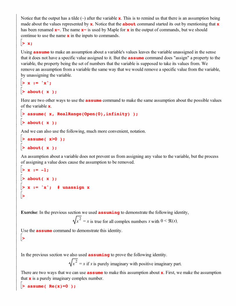
Notice that the output has a tilde (~) after the variable x. This is to remind us that there is an assumption being made about the values represented by x. Notice that the about command started its out by mentioning that x has been renamed x~. The name x~ is used by Maple for x in the output of commands, but we should continue to use the name x in the inputs to commands.

> x;

Using assume to make an assumption about a variable's values leaves the variable unassigned in the sense that it does not have a specific value assigned to it. But the assume command does "assign" a property to the variable, the property being the set of numbers that the variable is supposed to take its values from. We remove an assumption from a variable the same way that we would remove a specific value from the variable, by unassigning the variable.

> x := 'x';

> about( x );

Here are two other ways to use the assume command to make the same assumption about the possible valuesof the variable x.

> assume( x, RealRange(Open(0),infinity) );

> about( x );

And we can also use the following, much more convenient, notation.

> assume( x>0 );

> about( x );

An assumption about a variable does not prevent us from assigning any value to the variable, but the process of assigning a value does cause the assumption to be removed.

> x := -1;

> about( x );

> x := 'x'; # unassign x

>

Exercise: In the previous section we used assuming to demonstrate the following identity,

x 2 = x is true for all complex numbers x with 0 < Â x( ).

Use the assume command to demonstrate this identity.

>

In the previous section we also used assuming to prove the following identity.

x 2 = x if x is purely imaginary with positive imaginary part.

There are two ways that we can use assume to make this assumption about x. First, we make the assumptionthat x is a purely imaginary complex number.

> assume( Re(x)=0 );

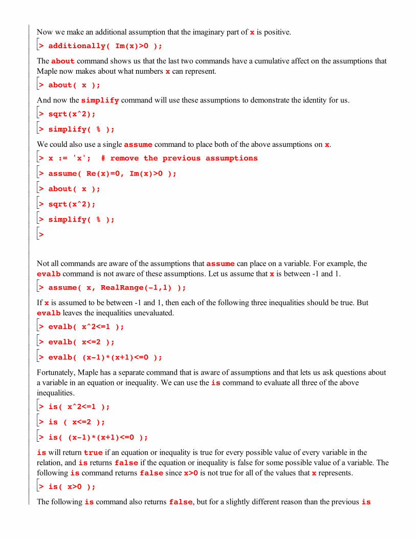
Now we make an additional assumption that the imaginary part of x is positive.

> additionally( Im(x)>0 );

The about command shows us that the last two commands have a cumulative affect on the assumptions that Maple now makes about what numbers x can represent.

> about( x );

And now the simplify command will use these assumptions to demonstrate the identity for us.

> sqrt(x^2);

> simplify( % );

We could also use a single assume command to place both of the above assumptions on x.

> x := 'x'; # remove the previous assumptions

> assume( Re(x)=0, Im(x)>0 );

> about( x );

> sqrt(x^2);

> simplify( % );

>

Not all commands are aware of the assumptions that assume can place on a variable. For example, the evalb command is not aware of these assumptions. Let us assume that x is between -1 and 1.

> assume( x, RealRange(-1,1) );

If x is assumed to be between -1 and 1, then each of the following three inequalities should be true. But evalb leaves the inequalities unevaluated.

> evalb( x^2<=1 );

> evalb( x<=2 );

> evalb( (x-1)*(x+1)<=0 );

Fortunately, Maple has a separate command that is aware of assumptions and that lets us ask questions about a variable in an equation or inequality. We can use the is command to evaluate all three of the above inequalities.

> is( x^2<=1 );

> is ( x<=2 );

> is( (x-1)*(x+1)<=0 );

is will return true if an equation or inequality is true for every possible value of every variable in the relation, and is returns false if the equation or inequality is false for some possible value of a variable. The following is command returns false since x>0 is not true for all of the values that x represents.

> is( x>0 );

The following is command also returns false, but for a slightly different reason than the previous is

command.

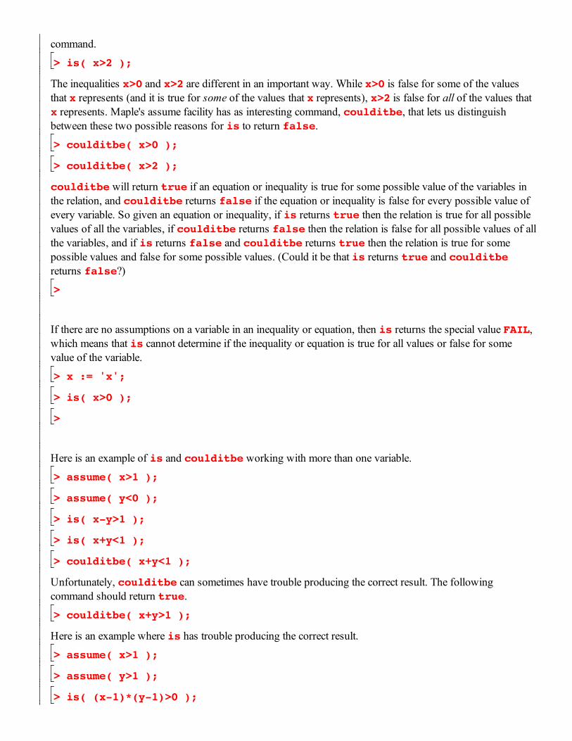
> is( x>2 );

The inequalities x>0 and x>2 are different in an important way. While x>0 is false for some of the values that x represents (and it is true for some of the values that x represents), x>2 is false for all of the values that x represents. Maple's assume facility has as interesting command, coulditbe, that lets us distinguish between these two possible reasons for is to return false.

> coulditbe( x>0 );

> coulditbe( x>2 );

coulditbe will return true if an equation or inequality is true for some possible value of the variables in the relation, and coulditbe returns false if the equation or inequality is false for every possible value of every variable. So given an equation or inequality, if is returns true then the relation is true for all possible values of all the variables, if coulditbe returns false then the relation is false for all possible values of allthe variables, and if is returns false and coulditbe returns true then the relation is true for some possible values and false for some possible values. (Could it be that is returns true and coulditbe returns false?)

>

If there are no assumptions on a variable in an inequality or equation, then is returns the special value FAIL, which means that is cannot determine if the inequality or equation is true for all values or false for some value of the variable.

> x := 'x';

> is( x>0 );

>

Here is an example of is and coulditbe working with more than one variable.

> assume( x>1 );

> assume( y<0 );

> is( x-y>1 );

> is( x+y<1 );

> coulditbe( x+y<1 );

Unfortunately, coulditbe can sometimes have trouble producing the correct result. The following command should return true.

> coulditbe( x+y>1 );

Here is an example where is has trouble producing the correct result.

> assume( x>1 );

> assume( y>1 );

> is( (x-1)*(y-1)>0 );

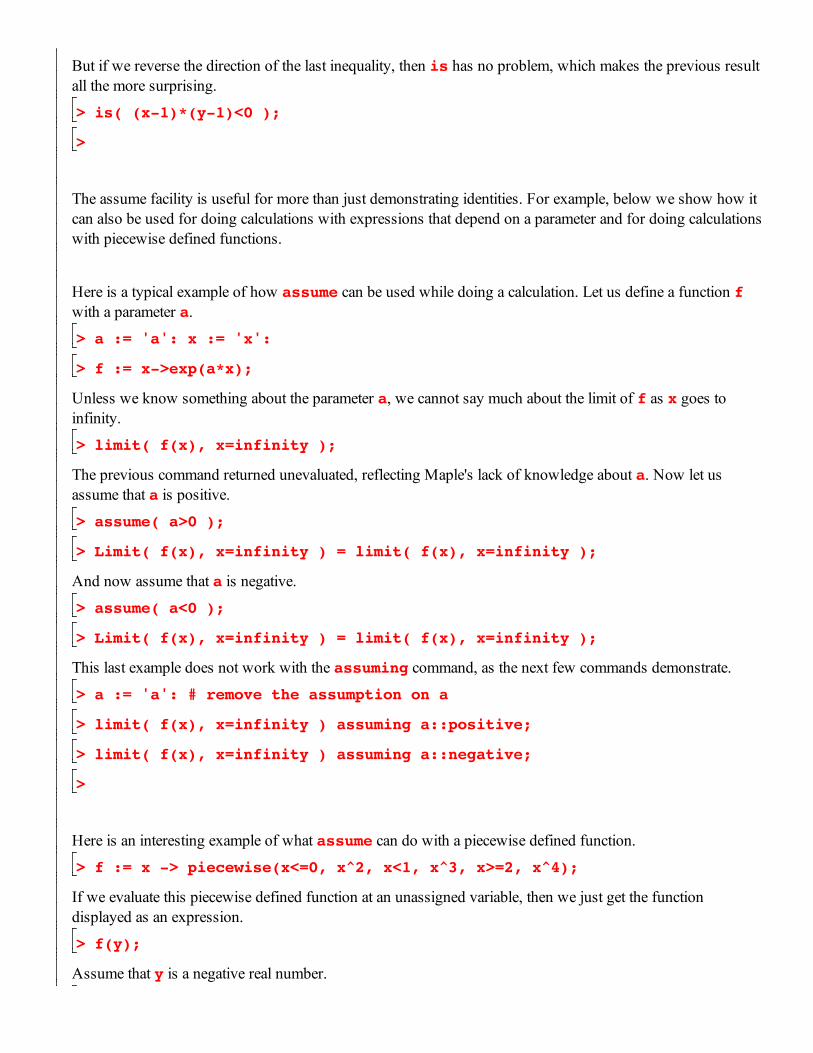
But if we reverse the direction of the last inequality, then is has no problem, which makes the previous result all the more surprising.

> is( (x-1)*(y-1)<0 );

>

The assume facility is useful for more than just demonstrating identities. For example, below we show how it can also be used for doing calculations with expressions that depend on a parameter and for doing calculationswith piecewise defined functions.

Here is a typical example of how assume can be used while doing a calculation. Let us define a function f with a parameter a.

> a := 'a': x := 'x':

> f := x->exp(a*x);

Unless we know something about the parameter a, we cannot say much about the limit of f as x goes to infinity.

> limit( f(x), x=infinity );

The previous command returned unevaluated, reflecting Maple's lack of knowledge about a. Now let us assume that a is positive.

> assume( a>0 );

> Limit( f(x), x=infinity ) = limit( f(x), x=infinity );

And now assume that a is negative.

> assume( a<0 );

> Limit( f(x), x=infinity ) = limit( f(x), x=infinity );

This last example does not work with the assuming command, as the next few commands demonstrate.

> a := 'a': # remove the assumption on a

> limit( f(x), x=infinity ) assuming a::positive;

> limit( f(x), x=infinity ) assuming a::negative;

>

Here is an interesting example of what assume can do with a piecewise defined function.

> f := x -> piecewise(x<=0, x^2, x<1, x^3, x>=2, x^4);

If we evaluate this piecewise defined function at an unassigned variable, then we just get the function displayed as an expression.

> f(y);

Assume that y is a negative real number.

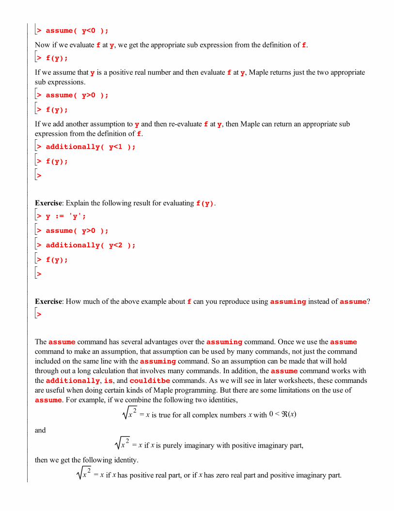
> assume( y<0 );

Now if we evaluate f at y, we get the appropriate sub expression from the definition of f.

> f(y);

If we assume that y is a positive real number and then evaluate f at y, Maple returns just the two appropriate sub expressions.

> assume( y>0 );

> f(y);

If we add another assumption to y and then re-evaluate f at y, then Maple can return an appropriate sub expression from the definition of f.

> additionally( y<1 );

> f(y);

>

Exercise: Explain the following result for evaluating f(y).

> y := 'y';

> assume( y>0 );

> additionally( y<2 );

> f(y);

>

Exercise: How much of the above example about f can you reproduce using assuming instead of assume?

>

The assume command has several advantages over the assuming command. Once we use the assume command to make an assumption, that assumption can be used by many commands, not just the command included on the same line with the assuming command. So an assumption can be made that will hold through out a long calculation that involves many commands. In addition, the assume command works with the additionally, is, and coulditbe commands. As we will see in later worksheets, these commands are useful when doing certain kinds of Maple programming. But there are some limitations on the use of assume. For example, if we combine the following two identities,

x 2 = x is true for all complex numbers x with 0 < Â x( )

and

x 2 = x if x is purely imaginary with positive imaginary part,

then we get the following identity.

x 2 = x if x has positive real part, or if x has zero real part and positive imaginary part.

I do not know of any easy way to use the assume command to make the assumptions needed to demonstrate this identity.

>

>

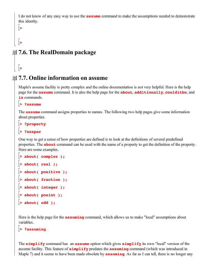
7.6. The RealDomain package

>

7.7. Online information on assumeMaple's assume facility is pretty complex and the online documentation is not very helpful. Here is the help page for the assume command. It is also the help page for the about, additionally, coulditbe, and is commands.

> ?assume

The assume command assigns properties to names. The following two help pages give some information about properties.

> ?property

> ?asspar

One way to get a sense of how properties are defined is to look at the definitions of several predefined properties. The about command can be used with the name of a property to get the definition of the property.Here are some examples.

> about( complex );

> about( real );

> about( positive );

> about( fraction );

> about( integer );

> about( posint );

> about( odd );

Here is the help page for the assuming command, which allows us to make "local" assumptions about variables.

> ?assuming

The simplify command has an assume option which gives simplify its own "local" version of the assume facility. This feature of simplify predates the assuming command (which was introduced in Maple 7) and it seems to have been made obsolete by assuming. As far as I can tell, there is no longer any

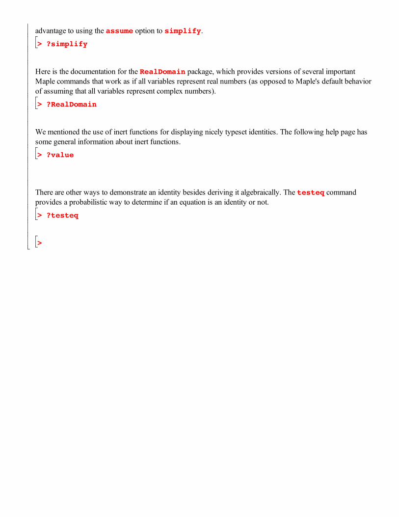
advantage to using the assume option to simplify.

> ?simplify

Here is the documentation for the RealDomain package, which provides versions of several important Maple commands that work as if all variables represent real numbers (as opposed to Maple's default behavior of assuming that all variables represent complex numbers).

> ?RealDomain

We mentioned the use of inert functions for displaying nicely typeset identities. The following help page has some general information about inert functions.

> ?value

There are other ways to demonstrate an identity besides deriving it algebraically. The testeq command provides a probabilistic way to determine if an equation is an identity or not.

> ?testeq

>