Embed Size (px)
Citation preview
Maple 9Learning Guide
Based in part on the work of B. W. Char
c© Maplesoft, a division of Waterloo Maple Inc. 2003
ii •
Maplesoft, Maple, Maple Application Center, Maple Student Center,and Maplet are all trademarks of Waterloo Maple Inc.
c© Maplesoft, a division of Waterloo Maple Inc. 2003. All rights re-served.
The electronic version (PDF) of this book may be downloaded andprinted for personal use or stored as a copy on a personal machine. Theelectronic version (PDF) of this book may not be distributed. Informationin this document is subject to change without notice and does not repre-sent a commitment on the part of the vendor. The software described inthis document is furnished under a license agreement and may be used orcopied only in accordance with the agreement. It is against the law to copysoftware on any medium except as specifically allowed in the agreement.
Windows is a registered trademark of Microsoft Corporation.Java and all Java based marks are trademarks or registered trade-
marks of Sun Microsystems, Inc. in the United States and other countries.Maplesoft is independent of Sun Microsystems, Inc.
All other trademarks are the property of their respective owners.
This document was produced using a special version of Maple thatreads and updates LATEX files.
Printed in Canada
ISBN 1-894511-42-5
Contents
Preface 1Audience . . . . . . . . . . . . . . . . . . . . . . . . . . . . . . 1Manual Set . . . . . . . . . . . . . . . . . . . . . . . . . . . . . 1Conventions . . . . . . . . . . . . . . . . . . . . . . . . . . . . . 2Customer Feedback . . . . . . . . . . . . . . . . . . . . . . . . . 2
1 Introduction to Maple 3Worksheet Graphical Interface . . . . . . . . . . . . . . . 3Modes . . . . . . . . . . . . . . . . . . . . . . . . . . . . . 3
2 Mathematics with Maple: The Basics 5In This Chapter . . . . . . . . . . . . . . . . . . . . . . . 5Maple Help System . . . . . . . . . . . . . . . . . . . . . . 5
2.1 Introduction . . . . . . . . . . . . . . . . . . . . . . . . . . 5Exact Expressions . . . . . . . . . . . . . . . . . . . . . . 6
2.2 Numerical Computations . . . . . . . . . . . . . . . . . . 7Integer Computations . . . . . . . . . . . . . . . . . . . . 7Commands for Working With Integers . . . . . . . . . . . 9Exact Arithmetic—Rationals, Irrationals, and Constants . 10Floating-Point Approximations . . . . . . . . . . . . . . . 12Arithmetic with Special Numbers . . . . . . . . . . . . . . 14Mathematical Functions . . . . . . . . . . . . . . . . . . . 15
2.3 Basic Symbolic Computations . . . . . . . . . . . . . . . . 162.4 Assigning Expressions to Names . . . . . . . . . . . . . . 18
Syntax for Naming an Object . . . . . . . . . . . . . . . . 18Guidelines for Maple Names . . . . . . . . . . . . . . . . . 19Maple Arrow Notation in Defining Functions . . . . . . . 19The Assignment Operator . . . . . . . . . . . . . . . . . . 20Predefined and Reserved Names . . . . . . . . . . . . . . . 20
2.5 Basic Types of Maple Objects . . . . . . . . . . . . . . . . 21
iii
iv • Contents
Expression Sequences . . . . . . . . . . . . . . . . . . . . 21Lists . . . . . . . . . . . . . . . . . . . . . . . . . . . . . . 23Sets . . . . . . . . . . . . . . . . . . . . . . . . . . . . . . 24Operations on Sets and Lists . . . . . . . . . . . . . . . . 25Arrays . . . . . . . . . . . . . . . . . . . . . . . . . . . . . 27Tables . . . . . . . . . . . . . . . . . . . . . . . . . . . . . 31Strings . . . . . . . . . . . . . . . . . . . . . . . . . . . . . 32
2.6 Expression Manipulation . . . . . . . . . . . . . . . . . . . 33The simplify Command . . . . . . . . . . . . . . . . . . 33The factor Command . . . . . . . . . . . . . . . . . . . . 34The expand Command . . . . . . . . . . . . . . . . . . . . 35The convert Command . . . . . . . . . . . . . . . . . . . 36The normal Command . . . . . . . . . . . . . . . . . . . . 36The combine Command . . . . . . . . . . . . . . . . . . . 37The map Command . . . . . . . . . . . . . . . . . . . . . . 38The lhs and rhs Commands . . . . . . . . . . . . . . . . 39The numer and denom Commands . . . . . . . . . . . . . . 39The nops and op Commands . . . . . . . . . . . . . . . . 40Common Questions about Expression Manipulation . . . 41
2.7 Conclusion . . . . . . . . . . . . . . . . . . . . . . . . . . 42
3 Finding Solutions 43In This Chapter . . . . . . . . . . . . . . . . . . . . . . . 43
3.1 The Maple solve Command . . . . . . . . . . . . . . . . 43Examples Using the solve Command . . . . . . . . . . . 43Verifying Solutions . . . . . . . . . . . . . . . . . . . . . . 45Restricting Solutions . . . . . . . . . . . . . . . . . . . . . 47Exploring Solutions . . . . . . . . . . . . . . . . . . . . . . 48The unapply Command . . . . . . . . . . . . . . . . . . . 49The assign Command . . . . . . . . . . . . . . . . . . . . 51The RootOf Command . . . . . . . . . . . . . . . . . . . . 53
3.2 Solving Numerically Using the fsolve Command . . . . . 54Limitations on solve . . . . . . . . . . . . . . . . . . . . . 55
3.3 Other Solvers . . . . . . . . . . . . . . . . . . . . . . . . . 58Finding Integer Solutions . . . . . . . . . . . . . . . . . . 58Finding Solutions Modulo m . . . . . . . . . . . . . . . . 58Solving Recurrence Relations . . . . . . . . . . . . . . . . 59
3.4 Polynomials . . . . . . . . . . . . . . . . . . . . . . . . . . 59Sorting and Collecting . . . . . . . . . . . . . . . . . . . . 60Mathematical Operations . . . . . . . . . . . . . . . . . . 61Coefficients and Degrees . . . . . . . . . . . . . . . . . . . 62
Contents • v
Root Finding and Factorization . . . . . . . . . . . . . . . 633.5 Calculus . . . . . . . . . . . . . . . . . . . . . . . . . . . . 653.6 Solving Differential Equations Using the dsolve Command 713.7 Conclusion . . . . . . . . . . . . . . . . . . . . . . . . . . 77
4 Maple Organization 79In This Chapter . . . . . . . . . . . . . . . . . . . . . . . 79
4.1 The Organization of Maple . . . . . . . . . . . . . . . . . 79The Maple Library . . . . . . . . . . . . . . . . . . . . . . 80
4.2 The Maple Packages . . . . . . . . . . . . . . . . . . . . . 82List of Packages . . . . . . . . . . . . . . . . . . . . . . . . 82Example Packages . . . . . . . . . . . . . . . . . . . . . . 87The Student Package . . . . . . . . . . . . . . . . . . . . . 87Worksheet Examples . . . . . . . . . . . . . . . . . . . . . 88The LinearAlgebra Package . . . . . . . . . . . . . . . . . 94The Matlab Package . . . . . . . . . . . . . . . . . . . . . 96The Statistics Package . . . . . . . . . . . . . . . . . . . . 98The simplex Linear Optimization Package . . . . . . . . 101
4.3 Conclusion . . . . . . . . . . . . . . . . . . . . . . . . . . 102
5 Plotting 103In This Chapter . . . . . . . . . . . . . . . . . . . . . . . 103Plotting Commands in Main Maple Library . . . . . . . . 103Plotting Commands in Packages . . . . . . . . . . . . . . 103Publishing Material with Plots . . . . . . . . . . . . . . . 104
5.1 Graphing in Two Dimensions . . . . . . . . . . . . . . . . 104Parametric Plots . . . . . . . . . . . . . . . . . . . . . . . 106Polar Coordinates . . . . . . . . . . . . . . . . . . . . . . 108Functions with Discontinuities . . . . . . . . . . . . . . . . 111Functions with Singularities . . . . . . . . . . . . . . . . . 112Multiple Functions . . . . . . . . . . . . . . . . . . . . . . 114Plotting Data Points . . . . . . . . . . . . . . . . . . . . . 116Refining Plots . . . . . . . . . . . . . . . . . . . . . . . . . 118
5.2 Graphing in Three Dimensions . . . . . . . . . . . . . . . 119Parametric Plots . . . . . . . . . . . . . . . . . . . . . . . 121Spherical Coordinates . . . . . . . . . . . . . . . . . . . . 121Cylindrical Coordinates . . . . . . . . . . . . . . . . . . . 124Refining Plots . . . . . . . . . . . . . . . . . . . . . . . . . 125Shading and Lighting Schemes . . . . . . . . . . . . . . . 126
5.3 Animation . . . . . . . . . . . . . . . . . . . . . . . . . . . 127Animation in Two Dimensions . . . . . . . . . . . . . . . 128
vi • Contents
Animation in Three Dimensions . . . . . . . . . . . . . . . 1305.4 Annotating Plots . . . . . . . . . . . . . . . . . . . . . . . 132
Labeling a Plot . . . . . . . . . . . . . . . . . . . . . . . . 1335.5 Composite Plots . . . . . . . . . . . . . . . . . . . . . . . 134
Placing Text in Plots . . . . . . . . . . . . . . . . . . . . . 1365.6 Special Types of Plots . . . . . . . . . . . . . . . . . . . . 137
Visualization Component of the Student Package . . . . . 1435.7 Manipulating Graphical Objects . . . . . . . . . . . . . . 144
Using the display Command . . . . . . . . . . . . . . . . 1445.8 Code for Color Plates . . . . . . . . . . . . . . . . . . . . 1495.9 Interactive Plot Builder . . . . . . . . . . . . . . . . . . . 1525.10 Conclusion . . . . . . . . . . . . . . . . . . . . . . . . . . 153
6 Evaluation and Simplification 155Working with Expressions in Maple . . . . . . . . . . . . . 155In This Chapter . . . . . . . . . . . . . . . . . . . . . . . 155
6.1 Mathematical Manipulations . . . . . . . . . . . . . . . . 156Expanding Polynomials as Sums . . . . . . . . . . . . . . 156Collecting the Coefficients of Like Powers . . . . . . . . . 158Factoring Polynomials and Rational Functions . . . . . . 161Removing Rational Exponents . . . . . . . . . . . . . . . 163Combining Terms . . . . . . . . . . . . . . . . . . . . . . . 164Factored Normal Form . . . . . . . . . . . . . . . . . . . . 165Simplifying Expressions . . . . . . . . . . . . . . . . . . . 168Simplification with Assumptions . . . . . . . . . . . . . . 169Simplification with Side Relations . . . . . . . . . . . . . . 169Sorting Algebraic Expressions . . . . . . . . . . . . . . . . 171Converting Between Equivalent Forms . . . . . . . . . . . 172
6.2 Assumptions . . . . . . . . . . . . . . . . . . . . . . . . . 174The assume Facility . . . . . . . . . . . . . . . . . . . . . 174The assuming Command . . . . . . . . . . . . . . . . . . 178
6.3 Structural Manipulations . . . . . . . . . . . . . . . . . . 180Mapping a Function onto a List or Set . . . . . . . . . . . 180Choosing Elements from a List or Set . . . . . . . . . . . 182Merging Two Lists . . . . . . . . . . . . . . . . . . . . . . 184Sorting Lists . . . . . . . . . . . . . . . . . . . . . . . . . 185The Parts of an Expression . . . . . . . . . . . . . . . . . 188Substitution . . . . . . . . . . . . . . . . . . . . . . . . . . 196Changing the Type of an Expression . . . . . . . . . . . . 200
6.4 Evaluation Rules . . . . . . . . . . . . . . . . . . . . . . . 202Levels of Evaluation . . . . . . . . . . . . . . . . . . . . . 202
Contents • vii
Last-Name Evaluation . . . . . . . . . . . . . . . . . . . . 203One-Level Evaluation . . . . . . . . . . . . . . . . . . . . 205Commands with Special Evaluation Rules . . . . . . . . . 206Quotation and Unevaluation . . . . . . . . . . . . . . . . . 207Using Quoted Variables as Function Arguments . . . . . . 210Concatenation of Names . . . . . . . . . . . . . . . . . . . 211
6.5 Conclusion . . . . . . . . . . . . . . . . . . . . . . . . . . 213
7 Solving Calculus Problems 215In This Chapter . . . . . . . . . . . . . . . . . . . . . . . 215
7.1 Introductory Calculus . . . . . . . . . . . . . . . . . . . . 215The Derivative . . . . . . . . . . . . . . . . . . . . . . . . 215A Taylor Approximation . . . . . . . . . . . . . . . . . . . 221The Integral . . . . . . . . . . . . . . . . . . . . . . . . . . 232Mixed Partial Derivatives . . . . . . . . . . . . . . . . . . 236
7.2 Ordinary Differential Equations . . . . . . . . . . . . . . . 240The dsolve Command . . . . . . . . . . . . . . . . . . . . 241Example: Taylor Series . . . . . . . . . . . . . . . . . . . . 255When You Cannot Find a Closed Form Solution . . . . . 259Plotting Ordinary Differential Equations . . . . . . . . . . 260Discontinuous Forcing Functions . . . . . . . . . . . . . . 264Interactive ODE Analyzer . . . . . . . . . . . . . . . . . . 269
7.3 Partial Differential Equations . . . . . . . . . . . . . . . . 270The pdsolve Command . . . . . . . . . . . . . . . . . . . 270Changing the Dependent Variable in a PDE . . . . . . . . 272Plotting Partial Differential Equations . . . . . . . . . . . 273
7.4 Conclusion . . . . . . . . . . . . . . . . . . . . . . . . . . 276
8 Input and Output 277In This Chapter . . . . . . . . . . . . . . . . . . . . . . . 277
8.1 Reading Files . . . . . . . . . . . . . . . . . . . . . . . . . 277Reading Columns of Numbers from a File . . . . . . . . . 278Reading Commands from a File . . . . . . . . . . . . . . . 280
8.2 Writing Data to a File . . . . . . . . . . . . . . . . . . . . 281Writing Columns of Numerical Data to a File . . . . . . . 281Saving Expressions in the Maple Internal Format . . . . . 283Converting to LATEX Format . . . . . . . . . . . . . . . . . 284
8.3 Exporting Worksheets . . . . . . . . . . . . . . . . . . . . 286HTML and HTML with MathML . . . . . . . . . . . . . . 286LATEX . . . . . . . . . . . . . . . . . . . . . . . . . . . . . 289Maple Input . . . . . . . . . . . . . . . . . . . . . . . . . . 291
viii • Contents
Maplet Application . . . . . . . . . . . . . . . . . . . . . . 292Maple Text . . . . . . . . . . . . . . . . . . . . . . . . . . 293Plain Text . . . . . . . . . . . . . . . . . . . . . . . . . . . 295RTF . . . . . . . . . . . . . . . . . . . . . . . . . . . . . . 296XML . . . . . . . . . . . . . . . . . . . . . . . . . . . . . . 297
8.4 Printing Graphics . . . . . . . . . . . . . . . . . . . . . . . 298Displaying Graphics in Separate Windows . . . . . . . . . 298Sending Graphics in PostScript Format to a File . . . . . 298Graphics Suitable for HP LaserJet . . . . . . . . . . . . . 299
8.5 Conclusion . . . . . . . . . . . . . . . . . . . . . . . . . . 299
9 Maplet User Interface Customization System 301In This Chapter . . . . . . . . . . . . . . . . . . . . . . . 301
9.1 Example Maplet Application . . . . . . . . . . . . . . . . 3029.2 Terminology . . . . . . . . . . . . . . . . . . . . . . . . . . 3029.3 How to Start the Maplets Package . . . . . . . . . . . . . 3039.4 How to Invoke a Maplet Application from the Maple Work-
sheet . . . . . . . . . . . . . . . . . . . . . . . . . . . . . . 3039.5 How to Close a Maplet Application . . . . . . . . . . . . . 3049.6 How to Work With Maplet Applications and the Maple
Window (Modality) . . . . . . . . . . . . . . . . . . . . . 3049.7 How to Activate a Maplet Application Window . . . . . . 3059.8 How to Terminate and Restart a Maplet Application . . . 3059.9 How to Use Graphical User Interface Shortcuts . . . . . . 305
Drop-down List Boxes . . . . . . . . . . . . . . . . . . . . 305Space Bar and Tab Key . . . . . . . . . . . . . . . . . . 306
9.10 Conclusion . . . . . . . . . . . . . . . . . . . . . . . . . . 3069.11 General Conclusion . . . . . . . . . . . . . . . . . . . . . . 306
Index 307
Preface
This manual introduces important concepts and builds a framework ofknowledge that guides you in your use of the interface and the MapleTM
language. This manual provides an overview of the functionality of Maple.It describes both the symbolic and numeric capabilities, introducing theavailable Maple objects, commands, and methods. Emphasis is placed onfinding solutions, plotting or animating results, and exporting worksheetsto other formats. More importantly, this manual presents the philosophyand methods of use intended by the designers of the system.
Audience
The information in this manual is intended for first time Maple users. Asan adjunct, access to the Maple help system is recommended.
Manual Set
There are three other manuals available for Maple users, the Maple Get-ting Started Guide, the Maple Introductory Programming Guide, andthe Maple Advanced Programming Guide.1
• The Maple Getting Started Guide contains an introduction to thegraphical user interface and a tutorial that outlines using Maple tosolve mathematical problems and create technical documents. It also
1The Student Edition does not include the Maple Introductory Programming Guideand the Maple Advanced Programming Guide. These programming guides can be pur-chased from school and specialty bookstores or directly from Maplesoft.
1
2 • Preface
includes information for new users about the help system, New User’sTour, example worksheets, and the Maplesoft Web site.
• The Maple Introductory Programming Guide introduces the basicMaple programming concepts, such as expressions, data structures,looping and decision mechanisms, procedures, input and output, de-bugging, and the MapletTM User Interface Customization System.
• The Maple Advanced Programming Guide extends the basic Mapleprogramming concepts to more advanced topics, such as modules,input and output, numerical programming, graphics programming,and compiled code.
Whereas this book highlights features of Maple, the help system is acomplete reference manual. There are also examples that you can copy,paste, and execute immediately.
Conventions
This manual uses the following typographical conventions.
• courier font - Maple command, package name, and option name
• bold roman font - dialog, menu, and text field
• italics - new or important concept, option name in a list, and manualtitles
• Note - additional information relevant to the section
• Important - information that must be read and followed
Customer Feedback
Maplesoft welcomes your feedback. For suggestions and comments relatedto this and other manuals, contact [email protected].
1 Introduction to Maple
Maple is a Symbolic Computation System or Computer Algebra Sys-tem. Maple manipulates information in a symbolic or algebraic manner.You can obtain exact analytical solutions to many mathematical prob-lems, including integrals, systems of equations, differential equations,and problems in linear algebra. Maple contains a large set of graphicsroutines for visualizing complicated mathematical information, numeri-cal algorithms for providing estimates and solving problems where exactsolutions do not exist, and a complete and comprehensive programminglanguage for developing custom functions and applications.
Worksheet Graphical InterfaceMaple mathematical functionality is accessed through its advanced worksheet-based graphical interface. A worksheet is a flexible document for exploringmathematical ideas and for creating sophisticated technical reports. Youcan access the power of the Maple computation engine through a varietyof user interfaces: the standard worksheet, the command-line1 version,the classic worksheet (not available on Macintosh r©), and custom-builtMaplet applications. The full Maple system is available through all ofthese interfaces. In this manual, any references to the graphical Mapleinterface refer to the standard worksheet interface. For more informationon the various interface options, refer to the ?versions help page.
ModesYou can use Maple in two modes: as an interactive problem-solving envi-ronment and as a system for generating technical documents.
1The command-line version provides optimum performance. However, the worksheetinterface is easier to use and renders typeset, editable math output and higher qualityplots.
3
4 • Chapter 1: Introduction to Maple
Interactive Problem-Solving Environment Maple allows you to under-take large problems and eliminates your mechanical errors. The interfaceprovides documentation of the steps involved in finding your result. Itallows you to easily modify a step or insert a new one in your solutionmethod. With minimal effort you can compute the new result.
Generating Technical Documents You can create interactive structureddocuments for presentations or publication that contain mathematics inwhich you can change an equation and update the solution automatically.You also can display plots. In addition, you can structure your documentsby using tools such as outlining, styles, and hyperlinks. Outlining allowsyou to collapse sections to hide regions that contain distracting detail.Styles identify keywords, headings, and sections. Hyperlinks allow you tocreate live references that take the reader directly to pages containing re-lated information. The interactive nature of Maple allows you to computeresults and answer questions during presentations. You can clearly andeffectively demonstrate why a seemingly acceptable solution method is in-appropriate, or why a particular modification to a manufacturing processwould lead to loss or profit. Since components of worksheets are directlyassociated with the structure of the document, you can easily translateyour work to other formats, for example, HTML, RTF, and LATEX.
2 Mathematics with Maple:The Basics
This chapter introduces the Maple commands necessary to get youstarted. Use your computer to try the examples as you read.
In This Chapter• Exact calculations
• Numerical computations
• Basic symbolic computations and assignment statements
• Basic types of objects
• Manipulation of objects and the commands
Maple Help SystemAt various points in this guide you are referred to the Maple help system.The help pages provide detailed command and topic information. Youmay choose to access these pages during a Maple session. To use the helpcommand, at the Maple prompt enter a question mark (?) followed bythe name of the command or topic for which you want more information.
?command
2.1 Introduction
This section introduces the following concepts in Maple.
• Semicolon (;) usage
5
6 • Chapter 2: Mathematics with Maple: The Basics
• Representing exact expressions
The most basic computations in Maple are numeric. Maple can func-tion as a conventional calculator with integers or floating-point numbers.Enter the expression using natural syntax. A semicolon (;) marks theend of each calculation. Press enter to perform the calculation.
> 1 + 2;
3
> 1 + 3/2;
5
2
> 2*(3+1/3)/(5/3-4/5);
100
13
> 2.8754/2;
1.437700000
Exact ExpressionsMaple computes exact calculations with rational numbers. Consider asimple example.
> 1 + 1/2;
3
2
The result of 1 + 1/2 is 3/2 not 1.5. To Maple, the rational number3/2 and the floating-point approximation 1.5 are distinct objects. Theability to represent exact expressions allows Maple to preserve moreinformation about their origins and structure. Note that the advantageis greater with more complex expressions. The origin and structure of anumber such as
0.5235987758
2.2 Numerical Computations • 7
are much less clear than for an exact quantity such as
1
6π
Maple can work with rational numbers and arbitrary expressions.It can manipulate integers, floating-point numbers, variables, sets, se-quences, polynomials over a ring, and many more mathematical con-structs. In addition, Maple is also a complete programming language thatcontains procedures, tables, and other programming constructs.
2.2 Numerical Computations
This section introduces the following concepts in Maple.
• Integer computations
• Continuation character (\)
• Ditto operator (%)
• Commands for working with integers
• Exact and floating-point representations of values
• Symbolic representation
• Standard mathematical constants
• Case sensitivity
• Floating-point approximations
• Special numbers
• Mathematical functions
Integer ComputationsInteger calculations are straightforward. Terminate each command witha semicolon.
> 1 + 2;
8 • Chapter 2: Mathematics with Maple: The Basics
3
> 75 - 3;
72
> 5*3;
15
> 120/2;
60
Maple can also work with arbitrarily large integers. The practical limiton integers is approximately 228 digits, depending mainly on the speedand resources of your computer. Maple can calculate large integers, countthe number of digits in a number, and factor integers. For numbers, orother types of continuous output that span more than one line on thescreen, Maple uses the continuation character (\) to indicate that theoutput is continuous. That is, the backslash and following line endingshould be ignored.
> 100!;
933262154439441526816992388562667004907\15968264381621468592963895217599993229\91560894146397615651828625369792082722\37582511852109168640000000000000000000\00000
> length(%);
158
This answer indicates the number of digits in the last example. Theditto operator, (%), is a shorthand reference to the result of the previouscomputation. To recall the second- or third-most previous computationresult, use %% and %%%, respectively.
2.2 Numerical Computations • 9
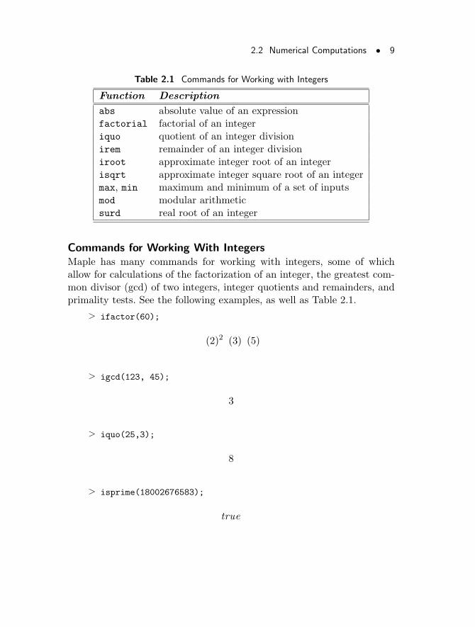
Table 2.1 Commands for Working with Integers
Function Description
abs absolute value of an expressionfactorial factorial of an integeriquo quotient of an integer divisionirem remainder of an integer divisioniroot approximate integer root of an integerisqrt approximate integer square root of an integermax, min maximum and minimum of a set of inputsmod modular arithmeticsurd real root of an integer
Commands for Working With IntegersMaple has many commands for working with integers, some of whichallow for calculations of the factorization of an integer, the greatest com-mon divisor (gcd) of two integers, integer quotients and remainders, andprimality tests. See the following examples, as well as Table 2.1.
> ifactor(60);
(2)2 (3) (5)
> igcd(123, 45);
3
> iquo(25,3);
8
> isprime(18002676583);
true
10 • Chapter 2: Mathematics with Maple: The Basics
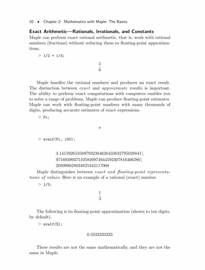
Exact Arithmetic—Rationals, Irrationals, and ConstantsMaple can perform exact rational arithmetic, that is, work with rationalnumbers (fractions) without reducing them to floating-point approxima-tions.
> 1/2 + 1/3;
5
6
Maple handles the rational numbers and produces an exact result.The distinction between exact and approximate results is important.The ability to perform exact computations with computers enables youto solve a range of problems. Maple can produce floating-point estimates.Maple can work with floating-point numbers with many thousands ofdigits, producing accurate estimates of exact expressions.
> Pi;
π
> evalf(Pi, 100);
3.1415926535897932384626433832795028841\97169399375105820974944592307816406286\208998628034825342117068
Maple distinguishes between exact and floating-point representa-tions of values. Here is an example of a rational (exact) number.
> 1/3;
1
3
The following is its floating-point approximation (shown to ten digits,by default).
> evalf(%);
0.3333333333
These results are not the same mathematically, and they are not thesame in Maple.
2.2 Numerical Computations • 11
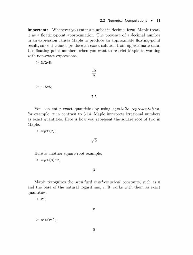
Important: Whenever you enter a number in decimal form, Maple treatsit as a floating-point approximation. The presence of a decimal numberin an expression causes Maple to produce an approximate floating-pointresult, since it cannot produce an exact solution from approximate data.Use floating-point numbers when you want to restrict Maple to workingwith non-exact expressions.
> 3/2*5;
15
2
> 1.5*5;
7.5
You can enter exact quantities by using symbolic representation,for example, π in contrast to 3.14. Maple interprets irrational numbersas exact quantities. Here is how you represent the square root of two inMaple.
> sqrt(2);
√2
Here is another square root example.
> sqrt(3)^2;
3
Maple recognizes the standard mathematical constants, such as πand the base of the natural logarithms, e. It works with them as exactquantities.
> Pi;
π
> sin(Pi);
0
12 • Chapter 2: Mathematics with Maple: The Basics
The exponential function is represented by the Maple function exp.
> exp(1);
e
> ln(exp(5));
5
The example with π may look confusing. When Maple is producingtypeset real-math notation, it attempts to represent mathematical ex-pressions as you might write them yourself. Thus, you enter π as Pi andMaple displays it as π.
Maple is case sensitive. Ensure that you use proper capitalizationwhen stating these constants. The names Pi, pi, and PI are distinct. Thenames pi and PI are used to display the lowercase and uppercase Greekletters π and Π, respectively. For more information on Maple constants,enter ?constants at the Maple prompt.
Floating-Point ApproximationsMaple works with exact values, but it can return a floating-point approxi-mation up to about 228 digits, depending upon your computer’s resources.Ten or twenty accurate digits in floating-point numbers is adequate formany purposes, but two problems severely limit the usefulness of such asystem.
• When subtracting two floating-point numbers of almost equal mag-nitude, the relative error of the difference may be very large. Thisis known as catastrophic cancellation. For example, if two numbersare identical in their first seventeen (of twenty) digits, their differenceis a three-digit number accurate to only three digits. In this case,you would need to use almost forty digits to produce twenty accuratedigits in the answer.
• The mathematical form of the result is more concise, compact, andconvenient than its numerical value. For instance, an exponential func-tion provides more information about the nature of a phenomenonthan a large set of numbers with twenty accurate digits. An exactanalytical description can also determine the behavior of a functionwhen extrapolating to regions for which no data exists.
2.2 Numerical Computations • 13
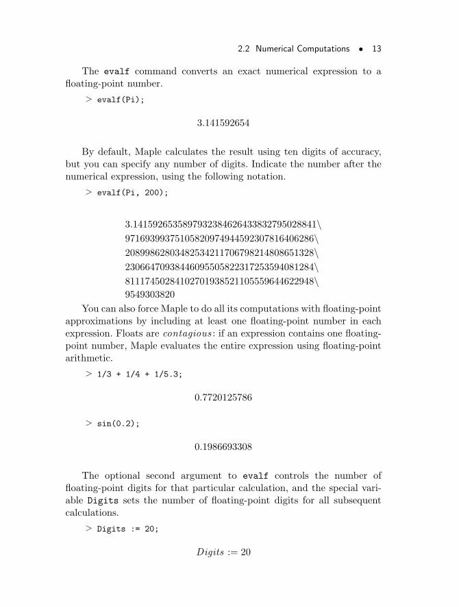
The evalf command converts an exact numerical expression to afloating-point number.
> evalf(Pi);
3.141592654
By default, Maple calculates the result using ten digits of accuracy,but you can specify any number of digits. Indicate the number after thenumerical expression, using the following notation.
> evalf(Pi, 200);
3.1415926535897932384626433832795028841\97169399375105820974944592307816406286\20899862803482534211706798214808651328\23066470938446095505822317253594081284\81117450284102701938521105559644622948\9549303820
You can also force Maple to do all its computations with floating-pointapproximations by including at least one floating-point number in eachexpression. Floats are contagious : if an expression contains one floating-point number, Maple evaluates the entire expression using floating-pointarithmetic.
> 1/3 + 1/4 + 1/5.3;
0.7720125786
> sin(0.2);
0.1986693308
The optional second argument to evalf controls the number offloating-point digits for that particular calculation, and the special vari-able Digits sets the number of floating-point digits for all subsequentcalculations.
> Digits := 20;
Digits := 20
14 • Chapter 2: Mathematics with Maple: The Basics
> sin(0.2);
0.19866933079506121546
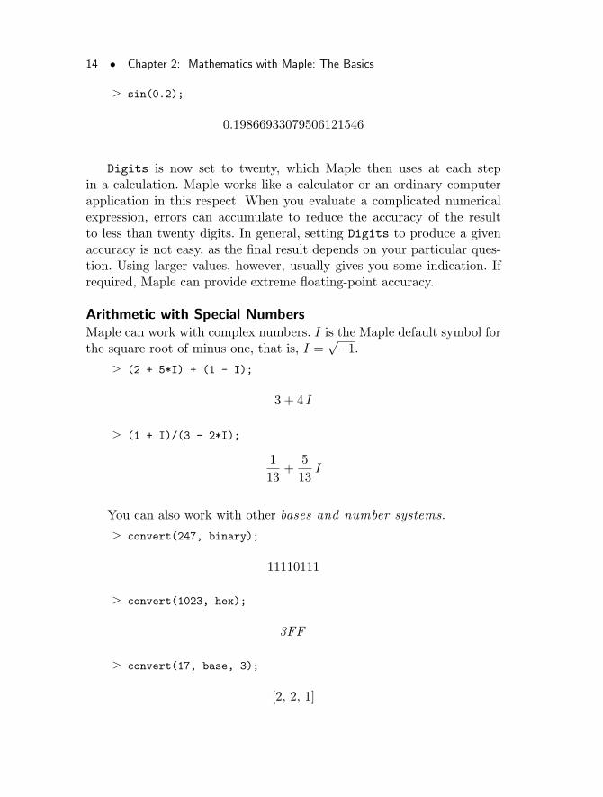
Digits is now set to twenty, which Maple then uses at each stepin a calculation. Maple works like a calculator or an ordinary computerapplication in this respect. When you evaluate a complicated numericalexpression, errors can accumulate to reduce the accuracy of the resultto less than twenty digits. In general, setting Digits to produce a givenaccuracy is not easy, as the final result depends on your particular ques-tion. Using larger values, however, usually gives you some indication. Ifrequired, Maple can provide extreme floating-point accuracy.
Arithmetic with Special NumbersMaple can work with complex numbers. I is the Maple default symbol forthe square root of minus one, that is, I =
√−1.
> (2 + 5*I) + (1 - I);
3 + 4 I
> (1 + I)/(3 - 2*I);
1
13+
5
13I
You can also work with other bases and number systems.
> convert(247, binary);
11110111
> convert(1023, hex);
3FF
> convert(17, base, 3);
[2, 2, 1]
2.2 Numerical Computations • 15
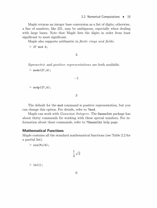
Maple returns an integer base conversion as a list of digits; otherwise,a line of numbers, like 221, may be ambiguous, especially when dealingwith large bases. Note that Maple lists the digits in order from leastsignificant to most significant.
Maple also supports arithmetic in finite rings and fields.
> 27 mod 4;
3
Symmetric and positive representations are both available.
> mods(27,4);
−1
> modp(27,4);
3
The default for the mod command is positive representation, but youcan change this option. For details, refer to ?mod.
Maple can work with Gaussian Integers . The GaussInt package hasabout thirty commands for working with these special numbers. For in-formation about these commands, refer to ?GaussInt help page.
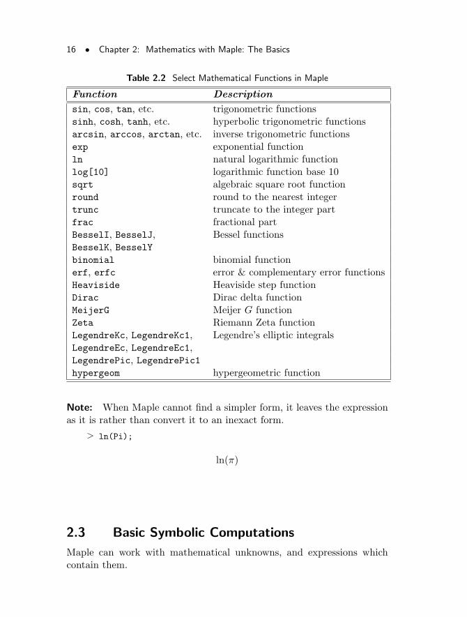
Mathematical FunctionsMaple contains all the standard mathematical functions (see Table 2.2 fora partial list).
> sin(Pi/4);
1
2
√2
> ln(1);
0
16 • Chapter 2: Mathematics with Maple: The Basics
Table 2.2 Select Mathematical Functions in Maple
Function Description
sin, cos, tan, etc. trigonometric functionssinh, cosh, tanh, etc. hyperbolic trigonometric functionsarcsin, arccos, arctan, etc. inverse trigonometric functionsexp exponential functionln natural logarithmic functionlog[10] logarithmic function base 10sqrt algebraic square root functionround round to the nearest integertrunc truncate to the integer partfrac fractional partBesselI, BesselJ, Bessel functionsBesselK, BesselYbinomial binomial functionerf, erfc error & complementary error functionsHeaviside Heaviside step functionDirac Dirac delta functionMeijerG Meijer G functionZeta Riemann Zeta functionLegendreKc, LegendreKc1, Legendre’s elliptic integralsLegendreEc, LegendreEc1,LegendrePic, LegendrePic1hypergeom hypergeometric function
Note: When Maple cannot find a simpler form, it leaves the expressionas it is rather than convert it to an inexact form.
> ln(Pi);
ln(π)
2.3 Basic Symbolic Computations
Maple can work with mathematical unknowns, and expressions whichcontain them.
2.3 Basic Symbolic Computations • 17
> (1 + x)^2;
(1 + x)2
> (1 + x) + (3 - 2*x);
4− x
Note that Maple automatically simplifies the second expression.Maple has hundreds of commands for working with symbolic expres-
sions. For a partial list, see Table 2.2.
> expand((1 + x)^2);
1 + 2x+ x2
> factor(%);
(1 + x)2
As mentioned in 2.2 Numerical Computations, the ditto operator,%, is a shorthand notation for the previous result.
> Diff(sin(x), x);
d
dxsin(x)
> value(%);
cos(x)
> Sum(n^2, n);
∑
n
n2
> value(%);
1
3n3 − 1
2n2 +
1
6n
18 • Chapter 2: Mathematics with Maple: The Basics
Divide one polynomial in x by another.
> rem(x^3+x+1, x^2+x+1, x);
2 + x
Create a series.
> series(sin(x), x=0, 10);
x− 1
6x3 +
1
120x5 − 1
5040x7 +
1
362880x9 +O(x10)
All the mathematical functions mentioned in the previous section alsoaccept unknowns as arguments.
2.4 Assigning Expressions to Names
This section introduces the following concepts in Maple.
• Naming an object
• Guidelines for Maple names
• Maple arrow notation (->)
• Assignment operator (:=)
• Predefined and reserved names
Syntax for Naming an ObjectUsing the ditto operator, or retyping a Maple expression every time youwant to use it, is not always convenient, so Maple enables you to namean object. Use the following syntax for naming.
name := expression;
You can assign any Maple expression to a name.
> var := x;
var := x
2.4 Assigning Expressions to Names • 19
> term := x*y;
term := x y
You can assign equations to names.
> eqn := x = y + 2;
eqn := x = y + 2
Guidelines for Maple NamesMaple names can include any alphanumeric characters and underscores,but they cannot start with a number. Do not start names with an un-derscore because Maple uses these names for internal classification.
• Examples of valid Maple names are polynomial, test_data, RoOt_lOcUs_pLoT,and value2.
• Examples of invalid Maple names are 2ndphase (because it beginswith a number) and x&y (because & is not an alphanumeric character).
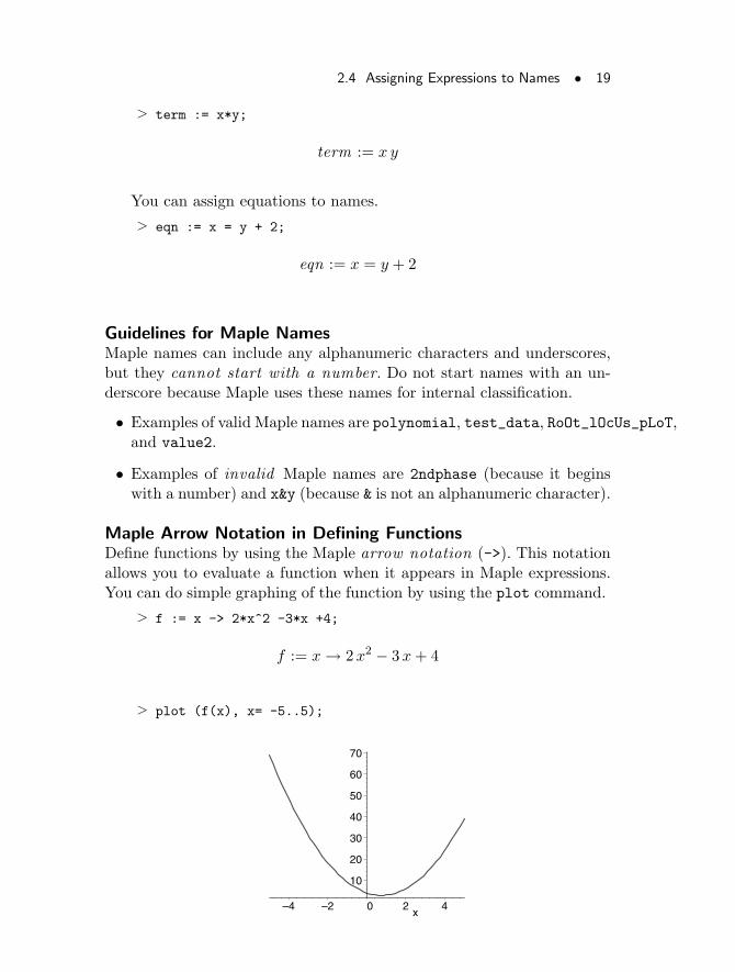
Maple Arrow Notation in Defining FunctionsDefine functions by using the Maple arrow notation (->). This notationallows you to evaluate a function when it appears in Maple expressions.You can do simple graphing of the function by using the plot command.
> f := x -> 2*x^2 -3*x +4;
f := x → 2x2 − 3x+ 4
> plot (f(x), x= -5..5);
10
20
30
40
50
60
70
–4 –2 0 2 4x
20 • Chapter 2: Mathematics with Maple: The Basics
For more information on the plot command, see chapter 5 or enter?plot at the Maple prompt.
The Assignment OperatorThe assignment (:=) operator associates a function name with a functiondefinition. The name of the function is on the left-hand side of the :=.The function definition (using the arrow notation) is on the right-handside. The following statement defines f as the squaring function.
> f := x -> x^2;
f := x → x2
Evaluating f at an argument produces the square of the argument off.
> f(5);
25
> f(y+1);
(y + 1)2
Predefined and Reserved NamesMaple has some predefined and reserved names. If you try to assign to aname that is predefined or reserved, Maple displays a message, informingyou that the name you have chosen is protected.
> Pi := 3.14;
Error, attempting to assign to ‘Pi‘ which is protected
> set := {1, 2, 3};
Error, attempting to assign to ‘set‘ which is protected
2.5 Basic Types of Maple Objects • 21
2.5 Basic Types of Maple Objects
This section examines basic types of Maple objects, including expressionsequences, lists, sets, arrays, tables, and strings. These ideas are essen-tial to the discussion in the rest of this book. Also, the following conceptsin Maple are introduced.
• Concatenation operator
• Square bracket usage
• Curly braces usage
• Mapping
• Colon (:) for suppressing output
• Double quotation mark usage
Types Expressions belong to a class or group that share common proper-ities. The classes and groups are known as types. For a complete list oftypes in Maple, refer to the ?type help page.
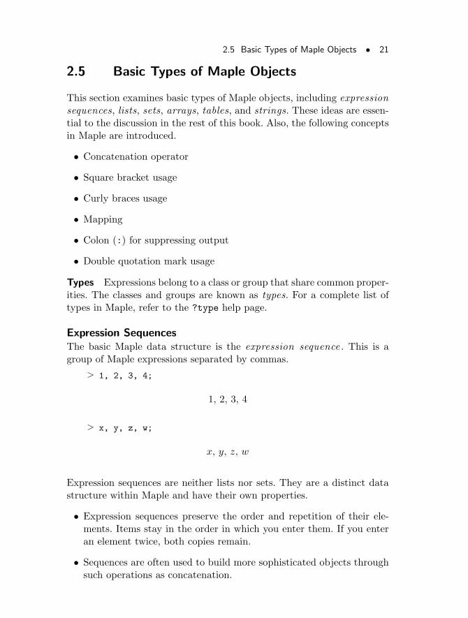
Expression SequencesThe basic Maple data structure is the expression sequence . This is agroup of Maple expressions separated by commas.
> 1, 2, 3, 4;
1, 2, 3, 4
> x, y, z, w;
x, y, z, w
Expression sequences are neither lists nor sets. They are a distinct datastructure within Maple and have their own properties.
• Expression sequences preserve the order and repetition of their ele-ments. Items stay in the order in which you enter them. If you enteran element twice, both copies remain.
• Sequences are often used to build more sophisticated objects throughsuch operations as concatenation.
22 • Chapter 2: Mathematics with Maple: The Basics
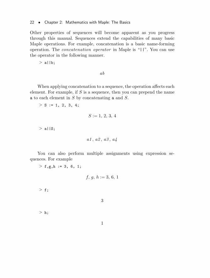
Other properties of sequences will become apparent as you progressthrough this manual. Sequences extend the capabilities of many basicMaple operations. For example, concatenation is a basic name-formingoperation. The concatenation operator in Maple is “||”. You can usethe operator in the following manner.
> a||b;
ab
When applying concatenation to a sequence, the operation affects eachelement. For example, if S is a sequence, then you can prepend the namea to each element in S by concatenating a and S.
> S := 1, 2, 3, 4;
S := 1, 2, 3, 4
> a||S;
a1 , a2 , a3 , a4
You can also perform multiple assignments using expression se-quences. For example
> f,g,h := 3, 6, 1;
f, g, h := 3, 6, 1
> f;
3
> h;
1
2.5 Basic Types of Maple Objects • 23
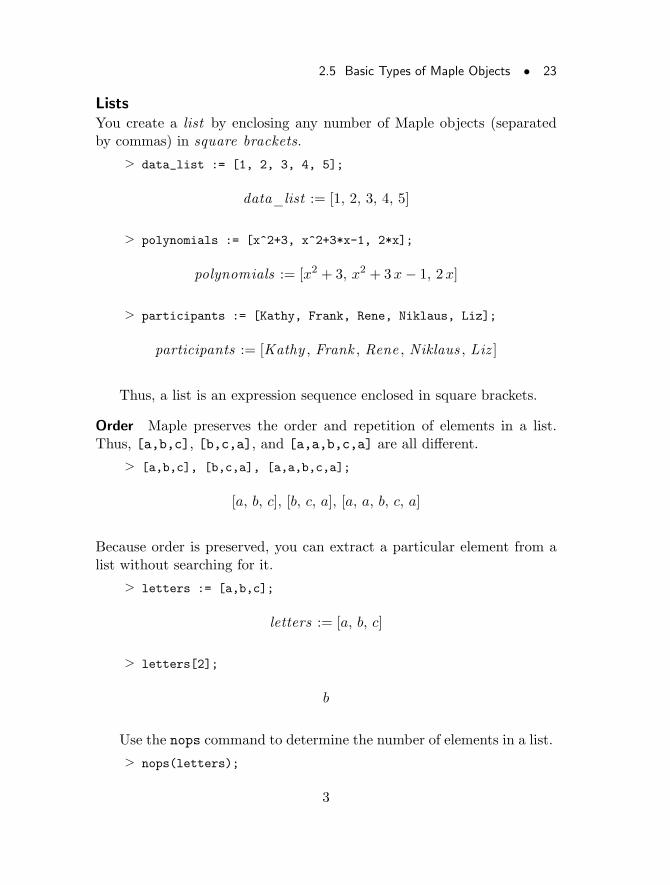
ListsYou create a list by enclosing any number of Maple objects (separatedby commas) in square brackets.
> data_list := [1, 2, 3, 4, 5];
data_list := [1, 2, 3, 4, 5]
> polynomials := [x^2+3, x^2+3*x-1, 2*x];
polynomials := [x2 + 3, x2 + 3x− 1, 2x]
> participants := [Kathy, Frank, Rene, Niklaus, Liz];
participants := [Kathy , Frank , Rene , Niklaus , Liz ]
Thus, a list is an expression sequence enclosed in square brackets.
Order Maple preserves the order and repetition of elements in a list.Thus, [a,b,c], [b,c,a], and [a,a,b,c,a] are all different.
> [a,b,c], [b,c,a], [a,a,b,c,a];
[a, b, c], [b, c, a], [a, a, b, c, a]
Because order is preserved, you can extract a particular element from alist without searching for it.
> letters := [a,b,c];
letters := [a, b, c]
> letters[2];
b
Use the nops command to determine the number of elements in a list.
> nops(letters);
3
24 • Chapter 2: Mathematics with Maple: The Basics
Section 2.6 Expression Manipulation discusses this command, in-cluding its other uses, in more detail.
Sets
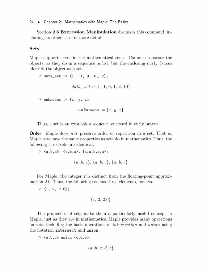
Maple supports sets in the mathematical sense. Commas separate theobjects, as they do in a sequence or list, but the enclosing curly bracesidentify the object as a set.
> data_set := {1, -1, 0, 10, 2};
data_set := {−1, 0, 1, 2, 10}
> unknowns := {x, y, z};
unknowns := {x, y, z}
Thus, a set is an expression sequence enclosed in curly braces.
Order Maple does not preserve order or repetition in a set. That is,Maple sets have the same properties as sets do in mathematics. Thus, thefollowing three sets are identical.
> {a,b,c}, {c,b,a}, {a,a,b,c,a};
{a, b, c}, {a, b, c}, {a, b, c}
For Maple, the integer 2 is distinct from the floating-point approxi-mation 2.0. Thus, the following set has three elements, not two.
> {1, 2, 2.0};
{1, 2, 2.0}
The properties of sets make them a particularly useful concept inMaple, just as they are in mathematics. Maple provides many operationson sets, including the basic operations of intersection and union usingthe notation intersect and union.
> {a,b,c} union {c,d,e};
{a, b, c, d, e}
2.5 Basic Types of Maple Objects • 25
> {1,2,3,a,b,c} intersect {0,1,y,a};
{1, a}
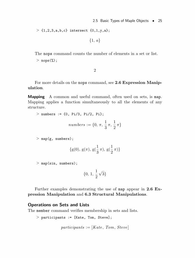
The nops command counts the number of elements in a set or list.
> nops(%);
2
For more details on the nops command, see 2.6 Expression Manip-ulation.
Mapping A common and useful command, often used on sets, is map.Mapping applies a function simultaneously to all the elements of anystructure.
> numbers := {0, Pi/3, Pi/2, Pi};
numbers := {0, π, 13π,
1
2π}
> map(g, numbers);
{g(0), g(π), g(13π), g(
1
2π)}
> map(sin, numbers);
{0, 1, 12
√3}
Further examples demonstrating the use of map appear in 2.6 Ex-pression Manipulation and 6.3 Structural Manipulations.
Operations on Sets and ListsThe member command verifies membership in sets and lists.
> participants := [Kate, Tom, Steve];
participants := [Kate , Tom, Steve ]
26 • Chapter 2: Mathematics with Maple: The Basics
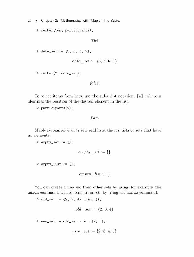
> member(Tom, participants);
true
> data_set := {5, 6, 3, 7};
data_set := {3, 5, 6, 7}
> member(2, data_set);
false
To select items from lists, use the subscript notation, [n], where nidentifies the position of the desired element in the list.
> participants[2];
Tom
Maple recognizes empty sets and lists, that is, lists or sets that haveno elements.
> empty_set := {};
empty_set := {}
> empty_list := [];
empty_list := []
You can create a new set from other sets by using, for example, theunion command. Delete items from sets by using the minus command.
> old_set := {2, 3, 4} union {};
old_set := {2, 3, 4}
> new_set := old_set union {2, 5};
new_set := {2, 3, 4, 5}
2.5 Basic Types of Maple Objects • 27
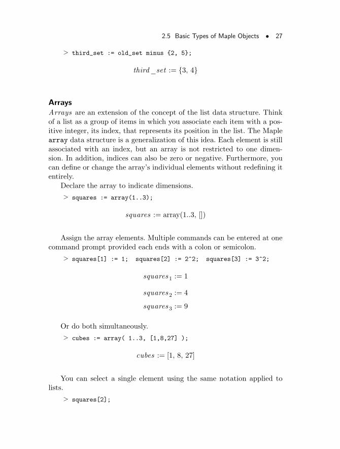
> third_set := old_set minus {2, 5};
third_set := {3, 4}
ArraysArrays are an extension of the concept of the list data structure. Thinkof a list as a group of items in which you associate each item with a pos-itive integer, its index, that represents its position in the list. The Maplearray data structure is a generalization of this idea. Each element is stillassociated with an index, but an array is not restricted to one dimen-sion. In addition, indices can also be zero or negative. Furthermore, youcan define or change the array’s individual elements without redefining itentirely.
Declare the array to indicate dimensions.
> squares := array(1..3);
squares := array(1..3, [])
Assign the array elements. Multiple commands can be entered at onecommand prompt provided each ends with a colon or semicolon.
> squares[1] := 1; squares[2] := 2^2; squares[3] := 3^2;
squares1 := 1
squares2 := 4
squares3 := 9
Or do both simultaneously.
> cubes := array( 1..3, [1,8,27] );
cubes := [1, 8, 27]
You can select a single element using the same notation applied tolists.
> squares[2];
28 • Chapter 2: Mathematics with Maple: The Basics
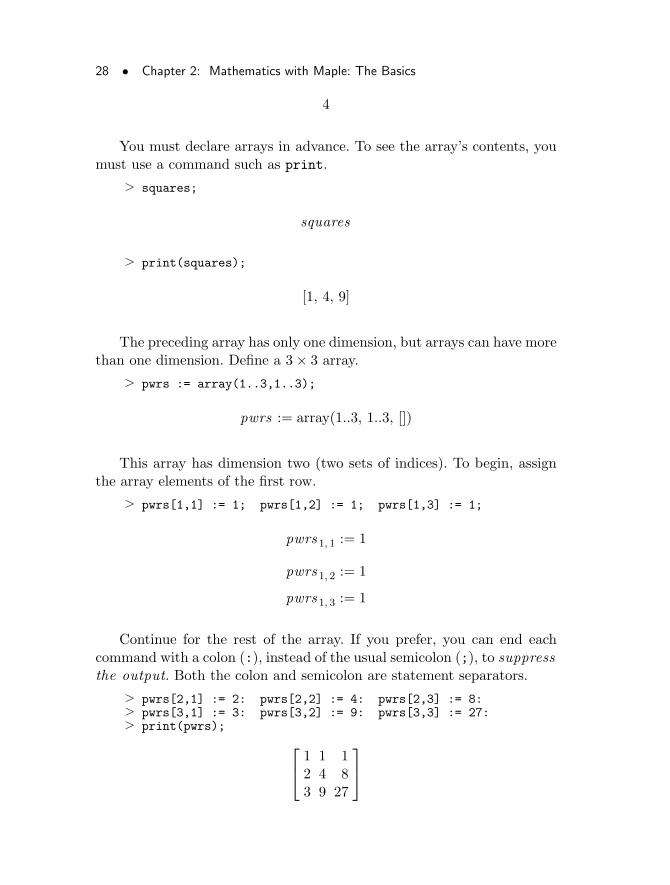
4
You must declare arrays in advance. To see the array’s contents, youmust use a command such as print.
> squares;
squares
> print(squares);
[1, 4, 9]
The preceding array has only one dimension, but arrays can have morethan one dimension. Define a 3× 3 array.
> pwrs := array(1..3,1..3);
pwrs := array(1..3, 1..3, [])
This array has dimension two (two sets of indices). To begin, assignthe array elements of the first row.
> pwrs[1,1] := 1; pwrs[1,2] := 1; pwrs[1,3] := 1;
pwrs1, 1 := 1
pwrs1, 2 := 1
pwrs1, 3 := 1
Continue for the rest of the array. If you prefer, you can end eachcommand with a colon (:), instead of the usual semicolon (;), to suppressthe output. Both the colon and semicolon are statement separators.
> pwrs[2,1] := 2: pwrs[2,2] := 4: pwrs[2,3] := 8:> pwrs[3,1] := 3: pwrs[3,2] := 9: pwrs[3,3] := 27:> print(pwrs);
1 1 12 4 83 9 27
2.5 Basic Types of Maple Objects • 29
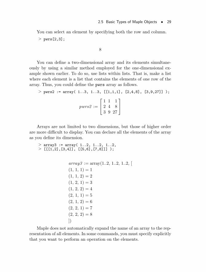
You can select an element by specifying both the row and column.
> pwrs[2,3];
8
You can define a two-dimensional array and its elements simultane-ously by using a similar method employed for the one-dimensional ex-ample shown earlier. To do so, use lists within lists. That is, make a listwhere each element is a list that contains the elements of one row of thearray. Thus, you could define the pwrs array as follows.
> pwrs2 := array( 1..3, 1..3, [[1,1,1], [2,4,8], [3,9,27]] );
pwrs2 :=
1 1 12 4 83 9 27
Arrays are not limited to two dimensions, but those of higher orderare more difficult to display. You can declare all the elements of the arrayas you define its dimension.
> array3 := array( 1..2, 1..2, 1..2,> [[[1,2],[3,4]], [[5,6],[7,8]]] );
array3 := array(1..2, 1..2, 1..2, [
(1, 1, 1) = 1
(1, 1, 2) = 2
(1, 2, 1) = 3
(1, 2, 2) = 4
(2, 1, 1) = 5
(2, 1, 2) = 6
(2, 2, 1) = 7
(2, 2, 2) = 8
])
Maple does not automatically expand the name of an array to the rep-resentation of all elements. In some commands, you must specify explicitlythat you want to perform an operation on the elements.
30 • Chapter 2: Mathematics with Maple: The Basics
Suppose that you want to define a new array identical to pwr, butwith each occurrence of the number 2 in pwrs replaced by the number 9.To perform this substitution, use the subs command. The basic syntax is
subs( x=expr1, y=expr2, ... , main_expr )
Note: The subs command does not modify the value of main_expr. Itreturns an object of the same type with the specified substitutions. Forexample, to substitute x+ y for z in an expression, do the following.
> expr := z^2 + 3;
expr := z2 + 3
> subs( {z=x+y}, expr);
(x+ y)2 + 3
Note that the following call to subs does not work.
> subs( {2=9}, pwrs );
pwrs
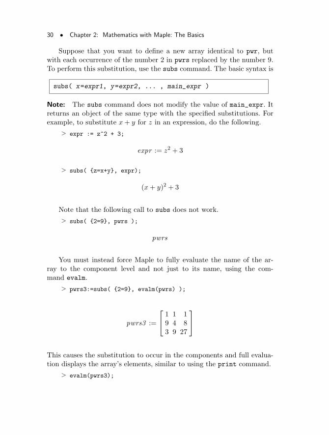
You must instead force Maple to fully evaluate the name of the ar-ray to the component level and not just to its name, using the com-mand evalm.
> pwrs3:=subs( {2=9}, evalm(pwrs) );
pwrs3 :=
1 1 19 4 83 9 27
This causes the substitution to occur in the components and full evalua-tion displays the array’s elements, similar to using the print command.
> evalm(pwrs3);
2.5 Basic Types of Maple Objects • 31
1 1 19 4 83 9 27
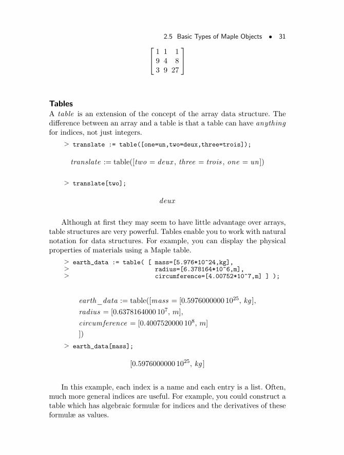
TablesA table is an extension of the concept of the array data structure. Thedifference between an array and a table is that a table can have anythingfor indices, not just integers.
> translate := table([one=un,two=deux,three=trois]);
translate := table([two = deux , three = trois , one = un])
> translate[two];
deux
Although at first they may seem to have little advantage over arrays,table structures are very powerful. Tables enable you to work with naturalnotation for data structures. For example, you can display the physicalproperties of materials using a Maple table.
> earth_data := table( [ mass=[5.976*10^24,kg],> radius=[6.378164*10^6,m],> circumference=[4.00752*10^7,m] ] );
earth_data := table([mass = [0.5976000000 1025, kg ],
radius = [0.6378164000 107, m],
circumference = [0.4007520000 108, m]
])
> earth_data[mass];
[0.5976000000 1025, kg ]
In this example, each index is a name and each entry is a list. Often,much more general indices are useful. For example, you could construct atable which has algebraic formulæ for indices and the derivatives of theseformulæ as values.
32 • Chapter 2: Mathematics with Maple: The Basics
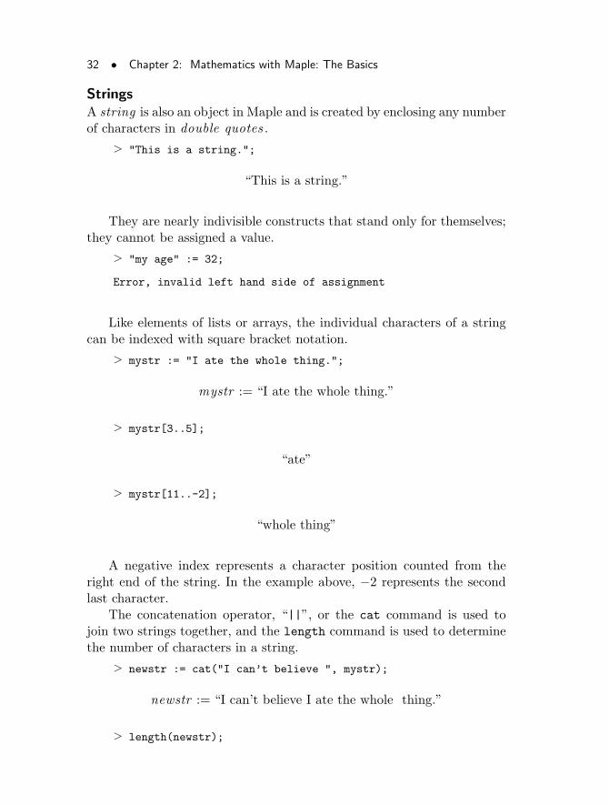
StringsA string is also an object in Maple and is created by enclosing any numberof characters in double quotes .
> "This is a string.";
“This is a string.”
They are nearly indivisible constructs that stand only for themselves;they cannot be assigned a value.
> "my age" := 32;
Error, invalid left hand side of assignment
Like elements of lists or arrays, the individual characters of a stringcan be indexed with square bracket notation.
> mystr := "I ate the whole thing.";
mystr := “I ate the whole thing.”
> mystr[3..5];
“ate”
> mystr[11..-2];
“whole thing”
A negative index represents a character position counted from theright end of the string. In the example above, −2 represents the secondlast character.
The concatenation operator, “||”, or the cat command is used tojoin two strings together, and the length command is used to determinethe number of characters in a string.
> newstr := cat("I can’t believe ", mystr);
newstr := “I can’t believe I ate the whole thing.”
> length(newstr);
2.6 Expression Manipulation • 33
38
For examples of commands that operate on strings and take stringsas input, refer to the ?StringTools help page.
2.6 Expression Manipulation
Many Maple commands concentrate on manipulating expressions. Thisincludes manipulating results of Maple commands into a familiar or usefulform. This section introduces the most commonly used commands in thisarea.
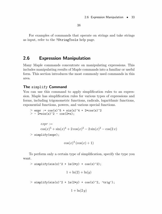
The simplify CommandYou can use this command to apply simplification rules to an expres-sion. Maple has simplification rules for various types of expressions andforms, including trigonometric functions, radicals, logarithmic functions,exponential functions, powers, and various special functions.
> expr := cos(x)^5 + sin(x)^4 + 2*cos(x)^2> - 2*sin(x)^2 - cos(2*x);
expr :=
cos(x)5 + sin(x)4 + 2 cos(x)2 − 2 sin(x)2 − cos(2x)
> simplify(expr);
cos(x)4 (cos(x) + 1)
To perform only a certain type of simplification, specify the type youwant.
> simplify(sin(x)^2 + ln(2*y) + cos(x)^2);
1 + ln(2) + ln(y)
> simplify(sin(x)^2 + ln(2*y) + cos(x)^2, ’trig’);
1 + ln(2 y)
34 • Chapter 2: Mathematics with Maple: The Basics
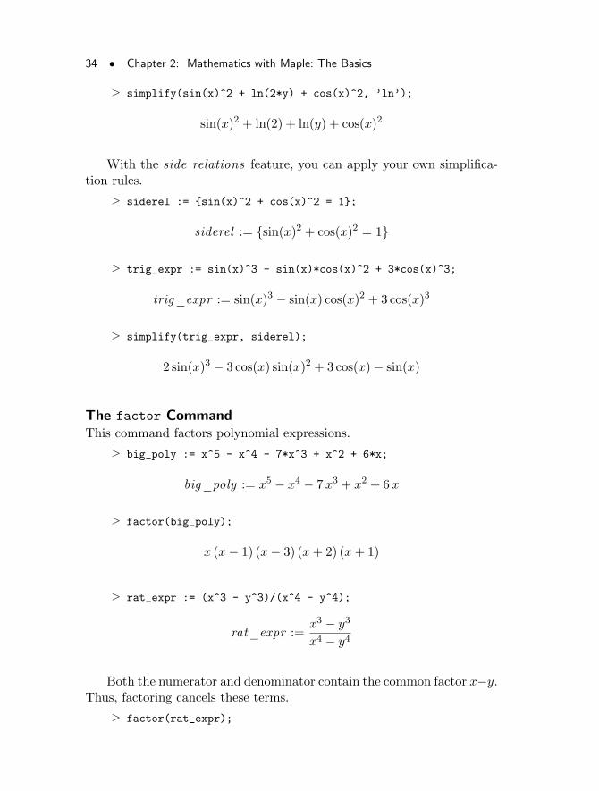
> simplify(sin(x)^2 + ln(2*y) + cos(x)^2, ’ln’);
sin(x)2 + ln(2) + ln(y) + cos(x)2
With the side relations feature, you can apply your own simplifica-tion rules.
> siderel := {sin(x)^2 + cos(x)^2 = 1};
siderel := {sin(x)2 + cos(x)2 = 1}
> trig_expr := sin(x)^3 - sin(x)*cos(x)^2 + 3*cos(x)^3;
trig_expr := sin(x)3 − sin(x) cos(x)2 + 3 cos(x)3
> simplify(trig_expr, siderel);
2 sin(x)3 − 3 cos(x) sin(x)2 + 3 cos(x)− sin(x)
The factor CommandThis command factors polynomial expressions.
> big_poly := x^5 - x^4 - 7*x^3 + x^2 + 6*x;
big_poly := x5 − x4 − 7x3 + x2 + 6x
> factor(big_poly);
x (x− 1) (x− 3) (x+ 2) (x+ 1)
> rat_expr := (x^3 - y^3)/(x^4 - y^4);
rat_expr :=x3 − y3
x4 − y4
Both the numerator and denominator contain the common factor x−y.Thus, factoring cancels these terms.
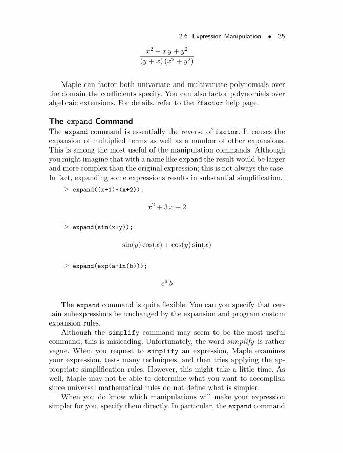
> factor(rat_expr);
2.6 Expression Manipulation • 35
x2 + x y + y2
(y + x) (x2 + y2)
Maple can factor both univariate and multivariate polynomials overthe domain the coefficients specify. You can also factor polynomials overalgebraic extensions. For details, refer to the ?factor help page.
The expand CommandThe expand command is essentially the reverse of factor. It causes theexpansion of multiplied terms as well as a number of other expansions.This is among the most useful of the manipulation commands. Althoughyou might imagine that with a name like expand the result would be largerand more complex than the original expression; this is not always the case.In fact, expanding some expressions results in substantial simplification.
> expand((x+1)*(x+2));
x2 + 3x+ 2
> expand(sin(x+y));
sin(y) cos(x) + cos(y) sin(x)
> expand(exp(a+ln(b)));
ea b
The expand command is quite flexible. You can you specify that cer-tain subexpressions be unchanged by the expansion and program customexpansion rules.
Although the simplify command may seem to be the most usefulcommand, this is misleading. Unfortunately, the word simplify is rathervague. When you request to simplify an expression, Maple examinesyour expression, tests many techniques, and then tries applying the ap-propriate simplification rules. However, this might take a little time. Aswell, Maple may not be able to determine what you want to accomplishsince universal mathematical rules do not define what is simpler.
When you do know which manipulations will make your expressionsimpler for you, specify them directly. In particular, the expand command
36 • Chapter 2: Mathematics with Maple: The Basics
is among the most useful. It frequently results in substantial simplifica-tion, and also leaves expressions in a convenient form for many othercommands.
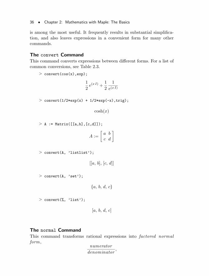
The convert CommandThis command converts expressions between different forms. For a list ofcommon conversions, see Table 2.3.
> convert(cos(x),exp);
1
2e(x I) +
1
2
1
e(x I)
> convert(1/2*exp(x) + 1/2*exp(-x),trig);
cosh(x)
> A := Matrix([[a,b],[c,d]]);
A :=
[
a bc d
]
> convert(A, ’listlist’);
[[a, b], [c, d]]
> convert(A, ’set’);
{a, b, d, c}
> convert(%, ’list’);
[a, b, d, c]
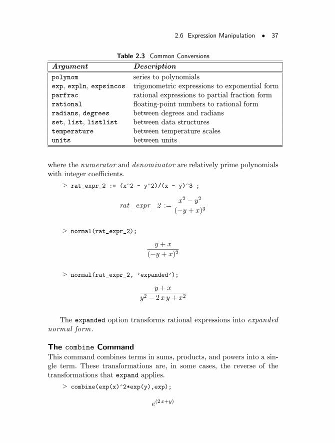
The normal CommandThis command transforms rational expressions into factored normalform,
numerator
denominator,
2.6 Expression Manipulation • 37
Table 2.3 Common Conversions
Argument Description
polynom series to polynomialsexp, expln, expsincos trigonometric expressions to exponential formparfrac rational expressions to partial fraction formrational floating-point numbers to rational formradians, degrees between degrees and radiansset, list, listlist between data structurestemperature between temperature scalesunits between units
where the numerator and denominator are relatively prime polynomialswith integer coefficients.
> rat_expr_2 := (x^2 - y^2)/(x - y)^3 ;
rat_expr_2 :=x2 − y2
(−y + x)3
> normal(rat_expr_2);
y + x
(−y + x)2
> normal(rat_expr_2, ’expanded’);
y + x
y2 − 2x y + x2
The expanded option transforms rational expressions into expandednormal form.
The combine CommandThis command combines terms in sums, products, and powers into a sin-gle term. These transformations are, in some cases, the reverse of thetransformations that expand applies.
> combine(exp(x)^2*exp(y),exp);
e(2x+y)
38 • Chapter 2: Mathematics with Maple: The Basics
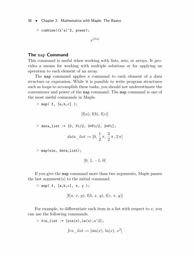
> combine((x^a)^2, power);
x(2 a)
The map CommandThis command is useful when working with lists, sets, or arrays. It pro-vides a means for working with multiple solutions or for applying anoperation to each element of an array.
The map command applies a command to each element of a datastructure or expression. While it is possible to write program structuressuch as loops to accomplish these tasks, you should not underestimate theconvenience and power of the map command. The map command is one ofthe most useful commands in Maple.
> map( f, [a,b,c] );
[f(a), f(b), f(c)]
> data_list := [0, Pi/2, 3*Pi/2, 2*Pi];
data_list := [0,1
2π,
3
2π, 2π]
> map(sin, data_list);
[0, 1, −1, 0]
If you give the map command more than two arguments, Maple passesthe last argument(s) to the initial command.
> map( f, [a,b,c], x, y );
[f(a, x, y), f(b, x, y), f(c, x, y)]
For example, to differentiate each item in a list with respect to x, youcan use the following commands.
> fcn_list := [sin(x),ln(x),x^2];
fcn_list := [sin(x), ln(x), x2]
2.6 Expression Manipulation • 39
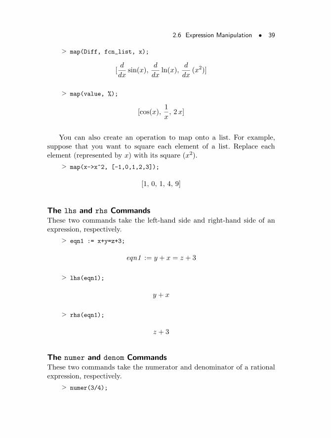
> map(Diff, fcn_list, x);
[d
dxsin(x),
d
dxln(x),
d
dx(x2)]
> map(value, %);
[cos(x),1
x, 2x]
You can also create an operation to map onto a list. For example,suppose that you want to square each element of a list. Replace eachelement (represented by x) with its square (x2).
> map(x->x^2, [-1,0,1,2,3]);
[1, 0, 1, 4, 9]
The lhs and rhs CommandsThese two commands take the left-hand side and right-hand side of anexpression, respectively.
> eqn1 := x+y=z+3;
eqn1 := y + x = z + 3
> lhs(eqn1);
y + x
> rhs(eqn1);
z + 3
The numer and denom CommandsThese two commands take the numerator and denominator of a rationalexpression, respectively.
> numer(3/4);
40 • Chapter 2: Mathematics with Maple: The Basics
3
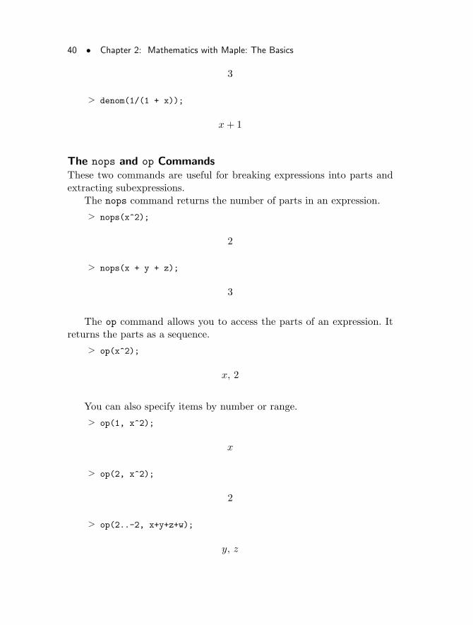
> denom(1/(1 + x));
x+ 1
The nops and op CommandsThese two commands are useful for breaking expressions into parts andextracting subexpressions.
The nops command returns the number of parts in an expression.
> nops(x^2);
2
> nops(x + y + z);
3
The op command allows you to access the parts of an expression. Itreturns the parts as a sequence.
> op(x^2);
x, 2
You can also specify items by number or range.
> op(1, x^2);
x
> op(2, x^2);
2
> op(2..-2, x+y+z+w);
y, z
2.6 Expression Manipulation • 41
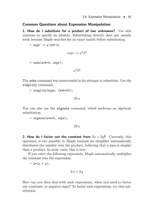
Common Questions about Expression Manipulation
1. How do I substitute for a product of two unknowns? Use siderelations to specify an identity. Substituting directly does not usuallywork because Maple searches for an exact match before substituting.
> expr := a^3*b^2;
expr := a3 b2
> subs(a*b=5, expr);
a3 b2
The subs command was unsuccessful in its attempt to substitute. Use thesimplify command.
> simplify(expr, {a*b=5});
25 a
You can also use the algsubs command, which performs an algebraicsubstitution.
> algsubs(a*b=5, expr);
25 a
2. How do I factor out the constant from 2x + 2y? Currently, thisoperation is not possible in Maple because its simplifier automaticallydistributes the number over the product, believing that a sum is simplerthan a product. In most cases, this is true.
If you enter the following expression, Maple automatically multipliesthe constant into the expression.
> 2*(x + y);
2x+ 2 y
How can you then deal with such expressions, when you need to factorout constants, or negative signs? To factor such expressions, try this sub-stitution.
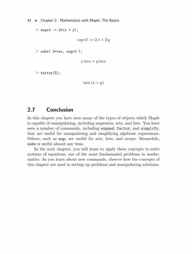
42 • Chapter 2: Mathematics with Maple: The Basics
> expr3 := 2*(x + y);
expr3 := 2x+ 2 y
> subs( 2=two, expr3 );
x two + y two
> factor(%);
two (x+ y)
2.7 Conclusion
In this chapter you have seen many of the types of objects which Mapleis capable of manipulating, including sequences, sets, and lists. You haveseen a number of commands, including expand, factor, and simplify,that are useful for manipulating and simplifying algebraic expressions.Others, such as map, are useful for sets, lists, and arrays. Meanwhile,subs is useful almost any time.
In the next chapter, you will learn to apply these concepts to solvesystems of equations, one of the most fundamental problems in mathe-matics. As you learn about new commands, observe how the concepts ofthis chapter are used in setting up problems and manipulating solutions.
3 Finding Solutions
This chapter introduces the key concepts needed for quick, concise prob-lem solving in Maple. Several commands are presented along with infor-mation on how they interoperate.
In This Chapter• Solving equations symbolically using the solve command
• Manipulations, plotting, and evaluating solutions
• Solving equations numerically using the fsolve command
• Specialized solvers in Maple
• Functions that act on polynomials
• Tools for solving problems in calculus
3.1 The Maple solve Command
The Maple solve command is a general-purpose equation solver. It takesa set of one or more equations and attempts to solve them exactly forthe specified set of unknowns. (Recall from 2.5 Basic Types of MapleObjects that you use braces to denote a set.)
Examples Using the solve CommandIn the following examples, you are solving one equation for one unknown.Each set contains only one element.
> solve({x^2=4}, {x});
43
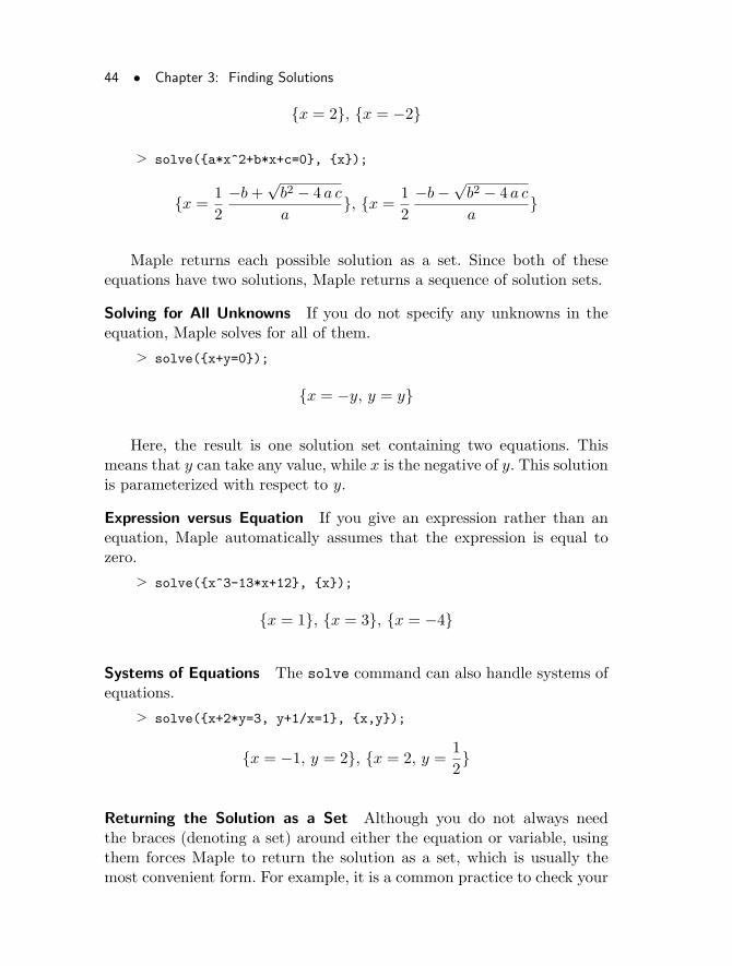
44 • Chapter 3: Finding Solutions
{x = 2}, {x = −2}
> solve({a*x^2+b*x+c=0}, {x});
{x =1
2
−b+√b2 − 4 a c
a}, {x =
1
2
−b−√b2 − 4 a c
a}
Maple returns each possible solution as a set. Since both of theseequations have two solutions, Maple returns a sequence of solution sets.
Solving for All Unknowns If you do not specify any unknowns in theequation, Maple solves for all of them.
> solve({x+y=0});
{x = −y, y = y}
Here, the result is one solution set containing two equations. Thismeans that y can take any value, while x is the negative of y. This solutionis parameterized with respect to y.
Expression versus Equation If you give an expression rather than anequation, Maple automatically assumes that the expression is equal tozero.
> solve({x^3-13*x+12}, {x});
{x = 1}, {x = 3}, {x = −4}
Systems of Equations The solve command can also handle systems ofequations.
> solve({x+2*y=3, y+1/x=1}, {x,y});
{x = −1, y = 2}, {x = 2, y =1
2}
Returning the Solution as a Set Although you do not always needthe braces (denoting a set) around either the equation or variable, usingthem forces Maple to return the solution as a set, which is usually themost convenient form. For example, it is a common practice to check your
3.1 The Maple solve Command • 45
solutions by substituting them into the original equations. The followingexample demonstrates this procedure.
As a set of equations, the solution is in an ideal form for the subs
command. You might first give the set of equations a name, like eqns, forinstance.
> eqns := {x+2*y=3, y+1/x=1};
eqns := {x+ 2 y = 3, y +1
x= 1}
Then solve.
> soln := solve( eqns, {x,y} );
soln := {x = −1, y = 2}, {x = 2, y =1
2}
This produces two solutions:
> soln[1];
{x = −1, y = 2}
and
> soln[2];
{x = 2, y =1
2}
Verifying SolutionsTo check the solutions, substitute them into the original set of equationsby using the two-parameter eval command.
> eval( eqns, soln[1] );
{1 = 1, 3 = 3}
> eval( eqns, soln[2] );
{1 = 1, 3 = 3}
46 • Chapter 3: Finding Solutions
For verifying solutions, you will find that this method is generally themost convenient.
Observe that this application of the eval command has other uses.To extract the value of x from the first solution, use the eval command.
> x1 := eval( x, soln[1] );
x1 := −1
Alternatively, you could extract the first solution for y.
> y1 := eval(y, soln[1]);
y1 := 2
Converting Solution Sets to Other Forms You can use this evaluationto convert solution sets to other forms. For example, you can constructa list from the first solution where x is the first element and y is thesecond. First construct a list with the variables in the same order asyou want the corresponding solutions.
> [x,y];
[x, y]
Evaluate this list at the first solution.
> eval([x,y], soln[1]);
[−1, 2]
The first solution is now a list.Instead, if you prefer that the solution for y comes first, evaluate [y,x]
at the solution.
> eval([y,x], soln[1]);
[2, −1]
Since Maple typically returns solutions in the form of sets (in whichthe order of objects is uncertain), remembering this method for extractingsolutions is useful.
3.1 The Maple solve Command • 47
Applying One Operation to All Solutions The map command is anotheruseful command that allows you to apply one operation to all solutions.For example, try substituting both solutions.
The map command applies the operation specified as its first argumentto its second argument.
> map(f, [a,b,c], y, z);
[f(a, y, z), f(b, y, z), f(c, y, z)]
Due to the syntactical design of map, it cannot perform multiple func-tion applications to sequences. Consider the previous solution sequence,for example,
> soln;
{x = −1, y = 2}, {x = 2, y =1
2}
Enclose soln in square brackets to convert it to a list.
> [soln];
[{x = −1, y = 2}, {x = 2, y =1
2}]
Use the following command to substitute each of the solutions simul-taneously into the original equations, eqns.
> map(subs, [soln], eqns);
[{1 = 1, 3 = 3}, {1 = 1, 3 = 3}]
This method can be valuable if your equation has many solutions,or if you are unsure of the number of solutions that a certain commandproduces.
Restricting SolutionsYou can limit solutions by specifying inequalities with the solve com-mand.
> solve({x^2=y^2},{x,y});
48 • Chapter 3: Finding Solutions
{x = −y, y = y}, {y = y, x = y}
> solve({x^2=y^2, x<>y},{x,y});
{x = −y, y = y}
Consider this system of five equations in five unknowns.
> eqn1 := x+2*y+3*z+4*t+5*u=41:> eqn2 := 5*x+5*y+4*z+3*t+2*u=20:> eqn3 := 3*y+4*z-8*t+2*u=125:> eqn4 := x+y+z+t+u=9:> eqn5 := 8*x+4*z+3*t+2*u=11:
Solve the system for all variables.
> s1 := solve({eqn1,eqn2,eqn3,eqn4,eqn5}, {x,y,z,t,u});
s1 := {x = 2, t = −11, z = −1, y = 3, u = 16}
Solving for a Subset of Unknowns You can also solve for a subset of theunknowns. Maple returns the solutions in terms of the other unknowns.
> s2 := solve({eqn1,eqn2,eqn3}, { x, y, z});
s2 := {x = −527
13− 7 t− 28
13u, z = −70
13− 7 t− 59
13u,
y =635
13+ 12 t+
70
13u}
Exploring SolutionsYou can explore the parametric solutions found at the end of the previoussection. For example, evaluate the solution at u = 1 and t = 1.
> eval( s2, {u=1,t=1} );
{x =−646
13, y =
861
13, z =
−220
13}
Suppose that you require the solutions from solve in a particularorder. Since you cannot fix the order of elements in a set, solve doesnot necessarily return your solutions in the order x, y, z. However, lists dopreserve order. Try the following.
3.1 The Maple solve Command • 49
> eval( [x,y,z], s2 );
[−527
13− 7 t− 28
13u,
635
13+ 12 t+
70
13u, −70
13− 7 t− 59
13u]
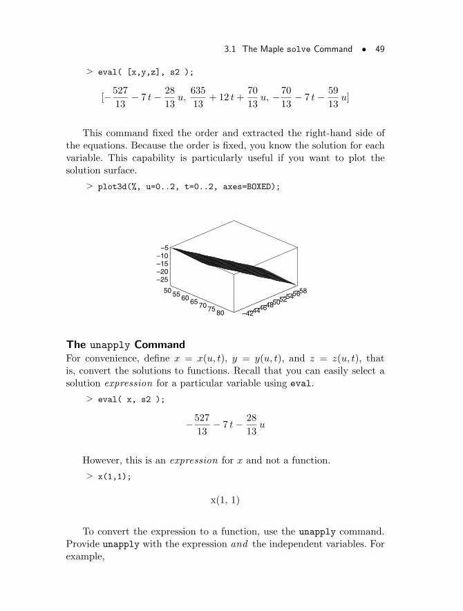
This command fixed the order and extracted the right-hand side ofthe equations. Because the order is fixed, you know the solution for eachvariable. This capability is particularly useful if you want to plot thesolution surface.
> plot3d(%, u=0..2, t=0..2, axes=BOXED);
–58–56–54–52–50–48–46–44–42
50 55 60 65 70 75 80
–25–20–15–10
–5
The unapply CommandFor convenience, define x = x(u, t), y = y(u, t), and z = z(u, t), thatis, convert the solutions to functions. Recall that you can easily select asolution expression for a particular variable using eval.
> eval( x, s2 );
−527
13− 7 t− 28
13u
However, this is an expression for x and not a function.
> x(1,1);
x(1, 1)
To convert the expression to a function, use the unapply command.Provide unapply with the expression and the independent variables. Forexample,
50 • Chapter 3: Finding Solutions
> f := unapply(x^2 + y^2 + 4, x, y);
f := (x, y) → x2 + y2 + 4
produces the function, f , of x and y that maps (x, y) to x2 + y2 + 4.This new function is easy to use.
> f(a,b);
a2 + b2 + 4
Thus, to make your solution for x a function of both u and t, obtainthe expression for x, as above.
> eval(x, s2);
−527
13− 7 t− 28
13u
Use unapply to turn it into a function of u and t.
> x := unapply(%, u, t);
x := (u, t) → −527
13− 7 t− 28
13u
> x(1,1);
−646
13
You can create the functions y and z in the same manner.
> eval(y,s2);
635
13+ 12 t+
70
13u
> y := unapply(%,u,t);
y := (u, t) → 635
13+ 12 t+
70
13u
3.1 The Maple solve Command • 51
> eval(z,s2);
−70
13− 7 t− 59
13u
> z := unapply(%, u, t);
z := (u, t) → −70
13− 7 t− 59
13u
> y(1,1), z(1,1);
861
13,−220
13
The assign CommandThe assign command allocates values to unknowns. For example, insteadof defining x, y, and z as functions, assign each to the expression on theright-hand side of the corresponding equation.
> assign( s2 );> x, y, z;
−527
13− 7 t− 28
13u,
635
13+ 12 t+
70
13u, −70
13− 7 t− 59
13u
Think of the assign command as turning the “=” signs in the solutionset into “:=” signs.
The assign command is convenient if you want to assign expressionsto names. While this command is useful for quickly assigning solu-tions, it cannot create functions.
This next example incorporates solving differential equations, whichsection 3.6 Solving Differential Equations Using the dsolve Com-mand discusses in further detail. To begin, assign the solution.
> s3 := dsolve( {diff(f(x),x)=6*x^2+1, f(0)=0}, {f(x)} );
s3 := f(x) = 2x3 + x
52 • Chapter 3: Finding Solutions
> assign( s3 );
However, you have yet to create a function.
> f(x);
2x3 + x
produces the expected answer, but despite appearances, f(x) is simplya name for the expression 2x3+x and not a function. Call the functionf using an argument other than x.
> f(1);
f(1)
The reason for this behavior is that the assign command performsthe following assignment
> f(x) := 2*x^3 + x;
f(x) := 2x3 + x
which is not the same as the assignment
> f := x -> 2*x^3 + x;
f := x → 2x3 + x
• The former defines the value of the function f for only the specialargument x.
• The latter defines the function f :x 7→ 2x3+x so that it works whetheryou say f(x), f(y), or f(1).
To define the solution f as a function of x, use unapply.
> eval(f(x),s3);
2x3 + x
> f := unapply(%, x);
3.1 The Maple solve Command • 53
f := x → 2x3 + x
> f(1);
3
The RootOf Command
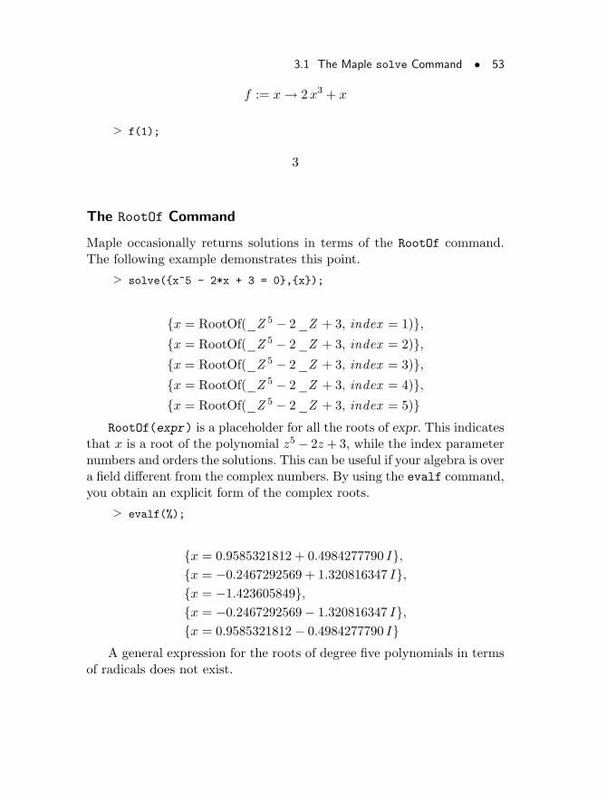
Maple occasionally returns solutions in terms of the RootOf command.The following example demonstrates this point.
> solve({x^5 - 2*x + 3 = 0},{x});
{x = RootOf(_Z 5 − 2_Z + 3, index = 1)},{x = RootOf(_Z 5 − 2_Z + 3, index = 2)},{x = RootOf(_Z 5 − 2_Z + 3, index = 3)},{x = RootOf(_Z 5 − 2_Z + 3, index = 4)},{x = RootOf(_Z 5 − 2_Z + 3, index = 5)}
RootOf(expr) is a placeholder for all the roots of expr. This indicatesthat x is a root of the polynomial z5 − 2z + 3, while the index parameternumbers and orders the solutions. This can be useful if your algebra is overa field different from the complex numbers. By using the evalf command,you obtain an explicit form of the complex roots.
> evalf(%);
{x = 0.9585321812 + 0.4984277790 I},{x = −0.2467292569 + 1.320816347 I},{x = −1.423605849},{x = −0.2467292569− 1.320816347 I},{x = 0.9585321812− 0.4984277790 I}
A general expression for the roots of degree five polynomials in termsof radicals does not exist.
54 • Chapter 3: Finding Solutions
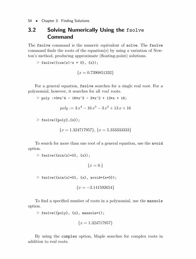
3.2 Solving Numerically Using the fsolve
Command
The fsolve command is the numeric equivalent of solve. The fsolve
command finds the roots of the equation(s) by using a variation of New-ton’s method, producing approximate (floating-point) solutions.
> fsolve({cos(x)-x = 0}, {x});
{x = 0.7390851332}
For a general equation, fsolve searches for a single real root. For apolynomial, however, it searches for all real roots.
> poly :=3*x^4 - 16*x^3 - 3*x^2 + 13*x + 16;
poly := 3x4 − 16x3 − 3x2 + 13x+ 16
> fsolve({poly},{x});
{x = 1.324717957}, {x = 5.333333333}
To search for more than one root of a general equation, use the avoidoption.
> fsolve({sin(x)=0}, {x});
{x = 0.}
> fsolve({sin(x)=0}, {x}, avoid={x=0});
{x = −3.141592654}
To find a specified number of roots in a polynomial, use the maxsols
option.
> fsolve({poly}, {x}, maxsols=1);
{x = 1.324717957}
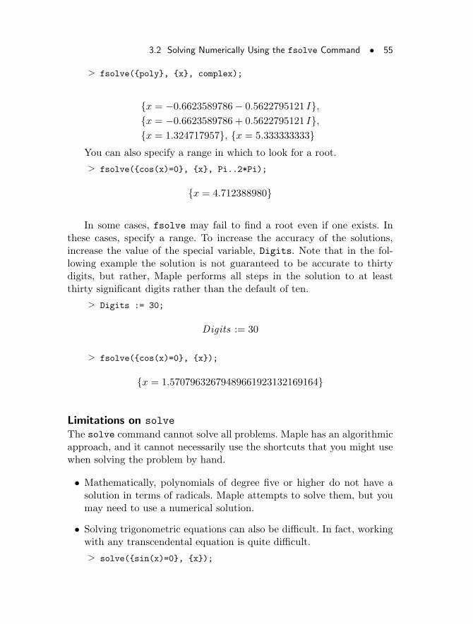
By using the complex option, Maple searches for complex roots inaddition to real roots.
3.2 Solving Numerically Using the fsolve Command • 55
> fsolve({poly}, {x}, complex);
{x = −0.6623589786− 0.5622795121 I},{x = −0.6623589786 + 0.5622795121 I},{x = 1.324717957}, {x = 5.333333333}
You can also specify a range in which to look for a root.
> fsolve({cos(x)=0}, {x}, Pi..2*Pi);
{x = 4.712388980}
In some cases, fsolve may fail to find a root even if one exists. Inthese cases, specify a range. To increase the accuracy of the solutions,increase the value of the special variable, Digits. Note that in the fol-lowing example the solution is not guaranteed to be accurate to thirtydigits, but rather, Maple performs all steps in the solution to at leastthirty significant digits rather than the default of ten.
> Digits := 30;
Digits := 30
> fsolve({cos(x)=0}, {x});
{x = 1.57079632679489661923132169164}
Limitations on solve
The solve command cannot solve all problems. Maple has an algorithmicapproach, and it cannot necessarily use the shortcuts that you might usewhen solving the problem by hand.
• Mathematically, polynomials of degree five or higher do not have asolution in terms of radicals. Maple attempts to solve them, but youmay need to use a numerical solution.
• Solving trigonometric equations can also be difficult. In fact, workingwith any transcendental equation is quite difficult.
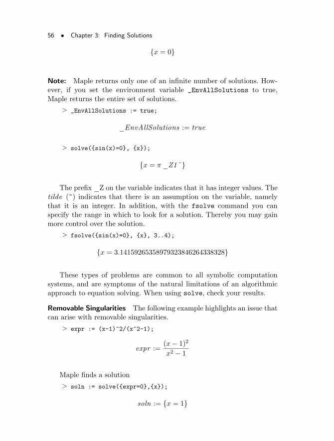
> solve({sin(x)=0}, {x});
56 • Chapter 3: Finding Solutions
{x = 0}
Note: Maple returns only one of an infinite number of solutions. How-ever, if you set the environment variable _EnvAllSolutions to true,Maple returns the entire set of solutions.
> _EnvAllSolutions := true;
_EnvAllSolutions := true
> solve({sin(x)=0}, {x});
{x = π_Z1 ~}
The prefix _Z on the variable indicates that it has integer values. Thetilde (~) indicates that there is an assumption on the variable, namelythat it is an integer. In addition, with the fsolve command you canspecify the range in which to look for a solution. Thereby you may gainmore control over the solution.
> fsolve({sin(x)=0}, {x}, 3..4);
{x = 3.14159265358979323846264338328}
These types of problems are common to all symbolic computationsystems, and are symptoms of the natural limitations of an algorithmicapproach to equation solving. When using solve, check your results.
Removable Singularities The following example highlights an issue thatcan arise with removable singularities.
> expr := (x-1)^2/(x^2-1);
expr :=(x− 1)2
x2 − 1
Maple finds a solution
> soln := solve({expr=0},{x});
soln := {x = 1}
3.2 Solving Numerically Using the fsolve Command • 57
but when you evaluate the expression at 1, you get 0/0.
> eval(expr, soln);
Error, numeric exception: division by zero
The limit shows that x = 1 is nearly a solution.
> Limit(expr, x=1);
limx→1
(x− 1)2
x2 − 1
> value (%);
0
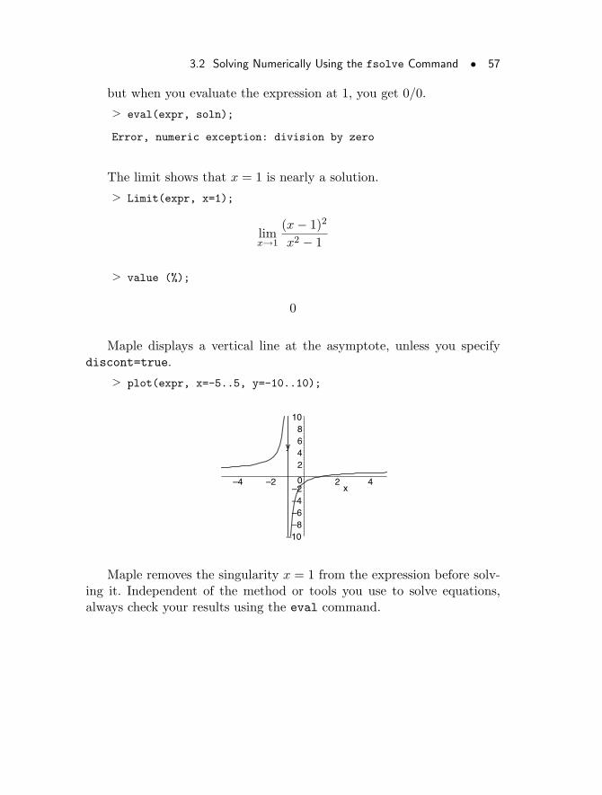
Maple displays a vertical line at the asymptote, unless you specifydiscont=true.
> plot(expr, x=-5..5, y=-10..10);
–10–8–6–4–2
0
2468
10
y
–4 –2 2 4x
Maple removes the singularity x = 1 from the expression before solv-ing it. Independent of the method or tools you use to solve equations,always check your results using the eval command.
58 • Chapter 3: Finding Solutions
3.3 Other Solvers
Maple contains many specialized solve commands. This section brieflymentions some of them. If you require more details on any of these com-mands, use the help system by entering ? and the command name at theMaple prompt.
Finding Integer SolutionsThe isolve command finds integer solutions to equations, solving for allunknowns in the expression(s).
> isolve({3*x-4*y=7});
{x = 5 + 4_Z1 , y = 2 + 3_Z1 }
Maple uses the global names _Z1, . . . , _Zn to denote the integer param-eters of the solution.
Finding Solutions Modulo mThe msolve command solves equations in the integers modulo m (thepositive representation for integers), solving for all unknowns in the ex-pression(s).
> msolve({3*x-4*y=1,7*x+y=2},17);
{y = 6, x = 14}
> msolve({2^n=3},19);
{n = 13 + 18_Z1 ~}
The tilde (~) on _Z1 indicates that msolve has placed an assumptionon _Z1, in this case that _Z1 is an integer.
> about( _Z1 );
Originally _Z1, renamed _Z1~:is assumed to be: integer
Section 6.2 Assumptions describes how you can place assumptionson unknowns.
3.4 Polynomials • 59
Solving Recurrence RelationsThe rsolve command solves recurrence equations, returning an expres-sion for the general term of the function.
> rsolve({f(n)=f(n-1)+f(n-2),f(0)=1,f(1)=1},{f(n)});
{f(n) =
(1
2+
1
10
√5) (
1
2
√5 +
1
2)n + (
1
2− 1
10
√5) (−1
2
√5 +
1
2)n}
For more information, refer to ?LREtools.
3.4 Polynomials
A polynomial in Maple is an expression containing unknowns. Each termin the polynomial contains a product of the unknowns. For example, if thepolynomial contains only one unknown, x, then the terms might containx3, x1 = x, and x0 = 1 as in the case of the polynomial x3 − 2x + 1. Ifmore than one unknown exists, then a term may also contain a productof the unknowns, as in the polynomial x3 + 3x2y + y2. Coefficients canbe integers (as in the previous examples), rational numbers, irrationalnumbers, floating-point numbers, complex numbers, or other variables.
> x^2 - 1;
x2 − 1
> x + y + z;
x+ y + z
> 1/2*x^2 - sqrt(3)*x - 1/3;
1
2x2 −
√3x− 1
3
> (1 - I)*x + 3 + 4*I;
(1− I)x+ 3 + 4 I
60 • Chapter 3: Finding Solutions
> a*x^4 + b*x^3 + c*x^2 + d*x + f;
a x4 + b x3 + c x2 + d x+ f
Maple possesses commands for many kinds of manipulations andmathematical calculations with polynomials. The following sections in-vestigate some of them.
Sorting and CollectingThe sort command arranges a polynomial into descending order of powersof the unknowns. Rather than making another copy of the polynomialwith the terms in order, sort modifies the way Maple stores the originalpolynomial in memory. In other words, if you display your polynomialafter sorting it, it retains the new order.
> sort_poly := x + x^2 - x^3 + 1 - x^4;
sort_poly := x+ x2 − x3 + 1− x4
> sort(sort_poly);
−x4 − x3 + x2 + x+ 1
> sort_poly;
−x4 − x3 + x2 + x+ 1
Maple sorts multivariate polynomials in two ways.
• The default method sorts them by total degree of the terms. Thus,x2y2 will come before both x3 and y3.
• The other option sorts by pure lexicographic order (plex), first by thepowers of the first variable in the variable list (second argument) andthen by the powers of the second variable in the variable list.
The difference between these sorts is best shown by an example.
> mul_var_poly := y^3 + x^2*y^2 + x^3;
mul_var_poly := y3 + x2 y2 + x3
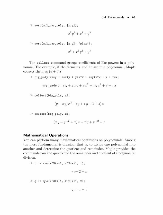
3.4 Polynomials • 61
> sort(mul_var_poly, [x,y]);
x2 y2 + x3 + y3
> sort(mul_var_poly, [x,y], ’plex’);
x3 + x2 y2 + y3
The collect command groups coefficients of like powers in a poly-nomial. For example, if the terms ax and bx are in a polynomial, Maplecollects them as (a+ b)x.
> big_poly:=x*y + z*x*y + y*x^2 - z*y*x^2 + x + z*x;
big_poly := x y + z x y + y x2 − z y x2 + x+ z x
> collect(big_poly, x);
(y − z y)x2 + (y + z y + 1 + z)x
> collect(big_poly, z);
(x y − y x2 + x) z + x y + y x2 + x
Mathematical OperationsYou can perform many mathematical operations on polynomials. Amongthe most fundamental is division, that is, to divide one polynomial intoanother and determine the quotient and remainder. Maple provides thecommands rem and quo to find the remainder and quotient of a polynomialdivision.
> r := rem(x^3+x+1, x^2+x+1, x);
r := 2 + x
> q := quo(x^3+x+1, x^2+x+1, x);
q := x− 1
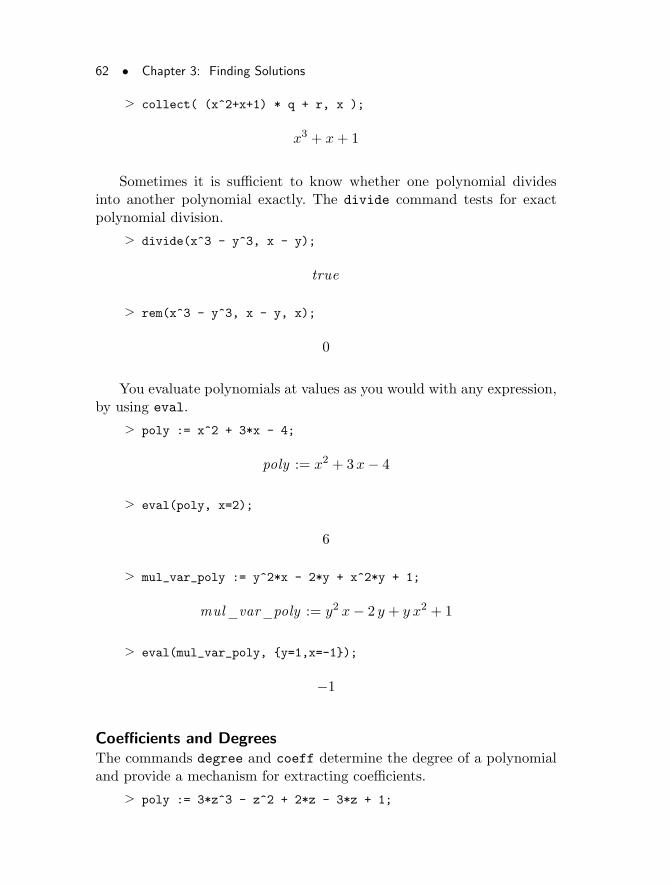
62 • Chapter 3: Finding Solutions
> collect( (x^2+x+1) * q + r, x );
x3 + x+ 1
Sometimes it is sufficient to know whether one polynomial dividesinto another polynomial exactly. The divide command tests for exactpolynomial division.
> divide(x^3 - y^3, x - y);
true
> rem(x^3 - y^3, x - y, x);
0
You evaluate polynomials at values as you would with any expression,by using eval.
> poly := x^2 + 3*x - 4;
poly := x2 + 3x− 4
> eval(poly, x=2);
6
> mul_var_poly := y^2*x - 2*y + x^2*y + 1;
mul_var_poly := y2 x− 2 y + y x2 + 1
> eval(mul_var_poly, {y=1,x=-1});
−1
Coefficients and DegreesThe commands degree and coeff determine the degree of a polynomialand provide a mechanism for extracting coefficients.
> poly := 3*z^3 - z^2 + 2*z - 3*z + 1;
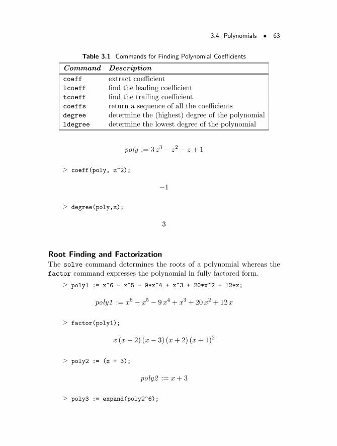
3.4 Polynomials • 63
Table 3.1 Commands for Finding Polynomial Coefficients
Command Description
coeff extract coefficientlcoeff find the leading coefficienttcoeff find the trailing coefficientcoeffs return a sequence of all the coefficientsdegree determine the (highest) degree of the polynomialldegree determine the lowest degree of the polynomial
poly := 3 z3 − z2 − z + 1
> coeff(poly, z^2);
−1
> degree(poly,z);
3
Root Finding and FactorizationThe solve command determines the roots of a polynomial whereas thefactor command expresses the polynomial in fully factored form.
> poly1 := x^6 - x^5 - 9*x^4 + x^3 + 20*x^2 + 12*x;
poly1 := x6 − x5 − 9x4 + x3 + 20x2 + 12x
> factor(poly1);
x (x− 2) (x− 3) (x+ 2) (x+ 1)2
> poly2 := (x + 3);
poly2 := x+ 3
> poly3 := expand(poly2^6);
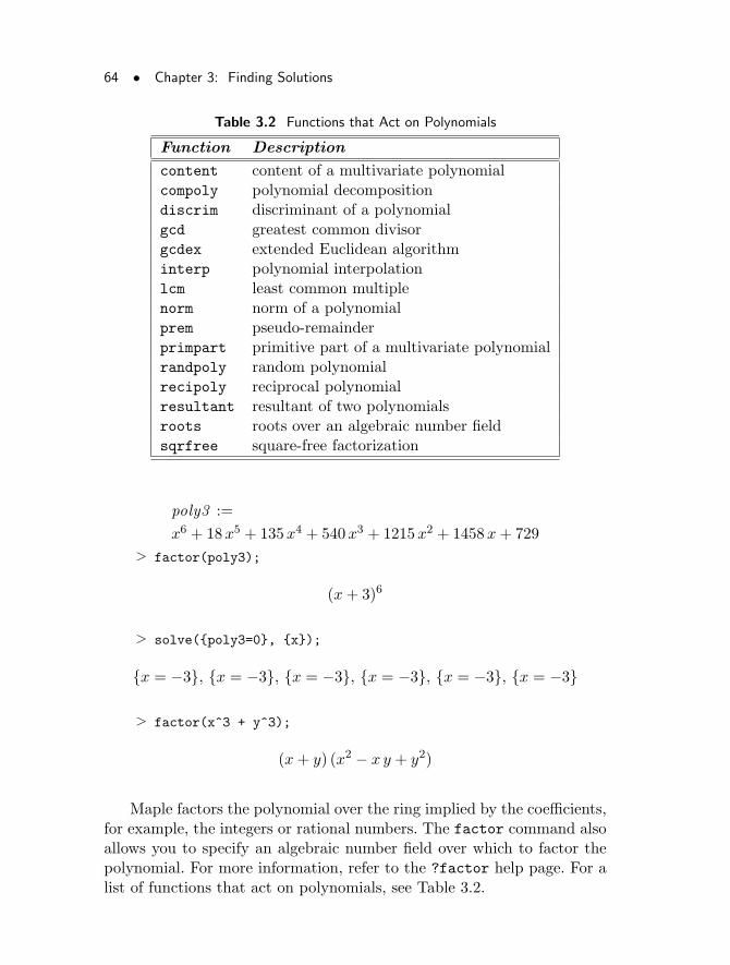
64 • Chapter 3: Finding Solutions
Table 3.2 Functions that Act on Polynomials
Function Description
content content of a multivariate polynomialcompoly polynomial decompositiondiscrim discriminant of a polynomialgcd greatest common divisorgcdex extended Euclidean algorithminterp polynomial interpolationlcm least common multiplenorm norm of a polynomialprem pseudo-remainderprimpart primitive part of a multivariate polynomialrandpoly random polynomialrecipoly reciprocal polynomialresultant resultant of two polynomialsroots roots over an algebraic number fieldsqrfree square-free factorization
poly3 :=
x6 + 18x5 + 135x4 + 540x3 + 1215x2 + 1458x+ 729
> factor(poly3);
(x+ 3)6
> solve({poly3=0}, {x});
{x = −3}, {x = −3}, {x = −3}, {x = −3}, {x = −3}, {x = −3}
> factor(x^3 + y^3);
(x+ y) (x2 − x y + y2)
Maple factors the polynomial over the ring implied by the coefficients,for example, the integers or rational numbers. The factor command alsoallows you to specify an algebraic number field over which to factor thepolynomial. For more information, refer to the ?factor help page. For alist of functions that act on polynomials, see Table 3.2.
3.5 Calculus • 65
3.5 Calculus
Maple provides many powerful tools for solving problems in calculus. Thissection presents the following concepts.
• Computing the limits of functions by using the Limit command
• Creating series approximations of a function by using the series com-mand
• Symbolically computing derivatives, indefinite integrals, and definiteintegrals
About Calculus Examples in This Manual This and the following sec-tion provide an introduction to the Maple commands for calculus prob-lems. A more extensive look at the Student[Calculus] package and thecalculus commands in the main library is provided in chapter 4 and chap-ter 7. Also, detailed information is available in the Maple help system.
Using the Limit Command Compute the limit of a rational functionas x approaches 1.
> f := x -> (x^2-2*x+1)/(x^4 + 3*x^3 - 7*x^2 + x+2);
f := x → x2 − 2x+ 1
x4 + 3x3 − 7x2 + x+ 2
> Limit(f(x), x=1);
limx→1
x2 − 2x+ 1
x4 + 3x3 − 7x2 + x+ 2
> value(%);
1
8
Taking the limit of an expression from either the positive or the neg-ative direction is also possible. For example, consider the limit of tan(x)as x approaches π/2.
Calculate the left-hand limit by using the option left.
> Limit(tan(x), x=Pi/2, left);
66 • Chapter 3: Finding Solutions
limx→(1/2π)−
tan(x)
> value(%);
∞
Calculate the right-hand limit.
> Limit(tan(x), x=Pi/2, right);
limx→(1/2π)+
tan(x)
> value(%);
−∞
Using the series Command To create a series approximation of a func-tion, note the following example.
> f := x -> sin(4*x)*cos(x);
f := x → sin(4x) cos(x)
> fs1 := series(f(x), x=0);
fs1 := 4x− 38
3x3 +
421
30x5 +O(x6)
By default, the series command generates an order 6 polynomial.By changing the value of the special variable, Order, you can increase ordecrease the order of a polynomial series.
Using convert(fs1, polynom) removes the order term from the se-ries so that Maple can plot it.
> p := convert(fs1,polynom);
p := 4x− 38
3x3 +
421
30x5
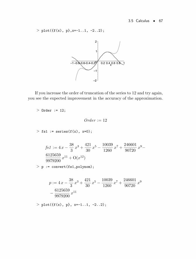
3.5 Calculus • 67
> plot({f(x), p},x=-1..1, -2..2);
–2
–1
0
1
2
–1–0.8–0.6–0.4–0.2 0.2 0.4 0.6 0.8 1x
If you increase the order of truncation of the series to 12 and try again,you see the expected improvement in the accuracy of the approximation.
> Order := 12;
Order := 12
> fs1 := series(f(x), x=0);
fs1 := 4x− 38
3x3 +
421
30x5 − 10039
1260x7 +
246601
90720x9−
6125659
9979200x11 +O(x12)
> p := convert(fs1,polynom);
p := 4x− 38
3x3 +
421
30x5 − 10039
1260x7 +
246601
90720x9
− 6125659
9979200x11
> plot({f(x), p}, x=-1..1, -2..2);
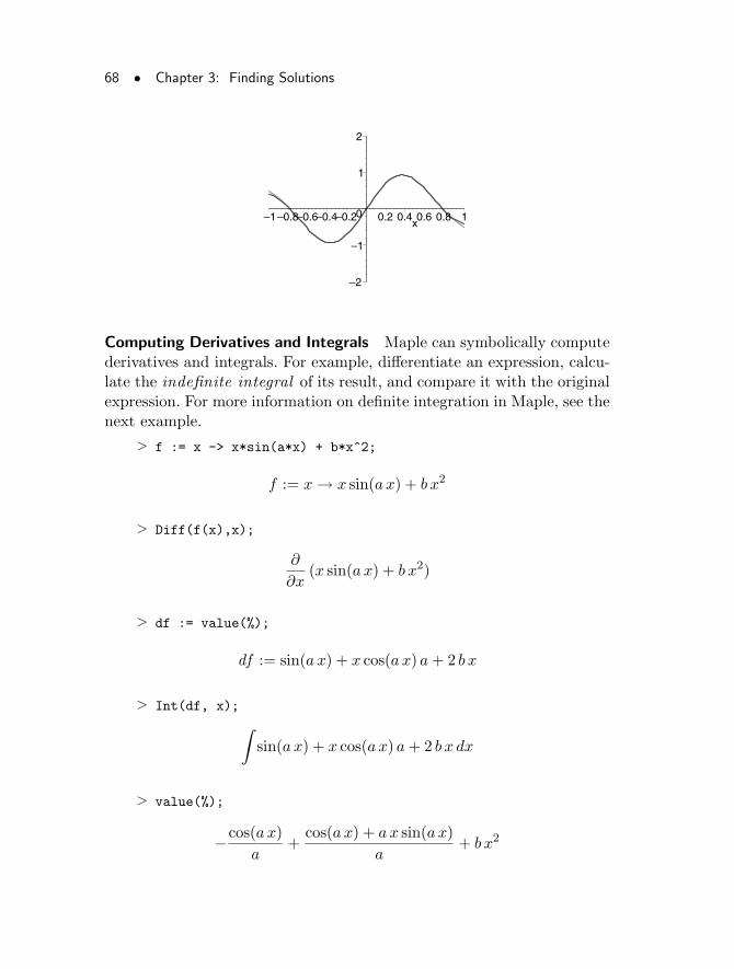
68 • Chapter 3: Finding Solutions
–2
–1
0
1
2
–1–0.8–0.6–0.4–0.2 0.2 0.4 0.6 0.8 1x
Computing Derivatives and Integrals Maple can symbolically computederivatives and integrals. For example, differentiate an expression, calcu-late the indefinite integral of its result, and compare it with the originalexpression. For more information on definite integration in Maple, see thenext example.
> f := x -> x*sin(a*x) + b*x^2;
f := x → x sin(a x) + b x2
> Diff(f(x),x);
∂
∂x(x sin(a x) + b x2)
> df := value(%);
df := sin(a x) + x cos(a x) a+ 2 b x
> Int(df, x);
∫
sin(a x) + x cos(a x) a+ 2 b x dx
> value(%);
−cos(a x)
a+
cos(a x) + a x sin(a x)
a+ b x2
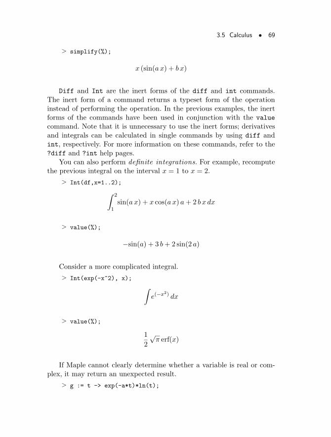
3.5 Calculus • 69
> simplify(%);
x (sin(a x) + b x)
Diff and Int are the inert forms of the diff and int commands.The inert form of a command returns a typeset form of the operationinstead of performing the operation. In the previous examples, the inertforms of the commands have been used in conjunction with the value
command. Note that it is unnecessary to use the inert forms; derivativesand integrals can be calculated in single commands by using diff andint, respectively. For more information on these commands, refer to the?diff and ?int help pages.
You can also perform definite integrations. For example, recomputethe previous integral on the interval x = 1 to x = 2.
> Int(df,x=1..2);
∫ 2
1sin(a x) + x cos(a x) a+ 2 b x dx
> value(%);
−sin(a) + 3 b+ 2 sin(2 a)
Consider a more complicated integral.
> Int(exp(-x^2), x);
∫
e(−x2) dx
> value(%);
1
2
√π erf(x)
If Maple cannot clearly determine whether a variable is real or com-plex, it may return an unexpected result.
> g := t -> exp(-a*t)*ln(t);
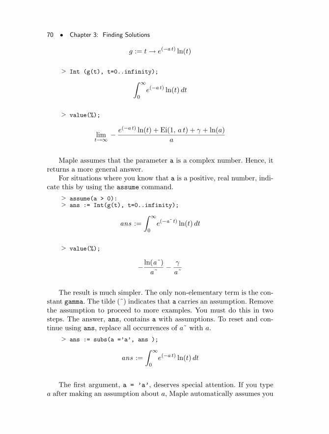
70 • Chapter 3: Finding Solutions
g := t → e(−a t) ln(t)
> Int (g(t), t=0..infinity);
∫ ∞
0e(−a t) ln(t) dt
> value(%);
limt→∞
− e(−a t) ln(t) + Ei(1, a t) + γ + ln(a)
a
Maple assumes that the parameter a is a complex number. Hence, itreturns a more general answer.
For situations where you know that a is a positive, real number, indi-cate this by using the assume command.
> assume(a > 0):> ans := Int(g(t), t=0..infinity);
ans :=
∫ ∞
0e(−a~ t) ln(t) dt
> value(%);
− ln(a~)
a~− γ
a~
The result is much simpler. The only non-elementary term is the con-stant gamma. The tilde (~) indicates that a carries an assumption. Removethe assumption to proceed to more examples. You must do this in twosteps. The answer, ans, contains a with assumptions. To reset and con-tinue using ans, replace all occurrences of a~ with a.
> ans := subs(a =’a’, ans );
ans :=
∫ ∞
0e(−a t) ln(t) dt
The first argument, a = ’a’, deserves special attention. If you typea after making an assumption about a, Maple automatically assumes you
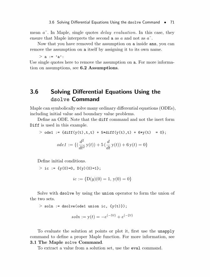
3.6 Solving Differential Equations Using the dsolve Command • 71
mean a~. In Maple, single quotes delay evaluation. In this case, theyensure that Maple interprets the second a as a and not as a~.
Now that you have removed the assumption on a inside ans, you canremove the assumption on a itself by assigning it to its own name.
> a := ’a’:
Use single quotes here to remove the assumption on a. For more informa-tion on assumptions, see 6.2 Assumptions.
3.6 Solving Differential Equations Using thedsolve Command
Maple can symbolically solve many ordinary differential equations (ODEs),including initial value and boundary value problems.
Define an ODE. Note that the diff command and not the inert formDiff is used in this example.
> ode1 := {diff(y(t),t,t) + 5*diff(y(t),t) + 6*y(t) = 0};
ode1 := {( d2
dt2y(t)) + 5 (
d
dty(t)) + 6 y(t) = 0}
Define initial conditions.
> ic := {y(0)=0, D(y)(0)=1};
ic := {D(y)(0) = 1, y(0) = 0}
Solve with dsolve by using the union operator to form the union ofthe two sets.
> soln := dsolve(ode1 union ic, {y(t)});
soln := y(t) = −e(−3 t) + e(−2 t)
To evaluate the solution at points or plot it, first use the unapply
command to define a proper Maple function. For more information, see3.1 The Maple solve Command.
To extract a value from a solution set, use the eval command.
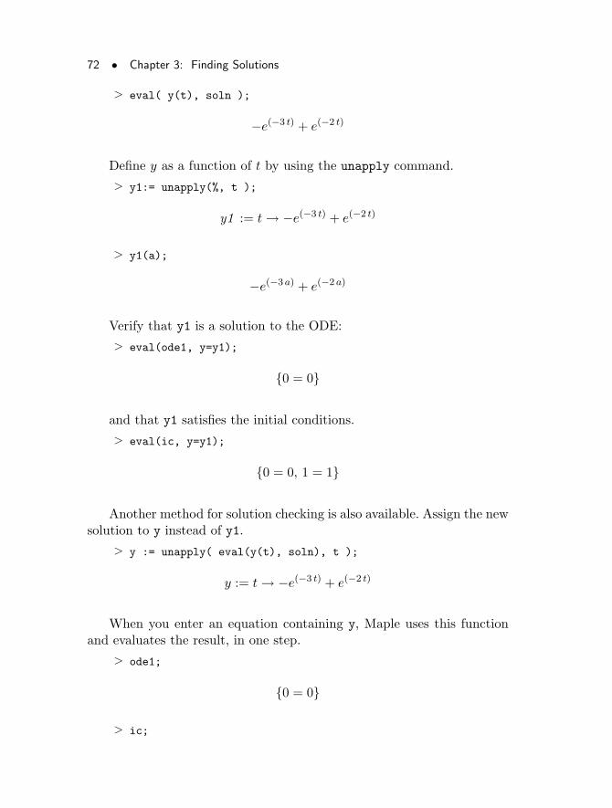
72 • Chapter 3: Finding Solutions
> eval( y(t), soln );
−e(−3 t) + e(−2 t)
Define y as a function of t by using the unapply command.
> y1:= unapply(%, t );
y1 := t → −e(−3 t) + e(−2 t)
> y1(a);
−e(−3 a) + e(−2 a)
Verify that y1 is a solution to the ODE:
> eval(ode1, y=y1);
{0 = 0}
and that y1 satisfies the initial conditions.
> eval(ic, y=y1);
{0 = 0, 1 = 1}
Another method for solution checking is also available. Assign the newsolution to y instead of y1.
> y := unapply( eval(y(t), soln), t );
y := t → −e(−3 t) + e(−2 t)
When you enter an equation containing y, Maple uses this functionand evaluates the result, in one step.
> ode1;
{0 = 0}
> ic;
3.6 Solving Differential Equations Using the dsolve Command • 73
{0 = 0, 1 = 1}
To change the differential equation, or the definition of y(t), removethe definition with the following command.
> y := ’y’;
y := y
With Maple, you can use special functions, such as the Dirac deltafunction, also called the impulse function, used in physics.
> ode2 := 10^6*diff(y(x),x,x,x,x) = Dirac(x-2) -> Dirac(x-4);
ode2 := 1000000 (d4
dx4y(x)) = Dirac(x− 2)−Dirac(x− 4)
Specify boundary conditions
> bc := {y(0)=0, D(D(y))(0)=0, y(5)=0};
bc := {y(0) = 0, y(5) = 0, (D(2))(y)(0) = 0}
and an initial value.
> iv := {D(D(y))(5)=0};
iv := {(D(2))(y)(5) = 0}
> soln := dsolve({ode2} union bc union iv, {y(x)});
74 • Chapter 3: Finding Solutions
soln := y(x) =1
6000000Heaviside(x− 2)x3
− 1
750000Heaviside(x− 2) +
1
500000Heaviside(x− 2)x
− 1
1000000Heaviside(x− 2)x2
− 1
6000000Heaviside(x− 4)x3 +
1
93750Heaviside(x− 4)
− 1
125000Heaviside(x− 4)x+
1
500000Heaviside(x− 4)x2
− 1
15000000x3 +
1
1250000x
> eval(y(x), soln);
1
6000000Heaviside(x− 2)x3 − 1
750000Heaviside(x− 2)
+1
500000Heaviside(x− 2)x
− 1
1000000Heaviside(x− 2)x2
− 1
6000000Heaviside(x− 4)x3 +
1
93750Heaviside(x− 4)
− 1
125000Heaviside(x− 4)x+
1
500000Heaviside(x− 4)x2
− 1
15000000x3 +
1
1250000x
> y := unapply(%, x);
y := x → 1
6000000Heaviside(x− 2)x3
− 1
750000Heaviside(x− 2) +
1
500000Heaviside(x− 2)x
− 1
1000000Heaviside(x− 2)x2
− 1
6000000Heaviside(x− 4)x3 +
1
93750Heaviside(x− 4)
− 1
125000Heaviside(x− 4)x+
1
500000Heaviside(x− 4)x2
− 1
15000000x3 +
1
1250000x
3.6 Solving Differential Equations Using the dsolve Command • 75
This value of y satisfies the differential equation, the boundary con-ditions, and the initial value.
> ode2;
−12Dirac(1, x− 2)− 1
6Dirac(3, x− 4)x3 + 8Dirac(2, x− 2)
+ 24Dirac(1, x− 4) + 4Dirac(x− 2)− 4Dirac(x− 4)
− 6Dirac(1, x− 4)x+ 16Dirac(2, x− 4)x
− 2Dirac(2, x− 4)x2 − 8Dirac(2, x− 2)x
+ 2Dirac(2, x− 2)x2 +1
6Dirac(3, x− 2)x3
+32
3Dirac(3, x− 4)− 4
3Dirac(3, x− 2)− 8Dirac(3, x− 4)x
+ 2Dirac(3, x− 4)x2 + 2Dirac(3, x− 2)x
−Dirac(3, x− 2)x2 + 6Dirac(1, x− 2)x
− 32Dirac(2, x− 4) = Dirac(x− 2)−Dirac(x− 4)
> simplify(%);
Dirac(x− 2)−Dirac(x− 4) = Dirac(x− 2)−Dirac(x− 4)
> bc;
{0 = 0}
> iv;
{0 = 0}
> plot(y(x), x=0..5, axes=BOXED);
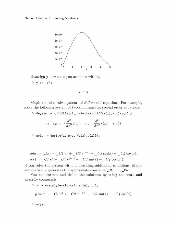
76 • Chapter 3: Finding Solutions
0
2e–07
4e–07
6e–07
8e–07
1e–06
0 1 2 3 4 5x
Unassign y now since you are done with it.
> y := ’y’;
y := y
Maple can also solve systems of differential equations. For example,solve the following system of two simultaneous, second order equations.
> de_sys := { diff(y(x),x,x)=z(x), diff(z(x),x,x)=y(x) };
de_sys := { d2
dx2z(x) = y(x),
d2
dx2y(x) = z(x)}
> soln := dsolve(de_sys, {z(x),y(x)});
soln := {z(x) = _C1 ex +_C2 e(−x) +_C3 sin(x) + _C4 cos(x),
y(x) = _C1 ex +_C2 e(−x) −_C3 sin(x)−_C4 cos(x)}If you solve the system without providing additional conditions, Mapleautomatically generates the appropriate constants _C1, . . . , _C4.
You can extract and define the solutions by using the eval andunapply commands.
> y := unapply(eval(y(x), soln), x );
y := x → _C1 ex +_C2 e(−x) −_C3 sin(x)−_C4 cos(x)
> y(1);
3.7 Conclusion • 77
_C1 e+_C2 e(−1) −_C3 sin(1)−_C4 cos(1)
You can unassign it again when you are finished.
> y := ’y’;
y := y
3.7 Conclusion
This chapter encompasses fundamental Maple features that will assistyou greatly as you learn more complicated problem-solving methods. Sec-tions 3.1 and 3.2 introduced the solve and fsolve commands, and howto evaluate and plot solutions. The final section of this chapter introducedspecialized solvers, and commands for solving calculus problems.

78 • Chapter 3: Finding Solutions
4 Maple Organization
This chapter introduces the organization of Maple, including the libraryand built-in packages of specialized commands.
In This Chapter• The Maple Library
• List of Maple Packages
• The Student Package
• The LinearAlgebra Package
• The Matlab Package
• The Statistics Package
• The simplex Linear Optimization Package
4.1 The Organization of Maple
The kernel is the base of the Maple system. It contains fundamental andprimitive commands.
• Maple language interpreter (which converts the commands you enterinto machine instructions your computer processor can understand)
• Algorithms for basic numerical calculation
• Routines to display results and perform other input and output oper-ations
79
80 • Chapter 4: Maple Organization
The kernel consists of highly optimized C code—approximately 10% ofthe system’s total size. The kernel has been kept small for speed andefficiency. The Maple kernel implements the most frequently used routinesfor integer and rational arithmetic and simple polynomial calculations.
The remaining 90% of the Maple mathematical algorithms is writtenin the Maple language and resides in the Maple library.
The Maple LibraryThe Maple library divides into two groups: the main library and thepackages. These groups of functions sit above the kernel.
The main library contains the most frequently used Maple commands(other than those in the kernel). The last commands in the library are inthe packages. Each package contains a group of commands for related cal-culations. For example, the LinearAlgebra package contains commandsfor the manipulation of Matrices.
You can use a command from a package in three ways.
1. Use the complete name of the package and the command name.
package[cmd]( ... )
If the package has a subpackage, use the complete name of the package,the complete name of the subpackage, and the command name.
package[subpackage][cmd]( ... )
2. Activate the short form of the names for all the commands in a packageby using the with command.
with(package)
If the package has a subpackage, use the following with command.
with(package[subpackage])
Then use the short name for the command.
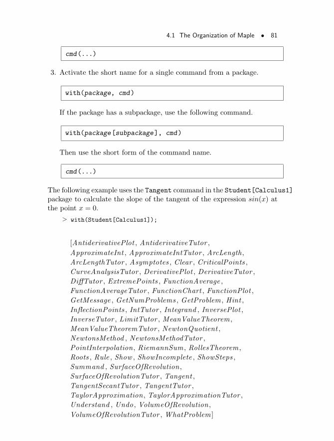
4.1 The Organization of Maple • 81
cmd(...)
3. Activate the short name for a single command from a package.
with(package, cmd)
If the package has a subpackage, use the following command.
with(package[subpackage], cmd)
Then use the short form of the command name.
cmd(...)
The following example uses the Tangent command in the Student[Calculus1]package to calculate the slope of the tangent of the expression sin(x) atthe point x = 0.
> with(Student[Calculus1]);
[AntiderivativePlot , AntiderivativeTutor ,
ApproximateInt , ApproximateIntTutor , ArcLength,
ArcLengthTutor , Asymptotes , Clear , CriticalPoints ,
CurveAnalysisTutor , DerivativePlot , DerivativeTutor ,
DiffTutor , ExtremePoints , FunctionAverage ,
FunctionAverageTutor , FunctionChart , FunctionPlot ,
GetMessage , GetNumProblems , GetProblem, Hint ,
InflectionPoints , IntTutor , Integrand , InversePlot ,
InverseTutor , LimitTutor , MeanValueTheorem,
MeanValueTheoremTutor , NewtonQuotient ,
NewtonsMethod , NewtonsMethodTutor ,
PointInterpolation, RiemannSum, RollesTheorem,
Roots , Rule , Show , ShowIncomplete , ShowSteps ,
Summand , SurfaceOfRevolution,
SurfaceOfRevolutionTutor , Tangent ,
TangentSecantTutor , TangentTutor ,
TaylorApproximation, TaylorApproximationTutor ,
Understand , Undo, VolumeOfRevolution,
VolumeOfRevolutionTutor , WhatProblem]
82 • Chapter 4: Maple Organization
> Tangent(sin(x), x = 0);
x
When you enter the with(package); command, a list of the shortforms of all command names in the package is displayed. A warning mes-sage is displayed if it has redefined any pre-existing names. To suppressthe display of the shorts forms of all command names, end the commandwith a colon, for example, with(package):.
4.2 The Maple Packages
Maple has packages of specialized commands perform tasks from an ex-tensive variety of disciplines, from Student Calculus to General RelativityTheory. The examples in this section are not intended to be comprehen-sive. They are simply examples of a few commands in selected packages,to give you a glimpse of Maple functionality.
List of PackagesMany Maple packages are listed below. For a complete list of packages, re-fer to the ?packages help page. For a full list of commands in a particularpackage, refer to the ?packagename help page.
algcurves tools for studying the one-dimensional algebraic varieties(curves) defined by multi-variate polynomials.
CodeGeneration functions that translate Maple code to other program-ming languages such as C, Fortran, JavaTM, MATLAB r©, and VisualBasic r©.
combinat combinatorial functions, including commands for calculatingpermutations and combinations of lists, and partitions of integers.(Use the combstruct package instead, where possible.)
combstruct commands for generating and counting combinatorial struc-tures, as well as determining generating function equations for suchcounting.
context tools for building and modifying context-sensitive menus in theMaple graphical user interface (for example, when right-clicking anoutput expression).
4.2 The Maple Packages • 83
CurveFitting commands that support curve-fitting.
DEtools tools for manipulating, solving, and plotting systems of differ-ential equations, phase portraits, and field plots.
diffalg commands for manipulating systems of differential polynomialequations (ODEs or PDEs).
difforms commands for handling differential forms; for problems in dif-ferential geometry.
Domains commands to create domains of computation; supports com-puting with polynomials, matrices, and series over number rings, finitefields, polynomial rings, and matrix rings.
ExternalCalling commands that link to external functions.
finance commands for financial computations.
FileTools commands for file manipulation. Contains two subpackages:Text for manipulating text files and Binary for working with files ofbinary data.
GaussInt commands for working with Gaussian Integers; that is, num-bers of the form a + bI where a and b are integers. Commands forfinding GCDs, factoring, and primality testing.
genfunc commands for manipulating rational generating functions.
geom3d commands for three-dimensional Euclidean geometry; to defineand manipulate points, lines, planes, triangles, spheres, polyhedra,etcetera, in three dimensions.
geometry commands for two-dimensional Euclidean geometry; to defineand manipulate points, lines, triangles, and circles in two dimensions.
Groebner commands for Grobner basis computations; in particular toolsfor Ore algebras and D-modules.
group commands for working with permutation groups and finitely-presented groups.
inttrans commands for working with integral transforms and their in-verses.
LibraryTools commands for library manipulation and processing.
84 • Chapter 4: Maple Organization
liesymm commands for characterizing the contact symmetries of systemsof partial differential equations.
LinearAlgebra enhanced linear algebra commands for creating specialtypes of Matrices, calculating with large numeric Matrices, and per-forming Matrix algebra.
LinearFunctionalSystems commands that solve linear functional sys-tems with polynomial coefficients, find the universal denominator ofa rational solution, and transform a matrix recurrence system into anequivalent system with a nonsingular leading or trailing matrix.
ListTools commands that manipulate lists.
LREtools commands for manipulating, plotting, and solving linear recur-rence equations.
Maplets package commands for creating windows, dialogs, and other vi-sual interfaces that interact with a user to provide the power of Maple.
MathML commands that import and export Maple expressions to and fromMathML text.
Matlab commands to use several MATLAB numerical matrix func-tions, including eigenvalues and eigenvectors, determinants, and LU-decomposition. (Only accessible if MATLAB is installed on your sys-tem.)
MatrixPolynomialAlgebra set of tools for the algebraic manipulation ofmatrix polynomials.
networks tools for constructing, drawing, and analyzing combinatorialnetworks. Facilities for handling directed graphs, and arbitrary ex-pressions for edge and vertex weights.
numapprox commands for calculating polynomial approximations to func-tions on a given interval.
numtheory commands for classic number theory, primality testing, find-ing the nth prime, factoring integers, generating cyclotomic polyno-mials. This package also contains commands for handling convergents.
Ore_algebra routines for basic computations in algebras of linear oper-ators.
4.2 The Maple Packages • 85
OrthogonalSeries commands for manipulating series of classical orthog-onal polynomials or, more generally, hypergeometric polynomials.
orthopoly commands for generating various types of orthogonal polyno-mials; useful in differential equation solving.
padic commands for computing p-adic approximations to real numbers.
PDEtools tools for manipulating, solving and plotting partial differentialequations.
plots commands for different types of specialized plots, including contourplots, two- and three-dimensional implicit plotting, plotting text, andplots in different coordinate systems.
plottools commands for generating and manipulating graphical objects.
PolynomialTools commands for manipulating polynomial objects.
powseries commands to create and manipulate formal power series rep-resented in general form.
process the commands in this package allow you to write multi-processMaple programs under UNIX r©.
RandomTools commands for working with random objects.
RationalNormalForms commands that construct the polynomial normalform or rational canonical forms of a rational function, or minimalrepresentation of a hypergeometric term.
RealDomain provides an environment in which the assumed underlyingnumber system is the real number system not the complex numbersystem.
ScientificConstants commands that provide access to the values ofvarious constant physical quantities that occur in fields such as chem-istry and physics.
ScientificErrorAnalysis commands that provide representation andconstruction of numerical quantitites that have a central value andassociated uncertainty or error. This allows users to determine theuncertainty in, for example, the product of quantities-with-error.
simplex commands for linear optimization using the simplex algorithm.
86 • Chapter 4: Maple Organization
Slode commands for finding formal power series solutions of linear ODEs.
Sockets commands for network communication in Maple. The routinesin this package enable you to connect to processes on remote hostson a network (such as an Intranet or the Internet) and exchange datawith these processes.
SolveTools commands that solve systems of algebraic equations. Thispackage gives expert users access to the routines used by the solve
command for greater control over the solution process.
Spread tools for working with spreadsheets in Maple.
stats simple statistical manipulation of data; includes averaging, stan-dard deviation, correlation coefficients, variance, and regression anal-ysis.
StringTools optimized commands for string manipulation.
Student contains subpackages that are course specific. In general, thesubpackages contain computation, interactive, and visualization com-ponents. The following is a description of three subpackages.
Precalculus interactive tutors, which help with some of the fun-damental concepts that lead to calculus.
Calculus1 commands for stepping through differentiation, integra-tion, and limit problems, visualization of Newton’s method, Rie-mann sums, arc length, volume of rotation and others, as well asroutines for finding points of interest of an expression.
LinearAlgebra commands to help instructors present and studentslearn the basic material of a standard first course in linear algebra.Visualization routines use Maple plotting facilities to represent var-ious concepts and computations, for example, displaying two 3-DVectors and their cross products. Interactive routines allow studentsto work interactively through a particular type of linear algebraproblem, such as finding the eigenvalues of a square matrix. Thesubpackage also includes routines for Matrix computations, such asconstructing a Matrix of Jordon blocks.
SumTools tools for finding closed forms of definite and indefinite sums.
tensor commands for calculating with tensors and their applications inGeneral Relativity Theory.
4.2 The Maple Packages • 87
TypeTools commands for extending the set of recognized types in thetype command.
Units commands for converting values between units, and environmentsfor performing calculations with units.
VariationalCalculus commands for Calculus of Variations computa-tions.
VectorCalculus procedures to perform multivariate and Vector calculusoperations on objects based on the rtable datatype.
Worksheet commands that provide an infrastructure for generating andmanipulating Maple worksheets by using the Maple language.
XMLTools commands that manipulate Maple’s internal representation ofXML documents.
Example PackagesThe following section provides examples from five Maple packages.
• Student[Calculus1]
• LinearAlgebra
• Matlab
• Statistics
• simplex Linear Optimization
The Student PackageThe Student package contains subpackages designed to assist with theteaching and learning of undergraduate mathematics. There are manyroutines for displaying functions, computations, and theorems. In general,the Student package contains computation, interactive, and visualizationcomponents. For a complete list of subpackages, refer to the ?Student helppage. The following provides examples from the Student[Calculus1]
subpackage.
The Student Calculus1 Subpackage (Single Variable) This subpack-age helps you step through differentiation, integration, and limit com-putations. The package contains visualization and interactive routines,and single-step computation. For details about the Student[Calculus1]package, refer to the ?Student[Calculus1] help page.
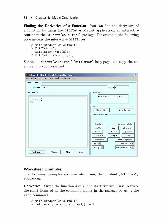
88 • Chapter 4: Maple Organization
Finding the Derivative of a Function You can find the derivative ofa function by using the DiffTutor Maplet application, an interactiveroutine in the Student[Calculus1] package. For example, the followingcode invokes the interactive DiffTutor.
> with(Student[Calculus1]);> DiffTutor();> DiffTutor(x*cos(x));> DiffTutor(x*cos(x),x);
See the ?Student[Calculus1][DiffTutor] help page and copy the ex-ample into you worksheet.
Worksheet ExamplesThe following examples are generated using the Student[Calculus1]
subpackage.
Derivative Given the function 4*x^2, find its derivative. First, activatethe short forms of all the command names in the package by using thewith command.
> with(Student[Calculus1]):> infolevel[Student[Calculus1]] := 1:
4.2 The Maple Packages • 89
To view a list of all the commands that Maple is loading, replace thecolon at the end of the command with a semicolon.
> Diff(4*x^2, x);
d
dx(4x2)
Use the constantmultiple rule.
> Rule[constantmultiple](%);
Creating problem #1
d
dx(4x2) = 4 (
d
dx(x2))
Use the power rule.
> Rule[power](%);
d
dx(4x2) = 8x
Integration Consider the following integration example. Integrate x ∗cos(x) + x from x = 0 to x = π.
> Int(x*cos(x) + x, x=0..Pi);
∫ π
0x cos(x) + x dx
Use the sum rule.
> Rule[sum](%);
Creating problem #2
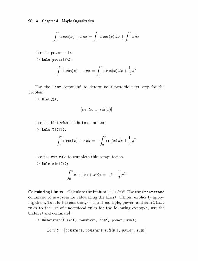
90 • Chapter 4: Maple Organization
∫ π
0x cos(x) + x dx =
∫ π
0x cos(x) dx+
∫ π
0x dx
Use the power rule.
> Rule[power](%);
∫ π
0x cos(x) + x dx =
∫ π
0x cos(x) dx+
1
2π2
Use the Hint command to determine a possible next step for theproblem.
> Hint(%);
[parts , x, sin(x)]
Use the hint with the Rule command.
> Rule[%](%%);
∫ π
0x cos(x) + x dx = −
∫ π
0sin(x) dx+
1
2π2
Use the sin rule to complete this computation.
> Rule[sin](%);
∫ π
0x cos(x) + x dx = −2 +
1
2π2
Calculating Limits Calculate the limit of (1+1/x)x. Use the Understandcommand to use rules for calculating the Limit without explicitly apply-ing them. To add the constant, constant multiple, power, and sum Limit
rules to the list of understood rules for the following example, use theUnderstand command.
> Understand(Limit, constant, ‘c*‘, power, sum);
Limit = [constant , constantmultiple , power , sum]
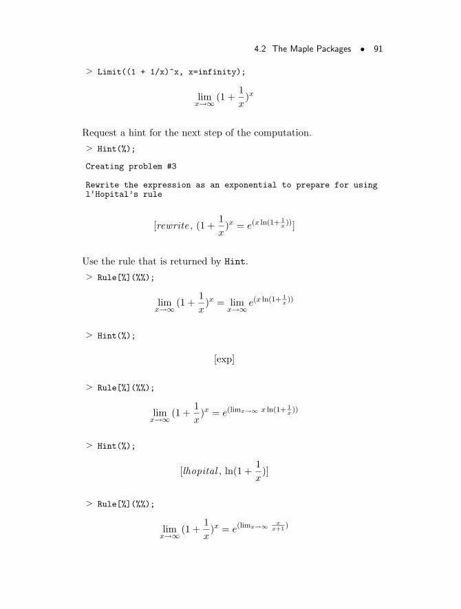
4.2 The Maple Packages • 91
> Limit((1 + 1/x)^x, x=infinity);
limx→∞
(1 +1
x)x
Request a hint for the next step of the computation.
> Hint(%);
Creating problem #3
Rewrite the expression as an exponential to prepare for usingl‘Hopital’s rule
[rewrite , (1 +1
x)x = e(x ln(1+ 1
x))]
Use the rule that is returned by Hint.
> Rule[%](%%);
limx→∞
(1 +1
x)x = lim
x→∞e(x ln(1+ 1
x))
> Hint(%);
[exp]
> Rule[%](%%);
limx→∞
(1 +1
x)x = e(limx→∞ x ln(1+ 1
x))
> Hint(%);
[lhopital , ln(1 +1
x)]
> Rule[%](%%);
limx→∞
(1 +1
x)x = e(limx→∞
xx+1 )
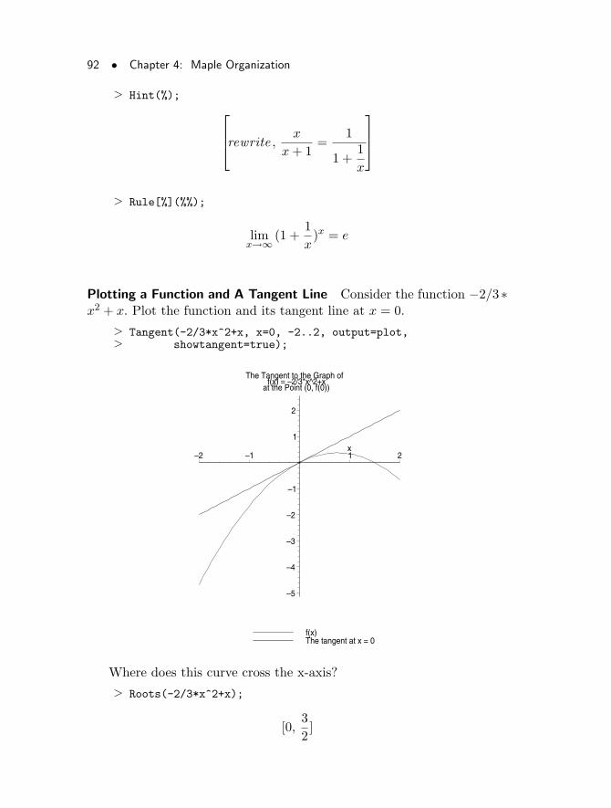
92 • Chapter 4: Maple Organization
> Hint(%);
rewrite ,x
x+ 1=
1
1 +1
x
> Rule[%](%%);
limx→∞
(1 +1
x)x = e
Plotting a Function and A Tangent Line Consider the function −2/3∗x2 + x. Plot the function and its tangent line at x = 0.
> Tangent(-2/3*x^2+x, x=0, -2..2, output=plot,> showtangent=true);
f(x)The tangent at x = 0
The Tangent to the Graph of f(x) = –2/3*x^2+x
at the Point (0, f(0))
–5
–4
–3
–2
–1
1
2
–2 –1 1 2x
Where does this curve cross the x-axis?
> Roots(-2/3*x^2+x);
[0,3
2]
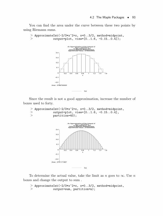
4.2 The Maple Packages • 93
You can find the area under the curve between these two points byusing Riemann sums.
> ApproximateInt(-2/3*x^2+x, x=0..3/2, method=midpoint,> output=plot, view=[0..1.6, -0.15..0.4]);
f(x)
An Approximation of the Integral off(x) = –2/3*x^2+x
on the Interval [0, 3/2]Using a Midpoint Riemann Sum
Approximate Value: .3750000000
Area: .3768750000
–0.2
–0.1
0
0.1
0.2
0.3
0.4
0.2 0.4 0.6 0.8 1 1.2 1.4 1.6x
Since the result is not a good approximation, increase the number ofboxes used to forty.
> ApproximateInt(-2/3*x^2+x, x=0..3/2, method=midpoint,> output=plot, view=[0..1.6, -0.15..0.4],> partition=40);
f(x)
An Approximation of the Integral off(x) = –2/3*x^2+x
on the Interval [0, 3/2]Using a Midpoint Riemann Sum
Approximate Value: .3750000000
Area: .3751171867
–0.2
–0.1
0
0.1
0.2
0.3
0.4
0.2 0.4 0.6 0.8 1 1.2 1.4 1.6x
To determine the actual value, take the limit as n goes to ∞. Use nboxes and change the output to sum .
> ApproximateInt(-2/3*x^2+x, x=0..3/2, method=midpoint,> output=sum, partition=n);
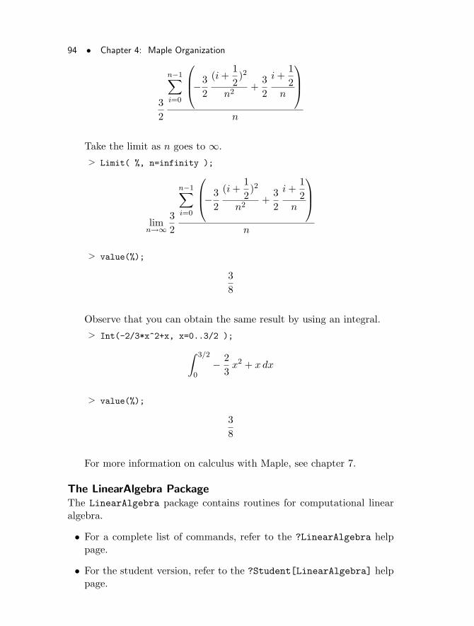
94 • Chapter 4: Maple Organization
3
2
n−1∑
i=0
−3
2
(i+1
2)2
n2+
3
2
i+1
2n
n
Take the limit as n goes to ∞.
> Limit( %, n=infinity );
limn→∞
3
2
n−1∑
i=0
−3
2
(i+1
2)2
n2+
3
2
i+1
2n
n
> value(%);
3
8
Observe that you can obtain the same result by using an integral.
> Int(-2/3*x^2+x, x=0..3/2 );
∫ 3/2
0− 2
3x2 + x dx
> value(%);
3
8
For more information on calculus with Maple, see chapter 7.
The LinearAlgebra PackageThe LinearAlgebra package contains routines for computational linearalgebra.
• For a complete list of commands, refer to the ?LinearAlgebra helppage.
• For the student version, refer to the ?Student[LinearAlgebra] helppage.
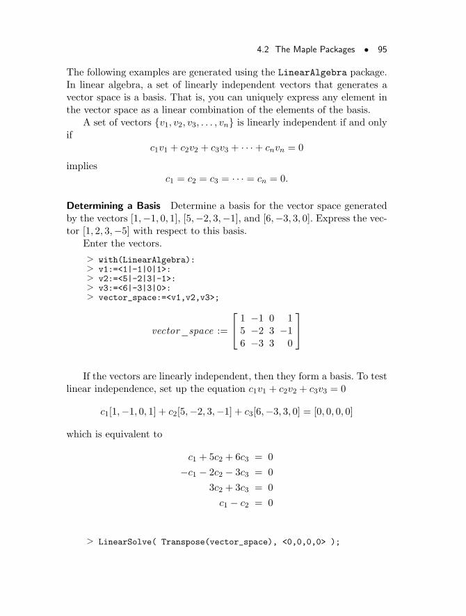
4.2 The Maple Packages • 95
The following examples are generated using the LinearAlgebra package.In linear algebra, a set of linearly independent vectors that generates avector space is a basis. That is, you can uniquely express any element inthe vector space as a linear combination of the elements of the basis.
A set of vectors {v1, v2, v3, . . . , vn} is linearly independent if and onlyif
c1v1 + c2v2 + c3v3 + · · ·+ cnvn = 0
impliesc1 = c2 = c3 = · · · = cn = 0.
Determining a Basis Determine a basis for the vector space generatedby the vectors [1,−1, 0, 1], [5,−2, 3,−1], and [6,−3, 3, 0]. Express the vec-tor [1, 2, 3,−5] with respect to this basis.
Enter the vectors.
> with(LinearAlgebra):> v1:=<1|-1|0|1>:> v2:=<5|-2|3|-1>:> v3:=<6|-3|3|0>:> vector_space:=<v1,v2,v3>;
vector_space :=
1 −1 0 15 −2 3 −16 −3 3 0
If the vectors are linearly independent, then they form a basis. To testlinear independence, set up the equation c1v1 + c2v2 + c3v3 = 0
c1[1,−1, 0, 1] + c2[5,−2, 3,−1] + c3[6,−3, 3, 0] = [0, 0, 0, 0]
which is equivalent to
c1 + 5c2 + 6c3 = 0
−c1 − 2c2 − 3c3 = 0
3c2 + 3c3 = 0
c1 − c2 = 0
> LinearSolve( Transpose(vector_space), <0,0,0,0> );
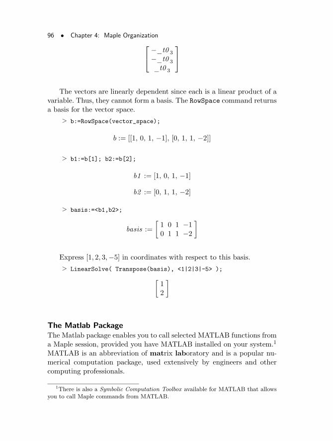
96 • Chapter 4: Maple Organization
−_t0 3
−_t0 3
_t0 3
The vectors are linearly dependent since each is a linear product of avariable. Thus, they cannot form a basis. The RowSpace command returnsa basis for the vector space.
> b:=RowSpace(vector_space);
b := [[1, 0, 1, −1], [0, 1, 1, −2]]
> b1:=b[1]; b2:=b[2];
b1 := [1, 0, 1, −1]
b2 := [0, 1, 1, −2]
> basis:=<b1,b2>;
basis :=
[
1 0 1 −10 1 1 −2
]
Express [1, 2, 3,−5] in coordinates with respect to this basis.
> LinearSolve( Transpose(basis), <1|2|3|-5> );
[
12
]
The Matlab PackageThe Matlab package enables you to call selected MATLAB functions froma Maple session, provided you have MATLAB installed on your system.1
MATLAB is an abbreviation of matrix laboratory and is a popular nu-merical computation package, used extensively by engineers and othercomputing professionals.
1There is also a Symbolic Computation Toolbox available for MATLAB that allowsyou to call Maple commands from MATLAB.
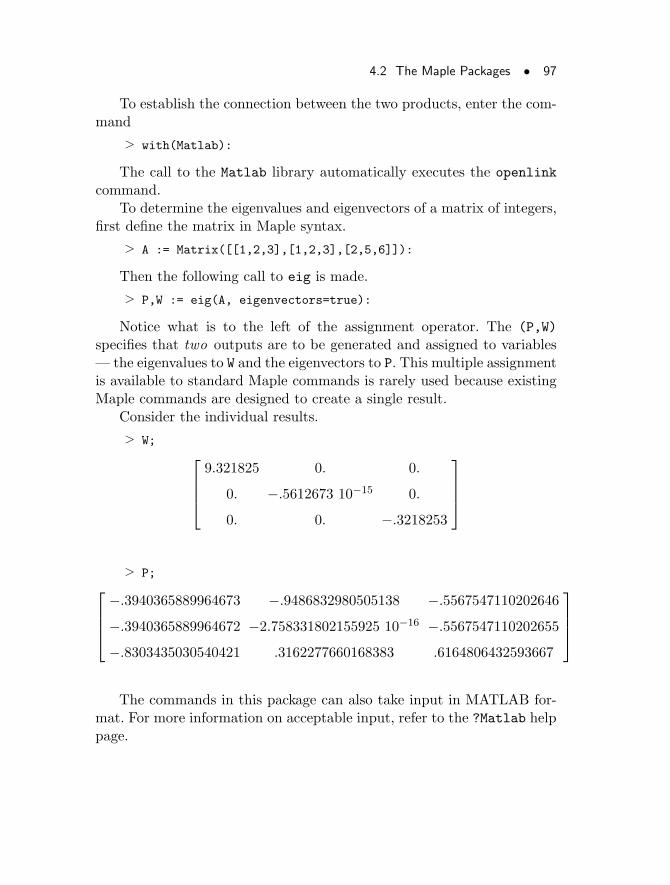
4.2 The Maple Packages • 97
To establish the connection between the two products, enter the com-mand
> with(Matlab):
The call to the Matlab library automatically executes the openlink
command.To determine the eigenvalues and eigenvectors of a matrix of integers,
first define the matrix in Maple syntax.
> A := Matrix([[1,2,3],[1,2,3],[2,5,6]]):
Then the following call to eig is made.
> P,W := eig(A, eigenvectors=true):
Notice what is to the left of the assignment operator. The (P,W)
specifies that two outputs are to be generated and assigned to variables— the eigenvalues to W and the eigenvectors to P. This multiple assignmentis available to standard Maple commands is rarely used because existingMaple commands are designed to create a single result.
Consider the individual results.
> W;
9.321825 0. 0.
0. −.5612673 10−15 0.
0. 0. −.3218253
> P;
−.3940365889964673 −.9486832980505138 −.5567547110202646
−.3940365889964672 −2.758331802155925 10−16 −.5567547110202655
−.8303435030540421 .3162277660168383 .6164806432593667
The commands in this package can also take input in MATLAB for-mat. For more information on acceptable input, refer to the ?Matlab helppage.
98 • Chapter 4: Maple Organization
The Statistics PackageThe stats package has many commands for data analysis and manipu-lation, and various types of statistical plotting. It also contains a widerange of statistical distributions.
The stats package contains subpackages. Within each subpackage,the commands are grouped by functionality.
> with(stats);
[anova, describe , fit , importdata, random, statevalf ,
statplots , transform]
The stats package works with data in statistical lists , which canbe standard Maple lists. A statistical list can also contain ranges andweighted values. The difference is best shown using an example. The namemarks is assigned a standard list,
> marks :=> [64,93,75,81,45,68,72,82,76,73];
marks := [64, 93, 75, 81, 45, 68, 72, 82, 76, 73]
as is readings
> readings := [ 0.75, 0.75, .003, 1.01, .9125,> .04, .83, 1.01, .874, .002 ];
readings := [0.75, 0.75, 0.003, 1.01, 0.9125, 0.04, 0.83,
1.01, 0.874, 0.002]
which is equivalent to the following statistical list.
> readings := [ Weight(.75, 2), .003, Weight(1.01, 2),> .9125, .04, .83, .874, .002 ];
readings := [Weight(0.75, 2), 0.003, Weight(1.01, 2),
0.9125, 0.04, 0.83, 0.874, 0.002]
The expression Weight(x,n) indicates that the value x appears ntimes in the list.
If differences less than 0.01 are so small that they are not meaningful,you can group them together, and give a range (using “..”).
4.2 The Maple Packages • 99
> readings := [ Weight(.75, 2), Weight(1.01, 2), .9125,> .04, .83, .874, Weight(0.002..0.003, 2) ];
readings := [Weight(0.75, 2), Weight(1.01, 2), 0.9125,
0.04, 0.83, 0.874, Weight(0.002..0.003, 2)]
The describe subpackage contains commands for data analysis.
> describe[mean](marks);
729
10
> describe[range](marks);
45..93
> describe[range](readings);
0.002..1.01
> describe[standarddeviation](readings);
0.4038750457
This package contains many statistical distributions. Generate somerandom data using the normal distribution, group it into ranges, and thenplot a histogram of the ranges.
> random_data:=[random[normald](50)];
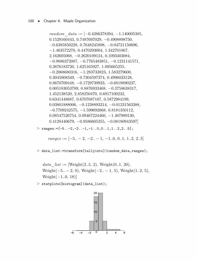
100 • Chapter 4: Maple Organization
random_data := [−0.4386378394, −1.140005385,
0.1529160443, 0.7487697029, −0.4908898750,
−0.6385850228, 0.7648245898, −0.04721150696,
−1.463572278, 0.4470293004, 1.342701867,
2.162605068, −0.2620109124, 0.1093403084,
−0.9886372087, −0.7765483851, −0.1231141571,
0.3876183720, 1.625165927, 1.095665255,
−0.2068680316, −1.283733823, 1.583279600,
0.3045008349, −0.7304597374, 0.4996033128,
0.8670709448, −0.1729739933, −0.6819890237,
0.005183053789, 0.8876933468, −0.3758638317,
1.452138520, 2.858250470, 0.6917100232,
0.6341448687, 0.6707087107, 0.5872984199,
0.03801888006, −0.1238893314, −0.01231563388,
−0.7709242575, −1.599692668, 0.8181350112,
0.08547526754, 0.09467224460, −1.407989130,
0.4128440679, −0.9586605355, −0.08180943597]
> ranges:=[-5..-2,-2..-1,-1..0,0..1,1..2,2..5];
ranges := [−5..− 2, −2..− 1, −1..0, 0..1, 1..2, 2..5]
> data_list:=transform[tallyinto](random_data,ranges);
data_list := [Weight(2..5, 2), Weight(0..1, 20),
Weight(−5..− 2, 0), Weight(−2..− 1, 5), Weight(1..2, 5),
Weight(−1..0, 18)]
> statplots[histogram](data_list);
0
5
10
15
20
–6 –4 –2 2 4 6
4.2 The Maple Packages • 101
The simplex Linear Optimization PackageThe simplex package contains commands for linear optimization, usingthe simplex algorithm. Linear optimization involves finding optimal solu-tions to equations under constraints.
An example of a classic optimization problem is the pizza deliveryproblem. You have four pizzas to deliver, to four different places, spreadthroughout the city. You want to deliver all four using as little gas aspossible. You also must get to all four locations in under twenty minutes,so that the pizzas stay hot. If you can create mathematical equationsrepresenting the routes to the four places and the distances, you can findthe optimal solution. That is, you can determine what route you shouldtake to get to all four places in as little time and using as little gas aspossible. The constraints on this particular system are that you have todeliver all four pizzas within twenty minutes of leaving the restaurant.
Here is a very small system as an example.
> with(simplex);
Warning, the name basis has been redefinedWarning, the protected names maximize and minimize havebeen redefined and unprotected
[basis , convexhull , cterm, define_zero, display , dual ,
feasible , maximize , minimize , pivot , pivoteqn, pivotvar ,
ratio, setup, standardize ]
To maximize the expression w, enter
> w := -x+y+2*z;
w := −x+ y + 2 z
subject to the constraints c1, c2, and c3.
> c1 := 3*x+4*y-3*z <= 23;
c1 := 3x+ 4 y − 3 z ≤ 23
> c2 := 5*x-4*y-3*z <= 10;
c2 := 5x− 4 y − 3 z ≤ 10
102 • Chapter 4: Maple Organization
> c3 := 7*x +4*y+11*z <= 30;
c3 := 7x+ 4 y + 11 z ≤ 30
> maximize(w, {c1,c2,c3});
In this case, no answer means that Maple cannot find a solution. You canuse the feasible command to determine if the set of constraints is valid.
> feasible({c1,c2,c3});
true
Try again and place an additional restriction on the solution.
> maximize(w, {c1,c2,c3}, NONNEGATIVE);
{z =1
2, y =
49
8, x = 0}
4.3 Conclusion
This chapter introduced the organization of Maple and the Maple library.Additionally, examples from five packages were provided. This informationserves as context for references and concepts in the following chapters.
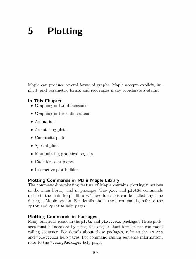
5 Plotting
Maple can produce several forms of graphs. Maple accepts explicit, im-plicit, and parametric forms, and recognizes many coordinate systems.
In This Chapter• Graphing in two dimensions
• Graphing in three dimensions
• Animation
• Annotating plots
• Composite plots
• Special plots
• Manipulating graphical objects
• Code for color plates
• Interactive plot builder
Plotting Commands in Main Maple LibraryThe command-line plotting feature of Maple contains plotting functionsin the main library and in packages. The plot and plot3d commandsreside in the main Maple library. These functions can be called any timeduring a Maple session. For details about these commands, refer to the?plot and ?plot3d help pages.
Plotting Commands in PackagesMany functions reside in the plots and plottools packages. These pack-ages must be accessed by using the long or short form in the commandcalling sequence. For details about these packages, refer to the ?plots
and ?plottools help pages. For command calling sequence information,refer to the ?UsingPackages help page.
103
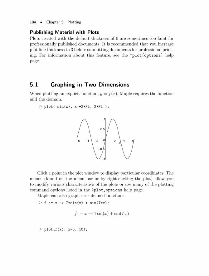
104 • Chapter 5: Plotting
Publishing Material with PlotsPlots created with the default thickness of 0 are sometimes too faint forprofessionally published documents. It is recommended that you increaseplot line thickness to 3 before submitting documents for professional print-ing. For information about this feature, see the ?plot[options] helppage.
5.1 Graphing in Two Dimensions
When plotting an explicit function, y = f(x), Maple requires the functionand the domain.
> plot( sin(x), x=-2*Pi..2*Pi );
–1
–0.5
0
0.5
1
–6 –4 –2 2 4 6x
Click a point in the plot window to display particular coordinates. Themenus (found on the menu bar or by right-clicking the plot) allow youto modify various characteristics of the plots or use many of the plottingcommand options listed in the ?plot,options help page.
Maple can also graph user-defined functions.
> f := x -> 7*sin(x) + sin(7*x);
f := x → 7 sin(x) + sin(7x)
> plot(f(x), x=0..10);
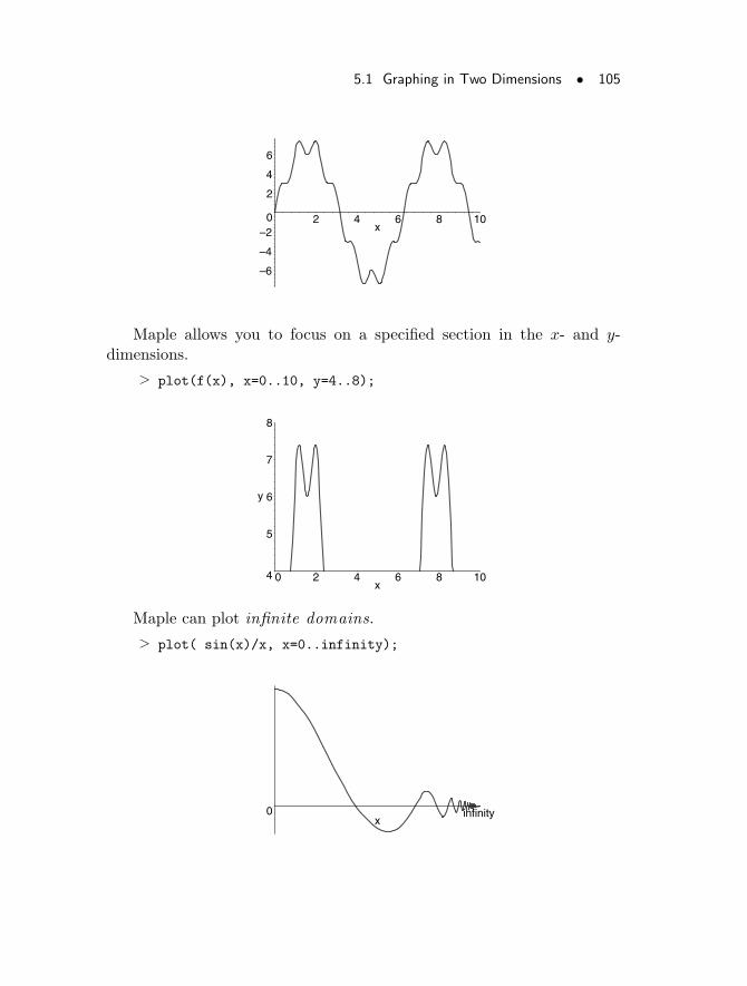
5.1 Graphing in Two Dimensions • 105
–6
–4
–20
2
4
6
2 4 6 8 10x
Maple allows you to focus on a specified section in the x- and y-dimensions.
> plot(f(x), x=0..10, y=4..8);
4
5
6
7
8
y
0 2 4 6 8 10x
Maple can plot infinite domains.
> plot( sin(x)/x, x=0..infinity);
0 infinityx
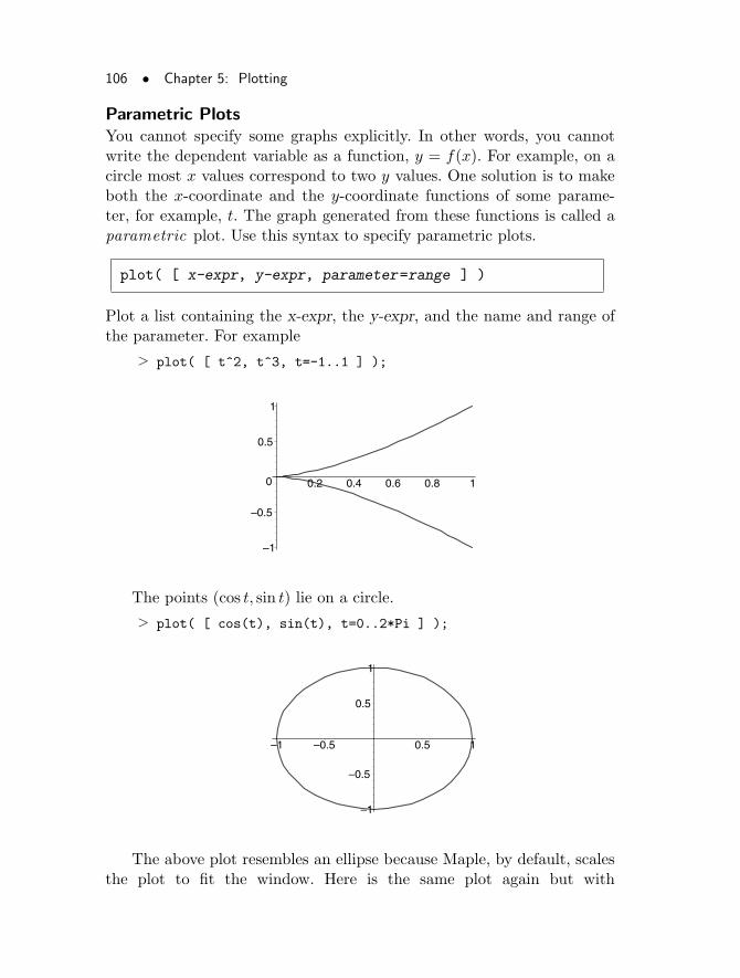
106 • Chapter 5: Plotting
Parametric PlotsYou cannot specify some graphs explicitly. In other words, you cannotwrite the dependent variable as a function, y = f(x). For example, on acircle most x values correspond to two y values. One solution is to makeboth the x-coordinate and the y-coordinate functions of some parame-ter, for example, t. The graph generated from these functions is called aparametric plot. Use this syntax to specify parametric plots.
plot( [ x-expr, y-expr, parameter=range ] )
Plot a list containing the x-expr, the y-expr, and the name and range ofthe parameter. For example
> plot( [ t^2, t^3, t=-1..1 ] );
–1
–0.5
0
0.5
1
0.2 0.4 0.6 0.8 1
The points (cos t, sin t) lie on a circle.
> plot( [ cos(t), sin(t), t=0..2*Pi ] );
–1
–0.5
0.5
1
–1 –0.5 0.5 1
The above plot resembles an ellipse because Maple, by default, scalesthe plot to fit the window. Here is the same plot again but with
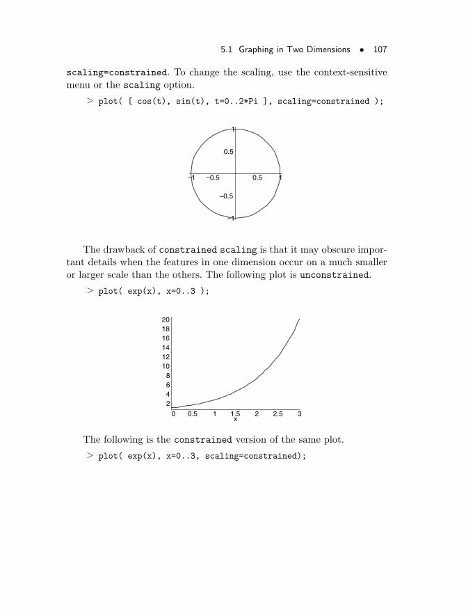
5.1 Graphing in Two Dimensions • 107
scaling=constrained. To change the scaling, use the context-sensitivemenu or the scaling option.
> plot( [ cos(t), sin(t), t=0..2*Pi ], scaling=constrained );
–1
–0.5
0.5
1
–1 –0.5 0.5 1
The drawback of constrained scaling is that it may obscure impor-tant details when the features in one dimension occur on a much smalleror larger scale than the others. The following plot is unconstrained.
> plot( exp(x), x=0..3 );
2468
101214161820
0 0.5 1 1.5 2 2.5 3x
The following is the constrained version of the same plot.
> plot( exp(x), x=0..3, scaling=constrained);
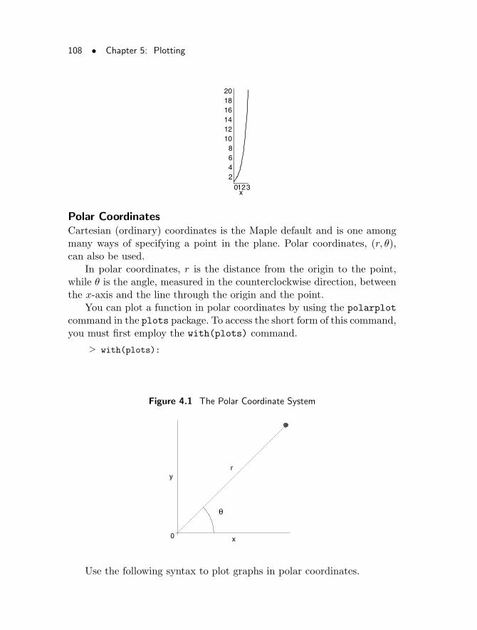
108 • Chapter 5: Plotting
2468
101214161820
0123x
Polar CoordinatesCartesian (ordinary) coordinates is the Maple default and is one amongmany ways of specifying a point in the plane. Polar coordinates, (r, θ),can also be used.
In polar coordinates, r is the distance from the origin to the point,while θ is the angle, measured in the counterclockwise direction, betweenthe x-axis and the line through the origin and the point.
You can plot a function in polar coordinates by using the polarplot
command in the plots package. To access the short form of this command,you must first employ the with(plots) command.
> with(plots):
Figure 4.1 The Polar Coordinate System
θ
r
0
y
x
Use the following syntax to plot graphs in polar coordinates.
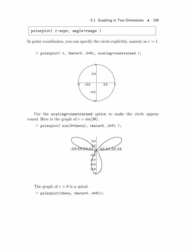
5.1 Graphing in Two Dimensions • 109
polarplot( r-expr, angle=range )
In polar coordinates, you can specify the circle explicitly, namely as r = 1.
> polarplot( 1, theta=0..2*Pi, scaling=constrained );
–1
–0.5
0.5
1
–1 –0.5 0.5 1
Use the scaling=constrained option to make the circle appearround. Here is the graph of r = sin(3θ).
> polarplot( sin(3*theta), theta=0..2*Pi );
–1
–0.8
–0.6
–0.4
–0.20
0.2
0.4
–0.8–0.6–0.4–0.2 0.2 0.4 0.6 0.8
The graph of r = θ is a spiral.
> polarplot(theta, theta=0..4*Pi);
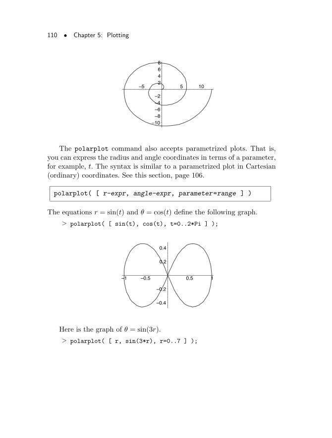
110 • Chapter 5: Plotting
–10–8–6–4–2
2468
–5 5 10
The polarplot command also accepts parametrized plots. That is,you can express the radius and angle coordinates in terms of a parameter,for example, t. The syntax is similar to a parametrized plot in Cartesian(ordinary) coordinates. See this section, page 106.
polarplot( [ r-expr, angle-expr, parameter=range ] )
The equations r = sin(t) and θ = cos(t) define the following graph.
> polarplot( [ sin(t), cos(t), t=0..2*Pi ] );
–0.4
–0.2
0.2
0.4
–1 –0.5 0.5 1
Here is the graph of θ = sin(3r).
> polarplot( [ r, sin(3*r), r=0..7 ] );
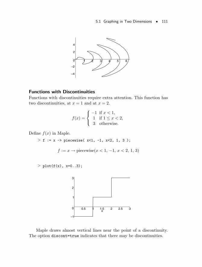
5.1 Graphing in Two Dimensions • 111
–4
–2
0
2
4
1 2 3 4 5 6
Functions with DiscontinuitiesFunctions with discontinuities require extra attention. This function hastwo discontinuities, at x = 1 and at x = 2.
f(x) =
−1 if x < 1,1 if 1 ≤ x < 2,3 otherwise.
Define f(x) in Maple.
> f := x -> piecewise( x<1, -1, x<2, 1, 3 );
f := x → piecewise(x < 1, −1, x < 2, 1, 3)
> plot(f(x), x=0..3);
–1
0
1
2
3
0.5 1 1.5 2 2.5 3x
Maple draws almost vertical lines near the point of a discontinuity.The option discont=true indicates that there may be discontinuities.
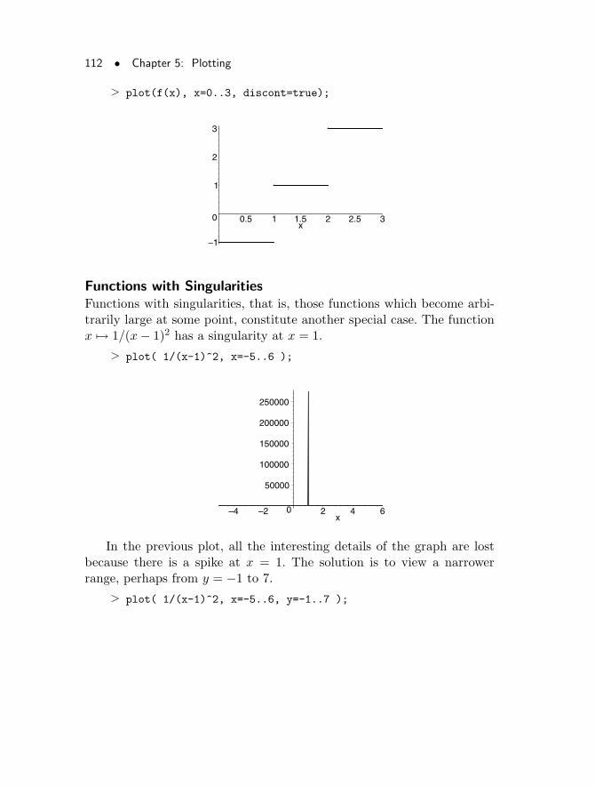
112 • Chapter 5: Plotting
> plot(f(x), x=0..3, discont=true);
–1
0
1
2
3
0.5 1 1.5 2 2.5 3x
Functions with SingularitiesFunctions with singularities, that is, those functions which become arbi-trarily large at some point, constitute another special case. The functionx 7→ 1/(x− 1)2 has a singularity at x = 1.
> plot( 1/(x-1)^2, x=-5..6 );
0
50000
100000
150000
200000
250000
–4 –2 2 4 6x
In the previous plot, all the interesting details of the graph are lostbecause there is a spike at x = 1. The solution is to view a narrowerrange, perhaps from y = −1 to 7.
> plot( 1/(x-1)^2, x=-5..6, y=-1..7 );
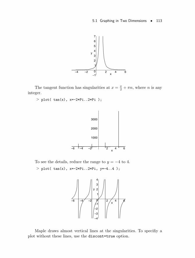
5.1 Graphing in Two Dimensions • 113
–10
1
2
3
4
5
6
7
y
–4 –2 2 4 6x
The tangent function has singularities at x = π2 + πn, where n is any
integer.
> plot( tan(x), x=-2*Pi..2*Pi );
1000
2000
3000
–6 –4 –2 2 4 6x
To see the details, reduce the range to y = −4 to 4.
> plot( tan(x), x=-2*Pi..2*Pi, y=-4..4 );
–4
–3
–2
–10
1
2
3
4
y
–6 –4 –2 2 4 6x
Maple draws almost vertical lines at the singularities. To specifiy aplot without these lines, use the discont=true option.
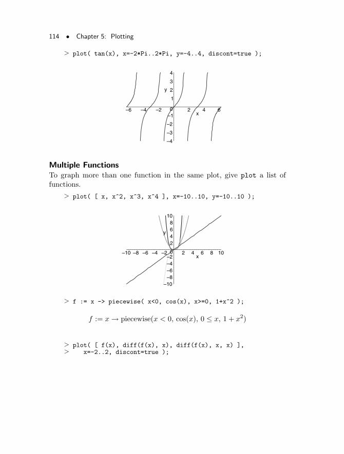
114 • Chapter 5: Plotting
> plot( tan(x), x=-2*Pi..2*Pi, y=-4..4, discont=true );
–4
–3
–2
–10
1
2
3
4
y
–6 –4 –2 2 4 6x
Multiple FunctionsTo graph more than one function in the same plot, give plot a list offunctions.
> plot( [ x, x^2, x^3, x^4 ], x=-10..10, y=-10..10 );
–10–8–6–4–2
0
2468
10
y
–10 –8 –6 –4 –2 2 4 6 8 10x
> f := x -> piecewise( x<0, cos(x), x>=0, 1+x^2 );
f := x → piecewise(x < 0, cos(x), 0 ≤ x, 1 + x2)
> plot( [ f(x), diff(f(x), x), diff(f(x), x, x) ],> x=-2..2, discont=true );
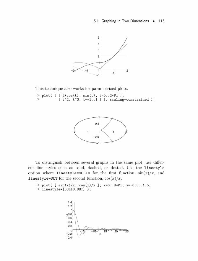
5.1 Graphing in Two Dimensions • 115
–1
0
1
2
3
4
5
–2 –1 1 2x
This technique also works for parametrized plots.
> plot( [ [ 2*cos(t), sin(t), t=0..2*Pi ],> [ t^2, t^3, t=-1..1 ] ], scaling=constrained );
–1
–0.5
0.5
1
–2 –1 1 2
To distinguish between several graphs in the same plot, use differ-ent line styles such as solid, dashed, or dotted. Use the linestyle
option where linestyle=SOLID for the first function, sin(x)/x, andlinestyle=DOT for the second function, cos(x)/x.
> plot( [ sin(x)/x, cos(x)/x ], x=0..8*Pi, y=-0.5..1.5,> linestyle=[SOLID,DOT] );
–0.4–0.2
0
0.20.40.60.8
11.21.4
y
5 10 15 20 25x
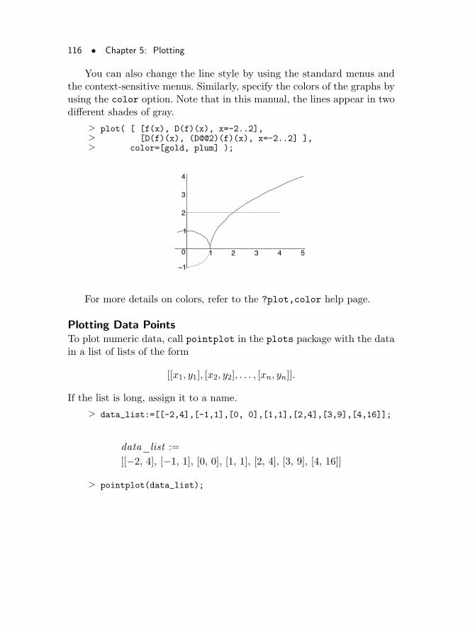
116 • Chapter 5: Plotting
You can also change the line style by using the standard menus andthe context-sensitive menus. Similarly, specify the colors of the graphs byusing the color option. Note that in this manual, the lines appear in twodifferent shades of gray.
> plot( [ [f(x), D(f)(x), x=-2..2],> [D(f)(x), (D@@2)(f)(x), x=-2..2] ],> color=[gold, plum] );
–1
0
1
2
3
4
1 2 3 4 5
For more details on colors, refer to the ?plot,color help page.
Plotting Data PointsTo plot numeric data, call pointplot in the plots package with the datain a list of lists of the form
[[x1, y1], [x2, y2], . . . , [xn, yn]].
If the list is long, assign it to a name.
> data_list:=[[-2,4],[-1,1],[0, 0],[1,1],[2,4],[3,9],[4,16]];
data_list :=
[[−2, 4], [−1, 1], [0, 0], [1, 1], [2, 4], [3, 9], [4, 16]]
> pointplot(data_list);
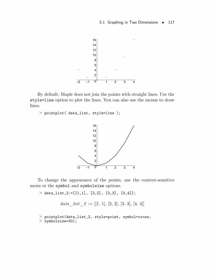
5.1 Graphing in Two Dimensions • 117
0
2
4
6
8
10
12
14
16
–2 –1 1 2 3 4
By default, Maple does not join the points with straight lines. Use thestyle=line option to plot the lines. You can also use the menus to drawlines.
> pointplot( data_list, style=line );
0
2
4
6
8
10
12
14
16
–2 –1 1 2 3 4
To change the appearance of the points, use the context-sensitivemenu or the symbol and symbolsize options.
> data_list_2:=[[1,1], [2,2], [3,3], [4,4]];
data_list_2 := [[1, 1], [2, 2], [3, 3], [4, 4]]
> pointplot(data_list_2, style=point, symbol=cross,> symbolsize=30);
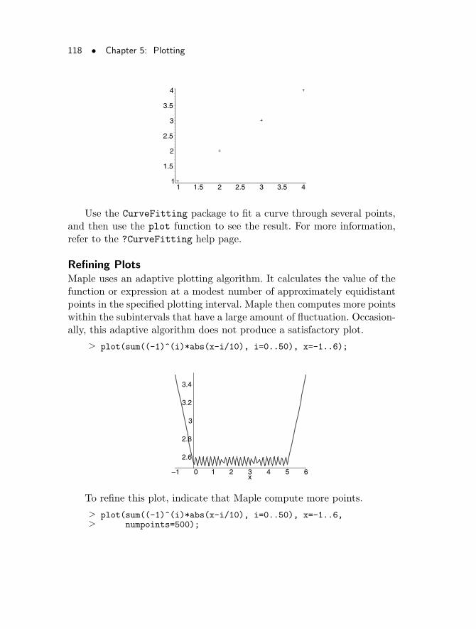
118 • Chapter 5: Plotting
1
1.5
2
2.5
3
3.5
4
1 1.5 2 2.5 3 3.5 4
Use the CurveFitting package to fit a curve through several points,and then use the plot function to see the result. For more information,refer to the ?CurveFitting help page.
Refining PlotsMaple uses an adaptive plotting algorithm. It calculates the value of thefunction or expression at a modest number of approximately equidistantpoints in the specified plotting interval. Maple then computes more pointswithin the subintervals that have a large amount of fluctuation. Occasion-ally, this adaptive algorithm does not produce a satisfactory plot.
> plot(sum((-1)^(i)*abs(x-i/10), i=0..50), x=-1..6);
2.6
2.8
3
3.2
3.4
–1 0 1 2 3 4 5 6x
To refine this plot, indicate that Maple compute more points.
> plot(sum((-1)^(i)*abs(x-i/10), i=0..50), x=-1..6,> numpoints=500);
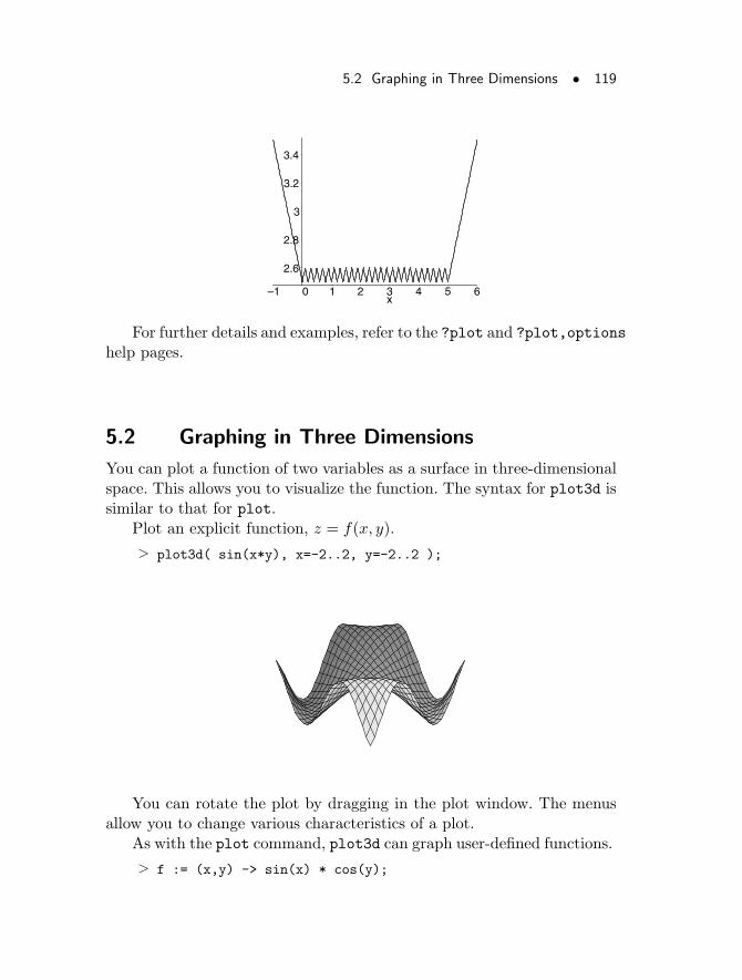
5.2 Graphing in Three Dimensions • 119
2.6
2.8
3
3.2
3.4
–1 0 1 2 3 4 5 6x
For further details and examples, refer to the ?plot and ?plot,options
help pages.
5.2 Graphing in Three Dimensions
You can plot a function of two variables as a surface in three-dimensionalspace. This allows you to visualize the function. The syntax for plot3d issimilar to that for plot.
Plot an explicit function, z = f(x, y).
> plot3d( sin(x*y), x=-2..2, y=-2..2 );
You can rotate the plot by dragging in the plot window. The menusallow you to change various characteristics of a plot.
As with the plot command, plot3d can graph user-defined functions.
> f := (x,y) -> sin(x) * cos(y);
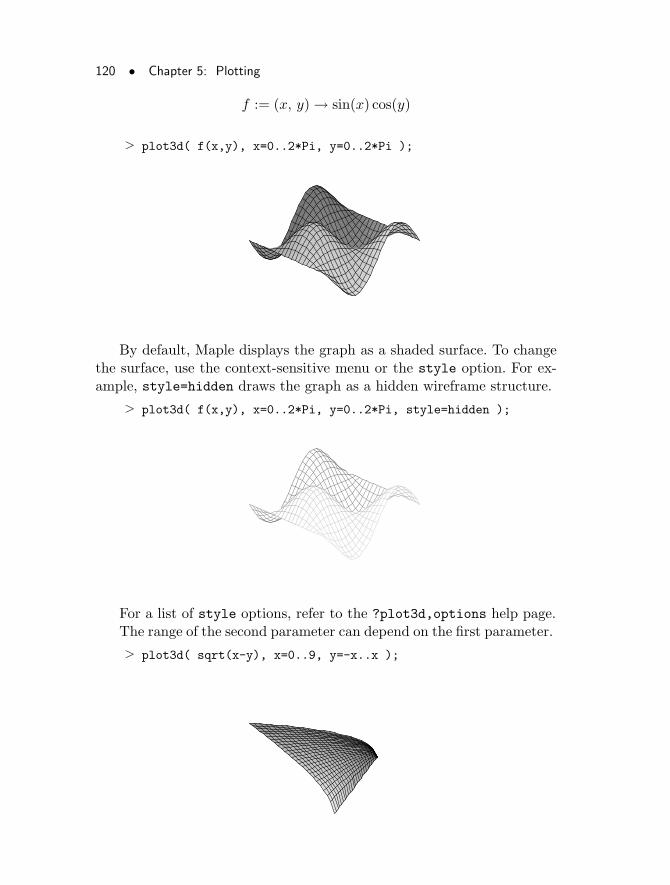
120 • Chapter 5: Plotting
f := (x, y) → sin(x) cos(y)
> plot3d( f(x,y), x=0..2*Pi, y=0..2*Pi );
By default, Maple displays the graph as a shaded surface. To changethe surface, use the context-sensitive menu or the style option. For ex-ample, style=hidden draws the graph as a hidden wireframe structure.
> plot3d( f(x,y), x=0..2*Pi, y=0..2*Pi, style=hidden );
For a list of style options, refer to the ?plot3d,options help page.The range of the second parameter can depend on the first parameter.
> plot3d( sqrt(x-y), x=0..9, y=-x..x );
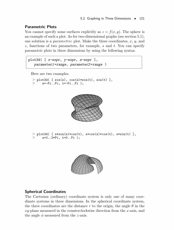
5.2 Graphing in Three Dimensions • 121
Parametric PlotsYou cannot specify some surfaces explicitly as z = f(x, y). The sphere isan example of such a plot. As for two-dimensional graphs (see section 5.1),one solution is a parametric plot. Make the three coordinates, x, y, andz, functions of two parameters, for example, s and t. You can specifyparametric plots in three dimensions by using the following syntax.
plot3d( [ x-expr, y-expr, z-expr ],
parameter1=range, parameter2=range )
Here are two examples.
> plot3d( [ sin(s), cos(s)*sin(t), sin(t) ],> s=-Pi..Pi, t=-Pi..Pi );
> plot3d( [ s*sin(s)*cos(t), s*cos(s)*cos(t), s*sin(t) ],> s=0..2*Pi, t=0..Pi );
Spherical CoordinatesThe Cartesian (ordinary) coordinate system is only one of many coor-dinate systems in three dimensions. In the spherical coordinate system,the three coordinates are the distance r to the origin, the angle θ in thexy-plane measured in the counterclockwise direction from the x-axis, andthe angle φ measured from the z-axis.
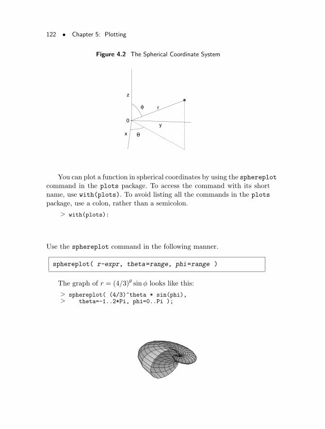
122 • Chapter 5: Plotting
Figure 4.2 The Spherical Coordinate System
θ
rφ
0
z
y
x
You can plot a function in spherical coordinates by using the sphereplotcommand in the plots package. To access the command with its shortname, use with(plots). To avoid listing all the commands in the plots
package, use a colon, rather than a semicolon.
> with(plots):
Use the sphereplot command in the following manner.
sphereplot( r-expr, theta=range, phi=range )
The graph of r = (4/3)θ sinφ looks like this:
> sphereplot( (4/3)^theta * sin(phi),> theta=-1..2*Pi, phi=0..Pi );
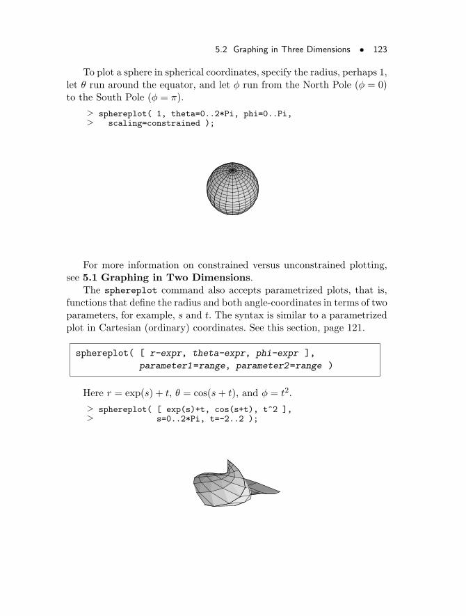
5.2 Graphing in Three Dimensions • 123
To plot a sphere in spherical coordinates, specify the radius, perhaps 1,let θ run around the equator, and let φ run from the North Pole (φ = 0)to the South Pole (φ = π).
> sphereplot( 1, theta=0..2*Pi, phi=0..Pi,> scaling=constrained );
For more information on constrained versus unconstrained plotting,see 5.1 Graphing in Two Dimensions.
The sphereplot command also accepts parametrized plots, that is,functions that define the radius and both angle-coordinates in terms of twoparameters, for example, s and t. The syntax is similar to a parametrizedplot in Cartesian (ordinary) coordinates. See this section, page 121.
sphereplot( [ r-expr, theta-expr, phi-expr ],
parameter1=range, parameter2=range )
Here r = exp(s) + t, θ = cos(s+ t), and φ = t2.
> sphereplot( [ exp(s)+t, cos(s+t), t^2 ],> s=0..2*Pi, t=-2..2 );
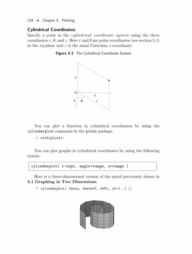
124 • Chapter 5: Plotting
Cylindrical CoordinatesSpecify a point in the cylindrical coordinate system using the threecoordinates r, θ, and z. Here r and θ are polar coordinates (see section 5.1)in the xy-plane and z is the usual Cartesian z-coordinate.
Figure 4.3 The Cylindrical Coordinate System
rθ
0
z
y
x
You can plot a function in cylindrical coordinates by using thecylinderplot command in the plots package.
> with(plots):
You can plot graphs in cylindrical coordinates by using the followingsyntax.
cylinderplot( r-expr, angle=range, z=range )
Here is a three-dimensional version of the spiral previously shown in5.1 Graphing in Two Dimensions.
> cylinderplot( theta, theta=0..4*Pi, z=-1..1 );
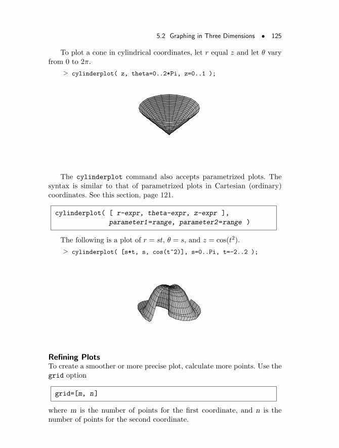
5.2 Graphing in Three Dimensions • 125
To plot a cone in cylindrical coordinates, let r equal z and let θ varyfrom 0 to 2π.
> cylinderplot( z, theta=0..2*Pi, z=0..1 );
The cylinderplot command also accepts parametrized plots. Thesyntax is similar to that of parametrized plots in Cartesian (ordinary)coordinates. See this section, page 121.
cylinderplot( [ r-expr, theta-expr, z-expr ],
parameter1=range, parameter2=range )
The following is a plot of r = st, θ = s, and z = cos(t2).
> cylinderplot( [s*t, s, cos(t^2)], s=0..Pi, t=-2..2 );
Refining PlotsTo create a smoother or more precise plot, calculate more points. Use thegrid option
grid=[m, n]
where m is the number of points for the first coordinate, and n is thenumber of points for the second coordinate.
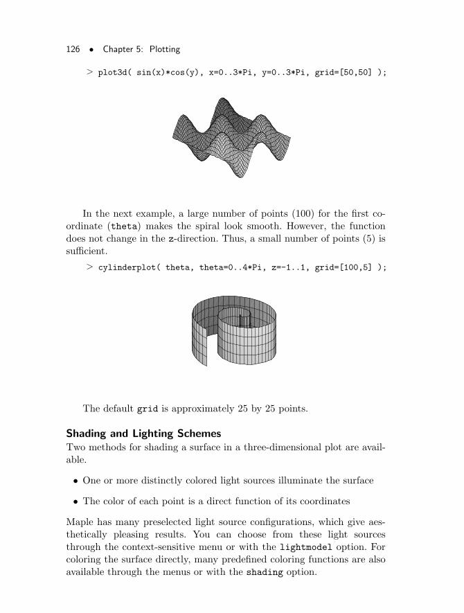
126 • Chapter 5: Plotting
> plot3d( sin(x)*cos(y), x=0..3*Pi, y=0..3*Pi, grid=[50,50] );
In the next example, a large number of points (100) for the first co-ordinate (theta) makes the spiral look smooth. However, the functiondoes not change in the z-direction. Thus, a small number of points (5) issufficient.
> cylinderplot( theta, theta=0..4*Pi, z=-1..1, grid=[100,5] );
The default grid is approximately 25 by 25 points.
Shading and Lighting SchemesTwo methods for shading a surface in a three-dimensional plot are avail-able.
• One or more distinctly colored light sources illuminate the surface
• The color of each point is a direct function of its coordinates
Maple has many preselected light source configurations, which give aes-thetically pleasing results. You can choose from these light sourcesthrough the context-sensitive menu or with the lightmodel option. Forcoloring the surface directly, many predefined coloring functions are alsoavailable through the menus or with the shading option.
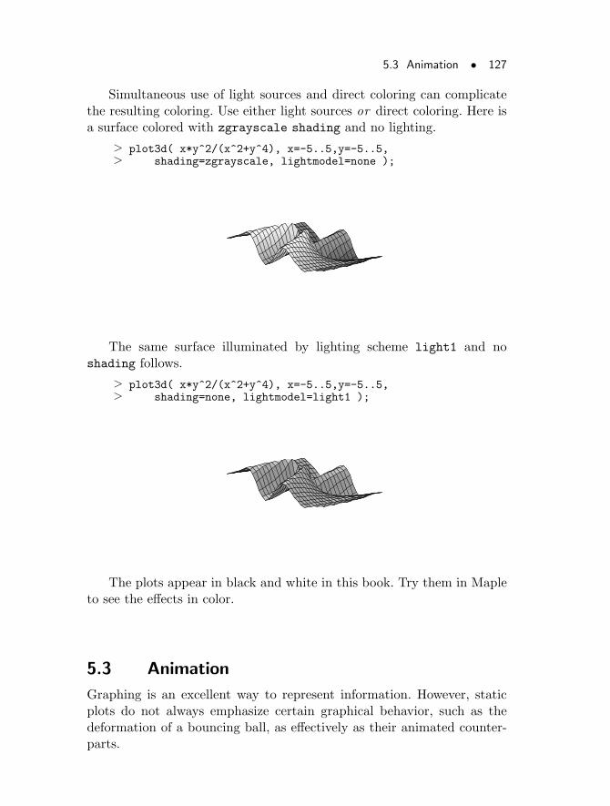
5.3 Animation • 127
Simultaneous use of light sources and direct coloring can complicatethe resulting coloring. Use either light sources or direct coloring. Here isa surface colored with zgrayscale shading and no lighting.
> plot3d( x*y^2/(x^2+y^4), x=-5..5,y=-5..5,> shading=zgrayscale, lightmodel=none );
The same surface illuminated by lighting scheme light1 and noshading follows.
> plot3d( x*y^2/(x^2+y^4), x=-5..5,y=-5..5,> shading=none, lightmodel=light1 );
The plots appear in black and white in this book. Try them in Mapleto see the effects in color.
5.3 Animation
Graphing is an excellent way to represent information. However, staticplots do not always emphasize certain graphical behavior, such as thedeformation of a bouncing ball, as effectively as their animated counter-parts.
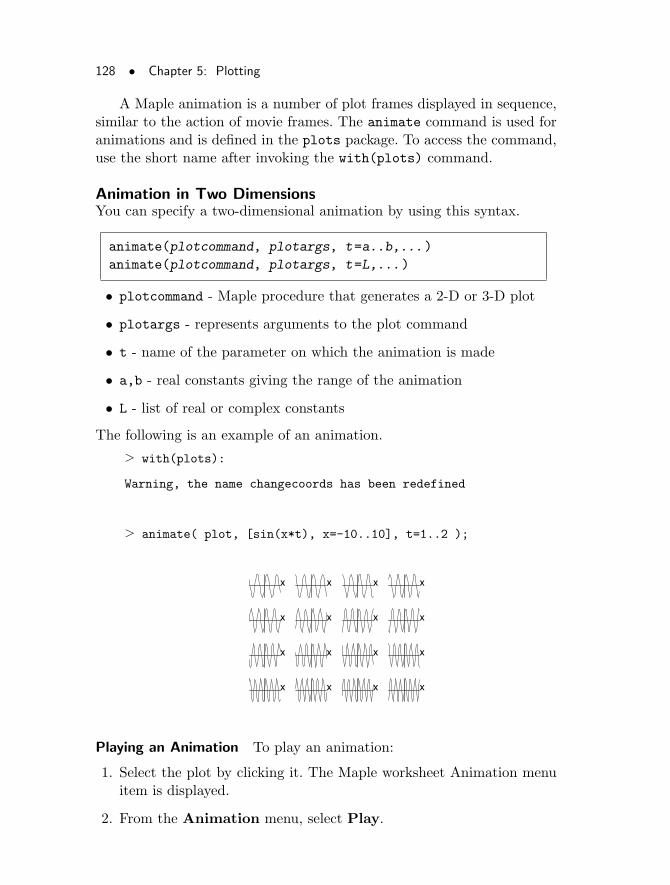
128 • Chapter 5: Plotting
A Maple animation is a number of plot frames displayed in sequence,similar to the action of movie frames. The animate command is used foranimations and is defined in the plots package. To access the command,use the short name after invoking the with(plots) command.
Animation in Two DimensionsYou can specify a two-dimensional animation by using this syntax.
animate(plotcommand, plotargs, t=a..b,...)
animate(plotcommand, plotargs, t=L,...)
• plotcommand - Maple procedure that generates a 2-D or 3-D plot
• plotargs - represents arguments to the plot command
• t - name of the parameter on which the animation is made
• a,b - real constants giving the range of the animation
• L - list of real or complex constants
The following is an example of an animation.
> with(plots):
Warning, the name changecoords has been redefined
> animate( plot, [sin(x*t), x=-10..10], t=1..2 );
xxxx
xxxx
xxxx
xxxx
Playing an Animation To play an animation:
1. Select the plot by clicking it. The Maple worksheet Animation menuitem is displayed.
2. From the Animation menu, select Play.
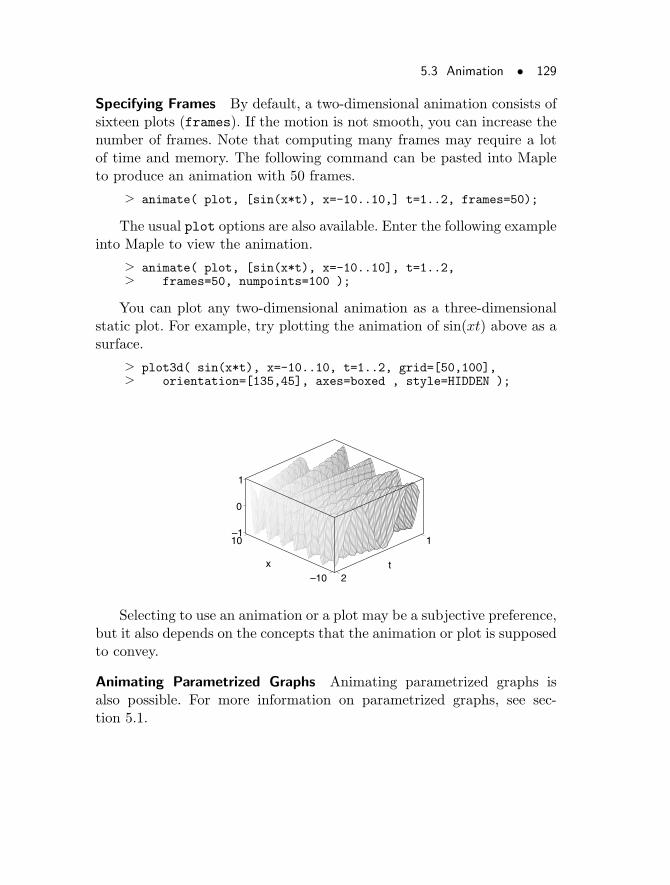
5.3 Animation • 129
Specifying Frames By default, a two-dimensional animation consists ofsixteen plots (frames). If the motion is not smooth, you can increase thenumber of frames. Note that computing many frames may require a lotof time and memory. The following command can be pasted into Mapleto produce an animation with 50 frames.
> animate( plot, [sin(x*t), x=-10..10,] t=1..2, frames=50);
The usual plot options are also available. Enter the following exampleinto Maple to view the animation.
> animate( plot, [sin(x*t), x=-10..10], t=1..2,> frames=50, numpoints=100 );
You can plot any two-dimensional animation as a three-dimensionalstatic plot. For example, try plotting the animation of sin(xt) above as asurface.
> plot3d( sin(x*t), x=-10..10, t=1..2, grid=[50,100],> orientation=[135,45], axes=boxed , style=HIDDEN );
–10
10
x
1
2t
–1
0
1
Selecting to use an animation or a plot may be a subjective preference,but it also depends on the concepts that the animation or plot is supposedto convey.
Animating Parametrized Graphs Animating parametrized graphs isalso possible. For more information on parametrized graphs, see sec-tion 5.1.
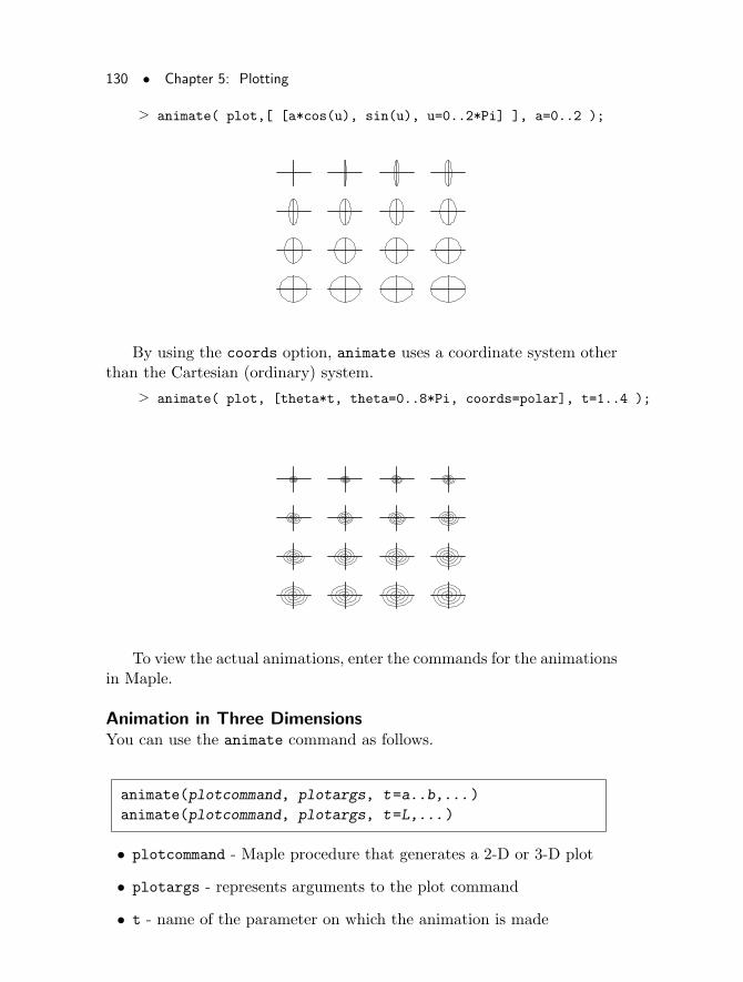
130 • Chapter 5: Plotting
> animate( plot,[ [a*cos(u), sin(u), u=0..2*Pi] ], a=0..2 );
By using the coords option, animate uses a coordinate system otherthan the Cartesian (ordinary) system.
> animate( plot, [theta*t, theta=0..8*Pi, coords=polar], t=1..4 );
To view the actual animations, enter the commands for the animationsin Maple.
Animation in Three DimensionsYou can use the animate command as follows.
animate(plotcommand, plotargs, t=a..b,...)
animate(plotcommand, plotargs, t=L,...)
• plotcommand - Maple procedure that generates a 2-D or 3-D plot
• plotargs - represents arguments to the plot command
• t - name of the parameter on which the animation is made
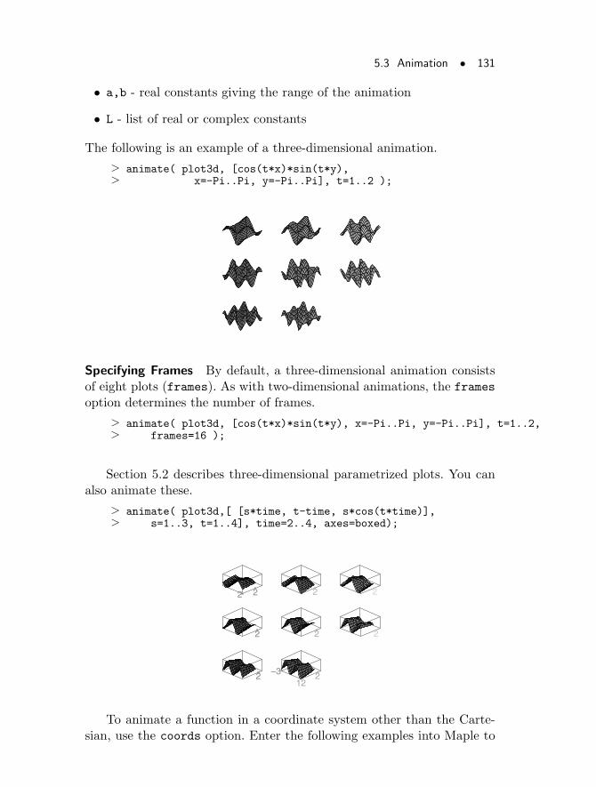
5.3 Animation • 131
• a,b - real constants giving the range of the animation
• L - list of real or complex constants
The following is an example of a three-dimensional animation.
> animate( plot3d, [cos(t*x)*sin(t*y),> x=-Pi..Pi, y=-Pi..Pi], t=1..2 );
Specifying Frames By default, a three-dimensional animation consistsof eight plots (frames). As with two-dimensional animations, the framesoption determines the number of frames.
> animate( plot3d, [cos(t*x)*sin(t*y), x=-Pi..Pi, y=-Pi..Pi], t=1..2,> frames=16 );
Section 5.2 describes three-dimensional parametrized plots. You canalso animate these.
> animate( plot3d,[ [s*time, t-time, s*cos(t*time)],> s=1..3, t=1..4], time=2..4, axes=boxed);
122 2–3
2 2 2
2 2 2 2
To animate a function in a coordinate system other than the Carte-sian, use the coords option. Enter the following examples into Maple to
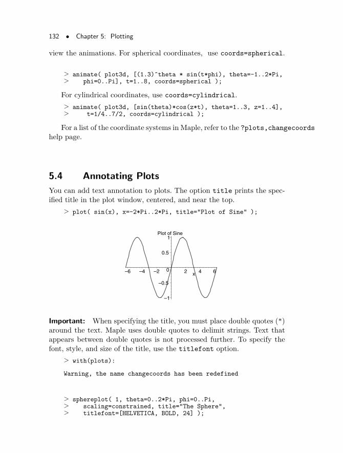
132 • Chapter 5: Plotting
view the animations. For spherical coordinates, use coords=spherical.
> animate( plot3d, [(1.3)^theta * sin(t*phi), theta=-1..2*Pi,> phi=0..Pi], t=1..8, coords=spherical );
For cylindrical coordinates, use coords=cylindrical.
> animate( plot3d, [sin(theta)*cos(z*t), theta=1..3, z=1..4],> t=1/4..7/2, coords=cylindrical );
For a list of the coordinate systems in Maple, refer to the ?plots,changecoordshelp page.
5.4 Annotating Plots
You can add text annotation to plots. The option title prints the spec-ified title in the plot window, centered, and near the top.
> plot( sin(x), x=-2*Pi..2*Pi, title="Plot of Sine" );
Plot of Sine
–1
–0.5
0
0.5
1
–6 –4 –2 2 4 6x
Important: When specifying the title, you must place double quotes (")around the text. Maple uses double quotes to delimit strings. Text thatappears between double quotes is not processed further. To specify thefont, style, and size of the title, use the titlefont option.
> with(plots):
Warning, the name changecoords has been redefined
> sphereplot( 1, theta=0..2*Pi, phi=0..Pi,> scaling=constrained, title="The Sphere",> titlefont=[HELVETICA, BOLD, 24] );
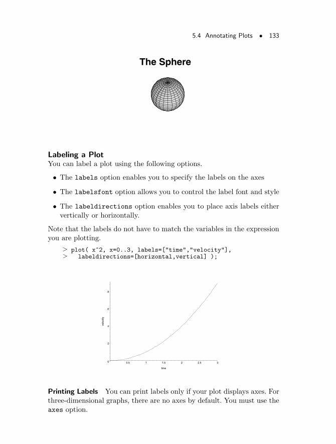
5.4 Annotating Plots • 133
The Sphere
Labeling a PlotYou can label a plot using the following options.
• The labels option enables you to specify the labels on the axes
• The labelsfont option allows you to control the label font and style
• The labeldirections option enables you to place axis labels eithervertically or horizontally.
Note that the labels do not have to match the variables in the expressionyou are plotting.
> plot( x^2, x=0..3, labels=["time","velocity"],> labeldirections=[horizontal,vertical] );
0
2
4
6
8
velo
city
0.5 1 1.5 2 2.5 3
time
Printing Labels You can print labels only if your plot displays axes. Forthree-dimensional graphs, there are no axes by default. You must use theaxes option.
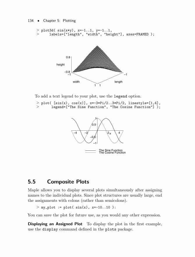
134 • Chapter 5: Plotting
> plot3d( sin(x*y), x=-1..1, y=-1..1,> labels=["length", "width", "height"], axes=FRAMED );
–1
1length
–1
1width
–0.8
0.8
height
To add a text legend to your plot, use the legend option.
> plot( [sin(x), cos(x)], x=-3*Pi/2..3*Pi/2, linestyle=[1,4],> legend=["The Sine Function", "The Cosine Function"] );
The Sine FunctionThe Cosine Function
–1
–0.5
0.5
1
–4 –2 2 4x
5.5 Composite Plots
Maple allows you to display several plots simultaneously after assigningnames to the individual plots. Since plot structures are usually large, endthe assignments with colons (rather than semicolons).
> my_plot := plot( sin(x), x=-10..10 ):
You can save the plot for future use, as you would any other expression.
Displaying an Assigned Plot To display the plot in the first example,use the display command defined in the plots package.
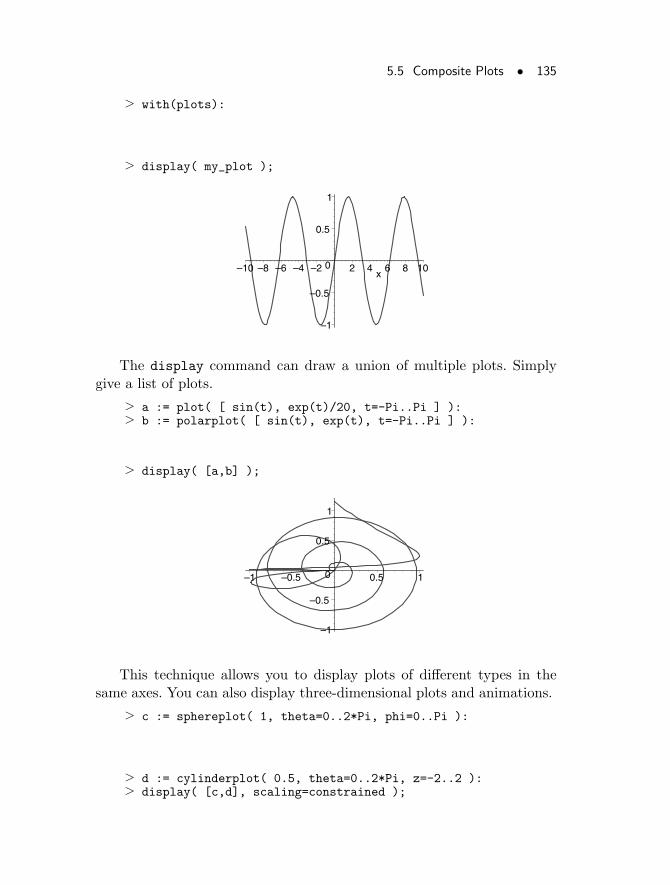
5.5 Composite Plots • 135
> with(plots):
> display( my_plot );
–1
–0.5
0
0.5
1
–10 –8 –6 –4 –2 2 4 6 8 10x
The display command can draw a union of multiple plots. Simplygive a list of plots.
> a := plot( [ sin(t), exp(t)/20, t=-Pi..Pi ] ):> b := polarplot( [ sin(t), exp(t), t=-Pi..Pi ] ):
> display( [a,b] );
–1
–0.5
0
0.5
1
–1 –0.5 0.5 1
This technique allows you to display plots of different types in thesame axes. You can also display three-dimensional plots and animations.
> c := sphereplot( 1, theta=0..2*Pi, phi=0..Pi ):
> d := cylinderplot( 0.5, theta=0..2*Pi, z=-2..2 ):> display( [c,d], scaling=constrained );
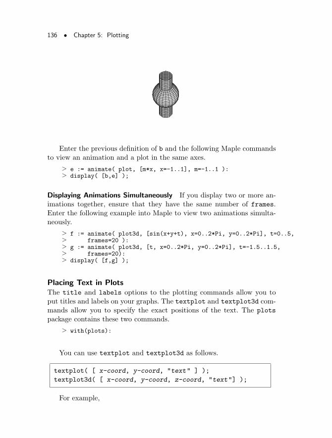
136 • Chapter 5: Plotting
Enter the previous definition of b and the following Maple commandsto view an animation and a plot in the same axes.
> e := animate( plot, [m*x, x=-1..1], m=-1..1 ):> display( [b,e] );
Displaying Animations Simultaneously If you display two or more an-imations together, ensure that they have the same number of frames.Enter the following example into Maple to view two animations simulta-neously.
> f := animate( plot3d, [sin(x+y+t), x=0..2*Pi, y=0..2*Pi], t=0..5,> frames=20 ):> g := animate( plot3d, [t, x=0..2*Pi, y=0..2*Pi], t=-1.5..1.5,> frames=20):> display( [f,g] );
Placing Text in PlotsThe title and labels options to the plotting commands allow you toput titles and labels on your graphs. The textplot and textplot3d com-mands allow you to specify the exact positions of the text. The plots
package contains these two commands.
> with(plots):
You can use textplot and textplot3d as follows.
textplot( [ x-coord, y-coord, "text" ] );
textplot3d( [ x-coord, y-coord, z-coord, "text"] );
For example,
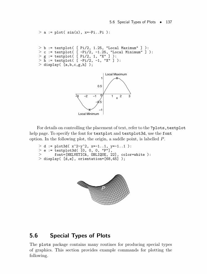
5.6 Special Types of Plots • 137
> a := plot( sin(x), x=-Pi..Pi ):
> b := textplot( [ Pi/2, 1.25, "Local Maximum" ] ):> c := textplot( [ -Pi/2, -1.25, "Local Minimum" ] ):> g := textplot( [ Pi/2, 1, "X" ] ):> h := textplot( [ -Pi/2, -1, "X" ] ):> display( [a,b,c,g,h] );
X
X
Local Minimum
Local Maximum
–1
–0.5
0
0.5
1
–3 –2 –1 1 2 3x
For details on controlling the placement of text, refer to the ?plots,textplothelp page. To specify the font for textplot and textplot3d, use the fontoption. In the following plot, the origin, a saddle point, is labelled P .
> d := plot3d( x^2-y^2, x=-1..1, y=-1..1 ):> e := textplot3d( [0, 0, 0, "P"],> font=[HELVETICA, OBLIQUE, 22], color=white ):> display( [d,e], orientation=[68,45] );
P
5.6 Special Types of Plots
The plots package contains many routines for producing special typesof graphics. This section provides example commands for plotting thefollowing.
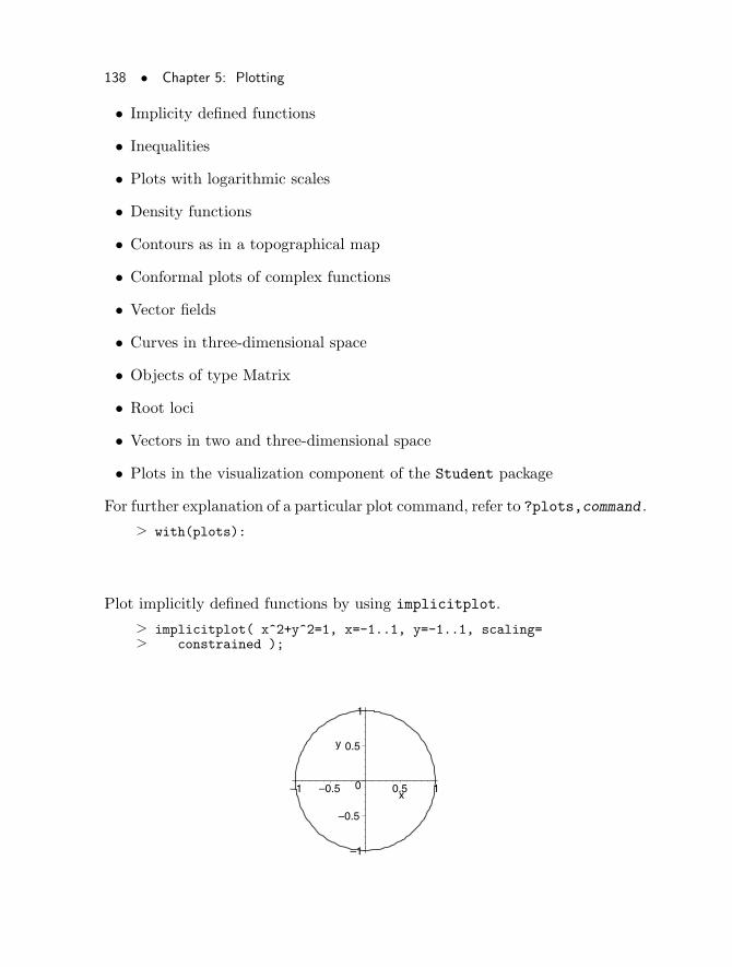
138 • Chapter 5: Plotting
• Implicity defined functions
• Inequalities
• Plots with logarithmic scales
• Density functions
• Contours as in a topographical map
• Conformal plots of complex functions
• Vector fields
• Curves in three-dimensional space
• Objects of type Matrix
• Root loci
• Vectors in two and three-dimensional space
• Plots in the visualization component of the Student package
For further explanation of a particular plot command, refer to ?plots,command .
> with(plots):
Plot implicitly defined functions by using implicitplot.
> implicitplot( x^2+y^2=1, x=-1..1, y=-1..1, scaling=> constrained );
–1
–0.5
0
0.5
1
y
–1 –0.5 0.5 1x
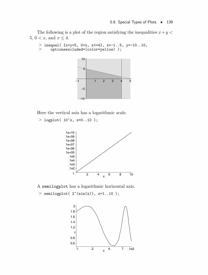
5.6 Special Types of Plots • 139
The following is a plot of the region satisfying the inequalities x+y <5, 0 < x, and x ≤ 4.
> inequal( {x+y<5, 0<x, x<=4}, x=-1..5, y=-10..10,> optionsexcluded=(color=yellow) );
–10
–5
5
10
–1 1 2 3 4 5
Here the vertical axis has a logarithmic scale.
> logplot( 10^x, x=0..10 );
1.
.1e2
.1e3
.1e4
.1e51e+051e+061e+071e+081e+091e+10
2 4 6 8 10x
A semilogplot has a logarithmic horizontal axis.
> semilogplot( 2^(sin(x)), x=1..10 );
0.6
0.8
1
1.2
1.4
1.6
1.8
2
1. 2. 4. 7. .1e2x
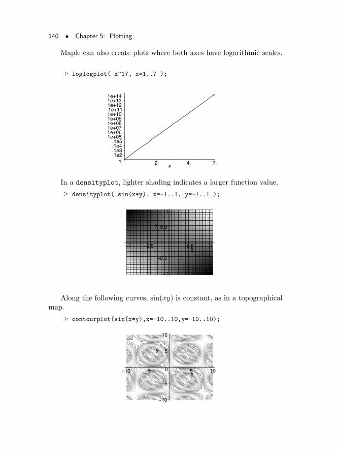
140 • Chapter 5: Plotting
Maple can also create plots where both axes have logarithmic scales.
> loglogplot( x^17, x=1..7 );
1..1e2.1e3.1e4.1e5
1e+051e+061e+071e+081e+091e+101e+111e+121e+131e+14
2. 4. 7.x
In a densityplot, lighter shading indicates a larger function value.
> densityplot( sin(x*y), x=-1..1, y=-1..1 );
–1
–0.5
0.5
1
y
–1 –0.5 0.5 1x
Along the following curves, sin(xy) is constant, as in a topographicalmap.
> contourplot(sin(x*y),x=-10..10,y=-10..10);
–10
–5
0
5
10
y
–10 –5 5 10x
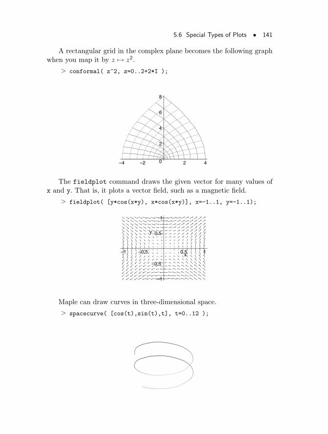
5.6 Special Types of Plots • 141
A rectangular grid in the complex plane becomes the following graphwhen you map it by z 7→ z2.
> conformal( z^2, z=0..2+2*I );
0
2
4
6
8
–4 –2 2 4
The fieldplot command draws the given vector for many values ofx and y. That is, it plots a vector field, such as a magnetic field.
> fieldplot( [y*cos(x*y), x*cos(x*y)], x=-1..1, y=-1..1);
–1
–0.5
0.5
1
y
–1 –0.5 0.5 1x
Maple can draw curves in three-dimensional space.
> spacecurve( [cos(t),sin(t),t], t=0..12 );
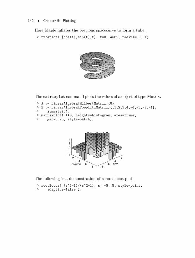
142 • Chapter 5: Plotting
Here Maple inflates the previous spacecurve to form a tube.
> tubeplot( [cos(t),sin(t),t], t=0..4*Pi, radius=0.5 );
The matrixplot command plots the values of a object of type Matrix.
> A := LinearAlgebra[HilbertMatrix](8):> B := LinearAlgebra[ToeplitzMatrix]([1,2,3,4,-4,-3,-2,-1],> symmetric):> matrixplot( A+B, heights=histogram, axes=frame,> gap=0.25, style=patch);
24
68
row
24
68
column
–4–2
024
The following is a demonstration of a root locus plot.
> rootlocus( (s^5-1)/(s^2+1), s, -5..5, style=point,> adaptive=false );
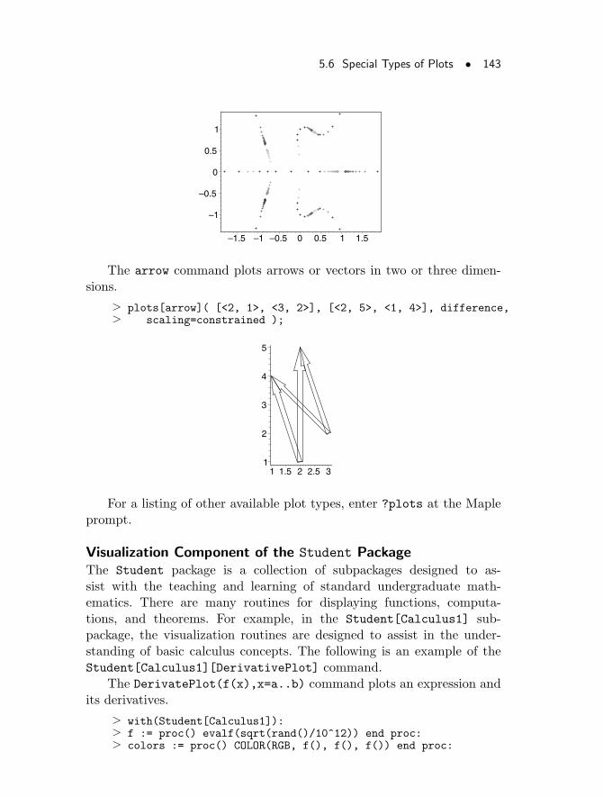
5.6 Special Types of Plots • 143
–1
–0.5
0
0.5
1
–1.5 –1 –0.5 0 0.5 1 1.5
The arrow command plots arrows or vectors in two or three dimen-sions.
> plots[arrow]( [<2, 1>, <3, 2>], [<2, 5>, <1, 4>], difference,> scaling=constrained );
1
2
3
4
5
1 1.5 2 2.5 3
For a listing of other available plot types, enter ?plots at the Mapleprompt.
Visualization Component of the Student PackageThe Student package is a collection of subpackages designed to as-sist with the teaching and learning of standard undergraduate math-ematics. There are many routines for displaying functions, computa-tions, and theorems. For example, in the Student[Calculus1] sub-package, the visualization routines are designed to assist in the under-standing of basic calculus concepts. The following is an example of theStudent[Calculus1][DerivativePlot] command.
The DerivatePlot(f(x),x=a..b) command plots an expression andits derivatives.
> with(Student[Calculus1]):> f := proc() evalf(sqrt(rand()/10^12)) end proc:> colors := proc() COLOR(RGB, f(), f(), f()) end proc:
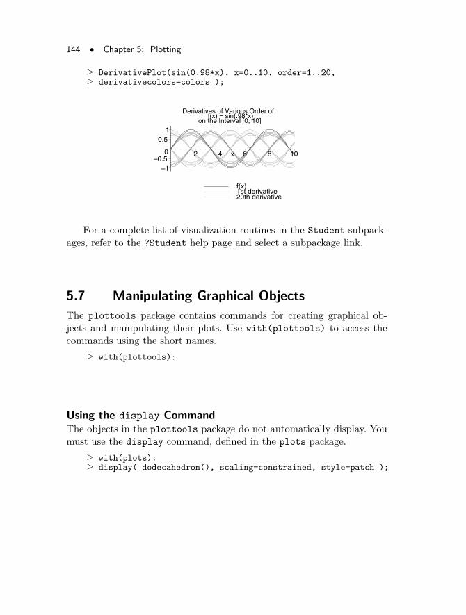
144 • Chapter 5: Plotting
> DerivativePlot(sin(0.98*x), x=0..10, order=1..20,> derivativecolors=colors );
f(x)1st derivative20th derivative
Derivatives of Various Order off(x) = sin(.98*x)
on the Interval [0, 10]
–1–0.5
0
0.51
2 4 6 8 10x
For a complete list of visualization routines in the Student subpack-ages, refer to the ?Student help page and select a subpackage link.
5.7 Manipulating Graphical Objects
The plottools package contains commands for creating graphical ob-jects and manipulating their plots. Use with(plottools) to access thecommands using the short names.
> with(plottools):
Using the display CommandThe objects in the plottools package do not automatically display. Youmust use the display command, defined in the plots package.
> with(plots):> display( dodecahedron(), scaling=constrained, style=patch );
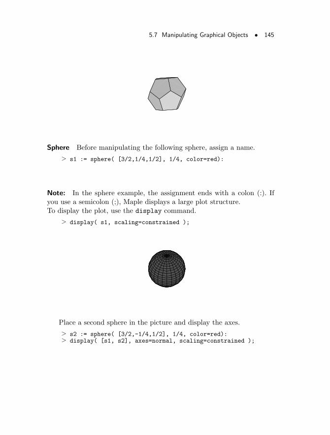
5.7 Manipulating Graphical Objects • 145
Sphere Before manipulating the following sphere, assign a name.
> s1 := sphere( [3/2,1/4,1/2], 1/4, color=red):
Note: In the sphere example, the assignment ends with a colon (:). Ifyou use a semicolon (;), Maple displays a large plot structure.To display the plot, use the display command.
> display( s1, scaling=constrained );
Place a second sphere in the picture and display the axes.
> s2 := sphere( [3/2,-1/4,1/2], 1/4, color=red):> display( [s1, s2], axes=normal, scaling=constrained );
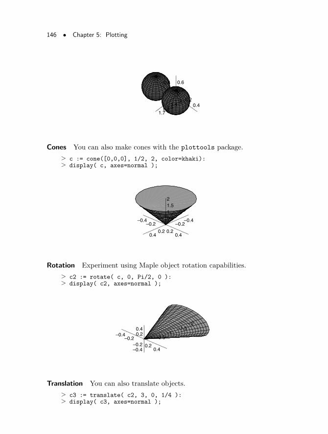
146 • Chapter 5: Plotting
0.4
0.6–0.4–0.2
00.2
0.41.3
1.41.5
1.61.7
Cones You can also make cones with the plottools package.
> c := cone([0,0,0], 1/2, 2, color=khaki):> display( c, axes=normal );
0.511.52
–0.4–0.2
0.20.4
–0.4–0.2
0.20.4
Rotation Experiment using Maple object rotation capabilities.
> c2 := rotate( c, 0, Pi/2, 0 ):> display( c2, axes=normal );
–0.4–0.2
0.20.4
–0.4–0.2
0.20.4
–2–1.5
–1–0.5
Translation You can also translate objects.
> c3 := translate( c2, 3, 0, 1/4 ):> display( c3, axes=normal );
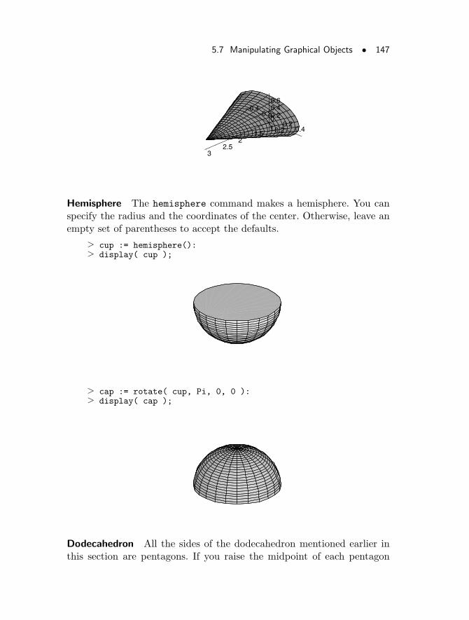
5.7 Manipulating Graphical Objects • 147
–0.2
0.20.40.6
–0.4–0.2
00.2
0.411.5
22.5
3
Hemisphere The hemisphere command makes a hemisphere. You canspecify the radius and the coordinates of the center. Otherwise, leave anempty set of parentheses to accept the defaults.
> cup := hemisphere():> display( cup );
> cap := rotate( cup, Pi, 0, 0 ):> display( cap );
Dodecahedron All the sides of the dodecahedron mentioned earlier inthis section are pentagons. If you raise the midpoint of each pentagon
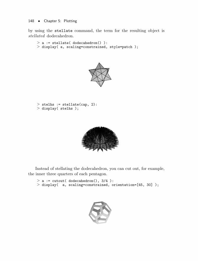
148 • Chapter 5: Plotting
by using the stellate command, the term for the resulting object isstellated dodecahedron.
> a := stellate( dodecahedron() ):> display( a, scaling=constrained, style=patch );
> stelhs := stellate(cap, 2):> display( stelhs );
Instead of stellating the dodecahedron, you can cut out, for example,the inner three quarters of each pentagon.
> a := cutout( dodecahedron(), 3/4 ):> display( a, scaling=constrained, orientation=[45, 30] );
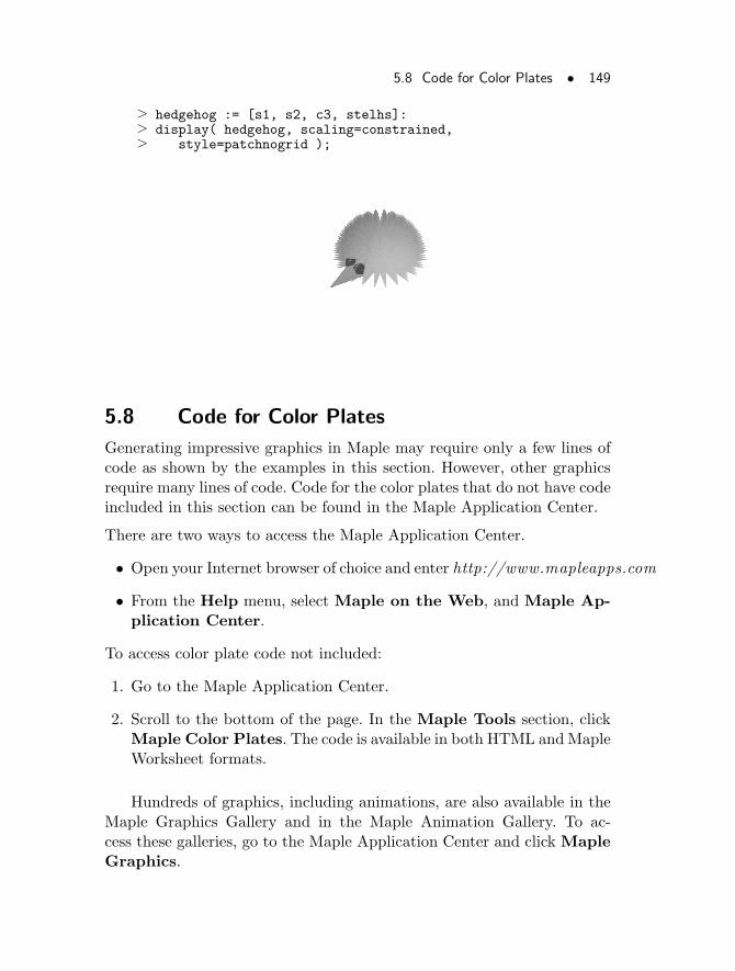
5.8 Code for Color Plates • 149
> hedgehog := [s1, s2, c3, stelhs]:> display( hedgehog, scaling=constrained,> style=patchnogrid );
5.8 Code for Color Plates
Generating impressive graphics in Maple may require only a few lines ofcode as shown by the examples in this section. However, other graphicsrequire many lines of code. Code for the color plates that do not have codeincluded in this section can be found in the Maple Application Center.
There are two ways to access the Maple Application Center.
• Open your Internet browser of choice and enter http://www.mapleapps.com
• From the Help menu, select Maple on the Web, and Maple Ap-plication Center.
To access color plate code not included:
1. Go to the Maple Application Center.
2. Scroll to the bottom of the page. In the Maple Tools section, clickMaple Color Plates. The code is available in both HTML and MapleWorksheet formats.
Hundreds of graphics, including animations, are also available in theMaple Graphics Gallery and in the Maple Animation Gallery. To ac-cess these galleries, go to the Maple Application Center and click MapleGraphics.
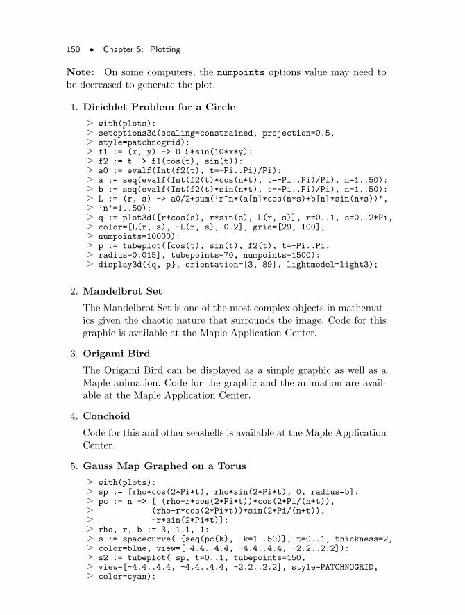
150 • Chapter 5: Plotting
Note: On some computers, the numpoints options value may need tobe decreased to generate the plot.
1. Dirichlet Problem for a Circle
> with(plots):> setoptions3d(scaling=constrained, projection=0.5,> style=patchnogrid):> f1 := (x, y) -> 0.5*sin(10*x*y):> f2 := t -> f1(cos(t), sin(t)):> a0 := evalf(Int(f2(t), t=-Pi..Pi)/Pi):> a := seq(evalf(Int(f2(t)*cos(n*t), t=-Pi..Pi)/Pi), n=1..50):> b := seq(evalf(Int(f2(t)*sin(n*t), t=-Pi..Pi)/Pi), n=1..50):> L := (r, s) -> a0/2+sum(’r^n*(a[n]*cos(n*s)+b[n]*sin(n*s))’,> ’n’=1..50):> q := plot3d([r*cos(s), r*sin(s), L(r, s)], r=0..1, s=0..2*Pi,> color=[L(r, s), -L(r, s), 0.2], grid=[29, 100],> numpoints=10000):> p := tubeplot([cos(t), sin(t), f2(t), t=-Pi..Pi,> radius=0.015], tubepoints=70, numpoints=1500):> display3d({q, p}, orientation=[3, 89], lightmodel=light3);
2. Mandelbrot Set
The Mandelbrot Set is one of the most complex objects in mathemat-ics given the chaotic nature that surrounds the image. Code for thisgraphic is available at the Maple Application Center.
3. Origami Bird
The Origami Bird can be displayed as a simple graphic as well as aMaple animation. Code for the graphic and the animation are avail-able at the Maple Application Center.
4. Conchoid
Code for this and other seashells is available at the Maple ApplicationCenter.
5. Gauss Map Graphed on a Torus
> with(plots):> sp := [rho*cos(2*Pi*t), rho*sin(2*Pi*t), 0, radius=b]:> pc := n -> [ (rho-r*cos(2*Pi*t))*cos(2*Pi/(n+t)),> (rho-r*cos(2*Pi*t))*sin(2*Pi/(n+t)),> -r*sin(2*Pi*t)]:> rho, r, b := 3, 1.1, 1:> s := spacecurve( {seq(pc(k), k=1..50)}, t=0..1, thickness=2,> color=blue, view=[-4.4..4.4, -4.4..4.4, -2.2..2.2]):> s2 := tubeplot( sp, t=0..1, tubepoints=150,> view=[-4.4..4.4, -4.4..4.4, -2.2..2.2], style=PATCHNOGRID,> color=cyan):
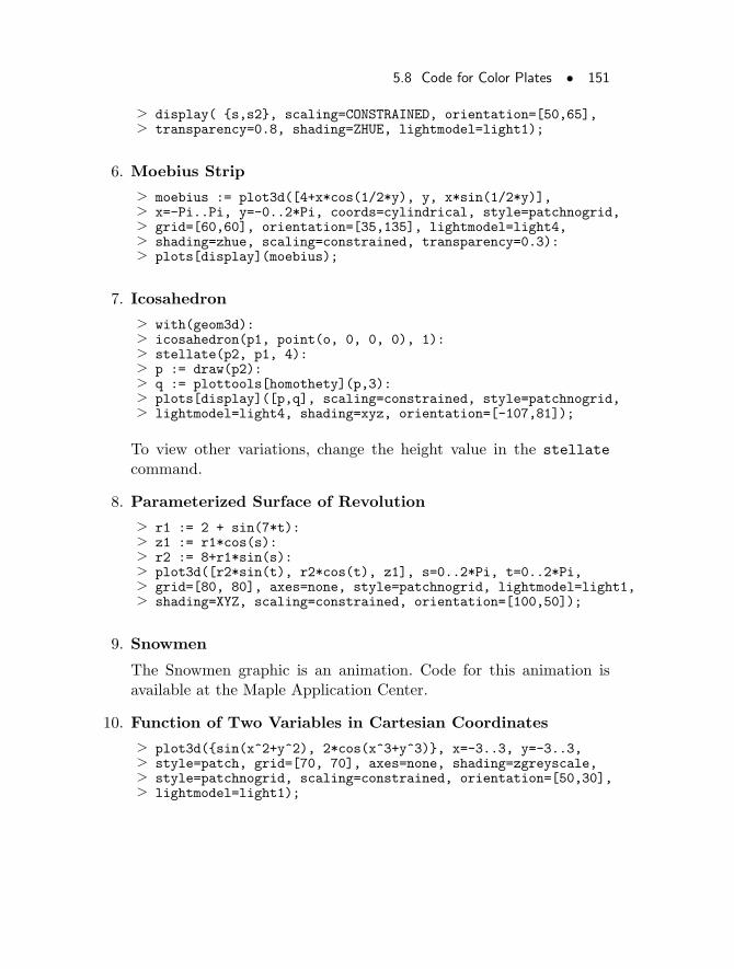
5.8 Code for Color Plates • 151
> display( {s,s2}, scaling=CONSTRAINED, orientation=[50,65],> transparency=0.8, shading=ZHUE, lightmodel=light1);
6. Moebius Strip
> moebius := plot3d([4+x*cos(1/2*y), y, x*sin(1/2*y)],> x=-Pi..Pi, y=-0..2*Pi, coords=cylindrical, style=patchnogrid,> grid=[60,60], orientation=[35,135], lightmodel=light4,> shading=zhue, scaling=constrained, transparency=0.3):> plots[display](moebius);
7. Icosahedron
> with(geom3d):> icosahedron(p1, point(o, 0, 0, 0), 1):> stellate(p2, p1, 4):> p := draw(p2):> q := plottools[homothety](p,3):> plots[display]([p,q], scaling=constrained, style=patchnogrid,> lightmodel=light4, shading=xyz, orientation=[-107,81]);
To view other variations, change the height value in the stellate
command.
8. Parameterized Surface of Revolution
> r1 := 2 + sin(7*t):> z1 := r1*cos(s):> r2 := 8+r1*sin(s):> plot3d([r2*sin(t), r2*cos(t), z1], s=0..2*Pi, t=0..2*Pi,> grid=[80, 80], axes=none, style=patchnogrid, lightmodel=light1,> shading=XYZ, scaling=constrained, orientation=[100,50]);
9. Snowmen
The Snowmen graphic is an animation. Code for this animation isavailable at the Maple Application Center.
10. Function of Two Variables in Cartesian Coordinates
> plot3d({sin(x^2+y^2), 2*cos(x^3+y^3)}, x=-3..3, y=-3..3,> style=patch, grid=[70, 70], axes=none, shading=zgreyscale,> style=patchnogrid, scaling=constrained, orientation=[50,30],> lightmodel=light1);
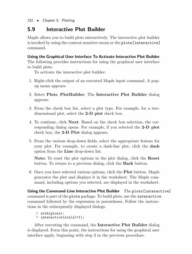
152 • Chapter 5: Plotting
5.9 Interactive Plot Builder
Maple allows you to build plots interactively. The interactive plot builderis invoked by using the context-sensitive menu or the plots[interactive]command.
Using the Graphical User Interface To Activate Interactive Plot BuilderThe following provides instructions for using the graphical user interfaceto build plots.
To activate the interactive plot builder:
1. Right-click the output of an executed Maple input command. A pop-up menu appears.
2. Select Plots, PlotBuilder. The Interactive Plot Builder dialogappears.
3. From the check box list, select a plot type. For example, for a two-dimensional plot, select the 2-D plot check box.
4. To continue, click Next. Based on the check box selection, the cor-responding dialog opens. For example, if you selected the 2-D plotcheck box, the 2-D Plot dialog appears.
5. From the various drop-down fields, select the appropriate feature foryour plot. For example, to create a dash-line plot, click the dashoption from the Line drop-down list.
Note: To reset the plot options in the plot dialog, click the Resetbutton. To return to a previous dialog, click the Back button.
6. Once you have selected various options, click the Plot button. Maplegenerates the plot and displays it in the worksheet. The Maple com-mand, including options you selected, are displayed in the worksheet.
Using the Command-Line Interactive Plot Builder The plots[interactive]command is part of the plots package. To build plots, use the interactivecommand followed by the expression in parentheses. Follow the instruc-tions in the subsequently displayed dialogs.
> with(plots):> interactive(sin(x)+1);
After executing the command, the Interactive Plot Builder dialogis displayed. Form this point, the instructions for using the graphical userinterface apply, beginning with step 3 in the previous procedure.
5.10 Conclusion • 153
5.10 Conclusion
This chapter examined Maple two- and three-dimensional plotting capa-bilities, involving explicitly, parametrically, and implicitly given functions.Cartesian, polar, spherical, and cylindrical are a few of the many coor-dinate systems that Maple can handle. Furthermore, you can animate agraph and shade it in a variety of ways for a clearer understanding of itsnature.
Use the commands found in the plots package to display variousgraphs of functions and expressions. Some of the special plot types thatyou can create using these commands include contour, density, and loga-rithmic plots. The commands within the plottools package create andmanipulate objects. Such commands, for instance, allow you to translate,rotate, and even stellate a graphical object. The interactive plot builderfacilitates specifying and displaying plots by providing a graphical userinterface.

154 • Chapter 5: Plotting
6 Evaluation andSimplification
Expression manipulation serves many purposes, for example, convertingoutput expressions into a familiar form to check answers or into a specificform needed by certain Maple routines. The issue of simplification is diffi-cult in symbolic mathematics. What is simple in one context may not bein another context—each individual context can have its own definitionof a simple form.
Working with Expressions in MapleMaple provides a set of tools for working with expressions, for performingboth mathematical and structural manipulations.
• Mathematical manipulations correspond to a standard mathematicalprocess, for example, factoring a polynomial, or rationalizing the de-nominator of a rational expression.
• Structural manipulation tools allow you to access and modify parts ofthe Maple data structures that represent expressions and other typesof objects.
In This Chapter• Mathematical manipulations
• Assumptions
• Structural manipulations
• Evaluation rules
155
156 • Chapter 6: Evaluation and Simplification
6.1 Mathematical Manipulations
Solving equations by hand usually involves performing a sequence of al-gebraic manipulations. You can also perform these steps using Maple.
> eq := 4*x + 17 = 23;
eq := 4x+ 17 = 23
To solve this equation, you must subtract 17 from both sides of theequation. Subtract the equation 17=17 from eq. Enclose the unnamedequation in parentheses.
> eq - ( 17 = 17 );
4x = 6
Divide through by 4. Note that you do not have to use 4=4 in thiscase.
> % / 4;
x =3
2
The following sections focus on more sophisticated manipulations.
Expanding Polynomials as SumsSums are generally easier to comprehend than products, so you may find ituseful to expand a polynomial as a sum of products. The expand commandhas this capability.
> poly := (x+1)*(x+2)*(x+5)*(x-3/2);
poly := (x+ 1) (x+ 2) (x+ 5) (x− 3
2)
> expand( poly );
x4 +13
2x3 + 5x2 − 31
2x− 15
The expand command expands the numerator of a rational expres-sion.
6.1 Mathematical Manipulations • 157
> expand( (x+1)*(y^2-2*y+1) / z / (y-1) );
x y2
z (y − 1)− 2
x y
z (y − 1)+
x
z (y − 1)+
y2
z (y − 1)− 2
y
z (y − 1)
+1
z (y − 1)
Note: To convert an expression containing fractions into a single rationalexpression and then cancel common factors, use the normal command. Seethis section, page 165.
Expansion Rules The expand command also recognizes expansion rulesfor many standard mathematical functions.
> expand( sin(2*x) );
2 sin(x) cos(x)
> ln( abs(x^2)/(1+abs(x)) );
ln(|x|2
1 + |x|)
> expand(%);
2 ln(|x|)− ln(1 + |x|)
The combine command recognizes the same rules but applies themin the opposite direction. For information on combining terms, see thissection, page 164.
You can specify subexpressions that you do not want to expand, asan argument to expand.
> expand( (x+1)*(y+z) );
x y + x z + y + z
> expand( (x+1)*(y+z), x+1 );
(x+ 1) y + (x+ 1) z
158 • Chapter 6: Evaluation and Simplification
You can expand an expression over a special domain.
> poly := (x+2)^2*(x-2)*(x+3)*(x-1)^2*(x-1);
poly := (x+ 2)2 (x− 2) (x+ 3) (x− 1)3
> expand( poly );
x7 + 2x6 − 10x5 − 12x4 + 37x3 + 10x2 − 52x+ 24
> % mod 3;
x7 + 2x6 + 2x5 + x3 + x2 + 2x
However, using the Expand command is more efficient.
> Expand( poly ) mod 3;
x7 + 2x6 + 2x5 + x3 + x2 + 2x
When you use Expand with mod, Maple performs all intermediate cal-culations in modulo arithmetic. You can also write your own expand sub-routines. For more details, refer to the ?expand help page.
Collecting the Coefficients of Like PowersAn expression like x2+2x+1−ax+ b− cx2 is easier to read if you collectthe coefficients of x2, x, and the constant terms, by using the collect
command.
> collect( x^2 + 2*x + 1 - a*x + b - c*x^2, x );
(1− c)x2 + (2− a)x+ b+ 1
The second argument to the collect command specifies on whichvariable it should base the collection.
> poly := x^2 + 2*y*x - 3*y + y^2*x^2;
poly := x2 + 2 y x− 3 y + y2 x2
> collect( poly, x );
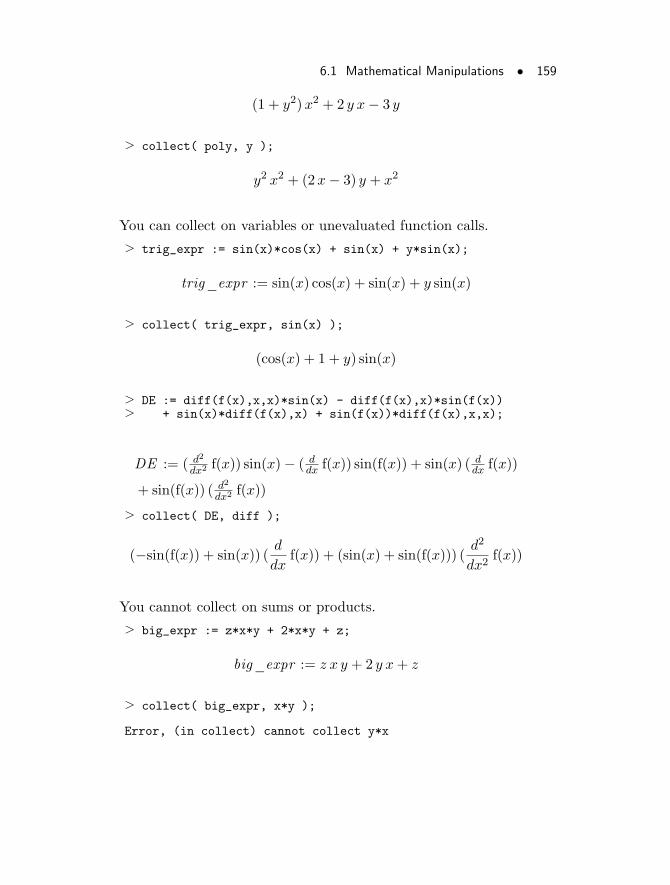
6.1 Mathematical Manipulations • 159
(1 + y2)x2 + 2 y x− 3 y
> collect( poly, y );
y2 x2 + (2x− 3) y + x2
You can collect on variables or unevaluated function calls.
> trig_expr := sin(x)*cos(x) + sin(x) + y*sin(x);
trig_expr := sin(x) cos(x) + sin(x) + y sin(x)
> collect( trig_expr, sin(x) );
(cos(x) + 1 + y) sin(x)
> DE := diff(f(x),x,x)*sin(x) - diff(f(x),x)*sin(f(x))> + sin(x)*diff(f(x),x) + sin(f(x))*diff(f(x),x,x);
DE := ( d2
dx2 f(x)) sin(x)− ( ddx f(x)) sin(f(x)) + sin(x) ( d
dx f(x))
+ sin(f(x)) ( d2
dx2 f(x))
> collect( DE, diff );
(−sin(f(x)) + sin(x)) (d
dxf(x)) + (sin(x) + sin(f(x))) (
d2
dx2f(x))
You cannot collect on sums or products.
> big_expr := z*x*y + 2*x*y + z;
big_expr := z x y + 2 y x+ z
> collect( big_expr, x*y );
Error, (in collect) cannot collect y*x
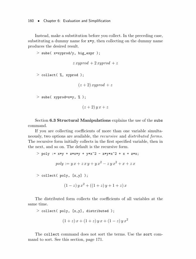
160 • Chapter 6: Evaluation and Simplification
Instead, make a substitution before you collect. In the preceding case,substituting a dummy name for x*y, then collecting on the dummy nameproduces the desired result.
> subs( x=xyprod/y, big_expr );
z xyprod + 2 xyprod + z
> collect( %, xyprod );
(z + 2) xyprod + z
> subs( xyprod=x*y, % );
(z + 2) y x+ z
Section 6.3 Structural Manipulations explains the use of the subscommand.
If you are collecting coefficients of more than one variable simulta-neously, two options are available, the recursive and distributed forms.The recursive form initially collects in the first specified variable, then inthe next, and so on. The default is the recursive form.
> poly := x*y + z*x*y + y*x^2 - z*y*x^2 + x + z*x;
poly := y x+ z x y + y x2 − z y x2 + x+ z x
> collect( poly, [x,y] );
(1− z) y x2 + ((1 + z) y + 1 + z)x
The distributed form collects the coefficients of all variables at thesame time.
> collect( poly, [x,y], distributed );
(1 + z)x+ (1 + z) y x+ (1− z) y x2
The collect command does not sort the terms. Use the sort com-mand to sort. See this section, page 171.
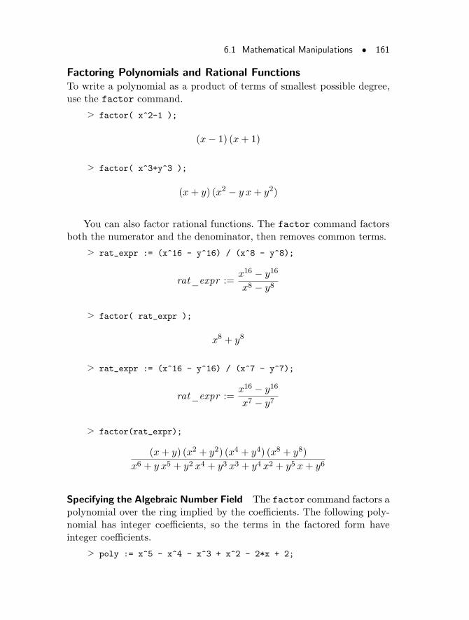
6.1 Mathematical Manipulations • 161
Factoring Polynomials and Rational FunctionsTo write a polynomial as a product of terms of smallest possible degree,use the factor command.
> factor( x^2-1 );
(x− 1) (x+ 1)
> factor( x^3+y^3 );
(x+ y) (x2 − y x+ y2)
You can also factor rational functions. The factor command factorsboth the numerator and the denominator, then removes common terms.
> rat_expr := (x^16 - y^16) / (x^8 - y^8);
rat_expr :=x16 − y16
x8 − y8
> factor( rat_expr );
x8 + y8
> rat_expr := (x^16 - y^16) / (x^7 - y^7);
rat_expr :=x16 − y16
x7 − y7
> factor(rat_expr);
(x+ y) (x2 + y2) (x4 + y4) (x8 + y8)
x6 + y x5 + y2 x4 + y3 x3 + y4 x2 + y5 x+ y6
Specifying the Algebraic Number Field The factor command factors apolynomial over the ring implied by the coefficients. The following poly-nomial has integer coefficients, so the terms in the factored form haveinteger coefficients.
> poly := x^5 - x^4 - x^3 + x^2 - 2*x + 2;
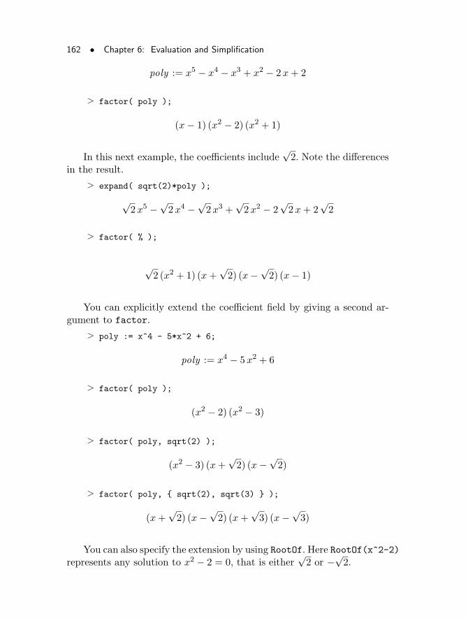
162 • Chapter 6: Evaluation and Simplification
poly := x5 − x4 − x3 + x2 − 2x+ 2
> factor( poly );
(x− 1) (x2 − 2) (x2 + 1)
In this next example, the coefficients include√2. Note the differences
in the result.
> expand( sqrt(2)*poly );
√2x5 −
√2x4 −
√2x3 +
√2x2 − 2
√2x+ 2
√2
> factor( % );
√2 (x2 + 1) (x+
√2) (x−
√2) (x− 1)
You can explicitly extend the coefficient field by giving a second ar-gument to factor.
> poly := x^4 - 5*x^2 + 6;
poly := x4 − 5x2 + 6
> factor( poly );
(x2 − 2) (x2 − 3)
> factor( poly, sqrt(2) );
(x2 − 3) (x+√2) (x−
√2)
> factor( poly, { sqrt(2), sqrt(3) } );
(x+√2) (x−
√2) (x+
√3) (x−
√3)
You can also specify the extension by using RootOf. Here RootOf(x^2-2)represents any solution to x2 − 2 = 0, that is either
√2 or −
√2.
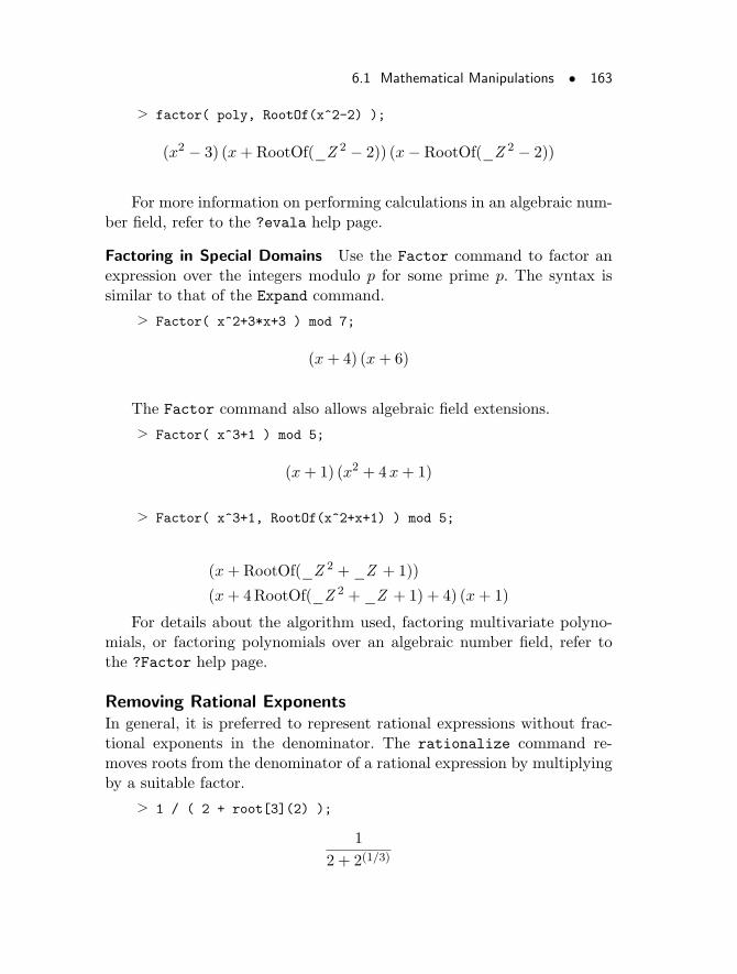
6.1 Mathematical Manipulations • 163
> factor( poly, RootOf(x^2-2) );
(x2 − 3) (x+RootOf(_Z 2 − 2)) (x− RootOf(_Z 2 − 2))
For more information on performing calculations in an algebraic num-ber field, refer to the ?evala help page.
Factoring in Special Domains Use the Factor command to factor anexpression over the integers modulo p for some prime p. The syntax issimilar to that of the Expand command.
> Factor( x^2+3*x+3 ) mod 7;
(x+ 4) (x+ 6)
The Factor command also allows algebraic field extensions.
> Factor( x^3+1 ) mod 5;
(x+ 1) (x2 + 4x+ 1)
> Factor( x^3+1, RootOf(x^2+x+1) ) mod 5;
(x+RootOf(_Z 2 +_Z + 1))
(x+ 4RootOf(_Z 2 +_Z + 1) + 4) (x+ 1)
For details about the algorithm used, factoring multivariate polyno-mials, or factoring polynomials over an algebraic number field, refer tothe ?Factor help page.
Removing Rational ExponentsIn general, it is preferred to represent rational expressions without frac-tional exponents in the denominator. The rationalize command re-moves roots from the denominator of a rational expression by multiplyingby a suitable factor.
> 1 / ( 2 + root[3](2) );
1
2 + 2(1/3)
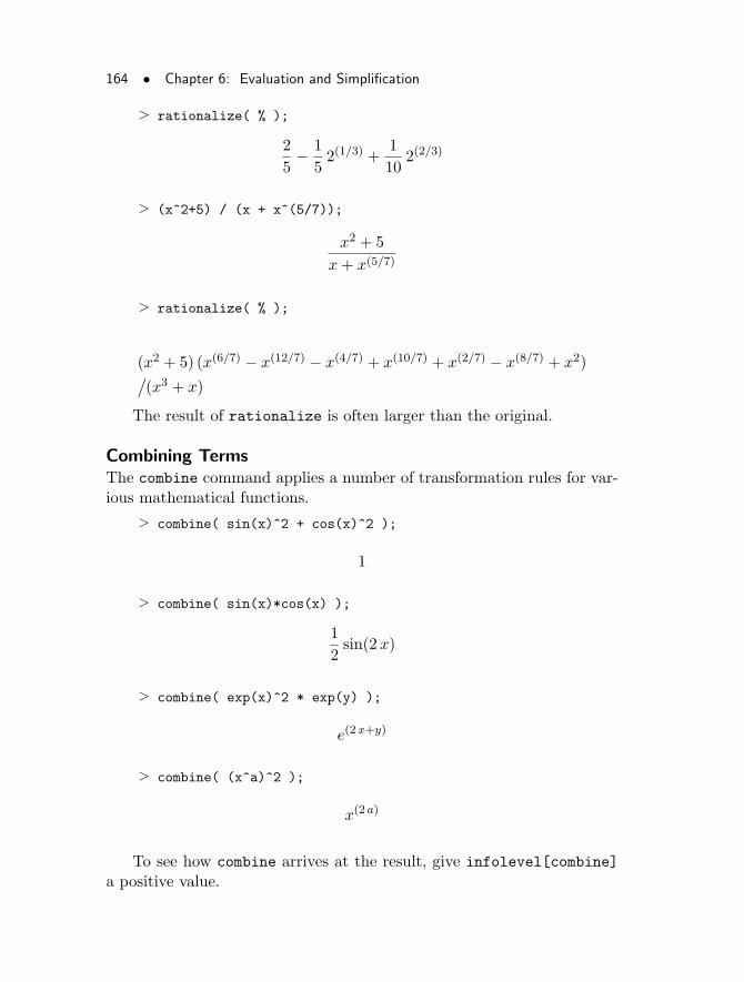
164 • Chapter 6: Evaluation and Simplification
> rationalize( % );
2
5− 1
52(1/3) +
1
102(2/3)
> (x^2+5) / (x + x^(5/7));
x2 + 5
x+ x(5/7)
> rationalize( % );
(x2 + 5) (x(6/7) − x(12/7) − x(4/7) + x(10/7) + x(2/7) − x(8/7) + x2)/
(x3 + x)
The result of rationalize is often larger than the original.
Combining TermsThe combine command applies a number of transformation rules for var-ious mathematical functions.
> combine( sin(x)^2 + cos(x)^2 );
1
> combine( sin(x)*cos(x) );
1
2sin(2x)
> combine( exp(x)^2 * exp(y) );
e(2x+y)
> combine( (x^a)^2 );
x(2 a)
To see how combine arrives at the result, give infolevel[combine]
a positive value.
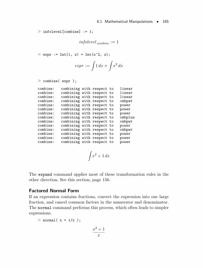
6.1 Mathematical Manipulations • 165
> infolevel[combine] := 1;
infolevel combine := 1
> expr := Int(1, x) + Int(x^2, x);
expr :=
∫
1 dx+
∫
x2 dx
> combine( expr );
combine: combining with respect to linearcombine: combining with respect to linearcombine: combining with respect to linearcombine: combining with respect to cmbpwrcombine: combining with respect to powercombine: combining with respect to powercombine: combining with respect to powercombine: combining with respect to cmbpluscombine: combining with respect to cmbpwrcombine: combining with respect to powercombine: combining with respect to cmbpwrcombine: combining with respect to powercombine: combining with respect to powercombine: combining with respect to power
∫
x2 + 1 dx
The expand command applies most of these transformation rules in theother direction. See this section, page 156.
Factored Normal FormIf an expression contains fractions, convert the expression into one largefraction, and cancel common factors in the numerator and denominator.The normal command performs this process, which often leads to simplerexpressions.
> normal( x + 1/x );
x2 + 1
x
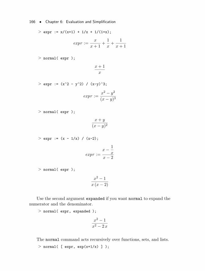
166 • Chapter 6: Evaluation and Simplification
> expr := x/(x+1) + 1/x + 1/(1+x);
expr :=x
x+ 1+
1
x+
1
x+ 1
> normal( expr );
x+ 1
x
> expr := (x^2 - y^2) / (x-y)^3;
expr :=x2 − y2
(x− y)3
> normal( expr );
x+ y
(x− y)2
> expr := (x - 1/x) / (x-2);
expr :=x− 1
xx− 2
> normal( expr );
x2 − 1
x (x− 2)
Use the second argument expanded if you want normal to expand thenumerator and the denominator.
> normal( expr, expanded );
x2 − 1
x2 − 2x
The normal command acts recursively over functions, sets, and lists.
> normal( [ expr, exp(x+1/x) ] );
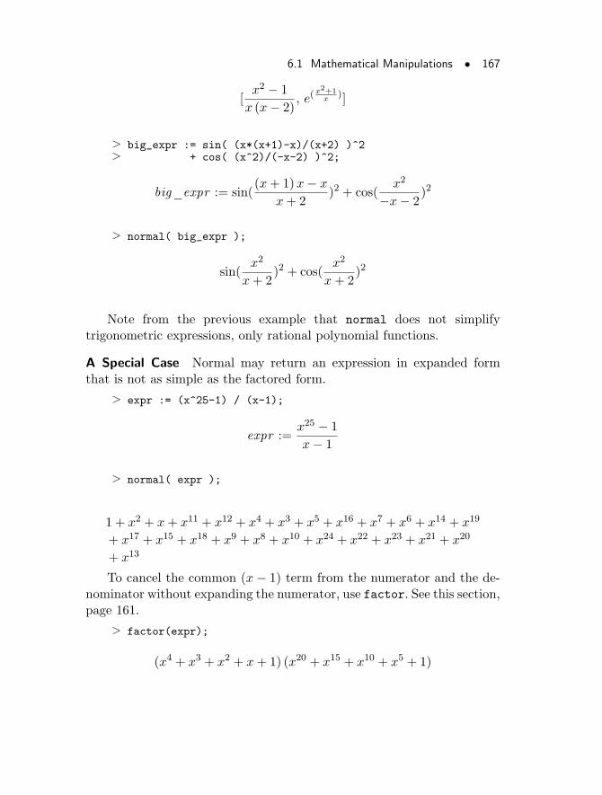
6.1 Mathematical Manipulations • 167
[x2 − 1
x (x− 2), e(
x2+1x
)]
> big_expr := sin( (x*(x+1)-x)/(x+2) )^2> + cos( (x^2)/(-x-2) )^2;
big_expr := sin((x+ 1)x− x
x+ 2)2 + cos(
x2
−x− 2)2
> normal( big_expr );
sin(x2
x+ 2)2 + cos(
x2
x+ 2)2
Note from the previous example that normal does not simplifytrigonometric expressions, only rational polynomial functions.
A Special Case Normal may return an expression in expanded formthat is not as simple as the factored form.
> expr := (x^25-1) / (x-1);
expr :=x25 − 1
x− 1
> normal( expr );
1 + x2 + x+ x11 + x12 + x4 + x3 + x5 + x16 + x7 + x6 + x14 + x19
+ x17 + x15 + x18 + x9 + x8 + x10 + x24 + x22 + x23 + x21 + x20
+ x13
To cancel the common (x− 1) term from the numerator and the de-nominator without expanding the numerator, use factor. See this section,page 161.
> factor(expr);
(x4 + x3 + x2 + x+ 1) (x20 + x15 + x10 + x5 + 1)
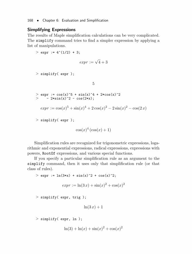
168 • Chapter 6: Evaluation and Simplification
Simplifying ExpressionsThe results of Maple simplification calculations can be very complicated.The simplify command tries to find a simpler expression by applying alist of manipulations.
> expr := 4^(1/2) + 3;
expr :=√4 + 3
> simplify( expr );
5
> expr := cos(x)^5 + sin(x)^4 + 2*cos(x)^2> - 2*sin(x)^2 - cos(2*x);
expr := cos(x)5 + sin(x)4 + 2 cos(x)2 − 2 sin(x)2 − cos(2x)
> simplify( expr );
cos(x)4 (cos(x) + 1)
Simplification rules are recognized for trigonometric expressions, loga-rithmic and exponential expressions, radical expressions, expressions withpowers, RootOf expressions, and various special functions.
If you specify a particular simplification rule as an argument to thesimplify command, then it uses only that simplification rule (or thatclass of rules).
> expr := ln(3*x) + sin(x)^2 + cos(x)^2;
expr := ln(3x) + sin(x)2 + cos(x)2
> simplify( expr, trig );
ln(3x) + 1
> simplify( expr, ln );
ln(3) + ln(x) + sin(x)2 + cos(x)2
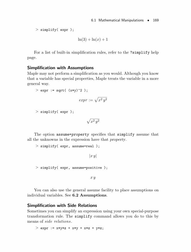
6.1 Mathematical Manipulations • 169
> simplify( expr );
ln(3) + ln(x) + 1
For a list of built-in simplification rules, refer to the ?simplify helppage.
Simplification with AssumptionsMaple may not perform a simplification as you would. Although you knowthat a variable has special properties, Maple treats the variable in a moregeneral way.
> expr := sqrt( (x*y)^2 );
expr :=√
x2 y2
> simplify( expr );
√
x2 y2
The option assume=property specifies that simplify assume thatall the unknowns in the expression have that property.
> simplify( expr, assume=real );
|x y|
> simplify( expr, assume=positive );
x y
You can also use the general assume facility to place assumptions onindividual variables. See 6.2 Assumptions.
Simplification with Side RelationsSometimes you can simplify an expression using your own special-purposetransformation rule. The simplify command allows you do to this bymeans of side relations .
> expr := x*y*z + x*y + x*z + y*z;
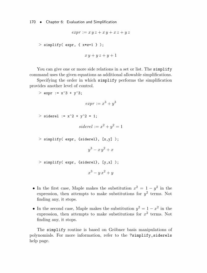
170 • Chapter 6: Evaluation and Simplification
expr := x y z + x y + x z + y z
> simplify( expr, { x*z=1 } );
x y + y z + y + 1
You can give one or more side relations in a set or list. The simplifycommand uses the given equations as additional allowable simplifications.
Specifying the order in which simplify performs the simplificationprovides another level of control.
> expr := x^3 + y^3;
expr := x3 + y3
> siderel := x^2 + y^2 = 1;
siderel := x2 + y2 = 1
> simplify( expr, {siderel}, [x,y] );
y3 − x y2 + x
> simplify( expr, {siderel}, [y,x] );
x3 − y x2 + y
• In the first case, Maple makes the substitution x2 = 1 − y2 in theexpression, then attempts to make substitutions for y2 terms. Notfinding any, it stops.
• In the second case, Maple makes the substitution y2 = 1 − x2 in theexpression, then attempts to make substitutions for x2 terms. Notfinding any, it stops.
The simplify routine is based on Grobner basis manipulations ofpolynomials. For more information, refer to the ?simplify,siderels
help page.
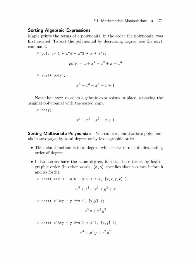
6.1 Mathematical Manipulations • 171
Sorting Algebraic ExpressionsMaple prints the terms of a polynomial in the order the polynomial wasfirst created. To sort the polynomial by decreasing degree, use the sort
command.
> poly := 1 + x^4 - x^2 + x + x^3;
poly := 1 + x4 − x2 + x+ x3
> sort( poly );
x4 + x3 − x2 + x+ 1
Note that sort reorders algebraic expressions in place, replacing theoriginal polynomial with the sorted copy.
> poly;
x4 + x3 − x2 + x+ 1
Sorting Multivariate Polynomials You can sort multivariate polynomi-als in two ways, by total degree or by lexicographic order.
• The default method is total degree, which sorts terms into descendingorder of degree.
• If two terms have the same degree, it sorts those terms by lexico-graphic order (in other words, [a,b] specifies that a comes before band so forth).
> sort( x+x^3 + w^5 + y^2 + z^4, [w,x,y,z] );
w5 + z4 + x3 + y2 + x
> sort( x^3*y + y^2*x^2, [x,y] );
x3 y + x2 y2
> sort( x^3*y + y^2*x^2 + x^4, [x,y] );
x4 + x3 y + x2 y2
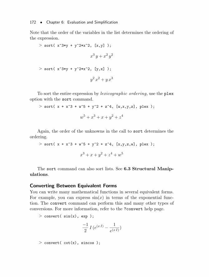
172 • Chapter 6: Evaluation and Simplification
Note that the order of the variables in the list determines the ordering ofthe expression.
> sort( x^3*y + y^2*x^2, [x,y] );
x3 y + x2 y2
> sort( x^3*y + y^2*x^2, [y,x] );
y2 x2 + y x3
To sort the entire expression by lexicographic ordering, use the plexoption with the sort command.
> sort( x + x^3 + w^5 + y^2 + z^4, [w,x,y,z], plex );
w5 + x3 + x+ y2 + z4
Again, the order of the unknowns in the call to sort determines theordering.
> sort( x + x^3 + w^5 + y^2 + z^4, [x,y,z,w], plex );
x3 + x+ y2 + z4 + w5
The sort command can also sort lists. See 6.3 Structural Manip-ulations.
Converting Between Equivalent FormsYou can write many mathematical functions in several equivalent forms.For example, you can express sin(x) in terms of the exponential func-tion. The convert command can perform this and many other types ofconversions. For more information, refer to the ?convert help page.
> convert( sin(x), exp );
−1
2I (e(x I) − 1
e(x I))
> convert( cot(x), sincos );
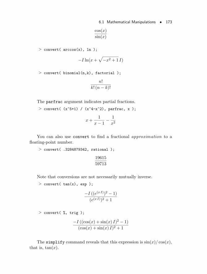
6.1 Mathematical Manipulations • 173
cos(x)
sin(x)
> convert( arccos(x), ln );
−I ln(x+√
−x2 + 1 I)
> convert( binomial(n,k), factorial );
n!
k! (n− k)!
The parfrac argument indicates partial fractions.
> convert( (x^5+1) / (x^4-x^2), parfrac, x );
x+1
x− 1− 1
x2
You can also use convert to find a fractional approximation to afloating-point number.
> convert( .3284879342, rational );
19615
59713
Note that conversions are not necessarily mutually inverse.
> convert( tan(x), exp );
−I ((e(x I))2 − 1)
(e(x I))2 + 1
> convert( %, trig );
−I ((cos(x) + sin(x) I)2 − 1)
(cos(x) + sin(x) I)2 + 1
The simplify command reveals that this expression is sin(x)/ cos(x),that is, tan(x).
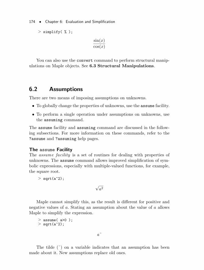
174 • Chapter 6: Evaluation and Simplification
> simplify( % );
sin(x)
cos(x)
You can also use the convert command to perform structural manip-ulations on Maple objects. See 6.3 Structural Manipulations.
6.2 Assumptions
There are two means of imposing assumptions on unknowns.
• To globally change the properties of unknowns, use the assume facility.
• To perform a single operation under assumptions on unknowns, usethe assuming command.
The assume facility and assuming command are discussed in the follow-ing subsections. For more information on these commands, refer to the?assume and ?assuming help pages.
The assume FacilityThe assume facility is a set of routines for dealing with properties ofunknowns. The assume command allows improved simplification of sym-bolic expressions, especially with multiple-valued functions, for example,the square root.
> sqrt(a^2);
√a2
Maple cannot simplify this, as the result is different for positive andnegative values of a. Stating an assumption about the value of a allowsMaple to simplify the expression.
> assume( a>0 );> sqrt(a^2);
a~
The tilde (~) on a variable indicates that an assumption has beenmade about it. New assumptions replace old ones.
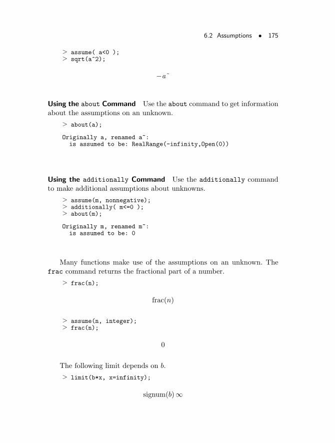
6.2 Assumptions • 175
> assume( a<0 );> sqrt(a^2);
−a~
Using the about Command Use the about command to get informationabout the assumptions on an unknown.
> about(a);
Originally a, renamed a~:is assumed to be: RealRange(-infinity,Open(0))
Using the additionally Command Use the additionally commandto make additional assumptions about unknowns.
> assume(m, nonnegative);> additionally( m<=0 );> about(m);
Originally m, renamed m~:is assumed to be: 0
Many functions make use of the assumptions on an unknown. Thefrac command returns the fractional part of a number.
> frac(n);
frac(n)
> assume(n, integer);> frac(n);
0
The following limit depends on b.
> limit(b*x, x=infinity);
signum(b)∞
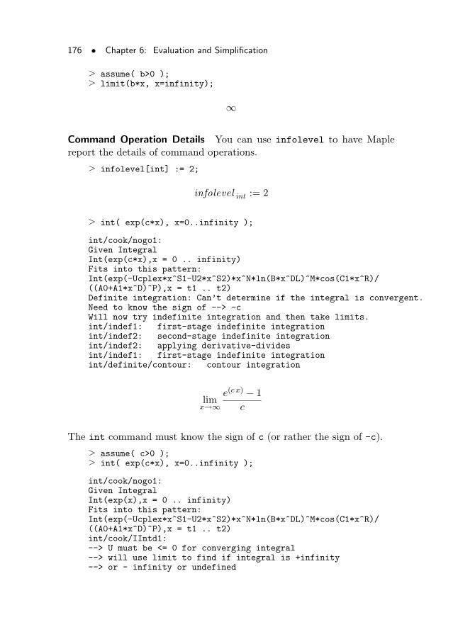
176 • Chapter 6: Evaluation and Simplification
> assume( b>0 );> limit(b*x, x=infinity);
∞
Command Operation Details You can use infolevel to have Maplereport the details of command operations.
> infolevel[int] := 2;
infolevel int := 2
> int( exp(c*x), x=0..infinity );
int/cook/nogo1:Given IntegralInt(exp(c*x),x = 0 .. infinity)Fits into this pattern:Int(exp(-Ucplex*x^S1-U2*x^S2)*x^N*ln(B*x^DL)^M*cos(C1*x^R)/((A0+A1*x^D)^P),x = t1 .. t2)Definite integration: Can’t determine if the integral is convergent.Need to know the sign of --> -cWill now try indefinite integration and then take limits.int/indef1: first-stage indefinite integrationint/indef2: second-stage indefinite integrationint/indef2: applying derivative-dividesint/indef1: first-stage indefinite integrationint/definite/contour: contour integration
limx→∞
e(c x) − 1
c
The int command must know the sign of c (or rather the sign of -c).
> assume( c>0 );> int( exp(c*x), x=0..infinity );
int/cook/nogo1:Given IntegralInt(exp(x),x = 0 .. infinity)Fits into this pattern:Int(exp(-Ucplex*x^S1-U2*x^S2)*x^N*ln(B*x^DL)^M*cos(C1*x^R)/((A0+A1*x^D)^P),x = t1 .. t2)int/cook/IIntd1:--> U must be <= 0 for converging integral--> will use limit to find if integral is +infinity--> or - infinity or undefined
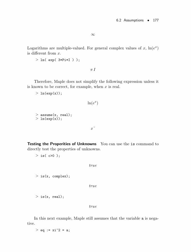
6.2 Assumptions • 177
∞
Logarithms are multiple-valued. For general complex values of x, ln(ex)is different from x.
> ln( exp( 3*Pi*I ) );
π I
Therefore, Maple does not simplify the following expression unless itis known to be correct, for example, when x is real.
> ln(exp(x));
ln(ex)
> assume(x, real);> ln(exp(x));
x~
Testing the Properities of Unknowns You can use the is command todirectly test the properties of unknowns.
> is( c>0 );
true
> is(x, complex);
true
> is(x, real);
true
In this next example, Maple still assumes that the variable a is nega-tive.
> eq := xi^2 = a;
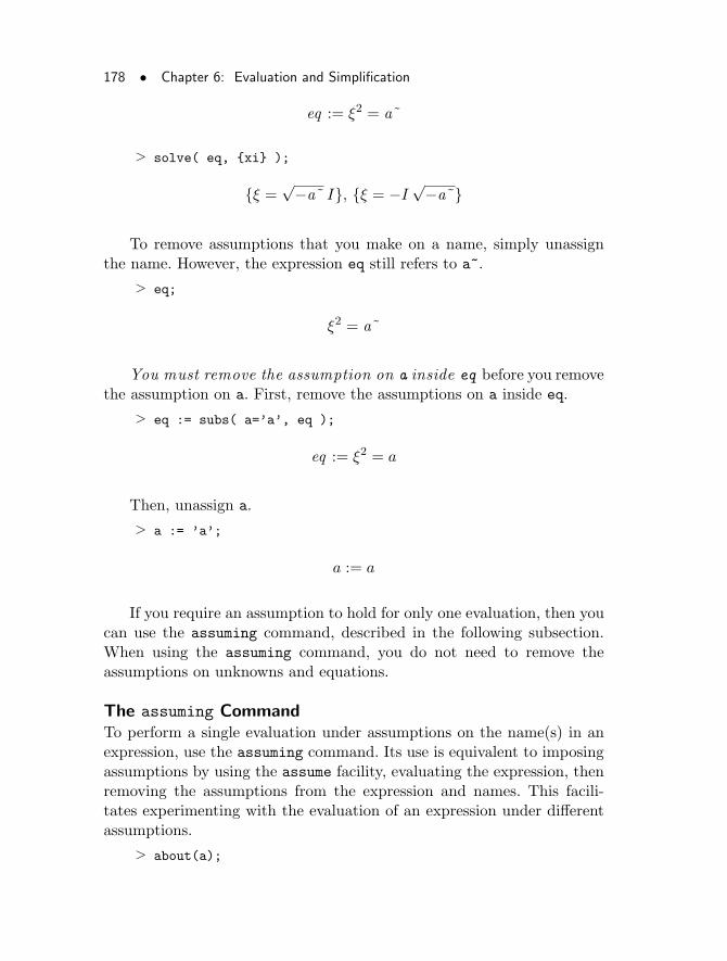
178 • Chapter 6: Evaluation and Simplification
eq := ξ2 = a~
> solve( eq, {xi} );
{ξ =√−a~ I}, {ξ = −I
√−a~}
To remove assumptions that you make on a name, simply unassignthe name. However, the expression eq still refers to a~.
> eq;
ξ2 = a~
You must remove the assumption on a inside eq before you removethe assumption on a. First, remove the assumptions on a inside eq.
> eq := subs( a=’a’, eq );
eq := ξ2 = a
Then, unassign a.
> a := ’a’;
a := a
If you require an assumption to hold for only one evaluation, then youcan use the assuming command, described in the following subsection.When using the assuming command, you do not need to remove theassumptions on unknowns and equations.
The assuming CommandTo perform a single evaluation under assumptions on the name(s) in anexpression, use the assuming command. Its use is equivalent to imposingassumptions by using the assume facility, evaluating the expression, thenremoving the assumptions from the expression and names. This facili-tates experimenting with the evaluation of an expression under differentassumptions.
> about(a);
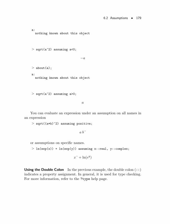
6.2 Assumptions • 179
a:nothing known about this object
> sqrt(a^2) assuming a<0;
−a
> about(a);
a:nothing known about this object
> sqrt(a^2) assuming a>0;
a
You can evaluate an expression under an assumption on all names inan expression
> sqrt((a*b)^2) assuming positive;
a b~
or assumptions on specific names.
> ln(exp(x)) + ln(exp(y)) assuming x::real, y::complex;
x~ + ln(ey)
Using the Double Colon In the previous example, the double colon (::)indicates a property assignment. In general, it is used for type checking.For more information, refer to the ?type help page.
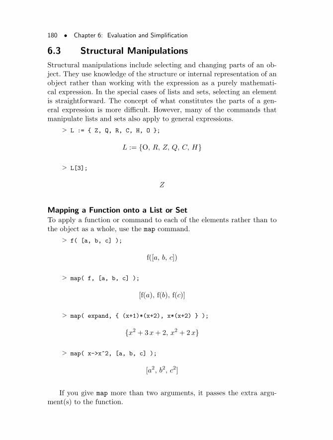
180 • Chapter 6: Evaluation and Simplification
6.3 Structural Manipulations
Structural manipulations include selecting and changing parts of an ob-ject. They use knowledge of the structure or internal representation of anobject rather than working with the expression as a purely mathemati-cal expression. In the special cases of lists and sets, selecting an elementis straightforward. The concept of what constitutes the parts of a gen-eral expression is more difficult. However, many of the commands thatmanipulate lists and sets also apply to general expressions.
> L := { Z, Q, R, C, H, O };
L := {O, R, Z, Q, C, H}
> L[3];
Z
Mapping a Function onto a List or SetTo apply a function or command to each of the elements rather than tothe object as a whole, use the map command.
> f( [a, b, c] );
f([a, b, c])
> map( f, [a, b, c] );
[f(a), f(b), f(c)]
> map( expand, { (x+1)*(x+2), x*(x+2) } );
{x2 + 3x+ 2, x2 + 2x}
> map( x->x^2, [a, b, c] );
[a2, b2, c2]
If you give map more than two arguments, it passes the extra argu-ment(s) to the function.
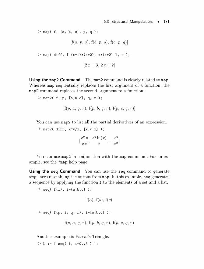
6.3 Structural Manipulations • 181
> map( f, [a, b, c], p, q );
[f(a, p, q), f(b, p, q), f(c, p, q)]
> map( diff, [ (x+1)*(x+2), x*(x+2) ], x );
[2x+ 3, 2x+ 2]
Using the map2 Command The map2 command is closely related to map.Whereas map sequentially replaces the first argument of a function, themap2 command replaces the second argument to a function.
> map2( f, p, [a,b,c], q, r );
[f(p, a, q, r), f(p, b, q, r), f(p, c, q, r)]
You can use map2 to list all the partial derivatives of an expression.
> map2( diff, x^y/z, [x,y,z] );
[xy y
x z,xy ln(x)
z, −xy
z2]
You can use map2 in conjunction with the map command. For an ex-ample, see the ?map help page.
Using the seq Command You can use the seq command to generatesequences resembling the output from map. In this example, seq generatesa sequence by applying the function f to the elements of a set and a list.
> seq( f(i), i={a,b,c} );
f(a), f(b), f(c)
> seq( f(p, i, q, r), i=[a,b,c] );
f(p, a, q, r), f(p, b, q, r), f(p, c, q, r)
Another example is Pascal’s Triangle.
> L := [ seq( i, i=0..5 ) ];
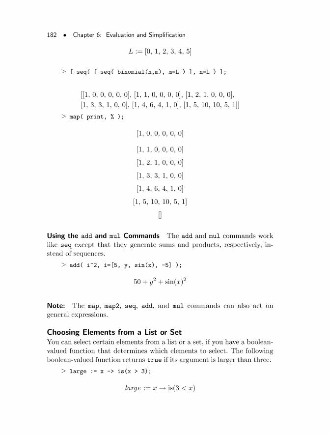
182 • Chapter 6: Evaluation and Simplification
L := [0, 1, 2, 3, 4, 5]
> [ seq( [ seq( binomial(n,m), m=L ) ], n=L ) ];
[[1, 0, 0, 0, 0, 0], [1, 1, 0, 0, 0, 0], [1, 2, 1, 0, 0, 0],
[1, 3, 3, 1, 0, 0], [1, 4, 6, 4, 1, 0], [1, 5, 10, 10, 5, 1]]
> map( print, % );
[1, 0, 0, 0, 0, 0]
[1, 1, 0, 0, 0, 0]
[1, 2, 1, 0, 0, 0]
[1, 3, 3, 1, 0, 0]
[1, 4, 6, 4, 1, 0]
[1, 5, 10, 10, 5, 1]
[]
Using the add and mul Commands The add and mul commands worklike seq except that they generate sums and products, respectively, in-stead of sequences.
> add( i^2, i=[5, y, sin(x), -5] );
50 + y2 + sin(x)2
Note: The map, map2, seq, add, and mul commands can also act ongeneral expressions.
Choosing Elements from a List or SetYou can select certain elements from a list or a set, if you have a boolean-valued function that determines which elements to select. The followingboolean-valued function returns true if its argument is larger than three.
> large := x -> is(x > 3);
large := x → is(3 < x)
6.3 Structural Manipulations • 183
Use the select command to choose the elements in a list or set thatsatisfy large.
> L := [ 8, 2.95, Pi, sin(9) ];
L := [8, 2.95, π, sin(9)]
> select( large, L );
[8, π]
Using the remove Command The remove command removes the ele-ments from L that satisfy large and displays as output the remainingelements.
> remove( large, L );
[2.95, sin(9)]
Using the selectremove Command To perform operations of both theselect and remove commands simultaneously, use the selectremove
command.
> selectremove( large, L);
[8, π], [2.95, sin(9)]
Using the type Command Use the type command to determine thetype of an expression.
> type( 3, numeric );
true
> type( cos(1), numeric );
false
The syntax of select here passes the third argument, numeric, tothe type command.
184 • Chapter 6: Evaluation and Simplification
> select( type, L, numeric );
[8, 2.95]
For more information on types and using select and remove on ageneral expression, see this section, pages 190–196.
Merging Two ListsSometimes you need to merge two lists. Here is a list of x-values and alist of y-values.
> X := [ seq( ithprime(i), i=1..6 ) ];
X := [2, 3, 5, 7, 11, 13]
> Y := [ seq( binomial(6, i), i=1..6 ) ];
Y := [6, 15, 20, 15, 6, 1]
To plot the y-values against the x-values, construct a list of lists: [[x1,y1], [x2,y2], ... ]. That is, for each pair of values, construct atwo-element list.
> pair := (x,y) -> [x, y];
pair := (x, y) → [x, y]
Using the zip Command The zip command can merge the lists X andY according to the binary function pair.
> P := zip( pair, X, Y );
P := [[2, 6], [3, 15], [5, 20], [7, 15], [11, 6], [13, 1]]
> plot( P );
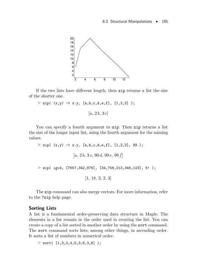
6.3 Structural Manipulations • 185
2468
101214161820
2 4 6 8 10 12
If the two lists have different length, then zip returns a list the sizeof the shorter one.
> zip( (x,y) -> x.y, [a,b,c,d,e,f], [1,2,3] );
[a, 2 b, 3 c]
You can specify a fourth argument to zip. Then zip returns a listthe size of the longer input list, using the fourth argument for the missingvalues.
> zip( (x,y) -> x.y, [a,b,c,d,e,f], [1,2,3], 99 );
[a, 2 b, 3 c, 99 d, 99 e, 99 f ]
> zip( igcd, [7657,342,876], [34,756,213,346,123], 6! );
[1, 18, 3, 2, 3]
The zip command can also merge vectors. For more information, referto the ?zip help page.
Sorting ListsA list is a fundamental order-preserving data structure in Maple. Theelements in a list remain in the order used in creating the list. You cancreate a copy of a list sorted in another order by using the sort command.The sort command sorts lists, among other things, in ascending order.It sorts a list of numbers in numerical order.
> sort( [1,3,2,4,5,3,6,3,6] );
186 • Chapter 6: Evaluation and Simplification
[1, 2, 3, 3, 3, 4, 5, 6, 6]
The sort command also sorts a list of strings in lexicographic order.
> sort( ["Mary", "had", "a", "little", "lamb"] );
[“Mary”, “a”, “had”, “lamb”, “little”]
Session Dependent Machine Addresses If a list contains both numbersand strings, or expressions different from numbers and strings, sort usesthe machine addresses, which are session dependent.
> sort( [x, 1, "apple"] );
[1, x, “apple”]
> sort( [-5, 10, sin(34)] );
[10, sin(34), −5]
Note that to Maple, π is not numeric.
> sort( [4.3, Pi, 2/3] );
[π,2
3, 4.3]
You can specify a boolean function to define an ordering for a list.The boolean function must take two arguments and return true if thefirst argument precedes the second. You can use this to sort a list ofnumbers in descending order.
> sort( [3.12, 1, 1/2], (x,y) -> evalb( x>y ) );
[3.12, 1,1
2]
Using the is Command The is command can compare constants likeπ and sin(5) with pure numbers.
> bf := (x,y) -> is( x < y );
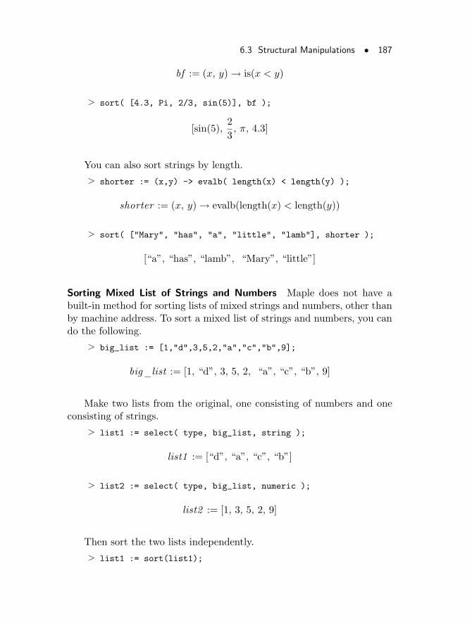
6.3 Structural Manipulations • 187
bf := (x, y) → is(x < y)
> sort( [4.3, Pi, 2/3, sin(5)], bf );
[sin(5),2
3, π, 4.3]
You can also sort strings by length.
> shorter := (x,y) -> evalb( length(x) < length(y) );
shorter := (x, y) → evalb(length(x) < length(y))
> sort( ["Mary", "has", "a", "little", "lamb"], shorter );
[“a”, “has”, “lamb”, “Mary”, “little”]
Sorting Mixed List of Strings and Numbers Maple does not have abuilt-in method for sorting lists of mixed strings and numbers, other thanby machine address. To sort a mixed list of strings and numbers, you cando the following.
> big_list := [1,"d",3,5,2,"a","c","b",9];
big_list := [1, “d”, 3, 5, 2, “a”, “c”, “b”, 9]
Make two lists from the original, one consisting of numbers and oneconsisting of strings.
> list1 := select( type, big_list, string );
list1 := [“d”, “a”, “c”, “b”]
> list2 := select( type, big_list, numeric );
list2 := [1, 3, 5, 2, 9]
Then sort the two lists independently.
> list1 := sort(list1);
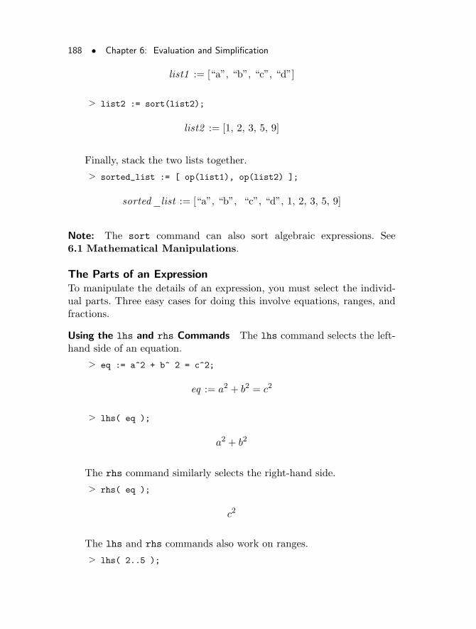
188 • Chapter 6: Evaluation and Simplification
list1 := [“a”, “b”, “c”, “d”]
> list2 := sort(list2);
list2 := [1, 2, 3, 5, 9]
Finally, stack the two lists together.
> sorted_list := [ op(list1), op(list2) ];
sorted_list := [“a”, “b”, “c”, “d”, 1, 2, 3, 5, 9]
Note: The sort command can also sort algebraic expressions. See6.1 Mathematical Manipulations.
The Parts of an ExpressionTo manipulate the details of an expression, you must select the individ-ual parts. Three easy cases for doing this involve equations, ranges, andfractions.
Using the lhs and rhs Commands The lhs command selects the left-hand side of an equation.
> eq := a^2 + b^ 2 = c^2;
eq := a2 + b2 = c2
> lhs( eq );
a2 + b2
The rhs command similarly selects the right-hand side.
> rhs( eq );
c2
The lhs and rhs commands also work on ranges.
> lhs( 2..5 );
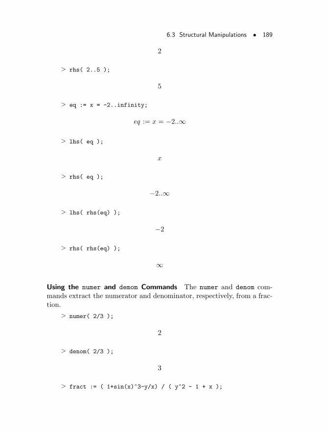
6.3 Structural Manipulations • 189
2
> rhs( 2..5 );
5
> eq := x = -2..infinity;
eq := x = −2..∞
> lhs( eq );
x
> rhs( eq );
−2..∞
> lhs( rhs(eq) );
−2
> rhs( rhs(eq) );
∞
Using the numer and demom Commands The numer and denom com-mands extract the numerator and denominator, respectively, from a frac-tion.
> numer( 2/3 );
2
> denom( 2/3 );
3
> fract := ( 1+sin(x)^3-y/x) / ( y^2 - 1 + x );
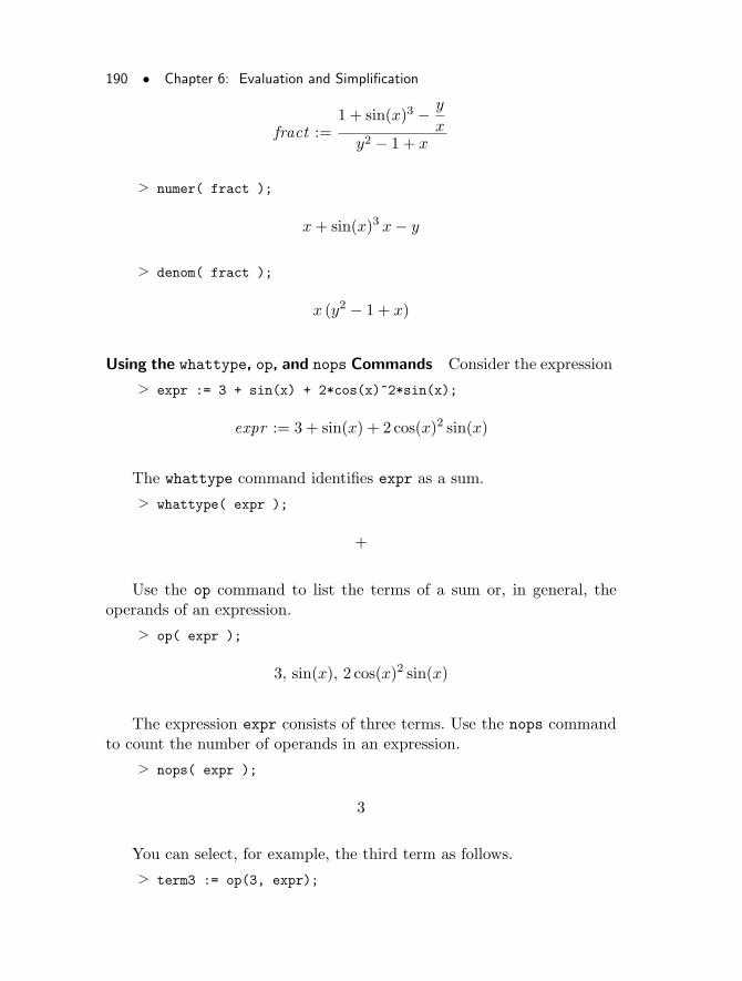
190 • Chapter 6: Evaluation and Simplification
fract :=1 + sin(x)3 − y
xy2 − 1 + x
> numer( fract );
x+ sin(x)3 x− y
> denom( fract );
x (y2 − 1 + x)
Using the whattype, op, and nops Commands Consider the expression
> expr := 3 + sin(x) + 2*cos(x)^2*sin(x);
expr := 3 + sin(x) + 2 cos(x)2 sin(x)
The whattype command identifies expr as a sum.
> whattype( expr );
+
Use the op command to list the terms of a sum or, in general, theoperands of an expression.
> op( expr );
3, sin(x), 2 cos(x)2 sin(x)
The expression expr consists of three terms. Use the nops commandto count the number of operands in an expression.
> nops( expr );
3
You can select, for example, the third term as follows.
> term3 := op(3, expr);
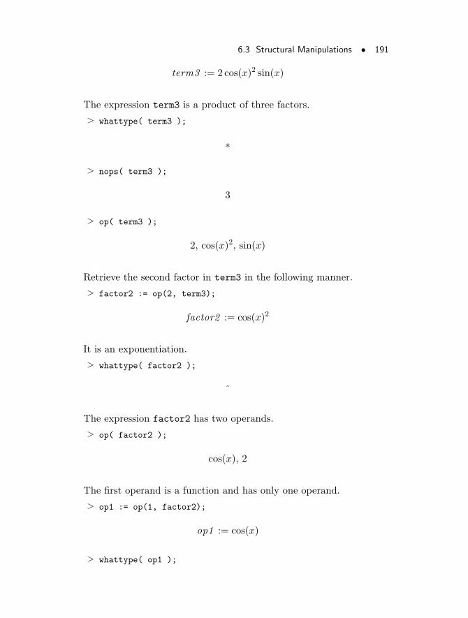
6.3 Structural Manipulations • 191
term3 := 2 cos(x)2 sin(x)
The expression term3 is a product of three factors.
> whattype( term3 );
∗
> nops( term3 );
3
> op( term3 );
2, cos(x)2, sin(x)
Retrieve the second factor in term3 in the following manner.
> factor2 := op(2, term3);
factor2 := cos(x)2
It is an exponentiation.
> whattype( factor2 );
^
The expression factor2 has two operands.
> op( factor2 );
cos(x), 2
The first operand is a function and has only one operand.
> op1 := op(1, factor2);
op1 := cos(x)
> whattype( op1 );
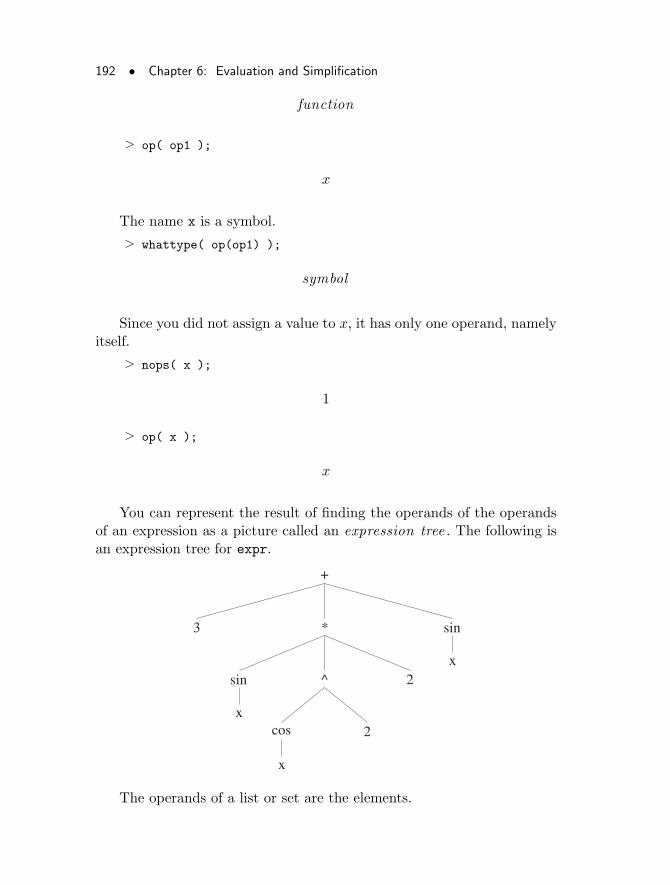
192 • Chapter 6: Evaluation and Simplification
function
> op( op1 );
x
The name x is a symbol.
> whattype( op(op1) );
symbol
Since you did not assign a value to x, it has only one operand, namelyitself.
> nops( x );
1
> op( x );
x
You can represent the result of finding the operands of the operandsof an expression as a picture called an expression tree . The following isan expression tree for expr.
x
x2cos
x2^sin
sin*3
+
The operands of a list or set are the elements.
6.3 Structural Manipulations • 193
> op( [a,b,c] );
a, b, c
> op( {d,e,f} );
e, d, f
This section (page 180) describes how the map command applies afunction to all the elements of a list or set. The functionality of map
extends to general expressions.
> map( f, x^2 );
f(x)f(2)
The select and remove commands, described in this section (pages 182–184) also work on general expressions.
> large := z -> evalb( is(z>3) = true );
large := z → evalb(is(3 < z) = true)
> remove( large, 5+8*sin(x) - exp(9) );
8 sin(x)− e9
Maple has many commands that can be used as the boolean functionin a call to select or remove. The has command determines whether anexpression contains a certain subexpression.
> has( x*exp(cos(t^2)), t^2 );
true
> has( x*exp(cos(t^2)), cos );
true
Some of the solutions to the following set of equations containRootOfs.
194 • Chapter 6: Evaluation and Simplification
> sol := { solve( { x^2*y^2 = b*y, x^2-y^2 = a*x },> {x,y} ) };
sol := {{y = 0, x = 0}, {y = 0, x = a}, {x = RootOf(_Z 6 − b2 − a_Z 5),
y =b
RootOf(_Z 6 − b2 − a_Z 5)2}}
To select solutions, use select and has.
> select( has, sol, RootOf );
{{x = RootOf(_Z 6 − b2 − a_Z 5),
y =b
RootOf(_Z 6 − b2 − a_Z 5)2}}
You can also select or remove subexpressions by type. The type com-mand determines if an expression is of a certain type.
> type( 3+x, ‘+‘ );
true
In this example, the select command passes its third argument, ‘+‘,to type.
> expr := ( 3+x ) * x^2 * sin( 1+sqrt(Pi) );
expr := (3 + x)x2 sin(1 +√π)
> select( type, expr, ‘+‘ );
3 + x
The hastype command determines if an expression contains a subex-pression of a certain type.
> hastype( sin( 1+sqrt(Pi) ), ‘+‘ );
true
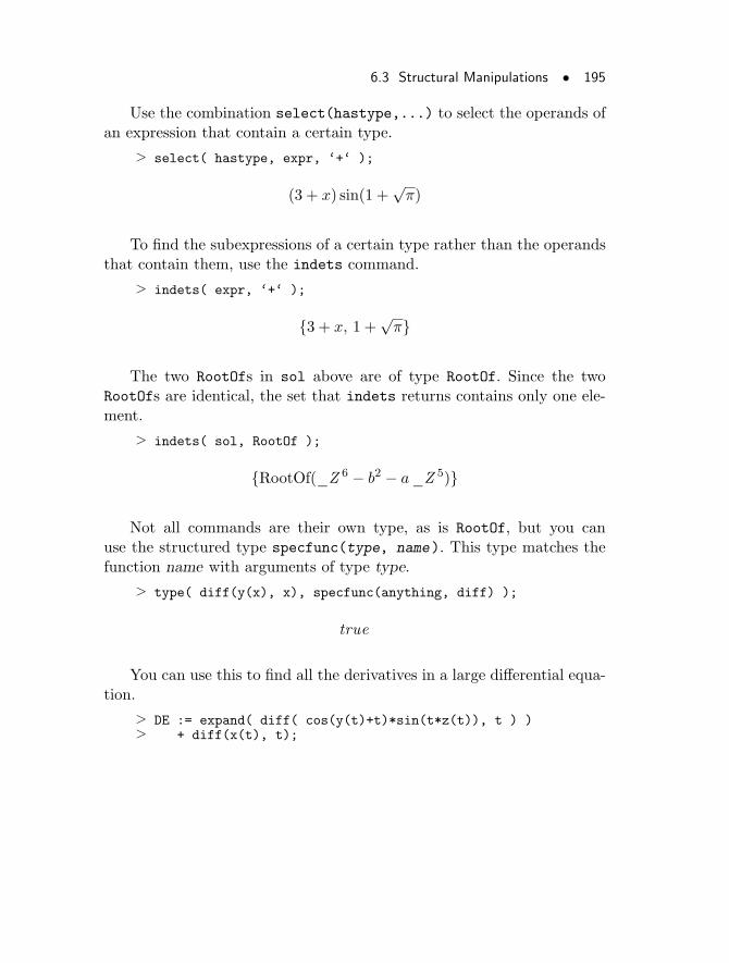
6.3 Structural Manipulations • 195
Use the combination select(hastype,...) to select the operands ofan expression that contain a certain type.
> select( hastype, expr, ‘+‘ );
(3 + x) sin(1 +√π)
To find the subexpressions of a certain type rather than the operandsthat contain them, use the indets command.
> indets( expr, ‘+‘ );
{3 + x, 1 +√π}
The two RootOfs in sol above are of type RootOf. Since the twoRootOfs are identical, the set that indets returns contains only one ele-ment.
> indets( sol, RootOf );
{RootOf(_Z 6 − b2 − a_Z 5)}
Not all commands are their own type, as is RootOf, but you canuse the structured type specfunc(type, name). This type matches thefunction name with arguments of type type.
> type( diff(y(x), x), specfunc(anything, diff) );
true
You can use this to find all the derivatives in a large differential equa-tion.
> DE := expand( diff( cos(y(t)+t)*sin(t*z(t)), t ) )> + diff(x(t), t);
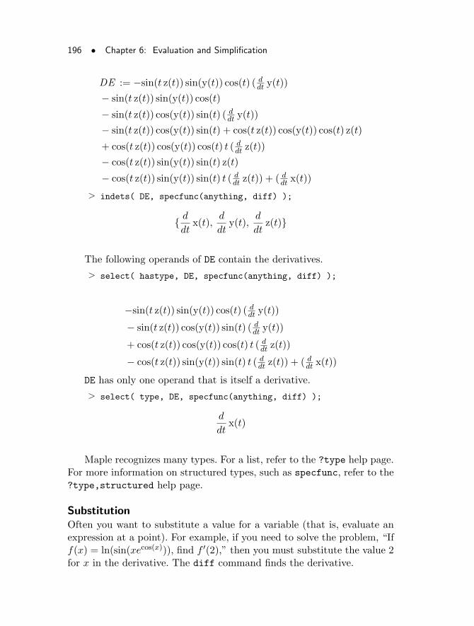
196 • Chapter 6: Evaluation and Simplification
DE := −sin(t z(t)) sin(y(t)) cos(t) ( ddt y(t))
− sin(t z(t)) sin(y(t)) cos(t)
− sin(t z(t)) cos(y(t)) sin(t) ( ddt y(t))
− sin(t z(t)) cos(y(t)) sin(t) + cos(t z(t)) cos(y(t)) cos(t) z(t)
+ cos(t z(t)) cos(y(t)) cos(t) t ( ddt z(t))
− cos(t z(t)) sin(y(t)) sin(t) z(t)
− cos(t z(t)) sin(y(t)) sin(t) t ( ddt z(t)) + ( d
dt x(t))
> indets( DE, specfunc(anything, diff) );
{ d
dtx(t),
d
dty(t),
d
dtz(t)}
The following operands of DE contain the derivatives.
> select( hastype, DE, specfunc(anything, diff) );
−sin(t z(t)) sin(y(t)) cos(t) ( ddt y(t))
− sin(t z(t)) cos(y(t)) sin(t) ( ddt y(t))
+ cos(t z(t)) cos(y(t)) cos(t) t ( ddt z(t))
− cos(t z(t)) sin(y(t)) sin(t) t ( ddt z(t)) + ( d
dt x(t))
DE has only one operand that is itself a derivative.
> select( type, DE, specfunc(anything, diff) );
d
dtx(t)
Maple recognizes many types. For a list, refer to the ?type help page.For more information on structured types, such as specfunc, refer to the?type,structured help page.
SubstitutionOften you want to substitute a value for a variable (that is, evaluate anexpression at a point). For example, if you need to solve the problem, “Iff(x) = ln(sin(xecos(x))), find f ′(2),” then you must substitute the value 2for x in the derivative. The diff command finds the derivative.
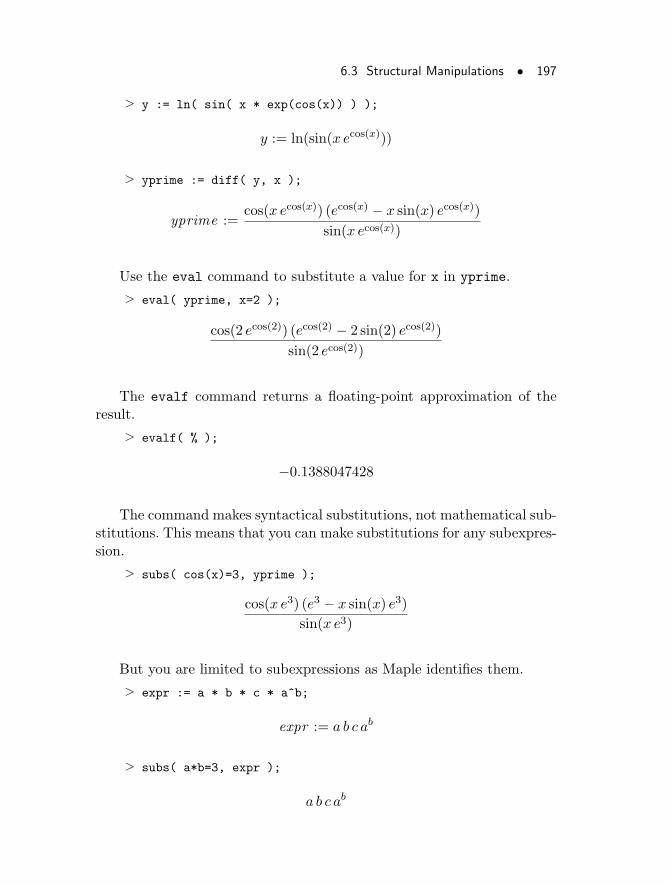
6.3 Structural Manipulations • 197
> y := ln( sin( x * exp(cos(x)) ) );
y := ln(sin(x ecos(x)))
> yprime := diff( y, x );
yprime :=cos(x ecos(x)) (ecos(x) − x sin(x) ecos(x))
sin(x ecos(x))
Use the eval command to substitute a value for x in yprime.
> eval( yprime, x=2 );
cos(2 ecos(2)) (ecos(2) − 2 sin(2) ecos(2))
sin(2 ecos(2))
The evalf command returns a floating-point approximation of theresult.
> evalf( % );
−0.1388047428
The command makes syntactical substitutions, not mathematical sub-stitutions. This means that you can make substitutions for any subexpres-sion.
> subs( cos(x)=3, yprime );
cos(x e3) (e3 − x sin(x) e3)
sin(x e3)
But you are limited to subexpressions as Maple identifies them.
> expr := a * b * c * a^b;
expr := a b c ab
> subs( a*b=3, expr );
a b c ab
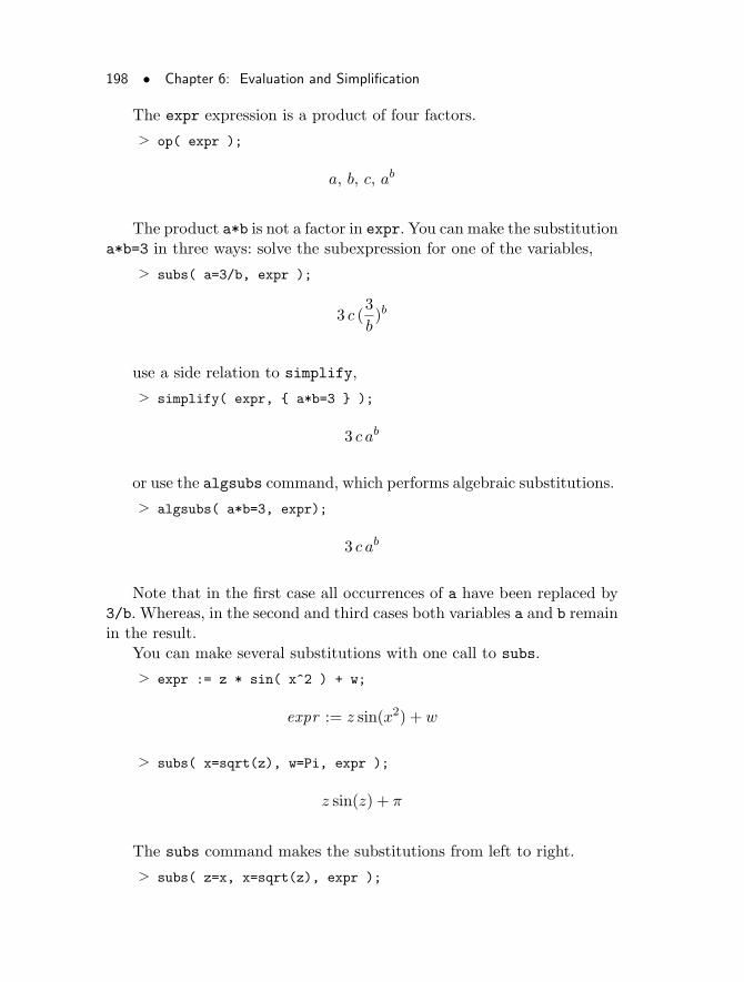
198 • Chapter 6: Evaluation and Simplification
The expr expression is a product of four factors.
> op( expr );
a, b, c, ab
The product a*b is not a factor in expr. You can make the substitutiona*b=3 in three ways: solve the subexpression for one of the variables,
> subs( a=3/b, expr );
3 c (3
b)b
use a side relation to simplify,
> simplify( expr, { a*b=3 } );
3 c ab
or use the algsubs command, which performs algebraic substitutions.
> algsubs( a*b=3, expr);
3 c ab
Note that in the first case all occurrences of a have been replaced by3/b. Whereas, in the second and third cases both variables a and b remainin the result.
You can make several substitutions with one call to subs.
> expr := z * sin( x^2 ) + w;
expr := z sin(x2) + w
> subs( x=sqrt(z), w=Pi, expr );
z sin(z) + π
The subs command makes the substitutions from left to right.
> subs( z=x, x=sqrt(z), expr );
6.3 Structural Manipulations • 199
√z sin(z) + w
If you give a set or list of substitutions, subsmakes those substitutionssimultaneously.
> subs( { x=sqrt(Pi), z=3 }, expr );
3 sin(π) + w
Note that in general you must explicitly evaluate the result of a callto subs.
> eval( % );
w
Use the subsop command to substitute for a specific operand of anexpression.
> expr := 5^x;
expr := 5x
> op( expr );
5, x
> subsop( 1=t, expr );
tx
The zeroth operand of a function is typically the name of the function.
> expr := cos(x);
expr := cos(x)
> subsop( 0=sin, expr );
sin(x)
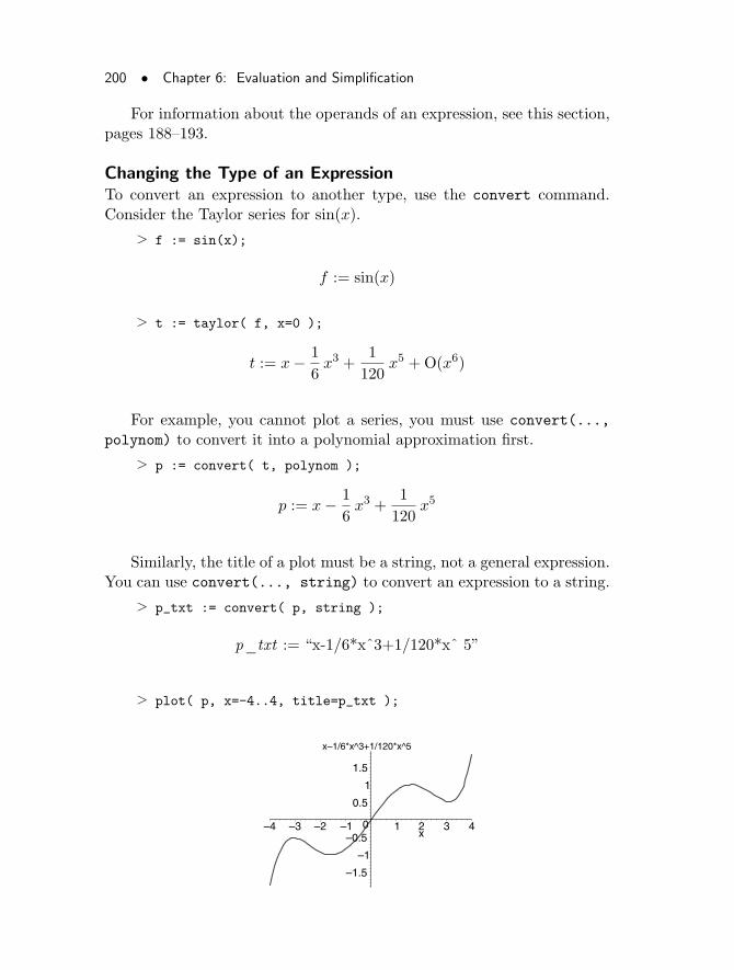
200 • Chapter 6: Evaluation and Simplification
For information about the operands of an expression, see this section,pages 188–193.
Changing the Type of an ExpressionTo convert an expression to another type, use the convert command.Consider the Taylor series for sin(x).
> f := sin(x);
f := sin(x)
> t := taylor( f, x=0 );
t := x− 1
6x3 +
1
120x5 +O(x6)
For example, you cannot plot a series, you must use convert(...,
polynom) to convert it into a polynomial approximation first.
> p := convert( t, polynom );
p := x− 1
6x3 +
1
120x5
Similarly, the title of a plot must be a string, not a general expression.You can use convert(..., string) to convert an expression to a string.
> p_txt := convert( p, string );
p_txt := “x-1/6*x^3+1/120*x^ 5”
> plot( p, x=-4..4, title=p_txt );
x–1/6*x^3+1/120*x^5
–1.5
–1
–0.50
0.5
1
1.5
–4 –3 –2 –1 1 2 3 4x
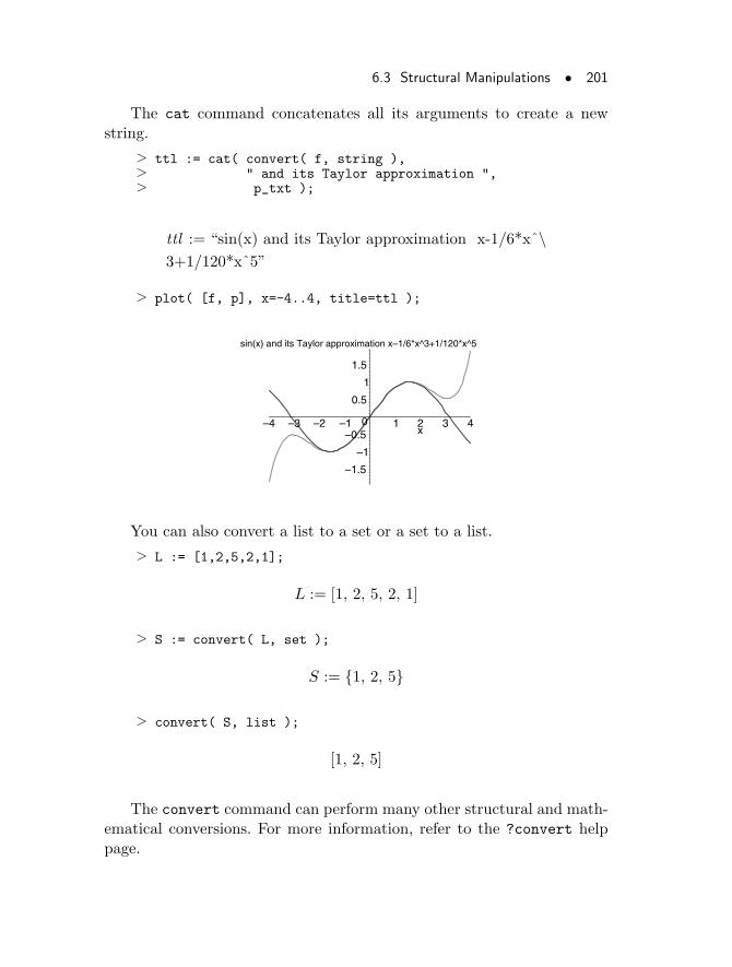
6.3 Structural Manipulations • 201
The cat command concatenates all its arguments to create a newstring.
> ttl := cat( convert( f, string ),> " and its Taylor approximation ",> p_txt );
ttl := “sin(x) and its Taylor approximation x-1/6*x^\3+1/120*x^5”
> plot( [f, p], x=-4..4, title=ttl );
sin(x) and its Taylor approximation x–1/6*x^3+1/120*x^5
–1.5
–1
–0.50
0.5
1
1.5
–4 –3 –2 –1 1 2 3 4x
You can also convert a list to a set or a set to a list.
> L := [1,2,5,2,1];
L := [1, 2, 5, 2, 1]
> S := convert( L, set );
S := {1, 2, 5}
> convert( S, list );
[1, 2, 5]
The convert command can perform many other structural and math-ematical conversions. For more information, refer to the ?convert helppage.
202 • Chapter 6: Evaluation and Simplification
6.4 Evaluation Rules
In a symbolic mathematics program such as Maple you encounter theissue of evaluation. If you assign the value y to x, the value z to y, andthe value 5 to z, then to what should x evaluate?
Levels of EvaluationMaple, in most cases, does full evaluation of names. That is, when you usea name or symbol, Maple checks if the name or symbol has an assignedvalue. If it has a value, Maple substitutes the value for the name. If thisvalue itself has an assigned value, Maple performs a substitution again,and so on, recursively, until no more substitutions are possible.
> x := y;
x := y
> y := z;
y := z
> z := 5;
z := 5
Maple evaluates x fully. That is, Maple substitutes y for x, z for y,and then 5 for z.
> x;
5
You can use the eval command to control the level of evaluation ofan expression. If you call eval with one argument, then eval evaluatesthat argument fully.
> eval(x);
5
A second argument to eval specifies how far you want to evaluate thefirst argument.
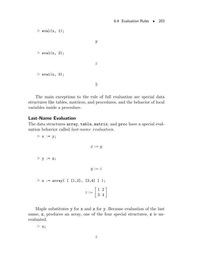
6.4 Evaluation Rules • 203
> eval(x, 1);
y
> eval(x, 2);
z
> eval(x, 3);
5
The main exceptions to the rule of full evaluation are special datastructures like tables, matrices, and procedures, and the behavior of localvariables inside a procedure.
Last-Name EvaluationThe data structures array, table, matrix, and proc have a special eval-uation behavior called last-name evaluation.
> x := y;
x := y
> y := z;
y := z
> z := array( [ [1,2], [3,4] ] );
z :=
[
1 23 4
]
Maple substitutes y for x and z for y. Because evaluation of the lastname, z, produces an array, one of the four special structures, z is un-evaluated.
> x;
z
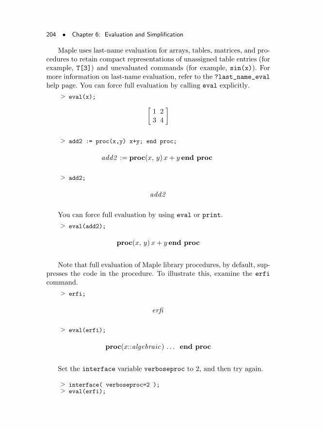
204 • Chapter 6: Evaluation and Simplification
Maple uses last-name evaluation for arrays, tables, matrices, and pro-cedures to retain compact representations of unassigned table entries (forexample, T[3]) and unevaluated commands (for example, sin(x)). Formore information on last-name evaluation, refer to the ?last_name_evalhelp page. You can force full evaluation by calling eval explicitly.
> eval(x);
[
1 23 4
]
> add2 := proc(x,y) x+y; end proc;
add2 := proc(x, y)x+ y end proc
> add2;
add2
You can force full evaluation by using eval or print.
> eval(add2);
proc(x, y)x+ y end proc
Note that full evaluation of Maple library procedures, by default, sup-presses the code in the procedure. To illustrate this, examine the erfi
command.
> erfi;
erfi
> eval(erfi);
proc(x::algebraic) . . . end proc
Set the interface variable verboseproc to 2, and then try again.
> interface( verboseproc=2 );> eval(erfi);
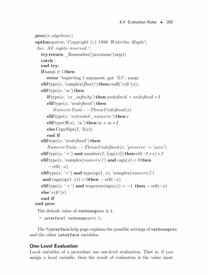
6.4 Evaluation Rules • 205
proc(x::algebraic)
optionsystem, ‘Copyright (c) 1996 Waterloo Maple\Inc . All rights reserved .‘;
try return _Remember(’procname’(args))
catch :end try;if nargs 6= 1 then
error “expecting 1 argument, got %1”, nargs
elif type(x, ’complex(float)’) then evalf(’erfi ’(x))
elif type(x, ’∞’) then
if type(x, ’cx_infinity ’) thenundefined + undefined ∗ Ielif type(x, ’undefined ’) then
NumericTools : −ThrowUndefined (x)
elif type(x, ’extended_numeric ’) thenx
elif type(<(x), ’∞’) then∞+∞∗ IelseCopySign(I, =(x))end if
elif type(x, ’undefined ’) then
NumericTools : −ThrowUndefined (x, ’preserve ’ = ’axes ’)
elif type(x, ‘ ∗ ‘) and member(I, {op(x)}) then erf(−I ∗ x) ∗ Ielif type(x, ’complex(numeric)’) and csgn(x) < 0 then
− erfi(−x)
eliftype(x, ‘ ∗ ‘) and type(op(1, x), ’complex(numeric)’)
and csgn(op(1, x)) < 0then − erfi(−x)
elif type(x, ‘ + ‘) and traperror(sign(x)) = −1 then − erfi(−x)
else ’erfi ’(x)
end ifend proc
The default value of verboseproc is 1.
> interface( verboseproc=1 );
The ?interface help page explains the possible settings of verboseprocand the other interface variables.
One-Level EvaluationLocal variables of a procedure use one-level evaluation. That is, if youassign a local variable, then the result of evaluation is the value most
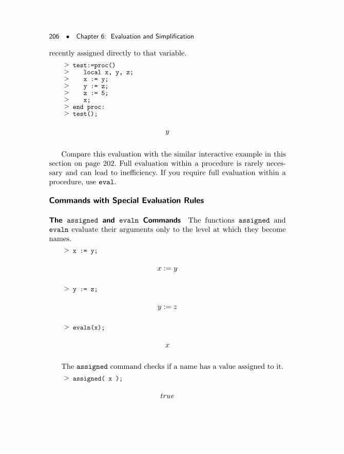
206 • Chapter 6: Evaluation and Simplification
recently assigned directly to that variable.
> test:=proc()> local x, y, z;> x := y;> y := z;> z := 5;> x;> end proc:> test();
y
Compare this evaluation with the similar interactive example in thissection on page 202. Full evaluation within a procedure is rarely neces-sary and can lead to inefficiency. If you require full evaluation within aprocedure, use eval.
Commands with Special Evaluation Rules
The assigned and evaln Commands The functions assigned andevaln evaluate their arguments only to the level at which they becomenames.
> x := y;
x := y
> y := z;
y := z
> evaln(x);
x
The assigned command checks if a name has a value assigned to it.
> assigned( x );
true
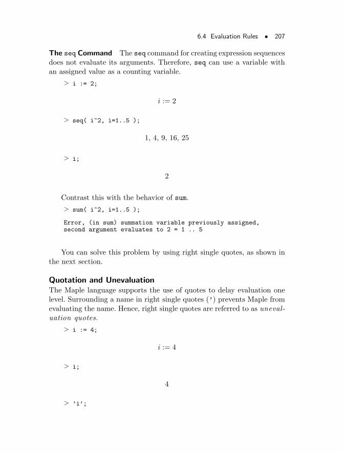
6.4 Evaluation Rules • 207
The seq Command The seq command for creating expression sequencesdoes not evaluate its arguments. Therefore, seq can use a variable withan assigned value as a counting variable.
> i := 2;
i := 2
> seq( i^2, i=1..5 );
1, 4, 9, 16, 25
> i;
2
Contrast this with the behavior of sum.
> sum( i^2, i=1..5 );
Error, (in sum) summation variable previously assigned,second argument evaluates to 2 = 1 .. 5
You can solve this problem by using right single quotes, as shown inthe next section.
Quotation and UnevaluationThe Maple language supports the use of quotes to delay evaluation onelevel. Surrounding a name in right single quotes (’) prevents Maple fromevaluating the name. Hence, right single quotes are referred to as uneval-uation quotes.
> i := 4;
i := 4
> i;
4
> ’i’;
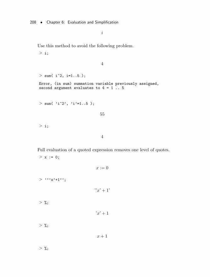
208 • Chapter 6: Evaluation and Simplification
i
Use this method to avoid the following problem.
> i;
4
> sum( i^2, i=1..5 );
Error, (in sum) summation variable previously assigned,second argument evaluates to 4 = 1 .. 5
> sum( ’i^2’, ’i’=1..5 );
55
> i;
4
Full evaluation of a quoted expression removes one level of quotes.
> x := 0;
x := 0
> ’’’x’+1’’;
’’x’ + 1’
> %;
’x’ + 1
> %;
x+ 1
> %;
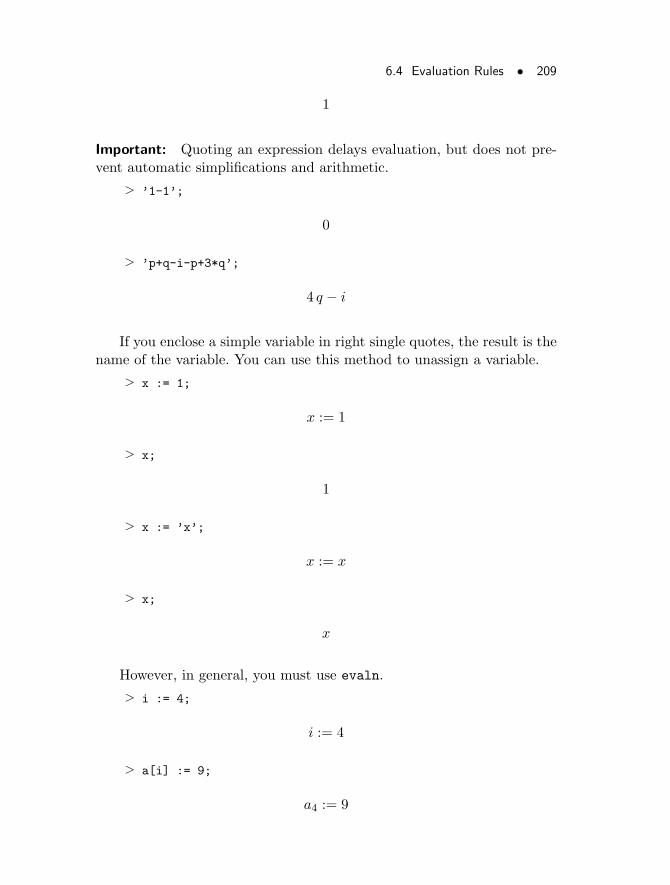
6.4 Evaluation Rules • 209
1
Important: Quoting an expression delays evaluation, but does not pre-vent automatic simplifications and arithmetic.
> ’1-1’;
0
> ’p+q-i-p+3*q’;
4 q − i
If you enclose a simple variable in right single quotes, the result is thename of the variable. You can use this method to unassign a variable.
> x := 1;
x := 1
> x;
1
> x := ’x’;
x := x
> x;
x
However, in general, you must use evaln.
> i := 4;
i := 4
> a[i] := 9;
a4 := 9
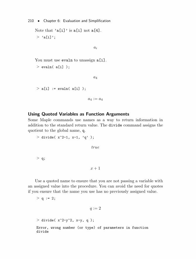
210 • Chapter 6: Evaluation and Simplification
Note that ’a[i]’ is a[i] not a[4].
> ’a[i]’;
ai
You must use evaln to unassign a[i].
> evaln( a[i] );
a4
> a[i] := evaln( a[i] );
a4 := a4
Using Quoted Variables as Function ArgumentsSome Maple commands use names as a way to return information inaddition to the standard return value. The divide command assigns thequotient to the global name, q.
> divide( x^2-1, x-1, ’q’ );
true
> q;
x+ 1
Use a quoted name to ensure that you are not passing a variable withan assigned value into the procedure. You can avoid the need for quotesif you ensure that the name you use has no previously assigned value.
> q := 2;
q := 2
> divide( x^2-y^2, x-y, q );
Error, wrong number (or type) of parameters in functiondivide
6.4 Evaluation Rules • 211
> q := evaln(q);
q := q
> divide( x^2-y^2, x-y, q );
true
> q;
x+ y
Note: The rem, quo, irem, and iquo commands behave in a similarmanner.
Concatenation of NamesConcatenation is a way to form new variable names based on others.
> a||b;
ab
The concatenation operator, “||”, in a name causes evaluation of theright-hand side of the operator, but not the left.
> a := x;
a := x
> b := 2;
b := 2
> a||b;
a2
> c := 3;
212 • Chapter 6: Evaluation and Simplification
c := 3
> a||b||c;
a23
If a name does not evaluate to a single symbol, Maple does not eval-uate a concatenation.
> a := x;
a := x
> b := y+1;
b := y + 1
> new_name := a||b;
new_name := a||(y + 1)
> y := 3;
y := 3
> new_name;
a4
You can use concatenated names to assign and create expressions.
> i := 1;
i := 1
> b||i := 0;
b1 := 0
You must use right single quotes.
6.5 Conclusion • 213
> sum( ’a||k’ * x^k, k=0..8 );
a0 + a1 x+ a2 x2 + a3 x3 + a4 x4 + a5 x5 + a6 x6 + a7 x7
+ a8 x8
If you do not use right single quotes, Maple evaluates a||k to ak.
> sum( a||k * x^k, k=0..8 );
ak + ak x+ ak x2 + ak x3 + ak x4 + ak x5 + ak x6 + ak x7
+ ak x8
You can also use concatenation to form title strings for plots.
6.5 Conclusion
In this chapter, you have seen how to perform many kinds of expressionmanipulations, from adding two equations to selecting individual parts ofa general expression. In general, no rule specifies which form of an expres-sion is the simplest. The commands in this chapter allow you to convertan expression to many forms, often the ones you would consider simplest.If not, you can use side relations to specify your own simplification rules,or assumptions to specify properties of unknowns.
You have also seen that Maple, in most cases, uses full evaluationof variables. Some exceptions exist, which include last-name evaluationfor certain data structures, one-level evaluation for local variables in aprocedure, and delayed evaluation for names in right single quotes.

214 • Chapter 6: Evaluation and Simplification
7 Solving Calculus Problems
This chapter provides examples of how Maple can help you present andsolve problems from calculus.
In This Chapter• Introductory Calculus
• Ordinary Differential Equations
• Partial Differential Equations
7.1 Introductory Calculus
This section contains examples of how to illustrate ideas and solve prob-lems from calculus. The Student[Calculus1] package contains manycommands that are especially useful in this area.
The DerivativeThis section illustrates the graphical meaning of the derivative: the slopeof the tangent line. Then it shows you how to find the set of inflectionpoints for a function.
Define the function f :x 7→ exp(sin(x)) in the following manner.
> f := x -> exp( sin(x) );
f := x → esin(x)
Find the derivative of f evaluated at x0 = 1.
> x0 := 1;
215
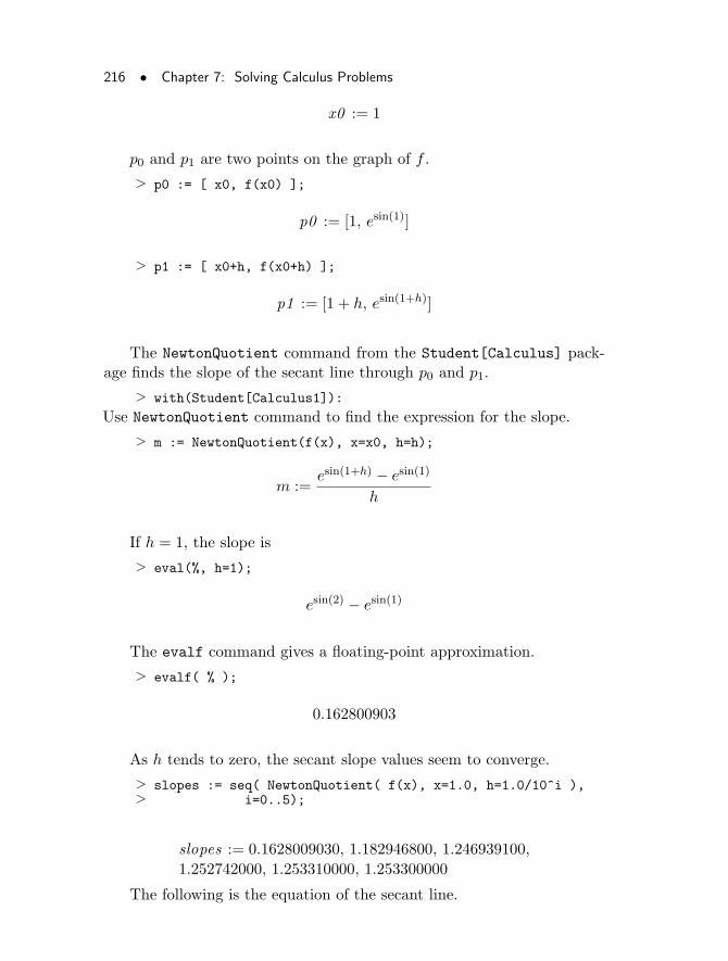
216 • Chapter 7: Solving Calculus Problems
x0 := 1
p0 and p1 are two points on the graph of f .
> p0 := [ x0, f(x0) ];
p0 := [1, esin(1)]
> p1 := [ x0+h, f(x0+h) ];
p1 := [1 + h, esin(1+h)]
The NewtonQuotient command from the Student[Calculus] pack-age finds the slope of the secant line through p0 and p1.
> with(Student[Calculus1]):
Use NewtonQuotient command to find the expression for the slope.
> m := NewtonQuotient(f(x), x=x0, h=h);
m :=esin(1+h) − esin(1)
h
If h = 1, the slope is
> eval(%, h=1);
esin(2) − esin(1)
The evalf command gives a floating-point approximation.
> evalf( % );
0.162800903
As h tends to zero, the secant slope values seem to converge.
> slopes := seq( NewtonQuotient( f(x), x=1.0, h=1.0/10^i ),> i=0..5);
slopes := 0.1628009030, 1.182946800, 1.246939100,
1.252742000, 1.253310000, 1.253300000
The following is the equation of the secant line.
7.1 Introductory Calculus • 217
> y - p0[2] = m * ( x - p0[1] );
y − esin(1) =(esin(1+h) − esin(1)) (x− 1)
h
The isolate command converts the equation to slope–intercept form.
> isolate( %, y );
y =(esin(1+h) − esin(1)) (x− 1)
h+ esin(1)
You must convert the equation to a function.
> secant := unapply( rhs(%), x );
secant := x → (esin(1+h) − esin(1)) (x− 1)
h+ esin(1)
You can now plot the secant and the function for different values ofh. First, make a sequence of plots.
> S := seq( plot( [f(x), secant(x)], x=0..4,> view=[0..4, 0..4] ),> h=[1.0, 0.1, .01, .001, .0001, .00001] ):
The display command from the plots package can display the plotsin sequence, that is, as an animation.
> with(plots):
Warning, the name changecoords has been redefined
> display( S, insequence=true, view=[0..4, 0..4] );
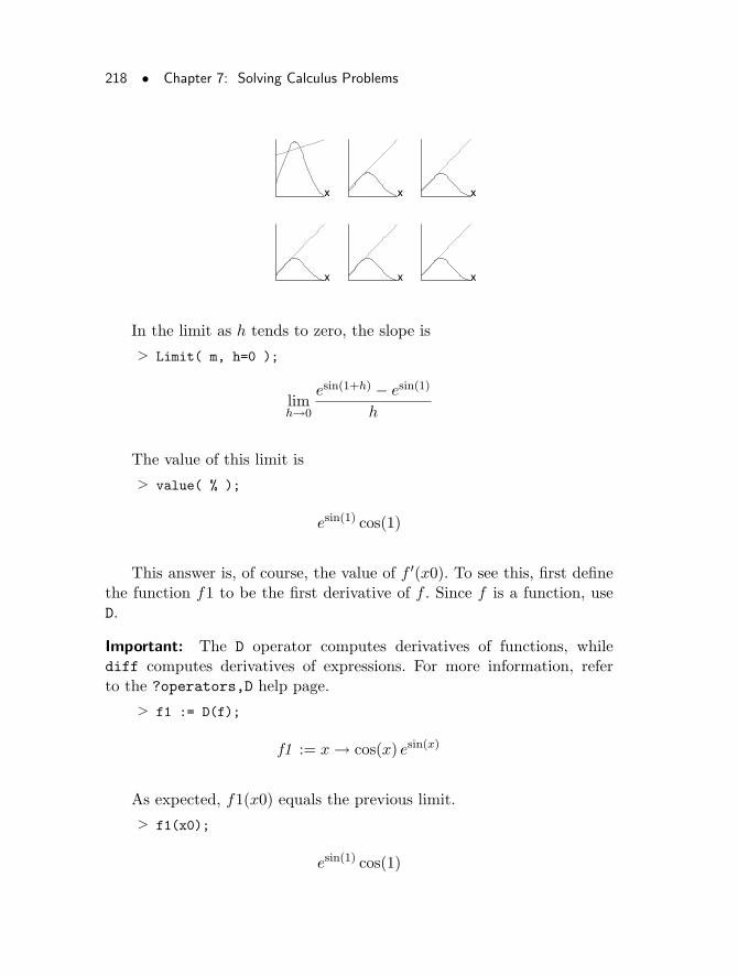
218 • Chapter 7: Solving Calculus Problems
xxx
xxx
In the limit as h tends to zero, the slope is
> Limit( m, h=0 );
limh→0
esin(1+h) − esin(1)
h
The value of this limit is
> value( % );
esin(1) cos(1)
This answer is, of course, the value of f ′(x0). To see this, first definethe function f1 to be the first derivative of f . Since f is a function, useD.
Important: The D operator computes derivatives of functions, whilediff computes derivatives of expressions. For more information, referto the ?operators,D help page.
> f1 := D(f);
f1 := x → cos(x) esin(x)
As expected, f1(x0) equals the previous limit.
> f1(x0);
esin(1) cos(1)
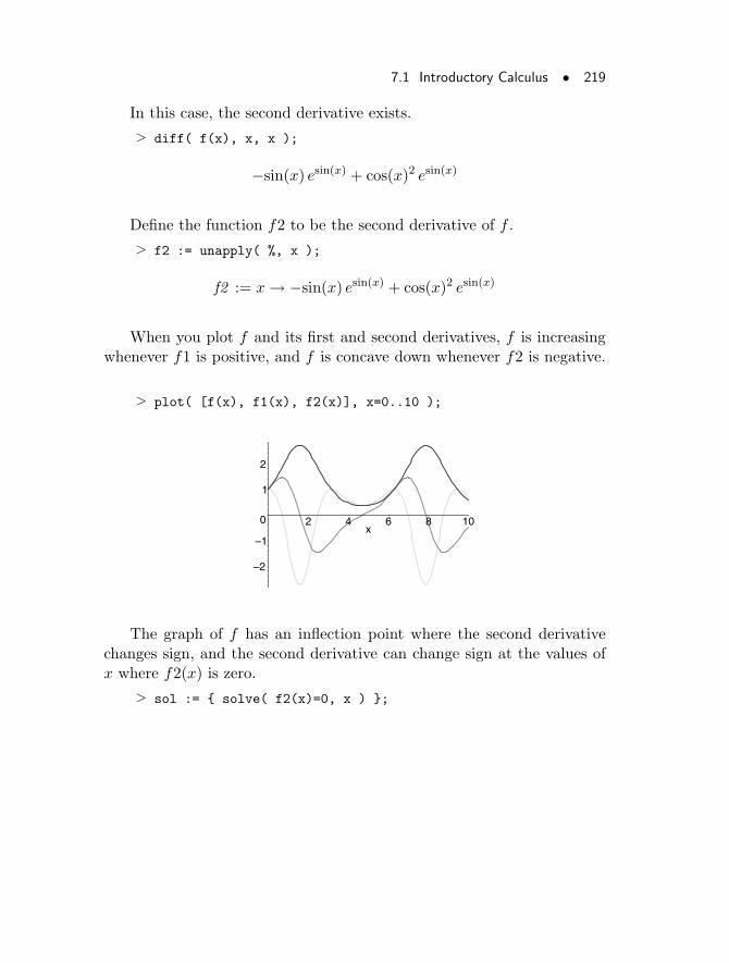
7.1 Introductory Calculus • 219
In this case, the second derivative exists.
> diff( f(x), x, x );
−sin(x) esin(x) + cos(x)2 esin(x)
Define the function f2 to be the second derivative of f .
> f2 := unapply( %, x );
f2 := x → −sin(x) esin(x) + cos(x)2 esin(x)
When you plot f and its first and second derivatives, f is increasingwhenever f1 is positive, and f is concave down whenever f2 is negative.
> plot( [f(x), f1(x), f2(x)], x=0..10 );
–2
–1
0
1
2
2 4 6 8 10x
The graph of f has an inflection point where the second derivativechanges sign, and the second derivative can change sign at the values ofx where f2(x) is zero.
> sol := { solve( f2(x)=0, x ) };
220 • Chapter 7: Solving Calculus Problems
sol :=
{
arctan
2
1
2
√5− 1
2√
−2 + 2√5
, −arctan
2
1
2
√5− 1
2√
−2 + 2√5
+ π,
arctan(−1
2
√5− 1
2,1
2
√
−2− 2√5),
arctan(−1
2
√5− 1
2, −1
2
√
−2− 2√5)
}
Two of these solutions are complex.
> evalf( sol );
{0.6662394321, 2.475353222,−1.570796327 + 1.061275064 I,
−1.570796327− 1.061275064 I}In this example, only the real solutions are of interest. Use the select
command to select the real constants from the solution set.
> infl := select( type, sol, realcons );
infl :=
arctan
2
1
2
√5− 1
2√
−2 + 2√5
, −arctan
2
1
2
√5− 1
2√
−2 + 2√5
+ π
> evalf( infl );
{0.6662394321, 2.475353222}
Observe that f2 actually does change sign at these x-values. The setof inflection points is given by the following.
> { seq( [x, f(x)], x=infl ) };
7.1 Introductory Calculus • 221
arctan
2
1
2
√5− 1
2√
−2 + 2√5
, e
2 1/2√5−1/2
√−2+2
√5
√
1+4(1/2
√5−1/2)2
−2+2√5
,
−arctan
2
1
2
√5− 1
2√
−2 + 2√5
+ π, e
2 1/2√5−1/2
√−2+2
√5
√
1+4(1/2
√5−1/2)2
−2+2√5
> evalf( % );
{[0.6662394321, 1.855276958],[2.475353222, 1.855276958]}
Since f is periodic, it has, of course, infinitely many inflection points.You can obtain these by shifting the two inflection points above horizon-tally by integer multiples of 2π.
A Taylor ApproximationThis section illustrates how you can use Maple to analyze the error termin a Taylor approximation. The following is Taylor’s formula.
> taylor( f(x), x=a );
f(a) + D(f)(a) (x− a) +1
2(D(2))(f)(a) (x− a)2 +
1
6(D(3))(f)(a)
(x− a)3 +1
24(D(4))(f)(a) (x− a)4 +
1
120(D(5))(f)(a) (x− a)5+
O((x− a)6)
You can use it to find a polynomial approximation of a function fnear x = a.
> f := x -> exp( sin(x) );
f := x → esin(x)
> a := Pi;
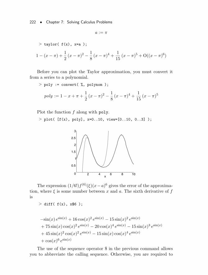
222 • Chapter 7: Solving Calculus Problems
a := π
> taylor( f(x), x=a );
1− (x− π) +1
2(x− π)2 − 1
8(x− π)4 +
1
15(x− π)5 +O((x− π)6)
Before you can plot the Taylor approximation, you must convert itfrom a series to a polynomial.
> poly := convert( %, polynom );
poly := 1− x+ π +1
2(x− π)2 − 1
8(x− π)4 +
1
15(x− π)5
Plot the function f along with poly.
> plot( [f(x), poly], x=0..10, view=[0..10, 0..3] );
0
0.5
1
1.5
2
2.5
3
2 4 6 8 10x
The expression (1/6!)f (6)(ξ)(x−a)6 gives the error of the approxima-tion, where ξ is some number between x and a. The sixth derivative of fis
> diff( f(x), x$6 );
−sin(x) esin(x) + 16 cos(x)2 esin(x) − 15 sin(x)2 esin(x)
+ 75 sin(x) cos(x)2 esin(x) − 20 cos(x)4 esin(x) − 15 sin(x)3 esin(x)
+ 45 sin(x)2 cos(x)2 esin(x) − 15 sin(x) cos(x)4 esin(x)
+ cos(x)6 esin(x)
The use of the sequence operator $ in the previous command allowsyou to abbreviate the calling sequence. Otherwise, you are required to
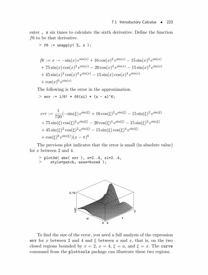
7.1 Introductory Calculus • 223
enter , x six times to calculate the sixth derivative. Define the functionf6 to be that derivative.
> f6 := unapply( %, x );
f6 := x → −sin(x) esin(x) + 16 cos(x)2 esin(x) − 15 sin(x)2 esin(x)
+ 75 sin(x) cos(x)2 esin(x) − 20 cos(x)4 esin(x) − 15 sin(x)3 esin(x)
+ 45 sin(x)2 cos(x)2 esin(x) − 15 sin(x) cos(x)4 esin(x)
+ cos(x)6 esin(x)
The following is the error in the approximation.
> err := 1/6! * f6(xi) * (x - a)^6;
err :=1
720(−sin(ξ) esin(ξ) + 16 cos(ξ)2 esin(ξ) − 15 sin(ξ)2 esin(ξ)
+ 75 sin(ξ) cos(ξ)2 esin(ξ) − 20 cos(ξ)4 esin(ξ) − 15 sin(ξ)3 esin(ξ)
+ 45 sin(ξ)2 cos(ξ)2 esin(ξ) − 15 sin(ξ) cos(ξ)4 esin(ξ)
+ cos(ξ)6 esin(ξ))(x− π)6
The previous plot indicates that the error is small (in absolute value)for x between 2 and 4.
> plot3d( abs( err ), x=2..4, xi=2..4,> style=patch, axes=boxed );
2
4
x
2
4xi
0
0.16
To find the size of the error, you need a full analysis of the expressionerr for x between 2 and 4 and ξ between a and x, that is, on the twoclosed regions bounded by x = 2, x = 4, ξ = a, and ξ = x. The curve
command from the plottools package can illustrate these two regions.
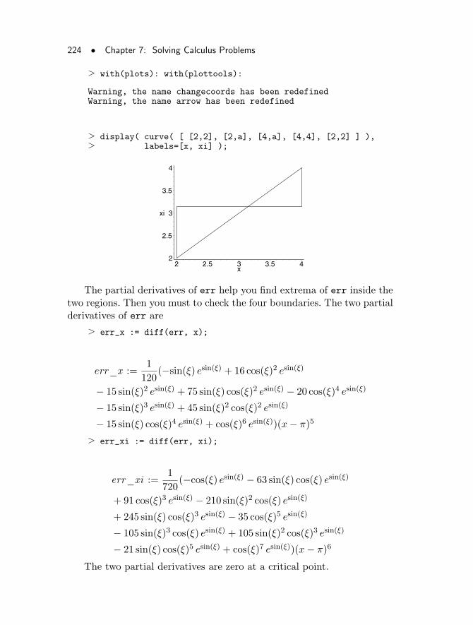
224 • Chapter 7: Solving Calculus Problems
> with(plots): with(plottools):
Warning, the name changecoords has been redefinedWarning, the name arrow has been redefined
> display( curve( [ [2,2], [2,a], [4,a], [4,4], [2,2] ] ),> labels=[x, xi] );
2
2.5
3
3.5
4
xi
2 2.5 3 3.5 4x
The partial derivatives of err help you find extrema of err inside thetwo regions. Then you must to check the four boundaries. The two partialderivatives of err are
> err_x := diff(err, x);
err_x :=1
120(−sin(ξ) esin(ξ) + 16 cos(ξ)2 esin(ξ)
− 15 sin(ξ)2 esin(ξ) + 75 sin(ξ) cos(ξ)2 esin(ξ) − 20 cos(ξ)4 esin(ξ)
− 15 sin(ξ)3 esin(ξ) + 45 sin(ξ)2 cos(ξ)2 esin(ξ)
− 15 sin(ξ) cos(ξ)4 esin(ξ) + cos(ξ)6 esin(ξ))(x− π)5
> err_xi := diff(err, xi);
err_xi :=1
720(−cos(ξ) esin(ξ) − 63 sin(ξ) cos(ξ) esin(ξ)
+ 91 cos(ξ)3 esin(ξ) − 210 sin(ξ)2 cos(ξ) esin(ξ)
+ 245 sin(ξ) cos(ξ)3 esin(ξ) − 35 cos(ξ)5 esin(ξ)
− 105 sin(ξ)3 cos(ξ) esin(ξ) + 105 sin(ξ)2 cos(ξ)3 esin(ξ)
− 21 sin(ξ) cos(ξ)5 esin(ξ) + cos(ξ)7 esin(ξ))(x− π)6
The two partial derivatives are zero at a critical point.
7.1 Introductory Calculus • 225
> sol := solve( {err_x=0, err_xi=0}, {x, xi} );
sol := {ξ = ξ, x = π}
The error is zero at this critical point.
> eval( err, sol );
0
Collect a set of critical values. The largest critical value then boundsthe maximal error.
> critical := { % };
critical := {0}
The partial derivative err_xi is zero at a critical point on either ofthe two boundaries at x = 2 and x = 4.
> sol := { solve( err_xi=0, xi ) };
sol := {arctan(RootOf(%1, index = 2),
RootOf(_Z 2 +RootOf(%1, index = 2)2 − 1)), arctan(
RootOf(%1, index = 5),
RootOf(_Z 2 +RootOf(%1, index = 5)2 − 1)), arctan(
RootOf(%1, index = 6),
RootOf(_Z 2 +RootOf(%1, index = 6)2 − 1)), arctan(
RootOf(%1, index = 1),
RootOf(_Z 2 +RootOf(%1, index = 1)2 − 1)), arctan(
RootOf(%1, index = 4),
RootOf(_Z 2 +RootOf(%1, index = 4)2 − 1)), arctan(
RootOf(%1, index = 3),
RootOf(_Z 2 +RootOf(%1, index = 3)2 − 1)),1
2π}
%1 := −56− 161_Z + 129_Z 2 + 308_Z 3 + 137_Z 4
+ 21_Z 5 +_Z 6
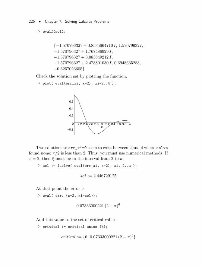
226 • Chapter 7: Solving Calculus Problems
> evalf(sol);
{−1.570796327 + 0.8535664710 I, 1.570796327,
−1.570796327 + 1.767486929 I,
−1.570796327 + 3.083849212 I,
−1.570796327 + 2.473801030 I, 0.6948635283,
−0.3257026605}Check the solution set by plotting the function.
> plot( eval(err_xi, x=2), xi=2..4 );
–0.2
0
0.2
0.4
0.6
2.2 2.4 2.6 2.8 3 3.2 3.4 3.6 3.8 4xi
Two solutions to err_xi=0 seem to exist between 2 and 4 where solvefound none: π/2 is less than 2. Thus, you must use numerical methods. Ifx = 2, then ξ must be in the interval from 2 to a.
> sol := fsolve( eval(err_xi, x=2), xi, 2..a );
sol := 2.446729125
At that point the error is
> eval( err, {x=2, xi=sol});
0.07333000221 (2− π)6
Add this value to the set of critical values.
> critical := critical union {%};
critical := {0, 0.07333000221 (2− π)6}
7.1 Introductory Calculus • 227
If x = 4 then ξ must be between a and 4.
> sol := fsolve( eval(err_xi, x=4), xi, a..4 );
sol := 3.467295314
At that point, the error is
> eval( err, {x=4, xi=sol} );
−0.01542298119 (4− π)6
> critical := critical union {%};
critical :={0, 0.07333000221 (2− π)6, −0.01542298119 (4− π)6}
At the ξ = a boundary, the error is
> B := eval( err, xi=a );
B := − 1
240(x− π)6
The derivative, B1, of B is zero at a critical point.
> B1 := diff( B, x );
B1 := − 1
40(x− π)5
> sol := { solve( B1=0, x ) };
sol := {π}
At the critical point the error is
> eval( B, x=sol[1] );
0
> critical := critical union { % };
228 • Chapter 7: Solving Calculus Problems
critical :={0, 0.07333000221 (2− π)6, −0.01542298119 (4− π)6}
At the last boundary, ξ = x, the error is
> B := eval( err, xi=x );
B :=1
720(−sin(x) esin(x) + 16 cos(x)2 esin(x) − 15 sin(x)2 esin(x)
+ 75 sin(x) cos(x)2 esin(x) − 20 cos(x)4 esin(x) − 15 sin(x)3 esin(x)
+ 45 sin(x)2 cos(x)2 esin(x) − 15 sin(x) cos(x)4 esin(x)
+ cos(x)6 esin(x))(x− π)6
Again, find where the derivative is zero.
> B1 := diff( B, x );
B1 :=1
720(−cos(x) esin(x) − 63 sin(x) cos(x) esin(x)
+ 91 cos(x)3 esin(x) − 210 sin(x)2 cos(x) esin(x)
+ 245 sin(x) cos(x)3 esin(x) − 35 cos(x)5 esin(x)
− 105 sin(x)3 cos(x) esin(x) + 105 sin(x)2 cos(x)3 esin(x)
− 21 sin(x) cos(x)5 esin(x) + cos(x)7 esin(x))(x− π)6 +1
120(
−sin(x) esin(x) + 16 cos(x)2 esin(x) − 15 sin(x)2 esin(x)
+ 75 sin(x) cos(x)2 esin(x) − 20 cos(x)4 esin(x) − 15 sin(x)3 esin(x)
+ 45 sin(x)2 cos(x)2 esin(x) − 15 sin(x) cos(x)4 esin(x)
+ cos(x)6 esin(x))(x− π)5
> sol := { solve( B1=0, x ) };
sol := {π}
Check the solution by plotting.
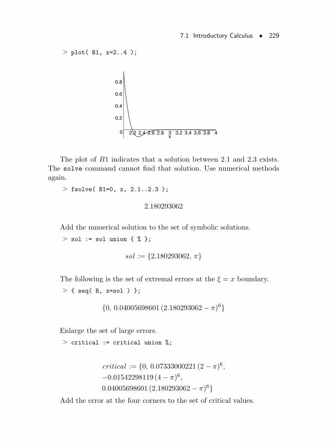
7.1 Introductory Calculus • 229
> plot( B1, x=2..4 );
0
0.2
0.4
0.6
0.8
2.2 2.4 2.6 2.8 3 3.2 3.4 3.6 3.8 4x
The plot of B1 indicates that a solution between 2.1 and 2.3 exists.The solve command cannot find that solution. Use numerical methodsagain.
> fsolve( B1=0, x, 2.1..2.3 );
2.180293062
Add the numerical solution to the set of symbolic solutions.
> sol := sol union { % };
sol := {2.180293062, π}
The following is the set of extremal errors at the ξ = x boundary.
> { seq( B, x=sol ) };
{0, 0.04005698601 (2.180293062− π)6}
Enlarge the set of large errors.
> critical := critical union %;
critical := {0, 0.07333000221 (2− π)6,
−0.01542298119 (4− π)6,
0.04005698601 (2.180293062− π)6}Add the error at the four corners to the set of critical values.
230 • Chapter 7: Solving Calculus Problems
> critical := critical union> { eval( err, {xi=2, x=2} ),> eval( err, {xi=2, x=4} ),> eval( err, {xi=4, x=2} ),> eval( err, {xi=4, x=4} ) };
critical := {0, 0.07333000221 (2− π)6,1
720(−sin(4) esin(4)
+ 16 cos(4)2 esin(4) − 15 sin(4)2 esin(4) + 75 sin(4) cos(4)2 esin(4)
− 20 cos(4)4 esin(4) − 15 sin(4)3 esin(4)
+ 45 sin(4)2 cos(4)2 esin(4) − 15 sin(4) cos(4)4 esin(4)
+ cos(4)6 esin(4))(2− π)6,1
720(−sin(2) esin(2)
+ 16 cos(2)2 esin(2) − 15 sin(2)2 esin(2) + 75 sin(2) cos(2)2 esin(2)
− 20 cos(2)4 esin(2) − 15 sin(2)3 esin(2)
+ 45 sin(2)2 cos(2)2 esin(2) − 15 sin(2) cos(2)4 esin(2)
+ cos(2)6 esin(2))(4− π)6, −0.01542298119 (4− π)6,
0.04005698601 (2.180293062− π)6,1
720(−sin(4) esin(4)
+ 16 cos(4)2 esin(4) − 15 sin(4)2 esin(4) + 75 sin(4) cos(4)2 esin(4)
− 20 cos(4)4 esin(4) − 15 sin(4)3 esin(4)
+ 45 sin(4)2 cos(4)2 esin(4) − 15 sin(4) cos(4)4 esin(4)
+ cos(4)6 esin(4))(4− π)6,1
720(−sin(2) esin(2)
+ 16 cos(2)2 esin(2) − 15 sin(2)2 esin(2) + 75 sin(2) cos(2)2 esin(2)
− 20 cos(2)4 esin(2) − 15 sin(2)3 esin(2)
+ 45 sin(2)2 cos(2)2 esin(2) − 15 sin(2) cos(2)4 esin(2)
+ cos(2)6 esin(2))(2− π)6}Find the maximum of the absolute values of the elements of critical.
First, map the abs command onto the elements of critical.
> map( abs, critical );
7.1 Introductory Calculus • 231
{0, 0.07333000221 (2− π)6,− 1
720(−sin(4) esin(4)
+ 16 cos(4)2 esin(4) − 15 sin(4)2 esin(4) + 75 sin(4) cos(4)2 esin(4)
− 20 cos(4)4 esin(4) − 15 sin(4)3 esin(4)
+ 45 sin(4)2 cos(4)2 esin(4) − 15 sin(4) cos(4)4 esin(4)
+ cos(4)6 esin(4))(2− π)6,− 1
720(−sin(2) esin(2)
+ 16 cos(2)2 esin(2) − 15 sin(2)2 esin(2) + 75 sin(2) cos(2)2 esin(2)
− 20 cos(2)4 esin(2) − 15 sin(2)3 esin(2)
+ 45 sin(2)2 cos(2)2 esin(2) − 15 sin(2) cos(2)4 esin(2)
+ cos(2)6 esin(2))(4− π)6, 0.01542298119 (4− π)6,− 1
720(
−sin(2) esin(2) + 16 cos(2)2 esin(2) − 15 sin(2)2 esin(2)
+ 75 sin(2) cos(2)2 esin(2) − 20 cos(2)4 esin(2) − 15 sin(2)3 esin(2)
+ 45 sin(2)2 cos(2)2 esin(2) − 15 sin(2) cos(2)4 esin(2)
+ cos(2)6 esin(2))(2− π)6,− 1
720(−sin(4) esin(4)
+ 16 cos(4)2 esin(4) − 15 sin(4)2 esin(4) + 75 sin(4) cos(4)2 esin(4)
− 20 cos(4)4 esin(4) − 15 sin(4)3 esin(4)
+ 45 sin(4)2 cos(4)2 esin(4) − 15 sin(4) cos(4)4 esin(4)
+ cos(4)6 esin(4))(4− π)6,
0.04005698601 (2.180293062− π)6}Find the maximal element. The max command expects a sequence of
numbers, so you must use the op command to convert the set of valuesinto a sequence.
> max_error := max( op(%) );
max_error := 0.07333000221 (2− π)6
Approximately, this number is
> evalf( max_error );
0.1623112756
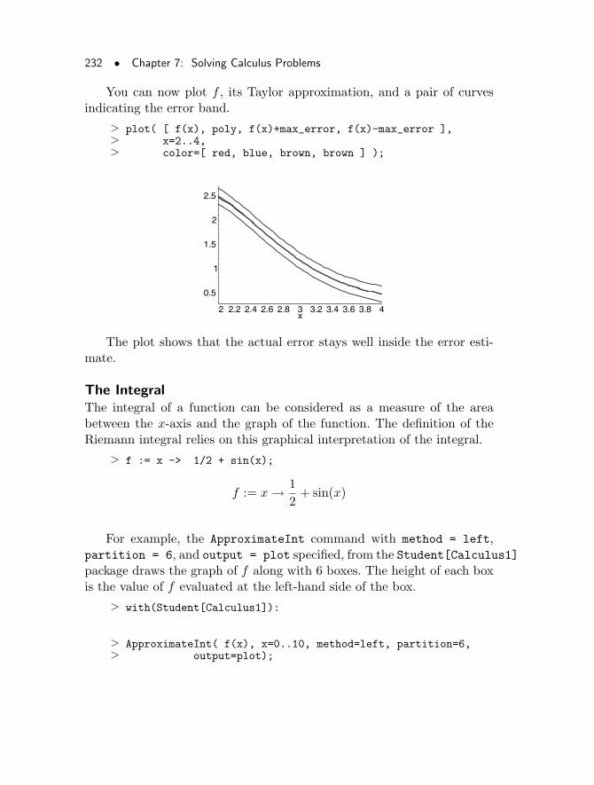
232 • Chapter 7: Solving Calculus Problems
You can now plot f , its Taylor approximation, and a pair of curvesindicating the error band.
> plot( [ f(x), poly, f(x)+max_error, f(x)-max_error ],> x=2..4,> color=[ red, blue, brown, brown ] );
0.5
1
1.5
2
2.5
2 2.2 2.4 2.6 2.8 3 3.2 3.4 3.6 3.8 4x
The plot shows that the actual error stays well inside the error esti-mate.
The IntegralThe integral of a function can be considered as a measure of the areabetween the x-axis and the graph of the function. The definition of theRiemann integral relies on this graphical interpretation of the integral.
> f := x -> 1/2 + sin(x);
f := x → 1
2+ sin(x)
For example, the ApproximateInt command with method = left,partition = 6, and output = plot specified, from the Student[Calculus1]package draws the graph of f along with 6 boxes. The height of each boxis the value of f evaluated at the left-hand side of the box.
> with(Student[Calculus1]):
> ApproximateInt( f(x), x=0..10, method=left, partition=6,> output=plot);
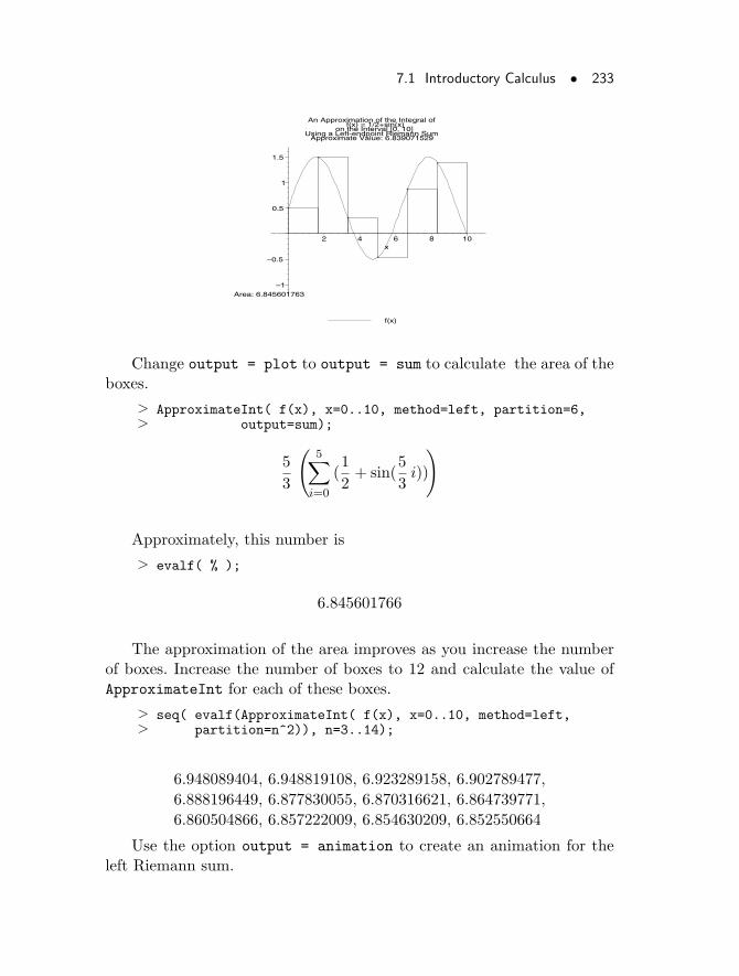
7.1 Introductory Calculus • 233
f(x)
An Approximation of the Integral off(x) = 1/2+sin(x)
on the Interval [0, 10]Using a Left-endpoint Riemann Sum
Approximate Value: 6.839071529
Area: 6.845601763
–1
–0.5
0.5
1
1.5
2 4 6 8 10x
Change output = plot to output = sum to calculate the area of theboxes.
> ApproximateInt( f(x), x=0..10, method=left, partition=6,> output=sum);
5
3
(
5∑
i=0
(1
2+ sin(
5
3i))
)
Approximately, this number is
> evalf( % );
6.845601766
The approximation of the area improves as you increase the numberof boxes. Increase the number of boxes to 12 and calculate the value ofApproximateInt for each of these boxes.
> seq( evalf(ApproximateInt( f(x), x=0..10, method=left,> partition=n^2)), n=3..14);
6.948089404, 6.948819108, 6.923289158, 6.902789477,
6.888196449, 6.877830055, 6.870316621, 6.864739771,
6.860504866, 6.857222009, 6.854630209, 6.852550664
Use the option output = animation to create an animation for theleft Riemann sum.
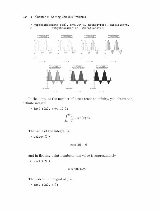
234 • Chapter 7: Solving Calculus Problems
> ApproximateInt( f(x), x=0..4*Pi, method=left, partition=6,> output=animation, iterations=7);
f(x)
An Approximation of the Integral off(x) = 1/2+sin(x)
on the Interval [0, 4*Pi]Using a Left-endpoint Riemann Sum
Approximate Value: 6.283185307
Area: 6.283185309–1
–0.5
0
0.5
1
1.5
2 4 6 8 10 12x
f(x)
An Approximation of the Integral off(x) = 1/2+sin(x)
on the Interval [0, 4*Pi]Using a Left-endpoint Riemann Sum
Approximate Value: 6.283185307
Area: 6.283185308–1
–0.5
0
0.5
1
1.5
2 4 6 8 10 12x
f(x)
An Approximation of the Integral off(x) = 1/2+sin(x)
on the Interval [0, 4*Pi]Using a Left-endpoint Riemann Sum
Approximate Value: 6.283185307
Area: 6.283185308–1
–0.5
0
0.5
1
1.5
2 4 6 8 10 12x
f(x)
An Approximation of the Integral off(x) = 1/2+sin(x)
on the Interval [0, 4*Pi]Using a Left-endpoint Riemann Sum
Approximate Value: 6.283185307
Area: 6.283185311–1
–0.5
0
0.5
1
1.5
2 4 6 8 10 12x
f(x)
An Approximation of the Integral off(x) = 1/2+sin(x)
on the Interval [0, 4*Pi]Using a Left-endpoint Riemann Sum
Approximate Value: 6.283185307
Area: 6.283185308–1
–0.5
0
0.5
1
1.5
2 4 6 8 10 12x
f(x)
An Approximation of the Integral off(x) = 1/2+sin(x)
on the Interval [0, 4*Pi]Using a Left-endpoint Riemann Sum
Approximate Value: 6.283185307
Area: 6.283185309–1
–0.5
0
0.5
1
1.5
2 4 6 8 10 12x
f(x)
An Approximation of the Integral off(x) = 1/2+sin(x)
on the Interval [0, 4*Pi]Using a Left-endpoint Riemann Sum
Approximate Value: 6.283185307
Area: 6.283185309–1
–0.5
0
0.5
1
1.5
2 4 6 8 10 12x
In the limit, as the number of boxes tends to infinity, you obtain thedefinite integral.
> Int( f(x), x=0..10 );
∫ 10
0
1
2+ sin(x) dx
The value of the integral is
> value( % );
−cos(10) + 6
and in floating-point numbers, this value is approximately
> evalf( % );
6.839071529
The indefinite integral of f is
> Int( f(x), x );
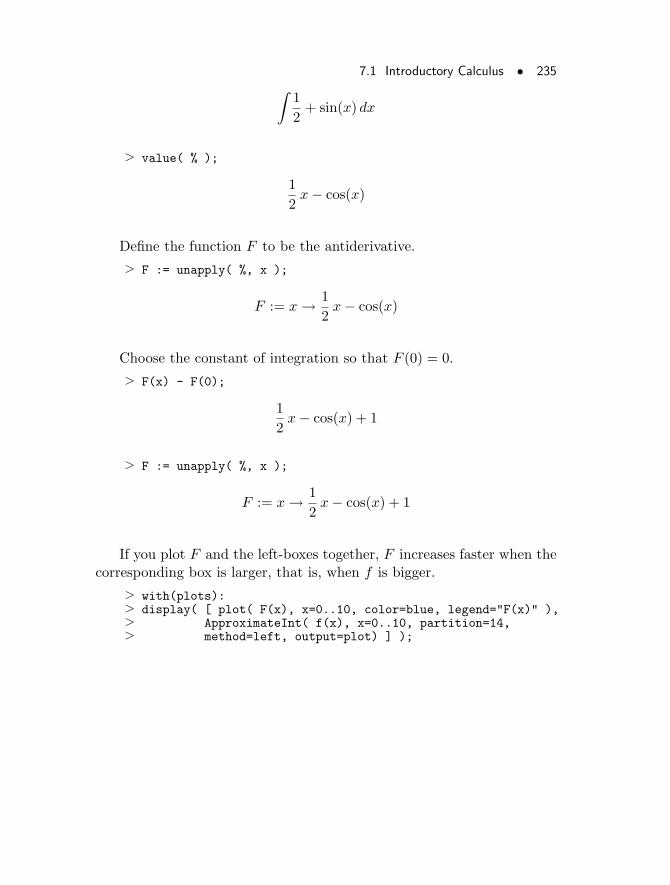
7.1 Introductory Calculus • 235
∫
1
2+ sin(x) dx
> value( % );
1
2x− cos(x)
Define the function F to be the antiderivative.
> F := unapply( %, x );
F := x → 1
2x− cos(x)
Choose the constant of integration so that F (0) = 0.
> F(x) - F(0);
1
2x− cos(x) + 1
> F := unapply( %, x );
F := x → 1
2x− cos(x) + 1
If you plot F and the left-boxes together, F increases faster when thecorresponding box is larger, that is, when f is bigger.
> with(plots):> display( [ plot( F(x), x=0..10, color=blue, legend="F(x)" ),> ApproximateInt( f(x), x=0..10, partition=14,> method=left, output=plot) ] );
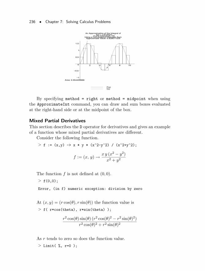
236 • Chapter 7: Solving Calculus Problems
F(x)f(x)
An Approximation of the Integral off(x) = 1/2+sin(x)
on the Interval [0, 10]Using a Left-endpoint Riemann Sum
Approximate Value: 6.839071529
Area: 6.954499888–1
–0.5
0
0.5
1
1.5
2 4 6 8 10x
By specifying method = right or method = midpoint when usingthe ApproximateInt command, you can draw and sum boxes evaluatedat the right-hand side or at the midpoint of the box.
Mixed Partial DerivativesThis section describes the D operator for derivatives and gives an exampleof a function whose mixed partial derivatives are different.
Consider the following function.
> f := (x,y) -> x * y * (x^2-y^2) / (x^2+y^2);
f := (x, y) → x y (x2 − y2)
x2 + y2
The function f is not defined at (0, 0).
> f(0,0);
Error, (in f) numeric exception: division by zero
At (x, y) = (r cos(θ), r sin(θ)) the function value is
> f( r*cos(theta), r*sin(theta) );
r2 cos(θ) sin(θ) (r2 cos(θ)2 − r2 sin(θ)2)
r2 cos(θ)2 + r2 sin(θ)2
As r tends to zero so does the function value.
> Limit( %, r=0 );
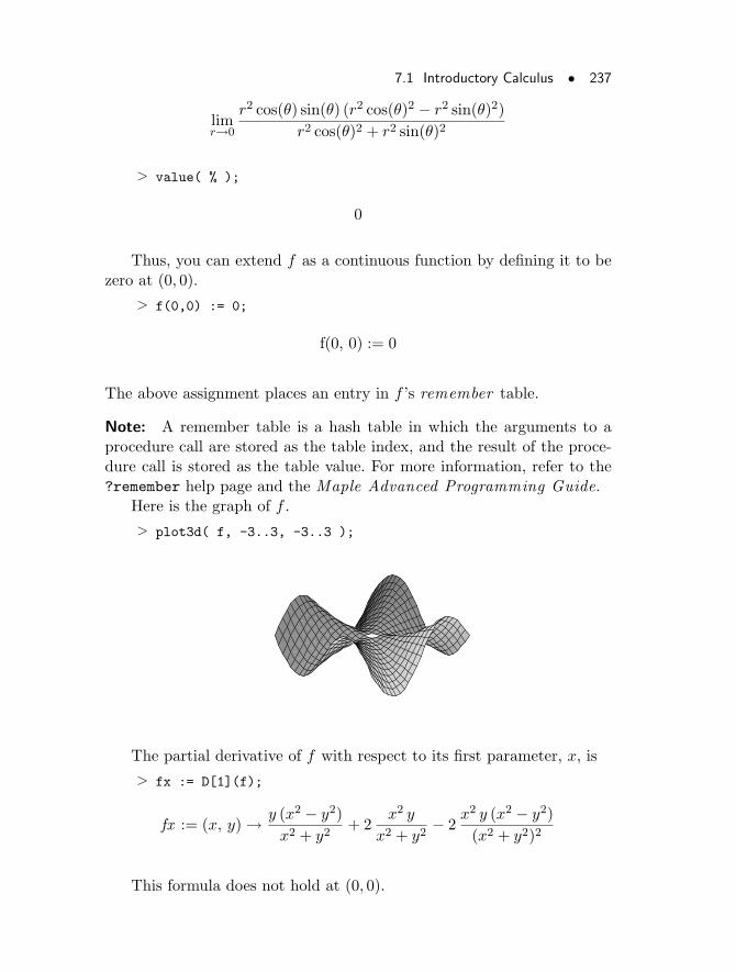
7.1 Introductory Calculus • 237
limr→0
r2 cos(θ) sin(θ) (r2 cos(θ)2 − r2 sin(θ)2)
r2 cos(θ)2 + r2 sin(θ)2
> value( % );
0
Thus, you can extend f as a continuous function by defining it to bezero at (0, 0).
> f(0,0) := 0;
f(0, 0) := 0
The above assignment places an entry in f ’s remember table.
Note: A remember table is a hash table in which the arguments to aprocedure call are stored as the table index, and the result of the proce-dure call is stored as the table value. For more information, refer to the?remember help page and the Maple Advanced Programming Guide.
Here is the graph of f .
> plot3d( f, -3..3, -3..3 );
The partial derivative of f with respect to its first parameter, x, is
> fx := D[1](f);
fx := (x, y) → y (x2 − y2)
x2 + y2+ 2
x2 y
x2 + y2− 2
x2 y (x2 − y2)
(x2 + y2)2
This formula does not hold at (0, 0).
238 • Chapter 7: Solving Calculus Problems
> fx(0,0);
Error, (in fx) numeric exception: division by zero
Therefore, you must use the limit definition of the derivative.
> fx(0,0) := limit( ( f(h,0) - f(0,0) )/h, h=0 );
fx(0, 0) := 0
At (x, y) = (r cos(θ), r sin(θ)) the value of fx is
> fx( r*cos(theta), r*sin(theta) );
r sin(θ) (r2 cos(θ)2 − r2 sin(θ)2)
r2 cos(θ)2 + r2 sin(θ)2+ 2
r3 cos(θ)2 sin(θ)
r2 cos(θ)2 + r2 sin(θ)2
− 2r3 cos(θ)2 sin(θ) (r2 cos(θ)2 − r2 sin(θ)2)
(r2 cos(θ)2 + r2 sin(θ)2)2
> combine( % );
3
4r sin(3 θ)− 1
4r sin(5 θ)
As the distance r from (x, y) to (0, 0) tends to zero, so does |fx(x, y)−fx(0, 0)|.
> Limit( abs( % - fx(0,0) ), r=0 );
limr→0
∣
∣
∣
∣
−3
4r sin(3 θ) +
1
4r sin(5 θ)
∣
∣
∣
∣
> value( % );
0
Hence, fx is continuous at (0, 0).By symmetry, the same arguments apply to the derivative of f with
respect to its second parameter, y.
> fy := D[2](f);
7.1 Introductory Calculus • 239
fy := (x, y) → x (x2 − y2)
x2 + y2− 2
x y2
x2 + y2− 2
x y2 (x2 − y2)
(x2 + y2)2
> fy(0,0) := limit( ( f(0,k) - f(0,0) )/k, k=0 );
fy(0, 0) := 0
Here is a mixed second derivative of f .
> fxy := D[1,2](f);
fxy := (x, y) → x2 − y2
x2 + y2+ 2
x2
x2 + y2− 2
x2 (x2 − y2)
(x2 + y2)2
− 2y2
x2 + y2− 2
y2 (x2 − y2)
(x2 + y2)2+ 8
x2 y2 (x2 − y2)
(x2 + y2)3
Again, the formula does not hold at (0, 0).
> fxy(0,0);
Error, (in fxy) numeric exception: division by zero
The limit definition is
> Limit( ( fx(0,k) - fx(0,0) )/k, k=0 );
limk→0
− 1
> fxy(0,0) := value( % );
fxy(0, 0) := −1
The other mixed second derivative is
> fyx := D[2,1](f);
fyx := (x, y) → x2 − y2
x2 + y2+ 2
x2
x2 + y2− 2
x2 (x2 − y2)
(x2 + y2)2
− 2y2
x2 + y2− 2
y2 (x2 − y2)
(x2 + y2)2+ 8
x2 y2 (x2 − y2)
(x2 + y2)3
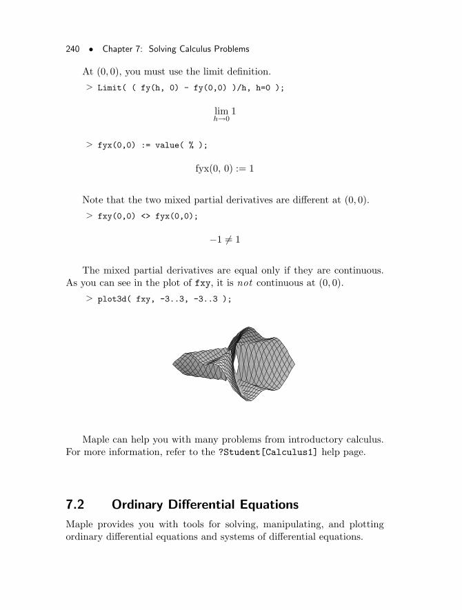
240 • Chapter 7: Solving Calculus Problems
At (0, 0), you must use the limit definition.
> Limit( ( fy(h, 0) - fy(0,0) )/h, h=0 );
limh→0
1
> fyx(0,0) := value( % );
fyx(0, 0) := 1
Note that the two mixed partial derivatives are different at (0, 0).
> fxy(0,0) <> fyx(0,0);
−1 6= 1
The mixed partial derivatives are equal only if they are continuous.As you can see in the plot of fxy, it is not continuous at (0, 0).
> plot3d( fxy, -3..3, -3..3 );
Maple can help you with many problems from introductory calculus.For more information, refer to the ?Student[Calculus1] help page.
7.2 Ordinary Differential Equations
Maple provides you with tools for solving, manipulating, and plottingordinary differential equations and systems of differential equations.
7.2 Ordinary Differential Equations • 241
The dsolve CommandThe most commonly used command for investigating the behavior of or-dinary differential equations (ODEs) in Maple is dsolve. You can usethis general-purpose command to obtain both closed form and numericalsolutions to a wide variety of ODEs. This is the basic syntax of dsolve.
dsolve(eqns, vars)
• eqns is a set of differential equations and initial values
• vars is a set of variables with respect to which dsolve solves
The following example is a differential equation and an initial condi-tion.
> eq := diff(v(t),t)+2*t = 0;
eq := (d
dtv(t)) + 2 t = 0
> ini := v(1) = 5;
ini := v(1) = 5
Use dsolve to obtain the solution.
> dsolve( {eq, ini}, {v(t)} );
v(t) = −t2 + 6
If you omit some or all of the initial conditions, then dsolve returnsa solution containing arbitrary constants of the form _Cnumber .
> eq := diff(y(x),x$2) - y(x) = 1;
eq := (d2
dx2y(x))− y(x) = 1
> dsolve( {eq}, {y(x)} );
{y(x) = ex_C2 + e(−x)_C1 − 1}
242 • Chapter 7: Solving Calculus Problems
To specify initial conditions for the derivative of a function, use thefollowing notation.
D(fcn)(var_value) = value
(D@@n)(fcn)(var_value) = value
• D notation represents the derivative
• D@@n notation represents the nth derivative
Here is a differential equation and some initial conditions involving thederivative.
> de1 := diff(y(t),t$2) + 5*diff(y(t),t) + 6*y(t) = 0;
de1 := (d2
dt2y(t)) + 5 (
d
dty(t)) + 6 y(t) = 0
> ini := y(0)=0, D(y)(0)=1;
ini := y(0) = 0, D(y)(0) = 1
Again, use dsolve to find the solution.
> dsolve( {de1, ini}, {y(t)} );
y(t) = −e(−3 t) + e(−2 t)
Additionally, dsolve may return a solution in parametric form,[x=f(_T), y(x)=g(_T)], where _T is the parameter.
The explicit Option Maple may return the solution to a differentialequation in implicit form.
> de2 := diff(y(x),x$2) = (ln(y(x))+1)*diff(y(x),x);
de2 :=d2
dx2y(x) = (ln(y(x)) + 1) (
d
dxy(x))
> dsolve( {de2}, {y(x)} );
7.2 Ordinary Differential Equations • 243
{y(x) = _C1 },
{
∫ y(x) 1
_a ln(_a) + _C1d_a − x−_C2 = 0
}
Use the explicit option to search for an explicit solution for the firstresult.
> dsolve( {de2}, {y(x)}, explicit );
{y(x) = _C1 },{
y(x) = RootOf
(
−∫ _Z 1
_f ln(_f ) + _C1d_f + x+_C2
)}
However, in some cases, Maple may not be able to find an explicitsolution. There is also an implicit option to force answers to be returnedin implicit form.
The method=laplace Option Applying Laplace transform methods todifferential equations often reduces the complexity of the problem. Thetransform maps the differential equations into algebraic equations, whichare much easier to solve. The difficulty is in the transformation of theequations to the new domain, and especially the transformation of thesolutions back.
The Laplace transform method can handle linear ODEs of arbitraryorder, and some cases of linear ODEs with non-constant coefficients, pro-vided that Maple can find the transforms. This method can also solvesystems of coupled equations.
Consider the following problem in classical dynamics. Two weightswith masses m and αm, respectively, rest on a frictionless plane joined bya spring with spring constant k. What are the trajectories of each weightif the first weight is subject to a unit step force u(t) at time t = 1? First,set up the differential equations that govern the system. Newton’s SecondLaw governs the motion of the first weight, and hence, the mass m timesthe acceleration must equal the sum of the forces that you apply to thefirst weight, including the external force u(t).
> eqn1 :=> alpha*m*diff(x[1](t),t$2) = k*(x[2](t) - x[1](t)) + u(t);
eqn1 := αm (d2
dt2x1(t)) = k (x2(t)− x1(t)) + u(t)
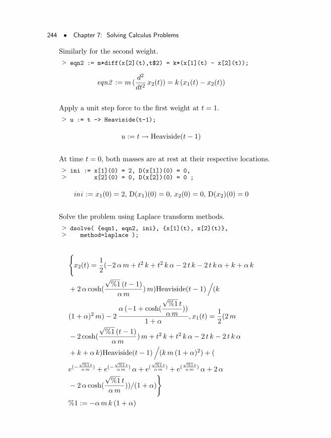
244 • Chapter 7: Solving Calculus Problems
Similarly for the second weight.
> eqn2 := m*diff(x[2](t),t$2) = k*(x[1](t) - x[2](t));
eqn2 := m (d2
dt2x2(t)) = k (x1(t)− x2(t))
Apply a unit step force to the first weight at t = 1.
> u := t -> Heaviside(t-1);
u := t → Heaviside(t− 1)
At time t = 0, both masses are at rest at their respective locations.
> ini := x[1](0) = 2, D(x[1])(0) = 0,> x[2](0) = 0, D(x[2])(0) = 0 ;
ini := x1(0) = 2, D(x1)(0) = 0, x2(0) = 0, D(x2)(0) = 0
Solve the problem using Laplace transform methods.
> dsolve( {eqn1, eqn2, ini}, {x[1](t), x[2](t)},> method=laplace );
{
x2(t) =1
2(−2αm+ t2 k + t2 k α− 2 t k − 2 t k α+ k + αk
+ 2α cosh(
√%1 (t− 1)
αm)m)Heaviside(t− 1)
/
(k
(1 + α)2m)− 2α (−1 + cosh(
√%1 t
αm))
1 + α, x1(t) =
1
2(2m
− 2 cosh(
√%1 (t− 1)
αm)m+ t2 k + t2 k α− 2 t k − 2 t k α
+ k + αk)Heaviside(t− 1)/
(km (1 + α)2) + (
e(−√%1 tαm
) + e(−√%1 tαm
) α+ e(√%1 tαm
) + e(√%1 tαm
) α+ 2α
− 2α cosh(
√%1 t
αm))/(1 + α)
}
%1 := −αmk (1 + α)
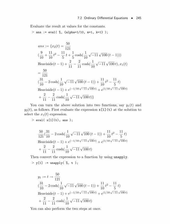
7.2 Ordinary Differential Equations • 245
Evaluate the result at values for the constants.
> ans := eval( %, {alpha=1/10, m=1, k=1} );
ans := {x2(t) =50
121
(9
10+
11
10t2 − 11
5t+
1
5cosh(
1
10
√−11
√100 (t− 1)))
Heaviside(t− 1) +2
11− 2
11cosh(
1
10
√−11
√100 t), x1(t)
=50
121
(31
10− 2 cosh(
1
10
√−11
√100 (t− 1)) +
11
10t2 − 11
5t)
Heaviside(t− 1) + e(−1/10√−11
√100 t) + e(1/10
√−11
√100 t)
+2
11− 2
11cosh(
1
10
√−11
√100 t)}
You can turn the above solution into two functions, say y1(t) andy2(t), as follows. First evaluate the expression x[1](t) at the solution toselect the x1(t) expression.
> eval( x[1](t), ans );
50
121(31
10− 2 cosh(
1
10
√−11
√100 (t− 1)) +
11
10t2 − 11
5t)
Heaviside(t− 1) + e(−1/10√−11
√100 t) + e(1/10
√−11
√100 t)
+2
11− 2
11cosh(
1
10
√−11
√100 t)
Then convert the expression to a function by using unapply.
> y[1] := unapply( %, t );
y1 := t → 50
121
(31
10− 2 cosh(
1
10
√−11
√100 (t− 1)) +
11
10t2 − 11
5t)
Heaviside(t− 1) + e(−1/10√−11
√100 t) + e(1/10
√−11
√100 t)
+2
11− 2
11cosh(
1
10
√−11
√100 t)
You can also perform the two steps at once.
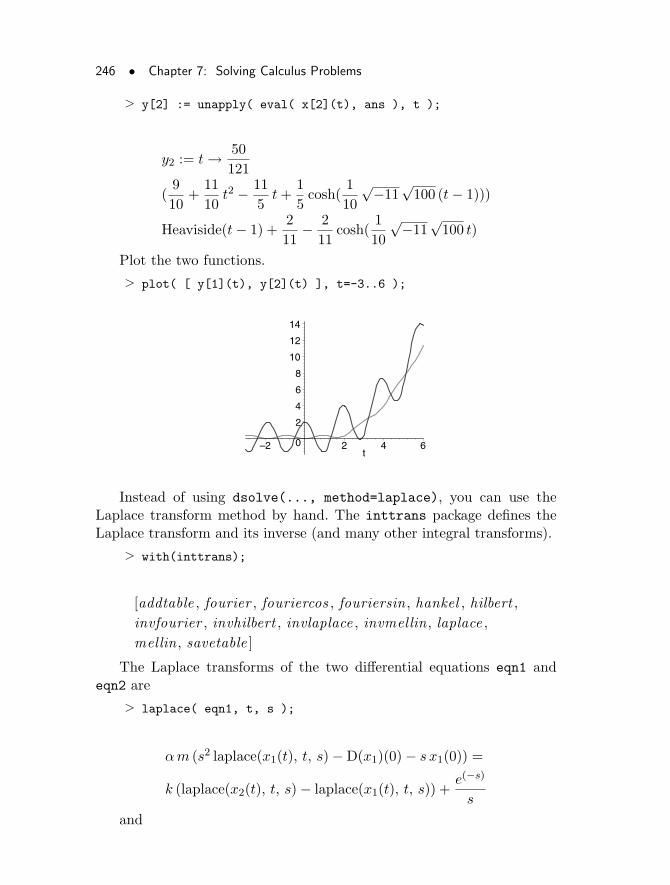
246 • Chapter 7: Solving Calculus Problems
> y[2] := unapply( eval( x[2](t), ans ), t );
y2 := t → 50
121
(9
10+
11
10t2 − 11
5t+
1
5cosh(
1
10
√−11
√100 (t− 1)))
Heaviside(t− 1) +2
11− 2
11cosh(
1
10
√−11
√100 t)
Plot the two functions.
> plot( [ y[1](t), y[2](t) ], t=-3..6 );
0
2
4
6
8
10
12
14
–2 2 4 6t
Instead of using dsolve(..., method=laplace), you can use theLaplace transform method by hand. The inttrans package defines theLaplace transform and its inverse (and many other integral transforms).
> with(inttrans);
[addtable , fourier , fouriercos , fouriersin, hankel , hilbert ,
invfourier , invhilbert , invlaplace , invmellin, laplace ,
mellin, savetable ]
The Laplace transforms of the two differential equations eqn1 andeqn2 are
> laplace( eqn1, t, s );
αm (s2 laplace(x1(t), t, s)−D(x1)(0)− s x1(0)) =
k (laplace(x2(t), t, s)− laplace(x1(t), t, s)) +e(−s)
s
and
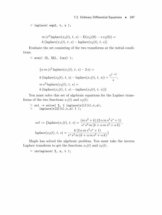
7.2 Ordinary Differential Equations • 247
> laplace( eqn2, t, s );
m (s2 laplace(x2(t), t, s)−D(x2)(0)− s x2(0)) =
k (laplace(x1(t), t, s)− laplace(x2(t), t, s))
Evaluate the set consisting of the two transforms at the initial condi-tions.
> eval( {%, %%}, {ini} );
{αm (s2 laplace(x1(t), t, s)− 2 s) =
k (laplace(x2(t), t, s)− laplace(x1(t), t, s)) +e(−s)
s,
m s2 laplace(x2(t), t, s) =
k (laplace(x1(t), t, s)− laplace(x2(t), t, s))}You must solve this set of algebraic equations for the Laplace trans-
forms of the two functions x1(t) and x2(t).
> sol := solve( %, { laplace(x[1](t),t,s),> laplace(x[2](t),t,s) } );
sol := {laplace(x1(t), t, s) =(ms2 + k) (2αms2 es + 1)
es s3m (k + αms2 + αk),
laplace(x2(t), t, s) =k (2αms2 es + 1)
es s3m (k + αms2 + αk)}
Maple has solved the algebraic problem. You must take the inverseLaplace transform to get the functions x1(t) and x2(t) .
> invlaplace( %, s, t );
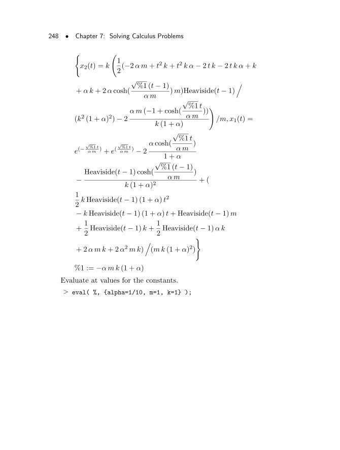
248 • Chapter 7: Solving Calculus Problems
{
x2(t) = k
(
1
2(−2αm+ t2 k + t2 k α− 2 t k − 2 t k α+ k
+ αk + 2α cosh(
√%1 (t− 1)
αm)m)Heaviside(t− 1)
/
(k2 (1 + α)2)− 2αm (−1 + cosh(
√%1 t
αm))
k (1 + α)
)
/m, x1(t) =
e(−√
%1 tαm
) + e(√%1 tαm
) − 2α cosh(
√%1 t
αm)
1 + α
−Heaviside(t− 1) cosh(
√%1 (t− 1)
αm)
k (1 + α)2+ (
1
2kHeaviside(t− 1) (1 + α) t2
− kHeaviside(t− 1) (1 + α) t+Heaviside(t− 1)m
+1
2Heaviside(t− 1) k +
1
2Heaviside(t− 1)αk
+ 2αmk + 2α2mk)/
(mk (1 + α)2)
}
%1 := −αmk (1 + α)
Evaluate at values for the constants.
> eval( %, {alpha=1/10, m=1, k=1} );
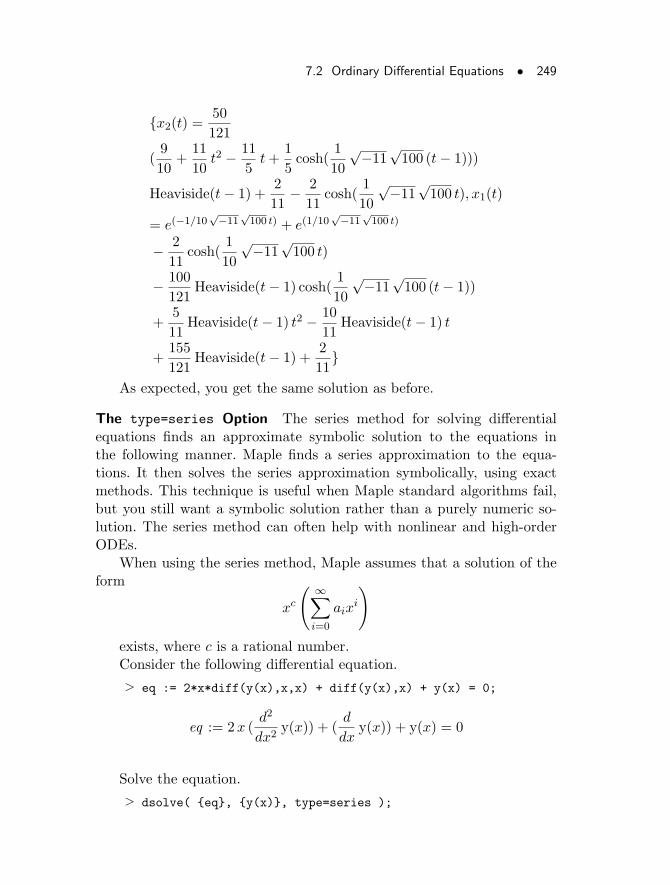
7.2 Ordinary Differential Equations • 249
{x2(t) =50
121
(9
10+
11
10t2 − 11
5t+
1
5cosh(
1
10
√−11
√100 (t− 1)))
Heaviside(t− 1) +2
11− 2
11cosh(
1
10
√−11
√100 t), x1(t)
= e(−1/10√−11
√100 t) + e(1/10
√−11
√100 t)
− 2
11cosh(
1
10
√−11
√100 t)
− 100
121Heaviside(t− 1) cosh(
1
10
√−11
√100 (t− 1))
+5
11Heaviside(t− 1) t2 − 10
11Heaviside(t− 1) t
+155
121Heaviside(t− 1) +
2
11}
As expected, you get the same solution as before.
The type=series Option The series method for solving differentialequations finds an approximate symbolic solution to the equations inthe following manner. Maple finds a series approximation to the equa-tions. It then solves the series approximation symbolically, using exactmethods. This technique is useful when Maple standard algorithms fail,but you still want a symbolic solution rather than a purely numeric so-lution. The series method can often help with nonlinear and high-orderODEs.
When using the series method, Maple assumes that a solution of theform
xc
( ∞∑
i=0
aixi
)
exists, where c is a rational number.Consider the following differential equation.
> eq := 2*x*diff(y(x),x,x) + diff(y(x),x) + y(x) = 0;
eq := 2x (d2
dx2y(x)) + (
d
dxy(x)) + y(x) = 0
Solve the equation.
> dsolve( {eq}, {y(x)}, type=series );
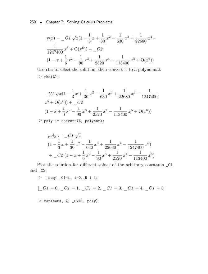
250 • Chapter 7: Solving Calculus Problems
y(x) = _C1√x(1− 1
3x+
1
30x2 − 1
630x3 +
1
22680x4−
1
1247400x5 +O(x6)) + _C2
(1− x+1
6x2 − 1
90x3 +
1
2520x4 − 1
113400x5 +O(x6))
Use rhs to select the solution, then convert it to a polynomial.
> rhs(%);
_C1√x(1− 1
3x+
1
30x2 − 1
630x3 +
1
22680x4 − 1
1247400
x5 +O(x6)) + _C2
(1− x+1
6x2 − 1
90x3 +
1
2520x4 − 1
113400x5 +O(x6))
> poly := convert(%, polynom);
poly := _C1√x
(1− 1
3x+
1
30x2 − 1
630x3 +
1
22680x4 − 1
1247400x5)
+ _C2 (1− x+1
6x2 − 1
90x3 +
1
2520x4 − 1
113400x5)
Plot the solution for different values of the arbitrary constants _C1
and _C2.
> [ seq( _C1=i, i=0..5 ) ];
[_C1 = 0, _C1 = 1, _C1 = 2, _C1 = 3, _C1 = 4, _C1 = 5]
> map(subs, %, _C2=1, poly);
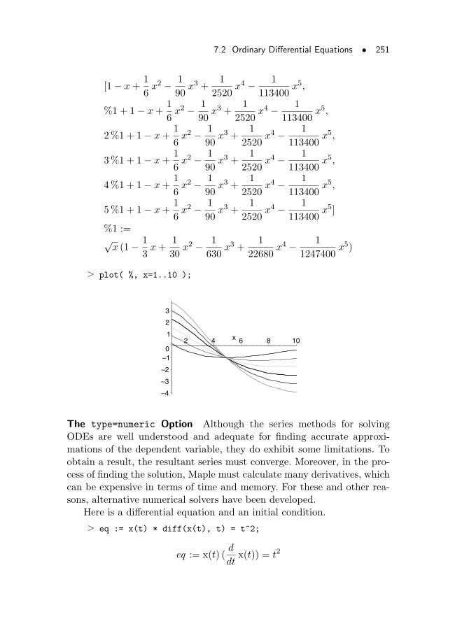
7.2 Ordinary Differential Equations • 251
[1− x+1
6x2 − 1
90x3 +
1
2520x4 − 1
113400x5,
%1 + 1− x+1
6x2 − 1
90x3 +
1
2520x4 − 1
113400x5,
2%1 + 1− x+1
6x2 − 1
90x3 +
1
2520x4 − 1
113400x5,
3%1 + 1− x+1
6x2 − 1
90x3 +
1
2520x4 − 1
113400x5,
4%1 + 1− x+1
6x2 − 1
90x3 +
1
2520x4 − 1
113400x5,
5%1 + 1− x+1
6x2 − 1
90x3 +
1
2520x4 − 1
113400x5]
%1 :=√x (1− 1
3x+
1
30x2 − 1
630x3 +
1
22680x4 − 1
1247400x5)
> plot( %, x=1..10 );
–4
–3
–2
–10
1
2
3
2 4 6 8 10x
The type=numeric Option Although the series methods for solvingODEs are well understood and adequate for finding accurate approxi-mations of the dependent variable, they do exhibit some limitations. Toobtain a result, the resultant series must converge. Moreover, in the pro-cess of finding the solution, Maple must calculate many derivatives, whichcan be expensive in terms of time and memory. For these and other rea-sons, alternative numerical solvers have been developed.
Here is a differential equation and an initial condition.
> eq := x(t) * diff(x(t), t) = t^2;
eq := x(t) (d
dtx(t)) = t2
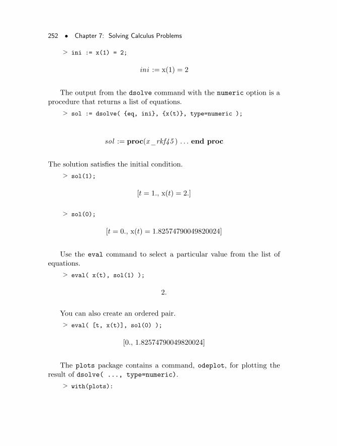
252 • Chapter 7: Solving Calculus Problems
> ini := x(1) = 2;
ini := x(1) = 2
The output from the dsolve command with the numeric option is aprocedure that returns a list of equations.
> sol := dsolve( {eq, ini}, {x(t)}, type=numeric );
sol := proc(x_rkf45 ) . . . end proc
The solution satisfies the initial condition.
> sol(1);
[t = 1., x(t) = 2.]
> sol(0);
[t = 0., x(t) = 1.82574790049820024]
Use the eval command to select a particular value from the list ofequations.
> eval( x(t), sol(1) );
2.
You can also create an ordered pair.
> eval( [t, x(t)], sol(0) );
[0., 1.82574790049820024]
The plots package contains a command, odeplot, for plotting theresult of dsolve( ..., type=numeric).
> with(plots):
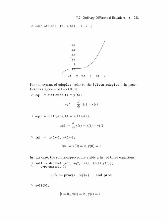
7.2 Ordinary Differential Equations • 253
> odeplot( sol, [t, x(t)], -1..2 );
1.8
2
2.2
2.4
2.6
2.8
x
–1 –0.5 0 0.5 1 1.5 2t
For the syntax of odeplot, refer to the ?plots,odeplot help page.Here is a system of two ODEs.
> eq1 := diff(x(t),t) = y(t);
eq1 :=d
dtx(t) = y(t)
> eq2 := diff(y(t),t) = x(t)+y(t);
eq2 :=d
dty(t) = x(t) + y(t)
> ini := x(0)=2, y(0)=1;
ini := x(0) = 2, y(0) = 1
In this case, the solution-procedure yields a list of three equations.
> sol1 := dsolve( {eq1, eq2, ini}, {x(t),y(t)},> type=numeric );
sol1 := proc(x_rkf45 ) . . . end proc
> sol1(0);
[t = 0., x(t) = 2., y(t) = 1.]
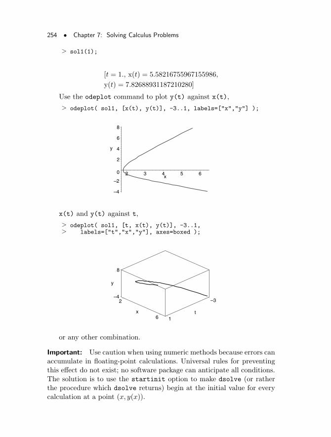
254 • Chapter 7: Solving Calculus Problems
> sol1(1);
[t = 1., x(t) = 5.58216755967155986,
y(t) = 7.82688931187210280]
Use the odeplot command to plot y(t) against x(t),
> odeplot( sol1, [x(t), y(t)], -3..1, labels=["x","y"] );
–4
–2
0
2
4
6
8
y
2 3 4 5 6x
x(t) and y(t) against t,
> odeplot( sol1, [t, x(t), y(t)], -3..1,> labels=["t","x","y"], axes=boxed );
–3
1t
2
6x
–4
8
y
or any other combination.
Important: Use caution when using numeric methods because errors canaccumulate in floating-point calculations. Universal rules for preventingthis effect do not exist; no software package can anticipate all conditions.The solution is to use the startinit option to make dsolve (or ratherthe procedure which dsolve returns) begin at the initial value for everycalculation at a point (x, y(x)).
7.2 Ordinary Differential Equations • 255
You can specify which algorithm dsolve(..., type=numeric) useswhen solving your differential equation. Refer to the ?dsolve,numeric
help page.
Example: Taylor SeriesIn its general form, a series method solution to an ODE requires theforming of a Taylor series about t = 0 for some function f(t). Thus, youmust be able to obtain and manipulate the higher order derivatives ofyour function, f ′(t), f ′′(t), f ′′′(t), and so on.
Once you have obtained the derivatives, substitute them into the Tay-lor series representation of f(t).
> taylor(f(t), t);
f(0) + D(f)(0) t+1
2(D(2))(f)(0) t2 +
1
6(D(3))(f)(0) t3+
1
24(D(4))(f)(0) t4 +
1
120(D(5))(f)(0) t5 +O(t6)
As an example, consider Newton’s Law of Cooling:
dθ
dt= − 1
10(θ − 20), θ(0) = 100.
Using the D operator, enter the above equation into Maple.
> eq := D(theta) = -1/10*(theta-20);
eq := D(θ) = − 1
10θ + 2
> ini := theta(0)=100;
ini := θ(0) = 100
First obtain the required number of higher derivatives. Determine thisnumber from the order of your Taylor series. If you use the default valueof Order that Maple provides,
> Order;
6
then you must generate derivatives up to order
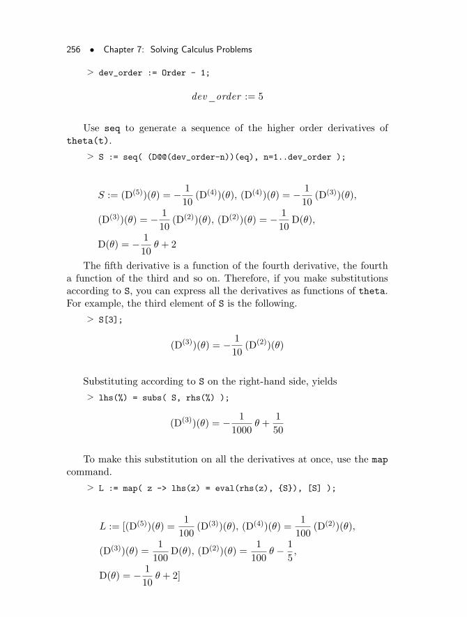
256 • Chapter 7: Solving Calculus Problems
> dev_order := Order - 1;
dev_order := 5
Use seq to generate a sequence of the higher order derivatives oftheta(t).
> S := seq( (D@@(dev_order-n))(eq), n=1..dev_order );
S := (D(5))(θ) = − 1
10(D(4))(θ), (D(4))(θ) = − 1
10(D(3))(θ),
(D(3))(θ) = − 1
10(D(2))(θ), (D(2))(θ) = − 1
10D(θ),
D(θ) = − 1
10θ + 2
The fifth derivative is a function of the fourth derivative, the fourtha function of the third and so on. Therefore, if you make substitutionsaccording to S, you can express all the derivatives as functions of theta.For example, the third element of S is the following.
> S[3];
(D(3))(θ) = − 1
10(D(2))(θ)
Substituting according to S on the right-hand side, yields
> lhs(%) = subs( S, rhs(%) );
(D(3))(θ) = − 1
1000θ +
1
50
To make this substitution on all the derivatives at once, use the map
command.
> L := map( z -> lhs(z) = eval(rhs(z), {S}), [S] );
L := [(D(5))(θ) =1
100(D(3))(θ), (D(4))(θ) =
1
100(D(2))(θ),
(D(3))(θ) =1
100D(θ), (D(2))(θ) =
1
100θ − 1
5,
D(θ) = − 1
10θ + 2]
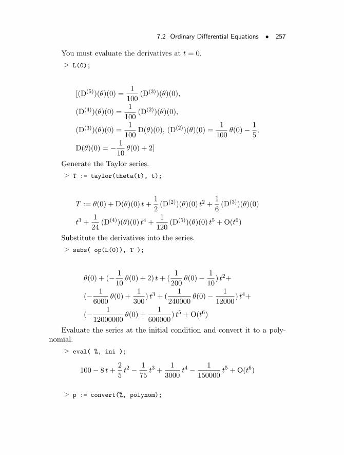
7.2 Ordinary Differential Equations • 257
You must evaluate the derivatives at t = 0.
> L(0);
[(D(5))(θ)(0) =1
100(D(3))(θ)(0),
(D(4))(θ)(0) =1
100(D(2))(θ)(0),
(D(3))(θ)(0) =1
100D(θ)(0), (D(2))(θ)(0) =
1
100θ(0)− 1
5,
D(θ)(0) = − 1
10θ(0) + 2]
Generate the Taylor series.
> T := taylor(theta(t), t);
T := θ(0) + D(θ)(0) t+1
2(D(2))(θ)(0) t2 +
1
6(D(3))(θ)(0)
t3 +1
24(D(4))(θ)(0) t4 +
1
120(D(5))(θ)(0) t5 +O(t6)
Substitute the derivatives into the series.
> subs( op(L(0)), T );
θ(0) + (− 1
10θ(0) + 2) t+ (
1
200θ(0)− 1
10) t2+
(− 1
6000θ(0) +
1
300) t3 + (
1
240000θ(0)− 1
12000) t4+
(− 1
12000000θ(0) +
1
600000) t5 +O(t6)
Evaluate the series at the initial condition and convert it to a poly-nomial.
> eval( %, ini );
100− 8 t+2
5t2 − 1
75t3 +
1
3000t4 − 1
150000t5 +O(t6)
> p := convert(%, polynom);
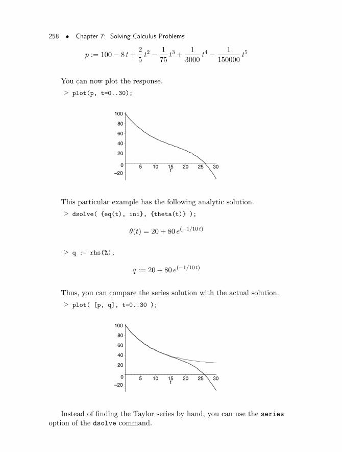
258 • Chapter 7: Solving Calculus Problems
p := 100− 8 t+2
5t2 − 1
75t3 +
1
3000t4 − 1
150000t5
You can now plot the response.
> plot(p, t=0..30);
–20
0
20
40
60
80
100
5 10 15 20 25 30t
This particular example has the following analytic solution.
> dsolve( {eq(t), ini}, {theta(t)} );
θ(t) = 20 + 80 e(−1/10 t)
> q := rhs(%);
q := 20 + 80 e(−1/10 t)
Thus, you can compare the series solution with the actual solution.
> plot( [p, q], t=0..30 );
–20
0
20
40
60
80
100
5 10 15 20 25 30t
Instead of finding the Taylor series by hand, you can use the series
option of the dsolve command.
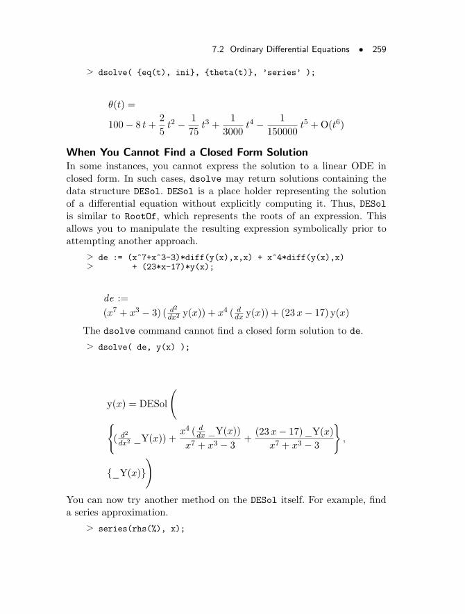
7.2 Ordinary Differential Equations • 259
> dsolve( {eq(t), ini}, {theta(t)}, ’series’ );
θ(t) =
100− 8 t+2
5t2 − 1
75t3 +
1
3000t4 − 1
150000t5 +O(t6)
When You Cannot Find a Closed Form SolutionIn some instances, you cannot express the solution to a linear ODE inclosed form. In such cases, dsolve may return solutions containing thedata structure DESol. DESol is a place holder representing the solutionof a differential equation without explicitly computing it. Thus, DESolis similar to RootOf, which represents the roots of an expression. Thisallows you to manipulate the resulting expression symbolically prior toattempting another approach.
> de := (x^7+x^3-3)*diff(y(x),x,x) + x^4*diff(y(x),x)> + (23*x-17)*y(x);
de :=
(x7 + x3 − 3) ( d2
dx2 y(x)) + x4 ( ddx y(x)) + (23x− 17) y(x)
The dsolve command cannot find a closed form solution to de.
> dsolve( de, y(x) );
y(x) = DESol
(
{
( d2
dx2 _Y(x)) +x4 ( d
dx _Y(x))
x7 + x3 − 3+
(23x− 17)_Y(x)
x7 + x3 − 3
}
,
{_Y(x)}
)
You can now try another method on the DESol itself. For example, finda series approximation.
> series(rhs(%), x);
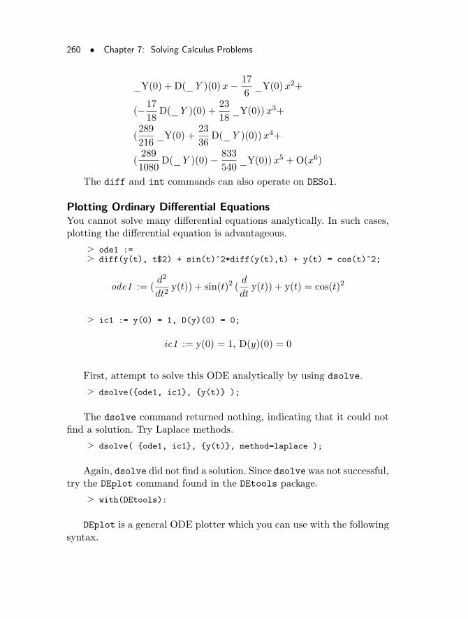
260 • Chapter 7: Solving Calculus Problems
_Y(0) + D(_Y )(0)x− 17
6_Y(0)x2+
(−17
18D(_Y )(0) +
23
18_Y(0))x3+
(289
216_Y(0) +
23
36D(_Y )(0))x4+
(289
1080D(_Y )(0)− 833
540_Y(0))x5 +O(x6)
The diff and int commands can also operate on DESol.
Plotting Ordinary Differential EquationsYou cannot solve many differential equations analytically. In such cases,plotting the differential equation is advantageous.
> ode1 :=> diff(y(t), t$2) + sin(t)^2*diff(y(t),t) + y(t) = cos(t)^2;
ode1 := (d2
dt2y(t)) + sin(t)2 (
d
dty(t)) + y(t) = cos(t)2
> ic1 := y(0) = 1, D(y)(0) = 0;
ic1 := y(0) = 1, D(y)(0) = 0
First, attempt to solve this ODE analytically by using dsolve.
> dsolve({ode1, ic1}, {y(t)} );
The dsolve command returned nothing, indicating that it could notfind a solution. Try Laplace methods.
> dsolve( {ode1, ic1}, {y(t)}, method=laplace );
Again, dsolve did not find a solution. Since dsolve was not successful,try the DEplot command found in the DEtools package.
> with(DEtools):
DEplot is a general ODE plotter which you can use with the followingsyntax.
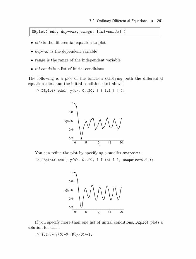
7.2 Ordinary Differential Equations • 261
DEplot( ode, dep-var, range, [ini-conds] )
• ode is the differential equation to plot
• dep-var is the dependent variable
• range is the range of the independent variable
• ini-conds is a list of initial conditions
The following is a plot of the function satisfying both the differentialequation ode1 and the initial conditions ic1 above.
> DEplot( ode1, y(t), 0..20, [ [ ic1 ] ] );
0.2
0.4
0.6
0.8
1
y(t)
0 5 10 15 20t
You can refine the plot by specifying a smaller stepsize.
> DEplot( ode1, y(t), 0..20, [ [ ic1 ] ], stepsize=0.2 );
0.2
0.4
0.6
0.8
1
y(t)
0 5 10 15 20t
If you specify more than one list of initial conditions, DEplot plots asolution for each.
> ic2 := y(0)=0, D(y)(0)=1;
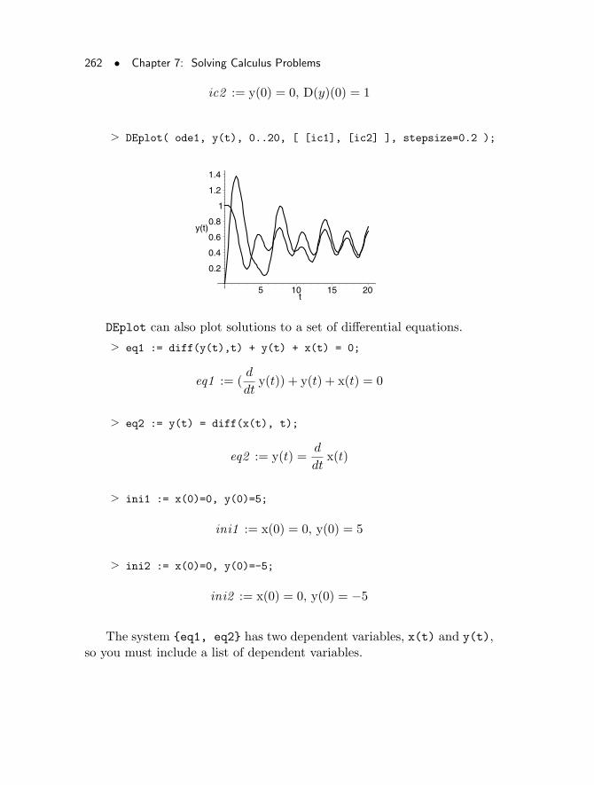
262 • Chapter 7: Solving Calculus Problems
ic2 := y(0) = 0, D(y)(0) = 1
> DEplot( ode1, y(t), 0..20, [ [ic1], [ic2] ], stepsize=0.2 );
0.2
0.4
0.6
0.8
1
1.2
1.4
y(t)
5 10 15 20t
DEplot can also plot solutions to a set of differential equations.
> eq1 := diff(y(t),t) + y(t) + x(t) = 0;
eq1 := (d
dty(t)) + y(t) + x(t) = 0
> eq2 := y(t) = diff(x(t), t);
eq2 := y(t) =d
dtx(t)
> ini1 := x(0)=0, y(0)=5;
ini1 := x(0) = 0, y(0) = 5
> ini2 := x(0)=0, y(0)=-5;
ini2 := x(0) = 0, y(0) = −5
The system {eq1, eq2} has two dependent variables, x(t) and y(t),so you must include a list of dependent variables.
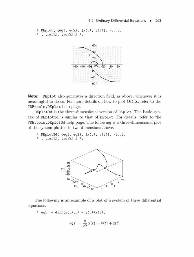
7.2 Ordinary Differential Equations • 263
> DEplot( {eq1, eq2}, [x(t), y(t)], -5..5,> [ [ini1], [ini2] ] );
–60
–40
–20
0
20
40
60
y
–60 –40 –20 20 40 60x
Note: DEplot also generates a direction field, as above, whenever it ismeaningful to do so. For more details on how to plot ODEs, refer to the?DEtools,DEplot help page.
DEplot3d is the three-dimensional version of DEplot. The basic syn-tax of DEplot3d is similar to that of DEplot. For details, refer to the?DEtools,DEplot3d help page. The following is a three-dimensional plotof the system plotted in two dimensions above.
> DEplot3d( {eq1, eq2}, [x(t), y(t)], -5..5,> [ [ini1], [ini2] ] );
–4–2
02
4t
–60–40
–200
2040
60x(t)
–40–20
02040
y(t)
The following is an example of a plot of a system of three differentialequations.
> eq1 := diff(x(t),t) = y(t)+z(t);
eq1 :=d
dtx(t) = y(t) + z(t)
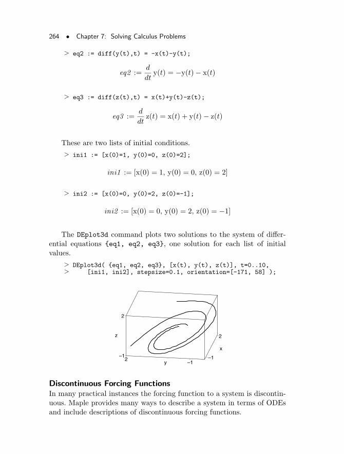
264 • Chapter 7: Solving Calculus Problems
> eq2 := diff(y(t),t) = -x(t)-y(t);
eq2 :=d
dty(t) = −y(t)− x(t)
> eq3 := diff(z(t),t) = x(t)+y(t)-z(t);
eq3 :=d
dtz(t) = x(t) + y(t)− z(t)
These are two lists of initial conditions.
> ini1 := [x(0)=1, y(0)=0, z(0)=2];
ini1 := [x(0) = 1, y(0) = 0, z(0) = 2]
> ini2 := [x(0)=0, y(0)=2, z(0)=-1];
ini2 := [x(0) = 0, y(0) = 2, z(0) = −1]
The DEplot3d command plots two solutions to the system of differ-ential equations {eq1, eq2, eq3}, one solution for each list of initialvalues.
> DEplot3d( {eq1, eq2, eq3}, [x(t), y(t), z(t)], t=0..10,> [ini1, ini2], stepsize=0.1, orientation=[-171, 58] );
–1
2
x
–12
y–1
2
z
Discontinuous Forcing FunctionsIn many practical instances the forcing function to a system is discontin-uous. Maple provides many ways to describe a system in terms of ODEsand include descriptions of discontinuous forcing functions.
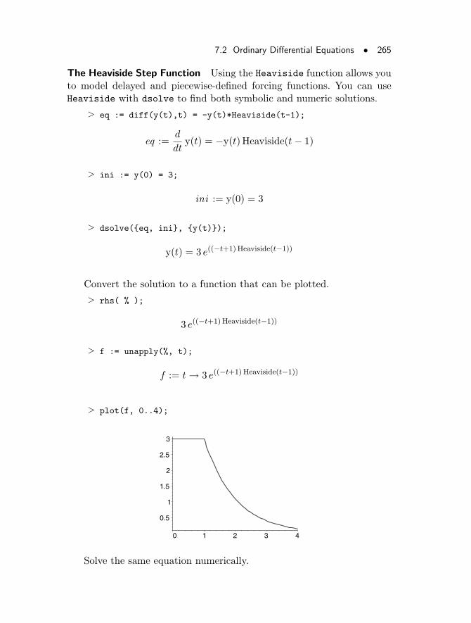
7.2 Ordinary Differential Equations • 265
The Heaviside Step Function Using the Heaviside function allows youto model delayed and piecewise-defined forcing functions. You can useHeaviside with dsolve to find both symbolic and numeric solutions.
> eq := diff(y(t),t) = -y(t)*Heaviside(t-1);
eq :=d
dty(t) = −y(t)Heaviside(t− 1)
> ini := y(0) = 3;
ini := y(0) = 3
> dsolve({eq, ini}, {y(t)});
y(t) = 3 e((−t+1)Heaviside(t−1))
Convert the solution to a function that can be plotted.
> rhs( % );
3 e((−t+1)Heaviside(t−1))
> f := unapply(%, t);
f := t → 3 e((−t+1)Heaviside(t−1))
> plot(f, 0..4);
0.5
1
1.5
2
2.5
3
0 1 2 3 4
Solve the same equation numerically.
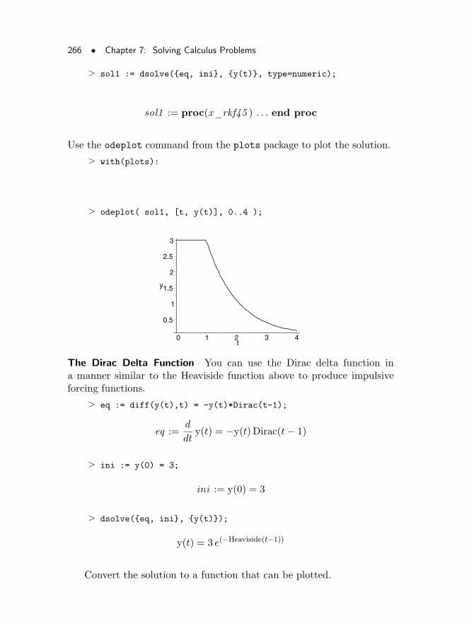
266 • Chapter 7: Solving Calculus Problems
> sol1 := dsolve({eq, ini}, {y(t)}, type=numeric);
sol1 := proc(x_rkf45 ) . . . end proc
Use the odeplot command from the plots package to plot the solution.
> with(plots):
> odeplot( sol1, [t, y(t)], 0..4 );
0.5
1
1.5
2
2.5
3
y
0 1 2 3 4t
The Dirac Delta Function You can use the Dirac delta function ina manner similar to the Heaviside function above to produce impulsiveforcing functions.
> eq := diff(y(t),t) = -y(t)*Dirac(t-1);
eq :=d
dty(t) = −y(t)Dirac(t− 1)
> ini := y(0) = 3;
ini := y(0) = 3
> dsolve({eq, ini}, {y(t)});
y(t) = 3 e(−Heaviside(t−1))
Convert the solution to a function that can be plotted.
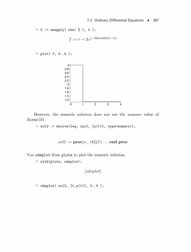
7.2 Ordinary Differential Equations • 267
> f := unapply( rhs( % ), t );
f := t → 3 e(−Heaviside(t−1))
> plot( f, 0..4 );
1.21.41.61.8
22.22.42.62.8
3
0 1 2 3 4
However, the numeric solution does not see the nonzero value ofDirac(0).
> sol2 := dsolve({eq, ini}, {y(t)}, type=numeric);
sol2 := proc(x_rkf45 ) . . . end proc
Use odeplot from plots to plot the numeric solution.
> with(plots, odeplot);
[odeplot ]
> odeplot( sol2, [t,y(t)], 0..4 );
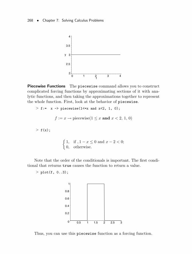
268 • Chapter 7: Solving Calculus Problems
2
2.5
3
3.5
4
y
0 1 2 3 4t
Piecewise Functions The piecewise command allows you to constructcomplicated forcing functions by approximating sections of it with ana-lytic functions, and then taking the approximations together to representthe whole function. First, look at the behavior of piecewise.
> f:= x -> piecewise(1<=x and x<2, 1, 0);
f := x → piecewise(1 ≤ x and x < 2, 1, 0)
> f(x);
{
1, if , 1− x ≤ 0 and x− 2 < 0;0, otherwise.
Note that the order of the conditionals is important. The first condi-tional that returns true causes the function to return a value.
> plot(f, 0..3);
0
0.2
0.4
0.6
0.8
1
0.5 1 1.5 2 2.5 3
Thus, you can use this piecewise function as a forcing function.
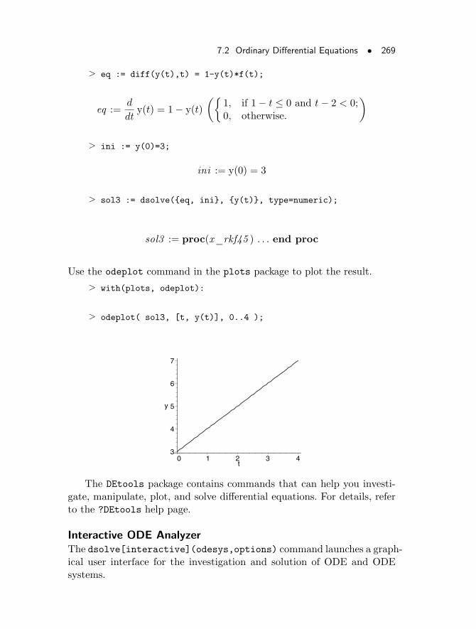
7.2 Ordinary Differential Equations • 269
> eq := diff(y(t),t) = 1-y(t)*f(t);
eq :=d
dty(t) = 1− y(t)
({
1, if 1− t ≤ 0 and t− 2 < 0;0, otherwise.
)
> ini := y(0)=3;
ini := y(0) = 3
> sol3 := dsolve({eq, ini}, {y(t)}, type=numeric);
sol3 := proc(x_rkf45 ) . . . end proc
Use the odeplot command in the plots package to plot the result.
> with(plots, odeplot):
> odeplot( sol3, [t, y(t)], 0..4 );
3
4
5
6
7
y
0 1 2 3 4t
The DEtools package contains commands that can help you investi-gate, manipulate, plot, and solve differential equations. For details, referto the ?DEtools help page.
Interactive ODE AnalyzerThe dsolve[interactive](odesys,options) command launches a graph-ical user interface for the investigation and solution of ODE and ODEsystems.
270 • Chapter 7: Solving Calculus Problems
If odesys is not given in the call to dsolve[interactive], thenodesys can be entered by using the interface; otherwise, the input equa-tions are examined and used as a starting point for the application (theseequations can be changed from within the graphical user interface).
For details about the command and interface, see ?dsolve,interactiveand ?worksheet,interactive,dsolveinterface.
7.3 Partial Differential Equations
Partial differential equations (PDEs) are in general very difficult to solve.Maple provides a number of commands for solving, manipulating, andplotting PDEs. Some of these commands are in the standard library, butmost of them reside in the PDEtools package.
The pdsolve CommandThe pdsolve command can solve many partial differential equations. Thisis the basic syntax of the pdsolve command.
pdsolve( pde, var )
• pde is the partial differential equation
• var is the variable with respect to which pdsolve solves
The following is the one-dimensional wave equation.
> wave := diff(u(x,t), t,t) - c^2 * diff(u(x,t), x,x);
wave := (∂2
∂t2u(x, t))− c2 (
∂2
∂x2u(x, t))
To solve for u(x,t), first load the PDEtools package.
> with(PDEtools):> sol := pdsolve( wave, u(x,t) );
sol := u(x, t) = _F1(c t+ x) + _F2(c t− x)
Note the solution is in terms of two arbitrary functions, _F1 and _F2.To plot the solution you need a particular set of functions.
7.3 Partial Differential Equations • 271
> f1 := xi -> exp(-xi^2);
f1 := ξ → e(−ξ2)
> f2 := xi -> piecewise(-1/2<xi and xi<1/2, 1, 0);
f2 := ξ → piecewise(−1
2< ξ and ξ <
1
2, 1, 0)
Substitute these functions into the solution.
> eval( sol, {_F1=f1, _F2=f2, c=1} );
u(x, t) = e(−(t+x)2) +
({
1 −t+ x <1
2and t− x <
1
20 otherwise
)
Use the rhs command to select the solution.
> rhs(%);
e(−(t+x)2) +
({
1 −t+ x <1
2and t− x <
1
20 otherwise
)
The unapply command converts the expression to a function.
> f := unapply(%, x,t);
f := (x, t) →
e(−(t+x)2) + piecewise(−t+ x <1
2and t− x <
1
2, 1, 0)
Plot the solution.
> plot3d( f, -8..8, 0..5, grid=[40,40] );
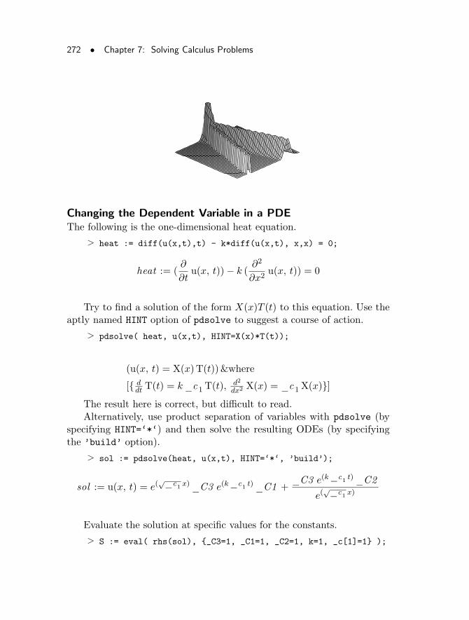
272 • Chapter 7: Solving Calculus Problems
Changing the Dependent Variable in a PDEThe following is the one-dimensional heat equation.
> heat := diff(u(x,t),t) - k*diff(u(x,t), x,x) = 0;
heat := (∂
∂tu(x, t))− k (
∂2
∂x2u(x, t)) = 0
Try to find a solution of the form X(x)T (t) to this equation. Use theaptly named HINT option of pdsolve to suggest a course of action.
> pdsolve( heat, u(x,t), HINT=X(x)*T(t));
(u(x, t) = X(x) T(t))&where
[{ ddt T(t) = k_c1T(t),
d2
dx2 X(x) = _c1X(x)}]
The result here is correct, but difficult to read.Alternatively, use product separation of variables with pdsolve (by
specifying HINT=‘*‘) and then solve the resulting ODEs (by specifyingthe ’build’ option).
> sol := pdsolve(heat, u(x,t), HINT=‘*‘, ’build’);
sol := u(x, t) = e(√_c1 x)_C3 e(k_c1 t)_C1 +
_C3 e(k_c1 t)_C2
e(√_c1 x)
Evaluate the solution at specific values for the constants.
> S := eval( rhs(sol), {_C3=1, _C1=1, _C2=1, k=1, _c[1]=1} );
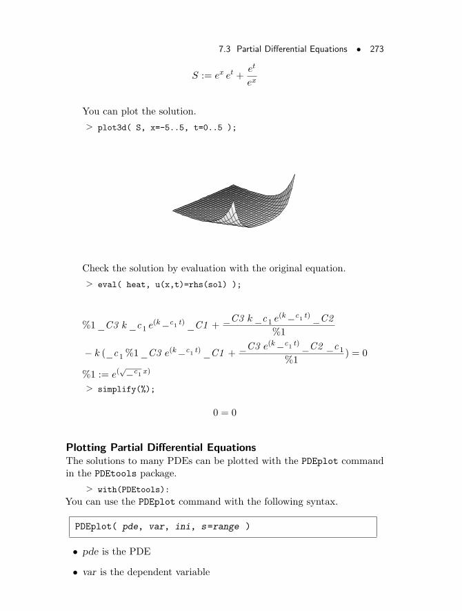
7.3 Partial Differential Equations • 273
S := ex et +et
ex
You can plot the solution.
> plot3d( S, x=-5..5, t=0..5 );
Check the solution by evaluation with the original equation.
> eval( heat, u(x,t)=rhs(sol) );
%1_C3 k_c1 e(k_c1 t)_C1 +
_C3 k_c1 e(k_c1 t)_C2
%1
− k (_c1%1_C3 e(k_c1 t)_C1 +_C3 e(k_c1 t)_C2 _c1
%1) = 0
%1 := e(√_c1 x)
> simplify(%);
0 = 0
Plotting Partial Differential EquationsThe solutions to many PDEs can be plotted with the PDEplot commandin the PDEtools package.
> with(PDEtools):
You can use the PDEplot command with the following syntax.
PDEplot( pde, var, ini, s=range )
• pde is the PDE
• var is the dependent variable
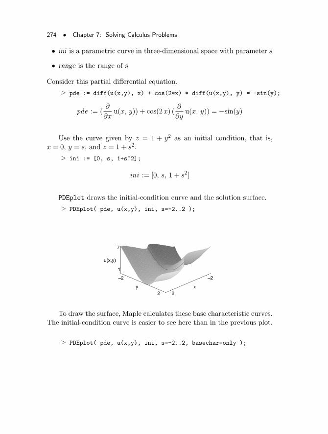
274 • Chapter 7: Solving Calculus Problems
• ini is a parametric curve in three-dimensional space with parameter s
• range is the range of s
Consider this partial differential equation.
> pde := diff(u(x,y), x) + cos(2*x) * diff(u(x,y), y) = -sin(y);
pde := (∂
∂xu(x, y)) + cos(2x) (
∂
∂yu(x, y)) = −sin(y)
Use the curve given by z = 1 + y2 as an initial condition, that is,x = 0, y = s, and z = 1 + s2.
> ini := [0, s, 1+s^2];
ini := [0, s, 1 + s2]
PDEplot draws the initial-condition curve and the solution surface.
> PDEplot( pde, u(x,y), ini, s=-2..2 );
–2
2x
–2
2y
1
7
u(x,y)
To draw the surface, Maple calculates these base characteristic curves.The initial-condition curve is easier to see here than in the previous plot.
> PDEplot( pde, u(x,y), ini, s=-2..2, basechar=only );
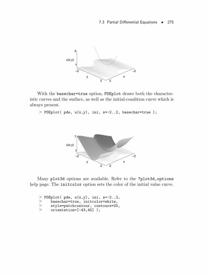
7.3 Partial Differential Equations • 275
–2
2x
–2
2y
1
5
u(x,y)
With the basechar=true option, PDEplot draws both the character-istic curves and the surface, as well as the initial-condition curve which isalways present.
> PDEplot( pde, u(x,y), ini, s=-2..2, basechar=true );
–2
2x
–2
2y
1
7
u(x,y)
Many plot3d options are available. Refer to the ?plot3d,options
help page. The initcolor option sets the color of the initial value curve.
> PDEplot( pde, u(x,y), ini, s=-2..2,> basechar=true, initcolor=white,> style=patchcontour, contours=20,> orientation=[-43,45] );
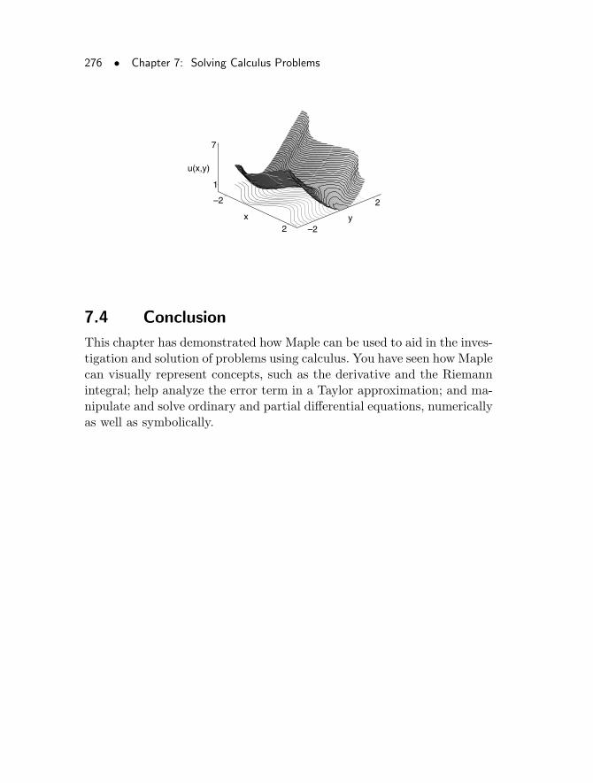
276 • Chapter 7: Solving Calculus Problems
–2
2x
–2
2
y
1
7
u(x,y)
7.4 Conclusion
This chapter has demonstrated how Maple can be used to aid in the inves-tigation and solution of problems using calculus. You have seen how Maplecan visually represent concepts, such as the derivative and the Riemannintegral; help analyze the error term in a Taylor approximation; and ma-nipulate and solve ordinary and partial differential equations, numericallyas well as symbolically.
8 Input and Output
Maple provides convenient ways to import and export raw numerical dataand graphics. It presents individual algebraic and numeric results in for-mats suitable for use in FORTRAN, C, or the mathematical typesettingsystem LATEX. You can export the entire worksheet as a file in any of thefollowing formats: HTML or HTML with MathML, LATEX, Maple Input,Maple Text, Maplet application, Plain Text, or Rich Text Format. Youcan cut and paste results, and export either single expressions or entireworksheets.
This chapter discusses the most common aspects of exporting andimporting information to and from files. It introduces how Maple inter-acts with the file system on your computer, and how Maple can begininteracting with other software.
In This Chapter• Reading Files
• Writing Data to a File
• Exporting Worksheets
• Printing Graphics
8.1 Reading Files
The two most common cases for reading files are to obtain data and toretrieve Maple commands stored in a text file.
• The first case is often concerned with data generated from an ex-periment. You can store numbers separated by whitespace and linebreaks in a text file, then read them into Maple for study. You can
277
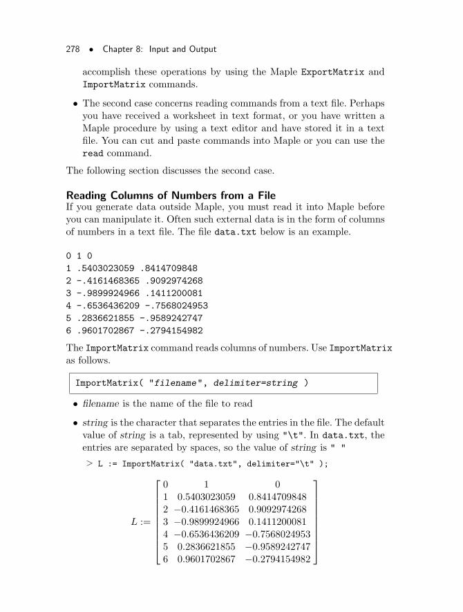
278 • Chapter 8: Input and Output
accomplish these operations by using the Maple ExportMatrix andImportMatrix commands.
• The second case concerns reading commands from a text file. Perhapsyou have received a worksheet in text format, or you have written aMaple procedure by using a text editor and have stored it in a textfile. You can cut and paste commands into Maple or you can use theread command.
The following section discusses the second case.
Reading Columns of Numbers from a FileIf you generate data outside Maple, you must read it into Maple beforeyou can manipulate it. Often such external data is in the form of columnsof numbers in a text file. The file data.txt below is an example.
0 1 0
1 .5403023059 .8414709848
2 -.4161468365 .9092974268
3 -.9899924966 .1411200081
4 -.6536436209 -.7568024953
5 .2836621855 -.9589242747
6 .9601702867 -.2794154982
The ImportMatrix command reads columns of numbers. Use ImportMatrixas follows.
ImportMatrix( "filename", delimiter=string )
• filename is the name of the file to read
• string is the character that separates the entries in the file. The defaultvalue of string is a tab, represented by using "\t". In data.txt, theentries are separated by spaces, so the value of string is " "
> L := ImportMatrix( "data.txt", delimiter="\t" );
L :=
0 1 01 0.5403023059 0.84147098482 −0.4161468365 0.90929742683 −0.9899924966 0.14112000814 −0.6536436209 −0.75680249535 0.2836621855 −0.95892427476 0.9601702867 −0.2794154982
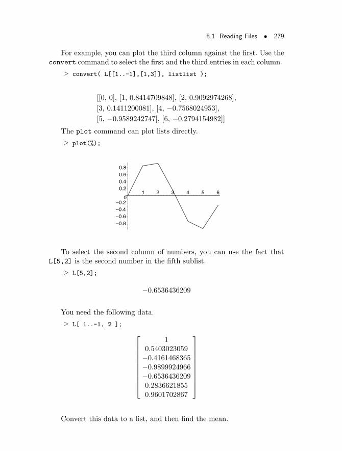
8.1 Reading Files • 279
For example, you can plot the third column against the first. Use theconvert command to select the first and the third entries in each column.
> convert( L[[1..-1],[1,3]], listlist );
[[0, 0], [1, 0.8414709848], [2, 0.9092974268],
[3, 0.1411200081], [4, −0.7568024953],
[5, −0.9589242747], [6, −0.2794154982]]
The plot command can plot lists directly.
> plot(%);
–0.8–0.6–0.4–0.2
0
0.20.40.60.8
1 2 3 4 5 6
To select the second column of numbers, you can use the fact thatL[5,2] is the second number in the fifth sublist.
> L[5,2];
−0.6536436209
You need the following data.
> L[ 1..-1, 2 ];
10.5403023059−0.4161468365−0.9899924966−0.65364362090.28366218550.9601702867
Convert this data to a list, and then find the mean.
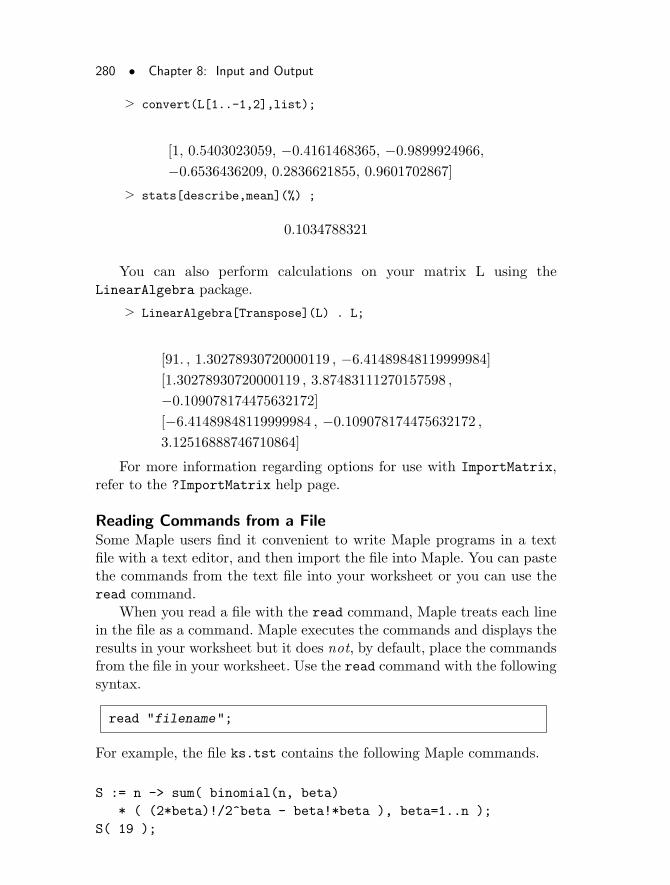
280 • Chapter 8: Input and Output
> convert(L[1..-1,2],list);
[1, 0.5403023059, −0.4161468365, −0.9899924966,
−0.6536436209, 0.2836621855, 0.9601702867]
> stats[describe,mean](%) ;
0.1034788321
You can also perform calculations on your matrix L using theLinearAlgebra package.
> LinearAlgebra[Transpose](L) . L;
[91. , 1.30278930720000119 , −6.41489848119999984]
[1.30278930720000119 , 3.87483111270157598 ,
−0.109078174475632172]
[−6.41489848119999984 , −0.109078174475632172 ,
3.12516888746710864]
For more information regarding options for use with ImportMatrix,refer to the ?ImportMatrix help page.
Reading Commands from a FileSome Maple users find it convenient to write Maple programs in a textfile with a text editor, and then import the file into Maple. You can pastethe commands from the text file into your worksheet or you can use theread command.
When you read a file with the read command, Maple treats each linein the file as a command. Maple executes the commands and displays theresults in your worksheet but it does not, by default, place the commandsfrom the file in your worksheet. Use the read command with the followingsyntax.
read "filename";
For example, the file ks.tst contains the following Maple commands.
S := n -> sum( binomial(n, beta)
* ( (2*beta)!/2^beta - beta!*beta ), beta=1..n );
S( 19 );
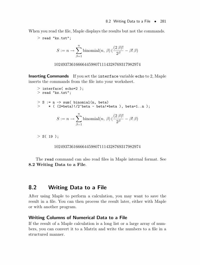
8.2 Writing Data to a File • 281
When you read the file, Maple displays the results but not the commands.
> read "ks.tst";
S := n →n∑
β=1
binomial(n, β) ((2β)!
2β− β!β)
1024937361666644598071114328769317982974
Inserting Commands If you set the interface variable echo to 2, Mapleinserts the commands from the file into your worksheet.
> interface( echo=2 );> read "ks.tst";
> S := n -> sum( binomial(n, beta)> * ( (2*beta)!/2^beta - beta!*beta ), beta=1..n );
S := n →n∑
β=1
binomial(n, β) ((2β)!
2β− β!β)
> S( 19 );
1024937361666644598071114328769317982974
The read command can also read files in Maple internal format. See8.2 Writing Data to a File.
8.2 Writing Data to a File
After using Maple to perform a calculation, you may want to save theresult in a file. You can then process the result later, either with Mapleor with another program.
Writing Columns of Numerical Data to a FileIf the result of a Maple calculation is a long list or a large array of num-bers, you can convert it to a Matrix and write the numbers to a file in astructured manner.
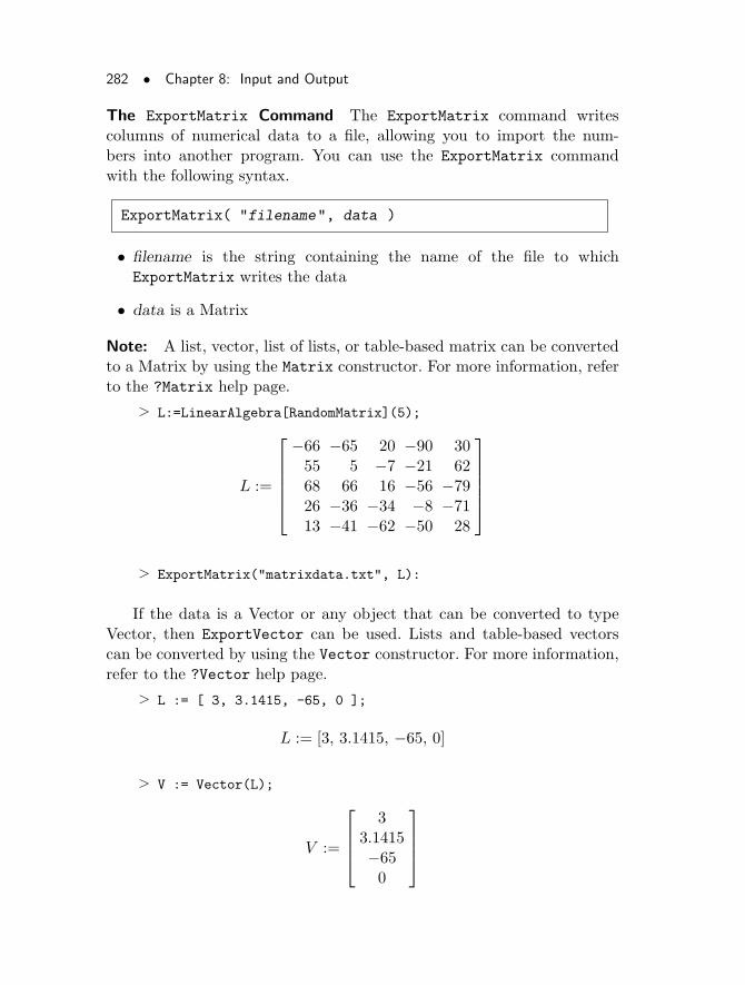
282 • Chapter 8: Input and Output
The ExportMatrix Command The ExportMatrix command writescolumns of numerical data to a file, allowing you to import the num-bers into another program. You can use the ExportMatrix commandwith the following syntax.
ExportMatrix( "filename", data )
• filename is the string containing the name of the file to whichExportMatrix writes the data
• data is a Matrix
Note: A list, vector, list of lists, or table-based matrix can be convertedto a Matrix by using the Matrix constructor. For more information, referto the ?Matrix help page.
> L:=LinearAlgebra[RandomMatrix](5);
L :=
−66 −65 20 −90 3055 5 −7 −21 6268 66 16 −56 −7926 −36 −34 −8 −7113 −41 −62 −50 28
> ExportMatrix("matrixdata.txt", L):
If the data is a Vector or any object that can be converted to typeVector, then ExportVector can be used. Lists and table-based vectorscan be converted by using the Vector constructor. For more information,refer to the ?Vector help page.
> L := [ 3, 3.1415, -65, 0 ];
L := [3, 3.1415, −65, 0]
> V := Vector(L);
V :=
33.1415−650
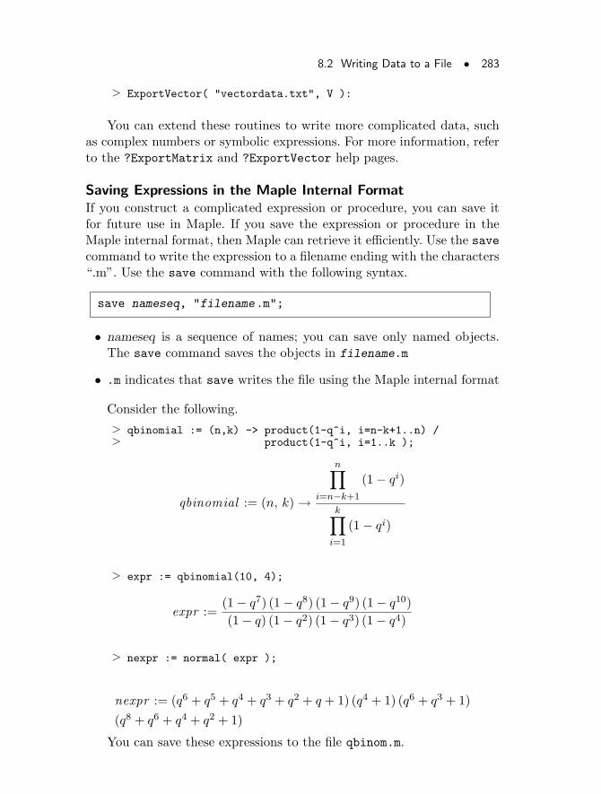
8.2 Writing Data to a File • 283
> ExportVector( "vectordata.txt", V ):
You can extend these routines to write more complicated data, suchas complex numbers or symbolic expressions. For more information, referto the ?ExportMatrix and ?ExportVector help pages.
Saving Expressions in the Maple Internal FormatIf you construct a complicated expression or procedure, you can save itfor future use in Maple. If you save the expression or procedure in theMaple internal format, then Maple can retrieve it efficiently. Use the savecommand to write the expression to a filename ending with the characters“.m”. Use the save command with the following syntax.
save nameseq, "filename.m";
• nameseq is a sequence of names; you can save only named objects.The save command saves the objects in filename.m
• .m indicates that save writes the file using the Maple internal format
Consider the following.
> qbinomial := (n,k) -> product(1-q^i, i=n-k+1..n) /> product(1-q^i, i=1..k );
qbinomial := (n, k) →
n∏
i=n−k+1
(1− qi)
k∏
i=1
(1− qi)
> expr := qbinomial(10, 4);
expr :=(1− q7) (1− q8) (1− q9) (1− q10)
(1− q) (1− q2) (1− q3) (1− q4)
> nexpr := normal( expr );
nexpr := (q6 + q5 + q4 + q3 + q2 + q + 1) (q4 + 1) (q6 + q3 + 1)
(q8 + q6 + q4 + q2 + 1)
You can save these expressions to the file qbinom.m.
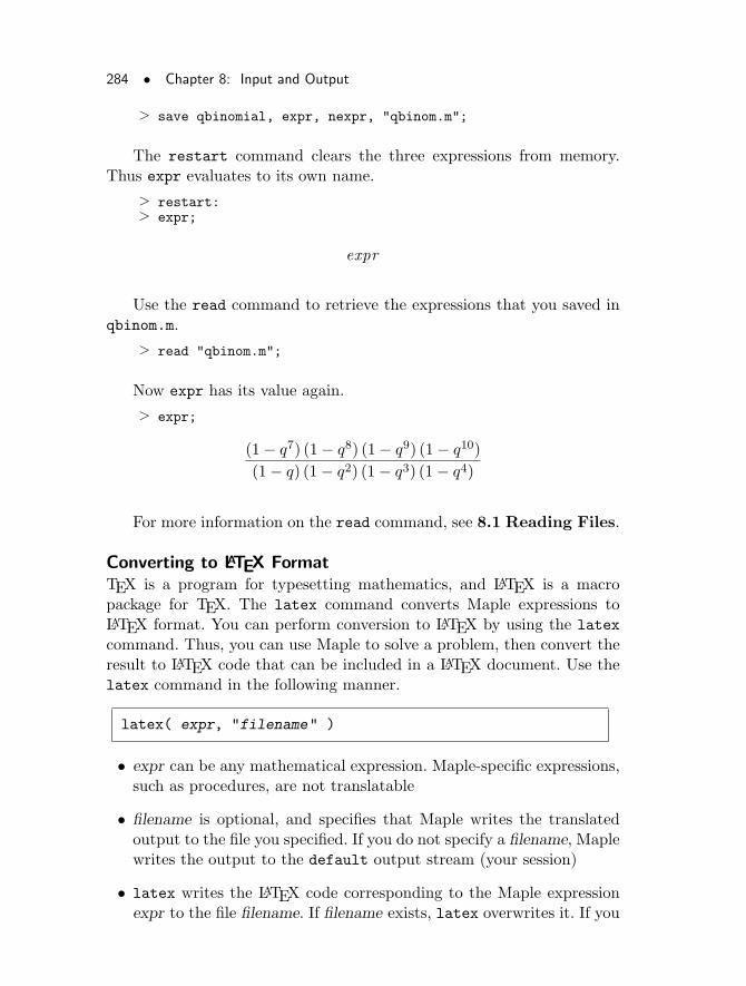
284 • Chapter 8: Input and Output
> save qbinomial, expr, nexpr, "qbinom.m";
The restart command clears the three expressions from memory.Thus expr evaluates to its own name.
> restart:> expr;
expr
Use the read command to retrieve the expressions that you saved inqbinom.m.
> read "qbinom.m";
Now expr has its value again.
> expr;
(1− q7) (1− q8) (1− q9) (1− q10)
(1− q) (1− q2) (1− q3) (1− q4)
For more information on the read command, see 8.1 Reading Files.
Converting to LATEX FormatTEX is a program for typesetting mathematics, and LATEX is a macropackage for TEX. The latex command converts Maple expressions toLATEX format. You can perform conversion to LATEX by using the latex
command. Thus, you can use Maple to solve a problem, then convert theresult to LATEX code that can be included in a LATEX document. Use thelatex command in the following manner.
latex( expr, "filename" )
• expr can be any mathematical expression. Maple-specific expressions,such as procedures, are not translatable
• filename is optional, and specifies that Maple writes the translatedoutput to the file you specified. If you do not specify a filename, Maplewrites the output to the default output stream (your session)
• latex writes the LATEX code corresponding to the Maple expressionexpr to the file filename. If filename exists, latex overwrites it. If you
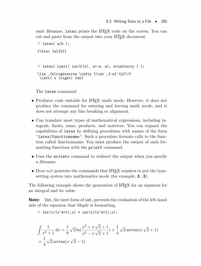
8.2 Writing Data to a File • 285
omit filename, latex prints the LATEX code on the screen. You cancut and paste from the output into your LATEX document.
> latex( a/b );
{\frac {a}{b}}
> latex( Limit( int(f(x), x=-n..n), n=infinity ) );
\lim _{n\rightarrow \infty }\int _{-n}^{n}\!f\left( x \right) {dx}
The latex command:
• Produces code suitable for LATEX math mode. However, it does notproduce the command for entering and leaving math mode, and itdoes not attempt any line breaking or alignment.
• Can translate most types of mathematical expressions, including in-tegrals, limits, sums, products, and matrices. You can expand thecapabilities of latex by defining procedures with names of the form‘latex/functionname‘. Such a procedure formats calls to the func-tion called functionname. You must produce the output of such for-matting functions with the printf command.
• Uses the writeto command to redirect the output when you specifya filename.
• Does not generate the commands that LATEX requires to put the type-setting system into mathematics mode (for example, $...$).
The following example shows the generation of LATEX for an equation foran integral and its value.
Note: Int, the inert form of int, prevents the evaluation of the left-handside of the equation that Maple is formatting.
> Int(1/(x^4+1),x) = int(1/(x^4+1),x);
∫
1
x4 + 1dx =
1
8
√2 ln(
x2 + x√2 + 1
x2 − x√2 + 1
) +1
4
√2 arctan(x
√2 + 1)
+1
4
√2 arctan(x
√2− 1)
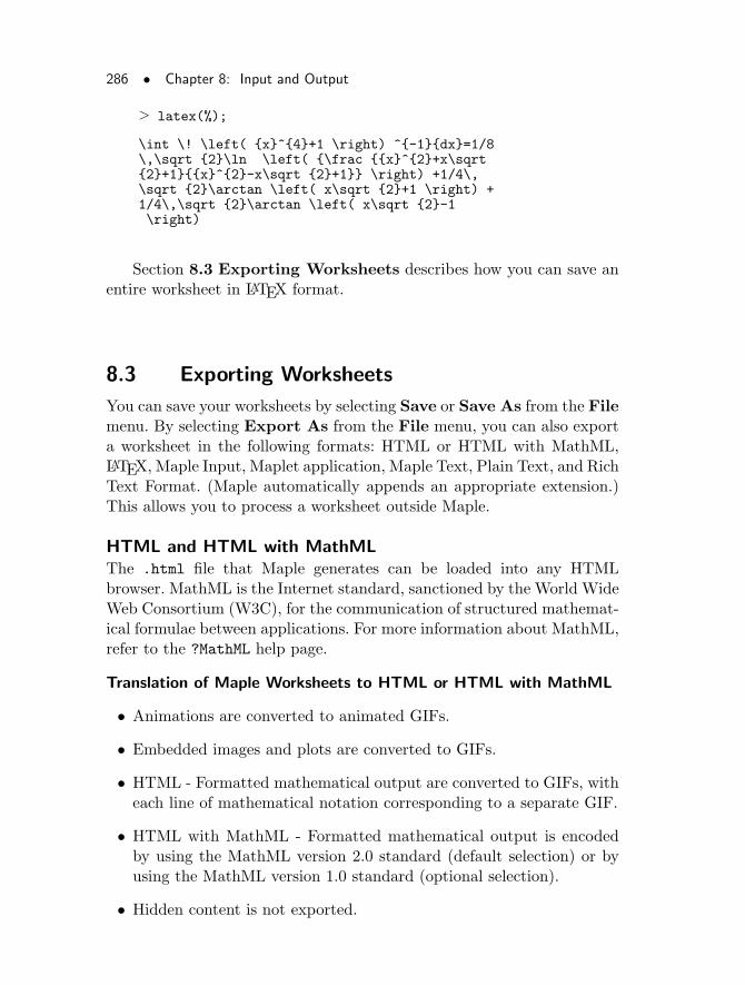
286 • Chapter 8: Input and Output
> latex(%);
\int \! \left( {x}^{4}+1 \right) ^{-1}{dx}=1/8\,\sqrt {2}\ln \left( {\frac {{x}^{2}+x\sqrt{2}+1}{{x}^{2}-x\sqrt {2}+1}} \right) +1/4\,\sqrt {2}\arctan \left( x\sqrt {2}+1 \right) +1/4\,\sqrt {2}\arctan \left( x\sqrt {2}-1\right)
Section 8.3 Exporting Worksheets describes how you can save anentire worksheet in LATEX format.
8.3 Exporting Worksheets
You can save your worksheets by selecting Save or Save As from the Filemenu. By selecting Export As from the File menu, you can also exporta worksheet in the following formats: HTML or HTML with MathML,LATEX, Maple Input, Maplet application, Maple Text, Plain Text, and RichText Format. (Maple automatically appends an appropriate extension.)This allows you to process a worksheet outside Maple.
HTML and HTML with MathMLThe .html file that Maple generates can be loaded into any HTMLbrowser. MathML is the Internet standard, sanctioned by the World WideWeb Consortium (W3C), for the communication of structured mathemat-ical formulae between applications. For more information about MathML,refer to the ?MathML help page.
Translation of Maple Worksheets to HTML or HTML with MathML
• Animations are converted to animated GIFs.
• Embedded images and plots are converted to GIFs.
• HTML - Formatted mathematical output are converted to GIFs, witheach line of mathematical notation corresponding to a separate GIF.
• HTML with MathML - Formatted mathematical output is encodedby using the MathML version 2.0 standard (default selection) or byusing the MathML version 1.0 standard (optional selection).
• Hidden content is not exported.
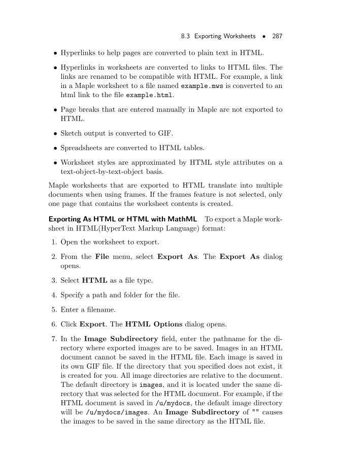
8.3 Exporting Worksheets • 287
• Hyperlinks to help pages are converted to plain text in HTML.
• Hyperlinks in worksheets are converted to links to HTML files. Thelinks are renamed to be compatible with HTML. For example, a linkin a Maple worksheet to a file named example.mws is converted to anhtml link to the file example.html.
• Page breaks that are entered manually in Maple are not exported toHTML.
• Sketch output is converted to GIF.
• Spreadsheets are converted to HTML tables.
• Worksheet styles are approximated by HTML style attributes on atext-object-by-text-object basis.
Maple worksheets that are exported to HTML translate into multipledocuments when using frames. If the frames feature is not selected, onlyone page that contains the worksheet contents is created.
Exporting As HTML or HTML with MathML To export a Maple work-sheet in HTML(HyperText Markup Language) format:
1. Open the worksheet to export.
2. From the File menu, select Export As. The Export As dialogopens.
3. Select HTML as a file type.
4. Specify a path and folder for the file.
5. Enter a filename.
6. Click Export. The HTML Options dialog opens.
7. In the Image Subdirectory field, enter the pathname for the di-rectory where exported images are to be saved. Images in an HTMLdocument cannot be saved in the HTML file. Each image is saved inits own GIF file. If the directory that you specified does not exist, itis created for you. All image directories are relative to the document.The default directory is images, and it is located under the same di-rectory that was selected for the HTML document. For example, if theHTML document is saved in /u/mydocs, the default image directorywill be /u/mydocs/images. An Image Subdirectory of "" causesthe images to be saved in the same directory as the HTML file.
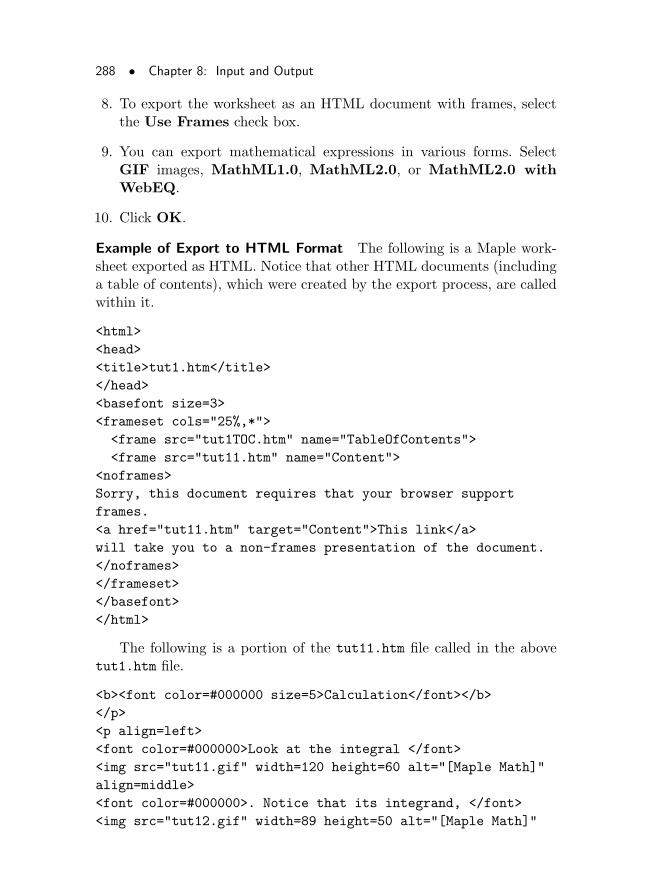
288 • Chapter 8: Input and Output
8. To export the worksheet as an HTML document with frames, selectthe Use Frames check box.
9. You can export mathematical expressions in various forms. SelectGIF images, MathML1.0, MathML2.0, or MathML2.0 withWebEQ.
10. Click OK.
Example of Export to HTML Format The following is a Maple work-sheet exported as HTML. Notice that other HTML documents (includinga table of contents), which were created by the export process, are calledwithin it.
<html>
<head>
<title>tut1.htm</title>
</head>
<basefont size=3>
<frameset cols="25%,*">
<frame src="tut1TOC.htm" name="TableOfContents">
<frame src="tut11.htm" name="Content">
<noframes>
Sorry, this document requires that your browser support
frames.
<a href="tut11.htm" target="Content">This link</a>
will take you to a non-frames presentation of the document.
</noframes>
</frameset>
</basefont>
</html>
The following is a portion of the tut11.htm file called in the abovetut1.htm file.
<b><font color=#000000 size=5>Calculation</font></b>
</p>
<p align=left>
<font color=#000000>Look at the integral </font>
<img src="tut11.gif" width=120 height=60 alt="[Maple Math]"
align=middle>
<font color=#000000>. Notice that its integrand, </font>
<img src="tut12.gif" width=89 height=50 alt="[Maple Math]"
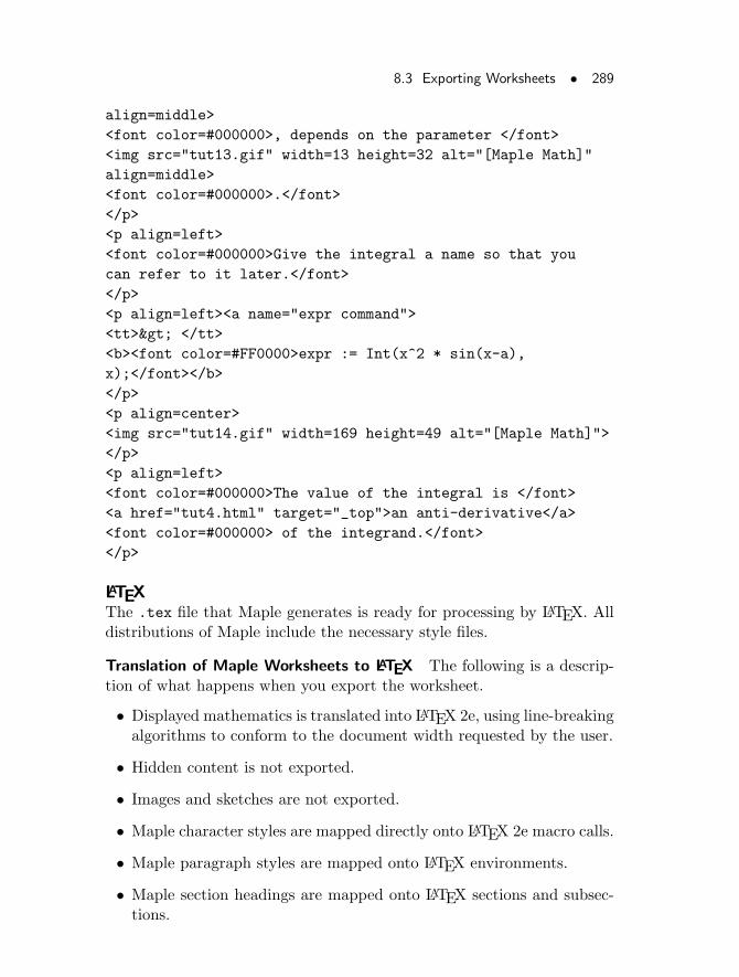
8.3 Exporting Worksheets • 289
align=middle>
<font color=#000000>, depends on the parameter </font>
<img src="tut13.gif" width=13 height=32 alt="[Maple Math]"
align=middle>
<font color=#000000>.</font>
</p>
<p align=left>
<font color=#000000>Give the integral a name so that you
can refer to it later.</font>
</p>
<p align=left><a name="expr command">
<tt>> </tt>
<b><font color=#FF0000>expr := Int(x^2 * sin(x-a),
x);</font></b>
</p>
<p align=center>
<img src="tut14.gif" width=169 height=49 alt="[Maple Math]">
</p>
<p align=left>
<font color=#000000>The value of the integral is </font>
<a href="tut4.html" target="_top">an anti-derivative</a>
<font color=#000000> of the integrand.</font>
</p>
LATEXThe .tex file that Maple generates is ready for processing by LATEX. Alldistributions of Maple include the necessary style files.
Translation of Maple Worksheets to LATEX The following is a descrip-tion of what happens when you export the worksheet.
• Displayed mathematics is translated into LATEX 2e, using line-breakingalgorithms to conform to the document width requested by the user.
• Hidden content is not exported.
• Images and sketches are not exported.
• Maple character styles are mapped directly onto LATEX 2e macro calls.
• Maple paragraph styles are mapped onto LATEX environments.
• Maple section headings are mapped onto LATEX sections and subsec-tions.
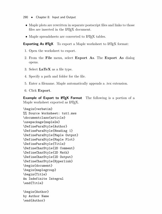
290 • Chapter 8: Input and Output
• Maple plots are rewritten in separate postscript files and links to thosefiles are inserted in the LATEX document.
• Maple spreadsheets are converted to LATEX tables.
Exporting As LATEX To export a Maple worksheet to LATEX format:
1. Open the worksheet to export.
2. From the File menu, select Export As. The Export As dialogopens.
3. Select LaTeX as a file type.
4. Specify a path and folder for the file.
5. Enter a filename. Maple automatically appends a .tex extension.
6. Click Export.
Example of Export to LATEX Format The following is a portion of aMaple worksheet exported as LATEX.
\begin{verbatim}
%% Source Worksheet: tut1.mws
\documentclass{article}
\usepackage{maple2e}
\DefineParaStyle{Author}
\DefineParaStyle{Heading 1}
\DefineParaStyle{Maple Output}
\DefineParaStyle{Maple Plot}
\DefineParaStyle{Title}
\DefineCharStyle{2D Comment}
\DefineCharStyle{2D Math}
\DefineCharStyle{2D Output}
\DefineCharStyle{Hyperlink}
\begin{document}
\begin{maplegroup}
\begin{Title}
An Indefinite Integral
\end{Title}
\begin{Author}
by Author Name
\end{Author}
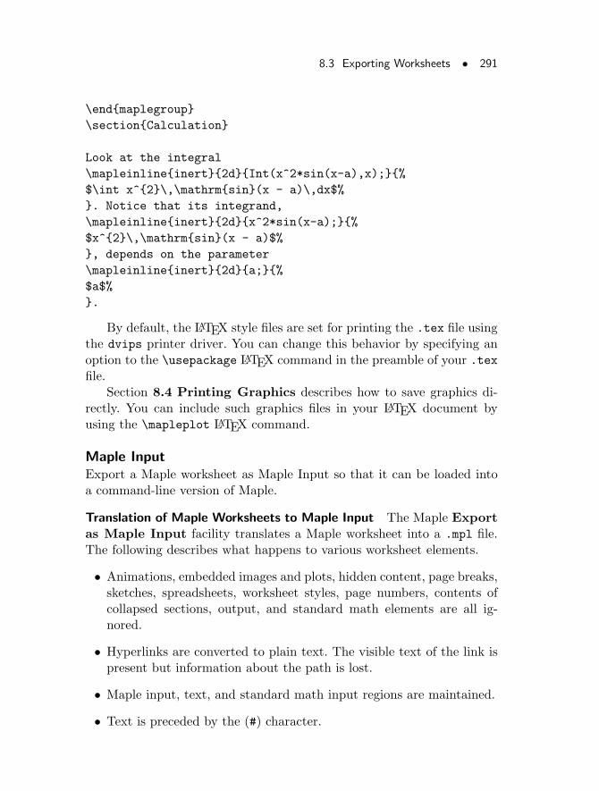
8.3 Exporting Worksheets • 291
\end{maplegroup}
\section{Calculation}
Look at the integral
\mapleinline{inert}{2d}{Int(x^2*sin(x-a),x);}{%
$\int x^{2}\,\mathrm{sin}(x - a)\,dx$%
}. Notice that its integrand,
\mapleinline{inert}{2d}{x^2*sin(x-a);}{%
$x^{2}\,\mathrm{sin}(x - a)$%
}, depends on the parameter
\mapleinline{inert}{2d}{a;}{%
$a$%
}.
By default, the LATEX style files are set for printing the .tex file usingthe dvips printer driver. You can change this behavior by specifying anoption to the \usepackage LATEX command in the preamble of your .texfile.
Section 8.4 Printing Graphics describes how to save graphics di-rectly. You can include such graphics files in your LATEX document byusing the \mapleplot LATEX command.
Maple InputExport a Maple worksheet as Maple Input so that it can be loaded intoa command-line version of Maple.
Translation of Maple Worksheets to Maple Input The Maple Exportas Maple Input facility translates a Maple worksheet into a .mpl file.The following describes what happens to various worksheet elements.
• Animations, embedded images and plots, hidden content, page breaks,sketches, spreadsheets, worksheet styles, page numbers, contents ofcollapsed sections, output, and standard math elements are all ig-nored.
• Hyperlinks are converted to plain text. The visible text of the link ispresent but information about the path is lost.
• Maple input, text, and standard math input regions are maintained.
• Text is preceded by the (#) character.
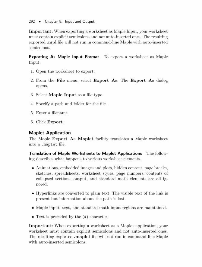
292 • Chapter 8: Input and Output
Important:When exporting a worksheet as Maple Input, your worksheetmust contain explicit semicolons and not auto-inserted ones. The resultingexported .mpl file will not run in command-line Maple with auto-insertedsemicolons.
Exporting As Maple Input Format To export a worksheet as MapleInput:
1. Open the worksheet to export.
2. From the File menu, select Export As. The Export As dialogopens.
3. Select Maple Input as a file type.
4. Specify a path and folder for the file.
5. Enter a filename.
6. Click Export.
Maplet ApplicationThe Maple Export As Maplet facility translates a Maple worksheetinto a .maplet file.
Translation of Maple Worksheets to Maplet Applications The follow-ing describes what happens to various worksheet elements.
• Animations, embedded images and plots, hidden content, page breaks,sketches, spreadsheets, worksheet styles, page numbers, contents ofcollapsed sections, output, and standard math elements are all ig-nored.
• Hyperlinks are converted to plain text. The visible text of the link ispresent but information about the path is lost.
• Maple input, text, and standard math input regions are maintained.
• Text is preceded by the (#) character.
Important: When exporting a worksheet as a Maplet application, yourworksheet must contain explicit semicolons and not auto-inserted ones.The resulting exported .maplet file will not run in command-line Maplewith auto-inserted semicolons.
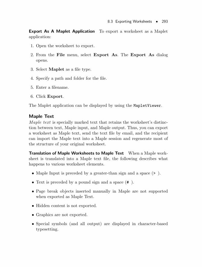
8.3 Exporting Worksheets • 293
Export As A Maplet Application To export a worksheet as a Mapletapplication:
1. Open the worksheet to export.
2. From the File menu, select Export As. The Export As dialogopens.
3. Select Maplet as a file type.
4. Specify a path and folder for the file.
5. Enter a filename.
6. Click Export.
The Maplet application can be displayed by using the MapletViewer.
Maple TextMaple text is specially marked text that retains the worksheet’s distinc-tion between text, Maple input, and Maple output. Thus, you can exporta worksheet as Maple text, send the text file by email, and the recipientcan import the Maple text into a Maple session and regenerate most ofthe structure of your original worksheet.
Translation of Maple Worksheets to Maple Text When a Maple work-sheet is translated into a Maple text file, the following describes whathappens to various worksheet elements.
• Maple Input is preceded by a greater-than sign and a space (> ).
• Text is preceded by a pound sign and a space (# ).
• Page break objects inserted manually in Maple are not supportedwhen exported as Maple Text.
• Hidden content is not exported.
• Graphics are not exported.
• Special symbols (and all output) are displayed in character-basedtypesetting.
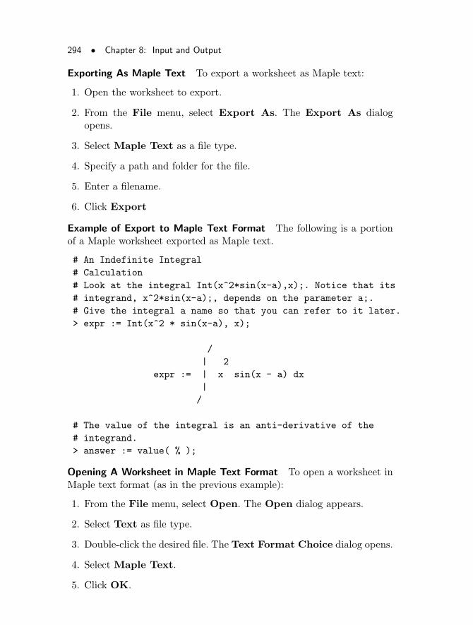
294 • Chapter 8: Input and Output
Exporting As Maple Text To export a worksheet as Maple text:
1. Open the worksheet to export.
2. From the File menu, select Export As. The Export As dialogopens.
3. Select Maple Text as a file type.
4. Specify a path and folder for the file.
5. Enter a filename.
6. Click Export
Example of Export to Maple Text Format The following is a portionof a Maple worksheet exported as Maple text.
# An Indefinite Integral
# Calculation
# Look at the integral Int(x^2*sin(x-a),x);. Notice that its
# integrand, x^2*sin(x-a);, depends on the parameter a;.
# Give the integral a name so that you can refer to it later.
> expr := Int(x^2 * sin(x-a), x);
/
| 2
expr := | x sin(x - a) dx
|
/
# The value of the integral is an anti-derivative of the
# integrand.
> answer := value( % );
Opening A Worksheet in Maple Text Format To open a worksheet inMaple text format (as in the previous example):
1. From the File menu, select Open. The Open dialog appears.
2. Select Text as file type.
3. Double-click the desired file. The Text Format Choice dialog opens.
4. Select Maple Text.
5. Click OK.
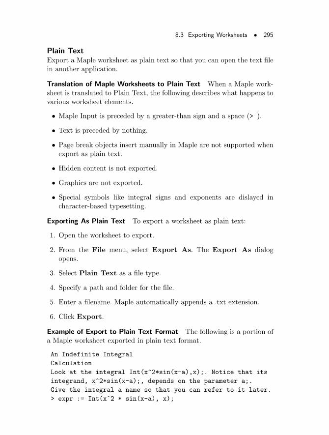
8.3 Exporting Worksheets • 295
Plain TextExport a Maple worksheet as plain text so that you can open the text filein another application.
Translation of Maple Worksheets to Plain Text When a Maple work-sheet is translated to Plain Text, the following describes what happens tovarious worksheet elements.
• Maple Input is preceded by a greater-than sign and a space (> ).
• Text is preceded by nothing.
• Page break objects insert manually in Maple are not supported whenexport as plain text.
• Hidden content is not exported.
• Graphics are not exported.
• Special symbols like integral signs and exponents are dislayed incharacter-based typesetting.
Exporting As Plain Text To export a worksheet as plain text:
1. Open the worksheet to export.
2. From the File menu, select Export As. The Export As dialogopens.
3. Select Plain Text as a file type.
4. Specify a path and folder for the file.
5. Enter a filename. Maple automatically appends a .txt extension.
6. Click Export.
Example of Export to Plain Text Format The following is a portion ofa Maple worksheet exported in plain text format.
An Indefinite Integral
Calculation
Look at the integral Int(x^2*sin(x-a),x);. Notice that its
integrand, x^2*sin(x-a);, depends on the parameter a;.
Give the integral a name so that you can refer to it later.
> expr := Int(x^2 * sin(x-a), x);
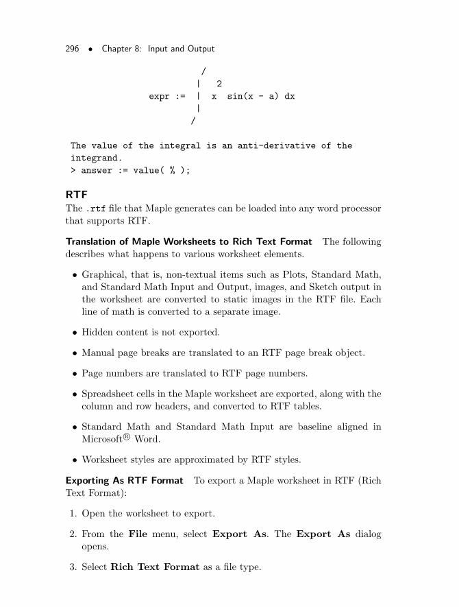
296 • Chapter 8: Input and Output
/
| 2
expr := | x sin(x - a) dx
|
/
The value of the integral is an anti-derivative of the
integrand.
> answer := value( % );
RTFThe .rtf file that Maple generates can be loaded into any word processorthat supports RTF.
Translation of Maple Worksheets to Rich Text Format The followingdescribes what happens to various worksheet elements.
• Graphical, that is, non-textual items such as Plots, Standard Math,and Standard Math Input and Output, images, and Sketch output inthe worksheet are converted to static images in the RTF file. Eachline of math is converted to a separate image.
• Hidden content is not exported.
• Manual page breaks are translated to an RTF page break object.
• Page numbers are translated to RTF page numbers.
• Spreadsheet cells in the Maple worksheet are exported, along with thecolumn and row headers, and converted to RTF tables.
• Standard Math and Standard Math Input are baseline aligned inMicrosoft r© Word.
• Worksheet styles are approximated by RTF styles.
Exporting As RTF Format To export a Maple worksheet in RTF (RichText Format):
1. Open the worksheet to export.
2. From the File menu, select Export As. The Export As dialogopens.
3. Select Rich Text Format as a file type.
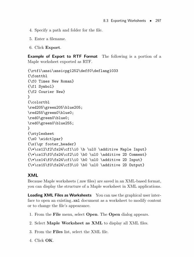
8.3 Exporting Worksheets • 297
4. Specify a path and folder for the file.
5. Enter a filename.
6. Click Export.
Example of Export to RTF Format The following is a portion of aMaple worksheet exported as RTF.
{\rtf1\ansi\ansicpg1252\deff0\deflang1033
{\fonttbl
{\f0 Times New Roman}
{\f1 Symbol}
{\f2 Courier New}
}
{\colortbl
\red205\green205\blue205;
\red255\green0\blue0;
\red0\green0\blue0;
\red0\green0\blue255;
}
{\stylesheet
{\s0 \widctlpar}
{\s1\qr footer_header}
{\*\cs12\f2\fs24\cf1\i0 \b \ul0 \additive Maple Input}
{\*\cs13\f0\fs24\cf2\i0 \b0 \ul0 \additive 2D Comment}
{\*\cs14\f0\fs24\cf1\i0 \b0 \ul0 \additive 2D Input}
{\*\cs15\f0\fs24\cf3\i0 \b0 \ul0 \additive 2D Output}
XMLBecause Maple worksheets (.mw files) are saved in an XML-based format,you can display the structure of a Maple worksheet in XML applications.
Loading XML Files as Worksheets You can use the graphical user inter-face to open an existing.xml document as a worksheet to modify contentor to change the file’s appearance.
1. From the File menu, select Open. The Open dialog appears.
2. Select Maple Worksheet as XML to display all XML files.
3. From the Files list, select the XML file.
4. Click OK.
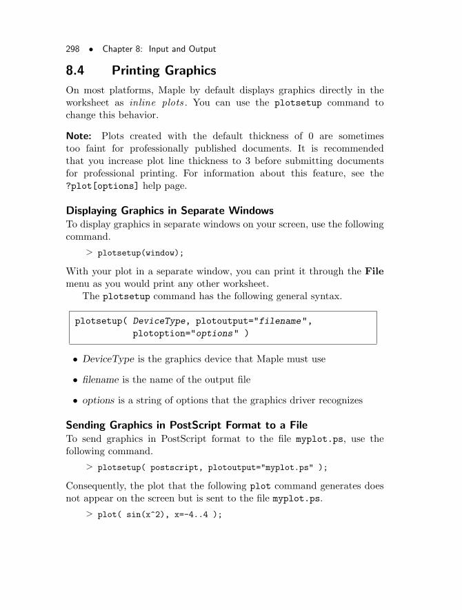
298 • Chapter 8: Input and Output
8.4 Printing Graphics
On most platforms, Maple by default displays graphics directly in theworksheet as inline plots . You can use the plotsetup command tochange this behavior.
Note: Plots created with the default thickness of 0 are sometimestoo faint for professionally published documents. It is recommendedthat you increase plot line thickness to 3 before submitting documentsfor professional printing. For information about this feature, see the?plot[options] help page.
Displaying Graphics in Separate WindowsTo display graphics in separate windows on your screen, use the followingcommand.
> plotsetup(window);
With your plot in a separate window, you can print it through the Filemenu as you would print any other worksheet.
The plotsetup command has the following general syntax.
plotsetup( DeviceType, plotoutput="filename",
plotoption="options" )
• DeviceType is the graphics device that Maple must use
• filename is the name of the output file
• options is a string of options that the graphics driver recognizes
Sending Graphics in PostScript Format to a FileTo send graphics in PostScript format to the file myplot.ps, use thefollowing command.
> plotsetup( postscript, plotoutput="myplot.ps" );
Consequently, the plot that the following plot command generates doesnot appear on the screen but is sent to the file myplot.ps.
> plot( sin(x^2), x=-4..4 );
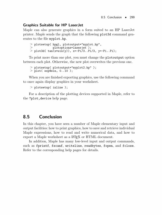
8.5 Conclusion • 299
Graphics Suitable for HP LaserJetMaple can also generate graphics in a form suited to an HP LaserJetprinter. Maple sends the graph that the following plot3d command gen-erates to the file myplot.hp.
> plotsetup( hpgl, plotoutput="myplot.hp",> plotoptions=laserjet );> plot3d( tan(x*sin(y)), x=-Pi/3..Pi/3, y=-Pi..Pi);
To print more than one plot, you must change the plotoutput optionbetween each plot. Otherwise, the new plot overwrites the previous one.
> plotsetup( plotoutput="myplot2.hp" );> plot( exp@sin, 0..10 );
When you are finished exporting graphics, use the following commandto once again display graphics in your worksheet.
> plotsetup( inline );
For a description of the plotting devices supported in Maple, refer tothe ?plot,device help page.
8.5 Conclusion
In this chapter, you have seen a number of Maple elementary input andoutput facilities: how to print graphics, how to save and retrieve individualMaple expressions, how to read and write numerical data, and how toexport a Maple worksheet as a LATEX or HTML document.
In addition, Maple has many low-level input and output commands,such as fprintf, fscanf, writeline, readbytes, fopen, and fclose.Refer to the corresponding help pages for details.

300 • Chapter 8: Input and Output
9 Maplet User InterfaceCustomization System
By using the Maplets package, you can create windows, dialogs, andother visual interfaces that interact with a user to provide the power ofMaple. Users can perform calculations, or plot functions without usingthe worksheet interface. This chapter is intended primarily for Mapletapplication users. Some information may be helpful to Maplet applicationauthors.
In This Chapter• Example Maplet
• Terminology
• How to Start the Maplets Package
• How to Invoke a Maplet Application from the Maple Worksheet
• How to Close a Maplet Application
• How to Work With Maplet Applications and the Maple Window
• How to Activate a Maplet Application Window
• How to Terminate and Restart a Maplet Application
• How to Use Graphical User Interface Shortcuts
301
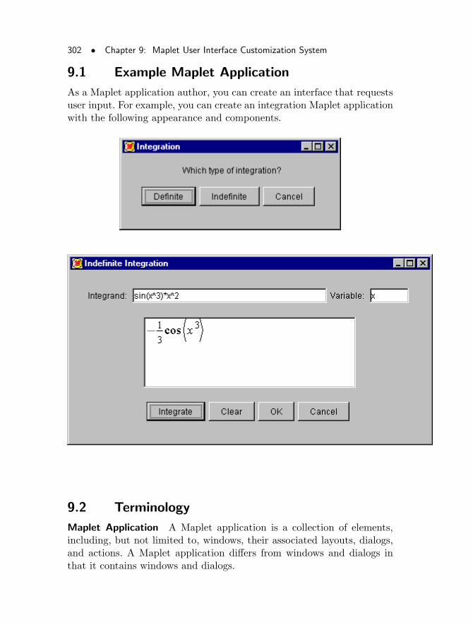
302 • Chapter 9: Maplet User Interface Customization System
9.1 Example Maplet Application
As a Maplet application author, you can create an interface that requestsuser input. For example, you can create an integration Maplet applicationwith the following appearance and components.
9.2 Terminology
Maplet Application A Maplet application is a collection of elements,including, but not limited to, windows, their associated layouts, dialogs,and actions. A Maplet application differs from windows and dialogs inthat it contains windows and dialogs.
9.3 How to Start the Maplets Package • 303
Maplet Application Author A programmer who uses Maple code towrite a Maplet application.
Maplet Application User Someone who interacts with a Maplet appli-cation.
Layout Layout defines how elements within a Maplet application aredisplayed.
Window A window is a Maplet application element. A window shouldnot be thought of as a Maplet application, but rather as one elementwithin a Maplet application. A Maplet application can contain more thanone window. Each window can contain many elements that control thelayout and function of the window.
Dialog A dialog is a Maplet application element. Unlike a window, whichcan contain elements, for example, buttons or layout elements, a dialogelement has a predefined structure. An author can specify options for adialog, but cannot add elements.
9.3 How to Start the Maplets Package
If you receive a Maple worksheet with Maplet application code, you mustfirst invoke the Maplets package. Press the Enter key after these twopossible execution groups:
> restart:> with(Maplets[Elements]);
9.4 How to Invoke a Maplet Application fromthe Maple Worksheet
To start a maplet, press the Enter key after the last colon (:), semicolon(;), or anywhere in an execution group to execute the Maplet applicationcode. In the following example, the Maplet application is written as oneexecution group. You can press Enter anywhere in the execution groupto execute the code:
304 • Chapter 9: Maplet User Interface Customization System
> mymaplet := Maplet ([> ["Hello World", Button("OK", Shutdown())]> ]):> Maplets[Display](mymaplet);
In the following example, the Maplet application is written as two ex-ecution groups. The application must be defined before using the Displaycommand.
> with(Maplets[Elements]):> my2maplet := Maplet ([> ["Hello World #2", Button("OK", Shutdown())]> ]):> Maplets[Display](my2maplet);
9.5 How to Close a Maplet Application
If the Maplet application contains a cancel button, click Cancel. Other-wise, click the appropriate Close icon for your platform. For example:
In UNIX:
1. Click the - icon in the upper left corner of the Maplet applicationwindow title bar. A drop-down list box appears.
Note: The icon varies with window manager.
2. Select Close.
In Windows:
• Click the X icon in the upper right corner of the Maplet applicationwindow title bar. The Maplet application closes.
9.6 How to Work With Maplet Applications andthe Maple Window (Modality)
When a Maplet application is running, the Maple worksheet is inaccessi-ble. If you move the cursor across the worksheet, an icon (clock in UNIX(depending on your window manager), hourglass in Windows) appears,indicating that the worksheet is inaccessible. The Maplet application mustbe closed or allowed to complete an action before the Maple worksheetcan be accessed.
9.7 How to Activate a Maplet Application Window • 305
9.7 How to Activate a Maplet ApplicationWindow
1. Click an input field in the Maplet application. The input field appearshighlighted.
2. Enter the appropriate expression, numbers, or text as required.
9.8 How to Terminate and Restart a MapletApplication
With long computations, you may choose to stop the computation.
1. To terminate the current Maplet application process, click the X (orappropriate close icon for your platform) on the Maplet applicationtitle bar.
2. To restart the terminated application, run the Maplet application byusing the lastmaplet tool.
> Maplets[Display](lastmaplet);
9.9 How to Use Graphical User InterfaceShortcuts
Drop-down List BoxesSome Maplet applications contain drop-down list boxes.
1. Enter the first character of any item in the list. The list automaticallymoves to an item that begins with the character entered.
2. Continue to enter the character until the desired selection is high-lighted.
Note that this shortcut does not apply to editable drop-down lists createdwith the ComboBox element.
306 • Chapter 9: Maplet User Interface Customization System
SPACE BAR and TAB KeyYou can use the mouse to click a Cancel or OK button in a Mapletapplication. You can also use the Tab key and Space Bar.
1. Using the Tab key, position the cursor at the Cancel or OK button.
2. Press the Space Bar. The command is entered.
9.10 Conclusion
For more information on the Maplet User Interface Customization Sys-tem, enter ?maplets at the Maple prompt or refer to the Maple Intro-ductory Programming Guide.
9.11 General Conclusion
This book aims to supply you with a good base of knowledge from whichto further explore Maple. In this role, it focuses on the interactive useof Maple. Maple is a complete language and provides complete facilitiesfor programming. The majority of Maple commands are coded in theMaple language, as this high-level, mathematically oriented language issuperior to traditional computer languages for such tasks. The MapleIntroductory Programming Guide introduces you to programming inMaple.
Index
!, 8I (
√−1), 14
π, 12~, 58%, 8->, 19:, 28:=, 18;, 6, 28?, 5$, 222_C, 76", 32@, 242, 256\, 8||, 22, 32, 211_EnvAllSolutions, 56~, 174
about, 175absolute value, 9accessing
list items, 26package commands, 80range of subexpressions, 40subexpressions, 40
accuracy, floating-point, 12–13adaptive plotting, 118add, 182adding
restrictions to solve, 47additionally, 175Advanced Programming Guide,
2algcurves, 82algebraic substitution, 41algsubs, 41, 198
animate, 128–131coords, 130, 131frames, 129, 131
animations, 217cylindrical coordinates, 132displaying, 128frames of, 129, 131, 136parametric, 2-D, 129parametric, 3-D, 131playing, 128in polar coordinates, 130in spherical coordinates, 132two-dimensional, 128
annotations, 132, 136antiderivatives, 68, 94, 232, 235applying
commands to lists (map), 38commands to multiple expres-
sions (map), 38functions to sets, 25operations to lists, 39procedures to lists, 47simplification rules, 33
approximate vs. exact results, 10–11
ApproximateInt, 93–94, 232–234,236
approximationsfloating-point, 10, 12–14series, 66
arbitrary precision integers, 8arithmetic
basic, 6exact, 10finite rings and fields, 15modulo, 15
array, 27, 28
307
308 • Index
arrays, 27–31declaring 1-D, 27declaring 2-D, 28, 29definition, 27evaluating, 30, 203mapping onto, 38printing, 28selecting elements from 1-D
arrays, 27selecting elements from 2-D
arrays, 28viewing contents, 28
arrow, 143arrow notation, 19assign, 51–53assigned, 206assigning to names, 18, 51assignment operator, 20assignments
invalid, 20multiple, 22naming, 18of sets of equations, 51valid names, 19
assume, 70, 174–177additionally, 175integer, 175nonnegative, 175
assuming, 178assumptions, 70
on names, 58, 70removing, 70, 178setting, 174–175viewing, 175
audience, 1automatic simplification, 17axes, 133, 134axis labels, 133
base n numbersconverting to, 14
basic arithmetic, 6basis, 95Bessel functions, 16binary numbers
converting to, 14binomial function, 16boundary conditions, 73
calculationsexact vs. floating point, 6
calculus, 65–71, 87, 215–240Calculus1 commands
ApproximateInt, 93–94, 232–234, 236
Hint, 90–92NewtonQuotient, 216Roots, 92Rule, 89–92Tangent, 92Understand, 90
capitalization, 12case sensitivity, 12cat, 32catastrophic cancellation, 12changing variables, 30circles, plotting, 106, 109classic worksheet, 3classical dynamics, 243coeff, 62coefficients
collecting, 61extracting, 62, 63polynomial, 62
collect, 61, 158distributed, 160
colon, 28color functions, 126combinat, 82combine, 164
expr, 37power, 37
Index • 309
combiningpowers, 37products, 37sums, 37
combstruct, 82comma delimited expressions, see
expression sequencescommand-line version, 3commands, see specific command
namesseparating, 6terminating, 6
common denominator, 36, 165complex numbers, 14complex roots, 54computations
integer, 7–9referring to previous, 8symbolic, 16
concatenation, 201, 211–213expression sequences, 22operator, 22strings, 32
conditionsinitial, 242, 274
cone, 146cones, plotting, 125conformal, 141constants, 12
factoring, 41of integration, 235
constrained scaling, in plots, 107content, multivariate polynomial,
64context, 82continuation character, 8continuity, extending by, 237contourplot, 140convert, 36, 279
base, 14binary, 14
exp, 36, 172factorial, 172hex, 14list, 36, 201, 279ln, 172parfrac, 173polynom, 200, 222rational, 173set, 36, 201sincos, 172string, 200trig, 36
convertingbetween data structures, 36between temperature scales,
36between types, 36between units, 36degrees to radians, 36expressions, 36expressions to functions, 49expressions to LATEX, 284floating-point to rational, 36radians to degrees, 36rational to partial fractions,
36series to polynomials, 36, 66,
67, 200, 222solution set to list, 46to floating-point, 13to lists, 47, 279to lists and sets, 201to strings, 200trigonometric to exponential,
36coordinates
cylindrical, 124polar, 108, 130spherical, 121viewing, 104
counting, 40
310 • Index
CurveFitting, 82, 118customer feedback, 2cutout, 148cylinderplot, 124cylindrical coordinates, 124cylindrical coordinates, animations,
132
D, 236, 242, 255data points, plotting, 116data types, 21decimal forms, 10decimal numbers, 12–14declaring arrays
one-dimensional, 27two-dimensional, 28, 29
decomposition, polynomial, 64defining
discontinuous functions, 111functions, 19functions, with arrow nota-
tion, 52functions, with unapply, 49,
72defining arrays
one-dimensional, 27two-dimensional, 28, 29
definite integrals, 69, 234degree, 62degree of polynomial, 62, 63delaying evaluation, 207denom, 39, 189denominators, 39, 189
common, 36, 165isolate, 39
densityplot, 140DEplot, 260DEplot3d, 263derivatives, 17, 68, 215
limit definition of, 216partial, 224, 237
describe, 99DESol, 259determining number of elements
(nops), 23, 25DEtools, 83dialog, see Maplet,dialogDiff, 68, 89diff, 196diffalg, 83differential equations
ordinary, 71, 241partial, 270solving, 51systems of, 76
differentiatingexpressions in a list, 38
differentiation, 17, 89difforms, 83Digits, 13digits
in floating-point calculations,default, 13
in floating-point calculations,setting, 13
in floating-point calculations,setting globally, 13
maximum length of floating-point approximations, 12
maximum length of integers,8
Dirac, 16, 73, 266Dirac delta function, 16, 73, 266discontinuous functions
defining, 111plotting, 57, 111
display, 134, 144, 217displaying
animations, 128ditto operator, 8divide, 62division
Index • 311
integer quotient, 9integer remainder, 9polynomial, 18, 61
dodecahedron, 147Domains, 83double quotes, 32dsolve, 71–77, 241
explicit, 243implicit, 243method=laplace, 244startinit, 254type=numeric, 252type=series, 249
e (exponential function), 11echo, 281eigenvalues, 97eigenvectors, 97empty_list, 26empty_set, 26equations
left-hand side, 39right-hand side, 39solving, 43, 54solving systems of, 44
error functions, 16errors
floating-point, 14relative, 12
eval, 45, 46, 62, 71, 72, 197, 202evalf, 10, 13, 216evalm, 30evaln, 206evaluating
arrays, 30, 203local variables, 206matrices, 203procedures, 203tables, 203
evaluation, 202–213and quoting, 207
and substitution, 199assigned, 206at a point, 45delayed, 207evaln, 206forcing full, 204full, 202last-name, 203levels of, 202numerical, 10, 13one-level, 206to a name, 206
exact arithmetic, 10exact numbers, analytic descrip-
tion, 12exact vs. approximate results, 10–
11exp, 12Expand, 158expand, 17, 35, 156
vs. simplify, 35–36expanded normal form, 37expanding
modulo m, 158polynomials, 35
explicit functions, plotting, 104exponential function, 11, 16exporting
as Maple text, 293as Maplet application, 292as plain text, 295HTML with MathML, 287LATEX, 290RTF, 296
ExportMatrix, 282ExportVector, 282expression sequences, 21expression trees, 192expressions
accessing subexpressions, 40
312 • Index
comma delimited, see expres-sion sequences
converting, 36converting to functions, 49exact, 6expanding, 17extracting subexpressions, 40factoring, 17identification of, 190indeterminates of, 195multiple assignments, 22multiple, applying commands
to, 38naming, 18, 51naming multiple, 22number of parts, 40operands of, 190querying contents, 193solving, assumptions, 44substituting, 30types of, 194unevaluated, 15, 207
extending by continuity, 237ExternalCalling, 83extracting
1-D array elements, 272-D array elements, 28coefficients, 62list items, 26range of subexpressions, 40set items, 46subexpressions, 40
Factor, 163factor, 17, 34
vs. solve, 63factored normal form, 36, 165factorial
integer, 9factoring, 63, 161–163
constants, 41
expressions, 17fractions, 34integers, 9modulo p, 163polynomials, 34
feasible, 102fieldplot, 141files
reading columns from, 278reading commands from, 280reading data from, 278writing columns to, 281
FileTools, 83finance, 83finding
basis, 95limits, 65roots, 43, 54–56, 58
floating-point accuracy, 12–13floating-point approximations, 12–
14maximum length, 12
floating-point arithmetic, forcing,13
floating-point conversions, 13floating-point errors, 14floating-point numbers
default accuracy of, 13vs. rational numbers, 10–11
frac, 175fractional part function, 16fractions
on common denominator, 36denominator, 39denominators of, 189expanded normal form, 37factored normal form, 36factoring, 34numerator, 39numerators of, 189on common denominator, 165
Index • 313
partial, 173fsolve, 54–56, 226
avoid, 54complex, 54limitations, 55maxsols, 54specifying range, 56
full evaluation, 202functional operator, 19functions
applying to sets, 25arguments of, 20assigning, 19Bessel, 16binomial, 16defining, 19defining with arrow notation,
52defining with unapply, 49, 72Dirac delta, 16discontinuous, plotting, 57error, 16exponential, 11, 16extending by continuity, 237fractional part, 16from expressions, 49general mathematical, 15–16Heaviside step, 16hyperbolic trigonometric, 16hypergeometric, 16inverse trigonometric, 16Legendre’s elliptic integral,
16logarithmic base 10, 16Meijer G, 16natural logarithmic, 16piecewise-defined, 268Riemann Zeta, 16round to the nearest integer,
16square root, 16
trigonometric, 16truncate to the integer part,
16
Gaussian integers, 15GaussInt, 83generating random numbers, 99genfunc, 83geom3d, 83geometry, 83Getting Started Guide, 1graphical interface
versions, 3graphical objects, 144graphics
devices, 298in separate windows, 298inline, 298printing, 298
graphing, 103three-dimensional, 119
greatest common divisor, 64of integers, 9
Groebner, 83group, 83
has, 193hastype, 194heat equation, 272Heaviside, 244, 265Heaviside step function, 16, 265help pages, accessing, 5hemisphere, 147hexidecimal numbers, converting
to, 14Hint, 90–92histograms, 100, 142HP LaserJet, 299HTML
exporting as, 287hyperbolic trigonometric functions,
16
314 • Index
hypergeometric function, 16
imaginary numbers, 14implicitplot, 138ImportMatrix, 278impulse function, 73, 266indefinite integrals, 68, 234indeterminates, 195indets, 195inequal, 139infinite domains, plotting, 105infolevel, 164, 176initial conditions, 71, 242, 274inline plots, 298Int, 68
limitations, 69integer computations, 7–9integers, 7
arbitrary precision, 8calculations with, 7commands for, 9factorial, 9factoring, 9greatest common divisor, 9maximum length, 8modulo arithmetic, 9roots, 9solving for, 58square root function, 9
integrals, 68, 94, 232constants of, 235definite, 69, 234indefinite, 68, 234left Riemann sum, 233Riemann, 232
integration Maplet application, 302interactive plot builder, 152interface
echo, 281verboseproc, 204
interpolation
polynomial, 64intersect, 24Introductory Programming Guide,
2, 306inttrans, 83, 246inverse trigonometric functions,
16invlaplace, 247irrational numbers, 11is, 177, 186isolate, 217isolate, left-hand side or right-
hand side, 39isolve, 58
joining points in plots, 117joining strings, 32
kernel, 79
laplace, 246Laplace transforms, 243, 246
inverse, 247LATEX
description, 284exporting as, 290generating code, 284
least common multiple, 64left-hand side, 39, 188Legendre’s elliptic integral func-
tions, 16legends, 134length
floating-point approximations,maximum, 12
integers, maximum, 8length, 32, 187levels of evaluation, 202lexicographical sorting, 60lhs, 39, 188library, 80LibraryTools, 83
Index • 315
liesymm, 83lighting schemes, 126lightmode, 126Limit, 65, 90, 94limits, 65, 90, 218line styles, 115, 116linear algebra, 94linear optimization, 101LinearAlgebra, 84, 94–96LinearFunctionalSystems, 84list items, selecting, 26lists
applying operations to, 39applying procedures to, 47converting to, 201creating, 23definition, 23elements of, 23empty, 26mapping onto, 38merging, 184operands of, 192operations on, 25–27properties, 23selecting from, 182sorting, 185unordered (sets), 24
ListTools, 84local variables, evaluating, 206logarithm, natural, 12logarithmic function base 10, 16loglogplot, 140logplot, 139LREtools, 84
manualaudience, 1conventions, 2customer feedback, 2set, 1
map, 25, 38, 39, 47, 180
map2, 181Maple Advanced Programming
Guide, 2Maple Animation Gallery, 149Maple Application Center, 149Maple Getting Started Guide,
1Maple Graphics Gallery, 149Maple Introductory Program-
ming Guide, 2, 306Maple text
exporting as, 293Maplet
activating, 305application author, 302application user, 303applications, 2, 3, 84, 301closing, 304ComboBox, 305dialog, 303Display command, 304drop-down lists, 305Elements, 304exporting as, 292input field, 305integration example, 302layout, 303restarting, 305shortcuts for, 305–306terminating, 305window, 303working with, 304
Maplets
package, 84, 301, 306mapping
onto expressions, 193onto lists, 180onto sets, 180
mathematical functions, 15–16MathML, 287MathML, 84
316 • Index
Matlab, 84, 96–97matrices
evaluating, 203Transpose, 280
Matrix, 36, 97matrixplot, 142MatrixPolynomialAlgebra, 84max, 231maximize, 101maximum length
floating-point approximations,12
integers, 8maximum, of a set, 9mean, 99Meijer G function, 16member, 25merging lists, 184minimum, of a set, 9minus, 26mod, 15
expanding, 158factoring, 163
modp, 15mods, 15modulo arithmetic, 9, 15msolve, 58mul, 182multiple assignments, 22, 97multiple curves in plots, 114multiple expressions
applying commands to, 38multiple plots, 134multiple solutions, 47multivariate polynomial, 64
names, 19–20assigning to, 18assumptions, 70with assumptions, 58prepending, 22
protected, 20valid and invalid, 19
naming expressions, 18, 51multiple, 22
natural logarithmic function, 12,16
networks, 84Newton’s Law of Cooling, 255NewtonQuotient, 216nops, 23, 25, 40, 190norm of a polynomial, 64normal, 36
expanded, 37, 166notation
subscript, 26numapprox, 84number
of elements, determining, 23,25
of operands, determining, 40of parts, determining, 40
number systems, other, 14numbers
complex, 14exact, analytic description, 12floating-point, 12–14imaginary, 14irrational, 11random, 99rational vs. floating-point, 10–
11numer, 39, 189numerator
isolate, 39numerators, 189numerical
ODEs, 251solutions, 54
numtheory, 84
object
Index • 317
graphical, 144odeplot, 252, 266, 267ODEs, 71, 241
dsolve, 241initial conditions, 242Laplace transform method,
243numerical, 251plotting, 260series type, 249
one-level evaluation, 206op, 40, 190, 231operands
number of, 40, 190of expressions, 190of lists and sets, 192selecting, 190
operationson sets and lists, 25
operatorsassignment, 20concatenation, 22functional, 19
optimization, linear, 101Order, 66, 255order term, 66ordered lists, 23ordering solution set, 48ordinary differential equations, 241Ore_algebra, 84OrthogonalSeries, 84orthopoly, 85output
suppressing, 28
package commands, accessing, 80package names
algcurves, 82combinat, 82combstruct, 82context, 82
CurveFitting, 82DEtools, 83diffalg, 83difforms, 83Domains, 83ExternalCalling, 83FileTools, 83finance, 83GaussInt, 83genfunc, 83geom3d, 83geometry, 83Groebner, 83group, 83inttrans, 83LibraryTools, 83liesymm, 83LinearAlgebra, 84, 94–96LinearFunctionalSystems, 84ListTools, 84LREtools, 84Maplets, 84, 301–306MathML, 84Matlab, 84, 96–97MatrixPolynomialAlgebra, 84networks, 84numapprox, 84numtheory, 84Ore_algebra, 84OrthogonalSeries, 84orthopoly, 85padic, 85PDEtools, 85plots, 85plottools, 85PolynomialTools, 85powseries, 85process, 85RandomTools, 85RationalNormalForms, 85RealDomain, 85
318 • Index
ScientificConstants, 85ScientificErrorAnalysis, 85simplex, 85, 101–102Slode, 85Sockets, 86SolveTools, 86Spread, 86stats, 86, 98–100StringTools, 86Student, 86Student[Calculus1], 86–94Student[LinearAlgebra], 86SumTools, 86tensor, 86TypeTools, 86Units, 87VariationalCalculus, 87VectorCalculus, 87Worksheet, 87XMLTools, 87
packages, 80list of, 82loading, 80using commands from, 80
padic, 85parametric plots
2-D, 1063-D, 121cylinders, 125in polar coordinates, 110spheres, 123
parametric solutions, 44partial derivatives, 224, 237
limit definition of, 238mixed, 239
partial differential equations, 270partial fractions, 173Pascal’s Triangle, 181PDEplot, 274–276PDEs, 270
initial conditions, 274
plotting, 273PDEtools, 85pi, 12piecewise, 111, 268plain text
exporting as, 295playing animations, 128plex, 60plot
color, 115, 116discont, 111, 113labeldirections, 133labels, 133labelsfont, 133legend, 134linestyle, 115numpoints, 118scaling=constrained, 107style=line, 117symbol, 117symbolsize, 117title, 132, 200titlefont, 133
plot3d, 119, 121axes, 133grid, 125lightmodel, 126, 127shading, 126style=hidden, 120
plots3-D default shading, 120annotations, 132, 136color functions, 126colors, specifying, 116cones, 125constrained vs. unconstrained
scaling, 107density, 140displaying, 134gray-scale, 127legends, 134
Index • 319
lighting schemes, 126line styles, 115modifying attributes, 104point styles, specifying, 117ranges of, 120refining 2-D, 118refining 3-D, 125rotating, 119, 146setting scale, 106shading, 126shell, 122spheres, 122spiral (3-D), 124, 126text, 136titles, 132, 200, 213translating, 146viewing coordinates, 104
plots, 85animate, 128, 130arrow, 143cylinderplot, 124sphereplot, 122
plotsetup, 298plotting, 103
adaptive algorithm for, 118animations, 127, 217circles, 106, 109commands in main library,
103commands in packages, 103conformal, 141contours, 140curves in 3-D space, 141cylinders, 124, 125discontinuous functions, 57,
111explicit functions, 104, 119histograms, 100implicit functions, 138in separate windows, 298inequalities, 139
infinite domains, 105inline, 298interactive plot builder, 152joining points, 117lists of numbers, 279Matrices, 142multiple curves, 114multiple plots, 134objects, 144ODEs, 260on logarithmic axes, 139, 140parametric curves, 106parametric surfaces, 121, 123PDEs, 273points, 116polar coordinates, 108printing, 298professional publishing, 104,
298root loci, 142series, 200shaded surface, 120singularities, 112space curves, 141specifying frames, 129, 131specifying range, 105spheres, 123spherical coordinates, 121spirals, 109surfaces, 119tangent, 92tangent function, 113three-dimensional, 119to files, 298topographical maps, 140tubes, 142vector fields, 141visualization component, 143
plottools, 85, 144pointplot, 116, 117points, plotting, 116
320 • Index
polar coordinates, 108and explicit functions, 108and parametric functions, 110animations, 130
polar plots, 108polarplot, 109polynomial division, 18polynomials, 59–64
coefficients of, 62collecting coefficients, 61collecting terms, 61, 158decomposition, 64definition, 59degree of, 62, 63dividing, 18, 61expanding, 35, 156factoring, 161interpolation, 64sorting, 60–61sorting elements, 171–172
PolynomialTools, 85position in list, specifying, 26PostScript, 298powseries, 85precision
floating-point approximations,12
integers, 8preface, 1prepending names, 22previous computations, referring
to, 8primality tests, 9prime number test, 9primitive part of multivariate poly-
nomial, 64print, 28printing
graphics, 298procedures, 204
professional publishing, 104,298
proceduresevaluating, 203printing, 204
process, 85protected names, 20pseudo-remainder, 64
quo, 61quotation mark, 207quotient
integer division, 9polynomials, 61
random, 99random number generation, 99random polynomial, 64RandomTools, 85range, 99rational expressions
expanded normal form, 37factored normal form, 36
rational functionsfactoring, 161
rational numbers, 7–10vs. floating-point numbers, 10–
11rationalize, 163RationalNormalForms, 85read, 280reading
code, 280columns, 278commands, 280files, 280
RealDomain, 85reciprocal polynomial, 64recurrence relations, solving, 59reference pages (online), see help
pages, accessing
Index • 321
refining 2-D plots, 118refining 3-D plots, 125relative error, 12rem, 61remainder
integer division, 9remainder of polynomials, 61remember tables, 237remove, 183removing assumptions, 178repeated composition operator,
242, 256reserved names, 20restart, 284restricting solutions, 47, 102resultant of two polynomials, 64results
exact vs. approximate, 10–11exact vs. floating-point, 6, 10
rhs, 39, 188Riemann
integrals, 232sums, 93, 233Zeta function, 16
right-hand side, 39, 188rootlocus, 142RootOf, 53, 193
removing, 53Roots, 92roots
complex, 54finding, 43, 54floating-point, 54integer, 58of integers, 9of polynomials, 63specifying range, 56surd, 9transcendental equations, 55
rotate, 146rotating 3-D plots, 119
round to the nearest integer func-tion, 16
round-off errors, 254RowSpace, 96rsolve , 59RTF
exporting as, 296Rule, 89–92
save, 283saving
arrays of numbers, 281lists of numbers, 281Matrix, 281
scale, in plots, 106ScientificConstants, 85ScientificErrorAnalysis, 85select, 183
has, 194hastype, 195realcons, 220type, 194
selecting1-D array elements, 272-D array elements, 28from lists and sets, 182list items, 26operands, 190real constants, 220subexpressions, 190, 193
selectremove, 183semicolon, 6, 28semilogplot, 139separating commands, 6seq, 181, 207, 256sequence operator, 222series, 249
converting to polynomials, 200creating, 18order term, 66
series, 18, 66
322 • Index
series approximations of functions,66–68
set items, extracting, 46sets, 24
applying functions to, 25converting to, 201definition, 24difference in, 26empty, 26intersection of, 24mapping onto, 38minus, 26operands of, 192operations on, 25–27properties, 24selecting from, 182solution, 44union of, 24
shading, 126shell plots, 122side relations, 34, 41, 198simplex, 85, 101–102simplification, 33–36
automatic, 17by expanding, 35limitations, 35specifying identities, 41specifying rules, 34with side relations, 34, 41
simplification rules, applying, 33simplify, 33, 41, 168–170
limitations, 35side relations, 34type, 33vs. expand, 35–36with assumptions, 169with side relations, 169, 198
simplifyingRootOf expressions, 53
sine animation, 128singularities, plotting, 112
Slode, 85Sockets, 86solution sets, 44
ordering, 48solutions
floating-point, 54numerical, 54restricting, 47verifying, 45–47
solve, 43, 44, 225assumptions, 44limitations, 55specifying restrictions, 47vs. factor, 63
SolveTools, 86solving
differential equations, 51equation sets, 43equations, 43, 47, 54expressions, assumptions, 44inequalities, 47for integers, 58modulo m, 58numerically, 54recurrence relations, 59systems of equations, 44, 48transcendental equations, 55variable sets, 43and verifying, 45–47
sort, 60, 171–172, 185plex, 60
sortingalgebraic expression elements,
171–172by length, 187by total degree, 171by total order, 60by your own order, 186lexicographically, 60, 172, 186lists, 185numerically, 185
Index • 323
by total order, 60space curves, 141spacecurve, 141specfunc, 195specifying
element position, 26identities for simplifying, 41plot range, 105
specifying restrictionsto solve, 47
sphere, 145sphereplot, 122, 123spheres, plotting, 121, 123spherical coordinates, 121
animations, 132spirals, plotting, 109, 124, 126Spread, 86sqrt, 11square root function, 11, 16
of integers, 9square-free factorization, 64squaring function, 20standard deviation, 99standard worksheet, 3startinit, 254statement separators, 28stats, 86, 98–100stellate, 148strings, 32
accessing substrings, 32concatenating, 32, 201definition, 32extracting substrings, 32indexing, 32joining, 32
StringTools, 86Student, 81, 86
Calculus1, 86–94LinearAlgebra, 86visualization component, 143
Student[Calculus1], 86–94, 215,232, 240
Student[LinearAlgebra], 86subexpressions, extracting, 40subs, 30, 47, 70, 197, 198subscript notation, 26subsop, 199substituting
expressions, 30for product of unknowns, 41
substitution, 30, 196algebraic, 41of operands, 199
sum, 207summation, 17SumTools, 86suppressing output, 28surd, 9symbolic computations, 16systems of differential equations,
76systems of equations
solving, 44
tables, 31definition, 31evaluating, 203
Tangent, 92tangent function, plotting, 113tangent, plotting, 92Taylor series, 200, 221, 232, 255,
257tensor, 86terminating commands, 6test, prime number, 9TEX, 284text, exporting, 295textplot, 136textplot3d, 136tilde, 58, 174titles
324 • Index
of graphics, 132, 200, 213transcendental equations
roots, 55solving, 55
translate, 146Transpose, 95, 280trigonometric functions, 16truncate to the integer part func-
tion, 16tubeplot, 142type, 183, 194
specfunc, 195types, 21–33typesetting, 284TypeTools, 86
unapply, 49–51, 72, 217unassigning, 209Understand, 90unevaluated expressions, 15, 207union, 24, 71Units, 87unordered lists (sets), 24
value, 65, 68variables
changing, 30VariationalCalculus, 87vector fields, 141VectorCalculus, 87vectors, 95
transpose of, 95verboseproc, 204verifying solutions, 45–47, 72version
classic worksheet, 3command-line, 3standard worksheet, 3
viewing array contents, 28viewing coordinates, 104
wave equation, 270
whattype, 190with, 80Worksheet, 87worksheet
classic, 3graphical interface, 3standard, 3versions, 3
worksheetssaving, 286
XML structure, 297XMLTools, 87
zip, 184