Embed Size (px)
Citation preview

. . . . . .
Many Solvers, One InterfaceROI, R Optimization Infrastructure
Stefan Theußl, WU Wien, Institute for Statistics andMathematicsMarch 17, 2011
1 / 34
. . . . . .
Outline
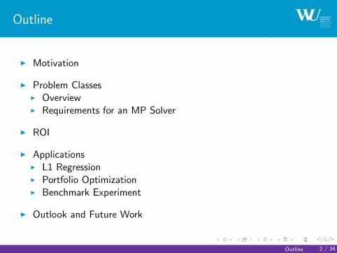
I Motivation
I Problem ClassesI OverviewI Requirements for an MP Solver
I ROI
I ApplicationsI L1 RegressionI Portfolio OptimizationI Benchmark Experiment
I Outlook and Future Work
Outline 2 / 34

. . . . . .
Motivation
Motivation 3 / 34
. . . . . .
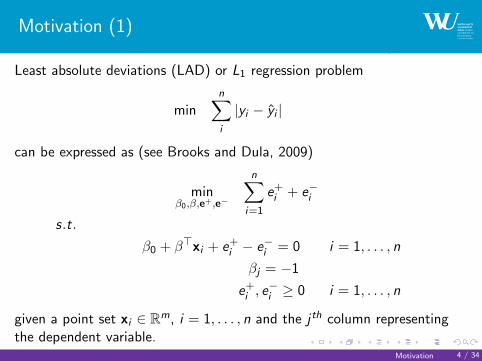
Motivation (1)
Least absolute deviations (LAD) or L1 regression problem
minn∑i
|yi − yi |
can be expressed as (see Brooks and Dula, 2009)
minβ0,β,e+,e−
n∑i=1
e+i + e−i
s.t.
β0 + β>xi + e+i − e−i = 0 i = 1, . . . , n
βj = −1
e+i , e−i ≥ 0 i = 1, . . . , n
given a point set xi ∈ Rm, i = 1, . . . , n and the j th column representingthe dependent variable.
Motivation 4 / 34
. . . . . .
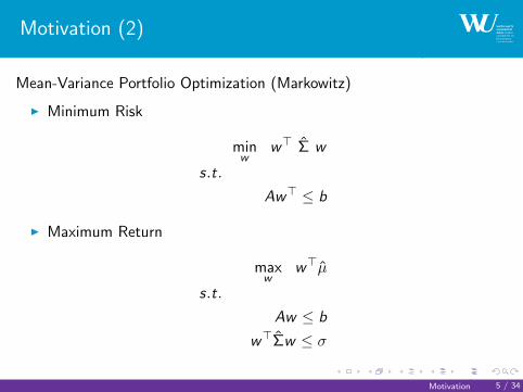
Motivation (2)
Mean-Variance Portfolio Optimization (Markowitz)
I Minimum Risk
minw
w> Σ w
s.t.
Aw> ≤ b
I Maximum Return
maxw
w>µ
s.t.
Aw ≤ b
w>Σw ≤ σ
Motivation 5 / 34

. . . . . .
Problem Classes
Problem Classes 6 / 34
. . . . . .
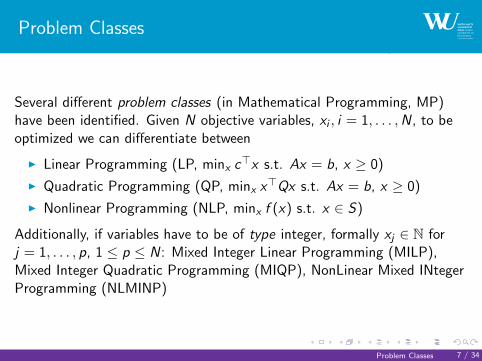
Problem Classes
Several different problem classes (in Mathematical Programming, MP)have been identified. Given N objective variables, xi , i = 1, . . . ,N, to beoptimized we can differentiate between
I Linear Programming (LP, minx c>x s.t. Ax = b, x ≥ 0)
I Quadratic Programming (QP, minx x>Qx s.t. Ax = b, x ≥ 0)
I Nonlinear Programming (NLP, minx f (x) s.t. x ∈ S)
Additionally, if variables have to be of type integer, formally xj ∈ N forj = 1, . . . , p, 1 ≤ p ≤ N: Mixed Integer Linear Programming (MILP),Mixed Integer Quadratic Programming (MIQP), NonLinear Mixed INtegerProgramming (NLMINP)
Problem Classes 7 / 34
. . . . . .
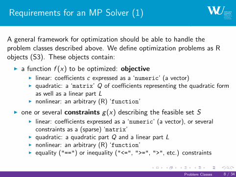
Requirements for an MP Solver (1)
A general framework for optimization should be able to handle theproblem classes described above. We define optimization problems as Robjects (S3). These objects contain:
I a function f (x) to be optimized: objectiveI linear: coefficients c expressed as a ‘numeric’ (a vector)I quadratic: a ‘matrix’ Q of coefficients representing the quadratic form
as well as a linear part LI nonlinear: an arbitrary (R) ‘function’
I one or several constraints g(x) describing the feasible set SI linear: coefficients expressed as a ‘numeric’ (a vector), or several
constraints as a (sparse) ‘matrix’I quadratic: a quadratic part Q and a linear part LI nonlinear: an arbitrary (R) ‘function’I equality ("==") or inequality ("<=", ">=", ">", etc.) constraints
Problem Classes 8 / 34
. . . . . .
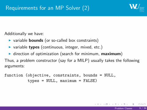
Requirements for an MP Solver (2)
Additionally we have:
I variable bounds (or so-called box constraints)
I variable types (continuous, integer, mixed, etc.)
I direction of optimization (search for minimum, maximum)
Thus, a problem constructor (say for a MILP) usually takes the followingarguments:
function (objective, constraints, bounds = NULL,
types = NULL, maximum = FALSE)
Problem Classes 9 / 34
. . . . . .
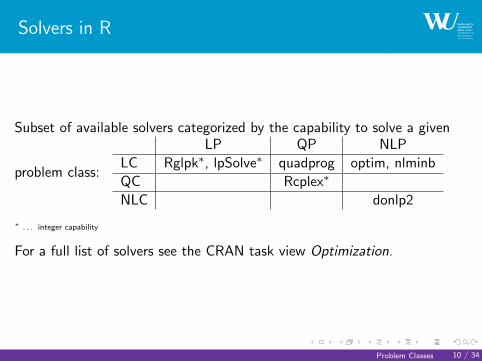
Solvers in R
Subset of available solvers categorized by the capability to solve a given
problem class:
LP QP NLP
LC Rglpk∗, lpSolve∗ quadprog optim, nlminb
QC Rcplex∗
NLC donlp2
∗ . . . integer capability
For a full list of solvers see the CRAN task view Optimization.
Problem Classes 10 / 34
. . . . . .
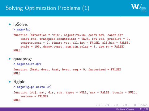
Solving Optimization Problems (1)
I lpSolve:> args(lp)
function (direction = "min", objective.in, const.mat, const.dir,
const.rhs, transpose.constraints = TRUE, int.vec, presolve = 0,
compute.sens = 0, binary.vec, all.int = FALSE, all.bin = FALSE,
scale = 196, dense.const, num.bin.solns = 1, use.rw = FALSE)
NULL
I quadprog:> args(solve.QP)
function (Dmat, dvec, Amat, bvec, meq = 0, factorized = FALSE)
NULL
I Rglpk:> args(Rglpk_solve_LP)
function (obj, mat, dir, rhs, types = NULL, max = FALSE, bounds = NULL,
verbose = FALSE)
NULL
Problem Classes 11 / 34
. . . . . .
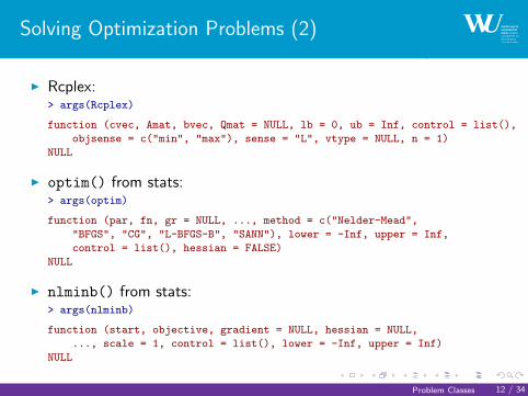
Solving Optimization Problems (2)
I Rcplex:> args(Rcplex)
function (cvec, Amat, bvec, Qmat = NULL, lb = 0, ub = Inf, control = list(),
objsense = c("min", "max"), sense = "L", vtype = NULL, n = 1)
NULL
I optim() from stats:> args(optim)
function (par, fn, gr = NULL, ..., method = c("Nelder-Mead",
"BFGS", "CG", "L-BFGS-B", "SANN"), lower = -Inf, upper = Inf,
control = list(), hessian = FALSE)
NULL
I nlminb() from stats:> args(nlminb)
function (start, objective, gradient = NULL, hessian = NULL,
..., scale = 1, control = list(), lower = -Inf, upper = Inf)
NULL
Problem Classes 12 / 34

. . . . . .
ROI
ROI 13 / 34
. . . . . .
ROI
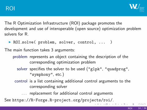
The R Optimization Infrastructure (ROI) package promotes thedevelopment and use of interoperable (open source) optimization problemsolvers for R.
I ROI solve( problem, solver, control, ... )
The main function takes 3 arguments:
problem represents an object containing the description of thecorresponding optimization problem
solver specifies the solver to be used ("glpk", "quadprog","symphony", etc.)
control is a list containing additional control arguments to thecorresponding solver
. . . replacement for additional control arguments
See https://R-Forge.R-project.org/projects/roi/.
ROI 14 / 34
. . . . . .
Examples: ROI and Constraints
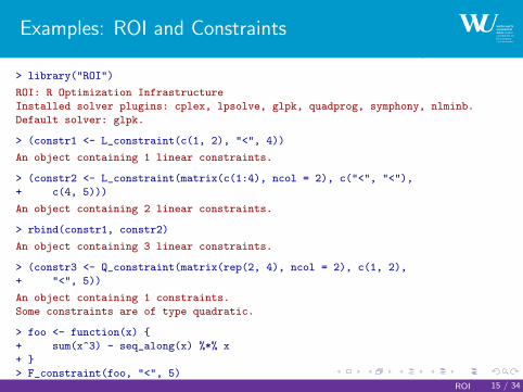
> library("ROI")
ROI: R Optimization Infrastructure
Installed solver plugins: cplex, lpsolve, glpk, quadprog, symphony, nlminb.
Default solver: glpk.
> (constr1 <- L_constraint(c(1, 2), "<", 4))
An object containing 1 linear constraints.
> (constr2 <- L_constraint(matrix(c(1:4), ncol = 2), c("<", "<"),
+ c(4, 5)))
An object containing 2 linear constraints.
> rbind(constr1, constr2)
An object containing 3 linear constraints.
> (constr3 <- Q_constraint(matrix(rep(2, 4), ncol = 2), c(1, 2),
+ "<", 5))
An object containing 1 constraints.
Some constraints are of type quadratic.
> foo <- function(x) {
+ sum(x^3) - seq_along(x) %*% x
+ }
> F_constraint(foo, "<", 5)
An object containing 1 constraints.
Some constraints are of type nonlinear.
ROI 15 / 34
. . . . . .
Examples: Optimization Instances
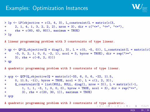
> lp <- LP(objective = c(2, 4, 3), L_constraint(L = matrix(c(3,
+ 2, 1, 4, 1, 3, 2, 2, 2), nrow = 3), dir = c("<=", "<=", "<="),
+ rhs = c(60, 40, 80)), maximum = TRUE)
> lp
A linear programming problem with 3 constraints of type linear.
> qp <- QP(Q_objective(Q = diag(1, 3), L = c(0, -5, 0)), L_constraint(L = matrix(c(-4,
+ -3, 0, 2, 1, 0, 0, -2, 1), ncol = 3, byrow = TRUE), dir = rep(">=",
+ 3), rhs = c(-8, 2, 0)))
> qp
A quadratic programming problem with 3 constraints of type linear.
> qcp <- QCP(Q_objective(Q = matrix(c(-33, 6, 0, 6, -22, 11.5,
+ 0, 11.5, -11), byrow = TRUE, ncol = 3), L = c(1, 2, 3)),
+ Q_constraint(Q = list(NULL, NULL, diag(1, nrow = 3)), L = matrix(c(-1,
+ 1, 1, 1, -3, 1, 0, 0, 0), byrow = TRUE, ncol = 3), dir = rep("<=",
+ 3), rhs = c(20, 30, 1)), maximum = TRUE)
> qcp
A quadratic programming problem with 3 constraints of type quadratic.
ROI 16 / 34
. . . . . .
Examples: Solving LPs
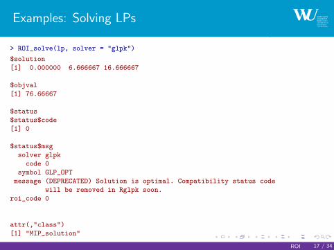
> ROI_solve(lp, solver = "glpk")
$solution
[1] 0.000000 6.666667 16.666667
$objval
[1] 76.66667
$status
$status$code
[1] 0
$status$msg
solver glpk
code 0
symbol GLP_OPT
message (DEPRECATED) Solution is optimal. Compatibility status code
will be removed in Rglpk soon.
roi_code 0
attr(,"class")
[1] "MIP_solution"
ROI 17 / 34
. . . . . .
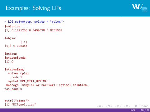
Examples: Solving LPs
> ROI_solve(qcp, solver = "cplex")
$solution
[1] 0.1291236 0.5499528 0.8251539
$objval
[,1]
[1,] 2.002347
$status
$status$code
[1] 0
$status$msg
solver cplex
code 1
symbol CPX_STAT_OPTIMAL
message (Simplex or barrier): optimal solution.
roi_code 0
attr(,"class")
[1] "MIP_solution"
ROI 18 / 34
. . . . . .
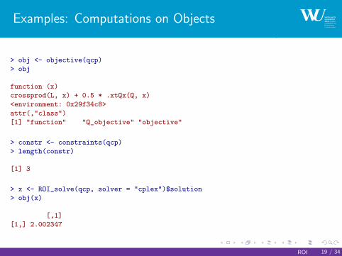
Examples: Computations on Objects
> obj <- objective(qcp)
> obj
function (x)
crossprod(L, x) + 0.5 * .xtQx(Q, x)
<environment: 0x29f34c8>
attr(,"class")
[1] "function" "Q_objective" "objective"
> constr <- constraints(qcp)
> length(constr)
[1] 3
> x <- ROI_solve(qcp, solver = "cplex")$solution
> obj(x)
[,1]
[1,] 2.002347
ROI 19 / 34
. . . . . .
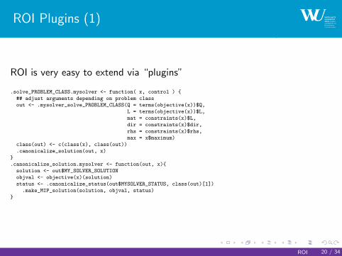
ROI Plugins (1)
ROI is very easy to extend via “plugins”
.solve_PROBLEM_CLASS.mysolver <- function( x, control ) {
## adjust arguments depending on problem class
out <- .mysolver_solve_PROBLEM_CLASS(Q = terms(objective(x))$Q,
L = terms(objective(x))$L,
mat = constraints(x)$L,
dir = constraints(x)$dir,
rhs = constraints(x)$rhs,
max = x$maximum)
class(out) <- c(class(x), class(out))
.canonicalize_solution(out, x)
}
.canonicalize_solution.mysolver <- function(out, x){
solution <- out$MY_SOLVER_SOLUTION
objval <- objective(x)(solution)
status <- .canonicalize_status(out$MYSOLVER_STATUS, class(out)[1])
.make_MIP_solution(solution, objval, status)
}
ROI 20 / 34
. . . . . .
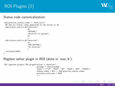
ROI Plugins (2)
Status code canonicalization:
.add_mysolver_status_codes <- function(){
## add all status codes generated by the solver to db
add_status_code_to_db("mysolver",
0L,
"OPTIMAL",
"Solution is optimal",
0L
)
add_status_code_to_db("mysolver",
1L,
"NOT_OPTIMAL",
"No solution."
)
invisible(TRUE)
}
Register solver plugin in ROI (done in ‘zzz.R’):
ROI_register_plugin( ROI_plugin(solver = "mysolver",
package = "mysolverpkg",
types = c("LP", "MILP", "QP", "MIQP", "QCP", "MIQCP"),
status_codes = ROI:::.add_mysolver_status_codes,
multiple_solutions = TRUE
) )
ROI 21 / 34
. . . . . .
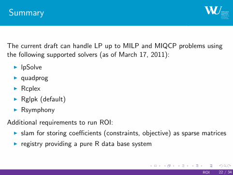
Summary
The current draft can handle LP up to MILP and MIQCP problems usingthe following supported solvers (as of March 17, 2011):
I lpSolve
I quadprog
I Rcplex
I Rglpk (default)
I Rsymphony
Additional requirements to run ROI:
I slam for storing coefficients (constraints, objective) as sparse matrices
I registry providing a pure R data base system
ROI 22 / 34

. . . . . .
Applications
Applications 23 / 34
. . . . . .
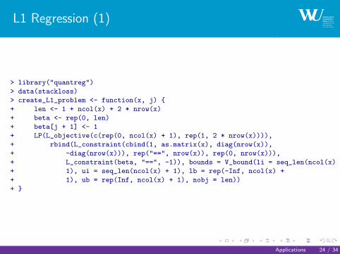
L1 Regression (1)
> library("quantreg")
> data(stackloss)
> create_L1_problem <- function(x, j) {
+ len <- 1 + ncol(x) + 2 * nrow(x)
+ beta <- rep(0, len)
+ beta[j + 1] <- 1
+ LP(L_objective(c(rep(0, ncol(x) + 1), rep(1, 2 * nrow(x)))),
+ rbind(L_constraint(cbind(1, as.matrix(x), diag(nrow(x)),
+ -diag(nrow(x))), rep("==", nrow(x)), rep(0, nrow(x))),
+ L_constraint(beta, "==", -1)), bounds = V_bound(li = seq_len(ncol(x) +
+ 1), ui = seq_len(ncol(x) + 1), lb = rep(-Inf, ncol(x) +
+ 1), ub = rep(Inf, ncol(x) + 1), nobj = len))
+ }
Applications 24 / 34
. . . . . .
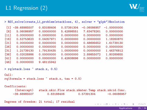
L1 Regression (2)
> ROI_solve(create_L1_problem(stackloss, 4), solver = "glpk")$solution
[1] -39.68985507 0.83188406 0.57391304 -0.06086957 -1.00000000
[6] 5.06086957 0.00000000 5.42898551 7.63478261 0.00000000
[11] 0.00000000 0.00000000 0.00000000 0.00000000 0.00000000
[16] 0.52753623 0.04057971 0.00000000 0.00000000 1.18260870
[21] 0.00000000 0.00000000 0.00000000 0.48695652 1.61739130
[26] 0.00000000 0.00000000 0.00000000 0.00000000 0.00000000
[31] 1.21739130 1.79130435 1.00000000 0.00000000 1.46376812
[36] 0.02028986 0.00000000 0.00000000 2.89855072 1.80289855
[41] 0.00000000 0.00000000 0.42608696 0.00000000 0.00000000
[46] 0.00000000 9.48115942
> rq(stack.loss ~ stack.x, 0.5)
Call:
rq(formula = stack.loss ~ stack.x, tau = 0.5)
Coefficients:
(Intercept) stack.xAir.Flow stack.xWater.Temp stack.xAcid.Conc.
-39.68985507 0.83188406 0.57391304 -0.06086957
Degrees of freedom: 21 total; 17 residual
Applications 25 / 34
. . . . . .
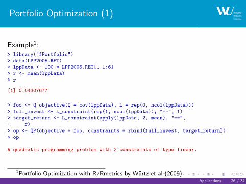
Portfolio Optimization (1)
Example1:> library("fPortfolio")
> data(LPP2005.RET)
> lppData <- 100 * LPP2005.RET[, 1:6]
> r <- mean(lppData)
> r
[1] 0.04307677
> foo <- Q_objective(Q = cov(lppData), L = rep(0, ncol(lppData)))
> full_invest <- L_constraint(rep(1, ncol(lppData)), "==", 1)
> target_return <- L_constraint(apply(lppData, 2, mean), "==",
+ r)
> op <- QP(objective = foo, constraints = rbind(full_invest, target_return))
> op
A quadratic programming problem with 2 constraints of type linear.
1Portfolio Optimization with R/Rmetrics by Wurtz et al (2009)Applications 26 / 34
. . . . . .
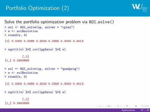
Portfolio Optimization (2)
Solve the portfolio optimization problem via ROI solve()> sol <- ROI_solve(op, solver = "cplex")
> w <- sol$solution
> round(w, 4)
[1] 0.0000 0.0086 0.2543 0.3358 0.0000 0.4013
> sqrt(t(w) %*% cov(lppData) %*% w)
[,1]
[1,] 0.2450869
> sol <- ROI_solve(op, solver = "quadprog")
> w <- sol$solution
> round(w, 4)
[1] 0.0000 0.0086 0.2543 0.3358 0.0000 0.4013
> sqrt(t(w) %*% cov(lppData) %*% w)
[,1]
[1,] 0.2450869
Applications 27 / 34
. . . . . .
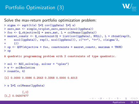
Portfolio Optimization (3)
Solve the max-return portfolio optimization problem:> sigma <- sqrt(t(w) %*% cov(lppData) %*% w)
> zero_mat <- simple_triplet_zero_matrix(ncol(lppData))
> foo <- Q_objective(Q = zero_mat, L = colMeans(lppData))
> maxret_constr <- Q_constraint(Q = list(cov(lppData), NULL), L = rbind(rep(0,
+ ncol(lppData)), rep(1, ncol(lppData))), c("<=", "<="), c(sigma^2,
+ 1))
> op <- QCP(objective = foo, constraints = maxret_constr, maximum = TRUE)
> op
A quadratic programming problem with 2 constraints of type quadratic.
> sol <- ROI_solve(op, solver = "cplex")
> w <- sol$solution
> round(w, 4)
[1] 0.0000 0.0086 0.2543 0.3358 0.0000 0.4013
> w %*% colMeans(lppData)
[,1]
[1,] 0.04307677
Applications 28 / 34
. . . . . .
Benchmark Experiment
Applications 29 / 34
. . . . . .
MIPLIB2003
I A collection of real-world mixed integer programs.
I Standard test set used to compare the performance of MILP solvers.
I Available online at http://miplib.zib.de/miplib2003.php.
I Maintained by Alexander Martin, Tobias Achterberg and ThorstenKoch.
I Instances in MPS file format which can be read via Rglpk’s MPS filereader.
I We can easily run those examples using different solvers via ROI.
Applications 30 / 34
. . . . . .
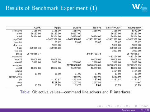
Results of Benchmark Experiment (1)
GLPK Rglpk lp solve lpSolve SYMPHONY Rsymphonyaflow30a 1158.00 1158.00 1158.00 1158.00 1158.00 1159.00
air04 56137.00 56137.00 56137.00 56137.00 56137.00air05 26374.00 26374.00 26374.00 26374.00 26374.00 26374.00
cap6000 −2451377.00 −2451380.00 −2451377.00 −2451377.00 −2451377.00danoint 65.67 65.67 65.67 65.67 65.67disctom −5000.00 −5000.00 −5000.00
fiber 405935.18 405935.18 405935.18 405935.18fixnet6 3983.00 3983.00gesa2 25779856.37 24534703.78 25779856.37
manna81 −13164.00 −13164.00mas76 40005.05 40005.05 40005.05 40005.05 40005.05misc07 2810.00 2810.00 2810.00 2810.00 2810.00 2810.00
modglob 20740500.00 20740508.09 20740508.09 20740508.09nw04 16862.00 16862.00 16862.00 16862.00 16862.00 16862.00p2756 3124.00 3124.00
pk1 11.00 11.00 11.00 11.00 11.00 11.00pp08aCUTS 7350.00 7380.00 7350.00 7350.00
qiu −132.87 −132.87 −32.06 −132.87 −132.87rout 1127.54 1077.56 1077.56 −Inf
vpm2 13.75 13.75 13.75 7.00 13.75 13.75
Table: Objective values—command line solvers and R interfaces
Applications 31 / 34
. . . . . .
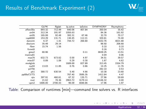
Results of Benchmark Experiment (2)
GLPK Rglpk lp solve lpSolve SYMPHONY Rsymphonyaflow30a 893.32 712.49 640.06 407.84 350.04 35.42
air04 312.34 191.97 1055.63 84.36 161.92air05 165.08 92.48 393.31 67.46 32.70 70.17
cap6000 153.29 131.71 130.45 112.21 320.81 74.40danoint 6.37 1.41 744.72 268.80 1632.76 4021.88disctom 35.49 29.14 98.50 206.68
fiber 15.74 1.56 0.10 0.10fixnet6 0.16 0.73gesa2 80.96 0.11 8639.25 13.51
manna81 0.04 0.06mas76 632.73 673.62 0.00 4.97 34.51 39.57misc07 0.89 1.06 0.29 0.30 1.67 4.62
modglob 1689.69 827.89 313.45 1554.79nw04 13.03 11.85 0.76 0.86 14.25 11.76p2756 282.10 0.53
pk1 380.72 630.54 5.48 4.66 10.38 23.60pp08aCUTS 767.40 3595.35 1412.84 4.47
qiu 397.91 460.61 67.32 135.71 27.96 59.69rout 21.62 78.36 2963.72 3179.14 10146.32 0.00
vpm2 1686.00 2706.43 96.09 4048.86 17.96 1.97
Table: Comparison of runtimes [min]—command line solvers vs. R interfaces
Applications 32 / 34
. . . . . .
Outlook and Future Work
I Optimization terminology (What is a solution?)
I Status codes (What is a reasonable set of status codes?)
I NLP solvers (optim(), nlminb(), Rsolnp, etc.)
I Interfaces to NLMINP solvers Bonmin and LaGO (project RINO onR-Forge)
I Parallel computing and optimizers (e.g., SYMPHONY’s or CPLEX’parallel solver)
I Applications (e.g., fPortfolio, relations, etc.)
Outlook and Future Work 33 / 34

. . . . . .
Thank you for your attention
Stefan TheußlDepartment of Finance, Accounting and StatisticsInstitute for Statistics and Mathematicsemail: [email protected]: http://statmath.wu.ac.at/~theussl
WU Wirtschaftsuniversitat WienAugasse 2–6, A-1090 Wien
Outlook and Future Work 34 / 34