Embed Size (px)
Citation preview

Systematic Review of Bankruptcy Prediction Models: Towards A Framework for Tool Selection
Hafiz A. Alaka1, Lukumon O. Oyedele2, Hakeem A. Owolabi 3, Vikas Kumar 4, Saheed O. Ajayi5, and Olugbenga O. Akinade6, Muhammad Bilal7
1 Senior Lecturer, Faculty of Engineering, Environment and Computing, Coventry University, Coventry, United Kingdom. [email protected]
2 Professor, Bristol Enterprise Research and Innovation Centre (BERIC), University of the West of England, Bristol, United Kingdom. [email protected]
3 Lecturer, Department of International Strategy & Business, The University of Northampton, United Kingdom. [email protected]
4 Professor, Bristol Enterprise Research and Innovation Centre (BERIC), University of the West of England, Bristol, United Kingdom. [email protected]
5 Senior Lecturer, School of Built Environment and Engineering, Leeds Becket University, Leeds, United Kingdom. [email protected]
6 Research Fellow, Bristol Enterprise Research and Innovation Centre (BERIC), University of the West of England, Bristol, United Kingdom. [email protected]
7 Research Fellow, Bristol Enterprise Research and Innovation Centre (BERIC), University of the West of England, Bristol, United Kingdom. [email protected]
1

Abstract
The bankruptcy prediction research domain continues to evolve with many new different predictive models
developed using various tools. Yet many of the tools are used with the wrong data conditions or for the wrong
situation. Using the Web of Science, Business Source Complete and Engineering Village databases, a
systematic review of 49 journal articles published between 2010 and 2015 was carried out. This review shows
how eight popular and promising tools perform based on 13 key criteria within the bankruptcy prediction models
research area. These tools include two statistical tools: multiple discriminant analysis and Logistic regression;
and six artificial intelligence tools: artificial neural network, support vector machines, rough sets, case based
reasoning, decision tree and genetic algorithm. The 13 criteria identified include accuracy, result transparency,
fully deterministic output, data size capability, data dispersion, variable selection method required, variable types
applicable, and more. Overall, it was found that no single tool is predominantly better than other tools in relation
to the 13 identified criteria. A tabular and a diagrammatic framework are provided as guidelines for the selection
of tools that best fit different situations. It is concluded that an overall better performance model can only be
found by informed integration of tools to form a hybrid model. This paper contributes towards a thorough
understanding of the features of the tools used to develop bankruptcy prediction models and their related
shortcomings.
Keywords: Bankruptcy prediction tools; Financial ratios; Error types; systematic review; tool selection framework; artificial intelligence tools, statistical tools.
2

1.0 Introduction
The effect of high rate of business failure can be devastating to firm owner, partners, society and the country’s
economy at large (Edum-Fotwe et al., 1996; Xu and Zhang, 2009; Hafiz et al., 2015; Alaka et al., 2015). The
consequent extensive research into developing bankruptcy prediction models (BPM) for firms is undoubtedly
justified. The performance of such models is largely dependent on, among other factors, the choice of tool
selected to build it. Apart from a few studies (e.g. Altman, 1968; Ohlson, 1980), tool selection in many BPM
studies is not based on capabilities of the tool; rather it is either chosen based on popularity (e.g. Langford et al.,
1993; Abidali and Harris, 1995; Koyuncugil and Ozgulbas, 2012) or based on professional background (e.g.
Altman et al., 1994; Nasir et al., 2000; Lin and Mcclean, 2001; Hillegeist et al., 2004; Beaver et al., 2005). This
is because there is no evaluation material which shows and compares the relative performance of major tools in
relation to the many important criteria a BPM should satisfy. Such material can provide a guideline and
subsequently aid an informed and justified tool selection for BPM developers.
Most prediction tools are either statistical or artificial intelligence (AI) based (Jo and Han, 1996; Balcaen and
Ooghe, 2006). The most common statistical tool is the multiple discriminant analysis (MDA) which was first
used by Altman (1968) to develop a BPM popularly known as Z model, based on Beaver’s (1966)
recommendation in his univariate work. MDA, normally used with financial ratios (quantitative variables),
subsequently became popular with accounting and finance literature (Taffler, 1982) and many subsequent
studies by finance professionals simply adopted MDA without considering the assumptions that are to be
satisfied for MDA’s model to be valid. This resulted in inappropriate application, causing developed models to
be un-generalizable (Joy and Tollefson, 1975; Richardson and Davidson, 1984; Zavgren, 1985). Abidali and
Harris (1995), for example, unscholarly employed A-score alongside Z-score (i.e. MDA) in order to involve
qualitative managerial variables, alongside quantitative variables, in their analysis when logistic regression (LR)
[or logit analysis] can handle both types of variables singularly.
AI tools are computer based techniques of which Artificial Neural Network (ANN or NN) is the most common
for bankruptcy prediction (Aziz and Dar, 2006; Tseng and Hu, 2010). Simply because it is the most popular
architecture, many studies arbitrarily employed the back-propagation algorithm of ANN for bankruptcy
prediction (e.g. Odom and Sharda, 1990; Tam and Kiang, 1992; Wilson and Sharda, 1994; Boritz et al., 1995;
among others) despite it having a number of relatively undesirable features which include computational
intensity, absence of formal theory, “illogical network behaviour in response to different variations of the input
values” etc. (Coats and Fant, 1993; Altman et al., 1994, p. 507; Zhang et al., 1999). Further, Fletcher and Goss
(1993) developed an ANN prediction model for a relatively small sample size when ANNs are known to need
large samples for optimal performance (Boritz et al., 1995; Shin et al., 2005; Ravi Kumar and Ravi, 2007).
These improper uses of tools regularly occur because there is no readily available evaluation material or
guidelines which can help BPM developers identify which tool best suits what data/purpose/situation. As Chung
3

et al. (2008, p. 20) put it, “given the variety of techniques now available for insolvency prediction, it is not only
necessary to understand the uses and strengths of any prediction model, but to understand their limitations as
well”. Hence to ensure a BPM performs well with regards to criteria of preference (e.g. accuracy, type I error,
transparency, among others), a model developer has to understand the strength and limitations of the available
tools/techniques. This will ensure that the right tool is employed for the right data characteristics, right situation
and the right purpose. This study thus aims to develop a comprehensive evaluation framework for selection of
BPM tools using a systematic and comprehensive review. The following objectives are needed to achieve this
aim:
1. Presentation of an overview of the common tools used for bankruptcy prediction and identification of BPM studies that have used these tools
2. Identifying the key criteria BPMs need to satisfy and how each tool performs in relation to each criterion by analysing the systematic review
The scope of this study is limited to reviewing only popular and promising tools that have been employed for the
development of BPMs in past studies since interest in them is high. This is because it is virtually impossible to
review all the many tools that can be used for this purpose in this study. In total, two statistical and six AI tools
were reviewed. The next section explains the systematic review methodology used in this study with all the
inclusion and exclusion criteria. This is followed by a brief description of each of the eight tools. Section four
presents the 13 identified key criteria used to assess the tools. Section five discusses the analysis and results of
the review in form of tables and charts. Section six presents the proposed tabular and diagrammatic frameworks.
This is followed up with a conclusion section.
2.0 Methodology
This study used a systematic review method to create a guideline for the selection of an appropriate tool for
developing a bankruptcy prediction model (BPM). There are so many tools that can be used to develop a BPM
that it is virtually impossible to review them all in one study. As a result, the two most popular statistical tools as
noted by Balcaen and Ooghe (2006) in their comprehensive review of BPMs were reviewed: multiple
discriminant analysis (MDA) and Logistic regression (LR). Also covered in this review are the most popular
and promising artificial intelligence (AI) tools as advocated by Aziz and Dar (2006) in their comprehensive
review, and Min et al. (2006) among others: artificial neural network (ANN), support vector machines (SVM),
rough sets (RS), case based reasoning (CBR), decision tree (DT) and genetic algorithm (GA). A process flow of
the methodology is presented in Figure 1.
Systematic review is a well-known method for producing valid and reliable knowledge as it minimizes bias
hence its popularity in the all-important medical research world (Tranfield et al., 2003; Schlosser, 2007). The
inclusion criteria for this study were carefully chosen to allow fair comparison and ensure adequate quality
4

(Khan et al., 2003). To improve validity of this study, only peer reviewed journal articles were considered since
they are considered to be of high quality and their contribution considered as very valid (Schlosser, 2007).
Figure 1: Process flow of the methodology (the term ‘considered tool’ refers to the eight tools considered in this study).
Systematic review requires wide literature search (Smith et al., 2011) hence following Appiah et al. (2015)
approach, which is the most recently published systematic review in the BPM research area, the following
5

databases were considered: Google Scholar; Wiley Interscience; Science Direct; Web of Science UK (WoS); and
Business Source Complete (BSC). However, a careful observation revealed Google scholar produced an almost
endless result and did not have the required filters to make it very efficient hence it was removed as it was
unmanageable. Further observation revealed that (WoS) and BSC contained all the journal articles provided in
Wiley and Science Direct; this is probably because the latter two are publishers while the former two are
databases with articles from various publishers including the latter two. To increase the width of the search,
Engineering Village (EV) database was added to WoS and BSC databases to perform the final search. EV was
chosen because articles from the engineering world usually deal with BPM tools comprehensively.
The initial searches in the three databases (WoS, BSC and EV) showed that studies tend to use bankruptcy,
insolvency and financial distress as synonyms for failure of firms. A search framework which captured all these
words was thus designed with the following defined string (“Forecasting” OR “Prediction” OR “Predicting”)
AND (“Bankruptcy” OR “Insolvency” OR “Distress” OR “Default” OR “Failure”).
To ensure high consistency and repeatability of this study, and consequently reliability and quality (Stenbacka,
2001; Trochim and Donnelly, 2006), only studies that appeared in the three databases were used; this ensured the
eradication of database bias (Schlosser, 2007). These databases contain studies from all over the world hence
geographic bias was also eliminated. Balcaen and Ooghe (2006) in their comprehensive review of statistical
tools in 2006 noted that AI tools, mainly ANN, were gradually becoming adopted in BPM studies. With new
tools emerging all the time, a four-year advance from 2006, which would have seen more use of AI tools, is how
a start year of 2010 was chosen for this study. The end year is the year this paper was written, 2015.
Generally, the topic of articles that emerge from the search looked okay to determine which ones were fit for this
study. However, this was not the case for all articles. Where otherwise, article’s abstract was read and, if
necessary, introduction and/or conclusion were read. In some cases, the complete articles had to be read.
Although language constraint is not encouraged in systematic review, it is sometimes unavoidable due to lack of
funds to pay for interpretation services (Smith et al., 2011) as in the case of this study. Only studies written in
English were thus used.
After eliminating unrelated studies that dealt with topics like credit scoring (e.g. Martens et al., 2010), policy
forecasting (e.g. Won et al., 2012), or that did not use any of the tools reviewed (e.g. Martin et al., 2011), only
51 studies had a presence in the three data bases. Of these, two had great ambiguity in reporting their results
hence were excluded, leaving 49 studies to be used as the sample. The ‘review studies’ in the search results (e.g.
Sun et al., 2014) were not considered since original results from tools implementation were needed.
In the final 49 studies sample (i.e. the primary studies used for this systematic review), where results of tools in
their hybrid forms and the result of the tools in their standalone form were presented, results of the tools in their
standalone form was used to allow fair comparisons of inter-study results. However, where any of the eight tools
6

in consideration is used for variable selection and in turn used to hybridise the predicting tool, the result of such
hybrid is used. Where the tools were used on more than one dataset and the results of each dataset was presented
alongside the total average from all dataset, the total average results were used. In cases where average values
were not given, the result set with the best accuracy for most/all of the tools in consideration in this study was
used so as to give all tools a good chance of high accuracy. In cases where the results of more than a year of
prediction were given, the results of the first year were used to allow for fair comparison since most BPM
studies normally present first year results.
As required for systematic review, a meta-analysis was done with data synthesised using ‘summary of findings’
tables, statistical methods and charts (Khan et al., 2003; Higgins, 2008; Smith et al., 2011); with facts explained
sometimes by employing quotes from especially the reviewed studies, and discussions backed up with a wider
review of literature. Three summary of findings tables were provided in this study. Where there is not enough
information from the reviewed studies regarding a certain criterion, results are discussed using the reviewed
studies and wider literature. Opinions are only taken as facts in such cases if there are no opposing studies. This
type of deviation from protocol for a valid reason is acceptable in systematic review (Schlosser, 2007). Finally,
this review is used to create a guideline using a tabular framework for tool comparisons and a diagrammatic
framework that clearly shows what situations/data characteristics/variable types etc. each discussed tool is best
suited to. This will ensure developers can choose a tool based on what they have and/or intend to get rather than
just arbitrarily.
3.0 The Tools
This study will review eight tools used to develop bankruptcy prediction models including: multiple discriminant
analysis (MDA), Logistic regression (LR), artificial neural network (ANN), support vector machines (SVM),
rough sets (RS), case based reasoning (CBR), decision tree (DT) and genetic algorithm (GA).
Multiple Discriminant Analysis: MDA uses a linear combo of variables, normally financial ratios, that best
differentiate between failing and surviving firms to classify firms into one of the two groups. The MDA
function, constructed usually after variable selection, is as follows:
Z = c1X1 + c2X2 + …………… + cnXn.
Where c1, c2, ………. cn, = discriminant coefficients; and X1, X2, …….. Xn = independent variables
MDA calculates the discriminant coefficients. The function is used to calculate a Z-score. A cut-off Z score is
chosen based on status of sample firms
Logistic regression: LR is a “conditional probability model which uses the non-linear maximum log-likelihood
technique to estimate the probability of firm failure under the assumption of a logistic distribution” (Jackson and
Wood, 2013, p. 190). The LR function, constructed after variable selection, is as follows:
7

P1(Vi) = 1/[1 + exp - (b0 + b1Vi1 + b2Vi2 +…...+ bnVin)] = 1/[1 + exp - (Di)]
where P1(Vi) = probability of failure given the vector of attributes; Vi; Vij = value of attribute or variable j (j =
1, 2, ….., n) for firm i; bj = coefficient for attribute j; b0 = intercept; Di = logit of firm i.
The dependent variable P1 is expressed in binary form (0,1) (Boritz and Kennedy, 1995).
Neural Network: ANN was created to imitate how the neural system of the human brain works (Hertz et al.,
1991) and was first applied to bankruptcy prediction by Odom and Sharda (1990). A typical ANN is a network
of nodes interconnected in layers. There are various parameters, architectures, algorithms, and training methods
that can be used to develop an ANN (Jo and Han, 1996) and choosing the best combination can be demanding.
Support vector machines: SVM employs a linear model to develop an optimal separating hyperplane by using
a highly non-linear mapping of input vectors into a high-dimensional feature space (Shin et al., 2005; Ravi
Kumar and Ravi, 2007). It constructs the boundary using binary class. The variables closest to the hyperplane
are called support vectors and are used to define the binary outcome (failing or non-failing) of assessed firms.
All other samples are ignored and are not involved in deciding the binary class boundaries (Vapnik, 1998). Like
ANN, it has some parameters that can be varied for it to perform optimally (Dreiseitl and Ohno-Machado 2002).
Rough Sets: RS theory, discovered by Pawlak (1982), assumes that there is some information associated with
all objects (firms) of a given universe; information which is given by some attributes (variables) that can
describe the objects. Objects that possess the same attributes are indiscernible (similar) with respect to the
chosen attributes. RS creates a partition in the universe that separates objects with similar attributes into blocks
(e.g. failing and non-failing blocks) called elementary sets (Greco et al., 2001). Objects that fall on the boundary
line cannot be classified because information about them is ambiguous. RS is used to extract the decision rules to
solve classification problems (Ravi Kumar and Ravi, 2007; Greco et al., 2001).
Case Based Reasoning: CBR fundamentally differs from other tools in that it does not try to recognize pattern,
rather it classifies a firm based on a sample firm that possess similar attribute values (Shin and Lee, 2002). It
justifies its decision by presenting the used sample cases (firms) from its case library (Kolodner, 1993). It
induces decision rules for classification.
Decision Tree: DT became an important machine learning tool after Quinlan (1986) developed iterative
dichotomiser 3 (ID3). DT uses entropy to measure the discriminant power of samples’ variables and
subsequently recursively partitions (RPA) the set of data for the classification of firms (Quinlan, 1986). Quinlan
(1993) later developed the advanced version called Classifier 4.5 (C4.5). DT induces the decision rules. The
positions of the rules in the decision tree are usually determined using heuristics (Jeng et al., 1997). For example,
if profitability was found to be more important than liquidity, it will be placed above, or evaluated before,
liquidity.
8

Genetic Algorithm: GA is a searching optimization technique that imitates the Darwin principle of evolution in
solving nonlinear, non-convex problems (Ravi Kumar and Ravi, 2007). It is effective at locating the global
minimum in a very large space. It differs from other tools in that it simultaneously searches multiple points,
works with character springs and uses probabilistic and not deterministic rules. GA can extract decision rules
from data which can be used for classifying firms. It is applied to selected variables in order to find a cut-off
score for each variable (Shin and Lee, 2002).
4.0 Important Criteria Required for Bankruptcy Prediction Model Tools
To be considered effective, there are many criteria that can be required to be satisfied by a tool when it is used to
develop a bankruptcy prediction model (BPM). The set of criteria required usually depend on the situation and
intention of the BPM developer. For example, a financier or client may simply be interested in the accuracy of a
model. The BPM needed simply needs to be able to predict if a firm is financially healthy (unhealthy) enough to
be granted (refused) a loan or contract, hence a highly accurate tool/technique is needed. A firm owner on the
other hand is interested in result transparency as much as accuracy because he needs to know where/what the
firm is going/doing wrong in order to know where rescue efforts need to be focused on. In such a case, a tool
with high accuracy as well as result transparency will be needed to build the required BPM
Different researchers have used different criteria to develop their BPMs, however after a thorough and
comprehensive review of the primary studies and other studies in the area, 13 criteria were identified to be the
most common and important. Example of other reviewed studies include Tam and Kiang, (1992); Haykin,
(1994); Zurada et al., (1994); Edum-Fotwe et al., (1996); Dreiseitl and Ohno-Machado, (2002); Min and Lee,
(2005); Shin et al., (2005); Balcaen and Ooghe, (2006); Ravi Kumar and Ravi, (2007); Chung et al., (2008); Ahn
and Kim, (2009); to mention a few. The identified 13 criteria are as follows:
1) Accuracy: This relates to the percentage of firms a tool correctly classifies as failing or non-failing.
2) Result transparency: This has to do with interpretability of a tool’s result.
3) Non-deterministic: The case where a tool cannot successfully classify a firm
4) Sample size: This refers to the sample size(s) suitable for a tool to perform optimally.
5) Data dispersion: This refers to ability of a tool to handle equally or unequally dispersed data
6) Variable selection: This refers to the variables selection methods required for optimum tool performance.
7) Multicollinearity: This refers to sensitivity of a tool to collinear variables.
8) Variable types: A tool’s capability to analyse quantitative and/or qualitative variables.
9) Variable relationship: This explains a tool’s limitation in analysing linear or non-linear variables
10) Assumptions imposed by tools: Requirements a sample data has to satisfy for a tool to perform optimally.
9

11) Sample specificity/overfitting: This is when the model developed from a tool performs well on sample firms
but badly on validation data.
12) Updatability: The ease with which a tool’s model can be updated with new sample firms and its
effectiveness afterwards
13) Integration capability: the ease with which a tool is hybridisable.
These 13 criteria can be grouped into three main categories as shown in Figure 2. These categories are:
1) Results related criteria
2) Data related criteria
3) Tool’s properties related criteria
Figure 2: Important criteria required for BPM tools
5.0 Results and Discussion
This section presents the results, analysis and discussion of the systematic review in form of summary of
findings tables and statistical charts. The results are presented in relation to each identified criterion. The tables
and charts compare the performance/ability of the tools as deduced from all the reviewed studies. The outcome
is used to judge each tool based on the criterion in question. The criteria were assessed and discussed in the
context of bankruptcy prediction models (BPM). For example, to assess the accuracy criteria of the tools, error
cost had to be considered since it is an important aspect of accuracy assessment in the BPM research area.
Not all the reviewed studies provided necessary tool information required to assess a tool under each criterion.
Where a tool had too few studies providing information regarding a criterion, the tool was excluded from the
10

statistical analysis regarding that criterion. The measure for exclusion was determined by calculating the average
number of studies that provided information on the tools regarding the criterion in consideration; the tools with
numbers well below average were excluded. This process, where employed, is clearly explained.
5.1 Results Related Criteria
5.1.1 Accuracy
One of the main essences of using varying tools to develop BPMs is to increase accuracy of prediction. Figure 3
shows the mean average accuracy chart for each tool calculated from all the studies that gave an accuracy
reading for the tool. The chart includes only the tools that had up to 17 studies that reported an accuracy value
for them since the mean average of number of studies that reported accuracy value is 17 (Table 1). The chart
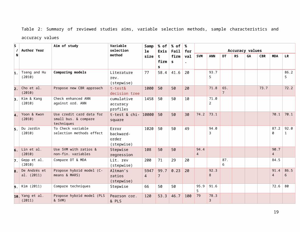
clearly shows ANN and SVM to be the most accurate while MDA appears to be the least accurate. Table 2 is the
first summary of findings table. It shows the accuracy value of each tool as reported in each study.
SVM NN DT MDA LR70.00
72.00
74.00
76.00
78.00
80.00
82.00
84.00
86.00
Avg.
of
accu
racy
val
ues
Figure 3: Overall average accuracy chart for each tool
Table 1: Summary statistics of the accuracy and error types of the tools
Tool No. of authors that used tool
No. of authors that reported an accuracy value
No. of authors that reported Type I error
No. of authors that reported Type II error
SVM 24 22 10 11ANN 38 37 18 18DT 19 17 5 6RS 4 4 1 1GA 10 6 4 4CBR 4 3 0 0MDA 21 19 7 7LR 31 28 12 12Total Fu =151 fac = 136 fo=57 ft=59Mean ∑ fac/∑f = 17 ∑ fo/∑f = 7.1 ∑ ft/∑f = 7.35
11
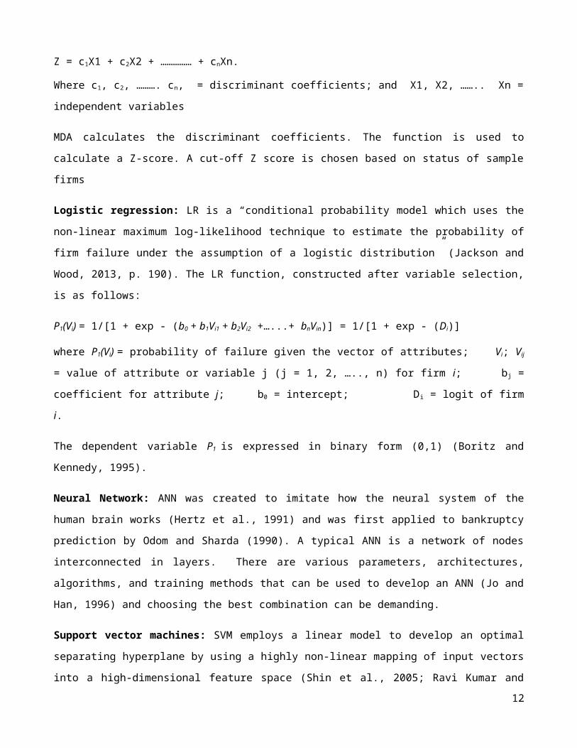
Table 2: Summary of reviewed studies aims, variable selection methods, sample characteristics and accuracy valuesS/
N Author YearAim of study Variable selection
methodSample size
% of Exist firms
% of Fail firms
% for val.
Accuracy valuesSVM ANN DT RS GA CBR MDA LR
1. Tseng and Hu (2010)
Comparing models Literature rev. (stepwise)
77 58.4 41.6 20 93.75 86.25
2. Cho et al. (2010) Propose new CBR approach t-test& decision tree
1000 50 50 20 71.8 65.7 73.7 72.2
3. Kim & Kang (2010) Check enhanced ANN against ord. ANN
cumulative accuracy profiles
1458 50 50 10 71.02
4. Yoon & Kwon (2010)
Use credit card data for small bus. & compare techniques
t-test & chi-square 10000 50 50 30 74.2 73.1 70.1 70.1
5. Du Jardin (2010) To Check variable selection methods effect
Error backward-order (stepwise)
1020 50 50 49 94.03 87.20 92.01
6. Lin et al. (2010) Use SVM with ratios & non-fin. variables
Stepwise regression 108 50 50 94.44 90.74
7. Gepp et al. (2010) Compare DT & MDA Lit. rev (stepwise) 200 71 29 20 87.6 84.58. De Andrés et al.
(2011)Propose hybrid model (C-means & MARS)
Altman’s ratios (stepwise)
59474
99.77 0.23 20 92.38 91.44 86.56
9. Kim (2011) Compare techniques Stepwise 66 50 50 95.95 91.6 72.6 8010. Yang et al. (2011) Propose hybrid model (PLS & SVM) Pearson cor. & PLS 120 53.3 46.7 100 79 78.3311. Chen (2011) Use PSO with SVM Lit. rev. (stepwise),
GA80 50 50 20
12. Divsalar et al. (2011)
Use GA & NN SFS 150 51.4 48.6 82.5 95 80
13. Du Jardin & Séverin (2011)
Use self-organizing map Error backward-order (stepwise)
2360 50 50 37.3 82.61 81.93 81.14
14. Chen et al. (2011b) Integrate error cost into model 1200 50 50 20 90 90.6 86.715. Chen et al. (2011a) Propose FKNN 240 53.3 46.7 10 76.67 79.58 83.3316. Li et al. (2011) Propose Random subspace LR
(RSBL)Stepwise & t-test 370 50 50 30 88.46 88.26 87.50
17. Divsalar et al. (2012)
sequential featureselectionUse new type of GA called GEP
SFS 136 52.5 47.5 33.3 79.41 91.18 76.47
18. Huang et al. (2012) Propose hybrid KLFDA & MR-SVM 10 86.61 83.67 83.24 77.919. Tsai & Cheng
(2012)Check effect of outlier on BPMs 653 45.3 54.7 10 86.37 86.06 84.69 86.37
20. Shie et al. (2012) Proposed enhanced PSO-SVM Factor analysis & PCA
54 55 44.4 81.82 75.76 77.77 72.73
21. Kristóf & Virág (2012)
504 86.7 13.3 25 88.7 88.8 88.5
22. Jeong et al. (2012). To fine-tune ANN factors GAM 2542 50 50 20 79 81 76 73 73.5 76.48
12

S/N Author Year
Aim of study Variable selection method
Sample size
% of Exist firms
% of Fail firms
% for val.
Accuracy valuesSVM ANN DT RS GA CBR MDA LR
23. Du Jardin & Séverin (2012)
To use Kohonen map to stabilize temporal accuracy
81.3 81.2 81.6
24. De Andrés et al. (2012)
To improve performance of classifiers 122 50 50 19.6 76.03 74.87
25. Zhou et al. (2012) To find the best variables for accuracy
Spearman correlation
50 50 10.8 71.1 67.8 75.6 64.4 54.4
26. Xiong et al. (2013) Use sequence on credit card data 70.9427. Lee & Choi (2013) To do multi industry investigation t-test &correlation
analysis1775 66.2 33.8 4.2 92 82.01
28. Tsai & Hsu (2013) Present met-learning framework (hybrid)
MC Avg. many
20 78.82 77.29 79.11
29. Callejón et al (2013) To increase predictive power of ANN 1000 50 50 20 92.1130. Chuang (2013) To Hybridise CBR Multiple 321 86.9 13.1 90.131. Ho et al. (2013) Develop BPM for US paper
companiesLit rev (stepwise) 366 66.7 33.3 20 93
32. Arieshanti et al. (2013)
To compare techniques Lit rev. (stepwise) 240 53.3 46.7 20 70.42 71
33. Kasgari et al. (2013) Compare ANN to other techniques Garson’s algorithm 135 52.5 47.5 25 94.11 88.57 91.4334. Zhou et al. (2014) Propose new feature selection method GA 2010 50 50 75.6 50.67 71.72 73.9935. Tsai (2014) To compare hybrids SOM 690 44.5 55.5 20 91.61 86.83 87.2836. Yeh et al. (2014) To increase accuracy using RF&RS RF 220 75 25 33 94.58 92.95 91.55 96.9937. Wang et al. (2014) Inject feature selection into boosting 132 50 50 10 79.99 75.69 75.99 73.9038. Abellán & Mantas
(2014)To correctly use bagging scheme Lit. rev. (stepwise) 690 30 93.64
39. Tserng et al. (2014) To use LR to predict contractors default
87 66.7 33.3 79.18
40. Yu et al. (2014) Produce BPM using ELM 500 50 50 33.3 93.2 86.541. Gordini (2014) Test GA accuracy & compare to other
techniquesVIF & stepwise 3100 51.6 48.4 30 69.5 71.5 66.8
42. Heo & Yang (2014) To prove AdaBoost is right for Korean construction firms
2762 50 50 20 73.3 77.1 73.1 51.3
43. Tsai et al. (2014) To compare classifier ensembles 690 44.5 55.5 10 86.37 84.38 86.3744. Virág & Nyitrai
(2014)To show RS accuracy is competitive with SVM & ANN
156 50 50 25 89.32 88.03 89.32
45. Liang et al. (2015) To compare feature selections GA 688 50 50 10 91.77 91.63 92.9846. Iturria1 & Sanz
(2015)To develop ANN BPM for US banks Mann-Whintney
test & Gini index772 50 50 13.5 89.42 93.27 77.88 81.73
47. Du Jardin (2015) To improve BPM accuracy beyond one year
16880 50 50 50 80.8 80.1 80.6
48. Bemš et al. (2015). Introduce new scoring method called Gini index
Gini index 459 67 33 579 0.291 0.199 0.207 0.301
13

S/N Author Year
Aim of study Variable selection method
Sample size
% of Exist firms
% of Fail firms
% for val.
Accuracy valuesSVM ANN DT RS GA CBR MDA LR
49. Khademolqorani et al. (2015)
To develop a novel hybrid Factor analysis 180 58 94 94 77 80
14

Cor.: correlation ELM: extreme learning machine Exist firms: non bankrupt firms Fail firms: bankrupt firms FKNN: fuzzy k-nearest neighbour GAM: generalized additive model GEP: gene expression programming Lit. Literature KLFDA: kernel local fisher discriminant analysis
MARS: Multivariate Adaptive Regression Splines MC: meta classifier Rev.: review MR: manifold-regularized PCA: principal component analysis PLS: partial least squares PSO: particle swarm optimization RF: random forest RSBL: random subspace binary logit SFS: sequential feature selection SOM: self-Organising maps Val.: ValidationVIF: variance Inflation Factor
Note: Bems et al. (2015) scoring methods results are not used as they will act as outliers in the computations of mean average and disadvantage accuracy results of tools that have them. Chen (2011) results were not clear enough to be included for computational analysis
The chart in Figure 4 shows a more direct comparison between pair of tools. It shows the average accuracy value
calculated from studies that directly compared any pair of tools. The chart includes only the pairs that were
compared in five or more studies since the mean average of the number of times any two tools were directly
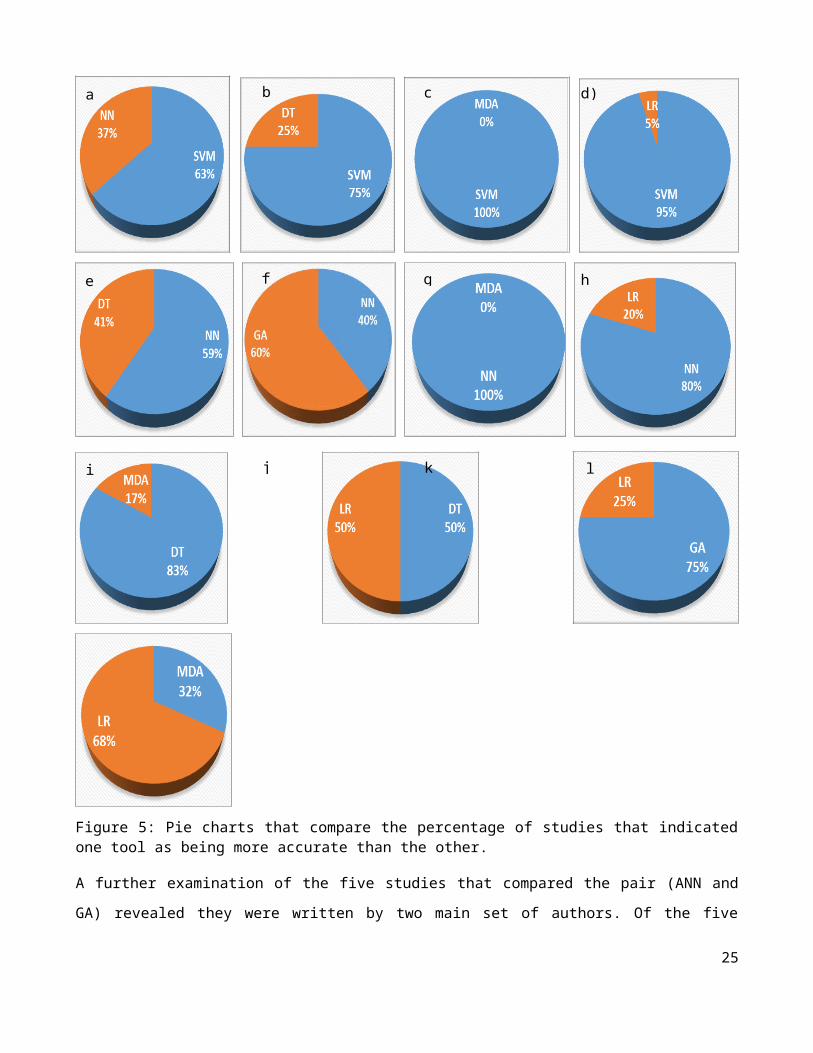
compared is 5.5 (see Table 3). To be more objective and fair in analysis, and to make a good critique, the pie
charts in Figure 5 is produced to compare the percentage of studies that rated one tool as being more accurate
than the other. It contains exactly the same pairs as Figure 4.
Figures 3, 4 and 5 all show that AI tools are more accurate than statistical tools except in Figure 5j where the
number of studies that indicated that DT is more accurate than LR and vice versa are equal. Figures 4 and 5a-d
clearly show SVM to be more accurate than any directly comparing tool though Figure 3, which is just the
average accuracy of each tool, shows ANN to be more accurate. SVM apart, Figures 4 and 5e-h similarly show
ANN to be more accurate than any comparing tool except for GA; with three against two studies confirming GA
to be more accurate.
Table 3: Matrix of number of times studies directly compared pair of tools. The tools compared above the average number of comparisons are in bold
SVM ANN DT RS GA CBR MDA LR TotalSVM - 18 10 2 3 1 8 10ANN 18 - 16 2 5 3 16 25DT 10 16 - 1 0 2 6 12RS 2 2 1 - 0 0 1 1GA 3 5 0 0 - 0 0 4CBR 1 3 2 0 0 - 2 3MDA 8 16 6 1 0 2 -- 14LR 10 25 12 1 4 3 14 -Total 53 67 21 2 4 5 14 0 165Mean Average 165/30 = 5.5
15

SVM NN
SVM DT
SVM
MDA
SVM LR NN DT NN GA
NN
MDA N
N LR DTM
DA DT LR GA LR
MDA LR
50.00
55.00
60.00
65.00
70.00
75.00
80.00
85.00
90.00Av
erag
e ac
cura
cy
Figure 4: Average accuracy results only from studies that directly compared pair of tools
Figure 5: Pie charts that compare the percentage of studies that indicated one tool as being more accurate than the other.
16
a) b) c) d)
e) f) g) h)
i) j) k) l)

A further examination of the five studies that compared the pair (ANN and GA) revealed they were written by
two main set of authors. Of the five studies, only Chen et al. (2011a), which reported ANN and SVM as being
more accurate than GA (see Table 2) could be said to have done a fair comparison since it produced the results
for ANN and GA using the same features. Chen et al. (2011b) in their study developed a robust hybrid of GA
and K-nearest neighbour (KNN) and compared it with other tools including ANN and SVM in their standalone
form thus giving GA the advantage. Divsalar et al. (2011) ‘unfairly’ used a special version of GA called linear
genetic programming (LGP) for comparison with normal ANN. Also, Divsalar et al. (2012) proposed a special
version of GA called gene expression programming (GEP), thoroughly developed its BPM using all possible
enhancements, and proved it was more accurate than models from other tools, including ANN developed with
default settings.
Similarly, Kasgari et al. (2013), which included Divsalar as the second author, used the same data as Divsalar et
al. (2012), proposed ANN for developing BPMs, thoroughly developed its model and proved it was more
accurate than other tools, including GA. Besides, GA is well known to be more suited to the process of
feature/variable selection because of its powerful global search hence its relatively infrequent use to develop
BPMs (see Figure 6); it was used for this purpose in at least four of the primary studies (Chen, 2011; Jeong et al.,
2012; Zhou et al., 2014; Liang et al. 2015) and other studies. Further “GA is a stochastic one. So, when using
GA-based models on the same training samples twice, we may get two different models, and the decision on the
same test sample may also be different. This stochastic characteristic of this method may be unacceptable for the
decision makers or the analysts” (Zhou et al. 2014, p,252). SVM and ANN can thus be claimed to be more
accurate. As noted in some of the reviewed studies (e.g. Virág and Nyitrai, 2014; Iturriaga and Sanz, 2015), this
is in line with literature as it is mostly agreed that SVM and ANN are the most accurate tools for developing
BPMs.
SVM NN DT RS GA CBR MDA LR0.00
5.00
10.00
15.00
20.00
25.00
30.00
Freq
uenc
y of
use
of t
ool (
%)
Figure 6: Percentage frequency of use of each tool
17

No study compared RS directly with GA. However, RS and ANN as well as SVM were compared directly in
two studies and RS gave a slightly better result. Like the unfair cases with GA, Yeh et al. (2014) thoroughly
developed many RS hybrid models using various enhancements and compared their average accuracy value to
single accuracy values of separate hybrids of ANN and SVM. In the second study, Virág and Nyitrai (2014),
working further from their previous study which confirmed SVM and ANN to be most accurate tools, decided to
check why non-transparent tools (i.e. SVM and ANN) were more accurate than transparent tools like RS. They
(Virág and Nyitrai 2014) initially concluded “there seems to be a kind of trade-off between the interpretability
and predictive power of bankruptcy models” (p.420) so they tried to find out what to use with “RST technique in
order to maximise the predictive power of the constructed model?” In other words, special effort was made to
improve RS accuracy while SVM and ANN were used at default level; this obviously resulted in a biased result.
Despite the effort, RS was only able to achieve the same accuracy as SVM and only a slightly higher accuracy
than ANN (Table 3). Besides, Ravi Kumar and Ravi (2007) showed in their review that RS is not as accurate as
claimed in many studies and Mckee (2003) reported a significantly reduced accuracy, compared to his previous
study, when used with what was termed a ‘more realistic’ data. RS theory is difficult to implement hence its
sparse usage (see Figure 6).
While DT’s average accuracy appears slightly higher than LR’s in Figure 4, Figure 5j shows that the number of
studies that indicated DT to be more accurate than LR and vice versa are the same. DT has generally been
confirmed to be less accurate than other AI tools like ANN and RS (Tam and Kiang, 1992; Chung and Tam
1992; McKee, 2000; Ravi Kumar and Ravi, 2007) except CBR; it (DT) has been classified as a somewhat weak
classifier in one of the reviewed studies (Heo and Yang 2014). CBR is the overall least accurate tool. Of the four
studies that used it, Chuang (2013) used it alone without comparison to any other tools. Jeong et al. (2012) and
Bemš et al. (2015) showed that it was the least accurate when compared to SVM, DT, ANN, MDA and LR
(Table 2). Only Cho et al. (2010), who presented an enhanced and hybridised CBR using DT and Mahalanobis
distance, which was the aim of the study, was able to get a better accuracy figure for CBR (hybrid) than ANN,
MDA and LR (Table 2). CBR’s low accuracy is a consequence of it not being able to handle non-linear problems
and has been deemed by some as not suitable for bankruptcy prediction (e.g. Bryant, 1997; Ravi Kumar and
Ravi, 2007). In the reviewed studies, Chuang (2013) noted that “one major factor for the poorer performance of
a stand-alone CBR model lies in its failure to separate the more important “key” attributes from those less
significant common attributes and to assign each key attribute with a different, corresponding weight” (p.184).
No wonder it is very scarcely used for BPMs (see Figure 6). Of the two statistical models, LR is clearly the more
accurate tool.
18
5.1.1.1 Error Cost
For accuracy ratings, error cost is a very important concept in bankruptcy prediction hence the tools must be
appraised with regards to it. There are two types of error in bankruptcy prediction: type I and type II. Type I
error is when a tool misclassifies a potentially bankrupt firm as being healthy. This is costlier as it could cause a
financier to loan money to a failing firm and eventually lose the money, or it could make a firm relax when it is
supposed to take active steps against insolvency. Type II error is when a tool misclassifies non-bankrupt firm as
potentially bankrupt/failing. This error is less costly. This means a tool with relatively lesser type I error is more
accurate. This, however, does not imply that type II error is unimportant as it could cost the firm its eligibility for
loans, for example.
Since the mean average of frequency of reported types I and II errors are 7.36 and 7.63 respectively (Table 1),
only the six tools that had up to 4 reporting studies and above were compared in the average types I and II error
of tools chart in Figure 7. Four is deemed not too far from seven in this case so as to allow more tools to be
compared. All error values are presented in Table 4. No study reported an error value for CBR while only one
study reported for RS. Figure 7 shows that ANN has the least average type I error followed by SVM. Coupled
with their high normal accuracy performance, they can be concluded to be the most accurate tools for bankruptcy
prediction, followed by GA. DT and LR errors are again as close as their accuracies hence their total accuracy
can be regarded to be of the same rank. However, MDA appears to be very poor with type I error hence its
accuracy can be regarded as low. ANN, DT, GA and LR have better type I errors than type II errors and vice
versa for SVM and MDA
SVM
NN
DT
GA
MDA
LR
5 7 9 11 13 15 17 19 21 23 25 27
Type I errorType II error
Figure 7: Type I versus Type II error for each tool
5.1.2 Results Interpretation
For financiers and potential clients, it is enough for a firm to be predicted as healthy or about to bankrupt.
However, for firm owners to appreciate a prediction model, the model must give an indication of where a firm is
going wrong if the firm is classified as a failing firm so that necessary steps can be taken to avoid total failure if
possible. In this context, about a quarter of the studies that used SVM and ANN highlighted the ‘black box’ 19

nature of the tools as a major problem (Table 5 and Figure 8). Other studies have also pointed out that the results
of ANN and SVM models are quite hard to understand in that weightings/coefficients they assign to the
variables are illogical and very hard to interpret (Tam and Kiang, 1992; Shin et al., 2005; Chung et al., 2008;
Ahn and Kim, 2009; Tseng and Hu, 2010).
20

Table 4: Summary of error types as reported for the tools by some of the authors
S/N Author Year SVM ANN DT RS GA MDA LRType I error
Type II error
Type I error
Type II error
Type I error
Type II error
Type I error
Type II error
Type I error
Type II error
Type I error
Type II error
Type I error
Type II error
1. Kim & Kang (2010) 17.23 30.832. Yoon & Kwon (2010) 11.34 25.143. Du Jardin (2010) 4.72 7.22 16.8 8.8 9.58 6.44. Lin et al. (2010) 5.56 5.565. Kim (2011) 4.8 12.1 47.6 27.4 22 18.46. Yang et al. (2011) 8.93 17.2 16.07 26.567. Du Jardin & Séverin (2011) 17.95 16.82 18.41 17.73 18.18 19.558. Chen et al. (2011b) 15.7 4.3 12.2 6.7 17.1 9.79. Chen et al. (2011a) 26.55 18.96 18.52 21.71 14.94 17.0210. Divsalar et al. (2012) 15.79 9.52 7.69 2011. Tsai & Cheng (2012) 19.9 6.1 12.1 16.2 13.5 17.6 17.4 9.112. Shie et al. (2012) 16.7 17.65 22.23 2513. Du Jardin & Séverin (2012) 20.1 17.4 22.1 15.5 20.1 16.614. De Andrés et al. (2012) 26.52 21.71 28.7 22.08 25.67 21.3515. Lee & Choi (2013) 12.0 6.0 24 1416. Tsai & Hsu (2013) 20.19 28.63 21.57 33.02 17.87 30.6717. Kasgari et al. (2013) 5.0 7.1418. Tsai (2014) 6.87 10.09 9.21 17.82 13.79 11.3619. Yeh et al. (2014) 11.02 3.74 18.02 4.32 26.0 1.90 10.6 3.520. Wang et al. (2014) 21.55 18.19 20.62 27.69 23.10 24.74 26.38 25.3821. Gordini (2014) 22.9 38.1 21.1 35.8 23.3 43.122. Iturria1 & Sanz (2015) 11.54 9.62 5.77 7.69 23.08 21.15 19.23 17.31
As noted by at least five of the reviewed studies (Table 5) and older studies (e.g. Ohlson, 1980; Tam and Kiang, 1992; Boritz and Kennedy, 1995;
Balcaen and Ooghe, 2006 among others), the variable coefficients in LR represent the importance of variables thus its result is transparent and help users
identify key areas of problem of a failing firm. As noted by at least five of the reviewed studies (Table 5) and some previous studies (Tam and Kiang,
1992; McKee, 2000; Greco et al., 2001; Shin and Lee, 2002; Shin et al., 2005; Ravi Kumar and Ravi, 2007), AI tools that generate decision rules for
classification (i.e. RS, CBR, GA and DT) all produce explanatory results that can be easily interpreted and understood. It appears that for AI tools, the
more accurate the tool, the less transparent the result (Figure 9). Nonetheless, McKee (2000) once spotted an inconsistency in a set of rules generated by
RS in one of his previous co-authored studies.
21

Table 5: Summary of tools that have been highlighted to be transparent, usable as hybrid, updatable, have overfitting problems etc., and year, country industry of the samples used in the reviewed studies
S/N
Author Journal of Publication Req. small sample size
Hybrid Updateable
Black box Transparent
Multicollinearity check
Overfit reported
Country
1. Tseng and Hu (2010) Expert Systems with Applications NN England2. Cho et al. (2010) Expert Systems with Applications DT Korea3. Kim & Kang (2010) Expert Systems with Applications NN NN NN Korea4. Yoon & Kwon (2010) Expert Systems with Applications NN, SVM5. Du Jardin (2010) .Neurocomputing France6. Lin et al. (2010) Journal of Marine Science and
TechnologyTaiwan
7. Gepp et al. (2010) Journal of forecasting DT US8. De Andrés et al. (2011) Knowledge-Based Systems NN Spain9. Kim (2011) Expert Systems with Applications MDA LR MDA, LR NN Korea10. Yang et al. (2011) Expert Systems with Applications SVM SVM SVM, NN SVM, NN11. Chen (2011) Neural Network World SVM SVM, GA SVM, GA Taiwan12. Divsalar et al. (2011) Expert Systems GA NN GA GA Iran13. Du Jardin & Séverin (2011) Decision Support Systems MDA, LR France14. Chen et al. (2011b) Knowledge-Based Systems GA France15. Chen et al. (2011a) Expert Systems with Applications GA16. Li et al. (2011) Knowledge-Based Systems China17. Divsalar et al. (2012) Journal of Forecasting NN GA,
LRGA Iran
18. Huang et al. (2012) Expert Systems with Applications SVM SVM, MDA
SVM, NN, DT
19. Tsai & Cheng (2012) Knowledge-Based Systems Japan20. Shie et al. (2012) Neural Computing and Applications SVM, GA LR DT USA21. Kristóf & Virág (2012) Acta Oeconomica NN DT, LR LR DT, LR22. Jeong et al. (2012). Expert Systems with Applications SVM, NN,
GASVM, NN NN Korea
23. Du Jardin & Séverin (2012) European Journal of Operational Research
MDA NN France
24. De Andrés et al. (2012) Knowledge-Based Systems NN MDA Spain25. Zhou et al. (2012) Computers & Mathematics with
ApplicationsUSA
26. Xiong et al. (2013) Expert Systems with Applications SVM27. Lee & Choi (2013) Expert Systems with Applications NN Korea28. Tsai & Hsu (2013) Journal of Forecasting NN, DT,
LR22

S/N
Author Journal of Publication Req. small sample size
Hybrid Updateable
Black box Transparent
Multicollinearity check
Overfit reported
Country
29. Callejón et al. (2013) International Journal of Computational Intelligence Systems
multiple
30. Chuang (2013) Information Sciences CBR, RS, DT
CBR
31. Ho et al. (2013) Empirical Economics US32. Arieshanti et al. (2013) TELKOMNIKA
(Telecommunication Computing Electronics and Control)
SVM, NN, LR
33. Kasgari t al. (2013). Neural Computing and Applications NN NN Iran34. Zhou et al. (2014) International Journal of Systems
ScienceSVM SVM, NN,
DT, GASVM, NN SVM, NN, DT US
35. Tsai (2014) Information Fusion NN, DT, LR
NN Australia
36. Yeh et al. (2014) Information Sciences SVM, NN, DT, RS
37. Wang et al. (2014) Expert Systems with Applications US38. Abellán & Mantas (2014) Expert Systems with Applications39. Tserng et al. (2014) Journal of Civil Engineering and
ManagementLR US
40. Yu et al. (2014) Neurocomputing SVM France41. Gordini (2014) Expert Systems with Applications LR SVM, GA Italy42. Heo & Yang (2014) Applied Soft Computing Korea43. Tsai et al. (2014) Applied Soft Computing Japan44. Virág & Nyitrai (2014) Acta Oeconomica SVM, NN, RS45. Liang et al. (2015) Knowledge-Based Systems SVM, NN,
DT, GAChina
46. Iturriaga & Sanz (2015) Expert Systems with Applications SVM, NN SVM, NN US47. Du Jardin (2015) European Journal of Operational
ResearchFrance
48. Bemš et al. (2015). Expert Systems with Applications49. Khademolqorani et al.
(2015)Mathematical Problems in Engineering
NN NN, DT Iran
23

Figure 8: Percentage of studies that complained/noted the non-transparent nature of SVM and ANN
Kim (2011) and older studies (Altman, 1968; Taffler, 1983; Tam and Kiang, 1992; Balcaen and Ooghe, 2006)
noted that although the MDA function makes MDA result look easily interpretable, the truth is that the
variables’ coefficients in the function do not represent their importance, hence results are hard to interpret.
Further, MDA sometimes yields a model with counter intuitive signs (Edum-Fotwe et al., 1996; Balcaen and
Ooghe, 2006). One of many example models is Mason and Harris’ (1979) in which a negative sign was assigned
to the profit before tax variable while representing firms with scores above cut-off as being healthy. This means
profit is bad for a firm’s health! This is obviously incomprehensible.
Figure 9: Relationship between the accuracy and transparency of results of AI tools.
One relatively popular approach to transparency problem has been to use decision rules-generating tools to select
variables and decide the importance of variables before using the very accurate black box tool for prediction.
This, from the way it is explained, is obviously not the perfect answer as it sounds like using two separate tools
for two different criteria. Kasgari et al. (2013, p.930) suggested that “to overcome this difficulty, the weights and
biases are frozen after the network was well trained and then the trained MLP models are translated into explicit
forms”, but did not explain how this is done.
24
5.1.3 Non-Deterministic Output
Unlike statistical tools and non-decision rules AI tools (i.e. ANN and SVM), AI tools that induce decision rules
for classification can produce some non-deterministic rules i.e. rules that cannot be applied to a new object
(firm) being assessed. The presence of non-deterministic rules for a new object can result into no classification
(Ahn et al., 2000; McKee, 2000; Shin and Lee, 2002; Ravi Kumar and Ravi, 2007). Of the reviewed studies,
Gordini (2014) highlighted GA as a tool that is synonymous with this problem. According to Shin and Lee
(2002), as much as 46% of new cases might not be classified by these tools (GA was used in their study).
The non-deterministic problem is encountered in this group of tools because the set of rules extracted work like a
multiple univariate system rather than a multivariate system. As a result, when any new case being assessed
cannot satisfy any or all of the rules for one reason or the other, the non-deterministic problem arises. To curtail
this problem, some studies have “reported that reduced data set (horizontally or vertically) is fed into neural
network for complementing the limitation of RS, which finally produces full prediction of new case data” (Ahn
et al., 2000, p. 68). Shin and Lee (2002) suggested the integration of multiple rules to solve the problem. For
instance, if two of eight rules (two deterministic and six non-deterministic) show a new object as unhealthy, then
the object is classified as unhealthy. Conclusively, it appears that there is no tool that clearly outperforms all
other tools in relation to all result related criteria (Figure 10).
Figure 10: Performance of tools in relation to results related criteria. There is no one tool that satisfies all the results related criteria required to develop a robust prediction model.
5.2 Data Related Criteria
5.2.1 Data Dispersion and Sample Size Capability
Data dispersion, i.e. ratio of number of non-failing sample firms to failing sample firms, is known to be key to
performance; the relative ease with which data on existing firms can be gathered usually makes them dominate
data and reduce performance. According to Du Jardin (2015), this normally means that “data that characterized 25
MDA
CBR
DT
High accuracy
Fully Deterministic
outputs
High result transparency
No tool LRANN
SVM
RS
GA

failed firms would be hidden by those that represent non-failed firms, and therefore would become rather
useless” (p.291) hence it is best to have equal dispersion (Jo et al., 1997).
MDA is quite sensitive to unequal dispersion (Balcaen and Ooghe, 2006). Compared to MDA, LR and Optimal
Estimation Theory of ANN, are better with dispersion but ANN require the least dispersion at 20% failed firms
before it could recognize pattern (Boritz et al., 1995; Du Jardin, 2015). However, no tool can perform reasonably
well at this level of dispersion i.e. 20:80 (Boritz et al., 1995). The best option is to use equally dispersed data as
most studies do. Most of the review studies have data dispersion ranging between 50-50 and 60-40 (Figure 11)
with nearly half using equally dispersed data (Table 2).
The sample size available for analysis can also influence the performance of a tool and should thus be given
serious consideration before selecting a tool. At least three of the reviewed studies (Tseng and Hu, 2010; De
Andrés et al. 2012; Zhou et al. 2014), and other studies (Haykin, 1994; Min and Lee, 2005; Shin et al., 2005;
Ravi Kumar and Ravi, 2007) clearly indicated that ANNs and MDAs need a large training sample in order to
reasonably recognize pattern and provide highly accurate classification. According to Haykin (1994), the
minimum number of sample firms required to train an ANN network is ten times the weights in the network with
an allowable error margin of 10%, i.e. over 1000 sample firms will be required to properly train a standard ANN
to make it fit for generalization. This is not too commonly implemented in many ANN studies (Shin et al., 2005)
as is evident in this study (Figure 12). However, Lee et al (2005) were able to show that ANNs can still perform
reasonably well (better than statistical models) with a small number of sample firms provided ‘a target vector is
available’. Like with ANN, a primary study (Tseng and Hu, 2010) and another study (Ravi Kumar and Ravi,
2007) have reported DT and LR to require a large data set to perform well.
CBR, RS and SVM can handle small data size (Jo et al., 1997; Olmeda, and Fernández, 1997; Ravi Kumar and
Ravi, 2007). Although Buta (1994) claimed that CBR’s accuracy increases with increase in data size, Ravi
Kumar and Ravi (2007) made it clear that it cannot handle very large data. At least four of the reviewed studies
confirmed SVM’s special ability to perform well with a small training dataset (Table 5), with Zhou et al. (2014) 26
Figure 11: Proportion of studies that used equal or almost equal data dispersion
Figure 12: Proportion of studies that used less or more than the 1000 firms sample size for ANN

noting in their wide experiment that “most SVM-based models can still keep higher performance as the size of
training samples decreases. It demonstrates that SVM models can keep good performance with small training
samples, which has been proved in many other applications also” (p.248). In Yang et al.’s (2011) experiment,
they showed that for their SVM, “the support vector number is 33 and 35 … This shows that only 33 and 35
samples from the total of 120 samples are required to achieve the appropriate identification” (p.8340). In fact,
Shin et al., (2005) did prove that SVM performs better and optimally with small training data sets as against a
large one and fairs better than ANN only when a small data set is used to train both. This SVM’s advantage is
confirmed in older studies as well (e.g. Min and Lee, 2005; Shin et al., 2005; Ravi Kumar and Ravi, 2007).
5.2.2 Variable Selection, Multicollinearity and Outliers
Statistical tools, especially LR, are highly sensitive and reactive to multicollinearity hence an effective method
of choosing non-collinear variables is normally employed for them (Edmister, 1972; Joy and Tollefson, 1975;
Back et al., 1996; Lin and Piesse, 2004; Balcaen and Ooghe, 2006). Multicollinearity can easily lead to unstable
performance and inaccurate results (Edmister, 1972; Joy and Tollefson, 1975; Balcaen and Ooghe, 2006). Before
the emergence of AI tools, the most common variable selection method is the stepwise method because of its
effectiveness in avoiding collinear variables (Altman, 1968; Back et al., 1996; Jo et al., 1997; Lin and Piesse,
2004). Its common use, over quarter of the studies used it, is usually to allow fair comparison with statistical
tools.
The reviewed studies (Chen, 2011; Chen et al., 2011b; Yang et al., 2011; Liang et al., 2015) and other previous
studies (Altman et al., 1994; Jo and Han, 1996; Chung et al., 2008) clearly indicate that AI tools, apart from
CBR, are less sensitive to multicollinearity and can perform well with almost any variable selection method.
CBR’s performance decreases with increased number of variables (Chuang, 2013). On the other hand, some
studies have claimed the higher the number of variables (usually when the multitude of variables available are
used without selecting special ones), the better for ANN and GA (Chen, 2011; Chen et al., 2011b; Liang et al.,
2015). In fact, Liang et al. (2015), who particularly investigated the effect of variable selection, concluded that
“performing feature [variable] selection does not always improve the prediction performance” (p.289) of AI
tools. However, Huang et al. (2012) feel removing irrelevant variables’ can improve performance. Although
Liang et al. (2015) found no best variable selection method in their study, they and Back et al. (1996)
recommended GA as the best selection method for AI tools. Overall, it is not uncommon to use a decision rule
generating AI tool to select variables for another AI tool as in some of the reviewed studies (Chen, 2011; Jeong
et al., 2012; Zhou et al., 2014; Liang et al. 2015) and older studies (Wallrafen et al., 1996; Back et al., 1996; Ahn
and Kim, 2009).
27

Although outliers can cause problems for any tool, LR has been particularly noted to be extremely sensitive to
outliers in at least two of the reviewed studies (Kristóf and Virág, 2012; Tsai and Cheng 2012). Outlier effects
are normally reduced by normalising variables by industry average (McKee 2000). Such normalization has
however been found to reduce accuracy of models (Tam and Kiang, 1992; Jo et al., 1997).
5.2.3 Types of Variables Applicable
This criterion was not explicitly considered by the primary studies hence only the wider literature was used to
discuss it. Although the vast majority of BPM studies use quantitative variables, usually in form of financial
ratios, the need for qualitative/explanatory/managerial variables use, as noted in many studies, cannot be
overemphasized (Argenti, 1980; Zavgren, 1985; Keasey and Watson, 1987; Abidali and Harris, 1995; Alaka et
al., 2016 among others). MDAs can use only quantitative variables (Altman, 1968; Taffler, 1982; Odom and
Sharda, 1990; Agarwa and Taffler, 2008; Chen, 2012; Bal et al., 2013 and more) while LR can use both (Ohlson,
1980; Keasey and Watson, 1987; Lin and Piesse, 2004; Cheng et al. 2006; Tseng and Hu, 2010).
ANNs and SVMs can use mainly quantitative variables but can also use qualitative variables converted to
quantitative variables using means such as the Likert scale (Cheng et al. 2006; Lin, 2009; StatSoft, 2014). All AI
tools that yield the ‘if… then,’ decision rules for bankruptcy prediction, inclusive of RS, DT, CBR and GA, use
qualitative variables and need quantitative variables to be converted to qualitative such as ‘low, medium, high’
etc. before they can be analyzed making them suitable for use of combined variables (Quinlan; 1986; Dimitras et
al., 1999; Shin and Lee, 2002; Ravi Kumar and Ravi, 2007; Martin et al., 2012). The conversion is however not
carried out by the AI and “involves dividing the original domain into subintervals which appropriately reflect
theory and knowledge of the domain” (McKee, 2000, p. 165).
5.3 Tools’ Properties Related Criteria
5.3.1 Variables Relationship Capability and Assumptions Imposed by Tools
Many independent variables used with BPM tools do not possess a linear relationship with the dependent
variable (Keasey and Watson, 1991; Balcaen and Ooghe, 2006). Three of the reviewed studies (Du Jardin and
Séverin, 2011; Divsalar et al., 2012; Du Jardin and Séverin, 2012) highlighted that MDA and LR require a linear
and logistic relationship respectively between dependent and independent variables. This means important
predictor variables with non-linear relationship to dependent variable will cause MDA to perform poorly. LR
can solve logistic and non-linear problems (Tam and Kiang, 1992; Jackson and Wood, 2013). From this review,
it appears all AI tools, except CBR (Chuang, 2013), can solve non-linear problems as identified by about a
28

quarter of the reviewed studies (e.g. Divsalar et al., 2011; Du Jardin and Séverin, 2011, 2012; Chen et al., 2011b;
Shie et al., 2012; Kasgari t al., 2013; Zhou et al., 2014; Yeh et al., 2014; among others).
Du Jardin and Séverin (2011) and other studies (Coats and Fant 1993; Lin and Piesse, 2004; Balcaen and Ooghe,
2006; Chung et al., 2008; among others) have shown that statistical tools require data to satisfy certain restrictive
assumptions for optimal performance. Some of these assumptions include multivariate normality of independent
variables, equal group variance-covariance, groups are discrete and non-overlapping etc. (Ohlson, 1980 Joy and
Tollefson, 1975; Altman, 1993; Balcaen and Ooghe, 2006). All these restrictive assumptions can barely be
satisfied together by one data set hence are violated in many studies (Richardson and Davidson, 1984; Zavgren,
1985; Chung et al., 2008). Nonetheless LR is deemed relatively less demanding compared to MDA (Altman,
1993; Balcaen and Ooghe, 2006; Jackson and Wood, 2013). On the other hand, none of the reviewed studies
noted any restrictive assumptions on data for AI tools. This is because they look to extract knowledge from
training samples or directly compare a new case to cases in the case library (Coats and Fant 1993; Shin and Lee,
2002; Lin, 2009; Jackson and Wood, 2013).
5.3.2 Sample Specificity/Overfitting Tendency and Generalizability of Tools
The common use of stepwise variable selection method and mainly financial ratios as variables for statistical
tools sometimes lead to a sample specific model where the model performs excellently on the samples used to
build it but woefully on hold out samples thereby possessing low generalizability (Edmister, 1972; Lovell, 1983;
Zavgren, 1985; Agarwal and Taffler, 2008). LR nonetheless has a relatively reasonable generalizability
(Dreiseitl and Ohno-Machado, 2002).
The equivalent of sample specificity in AI tools is called overfitting and is a common problem. There is also
underfitting which is vice versa of overfitting. It is now a norm to avoid this problem (in statistical and AI tools)
by testing models on a validation sample (and re-model if necessary) as indicated in most of the reviewed studies
(Figure 13a). Over a third of the reviewed studies also pro-actively identified this problem early (Figure 13b)
and considered it from the initial model development stage. Overfitting and underfitting are not necessarily
caused by variable selection method or variable types in the case of AI tools. Apart from the case of CBR, it is
generally known that the longer (shorter) the decision rules, the more the possibility of overfitting (underfitting)
(Clark and Niblett, 1989; Brodley and Utgoff, 1995; Ravi Kumar and Ravi, 2007; Ren, 2012). CBRs tend not to
overfit because they simply match a new case to one or more very similar cases in their library (Watson, 1997).
CBR however has poor generalization but that is due to its poor accuracy (Ravi Kumar and Ravi, 2007).
29

Figure 13: Proportion of studies that identified overfitting problem early and those that solved the problem using validation sample
Overfitting is a known problem of ANN and is as a result of overtraining the network (Min and Lee, 2005;
Cheng et al. 2006; Ahn and Kim, 2009; Tseng and Hu, 2010; Jackson and Wood, 2013). Suggestions on how to
construct more generalizable networks in ANN are given by Hertz et al. (1991). Overfitting (underfitting) in
SVM is caused by a too large (small) upper bound value, usually denoted with ‘C’ (Min and Lee, 2005; Shin et
al., 2005). Thus, finding the optimum number of training and optimum C value for ANN and SVM respectively
is key to their optimum performances. The notion that the structural risk minimization (SRM) used by SVM
helps it to reduce the possibility of overfitting and increases generalization is not well proven according to
Burges (1998). However, the tendency of overfitting in SVM is lower than in ANN and MDA (Cristianini and
Shawe-Taylor, 2000; Kim, 2003; Shin et al., 2005).
5.3.3 Model Development Time, Updatability and Integration Capability with other Tools
Although the reviewed studies did not really touch on training times, past studies have noted that training AI
tools, especially ANN and GA, can take a relatively longer time compared to statistical tools. This is because of
the iterative process of finding the best parameters for AI tools (Jo and Han, 1996; Min and Lee, 2005; Ravi
Kumar and Ravi, 2007). ANN architectures normally require many training cycles and GAs search for global
optimum, while locating and negating local minima, make them (ANN and GA) take time for model
development (Fletcher and Goss, 1993; Shin and Lee, 2002; Ravi Kumar and Ravi, 2007; Chung et al., 2008).
For SVM, the polynomial function takes a long time but its RBF function is quicker (Kim, 2003; Huang et al.,
2004). RS however does not take very long to train (Dimitras et al., 1999).
As noted in the reviewed studies, CBR and GA create the most updatable BPMs (Table7). CBR is easy to update
and quite effective after an update since all it takes is to simply add new cases to its case library and prediction
of a new case is done by finding the most similar cases(s) among all cases, old and new, in the library (Bryant,
1997; Ahn and Kim, 2009). An attempted update of a statistical BPM can lead to much reduced accuracy
(Mensah, 1984; Charitou et al., 2004). ANNs can be adaptively updated with new samples since they are known
to be robust on sample variations (Tam and Kiang, 1992; Altman, 1993; Zhang et al., 1999). However, if the
30
a) b)

situations of the new cases are significantly different for the ones used to build the model, then a new model
must be developed (Chung et al., 2008). RS is particularly very sensitive to changes in data and can really be
ineffective after an update with data that has serious sample variations (Ravi Kumar and Ravi, 2007)
AI tools are more flexible and allow integration with other tools better than statistical tools do. This is evident
from the reviewed studies as more of the studies that used AI tools produced hybrids with them than those that
used statistical tools (Figures 14a and b). The review clearly indicates that effective hybrids perform better than
standalone tools (Tsai, 2014; Zhou et al., 2014; Iturriaga and Sanz, 2015), and “usually outperforms even the
MLP [a type of ANN] and SVM procedure” (Iturriaga and Sanz 2015, p.2866). This is also confirmed in older
studies (Jo and Han, 1996; Jeng et al., 1997; Ahn et al., 2000; Ahn and Kim, 2009). “However, these hybrid
models consume more computational time” (Zhou et al. 2014, p.251) and “it is unknown which type of the
prediction models by classifier ensembles and hybrid classifiers can perform better”. (Tsai 2014, p.50)
Figure 14: Proportion of studies that integrated AI or statistical tools to form a hybrid
6.0 The Proposed Model
Figure 15 presents a diagrammatic framework, gotten from the result of this review, which serves as a guideline
for a BPM developer to select the right tool(s) that is best suited to available data and BPM preference criteria.
Virtually all tools that are used for developing BPMs can successfully make predictions. However, some tools
are more powerful in relation to certain criteria than others (see Table 6).
The framework clearly shows that to get the best performance from a BPM, the developing tool should be
selected based on the output criteria preferences and the characteristics of data available. The framework is a
very good starting point for any BPM developer and will ensure tools are not selected arbitrarily to the
disadvantage of the developer. It will also ensure the final user of the BPM, having communicated his
requirements to the model developer, gets the most appropriate BPM. For example, a BPM developer that
considers accuracy as the highest preference because of his client’s requirements, but has a very small dataset
31
a) b)

will not be wrongly choosing the highly accurate ANN for his model if this framework is used; SVM will be the
right tool in such a circumstance.
The implication of using this framework on practice is that it will allow tools to be used to the best of their
strengths and encourage BPMs to be developed in a more customized way to customer/client requirements. This
is better than to continue with the present trend of ‘one size fits all’ where a BPM is assumed to be good enough
for the very different users/clients e.g. financiers, clients, owners, government agencies, auditors etc. It will also
eliminate the time-wasting process of developing multiple BPMs with multiple tools in order to select the best
after a series of test. The implication of this work on research is that it will guide researchers in selecting the best
tool for their data and situation and help avoid the arbitrary selection of tools or selection simply based on
popularity. It will also inform researchers on the need to use hybrid tools the more if the ‘one size fits all’ tool
has to be achieved. It will hence invoke the development of new hybrid models.
Table 6: A tabular framework of tools’ performance in relation to important BPMs criteria
Statistical AI tools
MDA LR ANN SVM RS GA DT CBRAccuracy Low Mod. V. High V. High High High Mod. Low
Result transparency Low High Low Low High High High High
Can be Non-deterministic No No No No Yes Yes Yes Yes
Ability to use small Samples size Low Low Low V. high high NR low high
Data dispersion sensitivity High Normal High NR NR NR NR NR
Suitable variable selection SW SW Any Any Any Any Any Any
Multicollinearity Sensitivity High V. High Low Low Low Low Low Low
Sensitivity to outlier Mod. High Mod. Mod. Mod. Mod. Mod. Mod.
Variable type used QN Both QN (both)
QN (both)
QL (both)
(both) (both) QL (both)
Variable relationship required Linear Logistic Any Any Any Any Any Linear
Other Assumptions to be satisfied
Many Some None None None None None None
Overfitting possibility Yes Yes Yes Yes Yes Yes Yes No
Updatability Poor Poor OK - Poor OK/Good Poor Good
Ways to integrate to give hybrid Few Few Many Many Many Many Many Many
Output Mode Cut-off Binary Binary Binary DR DR DR DR
Note: All rankings are relative. NR: Not Reported SW: Stepwise V.: Very Mod: moderate QN: Quantitative QL: Qualitative DR: Decision rules.
32
Tools categoryImportant Criteria Tools
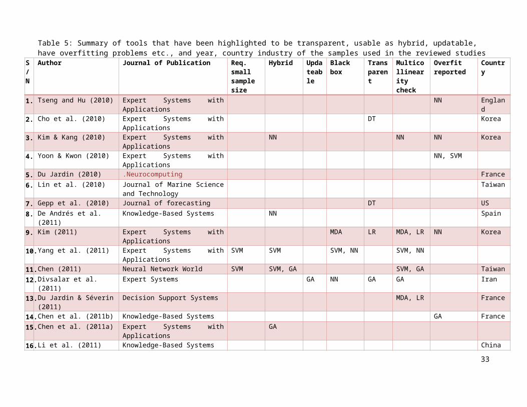
Figure 15: A framework for selection of the most suitable tools for various situationsDetermin: Deterministic Assumps: Assumptions No.: Number Poss: Possibility Relatn: RelationshipMin: Minimum Req: Required Mod.: Moderate
33

7.0 Conclusion
The bankruptcy prediction research domain continues to evolve with many new models developed using various
tools. Yet many of the tools are used with the wrong data conditions or for the wrong situation. This study used a
systematic review, to reveal how eight popular and promising tools (MDA, LR, ANN, SVM, RS, CBR, DT and
GA) perform with regard to various important criteria in the bankruptcy prediction models (BPM) study area.
Overall, it can be concluded that there is no singular tool that is predominantly better than all other tools in
relation to all identified criteria. It is however clear that each tool has its strengths and weaknesses that make it
more suited to certain situations (i.e. data characteristics, developer aim, among others) than others. The
framework presented in this study clearly provides a platform that allows a well-informed selection of tool(s)
that can best fit the situation of a model developer.
The implication of this study is that BPM developers can now make an informed decision when selecting a tool
for their model rather than make selection based on popularity or other unscholarly factors. In essence, tools will
be more regularly selected based on their strength. Another implication is that BPMs with better performance
with regards to end users’ requirement will be more commonly developed. This is better than to continue with
the present trend of ‘one size fits all’ where a BPM tool is assumed to be good enough for the very different
users/clients (e.g. financiers, clients, owners, government agencies, auditors, among others) that need them. The
framework in this study will also reduce the time-wasting process of developing many BPMs with different tools
in order to select the best after a series of test; only the tools that best fit a developer’s situation will be used and
compared.
Future studies should consider possibilities of making ANN and SVM results interpretable since they appear to
be the most accurate tools and satisfy a number of criteria for BPM. The very best overall model that will
outperform all others in relation to all or most criteria, though not yet found, might come in the form of a hybrid
of tools. Future research should thus, on one hand, explore various hybrids with the aim of developing the best
hybrid that can achieve this fit. On the other hand, future studies should consider use of more sophisticated tools
like Bart machine, extremely randomized trees, gradient boosting machine and extreme Gradient Boosting
among others, as they might be the answer. As tools that can handle qualitative variables have been exposed in
this study, future studies should consider the inclusion of qualitative variables in their BPM development as
suggested in many studies (e.g. Argenti, 1980; Abidali and Harris, 1995; Alaka et al., 2017; among others).
Further, future studies should look to combine qualitative and qualitative variables using these tools, with a view
of developing better performing BPMs. Finally, future research should attempt to confirm/falsify the SVM tool’s
excellent capability to make predictions on small data size since it is generally known that the larger the data, the
better.
34

References
Abellán, J., and Mantas, C. J. (2014). Improving experimental studies about ensembles of classifiers for
bankruptcy prediction and credit scoring. Expert Systems with Applications, 41 (8), pp. 3825-3830.
Abidali, A. F., and Harris, F. (1995). A methodology for predicting failure in the construction industry.
Construction Management and Economics, 13 (3), pp. 189–196.
Agarwal, V., and Taffler, R. (2008). Comparing the performance of market-based and accounting-based
bankruptcy prediction models. Journal of Banking and Finance, 32 (8), pp. 1541-1551.
Ahn, B. S., Cho, S. S., and Kim, C. Y. (2000). The integrated methodology of rough set theory and artificial
neural network for business failure prediction. Expert Systems with Applications, 18 (2), pp. 65-74.
Ahn, H., and Kim, K. J. (2009). Bankruptcy prediction modeling with hybrid case-based reasoning and genetic
algorithms approach. Applied Soft Computing, 9 (2), pp. 599-607.
Alaka, H, Oyedele, L, Toriola-Coker, O, Owolabi, H, Akinade, O, Bilal, M and Ajayi, S (2015) Methodological
approach of construction businesses failure prediction studies: A review In: Raidén, A B and Aboagye-
Nimo, E (Eds) Procs 31st Annual ARCOM Conference, 7-9 September 2015, Lincoln, UK, Association of
Researchers in Construction Management, pp. 1291-1300.
Alaka, H. A., Oyedele, L. O., Owolabi, H. A., Ajayi, S. O., Bilal, M., & Akinade, O. O. (2016). Methodological
approach of construction business failure prediction studies: a review. Construction Management and
Economics, 34(11), 808-842.
Alaka, H. A., Oyedele, L. O., Owolabi, H. A., Oyedele, A. A., Akinade, O. O., Bilal, M., & Ajayi, S. O. (2017).
Critical factors for insolvency prediction: towards a theoretical model for the construction
industry. International Journal of Construction Management, 17(1), 25-49.
Altman E.I. (1968). Financial ratios discriminant analysis and the prediction of corporate bankruptcy, The
Journal of Finance, 23 (4), pp. 589-609
Altman E. (1993). Corporate Financial Distress and Bankruptcy. 2nd ed. New York: John Wiley and Sons.
Altman, E. I., Marco, G., and Varetto, F. (1994). Corporate distress diagnosis: comparisons using linear
discriminant analysis and neural networks (the Italian experience). Journal of banking and finance, 18 (3),
505-529
Appiah, K. O., Chizema, A., and Arthur, J. (2015). Predicting corporate failure: a systematic literature review of
methodological issues. International Journal of Law and Management, 57 (5), pp. 461-485.
Argenti, J. (1980). Practical Corporate Planning. London: Allen and Unwin,
35

Arieshanti, I., Purwananto, Y., Ramadhani, A., Nuha, M. U., and Ulinnuha, N. (2013). Comparative Study of
Bankruptcy Prediction Models. TELKOMNIKA (Telecommunication Computing Electronics and
Control), 11 (3), pp. 591-596.
Aziz, M. A. and Dar, H. A. (2006). Predicting corporate bankruptcy: where we stand? Corporate Governance, 6
(1), pp. 18-33.
Back, B., Laitinen, T., and Sere, K. (1996). Neural networks and genetic algorithms for bankruptcy
predictions. Expert Systems with Applications, 11 (4), pp. 407-413.
Bal, J., Cheung, Y., and Wu, H. C. (2013). Entropy for business failure prediction: an improved prediction model for the construction industry. Advances in Decision Sciences, 2013 (2013), pp. 1-14.
Balcaen, S., and Ooghe, H. (2006). 35 years of studies on business failure: an overview of the classic statistical methodologies and their related problems. The British Accounting Review, 38 (1), pp. 63-93.
Beaver, W. H. (1966). Financial ratios as predictors of failure. Journal of Accounting Research, 4 (1966), pp. 71-111.
Beaver, W. H., McNichols, M. F., & Rhie, J. W. (2005). Have financial statements become less informative? Evidence from the ability of financial ratios to predict bankruptcy. Review of Accounting studies, 10 (1), pp. 93-122.
Bemš, J., Starý, O., Macaš, M., Žegklitz, J., and Pošík, P. (2015). Innovative default prediction approach. Expert Systems with Applications, 42 (17), pp. 6277-6285.
Boritz, J.E. and Kennedy, D. B. (1995). Effectiveness of neural network types for prediction of business failure. Expert Systems with Applications, 9 (4), pp. 503-512.
Boritz, J. E., Kennedy, D. B. and Albuquerque A.M. (1995). Predicting corporate failure using a neural network approach. Intelligent Systems in Accounting, Finance and Management, 4 (2), pp. 95-111.
Brodley, C. E., and Utgoff, P. E. (1995). Multivariate decision trees. Machine Learning, 19 (1), pp. 45-77.
Bryant, S. M. (1997). A case‐based reasoning approach to bankruptcy prediction modeling. Intelligent Systems in Accounting, Finance and Management, 6 (3), pp. 195-214.
Burges, C. J. (1998). A tutorial on support vector machines for pattern recognition. Data Mining and Knowledge Discovery, 2 (2), pp. 121-167.
Buta, P. (1994). Mining for financial knowledge with CBR. Ai Expert, 9 (2), pp. 34-41.
Callejón, A. M., Casado, A. M., Fernández, M. A., and Peláez, J. I. (2013). A system of insolvency prediction for industrial companies using a financial alternative model with neural networks. International Journal of Computational Intelligence Systems, 6 (1), pp. 29-37.
Charitou, A., Neophytou, E., and Charalambous, C. (2004). Predicting corporate failure: empirical evidence for the UK. European Accounting Review, 13 (3), pp. 465-497.
Chen, H. L., Yang, B., Wang, G., Liu, J., Xu, X., Wang, S. J., and Liu, D. Y. (2011a). A novel bankruptcy prediction model based on an adaptive fuzzy k-nearest neighbor method. Knowledge-Based Systems, 24 (8), pp. 1348-1359.
36

Chen, J. H. (2012). Developing SFNN models to predict financial distress of construction companies. Expert Systems with Applications, 39 (1), pp. 823-827.
Chen, M. Y. (2011). A hybrid model for business failure prediction-utilization of particle swarm optimization and support vector machines. Neural Network World, 21 (2), pp. 129-152.
Chen, N., Ribeiro, B., Vieira, A. S., Duarte, J., and Neves, J. C. (2011b). A genetic algorithm-based approach to cost-sensitive bankruptcy prediction. Expert Systems with Applications, 38 (10), pp. 12939-12945.
Cheng, C.B., Chen, C. L. and Fu, C.J. (2006). Financial distress prediction by a radial basis function network with logit analysis learning. Computers and Mathematics with Applications, 51 (3–4), pp. 579–588.
Cho, S., Hong, H., and Ha, B. C. (2010). A hybrid approach based on the combination of variable selection using decision trees and case-based reasoning using the Mahalanobis distance: For bankruptcy prediction. Expert Systems with Applications, 37 (4), pp. 3482-3488.
Chuang, C. L. (2013). Application of hybrid case-based reasoning for enhanced performance in bankruptcy prediction. Information Sciences, 236 (2013), pp. 174-185.
Chung, H.M.M., and Tam, K.Y. (1993). A Comparative Analysis of Inductive‐Learning Algorithms. Intelligent Systems in Accounting, Finance and Management, 2 (1), pp. 3-18.
Chung, K. C., Tan, S. S. and Holdsworth, D. K. (2008). Insolvency prediction model using multivariate discriminant analysis and artificial neural network for the finance industry in New Zealand. International Journal of Business and Management, 39 (1), pp. 19-28.
Clark, P. and Niblett, T. (1989). The CN2 induction algorithm. Machine Learning, 3 (4), pp. 261-283.
Coats, P. K., and Fant, L. F. (1993). Recognizing financial distress patterns using a neural network tool. Financial Management, 22 (3), pp. 142-155.
Cristianini, N., and Shawe-Taylor, J. (2000). An Introduction to Support Vector Machines and other Kernel-Based Learning Methods. Cambridge; Cambridge university press.
De Andrés, J., Lorca, P., de Cos Juez, F. J., and Sánchez-Lasheras, F. (2011). Bankruptcy forecasting: A hybrid approach using Fuzzy c-means clustering and Multivariate Adaptive Regression Splines (MARS). Expert Systems with Applications, 38 (3), pp. 1866-1875.
De Andrés, J., Landajo, M., and Lorca, P. (2012). Bankruptcy prediction models based on multinorm analysis: An alternative to accounting ratios. Knowledge-Based Systems, 30, pp. 67-77.
Dimitras, A. I., Slowinski, R., Susmaga, R., and Zopounidis, C. (1999). Business failure prediction using rough sets. European Journal of Operational Research, 114 (2), 263-280.
Divsalar, M., Firouzabadi, A. K., Sadeghi, M., Behrooz, A. H., and Alavi, A. H. (2011). Towards the prediction of business failure via computational intelligence techniques. Expert Systems, 28 (3), pp.209-226.
Divsalar, M., Roodsaz, H., Vahdatinia, F., Norouzzadeh, G., and Behrooz, A. H. (2012). A Robust Data ‐Mining Approach to Bankruptcy Prediction. Journal of Forecasting, 31 (6), pp.504-523.
Dreiseitl, S., and Ohno-Machado, L. (2002). Logistic regression and artificial neural network classification models: a methodology review. Journal of biomedical informatics, 35 (5), pp. 352-359
Du Jardin, P. (2010). Predicting bankruptcy using neural networks and other classification methods: The influence of variable selection techniques on model accuracy. Neurocomputing, 73 (10), pp .2047-2060.
37

Du Jardin, P. (2015). Bankruptcy prediction using terminal failure processes. European Journal of Operational Research, 242 (1), pp. 286-303.
Du Jardin, P., and Séverin, E. (2011). Predicting corporate bankruptcy using a self-organizing map: An empirical study to improve the forecasting horizon of a financial failure model. Decision Support Systems, 51 (3), pp. 701-711.
Du Jardin, P., and Séverin, E. (2012). Forecasting financial failure using a Kohonen map: A comparative study to improve model stability over time.European Journal of Operational Research, 221 (2), pp. 378-396.
Edmister, R. O. (1972). An empirical test of financial ratio analysis for small business failure prediction. Journal of Financial and Quantitative Analysis, 7 (02), pp. 1477-1493.
Edum-Fotwe, F., Price, A. and Thorpe, A. (1996) A review of financial ratio tools for predicting contractor insolvency. Construction Management and Economics, 14 (1996), pp. 189-198.
Fletcher, D. and Goss, E. (1993). Forecasting with neural networks: an application using bankruptcy data. Information and Management, 24 (3), pp. 159-167.
Gepp, A., Kumar, K., and Bhattacharya, S. (2010). Business failure prediction using decision trees. Journal of forecasting, 29 (6), pp. 536-555.
Gordini, N. (2014). A genetic algorithm approach for SMEs bankruptcy prediction: Empirical evidence from Italy. Expert Systems with Applications, 41 (14), pp. 6433-6445.
Greco, S., Matarazzo, B., and Slowinski, R. (2001). Rough sets theory for multicriteria decision analysis. European Journal of Operational Research, 129 (1), pp. 1-47.
Hafiz, A., Lukumon, O., Muhammad, B., Olugbenga, A., Hakeem, O., and Saheed, A. (2015, March). Bankruptcy Prediction of Construction Businesses: Towards a Big Data Analytics Approach. In Big Data Computing Service and Applications (BigDataService), 2015 IEEE First International Conference on (pp. 347-352). IEEE.
Haykin, S. (1994). Neural Networks: A Comprehensive Foundation. New York: Mc Millan.
Heo, J., and Yang, J. Y. (2014). AdaBoost based bankruptcy forecasting of Korean construction companies. Applied Soft Computing, 24, PP. 494-499.
Hertz, J., Krogh, A. and Palmer, R. (1991). Introduction to the Theory of Neural Computing. New York: Addison Wesley.
Higgins, J. P. (Ed.). (2008). Cochrane handbook for systematic reviews of interventions (Vol. 5). Chichester, England: Wiley-Blackwell.
Hillegeist, S. A., Keating, E. K., Cram, D. P., and Lundstedt, K. G. (2004). Assessing the probability of bankruptcy. Review of accounting studies, 9 (1), pp.5-34.
Ho, C. Y., McCarthy, P., Yang, Y., and Ye, X. (2013). Bankruptcy in the pulp and paper industry: market’s reaction and prediction. Empirical Economics, 45 (3), pp. 1205-1232.
Huang, S. C., Tang, Y. C., Lee, C. W., and Chang, M. J. (2012). Kernel local Fisher discriminant analysis based manifold-regularized SVM model for financial distress predictions. Expert Systems with Applications, 39 (3), pp. 3855-3861.
38

Huang, Z., Chen, H., Hsu, C. J., Chen, W. H., and Wu, S. (2004). Credit rating analysis with support vector machines and neural networks: a market comparative study. Decision Support Systems, 37 (4), pp. 543-558.
Iturriaga, F. J. L., and Sanz, I. P. (2015). Bankruptcy visualization and prediction using neural networks: A study of US commercial banks. Expert Systems with Applications, 42 (6), p. 2857-2869.
Jackson, R. H., and Wood, A. (2013). The performance of insolvency prediction and credit risk models in the UK: a comparative study. The British Accounting Review, 45 (3), pp. 183-202.
Jeng, B., Jeng, Y. M., and Liang, T. P. (1997). FILM: a fuzzy inductive learning method for automated knowledge acquisition. Decision Support Systems, 21 (2), pp. 61-73.
Jeong, C., Min, J. H., and Kim, M. S. (2012). A tuning method for the architecture of neural network models incorporating GAM and GA as applied to bankruptcy prediction. Expert Systems with Applications, 39 (3), pp. 3650-3658.
Jo, H., and Han, I. (1996). Integration of case-based forecasting, neural network, and discriminant analysis for bankruptcy prediction. Expert Systems with applications, 11 (4), pp. 415-422.
Jo, H., Han, I., and Lee, H. (1997). Bankruptcy prediction using case-based reasoning, neural networks, and discriminant analysis. Expert Systems with Applications, 13 (2), pp. 97-108.
Joy, O. M., and Tollefson, J. O. (1975). On the financial applications of discriminant analysis. Journal of Financial and Quantitative Analysis, 10 (5), pp. 723-739.
Kasgari, A. A., Divsalar, M., Javid, M. R., and Ebrahimian, S. J. (2013). Prediction of bankruptcy Iranian corporations through artificial neural network and Probit-based analyses. Neural Computing and Applications, 23 (3-4), pp. 927-936.
Keasey, K., and Watson, R. (1987). Non‐financial symptoms and the prediction of small company failure: a test of Argenti's hypotheses. Journal of Business Finance and Accounting, 14 (3), pp. 335-354.
Keasey, K., and Watson, R. (1991). Financial distress prediction models: a review of their usefulness 1. British journal of Management, 2 (2), pp. 89-102.
Khademolqorani, S., Zeinal Hamadani, A., and Mokhatab Rafiei, F. (2015). A Hybrid Analysis Approach to Improve Financial Distress Forecasting: Empirical Evidence from Iran. Mathematical Problems in Engineering, 2015.
Khan, K. S., Kunz, R., Kleijnen, J., and Antes, G. (2003). Five steps to conducting a systematic review. Journal of the Royal Society of Medicine, 96 (3), pp. 118-121.
Kim, K. J. (2003). Financial time series forecasting using support vector machines. Neurocomputing, 55 (1), pp. 307-319.
Kim, M. J., and Kang, D. K. (2010). Ensemble with neural networks for bankruptcy prediction. Expert Systems with Applications, 37 (4), pp. 3373-3379.
Kim, S. Y. (2011). Prediction of hotel bankruptcy using support vector machine, artificial neural network, logistic regression, and multivariate discriminant analysis. The Service Industries Journal, 31 (3), pp. 441-468.
Kolodner, J. (1993). Case-Based Reasoning. San Francisco, California: Morgan Kaufmann Publishers Inc.
39

Koyuncugil, A. S., and Ozgulbas, N. (2012). Financial early warning system model and data mining application for risk detection. Expert Systems with Applications, 39 (6), pp. 6238-6253.
Kristóf, T., and Virág, M. (2012). Data reduction and univariate splitting—Do they together provide better corporate bankruptcy prediction?. Acta Oeconomica, 62 (2), pp. 205-228.
Langford, D., Iyagba, R. and Komba, D.M. (1993) Prediction of solvency in construction companies, Construction Management and Economics, 11 (1993), pp. 317-325
Lee, K., Booth, D., and Alam, P. (2005). A comparison of supervised and unsupervised neural networks in predicting bankruptcy of Korean firms. Expert Systems with Applications, 29 (1), pp. 1-16.
Lee, S., and Choi, W. S. (2013). A multi-industry bankruptcy prediction model using back-propagation neural network and multivariate discriminant analysis.Expert Systems with Applications, 40(8), 2941-2946.
Li, H., Lee, Y. C., Zhou, Y. C., and Sun, J. (2011). The random subspace binary logit (RSBL) model for bankruptcy prediction. Knowledge-Based Systems, 24 (8), pp. 1380-1388.
Liang, D., Tsai, C. F., and Wu, H. T. (2015). The effect of feature selection on financial distress prediction. Knowledge-Based Systems, 73, pp. 289-297.
Lin, F., Liang, D., and Chu, W. S. (2010). The role of non-financial features related to corporate governance in business crisis prediction. Journal of Marine Science and Technology, 18 (4), pp.504-513.
Lin, F. Y., and McClean, S. (2001). A data mining approach to the prediction of corporate failure. Knowledge-Based Systems, 14 (3), pp. 189-195.
Lin, L., and Piesse, J. (2004). Identification of corporate distress in UK industrials: a conditional probability analysis approach. Applied Financial Economics, 14 (2), pp. 73-82.
Lin, T. H. (2009). A cross model study of corporate financial distress prediction in Taiwan: multiple discriminant analysis, logit, probit and neural networks models. Neurocomputing, 72 (16), pp. 3507-3516.
Lovell, M.C. (1983). Data mining. Review of Economic Statistics 65 (1), pp. 1–12.
Martens, D., Van Gestel, T., De Backer, M., Haesen, R., Vanthienen, J., and Baesens, B. (2010). Credit rating prediction using ant colony optimization.Journal of the Operational Research Society, 61 (4), pp. 561-573.
Martin, A., Manjula, M., and Venkatesan, D. V. P. (2011). A business intelligence model to predict bankruptcy using financial domain ontology with association rule mining algorithm. International Journal of Computer Science Issues, 8 (3), pp. 1694-0814.
Martin, A., Balaji, S. and Venkatesan V.P. (2012). Effective prediction of bankruptcy based on the qualitative factors using FID3 algorithm. International Journal of Computer Applications (0975 – 8887), 43 (21), pp. 28-32.
Mason, R. J. and Harris, F. C. (1979). Predicting company failure in the construction industry. In: Proceedings of Institution of Civil Engineers, 01 May 1979, 66 (2), London: Thomas Telford, pp. 301-307.
Mensah, Y. M. (1984). An examination of the stationarity of multivariate bankruptcy prediction models: a methodological study. Journal of Accounting Research, 22 (1), pp. 380-395.
McKee, T. E. (2000). Developing a bankruptcy prediction model via rough sets theory. Intelligent Systems in Accounting, Finance and Management, 9 (3), pp. 159-173.
40

McKee, T. E. (2003). Rough sets bankruptcy prediction models versus auditor signalling rates. Journal of Forecasting, 22 (8), pp. 569-586.
Min, J. H., and Lee, Y. C. (2005). Bankruptcy prediction using support vector machine with optimal choice of kernel function parameters. Expert Systems with Applications, 28 (4), pp. 603-614.
Min, S. H., Lee, J., and Han, I. (2006). Hybrid genetic algorithms and support vector machines for bankruptcy prediction. Expert systems with applications, 31 (3), pp. 652-660.
Nasir, M. L., John, R. I., Bennett, S. C., Russell, D. M., and Patel, A. (2000). Predicting corporate bankruptcy using artificial neural networks. Journal of Applied Accounting Research, 5 (3), pp. 30-52.
Odom, M. D., and Sharda, R. (1990). A neural network model for bankruptcy prediction. In: IJCNN International Joint Conference on Neural Networks. San Diego, California, 17-21 June 1990. IEEE, pp. 163-168.
Ohlson, J.A. (1980). Financial ratios and the probabilistic prediction of bankruptcy. Journal of Accounting Research, 18 (1) pp. 109-131.
Olmeda, I., and Fernández, E. (1997). Hybrid classifiers for financial multicriteria decision making: the case of bankruptcy prediction. Computational Economics, 10 (4), pp. 317-335.
Pawlak, Z. (1982). Rough sets. International Journal of Computer and Information Sciences, 11 (5), pp. 341-356.
Quinlan, J. R. (1986). Induction of decision trees. Machine Learning, 1 (1), pp. 81-106.
Quinlan, J. R. (1993). Programs for machine learning. Morgan Kaufmann Series in Machine Learning. San Mateo, CA.
Ravi Kumar, P., and Ravi, V. (2007). Bankruptcy prediction in banks and firms via statistical and intelligent techniques–A review. European Journal of Operational Research, 180 (1), pp. 1-28.
Ren, D. (2012). Application attributes reduction of rough set in power system for fault diagnosis. Journal of Convergence Information Technology, 7 (13), pp. 300-308
Richardson, F. M., and Davidson, L. F. (1984). On linear discrimination with accounting ratios. Journal of Business Finance and Accounting, 11 (4), pp. 511-525.
Schlosser, R. W. (2007). Appraising the quality of systematic reviews. Focus: Technical Briefs, (17), pp. 1-8.
Shi, G. (2013). Data Mining and Knowledge Discovery for Geoscientists. San Diego: Elsevier
Shie, F. S., Chen, M. Y., and Liu, Y. S. (2012). Prediction of corporate financial distress: an application of the America banking industry. Neural Computing and Applications, 21 (7), pp. 1687-1696.
Shin, K. S., and Lee, Y. J. (2002). A genetic algorithm application in bankruptcy prediction modeling. Expert Systems with Applications, 23 (3), pp. 321-328.
Shin, K. S., Lee, T. S., and Kim, H. J. (2005). An application of support vector machines in bankruptcy prediction model. Expert Systems with Applications, 28 (1), pp. 127-135.
Smith, V., Devane, D., Begley, C. M., and Clarke, M. (2011). Methodology in conducting a systematic review of systematic reviews of healthcare interventions. BMC medical research methodology, 11 (1), 15.
41

StatSoft (2014). Support Vector Machines (SVM) [online]. Available from: http://www.statsoft.com/Textbook/Support-Vector-Machines#index [Accessed 26 September 2016]
Stenbacka, C. (2001). Qualitative research requires quality concepts of its own. Management Decision, 39 (7), pp. 551-556.
Sun, J., Li, H., Huang, Q. H., and He, K. Y. (2014). Predicting financial distress and corporate failure: A review from the state-of-the-art definitions, modeling, sampling, and featuring approaches. Knowledge-Based Systems, 57, 41-56.
Taffler, R. J. (1982). Forecasting company failure in the UK using discriminant analysis and financial ratio data. Journal of the Royal Statistical Society. Series A (General), 342-358.
Taffler, R. J. (1983). The assessment of company solvency and performance using a statistical model. Accounting and Business Research, 13 (52), pp. 295-308.
Tam, K. Y., and Kiang, M. Y. (1992). Managerial applications of neural networks: the case of bank failure predictions. Management science, 38 (7), pp. 926-947.
Tranfield, D. R., Denyer, D., and Smart, P. (2003). Towards a methodology for developing evidence-informed management knowledge by means of systematic review. British journal of management, 14, pp. 207-222.
Trochim, W.M. and Donnelly, J.P. (2006). The Research Methods Knowledge Base, 3rd ed. Ohio: Atomic Dog Publishing.
Tsai, C. F. (2014). Combining cluster analysis with classifier ensembles to predict financial distress. Information Fusion, 16, pp. 46-58.
Tsai, C. F., and Cheng, K. C. (2012). Simple instance selection for bankruptcy prediction. Knowledge-Based Systems, 27 (2012), pp. 333-342.
Tsai, C. F., and Hsu, Y. F. (2013). A Meta‐learning Framework for Bankruptcy Prediction. Journal of Forecasting, 32 (2), pp. 167-179.
Tsai, C. F., Hsu, Y. F., and Yen, D. C. (2014). A comparative study of classifier ensembles for bankruptcy prediction. Applied Soft Computing, 24, pp. 977-984.
Tseng, F. M., and Hu, Y. C. (2010). Comparing four bankruptcy prediction models: logit, quadratic interval logit, neural and fuzzy neural networks. Expert Systems with Applications, 37 (3), pp. 1846-1853.
Tserng, H. P., Chen, P. C., Huang, W. H., Lei, M. C., and Tran, Q. H. (2014). Prediction of default probability for construction firms using the logit model .Journal of Civil Engineering and Management, 20 (2), pp. 247-255.
Vapnik, V. (1998). Statistical Learning Theory (Vol. 2). New York: Springer
Virág, M., and Nyitrai, T. (2014). Is there a trade-off between the predictive power and the interpretability of bankruptcy models? The case of the first Hungarian bankruptcy prediction model. Acta Oeconomica, 64 (4), pp. 419-440.
Wang, G., Ma, J., and Yang, S. (2014). An improved boosting based on feature selection for corporate bankruptcy prediction. Expert Systems with Applications, 41 (5), pp. 2353-2361.
Wallrafen, J., Protzel, P., and Popp, H. (1996). Genetically optimized neural network classifiers for bankruptcy prediction-an empirical study. In: Proceedings of the Twenty-Ninth Hawaii International Conference on
42

System Sciences. Hawaii, USA, 3-6 Jan. 1996. Washington: IEEE Computer Society Press, cop., Vol. 2, pp. 419-426.
Watson, I. (1997). Applying case-based reasoning: techniques for enterprise systems. San Francisco, California: Morgan Kaufmann Publishers Inc.
Won, C., Kim, J., and Bae, J. K. (2012). Using genetic algorithm based knowledge refinement model for dividend policy forecasting. Expert Systems with Applications, 39 (18), pp. 13472-13479.
Wilson, R. L., and Sharda, R. (1994). Bankruptcy prediction using neural networks. Decision Support Systems, 11(5), pp. 545-557.
Xiong, T., Wang, S., Mayers, A., and Monga, E. (2013). Personal bankruptcy prediction by mining credit card
data. Expert Systems with Applications, 40 (2), pp. 665-676.
Xu, M., and Zhang, C. (2009). Bankruptcy prediction: the case of Japanese listed companies. Review of
Accounting Studies, 14 (4), pp. 534-558.
Yang, Z., You, W., and Ji, G. (2011). Using partial least squares and support vector machines for bankruptcy
prediction. Expert Systems with Applications, 38 (7), pp. 8336-8342.
Yeh, C. C., Chi, D. J., and Lin, Y. R. (2014). Going-concern prediction using hybrid random forests and rough
set approach. Information Sciences, 254, pp. 98-110.
Yoon, J. S., and Kwon, Y. S. (2010). A practical approach to bankruptcy prediction for small businesses:
Substituting the unavailable financial data for credit card sales information. Expert systems with
Applications, 37 (5), pp. 3624-3629.
Yu, Q., Miche, Y., Séverin, E., and Lendasse, A. (2014). Bankruptcy prediction using extreme learning machine
and financial expertise. Neurocomputing, 128, 296-302.
Zavgren, C. V. (1985). Assessing the vulnerability to failure of American industrial firms: a logistic
analysis. Journal of Business Finance and Accounting, 12 (1), pp. 19-45.
Zhang, G., Hu, M.Y., Patuwo, E.B. and Indro, D.C. (1999). Artificial neural networks in bankruptcy prediction:
general framework and cross-validation analysis. European Journal of Operational Research, 116 (1), pp.
16-32.
Zhou, L., Lai, K. K., and Yen, J. (2012). Empirical models based on features ranking techniques for corporate
financial distress prediction. Computers and Mathematics with Applications, 64 (8), pp. 2484-2496.
Zhou, L., Lai, K. K., and Yen, J. (2014). Bankruptcy prediction using SVM models with a new approach to
combine features selection and parameter optimisation. International Journal of Systems Science, 45 (3),
pp. 241-253.
43

Zurada, J. M., Malinowski, A., and Cloete, I. (1994). Sensitivity analysis for minimization of input data
dimension for feedforward neural network. In: IEEE International Symposium on Circuits and Systems,
ISCAS’94, London, United Kingdom, 30 May – 2 June, 1994. Vol. 6, pp. 447-450.
44
![€¦ · Web view2009. 4. 23. · [Cr2O72-] Reverse Rate. A. increases increases. B. increases decreases. C. decreases decreases. D. decreases increases. 31. A small amount of H2SO4](https://img.pdfslide.us/doc/110x75/608f2c47b9e3f5096f2e5efc/web-view-2009-4-23-cr2o72-reverse-rate-a-increases-increases-b-increases.jpg)