MIT OpenCourseWare ____________http://ocw.mit.edu

2.830J / 6.780J / ESD.63J Control of Manufacturing Processes (SMA 6303)Spring 2008

For information about citing these materials or our Terms of Use, visit: ________________http://ocw.mit.edu/terms.

1Manufacturing

Control of Manufacturing Processes

Subject 2.830/6.780/ESD.63Spring 2008Lecture #7

Shewhart SPC & Process Capability

February 28, 2008

2Manufacturing

Applying Statistics to Manufacturing:The Shewhart Approach

Text removed due to copyright restrictions. Please see the Abstract of Shewhart, W. A. “The Applications of Statistics as an Aid in Maintaining Quality of a Manufactured Product.” Journal of the American Statistical Association 20 (December 1925): 546-548.

3Manufacturing

Applying Statistics to Manufacturing:The Shewhart Approach

Text removed due to copyright restrictions. Please see the Abstract of Shewhart, W. A. “The Applications of Statistics as an Aid in Maintaining Quality of a Manufactured Product.” Journal of the American Statistical Association 20 (December 1925): 546-548.

4Manufacturing

Applying Statistics to Manufacturing:The Shewhart Approach (circa 1925)*

• All Physical Processes Have a Degree of Natural Randomness

• A Manufacturing Process is a Random Process if all “Assignable Causes” (identifiable disturbances) are eliminated

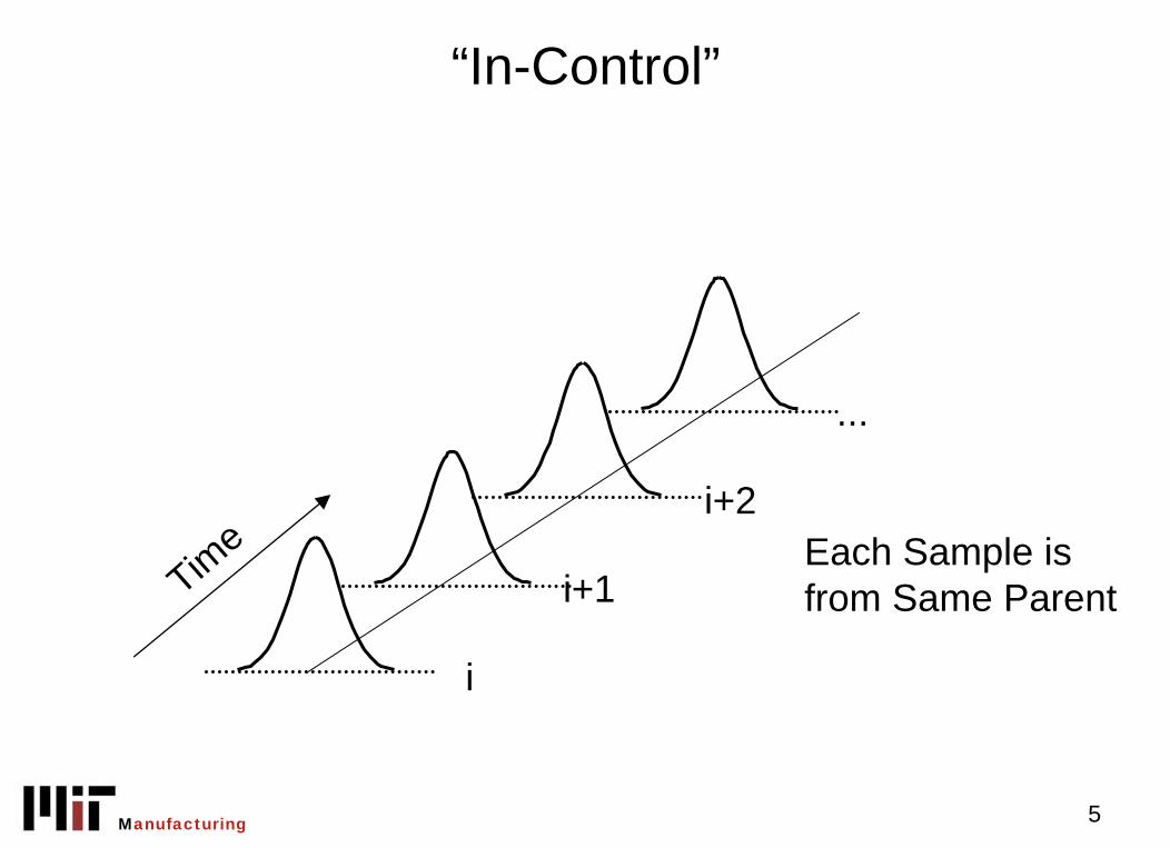
• A Process is “In Statistical Control” if only “Common Causes” (Purely Random Effects) are present.

5Manufacturing

“In-Control”

i

i+1

i+2

...

Each Sample is from Same ParentTim

e

6Manufacturing

“Not In-Control”

i

i+1

i+2

...

The Parent Distribution is NotThe Same at Each Sample

Time

7Manufacturing

“Not In-Control”

...

Time

Mean Shift

Mean Shift + Variance Change

Bi-Modal

What will appear in “Samples”?

8Manufacturing

Xbar and S Charts

• Shewhart:– Plot sequential average of process

• Xbar chart• Distribution?

– Plot sequential sample standard deviation• S chart• Distribution?

9Manufacturing

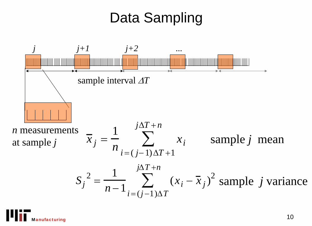
n measurementsat sample j

sample interval ΔT

• A sequential sample of size n

• Take at intervals ΔT

• Sample index j

Data Sampling and Sequential Averages

• Given a sequence of process outputs xi:

j j+1 j+2 ...

10Manufacturing

x j =1n

xii = ( j− 1) ΔT +1

jΔT + n

∑ sample j mean

Sj2 =

1n − 1

(xii = ( j −1)ΔT

jΔT +n

∑ − x j )2 sample j variance

Data Sampling

n measurementsat sample j

sample interval ΔT

j j+1 j+2 ...

11Manufacturing

n measurementsat sample j

Subgroups

j j+1 j+2 ...

• Within Subgroup Statistics– xbar j , Sj

• Between Subgroup Statistics– Average of xbarj

– Variance of xbar(j)

12Manufacturing

Plot of xbar and SRandom Data n=5

0

0.1

0.2

0.3

0.4

0.5

0.6

0.7

0.8

0.9

1 2 3 4 5 6 7 8 9 10 11 12 13 14 15 16 17 18 19 20Sample Number

0

0.05

0.1

0.15

0.2

0.25

0.3

0.35

0.4

0.45

1 2 3 4 5 6 7 8 9 10 11 12 13 14 15 16 17 18 19 20Run number

xbar

S

13Manufacturing

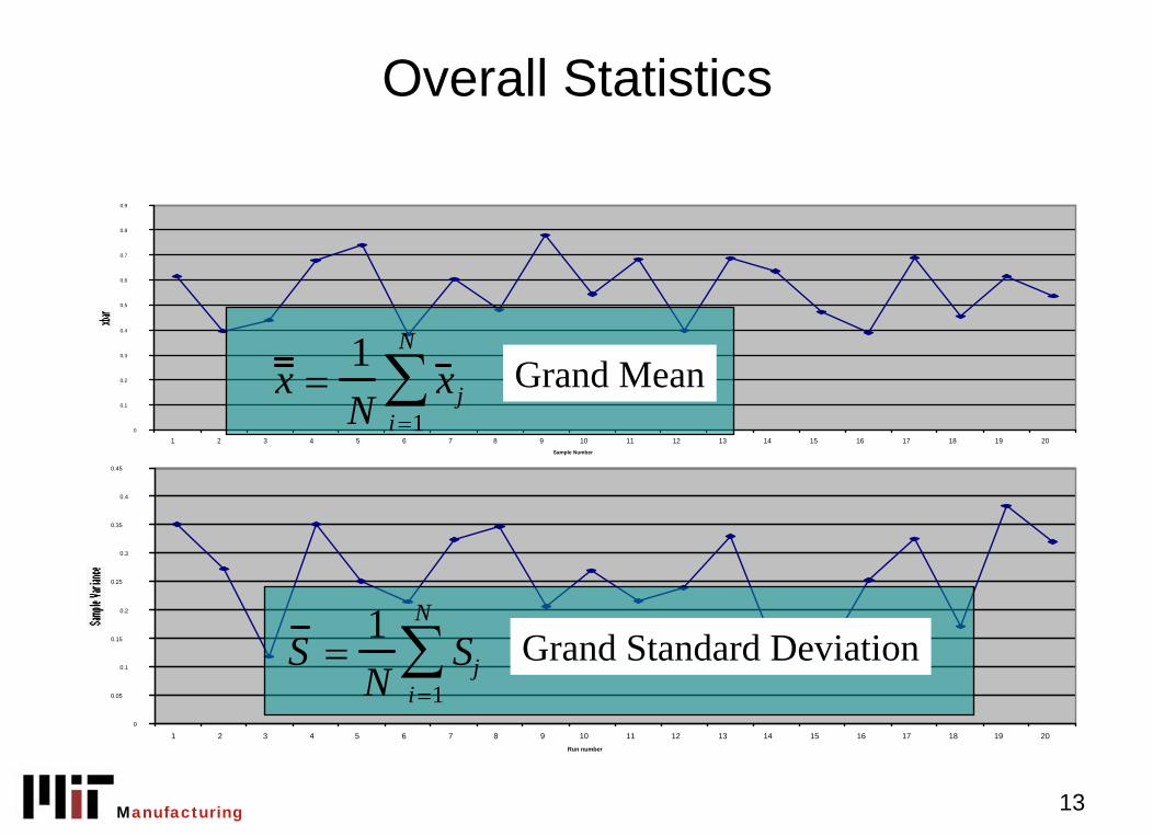
Overall Statistics

0

0.1

0.2

0.3

0.4

0.5

0.6

0.7

0.8

0.9

1 2 3 4 5 6 7 8 9 10 11 12 13 14 15 16 17 18 19 20Sample Number

0

0.05

0.1

0.15

0.2

0.25

0.3

0.35

0.4

0.45

1 2 3 4 5 6 7 8 9 10 11 12 13 14 15 16 17 18 19 20Run number

Grand Meanx =1N

x ji =1

N

∑

S =1N

Sji =1

N

∑ Grand Standard Deviation

14Manufacturing

Setting Chart Limits

• Expected Ranges– Grand mean and Variance

• (based on what data and how many data points?)

• Confidence Intervals– Intervals of + n Standard Deviations– Most Typical is + 3σ (US) or 0.1% (Europe)

15Manufacturing

Chart Limits - Xbar

• If we knew σx then:

• But Since we Estimate the Sample Standard Deviation, then

σ x =1n

σ x

E(Sj) = C4σ x

where C4 =2

n −1⎛ ⎝

⎞ ⎠

1/ 2 Γ(n / 2)Γ((n −1) / 2)

(Sj is a biased estimator)

16Manufacturing

Chart Limits xbar chart

UCL = x + 3S

C4 nLCL = x −3

S C4 n

With this “correction” we can set limit at ±3σxbar

Or set a confidence interval of 99.7%

Or a test significance of 0.3%

For the example n=5 C4 = 0.5( )1/ 2 Γ(2.5)Γ(2)

= 0.7071.33

1= 0.94

17Manufacturing

The variance of the estimate of S can be shown to be:

σS = σ 1 − C42

UCL = S + 3S C4

1 − C42

LCL = S − 3S C4

1 − C42

So we get the chart limits:

Chart Limits S

18Manufacturing

Example xbar

0

0.1

0.2

0.3

0.4

0.5

0.6

0.7

0.8

0.9

1

1 2 3 4 5 6 7 8 9 10 11 12 13 14 15 16 17 18 19 20sample number

UCL

LCL

Grand

Mean

19Manufacturing

Example S

0

0.1

0.2

0.3

0.4

0.5

0.6

0.7

1 2 3 4 5 6 7 8 9 10 11 12 13 14 15 16 17 18 19 20

UCL

LCL

Grand S

20Manufacturing

Detecting Problemsfrom Running Data

• Appearance of data

– Confidence Intervals

– Frequency of extremes

– Trends

21Manufacturing

The 8 rules from Devor et al (Based on Confidence Intervals)

• Prob. of data in a band• Based on Periodicity• Based on Linear Trends• Based on Mean Shift

22Manufacturing

Test for “Out of Control”

• Extreme Points– Outside ±3σ

• Improbable Points– 2 of 3 >±2σ – 4 of 5 >± 1σ– All points inside ±1σ

23Manufacturing

Tests for “Out of Control”• Consistently above or below centerline

– Runs of 8 or more• Linear Trends

– 6 or more points in consistent direction• Bi-Modal Data

– 8 successive points outside ±1σ

24Manufacturing

Applying Shewhart Charting

• Find a run of 25-50 points that are “in-control”• Compute chart centerlines and limits• Begin Plotting subsequent xbarj and Sj

• Apply the 8 rules, or look for trends, improbable events or extremes.

• If these occur, process is “out of control”

25Manufacturing

Out of Control

• Data is not Stationary (μ or σ are not constant)

• Process Output is being “caused” by a disturbance (common cause)

• This disturbance can be identified and eliminated– Trends indicate certain types– Correlation with know events

• shift changes• material changes

26Manufacturing

Western Electric Rules (See Table 4-1)

• Points outside limits• 2-3 consecutive points outside 2 sigma• Four of five consecutive points beyond 1 sigma• Run of 8 consecutive points on one side of

center

27Manufacturing

“In-Control”

i

i+1

i+2

...

What will chart look like?Tim

e

28Manufacturing

“Not In-Control”

i

i+1

i+2

...

Time What will chart

look like?

29Manufacturing

• Consider a real shift of Δμx:

• How many samples before we can expect to detect the shift on the xbar chart?

0

0.1

0.2

0.3

0.4

0.5

0.6

0.7

0.8

0.9

1

1 2 3 4 5 6 7 8 9 10 11 12 13 14 15 16 17 18 19 20Sample Number

Detecting Mean Shifts:Chart Sensitivity

30Manufacturing

• How often will the data exceed the ±3σ limits if Δμx = 0?

Prob(x > μ x + 3σ x ) + Prob(x < μ x − 3σ x )= 3 / 1000

0

0.05

0.1

0.15

0.2

0.25

0.3

0.35

0.4

0.45

-4 -3 -2 -1 0 1 2 3 4μ +3σ−3σ

Average Run Length

31Manufacturing

• How often will the data exceed the ±3σ limits if Δμx = +1σ?

pe

0

0.05

0.1

0.15

0.2

0.25

0.3

0.35

0.4

0.45

-4 -3 -2 -1 0 1 2 3 4

Actual Distribution

Δμ

0

0.05

0.1

0.15

0.2

0.25

0.3

0.35

0.4

0.45

-4 -3 -2 -1 0 1 2 3 4μ +3σ−3σ

Assumed Distribution

Average Run Length

Prob(x > μ x + 2σ x ) + Prob(x < μ x − 4σ x )= 0.023 + 0.001 = 24 / 1000

32Manufacturing

Definition

• Average Run Length (arl): Number of runs (or samples) before we can expect a limit to be exceeded = 1/pe

– for Δμ = 0 arl = 3/1000 = 333 samples– for Δμ = 1σ arl = 24/1000 = 42 samples

Even with a mean shift as large as 1σ, it could take 42 samples before we know it!!!

33Manufacturing

• Assume the same Δμ = 1σ– Note that Δμ is an absolute value

• If we increase n, the Variance of xbar decreases:

• So our ± 3σ limits move closer together

σx =σ x

n

Effect of Sample Size n on ARL

34Manufacturing

0

0.05

0.1

0.15

0.2

0.25

0.3

0.35

0.4

0.45

-4 -3 -2 -1 0 1 2 3 40

0.05

0.1

0.15

0.2

0.25

0.3

0.35

0.4

0.45

-4 -3 -2 -1 0 1 2 3 4

New Distribution

0

0.05

0.1

0.15

0.2

0.25

0.3

0.35

0.4

0.45

-4 -3 -2 -1 0 1 2 3 4μ +3σ−3σ

Original Distribution

ARL Example

pe

+3σ∗−3σ∗new limits

Δμ

same absolute shift

As n increases pe increases so ARL decreases

35Manufacturing

Design of the Chart

• Sample size n– Central Limit theorem– ARL effects?

• Selection of Reference Data– Is S at a minimum ?

• Sample time ΔT– Cost of sampling– production without data– Rapid phenomena

Sample size and “filtering”versus response time to

changes

sample interval ΔT

j j+1j+2 ...

36Manufacturing

Limits and Extensions• Need for averaging• Assumptions of Normality• Assumption of independence• Pitfalls

– Misinterpretation of Data– Improper Sampling

• What are alternatives?– Different Sampling Schemes– Different Averaging Schemes– Continuous Update to Improve Statistics

37Manufacturing

Conclusions

• Hypothesis Testing– Use knowledge of PDFs to evaluate hypotheses– Quantify the degree of certainty (a and b)– Evaluate effect of sampling and sample size

• Shewhart Charts– Application of Statistics to Production– Plot Evolution of Sample Statistics and S– Look for Deviations from Model

x

38Manufacturing

Detection : The SPC Hypothesis

...

...

In-Control

Not

In-Control

0

0.1

0.2

0.3

0.4

0.5

0.6

0.7

0.8

0.9

1 2 3 4 5 6 7 8 9 10 11 12 13 14 15 16 17 18 19 20Sample Number

Process Y

p(y)

39Manufacturing

Out of Control

• Data is not Stationary (μ or σ are not constant)

• Process Output is being “caused” by a disturbance (assignable or special cause)

• This disturbance can be identified and eliminated– Trends indicate certain types– Correlation with know events

• shift changes• material changes

40Manufacturing

Use of the S Chart

• Plot of sample Variance– Variance of the Mean for Shewhart xbar (n>1)

• What Does it Tell Us about State of Control?– It simply plots the “other” statistic

41Manufacturing

Consider this Process Xbar Chart

0

0.1

0.2

0.3

0.4

0.5

0.6

0.7

0.8

0.9

1

1 2 3 4 5 6 7 8 9 10 11 12 13 14 15 16 17 18 19 20

sample number

UCL

LCL

42Manufacturing

And the S Chart

0

0.1

0.2

0.3

0.4

0.5

0.6

1 2 3 4 5 6 7 8 9 10 11 12 13 14 15 16 17 18 19 20

UCL

LCL

43Manufacturing

In Control?

44Manufacturing

Same Process Later in Time

0

0.1

0.2

0.3

0.4

0.5

0.6

0.7

0.8

0.9

1

1 2 3 4 5 6 7 8 9 10 11 12 13 14 15 16 17 18 19 20

sample number

UCL

LCL

Xbar

45Manufacturing

Later S Chart

0

0.1

0.2

0.3

0.4

0.5

0.6

1 2 3 4 5 6 7 8 9 10 11 12 13 14 15 16 17 18 19 20

UCL

LCL

46Manufacturing

What Changed??

47Manufacturing

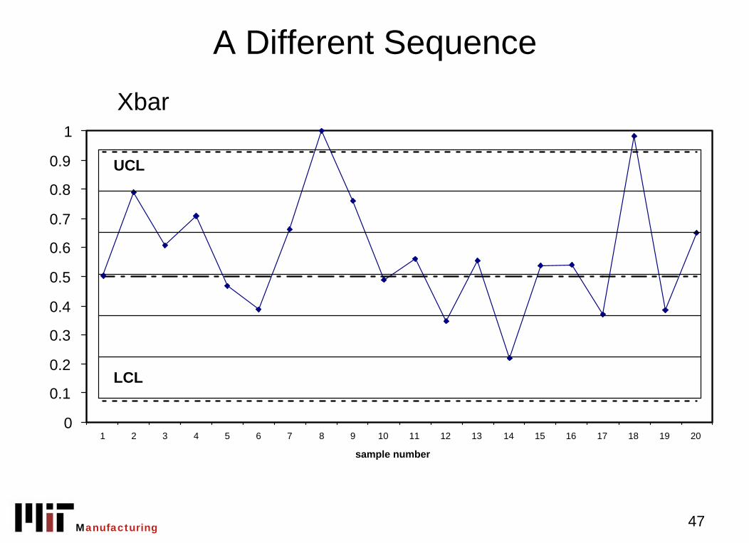
A Different Sequence

0

0.1

0.2

0.3

0.4

0.5

0.6

0.7

0.8

0.9

1

1 2 3 4 5 6 7 8 9 10 11 12 13 14 15 16 17 18 19 20

sample number

UCL

LCL

Xbar

48Manufacturing

S Chart

0

0.1

0.2

0.3

0.4

0.5

0.6

1 2 3 4 5 6 7 8 9 10 11 12 13 14 15 16 17 18 19 20

UCL

LCL

49Manufacturing

Use of S Chart

• Detect Changes in Variance of Parent Distribution

• Distinguish Between Mean and Variance Changes

50Manufacturing

Statistical Process Control

• Model Process as a Normal Independent* Random Variable

• Completely described by μ and σ• Estimate using xbar and s• Enforce Stationary Conditions• Look for Deviations in Either Statistic• If so ………..?• Call an Engineer!

51Manufacturing

Another Use of the Statistical Process Model:

The Manufacturing -Design Interface

• We now have an empirical model of the process

0

0.05

0.1

0.15

0.2

0.25

0.3

0.35

0.4

0.45

-4 -3 -2 -1 0 1 2 3 4

μ +3σ−3σ

How “good” is the process?

Is it capable of producing what we need?

52Manufacturing

Process Capability

• Assume Process is In-control• Described fully by xbar and s• Compare to Design Specifications

– Tolerances– Quality Loss

53Manufacturing

• Tolerances: Upper and Lower Limits

CharacteristicDimension

Targetx*

Upper Specification Limit

USL

Lower Specification Limit

LSL

Design Specifications

54Manufacturing

• Quality Loss: Penalty for Any Deviation from Target

QLF = L*(x-x*)2

Design Specifications

x*=target

How to How to Calibrate?Calibrate?

55Manufacturing

0

0.05

0.1

0.15

0.2

0.25

0.3

0.35

0.4

0.45

-4 -3 -2 -1 0 1 2 3 4μ +3σ−3σx* USLLSL

• Define Process using a Normal Distribution• Superimpose x*, LSL and USL• Evaluate Expected Performance

Use of Tolerances:Process Capability

56Manufacturing

Process Capability

• Definitions

• Compares ranges only• No effect of a mean shift:

Cp =(USL − LSL)

6σ=

tolerance range99.97% confidence range

57Manufacturing

= Minimum of the normalized deviation from the mean

• Compares effect of offsets

Cpk = min(USL − μ)

3σ,(LSL − μ)

3σ⎛ ⎝

⎞ ⎠

Process Capability: Cpk

58Manufacturing

Cp = 1; Cpk = 1

0

0.05

0.1

0.15

0.2

0.25

0.3

0.35

0.4

0.45

-4 -3 -2 -1 0 1 2 3 4

59Manufacturing

Cp = 1; Cpk = 0

0

0.05

0.1

0.15

0.2

0.25

0.3

0.35

0.4

0.45

-4 -3 -2 -1 0 1 2 3 4

60Manufacturing

Cp = 2; Cpk = 1

0

0.05

0.1

0.15

0.2

0.25

0.3

0.35

0.4

0.45

-4 -3 -2 -1 0 1 2 3 4

61Manufacturing

Cp = 2; Cpk = 2

0

0.05

0.1

0.15

0.2

0.25

0.3

0.35

0.4

0.45

-4 -3 -2 -1 0 1 2 3 4

62Manufacturing

Effect of Changes

• In Design Specs• In Process Mean• In Process Variance

• What are good values of Cp and Cpk?

63Manufacturing

Cpk Table

Cpk z P<LS or P>USL

1 3 1E-03

1.33 5 3E-07

1.67 4 3E-05

2 6 1E-09

64Manufacturing

The “6 Sigma” problem

0

0.05

0.1

0.15

0.2

0.25

0.3

0.35

0.4

0.45

-4 -3 -2 -1 0 1 2 3 4

+3σ∗−3σ∗ USLLSL

6σ

P(x > 6σ) = 18.8x10-10 Cp=2

Cpk=2

65Manufacturing

The 6 σ problem: Mean Shifts

0

0.05

0.1

0.15

0.2

0.25

0.3

0.35

0.4

0.45

-4 -3 -2 -1 0 1 2 3 4

USLLSL

4σ

P(x>4σ) = 31.6x10-6 Cp=2

Cpk=4/3Even with a mean shift of 2σwe have only 32 ppm out of spec

66Manufacturing

QLF = L(x) =k*(x-x*)2

Capability from the Quality Loss Function

Given L(x) and p(x) what is E{L(x)}?x*

67Manufacturing

Expected Quality Loss

E{L(x)}= E k(x − x*)2[ ]= k E(x2 ) − 2E(xx*) + E(x *2 )[ ]= kσ x

2 + k(μx − x*)2

Penalizes Variation

Penalizes Deviation

68Manufacturing

Process Capability

• The reality (the process statistics)• The requirements (the design specs)• Cp - a measure of variance vs. tolerance• Cpk - a measure of variance from target• Expected Loss- An overall measure of

goodness