Embed Size (px)
Citation preview

1
MAINLINE
MAINtenance, renewal and Improvement of rail transport iNfrastructure to reduce Economic and environmental impacts
Collaborative project (Small or medium-scale focused research project)
Theme SST.2011.5.2-6.: Cost-effective improvement of rail transport infrastructure
Deliverable 5.7:
Manual for a Life Cycle Assessment Tool (LCAT) for Railway Infrastructure
Metallic Bridges, Track and Soil Cuttings
Grant Agreement number: 285121 SST.2011.5.2-6.
Start date of project: 1 October 2011 Duration: 36 months
Lead beneficiary of this deliverable: Jacobs/SKM
Due date of deliverable: 31/08/2014 Actual submission date: 10/09/2014
Release: Final
Project co-funded by the European Commission within the 7th Framework Programme
Dissemination Level
PU Public X
PP Restricted to other programme participants (including the Commission Services)
RE Restricted to a group specified by the consortium (including the Commission Services)
CO Confidential, only for members of the consortium (including the Commission Services)

D5.7: Usable Tool and Manual MAINLINE SST.2011.5.2-6.
ML-D5.7-Usable_Tool_and_Manual.docx 10/09/2014
PU ©MAINLINE Consortium Page 2
Abstract of the MAINLINE Project
Growth in demand for rail transportation across Europe is predicted to continue. Much of this growth will have to be accommodated on existing lines that contain old infrastructure. This demand will increase both the rate of deterioration of these elderly assets and the need for shorter line closures for maintenance or renewal interventions. The impact of these interventions must be minimized and will also need to take into account the need for lower economic and environmental impacts. New interventions will need to be developed along with additional tools to inform decision makers about the economic and environmental consequences of different intervention options being considered.
MAINLINE proposes to address all these issues through a series of linked work packages that will target at least € 300m per year savings across Europe with a reduced environmental footprint in terms of embodied carbon and other environmental benefits. It will:
Apply new technologies to extend the life of elderly infrastructure Improve degradation and structural models to develop more realistic life cycle cost
and safety models Investigate new construction methods for the replacement of obsolete infrastructure Investigate monitoring techniques to complement or replace existing examination
techniques Develop management tools to assess whole life environmental and economic impact.
The consortium includes leading railways, contractors, consultants and researchers from across Europe, including from both Eastern Europe and the emerging economies. Partners also bring experience on approaches used in other industry sectors which have relevance to the rail sector. Project benefits will come from keeping existing infrastructure in service through the application of technologies and interventions based on life cycle considerations. Although MAINLINE will focus on certain asset types, the management tools developed will be applicable across a broader asset base.
Partners in the MAINLINE Project
UIC, FR; Network Rail Infrastructure Limited, UK; COWI, DK; SKM, UK; University of Surrey, UK; TWI, UK; University of Minho, PT; Luleå tekniska universitet, SE; Deutsche Bahn, DE; MÁV Magyar Államvasutak Zrt, HU; Universitat Politècnica de Catalunya, ES; Graz University of Technology, AT; TCDD, TR; Damill AB, SE; COMSA EMTE, ES; Trafikverket, SE; SETRA, FR; ARTTIC, FR; Skanska a.s., CZ.
WP5 in the MAINLINE project
The main objective of WP5 is to create a tool (Life Cycle Assessment Tool - LCAT) that can compare different maintenance/replacement strategies for track and infrastructure based on a life cycle evaluation.
The evaluation shall quantify:
Direct economic costs Availability (Delay costs/user cost/benefit from upgrade etc.) Environmental impact costs
The comparison cannot be based only in the optimization of the economic and environmental aspects.

D5.7: Usable Tool and Manual MAINLINE SST.2011.5.2-6.
ML-D5.7-Usable_Tool_and_Manual.docx 10/09/2014
PU ©MAINLINE Consortium Page 3
Table of Contents
List of figures .......................................................................................................................6
List of Tables ........................................................................................................................7
Glossary ................................................................................................................................8
1. Executive Summary ......................................................................................................9
2. Acknowledgements ..................................................................................................... 10
3. Introduction ................................................................................................................. 11
3.1 Scope of this report .............................................................................................. 11 3.1.1 Task definition .............................................................................................. 11 3.1.2 Deliverable definition .................................................................................... 11 3.1.3 Significant note ............................................................................................ 11
3.2 Relationship to other Work Packages ................................................................... 12
4. Asset types and sources of data ................................................................................ 13
4.1 Asset Types ......................................................................................................... 13 4.2 Sources of Data ................................................................................................... 14
5. Modelling principles .................................................................................................... 16
5.1 Separation of Asset Types ................................................................................... 16 5.2 Modelling environment ......................................................................................... 16
5.2.1 Technical note .............................................................................................. 16
6. User Interface .............................................................................................................. 17
6.1 Consistency of style ............................................................................................. 17 6.2 Principal features of the models ........................................................................... 17
6.2.1 Groups of worksheets and colour coding ..................................................... 17 6.2.2 Flowchart of data.......................................................................................... 19
7. The Life Cycle Assessment Tool (LCAT) ................................................................... 20
7.1 LCAT inputs ......................................................................................................... 20 7.2 LCAT calculations ................................................................................................ 21 7.3 LCAT outputs ....................................................................................................... 21
8. Soil Cuttings LCAT ...................................................................................................... 23
8.1 Assumptions and modelling techniques ................................................................ 23 8.1.1 The MAINLINE Algorithm for soil cuttings risk assessment .......................... 23 8.1.2 Further assumptions .................................................................................... 24
8.2 Inputs ................................................................................................................... 25 8.2.1 Input of initial asset condition ....................................................................... 25 8.2.2 Input of intervention triggers ......................................................................... 26 8.2.3 Changes caused by interventions (uplift effects) .......................................... 28 8.2.4 Input of intervention costs ............................................................................ 29
8.3 Calculations and inner workings ........................................................................... 33 8.3.1 Initial Scores ................................................................................................ 33 8.3.2 Deterioration Rates ...................................................................................... 33 8.3.3 Projection ..................................................................................................... 33 8.3.4 Results ......................................................................................................... 33

D5.7: Usable Tool and Manual MAINLINE SST.2011.5.2-6.
ML-D5.7-Usable_Tool_and_Manual.docx 10/09/2014
PU ©MAINLINE Consortium Page 4
8.4 Outputs of data ..................................................................................................... 33 8.4.1 Output Summary (Figure 8.7) ....................................................................... 34 8.4.2 Output Financial (Figure 8.8) ........................................................................ 34 8.4.3 Output Environmental (Figure 8.9) ............................................................... 34 8.4.4 Output Operations (Figure 8.10) ................................................................... 34 8.4.5 Output Condition (Figure 8.11) ..................................................................... 34 8.4.6 Summary of outputs ..................................................................................... 40
9. Metallic Bridges LCAT ................................................................................................. 41
9.1 Assumptions and modelling techniques ................................................................ 41 9.1.1 Bridges LCAT application ............................................................................. 41 9.1.2 Deterioration modelling techniques .............................................................. 41 9.1.3 Further assumptions .................................................................................... 46
9.2 Inputs of data ....................................................................................................... 47 9.2.1 Input of initial asset condition ....................................................................... 47 9.2.2 Input of intervention triggers ......................................................................... 49 9.2.3 Changes caused by interventions (uplift effects) .......................................... 52 9.2.4 Input of intervention costs ............................................................................ 52
9.3 Calculations and inner workings ........................................................................... 56 9.3.1 Corrosion Rates ........................................................................................... 56 9.3.2 Element Projection (1) .................................................................................. 56 9.3.3 Results ......................................................................................................... 56
9.4 Outputs of data ..................................................................................................... 56 9.4.1 Output Summary (Figure 9.10) ..................................................................... 56 9.4.2 Output Financial (Figure 9.11) ...................................................................... 57 9.4.3 Output Environmental (Figure 9.12) ............................................................. 57 9.4.4 Output Operations (Figure 9.13) ................................................................... 57 9.4.5 Output Condition (Figure 9.14) ..................................................................... 57 9.4.6 Summary of outputs ..................................................................................... 63
10. Plain Line Track LCAT ............................................................................................ 64
10.1 Assumptions and modelling techniques ............................................................ 64 10.1.1 Deterioration modelling techniques ........................................................ 64 10.1.2 Further assumptions .............................................................................. 65
10.2 Inputs of data .................................................................................................... 66 10.2.1 Input of initial asset condition ................................................................. 66 10.2.2 Input of intervention triggers .................................................................. 67 10.2.3 Changes caused by interventions (uplift effects) .................................... 68 10.2.4 Input of intervention costs ...................................................................... 69
10.3 Calculations and inner workings ........................................................................ 73 10.3.1 Deterioration Rates ................................................................................ 73 10.3.2 Projection .............................................................................................. 73 10.3.3 Results .................................................................................................. 73
10.4 Outputs of data ................................................................................................. 73 10.4.1 Output Summary (Figure 10.8) .............................................................. 73 10.4.2 Output Financial (Figure 10.9) ............................................................... 73 10.4.3 Output Environmental (Figure 10.10) ..................................................... 74 10.4.4 Output Operations (Figure 10.11) .......................................................... 74 10.4.5 Output Condition (Figure 10.12) ............................................................. 74 10.4.6 Summary of outputs ............................................................................... 80 10.4.7 Interpretation of the results .................................................................... 80
11. Limitations of LCATs and Future Work ................................................................. 82

D5.7: Usable Tool and Manual MAINLINE SST.2011.5.2-6.
ML-D5.7-Usable_Tool_and_Manual.docx 10/09/2014
PU ©MAINLINE Consortium Page 5
12. Conclusions ............................................................................................................. 83
13. References ............................................................................................................... 84
14. Appendices .............................................................................................................. 85
14.1 Track LCAT: Performance profiles .................................................................... 85 14.1.1 Performance profile I ............................................................................. 85 14.1.2 Performance profile II ............................................................................ 86 14.1.3 Performance profile III ........................................................................... 87
14.2 VBA Macros for the Bridges LCAT .................................................................... 88 14.2.1 When coating systems data does not exist ............................................ 88 14.2.2 When coating systems data exists ......................................................... 89
14.3 LCAT for Soil Cuttings – Tutorial (Slides from LCAT Training session) ............. 90 14.4 LCAT for Bridges – Tutorial (Slides from LCAT Training session) ................... 103 14.5 LCAT for Track – Tutorial (Slides from the LCAT Training session) ................ 115

D5.7: Usable Tool and Manual MAINLINE SST.2011.5.2-6.
ML-D5.7-Usable_Tool_and_Manual.docx 10/09/2014
PU ©MAINLINE Consortium Page 6
List of figures
Figure 4.1: Track example .................................................................................................... 14 Figure 4.2: Soil cutting example ........................................................................................... 14 Figure 4.3: Metallic bridge example ...................................................................................... 14 Figure 6.1: Colour scheme for Microsoft Excel sheets .......................................................... 17 Figure 6.2: User sheets in LCAT models .............................................................................. 18 Figure 6.3: Data flow chart in LCAT models ......................................................................... 19 Figure 7.1: LCAT inputs ........................................................................................................ 21 Figure 7.2: LCAT calculations............................................................................................... 21 Figure 7.3: LCAT outputs ..................................................................................................... 22 Figure 8.1: Soil Cuttings LCAT- Initial condition .................................................................... 26 Figure 8.2: Soil Cuttings LCAT - Intervention triggers ........................................................... 28 Figure 8.3: Soil Cuttings LCAT - Intervention changes ......................................................... 29 Figure 8.4: Soil Cuttings LCAT - Cost summary sheet .......................................................... 30 Figure 8.5: Soil Cuttings LCAT- Intervention cost details ...................................................... 31 Figure 8.6: Soil Cuttings LCAT - Sample of environmental impact reference data ................ 32 Figure 8.7: Soil Cuttings LCAT - Output summary ............................................................... 35 Figure 8.8: Soil Cuttings LCAT - Financial output ................................................................. 36 Figure 8.9: Soil Cuttings LCAT - Environmental output ......................................................... 37 Figure 8.10: Soil Cuttings LCAT - Operational output ........................................................... 38 Figure 8.11: Soil Cuttings LCAT - Condition output .............................................................. 39 Figure 9.1: Short span metallic bridge .................................................................................. 41 Figure 9.2: Bridge deterioration mechanism ......................................................................... 42 Figure 9.3: Deterioration model for coating system ............................................................... 45 Figure 9.4: Bridges LCAT - Initial condition ........................................................................... 49 Figure 9.5: Bridges LCAT - Condition output ........................................................................ 51 Figure 9.6: Bridges LCAT – Uplift effects .............................................................................. 52 Figure 9.7: Bridges LCAT - Cost summary sheet .................................................................. 53 Figure 9.8: Bridges LCAT - Intervention cost details ............................................................. 54 Figure 9.9: Bridges LCAT - Sample of environmental impact reference data ........................ 55 Figure 9.10: Bridges LCAT - Output summary ..................................................................... 58 Figure 9.11: Bridges LCAT - Financial output ....................................................................... 59 Figure 9.12: Bridges LCAT - Environmental output ............................................................... 60 Figure 9.13: Bridges LCAT - Operational output ................................................................... 61 Figure 9.14: Bridges LCAT - Condition output ...................................................................... 62 Figure 10.1: Track deterioration function .............................................................................. 64 Figure 10.2: Track LCAT – Input parameters ........................................................................ 67 Figure 10.3: Track LCAT - intervention triggers .................................................................... 68 Figure 10.4: Track LCAT - uplift effects ................................................................................ 69 Figure 10.5: Track LCAT - Cost summary sheet ................................................................... 70 Figure 10.6: Track LCAT - Intervention cost details .............................................................. 71 Figure 10.7: Track LCAT - Sample of environmental impact reference data ......................... 72 Figure 10.8: Track LCAT - Output summary ........................................................................ 75 Figure 10.9: Track LCAT - Financial output .......................................................................... 76 Figure 10.10: Track LCAT - Environmental output ................................................................ 77 Figure 10.11: Track LCAT - Operational output .................................................................... 78 Figure 10.12: Track LCAT - Condition output ....................................................................... 79

D5.7: Usable Tool and Manual MAINLINE SST.2011.5.2-6.
ML-D5.7-Usable_Tool_and_Manual.docx 10/09/2014
PU ©MAINLINE Consortium Page 7
List of Tables
Table 8.1: MAINLINE Algorithm factors ................................................................................ 23 Table 8.2: Soil cuttings LCAT assumptions .......................................................................... 24 Table 9.1: Description of atmospheric corrosivity categories and corresponding corrosion
rates (MAILINE, 2013) .......................................................................................................... 43 Table 9.2: Exposure conditions assumed for bridge Elements.............................................. 44 Table 9.3: Description and expected service life of protective coatings (ML D2.3) ................ 44 Table 9.4: Parameters assumed for exposure conditions of bridge Elements. ...................... 46 Table 9.5: Bridges LCAT assumptions ................................................................................. 47 Table 10.1: Track LCAT assumptions ................................................................................... 66

D5.7: Usable Tool and Manual MAINLINE SST.2011.5.2-6.
ML-D5.7-Usable_Tool_and_Manual.docx 10/09/2014
PU ©MAINLINE Consortium Page 8
Glossary
Abbreviation/ acronym
Description
BA Burrowing Assessment
CAA Construction Activity Assessment
DA Drainage Assessment
LCA Life Cycle Analysis
LCAT Life Cycle Assessment Tool
LCC Life Cycle Cost
MA Movement Assessment
ML Mainline Project
MS Excel Microsoft Excel
NR Network Rail Infrastructure Limited [Great Britain Infrastructure Manager]
O&M Operations & Maintenance
OeBB Austrian Federal Railways [Austrian Infrastructure Manager]
SRV Slope Risk Value
SSHI Soil Slope Hazard Index
SWA Surface Water Assessment
VA Vegetation Assessment
VBA Visual Basic Application
WP Work Package

D5.7: Usable Tool and Manual MAINLINE SST.2011.5.2-6.
ML-D5.7-Usable_Tool_and_Manual.docx 10/09/2014
PU ©MAINLINE Consortium Page 9
1. Executive Summary
This report accompanies the final release of Life-Cycle Assessment Tools (LCATs) for Metallic Bridges, Plain Track and Soil Cuttings as Phase 3 of Task 5.5 of the MAINLINE project and includes the demonstration of these models with extensive information and guidance on how to use them.
The Life-Cycle Assessment Tools have been developed using the data and information made available to the project team. From the research completed in other MAINLINE Work Packages, it is clear that the LCAT models presented here improve on previous modelling practice in two key areas, in that they:
- incorporate mechanisms to estimate deterioration of assets - assess the environmental impact of interventions alongside their financial and
operational impacts.
The method of modelling within each of these LCATs is innovative, detailed and they have been individually developed based on the specific engineering characteristics of the asset types.
The models are provided as Microsoft Excel workbooks for each asset type. This is a medium widely used by partners in the MAINLINE project and in the industry in general. The models are extensively annotated with all the calculations explicitly shown and do not include any obscure programming code. This is intended to allow the workings of the models to be examined and reviewed by other partners and keep the models as transparent as possible.
The Life-Cycle Assessment Tools are prototypes; they are meant to prove a concept. Also, their final release was accompanied by two open training seminars in London and Paris to spread the knowledge and inform the rail community about these developments.
Disclaimer:
The authors of this report (incl. developed LCATs) have used their best endeavours to ensure that the information presented here is of the highest quality. However, no liability can be accepted by the authors for any loss caused by its use.

D5.7: Usable Tool and Manual MAINLINE SST.2011.5.2-6.
ML-D5.7-Usable_Tool_and_Manual.docx 10/09/2014
PU ©MAINLINE Consortium Page 10
2. Acknowledgements
This report has been prepared within Work Package 5 of the MAINLINE project by the following team of contractors, with Jacobs/SKM acting as the deliverable co-ordinator and Network Rail acting as WP leader:
NR Network Rail Infrastructure Limited UK
COWI COWI Denmark
Jacobs/SKM Jacobs/Sinclair Knight Merz UK
Surrey University of Surrey UK
UMINHO University of Minho Portugal
LTU Luleå University of Technology Sweden
TUGraz Graz University of Technology Austria
TCDD Turkish State Railways (Türkiye Cumhuriyeti Devlet Demiryolları) Turkey
Discussions with and feedback from all MAINLINE partners are gratefully acknowledged. Also, particular thanks are due to the Internal Reviewers and the members of the Project Advisory Committee who have undertaken the technical review of the present deliverable.

D5.7: Usable Tool and Manual MAINLINE SST.2011.5.2-6.
ML-D5.7-Usable_Tool_and_Manual.docx 10/09/2014
PU ©MAINLINE Consortium Page 11
3. Introduction
3.1 Scope of this report
This Deliverable D5.7 derives from phase 3 of Task 5.5 within Work Package 5 of the MAINLINE project.
3.1.1 Task definition
Task 5.5 is described in the MAINLINE Description of Work (page 20) as:
“Task 5.5: Development of MAINLINE LCAT (M16-M36), Jacobs/SKM, Surrey, TCDD, COWI, UMINHO, LTU, TUGRAZ, UIC
The tool will be designed to bring together in a quantified manner, the economic and environmental consideration required to inform management decision makers on the selection of the optimum approach. This work will be undertaken in three distinct phases, outlined below, which reflect the exchange of intermediate deliverables with Task 5.6:
- Phase 1: (M16 to 27), Develop a prototype of the LCAT having limited functionality and pass to WP5.6 to test and validate.
- Phase 2: (M28 to 32), Continue to add functionality to prototype LCAT
- Phase 3: (M33 to 36), Finalise LCAT in the light of the testing and validation carried out in Task 5.6, write user manual, apply for patent protection (if necessary), prepare material for final workshop”
3.1.2 Deliverable definition
Deliverable 5.7 is described in the MAINLINE Description of Work (page 21) as:
“D5.7) Usable tool and manual: This deliverable will report the activities of phase 3 of Task 5.5 and will consist of the final version of the proposed LCAT. This version will not be a fully functioning piece of software, rather it will consist of recommendations and algorithms for inclusion in existing software by those who already have tools in use, or which can be used by commercial software houses to develop a commercial product for sale. [month 35]”.
3.1.3 Significant note
It is worthwhile to stress that the user should be aware that these tools are prototypes; they are meant to quantify the whole life cycle evaluation concept and prove that sophisticated decision support tools can be applied to the asset management of railway infrastructure. Nevertheless, they are not intended to capture all the features of asset management methodologies.
Different users may have particular requirements for the models and rail infrastructure managers may use unique strategies or have access to bespoke data. These issues can be addressed in future projects with further customisation of the product required to meet the specific needs of a user.

D5.7: Usable Tool and Manual MAINLINE SST.2011.5.2-6.
ML-D5.7-Usable_Tool_and_Manual.docx 10/09/2014
PU ©MAINLINE Consortium Page 12
3.2 Relationship to other Work Packages
The user manual is based on the development of the Life Cycle Assessment Tools (LCATs) in Task 5.5 and the modelling concepts identified in the report D5.4 (Methodology) which was in turn informed by the work completed in Tasks 5.1 (Current practice), 5.2 (Environmental assessment) and 5.3 (Current tools).
The deterioration data used in the models was derived in WP2 and future collection of such data can be enhanced by the methods identified in WP4 (monitoring). The interventions used in the models are informed by the concepts developed in WP1 (extension of asset life) and WP3 (new construction methods).
Therefore, this document should be read in conjunction with the following previous deliverables from the MAINLINE project:
ML D2.1 Degradation and performance specification for selected assets
ML D2.2 Degradation and intervention modelling techniques
ML D2.3 Time-variant performance profiles for LCC and LCA
ML D2.4 Field validation of performance profiles
ML D5.2 Assessment of environmental performance tools and methods
ML D5.6 Verification report of LCAT models
Additionally, this report is accompanied with the three developed LCAT models:
Soil Cuttings LCAT – [ML_D5 5_SoilCuttingsModel_v06 00.xlsm]
Bridges LCAT – [ML_D5 5_MetallicBridgesModel_v09 00.xlsm]
Track LCAT – [ML_D5 5_PlainTrackModel_v11 00.xlsm]

D5.7: Usable Tool and Manual MAINLINE SST.2011.5.2-6.
ML-D5.7-Usable_Tool_and_Manual.docx 10/09/2014
PU ©MAINLINE Consortium Page 13
4. Asset types and sources of data
4.1 Asset Types
In report ML D2.1 (MAINLINE, 2012), Section 1.5 suggests the types of assets to be modelled:
“The following asset types are identified as focus areas due to the high probability for knowledge increase within the next 3 year period and with useful validation data being available:
Cuttings Metallic bridges Tunnels with concrete and masonry linings Plain track (total track superstructure) and switches and crossings Retaining walls”
Despite the best efforts of the MAINLINE partners, the required data for ML D2.3 (MAINLINE, 2013), has not been forthcoming for all of these asset types, which has prevented the development of deterioration profiles for a number of asset types.
In the case of Rock Cuttings, Switches & Crossings and Retaining Walls, research from the MAINLINE partners in WP2 concluded that no source of data or adequate theory to support the deterioration modelling could be found by the project team and therefore deterioration models for these types of assets could not be developed.
In the case of Lined Tunnels, some theoretical concepts on the deterioration of concrete linings have been found (MAILINE, 2013), however these were not sufficient to support the development of a model for concrete-lined Tunnels. In particular, only a very small proportion of the phenomena associated with the lifecycle modelling of tunnels have been quantified in WP2:
Only a single performance profile has been quantified to date
The methodology and content included in ML D2.3 (MAILINE, 2013), is not specific to
concrete tunnels; it is about reinforced concrete generally
Intervention uplift effects are not quantified
It was decided amongst the MAINLINE partners that due to lack of sufficient data, an LCAT for tunnels could not be devised.
Hence LCATs have been developed for Metallic Bridges, Soil Cuttings and Plain Line Track under Task 5.5 of WP5. These asset types represent a good variety of structural, track and geotechnical asset types. The method of modelling within each of these LCATs is bespoke, detailed and the tools have been individually custom-designed based on the individual engineering behaviour of the asset types.
Typical examples of these assets are illustrated in the pictures below:

D5.7: Usable Tool and Manual MAINLINE SST.2011.5.2-6.
ML-D5.7-Usable_Tool_and_Manual.docx 10/09/2014
PU ©MAINLINE Consortium Page 14
4.2 Sources of Data
The development of successful LCAT models depends on the foundation of deterioration modelling techniques, establishment of deterioration rates and intervention strategies appropriate for each asset type and component.
In the case of soil cuttings, historical data from Network Rail (NR) in the UK was used to derive the deterioration profiles in ML D2.3 (MAILINE, 2013). This is the only known available source of extensive, numerical, and historical data regarding the condition of soil cuttings from which trends have been derived. The NR soil cutting scoring system is known as the Soil Slope Hazard Index (SSHI) and the data includes details of the location and date of each examination but also crucially describes the critical features and condition of the soil slopes in terms of predefined characteristics with alpha-numeric scores.
Figure 4.2: Soil cutting example Figure 4.1: Track example
Figure 4.3: Metallic bridge example

D5.7: Usable Tool and Manual MAINLINE SST.2011.5.2-6.
ML-D5.7-Usable_Tool_and_Manual.docx 10/09/2014
PU ©MAINLINE Consortium Page 15
Likewise in the case of plain line track, extensive data on track performance from the Austrian, Swiss, Croatian, and Norwegian Railway Networks has been collected and analysed under ML D2.3 (MAILINE, 2013). Finally, in the case of metallic bridges, theoretical rates of coating loss and steel corrosion have been developed to provide rates of deterioration of individual steel members and, by implication, an indication of the overall bridge condition.

D5.7: Usable Tool and Manual MAINLINE SST.2011.5.2-6.
ML-D5.7-Usable_Tool_and_Manual.docx 10/09/2014
PU ©MAINLINE Consortium Page 16
5. Modelling principles
5.1 Separation of Asset Types
In the interests of clarity and simplicity, the models for each asset type are independent. There is therefore a separate Microsoft Excel file for each asset type (i.e. Metallic Bridges, Soil Cuttings and Plain Track).
In the future, the models might be developed as a commercial product in which the principles from the separate LCAT models could be combined to allow the user to process various asset types together and thereby to assess work on multiple assets on a section of railway.
5.2 Modelling environment
As mentioned above, the LCAT models have all been developed in Microsoft Excel. This was chosen as a generally acceptable, easily available and accessible application which allows the models to be transferred between MAINLINE partners for review and discussion, and ultimately used by asset managers across Europe and beyond. The model files are typically around 1 MB in size.
All the calculations in the models have mainly been carried out by spreadsheet formulae. Apart from a short section in the Bridges LCAT model, macros and VBA programming have deliberately been avoided. This is intended to allow all stakeholders to see and appreciate the operations of the models, and to update them as appropriate for their particular circumstances.
Continuing on the theme of transparency, all the rows, columns and sheets in the models are visible to the user. However, the user should be mindful that most of the cells are not intended for data input and under other circumstances they would have been locked (protected).
5.2.1 Technical note
The Microsoft Excel version used for the models is 14.0.7106.5003, which is part of Microsoft Office 2010.
The files are stored in ‘macro’ format, which is as .xlsm files. This is necessary because the models include some on-screen input buttons and in some cases, limited application of VBA coding and macros.

D5.7: Usable Tool and Manual MAINLINE SST.2011.5.2-6.
ML-D5.7-Usable_Tool_and_Manual.docx 10/09/2014
PU ©MAINLINE Consortium Page 17
6. User Interface
6.1 Consistency of style
Despite building the models in separate Microsoft Excel files, every effort has been made to make the user interfaces as consistent as possible. The range of worksheets within each model is as similar as possible and the layout and colour scheme of the principal worksheets has been standardised. Navigation within the models is also standardised with hyperlinks between key worksheets.
The different asset types clearly require different calculation techniques and deterioration mechanisms but this is not evident in the main user input and output worksheets.
Within each model, including in the more complex inner workings, extensive notes, comments and data validation is used to help the user and the reviewer to understand and thoroughly appreciate what the model does.
6.2 Principal features of the models
The principal features of the models are outlined in the following sections with example screen-shots of the worksheets within each model. All the information given below is conveniently included in the notes and comments built into the models. It is shown here for clarity.
6.2.1 Groups of worksheets and colour coding
The worksheets within each Microsoft Excel model are colour-coded and grouped to help the user to navigate within the models. The groups are colour-coded as follows:
Sheet colours:
NOTES Black tab sheets are general instructions and information about the model
INPUT Blue tab sheets are for data input
OUTPUT Purple tabs are output sheets
INTV COST Green tabs are sheets for the user to calculate costs and environmental impacts of interventions
ENV REFS Yellow tab is a sheet of environmental reference data
CALCULATION Red tabs are calculation sheets, which the user can see but does not need to change
Figure 6.1: Colour scheme for Microsoft Excel sheets
The calculation sheets include the core workings of the models but are not necessarily of interest to the typical user. However, these worksheets are available to be inspected so that

D5.7: Usable Tool and Manual MAINLINE SST.2011.5.2-6.
ML-D5.7-Usable_Tool_and_Manual.docx 10/09/2014
PU ©MAINLINE Consortium Page 18
the deterioration mechanisms and the modelling principles of the models can be fully appreciated.
The worksheets of particular interest to the typical user are as follows:
Information: Introduction
Brief introduction to the MAINLINE project.
Bridges/Track/CuttingsLCAT Brief introduction to the particular LCAT model.
Flowchart
Outline of data flow in the model, with dynamic links to sheets
Instructions The sheet of instructions
TechNotes Some technical details about the LCAT model
User inputs: InputCondition Select the conditions which best describe the asset and its
initial condition
IntvTriggers This lists the interventions which may be used and their triggering mechanisms; additional interventions may be added.
IntvChanges This sheet shows the ways in which the condition changes after the interventions (uplift effects)
IntvCosts Enter the costs and environmental impacts of each intervention
IntvCost (1)-(15) Build-up of costs and impacts for each intervention; there are 10 sheets, one for each intervention
EnvImpacts Reference list of impacts of construction material and operations
User outputs:
Summary Insert reference and title of modelling run. This shows a summary of the modelling results.
OutputFinancial This shows a summary of the projected financial costs
OutputEnv This shows a summary of the projected environmental impacts
OutputOps
This shows a summary of the projected operational impacts
OutputCondition This shows a summary of the projected condition
Figure 6.2: User sheets in LCAT models
Input data cells:

D5.7: Usable Tool and Manual MAINLINE SST.2011.5.2-6.
ML-D5.7-Usable_Tool_and_Manual.docx 10/09/2014
PU ©MAINLINE Consortium Page 19
Throughout the model the cells coloured light blue are available for user input. To prevent accidental alteration of essential formulae, the user is encouraged not to attempt to modify any cells/sheets with a different colour.
6.2.2 Flowchart of data
The worksheet normally displayed when the model is first opened is the flow chart, shown below:
Figure 6.3: Data flow chart in LCAT models
The main features of this flowchart have been kept the same in all the LCAT models, to maximize consistency and for ease of use.
The flowchart illustrates the relationships and the inter-correlation between the different worksheets of the LCAT model. It demonstrates the process of the algorithm from user input sheets (blue colour), to the intermediate calculations and modelling techniques sheets (red colour) and finally to the results sheets (purple colour).
The user may click on any box-heading to go to that part of the model. The user may move between sheets using the standard functionality of Microsoft Excel.

D5.7: Usable Tool and Manual MAINLINE SST.2011.5.2-6.
ML-D5.7-Usable_Tool_and_Manual.docx 10/09/2014
PU ©MAINLINE Consortium Page 20
7. The Life Cycle Assessment Tool (LCAT)
Each LCAT is a forecasting tool that compares different maintenance and intervention strategies for the selected asset based on a life cycle evaluation. A Life-Cycle Assessment is ‘the comparison and evaluation of the inputs/outputs and the potential environmental impacts of a system during its lifetime (ISO 14040, 2006). Such a lifecycle evaluation attempts to quantify and model:
- Direct economic costs - Availability (delay costs / user cost) - Environmental impact costs
With this in mind, the LCAT is a decision support tool that tries to quantify the costs (financial, operational and environmental) and the risks associated with different intervention strategies. Stated differently, it attempts to model the real life behaviour of rail infrastructure assets in order to usefully predict demands, service life and costs in the future over a period of 100 years.
Like all mathematical models, the LCAT features:
- Inputs - Calculations - Outputs
7.1 LCAT inputs
The user inputs for all models are shown below:
- Asset starting condition - Operating environment - Intervention rules - Uplifts due to intervention - Intervention characteristics:
Costs
Operational impacts
Environmental impacts

D5.7: Usable Tool and Manual MAINLINE SST.2011.5.2-6.
ML-D5.7-Usable_Tool_and_Manual.docx 10/09/2014
PU ©MAINLINE Consortium Page 21
Figure 7.1: LCAT inputs
7.2 LCAT calculations
Once the user has specified the inputs, the LCAT proceeds with the pre-programmed internal calculations. This comprises the core function of the tool and compares all the pre-defined triggers by the user intervention strategies (based on their corresponding triggers) against the current condition of the asset, estimating financial and environmental costs over time.
These calculations employ deterministic, time-stepped modelling methodologies and are subject-specific for each asset type.
Figure 7.2: LCAT calculations
7.3 LCAT outputs
- In the last step, the results of the LCAT are presented in five individual worksheets. The outputs are both graphical and tabular and the user can select which outputs they would like to review. The intervention plan can be expressed in different formats as follows : Cost of interventions over time (also discounted Net Present value [NPV])
- Environmental impacts of interventions over time - Operational impacts of interventions over time

D5.7: Usable Tool and Manual MAINLINE SST.2011.5.2-6.
ML-D5.7-Usable_Tool_and_Manual.docx 10/09/2014
PU ©MAINLINE Consortium Page 22
- Condition of the asset over time
Figure 7.3: LCAT outputs
To summarise, the LCAT prototypes are intended to provide elements of Life Cycle Analysis (LCA) and Life Cycle Cost (LCC) in one model and they are developed to help rail infrastructure managers to:
- Justify work based on evidence - Spend the maintenance budget efficiently - Define and monitor levels of safety and service - Predict timing of future expenditure - Provide consistency between different users

D5.7: Usable Tool and Manual MAINLINE SST.2011.5.2-6.
ML-D5.7-Usable_Tool_and_Manual.docx 10/09/2014
PU ©MAINLINE Consortium Page 23
8. Soil Cuttings LCAT
8.1 Assumptions and modelling techniques
8.1.1 The MAINLINE Algorithm for soil cuttings risk assessment
The Soil Cuttings LCAT is a decision tool that compares different maintenance and intervention strategies for soil cuttings based on a life cycle evaluation and attempts to quantify the costs and risks associated with such strategies over a period of one hundred years.
Soil cuttings are man-made slopes through natural ground; they typically consist of the naturally occurring strata at that location. For that reason, their engineering properties and deterioration mechanisms depend on the soil type which is highly variable across different regions and countries (MAINLINE, 2013). These highly variable soil properties lead to high uncertainty regarding deterioration and performance of this asset.
Therefore, a risk based approach that takes into account multiple possible deterioration mechanisms needs to be adopted in order to assess a cutting’s condition (MAINLINE, 2013). With this in mind, the Network Rail (NR) condition assessment system for soil cuttings was reviewed and a comprehensive data analysis exercise was undertaken, to translate Network Rail’s soil cuttings assessment methodology (known as SSHI) into a more generalised tool (known as MAINLINE Algorithm) that processes data and calculates the current condition of a soil cutting (MAINLINE, 2013).
This tool was designed to be readily adapted to suit different regions within Europe and the sub-scores assigned to each factor are based on the presence of various features in the cutting. The full list of variables is given below:
Table 8.1: MAINLINE Algorithm factors
Group Score Characteristic measured
Permanent
ST Soil Type: Granular, Cohesive or Inter-bedded
SHF Slope Height Factor: height and angle
ALF Adjacent Land Factor: slope and drainage of adjacent land
Variable
MA Movement Assessment: heave or bulge on slope or toe
VA Vegetation Assessment: extent of trees and grass
SW Surface Water Assessment: extent of surface water
DA Drainage Assessment: condition of drains, if any
BA Burrowing Assessment: extent of animal burrowing
CA Construction Activity Assessment: presence of construction work

D5.7: Usable Tool and Manual MAINLINE SST.2011.5.2-6.
ML-D5.7-Usable_Tool_and_Manual.docx 10/09/2014
PU ©MAINLINE Consortium Page 24
The MAINLINE Algorithm factors can be divided into two parts: those which are assumed to be essentially permanent over the life of the LCAT model (e.g. soil type and overall geometry) and those features which may vary (e.g. drainage and vegetation).
These sub-scores are combined to give an overall Slope Risk Value (SRV) which typically varied between 0 and 20, the higher values indicating more risk. For more detailed information the user is advised to read the soil cuttings section of ML D2.2 (MAINLINE, 2012b), D2.3 (MAILINE, 2013) and D2.4 (MAINLINE, 2014a).
Last but not least, historical data from Network Rail (NR) in the UK was used to derive the deterministic deterioration profiles used in the Soil Cuttings LCAT (MAILINE, 2013).
8.1.2 Further assumptions
The Soil Cuttings LCAT does not have a length dimension. It can accommodate any length; the user may specify the appropriate length based on relevant cost information. With respect to the selected deterioration modelling technique, this was chosen to be deterministic and the reasoning is explained in more detail in the ML D2.3 (MAILINE, 2013) and D2.4 (MAILINE, 2014a).
In terms of the modelled interventions, the tool is fully flexible. It can quantify any intervention that rail infrastructure managers might use. There are up to 15 different interventions that can be defined; the default version of the model contains 7 pre-programmed interventions but these can be changed by the user.
The table below summarises the parameters of the LCAT.
Table 8.2: Soil cuttings LCAT assumptions
LCAT model Modelled element
Modelled parameters
Modelling approach
Interventions Time step
Soil Cuttings A length of
Cutting
Generalised Risk Score (MAINLINE Algorithm)
Deterministic
Any - up to 15 types (can be
defined by the user)
5 yearly
The next pages of the soil cuttings LCAT section are intended to walk the user through the algorithmic process of the ‘inputs-calculations-outputs’ that the tool employs and demonstrate how the tool actually works by presenting typical screenshots.
For a tutorial of the model using real case studies, the user is encouraged to read the Appendix 14.3, which contains the slides form the demonstration of the LCAT in the MAINLINE training sessions and the ML D5.6 (MAILINE, 2014b).

D5.7: Usable Tool and Manual MAINLINE SST.2011.5.2-6.
ML-D5.7-Usable_Tool_and_Manual.docx 10/09/2014
PU ©MAINLINE Consortium Page 25
8.2 Inputs
The Soil Cuttings LCAT requires four different input categories. As mentioned earlier, only blue colour cells require data entry.
- Initial asset condition - Intervention triggers - Uplift effects - Costs of interventions and environmental impacts
8.2.1 Input of initial asset condition
The first data requirement is the condition of the underlying soil cutting at the start of the model run.
The model requires the user to undertake either a site inspection or desk study to determine the starting condition of the asset based on a set of standardised questions. This set of standardised questions comprises a form that should ideally be filled in by a geotechnical engineer. A typical example can be seen in the figure below.

D5.7: Usable Tool and Manual MAINLINE SST.2011.5.2-6.
ML-D5.7-Usable_Tool_and_Manual.docx 10/09/2014
PU ©MAINLINE Consortium Page 26
Figure 8.1: Soil Cuttings LCAT- Initial condition
This data is translated into key scores for the soil cuttings in the MAINLINE Algorithm system.
8.2.2 Input of intervention triggers
Interventions are listed on this worksheet and the user may adjust the MAINLINE Algorithm scores at which interventions may be triggered. There are a number of pre-set interventions built into the model but the user may add/delete/adjust interventions, if required. It is recommended that users may create definitions for the conditions that relate to the upper and lower bound figures. This will help consistency educate users on real examples to bring context to the LCAT.
Each intervention may be initiated by any score value (ranging between min-max limits) and these ‘trigger scores’ are entered on this worksheet (in blue cells). Alternatively, the user may

D5.7: Usable Tool and Manual MAINLINE SST.2011.5.2-6.
ML-D5.7-Usable_Tool_and_Manual.docx 10/09/2014
PU ©MAINLINE Consortium Page 27
specify times when the interventions are to be used (i.e. for example intervention No.1 should be applied every ten years).
The sequence in which the scores are tested for triggering an intervention is specified in the column headed ‘Seq’. This ensures that if, for example, a major intervention is applied then minor works will not also be applied in the same period.
In the Soil Cuttings model, below, there are 7 pre-set interventions. These are triggered variously by score values and user-specified timings and are as follows:
Major earthworks intervention (it can be any major intervention)
Minor earthworks intervention (it can be any minor intervention)
Burrow filling
Drainage replacement
Drainage repair
Drainage clearance
Vegetation clearance
For more information about soil cuttings interventions and how they affect the MAINLINE Algorithm and the overall slope risk score (SRV), the user is advised to read ML D2.2 (MAILINE, 2012b).

D5.7: Usable Tool and Manual MAINLINE SST.2011.5.2-6.
ML-D5.7-Usable_Tool_and_Manual.docx 10/09/2014
PU ©MAINLINE Consortium Page 28
Figure 8.2: Soil Cuttings LCAT - Intervention triggers
8.2.3 Changes caused by interventions (uplift effects)
Interventions are applied to the asset in order to change its condition, improving its MAINLINE Algorithm sub-scores as well as the final Slope Risk Value (SRV) score. The model allows the user to input the changes in scores which each intervention is expected to achieve (uplift effects after intervention).
These are specified as either ‘relative’ or ‘absolute’ changes. Relative changes mean that the score will be changed by the addition of the specified amount (uplift) to the pre-existing MAINLINE Algorithm score. Absolute changes set the score to the specified value irrespective of the pre-existing MAINLINE Algorithm score. The example below from the soil cuttings model shows some examples of both types of score change.
It should be noted an intervention may change several MAINLINE Algorithm sub-scores, as shown below where ‘Major earthworks’ has an influence on improving all the condition scores, whereas ‘Drainage repair’ only changes the ‘Drainage Assessment’ score (DA).

D5.7: Usable Tool and Manual MAINLINE SST.2011.5.2-6.
ML-D5.7-Usable_Tool_and_Manual.docx 10/09/2014
PU ©MAINLINE Consortium Page 29
Figure 8.3: Soil Cuttings LCAT - Intervention changes
8.2.4 Input of intervention costs
The costs and impacts of each intervention are summarised on the Intervention Costs worksheet below (‘IntvCosts’ – Figure 8.4), but details of the costs and environmental impacts are input on a separate, more detailed worksheet for each of the fifteen interventions called ‘IntvCost(i)’.
On the cost summary sheet the user may specify cost categories and budgets which may be chosen to suit the user’s own financial arrangements.
Also on the cost summary worksheet the user may identify some operational (e.g. possession costs) and environmental impacts which will arise when the intervention is executed. These may be selected by the user. An operational or environmental impact may include a cash cost which is input here as the cash equivalent of the operational/environmental impact (as kg of CO2 emissions). The discount rates are input on

D5.7: Usable Tool and Manual MAINLINE SST.2011.5.2-6.
ML-D5.7-Usable_Tool_and_Manual.docx 10/09/2014
PU ©MAINLINE Consortium Page 30
the cost summary. Different rates may be specified for cash costs and environmental equivalent costs. The selection of rates is at the discretion of the user.
The example below illustrates sample input figures for Intervention Costs.
Figure 8.4: Soil Cuttings LCAT - Cost summary sheet

D5.7: Usable Tool and Manual MAINLINE SST.2011.5.2-6.
ML-D5.7-Usable_Tool_and_Manual.docx 10/09/2014
PU ©MAINLINE Consortium Page 31
The detailed costs and environmental impact for each intervention is shown in individual costing sheets, as below:
Figure 8.5: Soil Cuttings LCAT- Intervention cost details
The user may specify detailed financial costs associated with the particular intervention, split into different categories (i.e. Labour, Plant, Materials, Tax) as well as greenhouse gases emission, measured by their carbon dioxide equivalent mass (kg CO2e) unit. It is worthwhile to mention that the environmental impacts can be measured by three different environmental effects. Carbon emission (CO2 greenhouse gases emission) is the first pre-set environmental measure, however, the user may specify up to three different ones (i.e. waste, water pollution etc.). For example, the ML D5.2 (MAILINE, 2012c) pointed out that the next most relevant impacts after the greenhouse gases emission is waste. The sum of these CO2 emissions is translated into cash using the user’s pre-set cash equivalent factor.
MAINLINE Soil Cutting Model
Costs & Environment Impact of Intervention
Enter costs and environmental impacts for this intervention
Interv. No: 4
Intervention: Drainage replacement
Scale: ONE intervention treats: 200 m
Item Labour Plant Materials Tax TOTAL Environmental Impact UsageUnit of
usage
Carbon
Dioxide
equivalent
Notes on estimation
€ € € € € kg (CO2e)
Excavation € 2,000 € 2,000 Excavator (5) t 0.550
Road transport € 1,000 € 1,000 Road transport EURO3 (5) t-km 0.022
Manpower € 2,000 € 2,000 - -
GRP drainage pipe € 2,000 € 2,000 GRP drainage pipe 200.00 m 86.519
Concrete in-fill € 20 € 20 Concrete, mass insitu 5.00 m3 221.260
Precast units € 200 € 200 Concrete, precast 5.00 m3 333.600
€ 0 - -
€ 0 - -
€ 0 - -
€ 0 - -
€ 0 - -
€ 0 - -
€ 0 - -
€ 0 - -
€ 0 - -
€ 0 - -
User defined impacts
€ 0
€ 0
Totals € 2,000 € 3,000 € 2,220 € 0 € 7,220 Carried to 'IntvCosts' 20,078 Carried to 'IntvCosts'
Financial Costs Estimate [Euros] Environamental Impact Assessment
back to: Flowchart

D5.7: Usable Tool and Manual MAINLINE SST.2011.5.2-6.
ML-D5.7-Usable_Tool_and_Manual.docx 10/09/2014
PU ©MAINLINE Consortium Page 32
Assessment of environmental impacts
The environmental impact of each item on the cost details sheet is drawn from a reference list of impacts which is common to all models and all interventions.
This library of environmental impacts is a result of a detailed environmental analysis undertaken as part of the MAINLINE project and includes state of the art research (for more information, the user is advised to read the ML D5.2 (MAILINE, 2012c) which focuses on this research). This library may be used to build up the environmental impacts for any intervention. The user has the choice to add further environmental impacts according to their standards and conditions.
A sample from the reference list is given below:
Figure 8.6: Soil Cuttings LCAT - Sample of environmental impact reference data
MAINLINE Soil Cutting Model
Environment Impact of Construction Activity
version 3
Users may amend this data and add more data if necessary
NOTES:
1 These impact values will be used to build-up the environmental impact of the interventions employed in asset life-cycles.
2 The data will be applicable across Europe. If it is specific to a certain country, this is noted.
3 The impacts of materials are shown as from cradle-to-factorygate.
4 The impacts of equipment and transport will include only fuel usage (excluding the manufacture of the equipment or vehicle).
5 Different types and sizes of equipment should be shown on separate lines, where appropriate.
6 Different types of paints and coatings should be shown on separate lines, where appropriate.
Brid
ges
Cu
ttin
gs
Track
Tu
nn
els
Group ItemUnit of
usage
CO2e
[kg/unit of
usage]
Basis of impact estimationNote on impact
assessmentSources of Impact data
• Materials Ballast m3 50.72 0.0317 kgCO2e/kg x density 1600 kg/m3 (assumed crushed rock 16/32
mm)
Database of GaBi 6 (PE International)
• Equipment Ballast stoneblower km 418.0000 data from research paper (see reference column L) Milford, R & Allwood, J. (2010) "Assessing the CO2 impact of
current and future rail track in the UK", Transportation
Research Part D 15, pp. 61-72.
• Equipment Ballast tamper km 153.00 data from research paper (see reference column L) Milford, R & Allwood, J. (2010) "Assessing the CO2 impact of
current and future rail track in the UK", Transportation
Research Part D 15, pp. 61-72.
• • Materials Brickwork - single skin brick m2 44.88 0.22 kg CO2e/kg x2000kg/m3 x 0.102m brick thickness. Assumed clay brick
density, 2000kg/m3.
Ecoinvent database
• • • • Equipment Chainsaw (5) hr 3.35 Power chainsaw with catalytic converter with assumed 1.25kg petrol usage
per hour
Database of GaBi 6 (PE International)
• • • • Materials Concrete, mass insitu m3 221.26 0..0962 kgCO2e/kg x density 2300kg/m3. Assuming use of ready-mix
concrete C20/25.
Database of GaBi 6 (PE International)
• • • • Materials Concrete, precast m3 333.60 0.139 kg CO2e/kg x 2400 kg/m3. Assuming concrete type C20/25 and
minimum reinforcement share of 0.5%.
Database of GaBi 6 (PE international)
• • • Equipment Crane, mobile (5) hr 15.80 3.16 kg CO2e/litre x 5 litre/hour. Assuming 15t wheeled crane and diesel
consumption 5 litre/hour. (U.K. data)
U.K. Environment Agency and CESMM3
• Equipment Crane, static (5) hr 15.80 Assuming similar to mobile crane.
• • • • Materials Diesel fuel l 2.68
• Materials Epoxy resin kg 8.2800 Plastic Europe
• • • • Equipment Excavator (5) t 0.55 Assuming 100kW excavator, diesel driven and for excavating 1 tonne of
material
Database of GaBi 6 (PE International)
• Materials Geo-textile m2 0.96 2,13 kgCO2e/kg x density 903 kg/m3 x thickness 0,0005 m (assuming
polyethylene film (PE-HD) with polypropylene (PP) fleece for sealing)
Database of GaBi 6 (PE International)
• Materials Glass fibre reinforced plastic kg 8.7600 Assuming GFRP production with injection moulding glass fibre method. Ecoinvent database
• • • • Materials Granular fill m3 11.200 0.0045 kgCO2e/kg x 2240 kg/m3 . Assumed sand and gravel (2/32mm)
density, 2240 kg/m3.
Database of GaBi 6 (PE international)
Model
back to: Flowchart

D5.7: Usable Tool and Manual MAINLINE SST.2011.5.2-6.
ML-D5.7-Usable_Tool_and_Manual.docx 10/09/2014
PU ©MAINLINE Consortium Page 33
8.3 Calculations and inner workings
The underlying calculations of the model take place in four working sheets which are not used for any input or output. They are described briefly below but their detailed operation is beyond the scope of this document. The form and workings of these sheets are necessarily specific to the soil cuttings asset type.
Some of the worksheets are complicated and extensive; however, these are available to be inspected so that the deterioration mechanisms and the modelling principles of the model can be fully appreciated.
8.3.1 Initial Scores
On the Initial Scores sheet the input data about the initial condition of the asset is pre-processed into the relevant MAINLINE Algorithm condition scores before being passed to the ‘Projection’ calculation sheet.
Hence, given the initial condition of the cuttings, the MAINLINE Algorithm processes the data and returns condition sub-scores for all the six assessments as well as a final SRV score.
8.3.2 Deterioration Rates
This contains fixed data which was derived from the work in ML D2.3 (MAILINE, 2013), on asset deterioration and feeds into the ‘Projection’ calculation worksheet.
8.3.3 Projection
This combines the data from the initial condition of the asset, the deterioration rates and the intervention triggers and uplift scores to generate the projection of the intervention plan required and asset condition scores over the 100-year period.
8.3.4 Results
This is a sorting area where data from the projection is collated with intervention cost data to provide the source of the data for the output sheets. The data here is arranged in a standard format to match the output requirements.
8.4 Outputs of data
The output sheets in all LCATs are in the same format as far as possible. There are some minor differences in reporting condition scores of each asset. Nevertheless, the principal output sheets, marked in purple, are:
- Summary - Output Financial - Output Environmental - Output Operations - Output Condition

D5.7: Usable Tool and Manual MAINLINE SST.2011.5.2-6.
ML-D5.7-Usable_Tool_and_Manual.docx 10/09/2014
PU ©MAINLINE Consortium Page 34
Details of these are listed below and examples are shown in Figures 8.7 to 8.11.
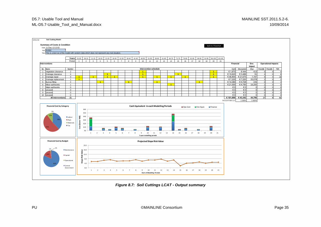
8.4.1 Output Summary (Figure 8.7)
This worksheet is the main output of the model which concludes all the information for the user. It gives an overview of the interventions employed, the overall costs and impacts, and summary charts of the projected cash equivalent expenditure and asset condition.
8.4.2 Output Financial (Figure 8.8)
This worksheet focuses on the financial costs associated with the intervention plan of the asset over the next 100 years.
It gives more detail of the cash flow in terms of cash costs as well as cash equivalents of the environmental and operational impacts. These results can be shown with or without discounting over the 100-year period.
8.4.3 Output Environmental (Figure 8.9)
This worksheet summarises the environmental aspects of the intervention plan of the asset over the projected time of 100 years.
It shows the summary of the environmental impacts as CO2 emissions resulting from each of the interventions used and the total impact in each modelling period.
8.4.4 Output Operations (Figure 8.10)
This worksheet tabulates the operational impacts (i.e. possession costs) due to the required intervention plan.
It shows the summary of the operational impacts resulting from each of the interventions used and the total impact in each modelling period.
8.4.5 Output Condition (Figure 8.11)
The final output worksheet concentrates on the service condition of the asset.
It shows the projection of the various conditions and performance measures of the asset over time. More specifically, it provides information about the condition of the asset under all the six MAINLINE Algorithm sub-assessments (sub-scores) as well as the final SRV score condition.
D5.7: Usable Tool and Manual MAINLINE SST.2011.5.2-6.
ML-D5.7-Usable_Tool_and_Manual.docx 10/09/2014
PU ©MAINLINE Consortium Page 35
Figure 8.7: Soil Cuttings LCAT - Output summary
MAINLINE Soil Cutting Model
Summary of Costs & Condition
Date 11-Dec-13 13:02
Ref: RV002
Title:
Years: 01-05 06-10 11-15 16-20 21-25 26-30 31-35 36-40 41-45 46-50 51-55 56-60 61-65 66-70 71-75 76-80 81-85 86-90 91-95 96-100 101-05
Period: 1 2 3 4 5 6 7 8 9 10 11 12 13 14 15 16 17 18 19 20 21
Env.
Impact
No Name Number Cash Discounted CO2e Poss(N) Poss(D) TSR
1 Vegetation clearance 2 0 0 0 0 0 0 0 0 0 1 0 0 0 0 0 0 0 0 0 1 0 € 1,870 € 444 413 0 0 4
2 Drainage clearance 4 0 0 0 0 1 0 0 0 0 1 0 0 0 0 1 0 0 0 0 1 0 € 10,620 € 3,486 91 4 0 8
3 Drainage repair 9 1 0 1 0 1 1 0 0 0 1 0 1 0 1 0 1 0 0 0 1 0 € 46,800 € 21,675 7,787 9 0 18
4 Drainage replacement 1 1 0 0 0 0 0 0 0 0 0 0 0 0 0 0 0 0 0 0 0 0 € 7,220 € 7,220 20,078 2 0 2
5 Burrow filling 4 0 0 0 1 0 0 0 1 0 0 0 1 0 0 0 0 0 1 0 0 0 € 14,380 € 5,728 226 0 0 4
6 Minor earthworks 1 0 0 0 0 0 0 0 0 0 0 0 0 0 1 0 0 0 0 0 0 0 € 21,000 € 4,790 16,200 2 0 5
7 Major earthworks 0 0 0 0 0 0 0 0 0 0 0 0 0 0 0 0 0 0 0 0 0 0 € 0 € 0 0 0 0 0
8 [unused] 0 0 0 0 0 0 0 0 0 0 0 0 0 0 0 0 0 0 0 0 0 0 € 0 € 0 0 0 0 0
9 [unused] 0 0 0 0 0 0 0 0 0 0 0 0 0 0 0 0 0 0 0 0 0 0 € 0 € 0 0 0 0 0
10 [unused] 0 0 0 0 0 0 0 0 0 0 0 0 0 0 0 0 0 0 0 0 0 0 € 0 € 0 0 0 0 0
21 € 101,890 € 43,342 44,795 17 0 41
Discount rates p.a. 2.300% 2.000%
Costs by Category
Labour 38,500
Plant 52,700
Materials 10,690
Tax 0
Costs by Budget
Maintenance 83,340
Capital 16,450
Operational 1,050
Central Government 1,050
Operational Impacts
All interventions
Intervention schedule
This is a test run of the model with random data which does not represent any real situation.
Interventions Financial
0.0
4.0
8.0
12.0
16.0
20.0
1 2 3 4 5 6 7 8 9 10 11 12 13 14 15 16 17 18 19 20 21
Slo
pe
Ris
k V
alu
e
Start of Modelling Periods
Projected Slope Risk Value
€0
€10
€20
€30
€40
€50
€60
1 2 3 4 5 6 7 8 9 10 11 12 13 14 15 16 17 18 19 20 21
Co
st [
Euro
s '0
00]
5-year modelling periods
Cash Equivalent in each Modelling Periods Ops Cost Env Equiv Finance
38%
52%
10%
0%
Financial Cost by Category
Labour
Plant
Materials
Tax
82%
16%
1%1%
Financial Cost by Budget
Maintenance
Capital
Operational
CentralGovernment
back to: Flowchart

D5.7: Usable Tool and Manual MAINLINE SST.2011.5.2-6.
ML-D5.7-Usable_Tool_and_Manual.docx 10/09/2014
PU ©MAINLINE Consortium Page 36
Figure 8.8: Soil Cuttings LCAT - Financial output
MAINLINE Soil Cutting Model
Summary of Projected Costs
Date: 11/12/2013 13:02
Ref: RV002
Title: This is a test run of the model with random data which does not represent any real situation.
Years: 01-05 06-10 11-15 16-20 21-25 26-30 31-35 36-40 41-45 46-50 51-55 56-60 61-65 66-70 71-75 76-80 81-85 86-90 91-95 96-100 101-05
Period: 1 2 3 4 5 6 7 8 9 10 11 12 13 14 15 16 17 18 19 20 21
No Name
1 Vegetation clearance 0 0 0 0 0 0 0 0 0 1 0 0 0 0 0 0 0 0 0 1 0
2 Drainage clearance 0 0 0 0 1 0 0 0 0 1 0 0 0 0 1 0 0 0 0 1 0
3 Drainage repair 1 0 1 0 1 1 0 0 0 1 0 1 0 1 0 1 0 0 0 1 0
4 Drainage replacement 1 0 0 0 0 0 0 0 0 0 0 0 0 0 0 0 0 0 0 0 0
5 Burrow filling 0 0 0 1 0 0 0 1 0 0 0 1 0 0 0 0 0 1 0 0 0
6 Minor earthworks 0 0 0 0 0 0 0 0 0 0 0 0 0 1 0 0 0 0 0 0 0
7 Major earthworks 0 0 0 0 0 0 0 0 0 0 0 0 0 0 0 0 0 0 0 0 0
8 [unused] 0 0 0 0 0 0 0 0 0 0 0 0 0 0 0 0 0 0 0 0 0
9 [unused] 0 0 0 0 0 0 0 0 0 0 0 0 0 0 0 0 0 0 0 0 0
10 [unused] 0 0 0 0 0 0 0 0 0 0 0 0 0 0 0 0 0 0 0 0 0
Cash Equivalent Costs (€'000) Total
Finance €k 12 €k 0 €k 5 €k 4 €k 8 €k 5 €k 0 €k 4 €k 0 €k 9 €k 0 €k 9 €k 0 €k 26 €k 3 €k 5 €k 0 €k 4 €k 0 €k 9 €k 0 €k 102
Env Equiv €k 21 €k 0 €k 1 €k 0 €k 1 €k 1 €k 0 €k 0 €k 0 €k 1 €k 0 €k 1 €k 0 €k 17 €k 0 €k 1 €k 0 €k 0 €k 0 €k 1 €k 0 €k 45
Ops Cost €k 4 €k 0 €k 1 €k 0 €k 3 €k 1 €k 0 €k 0 €k 0 €k 3 €k 0 €k 2 €k 0 €k 4 €k 1 €k 1 €k 0 €k 0 €k 0 €k 3 €k 0 €k 25
Total € 37 € 0 € 7 € 4 € 12 € 7 € 0 € 4 € 0 € 13 € 0 € 11 € 0 € 48 € 4 € 7 € 0 € 4 € 0 € 13 €k 0 €k 172
Discounted Costs (€'000)
2.30% p.a. Finance €k 12 €k 0 €k 4 €k 3 €k 5 €k 3 €k 0 €k 2 €k 0 €k 3 €k 0 €k 3 €k 0 €k 6 €k 1 €k 1 €k 0 €k 1 €k 0 €k 1 €k 0 €k 43
2.00% p.a. Env Equiv €k 21 €k 0 €k 1 €k 0 €k 1 €k 1 €k 0 €k 0 €k 0 €k 0 €k 0 €k 0 €k 0 €k 5 €k 0 €k 0 €k 0 €k 0 €k 0 €k 0 €k 0 €k 29
2.30% p.a. Ops Cost €k 4 €k 0 €k 1 €k 0 €k 2 €k 1 €k 0 €k 0 €k 0 €k 1 €k 0 €k 0 €k 0 €k 1 €k 0 €k 0 €k 0 €k 0 €k 0 €k 0 €k 0 €k 11
Total €k 37 €k 0 €k 6 €k 3 €k 7 €k 4 €k 0 €k 2 €k 0 €k 5 €k 0 €k 3 €k 0 €k 12 €k 1 €k 1 €k 0 €k 1 €k 0 €k 2 €k 0 €k 83
Chart options:
FALSE Finance €k 12 €k 0 €k 5 €k 4 €k 8 €k 5 €k 0 €k 4 €k 0 €k 9 €k 0 €k 9 €k 0 €k 26 €k 3 €k 5 €k 0 €k 4 €k 0 €k 9 €k 0
TRUE Env Equiv €k 21 €k 0 €k 1 €k 0 €k 1 €k 1 €k 0 €k 0 €k 0 €k 1 €k 0 €k 1 €k 0 €k 17 €k 0 €k 1 €k 0 €k 0 €k 0 €k 1 €k 0
TRUE Ops Cost €k 4 €k 0 €k 1 €k 0 €k 3 €k 1 €k 0 €k 0 €k 0 €k 3 €k 0 €k 2 €k 0 €k 4 €k 1 €k 1 €k 0 €k 0 €k 0 €k 3 €k 0
Interventions
€k 0
€k 10
€k 20
€k 30
€k 40
€k 50
€k 60
1 2 3 4 5 6 7 8 9 10 11 12 13 14 15 16 17 18 19 20 21
Co
st [
Euro
s '0
00]
5-year modelling periods
Cash Equivalent in each Modelling Periods Ops Cost Env Equiv Finance
Show discounted
Include Env. Impacts
Include Ops. Impacts
back to: Flowchart

D5.7: Usable Tool and Manual MAINLINE SST.2011.5.2-6.
ML-D5.7-Usable_Tool_and_Manual.docx 10/09/2014
PU ©MAINLINE Consortium Page 37
Figure 8.9: Soil Cuttings LCAT - Environmental output
MAINLINE Soil Cutting Model
Summary of Projected Environmental Impacts
Date: 11/12/2013 13:02
Ref: RV002
Title: This is a test run of the model with random data which does not represent any real situation.
Years: 01-05 06-10 11-15 16-20 21-25 26-30 31-35 36-40 41-45 46-50 51-55 56-60 61-65 66-70 71-75 76-80 81-85 86-90 91-95 96-100 101-05
Environmental Impacts Period: 1 2 3 4 5 6 7 8 9 10 11 12 13 14 15 16 17 18 19 20 21
No Name Total
1 Vegetation clearance 0 0 0 0 0 0 0 0 0 207 0 0 0 0 0 0 0 0 0 207 0 413
2 Drainage clearance 0 0 0 0 23 0 0 0 0 23 0 0 0 0 23 0 0 0 0 23 0 91
3 Drainage repair 865 0 865 0 865 865 0 0 0 865 0 865 0 865 0 865 0 0 0 865 0 7,787
4 Drainage replacement 20,078 0 0 0 0 0 0 0 0 0 0 0 0 0 0 0 0 0 0 0 0 20,078
5 Burrow filling 0 0 0 56 0 0 0 56 0 0 0 56 0 0 0 0 0 56 0 0 0 226
6 Minor earthworks 0 0 0 0 0 0 0 0 0 0 0 0 0 16,200 0 0 0 0 0 0 0 16,200
7 Major earthworks 0 0 0 0 0 0 0 0 0 0 0 0 0 0 0 0 0 0 0 0 0 0
8 [unused] 0 0 0 0 0 0 0 0 0 0 0 0 0 0 0 0 0 0 0 0 0 0
9 [unused] 0 0 0 0 0 0 0 0 0 0 0 0 0 0 0 0 0 0 0 0 0 0
10 [unused] 0 0 0 0 0 0 0 0 0 0 0 0 0 0 0 0 0 0 0 0 0 0
20,943 0 865 56 888 865 0 56 0 1,095 0 922 0 17,065 23 865 0 56 0 1,095 0 44,795
Emissions of Carbon Dioxide (equivalent) CO2e kg
0
5,000
10,000
15,000
20,000
25,000
1 2 3 4 5 6 7 8 9 10 11 12 13 14 15 16 17 18 19 20 21
kg o
f C
O2
Eq
uiv
ale
nt
Modelling period
Environmental Impacts - shown for each Intervention Type[unused]
[unused]
[unused]
Major earthworks
Minor earthworks
Burrow filling
Drainage replacement
Drainage repair
Drainage clearance
Vegetation clearance
back to: Flowchart

D5.7: Usable Tool and Manual MAINLINE SST.2011.5.2-6.
ML-D5.7-Usable_Tool_and_Manual.docx 10/09/2014
PU ©MAINLINE Consortium Page 38
Figure 8.10: Soil Cuttings LCAT - Operational output
MAINLINE Soil Cutting Model
Summary of Projected Costs & Impacts
Date: 11/12/2013 13:44
Ref: RV002
Title: This is a test run of the model with random data which does not represent any real situation.
Years: 01-05 06-10 11-15 16-20 21-25 26-30 31-35 36-40 41-45 46-50 51-55 56-60 61-65 66-70 71-75 76-80 81-85 86-90 91-95 96-100 101-05
Period: 1 2 3 4 5 6 7 8 9 10 11 12 13 14 15 16 17 18 19 20 21
No Name
1 Vegetation clearance 0 0 0 0 0 0 0 0 0 1 0 0 0 0 0 0 0 0 0 1 0
2 Drainage clearance 0 0 0 0 1 0 0 0 0 1 0 0 0 0 1 0 0 0 0 1 0
3 Drainage repair 1 0 1 0 1 1 0 0 0 1 0 1 0 1 0 1 0 0 0 1 0
4 Drainage replacement 1 0 0 0 0 0 0 0 0 0 0 0 0 0 0 0 0 0 0 0 0
5 Burrow filling 0 0 0 1 0 0 0 1 0 0 0 1 0 0 0 0 0 1 0 0 0
6 Minor earthworks 0 0 0 0 0 0 0 0 0 0 0 0 0 1 0 0 0 0 0 0 0
7 Major earthworks 0 0 0 0 0 0 0 0 0 0 0 0 0 0 0 0 0 0 0 0 0
8 [unused] 0 0 0 0 0 0 0 0 0 0 0 0 0 0 0 0 0 0 0 0 0
9 [unused] 0 0 0 0 0 0 0 0 0 0 0 0 0 0 0 0 0 0 0 0 0
10 [unused] 0 0 0 0 0 0 0 0 0 0 0 0 0 0 0 0 0 0 0 0 0
Operational Impacts Total
Over-night possession [Nr] Poss(N) 3 0 1 0 2 1 0 0 0 2 0 1 0 3 1 1 0 0 0 2 0 17
Day possessions [Nr] Poss(D) 0 0 0 0 0 0 0 0 0 0 0 0 0 0 0 0 0 0 0 0 0 0
Speed restriction [days] TSR 4 0 2 1 4 2 0 1 0 6 0 3 0 7 2 2 0 1 0 6 0 41
Interventions
0
1
2
3
4
5
6
7
8
1 2 3 4 5 6 7 8 9 10 11 12 13 14 15 16 17 18 19 20 21
Op
era
tio
na
l Im
pa
ct
5-year modelling periods
Operational Impacts in each Modelling Periods
Poss(N)
Poss(D)
TSR
back to: Flowchart

D5.7: Usable Tool and Manual MAINLINE SST.2011.5.2-6.
ML-D5.7-Usable_Tool_and_Manual.docx 10/09/2014
PU ©MAINLINE Consortium Page 39
Figure 8.11: Soil Cuttings LCAT - Condition output
MAINLINE Soil Cutting Model
Summary of Projected Condition
Date: 11/12/2013 13:44
Ref: RV002
Title: This is a test run of the model with random data which does not represent any real situation.
Years: 01-05 06-10 11-15 16-20 21-25 26-30 31-35 36-40 41-45 46-50 51-55 56-60 61-65 66-70 71-75 76-80 81-85 86-90 91-95 96-100 101-05
Period: 1 2 3 4 5 6 7 8 9 10 11 12 13 14 15 16 17 18 19 20 21
No Name
1 Vegetation clearance 0 0 0 0 0 0 0 0 0 1 0 0 0 0 0 0 0 0 0 1 0
2 Drainage clearance 0 0 0 0 1 0 0 0 0 1 0 0 0 0 1 0 0 0 0 1 0
3 Drainage repair 1 0 1 0 1 1 0 0 0 1 0 1 0 1 0 1 0 0 0 1 0
4 Drainage replacement 1 0 0 0 0 0 0 0 0 0 0 0 0 0 0 0 0 0 0 0 0
5 Burrow filling 0 0 0 1 0 0 0 1 0 0 0 1 0 0 0 0 0 1 0 0 0
6 Minor earthworks 0 0 0 0 0 0 0 0 0 0 0 0 0 1 0 0 0 0 0 0 0
7 Major earthworks 0 0 0 0 0 0 0 0 0 0 0 0 0 0 0 0 0 0 0 0 0
8 [unused] 0 0 0 0 0 0 0 0 0 0 0 0 0 0 0 0 0 0 0 0 0
9 [unused] 0 0 0 0 0 0 0 0 0 0 0 0 0 0 0 0 0 0 0 0 0
10 [unused] 0 0 0 0 0 0 0 0 0 0 0 0 0 0 0 0 0 0 0 0 0
Condition Scores
MA Movement Assessment 3.0 3.1 3.2 3.2 3.3 3.4 3.5 3.5 3.6 3.7 3.8 3.8 3.9 4.0 1.5 2.6 2.7 2.8 2.9 3.0 3.0
VA Vegetation Assessment 0.0 0.3 0.9 1.2 1.2 1.2 1.3 1.3 1.3 1.4 0.0 0.3 0.9 1.2 0.0 0.3 0.9 1.2 1.2 1.2 0.0
SW Surface Water Assessment 1.0 0.6 0.8 0.6 0.9 0.1 0.0 0.3 0.5 0.8 0.1 0.4 0.1 0.4 0.0 0.0 0.0 0.3 0.5 0.8 0.1
DA Drainage Assessment 1.0 0.0 0.2 0.0 0.2 0.5 0.0 0.2 0.3 0.5 0.2 0.4 0.0 0.2 0.0 0.5 0.0 0.2 0.3 0.5 0.2
BA Burrowing Assessment 0.0 0.5 1.0 1.5 0.0 0.5 1.0 1.5 0.0 0.5 1.0 1.5 0.0 0.5 0.0 0.5 1.0 1.5 0.0 0.5 1.0
CA Construction Activity Assessment 1.0 1.0 1.1 1.1 1.1 1.1 1.2 1.2 1.2 1.2 1.3 1.3 1.3 1.3 0.0 0.0 0.1 0.1 0.2 0.2 0.3
SRV Slope Risk Value 5.5 5.7 6.6 7.0 5.8 6.1 6.2 7.1 5.9 6.9 6.8 7.7 5.9 6.9 1.7 4.1 4.2 5.2 4.0 4.9 4.9
Interventions
-1.0
0.0
1.0
2.0
3.0
4.0
5.0
6.0
7.0
8.0
9.0
1 2 3 4 5 6 7 8 9 10 11 12 13 14 15 16 17 18 19 20 21
Co
nd
itio
n S
core
s
5-year Modelling Periods
Projected Condition Scores
MA VA
SW DA
BA CA
SRV
back to: Flowchart

D5.7: Usable Tool and Manual MAINLINE SST.2011.5.2-6.
ML-D5.7-Usable_Tool_and_Manual.docx 10/09/2014
PU ©MAINLINE Consortium Page 40
8.4.6 Summary of outputs
The upper part of Figure 8.7 shows the intervention schedule followed by the cash equivalents in each 5 year period.
The lower part of Figure 8.7 shows the projected slope risk value of the soil cutting produced by the MAINLINE Algorithm (remind that lower values, result to better asset condition). In this example, it is seen that a minor intervention of the asset coupled with a drainage repair at period 14, result in a significant improvement in the condition of the cutting.
In Error! Reference source not found. Figure 8.8, the financial costs of the intervention lan of Figure 8.7 can be demonstrated in a discount rate (the rate is specified by the user), which is the preferred measure for comparison of different maintenance strategies.
Figures 8.9, 8.10 and 8.11 provide more detailed information about the operational and environmental impacts of the proposed intervention plan and how these are translated into cash as well as the performance of the cutting through time.
Last but not least, for a validation of the model with real case studies, the user may reference the Cuttings section of ML D5.6 (MAILINE, 2014b).

D5.7: Usable Tool and Manual MAINLINE SST.2011.5.2-6.
ML-D5.7-Usable_Tool_and_Manual.docx 10/09/2014
PU ©MAINLINE Consortium Page 41
9. Metallic Bridges LCAT
9.1 Assumptions and modelling techniques
The Bridges LCAT is a decision support tool that compares different maintenance and renewal strategies for metallic bridges based on a life cycle evaluation and attempts to quantify the costs and risks associated with such strategies over a period of one hundred years.
9.1.1 Bridges LCAT application
This tool processes a single element of a metallic bridge at a time, correlating condition and capacity. Multiple runs of the LCAT tool may be required on a number of the bridge elements to establish the optimum strategy for the entire bridge.
A typical short span metallic bridge and its main elements can be seen in the Figure 9.1.
Figure 9.1: Short span metallic bridge
9.1.2 Deterioration modelling techniques
The modelling of degradation of metallic bridges is deterministic and based on the assumption that an element’s coating deteriorates first and corrosion follows if the element is left unpainted. The LCAT assumes uniform and averaged degradation of coating and uniform intervention or at least correlation between capacity governing cross sections and degradation (MAILINE, 2013).

D5.7: Usable Tool and Manual MAINLINE SST.2011.5.2-6.
ML-D5.7-Usable_Tool_and_Manual.docx 10/09/2014
PU ©MAINLINE Consortium Page 42
Figure 9.2: Bridge deterioration mechanism
In ML D2.3 (MAILINE, 2013) theoretical degradation profiles that process coating loss and corrosion depth of an element to calculate the projected thickness loss have been developed and quantified. This report concentrates on the main features of this detailed analysis.
That being said, the Bridges LCAT features two ancillary worksheets (‘Reference’ and ‘Assumptions’), to introduce the concepts and assumptions being made for corrosion and coating deterioration modelling techniques.
These ancillary worksheets are briefly discussed in the following pages, before moving on the function of the model.
Corrosivity categories
In ML D2.3 (MAILINE, 2013) coating deterioration and steel corrosion (following the loss of protection provided by the coating) are time-dependent processes, with their rate being determined by the exposure conditions experienced by the bridge. The possible types of outdoor exposure environments that may be experienced by a structure can be broadly classified under as: (a) immersed, (b) splash zone and (c) atmospheric exposure. Each of these environments is associated with different ranges of corrosivity potential. Atmospheric exposure can itself be subdivided in a number of categories based on their corrosivity harshness, represented as rural, urban and industrial/marine exposures.
Further, ML D2.3 (MAILINE, 2013) concluded that the main parameters influencing the corrosivity of an atmosphere include climatic factors (i.e. relative humidity and temperature) and atmospheric pollutants (i.e. sulphur dioxide (SO2) and chlorides (Cl-)). The physical monitoring of these parameters would enable the atmospheric corrosivity classification of a particular area.
The standard EN ISO 9223 provides a framework for the classification of atmospheric corrosivity based on the levels of the main influencing climatic and pollutant parameters. More specifically, in EN ISO 9223, the spectrum of atmospheric corrosivity is divided into five categories varying from very low corrosivity (category C1), corresponding to rural environments, up to very high corrosivity (C5) and extreme corrosivity (CX).

D5.7: Usable Tool and Manual MAINLINE SST.2011.5.2-6.
ML-D5.7-Usable_Tool_and_Manual.docx 10/09/2014
PU ©MAINLINE Consortium Page 43
Corrosivity category
Description Corrosion rates 1
(mm/year)
C1 Very low corrosivity: Dry or cold zone, atmospheric environment with very low pollution and time of wetness, e.g. certain deserts, Central Arctic/Antarctica.
≤ 0.0013
C2 Low corrosivity: Temperate zone, atmospheric environment with low pollution (SO2 < 5 μg/m
3), e.g. rural areas, small towns. Dry or
cold zone, atmospheric environment with short time of wetness, e.g. deserts, subarctic areas.
0.0013 < A ≤ 0.025
C3 Medium corrosivity: Temperate zone, atmospheric environment with medium pollution (SO2: 5 μg/m
2 to 30 μg/m
3) or some effect
of chlorides, e.g. urban areas, coastal areas with low deposition of chlorides. Subtropical and tropical zone, atmosphere with low pollution.
0.025 < A ≤ 0.050
C4 High corrosivity: Temperate zone, atmospheric environment with high pollution (SO2: 30 μg/m
3 to 90 μg/m
3) or substantial effect of
chlorides, e.g. polluted urban areas, industrial areas, coastal areas without spray of salt water or, exposure to effect of de-icing salts. Subtropical and tropical zone, atmosphere with medium pollution.
0.050 < A ≤ 0.080
C5 Very high corrosivity: Temperate and subtropical zone, atmospheric environment with very high pollution (SO2: 90 μg/m
3
to 250 μg/m3) and/or significant effect of chlorides, e.g. industrial
areas, coastal areas, sheltered positions on coastline.
0.080 < A ≤ 0.200
CX Extreme corrosivity: Subtropical and tropical zone (very high time of wetness), atmospheric environment with high SO2 pollution (higher than 250 μg/m
3) including accompanying and
production factors and/or strong effect of chlorides, e.g. extreme industrial areas, coastal and offshore areas, occasional contact with salt spray.
0.200 < A ≤ 0.700
Notes: 1 Corrosion rates correspond to the first year of exposure
Therefore, this framework has been employed by the Bridges LCAT to classify corrosivity parameters. Table 9.1 below is taken from the ‘Reference’ sheet of the model and illustrates and concept discussed above.
The user is advised to read this framework and appreciate the different corrosivity categories. For the purposes of the prototype LCAT, C1, C2, C3 and C5 corrosivity categories have been used. This can be changed with further customization of the model.
Furthermore, in considering the deterioration of complex and spatially extended structural systems such as bridges, individual elements (e.g. deck, main girders, cross beams, etc.) are likely to experience dissimilar deterioration rates due to differences in the microclimate which develops in their immediate surroundings (MAILINE, 2013). Hence, a study has been conducted to take microclimate into account and its results, which are shown in the Table 1 of the ‘Assumptions’ sheet, can be seen in Table 9.2:
Table 9.1: Description of atmospheric corrosivity categories and corresponding corrosion rates (MAILINE, 2013)

D5.7: Usable Tool and Manual MAINLINE SST.2011.5.2-6.
ML-D5.7-Usable_Tool_and_Manual.docx 10/09/2014
PU ©MAINLINE Consortium Page 44
Coating system name
Description
Expected life, LT (years)
M27.4 Protective system using bitumen. 1st layer: surface tolerant epoxy
primer (min dft 100μm. Intermediate coat: gelled bituminous solution – aluminium tinted (min dft 200μm). Topcoat: gelled bituminous solution – black finish with min dft 200μm.
5-7
M21 Coating using epoxy glass flake. 1st layer: epoxy blast primer with
min dft 25μm. Intermediate layer: epoxy glass flake intermediate coat with min dft 40μm and for layer C select among the following (min dft 50μm): anti-graffiti paint or polyurethane coloured finish or acrylic urethane topcoat or polysiloxane topcoat.
18-22
Table 9.2: Exposure conditions assumed for bridge Elements
Element exposure Box
Bridge environment Exposed Protected Section
Rural (C2) C2 C1 C1
Urban (C3) C3 C2 C2
Industrial (C5) C5 C3 C2
Coating systems
Data for the expected service life of different coating systems currently used in the UK railway infrastructure (Network Rail) has been applied in the model. Nonetheless several coating types – of varying composition and performance – exist for the protection of structural steelwork across Europe, so in the light of field data, the model can be customized and the user may enter different coating types and service lives.
The following framework is taken from the ‘Reference’ sheet of the LCAT and shows the coating information that the model uses by default. However, as it was mentioned, the user can apply different coating systems and see the performance of the asset under multiple conditions. As a side note, VBA programming has been employed to accommodate this dynamic change of the coating data, adding further flexibility and customization to the end user. The VBA code (macro) can be reviewed in the Appendix 14.2.
Coating deterioration
In this section, a framework for deterioration modelling of the coating-steel substrate system is presented, which is in line with the exposure classification recommendations of EN ISO 9223 (ISO, 2012). For more detailed information, the user is advised to read ML D2.3 (MAILINE, 2013).
Corrosion will begin to affect exposed steel surfaces immediately if no coating is applied, or after some time if coating has been applied, in places where the coating becomes ineffective. The coating itself will gradually deteriorate with time (i.e. the protected steel surface area reduces with time) and eventually it will become completely ineffective. The time-dependent coating performance is by default modelled using information available in Network Rail
Table 9.3: Description and expected service life of protective coatings (ML D2.3)

D5.7: Usable Tool and Manual MAINLINE SST.2011.5.2-6.
ML-D5.7-Usable_Tool_and_Manual.docx 10/09/2014
PU ©MAINLINE Consortium Page 45
100
50
Time (years)
(%) protected
area
Linear
deterioration
Non-linear
deterioration
TU TL
Coating
reapplication
standard NR/L3/CIV/040 where a range of expected life (TL) values are provided for a number of coatings used in the UK (see ML D2.3 (MAILINE, 2013) for more details). The user may define service lives for other coating types that suits her needs.
A simple polynomial model (Equation 9.1) is developed, based on the assumption that 50% of the coated steel area will become unprotected at time TL, shown schematically in Fig.9.3.
Apr t
Apr0=1 −
0.6t 2
TL2 −
0.1t
TL (9.1)
where, Apr(t) and Apr0 are the residual and initial protected area, respectively and t is the time in years. This model is used to predict the time TU at which the entire coating is lost (and hence the entire underlying steel surface is actively corroding). Note that Apr(t) ≤ Apr0 for all t and Apr(t) = 0 for t > TU.
Atmospheric corrosion deterioration modelling
As presented in ML D2.2 (MAILINE, 2012b), the progress of atmospheric corrosion can be
modelled in terms of thickness loss using a power expression (MAILINE, 2013).
BC t At (9.2)
where, C(t) is the uniform (measured as average over relatively small specimen surface areas) thickness loss (mm) after an exposure period of t years and coefficients A (mm/year) and B are empirical constants, obtained using regression analysis on physical test results grouped according to different atmospheric exposure conditions.
Figure 9.3: Deterioration model for coating system

D5.7: Usable Tool and Manual MAINLINE SST.2011.5.2-6.
ML-D5.7-Usable_Tool_and_Manual.docx 10/09/2014
PU ©MAINLINE Consortium Page 46
Table 9.4, taken from the ‘Reference’ sheet, summarises the corrosion parameters under different corrosivity categories (i.e. C1-C5). These factors are used to calculate corrosion depth of an element and thickness loss, when coating protection is not applied.
Table 9.4: Parameters assumed for exposure conditions of bridge Elements.
(Coating name and service lives shown are default values that may be modified by the user)
Parameters
Element Exposure
Coating service life TL (years) Corrosion
NC M27.4 M21 A (mm) B t1 (years)
C1 0 7 22 0.0013 0.5750 20
C2 0 7 22 0.0250 0.5750 20
C3 0 6 20 0.0500 0.5750 20
C5 0 5 18 0.2000 0.5750 20
9.1.3 Further assumptions
Similar to the Soil Cuttings LCAT, the Bridges LCAT does not have a length dimension. It can accommodate any length; the user may specify the appropriate length based on relevant cost information.
In terms of the modelled interventions, the tool is not fully flexible. It has been pre-programmed to incorporate three intervention strategies:
(a) Strengthening (planting) of element
(b) Repainting (coating) of element
(c) Replacement (on a like-for-like basis) of an element
The user is allowed to switch on/off these intervention strategies, depending on what is to be examined in a life cycle evaluation, but further interventions cannot be added in this prototype version of the model. To sum up, the table below summarises the points discussed above.

D5.7: Usable Tool and Manual MAINLINE SST.2011.5.2-6.
ML-D5.7-Usable_Tool_and_Manual.docx 10/09/2014
PU ©MAINLINE Consortium Page 47
Table 9.5: Bridges LCAT assumptions
LCAT model
Modelled element
Modelled parameters
Modelling approach
Interventions Time step
Metallic Bridges
One bridge element
Coating coverage
Deterministic
Strengthening
Annual
Corrosion depth
Coating
Replacement
The section walks the user through the algorithmic process of the ‘inputs-calculations-outputs’ that the tool employs and demonstrate how the tool actually works by presenting typical screenshots.
For a tutorial of the model using real case studies, the user is encouraged to read Appendix 14.4, which contains the slides form the demonstration of the LCAT in the MAINLINE training sessions and the ML D5.6 document (MAILINE, 2014b).
9.2 Inputs of data
Like the Soil Cutting LCAT, the Metallic Bridges LCAT requires four different input categories:
- Initial asset condition - Intervention triggers - Uplift effects - Costs of interventions and environmental impacts
Data for which are entered into the blue colour cells.
9.2.1 Input of initial asset condition
The first data requirement is the condition of the underlying bridge at the start of the model run. There are three sections of input data.
(a) Bridge environment The overall operating environment of the bridge needs to be assessed and entered in the model. There are three types of environment, depending on the atmospheric pollution: rural, urban, industrial. There is a drop down list and the user needs to select which of these is closest to reality. The specification of the surrounding environment references the corrosivity categories which are later used to calculate corrosion depth estimates.
(b) Element Details

D5.7: Usable Tool and Manual MAINLINE SST.2011.5.2-6.
ML-D5.7-Usable_Tool_and_Manual.docx 10/09/2014
PU ©MAINLINE Consortium Page 48
The element details and dimensions need to be specified. The type of the element (I-beam, box section or channel) as well as its overall dimensions in millimetres (i.e. depth and breadth) should be defined. An element name and ID should be given according to user’s information. Finally, the element is broken down to its component parts (i.e. if it is I-beam, these are flanges and web) and the nominal and initial thickness of these parts need to be determined (in millimetres). This information allows the model to start the modelling from a condition different to the element’s nominal (perfect) condition. Nominal is the original thickness of the element, whereas, initial, is the thickness at the start of the model run (which might be different due to tolerances from fabrication or if deterioration has been applied).
(c) Coating Details The last section of the initial asset condition is regarding coating data. It is divided into two sub-sections
- Coating details: This may or may not be a user input. Depending on the availability of relevant data the user may choose to click the ‘YES’ button and insert coating names and expected service lives. It should be noted that up to two coating types can be defined. Alternatively, the user may click the ‘NO’ button and default coating data from the UK infrastructure will be used to calculate coating deterioration.
- Initial coating: Based on the above mentioned coating information, the starting coating condition of the element should be determined. Either the age of the coating (in years) or the percentage of the initial coating coverage should be inserted. If both of them are entered, the percentage would take precedence.

D5.7: Usable Tool and Manual MAINLINE SST.2011.5.2-6.
ML-D5.7-Usable_Tool_and_Manual.docx 10/09/2014
PU ©MAINLINE Consortium Page 49
Figure 9.4: Bridges LCAT - Initial condition
9.2.2 Input of intervention triggers
Intervention strategies are listed on this worksheet and the user may select/adjust the scores at which interventions may be triggered. As mentioned above, there are three pre-set interventions built into the model: (a) strengthening (b) coating (c) replacement.
Each intervention may be initiated by a score value (typically percentage) and these ‘trigger scores’ are input on this worksheet. Alternatively, the user may specify times when the interventions are to be used (i.e. for example intervention No.1 should be applied every ten years).

D5.7: Usable Tool and Manual MAINLINE SST.2011.5.2-6.
ML-D5.7-Usable_Tool_and_Manual.docx 10/09/2014
PU ©MAINLINE Consortium Page 50
To avoid interventions being initialised at the same time, logical rules have been incorporated to prioritize interventions. These are as follows:
(a) if replacement happens to occur in the same year with any of the other two interventions - replacement will take precedence
(b) If strengthening happens to occur in the same year with recoating - Strengthening will take precedence
A set of seven triggers are associated with condition and capacity intervention strategies relating to:
- Bending resistance - Shear resistance - Axial resistance - Local buckling resistance
These triggers can be switched on or off for each of the three interventions. In the example below the three pre-set interventions are illustrated as well as how they can be triggered variously by percentage change in attributes or by and user-specified timings.

D5.7: Usable Tool and Manual MAINLINE SST.2011.5.2-6.
ML-D5.7-Usable_Tool_and_Manual.docx 10/09/2014
PU ©MAINLINE Consortium Page 51
Figure 9.5: Metallic Bridges LCAT - Intervention triggers

D5.7: Usable Tool and Manual MAINLINE SST.2011.5.2-6.
ML-D5.7-Usable_Tool_and_Manual.docx 10/09/2014
PU ©MAINLINE Consortium Page 52
9.2.3 Changes caused by interventions (uplift effects)
Interventions are applied to the asset in order to change its condition, improving/restoring its coating and corrosion (thickness loss) performance. The model allows the user to partially input what each intervention is expected to achieve (uplift effects after intervention).
Figure 9.6 shows how the user defines the interventions are applied.
Figure 9.6: Bridges LCAT – Uplift effects
It should be noted that an intervention may affect either coating or thickness adjustment (change of element thickness) or both of them. As shown above, coating and corrosion uplift effects have been split into two matrices and the user has partially got the option to switch on/off what each intervention is expected to do (i.e. when recoating is initialized which coating system may be used).
What is more, some logical assumptions have been pre-programmed into the model. These are mainly the following:
- New coatings are assumed to completely replace any existing ones - Replacement is assumed to completely replace the element (on a like-for-like basis) - Replacement is assumed to reset the thickness of the element to its nominal value
9.2.4 Input of intervention costs
The costs and impacts of each intervention are summarised on the Intervention Costs worksheet below (‘IntvCosts’ – Figure 9.7), but details of the costs and environmental impacts are input on a separate, more detailed worksheet for each of the three interventions called ‘IntvCost(1)’, ‘IntvCost(2)’ and ‘IntvCost(3)’.

D5.7: Usable Tool and Manual MAINLINE SST.2011.5.2-6.
ML-D5.7-Usable_Tool_and_Manual.docx 10/09/2014
PU ©MAINLINE Consortium Page 53
On the cost summary sheet the user may specify cost categories and budgets which may be chosen to suit the user’s own financial arrangements.
Also on the cost summary worksheet the user may identify some operational (e.g. possession costs) and environmental impacts which will arise when the intervention is executed. These may be selected by the user.
An operational or environmental impact may include a cash cost which is input here as the cash equivalent of the operational/environmental impact (as kg of CO2 emissions). The discount rates are input on the cost summary. Different rates may be specified for cash costs and environmental equivalent costs. The selection of rates is at the discretion of the user.
Figure 9.7 illustrates sample input figures for Intervention Costs.
Figure 9.7: Metallic bridges LCAT - Cost summary sheet

D5.7: Usable Tool and Manual MAINLINE SST.2011.5.2-6.
ML-D5.7-Usable_Tool_and_Manual.docx 10/09/2014
PU ©MAINLINE Consortium Page 54
The detailed costs and environmental impact for each intervention are shown in individual costing sheets, as illustrated in Figure 9.8:
Figure 9.8: Metallic bridges LCAT - Intervention cost details
The user may specify detailed financial costs associated with the particular intervention, split into different categories (i.e. Labour, Plant, Materials, Tax) as well as greenhouse gases emission, measured by their carbon dioxide equivalent mass (kg CO2e) unit. It is worthwhile to mention that the environmental impacts can be measured by three different environmental effects. Carbon emission (CO2 greenhouse gases emission) is the first pre-set environmental measure, however, the user may specify up to three different ones (i.e. waste, water pollution etc.). For example, the ML D5.2 (MAILINE, 2012c) pointed out that the next most relevant impacts after the greenhouse gases emission is waste. The sum of these CO2 emissions is translated into cash using user’s pre-set cash equivalent factor.

D5.7: Usable Tool and Manual MAINLINE SST.2011.5.2-6.
ML-D5.7-Usable_Tool_and_Manual.docx 10/09/2014
PU ©MAINLINE Consortium Page 55
Assessment of environmental impacts
The environmental impact of each item on the cost details sheet is drawn from a reference list of impacts which is common to all models and all interventions.
This library of environmental impacts is a result of a detailed environmental analysis exercise within the MAINLINE project and includes state of the art research (for more information, the user is advised to read the ML D5.2 (MAILINE, 2012c) which focuses on this research). This library may be used to build up the environmental impacts for any intervention. The user has the choice to change or add further environmental impacts according to their standards and conditions.
A sample from the reference list is given in Figure 9.9:
Figure 9.9: Metallic bridges LCAT - Sample of environmental impact reference data
MAINLINE Soil Cutting Model
Environment Impact of Construction Activity
version 3
Users may amend this data and add more data if necessary
NOTES:
1 These impact values will be used to build-up the environmental impact of the interventions employed in asset life-cycles.
2 The data will be applicable across Europe. If it is specific to a certain country, this is noted.
3 The impacts of materials are shown as from cradle-to-factorygate.
4 The impacts of equipment and transport will include only fuel usage (excluding the manufacture of the equipment or vehicle).
5 Different types and sizes of equipment should be shown on separate lines, where appropriate.
6 Different types of paints and coatings should be shown on separate lines, where appropriate.
Brid
ges
Cu
ttin
gs
Track
Tu
nn
els
Group ItemUnit of
usage
CO2e
[kg/unit of
usage]
Basis of impact estimationNote on impact
assessmentSources of Impact data
• Materials Ballast m3 50.72 0.0317 kgCO2e/kg x density 1600 kg/m3 (assumed crushed rock 16/32
mm)
Database of GaBi 6 (PE International)
• Equipment Ballast stoneblower km 418.0000 data from research paper (see reference column L) Milford, R & Allwood, J. (2010) "Assessing the CO2 impact of
current and future rail track in the UK", Transportation
Research Part D 15, pp. 61-72.
• Equipment Ballast tamper km 153.00 data from research paper (see reference column L) Milford, R & Allwood, J. (2010) "Assessing the CO2 impact of
current and future rail track in the UK", Transportation
Research Part D 15, pp. 61-72.
• • Materials Brickwork - single skin brick m2 44.88 0.22 kg CO2e/kg x2000kg/m3 x 0.102m brick thickness. Assumed clay brick
density, 2000kg/m3.
Ecoinvent database
• • • • Equipment Chainsaw (5) hr 3.35 Power chainsaw with catalytic converter with assumed 1.25kg petrol usage
per hour
Database of GaBi 6 (PE International)
• • • • Materials Concrete, mass insitu m3 221.26 0..0962 kgCO2e/kg x density 2300kg/m3. Assuming use of ready-mix
concrete C20/25.
Database of GaBi 6 (PE International)
• • • • Materials Concrete, precast m3 333.60 0.139 kg CO2e/kg x 2400 kg/m3. Assuming concrete type C20/25 and
minimum reinforcement share of 0.5%.
Database of GaBi 6 (PE international)
• • • Equipment Crane, mobile (5) hr 15.80 3.16 kg CO2e/litre x 5 litre/hour. Assuming 15t wheeled crane and diesel
consumption 5 litre/hour. (U.K. data)
U.K. Environment Agency and CESMM3
• Equipment Crane, static (5) hr 15.80 Assuming similar to mobile crane.
• • • • Materials Diesel fuel l 2.68
• Materials Epoxy resin kg 8.2800 Plastic Europe
• • • • Equipment Excavator (5) t 0.55 Assuming 100kW excavator, diesel driven and for excavating 1 tonne of
material
Database of GaBi 6 (PE International)
• Materials Geo-textile m2 0.96 2,13 kgCO2e/kg x density 903 kg/m3 x thickness 0,0005 m (assuming
polyethylene film (PE-HD) with polypropylene (PP) fleece for sealing)
Database of GaBi 6 (PE International)
• Materials Glass fibre reinforced plastic kg 8.7600 Assuming GFRP production with injection moulding glass fibre method. Ecoinvent database
• • • • Materials Granular fill m3 11.200 0.0045 kgCO2e/kg x 2240 kg/m3 . Assumed sand and gravel (2/32mm)
density, 2240 kg/m3.
Database of GaBi 6 (PE international)
Model
back to: Flowchart

D5.7: Usable Tool and Manual MAINLINE SST.2011.5.2-6.
ML-D5.7-Usable_Tool_and_Manual.docx 10/09/2014
PU ©MAINLINE Consortium Page 56
9.3 Calculations and inner workings
The underlying calculations of the model take place in three working sheets which are not used for any input or output. They are described briefly below but their detailed operation is beyond the scope of this user manual. The form and workings of these sheets are necessarily specific to the bridge asset type and may be different between LCAT models.
9.3.1 Corrosion Rates
On the ‘Corrosion rates’ sheet the ‘Reference’ data regarding corrosivity categories and the input data about the overall environment of the asset are pre-processed using the fixed deterioration rates which are necessary for the projection of the whole life cycle assessment of the asset into the calculation of corrosion depth data over the next 100 years before being passed to the ‘Element’ projection sheet.
9.3.2 Element Projection (1)
This combines the deterioration data from the ‘Corrosion Rates’ sheet, the initial condition of the asset and the intervention triggers and uplift effects to generate the projection of the intervention plan required and asset condition scores over the 100-year period.
9.3.3 Results
This is a sorting area where data from the projection is collated with intervention cost data to provide the source of the data for the output sheets. The data here is arranged in a standard format to match the output requirements.
9.4 Outputs of data
The output sheets in all models are in the same format as far as possible. There are some minor inevitable differences in reporting condition scores of each asset. Nevertheless, the principal output sheets, marked in purple, are:
- Summary - Output Financial - Output Environmental - Output Operations - Output Condition
which are described in more detail below. Examples are shown in Figures 9.10 to 9.14.
9.4.1 Output Summary (Figure 9.10)
This worksheet is the main output of the model which includes all the information for the user. It gives an overview of the interventions proposed, the overall costs and impacts, and summary charts of the projected cash equivalent expenditure and asset condition.

D5.7: Usable Tool and Manual MAINLINE SST.2011.5.2-6.
ML-D5.7-Usable_Tool_and_Manual.docx 10/09/2014
PU ©MAINLINE Consortium Page 57
9.4.2 Output Financial (Figure 9.11)
This worksheet focuses on the financial costs associated with the intervention plan of the asset over the next 100 years.
It gives more details of the cash flow in terms of financial costs as well as cash equivalents of the environmental and operational impacts. These results can be shown with or without discounting over the 100-year period.
9.4.3 Output Environmental (Figure 9.12)
This worksheet summarises the environmental aspects of the intervention plan of the asset over the projected time of 100 years.
It shows the summary of the environmental impacts as CO2 emissions resulting from each of the interventions used and the total impact in each modelling period.
9.4.4 Output Operations (Figure 9.13)
This worksheet tabulates the operational impacts (i.e. possession costs) and the loss of revenue due to the required intervention plan over the next 100 years.
It shows the summary of the operational impacts resulting from each of the interventions used and the total impact in each modelling period.
9.4.5 Output Condition (Figure 9.14)
The final output worksheet concentrates on the service condition of the asset.
It shows the projection of the various conditions and performance measures of the asset over time. More specifically, it provides information about the coating and thickness loss of the element.

D5.7: Usable Tool and Manual MAINLINE SST.2011.5.2-6.
ML-D5.7-Usable_Tool_and_Manual.docx 10/09/2014
PU ©MAINLINE Consortium Page 58
Figure 9.10: Metallic bridges LCAT - Output summary

D5.7: Usable Tool and Manual MAINLINE SST.2011.5.2-6.
ML-D5.7-Usable_Tool_and_Manual.docx 10/09/2014
PU ©MAINLINE Consortium Page 59
Figure 9.11: Metallic bridges LCAT - Financial output

D5.7: Usable Tool and Manual MAINLINE SST.2011.5.2-6.
ML-D5.7-Usable_Tool_and_Manual.docx 10/09/2014
PU ©MAINLINE Consortium Page 60
Figure 9.12: Metallic bridges LCAT - Environmental output

D5.7: Usable Tool and Manual MAINLINE SST.2011.5.2-6.
ML-D5.7-Usable_Tool_and_Manual.docx 10/09/2014
PU ©MAINLINE Consortium Page 61
Figure 9.13: Metallic bridges LCAT - Operational output

D5.7: Usable Tool and Manual MAINLINE SST.2011.5.2-6.
ML-D5.7-Usable_Tool_and_Manual.docx 10/09/2014
PU ©MAINLINE Consortium Page 62
Figure 9.14: Metallic bridges LCAT - Condition output

D5.7: Usable Tool and Manual MAINLINE SST.2011.5.2-6.
ML-D5.7-Usable_Tool_and_Manual.docx 10/09/2014
PU ©MAINLINE Consortium Page 63
9.4.6 Summary of outputs
The upper part of Figure 9.8 shows the intervention schedule followed by the cash equivalents in each 5 year period.
The middle part of Figure 9.8 shows the coating coverage as function of time and the uplift effects (benefits) of each intervention. For instance, it is seen that a major intervention (replacement of element) is undertaken during the first 5 years, resulting in a restoration of the coating coverage (returns to 100%).
It should be noted that, by default, Network Rail's coating data is used (more information about the pre-defined coating systems is included on Table 2 of the ‘Assumptions’ sheet). However, if field data is available, the model is pre-programmed to allow the dynamic input of new data. VBA code has been used to accommodate this functionality dynamically (the embedded VBA Macros are shown in Appendix 14.2).
Finally, the lower graph of Figure 9.8 shows the thickness loss of the element and the corresponding uplift effects from interventions. For example, it is seen that a replacement of the element on periods 10 and 21 result on the restoration of the thickness (thickness returns back to its nominal condition), whereas, a re-coating is assumed to not contributing to any thickness uplifts.
In Error! Reference source not found. Figure 9.9, the financial costs of the intervention lan of Figure 9.8 can be demonstrated in a discount rate (the rate is specified by the user, which is the preferred measure for comparison of different maintenance strategies.
Figures 9.10, 9.11 and 9.12 provide more detailed information about the operational and environmental impacts of the proposed intervention plan and how these are translated into cash as well as the performance of the asset through time.
For a validation of the model with real case studies, the user may refer to the Bridges section of ML D5.6 (MAILINE, 2014b).
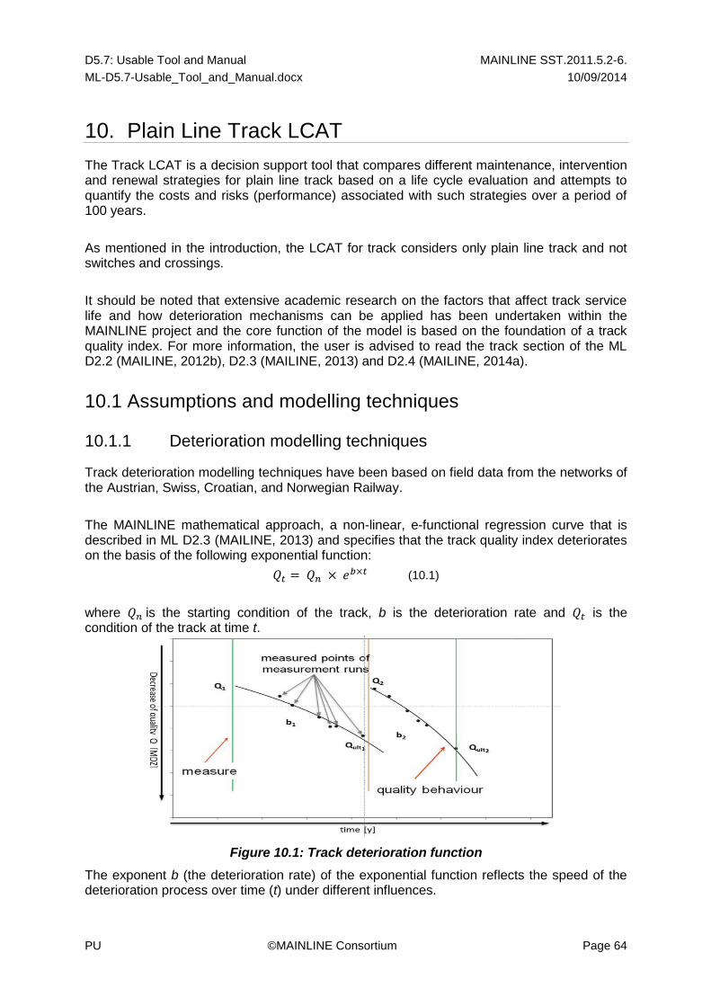
D5.7: Usable Tool and Manual MAINLINE SST.2011.5.2-6.
ML-D5.7-Usable_Tool_and_Manual.docx 10/09/2014
PU ©MAINLINE Consortium Page 64
10. Plain Line Track LCAT
The Track LCAT is a decision support tool that compares different maintenance, intervention and renewal strategies for plain line track based on a life cycle evaluation and attempts to quantify the costs and risks (performance) associated with such strategies over a period of 100 years.
As mentioned in the introduction, the LCAT for track considers only plain line track and not switches and crossings.
It should be noted that extensive academic research on the factors that affect track service life and how deterioration mechanisms can be applied has been undertaken within the MAINLINE project and the core function of the model is based on the foundation of a track quality index. For more information, the user is advised to read the track section of the ML D2.2 (MAILINE, 2012b), D2.3 (MAILINE, 2013) and D2.4 (MAILINE, 2014a).
10.1 Assumptions and modelling techniques
10.1.1 Deterioration modelling techniques
Track deterioration modelling techniques have been based on field data from the networks of the Austrian, Swiss, Croatian, and Norwegian Railway.
The MAINLINE mathematical approach, a non-linear, e-functional regression curve that is described in ML D2.3 (MAILINE, 2013) and specifies that the track quality index deteriorates on the basis of the following exponential function:
(10.1)
where is the starting condition of the track, b is the deterioration rate and is the condition of the track at time t.
Figure 10.1: Track deterioration function
The exponent b (the deterioration rate) of the exponential function reflects the speed of the deterioration process over time (t) under different influences.

D5.7: Usable Tool and Manual MAINLINE SST.2011.5.2-6.
ML-D5.7-Usable_Tool_and_Manual.docx 10/09/2014
PU ©MAINLINE Consortium Page 65
The Q and the b-values are calculated from a nonlinear regression model which consider a time series of measurement data dealing with the evaluation of track geometry (MAILINE, 2013). These measurement data are delivered by the recording car of the Austrian Federal Railways (OeBB).
Within the MAINLINE project, it was proposed to evaluate such deterioration processes for:
Three types of sleepers
Five different transport loadings
Two different track alignments
Four different lengths of radius
One operational speed (up to 130 kmph but it can be extended to up to 160 kmph)
Two drainage conditions (good/poor)
Two sub-layer conditions (good/poor)
Amongst the MAINLINE partners, it was decided that three base cases are formulated for boundary conditions of a good sub-layer quality, different transport loading and sufficient drainage facilities. Other boundary conditions are not covered within the base cases but are considered within a detailed extrapolation process for quality values, deterioration rates, and threshold values.
These three profiles coupled with a forth one, which was used under phase 2 of Task 5.5 to validate the model, were provided as examples and can be seen in Appendix 14.3 (the profiles are marked up with grey colour).
Also, it should be noted that the detailed extrapolation exercise has not been described here (the information is too extensive) but these have been tabulated and are available from the MAINLINE project team if required.
10.1.2 Further assumptions
Similar to the previous LCAT models, the Track LCAT does not have a length dimension. It can accommodate any length; the user may specify the appropriate length based on relevant cost information.
In terms of the modelled interventions, the tool is not fully flexible. It has been pre-programmed to model two intervention strategies:
(a) In-situ tamping of ballast
(b) Renew of track structure (replacement)
The user is allowed to switch on/off either of these intervention strategies to examine different options in a life cycle evaluation, but further interventions cannot be added in this prototype version of the model.
One main difference between Track LCAT and the other two models is that at the beginning of the model, the track is assumed to be brand new. This does not allow the model to start from an initial condition different from the nominal one. Table 10.3 tabulates all the main points discussed above.
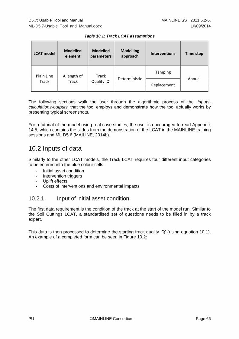
D5.7: Usable Tool and Manual MAINLINE SST.2011.5.2-6.
ML-D5.7-Usable_Tool_and_Manual.docx 10/09/2014
PU ©MAINLINE Consortium Page 66
Table 10.1: Track LCAT assumptions
LCAT model Modelled element
Modelled parameters
Modelling approach
Interventions Time step
Plain Line Track
A length of Track
Track Quality ‘Q’
Deterministic
Tamping
Annual
Replacement
The following sections walk the user through the algorithmic process of the ‘inputs-calculations-outputs’ that the tool employs and demonstrate how the tool actually works by presenting typical screenshots.
For a tutorial of the model using real case studies, the user is encouraged to read Appendix 14.5, which contains the slides from the demonstration of the LCAT in the MAINLINE training sessions and ML D5.6 (MAILINE, 2014b).
10.2 Inputs of data
Similarly to the other LCAT models, the Track LCAT requires four different input categories to be entered into the blue colour cells:
- Initial asset condition - Intervention triggers - Uplift effects - Costs of interventions and environmental impacts
10.2.1 Input of initial asset condition
The first data requirement is the condition of the track at the start of the model run. Similar to the Soil Cuttings LCAT, a standardised set of questions needs to be filled in by a track expert.
This data is then processed to determine the starting track quality ‘Q’ (using equation 10.1). An example of a completed form can be seen in Figure 10.2:

D5.7: Usable Tool and Manual MAINLINE SST.2011.5.2-6.
ML-D5.7-Usable_Tool_and_Manual.docx 10/09/2014
PU ©MAINLINE Consortium Page 67
Figure 10.2: Track LCAT – Input parameters
It should be noted that due to the lack of consistent data, the model is restricted to operational speeds to up 130 km/h, although, the user might use it up to 160 km/h. That means that the current version of the Track LCAT should not be used for high speed track sections.
10.2.2 Input of intervention triggers
Intervention strategies are listed on ‘IntvTriggers’ worksheet and the user may select/adjust the way or the scores at which interventions may be triggered. As mentioned above, there are two pre-set interventions build into the model: (a) tamping (b) replacement; the user cannot adjust these or add new ones.
Interventions can be triggered in a number of ways. Some can be programmed by the user; others rely on data which is already recorded within the model. Each intervention may be initiated by pre-programmed rules or by a score value and these ‘trigger scores’ are input on this worksheet. Alternatively, the user may specify times when the interventions are to be used (i.e. for example intervention No.1 should be applied every ten years).
Furthermore, some rules have been pre-programmed to prioritize interventions: Hence:
a. Service life: If the life of the track supersedes the pre-set service life, renewal is automatically selected.
b. Tamping: Each type of track is allowed to have some specific number of tamping interventions. If it is reached, then renewal is initialised.

D5.7: Usable Tool and Manual MAINLINE SST.2011.5.2-6.
ML-D5.7-Usable_Tool_and_Manual.docx 10/09/2014
PU ©MAINLINE Consortium Page 68
There are five switched on/off triggers and depending on user’s requirements, they can be selected or not. The first three, if selected, are pre-set by the model; the last two are set up by the user. In Figure 10.3 the first four triggers are switched on and the pre-set interventions are illustrated.
Figure 10.3: Track LCAT - intervention triggers
10.2.3 Changes caused by interventions (uplift effects)
Interventions are applied to the track in order to change its condition, improving its quality/ performance. The model allows the user to partially input what each intervention is expected to achieve; there are drop down lists from which uplift effects after intervention can be determined.
Tamping uplift effects are already pre-set in the model; the user may only decide what the uplift effects of the track renewal will achieve (uplifts in the ‘Q’ quality performance).
Tamping uplift effects are already pre-set in the model; the user may decide for the uplift effects of the renewal only. Figure 10.4 shows an example of inputting uplift effects. In this instance, when a renewal is initiated a 'Concrete with under sleeper pads' sleeper as well as 'Hard' ballast, 'Good' sub-layer and 'Good' drainage are applied.

D5.7: Usable Tool and Manual MAINLINE SST.2011.5.2-6.
ML-D5.7-Usable_Tool_and_Manual.docx 10/09/2014
PU ©MAINLINE Consortium Page 69
Figure 10.4: Track LCAT - uplift effects
10.2.4 Input of intervention costs
The costs and impacts of each intervention are summarised on the Intervention Costs worksheet below (‘IntvCosts’), but details of the costs and environmental impacts are input on a separate, more detailed worksheet for each of the two interventions called ‘IntvCost(1)’ and ‘IntvCost(2)’.
On the cost summary sheet the user may specify cost categories and budgets which may be chosen to suit the user’s own financial arrangements.
Also on the cost summary worksheet the user may identify some operational (i.e. possession costs) and environmental impacts which will arise when the intervention is executed. These may be selected by the user.
An operational or environmental impact may include a cash cost which is input here as is the cash equivalent of the operational/environmental impact (as kg of CO2 emissions). The discount rates are input on the cost summary. Different rates may be specified for cash costs and environmental equivalent costs. The selection of rates is at the discretion of the user.
The Figure 10.5 illustrates sample input figures for Intervention Costs.

D5.7: Usable Tool and Manual MAINLINE SST.2011.5.2-6.
ML-D5.7-Usable_Tool_and_Manual.docx 10/09/2014
PU ©MAINLINE Consortium Page 70
Figure 10.5: Track LCAT - Cost summary sheet
The detailed costs and environmental impact for each intervention are shown in individual costing sheets, illustrated in Figures 10.6 and 10.7:

D5.7: Usable Tool and Manual MAINLINE SST.2011.5.2-6.
ML-D5.7-Usable_Tool_and_Manual.docx 10/09/2014
PU ©MAINLINE Consortium Page 71
Figure 10.6: Track LCAT - Intervention cost details
The user may specify detailed financial costs associated with the particular intervention, split into different categories (i.e. Labour, Plant, Materials, Tax) as well as greenhouse gases emission, measured by their carbon dioxide equivalent mass (kg CO2e) unit. It is worthwhile to mention that the environmental impacts can be measured by three different environmental effects. Carbon emission (CO2 greenhouse gases emission) is the first pre-set environmental measure, however, the user may specify up to three different ones (i.e. waste, water pollution etc.). For example, the ML D5.2 (MAILINE, 2012c) pointed out that the next most relevant impacts after the greenhouse gases emission is waste. The sum of these CO2 emissions is translated into cash using user’s pre-set cash equivalent factor.

D5.7: Usable Tool and Manual MAINLINE SST.2011.5.2-6.
ML-D5.7-Usable_Tool_and_Manual.docx 10/09/2014
PU ©MAINLINE Consortium Page 72
Assessment of environmental impacts
The environmental impact of each item on the cost details sheet is drawn from a reference list of Impacts which is common to all models and all interventions.
This library of environmental impacts is a result of a detailed environmental analysis exercise within the MAINLINE project and includes state of the art research (for more information, the user is advised to read the ML D5.2 document (MAILINE, 2012c) which focuses on this research). This library may be used to build up the environmental impacts for any intervention. The user has the choice to add further environmental impacts according to their standards and conditions.
A sample from the reference list is given below:
Figure 10.7: Track LCAT - Sample of environmental impact reference data
MAINLINE Soil Cutting Model
Environment Impact of Construction Activity
version 3
Users may amend this data and add more data if necessary
NOTES:
1 These impact values will be used to build-up the environmental impact of the interventions employed in asset life-cycles.
2 The data will be applicable across Europe. If it is specific to a certain country, this is noted.
3 The impacts of materials are shown as from cradle-to-factorygate.
4 The impacts of equipment and transport will include only fuel usage (excluding the manufacture of the equipment or vehicle).
5 Different types and sizes of equipment should be shown on separate lines, where appropriate.
6 Different types of paints and coatings should be shown on separate lines, where appropriate.
Brid
ges
Cu
ttin
gs
Track
Tu
nn
els
Group ItemUnit of
usage
CO2e
[kg/unit of
usage]
Basis of impact estimationNote on impact
assessmentSources of Impact data
• Materials Ballast m3 50.72 0.0317 kgCO2e/kg x density 1600 kg/m3 (assumed crushed rock 16/32
mm)
Database of GaBi 6 (PE International)
• Equipment Ballast stoneblower km 418.0000 data from research paper (see reference column L) Milford, R & Allwood, J. (2010) "Assessing the CO2 impact of
current and future rail track in the UK", Transportation
Research Part D 15, pp. 61-72.
• Equipment Ballast tamper km 153.00 data from research paper (see reference column L) Milford, R & Allwood, J. (2010) "Assessing the CO2 impact of
current and future rail track in the UK", Transportation
Research Part D 15, pp. 61-72.
• • Materials Brickwork - single skin brick m2 44.88 0.22 kg CO2e/kg x2000kg/m3 x 0.102m brick thickness. Assumed clay brick
density, 2000kg/m3.
Ecoinvent database
• • • • Equipment Chainsaw (5) hr 3.35 Power chainsaw with catalytic converter with assumed 1.25kg petrol usage
per hour
Database of GaBi 6 (PE International)
• • • • Materials Concrete, mass insitu m3 221.26 0..0962 kgCO2e/kg x density 2300kg/m3. Assuming use of ready-mix
concrete C20/25.
Database of GaBi 6 (PE International)
• • • • Materials Concrete, precast m3 333.60 0.139 kg CO2e/kg x 2400 kg/m3. Assuming concrete type C20/25 and
minimum reinforcement share of 0.5%.
Database of GaBi 6 (PE international)
• • • Equipment Crane, mobile (5) hr 15.80 3.16 kg CO2e/litre x 5 litre/hour. Assuming 15t wheeled crane and diesel
consumption 5 litre/hour. (U.K. data)
U.K. Environment Agency and CESMM3
• Equipment Crane, static (5) hr 15.80 Assuming similar to mobile crane.
• • • • Materials Diesel fuel l 2.68
• Materials Epoxy resin kg 8.2800 Plastic Europe
• • • • Equipment Excavator (5) t 0.55 Assuming 100kW excavator, diesel driven and for excavating 1 tonne of
material
Database of GaBi 6 (PE International)
• Materials Geo-textile m2 0.96 2,13 kgCO2e/kg x density 903 kg/m3 x thickness 0,0005 m (assuming
polyethylene film (PE-HD) with polypropylene (PP) fleece for sealing)
Database of GaBi 6 (PE International)
• Materials Glass fibre reinforced plastic kg 8.7600 Assuming GFRP production with injection moulding glass fibre method. Ecoinvent database
• • • • Materials Granular fill m3 11.200 0.0045 kgCO2e/kg x 2240 kg/m3 . Assumed sand and gravel (2/32mm)
density, 2240 kg/m3.
Database of GaBi 6 (PE international)
Model
back to: Flowchart

D5.7: Usable Tool and Manual MAINLINE SST.2011.5.2-6.
ML-D5.7-Usable_Tool_and_Manual.docx 10/09/2014
PU ©MAINLINE Consortium Page 73
10.3 Calculations and inner workings
The underlying calculations of the model take place in three working sheets which are not used for any input or output. They are described briefly below but their detailed operation is beyond the scope of this user manual. The form and workings of these sheets are necessarily specific to track model and may be different between LCAT models.
10.3.1 Deterioration Rates
On the ‘DetRates’ sheet the input data about the asset initial condition are pre-processed into the calculation of the deterioration data over the next 100 years before being passed to the ‘Projection' sheet.
10.3.2 Projection
This combines the deterioration data from the ‘DetRates’ sheet, the initial condition of the asset and the intervention triggers and uplift effects to generate the projection of the intervention plan required and the track quality condition over the 100-years period.
10.3.3 Results
This is a sorting area where data from the projection is collated with intervention cost data to provide the source of the data for the output sheets. The data here is arranged in a standard format to match the output requirements.
10.4 Outputs of data
As already described, the output sheets for all the LCATs are in broadly the same format. The principal output sheets for the Track LCAT, coloured purple in the model, are
- Summary - Output Financial - Output Environmental - Output Operations - Output Condition
which are escribed in more detail below and illustrated in Figures 10.8 To 10.12
10.4.1 Output Summary (Figure 10.8)
This worksheet is the main output of the model which concludes all the information for the user. It gives an overview of the interventions employed, the overall costs and impacts, and summary charts of the projected cash equivalent expenditure and asset condition.
10.4.2 Output Financial (Figure 10.9)
This worksheet focuses on the financial costs associated with the intervention plan of the asset over the next 100 years.

D5.7: Usable Tool and Manual MAINLINE SST.2011.5.2-6.
ML-D5.7-Usable_Tool_and_Manual.docx 10/09/2014
PU ©MAINLINE Consortium Page 74
It gives more details of the cash flow in terms of financial costs as well as cash equivalents of the environmental and operational impacts. These results can be shown with or without discounting over the 100-year period.
10.4.3 Output Environmental (Figure 10.10)
This worksheet summarises the environmental aspects of the intervention plan of the asset over the projected time of 100 years.
It shows the summary of the environmental impacts as CO2 emissions resulting from each of the interventions used and the total impact in each modelling period.
10.4.4 Output Operations (Figure 10.11)
This worksheet tabulates the operational impacts (i.e. possession costs) and the loss of revenue due to the required intervention plan over the next 100 years.
It shows the summary of the operational impacts resulting from each of the interventions used and the total impact in each modelling period.
Furthermore, within LCAT for track, typical data from the Austrian network, related to costs from operational impacts, have been gathered and published and can be provided under request as guideline for the user.
10.4.5 Output Condition (Figure 10.12)
The last output worksheet concentrates on the service condition (performance) of the asset. It shows the projection of the various the track quality in the start and end time of a year over time.

D5.7: Usable Tool and Manual MAINLINE SST.2011.5.2-6.
ML-D5.7-Usable_Tool_and_Manual.docx 10/09/2014
PU ©MAINLINE Consortium Page 75
Figure 10.8: Track LCAT - Output summary

D5.7: Usable Tool and Manual MAINLINE SST.2011.5.2-6.
ML-D5.7-Usable_Tool_and_Manual.docx 10/09/2014
PU ©MAINLINE Consortium Page 76
Figure 10.9: Track LCAT - Financial output
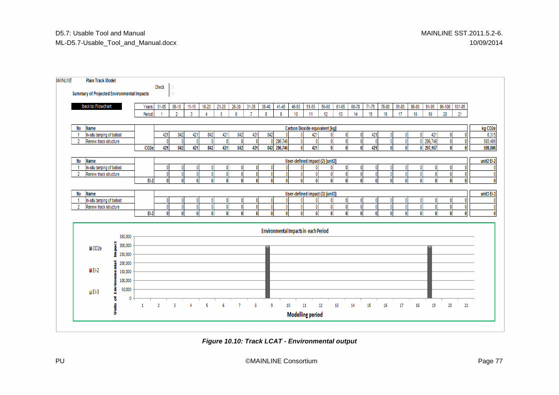
D5.7: Usable Tool and Manual MAINLINE SST.2011.5.2-6.
ML-D5.7-Usable_Tool_and_Manual.docx 10/09/2014
PU ©MAINLINE Consortium Page 77
Figure 10.10: Track LCAT - Environmental output

D5.7: Usable Tool and Manual MAINLINE SST.2011.5.2-6.
ML-D5.7-Usable_Tool_and_Manual.docx 10/09/2014
PU ©MAINLINE Consortium Page 78
Figure 10.11: Track LCAT - Operational output

D5.7: Usable Tool and Manual MAINLINE SST.2011.5.2-6.
ML-D5.7-Usable_Tool_and_Manual.docx 10/09/2014
PU ©MAINLINE Consortium Page 79
Figure 10.12: Track LCAT - Condition output

D5.7: Usable Tool and Manual MAINLINE SST.2011.5.2-6.
ML-D5.7-Usable_Tool_and_Manual.docx 10/09/2014
PU ©MAINLINE Consortium Page 80
10.4.6 Summary of outputs
The upper part of Figure 10.8 shows the intervention schedule followed by the cash equivalents in each 5 year period.
The lower part of Figure 10.8 shows the projected track quality ‘Q’ at the start and end of each period through the planned 100 years. In this example, it is seen that a major intervention (renewal of track) on period 9, results in a restoration of the track condition
In Error! Reference source not found. Figure 10.9, the financial costs of the intervention lan of Figure 10.8 can be demonstrated in a discount rate (the rate is specified by the user), which is the preferred measure for comparison of different maintenance strategies.
Figures 10.10, 10.11 and 10.12 provide more detailed information about the operational and environmental impacts of the proposed intervention plan and how these are translated into cash as well as the performance of the cutting through time.
Last but not least, for a validation of the model with real case studies, the user may reference the Track section of ML D5.6 (MAILINE, 2014b).
10.4.7 Interpretation of the results
To conclude with, the LCAT for track focuses on a prediction of the track’s technical service life (TSL) under different boundary conditions (input parameters).
These boundary conditions are:
- ballast quality - traffic load - radius - sleeper type - drainage condition - sub-layer condition
All basic information about track behaviour are derived from real track data covering the entire core track infrastructure of Austria, Switzerland, Croatia and parts of Norway.
This technical service life allows running trains at the full speed of the section; speed restrictions in order to increase service life are not taken into account as they are uneconomical for main lines. Thus, this service life is the longest service life possible, without any operational restriction.
The status of components must be analysed additionally as well as all safety relevant information.
If the initial quality was poor and/or maintenance was not executed sufficiently the technical service life cannot be reached.

D5.7: Usable Tool and Manual MAINLINE SST.2011.5.2-6.
ML-D5.7-Usable_Tool_and_Manual.docx 10/09/2014
PU ©MAINLINE Consortium Page 81
Due to these limitations, LCAT for track is a tool to support track engineers in focusing the decision making on the entire service life. This should lead to a more sustainable track.
However, as LCAT for track is focusing on the technical service life itself, it does not consider any safety critical situations or specific local conditions It is designed to deliver information to define general track strategies.

D5.7: Usable Tool and Manual MAINLINE SST.2011.5.2-6.
ML-D5.7-Usable_Tool_and_Manual.docx 10/09/2014
PU ©MAINLINE Consortium Page 82
11. Limitations of LCATs and Future Work
The LCATs provide a useful tool for evaluating whole life cost of the different assets. However, as with all models, there are limitations for their use.
One limitation of the MAINLINE LCATs is that they do not include an optimisation engine which examines different scenarios (for a specific set of inputs) and returns the optimum. Instead, given a set of input parameters they process the data and return the first solution that is triggered by the predefined intervention strategies. An LCAT will need to be run a number of times with different parameters to determine the optimum solution.
The MAINLINE LCATs also employ deterministic deterioration modelling techniques, which will always lead to the same outcome given the same set of inputs whilst a probabilistic process would incorporate uncertainty in the inputs, which in turn leads to a set of possible outcomes occurring; however probabilistic deterioration models are not currently available for the assets considered by the MAINLINE project.
There are benefits and limitations to each of these deterioration modelling approaches, which pose a challenge in selecting the most appropriate technique. In practice many of the processes that are important in the subject of asset management involve risk and it is usually difficult to accurately describe them with a deterministic forecast without taking into account the inherent uncertainty of the behaviour of the assets.
After the completion of the MAINLINE project, further research and development work could be carried out by others in the following areas:
1. Collation of data from other asset types to allow for the creation degradation rates of other materials and assets.
2. Collation of further data for the existing LCAT models to give greater validation of deterioration rates.
3. Creation of LCAT models for different assets based on the new data. 4. Continuous updates to the existing LCAT models based on new data and user
feedback. 5. Creation of a ‘combined LCAT’ to consider holistic risk and whole life costing for a
system approach rather than by individual assets. 6. Greater number of environmental factors within the LCAT models including ‘noise’. 7. Investigate the feasibility of adding a probabilistic approach into the LCAT models. 8. Create an optimisation tool within the LCAT. 9. Investigate the incorporation of fatigue modelling within the Metallic Bridges LCAT.

D5.7: Usable Tool and Manual MAINLINE SST.2011.5.2-6.
ML-D5.7-Usable_Tool_and_Manual.docx 10/09/2014
PU ©MAINLINE Consortium Page 83
12. Conclusions
This document is the user manual for the LCAT models developed within the MAINLINE project. Despite the best efforts of the MAINLINE partners, the data required for the development of deterioration profiles for all the asset types originally proposed has not been forthcoming, which has limited the development of deterioration profiles to, and hence LCATs for:
Metallic bridges Soil cuttings Plain line track
which together represent a substantial proportion of the assets of European railway administrations.
The method of modelling within each of these LCATs is bespoke, detailed and the tools have been individually custom-designed based on the engineering behaviour of the asset types. They provide what are believed to be the first decision support models to combine environmental and economic impacts and, in the case of Metallic Bridges LCAT, to also combine condition and capability considerations.

D5.7: Usable Tool and Manual MAINLINE SST.2011.5.2-6.
ML-D5.7-Usable_Tool_and_Manual.docx 10/09/2014
PU ©MAINLINE Consortium Page 84
13. References
EN ISO 9223 (2012), Corrosion of metals and alloys - Corrosivity of atmospheres - Classification, determination and estimation, 2012.
ISO 14040 (2006), Environmental management -- Life cycle assessment -- Principles and framework.
ISO 55000 (2014), Asset Management – Overview, Principles and Terminology of Asset Management.
ISO 55001 (2014), Asset Management – Management system requirements.
ISO 55002 (2014), Asset Management – Guidelines for the application of ISO 55001.
MAINLINE (2012a), ML D2.1 – Degradation and performance specification for selected assets.
MAINLINE (2012b), ML D2.2 – Degradation and intervention modelling techniques.
MAINLINE (2013), ML D2.3 – Time-variant performance profiles for LCC and LCA.
MAINLINE (2014a), ML D2.4 – Field validation of performance profiles.
MAINLINE (2012c), ML D5.2 – Assessment of environmental performance tools and methods.
MAINLINE (2014b), ML D 5.6 – Validation of LCAT models.

D5.7: Usable Tool and Manual MAINLINE SST.2011.5.2-6.
ML-D5.7-Usable_Tool_and_Manual.docx 10/09/2014
PU ©MAINLINE Consortium Page 85
14. Appendices
14.1 Track LCAT: Performance profiles
14.1.1 Performance profile I
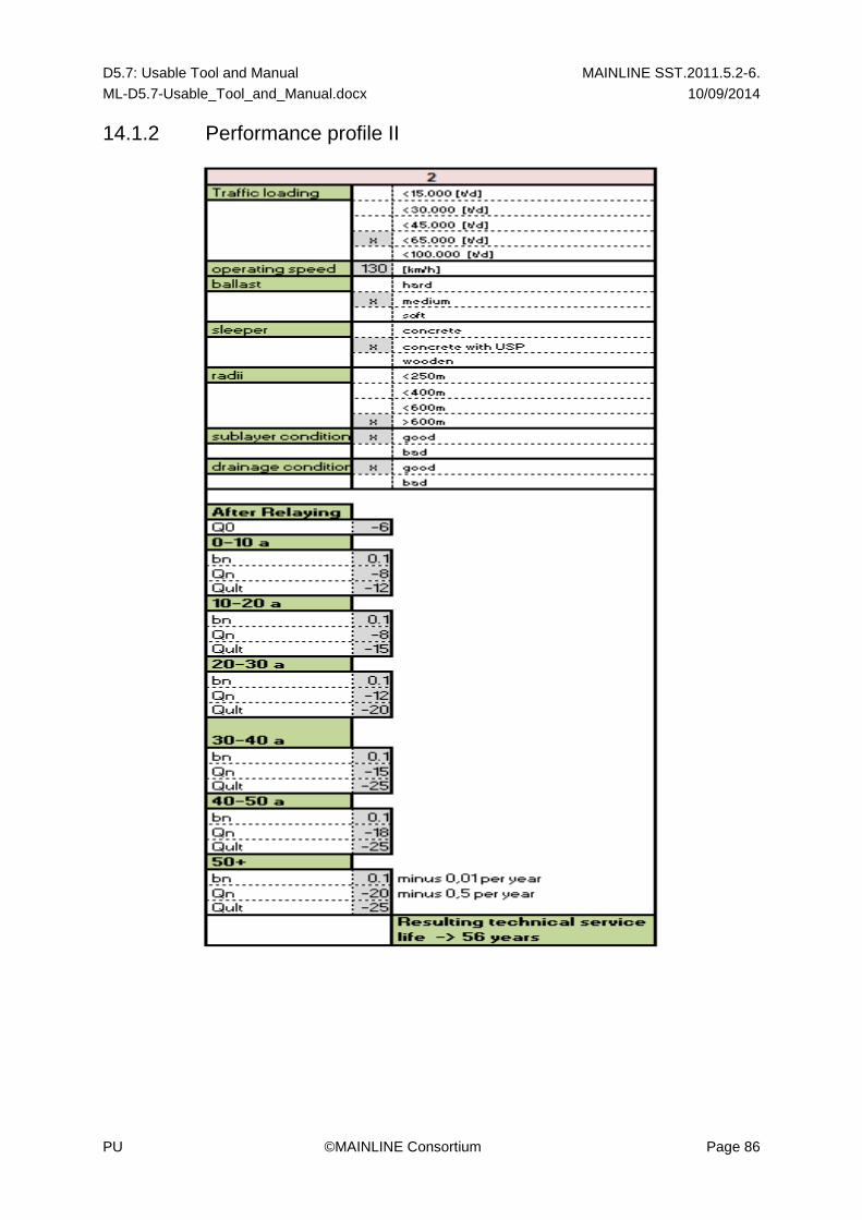
D5.7: Usable Tool and Manual MAINLINE SST.2011.5.2-6.
ML-D5.7-Usable_Tool_and_Manual.docx 10/09/2014
PU ©MAINLINE Consortium Page 86
14.1.2 Performance profile II

D5.7: Usable Tool and Manual MAINLINE SST.2011.5.2-6.
ML-D5.7-Usable_Tool_and_Manual.docx 10/09/2014
PU ©MAINLINE Consortium Page 87
14.1.3 Performance profile III

D5.7: Usable Tool and Manual MAINLINE SST.2011.5.2-6.
ML-D5.7-Usable_Tool_and_Manual.docx 10/09/2014
PU ©MAINLINE Consortium Page 88
14.2 VBA Macros for the Bridges LCAT
14.2.1 When coating systems data does not exist

D5.7: Usable Tool and Manual MAINLINE SST.2011.5.2-6.
ML-D5.7-Usable_Tool_and_Manual.docx 10/09/2014
PU ©MAINLINE Consortium Page 89
14.2.2 When coating systems data exists

D5.7: Usable Tool and Manual MAINLINE SST.2011.5.2-6.
ML-D5.7-Usable_Tool_and_Manual.docx 10/09/2014
PU ©MAINLINE Consortium Page 90
14.3 LCAT for Soil Cuttings – Tutorial (Slides from LCAT Training session)

D5.7: Usable Tool and Manual MAINLINE SST.2011.5.2-6.
ML-D5.7-Usable_Tool_and_Manual.docx 10/09/2014
PU ©MAINLINE Consortium Page 91
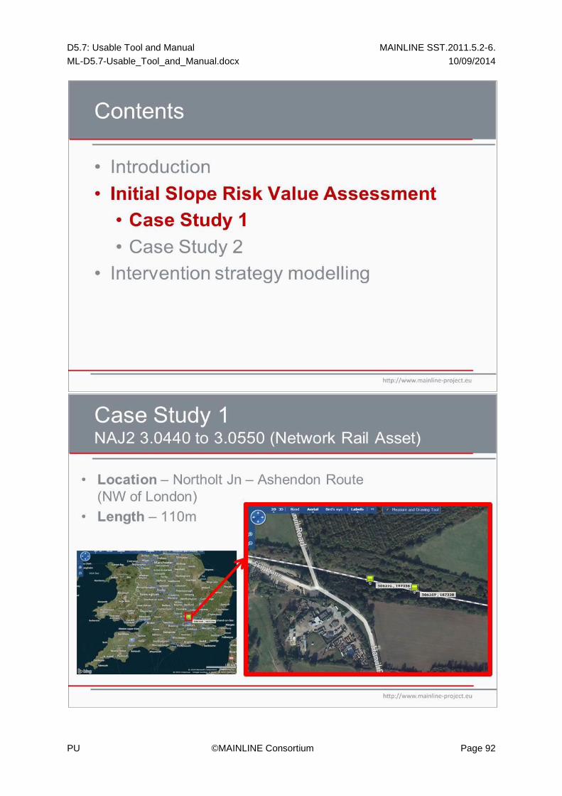
D5.7: Usable Tool and Manual MAINLINE SST.2011.5.2-6.
ML-D5.7-Usable_Tool_and_Manual.docx 10/09/2014
PU ©MAINLINE Consortium Page 92

D5.7: Usable Tool and Manual MAINLINE SST.2011.5.2-6.
ML-D5.7-Usable_Tool_and_Manual.docx 10/09/2014
PU ©MAINLINE Consortium Page 93

D5.7: Usable Tool and Manual MAINLINE SST.2011.5.2-6.
ML-D5.7-Usable_Tool_and_Manual.docx 10/09/2014
PU ©MAINLINE Consortium Page 94

D5.7: Usable Tool and Manual MAINLINE SST.2011.5.2-6.
ML-D5.7-Usable_Tool_and_Manual.docx 10/09/2014
PU ©MAINLINE Consortium Page 95

D5.7: Usable Tool and Manual MAINLINE SST.2011.5.2-6.
ML-D5.7-Usable_Tool_and_Manual.docx 10/09/2014
PU ©MAINLINE Consortium Page 96

D5.7: Usable Tool and Manual MAINLINE SST.2011.5.2-6.
ML-D5.7-Usable_Tool_and_Manual.docx 10/09/2014
PU ©MAINLINE Consortium Page 97

D5.7: Usable Tool and Manual MAINLINE SST.2011.5.2-6.
ML-D5.7-Usable_Tool_and_Manual.docx 10/09/2014
PU ©MAINLINE Consortium Page 98

D5.7: Usable Tool and Manual MAINLINE SST.2011.5.2-6.
ML-D5.7-Usable_Tool_and_Manual.docx 10/09/2014
PU ©MAINLINE Consortium Page 99

D5.7: Usable Tool and Manual MAINLINE SST.2011.5.2-6.
ML-D5.7-Usable_Tool_and_Manual.docx 10/09/2014
PU ©MAINLINE Consortium Page 100
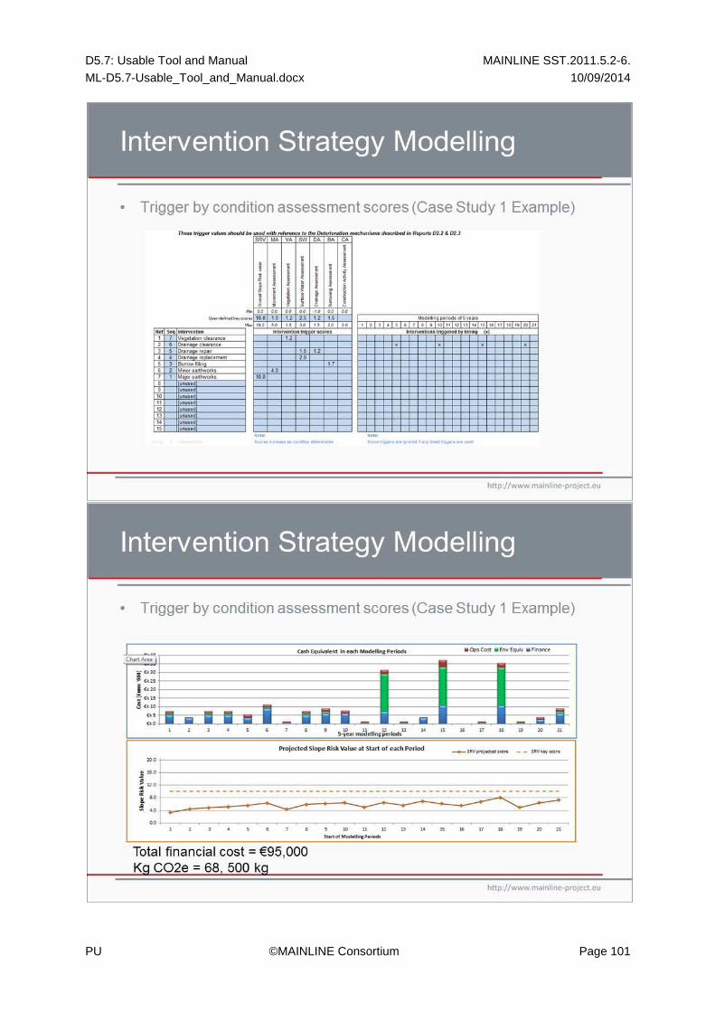
D5.7: Usable Tool and Manual MAINLINE SST.2011.5.2-6.
ML-D5.7-Usable_Tool_and_Manual.docx 10/09/2014
PU ©MAINLINE Consortium Page 101

D5.7: Usable Tool and Manual MAINLINE SST.2011.5.2-6.
ML-D5.7-Usable_Tool_and_Manual.docx 10/09/2014
PU ©MAINLINE Consortium Page 102

D5.7: Usable Tool and Manual MAINLINE SST.2011.5.2-6.
ML-D5.7-Usable_Tool_and_Manual.docx 10/09/2014
PU ©MAINLINE Consortium Page 103
14.4 LCAT for Bridges – Tutorial (Slides from LCAT Training session)

D5.7: Usable Tool and Manual MAINLINE SST.2011.5.2-6.
ML-D5.7-Usable_Tool_and_Manual.docx 10/09/2014
PU ©MAINLINE Consortium Page 104

D5.7: Usable Tool and Manual MAINLINE SST.2011.5.2-6.
ML-D5.7-Usable_Tool_and_Manual.docx 10/09/2014
PU ©MAINLINE Consortium Page 105

D5.7: Usable Tool and Manual MAINLINE SST.2011.5.2-6.
ML-D5.7-Usable_Tool_and_Manual.docx 10/09/2014
PU ©MAINLINE Consortium Page 106

D5.7: Usable Tool and Manual MAINLINE SST.2011.5.2-6.
ML-D5.7-Usable_Tool_and_Manual.docx 10/09/2014
PU ©MAINLINE Consortium Page 107

D5.7: Usable Tool and Manual MAINLINE SST.2011.5.2-6.
ML-D5.7-Usable_Tool_and_Manual.docx 10/09/2014
PU ©MAINLINE Consortium Page 108

D5.7: Usable Tool and Manual MAINLINE SST.2011.5.2-6.
ML-D5.7-Usable_Tool_and_Manual.docx 10/09/2014
PU ©MAINLINE Consortium Page 109
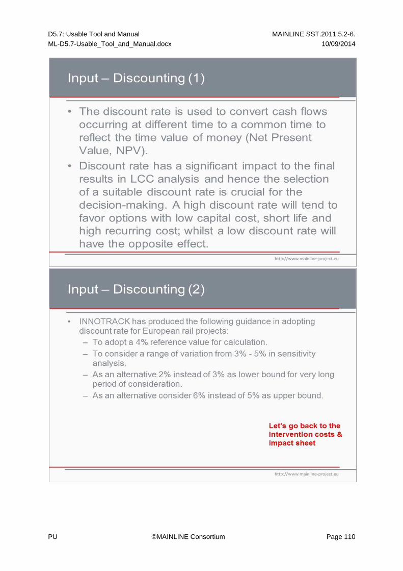
D5.7: Usable Tool and Manual MAINLINE SST.2011.5.2-6.
ML-D5.7-Usable_Tool_and_Manual.docx 10/09/2014
PU ©MAINLINE Consortium Page 110
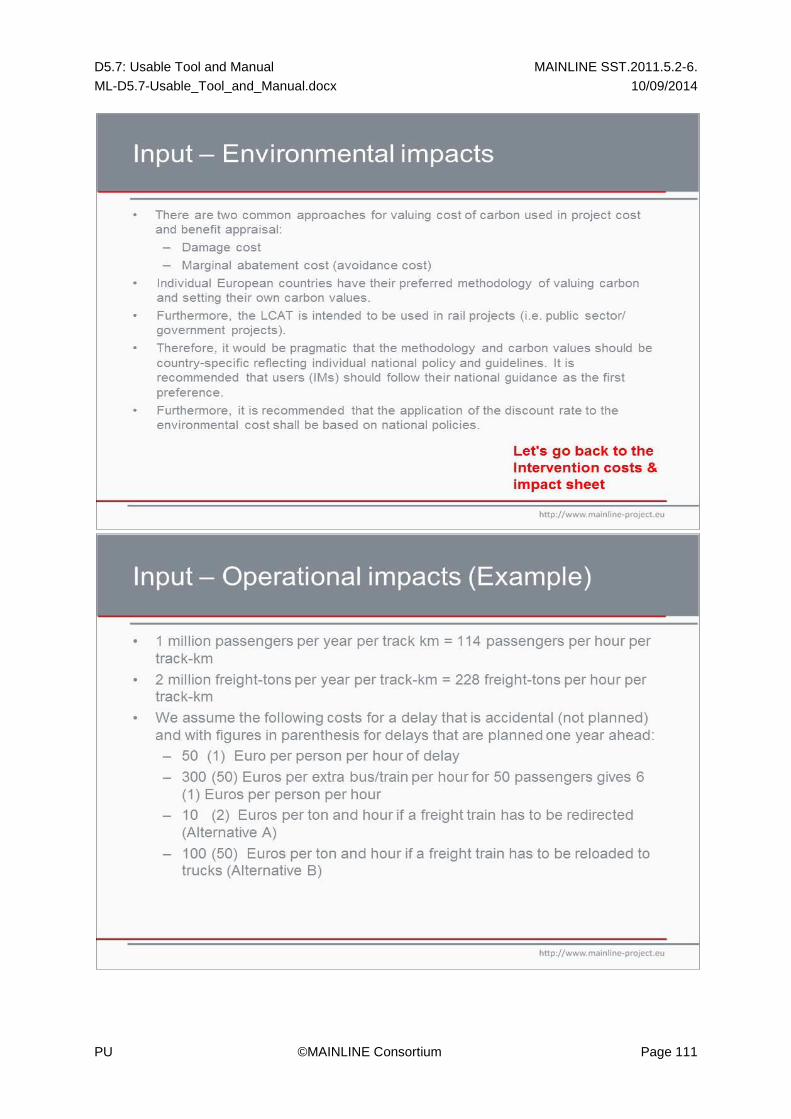
D5.7: Usable Tool and Manual MAINLINE SST.2011.5.2-6.
ML-D5.7-Usable_Tool_and_Manual.docx 10/09/2014
PU ©MAINLINE Consortium Page 111

D5.7: Usable Tool and Manual MAINLINE SST.2011.5.2-6.
ML-D5.7-Usable_Tool_and_Manual.docx 10/09/2014
PU ©MAINLINE Consortium Page 112

D5.7: Usable Tool and Manual MAINLINE SST.2011.5.2-6.
ML-D5.7-Usable_Tool_and_Manual.docx 10/09/2014
PU ©MAINLINE Consortium Page 113

D5.7: Usable Tool and Manual MAINLINE SST.2011.5.2-6.
ML-D5.7-Usable_Tool_and_Manual.docx 10/09/2014
PU ©MAINLINE Consortium Page 114
D5.7: Usable Tool and Manual MAINLINE SST.2011.5.2-6.
ML-D5.7-Usable_Tool_and_Manual.docx 10/09/2014
PU ©MAINLINE Consortium Page 115
14.5 LCAT for Track – Tutorial (Slides from the LCAT Training session)

D5.7: Usable Tool and Manual MAINLINE SST.2011.5.2-6.
ML-D5.7-Usable_Tool_and_Manual.docx 10/09/2014
PU ©MAINLINE Consortium Page 116
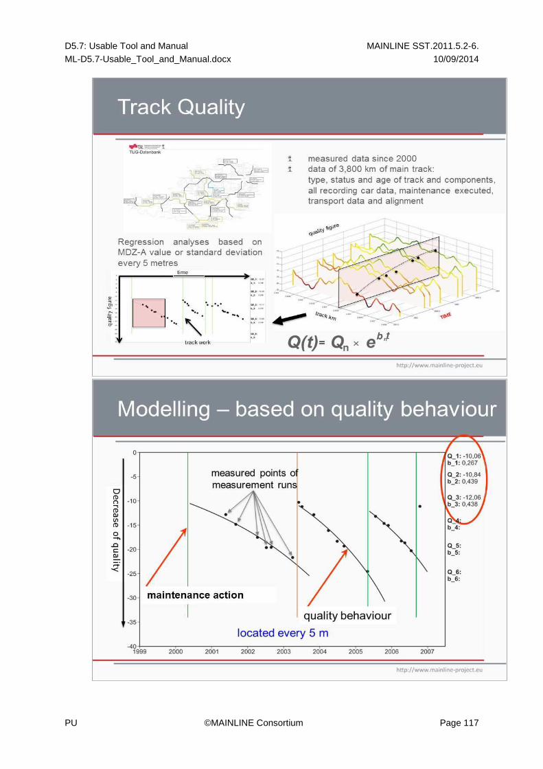
D5.7: Usable Tool and Manual MAINLINE SST.2011.5.2-6.
ML-D5.7-Usable_Tool_and_Manual.docx 10/09/2014
PU ©MAINLINE Consortium Page 117

D5.7: Usable Tool and Manual MAINLINE SST.2011.5.2-6.
ML-D5.7-Usable_Tool_and_Manual.docx 10/09/2014
PU ©MAINLINE Consortium Page 118

D5.7: Usable Tool and Manual MAINLINE SST.2011.5.2-6.
ML-D5.7-Usable_Tool_and_Manual.docx 10/09/2014
PU ©MAINLINE Consortium Page 119

D5.7: Usable Tool and Manual MAINLINE SST.2011.5.2-6.
ML-D5.7-Usable_Tool_and_Manual.docx 10/09/2014
PU ©MAINLINE Consortium Page 120

D5.7: Usable Tool and Manual MAINLINE SST.2011.5.2-6.
ML-D5.7-Usable_Tool_and_Manual.docx 10/09/2014
PU ©MAINLINE Consortium Page 121

D5.7: Usable Tool and Manual MAINLINE SST.2011.5.2-6.
ML-D5.7-Usable_Tool_and_Manual.docx 10/09/2014
PU ©MAINLINE Consortium Page 122

D5.7: Usable Tool and Manual MAINLINE SST.2011.5.2-6.
ML-D5.7-Usable_Tool_and_Manual.docx 10/09/2014
PU ©MAINLINE Consortium Page 123

D5.7: Usable Tool and Manual MAINLINE SST.2011.5.2-6.
ML-D5.7-Usable_Tool_and_Manual.docx 10/09/2014
PU ©MAINLINE Consortium Page 124

D5.7: Usable Tool and Manual MAINLINE SST.2011.5.2-6.
ML-D5.7-Usable_Tool_and_Manual.docx 10/09/2014
PU ©MAINLINE Consortium Page 125