Mankiw 5/e Chapter 12: Agg Demand in the Open Economycameron.edu/~abduls/econ5213/Pdf/ch12.pdfCHAPTER 12 Aggregate Demand in the Open Economy slide 1 Learning objectives The Mundell-Fleming

macroeconomicsfifth edition

N. Gregory Mankiw

PowerPoint® Slides by Ron Cronovichm

acro

© 2002 Worth Publishers, all rights reserved

CHAPTER TWELVE

Aggregate Demand in the Open Economy

CHAPTER 12CHAPTER 12 Aggregate Demand in the Open EconomyAggregate Demand in the Open Economy slide 1

Learning objectivesLearning objectivesThe Mundell-Fleming model: IS-LM for the small open economy

Causes and effects of interest rate differentials

Arguments for fixed vs. floating exchange rates

The aggregate demand curve for the small open economy


The The MundellMundell--Fleming ModelFleming ModelKey assumption: Small open economy with perfect capital mobility.

r = r*

Goods market equilibrium---the IS* curve:

( ) ( ) ( )*Y C Y T I r G NX e= − + + +

where e = nominal exchange rate

= foreign currency per unit of domestic currency


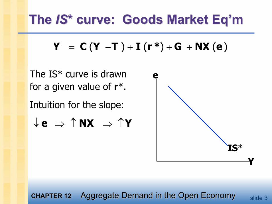
The The IS*IS* curve: Goods Market curve: Goods Market Eq’mEq’m

( ) ( ) ( )*Y C Y T I r G NX e= − + + +

The IS* curve is drawn for a given value of r*.

Intuition for the slope:

e NX Y↓ ⇒ ↑ ⇒ ↑

Y

e

IS*


The The LM*LM* curve: Money Market curve: Money Market Eq’mEq’m

( , )*M P L r Y=

The LM* curve

is drawn for a given value of r*is vertical because:given r*, there is only one value of Ythat equates money demand with supply, regardless of e.

Y

e LM*


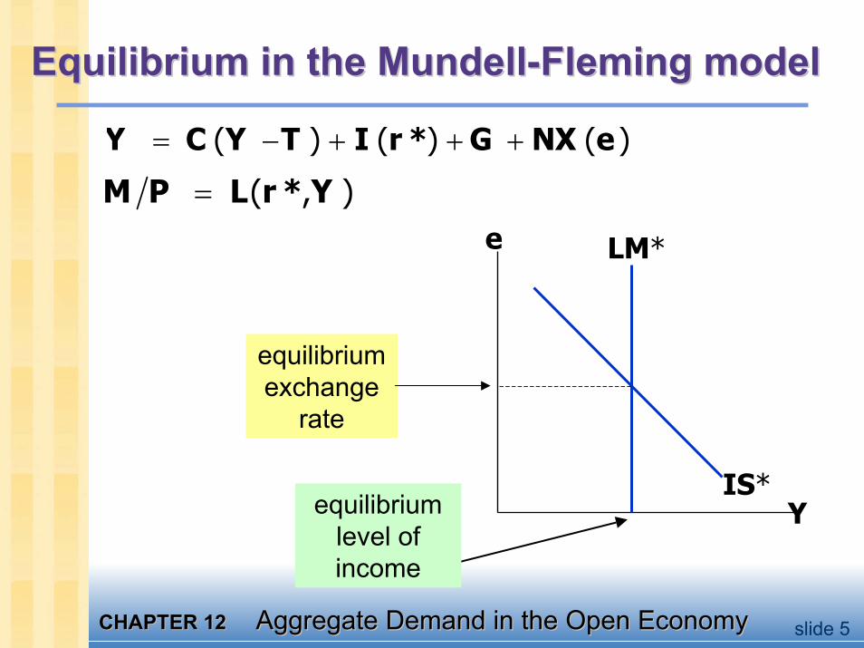
Equilibrium in the Equilibrium in the MundellMundell--Fleming modelFleming model

( ) ( ) ( )*Y C Y T I r G NX e= − + + +

( , )*M P L r Y=

Y

e LM*

IS*

equilibriumexchange

rate

equilibriumlevel ofincome


Floating & fixed exchange ratesFloating & fixed exchange rates

In a system of floating exchange rates, e is allowed to fluctuate in response to changing economic conditions.

In contrast, under fixed exchange rates, the central bank trades domestic for foreign currency at a predetermined price.

We now consider fiscal, monetary, and trade policy: first in a floating exchange rate system, then in a fixed exchange rate system.


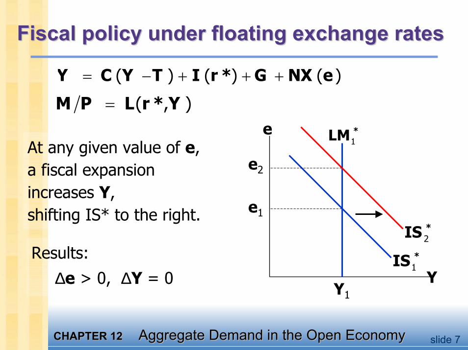
Fiscal policy under floating exchange ratesFiscal policy under floating exchange rates

( ) ( ) ( )*Y C Y T I r G NX e= − + + +

( , )*M P L r Y=

Y

e

Y1

e1

1*LM

1*IS

2*IS

e2

At any given value of e, a fiscal expansion increases Y, shifting IS* to the right.

Results: ∆e > 0, ∆Y = 0


Lessons about fiscal policyLessons about fiscal policy

In a small open economy with perfect capital mobility, fiscal policy is utterly incapable of affecting real GDP.

“Crowding out”• closed economy:

Fiscal policy crowds out investment by causing the interest rate to rise.

• small open economy:Fiscal policy crowds out net exports by causing the exchange rate to appreciate.


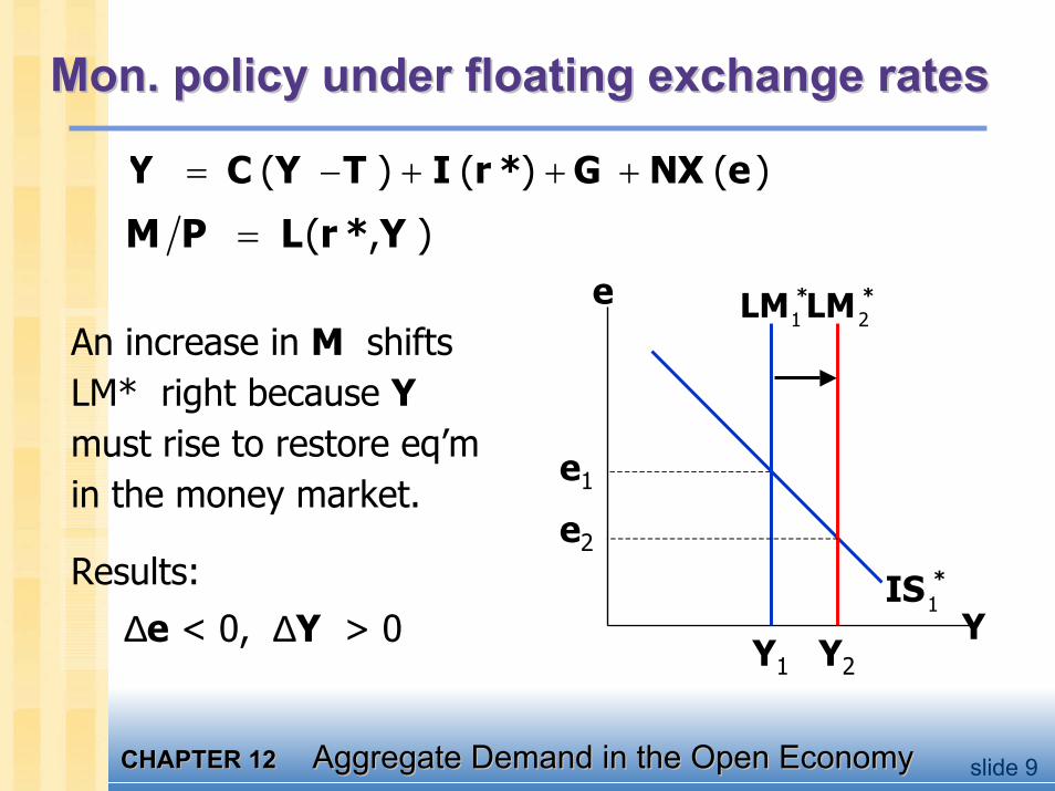
Mon. policy under floating exchange ratesMon. policy under floating exchange rates

( ) ( ) ( )*Y C Y T I r G NX e= − + + +

( , )*M P L r Y=

Y

e

e1

Y1

1*LM

1*IS

Y2

2*LM

e2

An increase in M shifts LM* right because Ymust rise to restore eq’m in the money market.

Results: ∆e < 0, ∆Y > 0


Lessons about monetary policyLessons about monetary policy

Monetary policy affects output by affecting one (or more) of the components of aggregate demand:

closed economy: ↑M ⇒ ↓ r ⇒ ↑ I ⇒ ↑ Ysmall open economy: ↑M ⇒ ↓ e ⇒ ↑ NX ⇒ ↑ Y

Expansionary mon. policy does not raise world aggregate demand, it shifts demand from foreign to domestic products. Thus, the increases in income and employment at home come at the expense of losses abroad.


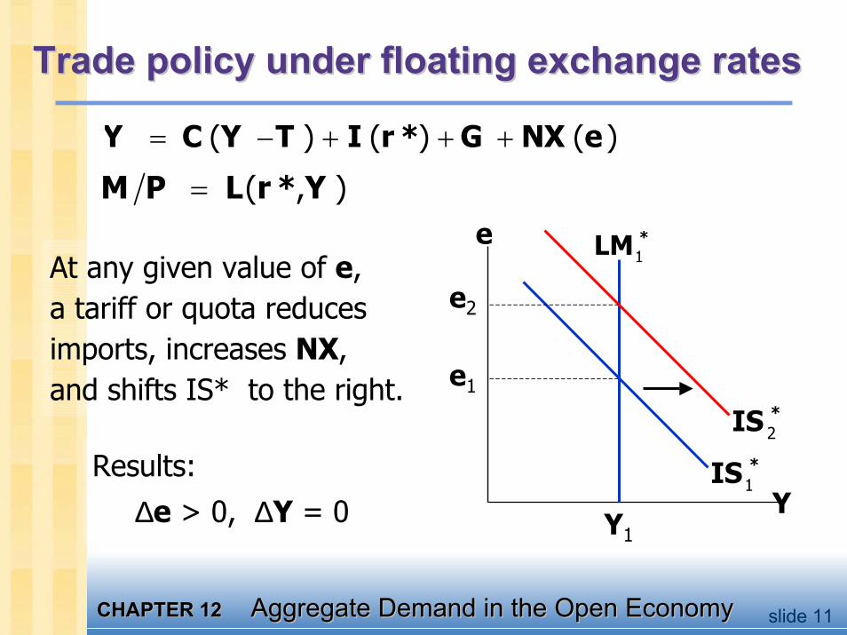
Trade policy under floating exchange ratesTrade policy under floating exchange rates

( ) ( ) ( )*Y C Y T I r G NX e= − + + +

( , )*M P L r Y=

Y

e

e1

Y1

1*LM

1*IS

2*IS

e2

At any given value of e, a tariff or quota reduces imports, increases NX, and shifts IS* to the right.

Results: ∆e > 0, ∆Y = 0


Lessons about trade policyLessons about trade policyImport restrictions cannot reduce a trade deficit.

Even though NX is unchanged, there is less trade:– the trade restriction reduces imports – the exchange rate appreciation reduces exports

Less trade means fewer ‘gains from trade.’

Import restrictions on specific products save jobs in the domestic industries that produce those products, but destroy jobs in export-producing sectors. Hence, import restrictions fail to increase total employment. Worse yet, import restrictions create “sectoralshifts,” which cause frictional unemployment.


Fixed exchange ratesFixed exchange ratesUnder a system of fixed exchange rates, the country’s central bank stands ready to buy or sell the domestic currency for foreign currency at a predetermined rate.

In the context of the Mundell-Fleming model, the central bank shifts the LM* curve as required to keep e at its preannounced rate.

This system fixes the nominal exchange rate. In the long run, when prices are flexible, the real exchange rate can move even if the nominal rate is fixed.


Fiscal policy under fixed exchange ratesFiscal policy under fixed exchange rates

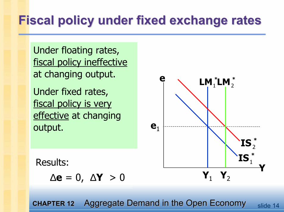
Under floating rates, a fiscal expansion would raise e. To keep e from rising, the central bank must sell domestic currency, which increases Mand shifts LM* right.

Under floating rates, fiscal policy ineffectiveat changing output.

Under fixed rates,fiscal policy is very effective at changing output.

Y

e

Y1

e1

1*LM

1*IS2*IS

Y2

2*LM

Results:

∆e = 0, ∆Y > 0


Mon. policy under fixed exchange ratesMon. policy under fixed exchange rates

2*LM

An increase in M would shift LM* right and reduce e.

Y

e

Y1

1*LM

1*IS

e1

To prevent the fall in e, the central bank must buy domestic currency, which reduces M and shifts LM* back left.

Results: ∆e = 0, ∆Y = 0

Under floating rates, monetary policy is very effective at changing output.

Under fixed rates,monetary policy cannot be used to affect output.

2*LM


Trade policy under fixed exchange ratesTrade policy under fixed exchange rates

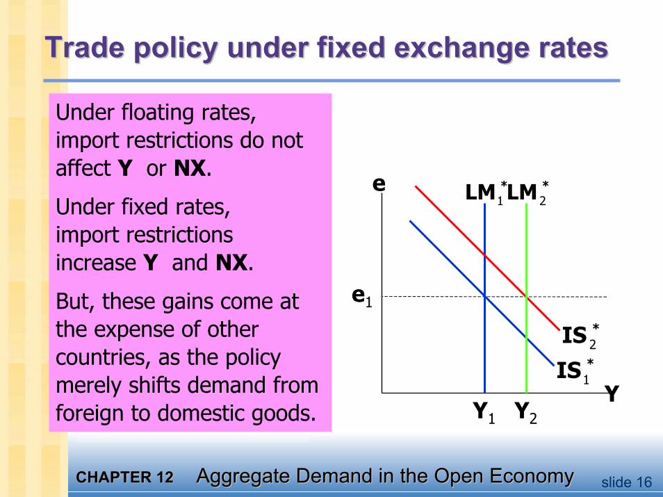
A restriction on imports puts upward pressure on e.

Results:

∆e = 0, ∆Y > 0

To keep e from rising, the central bank must sell domestic currency, which increases Mand shifts LM* right.

Under floating rates, import restrictions do not affect Y or NX.

Under fixed rates,import restrictions increase Y and NX.

But, these gains come at the expense of other countries, as the policy merely shifts demand from foreign to domestic goods.

Y

e

Y1

e1

1*LM

1*IS2*IS

Y2

2*LM


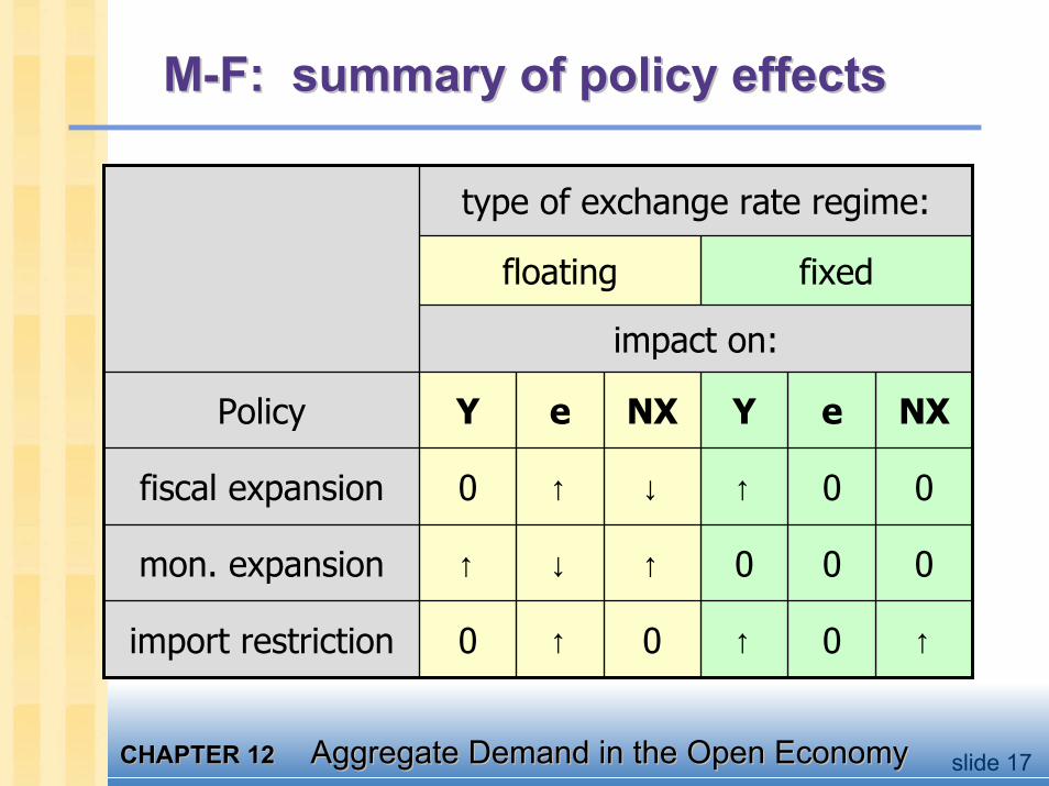
MM--F: summary of policy effectsF: summary of policy effects

↑0↑0↑0import restriction

000↑↓↑mon. expansion

00↑↓↑0fiscal expansion

NXeYNXeYPolicy

impact on:

fixedfloating

type of exchange rate regime:


InterestInterest--rate differentialsrate differentialsTwo reasons why r may differ from r*

country risk:The risk that the country’s borrowers will default on their loan repayments because of political or economic turmoil. Lenders require a higher interest rate to compensate them for this risk. expected exchange rate changes:If a country’s exchange rate is expected to fall, then its borrowers must pay a higher interest rate to compensate lenders for the expected currency depreciation.


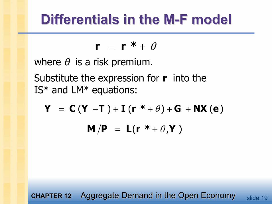
Differentials in the MDifferentials in the M--F modelF model

*r r θ= +where θ is a risk premium.

Substitute the expression for r into the IS* and LM* equations:

( ) ( ) ( )*Y C Y T I r G NX e= − + + + +θ

( , )*M P L r Y= + θ


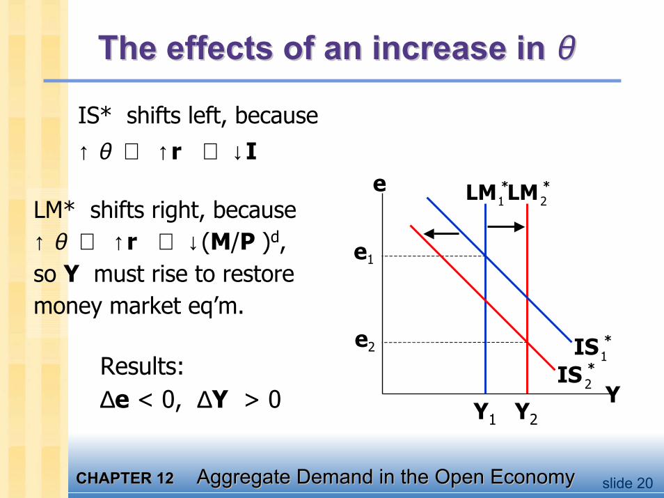
The effects of an increase in The effects of an increase in θθ

IS* shifts left, because ↑ θ ⇒ ↑ r ⇒ ↓ I

2*LM

Y

e

Y1

e1

1*LM

1*IS

2*IS

e2

Y2

LM* shifts right, because ↑ θ ⇒ ↑ r ⇒ ↓ (M/P )d,so Y must rise to restore money market eq’m.

Results: ∆e < 0, ∆Y > 0


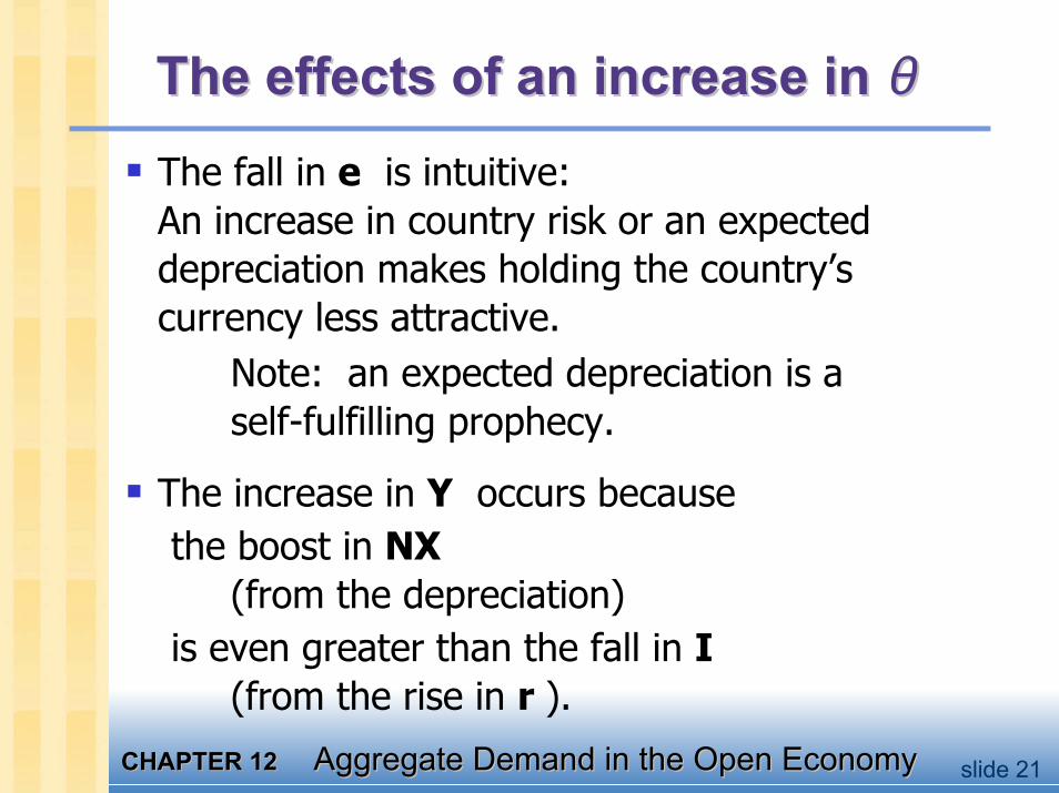
The effects of an increase in The effects of an increase in θθThe fall in e is intuitive: An increase in country risk or an expected depreciation makes holding the country’s currency less attractive.

Note: an expected depreciation is a self-fulfilling prophecy.

The increase in Y occurs because the boost in NX

(from the depreciation)is even greater than the fall in I

(from the rise in r ).


Why income might not riseWhy income might not rise

The central bank may try to prevent the depreciation by reducing the money supply

The depreciation might boost the price of imports enough to increase the price level (which would reduce the real money supply)

Consumers might respond to the increased risk by holding more money.

Each of the above would shift LM* leftward.


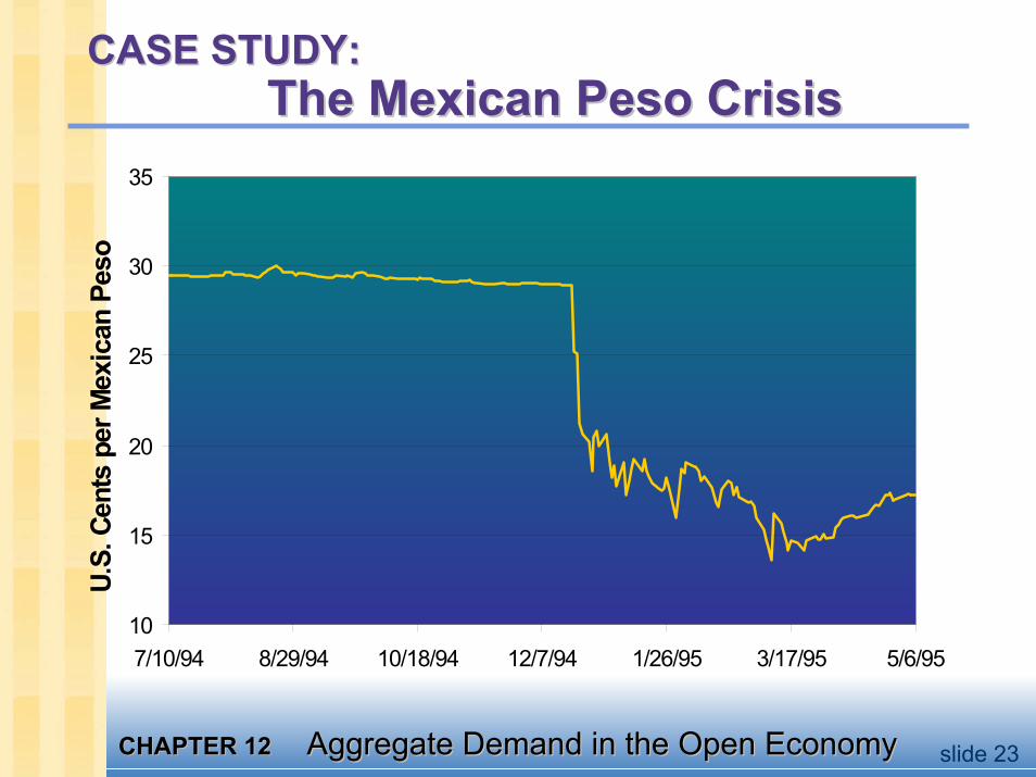
CASE STUDY: CASE STUDY: The Mexican Peso CrisisThe Mexican Peso Crisis

10

15

20

25

30

35

7/10/94 8/29/94 10/18/94 12/7/94 1/26/95 3/17/95 5/6/95

U.S.

Cen

ts p

er M

exic

an P

eso


The Peso Crisis didn’t just hurt MexicoThe Peso Crisis didn’t just hurt Mexico

U.S. goods more expensive to Mexicans– U.S. firms lost revenue– Hundreds of bankruptcies along

U.S.-Mex border

Mexican assets worth less in dollars– Affected retirement savings of

millions of U.S. citizens


Understanding the crisisUnderstanding the crisisIn the early 1990s, Mexico was an attractive place for foreign investment.

During 1994, political developments caused an increase in Mexico’s risk premium (θ ):• peasant uprising in Chiapas • assassination of leading presidential

candidateAnother factor: The Federal Reserve raised U.S. interest rates several times during 1994 to prevent U.S. inflation. (So, ∆r* > 0)


Understanding the crisisUnderstanding the crisisThese events put downward pressure on the peso.

Mexico’s central bank had repeatedly promised foreign investors that it would not allow the peso’s value to fall,so it bought pesos and sold dollars to “prop up” the peso exchange rate.

Doing this requires that Mexico’s central bank have adequate reserves of dollars. Did it?


Dollar reserves of Dollar reserves of Mexico’s central bankMexico’s central bank

December 1993 ……………… $28 billion

August 17, 1994 ……………… $17 billion

December 1, 1994 …………… $ 9 billion

December 15, 1994 ………… $ 7 billion

December 1993 ……………… $28 billion

August 17, 1994 ……………… $17 billion

December 1, 1994 …………… $ 9 billion

December 15, 1994 ………… $ 7 billion

During 1994, Mexico’s central bank hid the fact that its reserves were being depleted.


the disasterthe disasterDec. 20: Mexico devalues the peso by 13%

(fixes e at 25 cents instead of 29 cents)Investors are shocked shocked ! ! !…and realize the central bank must be running out of reserves…↑θ, Investors dump their Mexican assets and pull their capital out of Mexico.

Dec. 22: central bank’s reserves nearly gone. It abandons the fixed rate and lets e float.

In a week, e falls another 30%.


The rescue packageThe rescue package1995: U.S. & IMF set up $50b line of credit to provide loan guarantees to Mexico’s govt.

This helped restore confidence in Mexico, reduced the risk premium.

After a hard recession in 1995, Mexico began a strong recovery from the crisis.


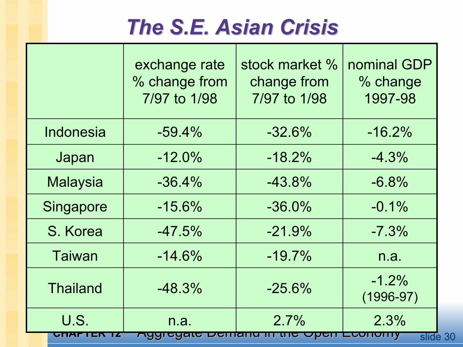
The S.E. Asian CrisisThe S.E. Asian Crisis

-1.2% (1996-97)-25.6%-48.3%Thailand

-6.8%-43.8%-36.4%Malaysia

-4.3%-18.2%-12.0%Japan

-0.1%-36.0%-15.6%Singapore

n.a.-19.7%-14.6%Taiwan

2.3%2.7%n.a.U.S.

-7.3%-21.9%-47.5%S. Korea

-16.2%-32.6%-59.4%Indonesia

nominal GDP % change 1997-98

stock market % change from 7/97 to 1/98

exchange rate % change from

7/97 to 1/98


Floating vs. Fixed Exchange RatesFloating vs. Fixed Exchange RatesArgument for floating rates:

allows monetary policy to be used to pursue other goals (stable growth, low inflation)

Arguments for fixed rates:

avoids uncertainty and volatility, making international transactions easier

disciplines monetary policy to prevent excessive money growth & hyperinflation


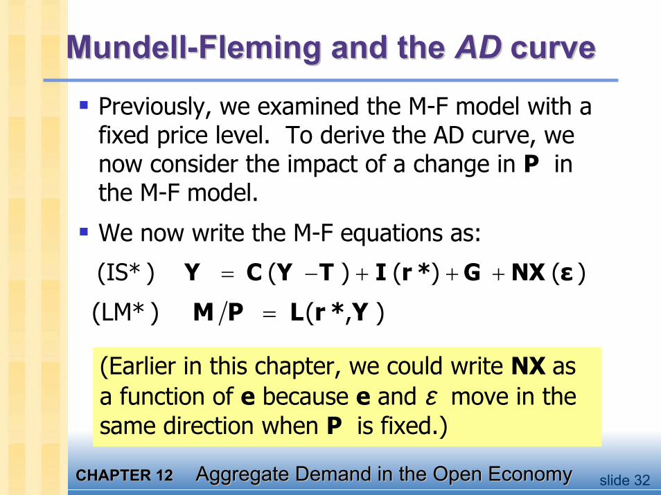
MundellMundell--Fleming and the Fleming and the ADAD curve curve Previously, we examined the M-F model with a fixed price level. To derive the AD curve, we now consider the impact of a change in P in the M-F model.

We now write the M-F equations as:

( ) ( ) ( ) ( )*Y C Y T I r G NX ε= − + + +IS*

( ) ( , )*M P L r Y=LM*

(Earlier in this chapter, we could write NX as a function of e because e and ε move in the same direction when P is fixed.)


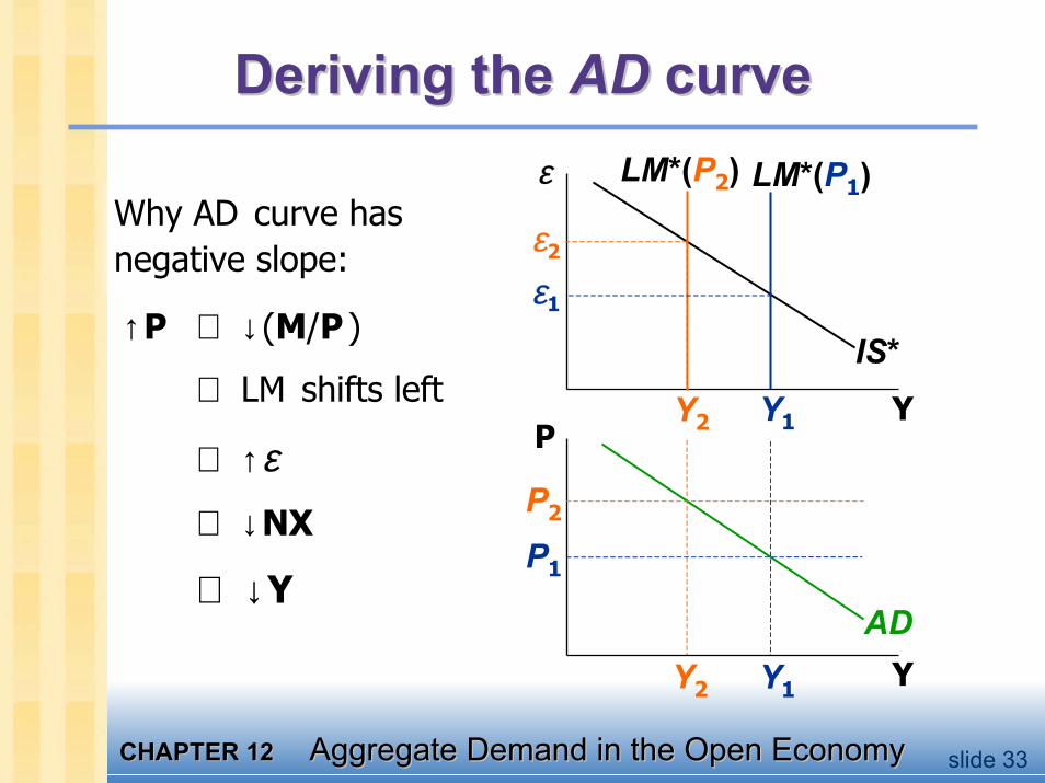
Deriving the Deriving the ADAD curvecurve

Y1Y2 Y

ε

Y

P

IS*

LM*(P1)LM*(P2)

AD

P1

P2

Y2 Y1

ε2

ε1

Why AD curve has negative slope:

↑P ⇒ ↓ (M/P )

⇒ LM shifts left

⇒ ↑ ε⇒ ↓ NX

⇒ ↓ Y


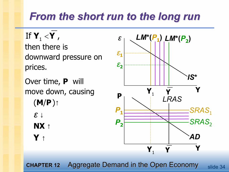
From the short run to the long runFrom the short run to the long run

then there is downward pressure on prices.

1If ,Y Y< LM*(P1)

ε1

ε2

P1 SRAS1

1Y

1Y Y

ε

Y

P

IS*

AD

Y

YLRAS

LM*(P2)

P2 SRAS2

Over time, P will move down, causing

(M/P )↑ε ↓NX ↑Y ↑


Large: between small and closedLarge: between small and closed

Many countries - including the U.S. - are neither closed nor small open economies.

A large open economy is in between the polar cases of closed & small open.

Consider a monetary expansion:• Like in a closed economy,

∆M > 0 ⇒ ↓ r ⇒ ↑ I (though not as much)• Like in a small open economy,

∆M > 0 ⇒ ↓ ε ⇒ ↑ NX (though not as much)


Chapter summaryChapter summary1. Mundell-Fleming model

the IS-LM model for a small open economy.takes P as givencan show how policies and shocks affect income and the exchange rate

2. Fiscal policyaffects income under fixed exchange rates, but not under floating exchange rates.


Chapter summaryChapter summary3. Monetary policy

affects income under floating exchange rates. Under fixed exchange rates, monetary policy is not available to affect output.

4. Interest rate differentialsexist if investors require a risk premium to hold a country’s assets.An increase in this risk premium raises domestic interest rates and causes the country’s exchange rate to depreciate.


Chapter summaryChapter summary5. Fixed vs. floating exchange rates

Under floating rates, monetary policy is available for can purposes other than maintaining exchange rate stability.Fixed exchange rates reduce some of the uncertainty in international transactions.


Documents

Mankiw 5/e Chapter 12: Agg Demand in the Open Economycameron.edu/~abduls/econ5213/Pdf/ch12.pdfCHAPTER 12 Aggregate Demand in the Open Economy slide 1 Learning objectives The Mundell-Fleming