Manipulation Planning on Constraint Manifolds

Dmitry Berenson† Siddhartha S. Srinivasa‡† Dave Ferguson‡† James J. Kuffner†

†The Robotics Institute, Carnegie Mellon University ‡Intel Research Pittsburgh5000 Forbes Ave., Pittsburgh, PA, 15213, USA Pittsburgh, PA, 15213, USA

[dberenso, kuffner]@cs.cmu.edu [siddhartha.srinivasa, dave.ferguson]@intel.com

Abstract— We present the Constrained Bi-directional Rapidly-Exploring Random Tree (CBiRRT) algorithm for planning pathsin configuration spaces with multiple constraints. This algo-rithm provides a general framework for handling a variety ofconstraints in manipulation planning including torque limits,constraints on the pose of an object held by a robot, andconstraints for following workspace surfaces. CBiRRT extendsthe Bi-directional RRT (BiRRT) algorithm by using projectiontechniques to explore the configuration space manifolds thatcorrespond to constraints and to find bridges between them.Consequently, CBiRRT can solve many problems that the BiRRTcannot, and only requires one additional parameter: the allowableerror for meeting a constraint. We demonstrate the CBiRRT ona 7DOF WAM arm with a 4DOF Barrett hand on a mobile base.The planner allows this robot to perform household tasks, solvepuzzles, and lift heavy objects.

I. INTRODUCTION

Our everyday lives are full of tasks that constrain ourmovement. Carrying a coffee mug, lifting a heavy object, orsliding a milk jug out of a refrigerator, are examples of tasksthat involve constraints imposed on our bodies as well as themanipulated objects. Enabling autonomous robots to performsuch tasks involves computing motions that are subject tomultiple, often simultaneous, task constraints.

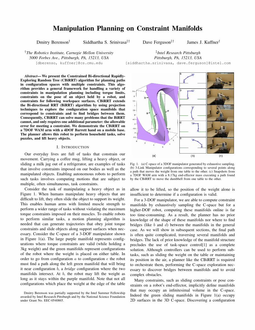
Consider the task of manipulating a heavy object as inFigure 1. When humans manipulate heavy objects that aredifficult to lift, they often slide the object to support its weight.This enables human arms with limited muscle strength toperform a wider range of tasks without violating the maximumtorque constraints imposed on their muscles. To enable robotsto perform similar tasks, a motion planning algorithm isneeded that can generate trajectories that obey joint torqueconstraints and slide objects along support surfaces when nec-essary. Consider the C-space of a 3-DOF manipulator shownin Figure 1(a). The large purple manifold represents config-urations where torque constraints are valid (while holding a3kg weight) and the green manifolds represent configurationsof the robot where the weight is placed on either table. Inorder to go from configuration a to configuration e the robotmust find a path along the left green manifold that will bringit near configuration b, a bridge configuration where the twomanifolds intersect. At b, the robot may lift the weight aslong as it stays within the purple manifold. Note that not allconfigurations which place the weight at the edge of the table

Dmitry Berenson was partially supported by the Intel Summer Fellowshipawarded by Intel Research Pittsburgh and by the National Science Foundationunder Grant No. EEC-0540865.

Fig. 1. (a) C-space of a 3DOF manipulator generated by exhaustive sampling.(b) 3-Link Manipulator configurations corresponding to several points alonga path that moves the weight from one table to the other. (c) Snapshots froma 7DOF WAM arm with a 8.17kg end-effector mass executing a path foundby the CBiRRT to move the dumbbell from one table to the other.

allow it to be lifted, so the position of the weight alone isinsufficient to determine if a configuration is valid.

For a 3-DOF manipulator, we are able to compute constraintmanifolds by exhaustively sampling the C-space but for ahigher-DOF robot, computing these manifolds online is fartoo time-consuming. As a result, the planner has no priorknowledge of the shape of these manifolds nor where to findbridges (like b and d) between the manifolds in the generalcase. As we will show in subsequent sections, the final pathis often quite complicated, traversing several manifolds andbridges. The lack of prior knowledge of the manifold structureprecludes the use of task-space control[1] as a completesolution. Although controllers can be used to perform sub-tasks, such as sliding the weight on the table or maintainingits position in the air, a planner like the CBiRRT is requiredto orchestrate them, performing the C-space exploration nec-essary to discover bridges between manifolds and to avoidcomplex obstacles.

Many constraints, such as sliding constraints or pose con-straints on a robot’s end-effector, implicitly define manifoldsthat may occupy an infinitesimal volume in the C-space.Indeed the green sliding manifolds in Figure 1(a) occupy2D surfaces in the 3D C-space. Discovering a configuration

that lies on such a manifold through randomly samplingjoint-values is extremely unlikely. This fact precludes theuse of standard sampling-based planners such as RRTs orProbabilistic Road Maps (PRMs) that sample C-space directly.

This paper introduces the Constrained Bi-directionalRapidly-Exploring Random Tree (CBiRRT) planner, whichaddresses the problem of sampling on constraint manifolds.CBiRRT first samples in the C-space and then uses projectionoperations to move samples onto constraint manifolds whennecessary. This technique allows the planner to explore con-straint manifolds efficiently and to construct paths embeddedin them. CBiRRT also exploits the “connect” sampling heuris-tic of the RRT to find bridges between manifolds correspond-ing to different constraints, such as sliding an object and thenlifting it. Such a slide-and-lift motion can be found using asingle extension operation of the CBiRRT algorithm.

In the rest of the paper, we first give a brief overviewof previous work relevant to constrained motion planning.We then introduce the CBiRRT algorithm and describe howto formulate various types of constraints. We then presentseveral example problems and experiments which illustrate theability of the CBiRRT to plan for tasks that were previouslyunachievable without special-purpose planners. The paper endswith a discussion of the advantages and limitations of ourapproach.

II. BACKGROUND

The CBiRRT algorithm builds on several developments inmotion planning and control research in robotics. In motionplanning, a number of efficient sampling-based planning al-gorithms have been developed recently for searching high-dimensional C-spaces. Although CBiRRT is based on theRapidly-exploring Random Tree (RRT) algorithm by LaValleand Kuffner[2], it is possible to adapt some of the ideasand techniques in this paper to other search algorithms. Weselected RRTs for their ability to explore C-space whileretaining an element of “greediness” in their search for asolution. The greedy element is most evident in the bidi-rectional version of the RRT algorithm (BiRRT), where twotrees, one grown from the start configuration and one grownfrom the goal configuration, take turns exploring the spaceand attempting to connect to each other. In this paper, wedemonstrate that such a search strategy is also effective formotion planning problems involving constraints when it iscoupled with projection methods that move C-space samplesonto constraint manifolds. Note that RRTs have also beenpreviously extended to planning for hybrid control systems[3],which is similar to planning with constraint manifolds.

In the robotics literature, projection methods have arisenin the context of research in controls and inverse kinematics.Iterative inverse kinematics algorithms use projection methodsbased on the pseudo-inverse or transpose of the Jacobian toiteratively move a robot’s end-effector closer to some de-sired workspace transformation (e.g. [4]). Sentis and Khatib’spotential-field approach[1] uses recursive null-space projec-tion to project a robot’s configuration away from obstacles and

Algorithm 1: CBiRRT(Qs, Qg)

Ta.Init(Qs); Tb.Init(Qg);1

while TimeRemaining() do2

qrand ← RandomConfig();3

qanear ← NearestNeighbor(Ta, qrand);4

qareached ← ConstrainedExtend(Ta, qanear, qrand);5

qbnear ← NearestNeighbor(Tb, qareached);6

qbreached ← ConstrainedExtend(Tb, qbnear, qareached);7

if qareached = qbreached then8

P ← ExtractPath(Ta, qareached, Tb, qbreached);9

return SmoothPath(P );10

else11

Swap(Ta, Tb);12

end13

end14

return NULL;15

toward desirable configurations. The Randomized GradientDescent (RGD)[5] method uses random-sampling of the C-space to iteratively project a sample towards an arbitraryconstraint[6]. Though [5] showed how to incorporate RGDinto a randomized planner, it requires significant parameter-tuning and they dealt only with closed-chain kinematic con-straints, which are a special case of the pose constraints usedin this paper. Furthermore, Stilman [7] showed that whenRGD is extended to work with more general pose constraintsit is significantly less efficient than Jacobian pseudo-inverseprojection and it is sometimes unable to meet more stringentconstraints. Inspired by this result, we also use the Jacobianpseudo-inverse projection method, though our framework canuse any projection method that moves samples on to constraintmanifolds efficiently.

In some previous work the problem of planning for anobject’s motion is subdivided into planning a path in alower-dimensional space[8][9] that lies within some manifold(like the surface of a table) or using a pre-scripted lower-dimensional path[10][11][12]. The lower-dimensional path isthen followed in the full C-space of the robot. This approachsuffers from feasibility problems because a lower-dimensionalpath may not be trackable by the robot because of joint limitsor collisions. The CBiRRT algorithm therefore plans in thefull C-space of the robot, which incurs a larger computationalburden but allows it to handle more general types of constraintsand to find paths through multiple constraint manifolds.

III. THE CBIRRT ALGORITHM

The CBiRRT algorithm (see Algorithm 1) operates bygrowing two trees in the C-space of the robot. During eachiteration of the algorithm one of the trees grows a branchtoward a randomly-sampled configuration qrand using theConstrainedExtend function. The branch grows as far aspossible toward qrand but may be stalled due to collision orconstraint violation and will terminate at qareached. The othertree then grows a branch toward qareached, again growing as far

Algorithm 2: ConstrainedExtend(T , qnear, qtarget)

qs ← qnear; qolds ← qnear;1

while true do2

if qtarget = qs then3

return qs;4

else if |qtarget − qs| >∣∣qolds − qtarget∣∣ then5

return qolds ;6

end7

qs ← qs + min(∆qstep, |qtarget − qs|) (qtarget−qs)|qtarget−qs| ;8

qs ← ConstrainConfig(qolds , qs);9

if qs 6= NULL and CollisionFree(qolds , qs) then10

T .AddVertex(qs);11

T .AddEdge(qolds , qs);12

qolds ← qs;13

else14

return qolds ;15

end16

end17

Algorithm 3: SmoothPath(P )

while TimeRemaining() do1

Tshortcut ← {};2

i ← RandomInt(1, P.size− 1);3

j ← RandomInt(i, P.size);4

qreached ← ConstrainedExtend(Tshortcut, Pi, Pj);5

if qreached = Pj and6

Length(Tshortcut) < Length(Pi · · ·Pj) thenP ← [P1 · · ·Pi, Tshortcut, Pj+1 · · ·P.size];7

end8

end9

return P ;10

as possible toward this configuration. If the other tree reachesqareached, the trees have connected and a path has been found.If not, the trees are swapped and the above process is repeated.

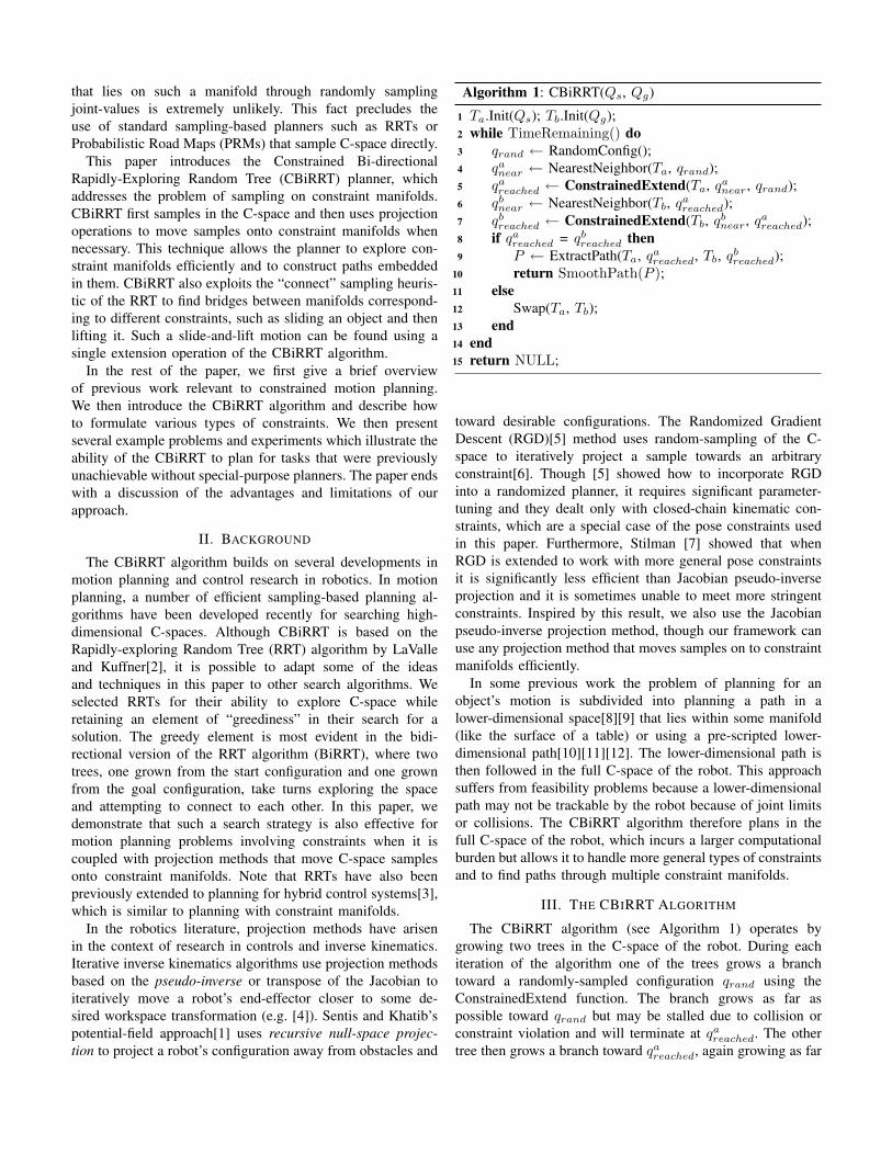
The ConstrainedExtend function (see Algorithm 2) worksby iteratively moving from a configuration qnear toward aconfiguration qtarget with a step size of ∆qstep. After each steptoward qtarget, the function checks if the new configurationqs has reached qtarget or if it is not making progress towardqtarget, in either case the function terminates. If the aboveconditions are not true then the algorithm takes a step towardqtarget and passes the new qs to the ConstrainConfig function.The ConstrainConfig function is problem-specific, and severalexamples of such functions are given in the example problems.If ConstrainConfig is able to project qs to a constraint manifoldand this qs is not in collision, the new qs is added tothe tree and the above process is repeated. Otherwise, Con-strainedExtend terminates (see Figure 2). ConstrainedExtendalways returns the last configuration reached by the extensionoperation.

The CollisionFree(qolds , qs) function checks collision by

Fig. 2. Depiction of one extend operation that moves across two manifolds. Theoperation starts at qnear , which is a node of a search tree on constraint manifold C1and iteratively moves toward qtarget, which is a randomly-sampled configuration inC-space. Each step toward qtarget is constrained using the ConstrainConfig function tolie on the closest constraint manifold.

stepping along the interval between qolds and qs. Collision-checking can also be treated as a constraint, and can beincorporated in to the ConstrainConfig function.

The SmoothPath function uses the “short-cut” smoothingmethod to iteratively shorten the path from the start to thegoal[13]. Since we use the ConstrainedExtend function foreach short-cut, we are guaranteed that the constraints willbe met along the smoothed path. Also, it is important tonote that a short-cut generated by ConstrainedExtend betweentwo nodes is not necessarily the shortest path between thembecause the nodes may have been projected in an arbitraryway. This necessitates checking whether Length(Pshortcut) isshorter than the original path between i and j.

Besides handling constraints, an important difference be-tween CBiRRT and the standard BiRRT algorithm is thatmultiple start and goal configurations (Qs and Qg , respec-tively) can be used to initialize the trees. This capabilityis important because many of the constraints that we dealwith can invalidate paths between distant configurations. Forinstance, moving from an elbow-up configuration to an elbow-down configuration may not be possible if the end-effector isconstrained to not move in a certain direction. Thus, when werun CBiRRT, we usually seed it with multiple IK solutions forboth the start and goal configuration of an object we are tryingto manipulate. Implementing this multiple start/goal capabilityis also straightforward. If a tree is stored as an array of nodeswith each node containing a pointer to its parent, we define aplaceholder node as the start/goal and set it as the parent ofthe Qs/Qg nodes. The algorithm then proceeds as normal.

Another key point is that the BiRRT algorithm is a specialcase of the CBiRRT algorithm. If the ConstrainConfig() func-tion always returns true without modifying qs (i.e. there areno constraints) and |Qs| = |Qg| = 1, the CBiRRT and BiRRTalgorithms behave identically.

IV. CONSTRAINTS

Our planner is capable of handling tasks with multipleconstraints as long as each constraint can be evaluated asa function of the robot’s configuration. The algorithm canhandle arbitrary strategies for dealing with these constraints byencoding these strategies in the ConstrainConfig function. Inthis paper, we focus on two general strategies for dealing withconstraints: rejection and projection. Neither strategy requiresan analytical representation of the constraint manifold.

In the rejection strategy, we simply check if a given configu-ration of the robot meets a certain constraint, if it does not, wedeem the configuration invalid. This strategy is effective whenthere is a high probability of randomly sampling configurationsthat satisfy this constraint, in other words, the constraintmanifold occupies some significant volume in the C-space.

The projection strategy is robust to more stringent con-straints, namely ones whose manifolds do not occupy asignificant volume of the C-space. However, this robustnesscomes at the price of requiring a distance function to evaluatehow close a given configuration is to the constraint manifold.The projection strategy works by using gradient descent toiteratively reduce the distance to the constraint manifold andterminates when a configuration is found that is within somethreshold ε of the manifold.

A. Object/End-Effector Pose Constraints

Many of the constraints we deal with are restrictions onthe pose of an object being manipulated by a robot arm orthe arm’s end-effector, which were first discussed in [14].We assume that the arm has grasped the object it is holdingrigidly, effectively translating constraints on the object intoconstraints on the end-effector. Thus we will treat constraintson the object and constraints on the robot’s end-effector asconceptually equivalent.

Throughout this paper, we will be using transformationmatrices of the form Tab , which specifies the pose of b inthe coordinates of frame a. Tab , written in homogeneouscoordinates, consists of a 3×3 rotation matrix Rab and a 3×1translation vector tab .

Tab =[

Rab tab0 1

](1)

The first step to working with constraints on the object’spose is to define a reference transform for the object T0

obj aswell as a reference transform for the constraint T0

c . T0c can be

stationary in the world (for instance the hinge of a door) or canchange depending on the pose of the object. Constraints arethen defined in terms of the permissible differences betweenT0obj and T0

c as in Equation 2.

C =

cxmin cxmax

cymin cymax

czminczmax

cψmincψmax

cθmincθmax

cφmin cφmax

(2)

The first three rows of C bound the allowable translationalong the x, y, and z axes and the last three bound the allowablerotations about those axes, all in the T0

c frame. Note that thisassumes the Roll-Pitch-Yaw (RPY) Euler Angle convention.

Such a representation has several advantages. First, speci-fying constraints is intuitive as will be shown in the exampleproblems. Second, this representation allows us to define adistance function for pose constraints that is very fast tocompute. Given a configuration qs, we define the Displace-mentFromConstraint(C, T0

c , qs) function as follows:First compute the forward kinematics at qs to get T0

obj . Thencompute the pose of the object in constraint-frame coordinates.

Tcobj = (T0c)−1T0

obj (3)

Then convert Tcobj from a transformation matrix to a 6-dimensional displacement vector dc, consisting of displace-ments in x, y, z, roll, pitch and yaw:

dc =

tcobj

arctan2(Rcobj32 ,Rcobj33)

−arcsin(Rcobj31)arctan2(Rcobj21 ,R

cobj11)

(4)

Taking into account the bounds in C, we get the displace-ment to this constraint ∆x:

∆xi =

dci − Cimaxif dci > Cimax

dci − Cimin if dci < Cimin

0 otherwise(5)

where i indexes through the six rows of C and six elementsof ∆x and dc. The distance to the constraint is then ‖∆x‖.Note that this distance function is only used when projectingto pose constraints, the standard Euclidean distance functionis used when selecting nearest-neighbors in the RRT.

B. Using Projection with Pose Constraints

In order to meet pose constraints, we employ a gradient-descent projection method based on the Jacobian-pseudo in-verse which is similar to that used in [7] (see Algorithm 4),however any effective projection method is acceptable.

Algorithm 4: ProjectConfig(qolds , qs, C, T0c)

while true do1

∆x ← DisplacementFromConstraint(C, T0c , qs);2

if ‖∆x‖ < ε then return qs;3

J ← GetJacobian(qs);4

∆qerror ← JT (JJT )−1∆x;5

qs ← (qs −∆qerror);6

if∣∣qs − qolds ∣∣ > 2∆qstep or OutsideJointLimit(qs)7

then return NULL;end8

The GetJacobian function returns the Jacobian of the ma-nipulator with the rotational part of the Jacobian in the RPYconvention. Converting the standard angular-velocity Jacobian

to the RPY Jacobian is done by applying the linear transfor-mation Erpy(q), which is defined in the Appendix of [7].

C. Torque Constraints

Another constraint we will deal with is the constrainton joint torques when lifting heavy objects. Since we willbe employing the rejection strategy with respect to torqueconstraints, we need only calculate the torques on the jointsin a given qs. This is done using standard Recursive Newton-Euler techniques described in [15]. To incorporate the objectinto the robot model, we take a weighted average of the centersof mass of the end-effector and the object and set that as themass and center of mass of the end-effector. We will refer tothe combined mass as m. Note that this formulation only takesinto account the torque necessary to maintain a given qs, i.e.it assumes the robot’s motion is quasi-static.

So far this section has described how to find displacementsto a given constraint and how to handle torque constraints.However when there are multiple constraints, the planner mustmake decisions about which constraints to project to andmust sometimes use a combination of rejection and projectionstrategies to plan a path. In the following three sections, wedescribe three example problems which deal with variousconstraints and show effective methods for planning pathsfor these problems based on the above two strategies.We alsodescribe implementation details and simulation results for aninstance of each type of problem.

V. EXAMPLE A: THE MAZE PUZZLE

In this problem, the robot arm must solve a maze puzzle bydrawing a path through the maze with a pen (see Figure 3(a)).The constraint is that the pen must always be touching the tablehowever the pen is allowed to pivot about the contact point upto an angle of α. We define T0

obj to be at the tip of the pen withno rotation relative to the world frame. We define T0

c to be atthe height of the table at the center of the maze with no rotationrelative to the world frame (z being up). This example is meantto demonstrate that CBiRRT is capable of solving multiplenarrow passage problems while still moving on a constraintmanifold. It is also meant to demonstrate the generality of theCBiRRT; no special-purpose planner is needed even for sucha specialized task. The ConstrainConfig function used for thisexample is shown in Algorithm 5.

A. Implementation and Results

The robot’s base is fixed in this problem. IK solutions weregenerated for both the start and goal position of the pen usingthe given grasp and input as Qs and Qg . For this examplewe place the base roughly halfway between the start and goalpositions of the object such that it does not collide with anyobstacles. We then compute all IK solutions for both the startand goal positions of the object up to a 0.05rad discretizationof the arm’s first joint angle. The values in Table I representthe average of 10 runs for different α values. Runtimes witha “>” denote that there was at least one run that did not

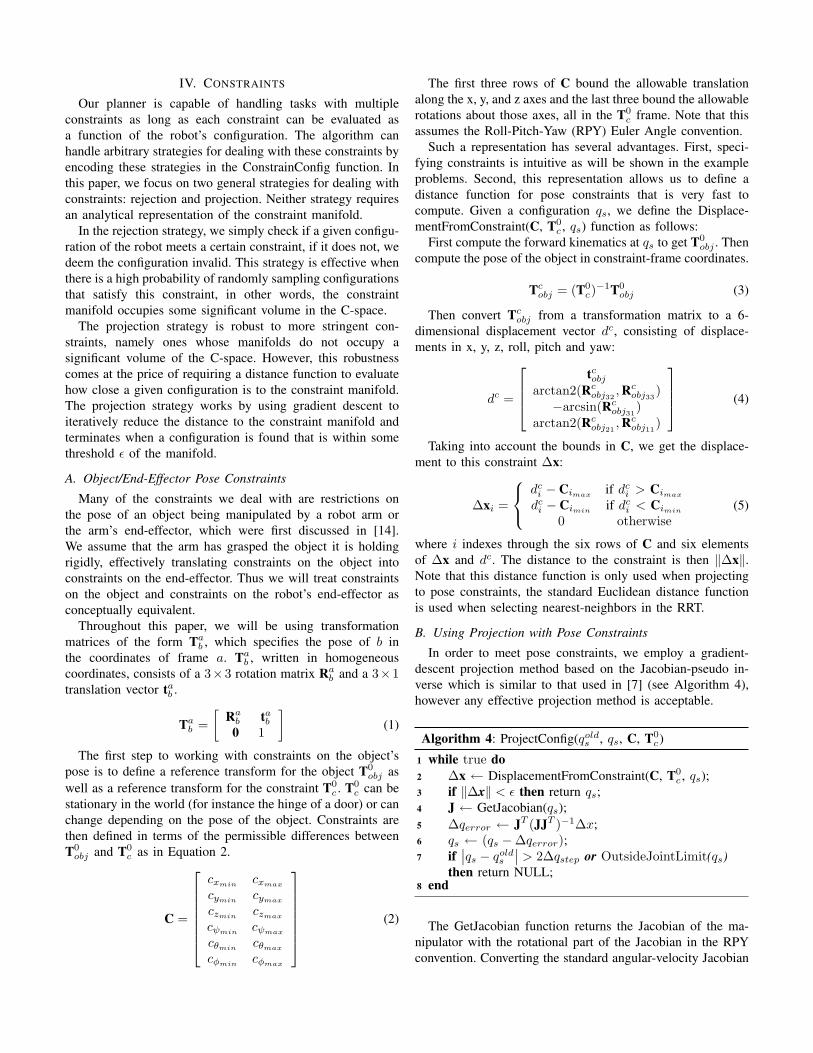
Fig. 3. Example problems. (a) Maze Puzzle (b) Heavy object with sliding surfaces (c)Heavy object with sliding surfaces and pose constraints. Yellow planes represent surfacesthat can be used for sliding.

α(rad.) 0.0 0.1 0.2 0.3 0.4 0.5

Avg. Runtime(s) >83.5 >58.8 >49.0 19.5 14.3 15.2Success Rate 40% 60% 90% 100% 100% 100%

TABLE I: SIMULATION RESULTS FOR EXAMPLE A

terminate before 120 seconds. For such runs, 120 was used incomputing the average. ∆qstep = 0.05 and ε = 0.001.

The shorter runtimes and high success rates for larger αvalues demonstrate that the more freedom we allow for thetask, the easier it is for the algorithm to solve it. This showsa key advantage of formulating the constraints as bounds onallowable pose as opposed to requiring the pose of the objectto conform exactly to a specified value. For problems wherewe do not need to maintain an exact pose for an object wecan allow more freedom, which makes the problem easier. SeeFigure 4 for an example trajectory of the tip of the pen.

VI. EXAMPLE B: HEAVY OBJECT WITH SLIDINGSURFACES

In this problem the task is to move a heavy object (adumbbell in this example) from a start position to a given goalposition (see Figure 3(b)). It is not known a-priori whether theobject is light enough to lift directly from its start position or ifit can be placed directly into its goal position without sliding.Sliding surfaces are also provided so that the planner mayuse these if necessary. Each sliding surface is a rectangle of

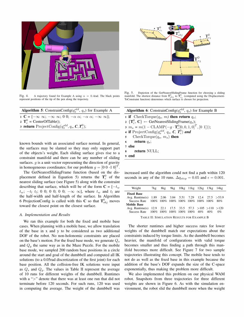
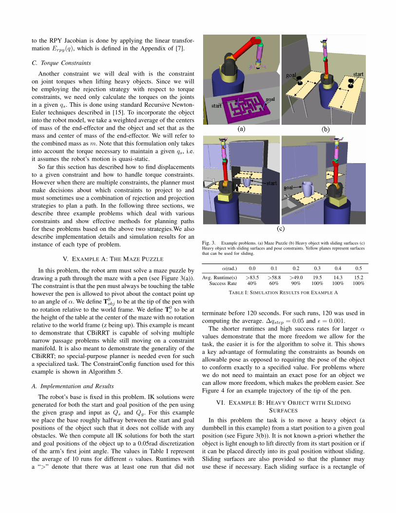
Fig. 4. A trajectory found for Example A using α = 0.4rad. The black pointsrepresent positions of the tip of the pen along the trajectory.

Algorithm 5: ConstrainConfig(qolds , qs) for Example A

C = [−∞ ∞; −∞ ∞; 0 0; −α α; −α α; −∞ ∞];1

T0c = CenterOfTable();2

return ProjectConfig(qolds , qs,C,T0c);3

known bounds with an associated surface normal. In general,the surfaces may be slanted so they may only support partof the objects’s weight. Each sliding surface gives rise to aconstraint manifold and there can be any number of slidingsurfaces. g is a unit vector representing the direction of gravityin homogeneous coordinates; for our problem g = [0 0 -1 0]T .

The GetNearestSlidingFrame function (based on the dis-placement defined in Equation 5) returns the T0

c of thenearest sliding surface (see Figure 5) along with the constraintdescribing that surface, which will be of the form C = [−twtw; −tl tl; 0 0; 0 0; 0 0; −∞ ∞], where tw and tl arethe half-width and half-length of the surface. In Algorithm6 ProjectionConfig is called with this C so that T0

obj movestoward the closest point on the closest surface.

A. Implementation and Results

We ran this example for both the fixed and mobile basecases. When planning with a mobile base, we allow translationof the base in x and y to be considered as two additionalDOF of the robot. No non-holonomic constraints are placedon the base’s motion. For the fixed base mode, we generate Qsand Qg the same way as in the Maze Puzzle. For the mobilebase mode, we sampled 200 random base positions in a circlearound the start and goal of the dumbbell and computed all IKsolutions (to a 0.05rad discretization of the first joint) for eachbase position. All the collision-free IK solutions were inputas Qs and Qg . The values in Table II represent the averageof 10 runs for different weights of the dumbbell. Runtimeswith a “>” denote that there was at least one run that did notterminate before 120 seconds. For such runs, 120 was usedin computing the average. The weight of the dumbbell was

Fig. 5. Depiction of the GetNearestSlidingFrame function for choosing a slidingmanifold. The shortest distance from T0

obj to T0ci

(computed using the Displacement-ToConstraint function) determines which surface is chosen for projection.

Algorithm 6: ConstrainConfig(qolds , qs) for Example B

if CheckTorque(qs, m) then return qs;1

{T0c , C} ← GetNearestSlidingFrame(qs);2

ms = m(1− CLAMP(−g · T0c [0, 0, 1, 0]T , [0 1]));3

if ProjectConfig(qolds , qs, C, T0c) and4

CheckTorque(qs, ms) then5

return qs;6

else7

return NULL;8

end9

increased until the algorithm could not find a path within 120seconds in any of the 10 runs. ∆qstep = 0.05 and ε = 0.001.

Weight 7kg 8kg 9kg 10kg 11kg 12kg 13kg 14kg

Fixed BaseAvg. Runtime(s) 1.89 2.06 3.84 5.51 7.29 12.4 27.5 >53.9

Success Rate 100% 100% 100% 100% 100% 100% 100% 80%Mobile BaseAvg. Runtime(s) 12.9 22.1 17.5 33.5 57.3 >105 >110 >120

Success Rate 100% 100% 100% 100% 100% 40% 40% 0%

TABLE II: SIMULATION RESULTS FOR EXAMPLE B

The shorter runtimes and higher success rates for lowerweights of the dumbbell match our expectations about theconstraints induced by torque limits. As the dumbbell becomesheavier, the manifold of configurations with valid torquebecomes smaller and thus finding a path through this man-ifold becomes more difficult. See Figure 7 for two sampletrajectories illustrating this concept. The mobile base tends tonot do as well as the fixed base in this example because theaddition of the base’s DOF expands the size of the C-spaceexponentially, thus making the problem more difficult.

We also implemented this problem on our physical WAMrobot. Snapshots from three trajectories for three differentweights are shown in Figure 6. As with the simulation en-vironment, the robot slid the dumbbell more when the weight

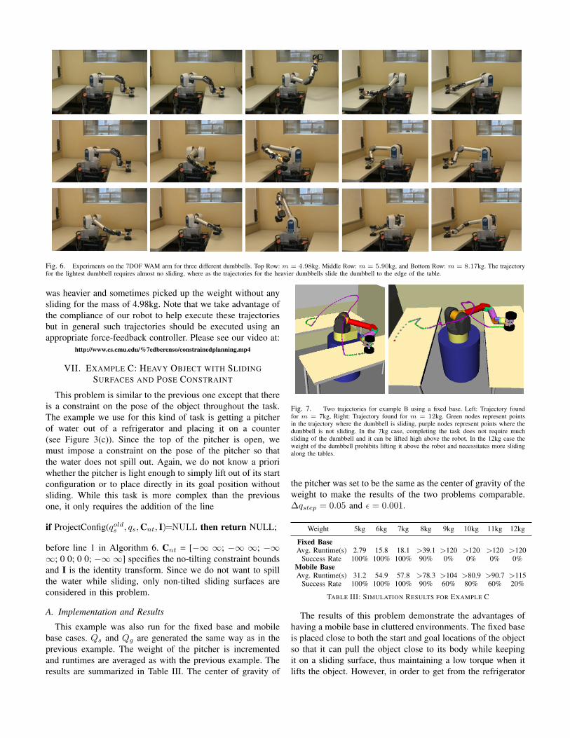
Fig. 6. Experiments on the 7DOF WAM arm for three different dumbbells. Top Row: m = 4.98kg. Middle Row: m = 5.90kg, and Bottom Row: m = 8.17kg. The trajectoryfor the lightest dumbbell requires almost no sliding, where as the trajectories for the heavier dumbbells slide the dumbbell to the edge of the table.

was heavier and sometimes picked up the weight without anysliding for the mass of 4.98kg. Note that we take advantage ofthe compliance of our robot to help execute these trajectoriesbut in general such trajectories should be executed using anappropriate force-feedback controller. Please see our video at:

http://www.cs.cmu.edu/%7edberenso/constrainedplanning.mp4

VII. EXAMPLE C: HEAVY OBJECT WITH SLIDINGSURFACES AND POSE CONSTRAINT

This problem is similar to the previous one except that thereis a constraint on the pose of the object throughout the task.The example we use for this kind of task is getting a pitcherof water out of a refrigerator and placing it on a counter(see Figure 3(c)). Since the top of the pitcher is open, wemust impose a constraint on the pose of the pitcher so thatthe water does not spill out. Again, we do not know a prioriwhether the pitcher is light enough to simply lift out of its startconfiguration or to place directly in its goal position withoutsliding. While this task is more complex than the previousone, it only requires the addition of the line

if ProjectConfig(qolds , qs,Cnt, I)=NULL then return NULL;

before line 1 in Algorithm 6. Cnt = [−∞ ∞; −∞ ∞; −∞∞; 0 0; 0 0; −∞∞] specifies the no-tilting constraint boundsand I is the identity transform. Since we do not want to spillthe water while sliding, only non-tilted sliding surfaces areconsidered in this problem.

A. Implementation and Results

This example was also run for the fixed base and mobilebase cases. Qs and Qg are generated the same way as in theprevious example. The weight of the pitcher is incrementedand runtimes are averaged as with the previous example. Theresults are summarized in Table III. The center of gravity of

Fig. 7. Two trajectories for example B using a fixed base. Left: Trajectory foundfor m = 7kg, Right: Trajectory found for m = 12kg. Green nodes represent pointsin the trajectory where the dumbbell is sliding, purple nodes represent points where thedumbbell is not sliding. In the 7kg case, completing the task does not require muchsliding of the dumbbell and it can be lifted high above the robot. In the 12kg case theweight of the dumbbell prohibits lifting it above the robot and necessitates more slidingalong the tables.

the pitcher was set to be the same as the center of gravity of theweight to make the results of the two problems comparable.∆qstep = 0.05 and ε = 0.001.

Weight 5kg 6kg 7kg 8kg 9kg 10kg 11kg 12kg

Fixed BaseAvg. Runtime(s) 2.79 15.8 18.1 >39.1 >120 >120 >120 >120

Success Rate 100% 100% 100% 90% 0% 0% 0% 0%Mobile BaseAvg. Runtime(s) 31.2 54.9 57.8 >78.3 >104 >80.9 >90.7 >115

Success Rate 100% 100% 100% 90% 60% 80% 60% 20%

TABLE III: SIMULATION RESULTS FOR EXAMPLE C

The results of this problem demonstrate the advantages ofhaving a mobile base in cluttered environments. The fixed baseis placed close to both the start and goal locations of the objectso that it can pull the object close to its body while keepingit on a sliding surface, thus maintaining a low torque when itlifts the object. However, in order to get from the refrigerator

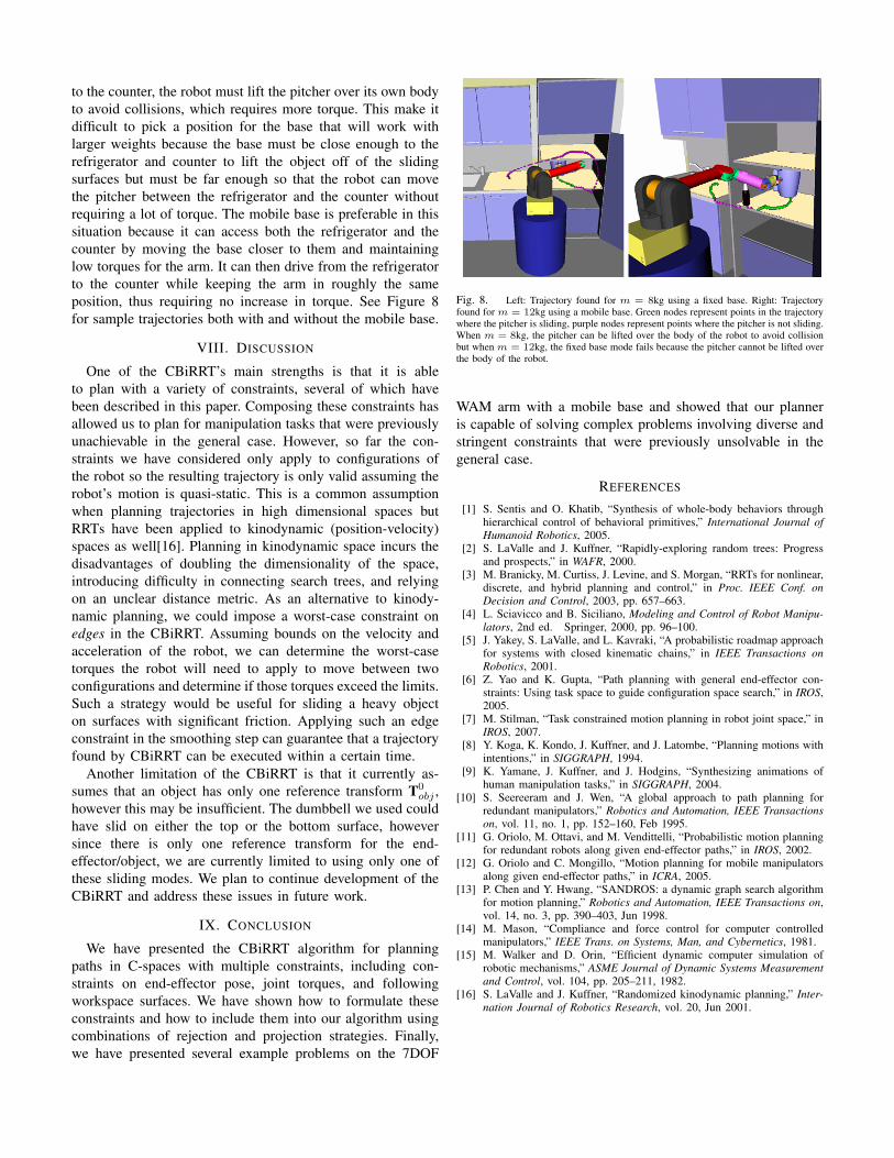
to the counter, the robot must lift the pitcher over its own bodyto avoid collisions, which requires more torque. This make itdifficult to pick a position for the base that will work withlarger weights because the base must be close enough to therefrigerator and counter to lift the object off of the slidingsurfaces but must be far enough so that the robot can movethe pitcher between the refrigerator and the counter withoutrequiring a lot of torque. The mobile base is preferable in thissituation because it can access both the refrigerator and thecounter by moving the base closer to them and maintaininglow torques for the arm. It can then drive from the refrigeratorto the counter while keeping the arm in roughly the sameposition, thus requiring no increase in torque. See Figure 8for sample trajectories both with and without the mobile base.

VIII. DISCUSSION

One of the CBiRRT’s main strengths is that it is ableto plan with a variety of constraints, several of which havebeen described in this paper. Composing these constraints hasallowed us to plan for manipulation tasks that were previouslyunachievable in the general case. However, so far the con-straints we have considered only apply to configurations ofthe robot so the resulting trajectory is only valid assuming therobot’s motion is quasi-static. This is a common assumptionwhen planning trajectories in high dimensional spaces butRRTs have been applied to kinodynamic (position-velocity)spaces as well[16]. Planning in kinodynamic space incurs thedisadvantages of doubling the dimensionality of the space,introducing difficulty in connecting search trees, and relyingon an unclear distance metric. As an alternative to kinody-namic planning, we could impose a worst-case constraint onedges in the CBiRRT. Assuming bounds on the velocity andacceleration of the robot, we can determine the worst-casetorques the robot will need to apply to move between twoconfigurations and determine if those torques exceed the limits.Such a strategy would be useful for sliding a heavy objecton surfaces with significant friction. Applying such an edgeconstraint in the smoothing step can guarantee that a trajectoryfound by CBiRRT can be executed within a certain time.

Another limitation of the CBiRRT is that it currently as-sumes that an object has only one reference transform T0

obj ,however this may be insufficient. The dumbbell we used couldhave slid on either the top or the bottom surface, howeversince there is only one reference transform for the end-effector/object, we are currently limited to using only one ofthese sliding modes. We plan to continue development of theCBiRRT and address these issues in future work.

IX. CONCLUSION

We have presented the CBiRRT algorithm for planningpaths in C-spaces with multiple constraints, including con-straints on end-effector pose, joint torques, and followingworkspace surfaces. We have shown how to formulate theseconstraints and how to include them into our algorithm usingcombinations of rejection and projection strategies. Finally,we have presented several example problems on the 7DOF

Fig. 8. Left: Trajectory found for m = 8kg using a fixed base. Right: Trajectoryfound for m = 12kg using a mobile base. Green nodes represent points in the trajectorywhere the pitcher is sliding, purple nodes represent points where the pitcher is not sliding.When m = 8kg, the pitcher can be lifted over the body of the robot to avoid collisionbut when m = 12kg, the fixed base mode fails because the pitcher cannot be lifted overthe body of the robot.

WAM arm with a mobile base and showed that our planneris capable of solving complex problems involving diverse andstringent constraints that were previously unsolvable in thegeneral case.

REFERENCES

[1] S. Sentis and O. Khatib, “Synthesis of whole-body behaviors throughhierarchical control of behavioral primitives,” International Journal ofHumanoid Robotics, 2005.

[2] S. LaValle and J. Kuffner, “Rapidly-exploring random trees: Progressand prospects,” in WAFR, 2000.

[3] M. Branicky, M. Curtiss, J. Levine, and S. Morgan, “RRTs for nonlinear,discrete, and hybrid planning and control,” in Proc. IEEE Conf. onDecision and Control, 2003, pp. 657–663.

[4] L. Sciavicco and B. Siciliano, Modeling and Control of Robot Manipu-lators, 2nd ed. Springer, 2000, pp. 96–100.

[5] J. Yakey, S. LaValle, and L. Kavraki, “A probabilistic roadmap approachfor systems with closed kinematic chains,” in IEEE Transactions onRobotics, 2001.

[6] Z. Yao and K. Gupta, “Path planning with general end-effector con-straints: Using task space to guide configuration space search,” in IROS,2005.

[7] M. Stilman, “Task constrained motion planning in robot joint space,” inIROS, 2007.

[8] Y. Koga, K. Kondo, J. Kuffner, and J. Latombe, “Planning motions withintentions,” in SIGGRAPH, 1994.

[9] K. Yamane, J. Kuffner, and J. Hodgins, “Synthesizing animations ofhuman manipulation tasks,” in SIGGRAPH, 2004.

[10] S. Seereeram and J. Wen, “A global approach to path planning forredundant manipulators,” Robotics and Automation, IEEE Transactionson, vol. 11, no. 1, pp. 152–160, Feb 1995.

[11] G. Oriolo, M. Ottavi, and M. Vendittelli, “Probabilistic motion planningfor redundant robots along given end-effector paths,” in IROS, 2002.

[12] G. Oriolo and C. Mongillo, “Motion planning for mobile manipulatorsalong given end-effector paths,” in ICRA, 2005.

[13] P. Chen and Y. Hwang, “SANDROS: a dynamic graph search algorithmfor motion planning,” Robotics and Automation, IEEE Transactions on,vol. 14, no. 3, pp. 390–403, Jun 1998.

[14] M. Mason, “Compliance and force control for computer controlledmanipulators,” IEEE Trans. on Systems, Man, and Cybernetics, 1981.

[15] M. Walker and D. Orin, “Efficient dynamic computer simulation ofrobotic mechanisms,” ASME Journal of Dynamic Systems Measurementand Control, vol. 104, pp. 205–211, 1982.

[16] S. LaValle and J. Kuffner, “Randomized kinodynamic planning,” Inter-nation Journal of Robotics Research, vol. 20, Jun 2001.