Manipulation of Pose Distributionsreports-archive.adm.cs.cmu.edu/anon/anon/2000/CMU-CS-00-111.pdfManipulation of Pose Distributions Mark Moll Michael A. Erdmann March 11, 2000 CMU-CS-00-111

Manipulation of Pose Distributions

Mark Moll Michael A. Erdmann

March 11, 2000CMU-CS-00-111

School of Computer ScienceCarnegie Mellon University

Pittsburgh, PA 15213

This work was supported in part by the National Science Foundation under grant IRI-9503648.

Keywords: Pose distributions, parts orienting, dynamic simulation, nonprehensile manipulation

Abstract

For assembly tasks parts often have to be oriented before they can be put in an as-sembly. The results presented in this report are a component of the automated designof parts orienting devices. The focus is on orienting parts with minimal sensing andmanipulation. We present a new approach to parts orienting through the manipulationof pose distributions. Through dynamic simulation we can determine the pose distri-bution for an object being dropped from an arbitrary height onto an arbitrary surface.By varying the drop height and the shape of the support surface we can find the initialconditions that will result in a pose distribution with minimal entropy. We are trying touniquely orient a part with high probability just by varying the initial conditions. Wewill derive a condition on the pose and velocity of an object in contact with a slopedsurface that will allow us to quickly determine the final resting configuration of theobject. This condition can then be used to quickly compute the pose distribution. Wealso present simulation and experimental results that show how dynamic simulationcan be used to find optimal shapes and drop heights for a given part.

1

2

Contents

1 Introduction 51.1 Example . . . . . . . . . . . . . . . . . . . . . . . . . . . . . . . . . . . . . . . . 51.2 Outline . . . . . .. . . . . . . . . . . . . . . . . . . . . . . . . . . . . . . . . . 7

2 Related Work 82.1 Parts Feeding and Orienting . . . . . . . . . . . . . . . . . . . . . . . . . . . . . 82.2 Stable Poses . . . . . . . . . . . . . . . . . . . . . . . . . . . . . . . . . . . . . . 92.3 Collision and Contact Analysis .. . . . . . . . . . . . . . . . . . . . . . . . . . . 102.4 Shape Design . . . . . . . . . . . . . . . . . . . . . . . . . . . . . . . . . . . . . 11

3 Physical Model 123.1 Collisions . . . . .. . . . . . . . . . . . . . . . . . . . . . . . . . . . . . . . . . 123.2 Rolling Contact . .. . . . . . . . . . . . . . . . . . . . . . . . . . . . . . . . . . 133.3 Sliding Contact . . . . . . . . . . . . . . . . . . . . . . . . . . . . . . . . . . . . 143.4 Summary of Assumptions . . . .. . . . . . . . . . . . . . . . . . . . . . . . . . . 14

4 Analytic Results 154.1 Quasi-Capture Intuition . . . . .. . . . . . . . . . . . . . . . . . . . . . . . . . . 154.2 Quasi-Capture Velocity . . . . . . . . . . . . . . . . . . . . . . . . . . . . . . . . 17

5 Simulations and Experiments 245.1 Dynamic Simulation . . . . . . . . . . . . . . . . . . . . . . . . . . . . . . . . . 245.2 2D Results . . . . . . . . . . . . . . . . . . . . . . . . . . . . . . . . . . . . . . . 265.3 3D Results . . . . . . . . . . . . . . . . . . . . . . . . . . . . . . . . . . . . . . . 27

6 Discussion 30

References 31

3

4 Mark Moll & Michael Erdmann

1 Introduction

In our research we are trying to develop strategies to orient three-dimensional parts with minimalsensing and manipulation. That is, we would like to bring a part from an unknown position and

orientation to a known orientation (but possibly unknown position) with minimal means. In gen-eral, it is not possible to orient a part completely without sensors, but it is sufficient if a particularorienting strategy can bring a part into one particular orientation with high probability. The sens-ing is then reduced to a binary decision; a sensor only has to detect whether the part is in the rightorientation or not. If not, the part is fed back to the parts orienting device. Assuming the orientingstrategy succeeds with high probability, it takes on average just a few tries. An alternative view ofthis type of manipulation is to consider it as manipulation of the pose distribution. The goal thenis to make the pose distribution maximally skewed, thereby reducing uncertainty maximally.

Suppose a polyhedron is initially in a random configuration and the only force acting on itis gravity. We can then compute an approximation of the probability distribution function (pdf)of resting configurations. This approximation will not only depend on the geometry and massdistribution of the polyhedron, but also on the physical model (quasistatic vs. dynamic) and thecoefficients of friction and restitution. To orient the part, a robot arm with a camera could detectthe current orientation, pick the part up and then put it in the right orientation. This approach canbe costly if a high throughput is necessary; a robot can typically orient only one part at a time andmight have to re-grip to get the part from initial to desired configuration. A more common approachfor small parts is to have a particular (moving) surface for a part, that can orient many parts at thesame time. Examples are SONY’s APOS system (Hitakawa, 1988), vibratory bowls and conveyorbelts with obstacles to align the parts. In the APOS system parts are fed over a vibrating tray withextrusions such that parts will either get stuck in only one orientation, or otherwise are fed over thetray again. Vibratory bowls let parts vibrate to the top of the bowl. In the bowl are obstacles thatalign the parts in a certain way. For conveyor belts one can do something similar: parts are put onthe belt and are aligned by obstacles (or gates) along the way. The design of APOS trays, vibratorybowls and obstacles on conveyor belts is currently still done by hand by experienced engineerswho have some intuition for what could work. Still, it typically takes at least a week to design agood APOS tray or vibratory bowl.

1.1 Example

In this report we will discuss the use of dynamic simulation for the design of support surfaces thatreduce the uncertainty of a part’s resting configuration. As the support surface is changed, the pdfof resting configurations will change as well. The pdf will also vary with the initial drop position

5


Stable Poses

Entropyquasistatic approximation 0.20 0.13 0.16 0.21 0.14 0.16 1.78dynamic, flat surface, drop height ish= 0 0.18 0.16 0.14 0.34 0.05 0.13 1.66dynamic, bowl shape isy= 0:24x2, h= 0:28,initial hor. pos.x0 =�0:41

0.24 0.03 0.03 0.50 0.08 0.15 1.35

Table 1.1: Probability distribution function of stable poses for two surfaces. The initial velocity iszero and the initial rotation is uniformly random.

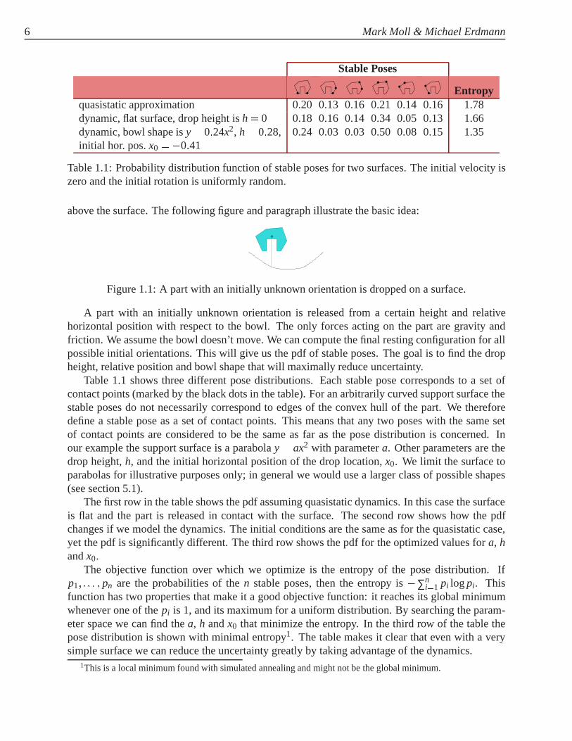
above the surface. The following figure and paragraph illustrate the basic idea:

��

��

Figure 1.1: A part with an initially unknown orientation is dropped on a surface.

A part with an initially unknown orientation is released from a certain height and relativehorizontal position with respect to the bowl. The only forces acting on the part are gravity andfriction. We assume the bowl doesn’t move. We can compute the final resting configuration for allpossible initial orientations. This will give us the pdf of stable poses. The goal is to find the dropheight, relative position and bowl shape that will maximally reduce uncertainty.

Table 1.1 shows three different pose distributions. Each stable pose corresponds to a set ofcontact points (marked by the black dots in the table). For an arbitrarily curved support surface thestable poses do not necessarily correspond to edges of the convex hull of the part. We thereforedefine a stable pose as a set of contact points. This means that any two poses with the same setof contact points are considered to be the same as far as the pose distribution is concerned. Inour example the support surface is a parabolay= ax2 with parametera. Other parameters are thedrop height,h, and the initial horizontal position of the drop location,x0. We limit the surface toparabolas for illustrative purposes only; in general we would use a larger class of possible shapes(see section 5.1).

The first row in the table shows the pdf assuming quasistatic dynamics. In this case the surfaceis flat and the part is released in contact with the surface. The second row shows how the pdfchanges if we model the dynamics. The initial conditions are the same as for the quasistatic case,yet the pdf is significantly different. The third row shows the pdf for the optimized values fora, handx0.

The objective function over which we optimize is the entropy of the pose distribution. Ifp1; : : : ; pn are the probabilities of then stable poses, then the entropy is�∑n

i=1 pi logpi . Thisfunction has two properties that make it a good objective function: it reaches its global minimumwhenever one of thepi is 1, and its maximum for a uniform distribution. By searching the param-eter space we can find thea, h andx0 that minimize the entropy. In the third row of the table thepose distribution is shown with minimal entropy1. The table makes it clear that even with a verysimple surface we can reduce the uncertainty greatly by taking advantage of the dynamics.

1This is a local minimum found with simulated annealing and might not be the global minimum.

Manipulation of Pose Distributions 7

1.2 Outline

In section 3 we will briefly go over the physical model and in particular the way we model colli-sions. In section 4 we will explain the notion of capture regions and introduce an extension andrelaxation of this notion in the form of so-called quasi-capture regions. Both the physical modeland these quasi-capture regions allow for fast computation of the pose distribution. In section 5we will present our simulation and experimental results. Finally, in section 6 we will discuss theresults presented in this report. But first we will give an overview of related work in the nextsection.

2 Related Work

2.1 Parts Feeding and Orienting

One of the most comprehensive works on the design of parts feeding and assembly designis (Boothroyd et al., 1982), which describes vibratory bowls as well as non-vibratory parts

feeders in detail. The APOS parts feeding system is described by Hitakawa (1988). It is part ofthe automatic assembly system called SMART (Sony Multi-Assembly Robot Technology). Oneof the strong points of the APOS system is its flexibility: by replacing the tray and fine-tuning thevibrating motion, other parts can be oriented.How these trays are designed andhowto change themotion is not clear. Automating this step would increase the flexibility even further.

Berkowitz and Canny (1996, 1997) used dynamic simulation to design a sequence of gatesfor a vibratory bowl. They represented the effects produced by the gates as state transitions in anon-deterministic state automaton. The dynamics were simulated with Mirtich’s impulse-baseddynamic simulator,Impulse(Mirtich and Canny, 1995). Christiansen et al. (1996) used geneticalgorithms to design a near-optimal sequence of gates for a given part. Optimality is defined interms of throughput. Here, the behavior of each gate is assumed to be known. So, in a sense(Christiansen et al., 1996) is complementary to (Berkowitz and Canny, 1997): the latter focuses onmodeling the behavior of gates, the former finds an optimal sequence of gates given their behavior.Akella et al. (1997) introduced a technique for orienting planar parts on a conveyor belt with a onedegree-of-freedom (DOF) manipulator. Here, it was assumed that the initial orientation is known.Lynch (1999) extended this idea to 3D parts on a conveyor belt with a twoDOF manipulator.Wiegley et al. (1996) presented a complete algorithm for designing passive fences to orient parts.Here, the initial orientation is unknown.

Goldberg (1993) showed that it is possible to orient polygonal parts with a frictionless parallel-jaw gripper without sensors. Goldberg conjectured and Chen and Ierardi (1995) proved that foreveryn-sided polygonal part, a sequence of ‘squeezes’ can be computed inO(n2) time that willorient it up to symmetry. The length of such a sequence isO(n). These results might have ana-logues in three dimensions. Marigo et al. (1997) showed how to orient and position a polyhedralpart by rolling it between the two hands of a parallel-jaw gripper. Here, however, infinite frictionis assumed, whereas Goldberg assumed no friction.

In (Rao et al., 1995) an algorithm is described to orient polyhedral parts using so-called pivotgrasps. A part is grasped with two hard finger contacts and is then free to rotate around the axisformed by the contacts. Their algorithm computes anm�m matrix of pivot grasps, wherem isthe number of stable configurations and each entry corresponds to a transition from one stableconfiguration to another. In general, there will be some null entries in this matrix. In other words,it is not always possible to go from any stable configuration to any other. A vision system is used

8


to determine a part’s location and orientation. In (Gudmundsson and Goldberg, 1997) a similarsystem is described, where a robot arm picks up parts that pass on a conveyor belt, but here thefocus is on tuning the speed of the conveyor belt. Gudmundsson and Goldberg analytically showhow to maximize throughput as a function of the speed of the conveyor belt.

Erdmann and Mason (1988) developed a tray-tilting sensorless manipulator that can orientplanar parts in the presence of friction. If it isn’t possible to bring a part into a unique orientation,the planner would try to minimize the number of final orientations. In (Erdmann et al., 1993) itis shown how (with some simplifying assumptions) three-dimensional parts can be oriented usinga tray-tilting manipulator. In particular, for polyhedral parts withn faces a sequence of ‘tilts’ oflengthO(n) can be found inO(n3) time. Zumel (1997) used a variation of the tray tilting idea toorient planar parts. Zumel used two actuated arms connected at a hinge to tilt parts from one armto the other. The stable poses of the part at different angles were pre-computed. The planner thenfound a sequence of joint angle pairs for the two arms that would orient the part.

In recent years a lot of work has been done on programmable force fields to orient parts(Bohringer et al., 1997, 1999; Kavraki, 1997). The idea is that using some kind of force ‘field’(implemented using e.g. MEMS actuator arrays) can be used to push the part in a certain orien-tation. Kavraki (1997) presented a vector field that induced two stable configurations for mostparts. Bohringer et al. used Goldberg’s algorithm (1993) to define a sequence of ‘squeeze fields’to orient a part. They also gave an example how programmable vector fields can be used to simul-taneously sort different parts and orient them. Luntz et al. (1997) implemented a parcel transportand manipulation system using a distributed actuator array borrowing ideas from B¨ohringer et al.

2.2 Stable Poses

To compute the stable poses of an object quasistatic dynamics is often assumed. Furthermore,usually it is assumed that the part is in contact with a flat surface and is initially at rest. Boothroydet al. (1972) were among the first to analyze this problem. Using potential energy arguments andsome simplifying assumptions they were able to get good approximations of the pdf’s of someparts. They also introduced a method to get a static solution for the pdf: the probability of comingto rest on a face is simply proportional to the area of the face’s projection on a sphere centered atthe center of mass. The probability of an unstable face is added to the probability of the face towhich it rolls. AnO(n2) algorithm forn-sided polyhedrons, based on this idea, was implementedby Wiegley et al. (1992). Mirtich et al. (1996) improve this method by approximating some of thedynamic effects. In particular, they compute the area of the intersection of a face with a unit-areacircle centered around the center of mass projected on the plane defined by that face. This is thentaken as a measure of stability for that face.

Kriegman (1997) introduced the notion of acapture region: a region in configuration spacesuch that any initial configuration in that region will converge to one final configuration. He alsodescribed an algorithm based on Morse theory that computes the maximal capture regions of anobject. Note that this work doesn’t assume quasistatic dynamics; as long as the part is initiallyat rest and in contact, and the dynamics in the system are dissipative, the capture regions will becorrect. The capture regions will in general not cover the entire configuration space.

Much work has also been done on determining the stable orientations of assemblies (Masonet al., 1997; Trinkle et al., 1995; Mattikalli et al., 1994). Here, an object is typically in contact with


several controlled rigid bodies (e.g., manipulators). Usually the only force acting on the object isgravity. In other words, this is not the same problem as determining whether we have form- orforce-closure. Mason et al. (1997) noted that results in this area are also applicable to locomotionof multi-legged robots over uneven terrain.

2.3 Collision and Contact Analysis

Computing reaction forces for an object in contact with a surface is far from trivial. In fact, Baraff(1993) showed that deciding whether a configuration with dynamic friction is consistent isNP-complete (in terms of the number of contact points). Erdmann (1994) introduced the generalizedfriction cone, which embeds the force constraints that define the Coulomb friction cone into thepart’s configuration space. The possible motions have a simple geometric interpretation with thisrepresentation. Another geometric approach to analyze multiple frictional contacts was proposedby Brost and Mason (1989). Their approach is limited to two dimensions (however, the configu-ration space is three-dimensional). It represents forces in a dual space as points. A friction conethen reduces to a line segment in the dual space, and the dual of multiple friction cones is a convexpolygon. Trinkle and Zeng (1995) developed a model to predict the quasistatic motion of a planarpart in multiple contact. Their analysis yields inequalities defining regions in the space of frictioncoefficients for which a particular contact mode (i.e., sliding, rolling, separating or a combinationthereof) is feasible. Related to this is the work of Wang and Mason (1987). They introduced animpact space, defined as all combinations of orientation and contact motion direction. Within thisspace one can analytically identify the areas that correspond to the different contact modes.

For rigid body collisions several models have been proposed. Many of these models are ei-ther too restrictive (e.g., Routh’s model (1897) constrains the collision impulse too much) or allowphysically impossible collisions (e.g., Whittaker’s model (1944) can predict arbitrarily high in-creases of system kinetic energy). Recently, Chatterjee and Ruina (1998) proposed a new collisionrule, which avoids many of these problems. Chatterjee introduced a new collision parameter (be-sides the coefficients of friction and restitution): the coefficient oftangentialrestitution. With thisextra parameter a large part of allowable collision impulses can be accounted for, and at the sametime this collision rule restricts the predicted collision impulse to the allowable part of impulsespace. This is the collision rule we will use.

Instead of having algebraic laws, one could also try to model object interactions during impact.This approach is, for instance, taken by Bhatt and Koechling (1995a,b), who modeled impacts as aflow problem. While this might lead to more accurate predictions, it is obviously computationallymore expensive. Also, in order to get a good approximation of the pdf of resting configurations,this level of accuracy might not be required. On the other hand, it is also possible to combine theeffects of multiple collisions that happen almost instantaneously. Goyal et al. (1998a,b) studiedthese “clattering” motions and derived the equations of motion for this class of motions.

Given a collision model and the equations of motion, one can simulate the motion of a part.Most of the complexity in dynamic simulation is due to collision detection. Using a particularquaternion representation for orientation, Canny (1986) reduced the problem of finding the distancebetween polyhedrons to finding the distance between a point and a number of hyperplanes in 7dimensions. Lin and Canny (1991) designed a fast algorithm to incrementally find the closestpoint between two convex polyhedra. In cases where there are a large number of collisions or


with contact modes that change frequently one can simulate the dynamics using so-called impulse-based simulation (Mirtich and Canny, 1995). However, there are limits to what systems one cansimulate. Under certain conditions the dynamics become chaotic (B¨uhler and Koditschek, 1990;Feldberg et al., 1990; Kechen, 1990). We are mostly interested in systems that arenot chaotic, butwhere the dynamics can not be modeled with a quasistatic approximation. In section 5.1 a numberof ‘chaos plots’ are shown that are very similar to the one in (Kechen, 1990).

2.4 Shape Design

The shape of an object and its environment imposes constraints on the possible motions of thatobject. Caine (1993) presented a method to visualize these motion constraints, which can be use-ful in the design phase of both part and manipulator. In (Krishnasamy, 1996) the mechanics ofentrapment were analyzed. That is, Krishnasamy discussed conditions for a part to “get trapped”and “stay trapped” in an extrusion, in the context of the APOS parts feeder. Sanderson (1984) pre-sented a method to characterize the uncertainty in position and orientation of a part in an assemblysystem. This method takes into account the shape of both part and assembly system.

In (Lynch et al., 1998) the optimal manipulator shape and motion were determined for a partic-ular part. The problem here was not to orient the part, but to perform a certain juggler’s skill (the“butterfly”). With a suitable parametrization of the shape and motion of the manipulator, a solutionwas found for a disk-shaped part that satisfied their motion constraints. Examples of these con-straints were: (1) the part cannot break contact, and (2) the part must always be rolling. Althoughthe analysis focused just on the juggling task, it shows that one can simulate and optimize dynamicmanipulation tasks using a suitable parametrization of manipulator (or surface) shape and motion.

3 Physical Model

To compute the pose distribution of an object, we need to model the dynamics. Since weare interested in a whole class of pose distributions (defined by the surface shape parameters

and drop location), it is important that we can compute these pose distributions for a given objectquickly. That is, within the class of interest we would like to quickly find the parameter settings thatresult in a pose distribution with the smallest entropy. Below we will state our other assumptionsregarding the physical model.

Let ρ be the radius of gyration andθ be the relative orientation of the contact point with respectto the center of mass. Then it will turn out to be useful to model the dynamics using the generalizedcoordinates(x;y;q), where(x;y) is the position of the center of mass andq= ρθ represents theorientation of the object. Using these particular generalized coordinates some equations are greatlysimplified. For example, the kinetic energy can then be written as

KE = 12m�v2

x+v2y+ρ2ω2�= 1

2mkvk2:

3.1 Collisions

Collisions are modeled using Chatterjee’s collision rule (Chatterjee and Ruina, 1998). This rulecomputes a collisional impulse that guarantees a non-negative dissipation of kinetic energy, non-interpenetration between colliding objects and a non-negative normal impulse. Furthermore, thecollisional impulse is restricted to lie on the surface or inside the friction cone. Since it is an alge-braic collision rule, the post-collision velocity can be computed quickly. The collisional impulseis a linear combination of two base impulses:

p1 =� nTvpren

nTM�1n;

p2 =�Mvpre;

wheren is the contact normal,M is the local mass matrix at the contact point andvpre is the relativepre-collision velocity in the work space between the objects at the contact point. In the general caseM will depend on the mass properties of both objects. However, if one of the objects is consideredimmobile (i.e., has infinite mass), it will only depend on the pose and mass distribution of the otherobject. In our case we consider the surface to be immobile. How to compute mass matrices in thegeneral case is described in e.g. (Smith, 1991). The ‘candidate’ collisional impulse is defined as

p = (1+e)p1+(1+et)(p2�p1);

12


wheree is the coefficient of restitution andet the coefficient of tangential restitution. This newparameteret gives us an extra parameter to model collisions without violating any physical con-straints. The coefficient of tangential restitution can range from�1 to 1. In case the candidateimpulse lies outside the (real space) friction cone, we project the candidate impulse onto the sur-face of the friction cone. The collisional impulse then becomes

p = (1+e)p1+λ(p2�p1); where

λ =µ(1+e)nTp1

kp2� (nTp2)nk�µnT(p2�p1):

As usual,µ denotes the coefficient of (dry sliding) friction. We assume that the coefficient of staticfriction is equal toµ. If the candidate impulse lies on or inside the friction cone, then the collisionalimpulsep is simply equal top. The collisional impulse in generalized coordinates is then equal to

pg =

�p

r�pρ

�= Fp; where

r = R

�cosθsinθ

�

F =

0@ 1 0

0 1�R

ρ sinθ Rρ cosθ

1A :

Note thatFT is just a transformation of generalized coordinates to world-space coordinates. Usingthe method described in (Smith, 1991) the mass matrix for our generalized coordinates simplifiesto M = m(FTF)�1, wherem is the mass of the object andM is 2�2 matrix.

Let the pre-collision velocity (in configuration space) bevi . We can then write the post-collisionvelocity (in configuration space) as

v f = vi +Fpm

:

Between collisions the only force acting on the part is gravity.

3.2 Rolling Contact

Rolling contact is modeled as a compound pendulum (see e.g. (Symon, 1971, p. 216) for details).The differential equation that describes the rotation around the contact point is

θ =grc

ρ2c

sinθ;

whererc is the distance between the center of mass and the contact point andρc is the radius ofgyration about the contact point. It can be shown thatρ2

c = ρ2+ r2c. We can numerically solve this

differential equation and check whether the part can maintain rolling contact.


3.3 Sliding Contact

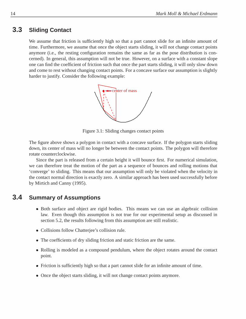
We assume that friction is sufficiently high so that a part cannot slide for an infinite amount oftime. Furthermore, we assume that once the object starts sliding, it will not change contact pointsanymore (i.e., the resting configuration remains the same as far as the pose distribution is con-cerned). In general, this assumption will not be true. However, on a surface with a constant slopeone can find the coefficient of friction such that once the part starts sliding, it will only slow downand come to rest without changing contact points. For a concave surface our assumption is slightlyharder to justify. Consider the following example:

center of mass

Figure 3.1: Sliding changes contact points

The figure above shows a polygon in contact with a concave surface. If the polygon starts slidingdown, its center of mass will no longer be between the contact points. The polygon will thereforerotate counterclockwise.

Since the part is released from a certain height it will bounce first. For numerical simulation,we can therefore treat the motion of the part as a sequence of bounces and rolling motions that‘converge’ to sliding. This means that our assumption will only be violated when the velocity inthe contact normal direction is exactly zero. A similar approach has been used successfully beforeby Mirtich and Canny (1995).

3.4 Summary of Assumptions

� Both surface and object are rigid bodies. This means we can use an algebraic collisionlaw. Even though this assumption is not true for our experimental setup as discussed insection 5.2, the results following from this assumption are still realistic.

� Collisions follow Chatterjee’s collision rule.

� The coefficients of dry sliding friction and static friction are the same.

� Rolling is modeled as a compound pendulum, where the object rotates around the contactpoint.

� Friction is sufficiently high so that a part cannot slide for an infinite amount of time.

� Once the object starts sliding, it will not change contact points anymore.

4 Analytic Results

4.1 Quasi-Capture Intuition

In our efforts to analyze pose distributions in a dynamic environment, we have been workingon a generalization of so-called ‘capture regions’ (Kriegman, 1997) that we have termedquasi-

capture regions. Specifically, for a part in contact with a sloped surface, we would like to determinewhether it is captured, i.e., whether the part will converge to the closest stable pose. For simplicity,let the surface be a tilted plane.

Definition 1. Let aposebe defined as a point in configuration space such that the part is in contactwith the surface.

We assume that friction is sufficiently high so that a part cannot slide for an infinite amount oftime. In general capture depends on the whole surface and everything that happens after the currentstate, but the friction assumption and our definition of pose allow us to define quasi-capture of thepart in terms of local state. The closest stable pose can be defined as follows:

Definition 2. We define astable poseto be a pose such that there is force balance when onlygravity and contact forces are acting on the part. Theclosest stable poseis the stable pose foundby following the gradient of the potential energy function (using e.g. gradient descent) from thecurrent pose.

We can now define quasi-capture regions:

Definition 3. A quasi-capture regionis the largest possible region in configuration phase spacesuch that (a) all configurations in this region have the same closest stable pose and (b) no con-figuration in a quasi-capture region has enough (kinetic and potential) energy to leave this regioneither with a rolling motion or one collision-free motion.

Ideally these quasi-capture regions would induce a partition of configuration phase space, sothat for each point in phase space we would immediately know what its final resting configurationis. Of course, this is not the case in general, since with a sufficiently large velocity an objectcan reach any stable pose. But if we restrict the velocity to be small to begin with, then we areable to quickly determine the pose distribution. It has been our experience that without the use ofquasi-capture regions a lot of computation time is spent on the final part/surface interactions (e.g,clattering motions) before the part reaches a stable pose. In other words,with our analytic resultsit is possible to avoid computing a potentially large number of collisions.

In section 3.3 we gave an example where sliding would change the final resting pose. Thenumerical approach we gave there showed that our assumption is still usable. A different approach

15


would be to shrink the quasi-capture regions by some amount to allow for some sliding. The exactamount can be computed numerically.

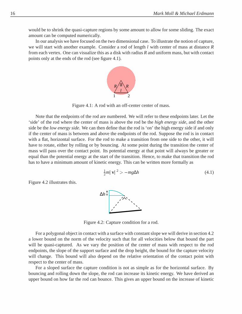
In our analysis we have focused on the two dimensional case. To illustrate the notion of capture,we will start with another example. Consider a rod of lengthl with center of mass at distanceRfrom each vertex. One can visualize this as a disk with radiusRand uniform mass, but with contactpoints only at the ends of the rod (see figure 4.1).

1 2

R Rαl

Figure 4.1: A rod with an off-center center of mass.

Note that the endpoints of the rod are numbered. We will refer to these endpoints later. Let the‘side’ of the rod where the center of mass is above the rod be thehigh energy side, and the otherside be thelow energy side. We can then define that the rod is ‘on’ the high energy side if and onlyif the center of mass is between and above the endpoints of the rod. Suppose the rod is in contactwith a flat, horizontal surface. For the rod to make a transition from one side to the other, it willhave to rotate, either by rolling or by bouncing. At some point during the transition the center ofmass will pass over the contact point. Its potential energy at that point will always be greater orequal than the potential energy at the start of the transition. Hence, to make that transition the rodhas to have a minimum amount of kinetic energy. This can be written more formally as

12mkvk2 >�mg∆h (4.1)

Figure 4.2 illustrates this.

h∆

Figure 4.2: Capture condition for a rod.

For a polygonal object in contact with a surface with constant slope we will derive in section 4.2a lower bound on the norm of the velocity such that for all velocities below that bound the partwill be quasi-captured. As we vary the position of the center of mass with respect to the rodendpoints, the slope of the support surface and the drop height, the bound for the capture velocitywill change. This bound will also depend on the relative orientation of the contact point withrespect to the center of mass.

For a sloped surface the capture condition is not as simple as for the horizontal surface. Bybouncing and rolling down the slope, the rod can increase its kinetic energy. We have derived anupper bound on how far the rod can bounce. This gives an upper bound on the increase of kinetic


energy. So the capture condition can now be stated as: the current kinetic energy plus the maximumgain in kinetic energy has to be less than the energy required to rotate to the other side. To guaranteethat the rod is indeed captured, we have to make sure that the maximum gain in kinetic energy isless than the decrease in kinetic energy due to a collision. There are some additional complicatingfactors. For instance, a change in orientation can increase the kinetic energy, but to rotate to theother side the rod has to rotate back, undoing the gain in kinetic energy.

4.2 Quasi-Capture Velocity

What we will prove is a sufficient condition on the pose and velocity of the rod such that it isquasi-captured on the titled plane. The condition will be of the following form: if the currentkinetic energy plus the maximal increase in kinetic energy is less than some bound, the rod isquasi-captured. This bound depends on the current orientation, the current velocity, the slope ofthe surface and the geometry of the rod. Because of the way we have set up our generalizedcoordinates, the kinetic energy is12mkvk2. In other words, the mass is just a constant scalar.Without loss of generality we can assumem= 2. That way the kinetic energy is simplykvk2. Wewill write v for kvk.Definition 4. Let a bounce be defined as the flight path between two impacts.

The closest distance between the rod and the slope during one bounce can be described by

d(t) = 12g(cosφ)t2+(vycosφ+vxsinφ)t�dθ(t); (4.2)

wherevx and vy are the translational components of the velocity anddθ(t) is a component thatdepends on the orientation. Let the rod be in contact att = 0. Thend(0) = 0 (and thereforedθ(0) = 0). Let t be the smallest positive solution tod(t) = 0. The change in height is then∆h= 1

2gt2+vyt, so that the change inv2 is ∆v2 = 2g∆h= g2t2+2vygt. To find the maximum∆v2

for all velocity vectors of lengthv we can parametrize the translational velocity asvx = vcosξ andvy = vsinξ, and maximize overξ. This ignores the rotational component of the velocity, but thefollowing lemma shows that for a certain value ofdθ(t) the resulting solution for∆v2 is an upperbound for the true maximal increase ofv2.

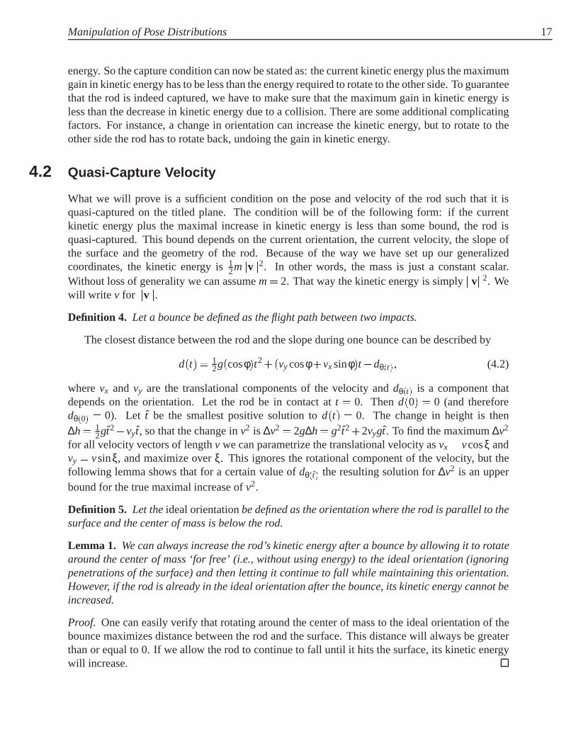
Definition 5. Let theideal orientationbe defined as the orientation where the rod is parallel to thesurface and the center of mass is below the rod.

Lemma 1. We can always increase the rod’s kinetic energy after a bounce by allowing it to rotatearound the center of mass ‘for free’ (i.e., without using energy) to the ideal orientation (ignoringpenetrations of the surface) and then letting it continue to fall while maintaining this orientation.However, if the rod is already in the ideal orientation after the bounce, its kinetic energy cannot beincreased.

Proof. One can easily verify that rotating around the center of mass to the ideal orientation of thebounce maximizes distance between the rod and the surface. This distance will always be greaterthan or equal to 0. If we allow the rod to continue to fall until it hits the surface, its kinetic energywill increase.


1

θ

-R

φcos(

αR

R

2

1

R α/2)

ideal

initial

sin(θ+φ)

(a) Change in distance between the cen-ter of mass and the surface in poses withthe initial and ideal orientation

dn= Rcos(α/2)-R

ideal

initial

sin(θ+φ)

(b) Trajectory of the center of mass during a bounce

Figure 4.3: Increase in kinetic energy when rotating to the ideal orientation

From this lemma it follows that by assuming the rod rotates to the ideal orientation the increase inkinetic energy due to one bounce is an upper bound on the true increase of kinetic energy. Withthis lemma computing the next contact point is a lot easier. Letθ be the relative orientation of thecontact point att = 0. θ = 0 corresponds to the contact point being to the right of the center ofmass. The signed distance from the center of mass to the surface att = 0 is then�Rsin(θ+ φ),as shown in figure 4.3(a). One can easily verify that in the ideal orientation the relative orientationof endpoint 1 isπ

2� α2 � φ. Let θ be equal to this relative orientation. In the pose where the rod

is in contact with the surface and has the ideal orientation the signed distance from the center ofmass to the surface is�Rsin(θ+φ) = �Rcosα

2 . So in total the center of mass travels a distanceR(cosα

2 �sin(θ+φ)) in the direction normal to the surface during one bounce. Letdn be equal tothis distance. To solve for the time of impact we can treat the rod as a point mass centered at thecenter of mass and replacedθ(t) in equation 4.2 with�dn. Equation 4.2 is then simply a paraboloidin t. The distance function now measures the distance between the center of mass and the dottedline parallel to the surface shown in figure 4.3(b). This approach is not limited to the case whereour new orientation is the ideal orientation. Suppose an oracle would tell us that the new orientationis θ. Then we can solve for the time of impact by substitutingR(sin(θ+φ)� sin(θ+φ)) for dθ(t)in equation 4.2.

The following lemma gives a bound on the velocity needed toroll to the other side.

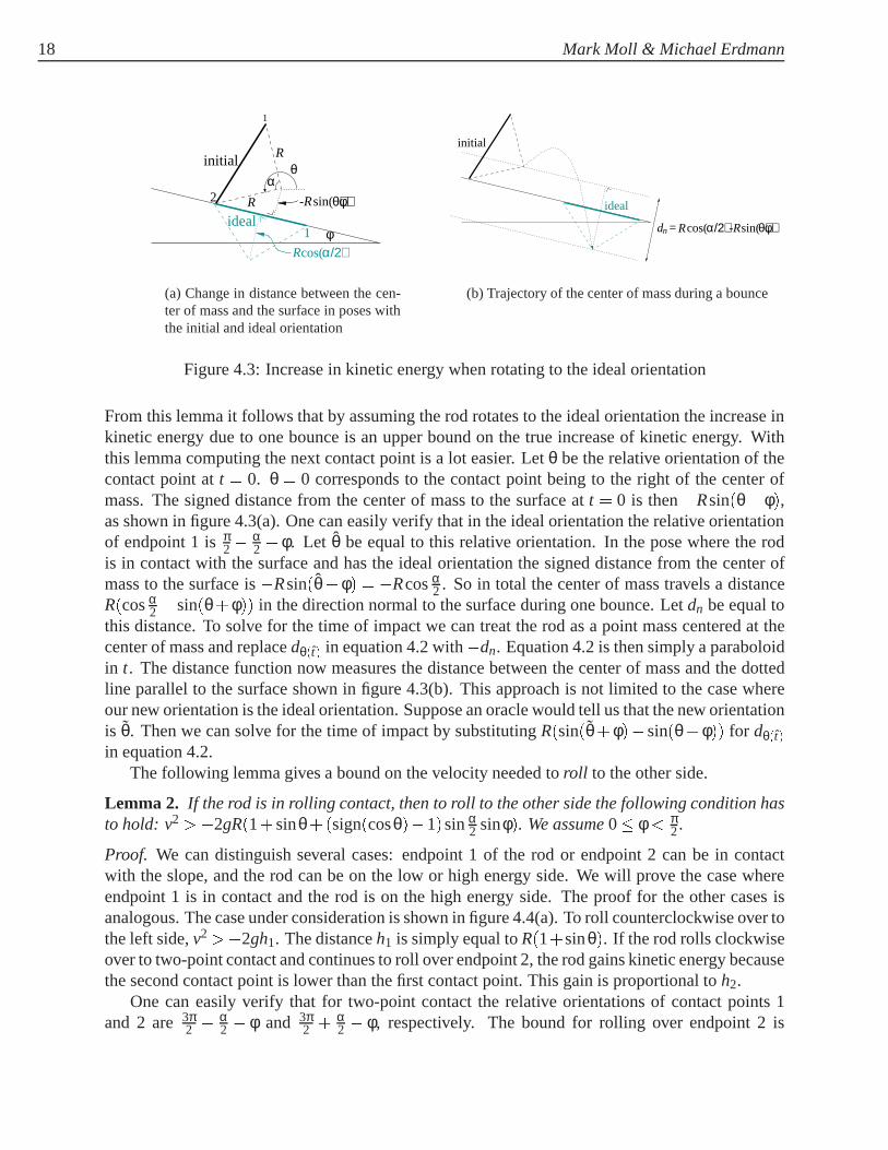
Lemma 2. If the rod is in rolling contact, then to roll to the other side the following condition hasto hold: v2 >�2gR(1+sinθ+(sign(cosθ)�1)sinα

2 sinφ). We assume0� φ < π2.

Proof. We can distinguish several cases: endpoint 1 of the rod or endpoint 2 can be in contactwith the slope, and the rod can be on the low or high energy side. We will prove the case whereendpoint 1 is in contact and the rod is on the high energy side. The proof for the other cases isanalogous. The case under consideration is shown in figure 4.4(a). To roll counterclockwise over tothe left side,v2 >�2gh1. The distanceh1 is simply equal toR(1+sinθ). If the rod rolls clockwiseover to two-point contact and continues to roll over endpoint 2, the rod gains kinetic energy becausethe second contact point is lower than the first contact point. This gain is proportional toh2.

One can easily verify that for two-point contact the relative orientations of contact points 1and 2 are3π

2 � α2 � φ and 3π

2 + α2 � φ, respectively. The bound for rolling over endpoint 2 is


φ

21h

hh3

θ

1

2

(a) Endpoint 1 in contact, high energyside

1hh3

φ

−θ

2

12h

(b) Endpoint 2 in contact, high energyside

h2

h3

1h

φθ1

2

(c) Endpoint 1 in contact, low energyside

h2

h3

1h

φ

θ

2

1

(d) Endpoint 2 in contact, low energyside

Figure 4.4: Capture condition for rotation

therefore

v2 >�2g(h3�h2)

=�2gR(1+sin(3π2 + α

2 �φ)�sin(3π2 � α

2 �φ)+sinθ)=�2gR(1+sinθ�cos(α

2 �φ)+cos(α2 +φ))

=�2gR(1+sinθ�2sinα2 sinφ):

If the center of mass is to the left of the contact point the last term will change sign. We cantherefore combine the two bounds (one for rotating clockwise, and for rotating counterclockwise)into this bound:

v2 > min��2gR(1+sinθ); �2gR(1+sinθ+2sign(cosθ)sinα

2 sinφ)�

=�2gR�1+sinθ+(sign(cosθ)�1)sinα

2 sinφ�: (4.3)


Theorem 1. The rod with a velocity vector of length v and in contact with the surface is in aquasi-capture region if the following condition holds:

v2+ 2vcosξsinφcos2φ

�vsin(ξ+φ)+

qv2sin2(ξ+φ)�2gdncosφ

��2g

�dn

cosφ +Rε�

��2gR�1+cos(α

2 +φ)�;

whereξ is the direction of the velocity vector that will result in the largest increase of kinetic

energy, dn = R(cosα2 �sin(θ+φ)) andε = cos(α

2 +φ)� cos(α=2)cosφ +max

�tanφ; 2sinα

2 sinφ�.

Proof. The path of the center of mass during a bounce that increases the kinetic energy maximallyis described by12gt2cosφ+ v(sinξcosφ+ cosξsinφ)t+dn = 0. The smallest positive solution ofthis equation is

t =�v(sinξcosφ+cosξsinφ)�

pv2(sinξcosφ+cosξsinφ)2�2gdn cosφgcosφ (4.4)

=�vsin(ξ+φ)�

pv2 sin2(ξ+φ)�2gdn cosφgcosφ :

The maximum change inv2 is then bounded by

∆v2 = 2g∆h

� 2g(12gt2+v(sinξ)t)

= 1cos2φ

�2v2sin2(ξ+φ)�2gdncosφ+2vsin(ξ+φ)


�

� 2vsinξcosφ

�vsin(ξ+φ)+


�

= 2vcosξsinφcos2 φ

�vsin(ξ+φ)+


�� 2gdn

cosφ : (4.5)

After one bounce the orientation is assumed to be such that rod is parallel to the surface and thecenter of mass is below the rod, as this will result in the largest increase in kinetic energy accordingto lemma 1. This means that endpoint 1’s relative orientation is equal toθ= π

2� α2�φ. Substituting

this value in equation 4.3 of lemma 2 gives�2gR(1+sinθ). In other words, if the kinetic energyafter the bounce is less than�2gR(1+sinθ) and the rod is in the ideal orientation, the rod cannotroll to the other side.

We can combine the two bounds to obtain a sufficient condition to determine whether the rodcan rotate to the other sideif its new orientation after one bounce is equal to the ideal orientation.Unfortunately this condition does not imply a similar condition for the general case where the neworientation is not necessarily equal to the ideal orientation.

Consider the casev= 0+. Substituting this value in equation 4.5 and expanding the definitionof dn shows that the maximum increase in kinetic energy is then

�2gdn

cosφ=�2gR(sin(θ+φ)�sin(θ+φ))

cosφ: (4.6)


Therefore, whenv= 0+ and the relative orientation of the contact point after the bounce is equalto ideal orientation the quasi-capture constraint is

�2gRsin(θ+φ)�sin(θ+φ)

cosφ��2gR(1+sinθ): (4.7)

That is, if an upper bound on the kinetic energy after one bounce is less than the energy needed torotate to the other side, the rod will not be able to rotate to the other side. Now suppose the neworientation isnot equal to the ideal orientation. Then the increase of kinetic energy will be less,but the energy required to roll to the other side will be less, too. Letθ be the relative orientation ofthe contact point after the bounce. Equation 4.7 is of the formf (θ)� g(θ), where f (�) computesthe kinetic energy after one bounce for a given new orientation andg(�) computes the energyneeded to roll to the other side for a given orientation1. Unfortunately, this bound does not imply8θ: f (θ) � g(θ). From the ‘oracle argument’ on page 18 it follows thatf (θ) is indeed an upperbound on the maximum increase of the kinetic energy. Substitutingθ in lemma 2 shows thatg(θ)is a lower bound on the kinetic energy needed to roll to the other side. We would like to determinethe smallest possibleε such that

f (θ)�2gRε� g(θ) ) 8θ: f (θ)� g(θ):

It is not hard to seeε has to be equal to maxθ(g(θ)�g(θ)� f (θ)+ f (θ))=(�2gR). The differencebetweenf (θ) and f (θ) is

�2gR(sin(θ+φ)�sin(θ+φ))cosφ +2gR(sin(θ+φ)�sin(θ+φ))

cosφ =�2gRsin(θ+φ)�sin(θ+φ)cosφ :

Similarly, the difference betweeng(θ) andg(θ) is

�2gR(1+sinθ)+2gR�1+sinθ+(sign(cosθ)�1)sinα

2 sinφ�

=�2gR�sinθ�sinθ� (sign(cosθ)�1)sinα

2 sinφ�:

The correctionε is therefore

ε = maxθ(sinθ�sinθ� (sign(cosθ)�1)sinα2 sinφ� sin(θ+φ)�sin(θ+φ)

cosφ )

By differentiating the expression inside max(�) with respect toθ we find that there is a local max-imum at θ = 0. Other local maxima occur whenθ approaches�π

2 from below or π2 from above.

The correctionε therefore simplifies to

ε = max�

sinθ� sin(θ+φ)�sinφcosφ ; sinθ+2sinα

2 sinφ� sin(θ+φ)cosφ

�

= cos(α2 +φ)� cos(α=2)

cosφ +max�tanφ; 2sinα

2 sinφ�:

Forv 6= 0+ the difference betweenf (θ) and f (θ) is even larger andg(θ) does not depend onv, sothe value forε is an upper bound for allv. Combining all the bounds we arrive at the following

1Analagous to expression 4.3,g(θ) equals�2gR�1+sinθ+(sign(cosθ)�1)sinα

2 sinφ�.


quasi-capture condition

v2+ 2vcosξsinφcos2φ

�vsin(ξ+φ)+


��2g

�dn

cosφ +Rε�

��2gR�1+cos(α

2 +φ)�:

Note that forφ = 0 this bound reduces tov2 � �2gR(1+ sinθ). In other words, this bound is astight as possible when the surface is horizontal.

For an arbitrarydn it is not possible to compute the optimalξ analytically. Fortunately, wecananalytically solve forξ if we assume that the bounce consists of pure translation. The resultingξcan be used as an approximation. To find this approximation we substitutedθ(t) = 0 in the distancefunction (equation 4.2):

d(t) =12

g(cosφ)t2+(vycosφ+vxsinφ)t:

The positive solution to this ist = �2(vy+vx tanφ)g . The change in height for the center of mass is

therefore

∆h=12

gt2+vyt

= 2gvx tanφ(vy+vx tanφ)

= 2gv2cosξ tanφ(sinξ+cosξ tanφ)

= 1gv2 tanφ(tanφ(1+cos(2ξ))+sin(2ξ)) :

To determine the most negative change in height, we differentiate with respect toξ and find itsroots

ddξ

∆h= 1gv2 tanφ(cos(2ξ)� tanφsin(2ξ)) = 0 ) cot(2ξ) = tanφ:

By checking the second derivative we can verify that this is indeed a minimum for 0� φ < π2. We

can rewrite the solution forξ as

cosξ =cosφp

2p

1�sinφ

sinξ =p

1�sinφp2

:

Substituting these values in equation 4.4, we find that the approximation for the bound for∆v2 thensimplifies to

∆v2��2gdn

cosφ+

v2sinφ1�sinφ

�1+

q1�4dng(1�sinφ)=(v2cosφ)

�


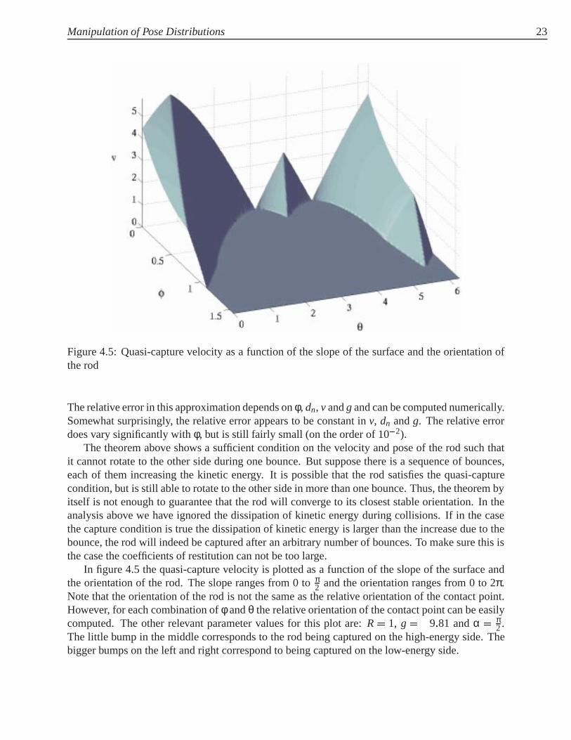
Figure 4.5: Quasi-capture velocity as a function of the slope of the surface and the orientation ofthe rod

The relative error in this approximation depends onφ, dn, v andg and can be computed numerically.Somewhat surprisingly, the relative error appears to be constant inv, dn andg. The relative errordoes vary significantly withφ, but is still fairly small (on the order of 10�2).

The theorem above shows a sufficient condition on the velocity and pose of the rod such thatit cannot rotate to the other side during one bounce. But suppose there is a sequence of bounces,each of them increasing the kinetic energy. It is possible that the rod satisfies the quasi-capturecondition, but is still able to rotate to the other side in more than one bounce. Thus, the theorem byitself is not enough to guarantee that the rod will converge to its closest stable orientation. In theanalysis above we have ignored the dissipation of kinetic energy during collisions. If in the casethe capture condition is true the dissipation of kinetic energy is larger than the increase due to thebounce, the rod will indeed be captured after an arbitrary number of bounces. To make sure this isthe case the coefficients of restitution can not be too large.

In figure 4.5 the quasi-capture velocity is plotted as a function of the slope of the surface andthe orientation of the rod. The slope ranges from 0 toπ

2 and the orientation ranges from 0 to 2π.Note that the orientation of the rod is not the same as the relative orientation of the contact point.However, for each combination ofφ andθ the relative orientation of the contact point can be easilycomputed. The other relevant parameter values for this plot are:R= 1, g= �9:81 andα = π

2.The little bump in the middle corresponds to the rod being captured on the high-energy side. Thebigger bumps on the left and right correspond to being captured on the low-energy side.

5 Simulations and Experiments

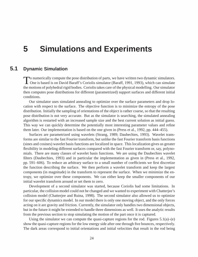
5.1 Dynamic Simulation

To numerically compute the pose distribution of parts, we have written two dynamic simulators.One is based is on David Baraff’s Coriolis simulator (Baraff, 1991, 1993), which can simulate

the motions of polyhedral rigid bodies. Coriolis takes care of the physical modelling. Our simulatorthen computes pose distributions for different (parametrized) support surfaces and different initialconditions.

Our simulator uses simulated annealing to optimize over the surface parameters and drop lo-cation with respect to the surface. The objective function is to minimize the entropy of the posedistribution. Initially the sampling of orientations of the object is rather coarse, so that the resultingpose distribution is not very accurate. But as the simulator is searching, the simulated annealingalgorithm is restarted with an increased sample size and the best current solution as initial guess.This way we can quickly determine the potentially most interesting parameter values and refinethem later. Our implementation is based on the one given in (Press et al., 1992, pp. 444–455).

Surfaces are parametrized using wavelets (Strang, 1989; Daubechies, 1993). Wavelet trans-forms are similar to the fast Fourier transform, but unlike the fast Fourier transform basis functions(sines and cosines) wavelet basis functions are localized in space. This localization gives us greaterflexibility in modeling different surfaces compared with the fast Fourier transform or, say, polyno-mials. There are many classes of wavelet basis functions. We are using the Daubechies waveletfilters (Daubechies, 1993) and in particular the implementation as given in (Press et al., 1992,pp. 591–606). To reduce an arbitrary surface to a small number of coefficients we first discretizethe function describing the surface. We then perform a wavelet transform and keep the largestcomponents (in magnitude) in the transform to represent the surface. When we minimize the en-tropy, we optimize over these components. We can either keep the smaller components of ourinitial wavelet transform around or set them to zero.

Development of a second simulator was started, because Coriolis had some limitations. Inparticular, the collision model could not be changed and we wanted to experiment with Chatterjee’scollision model (Chatterjee and Ruina, 1998). The second simulator also allowed us to optimizefor our specific dynamics model. In our model there is only one moving object, and the only forcesacting on it are gravity and friction. Currently, the simulator only handles two dimensional objects,but in the future it might be extended to handle three dimensions as well. It uses the analytic resultsfrom the previous section to stop simulating the motion of the part once it is captured.

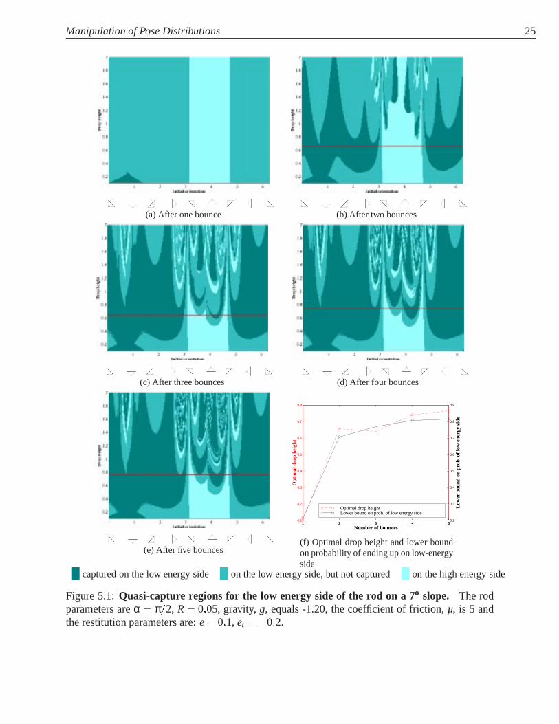
Using the simulator we can compute the quasi-capture regions for the rod. Figures 5.1(a)–(e)show the quasi-capture regions for the low energy side after one through five bounces, respectively.The dark areas correspond to initial orientations and initial velocities that result in the rod being

24


(a) After one bounce (b) After two bounces

(c) After three bounces (d) After four bounces

(e) After five bounces

1 2 3 4 50.1

0.2

0.3

0.4

0.5

0.6

0.7

0.8

Number of bounces

Opt

imal

dro

p he

ight

1 2 3 4 50.2

0.3

0.4

0.5

0.6

0.7

0.8

0.9

Low

er b

ound

on

prob

. of l

ow e

nerg

y si

de

Optimal drop height Lower bound on prob. of low energy side

(f) Optimal drop height and lower boundon probability of ending up on low-energyside

captured on the low energy side on the low energy side, but not captured on the high energy side

Figure 5.1:Quasi-capture regions for the low energy side of the rod on a 7o slope. The rodparameters areα = π=2, R= 0:05, gravity,g, equals -1.20, the coefficient of friction,µ, is 5 andthe restitution parameters are:e= 0:1, et =�0:2.


quasi-captured. The zero orientation is defined as the orientation where endpoint 1 is to the rightof the center of mass. The triangles below theX-axes show the pose of the rod corresponding tothe orientation at that point of theX-axes.

Let the optimal drop height be defined as the drop height that maximizes the probability ofending up on the low energy side. Then dropping the rod with uniformly random initial orientationfrom the optimal drop height will reduce uncertainty about its orientation maximally (unless thereexists a drop height that will result in an even higher probability for the high energy side). In figures5.1(a)–(e) the drop height that results in the maximum probability of ending up on the low energyside is marked by a horizontal line. After each successive bounce this drop height is likely to bea better approximation of the optimal drop height. In figure 5.1(f) the approximate optimal dropheight and lower bound on the probability of ending up on the low-energy side after one throughfive bounces is shown. One thing to note is that both the optimal drop height and the lower boundon the probability of ending up on low-energy side rapidly converge. This seems to suggest thatafter only a small number of bounces we could make a reasonable estimate of the optimal dropheight and uncertainty reduction. Further study is needed to find out if this is true in general.

5.2 2D Results

To verify the simulations we also performed some experiments. Our experimental setup was asfollows. We used an air table to effectively create a two-dimensional world. By varying the slopeof the air table we can vary the gravity. At the bottom of the slope is the surface on which theobject will be dropped. The angleφ of the surface in the plane defined by the air table can, ofcourse, be varied.

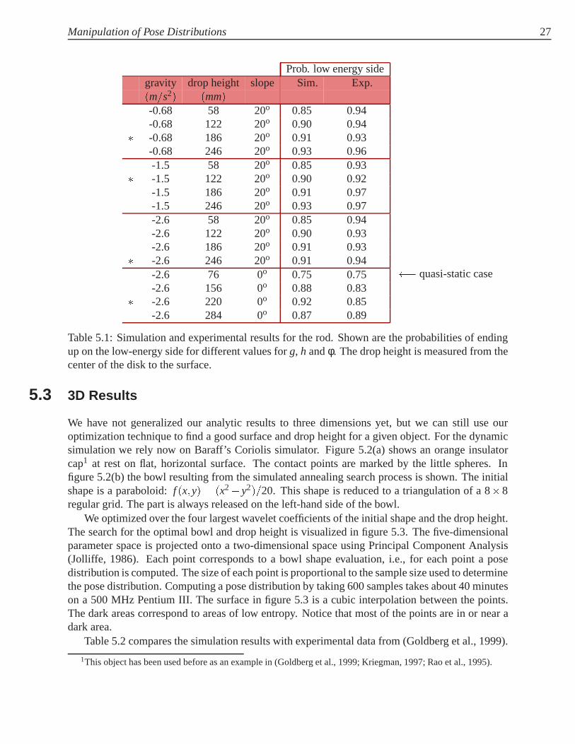
The rod of the previous section has been implemented as a plastic disk with two metal pinssticking out from the top at an equal distance from the center of the disk. When released fromthe top of the air table the disk can slide under the surface and will only collide at the pins. Ex-perimentally we determined the pose distribution of the rod for different values forg, h andφ bydetermining the final stable pose for 72 equally spaced initial orientations. Our simulation andexperimental results of some tests have been summarized in table 5.1. The rows marked with anasterisk have been used to estimate the moment of inertia of the rod and the coefficients of frictionand restitution. The estimated values for these parameters are:e= 0:404,et =�0:136,ρ= 0:0376andµ= 4:71. Note that for a low drop height and a horizontal surface (row 13 in table 5.1) the pdfis equal to a quasistatic approximation, as one would expect. More surprisingly, we see that theprobability of ending up on the low-energy side can be changed to approximately 0.95 by settingg, h andφ to appropriate values. In other words, we can reduce the uncertainty almost completely.

One can identify several error sources for the differences between the simulation and experi-mental results. First, there are measurement errors in the experiments: in some cases slight changesin the initial conditions will change the side on which the rod will end up. Second, since the sim-ulations are run with finite precision, it is possible that numerical errors affect the results. Finally,the physical model is not perfect. In particular, the rigid body assumption is just false. The surfaceon which the rod lands is coated with a thin layer of foam to create a high-damping, rough surface.This is done to prevent the rod from colliding with the sides of the air table.


Prob. low energy sidegravity drop height slope Sim. Exp.(m=s2) (mm)-0.68 58 20o 0.85 0.94-0.68 122 20o 0.90 0.94

� -0.68 186 20o 0.91 0.93-0.68 246 20o 0.93 0.96-1.5 58 20o 0.85 0.93

� -1.5 122 20o 0.90 0.92-1.5 186 20o 0.91 0.97-1.5 246 20o 0.93 0.97-2.6 58 20o 0.85 0.94-2.6 122 20o 0.90 0.93-2.6 186 20o 0.91 0.93

� -2.6 246 20o 0.91 0.94-2.6 76 0o 0.75 0.75-2.6 156 0o 0.88 0.83

� -2.6 220 0o 0.92 0.85-2.6 284 0o 0.87 0.89

� quasi-static case

Table 5.1: Simulation and experimental results for the rod. Shown are the probabilities of endingup on the low-energy side for different values forg, h andφ. The drop height is measured from thecenter of the disk to the surface.

5.3 3D Results

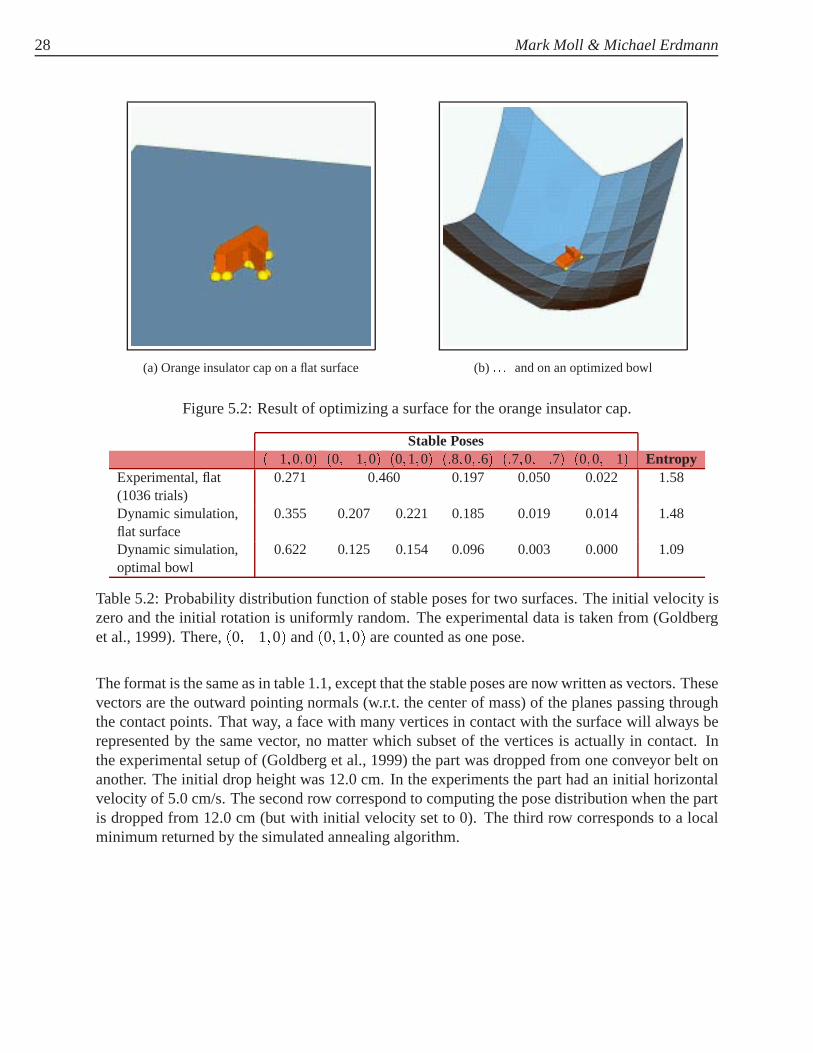
We have not generalized our analytic results to three dimensions yet, but we can still use ouroptimization technique to find a good surface and drop height for a given object. For the dynamicsimulation we rely now on Baraff’s Coriolis simulator. Figure 5.2(a) shows an orange insulatorcap1 at rest on flat, horizontal surface. The contact points are marked by the little spheres. Infigure 5.2(b) the bowl resulting from the simulated annealing search process is shown. The initialshape is a paraboloid:f (x;y) = (x2+ y2)=20. This shape is reduced to a triangulation of a 8�8regular grid. The part is always released on the left-hand side of the bowl.

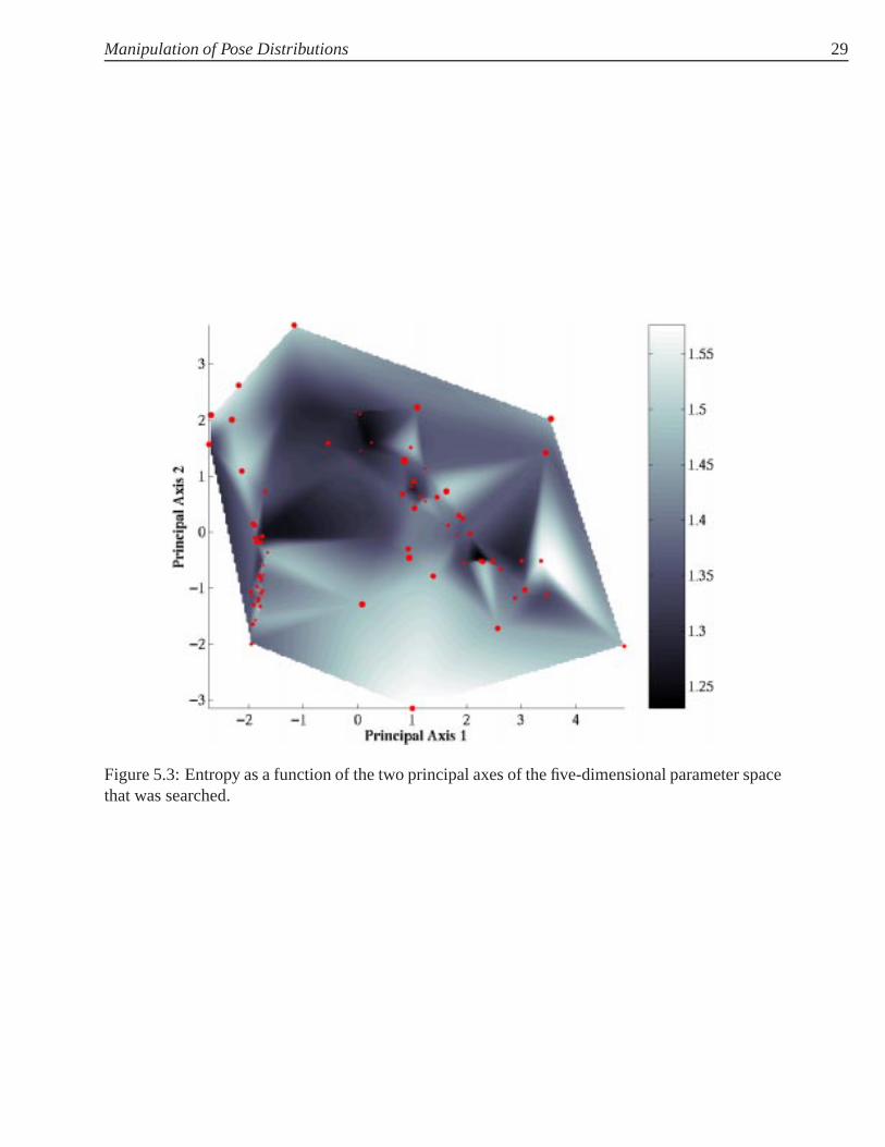
We optimized over the four largest wavelet coefficients of the initial shape and the drop height.The search for the optimal bowl and drop height is visualized in figure 5.3. The five-dimensionalparameter space is projected onto a two-dimensional space using Principal Component Analysis(Jolliffe, 1986). Each point corresponds to a bowl shape evaluation, i.e., for each point a posedistribution is computed. The size of each point is proportional to the sample size used to determinethe pose distribution. Computing a pose distribution by taking 600 samples takes about 40 minuteson a 500 MHz Pentium III. The surface in figure 5.3 is a cubic interpolation between the points.The dark areas correspond to areas of low entropy. Notice that most of the points are in or near adark area.

Table 5.2 compares the simulation results with experimental data from (Goldberg et al., 1999).

1This object has been used before as an example in (Goldberg et al., 1999; Kriegman, 1997; Rao et al., 1995).


(a) Orange insulator cap on a flat surface (b) : : : and on an optimized bowl

Figure 5.2: Result of optimizing a surface for the orange insulator cap.

Stable Poses(�1;0;0) (0;�1;0) (0;1;0) (:8;0; :6) (:7;0;�:7) (0;0;�1) Entropy

Experimental, flat(1036 trials)

0.271 0.460 0.197 0.050 0.022 1.58

Dynamic simulation,flat surface

0.355 0.207 0.221 0.185 0.019 0.014 1.48

Dynamic simulation,optimal bowl

0.622 0.125 0.154 0.096 0.003 0.000 1.09

Table 5.2: Probability distribution function of stable poses for two surfaces. The initial velocity iszero and the initial rotation is uniformly random. The experimental data is taken from (Goldberget al., 1999). There,(0;�1;0) and(0;1;0) are counted as one pose.

The format is the same as in table 1.1, except that the stable poses are now written as vectors. Thesevectors are the outward pointing normals (w.r.t. the center of mass) of the planes passing throughthe contact points. That way, a face with many vertices in contact with the surface will always berepresented by the same vector, no matter which subset of the vertices is actually in contact. Inthe experimental setup of (Goldberg et al., 1999) the part was dropped from one conveyor belt onanother. The initial drop height was 12.0 cm. In the experiments the part had an initial horizontalvelocity of 5.0 cm/s. The second row correspond to computing the pose distribution when the partis dropped from 12.0 cm (but with initial velocity set to 0). The third row corresponds to a localminimum returned by the simulated annealing algorithm.


Figure 5.3: Entropy as a function of the two principal axes of the five-dimensional parameter spacethat was searched.

6 Discussion

We have shown a sufficient condition on the position and velocity of the simplest possible‘interesting’ shape (i.e., the rod) that guarantees convergence to the nearest stable pose under

some assumptions. This condition gives rise to regions in configuration phase-space, where eachpoint within such a region will converge to the same stable pose. We have coined the term quasi-capture regions for these regions, since they are very similar to Kriegman’s notion of captureregions.

The quasi-capture regions also apply to general polygonal shapes. However, we can no longeruse the symmetry of the rod. So the quasi-capture expressions for general polygonal shapes be-come more complex. On the other hand, we might be able to orient planar parts by using a setupsimilar to the one described in section 5 and attaching two pins to the top of the part. Generalizingthe quasi-capture regions to three dimensions is non-trivial and is an interesting direction for futureresearch.

The simulation and experimental results show that the simulator is not 100% accurate, butthat it is a useful tool for determining the most promising initial conditions for uncertainty reduc-tion. In other words, the optimum predicted by the simulator will probably be near-optimal in theexperiments. We can then experimentally search for the true optimum.

Another area where quasi-capture regions may be applied is in computer animation. Before apart comes to rest, there are many interactions between the part and the support surface. It turnsout that these interactions are computationally very expensive. With our capture regions we caneliminate the last ‘clattering’ motions of the part, since we can predict what the final pose will be.For applications where fast animation is more important than physical accuracy, a pre-computedmotion can be substituted for the actual motion.

With future research we hope to improve the constraints on the quasi-capture velocity by tak-ing into account more information, such as the direction of the velocity vector. If improving thequasi-capture bounds is impossible, it might be possible to get better approximations for pose dis-tributions. As noted in section 5.1 it is possible to get a good estimate of the maximal uncertaintyreduction after only a small number of bounces of the rod. So another interesting line of researchwould be to find out how accurate these approximations are in general. We are also planning to domore experiments to verify our current and future analytic results.

30

References

Akella, S., Huang, W. H., Lynch, K. M., and Mason, M. T. (1997). Sensorless parts orienting witha one-joint manipulator. InProc. 1997 IEEE Intl. Conf. on Robotics and Automation.

Baraff, D. (1991). Coping with friction for non-penetrating rigid body simulation.ComputerGraphics, 25(4):31–40.

Baraff, D. (1993). Issues in computing contact forces for non-penetrating rigid bodies.Algorith-mica, pages 292–352.

Berkowitz, D. R. and Canny, J. (1996). Designing parts feeders using dynamic simulation. InProc. 1996 IEEE Intl. Conf. on Robotics and Automation, pages 1127–1132.

Berkowitz, D. R. and Canny, J. (1997). A comparison of real and simulated designs for vibratoryparts feeding. InProc. 1997 IEEE Intl. Conf. on Robotics and Automation, pages 2377–2382,Albuquerque, New Mexico.

Bhatt, V. and Koechling, J. (1995a). Partitioning the parameter space according to different behav-ior during 3d impacts.ASME Journal of Applied Mechanics, 62(3):740–746.

Bhatt, V. and Koechling, J. (1995b). Three dimensional frictional rigid body impact.ASME Journalof Applied Mechanics, 62(4):893–898.

Bohringer, K. F., Bhatt, V., Donald, B. R., and Goldberg, K. Y. (1997). Algorithms for sensorlessmanipulation using a vibrating surface.Algorithmica. Accepted for publication.

Bohringer, K. F., Donald, B. R., and MacDonald, N. C. (1999). Programmable vector fields fordistributed manipulation, with applications to MEMS actuator arrays and vibratory parts feeders.Intl. J. of Robotics Research, 18(2):168–200.

Boothroyd, C., Redford, A. H., Poli, C., and Murch, L. E. (1972). Statistical distributions of nat-ural resting aspects of parts for automatic handling.Manufacturing Engineering Transactions,Society of Manufacturing Automation, 1:93–105.

Boothroyd, G., Poli, C., and Murch, L. E. (1982).Automatic Assembly. Marcel Dekker, Inc., NewYork; Basel.

Brost, R. C. and Mason, M. T. (1989). Graphical analysis of planar rigid-body dynamics withmultiple frictional contacts. InFifth International Symposium on Robotics Research, pages293–300.

31


Buhler, M. and Koditschek, D. E. (1990). From stable to chaotic juggling: Theory, simulation, andexperiments. InProc. 1990 IEEE Intl. Conf. on Robotics and Automation, pages 1976–1981.

Caine, M. E. (1993).The Design of Shape from Motion Constraints. PhD thesis, MIT ArtificialIntelligence Laboratory, Cambridge, MA. Technical Report 1425.

Canny, J. (1986). Collision detection for moving polyhedra.IEEE Trans. on Pattern Analysis andMachine Intelligence, 8(2):200–209.

Chatterjee, A. and Ruina, A. L. (1998). A new algebraic rigid body collision law based on impulsespace considerations.ASME Journal of Applied Mechanics. Accepted for publication.

Chen, Y.-B. and Ierardi, D. (1995). The complexity of oblivious plans for orienting and distin-guishing polygonal parts.Algorithmica, 14.

Christiansen, A. D., Edwards, A. D., and Coello Coello, C. A. (1996). Automated design of partfeeders using a genetic algorithm. InProc. 1996 IEEE Intl. Conf. on Robotics and Automation,volume 1, pages 846–851.

Daubechies, I., editor (1993).Different Perspectives on Wavelets, volume 47 ofProceedings ofSymposia in Applied Mathematics. AMS.

Erdmann, M. A. (1994). On a representation of friction in configuration space.Intl. J. of RoboticsResearch, 13(3):240–271.

Erdmann, M. A. and Mason, M. T. (1988). An exploration of sensorless manipulation.IEEE J. ofRobotics and Automation, 4(4):369–379.

Erdmann, M. A., Mason, M. T., and Vanˇecek, Jr., G. (1993). Mechanical parts orienting: The caseof a polyhedron on a table.Algorithmica, 10:226–247.

Feldberg, R., Szymkat, M., Knudsen, C., and Mosekilde, E. (1990). Iterated-map approach to dietossing.Physical Review A, 42(8):4493–4502.

Goldberg, K., Mirtich, B., Zhuang, Y., Craig, J., Carlisle, B., and Canny, J. (1999). Part posestatistics: Estimators and experiments.IEEE Trans. on Robotics and Automation, 15(5).

Goldberg, K. Y. (1993). Orienting polygonal parts without sensors.Algorithmica, 10(3):201–225.

Goyal, S., Papadopoulos, J. M., and Sullivan, P. A. (1998a). The dynamics of clattering I: Equationof motion and examples.J. of Dynamic Systems, Measurement, and Control, 120:83–93.

Goyal, S., Papadopoulos, J. M., and Sullivan, P. A. (1998b). The dynamics of clattering II: Globalresults and shock protection.J. of Dynamic Systems, Measurement, and Control, 120:94–102.

Gudmundsson, D. and Goldberg, K. (1997). Tuning robotic part feeder parameters to maximizethroughput. InProc. 1997 IEEE Intl. Conf. on Robotics and Automation, pages 2440–2445,Albuquerque, New Mexico.


Hitakawa, H. (1988). Advanced parts orientation system has wide application.Assembly Automa-tion, 8(3):147–150.

Jolliffe, I. T. (1986).Principal Components Analysis. Springer-Verlag, New York.

Kavraki, L. E. (1997). Part orientation with programmable vector fields: Two stable equilibriafor most parts. InProc. 1997 IEEE Intl. Conf. on Robotics and Automation, pages 2446–2451,Albuquerque, New Mexico.

Kechen, Z. (1990). Uniform distribution of initial states: The physical basis of probability.PhysicalReview A, 41(4):1893–1900.

Kriegman, D. J. (1997). Let them fall where they may: Capture regions of curved objects andpolyhedra.Intl. J. of Robotics Research, 16(4):448–472.

Krishnasamy, J. (1996).Mechanics of Entrapment with Applications to Design of Industrial PartFeeders. PhD thesis, Dept. of Mechanical Engineering, MIT.

Lin, M. C. and Canny, J. F. (1991). A fast algorithm for incremental distance calculation. InProc.1991 IEEE Intl. Conf. on Robotics and Automation, pages 1008–1014, Sacramento, CA.

Luntz, J. E., Messner, W., and Choset, H. (1997). Parcel manipulation and dynamics with a dis-tributed actuator array: The virtual vehicle. InProc. 1997 IEEE Intl. Conf. on Robotics andAutomation, Albuquerque, New Mexico.

Lynch, K. M. (1999). Toppling manipulation. InProc. 1999 IEEE Intl. Conf. on Robotics andAutomation, pages 2551–2557, Detroit, MI.

Lynch, K. M., Shiroma, N., Arai, H., and Tanie, K. (1998). The roles of shape and motion indynamic manipulation: The butterfly example. InProc. 1998 IEEE Intl. Conf. on Robotics andAutomation.

Marigo, A., Chitour, Y., and Bicchi, A. (1997). Manipulation of polyhedral parts by rolling. InProc. 1997 IEEE Intl. Conf. on Robotics and Automation, pages 2992–2997.

Mason, R., Rimon, E., and Burdick, J. (1997). Stable poses of 3-dimensional objects. InProc.1997 IEEE Intl. Conf. on Robotics and Automation, pages 391–398.

Mattikalli, R., Baraff, D., and Khosla, P. (1994). Finding all gravitationally stable orientations ofassemblies. InProc. 1994 IEEE Intl. Conf. on Robotics and Automation.

Mirtich, B. and Canny, J. (1995). Impulse-based simulation of rigid bodies. InProc. 1995 Sympo-sium on Interactive 3D Graphics.

Mirtich, B., Zhuang, Y., Goldberg, K., Craig, J., Zanutta, R., Carlisle, B., and Canny, J. (1996).Estimating pose statistics for robotic part feeders. InProc. 1996 IEEE Intl. Conf. on Roboticsand Automation.

Press, W. H., Teukolsky, S. A., Vetterling, W. T., and Flannery, B. P. (1992).Numerical Recipes inC: The art of Scientific Computing. Cambridge University Press, second edition.


Rao, A., Kriegman, D., and Goldberg, K. (1995). Complete algorithms for reorienting polyhedralparts using a pivoting gripper. InProc. 1995 IEEE Intl. Conf. on Robotics and Automation.

Routh, E. J. (1897).Dynamics of a System of Rigid Bodies. MacMillan and Co., London, sixthedition.

Sanderson, A. C. (1984). Parts entropy methods for robotic assembly system design. InProc. 1984IEEE Intl. Conf. on Robotics and Automation, pages 600–608.

Smith, C. E. (1991). Predicting rebounds using rigid-body dynamics.ASME Journal of AppliedMechanics, 58:754–758.

Strang, G. (1989). Wavelets and dilation equations: A brief introduction.SIAM Review, 31:613–627.

Symon, K. R. (1971).Mechanics. Addison-Wesley, Reading, MA.

Trinkle, J. C., Farahat, A. O., and Stiller, P. F. (1995). First-order stability cells of active multi-rigid-body systems.IEEE Trans. on Robotics and Automation, 11(4):545–557.

Trinkle, J. C. and Zeng, D. C. (1995). Prediction of the quasistatic planar motion of a contactedrigid body. IEEE Trans. on Robotics and Automation, 11(2):229–246.

Wang, Y. and Mason, M. T. (1987). Modelling impact dynamics for robotic operations. InProc.1987 IEEE Intl. Conf. on Robotics and Automation, pages 678–685.

Whittaker, E. T. (1944).A Treatise on the Analytical Dynamics of Particles and Rigid Bodies.Dover, New York, fourth edition.

Wiegley, J., Goldberg, K., Peshkin, M., and Brokowski, M. (1996). A complete algorithm fordesigning passive fences to orient parts. InProc. 1996 IEEE Intl. Conf. on Robotics and Au-tomation.

Wiegley, J., Rao, A., and Goldberg, K. (1992). Computing a statistical distribution of stable posesfor a polyhedron. In30th Annual Allerton Conf. on Communications, Control and Computing.

Zumel, N. B. (1997).A Nonprehensile Method for Reliable Parts Orienting. PhD thesis, RoboticsInstitute, Carnegie Mellon University, Pittsburgh, PA.

Documents

Manipulation of Pose Distributionsreports-archive.adm.cs.cmu.edu/anon/anon/2000/CMU-CS-00-111.pdfManipulation of Pose Distributions Mark Moll Michael A. Erdmann March 11, 2000 CMU-CS-00-111