Embed Size (px)
Citation preview
Scheduling Dependent Real-Time Activities
Raymond Keith Clark
August 1990
CMU-CS-90-155
School of Computer Science
Carnegie Mellon University
Pittsburgh, Pennsylvania 15213
Submitted in partial fulfillment of the requirements
for the degree of Doctor of Philosophy in
Computer Science at Carnegie Mellon University
Copyright 1990 Raymond K. Clark
This research was supported in part by the USAF Rome Air Development Center (RADC) under contractnumber F30602-85-C-0274; in part by RADC under contract number F33602-88-D-0027, monitored by theCALSPAN-UB Research Center (CUBRC) as Subcontract C/UB-04; and in part by the ConcurrentComputer Corporation (CCUR). The views and conclusions contained in this document are those of theauthor and should not be interpreted as representing the official policies, either expressed or implied, ofRADC, CUBRC, CCUR, or the United States Government.

Keywords: Real-time systems, Scheduling and sequencing, Operating systems, Algorithms, Command
and control, Industrial control.

This work is dedicated tomy parents, Ellen and Ray,
and tomy wife, Rhonda,
all of whom have dedicated so much of their lives,and themselves,
to me.
Acknowledgments
A number of people deserve recognition for their contributions, both tangible and intangible, to this
thesis.
First of all, I must thank Doug Jensen. When I first encountered him, I saw that he was attempting to
solve real-time problems that were similar to some that I had confronted and which had fascinated me. He
allowed me to join the Archons Project at Carnegie Mellon in order to help solve these problems. In fact,
the "lunatic fringe" philosophy of real-time systems that he has pursued and promoted so tirelessly, and so
effectively, for so many years lies at the heart of this research. Now at Concurrent Computer Corporation,
Doug continues to support my research, both technically and financially. Notably, Doug has always
encouraged his students to participate in the direction and operation of the project, thereby affording us a
more complete view of the way research projects are organized, managed, and monitored than would
otherwise have been possible.
When Doug returned to industry to further the development of the Alpha Operating System, Maurice
Herlihy was kind enough to assume the role as my thesis advisor. Maurice encouraged me to place a
greater emphasis on the use of formal models in this thesis, which improved the work overall.
I believe that the backgrounds and interests of my thesis committee members complemented each other
well. In addition to Doug and Maurice, I was privileged to have Rick Rashid and Steven Graves as
committee members. Rick possesses a superb systems perspective, while Stephen’s background
emphasizes scheduling theory. Both have been quite insightful in reviewing my research. Rick, in
particular, has made a number of helpful suggestions to improve the structure and writing style of this
thesis. He has also given me advice on making public presentations.
The Archons Project, in general, and the design and development of its first operating system, Alpha, in
particular, have allowed me to be part of a team of capable researchers and engineers, all striving to solve
complex problems. Duane Northcutt has been particularly outstanding, displaying great drive and energy,
technical skills, and an ability to get things done. I have learned a great deal from Duane.
Other project members also deserve mention, including Sam Shipman, Dave Maynard, and B. (Das)
Dasarathy. Das made a number of helpful comments on parts of my thesis.
Looking back, I would like to acknowledge Bill Laing’s contributions to my development, both as a
person and as a professional. He was my original mentor in computer science, introducing me to a number
of interesting applications and solutions. He has had a strong and lasting influence on me.

Finally, I would like to acknowledge my debt to my family and friends. They have always inspired me to
grow and have been tremendously patient as I have attempted to do so.
Without the support and encouragement of Rhonda Starkey, my wife, and Ray and Ellen Clark, my
parents, it is entirely possible that I would never have reached this milestone. As I was growing up, my
father was constantly on the go, always learning something new. He understood how the physical world
worked, and he possessed an amazing array of technical skills. It seemed to be only a slight exaggeration
to say that he could do anything. With such an example to follow, it was quite natural that I became
interested in technology and science and developed a curiosity about a wide range of topics. On the other
hand, my personality, particularly the perseverance and sense of responsibility required to accomplish
significant goals, resembles that of my mother, who continues to grow by seeking out new experiences.
Both of my parents have made great sacrifices so that I might have opportunities that they never had, and
they have encouraged me to take advantage of these opportunities.
Above and beyond the aid that a spouse might normally offer, Rhonda even had the courage and tenacity
to read sections of my thesis and to help me prepare for my thesis oral. Her observations were always
perceptive, and her comments and advice were uniformly helpful.
Many others have made this period of my life a great joy. I cannot possibly remember them all, but I
would like to thank some of them: Ravishankar Mosur and Monica Lam; my brother, Ed, and the rest of
the pick-up basketball players; and the Energy in Motion crowd, especially Sue Waldrop, Val Labanish,
and Kathy Kniff. I consider myself unusually fortunate to have known such a wonderful group of people
and to have had so much fun with them.
Abstract
A real-time application is typically composed of a number of cooperating activities that must execute
within specific time intervals. Since there are usually more activities to be executed than there are
processors on which to execute them, several activities must share a single processor. Necessarily,
satisfying the activities’ timing constraints is a prime concern in making the scheduling decisions for that
processor.
Unfortunately, the activities are not independent. Rather, they share data and devices, observe
concurrency constraints on code execution, and send signals to one another. These interactions can be
modeled as contention for shared resources that must be used by one activity at a time. An activity
awaiting access to a resource currently held by another activity is said to depend on that activity, and a
dependency relationship is said to exist between them. Dependency relationships may encompass both
precedence constraints and resource conflicts.
No algorithm solves the problem of scheduling activities with dynamic dependency relationships in a way
that is suitable for all real-time systems. This thesis provides an algorithm, called DASA, that is effective
for scheduling the class of real-time systems known as supervisory control systems.
Simulation experiments that account for the time required to make scheduling decisions demonstrate that
DASA provides equivalent or superior performance to other scheduling algorithms of interest under a wide
range of conditions for parameterized, synthetic workloads. DASA performs particularly well during
overloads, when it is impossible to complete all of the activities.
This research makes a number of contributions to the field of computer science, including: a formal
model for analyzing scheduling algorithms; the DASA scheduling algorithm, which integrates resource
management with standard scheduling functions; results that demonstrate the efficacy of DASA in a variety
of situations; and a simulator. In addition, this work may improve the current practices employed in
designing and constructing supervisory control systems by encouraging the use of modern software
engineering methodologies and reducing the amount of tuning that is required to produce systems that meet
their real-time constraints −− while providing improved scheduling, graceful degradation, and more
freedom in modifying the system over time.
Chapter 1
Introduction
A real-time application is typically composed of a number of cooperating activities, each contributing
toward the overall goals of the application. The physical system being controlled dictates that these
activities must perform computations within specific time intervals. For instance, safety considerations
may dictate that an activity must respond to an alarm condition within several milliseconds of the receipt of
the alarm signal.
Real-time applications usually contain more activities that must be executed than there are processors on
which to execute them. Consequently, several activities must share a single processor, and the question of
how to schedule the activities for any specific processor −− that is, deciding which activity should run next
on the processor −− must be answered. Necessarily, a prime concern in making scheduling decisions in
real-time systems is satisfying the timing constraints placed on each individual activity, thereby satisfying
the timing constraints placed on the entire application.
Unfortunately, the activities to be scheduled are not independent. Rather, they share data and devices,
observe concurrency constraints on code execution, and send signals to one another. All of these
interactions can be modeled as contention for shared resources that may only be used by one activity at a
time. An activity that is waiting for access to a resource currently held by another activity is said to depend
on that activity, and a dependency relationship is said to exist between them. Dependency relationships
may encompass both precedence constraints, which express acceptable execution orderings of activities,
and resource conflicts, which result from multiple concurrent requests for shared resources.
No existing scheduling algorithm solves the problem of scheduling a number of activities with dynamic
dependency relationships in a way that is suitable for the class of real-time systems called supervisory
control systems. This thesis addresses that problem. The resulting work provides an effective scheduling
algorithm, a formal model to facilitate the analytic proof of properties of that algorithm, and simulation
results that demonstrate the utility of the algorithm for real-time applications.
1
2 Scheduling Dependent Real-Time Activities
1.1. Problem Definition
A real-time system consists of a set of cooperating, sequential activities. These activities may be Mach
threads ( [Mach 86]), Alpha threads ( [Northcutt 87]), UNIX processes ( [Ritchie 74]), or any other
abstraction known to the operating system that embodies action in a computer.
These activities interact by means of a set of shared resources. Examples of resources are: data objects,
critical code sections ( [Peterson 85]), and signals. A shared resource may be used by only one activity at a
time. Thus, if activity A is using a resource when activity A requests access to the same resource, A1 2 2
must be denied access until A has released the resource. Here, activity A depends on activity A since it1 2 1
cannot resume its execution until A has released the resource.1
We assume that there is a single processor on which activities are executed, and that activities can be
preempted at any time. That is, at any time, the activity that is currently being executed by the processor
may be suspended. Later, it may be resumed or aborted, or it may never be executed again. If the activity
is resumed, it will continue execution at the point at which it was interrupted. If it is aborted, the resources
it holds will be returned to a consistent state and released. Subsequently, the activity may attempt to
reexecute the aborted computation.
Of course, the preemption of an executing activity −− a manipulation of a computing abstraction −− does
not preempt the physical process that the activity is monitoring and controlling. Regardless of the
execution state of the corresponding computer activity, the physical process continues to exist and,
possibly, to change.
It is assumed that activities can be aborted. This assumption, as discussed further in Chapter 2, is based
on the observation that if time constraints are not satisfied, it is desirable to place the affected portions of1the system, the application, and the physical process being controlled into acceptable operating states .
Aborting activities provides an opportunity to perform the necessary transformations. While it is not
required that every activity can be aborted, it is advantageous to exploit the fact that some can be.
We also assume that scheduling decisions must be performed on-line −− that is, they cannot be
determined in advance due to the dynamic nature of the systems of interest. For instance, while the
scheduler knows some information about current activities, it does not know their resource requirements2(that is, which resources will be needed, for how long, and in what order) . Furthermore, new activities
may be created without warning −− perhaps in response to external events. Since the set of activities to be
1The concept of an aborted computation is somewhat different in a real-time system than it is in other applications. In any setting,aborting an activity should result in returning the data items modified by that activity to a consistent state. However, in a real-timesystem not all of the actions of the activity are nullified by restoring consistent data values. Changes made in the physical world bymeans of computer-controlled actuators may have to be nullified. Opening a valve, for example, may have had an effect in thephysical world that cannot be undone by simply closing the valve once again. In such cases, further compensatory actions may berequired.
2For specific, restricted applications, it may be possible to know some or all of this information in advance; but, in general, it isimpossible.
Introduction 3
scheduled may change over time, as may their dependency relationships, the scheduler must examine the
activities to be scheduled in an on-line fashion.
[Ullman 75] demonstrated that the general preemptive scheduling problem is NP-complete, implying that
tractable scheduling algorithms in even fairly simple systems cannot be optimal in all cases. Instead, they
are designed to exhibit properties that seem likely to result in desirable behavior. As will be shown, our
algorithm possesses a number of promising properties with respect to real-time systems.
1.1.1. Dependencies
Dependencies clearly have an effect on scheduling. A number of activities may be blocked due to
dependencies on other activities. Ideally, their resource needs should be taken into account insofar as
possible by the scheduler. However, in a typical operating system, if an activity is blocked, its
requirements are not considered by the scheduler. As a result, the scheduler may ignore important
activities. Consequently, in a real-time system, activities that have pressing time constraints may be
ignored because they are blocked due to dependency relationships.
A classic example of this type of behavior exists in the context of static priority scheduling systems
( [Peterson 85]). The most important activities are assigned high priorities, while less important activities3are assigned low priorities . Suppose that a low priority activity is executing a critical section when a new
event makes a medium priority activity ready to run. A priority scheduler would preempt the low priority4activity immediately, while it was still executing its critical code . If a high priority activity subsequently
became ready to run, it would preempt the medium priority activity. Unfortunately, if the high priority
activity were to attempt to execute a critical code section, it would be blocked and the medium priority
activity would resume execution regardless of the relative urgency of their respective time constraints.
Another example, similar to the one just presented, will be examined more closely in Section 1.3 and
again in Section 3.3.
A scheduler that keeps track of blocked activities and the reason that each activity was suspended can
handle the dependency scenarios that have been presented. The scheduler can track the necessary
information by communicating with other operating system facilities, such as a lock manager or a
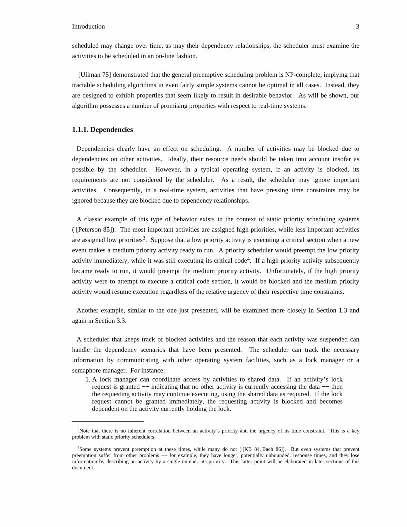
semaphore manager. For instance:1. A lock manager can coordinate access by activities to shared data. If an activity’s lock
request is granted −− indicating that no other activity is currently accessing the data −− thenthe requesting activity may continue executing, using the shared data as required. If the lockrequest cannot be granted immediately, the requesting activity is blocked and becomesdependent on the activity currently holding the lock.
3Note that there is no inherent correlation between an activity’s priority and the urgency of its time constraint. This is a keyproblem with static priority schedulers.
4Some systems prevent preemption at these times, while many do not ( [KB 84, Bach 86]). But even systems that preventpreemption suffer from other problems −− for example, they have longer, potentially unbounded, response times, and they loseinformation by describing an activity by a single number, its priority. This latter point will be elaborated in later sections of thisdocument.
4 Scheduling Dependent Real-Time Activities
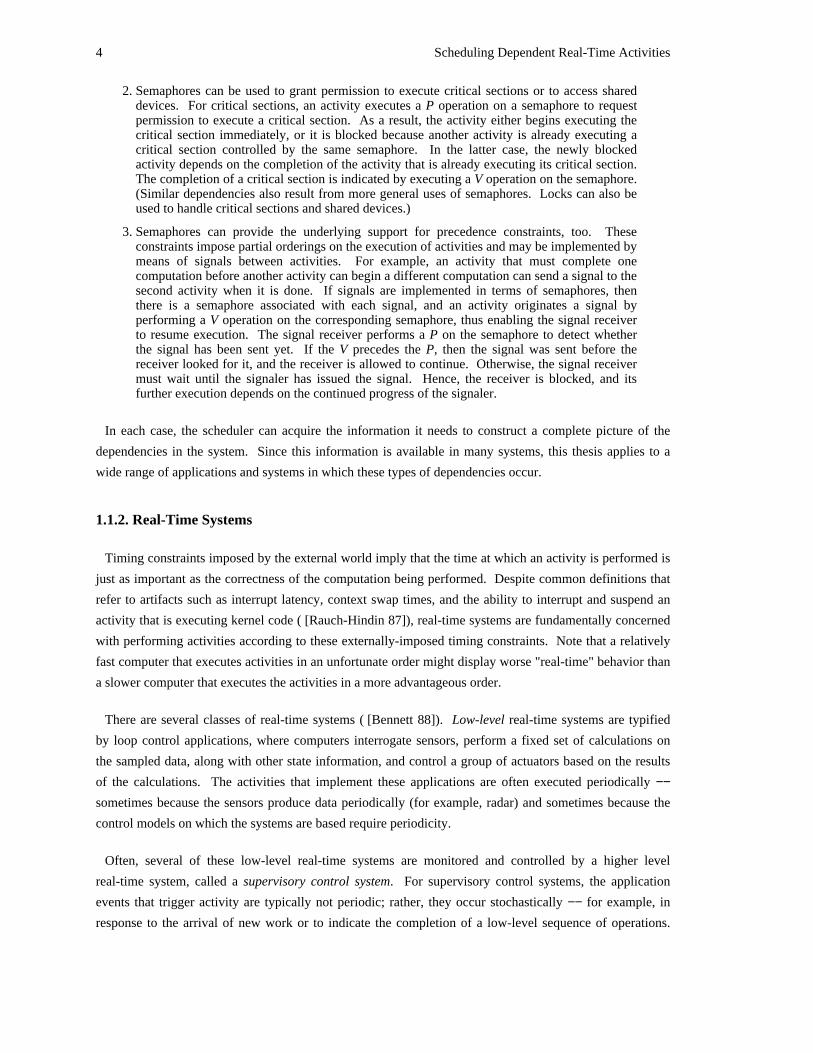
2. Semaphores can be used to grant permission to execute critical sections or to access shareddevices. For critical sections, an activity executes a P operation on a semaphore to requestpermission to execute a critical section. As a result, the activity either begins executing thecritical section immediately, or it is blocked because another activity is already executing acritical section controlled by the same semaphore. In the latter case, the newly blockedactivity depends on the completion of the activity that is already executing its critical section.The completion of a critical section is indicated by executing a V operation on the semaphore.(Similar dependencies also result from more general uses of semaphores. Locks can also beused to handle critical sections and shared devices.)
3. Semaphores can provide the underlying support for precedence constraints, too. Theseconstraints impose partial orderings on the execution of activities and may be implemented bymeans of signals between activities. For example, an activity that must complete onecomputation before another activity can begin a different computation can send a signal to thesecond activity when it is done. If signals are implemented in terms of semaphores, thenthere is a semaphore associated with each signal, and an activity originates a signal byperforming a V operation on the corresponding semaphore, thus enabling the signal receiverto resume execution. The signal receiver performs a P on the semaphore to detect whetherthe signal has been sent yet. If the V precedes the P, then the signal was sent before thereceiver looked for it, and the receiver is allowed to continue. Otherwise, the signal receivermust wait until the signaler has issued the signal. Hence, the receiver is blocked, and itsfurther execution depends on the continued progress of the signaler.
In each case, the scheduler can acquire the information it needs to construct a complete picture of the
dependencies in the system. Since this information is available in many systems, this thesis applies to a
wide range of applications and systems in which these types of dependencies occur.
1.1.2. Real-Time Systems
Timing constraints imposed by the external world imply that the time at which an activity is performed is
just as important as the correctness of the computation being performed. Despite common definitions that
refer to artifacts such as interrupt latency, context swap times, and the ability to interrupt and suspend an
activity that is executing kernel code ( [Rauch-Hindin 87]), real-time systems are fundamentally concerned
with performing activities according to these externally-imposed timing constraints. Note that a relatively
fast computer that executes activities in an unfortunate order might display worse "real-time" behavior than
a slower computer that executes the activities in a more advantageous order.
There are several classes of real-time systems ( [Bennett 88]). Low-level real-time systems are typified
by loop control applications, where computers interrogate sensors, perform a fixed set of calculations on
the sampled data, along with other state information, and control a group of actuators based on the results
of the calculations. The activities that implement these applications are often executed periodically −−sometimes because the sensors produce data periodically (for example, radar) and sometimes because the
control models on which the systems are based require periodicity.
Often, several of these low-level real-time systems are monitored and controlled by a higher level
real-time system, called a supervisory control system. For supervisory control systems, the application
events that trigger activity are typically not periodic; rather, they occur stochastically −− for example, in
response to the arrival of new work or to indicate the completion of a low-level sequence of operations.
Introduction 5
These events represent significant changes in the physical world and must be handled by the supervisory
control system in a timely manner. So, just like low-level real-time systems, supervisory control systems
have physically derived time constraints; and, in fact, meeting these time constraints is just as critical as it
is in low-level systems.
In addition to monitoring and directing the low-level real-time systems, supervisory control systems
perform strategic planning functions to coordinate the actions of the low-level systems in order to meet the
application’s objectives. The supervisory control systems, in turn, receive direction from higher level
management information systems (for example, to fill a given set of orders during the current shift in a
plant). Although supervisory control activities cooperate to provide their services, they still contend for
access to shared system and application resources.
Unfortunately, the policies that are prevalent in non-real-time systems to resolve such contention are
inappropriate, and may in fact be counterproductive, in real-time systems. For instance, in time-sharing
systems, fairness is desired and is obtained by, among other things, using FIFO queueing disciplines and
round-robin schedulers ( [Peterson 85]). This approach reflects the belief that all activities are equally
significant. However, in real-time systems this is clearly not the case −− some activities, and hence, some
time constraints, are decidedly more significant than others. In fact, while the failure to satisfy some timing
constraints may have no adverse effect on the physical process or platform being controlled, failing to
satisfy others can have catastrophic effects.
Throughput is another metric that is important in many non-real-time systems, but is not necessarily
meaningful in real-time systems ( [Jensen 76a]). In a real-time system, either all of the work that must be
done is actually performed or, if that is not possible, the most important application functions must be
performed. The latter case might not maximize throughput, but it does address the requirements of the
real-time system.
A few examples will illustrate the varying significance that may be attached to satisfying specific time
constraints.
First of all, consider a real-time supervisory control system in a process control setting −− a furnace and a
continuous caster in a steel mill. Molten steel of a specific chemistry is created from iron, scrap, and
additional materials in the furnace. When the metal in the furnace is ready to be converted into slabs of
solid steel, the molten metal is poured into a large ladle, transported to the caster, poured into the caster,
and cast into a long, continuous slab that is subsequently cut into individual slabs of appropriate length.
When the metal is originally poured into the caster’s "mold," it is liquid. It cools in the "mold" and is solid
when it emerges, ready to be cut. Several low-level real-time systems directly control the furnace, the
caster, and several related pieces of equipment. These systems are monitored, controlled and coordinated
by a supervisory control system.
In this setting, there are several types of supervisory control time constraints that can be examined.
Roughly speaking, they fall into three classes: (a) time constraints that, if missed, will result in potential
6 Scheduling Dependent Real-Time Activities
loss of life and property (for example, due to liquid steel spilling over the area); (b) time constraints
imposed by the physical world that have financial penalties if they are missed (for instance, losing quality
control statistics for products, resulting in potentially unsellable products); and (c) time constraints that are
not physically based and result only in inconvenience if they are missed (such as operator display requests).
Military systems also provide examples of the difference in importance between various time constraints.
For a fighter plane, for instance, the most importance activities are those that serve to keep the plane in the
air and the pilot alive; the activities that control weapons are less important, although, obviously, they are
still of great concern. On the other hand, aboard a ship, which will float stably without constant control, the
activities in charge of the defensive weapons systems may well be more important than those that steer the
ship.
The preceding examples demonstrate that there are a number of time constraints that characterize an
application and there are significant differences among the activities that must satisfy those time
constraints. It makes sense to talk about failing to satisfy time constraints in a dynamic system because
transient, and even permanent, increases in resource demands (relative to resource supplies) are possible.
Detecting these demand peaks and deciding which time constraints should be satisfied (and which should
not) are difficult tasks. In general, however, overall application performance and function should degrade
gracefully, maintaining the most critical functions for as long as possible.
Furthermore, although each activity operates under a time constraint, it is also classified according to its
relative importance (compared to other activities), and this importance is independent of the time
constraint. That is, there is no inherent correlation between the activity’s importance and its urgency −−which is captured by its time constraint. A critically important activity may require little computation time
and may have a very loose time constraint (relatively speaking). In that case, it is certainly not an urgent
activity, although it is an important activity. Conversely, a relatively unimportant activity may have a very
tight time constraint. Therefore, it is fairly urgent even though it is not very important in the global scheme
of things.
Many schedulers are able to deal with an activity’s importance (such as priority schedulers, as described
in [Peterson 85]) or its urgency (for example, deadline schedulers, as described in [Conway 67]), but few
attempt to distinguish between these two attributes or to use all of the information that is captured in both
of them.
One final difference between real-time systems and general-purpose computer systems should be noted.
In a real-time system, characteristics of the workload are often known very precisely. In a time-sharing
environment, on the other hand, the types of work being performed may vary greatly, and the operating
system may know little, if anything, about the processing and resource requirements of any given activity.
Specifically, in a real-time system, it is often possible to know (with some accuracy) how long an activity
must run to accomplish a goal. This type of information is available partly due to the historical
development of real-time systems: in order to construct reliable, real-time systems, designers used small
Introduction 7
routines that had predictable execution times. This allowed them to analyze system behavior to some
extent. As systems grew and become more sophisticated, it became more difficult to take this approach.
Nevertheless, it is still the approach that many system builders favor.
1.2. Schedulers and Scheduling Information
Two distinct approaches may be taken in designing and constructing a scheduler. On one hand, a
minimal scheduler can be provided. The scheduling may be list-driven, like the rate group schedulers used
by cyclic executives ( [GD 80, Stadick 83, MacLaren 80]); or it may employ a very simple algorithm, like a
priority scheduler. Such approaches impose a low system overhead. This may be entirely appropriate
when the goal is to maximize system throughput or to support a simple application structure so that
properties (such as worst case load behavior) can be demonstrated, but it is not obviously the best approach
for systems where the goal is to satisfy as many time constraints as possible or obtain the highest
application-specified value as possible. Furthermore, minimal schedulers may have limited applicability,
as evidenced by the fact that they are already stretched to the limit (or beyond) by today’s large, dynamic
real-time applications.
Alternatively, a complex scheduler may be used. In this case, application activities tell the scheduler their
individual needs and the scheduler attempts to satisfy them, making decisions based on global information
that the application does not possess. The more complete and accurate the information, the better the job5that the scheduler can do in managing resources ; and processor cycles, of course, are one particularly
important resource.
This thesis explores the latter philosophy by allowing the scheduler to use more information than usual in
order to do a better job of scheduling for supervisory control systems. There are two major points that must
be demonstrated to verify the quality of the scheduling:1. the individual scheduling decisions must be good (that is, the "right" activity must be selected
for execution);
2. the resources utilized to employ a more expensive scheduling algorithm must yield a benefitin terms of improved scheduling from the point of view of the application (that is, thescheduler must make better use of these resources than the application could).
Of course, not every application requires a complex scheduler, but some do, and this thesis explores the
use of complex schedulers to support those applications.
The previous discussion focused on time constraints without elaborating on the precise definition of these
constraints. The term has deliberately been used to capture the general notion that real-time computations
must satisfy certain timing requirements. We now introduce a formal method to describe time constraints
and introduce some additional terminology. Each activity in a real-time application is composed of a
5Improved scheduling can also be obtained by devoting more resources to analyzing a fixed amount of scheduling information.Although the main thrust of this thesis is to study the use of more information than usual, the algorithm to be studied also requiressignificant resources for the scheduler. The resulting implications will be discussed later in the document.
8 Scheduling Dependent Real-Time Activities
sequence of disjoint computational phases, also known simply as phases. The application as a whole
makes progress when its component activities make progress; and each activity makes progress by
completing its computational phases. Therefore, the completion of a computational phase marks
measurable progress for the application, and this progress is expressed in terms of value units. Associated
with each phase, then, is a time-value function ( [Jensen 75]) that specifies that phase’s time constraint −− it
indicates the value acquired by the application for completing the phase as a function of time.
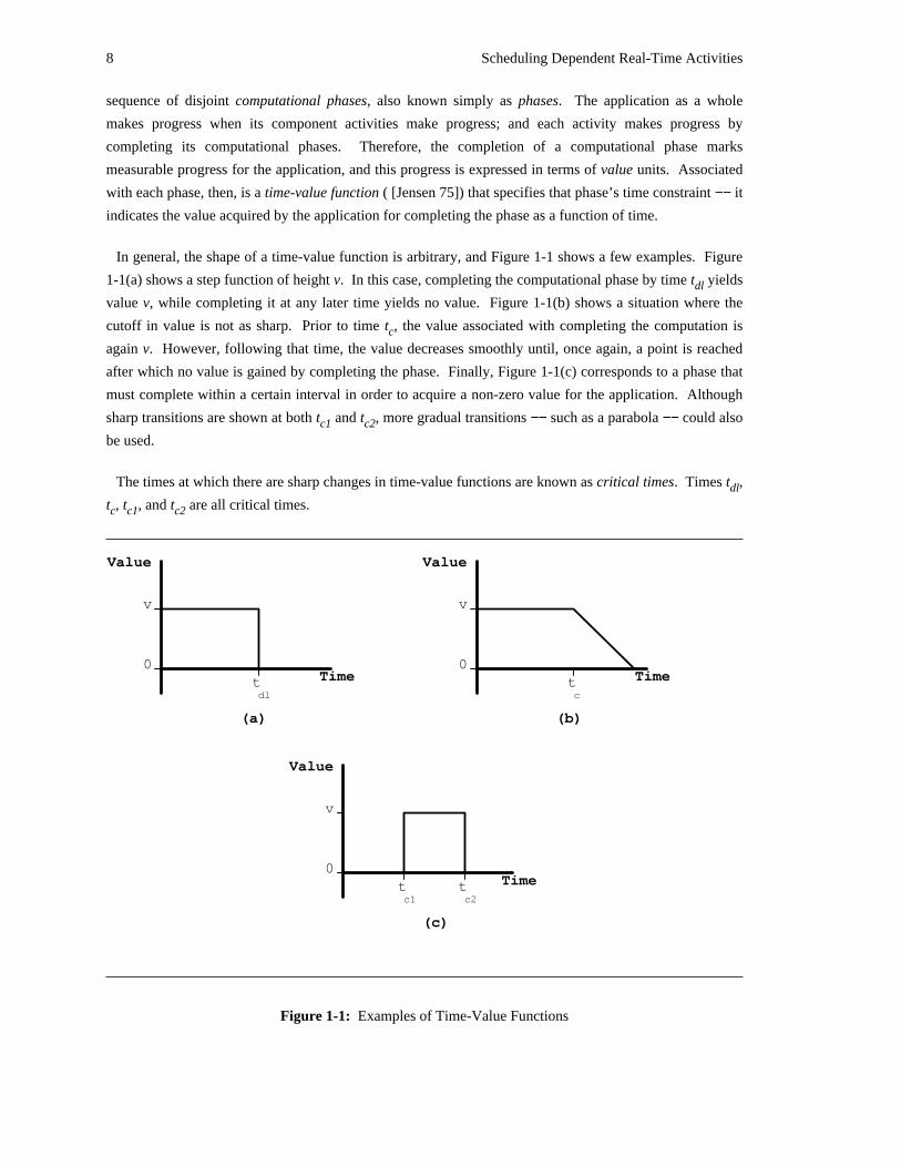
In general, the shape of a time-value function is arbitrary, and Figure 1-1 shows a few examples. Figure
1-1(a) shows a step function of height v. In this case, completing the computational phase by time t yieldsdl
value v, while completing it at any later time yields no value. Figure 1-1(b) shows a situation where the
cutoff in value is not as sharp. Prior to time t , the value associated with completing the computation isc
again v. However, following that time, the value decreases smoothly until, once again, a point is reached
after which no value is gained by completing the phase. Finally, Figure 1-1(c) corresponds to a phase that
must complete within a certain interval in order to acquire a non-zero value for the application. Although
sharp transitions are shown at both t and t , more gradual transitions −− such as a parabola −− could alsoc1 c2
be used.
The times at which there are sharp changes in time-value functions are known as critical times. Times t ,dl
t , t , and t are all critical times.c c1 c2
tt
(c)
(b)(a)
Value
Time0
t
v
v
0Time
Value
Value
Time0
tdl
v
c2c1
c
Figure 1-1: Examples of Time-Value Functions
Introduction 9
The step function shown in Figure 1-1(a) illustrates several key ideas and allows the introduction of some
important terminology. First of all, time t is referred to as a deadline since it represents the last instant atdl
which the phase can complete and still make a meaningful contribution to the accrued value for the
application. Value v is called the importance of the phase. If every time-value function were a step-
function and all of the step functions had the same height (importance), then each phase that was completed
would make an identical contribution to the progress of the application and an appropriate scheduling
strategy would complete as many phases as possible prior to their respective deadlines. If, however,
different phases were to have different importances, then they would make different contributions to the
value accrued by the application and the scheduling strategy that would maximize that value would be
different. Considered over the lifetime of an application, a greater accrued value represents a more
successful application.
If resource demands, including those for processor cycles, are sufficiently low, then all activities can be
scheduled, thereby accruing a large value for the application. However, in the event that it is impossible to6satisfy all of the activities’ resource demands, an overload exists . In this case, some subset of the
activities will meet their time constraints, while others will not, resulting in a lower accrued value for the
application. Under overload, the scheduler should maximize the value accrued by the application.
With an understanding of the simple step time-value function and the vocabulary introduced above,
consider again the notion that a scheduler can do a more effective job when it has more complete or better
quality information on which to base decisions. Given specific types of information, consider the
algorithms a scheduler can employ (unless otherwise noted, these are all discussed in [Conway 67], [Janson
85] or [Peterson 85]):
• no information −− there is no way to distinguish activities so round-robin or randomscheduling of ready activities would be appropriate;
• relative importance of activities −− priority scheduling of ready activities; this algorithm wouldalways run the highest priority (most important) ready activity;
• deadline and required computation time of activities −− deadline scheduling, where the readyactivity with the nearest deadline is always selected to run, or slack-time scheduling, where the
7ready activity that has the least slack-time is always selected to run, would be optimalalgorithms with this information;
• time-value functions ( [Jensen 75]), which capture importance and timing requirements −−more complex schemes such as best-effort scheduling ( [Locke 86]) of ready activities can beemployed; Locke showed that under his model, this approach can be more effective than thoselisted above.
This thesis explores the consequences of allowing the scheduler to have access to not only the activities’
time-value functions and their required computation times, but also to information describing the
6Overloads are not uncommon in operational supervisory control systems. In fact, in dynamic environments, it is impractical, if notimpossible, to eliminate overloads by means of system or application design methods. This is because the approaches that mayeliminate overloads in small, static systems, which typically depend on the predictable nature of the environment or the allocation ofsufficient assets (processors, memory, devices, and so on) so that peak demand can be handled, do not scale well to large, dynamicsystems.
7slack-time = deadline - present time - required computation time.
10 Scheduling Dependent Real-Time Activities
dependency relationships existing between activities. This enables the system to take into account the time
constraints of blocked activities, allowing a better ordering of activities, along with earlier detection and
better resolution of overloads.
Notice that the dependency information that is to be used by the proposed scheduling algorithm is not
very exotic or difficult to obtain in many cases. Often, the operating system or a system utility, such as a
lock manager, holds key pieces of this information. Whenever an activity is unable to gain immediate
access to a shared resource, it is typically blocked. At that point, the system is capable of noting which
resource is being accessed, as well as the identities of the activities holding and requesting the resource. In
other cases, straightforward extensions to the operating system interface would provide the necessary
dependency information for the scheduler’s use. As a result, if the algorithm can be demonstrated to have
sufficient merit, an implementation would not seem to be unduly difficult.
1.3. Scheduling Example
In order to demonstrate some of the points that have been made earlier and to illustrate the type of
problem addressed by this thesis, consider an example.
Assume that there are only three activities, each consisting of only a single phase. Designate these phases
p , p , and p . Phase p has a relatively low importance, requires four time units of execution time toa b c a
complete, and must complete execution within 15 time units of its initiation. It requires the use of shared
resource r. It requests access to r after it has executed for one time unit, and releases r after it has executed
for a total of three time units.
Phase p has a medium importance, requires three time units of execution time, and must complete withinb
four time units of its initiation. It also uses shared resource r. Like p , it requests r after it has executed fora
one time unit and releases it after it has executed for a total of three time units.
Phase p has a relatively high importance, requires four time units to complete execution, and mustc
complete within ten time units of its initiation. It does not access shared resource r.
All of these phases are initiated as a result of external events. Suppose that the event that initiates phase
p occurs at time t = 0, and the event that initiates both p and p occurs two time units later. This impliesa b c
that the deadline for completing phase p is time t = 15, the deadline for completing phase p is at time t =a b
6, and the deadline for completing phase p is time t = 12.c
If these phases are to be scheduled using a priority scheduler, then it seems clear that their importance to
the application should act as an indication of their priority. Therefore, if Pri() is a function that returns the
priority of a phase:
Pri(p ) < Pri(p ) < Pri(p )a b c
Also notice that this is a situation where urgency, when defined as the nearness of a deadline, is not the
same as importance. To see this, let DL() represent a function that returns the deadline of a phase. Then:
DL(p ) < DL(p ) < DL(p )b c a
Introduction 11
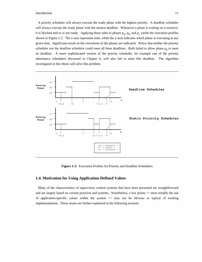
A priority scheduler will always execute the ready phase with the highest priority. A deadline scheduler
will always execute the ready phase with the nearest deadline. Whenever a phase is waiting on a resource,
it is blocked and so is not ready. Applying these rules to phases p , p , and p yields the execution profilesa b c
shown in Figure 1-2. The x-axis represents time, while the y-axis indicates which phase is executing at any
given time. Significant events in the executions of the phases are indicated. Notice that neither the priority
scheduler nor the deadline scheduler could meet all three deadlines. Both failed to allow phase p to meetb
its deadline. A more sophisticated version of the priority scheduler, for example one of the priority
inheritance schedulers discussed in Chapter 6, will also fail to meet this deadline. The algorithm
investigated in this thesis will solve this problem.
rl = release rg = grant rrq = request r
rl
rl
rl,g
rl,g
rq
rq
rq,g
rq,g
t
pa
pb
pc
pc
pb
pa
5 100
0 105t
Deadline Scheduler
Static Priority Scheduler
RunningPhase
PhaseRunning
Figure 1-2: Execution Profiles for Priority and Deadline Schedulers
1.4. Motivation for Using Application-Defined Values
Many of the characteristics of supervisory control systems that have been presented are straightforward
and are largely based on current practices and systems. Nonetheless, a few points −− most notably the use
of application-specific values within the system −− may not be obvious or typical of existing
implementations. These issues are further explained in the following sections.
12 Scheduling Dependent Real-Time Activities
1.4.1. Accrued Value
Evaluating a scheduling algorithm by determining the total value it accrues on behalf of an application is
unusual. However, not only is it intuitively appealing, it is also appropriate in many cases.
The intuitive appeal lies in the view that accumulating value represents making progress. As each
activity completes designated portions of its execution, value accrues to indicate the utility of that particular8computation to the application .
Similarly, the idea of minimizing a cost function is often found in deterministic scheduling problems in
operations research. Some of this work is summarized in [DLRK 81].
While this might sound plausible as a metric, there remains the question of whether values can be
assigned meaningfully to computational phases of an activity. In many instances, there is strong reason to
believe that this is the case.
The class of process control applications provides one example of the applicability of this approach.
Typically, one or more processes are being controlled or one or more products are being manufactured
under the supervision of a single supervisory control computer system. Since the goods being produced
have a monetary value, it is possible to assign values to particular activities based on the commercial worth
of the goods being produced by each activity. Consequently, the use of a scheduler that maximizes the
amount of value accrued for the application is actually maximizing the commercial value of the goods
being produced. This seems entirely reasonable. (Conversely, if it seemed more natural, the notion of
monetary loss or penalty could be used instead of the monetary value or profit outlined. The underlying9notion is essentially the same in either case.)
During an overload, when there are insufficient resources to meet the overall demand, some activities
may not be scheduled. In fact, it would be possible that during an overload involving three or more
activities, the activity with the highest individual value would not be scheduled. Rather, two or more
activities with lower individual values, but with a higher combined value, could be scheduled.
This overload behavior should be contrasted with that of other scheduling policies. For instance, a
8Notice that summing individual values is only one possible way to accrue value for an application. More complex accrual rulesmay also be worthy of investigation. For example, it may be necessary to complete a sequence of time-constrained computations inorder to accomplish a meaningful goal for the application, in which case, perhaps no value should be accrued for any computationsuntil the last one has successfully completed. Or the effect of completing two time-constrained computations is greater than the sumof their individual values, indicating that their values could be combined in another way. As always, the goal is to perform theapplication as well as possible; and future experience will contribute to a better understanding of how to express an application’s goalsin terms of values and value accrual rules that best meet its requirements.
9The use of monetary measures to determine schedules has long been used in the field of operations research for job shopscheduling. The model used in this work differs somewhat from that model. This is dealt with in some depth in Chapter 6. Briefly,the typical job shop model assumes that the set of orders currently known will all be filled at some point in time. That is, all activitieswill eventually be run. However, in real-time computer systems, some activities are of only transient value because they are runfrequently or because they must be run in a timely fashion or not at all due to the quality of the information or the physical timeconstraints of the application. Therefore, not all activities will necessarily be run.
Introduction 13
priority scheduler would always execute the activity with the highest individual value at any given time
(assuming that the priorities assigned to activities corresponded to the commercial worth of the activity as
described previously). In the case just outlined, this would result in a lower total value than the method that
maximized value.
A steel mill application can illustrate this point, while demonstrating the dynamic nature of the
assignment of values to tasks. The steel mill under consideration has a furnace and caster that combine to
transform raw materials into slabs of finished steel of specified chemistry. There are two functions that are
particularly interesting: chemistry control, which controls the chemical composition of the steel being
produced, and quality control tracking, which follows the progress of the steel through various stations in
the mill including the caster and associates a specific chemistry with each foot of every steel slab produced
by the mill. A single supervisory control computer monitors and controls both of these functions.
During overloads, the supervisory computer may have to decide which function should be run. Most
often, the value associated with the quality control activity should be higher than that associated with the
chemistry control activity. This is because it is important to know what is in each steel slab that is sold. In
fact, since many customers will not buy a slab without detailed knowledge of its chemistry, the profit that
would be realized from the slab is at stake if the tracking activity does not execute in time. On the other
hand, if the chemistry control activity is not executed, the chemistry of the steel may be different from what
was intended. This is acceptable if the resultant chemistry is one that can be sold or can be further
processed to obtain such a chemistry. Notice that the chemistry −− even if it is not the chemistry that was
originally intended −− is known and can be tracked by the quality control activity.
The dynamic nature of value assignments is shown by the fact that the above generalization does not hold
in every case. When a particularly rare chemistry is desired, it is sometimes the case that the steel cannot
be sold if the chemistry is not exactly right, therefore placing the profit for the heat in jeopardy if the
chemistry control activity is not run. It is possible that the profit involved, especially for a specialty steel,
will outweigh the profit that will result from tracking steel slabs of more typical chemistries through the
rest of the mill. Since these decisions vary with each heat (mix) of steel, values must be assigned to the
chemistry control and quality control tracking activities dynamically to correspond to each heat.
Military defense systems are a second class of applications that seem to allow values to be assigned to
component activities meaningfully and would benefit by using a scheduler that maximized accrued value
for the application. In this case, the value accrued for an activity controlling a defense system would be
derived from the number of lives or the number of other military assets that can be saved. As unsettling as
it is to consider, it seems wise to employ a scheduler that maximizes the number of lives or assets that are
successfully defended.
These examples make use of the fact that there is a common "currency" in which values can be expressed
naturally −− money in process control situations and lives or other military assets in combat systems. In
14 Scheduling Dependent Real-Time Activities
10such situations, it is relatively straightforward to assign values to various activities . Other applications
may require that values take into account a number of different factors −− money, lives, operator
satisfaction, and so forth −− and appropriate weightings of these factors will have to be developed to
produce acceptable and meaningful activity values.
Of course, the real test of the utility of this approach will come in the future when scheduling algorithms
that maximize application-defined value are employed in production systems −− or, perhaps, prototype
versions of production systems. At that time, the performance of these systems can be compared directly to
alternative approaches. In order to prepare for such tests, the notion of maximizing the accrued value for
an application must be further explored. This thesis makes another contribution to that effort.
1.4.2. Time-Value Functions
As shown in the above discussion, the notion of assigning values to application activities and scheduling
activities to maximize the accrued value for the entire application has merit in a wide range of applications.
These assigned values reflect the relative importances of the activities that they represent.
Since the systems under consideration for this work are real-time systems, the value associated with the
completion of a computation varies as a function of time. For example, in an automated assembly
application, the value of closing a mechanical manipulator to grasp a part on an assembly line is a function
of time. If the grasping motion is completed too soon, the part will not have reached the manipulator yet.
If the grasping motion is completed too late, the part will have already passed by the manipulator.
Time-value functions facilitate the description of the time constraints and relative importances of the
activities comprising a real-time application. The time-value function records the value to be accrued by
completing the designated computational phase at each point in time.
Time-value functions seem to be a fairly natural expression of the utility of completing a given
computation as a function of time in many situations. A skilled operator in a process control environment
or a carefully constructed functional requirements document for the system will often be capable of
describing all of the information encoded in a time-value function.
Although time-value functions are a relatively new formalism for expressing the relative urgency and
importance of each activity in a real-time system, they are beginning to make the transition into practice
and have been used successfully in a few selected contexts ( [CMUGD 90, Alpha 90]).
10This act of assigning values to specific activities comprising an application corresponds roughly to the normal assignment ofpriorities to activities (where the activities are often called processes or tasks). Through many years of experience, this procedure isunderstood to some extent, but there are still some difficulties. For instance, in many modern applications a number of activitiescoordinate to provide a single application-level logical function, such as material tracking −− that is, keeping track of material as itmoves through a plant. In such systems, one activity provides a specific service, access to the tracking database, to a number of otheractivities that have widely varying values. The assignment of a single value to the server activity is problematic. If it has beenassigned a lower value than the activity that it is currently serving, then it may not be scheduled as quickly as it should be. On theother hand, if it has been assigned a higher value than the activity it is serving, then it may consume resources that could, and should,be used by other activities. This problem is alleviated if an approach is taken where the activities in the computer application cancorrespond directly to the application-level logical functions, while still providing for modular construction of the application. Thishas been done in the Alpha Operating System ( [Alpha 88]).
Introduction 15
1.5. Technical Approach
The technical approach described in this section was adopted to address the problem of scheduling with
dependencies and to explore and evaluate potential solutions. Briefly, the approach consists of the
following major steps:1. define a computational model within which to work;
2. devise an algorithm that possesses the required properties and express it within thecomputational model;
3. insofar as possible, demonstrate analytically the correctness, utility, and tractability of thealgorithm;
4. simulate the performance of the algorithm on common classes of supervisory control systemsand compare with other relevant algorithms or ideals.
The following sections outline each of these steps, and the results generated by this approach constitute
the majority of this thesis.
1.5.1. Define Model
The first step, defining a computational model, is intended to provide a clear, useful framework that will
capture the essential aspects of the problem to be solved and will also support the specification of
unambiguous solutions, embodied primarily as scheduling algorithms. The need for a model that exhibits
all of the desired problem features, while excluding all factors that are non-essential for the problem
statement and solution is obvious. If the work is done with the simplest model that accurately expresses the
problem, then the work will be more comprehensible and succinct. Equally important is the requirement
that the model support the unambiguous specification of scheduling algorithms. Without such definitions,
the ability to perform precise/definitive analytic proofs to demonstrate properties of an algorithm will be
lost. Also, a set of requirements for problem solutions is formulated in terms of the computational model.
1.5.2. Devise Algorithms
After the model has been created, it is possible to begin exploring various algorithms within the
framework provided by the model. While the computational model is intended to support the development
of a number of scheduling algorithms and will provide an excellent platform for the extension of this work
in the future, this thesis does not explore a wide range of alternative algorithms exhaustively. Rather, it
identifies and characterizes the behavior and performance of a single algorithm that has the desired
properties, called the Dependent Activity Scheduling Algorithm (DASA). This algorithm will be described
in two forms −− a formal, mathematical form that will be used to define the algorithm and to support
analytic proofs and a procedural form to provide a measure of the algorithm’s complexity and to support11the simulation work that has been done.
11Actually, the mathematical definition features non-determinism in certain places, indicating that ordering is unimportant withrespect to the algorithm at those points. The procedural definition, however, does not contain any non-determinism and so can beviewed as a single specific implementation of the algorithm that the mathematical definition describes.
16 Scheduling Dependent Real-Time Activities
1.5.3. Prove Properties Analytically
Once the DASA algorithm has been defined, analytic proofs that demonstrate that it satisfies the problem
requirements may be devised. The formal model that is used to describe the scheduling algorithms is based
on automata that accept certain sequences of scheduling events. There is a different automaton associated
with each distinct scheduling algorithm. So, for example, the automaton associated with the DASA
algorithm will accept any sequence of scheduling events that is consistent with the behavior of the DASA
algorithm. Such automata can also accumulate the value assigned to an execution history. By comparing
the execution histories accepted by the automata corresponding to different scheduling algorithms, proofs
can be constructed that show that two scheduling algorithms accept different histories. Furthermore, the
proofs may compare the values accumulated for all of the execution histories accepted by the automata
representing certain scheduling algorithms for a specific set of phases with specific time-value functions
and computation time requirements. (Taken together, these last two items −− a phase’s time-value function
and its computation time requirement −− are referred to as the phase’s scheduling parameters.) Such
comparisons can be used to demonstrate that one scheduling algorithm is capable of generating schedules
that are superior to those of another algorithm, measured in terms of total value accrued by the application
during its execution history.
Unfortunately, real-time systems featuring complex, dynamic dependency relationships are quite
complex. And, although the analytic proofs can make some observations about the correctness, behavior,
and value of the algorithm, a complete case for its utility cannot be made without demonstrating its
performance under realistic conditions. To address this need, simulations have been carried out to
investigate the performance of the DASA algorithm and to demonstrate properties that cannot be proven
analytically.
1.5.4. Simulate Algorithm
A parameterized workload has been devised that can mimic various numbers of activities displaying a
range of access patterns to a set of shared resources. Using this workload, a suite of simulations has been
run. These simulations compare the benefit of using the DASA algorithm instead of a more standard
algorithm −− for instance, a static priority or deadline scheduling algorithm with FIFO queueing for access
to each shared resource. They also compare DASA’s performance with a reasonable estimate of the
theoretical maximum value that can be obtained. The DASA scheduling algorithm is relatively complex
when compared to more standard scheduling algorithms. Consequently, in a uniprocessor implementation
of the algorithm, DASA will require more time to select an activity to execute than a more standard
algorithm would. In order to be fair in performing comparisons among scheduling algorithms, this
additional overhead is also taken into account. The simulation results reveal situations in which applying
the DASA algorithm will probably be profitable.
Chapter 2
The Scheduling Model
Models are central to abstract study. They allow the salient features of a potentially complex system to
be isolated and restrict the size of the space of possibilities to be investigated. Properly specified, a model
provides an unambiguous definition of the behavior of a system and highlights the underlying assumptions
that are made by the investigator. Within the framework of the model, simulations and analytic analyses
may be performed.
To take advantage of all of these properties, a model has been devised that possesses the necessary
richness and within which scheduling algorithms can be studied. This chapter presents this model and
describes the rationale that shaped it.
A formal computational model has been constructed to facilitate the definition and formal analysis of
scheduling algorithms. Initially, this model is presented informally in order to allow for a natural
discussion of the issues that shape the model and the intended structure of the model and the environment
provided by real-time applications. This is followed with a formal description that provides a detailed,
precise specification of the model.
2.1. Informal Model and Rationale
The informal discussion of the computational model will describe each of the principal elements of the
model in general terms. This should allow the reader to have an intuitive grasp of the interplay of various
elements of the model without having to wade through a mass of symbols and mathematics. This will set
the stage for the presentation of the formal model, where all of the details will be specified for each of the
principal elements of the model.
2.1.1. Applications, Activities, and Phases
As mentioned in the previous chapter (in Sections 1.1 and 1.2), an application is composed of a set of
activities. Each activity, in turn, comprises a sequence of computational phases, and each computational
phase is characterized by a required computation time (indicating the amount of processor time it needs to
complete execution, assuming that all of the shared resources it needs are immediately available) and by a
time-value function that indicates its importance and urgency. At any given time, an activity is operating in
a single computational phase so that the activity can be uniquely identified by designating the phase that is
17
18 Scheduling Dependent Real-Time Activities
currently underway. Therefore, the complete set of activities can always be represented by the set of12phases currently in progress , and this set can be designated as:
{p , p , p , . . . }0 1 2
The execution of an application involves sharing the single processor among the set of active phases over
time. The determination of which phase to run at any given time is made by the scheduler, one of the major
components of the operating system, based on the relevant information available to it.
2.1.2. Shared Resources
Phases may access shared resources. A request for such access is signaled by a phase by means of a
‘request’ event for the specific resource desired. Permission to access a shared resource is given to the
phase by means of a ‘grant’ event.
Locks and semaphores, for example, arbitrate access to shared resources in a real system. As was stated
in Chapter 1, signals that synchronize the execution of activities can also be implemented based on
semaphores.
This research assumes that the shared resources required by a phase to complete successfully are not
known at the start of the phase. Although the resource requirements may be known for some phases in
specific applications, they may not be known for all phases in all applications. Therefore, the decision has
been made not to rely on the availability of this information. (If some resource requirements are known,
the resources can be requested immediately after the phase has started so that the scheduler can make
decisions based on as much information as possible.)
There are often good reasons why not all of the shared resources that will be needed by a phase are
known when the phase is initiated. For example, concurrency may be increased by performing some
computation before requesting a shared resource. Concurrency can be increased due to two factors: (1) if
the request is made later, then the intervening time is available for other phases to access the shared
resource, and (2) finer granularity accesses are possible, allowing more of the data to remain available for
other phases.
An example of this second point is found in accessing a tracking database. Assume that at the start of a
phase, it is known that a tracking database record will be updated, but that the exact identity of the record to
be accessed is not known. It is determined by correlating various data sources as part of the phase. This
leaves the phase two options: either it can request access to the entire database (or a possibly significant
subset of it) at the start of the phase, thus denying other phases access to the database; or it can wait until it
has determined the record to be accessed and then request access to only that record, thus allowing other
phases nearly unrestricted access to the entire database for the phase’s duration.
12For the purposes of this model, a phase is considered to be "in progress" as soon as it is made known to the operating system. So,for instance, a phase that has never executed a single instruction of its code is nonetheless considered to be in progress −− it hasprogressed far enough to submit its initial resource request (in terms of required processing time, importance, and urgency) to thesystem.
The Scheduling Model 19
All shared resources that are held by an activity must be released at the completion or abortion of each
computational phase. Although this assumption may seem to be restrictive, it is justifiable on two counts.
First of all, when a phase represents a distinct logical stage in a computation, there is good reason for
expecting that the resources used to carry out that phase may be released upon its completion. Of course, if
phases are used to represent very fine grained portions of a computation, then this assumption may be
called into question. However, since each phase is a unit of computation that corresponds to a single
time-value function, and since the time constraints that dictate the time-value functions are derived by the
physical necessity of completing a computation in a certain time frame, it seems clear that using phases to
delimit very small portions of an activity departs from the expected, and useful, application of phases to
decompose activities in a real-time system.
The existence of stylized applications or system facilities gives rise to the second justification for the
assumption that all shared resources are released at the completion of a computational phase. For instance,
an atomic transaction facility would exhibit exactly this behavior with respect to shared resources. Yet,
while the use of transactions in real-time systems is appealing, the question of how to schedule them is
unsolved. By allowing this model to capture the behavior of transaction facilities as well as the assumed
normal behavior of real-time activities, the work presented here may constitute a somewhat greater research
contribution.
2.1.3. Phase Preemption
At any given time there is one phase that is actively executing on the processor. That phase may be
preempted by the scheduler at any time. A preemption is signaled by a ‘preempt-phase’ event. Should the
scheduler subsequently determine that the phase should be resumed, it would issue a ‘resume-phase’ event.
2.1.4. Phase Abortion
The scheduler may decide to abort a computational phase at any time. The scheduler initiates an abort by
issuing an ‘abort-phase’ event for the chosen phase.
A phase might be aborted to free a shared resource more quickly than it would otherwise be freed. Or, a
transaction facility ( [Eswaran 76]) might issue an abort in response to a component failure or to resolve a13detected deadlock .
The amount of time required to completely process an abort depends on the number and type of resources
held by the phase being aborted. Each time access to a new shared resource is granted to a phase, the
amount of time required to abort the phase is incremented by an amount dependent on the newly granted
resource.
13A deadlock exists among a set of phases if each member of the set requires access to a resource that is held by some other memberof the set in order to make further progress. In such a situation, none of these phases can make progress, and an abort may be issued toforce one phase to release the resource(s) it is holding, thereby resolving the deadlock.
20 Scheduling Dependent Real-Time Activities
The incremental amount of abort time associated with a resource may arise from several sources. For
instance, for resources that are treated like data objects in a traditional database system, each data object
altered during the course of an aborted transaction must be returned to the same state it had prior to the
transaction. The time required to restore this pre-transaction state is determined by the time required to
find the desired value followed by the time required to actually update the data object.
In other cases, more must be done than merely restoring the state of the appropriate memory locations.
Real-time systems often control physical processes by regulating actuators that cause changes in the
physical environment. Permission to manipulate an actuator may be acquired by successfully requesting
exclusive access to a shared resource that is logically associated with the actuator. Once access to the
resource has been granted, the actuator is available to, and manipulated by, the requesting computational
phase. If the phase is subsequently aborted during its execution, then it is quite possible that the actuator
may have to be manipulated once more in order to return the physical environment to an acceptable state.
The amount of time required for such compensating actions must be included in the time allotted for abort
processing for each resource of this type.
Those shared resources that represent synchronization signals between computational phases carry with
them an infinite abort time. This reflects the fact that aborting a phase that would generate a signal upon its
successful completion should not cause that signal to be sent. Rather, the signal’s receiver must wait until
the signaler has truly completed execution.
Following the completion of an abort, the affected activity will be ready to reexecute the aborted phase if
time and resources permit.
2.1.5. Events
To motivate the development of a formal model, imagine that all of the major components of an operating
system interact by signaling specific events to one another. Conceptually, these events encapsulate
information and commands, and they can originate within the operating system or from the computational
phases comprising the application.
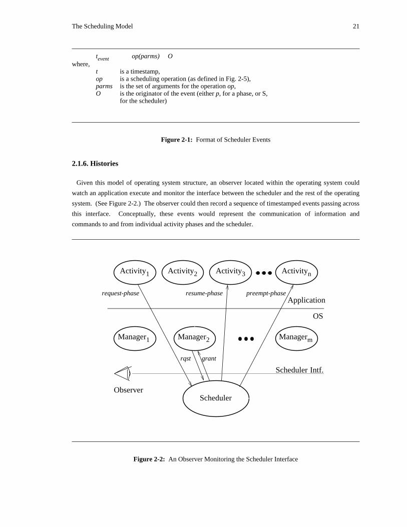
As shown in Figure 2-1, each event includes an event timestamp, an operation name, appropriate
arguments for the operation, and the originator of the event. Timestamps are used to provide a global
ordering of all scheduling events. There are a small number of scheduler-related operations, which will be
described below. And, as far as scheduling-related events are concerned, the originator of an event is either
the scheduler itself (meaning that the event passed across the interface from the scheduler to the rest of the
operating system, possibly continuing on to an application phase) or an individual phase (meaning that the
event passed from that phase to the scheduler, via the operating system).
The Scheduling Model 21
t op(parms) Oeventwhere,
t is a timestamp,op is a scheduling operation (as defined in Fig. 2-5),parms is the set of arguments for the operation op,O is the originator of the event (either p, for a phase, or S,
for the scheduler)
Figure 2-1: Format of Scheduler Events
2.1.6. Histories
Given this model of operating system structure, an observer located within the operating system could
watch an application execute and monitor the interface between the scheduler and the rest of the operating
system. (See Figure 2-2.) The observer could then record a sequence of timestamped events passing across
this interface. Conceptually, these events would represent the communication of information and
commands to and from individual activity phases and the scheduler.
Application
OS
Scheduler
Activity1 Activity2 Activity3 Activityn
request-phase preempt-phaseresume-phase
Observer
Scheduler Intf.
Manager2Manager1 Managerm
grantrqst
Figure 2-2: An Observer Monitoring the Scheduler Interface
22 Scheduling Dependent Real-Time Activities
Such a sequence of scheduling events is called a history. In general, any sequence of scheduling events
constitutes a history, although not all histories are meaningful. To aid in recognizing which histories are
potentially meaningful, definitions have been developed for well-formed histories (for example, timestamps
must increase throughout the history and only the event operations listed in Figure 2-5 can be included in
it) and for legal histories −− that is, well-formed histories where the sequence of events is plausible, for
example, ‘request’s precede ‘grant’s. Operations on histories have also been defined to facilitate their
manipulation. For simplicity, the only histories that are ever dealt with in formal analysis, after the
introduction of these definitions, are legal, well-formed histories. (The definitions referred to in this
paragraph are presented in Section 2.3.2.8.)
Different schedulers will select different activities for execution based on the relevant scheduling
parameters for each phase under consideration. Consequently, different histories will be generated by
different schedulers, even though they may be executing the same application under the same conditions.
Examining these histories allows the performance and behavior of the schedulers to be compared and
contrasted. Formally, the histories are examined by a special type of finite state automaton, called a
scheduling automaton.
2.1.7. Scheduling Automata
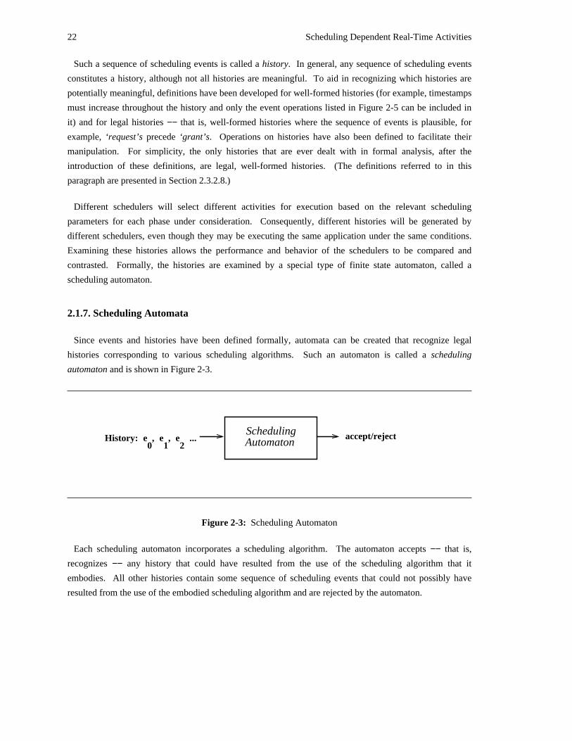
Since events and histories have been defined formally, automata can be created that recognize legal
histories corresponding to various scheduling algorithms. Such an automaton is called a scheduling
automaton and is shown in Figure 2-3.
SchedulingHistory: e
0, e
1, e
2 ... accept/reject
Automaton
Figure 2-3: Scheduling Automaton
Each scheduling automaton incorporates a scheduling algorithm. The automaton accepts −− that is,
recognizes −− any history that could have resulted from the use of the scheduling algorithm that it
embodies. All other histories contain some sequence of scheduling events that could not possibly have
resulted from the use of the embodied scheduling algorithm and are rejected by the automaton.
The Scheduling Model 23
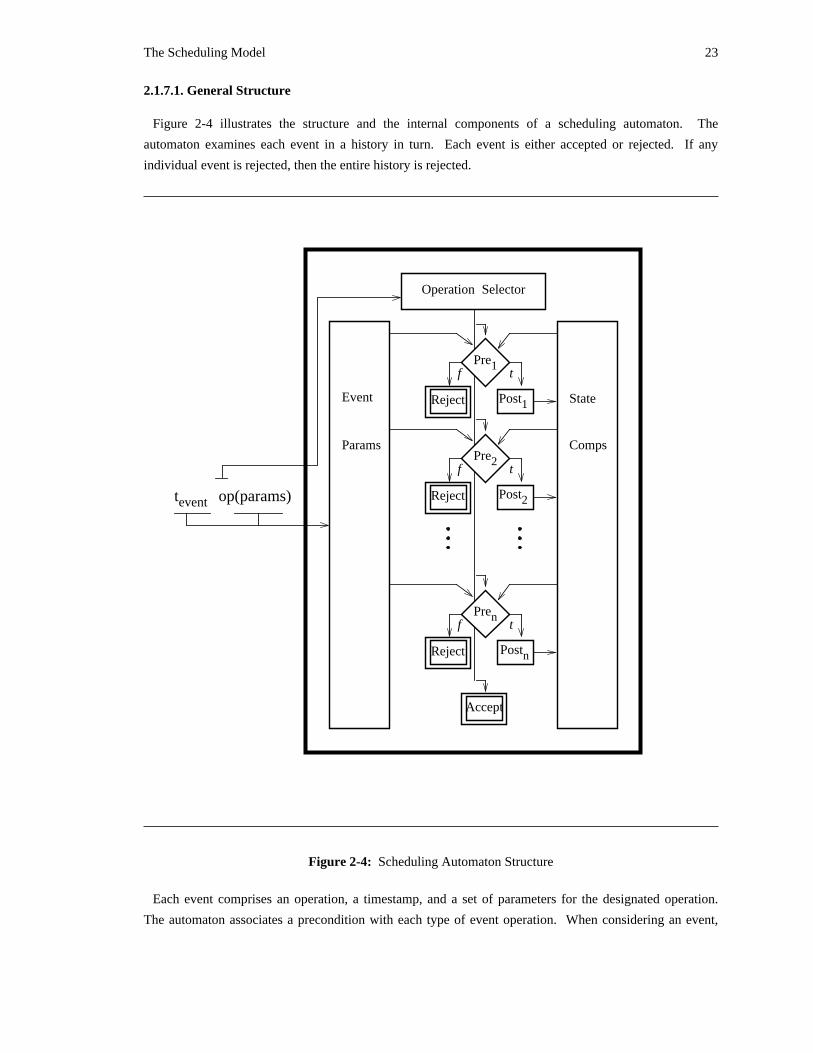
2.1.7.1. General Structure
Figure 2-4 illustrates the structure and the internal components of a scheduling automaton. The
automaton examines each event in a history in turn. Each event is either accepted or rejected. If any
individual event is rejected, then the entire history is rejected.
Pre1
Reject Post1
Operation Selector
State
Comps
Event
Params
tf
Pre2
Reject Post2
tf
Pren
Reject Postn
tf
Accept
tevent op(params)
Figure 2-4: Scheduling Automaton Structure
Each event comprises an operation, a timestamp, and a set of parameters for the designated operation.
The automaton associates a precondition with each type of event operation. When considering an event,
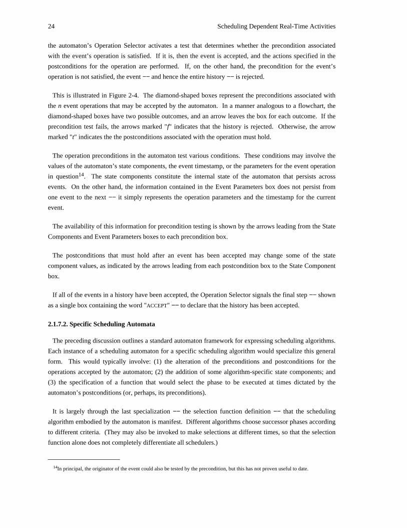
24 Scheduling Dependent Real-Time Activities
the automaton’s Operation Selector activates a test that determines whether the precondition associated
with the event’s operation is satisfied. If it is, then the event is accepted, and the actions specified in the
postconditions for the operation are performed. If, on the other hand, the precondition for the event’s
operation is not satisfied, the event −− and hence the entire history −− is rejected.
This is illustrated in Figure 2-4. The diamond-shaped boxes represent the preconditions associated with
the n event operations that may be accepted by the automaton. In a manner analogous to a flowchart, the
diamond-shaped boxes have two possible outcomes, and an arrow leaves the box for each outcome. If the
precondition test fails, the arrows marked "f" indicates that the history is rejected. Otherwise, the arrow
marked "t" indicates the the postconditions associated with the operation must hold.
The operation preconditions in the automaton test various conditions. These conditions may involve the
values of the automaton’s state components, the event timestamp, or the parameters for the event operation14in question . The state components constitute the internal state of the automaton that persists across
events. On the other hand, the information contained in the Event Parameters box does not persist from
one event to the next −− it simply represents the operation parameters and the timestamp for the current
event.
The availability of this information for precondition testing is shown by the arrows leading from the State
Components and Event Parameters boxes to each precondition box.
The postconditions that must hold after an event has been accepted may change some of the state
component values, as indicated by the arrows leading from each postcondition box to the State Component
box.
If all of the events in a history have been accepted, the Operation Selector signals the final step −− shown
as a single box containing the word "ACCEPT" −− to declare that the history has been accepted.
2.1.7.2. Specific Scheduling Automata
The preceding discussion outlines a standard automaton framework for expressing scheduling algorithms.
Each instance of a scheduling automaton for a specific scheduling algorithm would specialize this general
form. This would typically involve: (1) the alteration of the preconditions and postconditions for the
operations accepted by the automaton; (2) the addition of some algorithm-specific state components; and
(3) the specification of a function that would select the phase to be executed at times dictated by the
automaton’s postconditions (or, perhaps, its preconditions).
It is largely through the last specialization −− the selection function definition −− that the scheduling
algorithm embodied by the automaton is manifest. Different algorithms choose successor phases according
to different criteria. (They may also be invoked to make selections at different times, so that the selection
function alone does not completely differentiate all schedulers.)
14In principal, the originator of the event could also be tested by the precondition, but this has not proven useful to date.
The Scheduling Model 25
The General Scheduling Automaton Framework is a scheduling automaton that lacks a few critical
pieces. While, it displays the structure of a scheduling automaton and has a number of state components, it
is intentionally general and does not embody any specific scheduling algorithm. Later in this chapter (in
Section 2.3.2), portions of this automaton framework will be examined in more detail.
In later chapters, specific scheduling automata of interest will be studied. These will be presented as
extensions or specializations of the General Scheduling Automaton Framework, sharing its structure and a
superset of its state components.
2.2. Assumptions and Restrictions of Model
The computational model presented is quite general. In order to focus on the questions of greatest
immediate interest in this thesis, a few simplifying assumptions have been made. In particular, two specific
assumptions should be stated and examined at this point.
First of all, time-value functions are restricted to be simple step functions. The most important issue to be
studied in the thesis is how to use dependency information to construct a schedule that maximizes the value
that an application accrues without spending too much time performing scheduling decisions. This issue is
best isolated if considerations such as maximizing the value attained by completing a phase are initially
ignored. This is an issue that should be dealt with in the future, but it seems like a second-order effect for
most systems.
Secondly, the compute time required by an activity to complete a computational phase is assumed to be
known accurately. In many real-time systems, this is a fairly reasonable assumption. Adding additional
information to describe the actual distribution of computation times may increase the quality of the
scheduling decisions, but it will also involve more calculations and therefore be more costly. For the
simple types of computations done in typical supervisory control systems, it may well be sufficient to take
the simpler approach first, at a slightly reduced cost.
2.3. Formal Model
In order to provide a precise framework in which to discuss scheduling policies for real-time activities,
the following formal model has been adopted. It accommodates the aspects of the problem domain that
were presented in Chapter 1 and includes all of the ideas discussed informally in the preceding sections of
this chapter.
Before discussing the model itself, the notation that is employed is described, followed by definitions of
key primitives in the model. Next, the formal model is presented in depth. This discussion is focused
around the definition of the General Scheduling Automaton Framework. All of the other scheduling
automata referred to by this work will be defined with respect to this framework. Finally, a number of
observations concerning the formal model are outlined.
26 Scheduling Dependent Real-Time Activities
2.3.1. Notation and Definitions
This section describes the notation that is used throughout the rest of this and subsequent chapters. The
notation is explained at this point so that all of the discussion that follows can be interpreted
unambiguously.
2.3.1.1. Naming Conventions
15A set of conventions are employed in defining the computational model and the scheduling automata :1. Identifiers written in all capital letters denote domains of values (for example,
"TIMESTAMP" or "BOOLEAN").
2. Individual values from these domains are written in all lower-case letters (for instance, "t " ora"true").
3. Each scheduling automaton has certain state components associated with it. They aredesignated by identifiers that begin with a single capital letter followed immediately by atleast one lower-case letter ("Total" or "AbortClock," for example).
4. If an automaton accepts an event in a history, the postconditions associated with the acceptedevent hold. When these postconditions result in modifying the value of a state component,the new value is followed by an apostrophe. (For instance, "Clock’ = Clock + 1" means thatthe new value of the automaton state component named "Clock" is one greater than the oldvalue.)
2.3.1.2. Mode-Phase Pairs
Typically, specifying the current workload of the processor is simply a matter of naming the phase that is
being executed at this time. However, since it is possible to execute a phase normally or to abort it, it is
necessary to refer to the computation being performed on the processor at any given time as a mode-phase
pair. Such a pair specifies both the phase that is being executed and the mode of execution (either ‘normal’
or ‘abort’), and it is written as an ordered pair delimited by angle brackets: <m, p>.
Two auxiliary functions exist to select the individual fields from a mode-phase pair. Specifically, if
mpp = <m, p>, then:
Mode(mpp) = Mode(<m, p>) = m
Phase(mpp) = Phase(<m, p>) = p
2.3.1.3. Time-Value Functions
The simplified time-value functions studied in this work are described as step functions, where the
amplitude of a function indicates the value of completing the corresponding phase on time. Let the
time-value function for phase p be given by:
Value(p) = step(val, t )c
where,
15Some of these conventions and much of the notation in general has been modeled after the style used in [Herlihy 87].
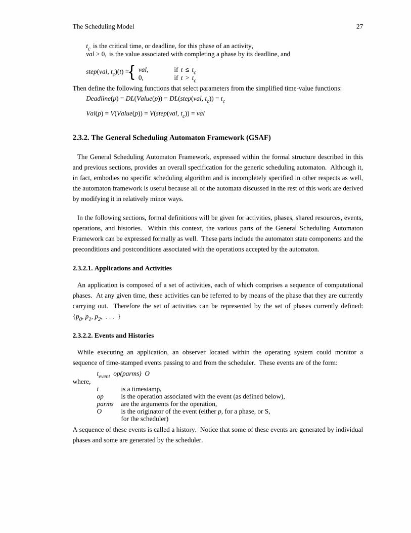
The Scheduling Model 27
t is the critical time, or deadline, for this phase of an activity,cval > 0, is the value associated with completing a phase by its deadline, and
val, if t ≤ tstep(val, t )(t) = cc { 0, if t > tcThen define the following functions that select parameters from the simplified time-value functions:
Deadline(p) = DL(Value(p)) = DL(step(val, t )) = tc c
Val(p) = V(Value(p)) = V(step(val, t )) = valc
2.3.2. The General Scheduling Automaton Framework (GSAF)
The General Scheduling Automaton Framework, expressed within the formal structure described in this
and previous sections, provides an overall specification for the generic scheduling automaton. Although it,
in fact, embodies no specific scheduling algorithm and is incompletely specified in other respects as well,
the automaton framework is useful because all of the automata discussed in the rest of this work are derived
by modifying it in relatively minor ways.
In the following sections, formal definitions will be given for activities, phases, shared resources, events,
operations, and histories. Within this context, the various parts of the General Scheduling Automaton
Framework can be expressed formally as well. These parts include the automaton state components and the
preconditions and postconditions associated with the operations accepted by the automaton.
2.3.2.1. Applications and Activities
An application is composed of a set of activities, each of which comprises a sequence of computational
phases. At any given time, these activities can be referred to by means of the phase that they are currently
carrying out. Therefore the set of activities can be represented by the set of phases currently defined:
{p , p , p , . . . }0 1 2
2.3.2.2. Events and Histories
While executing an application, an observer located within the operating system could monitor a
sequence of time-stamped events passing to and from the scheduler. These events are of the form:
t op(parms) Oeventwhere,
t is a timestamp,op is the operation associated with the event (as defined below),parms are the arguments for the operation,O is the originator of the event (either p, for a phase, or S,
for the scheduler)
A sequence of these events is called a history. Notice that some of these events are generated by individual
phases and some are generated by the scheduler.
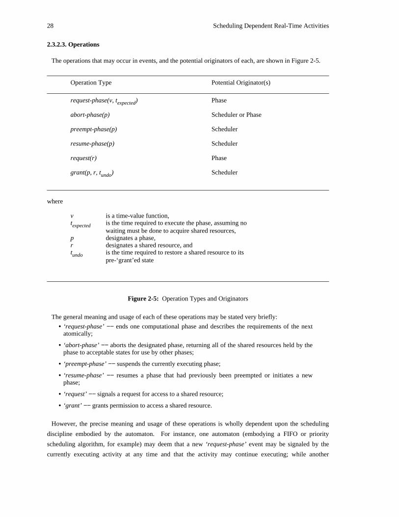
28 Scheduling Dependent Real-Time Activities
2.3.2.3. Operations
The operations that may occur in events, and the potential originators of each, are shown in Figure 2-5.
Operation Type Potential Originator(s)
request-phase(v, t ) Phaseexpected
abort-phase(p) Scheduler or Phase
preempt-phase(p) Scheduler
resume-phase(p) Scheduler
request(r) Phase
grant(p, r, t ) Schedulerundo
where
v is a time-value function,t is the time required to execute the phase, assuming noexpected
waiting must be done to acquire shared resources,p designates a phase,r designates a shared resource, andt is the time required to restore a shared resource to itsundo
pre-‘grant’ed state
Figure 2-5: Operation Types and Originators
The general meaning and usage of each of these operations may be stated very briefly:
• ‘request-phase’ −− ends one computational phase and describes the requirements of the nextatomically;
• ‘abort-phase’ −− aborts the designated phase, returning all of the shared resources held by thephase to acceptable states for use by other phases;
• ‘preempt-phase’ −− suspends the currently executing phase;
• ‘resume-phase’ −− resumes a phase that had previously been preempted or initiates a newphase;
• ‘request’ −− signals a request for access to a shared resource;
• ‘grant’ −− grants permission to access a shared resource.
However, the precise meaning and usage of these operations is wholly dependent upon the scheduling
discipline embodied by the automaton. For instance, one automaton (embodying a FIFO or priority
scheduling algorithm, for example) may deem that a new ‘request-phase’ event may be signaled by the
currently executing activity at any time and that the activity may continue executing; while another
The Scheduling Model 29
automaton (embodying the DASA scheduling algorithm, which is presented in Chapter 3) may require that
a scheduling decision must be made at that point, possibly resulting in the execution of a different activity.
Similarly, the rules for when, and even if, phases may be preempted or aborted may vary from automaton
to automaton.
Section 2.3.2.10 describes, in a little more detail, the semantics associated with these operations. Once
again, there is some vagueness due to the fact that the definition is couched in terms of an automaton
framework and not a true automaton instance. In Chapter 3, specific definitions will be presented for the
operations accepted by the DASA Scheduling Automaton.
2.3.2.4. Computational Phases of Activities
The individual computational phases that comprise an activity are delimited by ‘request-phase’ events. A
‘request-phase’ event simultaneously ends one computational phase of an activity and describes the known
requirements of the the next computational phase.
Each phase that is successfully completed contributes value to the overall application. That value is
determined by evaluating the time-value function describing the phase just completed at the time of
completion. On the other hand, an aborted computational phase contributes no value to the overall
application −− although it may free resources that allow other critical phases to execute.
2.3.2.5. Shared Resources
Phases may access shared resources. A request for such access is signaled by a phase by means of a
‘request’ event for the specific resource desired. Permission to access a shared resource is signaled to the
phase by means of a ‘grant’ event.
All shared resources that are held by an activity must be released at the completion or abortion of each
computational phase.
In addition to the identifiers that represent shared resources, there is also a special identifier, nullresource,
that does not refer to any shared resource. It has been introduced for notational convenience so that formal
definitions can refer to the nullresource to indicate that a specific phase is not currently requesting or
accessing a shared resource.
2.3.2.6. Phase Preemption and Resumption
At any given time there is one phase that is active. It may be preempted by the scheduler. This is
signaled by a ‘preempt-phase’ event. The scheduler may subsequently determine that the phase should be
resumed; this is signaled by a ‘resume-phase’ event.
The computational model allows a phase to be preempted at any time. Individual scheduling algorithms
may restrict this by only allowing preemption at specific times or by not permitting preemption at all. This
type of behavior is formally described in the precondition of the ‘preempt-phase’ event operation for each
specific scheduling automaton.
30 Scheduling Dependent Real-Time Activities
2.3.2.7. Event Terminology and Notation
Some additional terminology and notation will be useful for discussing events. Let an event, e represent
the following event:
e = t op(parms) Oevent
Then define the following simple functions:
timestamp(e) = tevent
eventtype(e) = op
source(e) = O
2.3.2.8. Definitions and Properties of Histories
Earlier, a history was defined as a sequence of events. Not all histories are meaningful or well-formed.
Let e , e , e . . . denote events. Then, formally, a history, H, can be denoted as:0 1 2
H = e ⋅ e ⋅ e ⋅ . . . ⋅ e0 1 2 n
where the operator "⋅" denotes concatenation. This notation indicates that event e appears first in history0
H, followed sequentially by the other events in the specified order. An empty history −− that is, a history
that has no events −− is denoted by the symbol "φ."
Informally, a projection of a history selects designated events from the history, preserving their relative
positions. For instance, one projection of a history could include all of the ‘request-phase’s from that
history, while another projection of the same history might include all of the events that dealt with a
specific phase. The symbol "|" denotes a projection. So for example, H | p represents the projection of
history H onto phase p. This projection would include all of the events that were originated by phase p or
that were originated by the scheduler and included p as an operational parameter. As another example, the
projection H | A represents the projection of history H onto activity A, thereby including all of the events
that involve activity A.
16The conditions that define a well-formed history include :1. event timestamps must increase monotonically and must be unique −− test: examine the
timestamps on events; for example, apply the function timestampsOK() to a history H to verifythat it meets this requirement, where timestampsOK() is defined as:
timestampsOK(φ) = timestampsOK(e) = true
timestampsOK(e ⋅e ⋅H)1 2
false, if timestamp(e ) ≥ timestamp(e )= 1 2{ timestampsOK(e ⋅H), otherwise2
16It is not always clear that a specific test be a requirement of a well-formed history or whether it is a requirement that determineswhich histories will be accepted by a given automaton. There is no question that the proper temporal ordering of events is arequirement for a well-formed history; however, tests that constrain the relative ordering of specific events −− for instance, ‘request’and ‘grant’ events −− in a history are not so obviously requirements for a well-formed history. As a result, this list is merely anattempt to lay down an initial set of tests. Some of these tests need not be done prior to submitting the history to an automaton −− inthose cases, the automaton will enforce the requirements verified by the tests in question.
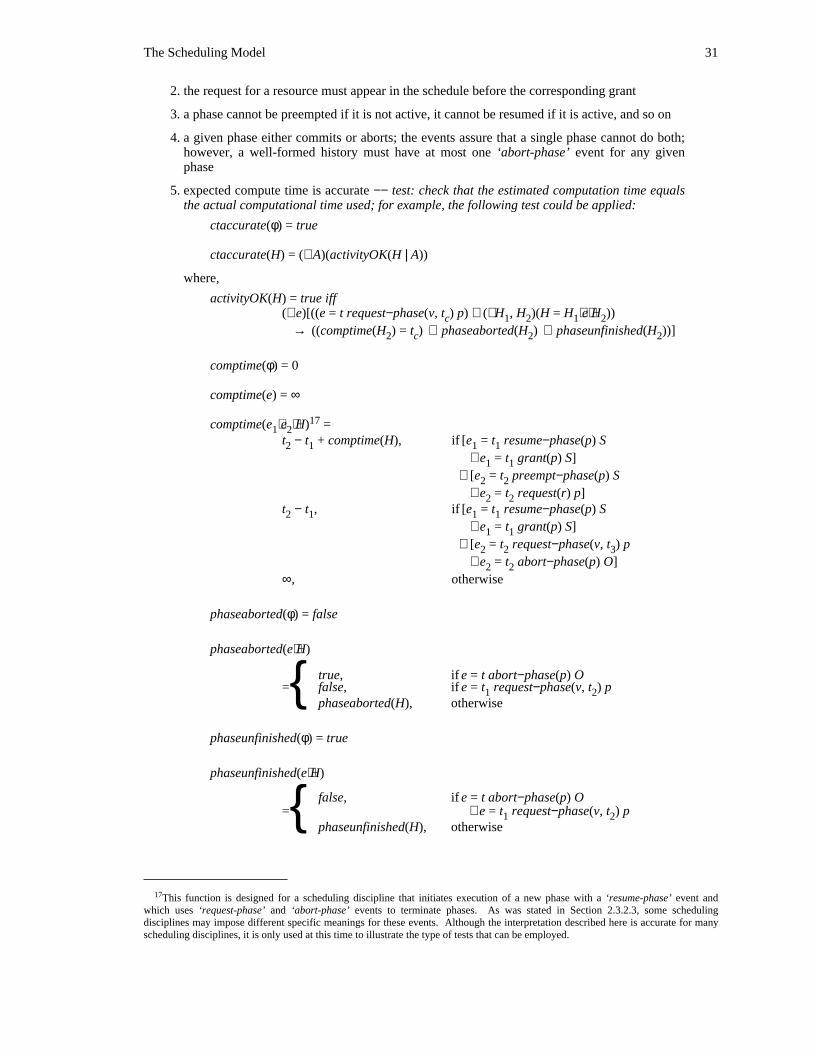
The Scheduling Model 31
2. the request for a resource must appear in the schedule before the corresponding grant
3. a phase cannot be preempted if it is not active, it cannot be resumed if it is active, and so on
4. a given phase either commits or aborts; the events assure that a single phase cannot do both;however, a well-formed history must have at most one ‘abort-phase’ event for any givenphase
5. expected compute time is accurate −− test: check that the estimated computation time equalsthe actual computational time used; for example, the following test could be applied:
ctaccurate(φ) = true
ctaccurate(H) = (∀A)(activityOK(H | A))
where,
activityOK(H) = true iff(∀e)[((e = t request−phase(v, t ) p) ∧ (∃H , H )(H = H ⋅e⋅H ))c 1 2 1 2
→ ((comptime(H ) = t ) ∨ phaseaborted(H ) ∨ phaseunfinished(H ))]2 c 2 2
comptime(φ) = 0
comptime(e) = ∞
17comptime(e ⋅e ⋅H) =1 2t − t + comptime(H), if [e = t resume−phase(p) S2 1 1 1
∨ e = t grant(p) S]1 1∧ [e = t preempt−phase(p) S2 2
∨ e = t request(r) p]2 2t − t , if [e = t resume−phase(p) S2 1 1 1
∨ e = t grant(p) S]1 1∧ [e = t request−phase(v, t ) p2 2 3
∨ e = t abort−phase(p) O]2 2∞, otherwise
phaseaborted(φ) = false
phaseaborted(e⋅H)
true, if e = t abort−phase(p) O= false, if e = t request−phase(v, t ) p1 2{
phaseaborted(H), otherwise
phaseunfinished(φ) = true
phaseunfinished(e⋅H)
false, if e = t abort−phase(p) O= ∨ e = t request−phase(v, t ) p1 2{
phaseunfinished(H), otherwise
17This function is designed for a scheduling discipline that initiates execution of a new phase with a ‘resume-phase’ event andwhich uses ‘request-phase’ and ‘abort-phase’ events to terminate phases. As was stated in Section 2.3.2.3, some schedulingdisciplines may impose different specific meanings for these events. Although the interpretation described here is accurate for manyscheduling disciplines, it is only used at this time to illustrate the type of tests that can be employed.
32 Scheduling Dependent Real-Time Activities
6. expected abort time is accurate −− test: similar to the previous test
7. estimated computation time required for a phase must always be greater than or equal to18zero
8. no ‘request’ event should request access to the nullresource
The preceding list includes tests to determine whether or not a history is well-formed with respect to
certain conditions. These tests are typical of those that may be developed to examine histories. Similar,
usually simpler, tests can be devised for all of the other conditions.
2.3.2.9. Automaton State Components
The state components associated with the General Scheduling Automaton Framework are shown in
Figure 2-6. Each component and the range of values it may take on, is described below.
ExecMode. ExecMode is a relation that associates an execution mode with each phase. At any given
time, a phase can be either executing normally or aborting. Also at any time, a normally executing phase
can be aborted. Once an abort is initiated, it must be completed before normal execution of the entire phase
can again be attempted.
ExecClock and AbortClock. The next two state components shown in Figure 2-6 are used to track the
amount of time required to complete the normal execution or the abortion of a phase. When a phase is
executing normally, the relation ExecClock indicates the amount of processing time needed to successfully
complete the execution of that phase. Similarly, when a phase is aborting, AbortClock indicates the amount
of processing time needed to complete the abort processing.
At the start of a new phase, ExecClock associates a value provided by the activity with the phase. If the20phase was executed in isolation , ExecClock specifies the amount of time that would elapse before the
phase would complete executing. Each time the phase executes, the value of ExecClock for that phase
decreases. When it reaches zero, then the phase has completed execution.
On the other hand, AbortClock represents the time required to abort the current phase. In addition, the
exact length of time required to abort the phase depends on the number and type of shared resources that it
has acquired. Therefore, since no shared resources have yet been acquired, AbortClock is zero at the start
of every phase. Subsequently, after any shared resource is requested and granted, the value of AbortClock
is incremented by an amount that is a function of that resource. This amount of time has been chosen to
allow the shared resource to be returned to an acceptable state so that other phases may use it.
18An additional requirement may also be placed on the parameters of a ‘request-phase’ event: the value function must be of theappropriate form, as outlined below. This requirement has not been included in this list because the tests that are present all apply tothe general case of scheduling with dependency considerations in a real-time environment using information available from arbitrarytime-value functions. This requirement is related to a simplification made to make the work more clear and more manageable, and sodoes not seem to carry the same weight as the others listed above.
20By executing in isolation, contention with other activities for both processor cycles and shared resources is eliminated. In fact, thephase does not execute in isolation and these factors cannot be ignored −− leading to this scheduling work.
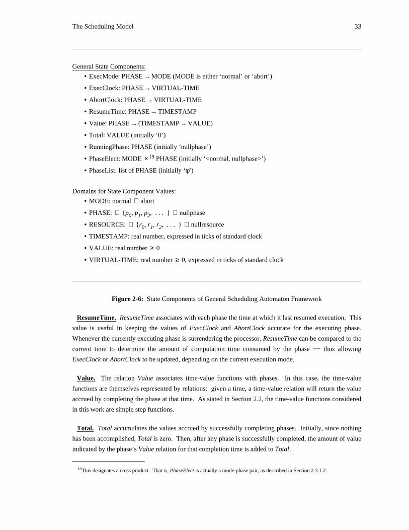
The Scheduling Model 33
General State Components:
• ExecMode: PHASE → MODE (MODE is either ‘normal’ or ‘abort’)
• ExecClock: PHASE → VIRTUAL-TIME
• AbortClock: PHASE → VIRTUAL-TIME
• ResumeTime: PHASE → TIMESTAMP
• Value: PHASE → (TIMESTAMP → VALUE)
• Total: VALUE (initially ‘0’)
• RunningPhase: PHASE (initially ‘nullphase’)
19• PhaseElect: MODE × PHASE (initially ‘<normal, nullphase>’)
• PhaseList: list of PHASE (initially ‘φ’)
Domains for State Component Values:
• MODE: normal ∨ abort
• PHASE: ∈ {p , p , p , . . . } ∨ nullphase0 1 2
• RESOURCE: ∈ {r , r , r , . . . } ∨ nullresource0 1 2
• TIMESTAMP: real number, expressed in ticks of standard clock
• VALUE: real number ≥ 0
• VIRTUAL-TIME: real number ≥ 0, expressed in ticks of standard clock
Figure 2-6: State Components of General Scheduling Automaton Framework
ResumeTime. ResumeTime associates with each phase the time at which it last resumed execution. This
value is useful in keeping the values of ExecClock and AbortClock accurate for the executing phase.
Whenever the currently executing phase is surrendering the processor, ResumeTime can be compared to the
current time to determine the amount of computation time consumed by the phase −− thus allowing
ExecClock or AbortClock to be updated, depending on the current execution mode.
Value. The relation Value associates time-value functions with phases. In this case, the time-value
functions are themselves represented by relations: given a time, a time-value relation will return the value
accrued by completing the phase at that time. As stated in Section 2.2, the time-value functions considered
in this work are simple step functions.
Total. Total accumulates the values accrued by successfully completing phases. Initially, since nothing
has been accomplished, Total is zero. Then, after any phase is successfully completed, the amount of value
indicated by the phase’s Value relation for that completion time is added to Total.
19This designates a cross product. That is, PhaseElect is actually a mode-phase pair, as described in Section 2.3.1.2.

34 Scheduling Dependent Real-Time Activities
The values of the Total state components of two different scheduling automata that have worked on the
same application can be compared to determine which yielded a higher total value for the application.
(This fact will be used in simulations and proofs in later chapters when comparing two different scheduling
algorithms.)
RunningPhase. RunningPhase indicates which phase is currently executing on the processor. If no
activity is currently executing −− as is the case initially −− RunningPhase is equal to nullphase.
PhaseElect. PhaseElect also indicates a phase. In this case, it is the phase that should be executing now.
If this is different than RunningPhase, then the currently executing phase should be suspended and replaced
by the PhaseElect. Once again, in the initially empty system, PhaseElect specifies that the nullphase
should be executed normally.
PhaseElect names not only the phase to be executed but also the execution mode for the phase.
PhaseList. PhaseList is simply a list containing all of the phases known to the automaton. This list
changes as new phases arrive and old phases are completed. Initially, since there are no phases PhaseList
is empty.
Automaton-Specific State Components. Other state components are also associated with an automaton.
These are used to handle some of the bookkeeping details for the specific scheduler being used. The
components that appear above are intended to reflect the state that any specific scheduler would need and
maintain under this general model.
Specific initial values may be given to many of these state components in order to satisfy the
requirements of a given automaton.
Domains for State Component Values. The domains that supply the values for the state components
are straightforward and are shown in Figure 2-6 along with the state components of the General Scheduling
Automaton Framework. The domain MODE contains only two values: normal and abort. The domain
PHASE consists of all of the phases known by the automaton as well as the nullphase. Similarly, the domain
RESOURCE consists of all of the shared resources known to the automaton as well as the nullresource. The
values from all of the time-value functions are drawn from the domain VALUE. These must be positive
(according to the assumptions stated earlier in Section 2.3.1.3) and are chosen from the real numbers so that
there are no unnecessary restrictions placed on them. The domain VALUE also contains zero since Total
receives its value from this domain and it initially has no accrued value.
Time is central to the behavior of real-time systems, and the domain TIMESTAMPS provides a source of
markers in time for the automaton to use. Each timestamp is expressed in terms of ticks of a standard
clock. The ticks of this clock are equally spaced in time; and in fact, nothing in the model prevents the
timestamps from taking on fractional numbers of ticks −− thus allowing arbitrarily great precision to be
obtained in representation of times.
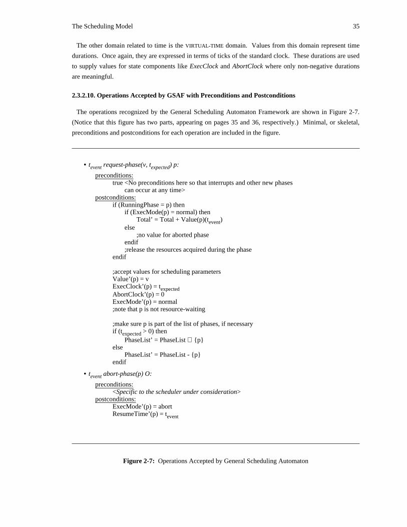
The Scheduling Model 35
The other domain related to time is the VIRTUAL-TIME domain. Values from this domain represent time
durations. Once again, they are expressed in terms of ticks of the standard clock. These durations are used
to supply values for state components like ExecClock and AbortClock where only non-negative durations
are meaningful.
2.3.2.10. Operations Accepted by GSAF with Preconditions and Postconditions
The operations recognized by the General Scheduling Automaton Framework are shown in Figure 2-7.
(Notice that this figure has two parts, appearing on pages 35 and 36, respectively.) Minimal, or skeletal,
preconditions and postconditions for each operation are included in the figure.
• t request-phase(v, t ) p:event expected
preconditions:true <No preconditions here so that interrupts and other new phases
can occur at any time>postconditions:
if (RunningPhase = p) thenif (ExecMode(p) = normal) then
Total’ = Total + Value(p)(t )eventelse
;no value for aborted phaseendif;release the resources acquired during the phase
endif
;accept values for scheduling parametersValue’(p) = vExecClock’(p) = texpectedAbortClock’(p) = 0ExecMode’(p) = normal;note that p is not resource-waiting
;make sure p is part of the list of phases, if necessaryif (t > 0) thenexpected
PhaseList’ = PhaseList ∪ {p}else
PhaseList’ = PhaseList - {p}endif
• t abort-phase(p) O:event
preconditions:<Specific to the scheduler under consideration>
postconditions:ExecMode’(p) = abortResumeTime’(p) = tevent
Figure 2-7: Operations Accepted by General Scheduling Automaton
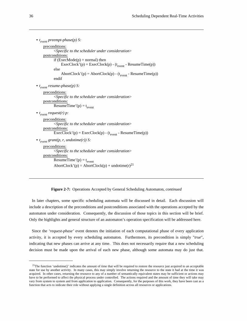
36 Scheduling Dependent Real-Time Activities
• t preempt-phase(p) S:event
preconditions:<Specific to the scheduler under consideration>
postconditions:if (ExecMode(p) = normal) then
ExecClock’(p) = ExecClock(p) - (t - ResumeTime(p))eventelse
AbortClock’(p) = AbortClock(p) - (t - ResumeTime(p))eventendif
• t resume-phase(p) S:event
preconditions:<Specific to the scheduler under consideration>
postconditions:ResumeTime’(p) = tevent
• t request(r) p:event
preconditions:<Specific to the scheduler under consideration>
postconditions:ExecClock’(p) = ExecClock(p) - (t - ResumeTime(p))event
• t grant(p, r, undotime(r)) S:event
preconditions:<Specific to the scheduler under consideration>
postconditions:ResumeTime’(p) = tevent
21AbortClock’(p) = AbortClock(p) + undotime(r)
Figure 2-7: Operations Accepted by General Scheduling Automaton, continued
In later chapters, some specific scheduling automata will be discussed in detail. Each discussion will
include a description of the preconditions and postconditions associated with the operations accepted by the
automaton under consideration. Consequently, the discussion of those topics in this section will be brief.
Only the highlights and general structure of an automaton’s operation specification will be addressed here.
Since the ‘request-phase’ event denotes the initiation of each computational phase of every application
activity, it is accepted by every scheduling automaton. Furthermore, its precondition is simply "true",
indicating that new phases can arrive at any time. This does not necessarily require that a new scheduling
decision must be made upon the arrival of each new phase, although some automata may do just that.
21The function ‘undotime()’ indicates the amount of time that will be required to restore the resource just acquired to an acceptablestate for use by another activity. In many cases, this may simply involve returning the resource to the state it had at the time it wasacquired. In other cases, returning the resource to any of a number of semantically equivalent states may be sufficient or actions mayhave to be performed to affect the physical process under controlled. The actions required and the amount of time they will take mayvary from system to system and from application to application. Consequently, for the purposes of this work, they have been cast as afunction that acts to indicate their role without applying a single definition across all resources or applications.
The Scheduling Model 37
Since such a scheduling decision is not made in every scheduling automaton, no decision is made in the
General Scheduling Automata Framework.
In the same spirit, the postconditions for the ‘request-phase’ event include only those conditions that will
almost certainly belong in every scheduling automaton of interest. Those postconditions: (1) accumulate
any value accrued from completing a previous computational phase of the same activity; (2) initialize the
automaton’s state components to capture the new phase’s scheduling parameters; and (3) update the list of
phases known to the automaton based on the new phase’s scheduling parameters.
Notice that value is accumulated for the completion of a previous phase only if the currently executing
phase issues the ‘request-phase’ event, thereby signaling that the current phase has completed execution. If
some other activity issues the ‘request-phase’ event, it is signaling the existence of a new phase to the
automaton while a different phase is executing, so no phase completion has occurred.
In addition, no value is accrued for a phase that has been aborted. If, on the other hand, the phase has
completed successfully the value accrued is determined by evaluating its time-value function at the time of
completion.
Finally, since it requires a positive amount of time to accomplish any processing, a t parameter thatexpected
is less than or equal to zero indicates that there is no subsequent computational phase for the activity
issuing the ‘request-phase’ event. In that case, the phase is removed from the PhaseList; in all other cases,
the phase is included in the PhaseList.
The ‘abort-phase’ event in the General Scheduling Automaton Framework is similar to the remainder of
the scheduling events: its precondition is automaton-specific and its postconditions specify bookkeeping
that must be done in the event that the event occurs. In particular, the ‘abort-phase’ event’s postconditions
change the phase’s execution mode to abort and note the time that the phase began aborting. In the event
of a preemption, this time (ResumeTime) will be consulted to adjust the phase’s AbortClock to indicate the
amount of time required to complete the abort processing, which will be used in subsequent scheduling
decisions.
The ‘preempt-phase’ event has an automaton-specific precondition. Its postconditions handle the
bookkeeping associated with preempting the executing phase. Specifically, ExecClock or AbortClock is
updated to reflect the amount of time still required to complete the normal or abort processing of the phase,
respectively. This is accomplished by subtracting the amount of time the phase had executed prior to the
preemption from the amount of time it still needed to complete processing before it began that execution.
A ‘resume-phase’ event is used to resume execution of a phase that had been suspended by a
‘preempt-phase’ event. The ‘resume-phase’ event, which has an automaton-specific precondition, simply
notes the time at which the designated phase resumed execution. This time is used to adjust the state
components dealing with the required execution time of the phase whenever the phase is subsequently
preempted.
38 Scheduling Dependent Real-Time Activities
Once again, the ‘request’ event has an automaton-specific precondition. Its postcondition updates the
appropriate state component clock for the phase, depending on its execution mode. This is done to
facilitate the use of a scheduling decision as a result of a request for a shared resource. The updating of the
relevant state components ensures that the automaton will make a decision based on the most up-to-date
information.
The ‘grant’ event, which also has an automaton-specific precondition, notes the time at which the phase
is awarded the shared resource it had previously requested and begins execution. Another postcondition
increments the AbortClock state component for the designated phase to reflect the amount of time that will
be required to return the shared resource to an acceptable state for another phase in the event that the
current phase is aborted. This length of time may vary from resource to resource, and so is denoted as
undotime(r), a function of the resource in question.
Although the ‘request’ and ‘grant’ phase events behave as if the processor is surrendered after each
request, this does not have to be the case. The ‘request’ event can be immediately followed by the
corresponding ‘grant’ event to model the situation in which the processor is not surrendered.
Typeface Convention. In the definition of the GSAF, all of the operation definitions −− that is, all of the
the operations’ preconditions and postconditions −− have been presented in a roman (upright) typeface. In
the future, when automata are presented, those parts that are common with the GSAF will continue to be
written in a roman typeface. However, those parts that are different will be written in an italic typeface.
This will allow the reader to focus on those parts of the definition that are different from the general
framework.
2.3.2.11. Active Phase Selection
Although the General Scheduling Automaton Framework contains state components and will accept some
scheduling events, it is not really a scheduling automaton. Rather, it is a framework: a skeleton that has
most, but not all, of the elements of a scheduling automaton. For instance, as was discussed in the previous
section (Section 2.3.2.10), most of the preconditions for accepting various scheduling events are
unspecified in the General Scheduling Automaton Framework. Also, while some postconditions have been
specified, they have not been completely specified.
Another of the more noticeable omissions in the specification of the General Scheduling Automaton
Framework is the lack of a function to select the next phase to execute. Furthermore, not only is this
function not specified, the places in the automaton where it is to be invoked are also unspecified. This is
because different schedulers invoke this function at different times. Therefore, there is no canonical set of
times (corresponding to a fixed set of points in the General Scheduling Automaton Framework) where all
scheduling algorithms invoke a phase selection function. As a result, this has been omitted from the
General Scheduling Automaton Framework, which acts as a lowest common denominator of sorts among
instance of scheduling automata.
To illustrate this point, consider two simple scheduling algorithms: FIFO scheduling and priority
The Scheduling Model 39
scheduling. Whenever a new computational phase enters the system −− as indicated by a new
‘request-phase’ event −− the FIFO scheduling automaton will note that fact, but will not invoke a phase
selection function to determine what phase to execute. It simply allows the currently executing phase to
proceed until it gives up the processor.
On the other hand, the priority scheduling automaton will make a new determination concerning which
phase to execute: if the new computational phase has a higher priority than the currently executing phase,
then the active phase is preempted in favor of the new phase.
More complex scheduling algorithms may evaluate the phase selection function at other times as well.
For instance, the DASA algorithm described in Chapter 3 invokes the phase selection function whenever a
shared resource is requested by any phase. It is also conceivable that there are schedulers that might select
which phase to run asynchronously with respect to the given set of scheduler operations. For example, a
round robin scheduler that gave each phase a turn by offering it a time-slice would make preemption
decisions following evenly spaced clock interrupts. To accommodate such extensions, new scheduling
operations would have to be added to the model. While that is straightforward, it is not required to
investigate the algorithms of interest for scheduling supervisory control systems, and so it would only serve
to complicate the model. Consequently, the scheduling operations included in the model represent a
minimal set that captures all of the relevant behavior within supervisory control systems.
2.3.3. Notes
The following paragraphs address some additional points concerning the GSAF framework. These points
generally explain how facets of real applications are, or can be, reflected in the formal model.
2.3.3.1. Manifestation of Assumptions and Restrictions
Section 2.2 describes the specific assumptions and restrictions that are employed in this work. A look at
the GSAF framework will reveal how those assumptions are manifest.
The first assumption stated that all time-value functions are restricted to be simple step functions. The
definition provided for time-value functions in the model in Section 2.3.1.3 captures that assumption
directly.
The second assumption stated that the computation time required by an activity to complete a
computational phase is accurately known. This is reflected in the ‘request-phase’ operation itself. The
operation includes a parameter that informs the scheduler of the required computation time. (See the
description of the operation and its parameters in Section 2.3.2.3 or Section 2.3.2.10.)
This information is then available for use by the scheduling algorithm embodied in a given scheduling
automaton. Although the GSAF framework presented in this chapter does not use this information, other
automata may.
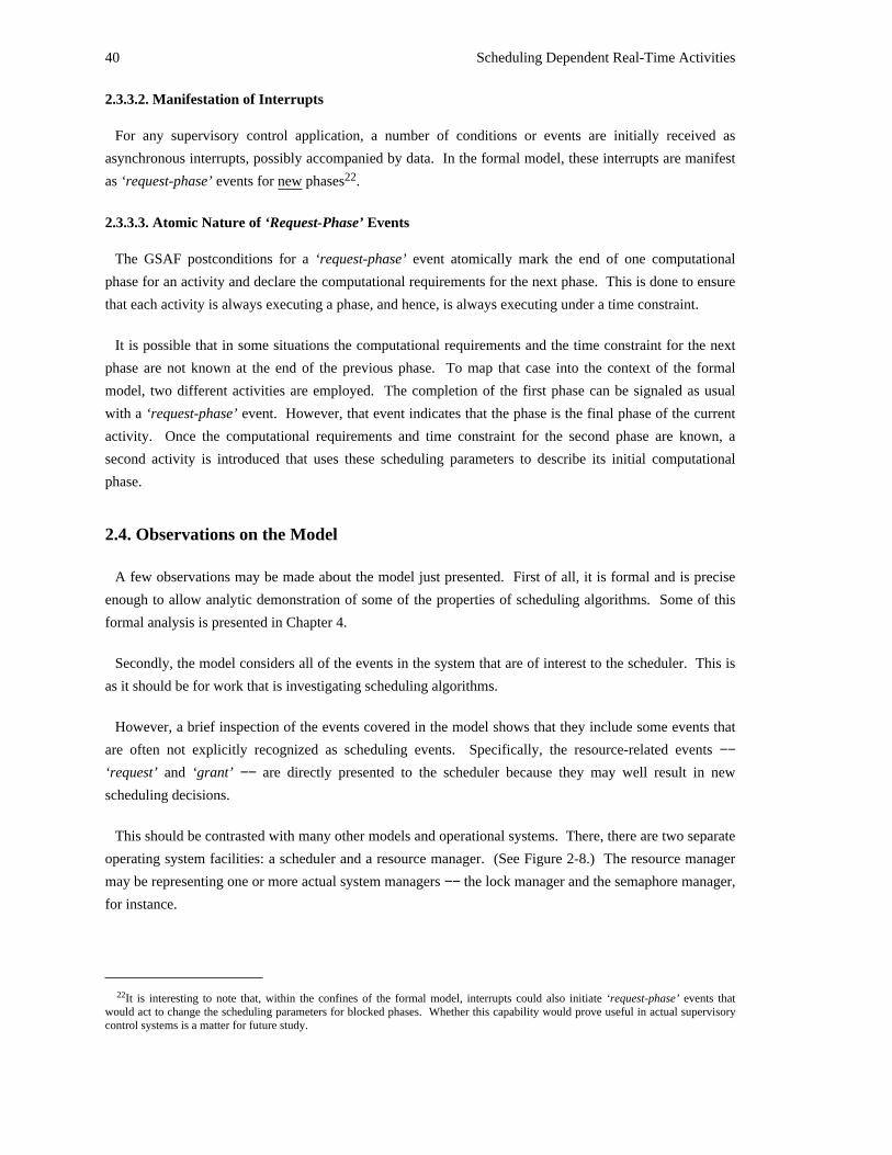
40 Scheduling Dependent Real-Time Activities
2.3.3.2. Manifestation of Interrupts
For any supervisory control application, a number of conditions or events are initially received as
asynchronous interrupts, possibly accompanied by data. In the formal model, these interrupts are manifest22as ‘request-phase’ events for new phases .
2.3.3.3. Atomic Nature of ‘Request-Phase’ Events
The GSAF postconditions for a ‘request-phase’ event atomically mark the end of one computational
phase for an activity and declare the computational requirements for the next phase. This is done to ensure
that each activity is always executing a phase, and hence, is always executing under a time constraint.
It is possible that in some situations the computational requirements and the time constraint for the next
phase are not known at the end of the previous phase. To map that case into the context of the formal
model, two different activities are employed. The completion of the first phase can be signaled as usual
with a ‘request-phase’ event. However, that event indicates that the phase is the final phase of the current
activity. Once the computational requirements and time constraint for the second phase are known, a
second activity is introduced that uses these scheduling parameters to describe its initial computational
phase.
2.4. Observations on the Model
A few observations may be made about the model just presented. First of all, it is formal and is precise
enough to allow analytic demonstration of some of the properties of scheduling algorithms. Some of this
formal analysis is presented in Chapter 4.
Secondly, the model considers all of the events in the system that are of interest to the scheduler. This is
as it should be for work that is investigating scheduling algorithms.
However, a brief inspection of the events covered in the model shows that they include some events that
are often not explicitly recognized as scheduling events. Specifically, the resource-related events −−‘request’ and ‘grant’ −− are directly presented to the scheduler because they may well result in new
scheduling decisions.
This should be contrasted with many other models and operational systems. There, there are two separate
operating system facilities: a scheduler and a resource manager. (See Figure 2-8.) The resource manager
may be representing one or more actual system managers −− the lock manager and the semaphore manager,
for instance.
22It is interesting to note that, within the confines of the formal model, interrupts could also initiate ‘request-phase’ events thatwould act to change the scheduling parameters for blocked phases. Whether this capability would prove useful in actual supervisorycontrol systems is a matter for future study.
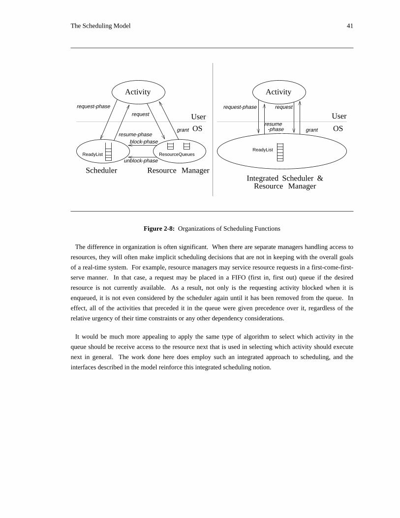
The Scheduling Model 41
User
OS
Integrated Scheduler &Resource Manager
request-phase
resumegrant
block-phase
unblock-phase
User
OS
Scheduler Resource Manager
Activity
request-phase
resume-phase
request
grant
Activity
request
-phase
ReadyListResourceQueuesReadyList
Figure 2-8: Organizations of Scheduling Functions
The difference in organization is often significant. When there are separate managers handling access to
resources, they will often make implicit scheduling decisions that are not in keeping with the overall goals
of a real-time system. For example, resource managers may service resource requests in a first-come-first-
serve manner. In that case, a request may be placed in a FIFO (first in, first out) queue if the desired
resource is not currently available. As a result, not only is the requesting activity blocked when it is
enqueued, it is not even considered by the scheduler again until it has been removed from the queue. In
effect, all of the activities that preceded it in the queue were given precedence over it, regardless of the
relative urgency of their time constraints or any other dependency considerations.
It would be much more appealing to apply the same type of algorithm to select which activity in the
queue should be receive access to the resource next that is used in selecting which activity should execute
next in general. The work done here does employ such an integrated approach to scheduling, and the
interfaces described in the model reinforce this integrated scheduling notion.

42 Scheduling Dependent Real-Time Activities
Chapter 3
The DASA Algorithm
The algorithm investigated in this thesis is called DASA (Dependent Activity Scheduling Algorithm). It
addresses the dependency concerns described in the previous chapters in a clear and natural manner. The
algorithm is based on a set of heuristics that deliver the type of behavior required in real-time systems,
particularly supervisory control systems.
This chapter presents the DASA algorithm. First, DASA is described in general terms, placing emphasis on
the rationale for the algorithm. Then a formal definition is presented, providing a framework for careful
analysis of the algorithm. Finally, the scheduling example from Section 1.3 is revisited. This time the
DASA algorithm is employed to make the scheduling decisions, thereby contrasting its behavior with that of
the algorithms previously mentioned.
3.1. Dependent Activity Scheduling Algorithm
This section describes the underlying heuristics for the DASA algorithm, along with the rationale for their
adoption, in order to explain its high level goals. This discussion is followed by an informal definition of
the DASA algorithm. (The next section, Section 3.2, provides the formal definition.)
3.1.1. Heuristics and Rationale
The DASA algorithm was constructed to possess a number of properties, each of which has appeal on its
own merits. Taken together, they suggest that the algorithm may be quite effective in handling scheduling
problems with dependency considerations.
Before looking at the definition of the DASA algorithm, two important metrics must be understood. These
are the notions of value density [Locke 86] and potential value density. Value density is a measure of how
much value (as defined by the application) per unit time will be acquired by executing a single
computational phase. In the cases considered by this thesis, where time-value functions are simply step
functions, the value density is the height of the step function −− the value −− divided by the required23computation time .
23In more complex cases, more involved time-value functions and less exact knowledge of required computation time may beconsidered. These considerations will require a more complicated procedure to determine the value density based on the probabilityof completing the phase at any given instant, weighted by the height of the time-value function at that instant.
43
44 Scheduling Dependent Real-Time Activities
The potential value density of a phase extends the notion of value density to include both the designated
phase and the set of phases on which it depends. In fact, the potential value density of such a collection of
phases is the total of their individual values divided by the total of their required computation times. The
choice to add both the values and the times of the individual phases prior to performing the division to
determine the potential value density, rather than combining this information in some other way, reflects
the fact that executing the sequence of phases will require a total time equal to the sum of the individual
times and will yield a total value equal to the sum of the individual values. Therefore, the aggregate24execution sequence can accurately be characterized by the value density computed based on these sums .
Furthermore, phases that are being aborted are handled differently than those that are executing normally
when calculating a potential value density: an aborting phase contributes no value, but does require
computation time. Therefore, aborting a computation will always act to reduce the potential value density
of a collection of phases. Nonetheless, aborts may be advantageous in that they may greatly reduce the
delay that must be incurred before starting the execution of a designated computation.
With these metrics in mind, the properties desired for the DASA algorithm can be reviewed:1. explicitly account for dependencies −− account (in terms of both required computation time
and in available potential value) for each phase, along with all of the other phases on which itdepends;
2. minimize effort −− apply the minimum amount of effort necessary to allow a phase to bescheduled, possibly using aborts to expedite the process;
3. maximize return (or benefit) −− examine phases in order of decreasing potential valuedensity, thereby always obtaining the greatest return (in application-defined value) on a giveninvestment (of computation time);
4. maximize the chance of meeting deadlines −− approximate a deadline scheduler insofar aspossible;
5. globally optimize schedule −− review the schedule constructed incrementally and removeredundant or unnecessary steps.
3.1.2. Informal Definition of DASA
The DASA Dependency Scheduling Algorithm, when given a set of phases and their scheduling
parameters, will select the next phase to be executed in accordance with the heuristics just presented. This
dependency scheduling algorithm is presented in the following section.
Since mutual dependencies among activities may arise during the course of execution, care must be taken25to detect and resolve deadlocks before applying the DASA scheduling algorithm . While this thesis focuses
on the scheduling algorithm, deadlock handling is discussed briefly in Section 3.1.2.2.
24The word "potential" is used to qualify "value density" because, due to the potential for interaction among phases, it is not trulyknown that spending the indicated total number of cycles will yield the indicated total value. Unanticipated interactions could negatethe chance to acquire any value from the aggregate computation. Thus, the calculated value may only potentially result from theexecution sequence.
25Of course, there are a number of deadlock avoidance techniques that may be used as well, but it cannot be assumed that they canwork for all applications.
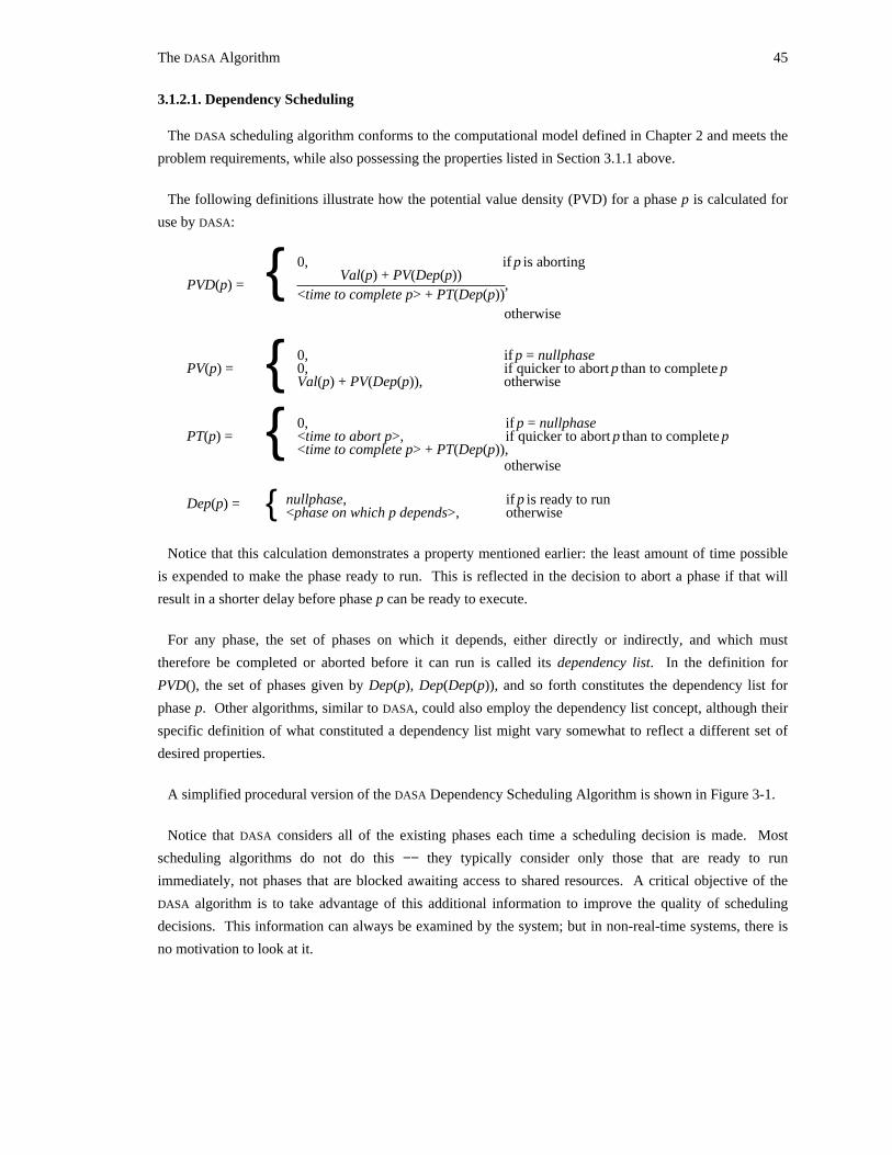
The DASA Algorithm 45
3.1.2.1. Dependency Scheduling
The DASA scheduling algorithm conforms to the computational model defined in Chapter 2 and meets the
problem requirements, while also possessing the properties listed in Section 3.1.1 above.
The following definitions illustrate how the potential value density (PVD) for a phase p is calculated for
use by DASA:
0, if p is abortingVal(p) + PV(Dep(p))
PVD(p) = { ,<time to complete p> + PT(Dep(p))
otherwise
0, if p = nullphasePV(p) = 0, if quicker to abort p than to complete p{ Val(p) + PV(Dep(p)), otherwise
0, if p = nullphasePT(p) = <time to abort p>, if quicker to abort p than to complete p{ <time to complete p> + PT(Dep(p)),
otherwise
nullphase, if p is ready to runDep(p) = { <phase on which p depends>, otherwise
Notice that this calculation demonstrates a property mentioned earlier: the least amount of time possible
is expended to make the phase ready to run. This is reflected in the decision to abort a phase if that will
result in a shorter delay before phase p can be ready to execute.
For any phase, the set of phases on which it depends, either directly or indirectly, and which must
therefore be completed or aborted before it can run is called its dependency list. In the definition for
PVD(), the set of phases given by Dep(p), Dep(Dep(p)), and so forth constitutes the dependency list for
phase p. Other algorithms, similar to DASA, could also employ the dependency list concept, although their
specific definition of what constituted a dependency list might vary somewhat to reflect a different set of
desired properties.
A simplified procedural version of the DASA Dependency Scheduling Algorithm is shown in Figure 3-1.
Notice that DASA considers all of the existing phases each time a scheduling decision is made. Most
scheduling algorithms do not do this −− they typically consider only those that are ready to run
immediately, not phases that are blocked awaiting access to shared resources. A critical objective of the
DASA algorithm is to take advantage of this additional information to improve the quality of scheduling
decisions. This information can always be examined by the system; but in non-real-time systems, there is
no motivation to look at it.
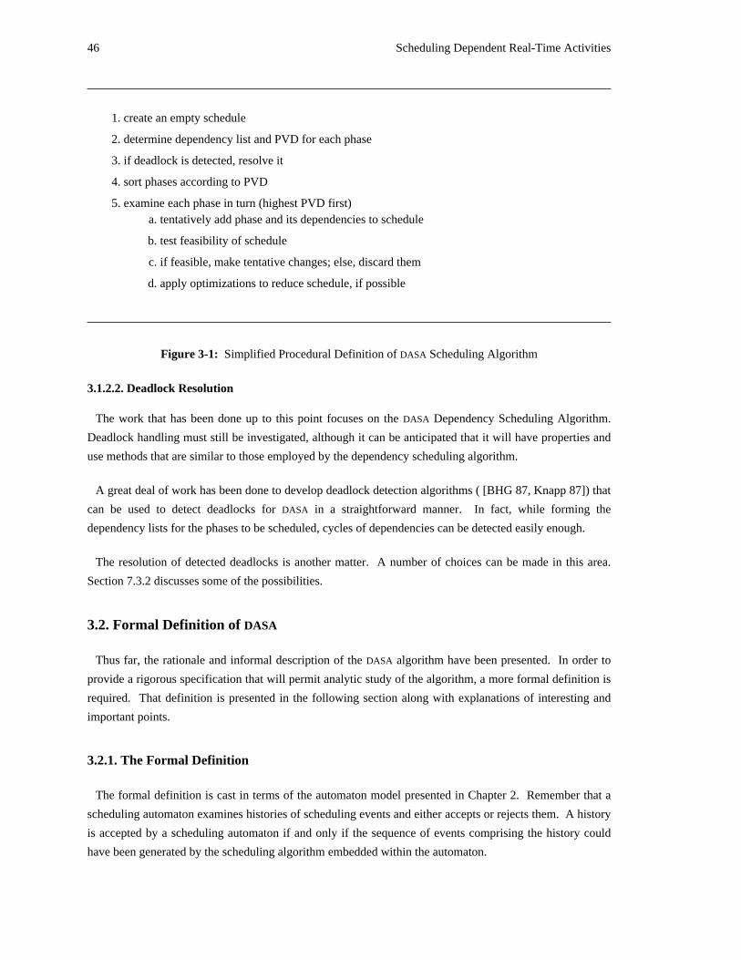
46 Scheduling Dependent Real-Time Activities
1. create an empty schedule
2. determine dependency list and PVD for each phase
3. if deadlock is detected, resolve it
4. sort phases according to PVD
5. examine each phase in turn (highest PVD first)a. tentatively add phase and its dependencies to schedule
b. test feasibility of schedule
c. if feasible, make tentative changes; else, discard them
d. apply optimizations to reduce schedule, if possible
Figure 3-1: Simplified Procedural Definition of DASA Scheduling Algorithm
3.1.2.2. Deadlock Resolution
The work that has been done up to this point focuses on the DASA Dependency Scheduling Algorithm.
Deadlock handling must still be investigated, although it can be anticipated that it will have properties and
use methods that are similar to those employed by the dependency scheduling algorithm.
A great deal of work has been done to develop deadlock detection algorithms ( [BHG 87, Knapp 87]) that
can be used to detect deadlocks for DASA in a straightforward manner. In fact, while forming the
dependency lists for the phases to be scheduled, cycles of dependencies can be detected easily enough.
The resolution of detected deadlocks is another matter. A number of choices can be made in this area.
Section 7.3.2 discusses some of the possibilities.
3.2. Formal Definition of DASA
Thus far, the rationale and informal description of the DASA algorithm have been presented. In order to
provide a rigorous specification that will permit analytic study of the algorithm, a more formal definition is
required. That definition is presented in the following section along with explanations of interesting and
important points.
3.2.1. The Formal Definition
The formal definition is cast in terms of the automaton model presented in Chapter 2. Remember that a
scheduling automaton examines histories of scheduling events and either accepts or rejects them. A history
is accepted by a scheduling automaton if and only if the sequence of events comprising the history could
have been generated by the scheduling algorithm embedded within the automaton.
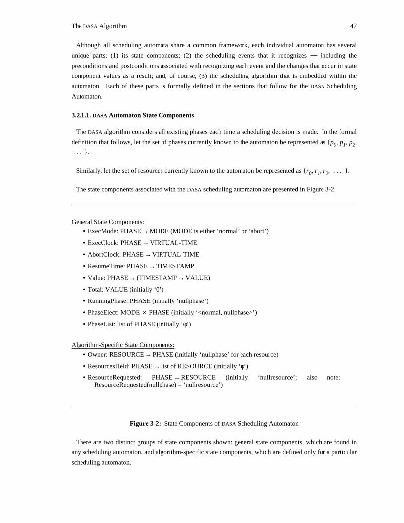
The DASA Algorithm 47
Although all scheduling automata share a common framework, each individual automaton has several
unique parts: (1) its state components; (2) the scheduling events that it recognizes −− including the
preconditions and postconditions associated with recognizing each event and the changes that occur in state
component values as a result; and, of course, (3) the scheduling algorithm that is embedded within the
automaton. Each of these parts is formally defined in the sections that follow for the DASA Scheduling
Automaton.
3.2.1.1. DASA Automaton State Components
The DASA algorithm considers all existing phases each time a scheduling decision is made. In the formal
definition that follows, let the set of phases currently known to the automaton be represented as {p , p , p ,0 1 2
. . . }.
Similarly, let the set of resources currently known to the automaton be represented as {r , r , r , . . . }.0 1 2
The state components associated with the DASA scheduling automaton are presented in Figure 3-2.
General State Components:
• ExecMode: PHASE → MODE (MODE is either ‘normal’ or ‘abort’)
• ExecClock: PHASE → VIRTUAL-TIME
• AbortClock: PHASE → VIRTUAL-TIME
• ResumeTime: PHASE → TIMESTAMP
• Value: PHASE → (TIMESTAMP → VALUE)
• Total: VALUE (initially ‘0’)
• RunningPhase: PHASE (initially ‘nullphase’)
• PhaseElect: MODE × PHASE (initially ‘<normal, nullphase>’)
• PhaseList: list of PHASE (initially ‘φ’)
Algorithm-Specific State Components:
• Owner: RESOURCE → PHASE (initially ‘nullphase’ for each resource)
• ResourcesHeld: PHASE → list of RESOURCE (initially ‘φ’)
• ResourceRequested: PHASE → RESOURCE (initially ‘nullresource’; also note:ResourceRequested(nullphase) = ‘nullresource’)
Figure 3-2: State Components of DASA Scheduling Automaton
There are two distinct groups of state components shown: general state components, which are found in
any scheduling automaton, and algorithm-specific state components, which are defined only for a particular
scheduling automaton.
48 Scheduling Dependent Real-Time Activities
The general state components were discussed in Chapter 2. They include a number of components that
describe important characteristics of each individual phase (ExecMode, ExecClock, AbortClock,
ResumeTime, and Value), as well as components that indicate the status of the automaton itself (Total,
RunningPhase, PhaseElect, and PhaseList).
All of the algorithm-specific state components of the DASA Scheduling Automaton deal with requesting
and holding shared resources. The relation Owner indicates which, if any, phase currently possesses each
of the shared resources. The Owner of all unassigned resources is nullphase. The ResourcesHeld relation
associates with each phase the list of resources that have been granted to that phase. And finally, the
ResourceRequested relation specifies which resource a given phase desires. Whenever, there is no
unsatisfied resource request for a phase, the corresponding ResourceRequested value is nullresource.
The bottom portion of Figure 3-2 defines the values that each of the state components may assume. All
of these are general value domains that were discussed when the scheduling automaton model was
presented in Chapter 2. They are repeated here only for convenience −− they allow the relation definitions
to appear in context so that earlier material need not be consulted.
An initial value is shown for many of the state components. These values indicate that, at the outset,
there are no phases known to the automaton, no value has been accrued, all of the shared resources are
available, and the processor is idle. Each of the relations that provide information for each phase in the
system is initially empty since there are no phases. As phases arrive (indicated by issuing ‘request-phase’
events), entries are made in each of these relations.
Access Queues for Resources. There is one state component that, although not present in the DASA
Scheduling Automaton, is commonly found in other scheduling automata for this problem domain: a
relation that, given a resource, specifies the queue of phases that are waiting for access to the resource.
That state component is not found in this automaton because it tends to reflect an ordering among pending
requests for a shared resource −− for example, requesters may be served in a FIFO fashion or according to
their priority. While the DASA algorithm will in some sense order such requests, it is done in a completely
dynamic fashion. The needs of each phase, including access to shared resources, are considered along with
the benefit of executing the phase each time a scheduling decision is made.
3.2.1.2. Operations Accepted by DASA Automaton
The operations recognized by the DASA scheduling automaton and their preconditions and postconditions
are shown in Figures 3-3, 3-4, and 3-5. Figure 3-3 presents the ‘request-phase’ operation, which is used to
initiate each computational phase of the activities comprising the application. Figure 3-4 depicts the other
operations involving phases that are recognized by the DASA Scheduling Automaton. And Figure 3-5
shows those operations that deal specifically with shared resources. After a few new definitions have been
introduced, each of these operations will be described in detail. (Remember the typeface convention that
was mentioned in Section 2.3.2.10: parts of the automaton that are the same as the GSAF are written in
roman face, while algorithm-specific parts appear in italics.)
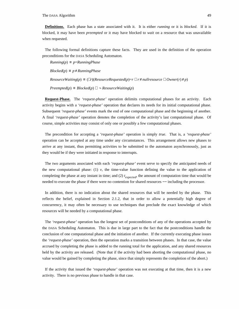
The DASA Algorithm 49
Definitions. Each phase has a state associated with it. It is either running or it is blocked. If it is
blocked, it may have been preempted or it may have blocked to wait on a resource that was unavailable
when requested.
The following formal definitions capture these facts. They are used in the definition of the operation
preconditions for the DASA Scheduling Automaton.
Running(p) ≡ p=RunningPhase
Blocked(p) ≡ p ≠ RunningPhase
ResourceWaiting(p) ≡ (∃r)(ResourceRequested(p)=r ∧ r ≠ nullresource ∧ Owner(r) ≠ p)
Preempted(p) ≡ Blocked(p) ∧ ¬ ResourceWaiting(p)
Request-Phase. The ‘request-phase’ operation delimits computational phases for an activity. Each
activity begins with a ‘request-phase’ operation that declares its needs for its initial computational phase.
Subsequent ‘request-phase’ events mark the end of one computational phase and the beginning of another.
A final ‘request-phase’ operation denotes the completion of the activity’s last computational phase. Of
course, simple activities may consist of only one or possibly a few computational phases.
The precondition for accepting a ‘request-phase’ operation is simply true. That is, a ‘request-phase’
operation can be accepted at any time under any circumstances. This arrangement allows new phases to
arrive at any instant, thus permitting activities to be submitted to the automaton asynchronously, just as
they would be if they were initiated in response to interrupts.
The two arguments associated with each ‘request-phase’ event serve to specify the anticipated needs of
the new computational phase: (1) v, the time-value function defining the value to the application of
completing the phase at any instant in time; and (2) t , the amount of computation time that would beexpected
needed to execute the phase if there were no contention for shared resources −− including the processor.
In addition, there is no indication about the shared resources that will be needed by the phase. This
reflects the belief, explained in Section 2.1.2, that in order to allow a potentially high degree of
concurrency, it may often be necessary to use techniques that preclude the exact knowledge of which
resources will be needed by a computational phase.
The ‘request-phase’ operation has the longest set of postconditions of any of the operations accepted by
the DASA Scheduling Automaton. This is due in large part to the fact that the postconditions handle the
conclusion of one computational phase and the initiation of another. If the currently executing phase issues
the ‘request-phase’ operation, then the operation marks a transition between phases. In that case, the value
accrued by completing the phase is added to the running total for the application, and any shared resources
held by the activity are released. (Note that if the activity had been aborting the computational phase, no
value would be gained by completing the phase, since that simply represents the completion of the abort.)
If the activity that issued the ‘request-phase’ operation was not executing at that time, then it is a new
activity. There is no previous phase to handle in that case.
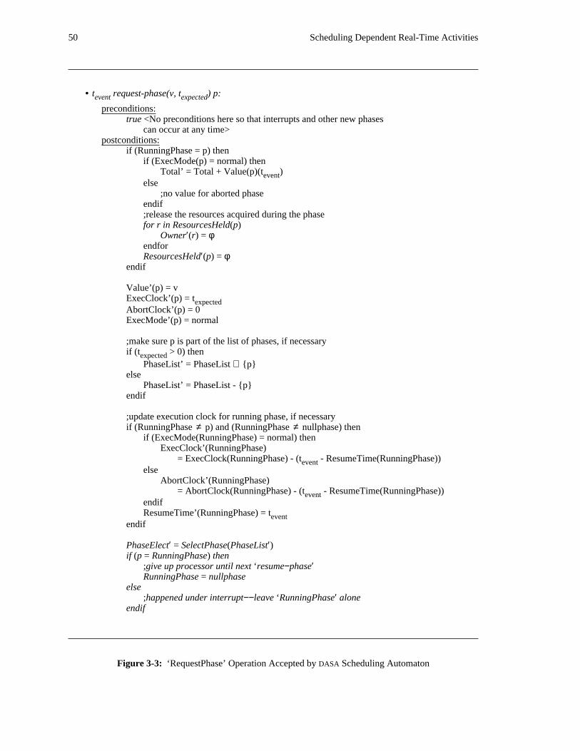
50 Scheduling Dependent Real-Time Activities
• t request-phase(v, t ) p:event expected
preconditions:true <No preconditions here so that interrupts and other new phases
can occur at any time>postconditions:
if (RunningPhase = p) thenif (ExecMode(p) = normal) then
Total’ = Total + Value(p)(t )eventelse
;no value for aborted phaseendif;release the resources acquired during the phasefor r in ResourcesHeld(p)
Owner′(r) = φendforResourcesHeld′(p) = φ
endif
Value’(p) = vExecClock’(p) = texpectedAbortClock’(p) = 0ExecMode’(p) = normal
;make sure p is part of the list of phases, if necessaryif (t > 0) thenexpected
PhaseList’ = PhaseList ∪ {p}else
PhaseList’ = PhaseList - {p}endif
;update execution clock for running phase, if necessaryif (RunningPhase ≠ p) and (RunningPhase ≠ nullphase) then
if (ExecMode(RunningPhase) = normal) thenExecClock’(RunningPhase)
= ExecClock(RunningPhase) - (t - ResumeTime(RunningPhase))eventelse
AbortClock’(RunningPhase)= AbortClock(RunningPhase) - (t - ResumeTime(RunningPhase))event
endifResumeTime’(RunningPhase) = tevent
endif
PhaseElect′ = SelectPhase(PhaseList′)if (p = RunningPhase) then
;give up processor until next ‘resume−phase′RunningPhase = nullphase
else;happened under interrupt−−leave ‘RunningPhase′ alone
endif
Figure 3-3: ‘RequestPhase’ Operation Accepted by DASA Scheduling Automaton
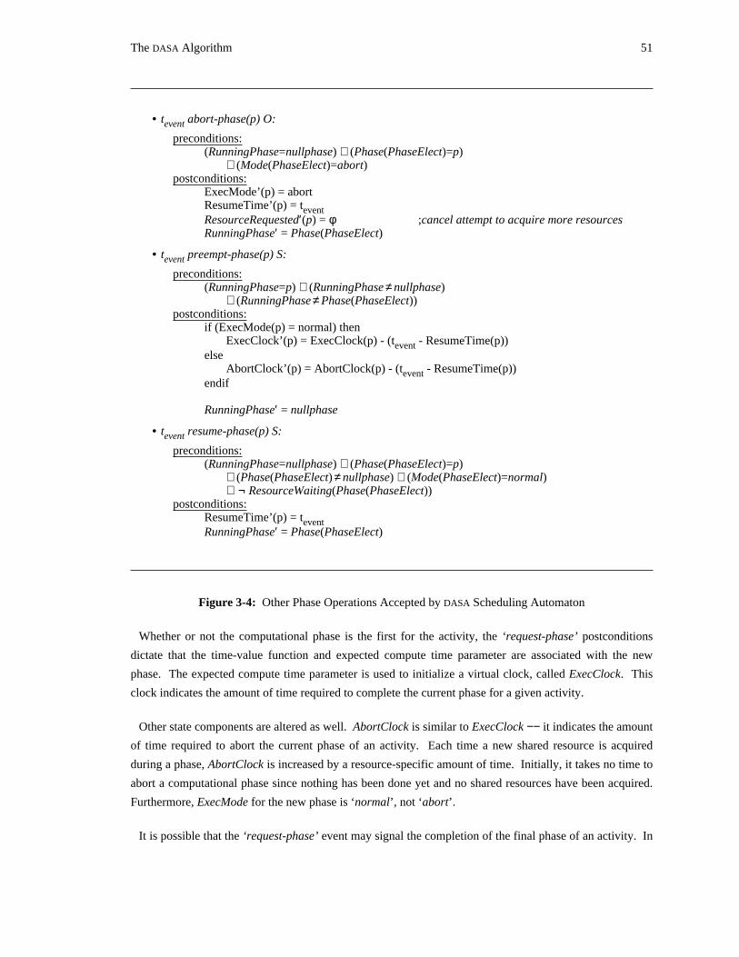
The DASA Algorithm 51
• t abort-phase(p) O:event
preconditions:(RunningPhase=nullphase) ∧ (Phase(PhaseElect)=p)
∧ (Mode(PhaseElect)=abort)postconditions:
ExecMode’(p) = abortResumeTime’(p) = teventResourceRequested′(p) = φ ;cancel attempt to acquire more resourcesRunningPhase′ = Phase(PhaseElect)
• t preempt-phase(p) S:event
preconditions:(RunningPhase=p) ∧ (RunningPhase ≠ nullphase)
∧ (RunningPhase ≠ Phase(PhaseElect))postconditions:
if (ExecMode(p) = normal) thenExecClock’(p) = ExecClock(p) - (t - ResumeTime(p))event
elseAbortClock’(p) = AbortClock(p) - (t - ResumeTime(p))event
endif
RunningPhase′ = nullphase
• t resume-phase(p) S:event
preconditions:(RunningPhase=nullphase) ∧ (Phase(PhaseElect)=p)
∧ (Phase(PhaseElect) ≠ nullphase) ∧ (Mode(PhaseElect)=normal)∧ ¬ ResourceWaiting(Phase(PhaseElect))
postconditions:ResumeTime’(p) = teventRunningPhase′ = Phase(PhaseElect)
Figure 3-4: Other Phase Operations Accepted by DASA Scheduling Automaton
Whether or not the computational phase is the first for the activity, the ‘request-phase’ postconditions
dictate that the time-value function and expected compute time parameter are associated with the new
phase. The expected compute time parameter is used to initialize a virtual clock, called ExecClock. This
clock indicates the amount of time required to complete the current phase for a given activity.
Other state components are altered as well. AbortClock is similar to ExecClock −− it indicates the amount
of time required to abort the current phase of an activity. Each time a new shared resource is acquired
during a phase, AbortClock is increased by a resource-specific amount of time. Initially, it takes no time to
abort a computational phase since nothing has been done yet and no shared resources have been acquired.
Furthermore, ExecMode for the new phase is ‘normal’, not ‘abort’.
It is possible that the ‘request-phase’ event may signal the completion of the final phase of an activity. In
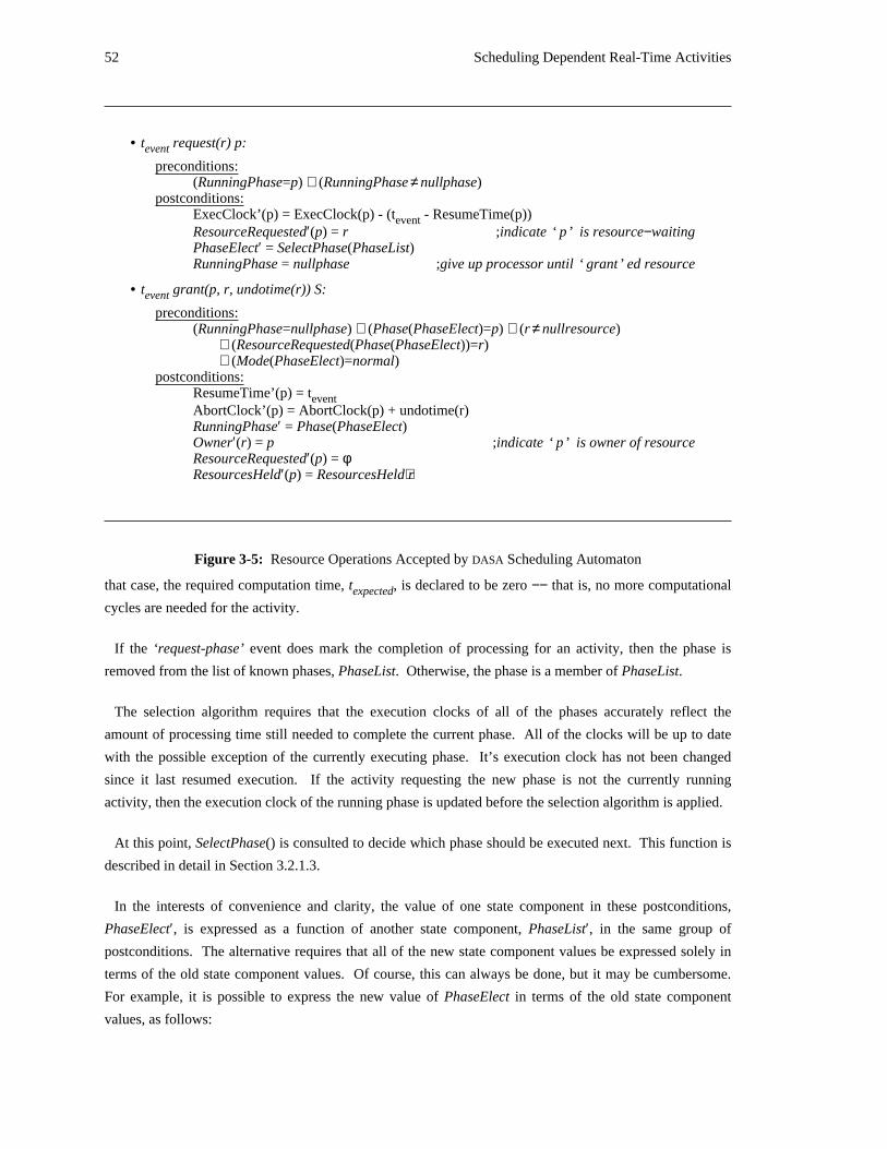
52 Scheduling Dependent Real-Time Activities
• t request(r) p:event
preconditions:(RunningPhase=p) ∧ (RunningPhase ≠ nullphase)
postconditions:ExecClock’(p) = ExecClock(p) - (t - ResumeTime(p))eventResourceRequested′(p) = r ;indicate ‘ p ’ is resource−waitingPhaseElect′ = SelectPhase(PhaseList)RunningPhase = nullphase ;give up processor until ‘ grant ’ ed resource
• t grant(p, r, undotime(r)) S:event
preconditions:(RunningPhase=nullphase) ∧ (Phase(PhaseElect)=p) ∧ (r ≠ nullresource)
∧ (ResourceRequested(Phase(PhaseElect))=r)∧ (Mode(PhaseElect)=normal)
postconditions:ResumeTime’(p) = teventAbortClock’(p) = AbortClock(p) + undotime(r)RunningPhase′ = Phase(PhaseElect)Owner′(r) = p ;indicate ‘ p ’ is owner of resourceResourceRequested′(p) = φResourcesHeld′(p) = ResourcesHeld⋅r
Figure 3-5: Resource Operations Accepted by DASA Scheduling Automaton
that case, the required computation time, t , is declared to be zero −− that is, no more computationalexpected
cycles are needed for the activity.
If the ‘request-phase’ event does mark the completion of processing for an activity, then the phase is
removed from the list of known phases, PhaseList. Otherwise, the phase is a member of PhaseList.
The selection algorithm requires that the execution clocks of all of the phases accurately reflect the
amount of processing time still needed to complete the current phase. All of the clocks will be up to date
with the possible exception of the currently executing phase. It’s execution clock has not been changed
since it last resumed execution. If the activity requesting the new phase is not the currently running
activity, then the execution clock of the running phase is updated before the selection algorithm is applied.
At this point, SelectPhase() is consulted to decide which phase should be executed next. This function is
described in detail in Section 3.2.1.3.
In the interests of convenience and clarity, the value of one state component in these postconditions,
PhaseElect′, is expressed as a function of another state component, PhaseList′, in the same group of
postconditions. The alternative requires that all of the new state component values be expressed solely in
terms of the old state component values. Of course, this can always be done, but it may be cumbersome.
For example, it is possible to express the new value of PhaseElect in terms of the old state component
values, as follows:
The DASA Algorithm 53
if (t > 0) thenexpectedPhaseElect′ = SelectPhase(PhaseList ∪ {p})
elsePhaseElect′ = SelectPhase(PhaseList − {p})
endif
Finally, if the currently executing activity, RunningPhase, issued the ‘request-phase’ event, it surrenders
the processor −− clearing the way to execute the PhaseElect specified by SelectPhase().
Note that surrendering the processor really has no effect if PhaseElect specifies that the currently
executing activity should continue. In that case, while the processor will nominally begin executing the
nullphase, it will actually resume execution of the PhaseElect immediately. The transition to the nullphase
is only a convenience in terms of modeling the automaton. After reviewing the other scheduling events
accepted by the DASA Scheduling Automaton, the convention employed throughout to mark potential
changes in execution due to a preemption, abortion, or unsatisfiable request should be clear.
Abort-Phase. As modeled, phases are aborted only as a result of a decision by the scheduling function,26SelectPhase() .
By convention, each time the executing activity, RunningPhase, makes a new request to either begin a
new phase or to acquire a new shared resource −− necessitating a scheduling decision −− the activity gives
up the processor. That is, as a postcondition for accepting one of these requests, RunningPhase is set to be
nullphase. This is done to meet the preconditions to accept either an ‘abort-phase’ or a ‘resume-phase’
event. Once the processor is idle, then if the execution mode of PhaseElect is ‘abort’, then an
‘abort-phase’ event can be accepted by the DASA Scheduling Automaton.
The postconditions for this event make sure that the phase is aborting, note the time at which execution
resumed, cancel any outstanding requests for shared resources (since no new resources must be acquired to
undo whatever was done to those previously acquired), and designate the new executing phase.
Preempt-Phase. As indicated by its precondition, the scheduler issues a ‘preempt-phase’ event if the
processor is executing some phase other than the PhaseElect or the nullphase. In response, the current
RunningPhase is suspended, its execution clock (either ExecClock or AbortClock, depending on the
execution mode) is updated to reflect the true time left to free the shared resources held by the phase, and
the processor is left idle.
Of course, the processor will probably not remain idle for long since either an ‘abort-phase’, a
‘resume-phase’, or a ‘grant’ event will be issued to execute another phase: (1) an ‘abort-phase’ event is
issued for a phase that is being aborted; (2) a ‘resume-phase’ event is issued for a phase that is executing
26This should not be viewed as precluding the possibility of an activity aborting a phase autonomously −− perhaps due to a failurewithin a transaction. Rather, the model can easily be extended to accommodate that possibility: If the executing activity decides toabort the current phase, it issues an ‘abort-self’ event. This event changes the execution mode of the phase to ‘abort’, consultsSelectPhase() to determine what to run next, and gives up the processor. When the scheduler selected that phase to begin its abortprocessing, it would issue an ‘abort-phase’ event, and processing would continue as described above.
54 Scheduling Dependent Real-Time Activities
normally, but is not waiting for a resource (that is, it is a previously preempted phase); and (3) a ‘grant’
event is issued for a phase that is executing normally and is waiting for access to a shared resource. All
three of these scheduling events require that the processor be idle before they dispatch the next phase.
(Along with the ‘preempt-phase’ event, the ‘request-phase’ and ‘request’ events also leave the processor
idle when appropriate to set the stage for these phase-dispatching events.)
Resume-Phase. The ‘resume-phase’ event resumes the execution of a previously preempted phase. The
processor must be idle before a ‘resume-phase’ event can be accepted by the DASA Scheduling Automaton,
and the phase resumed must be executing normally −− as opposed to aborting −− and must not be waiting
on access to a shared resource.
The postconditions for the acceptance of a ‘resume-phase’ event note the time at which execution of the
phase resumed and assign the processor to execute the phase.
Request. A ‘request’ event signals that the currently executing phase wishes to access a shared resource.
As denoted by the event’s preconditions, such a request can be made at any time while the phase is
executing on the processor.
After accepting a ‘request’ event, the postconditions for the event update the requesting phase’s execution
clock to indicate the exact time left to complete the phase, record the resource that has been requested by
the phase, select the next phase to be executed (possibly the requesting phase), and remove the requesting
phase from the processor.
It should be understood that the decision to suspend the requesting phase’s execution is only made to
provide a simple, coherent formal model, not to suggest the actual design of an implementation of the DASA
algorithm. Notice, for example, that in the formal model, it is quite possible that a phase could request a
resource that is currently available, give up the processor, and immediately be reassigned the processor as
the result of a ‘grant’ event. This is perfectly fine in the model, but an efficient implementation of the
algorithm should decide whether the processor should actually be turned over to another phase before ever
suspending execution of the current phase.
Grant. The ‘grant’ scheduling event assigns the processor, which must be idle, to execute a phase that
has been blocked awaiting access to a shared resource. The phase assigned to execute has been previously
selected and is designated PhaseElect.
Once the ‘grant’ event has been accepted by the DASA Scheduling Automaton, the postconditions
associated with that event record the time at which the phase is granted the resource, adjusts the AbortClock
to indicate the increment in work that is required to undo actions on the newly acquired shared resource,
manipulates various relations to show that the resource now belongs to the designated phase, and starts the
processor executing that phase.
Although there are ‘request’ and ‘grant’ events, there is no explicit ‘release’ event. This is due to the
model of computation that has been adopted. Since all activities are composed of a sequence of
The DASA Algorithm 55
computational phases and all shared resources that are acquired during a phase are released at the
completion of the phase, there is no need for such an event. Rather, an implicit release of these resources is
performed as part of the ‘request-phase’ event, which, among other things, denotes the completion of a
phase (as described above).
3.2.1.3. SelectPhase() Function for DASA Automaton
The function SelectPhase() embodies the DASA scheduling algorithm. As shown in Section 3.2.1.2,
SelectPhase() is evaluated each time a ‘request-phase’ or a ‘request’ event is encountered. In Figure 3-6,
SelectPhase() is formally defined as a mathematical function. Since this definition looks quite different
than the brief procedural definition offered in Section 3.1.2.1, a few comments are in order to explain the
utility of this format and its organization.
The algorithm is described as a mathematical function for a few reasons. First and foremost, it is a
concise and precise notation. But it also is more expressive in some ways than procedural definitions.
Specifically, this mathematical format is capable of expressing the sequential nature of a set of operations
−− by using functional composition, for example, where each function corresponds to one of the sequential
operations. At the same time, this mathematical format can also express the nondeterminism that is present
in the algorithm definition. For instance, the order in which the elements in a list are examined may or may
not be important. When the order is important, there is a specific method to describe the order. This is said
to be deterministic, in that there is only one correct order. When the order is unimportant, any order will
do; and so this case is said to be nondeterministic. A typical procedural definition cannot readily capture
this nondeterminism. Such a definition would usually have to specify some ordering, even if the ordering
was not critical.
The function SelectPhase(), when given a list of phases, selects the next phase to run and specifies its
execution mode (either ‘normal’ or ‘abort’). Informally, the definition shown for SelectPhase() in Figure
3-6 determines a set of phases that can feasibly meet their time constraints given all of the information that
is currently known about them. It then selects one of the phases from this set that must be done by the
earliest deadline and designates it as the next phase that the processor should execute.
All of the phases in the phase list P that was passed to SelectPhase() are considered when constructing the
list of phases that can feasibly execute. Also, as each phase is examined in turn, any dependency that
prevents it from executing immediately are noted and resolved by indicating those other activities that must
precede it in any schedule −− either completing or aborting their current phases.
A closer look is necessary to see how the SelectPhase() definition actually specifies the desired behavior.
A bottom-up examination of the definition will incorporate both some functions that have been discussed
previously and some totally new functions.
The following descriptions constitute an informal definition of the functions comprising SelectPhase().
Often only the "main" or "normal" case value will be discussed for a function, even though its definition
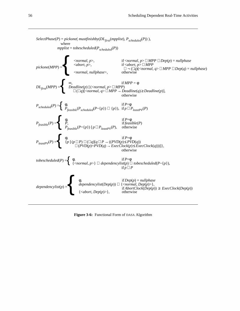
56 Scheduling Dependent Real-Time Activities
SelectPhase(P) = pickone( mustfinishby(DL (mpplist), P (P)) ),first scheduledwhere
mpplist = tobescheduled(P (P))scheduled
<normal, p>, if <normal, p> ∈ MPP ∧ Dep(p) = nullphase<abort, p>, if <abort, p> ∈ MPP
pickone(MPP) = ∧ ¬ (∃q)(<normal, q> ∈ MPP ∧ Dep(q) = nullphase){<normal, nullphase>, otherwise
∞, if MPP = φDL (MPP) = Deadline(p) | (<normal, p> ∈ MPP)first { ∧ (∀q)[<normal, q> ∈ MPP → Deadline(q) ≥ Deadline(p)],
otherwise
φ, if P=φP (P) =scheduled { P (P (P−{p}) ∪ {p}), if p ∈ P (P)feasible scheduled leastPV
φ, if P=φP (P) = P, if feasible(P)feasible { P (P−{p}) | p ∈ P (P), otherwisefeasible leastPV
φ, if P=φP (P) = {p | (p ∈ P) ∧ (∀q)[q ∈ P → ((PVD(p) ≤ PVD(q))leastPV { ∧ (PVD(p)=PVD(q) → ExecClock(p) ≤ ExecClock(q)))]},
otherwise
φ, if P=φtobescheduled(P) ={ {<normal, p>} ∪ dependencylist(p) ∪ tobescheduled(P−{p}),if p ∈ P
φ, if Dep(p) = nullphasedependencylist(Dep(p)) ∪ {<normal, Dep(p)>},
dependencylist(p) = if AbortClock(Dep(p)) ≥ ExecClock(Dep(p)){{<abort, Dep(p)>}, otherwise
Figure 3-6: Functional Form of DASA Algorithm
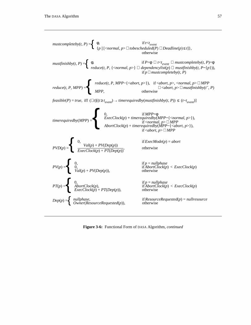
The DASA Algorithm 57
φ, if t<tmustcompleteby(t, P) = event{{p | [<normal, p> ∈ tobescheduled(P) ∧ Deadline(p) ≤ t]},
otherwise
φ, if P=φ ∨ t<t ∨ mustcompleteby(t, P)=φmustfinishby(t, P) = event{reduce(t, P, {<normal, p>} ∪ dependencylist(p) ∪ mustfinishby(t, P−{p})),
if p ∈ mustcompleteby(t, P)
reduce(t, P, MPP−{<abort, p>}), if <abort, p>, <normal, p> ∈ MPP−reduce(t, P, MPP) = ∧ <abort, p> ∉ mustfinishby(t , P){ MPP, otherwise
feasible(P) = true, iff (∀t)[(t ≥ t ) → timerequiredby(mustfinishby(t, P)) ≤ (t−t )]event event
0, if MPP=φExecClock(p) + timerequiredby(MPP−{<normal, p>}),
timerequiredby(MPP) = if <normal, p> ∈ MPP{AbortClock(p) + timerequiredby(MPP−{<abort, p>}),
if <abort, p> ∈ MPP
0, if ExecMode(p) = abortVal(p) + PV(Dep(p))
PVD(p) ={ , otherwiseExecClock(p) + PT(Dep(p))
0, if p = nullphasePV(p) = 0, if AbortClock(p) < ExecClock(p){ Val(p) + PV(Dep(p)), otherwise
0, if p = nullphasePT(p) = AbortClock(p), if AbortClock(p) < ExecClock(p){ ExecClock(p) + PT(Dep(p)), otherwise
nullphase, if ResourceRequested(p) = nullresourceDep(p) ={ Owner(ResourceRequested(p)), otherwise
Figure 3-6: Functional Form of DASA Algorithm, continued
58 Scheduling Dependent Real-Time Activities
27includes a number of other cases as well . This is because the other cases usually handle degenerate
situations that arise as a result of the recursive nature of some of the function definitions.
To start, remember that a few basic functions were described in Section 2.3.1. They include Deadline()
and Val() and are used in the definitions that follow as basic building blocks.
Also remember that SelectPhase() is a function that is evaluated within the context of the DASA
scheduling automaton. As such, it has access to all of the state components of the automaton, which in turn
provides access to all of the status information for each phase in the system. Furthermore, since
SelectPhase() is always evaluated as a result of accepting a scheduling operation, the t that appears inevent
the formal definition refers to the timestamp for the accepted event.
One shorthand notation with regard to the state components has been adopted in the function definitions:
whenever SelectPhase() is evaluated, it accesses the state component values that result from the
postconditions for the event being accepted. For instance, when a ‘request-phase’ event is accepted,
SelectPhase() accesses ExecClock′(p), rather than ExecClock(p). This permits a more convenient
presentation of the functions than would be possible if additional cases had to be added to the functions
solely to produce the postcondition value for each relevant state component instead of referencing it
directly. The outcome is the same in both cases.
With that background in mind, we can begin to examine the formal definition of SelectPhase() in earnest.
Consider first the set of functions that form the dependency lists and evaluate the potential value densities
of all of the phases in the system.
The function ‘Dep()’, evaluated for a specified phase, returns as its value the phase that is currently
preventing the specified phase from executing (due to a dependency). If the phase is ready to execute
immediately, then the ‘nullphase′ is the value of ‘Dep()’. Otherwise, the phase has requested a shared
resource and is dependent on the owner of that resource −− that is the phase that currently holds the shared
resource −− if there is one. The phase holding the resource must relinquish it before the dependent phase
can continue execution.
The resource can be relinquished in one of two ways: either the phase can complete its normal course of28execution or it can be aborted. Both of these alternatives take time , and the DASA algorithm attempts to
minimize the amount of time waiting for the resource. So DASA completes the phase unless it is faster to
abort it.
The function ‘dependencylist()’ uses the information supplied by ‘Dep()’ about the dependencies of
27Which case is to be used to evaluate the function typically depends on the value of one or more arguments to the function.
28As was pointed out in Section 2.1.4, a phase that has been aborted does not instantaneously return the shared resources allocatedto it to the system. Rather, the shared resources must be placed into a meaningful, acceptable, safe, and (possibly) consistent, stateprior to their release. It is the processing that puts the shared resources into these acceptable states that consumes time after an aborthas been issued for the phase.
The DASA Algorithm 59
individual phases to construct a list that includes all of the phases that must execute before a specified
phase. ‘Dependencylist()’ also specifies the execution mode for each of the phases that must be executed
prior to the specified phase. Therefore, the dependency list is actually a set of mode-phase pairs of the
form <mode, phase>. It is in this function that the decision to minimize the length of time to remove
dependencies is implemented.
The definition of the function is recursive. It initially examines the phase, p, that was given as its
argument. If p is not dependent on any other phase, then its dependency list is empty. Otherwise, it will be
non-empty. Specifically, if it is faster to abort the phase on which p depends, then the dependency list will
have only one member: <abort, Dep(p)>. Alternatively, if it is at least as fast to complete the normal
execution of the phase on which p depends, then p’s dependency list will be constructed by adding
<normal, Dep(p)> to the dependency list of Dep(p).
Once a dependency list has been determined for a phase, it is possible to evaluate the potential value
density for that phase. This is done by the function PVD(), which employs two auxiliary functions, PV()
and PT(). These functions are similar to those discussed earlier in this chapter, in Section 3.1.2.1. They
total the value that may be accrued and the execution time that is required jointly by the given phase and all
of the phases in its dependency list. (Note that aborting a phase requires time but yields no value directly.)
These totals are then used to determine the potential value density for the specified phase.
The function P () examines a set of phases and returns the subset of phases that have the lowestleastPV
potential value. In case more than one phase has the same (lowest) potential value density, the phase or
phases that will consume the least execution time is returned. This choice is made because, when
considering two phases with the same PVD, the phase that executes longer will obtain a higher value than
the one that runs shorter since value is the product of PVD and execution time.
Another group of functions determine the amount of time required to carry out a specified set of
executions and aborts over all of the critical time intervals, thereby allowing the feasibility of the specified
computations to be ascertained. So, for instance:
• tobescheduled() −− given a set of phases to be executed, this function determines the set ofmode-phase pairs that must be scheduled in order to eliminate existing dependencies involvingthat set of phases; this set of mode-phase pairs includes each of the phases in the specified setexecuting in normal mode;
• timerequiredby() −− given a set of mode-phase pairs, this function determines the totalexecution time required to carry out all of the specified computations;
• mustcompleteby() −− given a time and a set of phases, this function identifies those phases thatmust complete execution by the specified time;
• mustfinishby() −− given a time and a set of phases, this function identifies all of the normalexecutions and abortions that must finish by the specified time; whereas, mustcompleteby()identified those phases that had to complete their normal executions by the specified time,mustfinishby() adds to that group all of the other work that must be done in order to removeany existing dependencies that might prevent those phases from executing immediately; alsonotice that this function uses another function, reduce(), to eliminate unnecessary aborts fromthe resultant list;
• reduce() −− this function eliminates unnecessary aborts by noticing cases where the same
60 Scheduling Dependent Real-Time Activities
29phase is being both completed and aborted , but the completion must be done prior to theabort due to the dependencies currently in effect; of course, there is no need to abort a phaseonce it has completed;
• feasible() −− given a set of phases, this function determines whether all of the phases in the set,along with all of the other computations on which they depend, can meet their deadlines; for aschedule to be feasible, at every point in time the total amount of time required to complete thecomputations that must be done by that time must never exceed the actual time remaining untilthat time.
With this set of functions to use as building blocks, it is possible to describe at a fairly high level how to
select the phase that should execute next.
A set of phases that can be feasibly run (given current knowledge of requirements and resources) is
constructed by examining each existing phase ordered by PVD, starting with the phase with the highest30PVD. The functions P () and P () construct this set . Given a set of N phases, P ()scheduled feasible scheduled
will first (recursively) determine which of the N−1 phases with the greatest potential value may feasibly be
executed. P (), using P () and ultimately feasible(), then determines if the phase with the leastscheduled feasible
potential value can feasibly be added to the set. If so, it is.
Once P () has identified which phases can be completed successfully, it is fairly straightforward toscheduled
determine which phase should be executed first. The auxiliary function DL () specifies the earliestfirst
deadline that must be met by those phases that can complete execution. That information, along with the
set of phases to be completed, is once again passed to the function mustfinishby() to determine all of the
work that must be done by the earliest deadline. And finally, pickone() selects a mode-phase pair from that
set to execute first. pickone() always prefers to complete a phase normally if possible, but if that cannot be
done, it will initiate (or continue) the abortion of a phase.
3.2.2. Observations on the Definition
Several observations can be made now that the formal definition of the DASA Scheduling Automaton has
been presented in full. Each of the following sections focus on an interesting observation.
3.2.2.1. Manifestation of Desirable Properties
Section 3.1.1 listed five desirable properties that the DASA algorithm should possess. Now that the
algorithm has been presented in some depth, those properties should be reviewed again:1. explicitly account for dependencies −− this has been accomplished. The definition of
SelectPhase() was described from the bottom up, and the first thing that was done inconsidering any phase was to determine those phases that it depends on (its dependency list)and the aggregate value of this group of phases to the application.
29It is not unexpected that both the completion and the abortion of a single phase will sometimes be executed. In the expected case,the phase is aborted in order to allow some other phase, with a tighter deadline, to execute. Later, the aborted phase can be restartedand completed normally, still meeting its time constraint.
30Note that the functions that are named P () all represent sets of phases.x
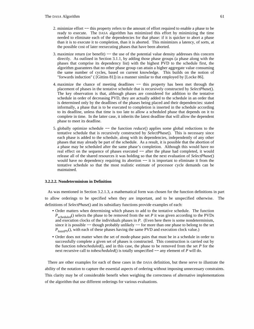
The DASA Algorithm 61
2. minimize effort −− this property refers to the amount of effort required to enable a phase to beready to execute. The DASA algorithm has minimized this effort by minimizing the timeneeded to eliminate each of the dependencies for that phase: if it is quicker to abort a phasethan it is to execute it to completion, than it is aborted. This minimizes a latency, of sorts, atthe possible cost of later reexecuting phases that have been aborted.
3. maximize return (or benefit) −− the use of the potential value density addresses this concerndirectly. As outlined in Section 3.1.1, by adding those phase groups (a phase along with thephases that comprise its dependency list) with the highest PVD to the schedule first, thealgorithm guarantees that no other phase group can attain a higher aggregate value consumingthe same number of cycles, based on current knowledge. This builds on the notion of"forwards induction" ( [Gittins 81]) in a manner similar to that employed by [Locke 86].
4. maximize the chance of meeting deadlines −− this property has been met through theplacement of phases in the tentative schedule that is recursively constructed by SelectPhase().The key observation is that, although phases are considered for addition to the tentativeschedule in order of decreasing PVD, they are actually added to the schedule in an order thatis determined only by the deadlines of the phases being placed and their dependencies: statedinformally, a phase that is to be executed to completion is inserted in the schedule accordingto its deadline, unless that time is too late to allow a scheduled phase that depends on it tocomplete in time. In the latter case, it inherits the latest deadline that will allow the dependentphase to meet its deadline.
5. globally optimize schedule −− the function reduce() applies some global reductions to thetentative schedule that is recursively constructed by SelectPhase(). This is necessary sinceeach phase is added to the schedule, along with its dependencies, independently of any otherphases that may already be part of the schedule. As a result, it is possible that the abortion ofa phase may be scheduled after the same phase’s completion. Although this would have noreal effect on the sequence of phases executed −− after the phase had completed, it wouldrelease all of the shared resources it was holding so that the next evaluation of SelectPhase()would have no dependency requiring its abortion −− it is important to eliminate it from thetentative schedule so that the most realistic estimate of processor cycle demands can bemaintained.
3.2.2.2. Nondeterminism in Definition
As was mentioned in Section 3.2.1.3, a mathematical form was chosen for the function definitions in part
to allow orderings to be specified when they are important, and to be unspecified otherwise. The
definitions of SelectPhase() and its subsidiary functions provide examples of each:
• Order matters when determining which phases to add to the tentative schedule. The functionP () selects the phase to be removed from the set P it was given according to the PVDsscheduledand execution clocks of the individuals phases in P. (Even here there is some nondeterminism,since it is possible −− though probably unlikely −− for more than one phase to belong to the setP (), with each of these phases having the same PVD and execution clock value.)leastPV
• Order does not matter when the set of mode-phase pairs that must be in a schedule in order tosuccessfully complete a given set of phases is constructed. This construction is carried out bythe function tobescheduled(), and in this case, the phase to be removed from the set P for thenext recursive call to tobescheduled() is totally unspecified −− any element of P will do.
There are other examples for each of these cases in the DASA definition, but these serve to illustrate the
ability of the notation to capture the essential aspects of ordering without imposing unnecessary constraints.
This clarity may be of considerable benefit when weighing the correctness of alternative implementations
of the algorithm that use different orderings for various evaluations.
62 Scheduling Dependent Real-Time Activities
3.2.2.3. Explicit Appearance of Time
Time does not explicitly appear in many of the individual function definitions. This may be unexpected
for an environment where time −− and meeting time constraints −− is a central concern. Of necessity, time
explicitly plays a role in testing the feasibility of executing groups of phases. And while this testing occurs
throughout the evaluation of SelectPhase(), references to time seem infrequent since phases are added to
the tentative schedule according to their potential value density, not according to the urgency of their time
constraints.
3.3. Scheduling Example Revisited
Now that the scheduling algorithm has been presented, it is possible to reconsider the scheduling example
discussed in Section 1.3. Once again, the problem is to schedule phases p , p , and p so as to meet theira b c
time constraints, if possible. In fact, it is possible, and this is shown by the bottom execution profile in
Figure 3-7. Notice that phase p is aborted during the course of execution, thus allowing phase p to meeta b
its deadline. This necessitates the reexecution of the start of phase p at a later time.a
The top of Figure 3-7 shows the execution profile for a scheduler that is identical to DASA, except that it
cannot abort phases. It, too, meets all of the deadlines, while consuming fewer cycles than DASA in the
process. However, it must tolerate a longer delay between the time that it determines that a given phase
should be executed and the time at which that phase may actually begin execution due to existing
dependencies. This variant of the DASA algorithm is shown only as a reference point. At this point, it is not
anticipated that it will studied in significant depth as part of the proposed thesis research.
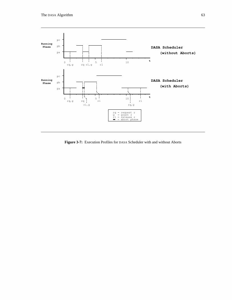
The DASA Algorithm 63
= abort phase
rl
rq,g
rq,g
rl
rl
rl,g
rq
rl,g
(without Aborts)
DASA Scheduler
DASA Scheduler
(with Aborts)
RunningPhase
PhaseRunning
t5 100
0 105
pa
pb
pc
pc
pb
pa
t
rq,g rq
rq = request rg = grant rrl = release r
Figure 3-7: Execution Profiles for DASA Scheduler with and without Aborts

64 Scheduling Dependent Real-Time Activities
Chapter 4
Analytic Results
This chapter presents a set of analytic results that argue for the benefits of the DASA algorithm. First, a
number of high-level requirements that real-time scheduling algorithms must possess is discussed. Then a
strategy for demonstrating that the DASA scheduling algorithm possess those properties is outlined,
followed by a set of proofs conforming to that strategy. The final section of the chapter discusses various
interesting behaviors that the DASA algorithm may demonstrate, which are revealed by its formal
description.
4.1. Requirements for Scheduling Algorithms
Any practical solution to the problem of scheduling while taking dependencies into account must be
correct, valuable, and tractable.
The solution must be correct. Specifically, any scheduling decisions that are made must observe all of
the known dependencies. Therefore, for instance, any activity that is selected to execute must be able to
execute at that point in time. The solution must also obey the concurrency control rules of the model; in
particular, for the model presented here, mutually exclusive access to the shared resources must be
guaranteed.
The solution must be valuable. When cast in the computational model described above, this requirement
simply means that the schedules dictated by the scheduler must yield good values relative to other
scheduling algorithms. Notice that this is partially a comment on the scheduler’s behavior in normal
situations and partially a comment on its behavior in overload situations. In normal (non-overload)
situations, the ordering of activities is critical and many schedulers will not order them appropriately, even
when there are sufficient processor cycles present to satisfy all demands; in overload situations, the31application (and the system) should display a graceful degradation of function . Both of these types of
situation are accurately gauged by the value metric previously introduced.
Finally, the solution must be computationally tractable. In fact, it must be efficient. For the purposes of
this work, this means that the solution must consume, at worst, an amount of time and space that is
31Even schedulers that take dependencies into account may handle overload situations differently, resulting in different schedulingdecisions, and hence different values, for executing the application.
65
66 Scheduling Dependent Real-Time Activities
polynomial in the problem size −− in this case, the problem’s size is the number of phases under
consideration by the scheduler.
4.2. Strategy for Demonstrating Requirement Satisfaction
Analytic proofs have been constructed to demonstrate the correctness, value, and tractability of the DASA
algorithm. These proofs are contained in Section 4.3.
To demonstrate correctness, it is shown that the DASA algorithm respects any existing dependencies
among phases and makes legal selections. This is accomplished by demonstrating that any phase that DASA
selects for execution is capable of executing immediately. Specifically, it is shown that DASA will either
(1) select a phase that is ready to run (that is, one that is not blocked waiting for an allocated resource), or
(2) designate that a phase is to be aborted, since an abort may commence immediately for any phase. This
proof is presented in Section 4.3.1.
To demonstrate value, proofs serve to illustrate that DASA performs well when compared to other
scheduling algorithms in appropriate situations. In particular, when there are no dependency
considerations, DASA can be compared to a number of well-known algorithms. In fact, it is shown that, if
there are no overload conditions, the DASA automaton will accept the same histories as an automaton that
accepts histories conforming to Locke’s Best Effort Scheduling Algorithm (LBESA). Not coincidentally,
this is simply a deadline-ordered history. In overload situations, it is demonstrated that the DASA
automaton will accept histories that the LBESA automaton will not accept, and that these histories may have
a higher value than any history that the LBESA automaton may accept involving the same phases with the
same scheduling parameters. These proofs are presented in Section 4.3.2.
To demonstrate tractability, a procedural version of the DASA algorithm has been developed, and its
computational complexity has been analyzed to prove that the time and space requirements of the algorithm
are indeed polynomial in problem size −− that is, that the time and space required to execute the algorithm
are each proportional to the number of active phases raised to some constant power. Both the procedural
version of the DASA algorithm and the derivation of its space and time properties are presented in Section
4.3.3.
4.3. Proofs of Properties
The proofs in the sections that follow demonstrate properties of the DASA scheduling algorithm according
to the strategy outlined in the preceding section. Each section contains all of the proofs corresponding to a
single property of concern. In addition to the proofs themselves, other material that must be developed to
complete the proofs is also presented. For example, in Section 4.3.2.1, a derivation of another scheduling
automaton is presented. This automaton is subsequently used in proofs to assess the utility of the DASA
algorithm.
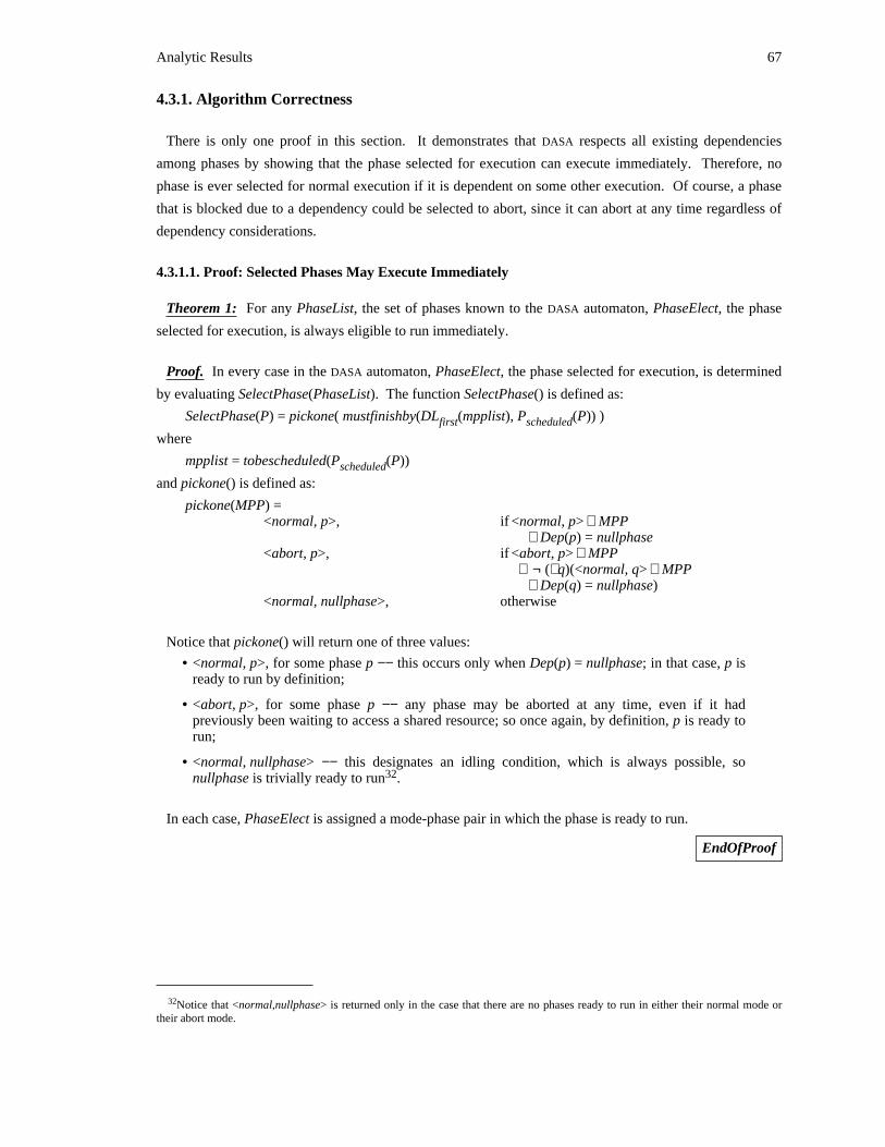
Analytic Results 67
4.3.1. Algorithm Correctness
There is only one proof in this section. It demonstrates that DASA respects all existing dependencies
among phases by showing that the phase selected for execution can execute immediately. Therefore, no
phase is ever selected for normal execution if it is dependent on some other execution. Of course, a phase
that is blocked due to a dependency could be selected to abort, since it can abort at any time regardless of
dependency considerations.
4.3.1.1. Proof: Selected Phases May Execute Immediately
Theorem 1: For any PhaseList, the set of phases known to the DASA automaton, PhaseElect, the phase
selected for execution, is always eligible to run immediately.
Proof. In every case in the DASA automaton, PhaseElect, the phase selected for execution, is determined
by evaluating SelectPhase(PhaseList). The function SelectPhase() is defined as:
SelectPhase(P) = pickone( mustfinishby(DL (mpplist), P (P)) )first scheduled
where
mpplist = tobescheduled(P (P))scheduled
and pickone() is defined as:
pickone(MPP) =<normal, p>, if <normal, p> ∈ MPP
∧ Dep(p) = nullphase<abort, p>, if <abort, p> ∈ MPP
∧ ¬ (∃q)(<normal, q> ∈ MPP∧ Dep(q) = nullphase)
<normal, nullphase>, otherwise
Notice that pickone() will return one of three values:
• <normal, p>, for some phase p −− this occurs only when Dep(p) = nullphase; in that case, p isready to run by definition;
• <abort, p>, for some phase p −− any phase may be aborted at any time, even if it hadpreviously been waiting to access a shared resource; so once again, by definition, p is ready torun;
• <normal, nullphase> −− this designates an idling condition, which is always possible, so32nullphase is trivially ready to run .
In each case, PhaseElect is assigned a mode-phase pair in which the phase is ready to run.
EndOfProof
32Notice that <normal,nullphase> is returned only in the case that there are no phases ready to run in either their normal mode ortheir abort mode.
68 Scheduling Dependent Real-Time Activities
4.3.2. Algorithm Value
Since most scheduling algorithms do not utilize dependency information, it is difficult to make fair
comparisons between their performance and that of DASA when dependencies are involved. Therefore, this
section will compare DASA to an another algorithm (LBESA) in the absence of any dependencies.
Since LBESA was shown in [Locke 86] to outperform a number of standard algorithms in a range of
situations, a favorable comparison with LBESA will demonstrate that DASA behaves well.
To that end, the two proofs presented in this section demonstrate that the DASA algorithm performs well
when compared to the LBESA algorithm. They consider a set of activities that are independent of one
another, each of which is described by a time-value function that is a step function. They show:1. If there is no overload, then both DASA and LBESA yield identical expected value to the
application.
2. Under overload, DASA may schedule more activities than LBESA, yielding a greater expectedvalue than LBESA.
Before presenting the two proofs, the next two sections develop the formal scheduling automata that they
will use. First, Section 4.3.2.1 presents the LBESA Scheduling Automaton. Then Section 4.3.2.2 presents a
scheduling automaton corresponding to the DASA algorithm when there are no dependencies to consider.
4.3.2.1. LBESA Scheduling Automaton
The LBESA Scheduling Automaton is cast using the General Scheduling Automaton Framework described
in Section 2.3.2. Once again, each scheduling decision is made based on the set of phases currently known
to the automaton: {p , p , p , . . . }.0 1 2
LBESA Automaton State Components. The state components associated with the LBESA Scheduling
Automaton are presented in Figure 4-1. They are simply the General State Components that every
scheduling automaton contains, and they were described in detail in Section 2.3.2.9.
Operations Accepted by LBESA Automaton. The operations accepted by the LBESA automaton and their
preconditions and postconditions are shown in Figures 4-2 and 4-3.
These are a somewhat simpler version of those presented in Section 3.2.1.2 for the DASA Scheduling
Automaton. Most notably, there are no operations for dealing with resources −− in particular, there are no
‘request’ and ‘grant’ operations. (Of course, in keeping with the General Scheduling Automaton
Framework, these operations actually exist for the LBESA Scheduling Automaton. However, their
preconditions are defined to be false, indicating that events with these operations can never be accepted by
the LBESA Scheduling Automaton.) In addition, there are no postconditions for ‘request-phase’ to release
previously acquired resources, and the precondition for ‘resume-phase’ is one term shorter.
The LBESA Scheduling Automaton does not accept ‘abort-phase’ operations either. This is because the
LBESA scheduling algorithm does not abort activities or phases. Such aborts are not required because the
activities are all assumed to be independent.
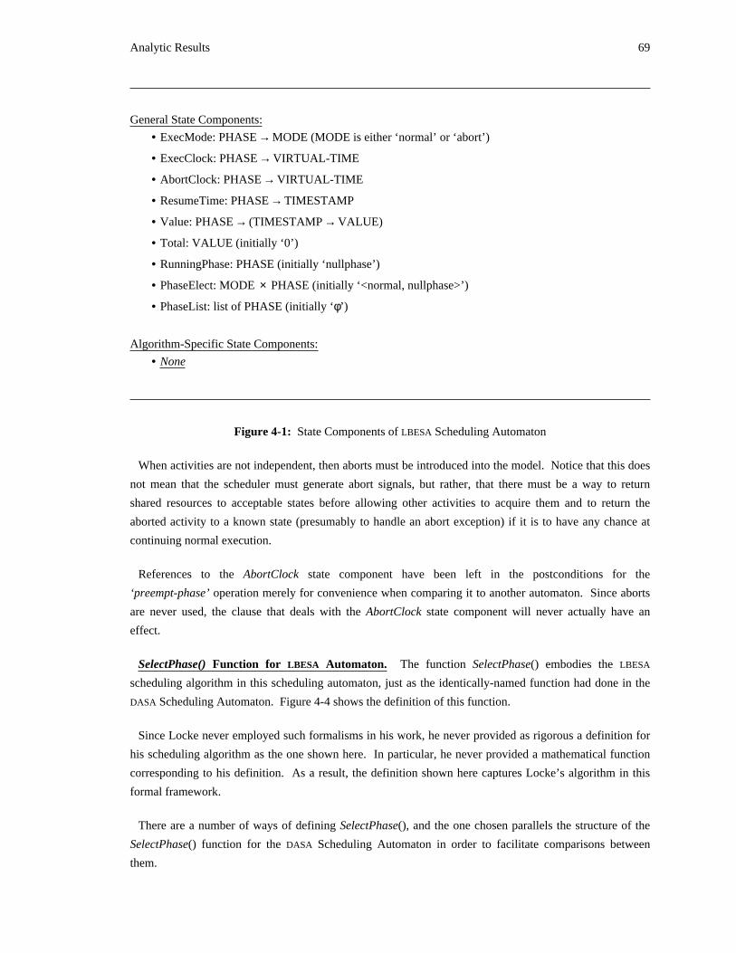
Analytic Results 69
General State Components:
• ExecMode: PHASE → MODE (MODE is either ‘normal’ or ‘abort’)
• ExecClock: PHASE → VIRTUAL-TIME
• AbortClock: PHASE → VIRTUAL-TIME
• ResumeTime: PHASE → TIMESTAMP
• Value: PHASE → (TIMESTAMP → VALUE)
• Total: VALUE (initially ‘0’)
• RunningPhase: PHASE (initially ‘nullphase’)
• PhaseElect: MODE × PHASE (initially ‘<normal, nullphase>’)
• PhaseList: list of PHASE (initially ‘φ’)
Algorithm-Specific State Components:
• None
Figure 4-1: State Components of LBESA Scheduling Automaton
When activities are not independent, then aborts must be introduced into the model. Notice that this does
not mean that the scheduler must generate abort signals, but rather, that there must be a way to return
shared resources to acceptable states before allowing other activities to acquire them and to return the
aborted activity to a known state (presumably to handle an abort exception) if it is to have any chance at
continuing normal execution.
References to the AbortClock state component have been left in the postconditions for the
‘preempt-phase’ operation merely for convenience when comparing it to another automaton. Since aborts
are never used, the clause that deals with the AbortClock state component will never actually have an
effect.
SelectPhase() Function for LBESA Automaton. The function SelectPhase() embodies the LBESA
scheduling algorithm in this scheduling automaton, just as the identically-named function had done in the
DASA Scheduling Automaton. Figure 4-4 shows the definition of this function.
Since Locke never employed such formalisms in his work, he never provided as rigorous a definition for
his scheduling algorithm as the one shown here. In particular, he never provided a mathematical function
corresponding to his definition. As a result, the definition shown here captures Locke’s algorithm in this
formal framework.
There are a number of ways of defining SelectPhase(), and the one chosen parallels the structure of the
SelectPhase() function for the DASA Scheduling Automaton in order to facilitate comparisons between
them.
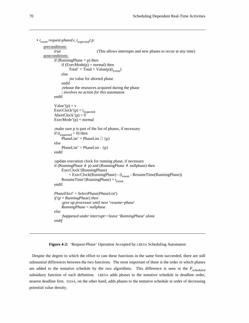
70 Scheduling Dependent Real-Time Activities
• t request-phase(v, t ) p:event expected
preconditions:true (This allows interrupts and new phases to occur at any time)
postconditions:if (RunningPhase = p) then
if (ExecMode(p) = normal) thenTotal’ = Total + Value(p)(t )event
else;no value for aborted phase
endif;release the resources acquired during the phase; involves no action for this automaton
endif
Value’(p) = vExecClock’(p) = texpectedAbortClock’(p) = 0ExecMode’(p) = normal
;make sure p is part of the list of phases, if necessaryif (t > 0) thenexpected
PhaseList’ = PhaseList ∪ {p}else
PhaseList’ = PhaseList - {p}endif
;update execution clock for running phase, if necessaryif (RunningPhase ≠ p) and (RunningPhase ≠ nullphase) then
ExecClock’(RunningPhase)= ExecClock(RunningPhase) - (t - ResumeTime(RunningPhase))event
ResumeTime’(RunningPhase) = teventendif
PhaseElect′ = SelectPhase(PhaseList′)if (p = RunningPhase) then
;give up processor until next ‘resume−phase′RunningPhase = nullphase
else;happened under interrupt−−leave ‘RunningPhase′ alone
endif
Figure 4-2: ‘Request-Phase’ Operation Accepted by LBESA Scheduling Automaton
Despite the degree to which the effort to cast these functions in the same form succeeded, there are still
substantial differences between the two functions. The most important of these is the order in which phases
are added to the tentative schedule by the two algorithms. This difference is seen in the Pscheduled
subsidiary function of each definition. LBESA adds phases to the tentative schedule in deadline order,
nearest deadline first. DASA, on the other hand, adds phases to the tentative schedule in order of decreasing
potential value density.
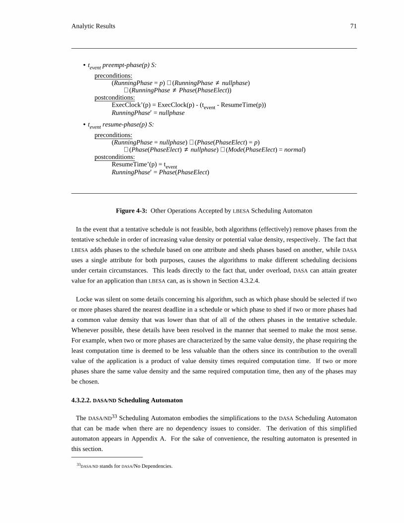
Analytic Results 71
• t preempt-phase(p) S:event
preconditions:(RunningPhase = p) ∧ (RunningPhase ≠ nullphase)
∧ (RunningPhase ≠ Phase(PhaseElect))postconditions:
ExecClock’(p) = ExecClock(p) - (t - ResumeTime(p))eventRunningPhase′ = nullphase
• t resume-phase(p) S:event
preconditions:(RunningPhase = nullphase) ∧ (Phase(PhaseElect) = p)
∧ (Phase(PhaseElect) ≠ nullphase) ∧ (Mode(PhaseElect) = normal)postconditions:
ResumeTime’(p) = teventRunningPhase′ = Phase(PhaseElect)
Figure 4-3: Other Operations Accepted by LBESA Scheduling Automaton
In the event that a tentative schedule is not feasible, both algorithms (effectively) remove phases from the
tentative schedule in order of increasing value density or potential value density, respectively. The fact that
LBESA adds phases to the schedule based on one attribute and sheds phases based on another, while DASA
uses a single attribute for both purposes, causes the algorithms to make different scheduling decisions
under certain circumstances. This leads directly to the fact that, under overload, DASA can attain greater
value for an application than LBESA can, as is shown in Section 4.3.2.4.
Locke was silent on some details concerning his algorithm, such as which phase should be selected if two
or more phases shared the nearest deadline in a schedule or which phase to shed if two or more phases had
a common value density that was lower than that of all of the others phases in the tentative schedule.
Whenever possible, these details have been resolved in the manner that seemed to make the most sense.
For example, when two or more phases are characterized by the same value density, the phase requiring the
least computation time is deemed to be less valuable than the others since its contribution to the overall
value of the application is a product of value density times required computation time. If two or more
phases share the same value density and the same required computation time, then any of the phases may
be chosen.
4.3.2.2. DASA/ND Scheduling Automaton
33The DASA/ND Scheduling Automaton embodies the simplifications to the DASA Scheduling Automaton
that can be made when there are no dependency issues to consider. The derivation of this simplified
automaton appears in Appendix A. For the sake of convenience, the resulting automaton is presented in
this section.
33DASA/ND stands for DASA/No Dependencies.
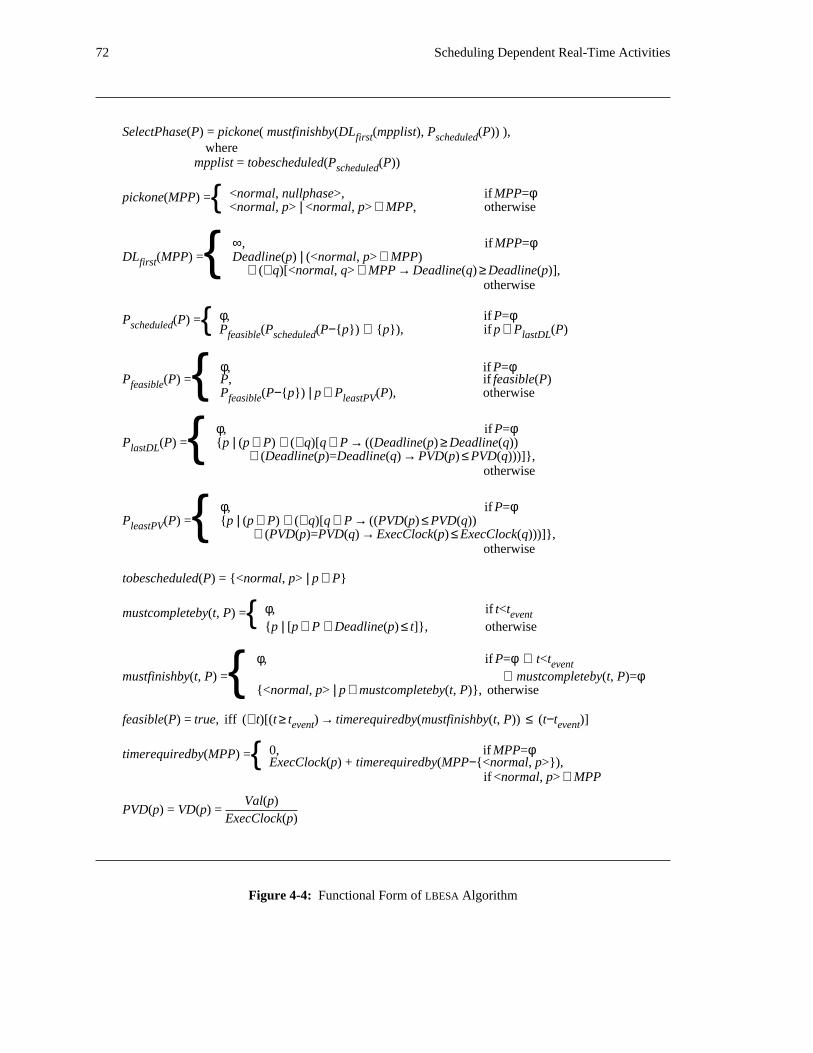
72 Scheduling Dependent Real-Time Activities
SelectPhase(P) = pickone( mustfinishby(DL (mpplist), P (P)) ),first scheduledwhere
mpplist = tobescheduled(P (P))scheduled
<normal, nullphase>, if MPP=φpickone(MPP) ={ <normal, p> | <normal, p> ∈ MPP, otherwise
∞, if MPP=φDL (MPP) = Deadline(p) | (<normal, p> ∈ MPP)first { ∧ (∀q)[<normal, q> ∈ MPP → Deadline(q) ≥ Deadline(p)],
otherwise
φ, if P=φP (P) =scheduled { P (P (P−{p}) ∪ {p}), if p ∈ P (P)feasible scheduled lastDL
φ, if P=φP (P) = P, if feasible(P)feasible { P (P−{p}) | p ∈ P (P), otherwisefeasible leastPV
φ, if P=φP (P) = {p | (p ∈ P) ∧ (∀q)[q ∈ P → ((Deadline(p) ≥ Deadline(q))lastDL { ∧ (Deadline(p)=Deadline(q) → PVD(p) ≤ PVD(q)))]},
otherwise
φ, if P=φP (P) = {p | (p ∈ P) ∧ (∀q)[q ∈ P → ((PVD(p) ≤ PVD(q))leastPV { ∧ (PVD(p)=PVD(q) → ExecClock(p) ≤ ExecClock(q)))]},
otherwise
tobescheduled(P) = {<normal, p> | p ∈ P}
φ, if t<tmustcompleteby(t, P) = event{{p | [p ∈ P ∧ Deadline(p) ≤ t]}, otherwise
φ, if P=φ ∨ t<teventmustfinishby(t, P) = ∨ mustcompleteby(t, P)=φ{ {<normal, p> | p ∈ mustcompleteby(t, P)}, otherwise
feasible(P) = true, iff (∀t)[(t ≥ t ) → timerequiredby(mustfinishby(t, P)) ≤ (t−t )]event event
0, if MPP=φtimerequiredby(MPP) ={ ExecClock(p) + timerequiredby(MPP−{<normal, p>}),if <normal, p> ∈ MPP
Val(p)PVD(p) = VD(p) =
ExecClock(p)
Figure 4-4: Functional Form of LBESA Algorithm
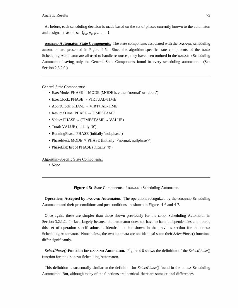
Analytic Results 73
As before, each scheduling decision is made based on the set of phases currently known to the automaton
and designated as the set {p , p , p , . . . }.0 1 2
DASA/ND Automaton State Components. The state components associated with the DASA/ND scheduling
automaton are presented in Figure 4-5. Since the algorithm-specific state components of the DASA
Scheduling Automaton are all used to handle resources, they have been omitted in the DASA/ND Scheduling
Automaton, leaving only the General State Components found in every scheduling automaton. (See
Section 2.3.2.9.)
General State Components:
• ExecMode: PHASE → MODE (MODE is either ‘normal’ or ‘abort’)
• ExecClock: PHASE → VIRTUAL-TIME
• AbortClock: PHASE → VIRTUAL-TIME
• ResumeTime: PHASE → TIMESTAMP
• Value: PHASE → (TIMESTAMP → VALUE)
• Total: VALUE (initially ‘0’)
• RunningPhase: PHASE (initially ‘nullphase’)
• PhaseElect: MODE × PHASE (initially ‘<normal, nullphase>’)
• PhaseList: list of PHASE (initially ‘φ’)
Algorithm-Specific State Components:
• None
Figure 4-5: State Components of DASA/ND Scheduling Automaton
Operations Accepted by DASA/ND Automaton. The operations recognized by the DASA/ND Scheduling
Automaton and their preconditions and postconditions are shown in Figures 4-6 and 4-7.
Once again, these are simpler than those shown previously for the DASA Scheduling Automaton in
Section 3.2.1.2. In fact, largely because the automaton does not have to handle dependencies and aborts,
this set of operation specifications is identical to that shown in the previous section for the LBESA
Scheduling Automaton. Nonetheless, the two automata are not identical since their SelectPhase() functions
differ significantly.
SelectPhase() Function for DASA/ND Automaton. Figure 4-8 shows the definition of the SelectPhase()
function for the DASA/ND Scheduling Automaton.
This definition is structurally similar to the definition for SelectPhase() found in the LBESA Scheduling
Automaton. But, although many of the functions are identical, there are some critical differences.
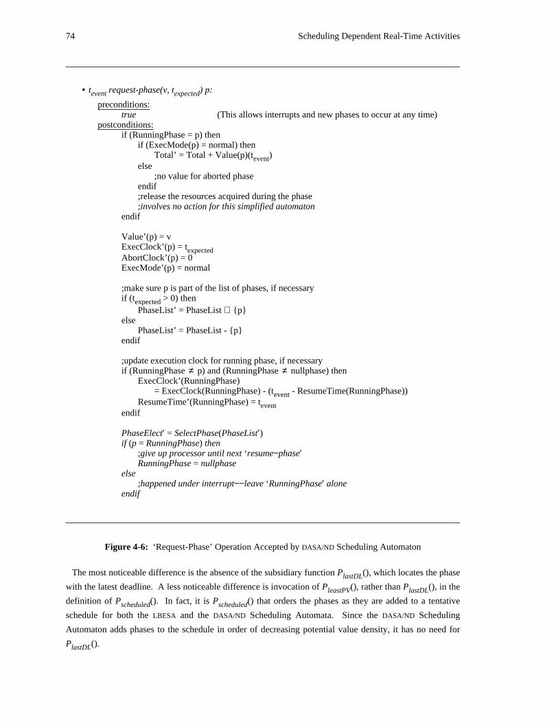
74 Scheduling Dependent Real-Time Activities
• t request-phase(v, t ) p:event expected
preconditions:true (This allows interrupts and new phases to occur at any time)
postconditions:if (RunningPhase = p) then
if (ExecMode(p) = normal) thenTotal’ = Total + Value(p)(t )event
else;no value for aborted phase
endif;release the resources acquired during the phase;involves no action for this simplified automaton
endif
Value’(p) = vExecClock’(p) = texpectedAbortClock’(p) = 0ExecMode’(p) = normal
;make sure p is part of the list of phases, if necessaryif (t > 0) thenexpected
PhaseList’ = PhaseList ∪ {p}else
PhaseList’ = PhaseList - {p}endif
;update execution clock for running phase, if necessaryif (RunningPhase ≠ p) and (RunningPhase ≠ nullphase) then
ExecClock’(RunningPhase)= ExecClock(RunningPhase) - (t - ResumeTime(RunningPhase))event
ResumeTime’(RunningPhase) = teventendif
PhaseElect′ = SelectPhase(PhaseList′)if (p = RunningPhase) then
;give up processor until next ‘resume−phase′RunningPhase = nullphase
else;happened under interrupt−−leave ‘RunningPhase′ alone
endif
Figure 4-6: ‘Request-Phase’ Operation Accepted by DASA/ND Scheduling Automaton
The most noticeable difference is the absence of the subsidiary function P (), which locates the phaselastDL
with the latest deadline. A less noticeable difference is invocation of P (), rather than P (), in theleastPV lastDL
definition of P (). In fact, it is P () that orders the phases as they are added to a tentativescheduled scheduled
schedule for both the LBESA and the DASA/ND Scheduling Automata. Since the DASA/ND Scheduling
Automaton adds phases to the schedule in order of decreasing potential value density, it has no need for
P ().lastDL
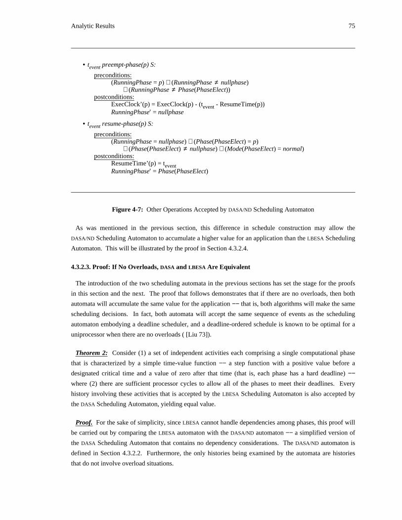
Analytic Results 75
• t preempt-phase(p) S:event
preconditions:(RunningPhase = p) ∧ (RunningPhase ≠ nullphase)
∧ (RunningPhase ≠ Phase(PhaseElect))postconditions:
ExecClock’(p) = ExecClock(p) - (t - ResumeTime(p))eventRunningPhase′ = nullphase
• t resume-phase(p) S:event
preconditions:(RunningPhase = nullphase) ∧ (Phase(PhaseElect) = p)
∧ (Phase(PhaseElect) ≠ nullphase) ∧ (Mode(PhaseElect) = normal)postconditions:
ResumeTime’(p) = teventRunningPhase′ = Phase(PhaseElect)
Figure 4-7: Other Operations Accepted by DASA/ND Scheduling Automaton
As was mentioned in the previous section, this difference in schedule construction may allow the
DASA/ND Scheduling Automaton to accumulate a higher value for an application than the LBESA Scheduling
Automaton. This will be illustrated by the proof in Section 4.3.2.4.
4.3.2.3. Proof: If No Overloads, DASA and LBESA Are Equivalent
The introduction of the two scheduling automata in the previous sections has set the stage for the proofs
in this section and the next. The proof that follows demonstrates that if there are no overloads, then both
automata will accumulate the same value for the application −− that is, both algorithms will make the same
scheduling decisions. In fact, both automata will accept the same sequence of events as the scheduling
automaton embodying a deadline scheduler, and a deadline-ordered schedule is known to be optimal for a
uniprocessor when there are no overloads ( [Liu 73]).
Theorem 2: Consider (1) a set of independent activities each comprising a single computational phase
that is characterized by a simple time-value function −− a step function with a positive value before a
designated critical time and a value of zero after that time (that is, each phase has a hard deadline) −−where (2) there are sufficient processor cycles to allow all of the phases to meet their deadlines. Every
history involving these activities that is accepted by the LBESA Scheduling Automaton is also accepted by
the DASA Scheduling Automaton, yielding equal value.
Proof. For the sake of simplicity, since LBESA cannot handle dependencies among phases, this proof will
be carried out by comparing the LBESA automaton with the DASA/ND automaton −− a simplified version of
the DASA Scheduling Automaton that contains no dependency considerations. The DASA/ND automaton is
defined in Section 4.3.2.2. Furthermore, the only histories being examined by the automata are histories
that do not involve overload situations.
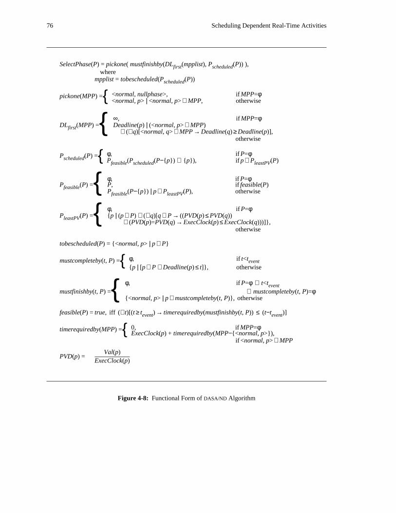
76 Scheduling Dependent Real-Time Activities
SelectPhase(P) = pickone( mustfinishby(DL (mpplist), P (P)) ),first scheduledwhere
mpplist = tobescheduled(P (P))scheduled
<normal, nullphase>, if MPP=φpickone(MPP) ={ <normal, p> | <normal, p> ∈ MPP, otherwise
∞, if MPP=φDL (MPP) = Deadline(p) | (<normal, p> ∈ MPP)first { ∧ (∀q)[<normal, q> ∈ MPP → Deadline(q) ≥ Deadline(p)],
otherwise
φ, if P=φP (P) =scheduled { P (P (P−{p}) ∪ {p}), if p ∈ P (P)feasible scheduled leastPV
φ, if P=φP (P) = P, if feasible(P)feasible { P (P−{p}) | p ∈ P (P), otherwisefeasible leastPV
φ, if P=φP (P) = {p | (p ∈ P) ∧ (∀q)[q ∈ P → ((PVD(p) ≤ PVD(q))leastPV { ∧ (PVD(p)=PVD(q) → ExecClock(p) ≤ ExecClock(q)))]},
otherwise
tobescheduled(P) = {<normal, p> | p ∈ P}
φ, if t<tmustcompleteby(t, P) = event{{p | [p ∈ P ∧ Deadline(p) ≤ t]}, otherwise
φ, if P=φ ∨ t<teventmustfinishby(t, P) = ∨ mustcompleteby(t, P)=φ{ {<normal, p> | p ∈ mustcompleteby(t, P)}, otherwise
feasible(P) = true, iff (∀t)[(t ≥ t ) → timerequiredby(mustfinishby(t, P)) ≤ (t−t )]event event
0, if MPP=φtimerequiredby(MPP) ={ ExecClock(p) + timerequiredby(MPP−{<normal, p>}),if <normal, p> ∈ MPP
Val(p)PVD(p) =
ExecClock(p)
Figure 4-8: Functional Form of DASA/ND Algorithm
Analytic Results 77
The proof is performed by induction over the events in an accepted history.
Basis. Show that (1) if LBESA accepts the first event in a history, DASA/ND will also accept it, (2)
RunningPhase, PhaseList, PhaseElect, and Total are the same for both automata, and (3) Value, ExecClock,
ExecMode, and ResumeTime are the same for each active phase in both automata.
Initially,
RunningPhase = nullphasePhaseList = φPhaseElect = <normal, nullphase>Total = 0
As a result, the only event whose precondition for LBESA may be satisfied is ‘request-phase.’ Therefore,
the first event in any history that LBESA will accept must be a ‘request-phase.’
Let this first event be denoted:
t request−phase(v, t ) pevent1 expected1 1
LBESA accepts this event −− its precondition for accepting it is true −− and as dictated by its
postconditions, it sets:
Total′ = 0Value′(p ) = v1ExecClock′(p ) = t1 expected1ExecMode′(p ) = normal1PhaseList′ = {p }1PhaseElect′ = SelectPhase(PhaseList)
<normal, p >, if feasible({p })= 1 1{ <normal, nullphase>, otherwise
DASA/ND also accepts this event −− its precondition is also true −− and, the state component changes
induced by the postconditions for the event include those made by LBESA.
Therefore, DASA/ND accepts the first event in any history accepted by LBESA. Furthermore,
RunningPhase, PhaseList, PhaseElect, and Total are identical in both automata after accepting this event.
And finally, Value, ExecClock, and ExecMode are the same in both automata after accepting the event for
the only currently active phase, p , while ResumeTime is not yet defined for any phase in either automata1
−− and so is trivially the same in both.
Inductive Step. Given that DASA/ND has accepted the first n events in a history that LBESA accepts; that
RunningPhase, PhaseList, PhaseElect, and Total are the same for both automata after accepting those
events; and that Value, ExecClock, ExecMode, and ResumeTime are the same in both automata for eachstactive phase after accepting those events; show that DASA/ND will also accept the n+1 event in the history
if LBESA accepts it, that RunningPhase, PhaseList, PhaseElect, and Total will be the same in each
automaton after that event is accepted, and that Value, ExecClock, ExecMode, and ResumeTime will be thestsame in each automaton for each active phase after the n+1 event is accepted.
78 Scheduling Dependent Real-Time Activities
LBESA may accept any event for which the precondition is satisfied. In this case, it may accept an
appropriate:
• ‘preempt-phase’
• ‘resume-phase’
• ‘request-phase’
The precondition for accepting each of these events is the same in both automata. The preconditions
depend only on the values of RunningPhase, PhaseElect, and the parameter p. Hence if LBESA accepts thestn+1 event, DASA/ND will also accept it since, by inductive hypothesis, it has the same values for the
relevant state components, the same parameter values, and the same precondition as LBESA.
Next, it should be demonstrated that RunningPhase, PhaseList, PhaseElect, and Total are the same forstboth automata after the n+1 event is accepted, and that Value, ExecClock, ExecMode, and ResumeTime
are the same for both automata for each active phase after that event is accepted.
Consider each of the three possible events:1. ‘preempt-phase’ −− in both automata, RunningPhase′ is set to nullphase while PhaseElect
remains unchanged, and therefore equal. Also in both automata, ExecClock′(p) is assigned anew value. The formula used to update ExecClock′(p) is the same in both automata,ExecClock(p) and ResumeTime(p) are the same in both automata by inductive assumption,
stand t is the same in both since it is part of the n+1 event and so is independent of theeventstate of the automata. Therefore, ExecClock′(p) will be the same in both automata.
2. ‘resume-phase’ −− in both automata, RunningPhase is set to PhaseElect, which has the samevalue in both automata after accepting the first n events, while PhaseElect remainsunchanged, and therefore equal, in both automata. Also, ResumeTime′(p) is set to t . Thiseventassignment results in the same state for ResumeTime′(p) in both automata since ResumeTimewas the same in both automata for all active phases after the first n events had been accepted
stand t is the same for both automata because it is part of the n+1 event and so iseventindependent of the states of the automata.
3. ‘request-phase’ −−• RunningPhase: in both automata, RunningPhase′ may conditionally be set to nullphase;
in each automaton, the condition under which this is done −− p = RunningPhase −− isthe same, RunningPhase is the same by inductive hypothesis, and p is the same since it
stis part of the n+1 event and has a value that is independent of the state of theautomaton.
• PhaseList: in both automata, PhaseList′ will conditionally be set to eitherPhaseList ∪ {p} or PhaseList − {p}; in each automaton, the condition under which thisis done −− t > 0 −− is the same, PhaseList is the same by inductive hypothesis,expected
stand p and t are the same since they are part of the n+1 event and have valuesexpectedthat are independent of the state of the automaton.
• PhaseElect: in both automata, PhaseElect′ is set to SelectPhase(PhaseList′). As arguedin the previous bullet, PhaseList′ is the same in both automata. Now consider thefunction SelectPhase() for each automaton. Most of the subordinate functions involvedin the definition of SelectPhase() are identical in both automata. In fact the onlysubordinate function that differs is P () −− although the form is the same inscheduledboth, the specific ordering of recursive functional evaluations is different in the twoautomaton definitions.
It is given that there are sufficient processor cycles available to allow all of the phases
Analytic Results 79
to meet all of their deadlines. In terms of the mathematical formulation of theseautomata, this is equivalent to saying that (∀P)feasible(P) = true −− that is, it is
34feasible to schedule all of the known phases at any given time. In that case, for bothautomata the definition of P () can be simplified fromfeasible
φ, if P=φP (P) = P, if feasible(P)feasible { P (P−{p}) | p ∈ P (P), otherwisefeasible leastPV
to
φ, if P=φP (P) =feasible { P, if feasible(P)
and, finally, to
P (P) = Pfeasible
Since P () acts as an identity function, the definition of P () can also befeasible scheduledsimplified from:
φ, if P=φP (P) =scheduled { P (P (P−{p}) ∪ {p}), if p ∈ P (P)feasible scheduled x
where P () is P () for LBESA and P () for DASA/ND, to:x lastDL leastPV
φ, if P=φP (P) =scheduled { P (P−{p}) ∪ {p}, if p ∈ P (P)scheduled x
which is equivalent to:
P (P) = Pscheduled
Of course, the definitions of SelectPhase() for both automata are now exactly the same.The evaluation of SelectPhase(PhaseList′) depends on the values of PhaseList′,ExecClock′, and Value′, all of which are shown to be the same for both automata after
stthe n+1 event in the history is accepted. The value also depends on t which is theeventstsame for both automata since it is part of the n+1 event and is therefore independent
of the state of the automata. Consequently, PhaseElect′ will be the same for bothautomata.
• Total: in both automata, if RunningPhase = p and ExecMode(p) = normal, Total′ willbe set equal to Total + Value(p)(t ); otherwise, Total′ will remain unchanged by theevent
stn+1 event. Since by inductive hypothesis RunningPhase and ExecMode are the samestin both automata, and since p is the same in both automata since it is part of the n+1
event and consequently has a value that is independent of the state of the automata, thestcondition under which Total′ will be updated by the n+1 event is the same in both
automata. Also, since Total and Value are the same in both automata by inductivesthypothesis, and p and t are both part of the n+1 event, the computed valueevent
assigned to Total′ is identical in both automata.
• Value: in both automata, Value′(p) is unconditionally set to v; in each automaton, p andstv are the same since they are part of the n+1 event and have values that are
independent of the state of the automaton. Since Value had been the same in bothautomata after n events were accepted and since both automata set Value′(p) = v, Value′is the same in both.
• ExecClock: in both automata, ExecClock′(p) is unconditionally set to t ; in eachexpected
34This property is maintained through an entire history because both automata accept deadline-ordered histories if there are nooverload conditions, and a deadline-ordered schedule will be guaranteed to meet all of the deadlines if there are sufficient processingcycles available.
80 Scheduling Dependent Real-Time Activities
stautomaton, p and t are the same since they are part of the n+1 event and haveexpectedvalues that are independent of the state of the automaton. Therefore, ExecClock′(p) isthe same in both automata.
In addition, both automata conditionally set ExecClock′(RunningPhase); theconditional test used by both automata is the same, as are the values of RunningPhase
st(by inductive hypothesis) and p (as part of the n+1 event) used when performing thetest. Therefore, either both or neither of the automata will perform the assignment toExecClock(RunningPhase). Furthermore, the value assigned is the same for bothautomata since ExecClock(RunningPhase) and ResumeTime(RunningPhase) are thesame in both automata according to the inductive assumption, t is the same since itevent
stis part of the n+1 event, and the expression used to determine the new value forExecClock(RunningPhase) is the same for both automata and depends on only thesevalues.
Since ExecClock had been the same in both automata after n events were accepted andsince both automata set ExecClock′(p) and ExecClock′(RunningPhase) identically,ExecClock′ is the same in both.
• ExecMode: in both automata, ExecMode′(p) is unconditionally set to normal; in eachstautomaton, p is the same since it is part of the n+1 event and has a value that is
independent of the state of the automaton. Since ExecMode had been the same in bothautomata after n events were accepted and since both automata setExecMode′(p) = normal, ExecMode′ is the same in both.
• ResumeTime: in both automata, ResumeTime′(RunningPhase) is conditionally set tot . The condition under which this is done is the same for both automata andeventdepends only on the values of RunningPhase and p which are the same for each
stautomata by inductive hypothesis and as part of the n+1 event, respectively.Therefore, either both or neither automaton sets the value. Since t is the same foreventboth automata, they will both assign the same value to ResumeTime′(RunningPhase) ifthey perform the assignment. Since ResumeTime had been the same in both automataafter n events were accepted and since both automata set ResumeTime′(RunningPhase)
stidentically for the n+1 event, ResumeTime′ is the same in both.
stThus, if LBESA accepts any of these event types as the n+1 event in a history, so will DASA/ND, and the
significant state components of each automaton will be the same at that point.
Therefore, by induction, DASA/ND, and hence DASA itself, accepts any history accepted by LBESA under
the conditions outlined in the theorem statement. Furthermore, because the state component Total will be
the same in both automata after accepting a history, both will yield the same value for any history that they
accept.
EndOfProof
4.3.2.4. Proof: With Overloads, DASA May Exceed LBESA
The preceding section showed that the DASA Scheduling Automaton performed well when there were no
overloads. In this section, it is shown that, when there are overloads, the DASA Scheduling Automaton may
accept histories that yield higher values for the application than any history that may be accepted by the
LBESA Scheduling Automaton. The reason for this has been mentioned previously in Sections 4.3.2.1 and
4.3.2.2: although both algorithms use similar value density metrics, they construct schedules in different
ways, potentially resulting in situations where LBESA sheds some phases unnecessarily.
Analytic Results 81
Once again, for the sake of simplicity, since no dependencies are involved, the DASA/ND Scheduling
Automaton, rather than the DASA Scheduling Automaton, is use in the following proof. The result,
however, applies to the DASA Scheduling Automaton as well.
Theorem 3: Consider (1) a set of independent activities each comprising a single computational phase
that is characterized by a simple time-value function −− a step function with a positive value before a
designated critical time and a value of zero after that time (that is, each phase has a hard deadline) −−where (2) there are insufficient processor cycles to allow all of the phases to meet their deadlines. The
DASA/ND Scheduling Automaton may accept a history with a greater value than any history the LBESA
Scheduling Automaton can accept involving the same phases and the same scheduling parameters (time-
value functions and required computation times).
Proof. This proof is carried out by constructing an example.
Intuitively, LBESA constructs a complete schedule by considering each phase in order of its deadline,
nearest deadline first. As each phase is considered, an estimate is performed to determine whether there is
an overload situation. In that case, it discards the phases with the lowest value densities until a feasible
schedule is obtained. In the process, it may discard some phases unnecessarily. DASA/ND also constructs a
schedule from scratch; however, it begins with the phase having the greatest value density and considers
subsequent phases in decreasing order of value density. Each phase is included in the schedule in order of
its deadline if the schedule −− including that phase −− is feasible. Since this approach includes as many
high value density phases as possible and only discards those phases that cannot be added to the schedule,
rather than those that have lower value densities than one that must be discarded, it avoids the problem that
LBESA encounters.
An example of DASA/ND accepting a history with a greater value than LBESA will accept can be
constructed using phases with the following parameters:
Phase Deadline Required ValueComputation Time
p1 2t t + 1 v1a a
p2 2t t v2a a
p3 2t - 1 t - 1 v3a a
Let t > 1 and v1, v2, v3 > 0. Also, let v1/(t +1)>v2/t >v3/(t −1) indicate the initial relationship of thea a a a
value densities of the three phases, p1, p2, and p3, respectively. Now consider the following history, H :1
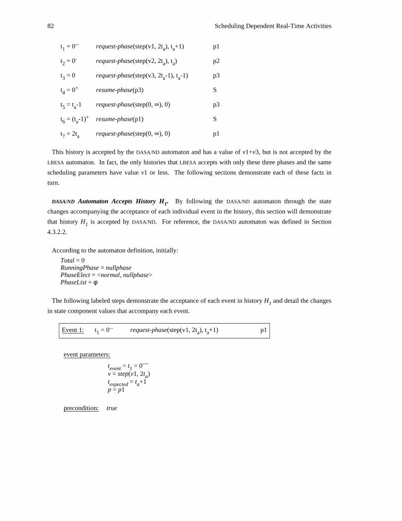
82 Scheduling Dependent Real-Time Activities
--t = 0 request-phase(step(v1, 2t ), t +1) p11 a a
-t = 0 request-phase(step(v2, 2t ), t ) p22 a a
t = 0 request-phase(step(v3, 2t -1), t -1) p33 a a
+t = 0 resume-phase(p3) S4
t = t -1 request-phase(step(0, ∞), 0) p35 a
+t = (t -1) resume-phase(p1) S6 a
t = 2t request-phase(step(0, ∞), 0) p17 a
This history is accepted by the DASA/ND automaton and has a value of v1+v3, but is not accepted by the
LBESA automaton. In fact, the only histories that LBESA accepts with only these three phases and the same
scheduling parameters have value v1 or less. The following sections demonstrate each of these facts in
turn.
DASA/ND Automaton Accepts History H . By following the DASA/ND automaton through the state1
changes accompanying the acceptance of each individual event in the history, this section will demonstrate
that history H is accepted by DASA/ND. For reference, the DASA/ND automaton was defined in Section1
4.3.2.2.
According to the automaton definition, initially:
Total = 0RunningPhase = nullphasePhaseElect = <normal, nullphase>PhaseList = φ
The following labeled steps demonstrate the acceptance of each event in history H and detail the changes1
in state component values that accompany each event.
--Event 1: t = 0 request-phase(step(v1, 2t ), t +1) p11 a a
event parameters:−−t = t = 0event 1
v = step(v1, 2t )at = t +1expected ap = p1
precondition: true
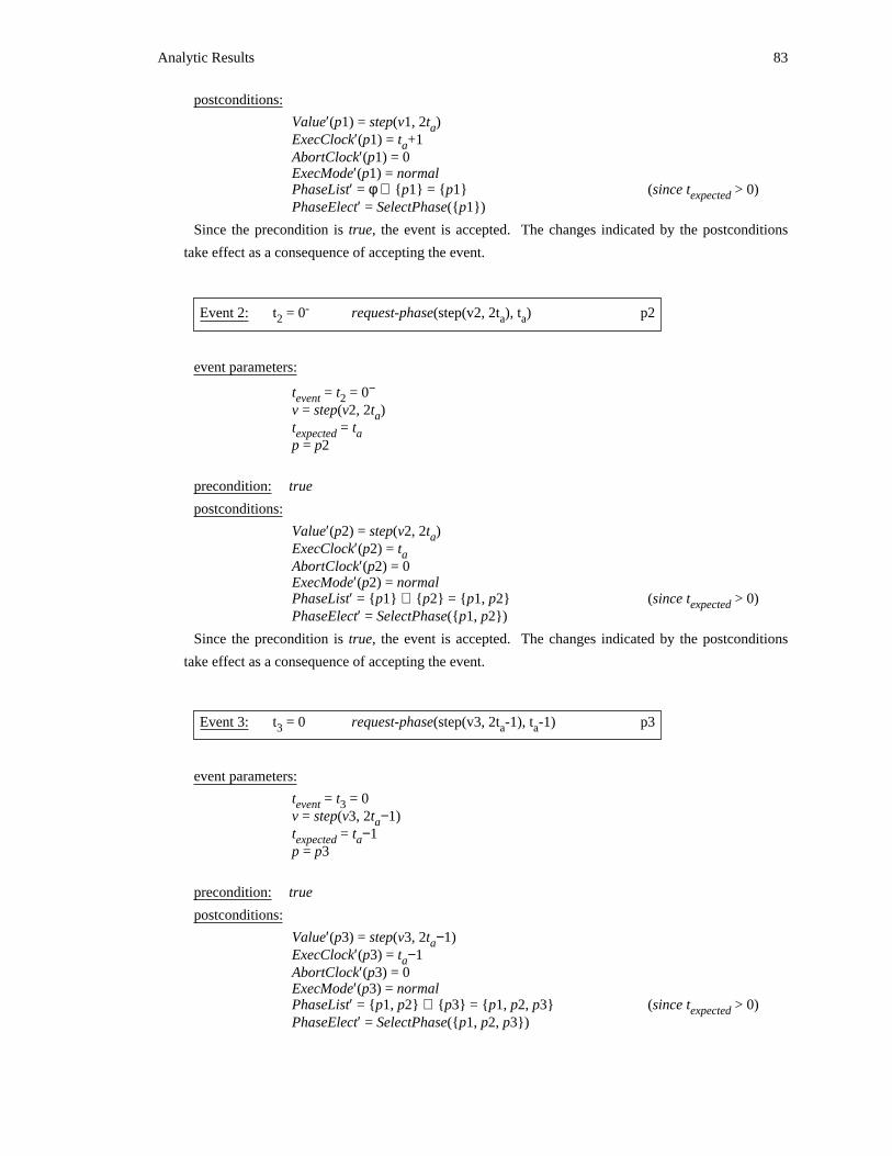
Analytic Results 83
postconditions:
Value′(p1) = step(v1, 2t )aExecClock′(p1) = t +1aAbortClock′(p1) = 0ExecMode′(p1) = normalPhaseList′ = φ ∪ {p1} = {p1} (since t > 0)expectedPhaseElect′ = SelectPhase({p1})
Since the precondition is true, the event is accepted. The changes indicated by the postconditions
take effect as a consequence of accepting the event.
-Event 2: t = 0 request-phase(step(v2, 2t ), t ) p22 a a
event parameters:−t = t = 0event 2
v = step(v2, 2t )at = texpected ap = p2
precondition: true
postconditions:
Value′(p2) = step(v2, 2t )aExecClock′(p2) = taAbortClock′(p2) = 0ExecMode′(p2) = normalPhaseList′ = {p1} ∪ {p2} = {p1, p2} (since t > 0)expectedPhaseElect′ = SelectPhase({p1, p2})
Since the precondition is true, the event is accepted. The changes indicated by the postconditions
take effect as a consequence of accepting the event.
Event 3: t = 0 request-phase(step(v3, 2t -1), t -1) p33 a a
event parameters:
t = t = 0event 3v = step(v3, 2t −1)at = t −1expected ap = p3
precondition: true
postconditions:
Value′(p3) = step(v3, 2t −1)aExecClock′(p3) = t −1aAbortClock′(p3) = 0ExecMode′(p3) = normalPhaseList′ = {p1, p2} ∪ {p3} = {p1, p2, p3} (since t > 0)expectedPhaseElect′ = SelectPhase({p1, p2, p3})
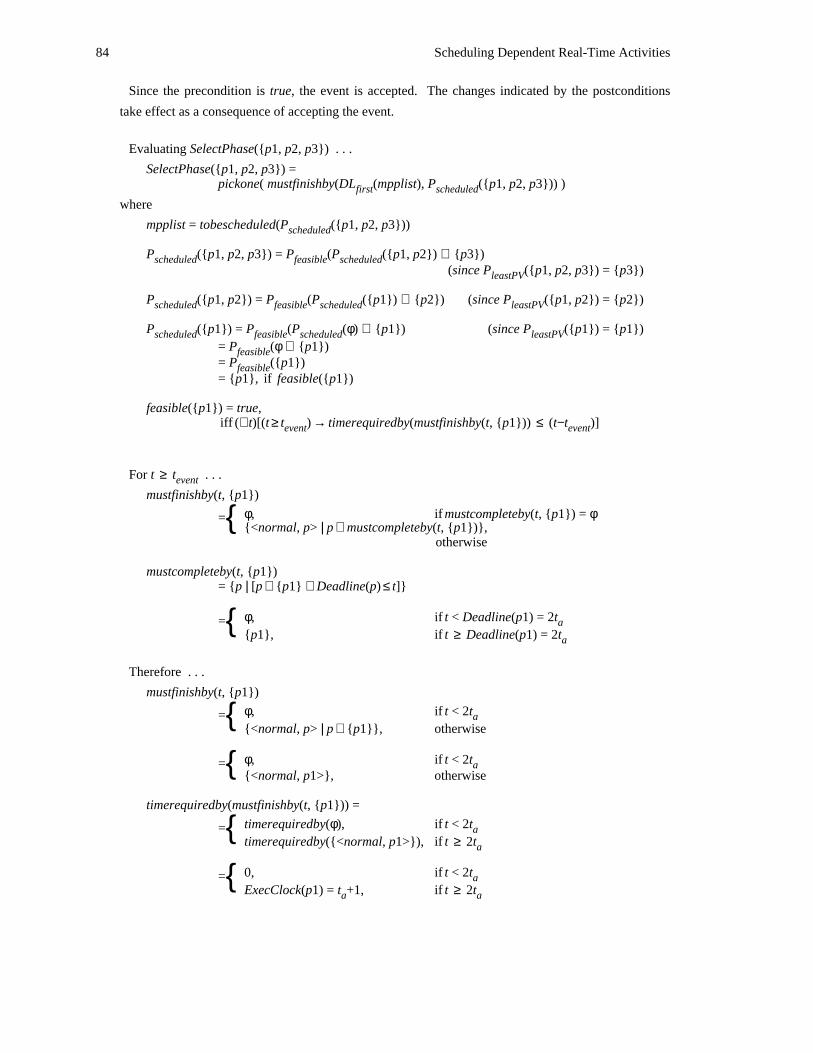
84 Scheduling Dependent Real-Time Activities
Since the precondition is true, the event is accepted. The changes indicated by the postconditions
take effect as a consequence of accepting the event.
Evaluating SelectPhase({p1, p2, p3}) . . .
SelectPhase({p1, p2, p3}) =pickone( mustfinishby(DL (mpplist), P ({p1, p2, p3})) )first scheduled
where
mpplist = tobescheduled(P ({p1, p2, p3}))scheduled
P ({p1, p2, p3}) = P (P ({p1, p2}) ∪ {p3})scheduled feasible scheduled(since P ({p1, p2, p3}) = {p3})leastPV
P ({p1, p2}) = P (P ({p1}) ∪ {p2}) (since P ({p1, p2}) = {p2})scheduled feasible scheduled leastPV
P ({p1}) = P (P (φ) ∪ {p1}) (since P ({p1}) = {p1})scheduled feasible scheduled leastPV= P (φ ∪ {p1})feasible= P ({p1})feasible= {p1}, if feasible({p1})
feasible({p1}) = true,iff (∀t)[(t ≥ t ) → timerequiredby(mustfinishby(t, {p1})) ≤ (t−t )]event event
For t ≥ t . . .event
mustfinishby(t, {p1})
φ, if mustcompleteby(t, {p1}) = φ={ {<normal, p> | p ∈ mustcompleteby(t, {p1})},otherwise
mustcompleteby(t, {p1})= {p | [p ∈ {p1} ∧ Deadline(p) ≤ t]}
φ, if t < Deadline(p1) = 2t= a{{p1}, if t ≥ Deadline(p1) = 2ta
Therefore . . .
mustfinishby(t, {p1})
φ, if t < 2t= a{{<normal, p> | p ∈ {p1}}, otherwise
φ, if t < 2t= a{ {<normal, p1>}, otherwise
timerequiredby(mustfinishby(t, {p1})) =
timerequiredby(φ), if t < 2t= a{timerequiredby({<normal, p1>}), if t ≥ 2ta
0, if t < 2t= a{ExecClock(p1) = t +1, if t ≥ 2ta a
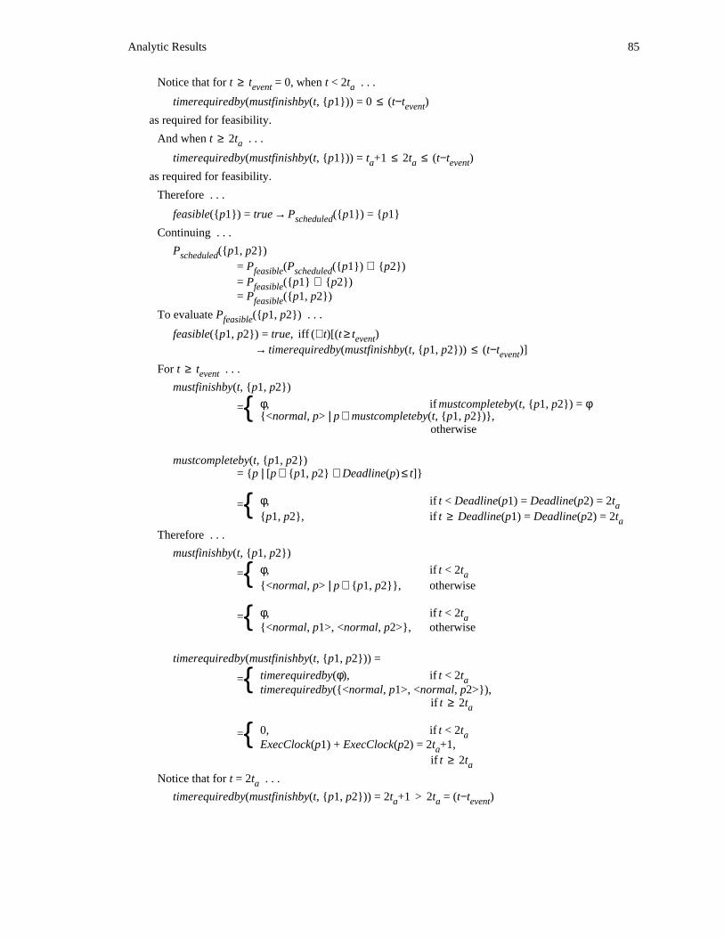
Analytic Results 85
Notice that for t ≥ t = 0, when t < 2t . . .event a
timerequiredby(mustfinishby(t, {p1})) = 0 ≤ (t−t )event
as required for feasibility.
And when t ≥ 2t . . .a
timerequiredby(mustfinishby(t, {p1})) = t +1 ≤ 2t ≤ (t−t )a a event
as required for feasibility.
Therefore . . .
feasible({p1}) = true → P ({p1}) = {p1}scheduled
Continuing . . .
P ({p1, p2})scheduled= P (P ({p1}) ∪ {p2})feasible scheduled= P ({p1} ∪ {p2})feasible= P ({p1, p2})feasible
To evaluate P ({p1, p2}) . . .feasible
feasible({p1, p2}) = true, iff (∀t)[(t ≥ t )event→ timerequiredby(mustfinishby(t, {p1, p2})) ≤ (t−t )]event
For t ≥ t . . .event
mustfinishby(t, {p1, p2})
φ, if mustcompleteby(t, {p1, p2}) = φ={ {<normal, p> | p ∈ mustcompleteby(t, {p1, p2})},otherwise
mustcompleteby(t, {p1, p2})= {p | [p ∈ {p1, p2} ∧ Deadline(p) ≤ t]}
φ, if t < Deadline(p1) = Deadline(p2) = 2t= a{{p1, p2}, if t ≥ Deadline(p1) = Deadline(p2) = 2ta
Therefore . . .
mustfinishby(t, {p1, p2})
φ, if t < 2t= a{{<normal, p> | p ∈ {p1, p2}}, otherwise
φ, if t < 2t= a{ {<normal, p1>, <normal, p2>}, otherwise
timerequiredby(mustfinishby(t, {p1, p2})) =
timerequiredby(φ), if t < 2t= a{ timerequiredby({<normal, p1>, <normal, p2>}),if t ≥ 2ta
0, if t < 2t= a{ ExecClock(p1) + ExecClock(p2) = 2t +1,aif t ≥ 2ta
Notice that for t = 2t . . .a
timerequiredby(mustfinishby(t, {p1, p2})) = 2t +1 > 2t = (t−t )a a event
86 Scheduling Dependent Real-Time Activities
This violates the requirement for feasibility. Therefore . . .
feasible({p1, p2}) = false→ P ({p1, p2}) = P ({p1}) (since P ({p1, p2}) = {p2})feasible feasible leastPV
= {p1} (as shown above)→ P ({p1, p2}) = {p1} (since P ({p1, p2}) = P ({p1, p2}))scheduled scheduled feasible
Continuing . . .
P ({p1, p2, p3})scheduled= P (P ({p1, p2}) ∪ {p3}) (as shown above)feasible scheduled= P ({p1} ∪ {p3})feasible= P ({p1, p3})feasible
To evaluate P ({p1, p3}) . . .feasible
feasible({p1, p3}) = true, iff (∀t)[(t ≥ t )event→ timerequiredby(mustfinishby(t, {p1, p3})) ≤ (t−t )]event
For t ≥ t . . .event
mustfinishby(t, {p1, p3})
φ, if mustcompleteby(t, {p1, p3}) = φ={ {<normal, p> | p ∈ mustcompleteby(t, {p1, p3})},otherwise
mustcompleteby(t, {p1, p3})= {p | [p ∈ {p1, p3} ∧ Deadline(p) ≤ t]}
φ, if t < Deadline(p3) = 2t −1a{p3}, if Deadline(p3) = 2t −1 ≤ ta= < Deadline(p1) = 2t{ a{p1, p3}, if t ≥ Deadline(p1) = 2ta
Therefore . . .
mustfinishby(t, {p1, p3})
φ, if t < 2t −1a= {<normal, p> | p ∈ {p3}}, if 2t −1 ≤ t < 2ta a{
{<normal, p> | p ∈ {p1, p3}}, if 2t ≤ ta
φ, if t < 2t −1a= {<normal, p3>}, if 2t −1 ≤ t < 2ta a{
{<normal, p1>, <normal, p3>}, if 2t ≤ ta
timerequiredby(mustfinishby(t, {p1, p3}))
timerequiredby(φ), if t < 2t −1a= timerequiredby({<normal, p3>}), if 2t −1 ≤ t < 2ta a{
timerequiredby({<normal, p1>, <normal, p3>}),if 2t ≤ ta
0, if t < 2t −1a= ExecClock(p3) = t −1, if 2t −1 ≤ t < 2ta a a{
ExecClock(p1) + ExecClock(p3) = 2t ,aif 2t ≤ ta
Analytic Results 87
Notice that for t ≥ t = 0, when t < 2t −1 . . .event a
timerequiredby(mustfinishby(t, {p1, p3})) = 0 ≤ (t−t )event
as required for feasibility.
When 2t −1 ≤ t < 2t . . .a a
timerequiredby(mustfinishby(t, {p1, p3})) = t −1 < 2t −1 ≤ (t−t )a a event
as required for feasibility.
And when t ≥ 2t . . .a
timerequiredby(mustfinishby(t, {p1, p3})) = 2t ≤ (t−t )a event
as required for feasibility.
Therefore . . .
feasible({p1, p3}) = true→ P ({p1, p3}) = {p1, p3}feasible→ P ({p1, p2, p3}) = {p1, p3}scheduled
So P ({p1, p2, p3}), the set of phases that can feasibly be executed so that each will meet itsscheduled
deadline while contributing the maximum value to the system for the investment of a given amount of
time, has now been determined. Next, the individual phase from this set that will be executed first
must be determined.
mpplist = tobescheduled(P ({p1, p2, p3}))scheduled= tobescheduled({p1, p3})= {<normal, p1>, <normal, p3>}
DL (mpplist) = DL ({<normal, p1>, <normal, p3>})first first= 2t −1a
mustfinishby(DL (mpplist), P ({p1, p2, p3}))first scheduled= mustfinishby(2t −1, {p1, p3})a= {<normal, p> | p ∈ mustcompleteby(2t −1, {p1, p3})}a
(assuming mustcompleteby(2t −1, {p1, p3}) ≠ φ)a= {<normal, p> | p ∈ {p1, p3} ∧ Deadline(p) ≤ 2t −1}a= {<normal, p> | p ∈ {p3}} (note that mustcompleteby(2t −1, {p1, p3}) ≠ φ)a= {<normal, p3>}
Finally . . .
PhaseElect′ = SelectPhase({p1, p2, p3})= pickone( mustfinishby(DL (mpplist), P ({p1, p2, p3})) )first scheduled= pickone({<normal, p3>})= <normal, p3>
+Event 4: t = 0 resume-phase(p3) S4
event parameters:+t = t = 0event 4
p = p3
88 Scheduling Dependent Real-Time Activities
precondition:
(RunningPhase = nullphase) ∧ (Phase(PhaseElect) = p3)∧ (Phase(PhaseElect) ≠ nullphase) ∧ (Mode(PhaseElect) = normal)
≡
(RunningPhase = nullphase) ∧ (Phase(<normal, p3>) = p3)∧ (Phase(<normal, p3>) ≠ nullphase) ∧ (Mode(<normal, p3>) = normal)
≡
true
postconditions:+ResumeTime′(p3) = 0
RunningPhase′ = Phase(PhaseElect) = Phase(<normal, p3>) = p3
Since the precondition is shown to be true, the event is accepted and the postconditions cause the
indicated changes in the state components.
Event 5: t = t -1 request-phase(step(0, ∞), 0) p35 a
event parameters:
t = t = t −1event 5 av = step(0, ∞)t = 0expectedp = p3
precondition: true
postconditions:
Total′ = 0+Value(p3)(t −1) (since RunningPhase=p3 ∧ ExecMode(p3)=normal)a= step(v3, 2t −1)(t −1)a a= v3
Value′(p3) = step(0, ∞)ExecClock′(p3) = 0AbortClock′(p3) = 0ExecMode′(p3) = normalPhaseList′ = {p1, p2, p3} − {p3} = {p1, p2} (since t = 0)expectedPhaseElect′ = SelectPhase({p1, p2})RunningPhase′ = nullphase (since p3 = RunningPhase)
Since the precondition is true, the event is accepted. The changes indicated by the postconditions
take effect as a consequence of accepting the event.
Evaluating SelectPhase({p1, p2}) . . .
SelectPhase({p1, p2}) = pickone( mustfinishby(DL (mpplist), P ({p1, p2})) )first scheduled
where
mpplist = tobescheduled(P ({p1, p2}))scheduled
P ({p1, p2}) = P (P ({p1}) ∪ {p2}) (since P ({p1, p2}) = {p2})scheduled feasible scheduled leastPV
Analytic Results 89
P ({p1}) = P (P (φ) ∪ {p1}) (since P ({p1}) = {p1})scheduled feasible scheduled leastPV= P (φ ∪ {p1})feasible= P ({p1})feasible= {p1}, if feasible({p1})
feasible({p1}) = true,iff (∀t)[(t ≥ t ) → timerequiredby(mustfinishby(t, {p1})) ≤ (t−t )]event event
As before, for t ≥ t = t −1 . . .event a
mustfinishby(t, {p1})
φ, if mustcompleteby(t, {p1}) = φ={ {<normal, p> | p ∈ mustcompleteby(t, {p1})},otherwise
mustcompleteby(t, {p1})= {p | [p ∈ {p1} ∧ Deadline(p) ≤ t]}
φ, if t < Deadline(p1) = 2t= a{{p1}, if t ≥ Deadline(p1) = 2ta
Therefore . . .
mustfinishby(t, {p1})
φ, if t < 2t= a{{<normal, p> | p ∈ {p1}}, otherwise
φ, if t < 2t= a{ {<normal, p1>}, otherwise
timerequiredby(mustfinishby(t, {p1}))
timerequiredby(φ), if t < 2t= a{timerequiredby({<normal, p1>}), if t ≥ 2ta
0, if t < 2t= a{ExecClock(p1) = t +1, if t ≥ 2ta a
Notice that for t ≥ t = t −1, when t < 2t . . .event a a
timerequiredby(mustfinishby(t, {p1})) = 0 ≤ (t−t )event
as required for feasibility.
And when t ≥ 2t . . .a
timerequiredby(mustfinishby(t, {p1})) = t +1 ≤ (t−t )a event
as required for feasibility.
Therefore . . .
feasible({p1}) = true → P ({p1}) = {p1}scheduled
Continuing . . .
P ({p1, p2})scheduled= P (P ({p1}) ∪ {p2}) (as shown above)feasible scheduled= P ({p1} ∪ {p2})feasible= P ({p1, p2})feasible
feasible({p1, p2}) = true, iff (∀t)[(t ≥ t )event→ timerequiredby(mustfinishby(t, {p1, p2})) ≤ (t−t )]event
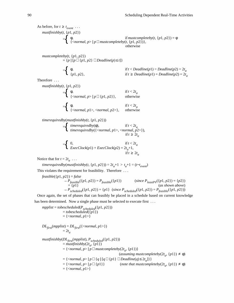
90 Scheduling Dependent Real-Time Activities
As before, for t ≥ t . . .event
mustfinishby(t, {p1, p2})
φ, if mustcompleteby(t, {p1, p2}) = φ={ {<normal, p> | p ∈ mustcompleteby(t, {p1, p2})},otherwise
mustcompleteby(t, {p1, p2})= {p | [p ∈ {p1, p2} ∧ Deadline(p) ≤ t]}
φ, if t < Deadline(p1) = Deadline(p2) = 2t= a{{p1, p2}, if t ≥ Deadline(p1) = Deadline(p2) = 2ta
Therefore . . .
mustfinishby(t, {p1, p2})
φ, if t < 2t= a{{<normal, p> | p ∈ {p1, p2}}, otherwise
φ, if t < 2t= a{ {<normal, p1>, <normal, p2>}, otherwise
timerequiredby(mustfinishby(t, {p1, p2}))
timerequiredby(φ), if t < 2t= a{ timerequiredby({<normal, p1>, <normal, p2>}),if t ≥ 2ta
0, if t < 2t= a{ ExecClock(p1) + ExecClock(p2) = 2t +1,aif t ≥ 2ta
Notice that for t = 2t . . .a
timerequiredby(mustfinishby(t, {p1, p2})) = 2t +1 > t +1 = (t−t )a a event
This violates the requirement for feasibility. Therefore . . .
feasible({p1, p2}) = false→ P ({p1, p2}) = P ({p1}) (since P ({p1, p2}) = {p2})feasible feasible leastPV
= {p1} (as shown above)→ P ({p1, p2}) = {p1} (since P ({p1, p2}) = P ({p1, p2}))scheduled scheduled feasible
Once again, the set of phases that can feasibly be placed in a schedule based on current knowledge
has been determined. Now a single phase must be selected to execute first . . .
mpplist = tobescheduled(P ({p1, p2}))scheduled= tobescheduled({p1})= {<normal, p1>}
DL (mpplist) = DL ({<normal, p1>})first first= 2ta
mustfinishby(DL (mpplist), P ({p1, p2}))first scheduled= mustfinishby(2t , {p1})a= {<normal, p> | p ∈ mustcompleteby(2t , {p1})}a
(assuming mustcompleteby(2t , {p1}) ≠ φ)a= {<normal, p> | p ∈ {q | [q ∈ {p1} ∧ Deadline(q) ≤ 2t ]}}a= {<normal, p> | p ∈ {p1}} (note that mustcompleteby(2t , {p1}) ≠ φ)a= {<normal, p1>}
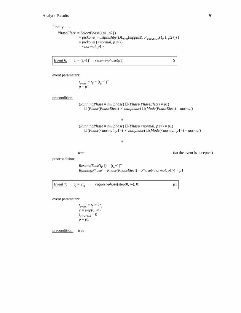
Analytic Results 91
Finally . . .
PhaseElect′ = SelectPhase({p1, p2})= pickone( mustfinishby(DL (mpplist), P ({p1, p2})) )first scheduled= pickone({<normal, p1>})= <normal, p1>
+Event 6: t = (t -1) resume-phase(p1) S6 a
event parameters:+t = t = (t −1)event 6 a
p = p1
precondition:
(RunningPhase = nullphase) ∧ (Phase(PhaseElect) = p1)∧ (Phase(PhaseElect) ≠ nullphase) ∧ (Mode(PhaseElect) = normal)
≡
(RunningPhase = nullphase) ∧ (Phase(<normal, p1>) = p1)∧ (Phase(<normal, p1>) ≠ nullphase) ∧ (Mode(<normal, p1>) = normal)
≡
true (so the event is accepted)
postconditions:+ResumeTime′(p1) = (t −1)a
RunningPhase′ = Phase(PhaseElect) = Phase(<normal, p1>) = p1
Event 7: t = 2t request-phase(step(0, ∞), 0) p17 a
event parameters:
t = t = 2tevent 7 av = step(0, ∞)t = 0expectedp = p1
precondition: true
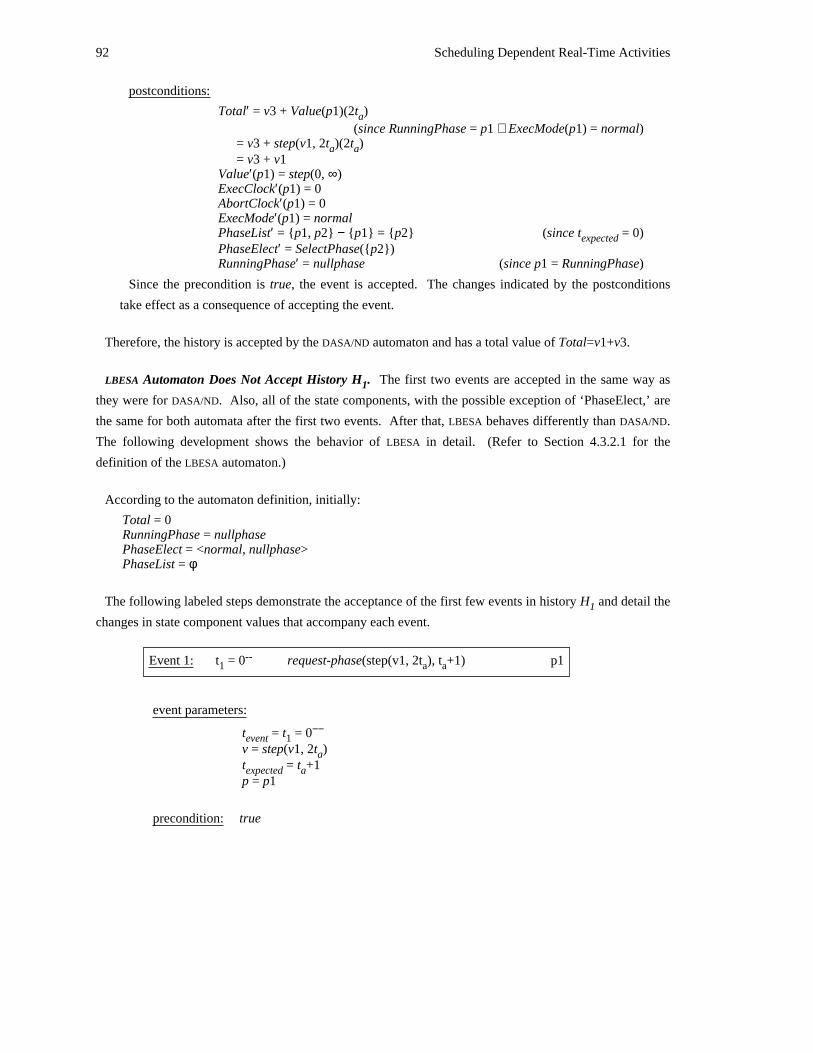
92 Scheduling Dependent Real-Time Activities
postconditions:
Total′ = v3 + Value(p1)(2t )a(since RunningPhase = p1 ∧ ExecMode(p1) = normal)
= v3 + step(v1, 2t )(2t )a a= v3 + v1
Value′(p1) = step(0, ∞)ExecClock′(p1) = 0AbortClock′(p1) = 0ExecMode′(p1) = normalPhaseList′ = {p1, p2} − {p1} = {p2} (since t = 0)expectedPhaseElect′ = SelectPhase({p2})RunningPhase′ = nullphase (since p1 = RunningPhase)
Since the precondition is true, the event is accepted. The changes indicated by the postconditions
take effect as a consequence of accepting the event.
Therefore, the history is accepted by the DASA/ND automaton and has a total value of Total=v1+v3.
LBESA Automaton Does Not Accept History H . The first two events are accepted in the same way as1
they were for DASA/ND. Also, all of the state components, with the possible exception of ‘PhaseElect,’ are
the same for both automata after the first two events. After that, LBESA behaves differently than DASA/ND.
The following development shows the behavior of LBESA in detail. (Refer to Section 4.3.2.1 for the
definition of the LBESA automaton.)
According to the automaton definition, initially:
Total = 0RunningPhase = nullphasePhaseElect = <normal, nullphase>PhaseList = φ
The following labeled steps demonstrate the acceptance of the first few events in history H and detail the1
changes in state component values that accompany each event.
--Event 1: t = 0 request-phase(step(v1, 2t ), t +1) p11 a a
event parameters:−−t = t = 0event 1
v = step(v1, 2t )at = t +1expected ap = p1
precondition: true
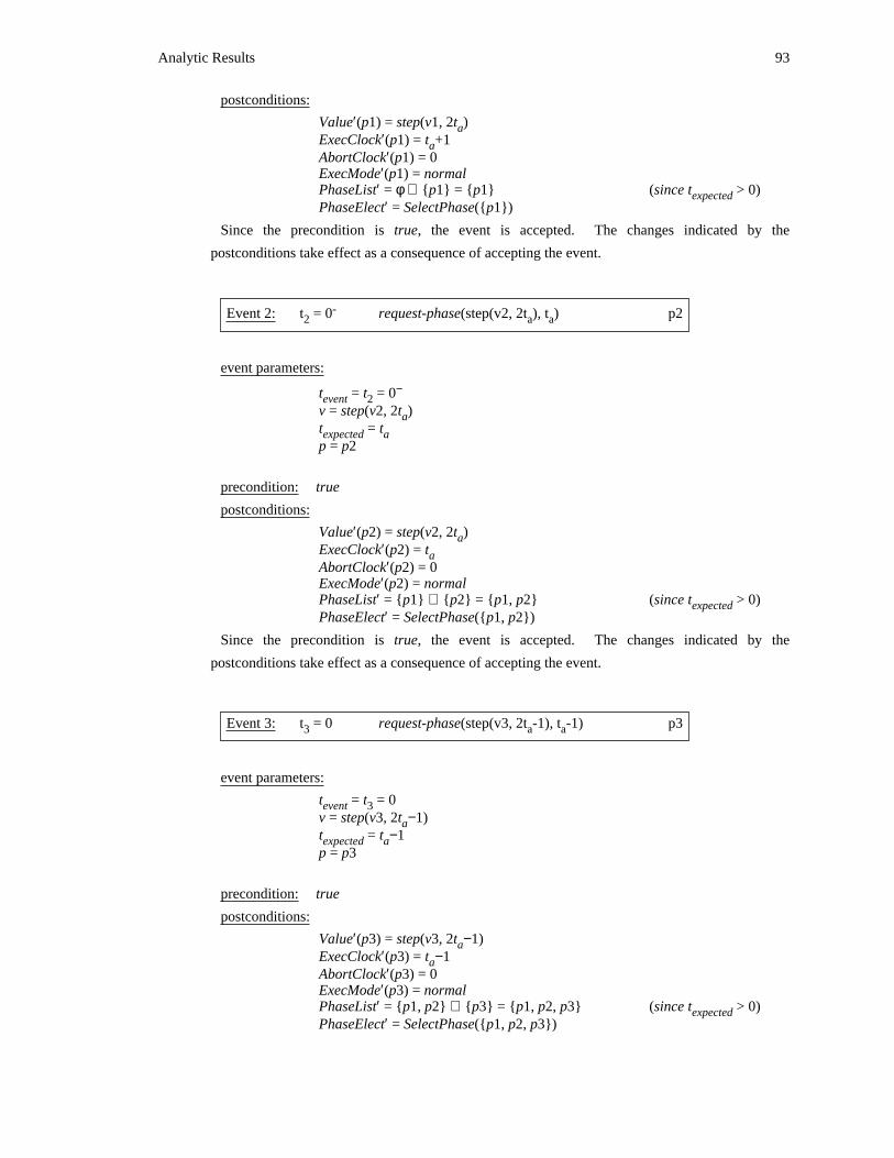
Analytic Results 93
postconditions:
Value′(p1) = step(v1, 2t )aExecClock′(p1) = t +1aAbortClock′(p1) = 0ExecMode′(p1) = normalPhaseList′ = φ ∪ {p1} = {p1} (since t > 0)expectedPhaseElect′ = SelectPhase({p1})
Since the precondition is true, the event is accepted. The changes indicated by the
postconditions take effect as a consequence of accepting the event.
-Event 2: t = 0 request-phase(step(v2, 2t ), t ) p22 a a
event parameters:−t = t = 0event 2
v = step(v2, 2t )at = texpected ap = p2
precondition: true
postconditions:
Value′(p2) = step(v2, 2t )aExecClock′(p2) = taAbortClock′(p2) = 0ExecMode′(p2) = normalPhaseList′ = {p1} ∪ {p2} = {p1, p2} (since t > 0)expectedPhaseElect′ = SelectPhase({p1, p2})
Since the precondition is true, the event is accepted. The changes indicated by the
postconditions take effect as a consequence of accepting the event.
Event 3: t = 0 request-phase(step(v3, 2t -1), t -1) p33 a a
event parameters:
t = t = 0event 3v = step(v3, 2t −1)at = t −1expected ap = p3
precondition: true
postconditions:
Value′(p3) = step(v3, 2t −1)aExecClock′(p3) = t −1aAbortClock′(p3) = 0ExecMode′(p3) = normalPhaseList′ = {p1, p2} ∪ {p3} = {p1, p2, p3} (since t > 0)expectedPhaseElect′ = SelectPhase({p1, p2, p3})
94 Scheduling Dependent Real-Time Activities
Since the precondition is true, the event is accepted. The changes indicated by the
postconditions take effect as a consequence of accepting the event.
Evaluating SelectPhase( {p1, p2, p3} ) . . .
SelectPhase( {p1, p2, p3} )= pickone( mustfinishby(DL (mpplist), P ({p1, p2, p3})) )first scheduled
where
mpplist = tobescheduled(P ({p1, p2, p3}))scheduled
P ({p1, p2, p3})scheduled= P (P ({p1, p3}) ∪ {p2})(since P ({p1, p2, p3}) = {p2})feasible scheduled lastDL
P ({p1, p3})scheduled= P (P ({p3}) ∪ {p1}) (since P ({p1, p3}) = {p1})feasible scheduled lastDL
P ({p3})scheduled= P (P (φ) ∪ {p3}) (since P ({p1}) = {p1})feasible scheduled lastDL= P (φ ∪ {p3})feasible= P ({p3})feasible= {p3}, if feasible({p3})
feasible({p3}) = true,iff (∀t)[(t ≥ t ) → timerequiredby(mustfinishby(t, {p3})) ≤ (t−t )]event event
For t ≥ t . . .event
mustfinishby(t, {p3})
φ, if mustcompleteby(t, {p3}) = φ={ {<normal, p> | p ∈ mustcompleteby(t, {p3})},otherwise
mustcompleteby(t, {p3})= {p | [p ∈ {p3} ∧ Deadline(p) ≤ t]}
φ, if t < Deadline(p3) = 2t −1= a{{p3}, if t ≥ Deadline(p3) = 2t −1a
Therefore . . .
mustfinishby(t, {p3})
φ, if t < 2t −1= a{{<normal, p> | p ∈ {p3}}, otherwise
φ, if t < 2t −1= a{ {<normal, p3>}, otherwise
timerequiredby(mustfinishby(t, {p3}))
timerequiredby(φ), if t < 2t −1= a{timerequiredby({<normal, p3>}), if t ≥ 2t −1a
0, if t < 2t −1= a{ExecClock(p3) = t −1, if t ≥ 2t −1a a
Analytic Results 95
Notice that for t ≥ t = 0, when t < 2t −1 . . .event a
timerequiredby(mustfinishby(t, {p3})) = 0 ≤ (t−t )event
as required for feasibility.
And when t ≥ 2t −1 . . .a
timerequiredby(mustfinishby(t, {p3})) = t −1 ≤ 2t −1 ≤ (t−t )a a event
as required for feasibility.
Therefore . . .
feasible({p3}) = true → P ({p3}) = {p3}scheduled
Continuing . . .
P ({p1, p3})scheduled= P (P ({p3}) ∪ {p1}) (as shown above)feasible scheduled= P ({p3} ∪ {p1})feasible= P ({p1, p3})feasible
feasible({p1, p3}) = true, iff (∀t)[(t ≥ t )event→ timerequiredby(mustfinishby(t, {p1, p3})) ≤ (t−t )]event
For t ≥ t . . .event
mustfinishby(t, {p1, p3})
φ, if mustcompleteby(t, {p1, p3}) = φ={[ {<normal, p> | p ∈ mustcompleteby(t, {p1, p3})},otherwise
mustcompleteby(t, {p1, p3})= {p | [p ∈ {p1, p3} ∧ Deadline(p) ≤ t]}
φ, if t < Deadline(p3) = 2t −1a{p3}, if Deadline(p3) = 2t −1 ≤ ta= < Deadline(p1) = 2t{ a{p1, p3}, if t ≥ Deadline(p1) = 2ta
Therefore . . .
mustfinishby(t, {p1, p3})
φ, if t < 2t −1a= {<normal, p> | p ∈ {p3}}, if 2t −1 ≤ t < 2ta a{
{<normal, p> | p ∈ {p1, p3}}, if 2t ≤ ta
φ, if t < 2t −1a= {<normal, p3>}, if 2t −1 ≤ t < 2ta a{
{<normal, p1>, <normal, p3>}, if 2t ≤ ta
96 Scheduling Dependent Real-Time Activities
timerequiredby(mustfinishby(t, {p1, p3}))
timerequiredby(φ), if t < 2t −1a= timerequiredby({<normal, p3>}), if 2t −1 ≤ t < 2ta a{
timerequiredby({<normal, p1>, <normal, p3>}),if 2t ≤ ta
0, if t < 2t −1a= ExecClock(p3) = t −1, if 2t −1 ≤ t < 2ta a a{
ExecClock(p1) + ExecClock(p3) = 2t ,aif 2t ≤ ta
Notice that for t ≥ t = 0, when t < 2t −1 . . .event a
timerequiredby(mustfinishby(t, {p1, p3})) = 0 ≤ (t−t )event
as required for feasibility.
When 2t −1 ≤ t < 2t . . .a a
timerequiredby(mustfinishby(t, {p1, p3})) = t −1 ≤ 2t −1 ≤ (t−t )a a event
as required for feasibility.
And when t ≥ 2t . . .a
timerequiredby(mustfinishby(t, {p1, p3})) = 2t ≤ (t−t )a event
as required for feasibility.
Therefore . . .
feasible({p1, p3}) = true→ P ({p1, p3}) = {p1, p3}feasible→ P ({p1, p3}) = {p1, p3}scheduled
Continuing . . .
P ({p1, p2, p3})scheduled= P (P ({p1, p3}) ∪ {p2}) (as shown above)feasible scheduled= P ({p1, p3} ∪ {p2})feasible= P ({p1, p2, p3})feasible
To evaluate P ({p1, p2, p3}) . . .feasible
feasible({p1, p2, p3}) = true, iff (∀t)[(t ≥ t )event→ timerequiredby(mustfinishby(t, {p1, p2, p3})) ≤ (t−t )]event
For t ≥ t . . .event
mustfinishby(t, {p1, p2, p3})
φ, if mustcompleteby(t, {p1, p2, p3}) = φ={ {<normal, p> | p ∈ mustcompleteby(t, {p1, p2, p3})},otherwise
mustcompleteby(t, {p1, p2, p3})= {p | [p ∈ {p1, p2, p3} ∧ Deadline(p) ≤ t]}
φ, if t < Deadline(p3) = 2t −1a{p3}, if Deadline(p3) = 2t −1 ≤ ta= < Deadline(p1) = 2t{ a{p1, p2, p3}, if t ≥ Deadline(p1) = 2ta
Analytic Results 97
Therefore . . .
mustfinishby(t, {p1, p2, p3})
φ, if t < 2t −1a= {<normal, p> | p ∈ {p3}}, if 2t −1 ≤ t < 2ta a{
{<normal, p> | p ∈ {p1, p2, p3}}, if 2t ≤ ta
φ, if t < 2t −1a= {<normal, p3>}, if 2t −1 ≤ t < 2ta a{
{<normal, p1>, <normal, p2>, <normal, p3>},if 2t ≤ ta
timerequiredby(mustfinishby(t, {p1, p2, p3}))
timerequiredby(φ), if t < 2t −1a= timerequiredby({<normal, p3>}), if 2t −1 ≤ t < 2ta a{
timerequiredby({<normal, p1>, <normal, p2>, <normal, p3>}),if 2t ≤ ta
0, if t < 2t −1a= ExecClock(p3) = t −1, if 2t −1 ≤ t < 2ta a a{
ExecClock(p1) + ExecClock(p2) + ExecClock(p3) = 3t ,aif 2t ≤ ta
Notice that for t = 2t . . .a
timerequiredby(mustfinishby(t, {p1, p2, p3})) = 3t > 2t = (t−t )a a event
This violates the requirement for feasibility. Therefore . . .
feasible({p1, p2, p3}) = false→ P ({p1, p2, p3}) = P ({p1, p2})feasible feasible
(since P ({p1, p2, p3}) = {p3})leastPV
To evaluate P ({p1, p2}) . . .feasible
feasible({p1, p2}) = true, iff (∀t)[(t ≥ t )event→ timerequiredby(mustfinishby(t, {p1, p2})) ≤ (t−t )]event
For t ≥ t . . .event
mustfinishby(t, {p1, p2})
φ, if mustcompleteby(t, {p1, p2}) = φ={ {<normal, p> | p ∈ mustcompleteby(t, {p1, p2})},otherwise
mustcompleteby(t, {p1, p2})= {p | [p ∈ {p1, p2} ∧ Deadline(p) ≤ t]}
φ, if t < Deadline(p1) = Deadline(p2) = 2t= a{{p1, p2}, if t ≥ Deadline(p1) = Deadline(p2) = 2ta
98 Scheduling Dependent Real-Time Activities
Therefore . . .
mustfinishby(t, {p1, p2})
φ, if t < 2t= a{{<normal, p> | p ∈ {p1, p2}}, otherwise
φ, if t < 2t= a{ {<normal, p1>, <normal, p2>}, otherwise
timerequiredby(mustfinishby(t, {p1, p2}))
timerequiredby(φ), if t < 2t= a{ timerequiredby({<normal, p1>, <normal, p2>}),if t ≥ 2ta
0, if t < 2t= a{ ExecClock(p1) + ExecClock(p2) = 2t +1,aif t ≥ 2ta
Notice that for t = 2t . . .a
timerequiredby(mustfinishby(t, {p1, p2})) = 2t +1 > 2t = (t−t )a a event
This violates the requirement for feasibility. Therefore . . .
feasible({p1, p2}) = false→ P ({p1, p2}) = P ({p1}) (since P ({p1, p2}) = {p2})feasible feasible leastPV
To evaluate P ({p1}) . . .feasible
feasible({p1}) = true,iff (∀t)[(t ≥ t ) → timerequiredby(mustfinishby(t, {p1})) ≤ (t−t )]event event
For t ≥ t . . .event
mustfinishby(t, {p1})
φ, if mustcompleteby(t, {p1}) = φ={ {<normal, p> | p ∈ mustcompleteby(t, {p1})},otherwise
mustcompleteby(t, {p1})= {p | [p ∈ {p1} ∧ Deadline(p) ≤ t]}
φ, if t < Deadline(p1) = 2t= a{{p1}, if t ≥ Deadline(p1) = 2ta
Therefore . . .
mustfinishby(t, {p1})
φ, if t < 2t= a{{<normal, p> | p ∈ {p1}}, otherwise
φ, if t < 2t= a{ {<normal, p1>}, otherwise
timerequiredby(mustfinishby(t, {p1}))
timerequiredby(φ), if t < 2t= a{timerequiredby({<normal, p1>}), if t ≥ 2ta
0, if t < 2t= a{ExecClock(p1) = t +1, if t ≥ 2ta a
Analytic Results 99
Notice that for t ≥ t = 0, when t < 2t . . .event a
timerequiredby(mustfinishby(t, {p1})) = 0 ≤ (t−t )event
as required for feasibility.
And when t ≥ 2t . . .a
timerequiredby(mustfinishby(t, {p1})) = t +1 ≤ 2t ≤ (t−t )a a event
as required for feasibility.
Therefore . . .
feasible({p1}) = true → P ({p1}) = {p1}feasible
Putting this together . . .
P ({p1, p2, p3}) = P ({p1, p2, p3})scheduled feasible= P ({p1, p2})feasible
(since feasible({p1, p2, p3}) = false ∧ P ({p1, p2, p3}) = {p3})leastPV= P ({p1})feasible
(since feasible({p1, p2}) = false ∧ P ({p1, p2}) = {p2})leastPV= {p1} (as shown above)
At this point, the set of phases that can be feasibly executed has been determined. Now to
decide which phase to be executed first . . .
mpplist = tobescheduled(P ({p1, p2, p3}))scheduled= tobescheduled({p1})= {<normal, p1>}
DL (mpplist) = DL ({<normal, p1>})first first= 2ta
mustfinishby(DL (mpplist), P ({p1, p2, p3}))first scheduled= mustfinishby(2t , {p1})a= {<normal, p> | p ∈ mustcompleteby(2t , {p1})}a
(assuming mustcompleteby(2t , {p1}) ≠ φ)a= {<normal, p> | p ∈ {q | [q ∈ {p1} ∧ Deadline(q) ≤ 2t ]}}a= {<normal, p> | p ∈ {p1}} (note that mustcompleteby(2t , {p1}) ≠ φ)a= {<normal, p1>}
Finally . . .
PhaseElect′ = SelectPhase({p1, p2, p3})= pickone( mustfinishby(DL (mpplist), P ({p1, p2, p3})) )first scheduled= pickone({<normal, p1>})= <normal, p1>
+Event 4: t = 0 resume-phase(p3) S4
event parameters:+t = t = 0event 4
p = p3
100 Scheduling Dependent Real-Time Activities
precondition:
(RunningPhase = nullphase) ∧ (Phase(PhaseElect) = p3)∧ (Phase(PhaseElect) ≠ nullphase) ∧ (Mode(PhaseElect) = normal)
≡
(RunningPhase = nullphase) ∧ (Phase(<normal, p1>) = p3)∧ (Phase(<normal, p1>) ≠ nullphase) ∧ (Mode(<normal, p1>) = normal)
≡
(RunningPhase = nullphase) ∧ (p1 = p3)∧ (p1 ≠ nullphase) ∧ (normal = normal)
≡
false, (since p1 ≠ p3)
Since the precondition is not satisfied, the event cannot be accepted.
Therefore, history H is not accepted by the LBESA automaton.1
LBESA cannot accept any history that begins with Events (1)-(3) and that has only those three phases,
with the already specified time-value functions and computation time requirements, that will yield a total
value greater than v1.
This proof will be carried out by identifying all of the histories that LBESA can accept under these
circumstances. The total value resulting from each of these histories will then be examined to demonstrate
that none is greater than v1.
To begin to identify the histories that are accepted by LBESA, notice that, given Events (1)-(3), LBESA will
behave exactly as described in the preceding analysis. Therefore, after accepting Event (3), the third event
in this sequence, the only events whose preconditions are satisfied are:1. any ‘request-phase’
2. ‘resume-phase(p1)’
Examine the first possibility −− any ‘request-phase’ event −− more closely. Let p denote the phasex
originating a ‘request-phase’ event. If p ∉ {p1, p2, p3}, then p is a new phase. But this violates thex x
assertion that the only histories being considered consist solely of events associated with phases p1, p2, and
p3. Therefore, p must be a member of {p1, p2, p3}.x
Also, notice that after accepting Events (1)-(3), RunningPhase = nullphase, which is not a member of
{p1, p2, p3}. Consequently, the postconditions of the event ‘request-phase(v , t ) p ’ are:x x x
Analytic Results 101
Value′(p ) = vx xExecClock′(p ) = tx xAbortClock′(p ) = 0xExecMode′(p ) = normalxPhaseList′ = PhaseList ∪ {p } or PhaseList − {p }x xPhaseElect′ = SelectPhase(PhaseList′)
These postconditions serve only to alter or reiterate the scheduling parameters of the already defined
phases (possibly removing one of the phases from consideration from scheduling at the same time and
potentially selecting a new PhaseElect to reflect these changes). If the scheduling parameters are altered,
this violates the assertion that the automaton will consider only the time-value functions and expected
computation times already specified for the three phases by the first three events. Consequently, the only
‘request-phase’ events that LBESA can accept at this point reiterate the scheduling parameters for p ∈ {p1,x
p2, p3}. (Hereafter, ‘request-phase’ events that serve to reiterate previously defined scheduling parameters
may be referred to as reiterative ‘request-phase’ events.) Furthermore, notice that although such
‘request-phase’ events do not alter the scheduling parameters for a phase −− they merely reiterate them −−there is a potential effect of these events on the automaton state component PhaseElect, which is set equal
to SelectPhase(PhaseList′) as a postcondition of each ‘request-phase’ event. The function SelectPhase() is
dependent on t , which increases during the course of any history.event
To examine the effect of a ‘request-phase’ on PhaseElect consider first the effect on the value of
P ({p1, p2, p3}) as a function of t . Of course, t > 0 since only legal histories are underscheduled event event
consideration here, and the third event occurred at time t = 0. With that in mind, expand the value of2
P ({p1, p2, p3}) as follows:scheduled
P ({p1, p2, p3}) = P (P ({p1, p3}) ∪ {p2})scheduled feasible scheduled(since P ({p1, p2, p3}) = {p2})lastDL
= P (P (P ({p3}) ∪ {p1}) ∪ {p2})feasible feasible scheduled(since P ({p1, p3}) = {p1})lastDL
= P (P (P (P (φ) ∪ {p3}) ∪ {p1}) ∪ {p2})feasible feasible feasible scheduled(since P ({p3}) = {p3})lastDL
= P (P (P (φ ∪ {p3}) ∪ {p1}) ∪ {p2})feasible feasible feasible= P (P (P ({p3}) ∪ {p1}) ∪ {p2})feasible feasible feasible
{p3}, if feasible({p3})P ({p3}) =feasible { φ, otherwise
Several feasibility conditions like this will have to be evaluated in the following section of the proof.
Therefore, a general result will be derived here that can be applied to any of the simple cases that follow.
Consider a phase p with automaton state components:
Value(p) = step(v, t )DLExecClock(p) = trequiredAbortClock(p) = 0ExecMode(p) = normal
Notice that p1, p2, and p3 all satisfy this profile at this point in the automaton’s examination of any
history that it accepts. Then . . .
feasible({p}) = true, iff (∀t)[(t ≥ t ) → timerequiredby(mustfinishby(t, {p})) ≤ (t−t )]event event
102 Scheduling Dependent Real-Time Activities
For t ≥ t . . .event
timerequiredby(mustfinishby(t, {p}))
timerequiredby(φ), if mustcompleteby(t, {p}) = φ={ timerequiredby({<normal, q> | q ∈ mustcompleteby(t, {p})}),otherwise
mustcompleteby(t, {p}) = {q | [q ∈ {p} ∧ Deadline(q) ≤ t]}
φ, if t < t= DL{{p}, if t ≥ tDL
Therefore,
timerequiredby(mustfinishby(t, {p}))
timerequiredby(φ), if t < t= DL{timerequiredby({<normal, p>}), if t ≥ tDL
0, if t < t= DL{ExecClock(p), if t ≥ tDL
If feasible({p}) = true, then, by definition, for any t ≥ t . . .event
timerequiredby(mustfinishby(t, {p})) ≤ (t−t )event
For the cases where t < t , this relation is trivially satisfied since the left-hand side of the relation isDL
equal to zero and the right-hand side is greater than or equal to zero by definition
(t ≥ t → (t − t ) ≥ 0). For the cases where t ≥ t . . .event event DL
ExecClock(p) ≤ t−tevent→ t ≤ t−ExecClock(p)event
Applying this general result to each of the three phases under consideration when (a)
ExecClock(p) = t −− that is, the phase has not yet begun to execute −− and (b) t = t yields:required DL
• feasible({p1}) = true, iff t ≤ 2t −(t +1) = t −1event a a a
• feasible({p2}) = true, iff t ≤ 2t −t = tevent a a a
• feasible({p3}) = true, iff t ≤ (2t −1) − (t −1) = tevent a a a
Using this information in the previously derived expression for P ({p3}) yields . . .feasible
P ({p3})feasible
{p3}, if feasible({p3})={ φ, otherwise
{p3}, if 0 ≤ t ≤ t= event a{ φ, if t < ta event
P ({p1, p2, p3})scheduled
P (P ({p3} ∪ {p1}) ∪ {p2}), if 0 ≤ t ≤ t= feasible feasible event a{P (P (φ ∪ {p1}) ∪ {p2}), if t < tfeasible feasible a event
P (P ({p1,p3}) ∪ {p2}), if 0 ≤ t ≤ t= feasible feasible event a{P (P ({p1}) ∪ {p2}), if t < tfeasible feasible a event
Analytic Results 103
For t < t . . .a event
P ({p1, p2, p3})scheduled= P (P ({p1}) ∪ {p2})feasible feasible= P (φ ∪ {p2}) (since feasible({p1}) = false for t < t )feasible a event= P ({p2})feasible= φ (since feasible({p2}) = false for t < t )a event
Consider the other case in the derivation of P ({p1, p2, p3}), where 0 ≤ t ≤ t . . .scheduled event a
P ({p1, p2, p3})scheduled= P (P ({p1, p3}) ∪ {p2})feasible feasible
P ({p1, p3} ∪ {p2}), if t = 0feasible event= (since P ({p1, p3}) = {p1, p3})feasible{
P (P ({p1}) ∪ {p2}), if 0 < t ≤ tfeasible feasible event a(since P ({p1, p3}) = P ({p1}))feasible feasible
P ({p1, p2, p3}), if t = 0feasible eventP ({p1} ∪ {p2}), if 0 < t ≤ t −1feasible event a
= (since feasible({p1}) = true iff t ≤ t −1){ event aP (φ ∪ {p2}), if t −1 < t ≤ tfeasible a event a
P ({p1, p2, p3}), if t = 0feasible event= P ({p1, p2}), if 0 < t ≤ t −1feasible event a{
P ({p2}), if t −1 < t ≤ tfeasible a event a
P ({p1, p2, p3}), if t = 0feasible eventP ({p1}), if 0 < t ≤ t −1feasible event a= (since P ({p1, p2}) = P ({p1})){ feasible feasibleP ({p2}), if t −1 < t ≤ tfeasible a event a
{p1}, if t = 0 (as shown previously)event{p1}, if 0 < t ≤ t −1event a
= (since feasible({p1}) = true iff t ≤ t −1){ event a{p2}, if t −1 < t ≤ ta event a
(since feasible({p2}) = true iff t ≤ t )event a
Putting it all together . . .
P ({p1, p2, p3})scheduled
{p1}, if 0 ≤ t ≤ t −1event a= {p2}, if t −1 < t ≤ ta event a{φ, if t < ta event
Remember that, by definition:
SelectPhase({p1, p2, p3}) = pickone( mustfinishby(DL (mpplist), P ({p1, p2, p3})) )first scheduled
where
mpplist = tobescheduled(P ({p1, p2, p3}))scheduled
104 Scheduling Dependent Real-Time Activities
As a consequence of these last two facts:
SelectPhase({p1, p2, p3})
<normal, p1>, if 0 ≤ t ≤ t −1event a= <normal, p2>, if t −1 < t ≤ ta event a{
<normal, nullphase>, if t < ta event
The outcome of this portion of the analysis is that any number of ‘request-phase’ events can occur to
reiterate scheduling parameters of the three phases of concern. These events will be accepted by the LBESA
automaton and the PhaseElect state component will have its value changed as indicated above for
PhaseElect = SelectPhase({p1, p2, p3}). The (possibly empty) sequence of scheduling parameter
reiterations may be terminated by a ‘resume-phase’ event for phase PhaseElect at any time.
This ‘resume-phase’ event may be followed by any number of reiterative ‘request-phase’ events for the
two phases that are not executing. Once again, these ‘request-phase’ events may change the value of the35PhaseElect state component . However, the value of PhaseElect as a function of t will still be theevent
same as was concluded by the preceding analysis.
Although the SelectPhase() evaluation yields the same value as a function of t as before, there is oneevent
additional consideration that was not present earlier: that is, once a phase has begun execution, its
ExecClock state component is updated each time a ‘request-phase’ event is accepted. Specifically, the
ExecClock state component is decreased, resulting in an increase in that phase’s PVD() metric. This
increase does not change the outcome of the scheduling decision because only the executing phase’s
potential value density changes and:1. if phase p1 is executing, its PVD() was already higher than those of the other two phases, so
any further increase makes no difference in the rankings used by LBESA, which only considerwhether one PVD() is larger than another, not how much larger.
2. if phase p2 is executing, its PVD() could exceed that of p1. The earlier analysis indicated thatp2 could only execute when p1 could no longer feasibly execute. In fact, if p1 completesexecution successfully, it is impossible to complete p2. Therefore, the fact that p2 is everable to begin execution indicates that p1 did not, and cannot, successfully completeexecution.
Whenever a scheduling decision is made after p2 has begun execution, p3 will first beconsidered for inclusion in a tentative schedule since it has the nearest deadline. Ifcompleting p3 is not feasible −− and completing p1 is not feasible −− then only p2 canpossibly complete and contribute value to the accepted history. If, on the other hand, p3 canfeasibly complete, then the other two phases are considered for inclusion into the tentativeschedule, with the phase with the higher PVD() considered first. If the PVD() of p2 doessurpass that of p1, the order in which they are considered will change. However, since p1cannot be scheduled feasibly, it will trigger the elimination of (at least) the phase with thelowest PVD() from the schedule. This is p3, and it will be eliminated no matter if p1precedes or follows p2.
Since it is difficult to follow a narrative description of all of the potential histories that may be accepted
35In fact, the first ‘request-phase’ event occurring after the ‘resume-phase’ may cause a change in value in PhaseElect, thuspotentially triggering a preemption. This will be explained shortly.
Analytic Results 105
36by LBESA, the following approach is taken . Consider the diagram shown in Figure 4-9, where each+ *labeled item is an event, "E " indicates one or more occurrences of the expression "E", and "E " indicates
zero or more occurrences of the expression "E". (The labels "(Case X)" are merely used in the ensuing
discussion to refer to specific branches of the diagram.)
To use the diagram to trace an individual history accepted by LBESA, begin with the first event, E , which1
appears on the top line, and proceed down one line at a time. Each line may add events to the history.
Where there are branches, choose one path or the other and continue to move down through the diagram.37The history may be terminated at any time
To demonstrate that the diagram is correct, that is, that it incorporates all of the legal histories that LBESA
will accept, consider the following.
As was discussed earlier, a ‘request-phase’ event may be accepted at any time, as long as it serves only to
reiterate the already established scheduling parameters for a phase. As a result, the diagram indicates that*such events, labeled [E ] , may occur between any other two events in a history.reiterate
As was also shown earlier, an examination of the preconditions of the various potential events indicates
that the only event that may be accepted after E , E , E , and any other reiterative ‘request-phase’ events is1 2 3
a ‘resume-phase’ event to start the execution of the phase that is currently designated PhaseElect (as long
as PhaseElect is not the nullphase). Hence, E can only be a ‘resume-phase’ event.4
There are two possible courses that may be followed after E : (a) the phase may be preempted (Case I) or4
(b) it may complete execution (Case II). In the latter case, if the phase runs to completion, then it will
originate a ‘request-phase’ event to signal that circumstance. This event will always be accepted because
its precondition is simply true. In Case I, examination of the precondition for a ‘preempt-phase’ event
indicates that a preemption can only occur if RunningPhase is not the same as PhaseElect and is not the
nullphase. The postconditions of event E guarantee that RunningPhase is not the nullphase. Hence, if a4
‘request-phase’ event following E yielded a value of PhaseElect different from RunningPhase, then,4
according to the previous analysis of SelectPhase({p1, p2, p3}), the only possibilities are:1. E resumed p1, and PhaseElect subsequently becomes either p2 or nullphase, or4
2. E resumed p2, and PhaseElect subsequently becomes the nullphase4
Currently, the assumption is made that the required computation time for a phase is known exactly.
Whenever the phase designated by PhaseElect is resumed immediately after a ‘request-phase’ event, it will
be able to meet its deadline if it runs uninterrupted because a test of feasibility was carried out that verified
exactly that fact. However, if time is allowed to elapse between the ‘request-phase’ and the
36In examining all possible histories that LBESA will accept, a number of histories that would seem to be nonsense are considered.They are artifacts of the formal model, rather than indications of anticipated scheduler behavior. In all likelihood, any actual LBESA
implementation, when scheduling this collection of computational phases, would run p1 as soon as possible (that is, at time 0).Neither of the other phases would ever execute.
37At any time after the third event, that is. By definition, the only histories being considered are those that begin with events E , E ,1 2and E , in that order.3
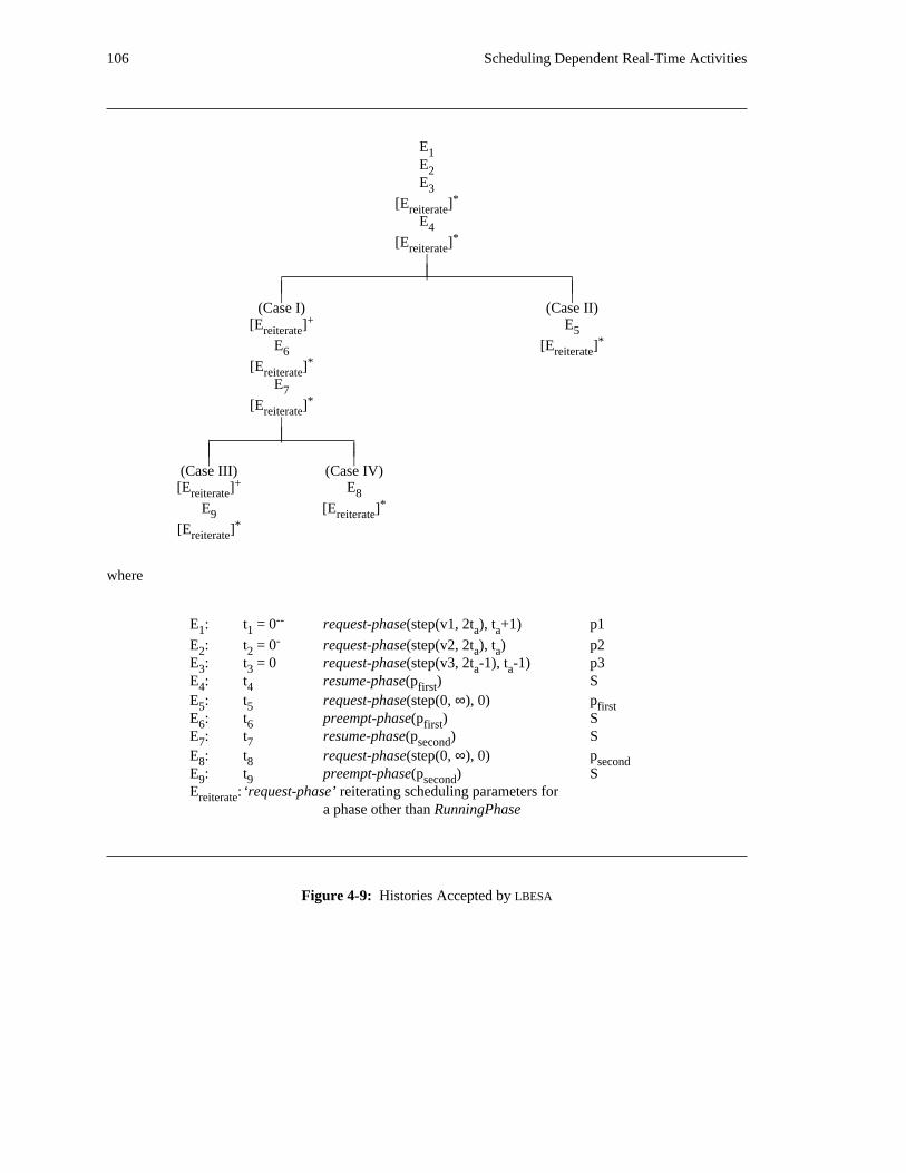
106 Scheduling Dependent Real-Time Activities
E1E2E3
*[E ]reiterateE4
*[E ]reiterate|||
| || || |
(Case I) (Case II)+[E ] Ereiterate 5
*E [E ]6 reiterate*[E ]reiterate
E7*[E ]reiterate
|||
| || || |
(Case III) (Case IV)+[E ] Ereiterate 8
*E [E ]9 reiterate*[E ]reiterate
where
--E : t = 0 request-phase(step(v1, 2t ), t +1) p11 1 a a-E : t = 0 request-phase(step(v2, 2t ), t ) p22 2 a a
E : t = 0 request-phase(step(v3, 2t -1), t -1) p33 3 a aE : t resume-phase(p ) S4 4 firstE : t request-phase(step(0, ∞), 0) p5 5 firstE : t preempt-phase(p ) S6 6 firstE : t resume-phase(p ) S7 7 secondE : t request-phase(step(0, ∞), 0) p8 8 secondE : t preempt-phase(p ) S9 9 secondE :‘request-phase’ reiterating scheduling parameters forreiterate
a phase other than RunningPhase
Figure 4-9: Histories Accepted by LBESA
Analytic Results 107
‘resume-phase’ events, it is possible that it is no longer feasible to execute PhaseElect by the time it is38actually initiated . Subsequent ‘request-phase’ events serve to indicate that fact by selecting a PhaseElect
other than RunningPhase, thereby setting the stage for a preemption.
Consider the next non-‘request-phase’ event to be accepted by LBESA under Case II in the diagram. If the
first phase to execute, p , completes execution, it signals this fact by originating event E . Then thefirst 5
subsequent evaluation of either PhaseElect = SelectPhase({p2, p3}) (in the case where p was p1) orfirst
PhaseElect = SelectPhase({p1, p3}) (in the case where p was p2) yieldsfirst
PhaseElect = <normal, nullphase>. Therefore, no subsequent ‘resume-phase’ event can be accepted by the
automaton since the necessary precondition cannot be satisfied. Also, since RunningPhase = nullphase
following E , no new ‘preempt-phase’ event can be accepted either. So, except for reiterative5
‘request-phase’ events, no further events can be accepted in these particular histories.
In Case I, where the first phase to execute was preempted, this fact was indicated by event E . As one of6
its postconditions, E set RunningPhase = nullphase. The next event in any history accepted by LBESA,6
other than reiterative ‘request-phase’ events, cannot be another ‘preempt-phase’ event because that would
require RunningPhase ≠ nullphase. Therefore, if any event other than a reiterative ‘request-phase’ event is
to be accepted by LBESA, it must be a ‘resume-phase’. In order to have such an event occur, PhaseElect
must, as a precondition, be non-nullphase. This can result from a reiterative ‘request-phase’ event
according to an analysis similar to the one done above.
Finally, if E , a ‘resume-phase’ event, is accepted in a history, then the situation and analysis is almost7
identical to the one that was examined after event E , the previous ‘resume-phase’. Once again, the4
resumed phase, p in this case, can either be preempted (Case III) or run to completion (Case IV), andsecond
the circumstances for each of these outcomes is exactly analogous to those given earlier for E . However,4
the earlier examination of SelectPhase({p1, p2, p3}) shows that there is no possible successor phase to
execute following either E or E . In both cases, this is due to the fact that p must be p2 and8 9 second
PhaseElect = SelectPhase({p1, p2, p3}) and PhaseElect = SelectPhase({p1, p3}) both yield
PhaseElect = <normal, nullphase>, which will not permit a subsequent ‘resume-phase’ event to be
accepted by LBESA.
While the above arguments demonstrate that the earlier diagram incorporates all of the legal histories that
may be accepted by LBESA, they do not reveal all of the factors involved in making the histories acceptable.
In particular, there are constraints on the times at which certain events occur, above and beyond those that
apply to any legal history, that must be satisfied to obtain certain histories. For instance, depending on the
timing of events, there is the possibility of executing zero, one, or two phases during the course of a history.
The following list specifies the time constraints that must be satisfied by various events to obtain given
histories:
38Intuitively, this can be thought of as reflecting a latency issue. In effect, the scheduler determines what can be feasibly completedin the available time from the instant at which a scheduling decision is made. However, if the latency encountered in actuallydispatching the next phase is large enough, then, by the time it has dispatched the phase, the set of phases that is feasible has changed.Notice that it is possible to specify this latency and apply certain restrictions to histories in order to model and accommodate thelatency. Also, it is possible to alter the algorithm embedded in the automaton to handle this latency when it is determining PhaseElect.In fact, this is done for DASA in the simulation experiments reported in Sections 5.3 and 5.4.
108 Scheduling Dependent Real-Time Activities
1. If the history includes event E , then p may be either p1 or p2; if it is to be p1, then t4 first eventfor the ‘request-phase’ immediately preceding E must satisfy:4
0 ≤ t ≤ t −1event a
If p is to be p2, then t for the ‘request-phase’ immediately preceding E must satisfy:first event 4
t −1 < t ≤ ta event a
2. If the history includes event E (Case I), then either:6a. p = p1 −− in this case, t , the time at event which E occurred, must have satisfied:first 4 4
t −1 < ta 4
b. p = p2 −− in this case, t , the time at event which E occurred, must have satisfied:first 4 4
t < ta 4393. If the history includes event E (Case II), then either :5
a. p = p1 −− in this case, t , the time at event which E occurs, must satisfy:first 5 5
t = t + (t +1)5 4 a
since required computation time is known accurately.
b. p = p2 −− in this case, t , the time at event which E occurs, must satisfy:first 5 5
t = t + t5 4 a
since required computation time is known accurately.
4. If the history includes event E , then p must be p1 and p must be p2. In addition,7 first secondt for the ‘request-phase’ immediately preceding E7 must satisfy:event
t −1 < t ≤ ta event a
5. If the history includes event E (Case IV), then t , the time at event which E occurs, must8 8 840satisfy :
t = t + t8 7 a
since required computation time is known accurately.
6. If the history includes event E (Case III), then, since p = p2, t , the time at event which E9 first 7 7occurred, must have satisfied:
t < ta 7
Once all of the histories that are accepted by LBESA have been enumerated, their respective values can
also be enumerated. To that end, the table shown in Figure 4-10 puts all of the preceding pieces of the
argument together. It lists all of the histories accepted by LBESA that start with events E , E , and E , along1 2 3
with their corresponding values.
39This is actually a requirement of any legal history. It is explicitly listed here since it does point out an important time constraintfor the history that otherwise might be forgotten.
40Once again, this is actually a requirement of any legal history and is only included here for the sake of completeness.
41The value at this point will be: (a) v1, if p = p1 and t ≤ t -1, (b) v2, if p = p2 and t ≤ t , or (c) 0, in all other cases.first 4 a first 4 a
42Same conditions as in the previous case determine the actual value.
43The value at this point will be: (a) v2, if t ≤ t , or (b) 0, otherwise.7 a
44Same conditions as in the previous case determine the actual value.
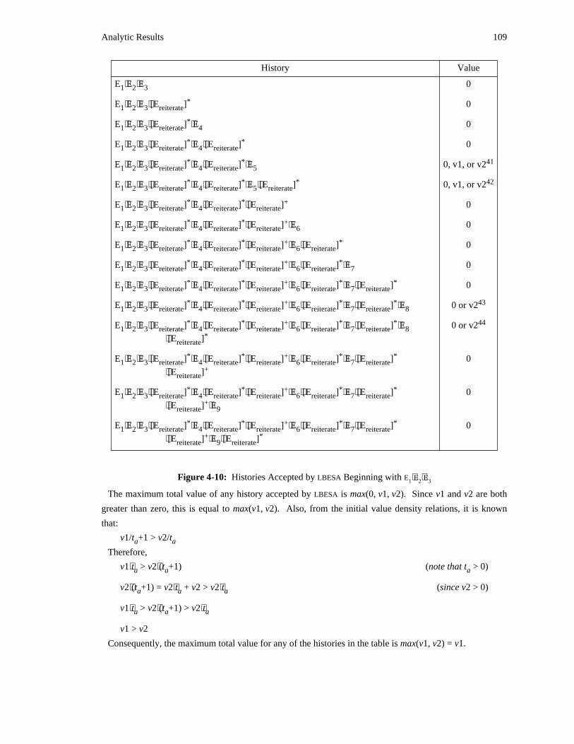
Analytic Results 109
History Value
E ⋅E ⋅E 01 2 3
*E ⋅E ⋅E ⋅[E ] 01 2 3 reiterate
*E ⋅E ⋅E ⋅[E ] ⋅E 01 2 3 reiterate 4
* *E ⋅E ⋅E ⋅[E ] ⋅E ⋅[E ] 01 2 3 reiterate 4 reiterate
* * 41E ⋅E ⋅E ⋅[E ] ⋅E ⋅[E ] ⋅E 0, v1, or v21 2 3 reiterate 4 reiterate 5
* * * 42E ⋅E ⋅E ⋅[E ] ⋅E ⋅[E ] ⋅E ⋅[E ] 0, v1, or v21 2 3 reiterate 4 reiterate 5 reiterate
* * +E ⋅E ⋅E ⋅[E ] ⋅E ⋅[E ] ⋅[E ] 01 2 3 reiterate 4 reiterate reiterate
* * +E ⋅E ⋅E ⋅[E ] ⋅E ⋅[E ] ⋅[E ] ⋅E 01 2 3 reiterate 4 reiterate reiterate 6
* * + *E ⋅E ⋅E ⋅[E ] ⋅E ⋅[E ] ⋅[E ] ⋅E ⋅[E ] 01 2 3 reiterate 4 reiterate reiterate 6 reiterate
* * + *E ⋅E ⋅E ⋅[E ] ⋅E ⋅[E ] ⋅[E ] ⋅E ⋅[E ] ⋅E 01 2 3 reiterate 4 reiterate reiterate 6 reiterate 7
* * + * *E ⋅E ⋅E ⋅[E ] ⋅E ⋅[E ] ⋅[E ] ⋅E ⋅[E ] ⋅E ⋅[E ] 01 2 3 reiterate 4 reiterate reiterate 6 reiterate 7 reiterate
* * + * * 43E ⋅E ⋅E ⋅[E ] ⋅E ⋅[E ] ⋅[E ] ⋅E ⋅[E ] ⋅E ⋅[E ] ⋅E 0 or v21 2 3 reiterate 4 reiterate reiterate 6 reiterate 7 reiterate 8
* * + * * 44E ⋅E ⋅E ⋅[E ] ⋅E ⋅[E ] ⋅[E ] ⋅E ⋅[E ] ⋅E ⋅[E ] ⋅E 0 or v21 2 3 reiterate 4 reiterate reiterate 6 reiterate 7 reiterate 8*⋅[E ]reiterate
* * + * *E ⋅E ⋅E ⋅[E ] ⋅E ⋅[E ] ⋅[E ] ⋅E ⋅[E ] ⋅E ⋅[E ] 01 2 3 reiterate 4 reiterate reiterate 6 reiterate 7 reiterate+⋅[E ]reiterate
* * + * *E ⋅E ⋅E ⋅[E ] ⋅E ⋅[E ] ⋅[E ] ⋅E ⋅[E ] ⋅E ⋅[E ] 01 2 3 reiterate 4 reiterate reiterate 6 reiterate 7 reiterate+⋅[E ] ⋅Ereiterate 9
* * + * *E ⋅E ⋅E ⋅[E ] ⋅E ⋅[E ] ⋅[E ] ⋅E ⋅[E ] ⋅E ⋅[E ] 01 2 3 reiterate 4 reiterate reiterate 6 reiterate 7 reiterate+ *⋅[E ] ⋅E ⋅[E ]reiterate 9 reiterate
Figure 4-10: Histories Accepted by LBESA Beginning with E ⋅E ⋅E1 2 3
The maximum total value of any history accepted by LBESA is max(0, v1, v2). Since v1 and v2 are both
greater than zero, this is equal to max(v1, v2). Also, from the initial value density relations, it is known
that:
v1/t +1 > v2/ta a
Therefore,
v1⋅t > v2⋅(t +1) (note that t > 0)a a a
v2⋅(t +1) = v2⋅t + v2 > v2⋅t (since v2 > 0)a a a
v1⋅t > v2⋅(t +1) > v2⋅ta a a
v1 > v2
Consequently, the maximum total value for any of the histories in the table is max(v1, v2) = v1.
110 Scheduling Dependent Real-Time Activities
As shown in the first section of this proof, DASA/ND accepts a history with value (v1+v3) starting with
these three events, while the maximum value for a history accepted by LBESA is v1. Therefore, there exists
a case in which DASA/ND accepts a history with greater value than LBESA, and there is no transformation of
that history or alternate history dealing with the same phases and scheduling parameters that allows LBESA
to obtain an equal or greater value than DASA/ND.
EndOfProof
Since the DASA/ND Scheduling Automaton is equivalent to the DASA Scheduling Automaton when there
are no dependency considerations, the result extends to the DASA Scheduling Automaton as well.
4.3.3. Algorithm Tractability
This section examines the computational complexity of the DASA scheduling algorithm. Specifically, the
amount of time and space required for the DASA algorithm to select a phase to execute is derived. Of
course, the lower the complexity of a computation, the more feasible it is perform. In general, problems
that have exponential complexity are deemed intractable, while those that have a low polynomial
complexity are considered tractable.
4.3.3.1. Procedural Version of DASA
It is possible to use the definition of the SelectPhase() function presented in Section 3.2.1.3 to investigate
the computational complexity of the algorithm. However, it seems to be somewhat easier to analyze a
procedural definition of the function.
Figure 4-11 shows a procedural definition of the DASA scheduling algorithm.
Where possible, the variable names in the procedural definition are taken from the corresponding state
components in the DASA Scheduling Automaton.
The language employed for the definition is similar to Algol or Pascal. The control statements
(if-then-else, for, and while) may delimit blocks of code and are explicitly terminated (with endif, endfor,
and endwhile, respectively) to avoid any ambiguity. The for statement is used to step through an ordered
list, one entry at a time. The variables in the for statement take on the values dictated by the current
element in the list. The exitfor statement causes control to pass to the statement following the innermost for
loop enclosing the exitfor statement.
The following simple functions are used in the algorithm definition:
1. Insert(element, orderedlist, key)inserts element in list orderedlist at the position indicated by key; if thereare already entries in the list with key value key, insert element beforethem.
2. Remove(element, orderedlist, key)removes element from list orderedlist at the position indicated by key; ifelement is not present at that position in the list, the function takes noaction.
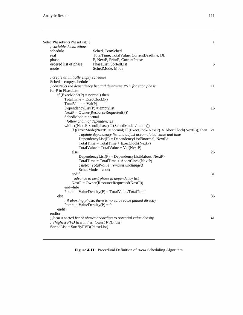
Analytic Results 111
SelectPhaseProc(PhaseList) { 1; variable declarationsschedule Sched, TentSchedreal TotalTime, TotalValue, CurrentDeadline, DLphase P, NextP, PriorP, CurrentPhaseordered list of phase PhaseList, SortedList 6mode SchedMode, Mode
; create an initially empty scheduleSched = emptyschedule; construct the dependency list and determine PVD for each phase 11for P in PhaseList
if (ExecMode(P) = normal) thenTotalTime = ExecClock(P)TotalValue = Val(P)DependencyList(P) = emptylist 16NextP = Owner(ResourceRequested(P))SchedMode = normal; follow chain of dependencieswhile ((NextP ≠ nullphase) ∧ (SchedMode ≠ abort))
if ((ExecMode(NextP) = normal) ∧ (ExecClock(NextP) ≤ AbortClock(NextP))) then 21; update dependency list and adjust accumulated value and timeDependencyList(P) = DependencyList⋅<normal, NextP>TotalTime = TotalTime + ExecClock(NextP)TotalValue = TotalValue + Val(NextP)
else 26DependencyList(P) = DependencyList⋅<abort, NextP>TotalTime = TotalTime + AbortClock(NextP); note: ‘TotalValue’ remains unchangedSchedMode = abort
endif 31; advance to next phase in dependency listNextP = Owner(ResourceRequested(NextP))
endwhilePotentialValueDensity(P) = TotalValue/TotalTime
else 36; if aborting phase, there is no value to be gained directlyPotentialValueDensity(P) = 0
endifendfor; form a sorted list of phases according to potential value density 41; (highest PVD first in list; lowest PVD last)SortedList = SortByPVD(PhaseList)
Figure 4-11: Procedural Definition of DASA Scheduling Algorithm
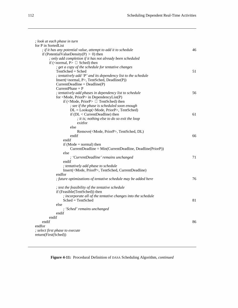
112 Scheduling Dependent Real-Time Activities
; look at each phase in turnfor P in SortedList
; if it has any potential value, attempt to add it to schedule 46if (PotentialValueDensity(P) > 0) then
; only add completion if it has not already been scheduledif (<normal, P> ∉ Sched) then
; get a copy of the schedule for tentative changesTentSched = Sched 51; tentatively add ‘P’ and its dependency list to the scheduleInsert(<normal, P>, TentSched, Deadline(P))CurrentDeadline = Deadline(P)CurrentPhase = P; tentatively add phases in dependency list to schedule 56for <Mode, PriorP> in DependencyList(P)
if (<Mode, PriorP> ∈ TentSched) then; see if the phase is scheduled soon enoughDL = Lookup(<Mode, PriorP>, TentSched)if (DL < CurrentDeadline) then 61
; it is; nothing else to do so exit the loopexitfor
elseRemove(<Mode, PriorP>, TentSched, DL)
endif 66endifif (Mode = normal) then
CurrentDeadline = Min(CurrentDeadline, Deadline(PriorP))else
; ‘CurrentDeadline’ remains unchanged 71endif; tentatively add phase to scheduleInsert(<Mode, PriorP>, TentSched, CurrentDeadline)
endfor; future optimizations of tentative schedule may be added here 76
; test the feasibility of the tentative scheduleif (Feasible(TentSched)) then
; incorporate all of the tentative changes into the scheduleSched = TentSched 81
else; ‘Sched’ remains unchanged
endifendif
endif 86endfor; select first phase to executereturn(First(Sched))
Figure 4-11: Procedural Definition of DASA Scheduling Algorithm, continued
Analytic Results 113
3. Lookup(element, orderedlist)returns the key value associated with the first occurrence of element in listorderedlist.
4. First(orderedlist) returns the first element in list orderedlist.
5. SortByPVD(phaselist)returns a list of phases ordered by decreasing PVD; if two or more phaseshave the same PVD, then the phase or phases with the greatest requiredexecution time (ExecClock) appear before any others with the same PVD.
6. Feasible(orderedlist)returns a boolean value (true or false) indicating whether the schedulerepresented by orderedlist, an ordered list of mode-phase pairs,constitutes a feasible schedule, as defined previously (by the functionfeasible() in Section 3.2.1.3).
7. Min(x, y) returns the minimum of x and y.
Briefly, the procedure consists of four stages. First, each phase is examined to determine its potential
value density and to construct its dependency list. Second, the phases are sorted and placed into an ordered
list ranked by their PVD. Next, a schedule is constructed by attempting to add each phase, along with all of
the other phases in its dependency list, to the evolving schedule. If this addition produces a feasible
schedule, then the phase is included in the schedule; otherwise, it is not. (Some simplifications of the
evolving schedule occur at this point as well.) Finally, after all of the phases have been considered for
inclusion in the tentative schedule, the schedule’s first element is selected for immediate execution.
The schedule created by the SelectPhaseProc() procedure is an ordered list of mode-phase pairs, each
placed according to the deadline it must meet. So, for instance, a phase that must meet a deadline at time
t = 1 will precede a phase that must meet a deadline at time t = 2 in the schedule. If more than one phase
must meet a single deadline, then the mode-phase pair that was added to the schedule last will be executed
first.
Notice that the deadline a mode-phase pair must meet is not necessarily the deadline associated with that
phase. In fact, the phase may need to meet an earlier deadline in order to enable another phase to meet its
time constraint. Whenever a phase is considered for insertion in the tentative schedule (line 47 of Figure
4-11), it is scheduled to meet its own time constraint. However, all of the mode-phase pairs in its
dependency list must execute before it can execute, and, therefore, must precede it in the schedule.
The variable CurrentDeadline is used in SelectPhaseProc() to keep track of this type of scheduling
consideration. Initially, it is set to be the deadline of the phase to be tentatively added to the schedule.
Thereafter, any mode-phase pair that has a later time constraint than CurrentDeadline is required to meet
CurrentDeadline. If, however, a mode-phase pair has a tighter deadline than CurrentDeadline, then it is
scheduled to meet the tighter deadline, and CurrentDeadline is advanced to that time since all of the
mode-phase pairs left in the dependency list must complete by then.
The major data structures used by SelectPhaseProc() are:1. a Phase Control Block (PCB) for each phase to be scheduled −− it contains a phase id, the
necessary scheduling parameters (ExecMode, ExecClock, AbortClock, Deadline, Value, the
114 Scheduling Dependent Real-Time Activities
names of any currently requested or held shared resources, a reference to a dependency list,and a reference to another phase that is used to chain PCBs together to form the PhaseList;
2. PhaseList is simply a reference to the first phase in the list; subsequent phases in the list arefound by following the phase reference field in the PCBs;
3. SortedList is simply an ordered list of references to the PCBs;
4. dependency lists are linked lists of mode-phase pairs, each of which refers to a specific PCB;
5. schedules are ordered lists of mode-phase pairs; although many data structures may be45sufficient, assume a balanced binary tree is used here (for example, a 2-3 tree as defined in
[AHU 74]); then insert, remove, lookup and find minimum operations can all be done inO(log N) time and O(N) space for a set of N phases.
4.3.3.2. Proof: Procedural Version of DASA Is Polynomial in Space and Time
Given the definition of SelectPhaseProc(), it is possible to demonstrate that the space and time that are
required to select a phase for execution are bounded by the problem size −− that is, the number of phases
requesting to be scheduled −− raised to a constant power.
Theorem 4: Given N phases to be scheduled using the DASA scheduling algorithm, SelectPhaseProc()2will determine the first phase to execute in O(N log N) time.
Proof. To determine the time required by SelectPhaseProc(), examine the amount of time required for
each of its component steps:1. Create an initially empty schedule (lines 9-10): O(1), this requires constant time for virtually
any list structure.
22. Construct the dependency list and determine PVD for each phase (lines 11-40): O(N ), since:a. the for loop beginning at line 12 is executed N times, once for each phase;
b. if the ExecMode of the phase is not normal, then the loop body takes O(1) time toexecute (it is a single assignment statement, lines 37-38); however, if the ExecMode isnormal, then loop body takes O(N) to execute since:
i. lines 14-18 require O(1) time;
ii. because there are no deadlocks, there can be no circular dependency lists;therefore, the while loop at line 20 will be executed less than N times, and eachtime lines 21-33 require O(1) time; hence the entire while loop requires O(N)time to execute in the worst case;
iii. line 35 requires O(1) time;
3. Form a sorted list of phases according to potential value density (lines 41-43): O(NlogN) ifany of a number of standard sorting algorithms are used (for example, heap sort as defined in[AHU 74] or any other standard text on algorithms);
24. Tentatively add each phase in turn to the schedule (lines 44-87): O(N log N), since:a. the body of the for loop at line 45 will be executed N times, once for each phase;
b. the loop body takes O(1) time to execute if the phase’s PVD is less than or equal tozero or if the completion of the phase has already been scheduled; otherwise, itrequires O(N log N) because:
45Given a specific type of application, experience may indicate that there are better data structures for schedules. For example, ifthere are typically only a few phases ready to execute, then a simple linear, linked list may be sufficient. The tree structure wasselected for generality and because it will accommodate large numbers of phases and dependencies gracefully.
Analytic Results 115
i. copying the schedule (lines 50-51) can be done in O(N) time in astraightforward manner;
ii. inserting the completion of the phase into the schedule (lines 52-53) can bedone in O(log N) time since there are at most 2N mode-phase pairs in theschedule (corresponding to an abort and a normal completion for each of the Nphases);
iii. setting up some variables for bookkeeping (lines 54-55) requires O(1) time;
iv. the for loop (lines 56-75) requires O(N log N) time since the loop will beexecuted fewer than N times and each execution will require O(log N) time toperform insert, remove, and lookup operations on the tentative schedule;
v. testing the feasibility of the tentative schedule (lines 78-79) requires O(N logN) time since it can be done by looking up each of the scheduled mode-phasepairs in order, summing execution requirements, and comparing thoserequirements to the actual available time; this requires N lookups, eachrequiring O(log N) time;
vi. incorporating all of the tentative changes into the schedule (lines 80-81)require O(N) time; this can be done by copying the N nodes that comprise thetentative schedule over the existing schedule entries;
5. Select first phase to execute (lines 88-89): O(log N) time
2Therefore, the overall time to execute SelectPhaseProc() is O(N log N).
EndOfProof
The preceding proof uses straightforward data structures and algorithms. An actual implementation may
be able to improve on these. For instance, a number of the calculations performed to compute the PVD for
each phase could be avoided if it was noted that many phases and their dependency lists do not change
between executions of SelectPhaseProc(). This optimization trades storage for speed. Similar
optimizations may bring additional savings.
Theorem 5: Given N phases to be scheduled using the DASA scheduling algorithm, SelectPhaseProc()2will determine the first phase to execute using O(N ) space.
Proof. The space required for SelectPhaseProc() consists of:1. a PCB for each phase to be scheduled −− this requires O(N) space;
2. two schedules, Sched and TentSched, each of which is a balanced binary tree with at most 2Nnodes −− this requires O(N) space;
3. space for SortByPVD() to sort the phases (actually, it will sort a set of keys that refer toindividual PCBs) −− this requires O(N) space;
4. space for each phase’s DependencyList −− this requires O(N) space for each phase in the2 46worst case, thereby requiring O(N ) space overall in the worst case ;
5. various scratch variables −− this requires O(1) space.
46This would truly be unusual. In order to have very long dependency lists for each phase, the system would have to be nearlydeadlocked and every phase would have to be close enough to completing its normal execution that it would take longer to abort thanto let it complete normally.
116 Scheduling Dependent Real-Time Activities
Putting these requirements together, it is seen that, in the worst case, SelectPhaseProc() may require2O(N ) space.
Notice that there is no mention of the storage required to track the ownership and state of each of the
shared resources in the system. This is ignored because it is information that is always maintained by the
system for any resource management or scheduling algorithm. No additional cost is imposed by the DASA
algorithm.
EndOfProof
4.4. Notes on Algorithm
The proofs presented in this chapter have allowed the behavior of the DASA scheduling algorithm to be
witnessed under specific circumstances, providing more understanding of the algorithm. This, coupled
with the algorithm’s formal definition, may suggest situations where DASA may exhibit unusual or
unexpected behavior.
Each of the following sections discusses one such situation and the attendant algorithm behavior. Where
appropriate, methods for handling the situation are also mentioned.
4.4.1. Unbounded Value Density Growth
While value density and potential value density are appealing because they allow the application to make
the best use of the processor time consumed by each phase, they also display an interesting behavior when
the required computation time to complete a phase approaches zero: the value density, which is value
divided by required computation time, becomes unboundedly large.
This can have some unexpected effects, since −− given a sufficiently short required computation time −−DASA will favor executing a phase with a very low actual value over a phase with an extremely high actual
value that requires more time. In fact, this is arguably the proper decision to make, given that the
scheduler’s objective is to maximize total value to the application, not to execute the phase with the
greatest value.
When assigning values to phases, an application designer may wish to ensure that, under any
circumstances, a given phase will be selected for execution over another phase. In order to do this, the
designer must make certain that the value density of the desired phase is always the greater of the two value
densities. However, if the value density can grow unboundedly large, then, in general, there is no way to
guarantee that the value density of one phase will always be greater than that of another phase.
Fortunately, a few facts mitigate this problem. For one thing, the required computation time for a phase
will never reach zero because if it did the phase would be done and would not be involved in scheduling
decisions. Therefore, there is a limit on how small the required computation time can be. Hence there is
Analytic Results 117
also a bound on how large a value density can grow. The application designer can use this bound to assign
values appropriately.
If that bound is deemed to be too large, then a smaller bound can be imposed by specifying a minimum
amount of computation time that may be requested for completing a phase. If a required computation time
parameter should ever be smaller than this minimum, then the minimum value should be used in its place
when applying the DASA scheduling algorithm.
Evaluating the value density associated with a phase only once, at the time of the phase’s initiation,
would also have the effect of avoiding the practically unbounded growth of value densities. The basic
information encoded into the value density metric would remain the same and would be captured
effectively. However, the benefit that arises from evaluating the value density for each scheduling decision
would be lost −− that is, there would no longer be a rising value density to indicate that for a relatively
small investment of processor cycles, a large return in application value could be realized.
4.4.2. Idle Intervals During Overload
DASA is not optimal. It is a heuristic that does well according to important metrics for the class of
real-time supervisory control applications. However, there are overload situations where it can be less
effective than other scheduling algorithms.
DASA constructs a schedule by successively adding activities that have the highest PVDs. In this way,
each time an activity, along with any other activities on which it depends, is added to the tentative schedule,
DASA is getting the greatest amount of value for the processing cycles that are then reserved for those
activities. (If any other activity could yield more value for those processor cycles, it would −− by
definition −− have a higher PVD. But all of the activities with a higher PVD that can be feasibly scheduled
have already been added to the tentative schedule.)
LBESA adds activities to a schedule according to the nearness of their deadlines; and, in case of an
overload, it sheds the activities with the lowest PVDs until a feasible activity is obtained. As shown in
Section 4.3.2.4, LBESA may shed some activities that can be included in a schedule. This can result in
LBESA utilizing fewer processor cycles than DASA in a given situation.
The factors discussed in the previous paragraphs can collectively yield a situation where LBESA can
produce a schedule representing a higher value to an application than can DASA. For instance, consider an
application consisting of three activities, each of which has only a single phase. The phases are designated
p , p , and p , respectively. Furthermore, assume that at time t = 0 the following conditions hold (using the1 2 3
notation for the scheduling automata):
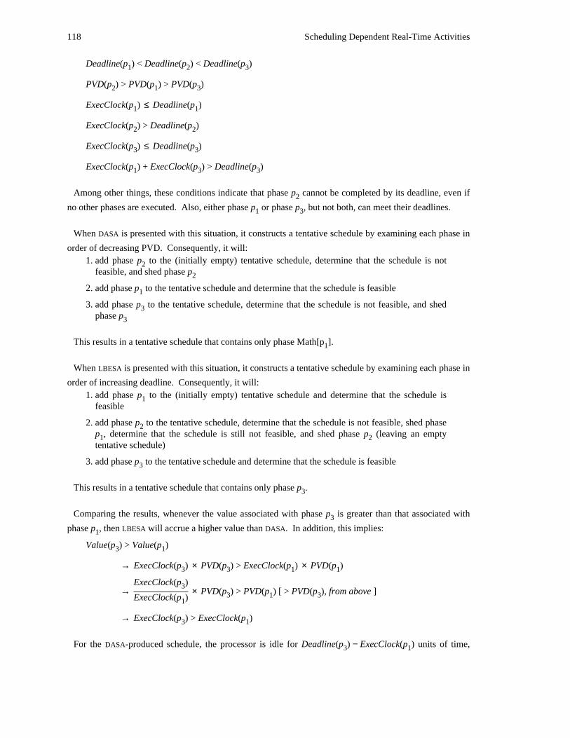
118 Scheduling Dependent Real-Time Activities
Deadline(p ) < Deadline(p ) < Deadline(p )1 2 3
PVD(p ) > PVD(p ) > PVD(p )2 1 3
ExecClock(p ) ≤ Deadline(p )1 1
ExecClock(p ) > Deadline(p )2 2
ExecClock(p ) ≤ Deadline(p )3 3
ExecClock(p ) + ExecClock(p ) > Deadline(p )1 3 3
Among other things, these conditions indicate that phase p cannot be completed by its deadline, even if2
no other phases are executed. Also, either phase p or phase p , but not both, can meet their deadlines.1 3
When DASA is presented with this situation, it constructs a tentative schedule by examining each phase in
order of decreasing PVD. Consequently, it will:1. add phase p to the (initially empty) tentative schedule, determine that the schedule is not2
feasible, and shed phase p2
2. add phase p to the tentative schedule and determine that the schedule is feasible1
3. add phase p to the tentative schedule, determine that the schedule is not feasible, and shed3phase p3
This results in a tentative schedule that contains only phase Math[p ].1
When LBESA is presented with this situation, it constructs a tentative schedule by examining each phase in
order of increasing deadline. Consequently, it will:1. add phase p to the (initially empty) tentative schedule and determine that the schedule is1
feasible
2. add phase p to the tentative schedule, determine that the schedule is not feasible, shed phase2p , determine that the schedule is still not feasible, and shed phase p (leaving an empty1 2tentative schedule)
3. add phase p to the tentative schedule and determine that the schedule is feasible3
This results in a tentative schedule that contains only phase p .3
Comparing the results, whenever the value associated with phase p is greater than that associated with3
phase p , then LBESA will accrue a higher value than DASA. In addition, this implies:1
Value(p ) > Value(p )3 1
→ ExecClock(p ) × PVD(p ) > ExecClock(p ) × PVD(p )3 3 1 1
ExecClock(p )3→ × PVD(p ) > PVD(p ) [ > PVD(p ), from above ]3 1 3ExecClock(p )1
→ ExecClock(p ) > ExecClock(p )3 1
For the DASA-produced schedule, the processor is idle for Deadline(p ) − ExecClock(p ) units of time,3 1
Analytic Results 119
while for the LBESA-produced schedule, the processor is idle for Deadline(p ) − ExecClock(p ) units of3 3
time. Therefore, the schedule produced by DASA has more idle time than the one produced by LBESA −−even though there is an overload and two of three phases that were known to the scheduler were shed.
Consequently, by executing an activity with a lower value density for a long enough time, while the DASA
scheduler is forced to leave the processor idling, LBESA can accrue a greater value than DASA for an
application.
DASA could be altered to detect relatively long idle periods during overload. Then, whenever such a
period was found, DASA could employ a special-purpose scheduling strategy. For instance, it could add
phases to the tentative schedule in decreasing order of value, rather than decreasing order of potential value
density. In the future, variations in the algorithm along those lines may be explored, as indicated in the
brief discussion in Section 7.4.3.
The simulation results in the next chapter demonstrate the effects of idle intervals during overloads and
show that these intervals occur infrequently for the simulated workloads. In particular, Section 5.2.3.2
explicitly addresses this topic.
4.4.3. Cleverness and System Dynamics
The applications of interest for this research are by nature dynamic. A scheduler must be able to react
dynamically in order to produce effective schedules for these applications.
Yet there is a balance to be struck. The more information that is used to make scheduling decisions, the
better-informed the decisions are. This typically results in better scheduling decisions. On the other hand,
each decision is made based on the best information available at the time of the decision. At any point
thereafter, circumstances may change −− a new request may be made for a shared resource or new activities
may arrive to be scheduled −− demanding that new scheduling decisions be made, possibly resulting in
undoing some previously accomplished work.
Intuitively, the more dynamic and unpredictable an application is, the less appropriate clever (read
"time-consuming") scheduling schemes are. The actual dividing line for this decision is not clear in
general. The simulations in the following chapter demonstrate DASA’s performance in various situations
and take into account the amount of time required to make scheduling decisions. In fact, the simulator
could be used to determine the effectiveness of the DASA scheduling algorithm compared to another
algorithm for any application.

120 Scheduling Dependent Real-Time Activities
Chapter 5
Simulation Results
The previous chapter employed formal analysis techniques to demonstrate that the DASA algorithm
possesses desirable properties. However, the formal analysis could not compare DASA to every other
algorithm of interest in arbitrary situations. Nor could it quantify the gains that could be realized by using
DASA to schedule specific workloads. Simulations were performed to examine these issues, and the
simulation results are described in this chapter.
Section 5.1 discusses the design and implementation of the simulator used to evaluate DASA and other
scheduling algorithms.
Sections 5.2, 5.3, and 5.4 present results generated with the simulator to evaluate the performance of the
DASA scheduling algorithm. These results demonstrate that dependency, importance, and urgency data are
used by DASA to schedule a processor more effectively than any of the other algorithms tested when there
are shared resources and high processor loads. In fact, DASA degrades gracefully as processor load
increases, becoming more effective relative to the other algorithms at higher load levels. The simulations
account for the amount of time that is spent making scheduling decisions for each algorithm, and identify
the point at which the time spent executing the DASA algorithm becomes counterproductive. Further
simulations show that DASA can meet more deadlines and accrue more value on behalf of the application by
issuing aborts in order to free previously allocated resources in certain situations, but this effect is fairly
small.
Finally, Section 5.5 hypothetically characterizes two real-time applications, identifying their salient real-
time characteristics and outlining how simulation results similar to those presented here could be applied to
determine the effectiveness of using DASA to schedule these applications.
5.1. Simulator Design and Implementation
The first part of this section outlines the set of requirements that the simulator had to meet. The rest of
the section describes the design that was adopted and discusses significant implementation issues.
121
122 Scheduling Dependent Real-Time Activities
5.1.1. Requirements
Fundamentally, the simulator must allow DASA to schedule a variety of workloads. In fact, there are a
number of ways in which this may be accomplished. Therefore, to guide the simulator development, the
following general requirements were adopted:1. support a variety of workloads conforming to the computational model presented earlier −−
that is, the simulated workload represents a real-time supervisory control application, whichis composed of a number of activities, each of which may have one or more computationalphases. The activities may share resources as outlined previously in this work. And all of theassumptions concerning the information that is available to the scheduler, such as the amountof computation time to complete each phase, continue to hold. The set of applications thatcan be run must be rich in order to allow a significant range of applications to be explored.
2. offer standard statistical distributions for use by the application −− to examine the behavior ofa scheduler under general conditions, it is often convenient to assume that events occurtemporally according to a standard statistical distribution, such as a normal or a Poissondistribution.
3. incorporate useful metrics and gather statistics −− the metrics are intended to aid in theevaluation of scheduler performance. For instance, the number of time constraints satisfied,the number not satisfied, and the total application-specific value accrued are allstraightforward examples of useful metrics that the simulator should support.
4. allow evaluation of multiple scheduling algorithms and resource management policies −− theprimary objective of the simulations is to compare the performance of DASA with that of otheralgorithms. Therefore, the simulator must accommodate a set of well-known schedulingalgorithms, including priority, deadline, and best-effort schedulers. In addition, since DASAalso makes all of the shared resource management decisions, the simulator must provideseveral alternative resource management policies, including FIFO and deadline queueing forshared resources that are not available.
5. provide a trace of the scheduling events and decisions made during a simulation −− thisinformation is useful for at least three reasons: (1) it allows a detailed inspection of schedulerbehavior to identify specific beneficial or detrimental decisions, (2) it makes available rawdata that may be processed to generate other meaningful statistics for any specific scheduler,and (3) during the initial implementation or subsequent modification of a schedulingalgorithm, the event trace can be examined by hand or by machine to demonstrate correctbehavior.
6. possess the flexibility to adapt to changing requirements or to augment the initial capabilitiesof the simulator −− since the simulator is used to examine algorithms under a wide range ofcircumstances and the appropriate metrics are not necessarily known in advance, flexibility isdesirable. In addition, if the simulator is to be useful over time, it will have to be able toaccommodate new algorithms that will be developed, which may or may not resemble thosethat already exist. By choosing internal interfaces carefully, this is not too demanding arequirement.
The simulator developed meets all of these requirements, as explained in the following sections.
5.1.2. Design
The simulator design compartmentalized major functions so that different workloads and scheduling
algorithms could be accommodated. As shown in Figure 5-1, the simulator features several independent
parts:1. a set of shared resources,
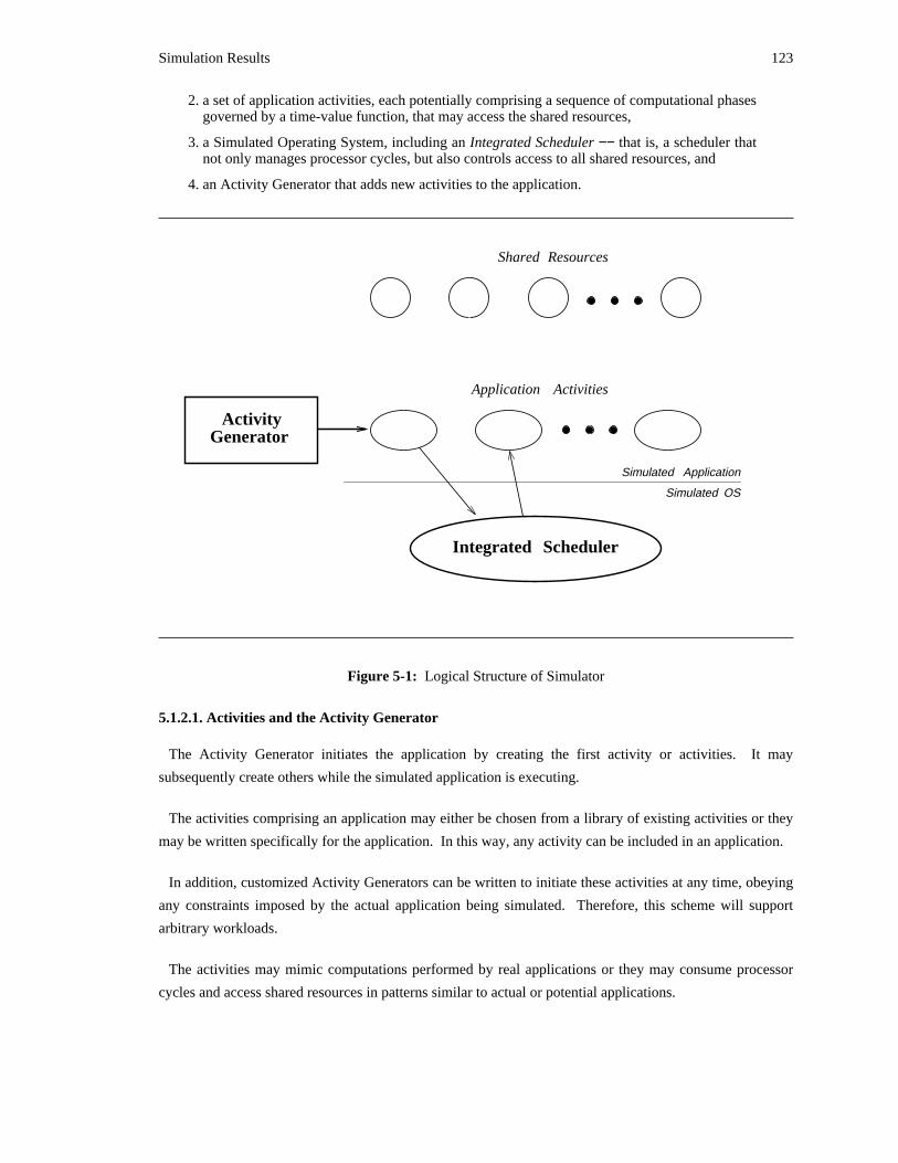
Simulation Results 123
2. a set of application activities, each potentially comprising a sequence of computational phasesgoverned by a time-value function, that may access the shared resources,
3. a Simulated Operating System, including an Integrated Scheduler −− that is, a scheduler thatnot only manages processor cycles, but also controls access to all shared resources, and
4. an Activity Generator that adds new activities to the application.
Integrated Scheduler
Simulated OS
Simulated Application
Application Activities
Shared Resources
ActivityGenerator
Figure 5-1: Logical Structure of Simulator
5.1.2.1. Activities and the Activity Generator
The Activity Generator initiates the application by creating the first activity or activities. It may
subsequently create others while the simulated application is executing.
The activities comprising an application may either be chosen from a library of existing activities or they
may be written specifically for the application. In this way, any activity can be included in an application.
In addition, customized Activity Generators can be written to initiate these activities at any time, obeying
any constraints imposed by the actual application being simulated. Therefore, this scheme will support
arbitrary workloads.
The activities may mimic computations performed by real applications or they may consume processor
cycles and access shared resources in patterns similar to actual or potential applications.
124 Scheduling Dependent Real-Time Activities
Whenever necessary, an activity will interact with the Simulated Operating System to acquire specific
services. The requests made to the Integrated Scheduler, such as requesting the start of a new
computational phase or requesting access to a shared resource, are of particular interest for this research.
5.1.2.2. Integrated Scheduler
The interface to the Integrated Scheduler conforms to the interface described in Section 2.3.2 for the
General Scheduling Automaton Framework, incorporating scheduling events that are concerned with both
processor cycle management and shared resource management.
Scheduling algorithms are embodied in Integrated Schedulers, and different scheduling algorithms can be
compared by executing the same application using various Integrated Schedulers.
The requests made of the Integrated Scheduler can naturally be divided into two groups: (1) those that
deal fundamentally with phase execution (that is, ‘request-phase,’ ‘abort-phase,’ ‘preempt-phase,’ and
‘resume-phase’) and (2) those that deal fundamentally with resource management (that is, ‘request’ and
‘grant’). Traditionally, these two groups of requests have been handled by two different entities −− the
scheduler and the resource manager, respectively. The simulator design at the highest (interface) level
hides that distinction. Internally, however, for typical scheduling algorithms requests are routed to the
scheduler or the resource manager.
On the other hand, DASA is an integrated scheduling algorithm in this sense, and so all of the requests
originating from application activities are directed to the DASA scheduling module.
5.1.3. Implementation
Given a design, the implementation of the simulator raises several new issues, including the selection of
the tools to build the simulator, the languages to be used, the interface presented to the experimenter, and
the structure of the implementation. Some of the more interesting aspects of these issues are discussed in
the following paragraphs.
5.1.3.1. Approach: Build from Scratch or Adapt an Existing Simulator
There are several different approaches that may be used to produce the simulator described above, and
selecting one of them is the first major implementation issue to be resolved. For example, the simulator
may be custom-built from scratch. This approach allows the simulator to be precisely tailored to meet the
goals of this investigation. On the other hand, if an existing simulator could be found that is similar in
purpose to the desired simulator, then it might be modified to satisfy the present goals. Possibly, this could
be done quickly to generate useful results.
In fact, the approach used −− writing the simulator using SIMSCRIPT II.5, a programming language
intended for simulations −− falls between those two extremes. It builds on previous work, while allowing a
large degree of customization.
Simulation Results 125
SIMSCRIPT provides a basic framework and a number of useful libraries, including a random number
generator and a full complement of probability distributions. Using SIMSCRIPT obviates the need to
reimplement and debug these features for a simulator. In addition, SIMSCRIPT provides a programming
abstraction called a process that is well-suited to model an activity. These processes may control their own
(virtual) execution, as well as that of other SIMSCRIPT processes. The code that comprises the Integrated
Scheduler is executed by processes when they initiate a scheduling event. The scheduling algorithm
dictates the resulting outcome: either the executing process will continue to run or it will block itself while
unblocking its successor. Programming constructs exist to consume (virtual) execution time, and
SIMSCRIPT manages the advancement of virtual time.
SIMSCRIPT also supports a programming abstraction called a resource to embody shared resources.
However, this abstraction, although providing the services of a typical resource manager, was not flexible
for the purposes of this work, where the resource management decisions are more closely tied to scheduling
decisions. Therefore, some of the resource features of SIMSCRIPT were superceded for these simulations.
The use of a simulation programming language provided sufficient freedom so that the Integrated
Scheduler could be implemented in the modular fashion described in the design discussion. If an existing
simulator had been chosen as the vehicle for this work rather than a simulation language, then the
organizational structure imposed by the simulator might have precluded this possibility.
5.1.3.2. Source of DASA Implementation
The version of the DASA scheduling algorithm that was included in the simulator was adapted from the
procedural version of the algorithm presented in Section 4.3.3.1. A procedural version had to be used since
SIMSCRIPT is a procedural language. A straightforward translation converted the Section 4.3.3.1 version
into a SIMSCRIPT version.
There were two differences in the simulator version of DASA, compared to the procedural version
presented earlier. Specifically:1. Feasibility testing is slightly different. In the procedural version in Section 4.3.3.1, a
schedule is only feasible if all phases that execute normally (as opposed to aborting) meettheir deadlines. This may be an unnecessarily strict definition of feasibility. For instance, ifthe only reason a given phase is executed is to allow it to release a shared resource that isneeded for a second phase, and it is quicker to complete the phase normally that it is to abortit, then scheduling its normal completion is perfectly reasonable under the model that has
47been presented in this thesis. This is true even if the phase can no longer meet its deadline .
In the simulator code, each time a phase p and the members of its dependency list are addedto the tentative schedule, phase p’s deadline must be met or the tentative additions will beremoved from the schedule. However, the phases in the dependency list do not necessarilyhave to meet their deadlines. They are tentatively placed in the schedule so that if they canfeasibly meet their deadlines, they will. But even if they cannot meet their deadlines they willremain in the schedule if phase p does.
47As stated, this makes sense under the model presented here. In some real-time systems, completing a phase late could result insome problems, implying that executing such a phase normally is a mistake if it cannot complete on time. In other real-time systems,it is not possible to abort an arbitrary phase at any time, implying that aborts cannot always be performed to release an allocatedresource. There is no clear action that will work for all systems. Experience gathered using time-driven scheduling techniques willhelp resolve this question in the future.
126 Scheduling Dependent Real-Time Activities
All subsequent feasibility tests continue to test the feasibility of each of the deadlines thathave been designated as critical, as explained in the previous paragraph.
2. As defined in Section 4.3.3.1, if DASA determines that there is no phase that can feasibly meetits deadline, it will allow the processor to idle, rather than run a phase that cannot satisfy itstime constraint. This is unusual behavior for a scheduler, but it makes sense under the modelpresented.
There is one situation in which executing a phase would be more desirable than idling, eventhough no phase can meet its deadline: if one of the infeasible phases is holding one or moreshared resources. The processor cycles that would otherwise be spent idling could instead beused to free these resources. This can save time in the future since the processor cycles willhave to be spent to free the resources once a request has been made by a phase that can satisfyits time constraint.
Based on this rationale, the simulator’s version of DASA will select a phase that is holdingshared resources and execute it (in either ‘normal’ or ‘abort’ mode, whichever requires fewerprocessor cycles) if there is nothing to feasibly execute.
5.1.3.3. Single Scheduler for Simulation
The simulator uses only a single scheduling algorithm (and associated resource queueing discipline) for a
given simulation run. The simulator allows the arrival of new activities and phases to be regenerated
exactly for specified simulation runs. Therefore, comparing two scheduling algorithms requires two
different simulation runs, one for each of the algorithms. Both runs present identical input to the
scheduling algorithms. A subsequent examination of the statistical metrics and the scheduler performance
for each run can then reveal which algorithm was more effective in the simulated situation.
5.1.3.4. Simulator Display Messages
By default, the simulator displays all of the key information regarding a simulation run to the
experimenter. This includes a timestamped message announcing the arrival of each new computational
phase that must be scheduled, along with its time constraint, required execution time, value, the number
and identity of the shared resources that it will require, and the time interval between each pair of shared
resource acquisitions (in terms of actual execution time, not real time). Notice that although the simulator
prints information about shared resource needs of a phase at its outset, this information is not available to
the scheduling algorithms when the phase is initially presented to the scheduler. Rather, each new resource
request is made by the phase at the moment the resource is needed. Only at that point is the scheduler
made aware of the need for that particular resource. The information about all of a phase’s resource
requirements is printed out when the phase initially arrives only as a minor user convenience −− it allows
all of the requirements information for the phase to be presented together in one place.
Other time-stamped messages are displayed to the experimenter each time a resource is requested or
granted or a phase is preempted, resumed, or aborted.
Additionally, a simulation profile is printed that identifies the scheduling algorithm and resource
queueing discipline employed, the number of shared resources available, and other workload specific
statistics, such as the average interarrival time between phases or the average required execution time for
each type of phase.
Simulation Results 127
Finally, a statistical summary of the simulation is displayed at the conclusion of the run. It prints general
statistics including the total number of phases, the number that met their time constraints, the total value48represented by all of the phases , and the value actually accrued by the scheduler during the simulation.
49Other statistics that are of interest for a specific scheduler or workload can also be displayed at the
conclusion of the simulation.
All of the messages displayed to the experimenter can be redirected to a file to record the simulation
results for later analysis. In this case, the experimenter is offered a summary of the simulation in addition
to the log file.
5.1.3.5. Modifications
There are a number of modifications that may be made to the existing simulator, and these modifications
can be divided into two groups. First, there are the changes that the simulator was designed to
accommodate, for instance, the addition of a new scheduling algorithm or a new resource queueing
discipline. Second, there are changes that may be anticipated, but were not specifically provided for in the
simulator. Extending the simulator to handle multiprocessor scheduling is an example of the latter type of
change.
Provisions have been made to facilitate the anticipated modifications of adding new scheduling and
resource queueing policies. To add a new policy, a set of routines must be written, one routine to handle
each scheduling event. These routines are named according to an existing convention. The name of the
policy is added to the menu of policies available to the experimenter. And finally, the new routines are
compiled and linked with the existing simulator.
Since the information required or the data structures used by different scheduling policies may vary
significantly, new data fields and structures may be associated with each activity or computational phase.
Once again, a naming convention has been adopted for labeling these fields and structures to avoid
conflicts with existing fields and structures.
The simulator has been structured carefully so that modifications that could not be anticipated precisely
can be handled gracefully. There is no single point in the simulator where all statistics may be gathered
and processed. As new statistics are defined, it is likely that at least some of them will have to be inserted
in code at locations determined strictly by the scheduling algorithm being examined.
Preparations have been made for some other potential modifications. Some data structures have been
defined to be more general than necessary for the purpose at hand. For instance, the number of application
48Notice that it may not be possible to attain this value, even with complete knowledge of the phases and their requirements.Attaining this total value may be impossible due to insufficient processing cycles or resource availability for some portion of thesimulation. It does serve as a clear upper bound on the value that may be obtained by any scheduler.
49Average lateness, indicating the amount by which phases miss deadlines, is only of interest for some schedulers. In particular, itis not informative for either DASA or LBESA since they both shed excess load and do not generally bother to complete any phase thatcannot meet its deadline. For them, once an overload occurs, the average lateness becomes infinite.
128 Scheduling Dependent Real-Time Activities
processors that are being scheduled is a variable and there is an array containing the relevant state for each
of the currently executing activities. Of course there is only one executing activity under the model being
investigated by this work. However, in the future the simulator framework may be able to accommodate
multiprocessor scheduling. At that time, many, if not all, of the scheduling algorithms will have to be
modified to handle multiprocessor scheduling and to use the simulator’s data structures in a more general
way. This will probably require a significant amount of work, but the existing simulator framework should
prove useful in minimizing the overall effort.
5.2. Evaluation of DASA Decisions
This section evaluates the decisions that DASA makes compared to the decisions made by other
scheduling algorithms and resource queueing disciplines.
The experiments described in this section assume that scheduling decisions are made instantly. This
affords an opportunity to measure the improvement in decision quality that results from using additional
information when making scheduling decisions. (Sections 5.3 and 5.4 both report experimental results that
take into account the amount of time required to make scheduling decisions. They indicate behavior that
could be witnessed in actual implementations.)
A general, parameterized workload is used to exercise the simulator with varying degrees of processor
utilization and varying numbers of shared resources.
5.2.1. Methods of Evaluation
The utility of a scheduling algorithm may be demonstrated in a number of different ways. The following
paragraphs deal with four major approaches that correspond to four different workload sources.
5.2.1.1. Execute Existing Applications
Perhaps the most compelling method would be to employ the algorithm in an instrumented, production
system and compare the system performance directly to its performance using other algorithms. Using this
approach would yield the most direct, relevant information regarding the applicability of the scheduler for a
given application.
There are three major problems with this direct approach. First, although it definitely evaluates the
performance of the scheduler for a specific application, it is not clear that the information gathered can be
applied to any other applications, and if can, under what circumstances. Since this work is addressing a
general problem, the ability to make statements that apply to a general class of applications is desirable.
If a wide range of existing applications can be executed directly, this problem can be eliminated and more
general results can be derived. However, since many real-time systems today are still custom-designed
with customized or proprietary operating systems, finding a large number of real applications that execute
Simulation Results 129
under the same operating system may be difficult. Alternatively, modifying the schedulers of several
different operating systems may be very difficult logistically.
The second major problem with the direct approach is more specific to the DASA algorithm: the
algorithm is significantly different than those that are used in practice today, and it expects that the
application will provide the scheduler with more information than is normally the case. (Specifically, the
scheduler should be given an estimate of the required computation time needed to execute each new
computational phase.) Although this information is often known to application designers and
implementers, it is not communicated to the scheduler. As a result, the interface to the scheduler that the
application sees is different for the DASA algorithm than for traditional algorithms. This requires that
every application used must be altered to provide that additional information to the scheduler, possibly long
after the people who knew the information are no longer available or able to provide it.
The final major problem results from the fundamental difference in philosophy between traditional
real-time systems and the more dynamic systems that could employ a scheduling algorithm such as DASA.
Traditionally, many real-time systems are designed to be quite specialized with minimal overhead resulting
from operating system functions. In fact, the designers of these systems attempt to eliminate operating
system functions insofar as possible, often either reducing the operating system to the point where it is
more correctly termed an executive (see the discussion in Section 1.2) or eliminating it entirely by having
the application perform all required functions.
In such real-time systems, not only are operating system functions limited, but the information supplied to
the operating system is minimal. For example, the computational and timing requirements of a given set of
activities may be sufficiently studied so that it is possible to replace a priority scheduler, for example, with
a list scheduler or a rate-group scheduler. Neither the list scheduler nor the rate-group scheduler display
dynamic behavior −− at predetermined times they dispatch predetermined activities. All timing and
dependency considerations have already been taken into account by the system designers, and the real-time50system is unaware of any of this information .
As a result, the implementations of real-time systems traditionally distort the application’s structure. For
example, often physical processes are modeled as periodic, even if they are not, in order to simplify
scheduling and increase system predictability. Or shared data is accessed directly (without using an access
control mechanism such as a lock) because the activities have been designed and placed in a sufficiently
static schedule that it can be demonstrated that no conflicts can occur.
The philosophy underlying DASA resides at the opposite end of the spectrum: in order to handle dynamic
applications today and to effectively accommodate application modifications tomorrow, the system always
decides which activities should be run, relying on key information supplied by the application. Rather than
50One of the most unfortunate aspects of such systems becomes evident when they must be modified −− perhaps to implement anew function or to add an improved device. Then all of the timing and dependency analyses must be performed again. In fact,modifying such systems may cost as much as, or more than, the original implementation. [Hatley 86] points out that not only dochanges cost a great deal, but they may also affect (logically) unrelated parts of the system.
130 Scheduling Dependent Real-Time Activities
changing the application in order to restrict the information passed to the operating system in the hope of
reducing the run-time computation performed by the system −− rendering the application difficult to adapt
along the way −− the application is encouraged to provide the system with as much relevant information as
possible, thereby potentially allowing the system to make better decisions on behalf of the application.
Unfortunately, this philosophical difference implies that the same application designed and implemented
according each philosophy will produce very different code. Once again, this limits the ability to validate
the effectiveness of DASA by simply using it to schedule existing applications. It is quite possible, for
example, that an existing application employs shared memory but, as mentioned above, never issues any
requests for access to the shared resource because an appropriately restrictive schedule makes it
unnecessary. It is extremely unlikely that DASA could demonstrate improved performance under such
constraints.
5.2.1.2. Modifying or Reimplementing Existing Applications
The preceding discussion emphasizes the difficulties involved in using existing applications directly to
evaluate DASA.
Two of the problems mentioned above −− DASA requiring more information than is traditionally supplied
to a scheduler and implementations that hide application structure and information from the operating
system −− can be addressed by modifying existing implementations or by reimplementing them. The new,
resulting implementations could then be executed using several different schedulers to evaluate the relative
effectiveness of each scheduling algorithm. However, in order to justify any results gained by this
approach, the new implementations would have to be verified in some manner. Specifically, they would
have to be demonstrably equivalent to the original implementations in all important respects. For real
applications, which are often large and complex, this vague-sounding requirement could be arbitrarily
difficult to satisfy.
5.2.1.3. Modeling Existing Applications
Creating skeletal applications that represent real applications reduces the amount of work required to
produce each application, but complicates the problem of proving that an abstracted application
corresponds to the real application in all important ways since, by definition, some details of the application
will have been discarded. Justifying that the selection of which details should be retained and which should
be eliminated or how all or part of the application should be modeled is once again a vague requirement
that would have to addressed in an ad hoc manner for each application in all likelihood.
As with each of the preceding approaches to providing a workload to use to evaluate the DASA scheduling
algorithm, this method is only capable of providing information concerning the specific workloads used.
There is no guarantee that those applications are representative of real-time supervisory control applications
in general, and these limitations must be addressed.
Simulation Results 131
5.2.1.4. Simulating the Execution of a Parameterized Application
The final potential approach to evaluate DASA, and the one actually used, employs a parameterized
application or set of applications. The execution of these applications can then be simulated under various
scheduling algorithms and performance measured. By selecting useful parameters and varying them over
ranges of values more general results can be obtained from this workload than could be drawn from a
specific set of applications.
Furthermore, the simulator built for this evaluation can be given an arbitrary application (workload). This
allows an experimenter to model a potential application with any desired amount of detail, simulate the
application’s execution using various schedulers, and decide whether the application can benefit from the
use of the DASA scheduling algorithm.
Short of building an application model for execution on the simulator, useful information is still available
to allow people with real-time applications to decide if DASA may be of interest to them. The simulation
results that follow span a significant portion of the space of real-time supervisory control applications,
based on the variation of a few key metrics. If necessary, additional simulations could be performed in the
future to extend these results to other regions of the space or to accommodate new metrics. Given the
existence of these data, an application designer or implementer can either profile an existing application or
create a thumbnail sketch of a new application to determine where the application lies in the supervisory
control space and whether any benefit may accrue if the DASA scheduler is used.
This method −− simulating the execution of parameterized applications −− was chosen to investigate the
utility of the DASA scheduling algorithm because of its ability to evaluate the algorithm over a wide range
of situations, rather than just a few specific applications. At the same time, it is able to give generally
useful information to real-time application designers and implementers for various conditions and then
allows them to investigate their application to any desired degree of detail by means of a specific model for
their application. This model can be evaluated using the DASA scheduler, as well as a number of other
schedulers of general interest. Once again, new schedulers can be added to enrich the simulator if needed
or desired.
Thumbnail sketches of real applications that may benefit from the use of the DASA scheduler are
presented in Section 5.5.
5.2.2. Workload Selection
The workload used to gather the simulation results that follow featured one basic type of activity that was
tailored according to a number of parameters.
In this workload, each activity consisted of only a single phase. However, this should not result in a loss
of generality since it is possible to model an activity comprising multiple phases as a sequence of activities,
each of which has a single phase. Then as one single-phase activity completes, the next one begins.
132 Scheduling Dependent Real-Time Activities
5.2.2.1. Arrival Times, Required Computation Times, and Values
The arrival times of the activities could be drawn from any of a number of probability distributions, and
the key parameters that define each distribution −− such as the mean and standard deviation for a normal
distribution, the minimum and maximum for a uniform distribution, or the mean for a Poisson or an
exponential distribution −− were specified by the experimenter.
Upon its arrival, the time remaining until a phase’s deadline is also drawn from a specified probability
distribution. By design, this deadline must be in the future. Once the deadline has been selected, the
phase’s required computation time is determined by multiplying the time remaining until the deadline by a
fraction drawn from a uniform probability distribution on the interval (0, 1). Hence, the initial required
computation time can never exceed the amount of time between the phase’s arrival and its deadline.
As a result, any single activity constructed in this way and executed in a system with no other activities
would meet its time constraint. Therefore, any unsatisfied time constraints occur because of the
interactions among multiple concurrent activities.
Workload parameters governing the arrival times and required computation times of activities may
generate sequences of activities that cannot possibly satisfy all of the activities’ deadlines. This is clearly
the case if the parameters specify a condition where the system is chronically overloaded −− for instance, if
the average required computation time for an activity exceeds the average interarrival time between
activities. However, even in situations where, on average, there is a significant amount of idle time, there
may be transient overload conditions due to the probabilistic nature of the workload source.
The value that is accrued when a computational phase’s deadline is met is also drawn from a specified
probability distribution. The distribution actually used for these experiments is specified in Section 5.2.3.1.
5.2.2.2. Shared Resources
The experimenter specifies the number of shared resources for a set of simulations. It is possible to
specify that there are no shared resources.
Whenever there are shared resources, each activity probabilistically determines how many of these
resources it must acquire to successfully complete its sole computational phase. Once the number of
resources has been decided, the exact identities of the shared resources that will be needed are chosen
randomly.
During the execution of a phase, these resources are requested sequentially. Each time a resource is
acquired, a fraction of the computation time remaining in the phase passes before the next resource is
requested. This fraction is drawn from a uniform probability distribution on the interval (0,1). Any
number of resources can be requested by a phase in this fashion since time is continuous.
For each shared resource, the experimenter may specify the amount of computation time that must be
spent to return the resource to a consistent, usable state should a phase holding the resource be aborted. If
Simulation Results 133
the experimenter does not specify these undo times, they are assumed to be infinite. During execution,
each time a resource is acquired by a phase, the amount of time required to abort the phase is incremented
by the undo time associated with the newly acquired resource.
Although the resources required by a phase are selected randomly, the actual resource requests are
ordered to avoid deadlocks (since deadlocks are not a primary focus of this investigation). Each resource is
associated with a unique key, and a total ordering exists over these keys. Each phase issues its resource
requests in increasing order of resource key value. Consequently, deadlock cannot occur since it is
impossible for any phase to both (a) hold a shared resource that is needed by another phase and (b) need a
shared resource already held by the same phase.
All shared resources held by a phase are released once the phase has completed execution successfully or
been aborted (as specified by the formal scheduling model).
5.2.3. Examination of DASA Behavior
A series of experiments were performed to determine the effectiveness of the DASA scheduling algorithm
relative to several other algorithms of interest. The following section describes the workload parameters
that were used for these experiments and the metrics that were used to evaluate the experimental results.
These results are presented and analyzed in Sections 5.2.3.2 and 5.2.3.3. (Subsequent sections will
investigate the effects of scheduling overhead on these algorithms and study the use of aborts to reduce
latencies utilizing the same workload.)
5.2.3.1. Workload Parameters and Metrics
These experiments, which used the parameterized workload described in the previous section, can be
divided into two groups. These groups are distinguished by the probability distributions that described
activity arrivals and selected deadlines for phase executions.
In the first group of experiments, which are analyzed in Section 5.2.3.2, the time between successive
activity arrivals, known as the interarrival time, was drawn from a uniform distribution over a specified
interval. The deadline for each activity was also drawn from a uniform probability distribution. Because
these experiments used uniform distributions to generate these parameters for each phase, they are referred
to as the U/U Distribution experiments.
The second group of experiments, which are analyzed in Section 5.2.3.3, are characterized by
exponentially distributed activity interarrival times and exponentially distributed phase deadlines.
Consequently, these experiments are referred to as the M/M Distribution experiments.
Simulator Metrics and Information Sources. A straightforward load metric is employed for all of the
simulations presented here: load is defined to be the expected time required to complete an activity (the
required computation time) divided by the expected activity interarrival time. Whenever the load is less
than 1.0, the average activity can be executed before the next activity is expected to arrive. So while there
134 Scheduling Dependent Real-Time Activities
may be transient overloads, it should still be possible to complete most of the work that arrives. On the
other hand, whenever the load is greater than 1.0, the average activity cannot be completed before the next
activity is expected to arrive. This latter situation results in a long-term overload.
The experiments utilize processor loads from 0.125 (a fairly light load) to 2.0 (where twice as many
cycles are required as are available, on average). Of course, the peak load actually exceeds 2.0 in the latter
experiments, but the experiments are of sufficient duration that the 2.0 average captures the conditions
adequately.
The information gathered by the simulator includes a few key metrics: the number of deadlines that were51met , the total value represented by all of the activities, and the value that was actually accrued by the
application during the simulation. These are subsequently reduced to percentages indicating the fraction of
deadlines that were met and the fraction of the available value that was obtained.
In addition, the simulator generates an event log that can be consulted when analyzing interesting
scenarios and evaluating decisions made by various scheduling algorithms.
Time Units. All times that are used in the experiments are expressed in terms of Time Units (TUs).
There are two reasons for referring to times in terms of TUs, rather than seconds, milliseconds, or
microseconds. First of all, different real-time applications have time constraints that cover a wide range of
absolute times. Industrial supervisory control applications typically have time constraints that are
measured in seconds or hundreds of milliseconds. Simulators and many military applications may have
time constraints that are on the order of tens or hundreds of milliseconds. And lower-level control systems
can have even tighter time constraints. By using TUs, this work is not arbitrarily associated with a single
class of application. Rather, it seems reasonable to expect that, in the future, these scheduling algorithms
can be applied to progressively more demanding real-time applications as processor speeds increase and
improved real-time computer architectures are devised.
TUs were also used to allow the results presented here to be reevaluated as technology does change. In
particular, the overhead that is incurred by using relatively complex scheduling algorithms can be
expressed in terms that reflect the technology of the time, such as the time required to perform a
multiplication or division operation or the time required to sort a list. As technology changes, the overhead
changes as well.
This can be contrasted with the real-time application being scheduled. Often, the time constraints that
must be met are dictated by the application itself −− a real world physical process that is subject to the laws
51Phases that fail to meet their deadlines can be divided into two groups: those that finish executing late and those that never finish.Each individual scheduling algorithm determines the disposition of these phases. For instance, static priority and deadline schedulerswill eventually execute every phase they encounter. So they will finish all of these phases late. However, DASA and LBESA willgenerally not execute a phase that will miss its deadline. Instead, these phases will not be scheduled and will never finish. (In a realsystem, phases that miss deadlines should probably be aborted. This is briefly discussed again in Section 5.2.3.2, where LBESAsperformance with shared resources is analyzed.)
Simulation Results 135
of physics for example. Improved computer technology does not affect these time constraints, although it
typically affects the application by reducing the amount of processor time that is required to execute any
given piece of code. So while the time constraints for a specific physical process remain fixed, the absolute
time required to execute both the application and its scheduling algorithm are reduced as technology
progresses. This will tend to increase the domain in which complex schedulers may be used in the future.
By expressing both the time constraints and the scheduling overhead in terms of TUs, it is possible to
determine what range of time constraints is appropriate for a given scheduling algorithm. To do this, a
conversion from real time units (such as milliseconds) to TUs can be computed by noting the time required
to perform the basic operations that dominate the scheduling algorithm in question, and therefore are most
responsible for its overhead. Using this conversion factor, the application time constraints can be expressed
in terms of TUs. Then, a simulation that directly mimics the application in question, including scheduling
overhead, can be run, or a more general set of simulations that take scheduling overhead into account can
be consulted to determine the applicability of a given scheduling algorithm. (An analysis of overheads for
various scheduling algorithms is presented in Section 5.3.)
52Phase Values. The values associated with the phases varied uniformly from one to ten . A minimum
value of zero was not used since that could be interpreted as a worthless process, hence one that need not be
scheduled.
Shared Resources. A fixed number of shared resources was used for each set of simulations. The
experiments featured zero, one, five, and ten shared resources. Since DASA was the only algorithm that
could abort specific phases, the undo times for the shared resources were defined to be (essentially) infinite.
In that way, DASA would not schedule aborts, and its behavior would be more comparable to that of the
other algorithms under consideration. (A look at the behavior of DASA with and without aborts is presented
in Section 5.4.)
Shared resource management for each scheduler (except DASA) is handled quite simply: if a requested
resource is available, it is immediately allocated to the activity requesting it. Otherwise, the activity is
entered in a FIFO (first-in, first-out) queue for that particular shared resource. When a resource is freed at
the completion of a computational phase, the first activity entered in its waiting queue is removed from the
queue, given access to the shared resource, and made ready to run. The scheduler may subsequently
resume its execution. (Notice that while activities are blocked waiting for a shared resource, they are not
considered by any scheduling algorithm other than DASA.)
Scheduling Algorithms. Three other scheduling algorithms were chosen to compare with DASA: DL, a
simple deadline scheduler; SPRI, a static priority scheduler; and LBESA, Locke’s Best Effort Scheduling
Algorithm.
52Preliminary simulations using wider ranges of values chosen from a uniform distribution demonstrate scheduler behavior that isvery similar to that shown in this chapter.
136 Scheduling Dependent Real-Time Activities
These algorithms illustrate a number of points. DL and SPRI apply only urgency or only importance
information, respectively, while LBESA and DASA consider both types of information. From another point
of view, DL represents the simplest type of deadline scheduler −− it simplies dispatches activities in order
of increasing deadline. If there is an overload, rather than shedding some activities, it continues to schedule
all activities in deadline order. LBESA provides an advanced load-shedding capability in a deadline-based
scheduler. And DASA continues to extend this load-shedding by considering more activities for execution
than the other algorithms. Finally, SPRI must be included since it is the algorithm that is actually used by a
large number of supervisory control applications.
Experimental Parameters. In each experiment, the parameters for phase deadline generation remained
fixed. Then for each combination of activity interarrival time parameters, number of shared resources, and
scheduling algorithm, a series of ten simulations were performed. In each simulation, 100 activities were
generated and scheduled.
The information described earlier in this section was gathered for each experiment. The following
sections provide the analysis of this information.
5.2.3.2. Scheduler Performance Analysis: U/U Distribution
The U/U Distribution experiments feature activities that have interarrival times drawn from a uniform
probability distribution. In fact, for this series of experiments, the activity interarrival time always lies
between zero and a designated maximum value. This maximum value is varied to examine scheduler
behavior under different processor loads.
The deadline for each activity is also drawn from a uniform probability distribution on the interval from
zero to 200,000 time units (TUs).
As outlined in Section 5.2.3.1, the load metric is simply the expected time required to complete an
activity divided by the expected time between successive activity arrivals. For the U/U Distribution
experiments, the expected activity interarrival time is half of the maximum activity interarrival time.
Similarly, the expected time remaining until deadline when an activity arrives is half of the maximum time
remaining until deadline. In this case, this is 100,000 TUs. The required computation time for a given
activity is expected to be half of the time remaining until its deadline, or 50,000 TUs.
By selecting maximum activity interarrival times from 800,000 to 50,000 TUs, the range of processor
loads that can be examined extends from 0.125 to 2.0, respectively. The specific interarrival times and the
corresponding processor loads are shown in the following table.
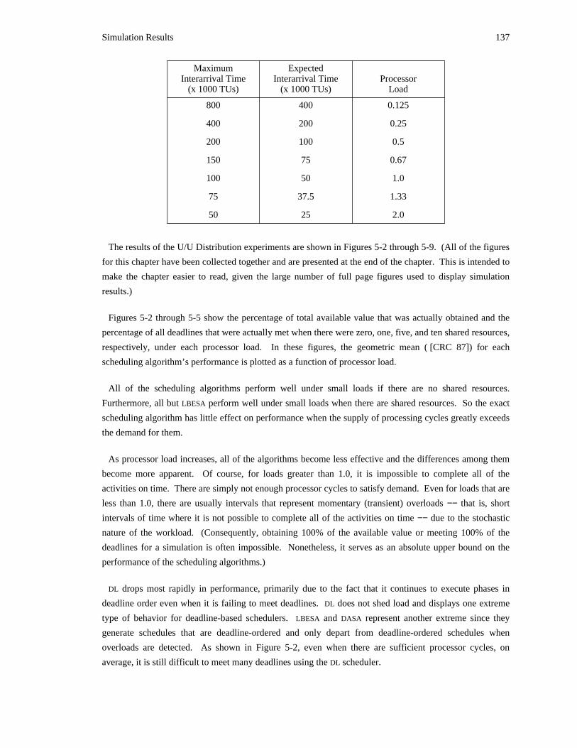
Simulation Results 137
Maximum ExpectedInterarrival Time Interarrival Time Processor
(x 1000 TUs) (x 1000 TUs) Load
800 400 0.125
400 200 0.25
200 100 0.5
150 75 0.67
100 50 1.0
75 37.5 1.33
50 25 2.0
The results of the U/U Distribution experiments are shown in Figures 5-2 through 5-9. (All of the figures
for this chapter have been collected together and are presented at the end of the chapter. This is intended to
make the chapter easier to read, given the large number of full page figures used to display simulation
results.)
Figures 5-2 through 5-5 show the percentage of total available value that was actually obtained and the
percentage of all deadlines that were actually met when there were zero, one, five, and ten shared resources,
respectively, under each processor load. In these figures, the geometric mean ( [CRC 87]) for each
scheduling algorithm’s performance is plotted as a function of processor load.
All of the scheduling algorithms perform well under small loads if there are no shared resources.
Furthermore, all but LBESA perform well under small loads when there are shared resources. So the exact
scheduling algorithm has little effect on performance when the supply of processing cycles greatly exceeds
the demand for them.
As processor load increases, all of the algorithms become less effective and the differences among them
become more apparent. Of course, for loads greater than 1.0, it is impossible to complete all of the
activities on time. There are simply not enough processor cycles to satisfy demand. Even for loads that are
less than 1.0, there are usually intervals that represent momentary (transient) overloads −− that is, short
intervals of time where it is not possible to complete all of the activities on time −− due to the stochastic
nature of the workload. (Consequently, obtaining 100% of the available value or meeting 100% of the
deadlines for a simulation is often impossible. Nonetheless, it serves as an absolute upper bound on the
performance of the scheduling algorithms.)
DL drops most rapidly in performance, primarily due to the fact that it continues to execute phases in
deadline order even when it is failing to meet deadlines. DL does not shed load and displays one extreme
type of behavior for deadline-based schedulers. LBESA and DASA represent another extreme since they
generate schedules that are deadline-ordered and only depart from deadline-ordered schedules when
overloads are detected. As shown in Figure 5-2, even when there are sufficient processor cycles, on
average, it is still difficult to meet many deadlines using the DL scheduler.
138 Scheduling Dependent Real-Time Activities
DL does not degrade appreciably with different numbers of shared resources because the poor overload
behavior just described dominates its performance. Since it was already missing most deadlines, adding
more constraints by requiring phases to acquire resources does not cause the application to miss many more
deadlines.
SPRI degrades smoothly as load increases. As more shared resources are added, increasing the interaction
of the activities, its performance decreases more rapidly as a function of load.
LBESA exhibits a few noteworthy tendencies. First of all, when there are no shared resources, it performs
almost exactly the same as DASA, surpassing both DL and SPRI under medium and high loads while
degrading gracefully. In fact, the lines plotting the performance of the two schedulers overlap and are
almost indistinguishable in both graphs in Figure 5-2.
When there are shared resources, LBESA performs quite differently. It typically performs much worse
than any of the other algorithms at relatively low processor loads. This results from a particularly
unfortunate interaction between LBESA and the shared resource manager.
As was pointed out in Section 1.1.1, the actions of the shared resource manager −− blocking executing
activities that request currently allocated resources and subsequently determining the order in which these
activities are again made ready to run (thus becoming visible to the scheduler again) −− constitute indirect
scheduling decisions.
The problem with LBESA and the resource manager arises when an activity requests a shared resource that
has previously been allocated to another activity. The requesting activity is then blocked and placed in a
FIFO queue to await its turn to access the resource. Later, the resource is allocated to the activity and the
activity is added to the ready list for the scheduler. However, if the activity fails to complete its current
phase −− either because there is insufficient time to complete it by its deadline or because it is shed in
response to an overload −− it will hold the resource indefinitely. Therefore, all activities that subsequently
require access to that resource will fail to meet their deadlines.
While the preceding scenario does not result every time an allocated shared resource is requested, it does
happen occasionally even at low processor loads.
DL and SPRI are not susceptible to this particular interaction because they never shed load. They
eventually execute every activity that arrives. Consequently, any activity that acquires a shared resource
will later complete execution of its current phase and release the resource. Only algorithms that shed load53must be concerned about the fact that activities that are shed may be holding shared resources .
53LBESA has been extensively modified to execute in the Alpha Operating System ( [Northcutt 87, Alpha 88, Alpha 90]). Severaladaptations were necessary to use the algorithm in Alpha. For instance, the Alpha programming model treats unsatisfied timeconstraints and communication failures, among others, as exceptions. When an exception is encountered, an associated handler isexecuted. This handler restores system data structures to acceptable states and offers the application programmer the opportunity todo the same for application data structures and activity state. This offers the opportunity to free shared resources in practice after anunsatisfied time constraint, even though the LBESA model does not address shared resources.
Simulation Results 139
In Figures 5-2 through 5-5, for any given scheduler operating with a specified number of resources, the
graph showing the mean value obtained as a function of processor load has a similar profile to the graph
showing the mean number of deadlines met. And typically, if one scheduler acquires more value at a
specific processor load than another scheduler, it also meets more deadlines. However, it is sometimes
possible to observe that schedulers place different emphasis on acquiring value and satisfying time
constraints. For example, at a processor load of 1.33 with either five or ten shared resources, LBESA, which
is explicitly concerned with time constraints, meets more deadlines than the value-driven SPRI scheduler,
but accrues less value.
DASA also degrades gracefully as processor load increases, managing to accrue more value and meet more
deadlines then any of the other algorithms in these simulations. Even with a load of 2.0, DASA obtains, on
average, around 60 percent or more of the available value −− almost 20 percent more value than any of the
other algorithms. (There is one exception. When there are no shared resources, DASA and LBESA exhibit
almost identical performance.)
DASA is not subject to an unfortunate interaction with the shared resource manager since it manages the
resources itself. Like LBESA, it will recognize that some activities holding shared resources cannot meet
their deadlines and so will not schedule them. However, unlike LBESA, DASA will realize when another
activity that can still meet its deadline needs the previously allocated resource and will attempt to execute
the activity holding the resource in order to enable continued progress by the application. In this way,
processor cycles are not consumed to free allocated resources unless there is an immediate need for the
resources. This is in keeping with the general philosophy that the system should always perform the
activities that will be most valuable to the system at any time −− processor cycles are not expended to free
allocated resources unless there is value in doing so (or unless there is literally nothing else to be done).
In Section 4.3.2.4, it was shown that if there were no shared resources DASA could accrue more value than
LBESA during overloads because LBESA could shed some activities unnecessarily. However, it would be
difficult, if not impossible, to prove analytically how often the conditions that are necessary for this
behavior to occur would arise during the execution of any given application. Fortunately, simulations of
general workloads or of specific applications can be used to gauge the magnitude of these behavioral
differences between DASA and LBESA.
The simulation results presented in Figure 5-2 show that this effect is quite small for this particular
workload. DASA and LBESA behave almost identically for all processor loads. In fact, for processor loads
of 0.5 or less, they perform identically. At loads of 1.0 or more, DASA outperforms LBESA by a narrow
margin −− from 0.01% to 0.17%. At a processor load of 0.67, LBESA acquires 0.01% more available value
than DASA. This is due to the fact that DASA is unable to utilize enough processor cycles during an overload
to justify using potential value density as the primary metric for ordering activities as they are added to the
tentative schedule. Under such circumstances, LBESA can utilize processor cycles (that were freed when it
unnecessarily shed some activities during overload) to run an activity with a lower potential value density
than DASA will run. If the activity selected by LBESA runs for a sufficiently long time, while DASA has
nothing left to execute after finishing the activities with higher potential value densities, LBESA can acquire
more value than DASA. (This scenario was outlined in Section 4.4.2.)
140 Scheduling Dependent Real-Time Activities
Figures 5-6 through 5-9 display more information concerning the U/U Distribution experiments. Where
Figures 5-2 through 5-5 plotted the geometric mean for each scheduling algorithm under various loads with
differing numbers of shared resources, Figures 5-6 through 5-9 show the range of values obtained and
deadlines met in each of these situations. In addition, the arithmetic mean is shown as a box placed along
the range; the geometric mean is shown as a star; and the harmonic mean is shown as a diamond. (The
definitions of the various means can be found in any standard statistical reference, such as [CRC 87].) As
always for nontrivial data sets, the arithmetic mean is greater than the geometric mean, which is greater
than the harmonic mean, for each case. However, the means are often so close that their symbols appear
superimposed in the figures.
In these figures, the x-axis again represents the nominal processor load. A group of four vertical lines
appears for each indicated load level, one line corresponding to each of the scheduling algorithms under
consideration. The groups are separated from one another by vertical dotted lines. The key, which appears
in each figure, indicates the line segment that corresponds to each scheduling algorithm within a group.
Specifically, the leftmost line segment displays the results for the deadline scheduler. To its right, are the
results for the static priority scheduler, then those for the LBESA scheduler, and finally the DASA scheduler
results. The top of the line segment for a given scheduler indicates the highest value obtained for the
displayed metric for any simulation run (at that processor load), and the bottom of the line segment
indicates the lowest value for the metric.
Once again, at low loads with no shared resources, all of the scheduling algorithms perform well,
displaying a fairly small variation in performance over multiple simulations. The introduction of shared
resources has a marked effect on LBESA’s performance, even at low loads −− it may perform as well as the
others or it may perform much worse (for reasons that were explained earlier in this section).
As load increases, each algorithm displays more variability across multiple simulations. Like LBESA at
lower loads, DL’s performance falls off sharply as load increases with a great deal of variability.
At higher loads, DASA’s performance is superior to the others. In fact, in several cases, the worst
performance by DASA for a given set of simulations is superior to the best performance of any of the other
algorithms. Furthermore, looking at individual simulations of high loads, DASA always performs as well as
any of the others, usually outperforming them.
5.2.3.3. Scheduler Performance Analysis: M/M Distribution
The M/M Distribution experiments feature activities that have interarrival times drawn from an
exponential probability distribution, where the experimenter specifies the mean interarrival time for any
given set of simulations. The mean interarrival time is varied to examine scheduler behavior under
different processor loads.
The deadline for each activity is also drawn from an exponential probability distribution with a mean
deadline of 100,000 TUs after activity arrival. This is the same expected time until deadline used for the
U/U Distribution experiments.
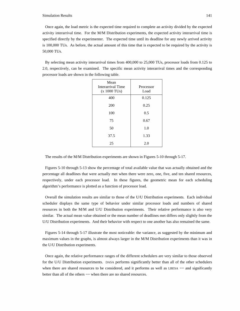
Simulation Results 141
Once again, the load metric is the expected time required to complete an activity divided by the expected
activity interarrival time. For the M/M Distribution experiments, the expected activity interarrival time is
specified directly by the experimenter. The expected time until its deadline for any newly arrived activity
is 100,000 TUs. As before, the actual amount of this time that is expected to be required by the activity is
50,000 TUs.
By selecting mean activity interarrival times from 400,000 to 25,000 TUs, processor loads from 0.125 to
2.0, respectively, can be examined. The specific mean activity interarrival times and the corresponding
processor loads are shown in the following table.
MeanInterarrival Time Processor
(x 1000 TUs) Load
400 0.125
200 0.25
100 0.5
75 0.67
50 1.0
37.5 1.33
25 2.0
The results of the M/M Distribution experiments are shown in Figures 5-10 through 5-17.
Figures 5-10 through 5-13 show the percentage of total available value that was actually obtained and the
percentage all deadlines that were actually met when there were zero, one, five, and ten shared resources,
respectively, under each processor load. In these figures, the geometric mean for each scheduling
algorithm’s performance is plotted as a function of processor load.
Overall the simulation results are similar to those of the U/U Distribution experiments. Each individual
scheduler displays the same type of behavior under similar processor loads and numbers of shared
resources in both the M/M and U/U Distribution experiments. Their relative performance is also very
similar. The actual mean value obtained or the mean number of deadlines met differs only slightly from the
U/U Distribution experiments. And their behavior with respect to one another has also remained the same.
Figures 5-14 through 5-17 illustrate the most noticeable: the variance, as suggested by the minimum and
maximum values in the graphs, is almost always larger in the M/M Distribution experiments than it was in
the U/U Distribution experiments.
Once again, the relative performance ranges of the different schedulers are very similar to those observed
for the U/U Distribution experiments. DASA performs significantly better than all of the other schedulers
when there are shared resources to be considered, and it performs as well as LBESA −− and significantly
better than all of the others −− when there are no shared resources.
142 Scheduling Dependent Real-Time Activities
Since the M/M Distribution experiments do exhibit a greater variance than the U/U Distribution
experiments, the M/M Distribution parameters were selected for use in the following experiments where
the amount of time spent making scheduling decisions is included in the simulations (Section 5.3) and the
benefit of issuing aborts to reduce the time required to free an allocated resource is analyzed (Section 5.4).
5.3. Evaluation of DASA With Scheduling Overhead
The analysis of DASA to this point has only evaluated the quality of decisions that can be made by
utilizing all of the information that is available to DASA. That is, the simulation results presented thus far
have assumed that each of the scheduling algorithms under investigation made its decisions
instantaneously.
In fact, each scheduler must consume resources −− in both time and space −− when making decisions.
Furthermore, complex schedulers, like DASA and LBESA, will require more time than simpler schedulers,
such as SPRI and DL.
In order to assess the efficacy of employing DASA in a real system, the time spent executing the
scheduling algorithm, which is referred to as the scheduling overhead, must be factored into the analysis
along with the time spent executing the application’s activities. The simulator can estimate the scheduling
overhead required for each individual decision made by each scheduler, and it can simulate the passage of
that amount of time as the simulation progresses.
Although the schedulers are different, they all spend a considerable amount of their execution time
performing a number of fundamental operations. These operations include list manipulations, arithmetic
operations, and entering and exiting the scheduler (or operating system). Consequently, the following
fundamental operations are monitored by the simulator as each scheduling algorithm executes:
• AddSubTime −− the amount of time required to add or subtract two floating point numbers;
• MultTime −− the amount of time required to multiply two floating point numbers;
• DivTime −− the amount of time required to divide one floating point number by another;
• SortFactor −− an amount of time that is used as a scaling factor when calculating the total timeto sort a list. For example, if a data structure and sort algorithm that require O(N log N) time tosort a list of N elements are used, the actual time consumed to sort an N element list is:SortFactor * N * (log N);
• InsDelFactor −− an amount of time that is used as a scaling factor when calculating the totaltime to insert an element into or delete it from a sorted list. For example, if a data structureand insert algorithm that require O(log N) time to insert an element into an ordered list of Nelements are used, the actual time consumed to insert the new element is: InsDelFactor * (logN);
• FixedOverheadTime −− the amount of time required to enter and exit the scheduler to executeits selection algorithm.
The time the scheduler consumes executing these operations is totaled by the simulator to yield the
scheduling overhead associated with any given scheduling decision.
By supplying values for each of these overhead parameters, the total overhead can be measured and its
Simulation Results 143
effects noted. As mentioned earlier (see Section 5.2.3.1), by having separate overhead parameters for these
fundamental scheduler operations, the effects of using different hardware support for schedulers or faster54implementations over time can be investigated .
One of the primary reasons to investigate the effects of scheduling overhead is to identify situations in
which the increased overhead incurred by using DASA is justified and also to identify those situations where
using DASA is impractical, given that the scheduler is executed on the same processor as the application.
Experiments were performed to investigate these issues. Once again, the M/M Distribution parameters
were used as a source for the simulation workload. This time only DASA, LBESA, and SPRI are compared.
(DL performed badly enough when overhead was not considered. Its performance only decreases when
overhead is included and so it is not an interesting algorithm at this stage.)
Experimentation led to the identification of three significant sets of values for the scheduling overhead
parameters. These sets of values differ by an order of magnitude from one to the next and correspond to
low, medium, and high overhead cases. The terms "low," "medium," and "high" are intended to denote the
fraction of the total available processor cycles that is spent executing DASA scheduler code. The time spent
executing DASA code is determined by several factors, including the quality of the DASA implementation,
the arrival rate of activities and their component phases, and the rate at which resource requests are made.
The effect of processor speed on the time taken to execute DASA code is accounted for in terms of the time
taken to execute each of the fundamental scheduling operations (expressed in TUs) when making a given
scheduling decision.
The experimental results, which will be presented in detail below, show that, under low overhead
conditions, DASA performs very nearly as well as it did in the experiments presented in Section 5.2, where
there was no overhead. When each fundamental scheduling operation is ten times more expensive, relative
to the time constraints governing the phases being scheduled, DASA still performs well, although the
additional overhead does degrade its performance somewhat. When the fundamental scheduling operations
are made ten times more expensive again, a point is reached at which nearly all of the processor’s cycles
are spent executing DASA, leaving few cycles for the application. (At the end of this section, these
overhead cases will be interpreted in terms of today’s technology.)
The values used for each fundamental scheduling operation parameter in each of the three overhead cases
are shown in the following table. Their relative values are meant to be suggestive of which operations
require more time, but are not intended to be extremely precise since great precision would be
implementation-dependent.
54To a great extent, this framework for expressing scheduling overhead is based on the use of traditional processors as executionengines for scheduling algorithms. Other possibilities exist, including the use of special-purpose scheduling processors. Variousscheduler optimizations for DASA are discussed further in Section 7.3.1.
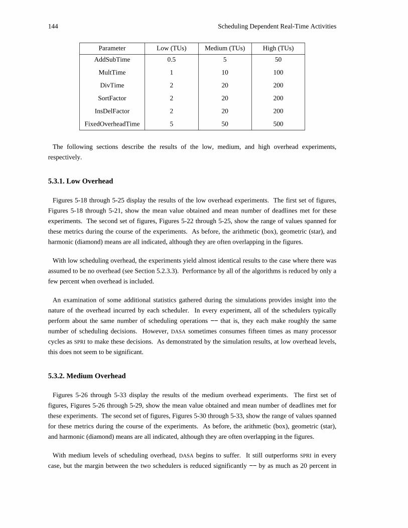
144 Scheduling Dependent Real-Time Activities
Parameter Low (TUs) Medium (TUs) High (TUs)
AddSubTime 0.5 5 50
MultTime 1 10 100
DivTime 2 20 200
SortFactor 2 20 200
InsDelFactor 2 20 200
FixedOverheadTime 5 50 500
The following sections describe the results of the low, medium, and high overhead experiments,
respectively.
5.3.1. Low Overhead
Figures 5-18 through 5-25 display the results of the low overhead experiments. The first set of figures,
Figures 5-18 through 5-21, show the mean value obtained and mean number of deadlines met for these
experiments. The second set of figures, Figures 5-22 through 5-25, show the range of values spanned for
these metrics during the course of the experiments. As before, the arithmetic (box), geometric (star), and
harmonic (diamond) means are all indicated, although they are often overlapping in the figures.
With low scheduling overhead, the experiments yield almost identical results to the case where there was
assumed to be no overhead (see Section 5.2.3.3). Performance by all of the algorithms is reduced by only a
few percent when overhead is included.
An examination of some additional statistics gathered during the simulations provides insight into the
nature of the overhead incurred by each scheduler. In every experiment, all of the schedulers typically
perform about the same number of scheduling operations −− that is, they each make roughly the same
number of scheduling decisions. However, DASA sometimes consumes fifteen times as many processor
cycles as SPRI to make these decisions. As demonstrated by the simulation results, at low overhead levels,
this does not seem to be significant.
5.3.2. Medium Overhead
Figures 5-26 through 5-33 display the results of the medium overhead experiments. The first set of
figures, Figures 5-26 through 5-29, show the mean value obtained and mean number of deadlines met for
these experiments. The second set of figures, Figures 5-30 through 5-33, show the range of values spanned
for these metrics during the course of the experiments. As before, the arithmetic (box), geometric (star),
and harmonic (diamond) means are all indicated, although they are often overlapping in the figures.
With medium levels of scheduling overhead, DASA begins to suffer. It still outperforms SPRI in every
case, but the margin between the two schedulers is reduced significantly −− by as much as 20 percent in
Simulation Results 145
some cases under heavy processor load. Most of the difference in the relative performance of these
schedulers is due to a decline by DASA. SPRI suffers only a slight loss in performance at this level of
scheduling overhead.
The reason that DASA is able to surpass SPRI is that: (1) under low processor load, there are sufficient
processor cycles to allow DASA to run without affecting the application’s activities to any great extent, and
(2) under high processor loads, there is a definite benefit to be gained by investing time in the scheduler,
thereby allowing it to carefully select what can feasibly be executed.
LBESA also declines slightly under medium levels of scheduling overhead, but not nearly as much as
DASA relative to its performance with low scheduling overhead. This is because, when shared resources are
involved, its behavior is dominated by its poor interaction with the resource manager. Therefore, although
its relative performance is fairly good as overhead levels increase from low to medium levels, its absolute
performance is not nearly so good.
5.3.3. High Overhead
Figures 5-34 through 5-41 display the results of the high overhead experiments. The first set of figures,
Figures 5-34 through 5-37, show the mean value obtained and mean number of deadlines met for these
experiments. The second set of figures, Figures 5-38 through 5-41, show the range of values spanned for
these metrics during the course of the experiments. As before, the arithmetic (box), geometric (star), and
harmonic (diamond) means are all indicated, although they are often overlapping in the figures.
With high scheduling overhead levels, it becomes impractical to execute DASA on the same processor as
the application. This is due to the fact that a large portion of the total processing time is spent executing the
scheduling algorithm, rather than the application’s activities. In fact, at high processor loads, in excess of
90 percent of the total processor time may be spent executing the scheduling algorithm. As a result, in
overload, when processor cycles are already in great demand, almost no cycles are available for the
application. Even at lower processor loads, the time spent executing the scheduling algorithm may be
around 20 percent of the total cycles actually needed to run the application.
5.3.4. Summary
The preceding simulation results demonstrate that DASA performs well and is preferred when there is low
to medium scheduling overhead in a uniprocessor system.
To put this into perspective, consider today’s technology. The time required to perform the arithmetic
scheduling operations is on the order of microseconds and the list manipulation scaling factors are on the
order of tens of microseconds. Also, assume that DASA becomes impractical at overhead levels just beyond
those of the medium overhead experiments. Then, by consulting the table of scheduling overhead
parameters presented in Section 5.3, it is seen that a TU is, according to today’s technology, somewhere
between 0.1 and 1.0 microsecond. Looking at the M/M Distribution parameters and U/U Distribution
146 Scheduling Dependent Real-Time Activities
parameters, it can be estimated that DASA is suitable for scheduling activities that have deadlines on the
order of tens or hundreds of milliseconds, even when each of these activities may require a substantial
portion of the available resources in that period of time. While this is certainly too slow for a number of
real-time applications, it is fast enough for a large number of supervisory control real-time applications, the
problem domain of interest for this work.
5.4. Evaluation of DASA Abort Usage
The concept of aborting a computational phase was included in the model for this research for two
reasons: (1) real supervisory control applications, as defined earlier, would need to be able to abort55computational phases in some situations −− to resolve a deadlock for instance ; and (2) some facilities,
particularly an atomic transaction facility designed to operate in a real-time environment, would regard the
ability to abort a phase as a primitive operation that is available to the facility.
Once the necessity of providing aborts is recognized, the possibility of further using them to the
application’s advantage in making scheduling decisions invites investigation. On the one hand, it seems
clear that aborting phases that hold shared resources reduces the length of time other phases must wait for
access to the resources. If the waiting phases are sufficiently time critical or valuable to the application,
then this reduced latency may be beneficial.
On the other hand, all of the processing cycles that had been consumed by an aborted phase have56effectively been wasted. They produced no value for the application . And, if the aborted phase’s
deadline may still be met, the phase may be reinitiated, consuming more processing cycles. Even if the
phase subsequently completes successfully, it will have consumed more cycles than it would have if there
were no aborts, contributing to a higher effective processor load.
DASA attempts to use aborts in a "greedy" manner, much like that just outlined to reduce the latency to
access a previously allocated resource. If a phase requires access to a resource held by another phase, DASA
will schedule the phase holding the resource so that it releases the resource as quickly as possible, based on
the information available to the scheduler at that time. Therefore, if it is quicker to abort a phase than to
complete it normally, an abort will be scheduled.
A series of experiments were performed to determine whether the reduced access latency, obtained at the
expense of reexecuting portions of some computational phases, resulted in an increase in accrued value for
55An unsatisfied time constraint provides another example where a real supervisory control system could benefit from the ability toissue an abort. Whenever a phase’s deadline is missed, it has only partially completed its task. This may produce a potentiallyinconsistent computational state, possibly mirrored by an inconsistent set of actions taken in the physical world. While these problemscan be ignored in a simulated system, in an actual implementation, steps would have to be taken to ensure that computational andphysical resources were in acceptable states before they could be used again. An abort mechanism provides a straightforward methodto accomplish the necessary actions to restore order to the affected resources.
56Under the model presented in this thesis, aborted phases produce no value for the application. There are situations, however,where this may not be the case. For example, if iterative solution techniques are used to solve a problem, an aborted computationcould yield a partial result that does contribute some value to the application. The present model may be enhanced to encompass suchpossibilities in the future.
Simulation Results 147
the application. These simulations, like many of the previous experiments presented in this chapter, used
the M/M Distribution parameters. In addition, the experiments were done for each of the three levels of
scheduling overhead investigated in Section 5.3. Thus, the results should represent behavior in realistic
scenarios.
Only the DASA scheduler is used in these experiments, since it is the only algorithm that may issue aborts.
For each simulation, two different scenarios were used. The DASA algorithm is exactly the same in both
cases. In the first case, each shared resource is assigned an undo time that is (essentially) infinite.
Consequently, it will never be quicker to abort a phase than to complete it normally, and no aborts will be
issued. In the second case, each shared resource is assigned an undo time of 100 TUs. This is sufficiently
low, compared to the time constraints the activities must satisfy, to allow the scheduler to occasionally
abort a phase.
The results of the experiments are shown in Figures 5-42 through 5-50. The first three figures show the
performance for DASA when there is a single shared resource under low, medium, and high levels of
scheduling overhead, respectively. The second set of three figures presents the same type of information
when there are five shared resources. And the last three figures display the results of experiments utilizing
ten shared resources.
No simulations were done for scenarios where there were no shared resources, since, without resource
conflicts, there is no opportunity to abort phases.
In general, the use of aborts benefits the application when scheduling overhead is at low or medium
levels. In these cases, the application accrues more value and meets more deadlines when DASA issues
aborts than when it does not.
The benefits gained from issuing aborts are more pronounced at higher processor utilization levels and
also with greater numbers of shared resources. (Remember that, given the experimental workload, an
increase in the number of shared resources brings with it a substantial increase in the number of shared
resource requests.) At low processor loads and low scheduling overhead, an application may accrue a few
percent more value by employing aborts. At higher processing loads and medium scheduling overhead, a
benefit of ten percent or more may result from the use of aborts by the scheduler.
For completeness, results are shown for simulations featuring high levels of scheduling overhead. The
use of aborts provides no great difference in these situations. DASA performs poorly in either case and is
not appropriate for use in such circumstances.
An examination of the event logs of these simulations yields a few noteworthy observations. First of all,
aborted computational phases, although they are always restarted, are often never completed successfully.
Usually, they are too close to their deadline to successfully meet it or have a lower potential value density
than other candidate phases. Second, despite the fact that many of the aborted phases never complete
successfully, some do. In fact, there were simulations in which a phase was aborted twice, blocked on
entry each time it was restarted, and preempted by another phase before it completed, meeting its deadline.
148 Scheduling Dependent Real-Time Activities
Finally, if the set of phases that complete successfully for a simulation where DASA issues aborts is
compared to the set of phases that complete successfully when it does not, it is not unusual to observe
significant differences. While there is always a substantial overlap in these sets, the actual identities of the
completed phases differs more than the experimental results may imply. For example, if issuing aborts
results in meeting three percent more deadlines than not issuing aborts for a given simulation, the two sets
of completed phases may share only 85 or 90 percent of their members. Put another way, they may differ
in 10 to 15 percent of their membership.
5.5. Interpreting Simulation Results for Specific Applications
To complete this chapter, this section looks at two supervisory control applications for which DASA may
be useful. While they are indicative of classes of applications that might be of interest, they do not touch
on many other possibilities, such as simulators and military platform management.
These applications are discussed for two reasons. First of all, they give a flavor of some other
applications (in addition to those presented in Chapter 1). The characteristics that make these applications
particularly amenable to the use of the DASA scheduling algorithm are noted where appropriate.
Secondly, they offer a chance to use real applications to study how the metrics used for the simulation
results can be initially estimated from a knowledge of the application. Of course, the applications are
presented briefly here and better statistics could be carefully gathered by researchers or real-time system
professionals who were interested in investigating alternate scheduling algorithms for a specific
application.
Each application is outlined briefly, roughly indicating the types of time constraints involved, the
processing requirements, and the number and types of shared resources. Application details are provided to
explain how supervisory control system requirements are shaped by the physical world. However, the
descriptions are necessarily brief since too many details would obscure the important information
concerning application structure and requirements.
5.5.1. Telephone Switching
The telephone company typically creates a dedicated circuit to handle each telephone call. This circuit is
actually composed of a number of shorter circuits that are connected by computer-controlled switches.
These switches handle the routing of the call from the originator to the receiver.
Each time a call is initiated, a circuit must be set up to complete the call. At each routing switch along the
way, signals must be sent and acknowledged in a moderately short period of time −− often on the order of a
second.
Because there is no way to associate a priority with a call, it is generally impossible to distinguish urgent
calls from less important calls. Therefore, a certain portion of the circuit capacity of the phone company is
Simulation Results 149
often held in reserve, even during periods of peak demand, in order to service critical calls in case of an
emergency. As a result, this capacity is unavailable for general service and is wasted (in a sense) when
there are no emergency calls.
This application could almost certainly benefit by using a scheduling algorithm such as DASA. For57instance, the application could be restructured so that each call had an associated priority . As indicated
earlier, each call also has a series of time constraints that must be met in order to properly control the
switches needed to complete the call. So the simple time-value functions used in this research can be
applied directly in this application to capture both the importance and the urgency of each call in the
system. So an activity can be assigned to handle each call.
The shared resources in the system are the circuits and switch connections. To complete a call a number
of these shared resources must be acquired. At the completion of the call, they may be released.
In addition, no circuits must be reserved exclusively for emergency calls. Therefore, the overall capacity
for telephone calls available to telephone company subscribers can be increased. This is due to the
behavior of DASA under overload conditions.
Under normal conditions, where there are sufficient resources exist to satisfy demands in a timely
manner, all of the calls are completed and activities are scheduled essentially in order of their respective
deadlines regardless of their relative priorities. When demand exceeds the supply of shared resources (even
within a single switch), some calls cannot be completed. In that case, a call’s priority would be considered
when making scheduling decisions so that more important calls receive shared resources at the expense of
less important calls. In fact, DASA would abort less important calls that are holding shared resources in58order to free circuits and switches to complete new, higher priority calls .
The transition from overload to normal (non-overload) processing would be as graceful as the
transformation into the overload case, where most parties are likely to be uneffected while emergency
traffic acquires the resources it needs.
There are a wealth of statistics available to the telephone companies describing the frequency at which
calls arrive throughout a day, profiling various days (weekends, weekdays, Mother’s Day, and so on), the
computational requirements to route a call and to make the necessary connections, and the numbers and
types of the shared resources in the system (circuits, switch connections, logs, and databases for instance).
57This priority could be associated with the physical phone line on which the call originates or it could be associated with the typeof call being made (emergency numbers or signals could have high priorities, for example).
58While aborting any calls is unfortunate −− they represent a disruption of service to customers −− these aborts will not entailserious damage. More likely, an abort will result in a disgruntled caller and callee. And since humans are involved in virtually everycall, they are capable of taking appropriate steps following an aborted call −− perhaps redialing immediately, maybe waiting awhilebefore redialing, or maybe just waiting for a more opportune time if the call was not at all urgent. The actual abort processing presentsthe telephone company with an opportunity to make the abort in a fairly painless way. As the connection is broken, each party in thecall could be informed that the call had to be aborted in favor of an urgent call. Furthermore, the affected parties could be given somecompensation for their inconvenience such as an account credit or a free call at a later date. The processing requirements for this typeof abort processing could be associated with the acquisition of circuits and switch connections and is accommodated by the abortmodel for this research, which allows a resource-dependent amount of processing time to be reserved in case an abort occurs.
150 Scheduling Dependent Real-Time Activities
These statistics would be used to consult the simulation charts presented in this chapter or others derived
for this specific application.
Although this example discussed the public telephone system, the use of a priority switching service
seems to have even greater potential in other applications, both industrial and military, where dedicated
communication networks can be employed.
5.5.2. Process Control: A Steel Mill
A steel mill provides a number of supervisory control applications that could benefit from advantageous
real-time scheduling. This section returns to the example that was originally introduced in Sections 1.1.2
and 1.4, focusing on a computer system that controls a number of furnaces supplying steel with specific
chemical compositions to a pair of continuous casters, which cast the molten steel into slabs. (This is
similar to the supervisory control system described in [DEI 85].)
First, consider some of the time constraints for this application.
Each caster continuously produces a slab that is cut to specified lengths to fill orders. The slab lengths
typically vary between twenty and forty feet, and each time a new slab is cut, a new slab record has to be
generated and stored.
The caster speed varies −− if it moves too quickly, the metal will not have solidified sufficiently by the
time it emerges from the caster; if it moves too slowly, productivity will be unnecessarily low. The caster
is operated at the maximum speed at which solid steel can be produced. This speed is determined by the
temperature and chemistry of the steel being cast, the water temperature and spray rates of cooling nozzles
located along the length of the caster, and several other factors. Typically, a new foot of steel emerges
from the caster every six to twelve seconds.
Each time a new foot of steel is cast, a record must be created to document the chemistry of the foot and
other information that is used to track the metal through the mill. If this information is lost or is not
recorded on time, the chemistry of the slab cannot be adequately certified for customers with strict product
quality requirements, and the slab cannot be sold to them. The processing that occurs as each foot of steel
is cast is quite complex and requires a second or two of processing time.
The furnace has fewer tight time constraints than the caster. The furnaces produce steel in units called
"heats." A heat typically requires between thirty and forty-five minutes to produce. During that time, the
chemistry of the steel is calculated several times by a complex analytical model. The chemistry is also
measured directly by a chemistry laboratory. Even after the heat is produced the steel’s composition may
be adjusted at a liquid metallurgy facility. Near the conclusion of a heat, oxygen is blown through the
molten metal to reduce the carbon content of the steel. It is important to produce steel with a fairly precise
carbon content because of the extent to which carbon content affects the physical properties of steel. The
oxygen is blown through the steel under the direction of the supervisory control computer, and it must be
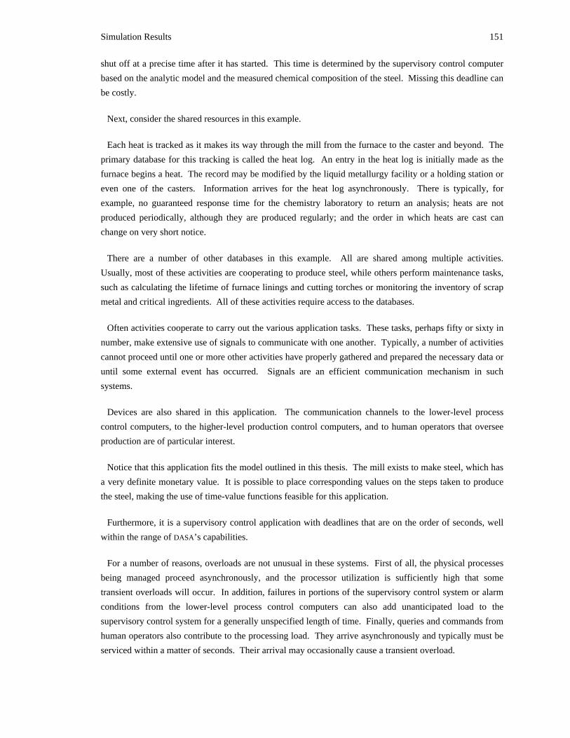
Simulation Results 151
shut off at a precise time after it has started. This time is determined by the supervisory control computer
based on the analytic model and the measured chemical composition of the steel. Missing this deadline can
be costly.
Next, consider the shared resources in this example.
Each heat is tracked as it makes its way through the mill from the furnace to the caster and beyond. The
primary database for this tracking is called the heat log. An entry in the heat log is initially made as the
furnace begins a heat. The record may be modified by the liquid metallurgy facility or a holding station or
even one of the casters. Information arrives for the heat log asynchronously. There is typically, for
example, no guaranteed response time for the chemistry laboratory to return an analysis; heats are not
produced periodically, although they are produced regularly; and the order in which heats are cast can
change on very short notice.
There are a number of other databases in this example. All are shared among multiple activities.
Usually, most of these activities are cooperating to produce steel, while others perform maintenance tasks,
such as calculating the lifetime of furnace linings and cutting torches or monitoring the inventory of scrap
metal and critical ingredients. All of these activities require access to the databases.
Often activities cooperate to carry out the various application tasks. These tasks, perhaps fifty or sixty in
number, make extensive use of signals to communicate with one another. Typically, a number of activities
cannot proceed until one or more other activities have properly gathered and prepared the necessary data or
until some external event has occurred. Signals are an efficient communication mechanism in such
systems.
Devices are also shared in this application. The communication channels to the lower-level process
control computers, to the higher-level production control computers, and to human operators that oversee
production are of particular interest.
Notice that this application fits the model outlined in this thesis. The mill exists to make steel, which has
a very definite monetary value. It is possible to place corresponding values on the steps taken to produce
the steel, making the use of time-value functions feasible for this application.
Furthermore, it is a supervisory control application with deadlines that are on the order of seconds, well
within the range of DASA’s capabilities.
For a number of reasons, overloads are not unusual in these systems. First of all, the physical processes
being managed proceed asynchronously, and the processor utilization is sufficiently high that some
transient overloads will occur. In addition, failures in portions of the supervisory control system or alarm
conditions from the lower-level process control computers can also add unanticipated load to the
supervisory control system for a generally unspecified length of time. Finally, queries and commands from
human operators also contribute to the processing load. They arrive asynchronously and typically must be
serviced within a matter of seconds. Their arrival may occasionally cause a transient overload.
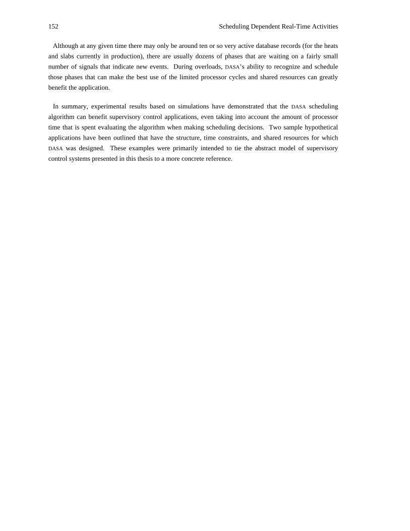
152 Scheduling Dependent Real-Time Activities
Although at any given time there may only be around ten or so very active database records (for the heats
and slabs currently in production), there are usually dozens of phases that are waiting on a fairly small
number of signals that indicate new events. During overloads, DASA’s ability to recognize and schedule
those phases that can make the best use of the limited processor cycles and shared resources can greatly
benefit the application.
In summary, experimental results based on simulations have demonstrated that the DASA scheduling
algorithm can benefit supervisory control applications, even taking into account the amount of processor
time that is spent evaluating the algorithm when making scheduling decisions. Two sample hypothetical
applications have been outlined that have the structure, time constraints, and shared resources for which
DASA was designed. These examples were primarily intended to tie the abstract model of supervisory
control systems presented in this thesis to a more concrete reference.
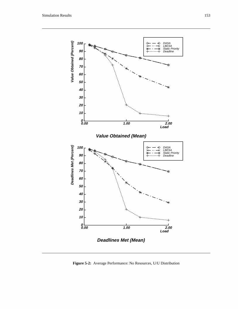
Simulation Results 153
0
10
20
30
40
50
60
70
80
90
100
Val
ue
Ob
tain
ed (
Per
cen
t)
0.00 1.00 2.00Load
Value Obtained (Mean)
DeadlineStatic PriorityLBESADASA
0
10
20
30
40
50
60
70
80
90
100
Dea
dlin
es M
et (
Per
cen
t)
0.00 1.00 2.00Load
Deadlines Met (Mean)
DeadlineStatic PriorityLBESADASA
Figure 5-2: Average Performance: No Resources, U/U Distribution
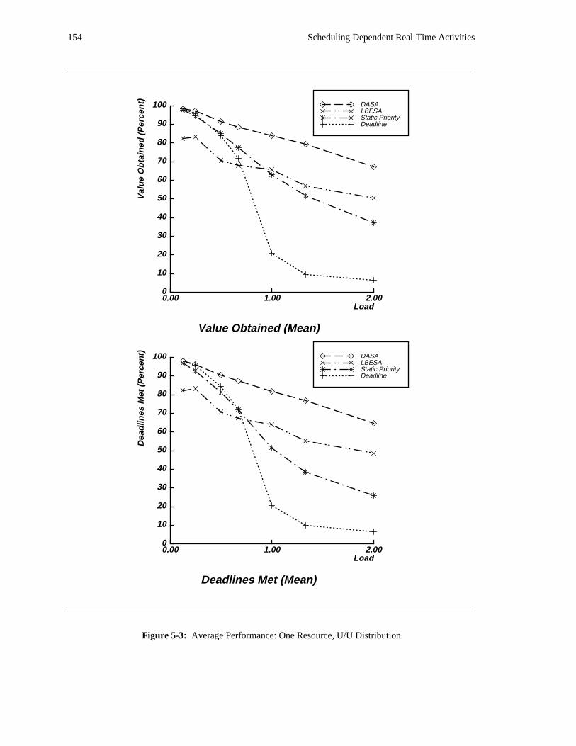
154 Scheduling Dependent Real-Time Activities
0
10
20
30
40
50
60
70
80
90
100
Val
ue
Ob
tain
ed (
Per
cen
t)
0.00 1.00 2.00Load
Value Obtained (Mean)
DeadlineStatic PriorityLBESADASA
0
10
20
30
40
50
60
70
80
90
100
Dea
dlin
es M
et (
Per
cen
t)
0.00 1.00 2.00Load
Deadlines Met (Mean)
DeadlineStatic PriorityLBESADASA
Figure 5-3: Average Performance: One Resource, U/U Distribution
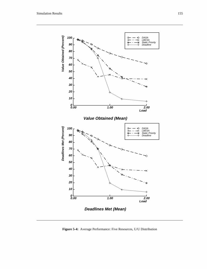
Simulation Results 155
0
10
20
30
40
50
60
70
80
90
100
Val
ue
Ob
tain
ed (
Per
cen
t)
0.00 1.00 2.00Load
Value Obtained (Mean)
DeadlineStatic PriorityLBESADASA
0
10
20
30
40
50
60
70
80
90
100
Dea
dlin
es M
et (
Per
cen
t)
0.00 1.00 2.00Load
Deadlines Met (Mean)
DeadlineStatic PriorityLBESADASA
Figure 5-4: Average Performance: Five Resources, U/U Distribution
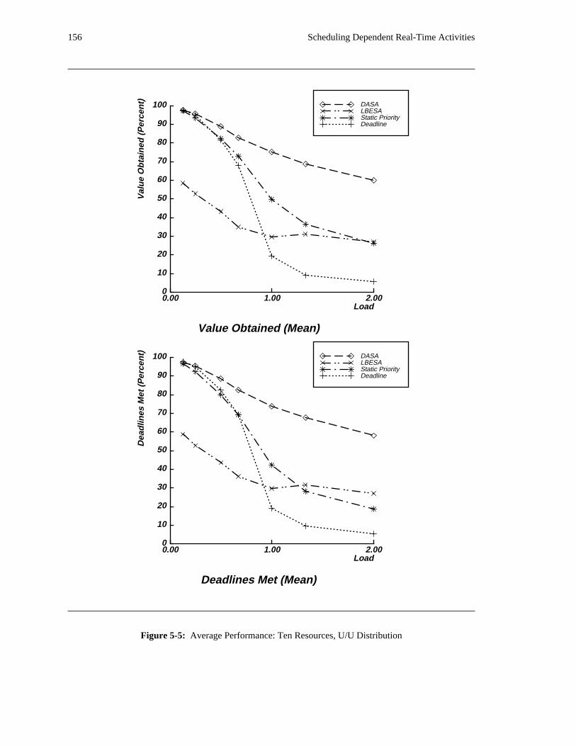
156 Scheduling Dependent Real-Time Activities
0
10
20
30
40
50
60
70
80
90
100
Val
ue
Ob
tain
ed (
Per
cen
t)
0.00 1.00 2.00Load
Value Obtained (Mean)
DeadlineStatic PriorityLBESADASA
0
10
20
30
40
50
60
70
80
90
100
Dea
dlin
es M
et (
Per
cen
t)
0.00 1.00 2.00Load
Deadlines Met (Mean)
DeadlineStatic PriorityLBESADASA
Figure 5-5: Average Performance: Ten Resources, U/U Distribution
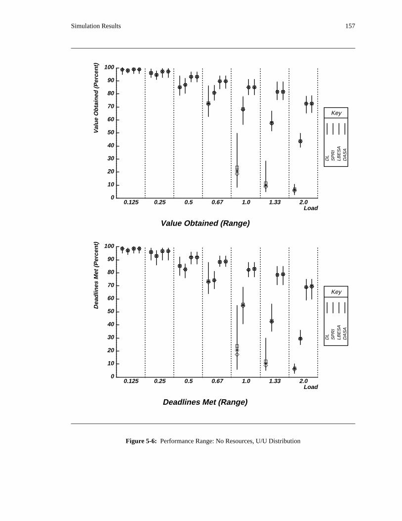
Simulation Results 157
Key
DL
SP
RI
LBE
SA
DA
SA
0
10
20
30
40
50
60
70
80
90
100
Val
ue
Ob
tain
ed (
Per
cen
t)
Load
Value Obtained (Range)
0.125 0.25 0.5 0.67 1.0 1.33 2.0
Key
DL
SP
RI
LBE
SA
DA
SA
0
10
20
30
40
50
60
70
80
90
100
Dea
dlin
es M
et (
Per
cen
t)
Load
Deadlines Met (Range)
0.125 0.25 0.5 0.67 1.0 1.33 2.0
Figure 5-6: Performance Range: No Resources, U/U Distribution
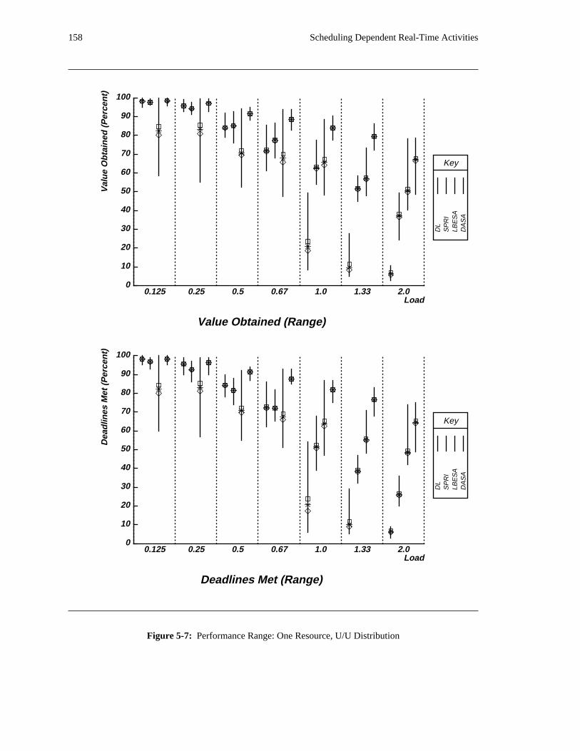
158 Scheduling Dependent Real-Time Activities
Key
DL
SP
RI
LBE
SA
DA
SA
0
10
20
30
40
50
60
70
80
90
100V
alu
e O
bta
ined
(P
erce
nt)
Load
Value Obtained (Range)
0.125 0.25 0.5 0.67 1.0 1.33 2.0
Key
DL
SP
RI
LBE
SA
DA
SA
0
10
20
30
40
50
60
70
80
90
100
Dea
dlin
es M
et (
Per
cen
t)
Load
Deadlines Met (Range)
0.125 0.25 0.5 0.67 1.0 1.33 2.0
Figure 5-7: Performance Range: One Resource, U/U Distribution
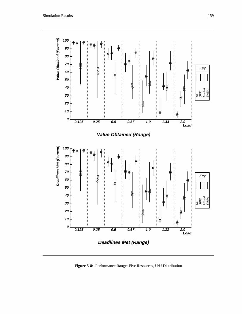
Simulation Results 159
Key
DL
SP
RI
LBE
SA
DA
SA
0
10
20
30
40
50
60
70
80
90
100
Val
ue
Ob
tain
ed (
Per
cen
t)
Load
Value Obtained (Range)
0.125 0.25 0.5 0.67 1.0 1.33 2.0
Key
DL
SP
RI
LBE
SA
DA
SA
0
10
20
30
40
50
60
70
80
90
100
Dea
dlin
es M
et (
Per
cen
t)
Load
Deadlines Met (Range)
0.125 0.25 0.5 0.67 1.0 1.33 2.0
Figure 5-8: Performance Range: Five Resources, U/U Distribution
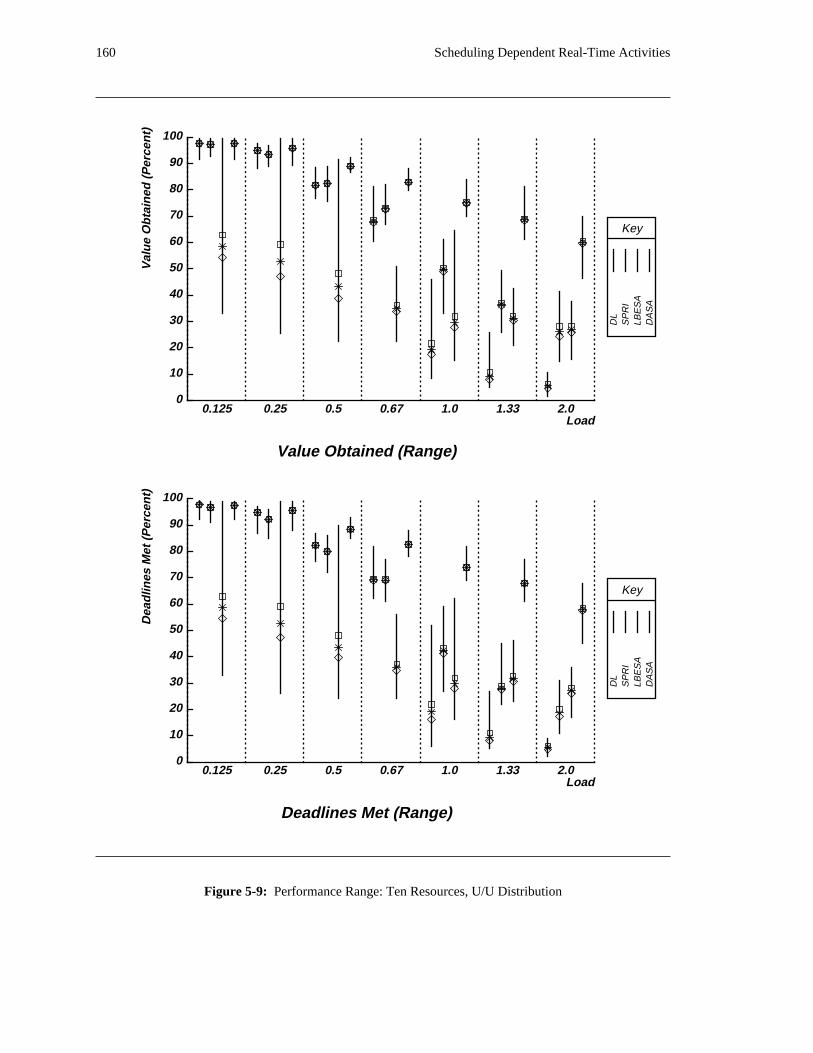
160 Scheduling Dependent Real-Time Activities
Key
DL
SP
RI
LBE
SA
DA
SA
0
10
20
30
40
50
60
70
80
90
100V
alu
e O
bta
ined
(P
erce
nt)
Load
Value Obtained (Range)
0.125 0.25 0.5 0.67 1.0 1.33 2.0
Key
DL
SP
RI
LBE
SA
DA
SA
0
10
20
30
40
50
60
70
80
90
100
Dea
dlin
es M
et (
Per
cen
t)
Load
Deadlines Met (Range)
0.125 0.25 0.5 0.67 1.0 1.33 2.0
Figure 5-9: Performance Range: Ten Resources, U/U Distribution
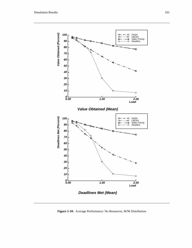
Simulation Results 161
0
10
20
30
40
50
60
70
80
90
100
Val
ue
Ob
tain
ed (
Per
cen
t)
0.00 1.00 2.00Load
Value Obtained (Mean)
DeadlineStatic PriorityLBESADASA
0
10
20
30
40
50
60
70
80
90
100
Dea
dlin
es M
et (
Per
cen
t)
0.00 1.00 2.00Load
Deadlines Met (Mean)
DeadlineStatic PriorityLBESADASA
Figure 5-10: Average Performance: No Resources, M/M Distribution
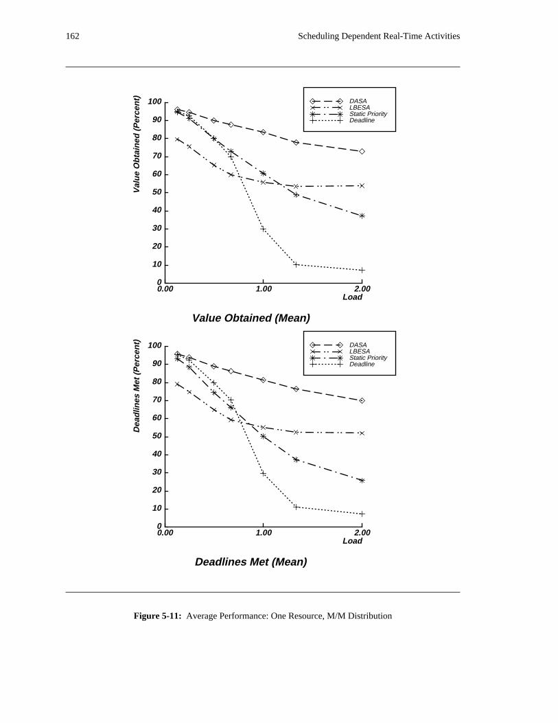
162 Scheduling Dependent Real-Time Activities
0
10
20
30
40
50
60
70
80
90
100
Val
ue
Ob
tain
ed (
Per
cen
t)
0.00 1.00 2.00Load
Value Obtained (Mean)
DeadlineStatic PriorityLBESADASA
0
10
20
30
40
50
60
70
80
90
100
Dea
dlin
es M
et (
Per
cen
t)
0.00 1.00 2.00Load
Deadlines Met (Mean)
DeadlineStatic PriorityLBESADASA
Figure 5-11: Average Performance: One Resource, M/M Distribution
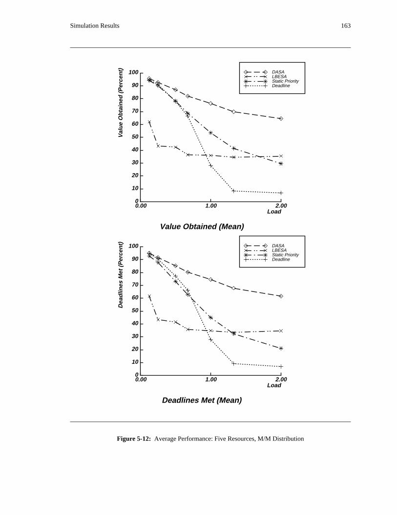
Simulation Results 163
0
10
20
30
40
50
60
70
80
90
100
Val
ue
Ob
tain
ed (
Per
cen
t)
0.00 1.00 2.00Load
Value Obtained (Mean)
DeadlineStatic PriorityLBESADASA
0
10
20
30
40
50
60
70
80
90
100
Dea
dlin
es M
et (
Per
cen
t)
0.00 1.00 2.00Load
Deadlines Met (Mean)
DeadlineStatic PriorityLBESADASA
Figure 5-12: Average Performance: Five Resources, M/M Distribution
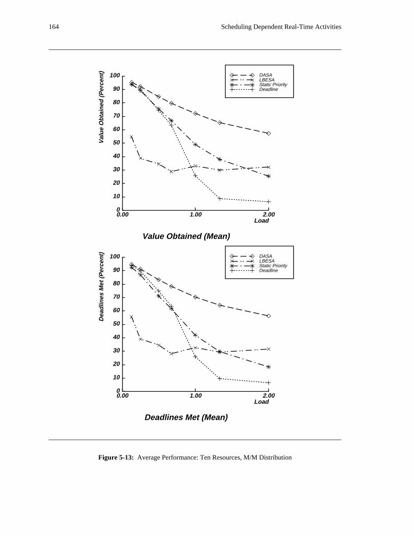
164 Scheduling Dependent Real-Time Activities
0
10
20
30
40
50
60
70
80
90
100
Val
ue
Ob
tain
ed (
Per
cen
t)
0.00 1.00 2.00Load
Value Obtained (Mean)
DeadlineStatic PriorityLBESADASA
0
10
20
30
40
50
60
70
80
90
100
Dea
dlin
es M
et (
Per
cen
t)
0.00 1.00 2.00Load
Deadlines Met (Mean)
DeadlineStatic PriorityLBESADASA
Figure 5-13: Average Performance: Ten Resources, M/M Distribution
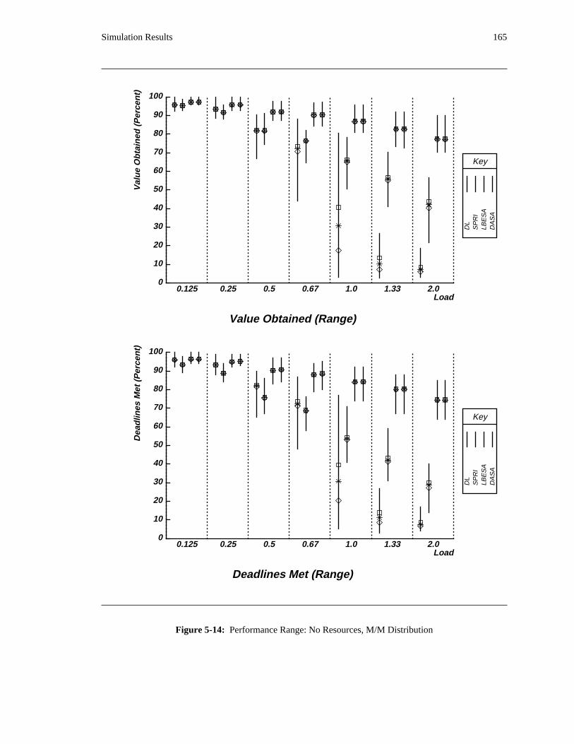
Simulation Results 165
Key
DL
SP
RI
LBE
SA
DA
SA
0
10
20
30
40
50
60
70
80
90
100
Val
ue
Ob
tain
ed (
Per
cen
t)
Load
Value Obtained (Range)
0.125 0.25 0.5 0.67 1.0 1.33 2.0
Key
DL
SP
RI
LBE
SA
DA
SA
0
10
20
30
40
50
60
70
80
90
100
Dea
dlin
es M
et (
Per
cen
t)
Load
Deadlines Met (Range)
0.125 0.25 0.5 0.67 1.0 1.33 2.0
Figure 5-14: Performance Range: No Resources, M/M Distribution
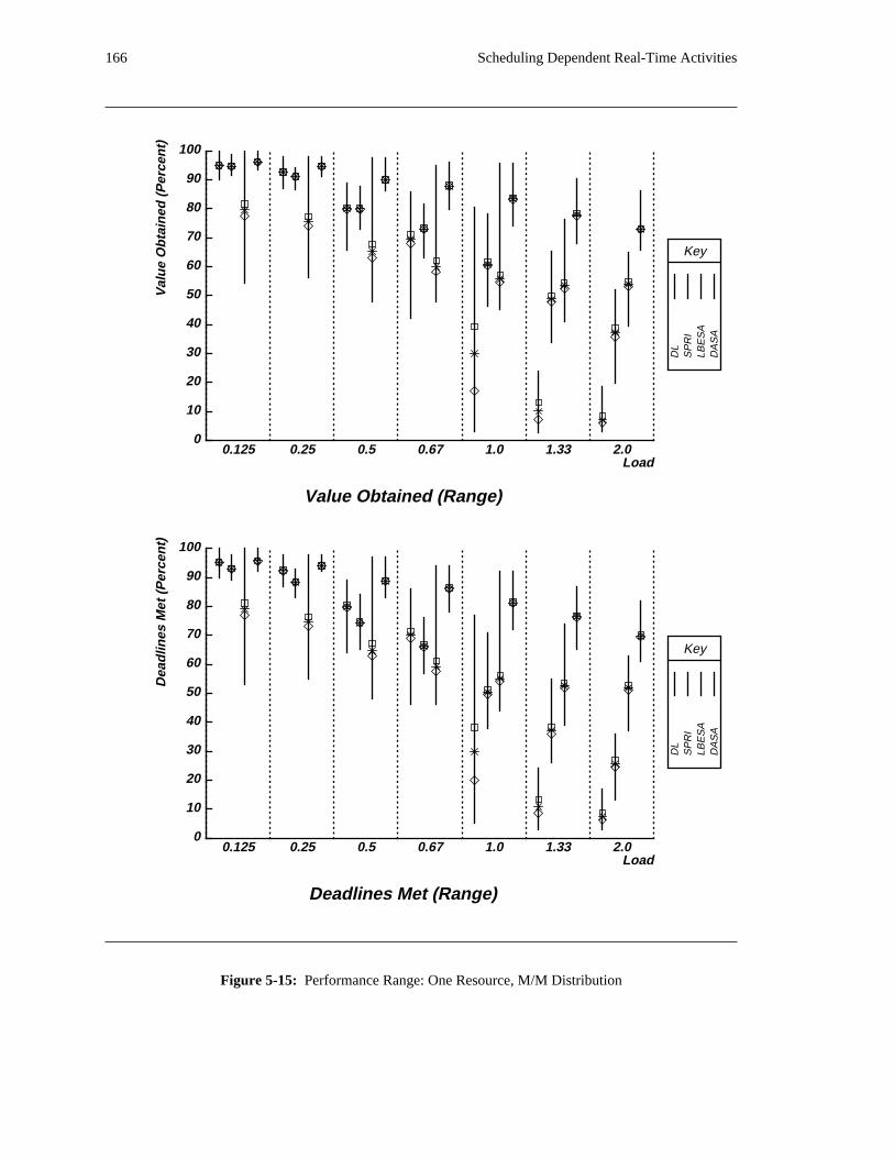
166 Scheduling Dependent Real-Time Activities
Key
DL
SP
RI
LBE
SA
DA
SA
0
10
20
30
40
50
60
70
80
90
100V
alu
e O
bta
ined
(P
erce
nt)
Load
Value Obtained (Range)
0.125 0.25 0.5 0.67 1.0 1.33 2.0
Key
DL
SP
RI
LBE
SA
DA
SA
0
10
20
30
40
50
60
70
80
90
100
Dea
dlin
es M
et (
Per
cen
t)
Load
Deadlines Met (Range)
0.125 0.25 0.5 0.67 1.0 1.33 2.0
Figure 5-15: Performance Range: One Resource, M/M Distribution
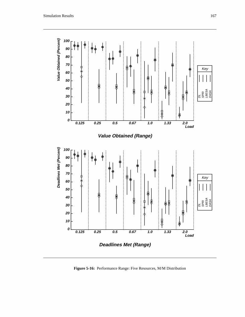
Simulation Results 167
Key
DL
SP
RI
LBE
SA
DA
SA
0
10
20
30
40
50
60
70
80
90
100
Val
ue
Ob
tain
ed (
Per
cen
t)
Load
Value Obtained (Range)
0.125 0.25 0.5 0.67 1.0 1.33 2.0
Key
DL
SP
RI
LBE
SA
DA
SA
0
10
20
30
40
50
60
70
80
90
100
Dea
dlin
es M
et (
Per
cen
t)
Load
Deadlines Met (Range)
0.125 0.25 0.5 0.67 1.0 1.33 2.0
Figure 5-16: Performance Range: Five Resources, M/M Distribution
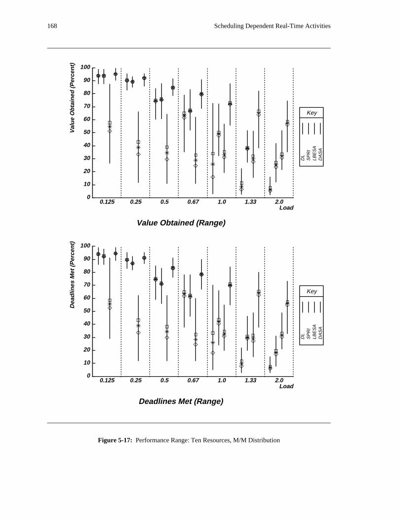
168 Scheduling Dependent Real-Time Activities
Key
DL
SP
RI
LBE
SA
DA
SA
0
10
20
30
40
50
60
70
80
90
100V
alu
e O
bta
ined
(P
erce
nt)
Load
Value Obtained (Range)
0.125 0.25 0.5 0.67 1.0 1.33 2.0
Key
DL
SP
RI
LBE
SA
DA
SA
0
10
20
30
40
50
60
70
80
90
100
Dea
dlin
es M
et (
Per
cen
t)
Load
Deadlines Met (Range)
0.125 0.25 0.5 0.67 1.0 1.33 2.0
Figure 5-17: Performance Range: Ten Resources, M/M Distribution
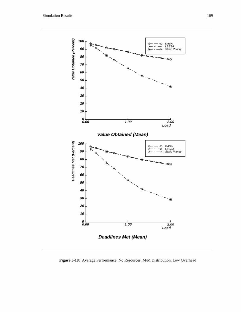
Simulation Results 169
0
10
20
30
40
50
60
70
80
90
100
Val
ue
Ob
tain
ed (
Per
cen
t)
0.00 1.00 2.00Load
Value Obtained (Mean)
Static PriorityLBESADASA
0
10
20
30
40
50
60
70
80
90
100
Dea
dlin
es M
et (
Per
cen
t)
0.00 1.00 2.00Load
Deadlines Met (Mean)
Static PriorityLBESADASA
Figure 5-18: Average Performance: No Resources, M/M Distribution, Low Overhead
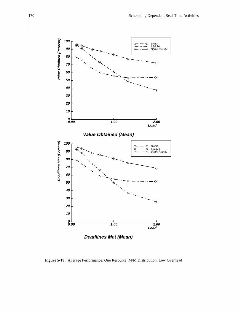
170 Scheduling Dependent Real-Time Activities
0
10
20
30
40
50
60
70
80
90
100
Val
ue
Ob
tain
ed (
Per
cen
t)
0.00 1.00 2.00Load
Value Obtained (Mean)
Static PriorityLBESADASA
0
10
20
30
40
50
60
70
80
90
100
Dea
dlin
es M
et (
Per
cen
t)
0.00 1.00 2.00Load
Deadlines Met (Mean)
Static PriorityLBESADASA
Figure 5-19: Average Performance: One Resource, M/M Distribution, Low Overhead
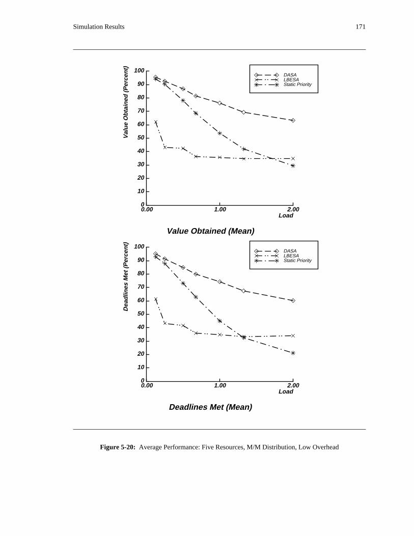
Simulation Results 171
0
10
20
30
40
50
60
70
80
90
100
Val
ue
Ob
tain
ed (
Per
cen
t)
0.00 1.00 2.00Load
Value Obtained (Mean)
Static PriorityLBESADASA
0
10
20
30
40
50
60
70
80
90
100
Dea
dlin
es M
et (
Per
cen
t)
0.00 1.00 2.00Load
Deadlines Met (Mean)
Static PriorityLBESADASA
Figure 5-20: Average Performance: Five Resources, M/M Distribution, Low Overhead
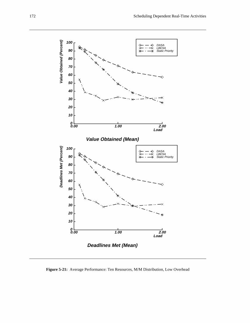
172 Scheduling Dependent Real-Time Activities
0
10
20
30
40
50
60
70
80
90
100
Val
ue
Ob
tain
ed (
Per
cen
t)
0.00 1.00 2.00Load
Value Obtained (Mean)
Static PriorityLBESADASA
0
10
20
30
40
50
60
70
80
90
100
Dea
dlin
es M
et (
Per
cen
t)
0.00 1.00 2.00Load
Deadlines Met (Mean)
Static PriorityLBESADASA
Figure 5-21: Average Performance: Ten Resources, M/M Distribution, Low Overhead
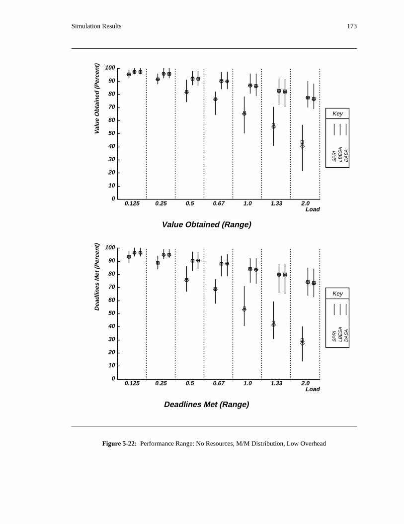
Simulation Results 173
Key
SP
RI
LBE
SA
DA
SA
0
10
20
30
40
50
60
70
80
90
100
Val
ue
Ob
tain
ed (
Per
cen
t)
Load
Value Obtained (Range)
0.125 0.25 0.5 0.67 1.0 1.33 2.0
Key
SP
RI
LBE
SA
DA
SA
0
10
20
30
40
50
60
70
80
90
100
Dea
dlin
es M
et (
Per
cen
t)
Load
Deadlines Met (Range)
0.125 0.25 0.5 0.67 1.0 1.33 2.0
Figure 5-22: Performance Range: No Resources, M/M Distribution, Low Overhead
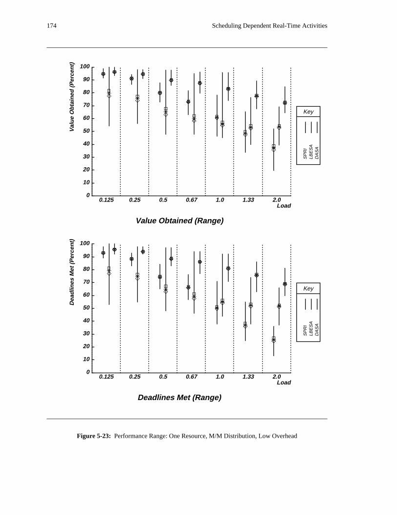
174 Scheduling Dependent Real-Time Activities
Key
SP
RI
LBE
SA
DA
SA
0
10
20
30
40
50
60
70
80
90
100V
alu
e O
bta
ined
(P
erce
nt)
Load
Value Obtained (Range)
0.125 0.25 0.5 0.67 1.0 1.33 2.0
Key
SP
RI
LBE
SA
DA
SA
0
10
20
30
40
50
60
70
80
90
100
Dea
dlin
es M
et (
Per
cen
t)
Load
Deadlines Met (Range)
0.125 0.25 0.5 0.67 1.0 1.33 2.0
Figure 5-23: Performance Range: One Resource, M/M Distribution, Low Overhead

Simulation Results 175
Key
SP
RI
LBE
SA
DA
SA
0
10
20
30
40
50
60
70
80
90
100
Val
ue
Ob
tain
ed (
Per
cen
t)
Load
Value Obtained (Range)
0.125 0.25 0.5 0.67 1.0 1.33 2.0
Key
SP
RI
LBE
SA
DA
SA
0
10
20
30
40
50
60
70
80
90
100
Dea
dlin
es M
et (
Per
cen
t)
Load
Deadlines Met (Range)
0.125 0.25 0.5 0.67 1.0 1.33 2.0
Figure 5-24: Performance Range: Five Resources, M/M Distribution, Low Overhead
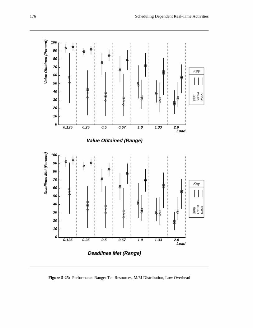
176 Scheduling Dependent Real-Time Activities
Key
SP
RI
LBE
SA
DA
SA
0
10
20
30
40
50
60
70
80
90
100V
alu
e O
bta
ined
(P
erce
nt)
Load
Value Obtained (Range)
0.125 0.25 0.5 0.67 1.0 1.33 2.0
Key
SP
RI
LBE
SA
DA
SA
0
10
20
30
40
50
60
70
80
90
100
Dea
dlin
es M
et (
Per
cen
t)
Load
Deadlines Met (Range)
0.125 0.25 0.5 0.67 1.0 1.33 2.0
Figure 5-25: Performance Range: Ten Resources, M/M Distribution, Low Overhead
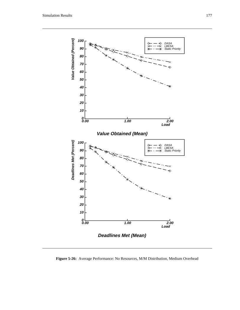
Simulation Results 177
0
10
20
30
40
50
60
70
80
90
100
Val
ue
Ob
tain
ed (
Per
cen
t)
0.00 1.00 2.00Load
Value Obtained (Mean)
Static PriorityLBESADASA
0
10
20
30
40
50
60
70
80
90
100
Dea
dlin
es M
et (
Per
cen
t)
0.00 1.00 2.00Load
Deadlines Met (Mean)
Static PriorityLBESADASA
Figure 5-26: Average Performance: No Resources, M/M Distribution, Medium Overhead
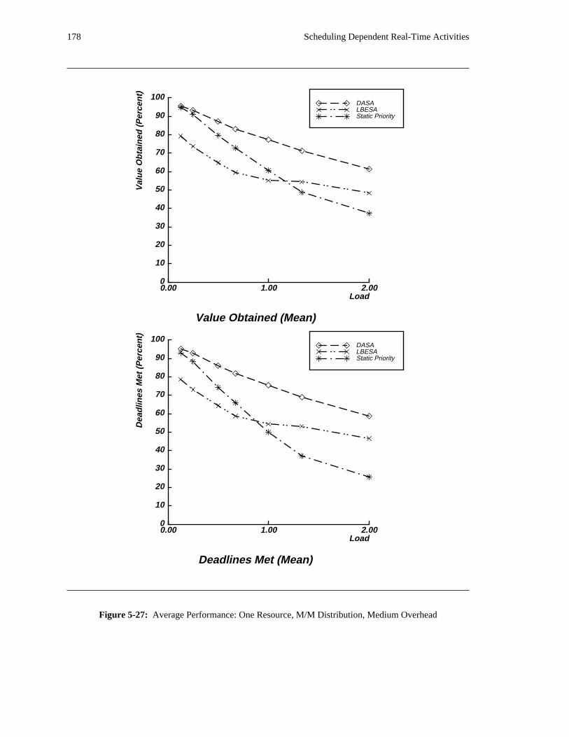
178 Scheduling Dependent Real-Time Activities
0
10
20
30
40
50
60
70
80
90
100
Val
ue
Ob
tain
ed (
Per
cen
t)
0.00 1.00 2.00Load
Value Obtained (Mean)
Static PriorityLBESADASA
0
10
20
30
40
50
60
70
80
90
100
Dea
dlin
es M
et (
Per
cen
t)
0.00 1.00 2.00Load
Deadlines Met (Mean)
Static PriorityLBESADASA
Figure 5-27: Average Performance: One Resource, M/M Distribution, Medium Overhead
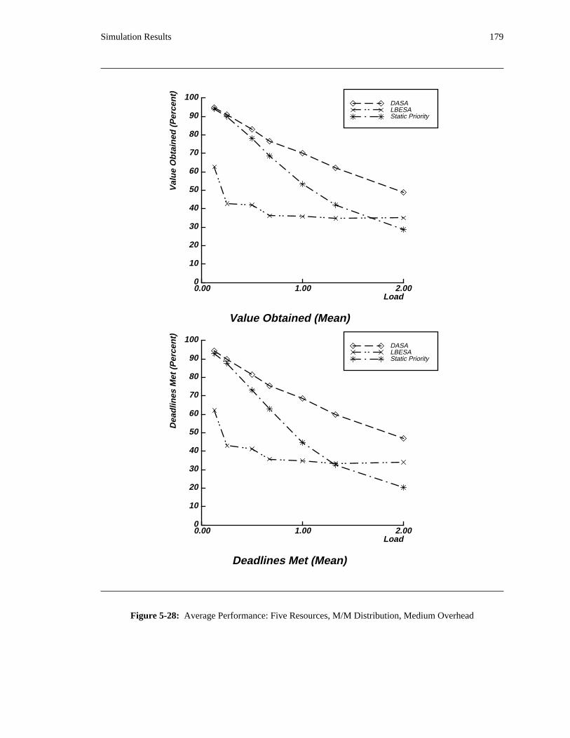
Simulation Results 179
0
10
20
30
40
50
60
70
80
90
100
Val
ue
Ob
tain
ed (
Per
cen
t)
0.00 1.00 2.00Load
Value Obtained (Mean)
Static PriorityLBESADASA
0
10
20
30
40
50
60
70
80
90
100
Dea
dlin
es M
et (
Per
cen
t)
0.00 1.00 2.00Load
Deadlines Met (Mean)
Static PriorityLBESADASA
Figure 5-28: Average Performance: Five Resources, M/M Distribution, Medium Overhead
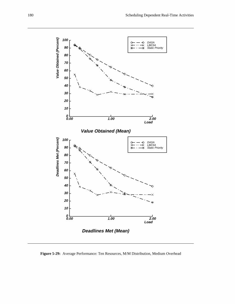
180 Scheduling Dependent Real-Time Activities
0
10
20
30
40
50
60
70
80
90
100
Val
ue
Ob
tain
ed (
Per
cen
t)
0.00 1.00 2.00Load
Value Obtained (Mean)
Static PriorityLBESADASA
0
10
20
30
40
50
60
70
80
90
100
Dea
dlin
es M
et (
Per
cen
t)
0.00 1.00 2.00Load
Deadlines Met (Mean)
Static PriorityLBESADASA
Figure 5-29: Average Performance: Ten Resources, M/M Distribution, Medium Overhead
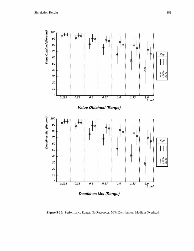
Simulation Results 181
Key
SP
RI
LBE
SA
DA
SA
0
10
20
30
40
50
60
70
80
90
100
Val
ue
Ob
tain
ed (
Per
cen
t)
Load
Value Obtained (Range)
0.125 0.25 0.5 0.67 1.0 1.33 2.0
Key
SP
RI
LBE
SA
DA
SA
0
10
20
30
40
50
60
70
80
90
100
Dea
dlin
es M
et (
Per
cen
t)
Load
Deadlines Met (Range)
0.125 0.25 0.5 0.67 1.0 1.33 2.0
Figure 5-30: Performance Range: No Resources, M/M Distribution, Medium Overhead
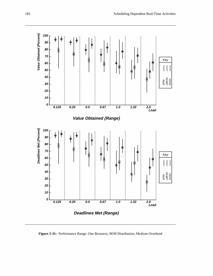
182 Scheduling Dependent Real-Time Activities
Key
SP
RI
LBE
SA
DA
SA
0
10
20
30
40
50
60
70
80
90
100V
alu
e O
bta
ined
(P
erce
nt)
Load
Value Obtained (Range)
0.125 0.25 0.5 0.67 1.0 1.33 2.0
Key
SP
RI
LBE
SA
DA
SA
0
10
20
30
40
50
60
70
80
90
100
Dea
dlin
es M
et (
Per
cen
t)
Load
Deadlines Met (Range)
0.125 0.25 0.5 0.67 1.0 1.33 2.0
Figure 5-31: Performance Range: One Resource, M/M Distribution, Medium Overhead
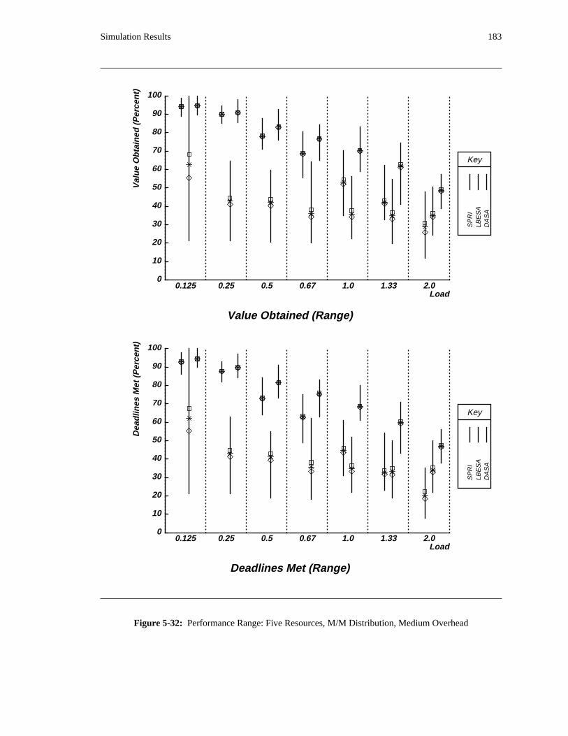
Simulation Results 183
Key
SP
RI
LBE
SA
DA
SA
0
10
20
30
40
50
60
70
80
90
100
Val
ue
Ob
tain
ed (
Per
cen
t)
Load
Value Obtained (Range)
0.125 0.25 0.5 0.67 1.0 1.33 2.0
Key
SP
RI
LBE
SA
DA
SA
0
10
20
30
40
50
60
70
80
90
100
Dea
dlin
es M
et (
Per
cen
t)
Load
Deadlines Met (Range)
0.125 0.25 0.5 0.67 1.0 1.33 2.0
Figure 5-32: Performance Range: Five Resources, M/M Distribution, Medium Overhead
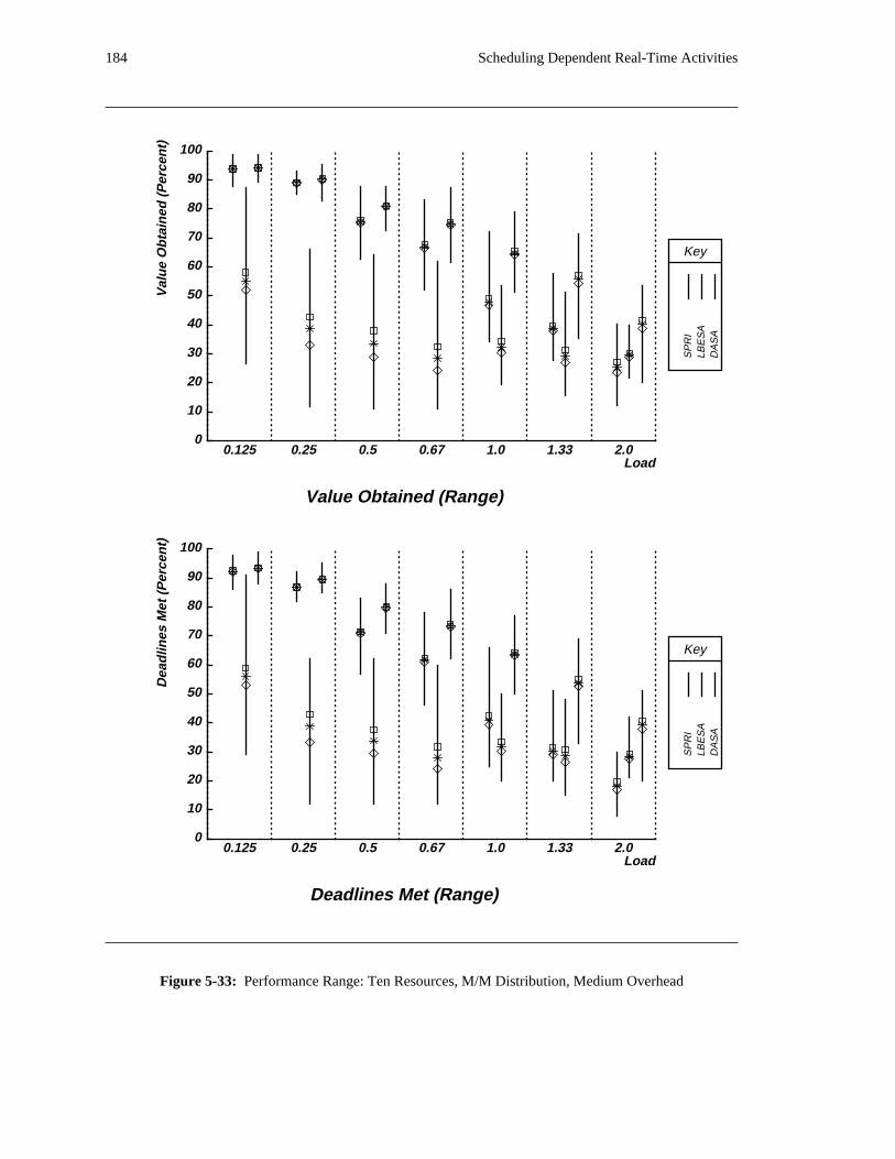
184 Scheduling Dependent Real-Time Activities
Key
SP
RI
LBE
SA
DA
SA
0
10
20
30
40
50
60
70
80
90
100V
alu
e O
bta
ined
(P
erce
nt)
Load
Value Obtained (Range)
0.125 0.25 0.5 0.67 1.0 1.33 2.0
Key
SP
RI
LBE
SA
DA
SA
0
10
20
30
40
50
60
70
80
90
100
Dea
dlin
es M
et (
Per
cen
t)
Load
Deadlines Met (Range)
0.125 0.25 0.5 0.67 1.0 1.33 2.0
Figure 5-33: Performance Range: Ten Resources, M/M Distribution, Medium Overhead
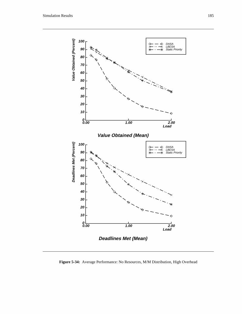
Simulation Results 185
0
10
20
30
40
50
60
70
80
90
100
Val
ue
Ob
tain
ed (
Per
cen
t)
0.00 1.00 2.00Load
Value Obtained (Mean)
Static PriorityLBESADASA
0
10
20
30
40
50
60
70
80
90
100
Dea
dlin
es M
et (
Per
cen
t)
0.00 1.00 2.00Load
Deadlines Met (Mean)
Static PriorityLBESADASA
Figure 5-34: Average Performance: No Resources, M/M Distribution, High Overhead
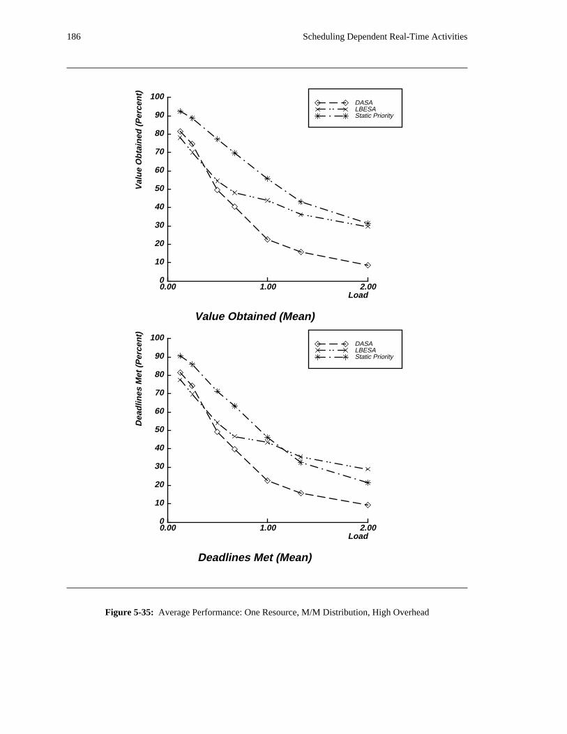
186 Scheduling Dependent Real-Time Activities
0
10
20
30
40
50
60
70
80
90
100
Val
ue
Ob
tain
ed (
Per
cen
t)
0.00 1.00 2.00Load
Value Obtained (Mean)
Static PriorityLBESADASA
0
10
20
30
40
50
60
70
80
90
100
Dea
dlin
es M
et (
Per
cen
t)
0.00 1.00 2.00Load
Deadlines Met (Mean)
Static PriorityLBESADASA
Figure 5-35: Average Performance: One Resource, M/M Distribution, High Overhead
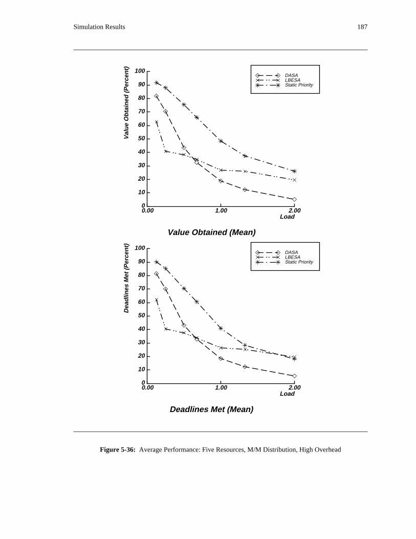
Simulation Results 187
0
10
20
30
40
50
60
70
80
90
100
Val
ue
Ob
tain
ed (
Per
cen
t)
0.00 1.00 2.00Load
Value Obtained (Mean)
Static PriorityLBESADASA
0
10
20
30
40
50
60
70
80
90
100
Dea
dlin
es M
et (
Per
cen
t)
0.00 1.00 2.00Load
Deadlines Met (Mean)
Static PriorityLBESADASA
Figure 5-36: Average Performance: Five Resources, M/M Distribution, High Overhead
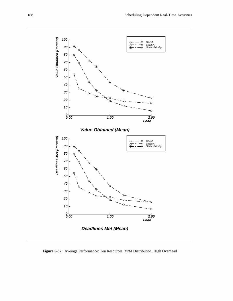
188 Scheduling Dependent Real-Time Activities
0
10
20
30
40
50
60
70
80
90
100
Val
ue
Ob
tain
ed (
Per
cen
t)
0.00 1.00 2.00Load
Value Obtained (Mean)
Static PriorityLBESADASA
0
10
20
30
40
50
60
70
80
90
100
Dea
dlin
es M
et (
Per
cen
t)
0.00 1.00 2.00Load
Deadlines Met (Mean)
Static PriorityLBESADASA
Figure 5-37: Average Performance: Ten Resources, M/M Distribution, High Overhead
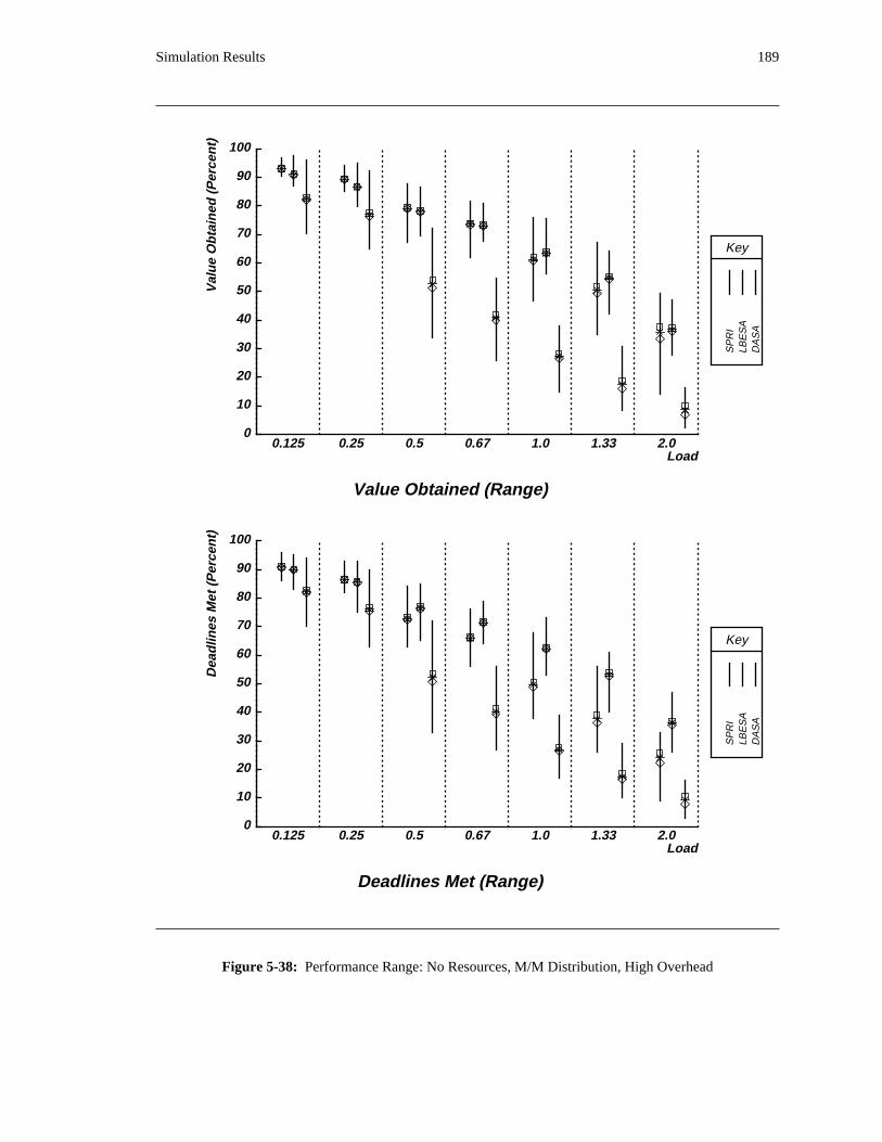
Simulation Results 189
Key
SP
RI
LBE
SA
DA
SA
0
10
20
30
40
50
60
70
80
90
100
Val
ue
Ob
tain
ed (
Per
cen
t)
Load
Value Obtained (Range)
0.125 0.25 0.5 0.67 1.0 1.33 2.0
Key
SP
RI
LBE
SA
DA
SA
0
10
20
30
40
50
60
70
80
90
100
Dea
dlin
es M
et (
Per
cen
t)
Load
Deadlines Met (Range)
0.125 0.25 0.5 0.67 1.0 1.33 2.0
Figure 5-38: Performance Range: No Resources, M/M Distribution, High Overhead
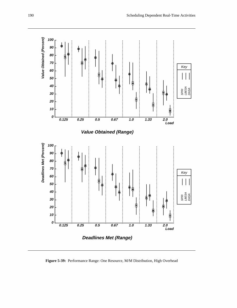
190 Scheduling Dependent Real-Time Activities
Key
SP
RI
LBE
SA
DA
SA
0
10
20
30
40
50
60
70
80
90
100V
alu
e O
bta
ined
(P
erce
nt)
Load
Value Obtained (Range)
0.125 0.25 0.5 0.67 1.0 1.33 2.0
Key
SP
RI
LBE
SA
DA
SA
0
10
20
30
40
50
60
70
80
90
100
Dea
dlin
es M
et (
Per
cen
t)
Load
Deadlines Met (Range)
0.125 0.25 0.5 0.67 1.0 1.33 2.0
Figure 5-39: Performance Range: One Resource, M/M Distribution, High Overhead
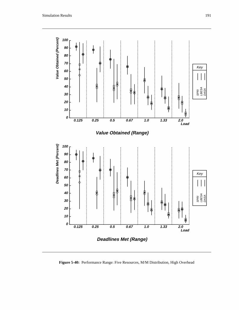
Simulation Results 191
Key
SP
RI
LBE
SA
DA
SA
0
10
20
30
40
50
60
70
80
90
100
Val
ue
Ob
tain
ed (
Per
cen
t)
Load
Value Obtained (Range)
0.125 0.25 0.5 0.67 1.0 1.33 2.0
Key
SP
RI
LBE
SA
DA
SA
0
10
20
30
40
50
60
70
80
90
100
Dea
dlin
es M
et (
Per
cen
t)
Load
Deadlines Met (Range)
0.125 0.25 0.5 0.67 1.0 1.33 2.0
Figure 5-40: Performance Range: Five Resources, M/M Distribution, High Overhead
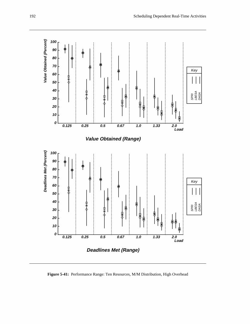
192 Scheduling Dependent Real-Time Activities
Key
SP
RI
LBE
SA
DA
SA
0
10
20
30
40
50
60
70
80
90
100V
alu
e O
bta
ined
(P
erce
nt)
Load
Value Obtained (Range)
0.125 0.25 0.5 0.67 1.0 1.33 2.0
Key
SP
RI
LBE
SA
DA
SA
0
10
20
30
40
50
60
70
80
90
100
Dea
dlin
es M
et (
Per
cen
t)
Load
Deadlines Met (Range)
0.125 0.25 0.5 0.67 1.0 1.33 2.0
Figure 5-41: Performance Range: Ten Resources, M/M Distribution, High Overhead
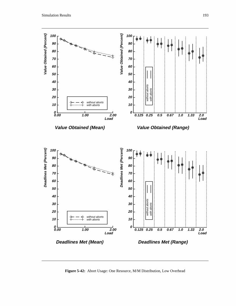
Simulation Results 193
0
10
20
30
40
50
60
70
80
90
100
Val
ue
Ob
tain
ed (
Per
cen
t)
0.00 1.00 2.00Load
Value Obtained (Mean)
with abortswithout aborts
0
10
20
30
40
50
60
70
80
90
100
Val
ue
Ob
tain
ed (
Per
cen
t)Load
Value Obtained (Range)
0.125 0.25 0.5 0.67 1.0 1.33 2.0
with
out a
bort
sw
ith a
bort
s
0
10
20
30
40
50
60
70
80
90
100
Dea
dlin
es M
et (
Per
cen
t)
0.00 1.00 2.00Load
Deadlines Met (Mean)
with abortswithout aborts
0
10
20
30
40
50
60
70
80
90
100
Dea
dlin
es M
et (
Per
cen
t)
Load
Deadlines Met (Range)
0.125 0.25 0.5 0.67 1.0 1.33 2.0
with
out a
bort
sw
ith a
bort
s
Figure 5-42: Abort Usage: One Resource, M/M Distribution, Low Overhead

194 Scheduling Dependent Real-Time Activities
0
10
20
30
40
50
60
70
80
90
100V
alu
e O
bta
ined
(P
erce
nt)
0.00 1.00 2.00Load
Value Obtained (Mean)
with abortswithout aborts
0
10
20
30
40
50
60
70
80
90
100
Val
ue
Ob
tain
ed (
Per
cen
t)
Load
Value Obtained (Range)
0.125 0.25 0.5 0.67 1.0 1.33 2.0
with
out a
bort
sw
ith a
bort
s
0
10
20
30
40
50
60
70
80
90
100
Dea
dlin
es M
et (
Per
cen
t)
0.00 1.00 2.00Load
Deadlines Met (Mean)
with abortswithout aborts
0
10
20
30
40
50
60
70
80
90
100
Dea
dlin
es M
et (
Per
cen
t)
Load
Deadlines Met (Range)
0.125 0.25 0.5 0.67 1.0 1.33 2.0
with
out a
bort
sw
ith a
bort
s
Figure 5-43: Abort Usage: One Resource, M/M Distribution, Medium Overhead
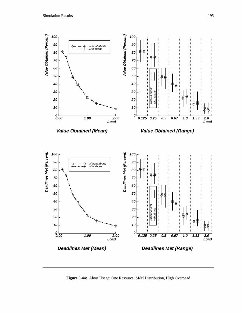
Simulation Results 195
0
10
20
30
40
50
60
70
80
90
100
Val
ue
Ob
tain
ed (
Per
cen
t)
0.00 1.00 2.00Load
Value Obtained (Mean)
with abortswithout aborts
0
10
20
30
40
50
60
70
80
90
100
Val
ue
Ob
tain
ed (
Per
cen
t)Load
Value Obtained (Range)
0.125 0.25 0.5 0.67 1.0 1.33 2.0
with
out a
bort
sw
ith a
bort
s
0
10
20
30
40
50
60
70
80
90
100
Dea
dlin
es M
et (
Per
cen
t)
0.00 1.00 2.00Load
Deadlines Met (Mean)
with abortswithout aborts
0
10
20
30
40
50
60
70
80
90
100
Dea
dlin
es M
et (
Per
cen
t)
Load
Deadlines Met (Range)
0.125 0.25 0.5 0.67 1.0 1.33 2.0
with
out a
bort
sw
ith a
bort
s
Figure 5-44: Abort Usage: One Resource, M/M Distribution, High Overhead
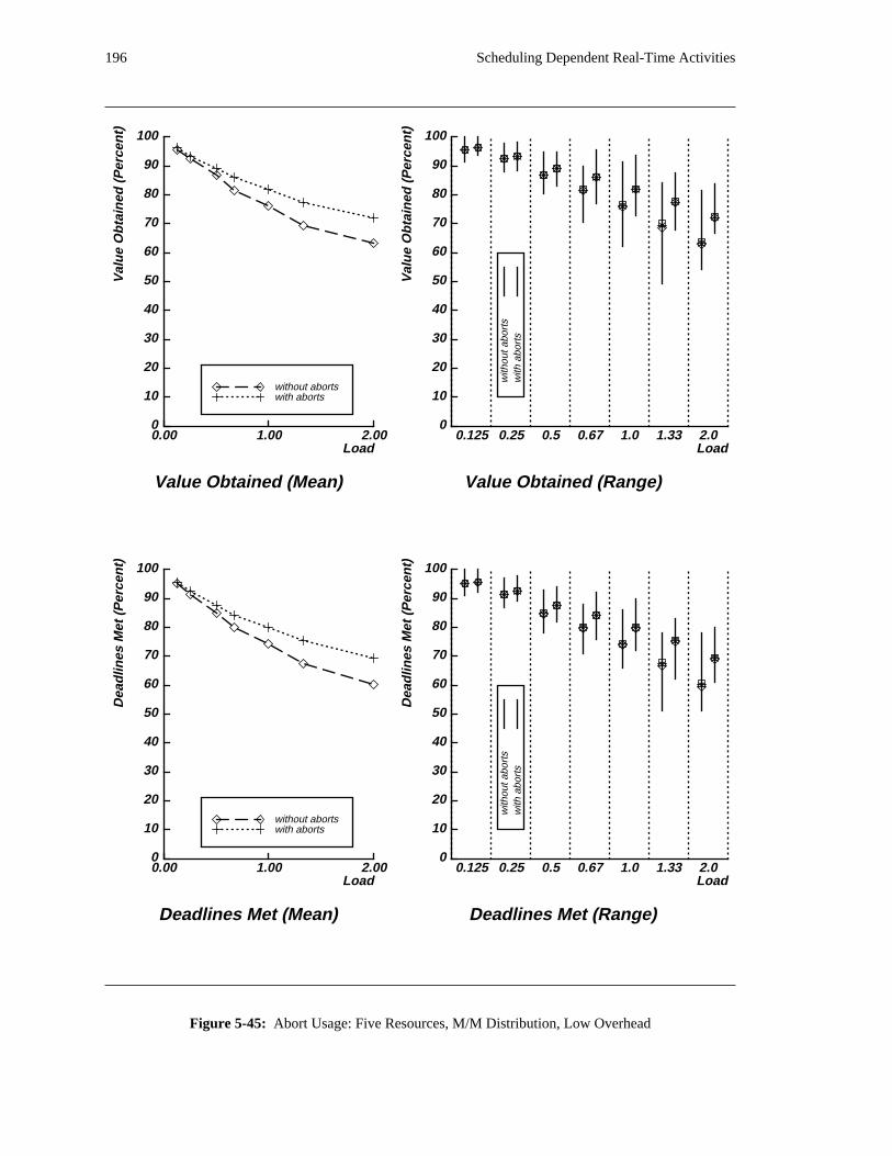
196 Scheduling Dependent Real-Time Activities
0
10
20
30
40
50
60
70
80
90
100V
alu
e O
bta
ined
(P
erce
nt)
0.00 1.00 2.00Load
Value Obtained (Mean)
with abortswithout aborts
0
10
20
30
40
50
60
70
80
90
100
Val
ue
Ob
tain
ed (
Per
cen
t)
Load
Value Obtained (Range)
0.125 0.25 0.5 0.67 1.0 1.33 2.0
with
out a
bort
sw
ith a
bort
s
0
10
20
30
40
50
60
70
80
90
100
Dea
dlin
es M
et (
Per
cen
t)
0.00 1.00 2.00Load
Deadlines Met (Mean)
with abortswithout aborts
0
10
20
30
40
50
60
70
80
90
100
Dea
dlin
es M
et (
Per
cen
t)
Load
Deadlines Met (Range)
0.125 0.25 0.5 0.67 1.0 1.33 2.0
with
out a
bort
sw
ith a
bort
s
Figure 5-45: Abort Usage: Five Resources, M/M Distribution, Low Overhead
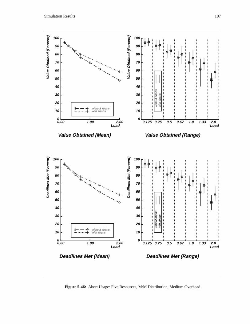
Simulation Results 197
0
10
20
30
40
50
60
70
80
90
100
Val
ue
Ob
tain
ed (
Per
cen
t)
0.00 1.00 2.00Load
Value Obtained (Mean)
with abortswithout aborts
0
10
20
30
40
50
60
70
80
90
100
Val
ue
Ob
tain
ed (
Per
cen
t)Load
Value Obtained (Range)
0.125 0.25 0.5 0.67 1.0 1.33 2.0
with
out a
bort
sw
ith a
bort
s
0
10
20
30
40
50
60
70
80
90
100
Dea
dlin
es M
et (
Per
cen
t)
0.00 1.00 2.00Load
Deadlines Met (Mean)
with abortswithout aborts
0
10
20
30
40
50
60
70
80
90
100
Dea
dlin
es M
et (
Per
cen
t)
Load
Deadlines Met (Range)
0.125 0.25 0.5 0.67 1.0 1.33 2.0
with
out a
bort
sw
ith a
bort
s
Figure 5-46: Abort Usage: Five Resources, M/M Distribution, Medium Overhead
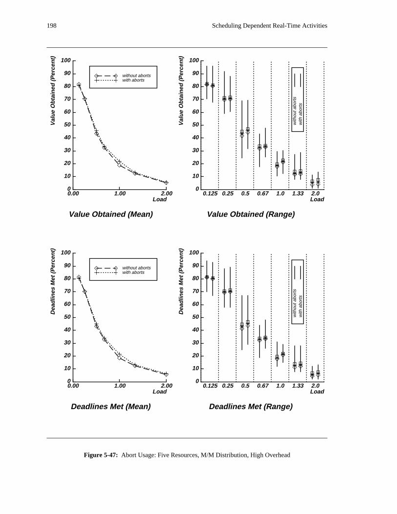
198 Scheduling Dependent Real-Time Activities
0
10
20
30
40
50
60
70
80
90
100V
alu
e O
bta
ined
(P
erce
nt)
0.00 1.00 2.00Load
Value Obtained (Mean)
with abortswithout aborts
0
10
20
30
40
50
60
70
80
90
100
Val
ue
Ob
tain
ed (
Per
cen
t)
Load
Value Obtained (Range)
0.125 0.25 0.5 0.67 1.0 1.33 2.0
with
out a
bort
sw
ith a
bort
s
0
10
20
30
40
50
60
70
80
90
100
Dea
dlin
es M
et (
Per
cen
t)
0.00 1.00 2.00Load
Deadlines Met (Mean)
with abortswithout aborts
0
10
20
30
40
50
60
70
80
90
100
Dea
dlin
es M
et (
Per
cen
t)
Load
Deadlines Met (Range)
0.125 0.25 0.5 0.67 1.0 1.33 2.0
with
out a
bort
sw
ith a
bort
s
Figure 5-47: Abort Usage: Five Resources, M/M Distribution, High Overhead
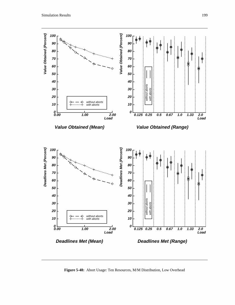
Simulation Results 199
0
10
20
30
40
50
60
70
80
90
100
Val
ue
Ob
tain
ed (
Per
cen
t)
0.00 1.00 2.00Load
Value Obtained (Mean)
with abortswithout aborts
0
10
20
30
40
50
60
70
80
90
100
Val
ue
Ob
tain
ed (
Per
cen
t)Load
Value Obtained (Range)
0.125 0.25 0.5 0.67 1.0 1.33 2.0
with
out a
bort
sw
ith a
bort
s
0
10
20
30
40
50
60
70
80
90
100
Dea
dlin
es M
et (
Per
cen
t)
0.00 1.00 2.00Load
Deadlines Met (Mean)
with abortswithout aborts
0
10
20
30
40
50
60
70
80
90
100
Dea
dlin
es M
et (
Per
cen
t)
Load
Deadlines Met (Range)
0.125 0.25 0.5 0.67 1.0 1.33 2.0
with
out a
bort
sw
ith a
bort
s
Figure 5-48: Abort Usage: Ten Resources, M/M Distribution, Low Overhead
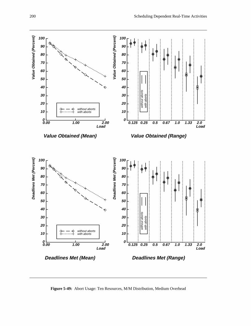
200 Scheduling Dependent Real-Time Activities
0
10
20
30
40
50
60
70
80
90
100V
alu
e O
bta
ined
(P
erce
nt)
0.00 1.00 2.00Load
Value Obtained (Mean)
with abortswithout aborts
0
10
20
30
40
50
60
70
80
90
100
Val
ue
Ob
tain
ed (
Per
cen
t)
Load
Value Obtained (Range)
0.125 0.25 0.5 0.67 1.0 1.33 2.0
with
out a
bort
sw
ith a
bort
s
0
10
20
30
40
50
60
70
80
90
100
Dea
dlin
es M
et (
Per
cen
t)
0.00 1.00 2.00Load
Deadlines Met (Mean)
with abortswithout aborts
0
10
20
30
40
50
60
70
80
90
100
Dea
dlin
es M
et (
Per
cen
t)
Load
Deadlines Met (Range)
0.125 0.25 0.5 0.67 1.0 1.33 2.0
with
out a
bort
sw
ith a
bort
s
Figure 5-49: Abort Usage: Ten Resources, M/M Distribution, Medium Overhead
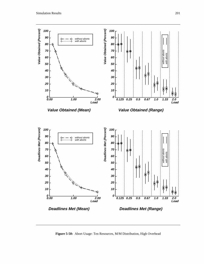
Simulation Results 201
0
10
20
30
40
50
60
70
80
90
100
Val
ue
Ob
tain
ed (
Per
cen
t)
0.00 1.00 2.00Load
Value Obtained (Mean)
with abortswithout aborts
0
10
20
30
40
50
60
70
80
90
100
Val
ue
Ob
tain
ed (
Per
cen
t)Load
Value Obtained (Range)
0.125 0.25 0.5 0.67 1.0 1.33 2.0
with
out a
bort
sw
ith a
bort
s
0
10
20
30
40
50
60
70
80
90
100
Dea
dlin
es M
et (
Per
cen
t)
0.00 1.00 2.00Load
Deadlines Met (Mean)
with abortswithout aborts
0
10
20
30
40
50
60
70
80
90
100
Dea
dlin
es M
et (
Per
cen
t)
Load
Deadlines Met (Range)
0.125 0.25 0.5 0.67 1.0 1.33 2.0
with
out a
bort
sw
ith a
bort
s
Figure 5-50: Abort Usage: Ten Resources, M/M Distribution, High Overhead

202 Scheduling Dependent Real-Time Activities
Chapter 6
Related Work and Current Practice
There has been a great deal of research done on scheduling algorithms, in general, and scheduling
algorithms for real-time systems, in particular, through the years. This chapter explains where this thesis
research belongs within this overall context.
Most of the basic scheduling algorithms are covered in text books on scheduling [Baker 74, French 82] or
on operating systems [Janson 85, Peterson 85]. Each algorithm possesses certain properties that
differentiate it from others. For instance, round-robin is fair, while shortest processing time first maximizes
throughput. While many of these properties have no intrinsic value in real-time systems, these texts also
contain some scheduling algorithms that are useful in real-time systems.
Real-time systems can be large and complex, possibly comprising several processors that embody a
hierarchically-structured system. Each level of the system may be characterized by different requirements
and capabilities. For instance, at the lowest level, programmable controllers may periodically monitor
sensors and adjust actuators to maintain desired set points for physical processes, while at the next higher
level, supervisory control computers coordinate the actions of the programmable controllers, handle
exception conditions, and attempt to satisfy higher-level goals. In the case of programmable controllers,
the workload is regular −− it occurs at specific intervals and involves fixed computations on known sets of
data. For supervisory control systems, the workload is more dynamic −− exceptions occur irregularly and
the programmable controllers operate asynchronously with respect to one another, but stringent response
time requirements may still be placed on its actions. Higher level systems typically operate under fewer,59less restrictive time constraints and handle long-range planning and monitoring functions .
The differing real-time requirements and workload characteristics of these hierarchical levels suggest that
different scheduling methods may be appropriate for each level. For instance, simple list schedulers may
be well-suited for the lowest system levels; schedulers capable of handling more dynamic real-time loads,
such as DASA, may be most appropriate for the supervisory control level; and the strategic scheduling
performed at the highest system levels may employ large, complex models like those used in operations
research. Unfortunately, the literature often refers to "real-time systems" or "real-time scheduling
algorithms" without explicitly specifying which level in the real-time system hierarchy is being addressed.
59Of course, the meaning of "long-range" is determined by the nature of the application. It might mean anything from minutes tohours, or even longer.
203
204 Scheduling Dependent Real-Time Activities
The following discussion examines a number of real-time scheduling algorithms and describes their
applicability within the real-time system hierarchy outlined above. Particular attention is paid to the use of
algorithms for supervisory control scheduling.
Real-time scheduling algorithms can be categorized in a number of ways. For the following discussion,
they are divided into three groups: priority-based, deadline-based, and time-driven. Briefly, priority-based
algorithms make scheduling decisions according to a single value that is assigned to each activity in the
system. This value generally indicates the overall functional importance of the activity to the application.
Deadline-based algorithms also make scheduling decisions based on a single value. In this case, the value
is the activity’s deadline, which indicates the urgency of the activity. Time-driven algorithms consider both
the functional importance and the urgency of each activity when making scheduling decisions.
The discussion of these three groups of scheduling algorithms is followed by a section devoted to other
algorithms that are of interest in establishing the context for this research, but are not properly part of these
three groups.
6.1. Priority-Based Scheduling
Most of the real-time systems currently in service employ a static priority scheduler of one type or
another. In these systems, component activities are assigned static priorities, and the systems are tuned so
that they will typically meet their time constraints. There is also a large body of literature that has
investigated priority-based scheduling algorithms beyond this current practice. In [Liu 73], a method for
static priority assignment was presented for periodic real-time activities. The scheduling discipline that has
grown from this work is called rate monotonic scheduling. This basic approach has been elaborated and
expanded upon since (see for instance [Sha 86] and [Sha 90]), but the applications for which it is intended
are always those where most, if not all, of the activities are periodic, and where the periodic activities are
nearly always the most important activities in the system. While there are systems that fit this description,
the family of supervisory control systems that are of interest in this thesis do not.
A second class of priority-based scheduling algorithms has dealt explicitly with some of the scheduling
difficulties that arise as a result of the dynamic interaction of activities. Some operating systems (for
example, VMS [KB 84]) implement priority adjustment schemes to refine the simple static priority model,
and other schemes have been proposed in the literature as well ( [Sha 87]). [Rajkumar 89] addresses the
synchronization of periodic activities within a rate monotonic framework, attempting to put upper bounds
on the length of time that a lower priority activity may block a higher priority activity as a consequence of a
resource conflict. All of these schemes address problems in which a lower priority activity that shares a
resource with a higher priority activity can block the higher priority activity for an arbitrarily long time.
The solution, roughly speaking, allows the lower priority activity to assume a higher priority for at least
long enough to complete its access to the shared resource, thereby allowing the higher priority activity to
resume. This approach does solve some problems that are associated with simple priority-based scheduling
algorithms, but it does not come to grips with the fundamental shortcoming of all of the priority-based
schemes: priorities are unable to adequately capture the critical scheduling information for activities.
Related Work and Current Practice 205
Specifically, an individual activity’s importance to the overall application and its urgency are two
independent factors: an activity is not urgent just because it is very important, and it is not important just
because it is urgent. This distinction is lost in static priority scheduling schemes where both importance
and urgency must be reflected in a single quantity, the activity’s priority.
6.2. Deadline-Based and Time-Driven Scheduling
This section discusses both deadline-based and time-driven scheduling since they both use time as a
primary criterion for making scheduling decisions, and since time-driven scheduling algorithms evolve60naturally from deadline-based scheduling algorithms .
Deadline-based and time-driven algorithms seem well-suited for use in real-time systems since they
explicitly take into account activities’ time constraints, and they do not typically require that all activities
be periodic. Deadline schedulers have been in use in operating systems at least since the 1960s, and [Liu
73] demonstrated the optimality of deadline scheduling under one computational model. Unfortunately, the
basic deadline scheduling algorithm becomes unstable whenever an overload occurs; it acts to minimize the
maximum job lateness and maximum job tardiness( [Conway 67]). This may be the desired action, but
often it is not. Consequently, a great deal of work has been done to modify the behavior of deadline
scheduling in overload situations. Some work that does not consider dependency requirements includes:
[Martel 82], which presents an algorithm that will complete all of the (independent) activities while
minimizing the maximum lateness of any individual activity; [Moore 68], which uses a scheme that also
completes all of the independent activities while minimizing the maximum deferral cost associated with
any activity; and [Locke 86], which does not necessarily execute all of the activities, but does attempt to
maximize the value acquired by completing those that are executed. In each case, these schemes do not
consider dependencies, but do address the issue of overload handling, which is one of the main interests of
this thesis.
Historically, there has been a great deal of emphasis placed on being able to guarantee that deadlines can
be met. In simple systems that have been built, this has been possible, or has at least appeared to be
possible. As systems have grown, this has become increasingly more difficult to do. In large, dynamic
systems, it is rapidly becoming impossible. Nonetheless, guaranteeing that deadlines can be met is often
considered a prime requirement for so called hard real-time systems, and much work has been done in this
area. (In a hard real-time system, missing even a single deadline means that the entire system has failed.)
For simple systems where all of the activities need to be scheduled periodically and have fixed execution
time requirements, [Liu 73] and others allow an off-line analysis to guarantee the schedulability of a set of
activities under certain assumptions. In more dynamic cases where less emphasis is placed on periodic
activities, work similar to [Ramamritham 84] attempts to provide the same type of guarantee. However, it
is not obvious that attempting to offer true guarantees is wise in a dynamic system because honoring a
guarantee may result in an inability to schedule a new activity that is clearly more important and more
60In some of the management and operations research literature, deadlines are referred to as due dates.
206 Scheduling Dependent Real-Time Activities
urgent than the previously guaranteed activity. In addition, the guarantees that are offered are not absolute.
Receiving a guarantee indicates that adequate resources have been reserved to complete an activity by the
desired time. If resources are subsequently lost −− due to a processor or a power failure, for example −−the guarantees made cannot always be honored.
There is also a body of literature that explicitly deals with dependencies in deadline-based scheduling
algorithms. It should be noted that what is termed a dependency consideration in this thesis encompasses
both the notion of a precedence constraint (where, for instance, activity A must complete before activity A1 2
may begin) and the notion of a resource requirement (where, for example, activity A requires exclusive use1
of resource R for time T during its execution). In the literature, these two types of dependencies are often
treated separately. [Blazewicz 77], for instance, deals only with precedence constraints and provides an
algorithm that will allow activities with different arrival times and known, fixed precedence constraints to
be scheduled in a hard real-time system. This algorithm can be thought of as a deadline inheritance
algorithm, whereby an activity is scheduled as if it had a deadline "close" to that possessed by another61activity that both depends on it and has a nearer deadline. Unfortunately, these precedence constraints are
fixed, making a straightforward extension to handle resource requirements difficult. Also, no effort is
made to handle overload cases, since, by Blazewicz’s definition, a missed deadline means that the entire
system has failed.
[Cheng 86] looks only at precedence constraints, while [Zhao 87] looks at both precedence constraints
and resource requirements. In both cases, these represent extensions of [Ramamritham 84] and share the
same shortcomings −− they attempt to make guarantees to run specific activities at the possible expense of
more urgent or more important activities that may arrive later, and the guarantees are not truly guarantees
since unanticipated problems can prevent their fulfillment. In addition, although [Zhao 87] presents a more
dynamic, less restrictive model than that presented in most of the work in this area, knowledge of the
specific resource requirements of any activity to be run is still assumed to be known in advance.
[Lawler 73] deals with precedence constraints when scheduling a group of activities on a single machine
and presents an algorithm that uses a monotone cost function to derive a schedule that minimizes the
maximum of the incurred costs. However, the activities to be scheduled have no deadlines, nor do they
have any resource requirements. [Elsayed 82] presents heuristics to schedule a set of activities that share
resources to complete a project. Once again, there are no deadlines associated with any of the activities.
Some of the previous references deal with uniprocessor scheduling, and some deal with multiprocessor or
multiple processor scheduling. This distinction was not made previously because the number of62processors, although certainly an important consideration , is of secondary concern for the work at hand.
61In fact, one view of the DASA algorithm to be examined in the thesis work is exactly this. It incorporates the idea that the activitieson which some activity depends must be dealt with before the activity’s deadline, as must the activity itself. However, in addition, thealgorithm assesses the situation to decide if there is currently an overload, and if so, selects the subset of activities to be run accordingto a meaningful metric.
62Note, for instance, that a scheduling algorithm that is optimal for a uniprocessor may not be optimal for a multiprocessor. Asimple deadline scheduler with no overloads demonstrates this fact.
Related Work and Current Practice 207
The primary issues being addressed when comparing and contrasting those efforts with this one are:
whether or not time constraints are dealt with explicitly, the amount and type of information on which
scheduling decisions are based, and the fundamental nature of applications (whether they are static or
dynamic, periodic or aperiodic; whether overloads can occur and if so how they are handled). And,
although a great deal of work has touched on various aspects of the thesis problem, none of this work has
addressed all of the key issues at once.
6.3. Other Related Work
The computational model presented in this thesis provides for the abortion of an activity. This is done for
two reasons. First of all, in any application, if an activity that manipulates shared resources is to be
terminated, unless specific steps are taken there is a danger that the shared resources will either be
unavailable for use by other activities or left in an inconsistent state. The abort mechanism addresses this
problem by allowing the shared resources to be returned to an acceptable state for later use. Secondly, an
abort mechanism similar to that just mentioned can be used to support an atomic transaction63facility [Eswaran 76]. The ability to include such a powerful facility in real-time systems is inviting , and
the work presented here can assist in making this feasible at some point.
Some work has already been done to provide atomic transactions in real-time systems. Often, this has
involved changing the concurrency control features found in traditional database transaction managers
( [Liskov 83, McKendry 85, Sha 85]). Other work has examined the problem of scheduling transactions
using the standard concurrency control rules. However, some of the models chosen for work in this area
( [Liu 88], for example) require detailed prior knowledge of the precise resource requirements and exact
access and release timings for each resource in each transaction.
A few researchers have addressed a more dynamic model, similar to that employed in this thesis.
[Stankovic 88] presents a set of rules that control access to shared data by concurrent transactions.
However, these rules are not tied to the scheduling algorithm for the processor, and they only determine
which of two competing transactions should be allowed to execute −− they do not consider a more global
view of scheduling that involves all of the transactions, perhaps involving feasibility testing of the
anticipated schedule. The scheduling rules assign a value to each competing transaction based on various
weighted factors such as time remaining until deadline, functional criticality, computation time expended
on the transaction, and so forth. Different choices of weighting factors will result in different behaviors,
but there is little analysis in this paper to aid in the selection of these factors.
[Abbott 87] discusses various scheduling algorithms that may be used for real-time transactions,
including Locke’s Best Effort scheduling algorithm. It does not discuss concurrency control rules that are
separate from the scheduling algorithm that is used to assign the processor to transactions. [Abbott
89] continues this work but does not use time-value functions or Locke’s algorithm when comparing
63In fact, [Jensen 76b] suggests using transactions not only for real-time applications, but also within a decentralized operatingsystem that supports these applications.
208 Scheduling Dependent Real-Time Activities
scheduling algorithms and concurrency control rules. In case of overload, the stated goal of the system is
to minimize the number of missed deadlines.
[HiPAC 88] reports on a project where database system researchers explore approaches to resolve
time-constrained data management problems. Their approach models transactions and the situations that
trigger their execution in order to provide efficient triggering mechanisms. Time-value functions and
time-driven scheduling constitute one of the approaches for scheduling activities that they propose to
explore and perhaps modify.
Finally, a few other research directions should be mentioned to put this work in its proper context. An
underlying assumption of this work is that dependencies among component activities are a natural product
of complex, dynamic real-time systems. There is some work that attempts to approach the construction of
applications from other points of view. [Herlihy 88] explores an approach that would eliminate the need for
any activity to wait on other activities when accessing resources. However, this approach does not allow
the maintenance of mutually consistent resources, which is often important in real-time systems. [Birman
88, Joseph 88] outline portions of a scheme that allows application-specific consistency constraints to be
satisfied by utilizing a set of communication and replication mechanisms. How to specify the behavior of
objects that have been composed in this way so that large applications can be constructed using a modular
design methodology is an important open question with respect to this approach.
Chapter 7
Future Work
The preceding chapters have demonstrated that the DASA algorithm, operating under the specified
assumptions, can benefit supervisory control applications. This chapter discusses some of the directions
that further work in the future may take −− to adapt DASA for use in real-time operating systems, to study
its performance for various applications, and to expand the domain in which it may be employed.
7.1. Loosening Assumptions
The model within which DASA was formulated embodied a set of fundamental assumptions. These
assumptions, discussed in Chapters 1 and 2, were made to reduce supervisory control scheduling to a
tractable research problem focused on a few key issues.
While these assumptions seem valid for a significant number of real-time supervisory control
applications, they may not hold for some other interesting applications. Each of the following sections
addresses one possible assumption that could be explored in the future. In each case, DASA could almost
certainly be applied to more applications if the specified assumption could be removed or loosened.
7.1.1. Known Computation Time for Phase
It has been assumed for the purposes of this research that, at the start of a given computational phase for
an activity, the amount of processor execution time that will be required to complete that phase is
accurately known. While this is not a particularly unreasonable assumption for many real-time systems, it
would be desirable to investigate the effect on the scheduler’s effectiveness if the required computation
time were not known accurately.
In some real-time systems, especially low-level control systems, the required computation time is known
precisely. The code has been written so that there is little or no variability in execution time from one
execution to the next, and the relevant code and data are always in memory when they are needed.
In other systems, it seems plausible that the operating system could be instrumented to measure the
amount of time required to execute each computational phase. As the application runs, the operating
system could form a fairly accurate profile of the required computation time for each phase. This
information could then be used by the scheduler as the phases initiate subsequent executions.
209
210 Scheduling Dependent Real-Time Activities
For a number of reasons, it would seem to be advantageous to loosen the constraints placed on such
implementations. For instance, if the required computation time can vary significantly depending on the
values of specific data items, then supplying a single estimate as the required computation time to the
scheduler will necessarily be wrong some, if not all, of the time.
Or, in a large supervisory control system, it may be impossible to guarantee that all of the application
code and data that may be needed can be memory-resident. Instead, some of it may reside in secondary
storage until it is needed. The time required to transfer the necessary code and data into main memory will
affect the required computation time, assuming the time required to access and load the information is
"charged" to the computational phase requesting it. These paging effects could make an otherwise fixed
required computation time highly variable.
The existing simulator could be used to study the sensitivity of the DASA scheduling algorithm to the
accuracy of required run-time estimates. The workloads that were previously used, as well as any new
workloads, could be modified to (intentionally) supply the scheduler with arbitrarily inaccurate
information. The same metrics that have been used in this research would be appropriate to measure the64effects of this loss of accurate information .
7.1.2. Exclusive Access to Shared Resources
All activities access shared resources in a mutually exclusive manner in the research presented in this
document.
For some shared resources, this is fine. For example, signals between pairs of activities are held by the
signaler until it is time to send the signal. Then the shared resource is released, allowing the signal receiver
to access the resource, and, hence, receive the signal. No richer set of access modes is required for such an
application.
Similarly, serialized access to a device, which may be gained by possessing an associated shared
resource, seems to be adequately addressed by mutually exclusive semantics for the acquisition and
possession of the shared resource.
Nonetheless, there are many situations where a richer set of access modes for shared resources would be
desirable. Although a signal from one phase to a set of other phases could be implemented by a set of
shared resources, each coordinating the signal sender with one signal recipient, this seems to be inefficient
and it requires the signal sender to know how many recipients there are (or may be). The ability to have all
of the recipients gain concurrent access to the shared resource once the signaler has released it would
provide a better facility to address this application need.
64Locke performed a sensitivity analysis of this sort in his thesis( [Locke 86]) and found that his algorithm was not strongly affectedby poor required computation time estimates. A similar result might hold for DASA.
Future Work 211
Certainly, in the case of shared data, a richer set of access modes would be advantageous. Concurrent
access to shared data and, to a lesser extent, shared devices is provided in many systems. When users
request access to a shared resource, they specify an access mode to the resource manager. When the
request can be satisfied without conflicting with any other outstanding resource accesses, it is granted. (See
[Date 86] for a discussion of this topic.) Since DASA subsumes the functions of the resource manager, then
it must be able to handle multiple access modes.
Adapting DASA to embody a more complex set of access modes to shared resources should be fairly
straightforward. Perhaps the most interesting design questions will arise when weighing the −− potentially
complex −− access requirements of various phases in light of the ability of the scheduler to issue aborts.
Consequently, the number of tentative schedules that may be considered when selecting a phase to execute
may increase, relative to the number considered when there is only a single access mode for shared
resources. For instance, when resources are accessed in a mutually exclusive manner, it is only necessary
to abort or complete a single phase to free a resource for use by another phase. When it is possible for
multiple phases to concurrently access a resource with possibly different access modes, then it may be
necessary to abort or complete several phases to free a single resource. Furthermore, it may be necessary to
complete or abort a (somewhat) different set of phases to free the same resource for another phase that
happens to be requesting a different access mode.
Advanced facilities to serve applications provide another reason to explore the use of a richer set of
access modes. This research is intended, in part, to lay a foundation upon which a real-time atomic
transaction facility can be built. Such a facility will demand a richer set of access modes similar to those
provided by non-real-time transaction facilities ( [Date 86]), including at least a concurrent read access
mode.
7.1.3. Simple Time-Value Functions
This research focused on phases characterized by simple time-value functions. In fact, all of the time-
value functions were step functions.
Jensen proposed a much wider range of time-value functions ( [Jensen 75]), and others have explored this
concept ( [Locke 86, Northcutt 87]). DASA could be modified to handle a wider range of functions. The
motivation for this change should come from the applications to be supported by DASA. If they need more
complex functions to describe their time constraints and values, then DASA must provide them.
65[Locke 86] used five parameters to describe a time-value function and was given the mean and
standard deviation of the expected computation time for the phase. Numerical integrations were then
performed to determine the expected value that each phase could add to the schedule being constructed. In
theory, these same extensions can be made to DASA. However, in practice, this may well be too time-
consuming.
65There were two of these time-value function 5-tuples for each phase to be scheduled: one specified the phase’s value before acritical time, and the other specified its value after that time.
212 Scheduling Dependent Real-Time Activities
The adaptation of Locke’s work that was incorporated in Release 1.0 of the Alpha Operating System
( [Northcutt 87]) used time-value functions that were described as a sequence of piecewise linear segments.
These segments could easily be integrated to yield approximate results of sufficient accuracy.
Formalizing this piecewise linear approximation in the context of DASA might be the most promising
direction to explore in order to enrich the set of time-value functions that an application may specify.
7.2. Generalizing the Model
The previous section described work that could be done if some of the assumptions that were made for
this research were changed. This section deals with similar considerations. However, rather than loosening
restrictions that were made within the model outlined in Chapters 1 and 2, this section expands the model
itself −− allowing DASA to be utilized in other, related domains.
The following discussion focuses on functional generalizations that can be made to the model: scheduling
multiprocessors and nesting phases for example. Due to this focus, the tools that can be used to perform
these generalizations are not always mentioned explicitly. Consequently, it is appropriate to mention at the
outset that the formal model that was used to express and analyze DASA may prove useful as the basis for
any future work, as well. Certainly, an appropriately modified version of the formal model should allow
functional generalizations to be defined precisely. Later, as work progresses it will become possible to
determine if useful analytic proofs can be performed. Perhaps the behavior of new algorithms can be
compared to DASA under restricted conditions, much as DASA was compared to LBESA under restricted
conditions in this thesis. This would provide some assurance that the new algorithms behaved well under
known circumstances.
7.2.1. Multiprocessor Scheduling
DASA is a uniprocessor scheduling algorithm. Multiprocessors −− that is, multiple processors that share
primary memory −− are becoming more and more common. Unfortunately, scheduling for multiprocessors
is not the same as scheduling for uniprocessors.
It is provable that a deadline-ordered schedule is optimal for a uniprocessor, provided that there are
sufficient processor cycles to meet all of the deadlines( [Liu 73]). If this same deadline scheduler were
used in a multiprocessor system, where each processor invoked the scheduler each time it needed to make a
scheduling decision, then the resulting scheduler behavior would not necessarily be optimal ( [Baker
74, Conway 67]).
Consequently, if DASA is to be effective in scheduling multiprocessors, changes should be explored that
take into account the number of available processors when generating tentative schedules. Once again, this
will result in a larger space of tentative schedules to examine since each phase could potentially be run on
any of a number of processors.
Future Work 213
Section 5.3 showed that, under many circumstances, the scheduling overhead that results from the relative
complexity of DASA is acceptable on a uniprocessor −− that is, that even though DASA consumes
considerably more processor cycles than other algorithms, it allows the application to accrue a higher value
than the other algorithms. Nonetheless, DASA is an expensive algorithm to execute.
In this light, it is possible that an appropriately adapted DASA algorithm would benefit from executing in a
multiprocessor environment. If DASA could schedule several processors at once, its cost, relative to the
amount of application work that is executed, would be reduced.
7.2.2. Multiple Node Scheduling
Once multiprocessor scheduling has been examined (or even before it has), attention can be given to
employing DASA in a distributed environment composed of multiple nodes (uniprocessors or
multiprocessors) that do not share memory. Since many supervisory control systems are, or could be,
distributed, this is a useful topic to study.
In order to have reasonable reliability and responsiveness, each node should have a local scheduler. Of
course, at any instant, each node has only localized or approximate knowledge of the overall system state.
Acquiring system-wide agreement from all of the local schedulers in order to make scheduling decisions
based on global state information would be prohibitively expensive. Therefore, a more limited form of
coordination and information-sharing among local schedulers must be explored when extending DASA into
the distributed domain.
If computational phases may span nodes, the situation is further complicated. In that case, the processing
requirements of a given phase must be satisfied by two or more nodes and scheduled by two or more
schedulers. More information will probably have to be passed to the scheduler in order to adequately
define the processor requirements for each processor that is involved with the phase. [Maynard 91] is
examining these issues in the same general context in which this research was performed, although not
specifically for DASA.
7.2.3. Grouped Resource Requests
Resources are requested and granted individually according to the model adopted for this thesis research.
This convention was adopted because it covers the most conservative case: the number and identities of the
shared resources that are required for a phase need not be known in advance.
The ability to request access to multiple resources by issuing a single request to the scheduler might
permit the scheduler to better meet the needs of the application. Currently, even if it was known that a
phase required a given set of resources to complete successfully, it could not effectively communicate this
information to the scheduler. Instead, the phase would have to request the resources one at a time, never
able to indicate that other requests would follow.
214 Scheduling Dependent Real-Time Activities
If the scheduler could anticipate the future resource requirements of a phase it could avoid certain pitfalls.
For instance, suppose a phase needed two resources, both of which are already allocated to other phases,
and, no matter which is requested first, the scheduler will determine that there is sufficient time to acquire
the resource from the phase currently holding it and still let the requesting phase complete. Then when the
first resource is requested, the scheduler will arrange to free it, allocate it to the requesting phase, and allow
that phase to execute until it requests the second resource. At that point it may determine that there is not
enough time to free that resource and allow the requesting phase to complete. Therefore, the scheduler will
not attempt to satisfy the request for the second resource. Consequently, not only were the processor cycles
that were consumed by the requesting phase wasted, but more cycles will be wasted when the phase must
be aborted to release the first resource it requested.
If the scheduler knew that the phase needed both resources in the first place, then it may have been
possible to recognize immediately that the phase could never free both resources in time to meet its
deadline. In that case, it would not have been scheduled and the processor cycles that it might otherwise
have consumed would be available for other phases.
This example demonstrates how some additional knowledge about the phase’s needs could be applied in a
straightforward manner to allocate the processor’s cycles more effectively than DASA can. Using this
additional information would, once again, increase the complexity of the scheduling algorithm. In this
case, a phase may depend on several other phases, rather than on a single phase. Determining a tentative
schedule that satisfies all of these dependencies would be more complex than it is using DASA.
Additional work would need to be done to characterize the circumstances under which the application of
this additional knowledge would benefit the application.
7.2.4. Release of Shared Resources
The model of application activities specified for this research defined each activity to be composed of a
sequence of computational phases. During each phase, shared resources may be acquired. At the
conclusion of each phase, these resources are released.
This model of resource acquisition and release fits some applications quite well, including the
conventional structure that is employed by atomic transaction facilities.
However, not all applications may follow such stylized conventions for the release of shared resources.
For example, a phase might finish with a resource before it has completed all of its work. In order to allow
another phase to acquire the resource, potentially increasing concurrency for the application, the phase66might release the resource as soon as possible .
66If this were done, the author of the phase must realize that the phase could still be aborted prior to its successful completion. Ifthe phase would need the shared resource in order to properly abort, then it would almost certainly be a mistake to release it prior tothe completion of the phase. However, if the phase would not need access to that shared resource in order to abort, then releasing theresource early may well be advantageous.
Future Work 215
On the other hand, an activity might wish to hold a shared resource past the completion of a phase. This
seems possible since, in the model employed here, phases correspond to time constraints that are typically
imposed by the external world. Certain tasks must be accomplished while satisfying those time constraints,
and shared resources may be acquired to complete those tasks. However, there seems to be no inherent
requirement that a task cannot require the use of a resource while having to satisfy two or more sequential
time constraints, which correspond to two or more computational phases.
In the future, exploring the issues that arise from decoupling the acquisition and release of resources from
the imposition of individual time constraints might be address the needs of a broader group of applications.
7.2.5. Nested Phases
This thesis has defined activities to be composed of a sequence of computational phases. It has not dealt
with the possibility of nesting phases.
Nested phases would correspond to nested time constraints since phases are used in the model to capture
time constraints. Nested time constraints seem to exist in a number of applications. For instance, suppose
that an object must be moved from one place to another by a mechanical arm in a certain time. This move
then is governed by a time constraint. In addition, several component actions that comprise the entire move
may also be constrained by time: perhaps signals that are sent to and received from the manipulator on the
mechanical arm must be acknowledged or answered within a certain time in order to guarantee smooth,
accurate movement. These would constitute time constraints, too. And they are properly viewed as time
constraints that are nested within the larger time constraint governing the total movement.
If the application is composed of a number of software modules, where some modules are in charge of
controlling actuators and others are in charge of attaining higher-level goals, time constraints may arise
from both high-level and low-level functions, as indicated above. The controllers may have time
constraints imposed on them by the interfaces to the actuators, while the higher-level modules may be
governed by time constraints arising from more strategic requirements and the need to coordinate the
lower-level actions. There is no requirement that lower-level time constraints be tighter than higher-level
time constraints, but both must be satisfied if the system is to function correctly. The application’s
activities then execute the code contained in these modules, encountering the time constraints dynamically
in a nested fashion.
In this document, it was assumed that if nested time constraints were desired, they could be modeled
approximately as a sequence of time constraints of duration and value derived from the actual time
constraints.
This crude approach is fine for this early work, but in practice, nested time constraints will probably be
necessary. Expanding the model to include nested time constraints would be useful if it produced a method
that determined the effective time-value function that resulted when two complex time-value functions,
describing two time constraints, are nested.
216 Scheduling Dependent Real-Time Activities
Release 1.0 of the Alpha Operating System ( [Northcutt 87]) adapted Locke’s Best-Effort Scheduling
Algorithm for use in a real system. Among the changes made was the addition of nested time constraints.
In this case, whenever time constraints are nested, the tightest time constraint is always used for scheduling
purposes. Looser constraints are set aside until the tighter constraints are no longer in effect. Similar
changes could be made to DASA, but far more benefit might result from a better model of time-value
function composition.
7.3. Transitioning DASA into Practice
This thesis has studied DASA using an analytic model and methods, and it has also examined DASA by
means of simulation experiments.
The true test for the algorithm is its performance in real supervisory control systems. And the first step
that must be taken to prepare for this test is the implementation of DASA in a functioning operating system.
Much of the previous discussion in this chapter has dealt with extensions or modifications to DASA or the
scheduling model that would be interesting and useful. Many of these issues should be addressed when
transitioning DASA into practice. Specifically, the following items that were raised earlier should be
addressed when adapting DASA for use in a real operating system:
• a richer set of access modes for shared resources could be provided;
• a wider range of time-value functions should be supported;
• multiprocessor scheduling adaptations, if required for the target environment, should be made;
• multiple node scheduling adaptations, if required for the target environment, should be made;
• nested phases (time constraints) must be allowed.
These items have all been discussed earlier, and no more will be said about them here. At the same time,
the other issues that were presented earlier in the chapter but do not appear in the list above should be
mentioned. These are all useful and interesting, but do not seem to be absolutely required to place a
functional DASA scheduler, offering a basic set of resource and time management services, into a system.
Nonetheless, any of this work that is done in preparation for use in an operating system will indeed be
beneficial. For instance, any facilities that would be developed to measure the length of time required to
execute a computational phase and to refine estimates of required computation time as an application
progresses would be quite useful.
7.3.1. Efficient Scheduler Execution
An implementation of DASA could benefit from increased efficiency, which may be pursued in a number
of ways. Applying optimizations to the existing algorithm would produce some improvement.
Approximating the algorithm or restructuring it might be productive. Defining and developing
architectural support would also be advantageous. Brief examples of each of these changes follow.
The current implementation of DASA computes the potential value density for each phase that may be
Future Work 217
scheduled each time DASA executes its phase selection routine. While, according to the algorithm
definition, this method yields the correct PVDs, it should be possible to eliminate a number of the PVD
calculations. Since PVD is defined as the value that can be obtained by successfully completing the phase
divided by the amount of time required to complete the phase, most of the PVDs do not change between
successive algorithm executions. In fact, the executing phase is the only phase whose required execution
time to complete its phase changes between successive evaluations. No phase has its value change when
the time-value functions are simple step functions. So only the currently executing phase and any phases
that depend on it for a resource will have different PVDs the next time the algorithm evaluates them. Only
calculating the changed PVDs, rather than all of them, could result in a substantial time savings for each
DASA execution. Similarly, most dependency lists do not change between successive scheduler executions
and so could be remembered, rather than regenerated, for an additional saving.
Possibly other information could be remembered between executions, as well. A list of phases sorted by
PVD could be stored and altered since the phases whose PVDs changed would be known. Or even partial
schedules could be remembered or the feasibility of certain phase combinations could be cached. The exact
amount of optimization that can be performed is not clear, but it does seem that substantial savings could be
obtained, extending the range of applications that DASA can schedule and improving its performance on all
applications by reducing the amount of scheduling overhead.
The second general category of changes would approximate or restructure DASA. For example, currently
DASA generates a tentative schedule based on its knowledge of all phases, their scheduling parameters, and
their known shared resource requirements in order to select the next phase to execute. The phase selection
algorithm could be run less frequently if this tentative schedule was made available and consulted
whenever the processor has completed its current phase. The selection algorithm might be run each time an
entirely new phase arrived or a new resource requested was issued, but not each time a phase completed
execution. If the phase selection algorithm was run even less frequently, then the scheduler’s behavior
would only approximate DASA’s defined behavior. The effects on scheduler behavior could be studied
through simulations or from instrumenting real systems.
Architectural support for the phase selection algorithm constitutes the final category of changes that may
improve the efficiency of DASA execution. After the programming optimizations described above have
been implemented, it should be possible to analyze the computationally demanding portions of the
algorithm and to devise architectural components to improve their performance. Fast floating point
arithmetic units would seem beneficial. Perhaps some special purpose units to support operations on
ordered lists −− insertions, deletions, feasibility tests, and so forth −− could be designed. One extreme
possibility would be to develop a dedicated function device that embodied the algorithm. Alternatively, in
a multiprocessor, one or more processors −− either general-purpose or special-purpose processors −− could
schedule the remaining processors. The savings to be had in this area are uncertain, but it is an area worthy
of investigation.
218 Scheduling Dependent Real-Time Activities
7.3.2. Deadlock Detection and Resolution
DASA has not yet dealt with the problem of deadlock detection and resolution in detail. However, any
implementation of DASA will have to handle deadlock situations.
There is a large body of work dealing with deadlocks. ( [BHG 87] and [Knapp 87] provide good
coverage of relevant work.) Fortunately, DASA places no unusual requirements on techniques that detect
deadlocks. Any method that identifies a cyclic set of dependencies will suffice as a deadlock detection
algorithm for DASA. It would be invoked as shown in the DASA algorithm outline of Section 3.1.2.1.
Once a deadlock has been detected, it may be resolved by choosing a phase to abort −− thereby breaking
the cyclic chain of dependencies. For the uniprocessor case studied in this thesis, a single "victim" phase
could be chosen for abortion. In a multiprocessor or multiple node case, more than one phase could be
aborted concurrently, if that would be advantageous for the application.
There are a number of ways that could be used to select a phase for abortion. For example, the phase that
has the lowest value density, calculated by ignoring all dependencies, could be aborted since that would
probably result in the least loss of value to the application. Or, the phase with the highest value density,
again calculated when all dependencies are ignored, could be selected for execution since it would yield the
best value to the application in the short-term, implying that the phase on which it depends should be
aborted. Or, the phase that could be aborted most quickly could be selected since it would allow some
currently deadlocked phase to resume execution most quickly. Or, the phase that has consumed the least
amount of computation time so far could be aborted since that would represent the least amount of wasted
work to the application.
Neither of the last two options deal with the urgency of pending time constraints directly. Nor do they
consider what phases would yield the most value to the application if they were selected for execution.
Consequently, they are not compatible with DASA, which emphasizes exactly those factors.
The second option outlined above, which attempts to deliver the most value to the application in the
short-term, seems most in keeping with the philosophy embodied in the DASA algorithm. To choose among
these, and potentially other, contending approaches for resolving deadlocks, simulations or actual
implementations should be compared.
Two final points should be made concerning deadlocks. First of all, it is possible that some phases cannot
be aborted because they require an infinite amount of time to abort. For instance, a phase that will signal
another phase after it completes its computation will specify that an (effectively) infinite length of
processing time will be required for an abort. Otherwise, the signal could be issued as a result of an abort,
causing the signaled phase to believe that work had been completed, when in fact, it had not. Of course,
the signaler can always be run to completion, rather than aborted, but this choice will not resolve any
deadlock that exists.
The simple approaches outlined earlier can account for the fact that some phases cannot be aborted. For
Future Work 219
instance, the potential value density for each phase could be calculated based on its parameters and those of
the members of its dependency list, just as it is for DASA. However, the dependency list for each
deadlocked phase could be redefined to contain only phases that cannot be aborted. The dependency list
were be terminated as soon as a phase that could be aborted was encountered. Then the deadlocked phase
with the highest potential value density could be identified, and the phase that is preventing it and its
dependencies (as just defined) from executing could be aborted. In the event that no phase can be aborted,
perhaps an entire activity would have to be aborted.
The second point deals with the frequency at which deadlocks may be encountered. Deadlocks may
occur less frequently than might be expected. This is due to the fact that DASA will always abort a phase on
which another phase depends if that is quicker than waiting for it to complete execution normally. As a
result, even if there is a set of phases which depend on one another, there is no deadlock unless all of the
phases can be completed at least as quickly as they can be aborted. Otherwise, DASA will always chose to
abort a phase when forming the dependency lists for the phases, rather than forming circular dependency
lists for each phase. (It is possible that one phase will have a circular dependency list. This is the phase
that the other phases chose to abort. It may not be able to identify any other phase to abort.) Then DASA’s
normal phase selection algorithm can break the cycle without considering deadlock processing.
For any algorithm that does not consider the possibility of aborting phases as a matter of course, any
circular set of dependencies constitutes a deadlock. Therefore, some situations that would result in the
initiation of deadlock processing under other scheduling and resource management algorithms will not
constitute deadlocks when DASA is employed.
7.3.3. Prior Experience and Future Plans
While the issues outlined in this section represent a substantial amount of work that must be performed to
transition DASA into an operating system, some experience has been gained in addressing many of these
issues previously.
LBESA was adapted as the scheduler for Release 1.0 of the Alpha Operating System ( [Northcutt 87]).
The issues addressed in implementing it included the addition of nested time constraints, operation in a
distributed (multiple node) environment, and exception handling to process missed time constraints.
It is anticipated that DASA will be incorporated in a future release of Alpha and the experience gained
from the implementation of LBESA will benefit the implementation of DASA.
220 Scheduling Dependent Real-Time Activities
7.4. Exploring Algorithmic Variations
As discussed in Section 3.1.1, DASA was designed to possess certain properties. Some properties, such as
explicitly accounting for dependencies, must be possessed by any algorithm of interest for the supervisory
control scheduling domain. Other properties may be optional or may be provided in a number of different
ways. Consequently, DASA represents one algorithm possessing the desired properties; but perhaps it is not
the only such algorithm. And, there are almost certainly related algorithms possessing somewhat different
properties than DASA that are worthy of attention.
The following sections provide examples of algorithmic variations that may be considered. In each case,
alternative algorithms could be devised and tested through simulations or actual scheduler implementations.
7.4.1. Dependency List Variations
When constructing dependency lists, DASA uses aborts in order to minimize the length of time that a
blocked phase may have to wait to obtain a allocated shared resource. Since an abort always renders the
aborted phase’s previous effort useless, a study of alternative methods to construct dependency lists may
prove fruitful. One alternative would never consider issuing an abort (except to resolve a deadlock). This
would yield the same behavior as DASA when all of the estimates of required abort time are infinite.
Another alternative might attempt to construct a schedule without issuing any aborts until an overload
was detected. At that point, it might examine each phase in the tentative schedule that may be aborted. If,
by aborting a given phase in the schedule, more time constraints could be satisfied, then an abort would be
issued for that phase. After all such phases had been examined, construction of the tentative schedule could
continue as usual −− that is, attempting to add more phases to the tentative schedule in decreasing order of
potential value density −− until the next overload was detected.
7.4.2. Value Metric Variations
DASA uses potential value density as the primary metric to determine which phases are most valuable at
any given time. Other metrics that attempt to capture this type of information are also possible.
For example, an alternative value metric that reflected the fact that a specific phase was holding a
resource that a number of other phases needed might be meaningful. This metric might also reflect the
aggregate value represented by all the phases waiting on the resource. In fact, each phase could be
assigned a figure of merit based on the total value of all of the phases waiting on resources it currently
holds. A tentative schedule could then be constructed in a manner similar to DASA, except phases would be
added to the tentative schedule in decreasing order of this figure of merit, rather than in decreasing order of
potential value density.
Future Work 221
7.4.3. Overload Variations
DASA always constructs a tentative schedule by adding phases in decreasing order of potential value
density. Under overload, if all, or at least most, of the available processor cycles can be utilized by the
resulting tentative schedule, this approach is profitable. However, in some cases, there are periods during
overload where the processor is idle (since the scheduler has determined that anything that could be run
would be unable to satisfy its time constraint). It is possible that the application could accrue more total
value by executing a phase with a lower potential value density for a longer time. This situation was
explained in Section 4.4.2.
DASA could be altered to test its tentative schedule for relatively long idle periods during overloads, and if
any are detected, it could try a few alternative schedules to see if the total value it expects to accrue from
the tentative schedule could be increased.
Based on the results of the simulations performed thus far, long idle periods during overloads are rare
events. Nonetheless, it might be possible to improve DASA’s behavior under those rare circumstances.
7.5. Analyzing DASA for Specific Applications
The simulations performed for this thesis have dealt with statistically generated artificial workloads.
There are a number of other workloads that could be pursued in the future to further characterize DASA’s
behavior and applicability in various situations.
7.5.1. Further Simulations
Of course, simulations utilizing other artificial workloads could be performed. These might provide some
new insights.
Alternatively, future simulations may be run using profiles of actual supervisory control applications.
These would provide a different type of information than the artificial workloads, since they would reflect
the structure and dynamic behavior of real systems. The results should allow the cases in which DASA
performs well to be identified. More importantly, they will also identify cases in which it performs poorly,
providing an opportunity for improving the algorithm.
When actual applications are used, they may be taken from existing systems or they may be written with
DASA’s support in mind. This is an important distinction, since many applications today attempt to
minimize the use of shared resources in order to minimize the opportunity for scheduling problems. The
resulting applications do not necessarily display the same structure they would if shared resources were not
a concern.
DASA permits, and possibly encourages, applications to use shared resources, rather than to avoid them.
This could allow more maintainable software to be written. Some simulations could investigate this
222 Scheduling Dependent Real-Time Activities
possibility by testing two different versions of a single application: one that avoids shared resources and
one that uses them freely.
7.5.2. Real Applications
The use of DASA in an operating system to schedule a supervisory control application constitutes the real
test of DASA’s usefulness. As noted in the previous section, applications can be altered to use shared
resources more frequently in order to make use of DASA’s unique capabilities.
Beyond exploring DASA’s behavior in real situations, some fundamental assumptions on which DASA is
based may be tested.
First, the use of time-value functions to describe the urgency and importance of computations can be
tested. In limited tests to date, they have been useful. ( [CMUGD 90] presents a good example.) Also,
more complex forms of time-value functions than step functions have been needed. More experience will
determine whether time-value functions are descriptive enough to capture all of the information a
sophisticated scheduler needs.
Second, the effects of maximizing the value accrued for an application could be investigated. DASA
attempts to maximize this value, under the assumption that the application designer can define time-value
functions so that the system behaves best when the accrued value is maximized. As stated in Section 1.4.1,
there is reason to believe that this can be done when there is a common standard by which various activities
can measured. The standard may be expressed in terms of money that is saved or lost, lives that are saved
or lost, or some combination of these factors. Real applications will allow the efficacy of this approach to
be tested.
Chapter 8
Conclusions
Scheduling activities in supervisory control systems in order to benefit the application, even during
overloads, has proven difficult in practice. The thesis explored here asserts that by taking time constraints,
functional importance, and dependencies between activities into consideration, supervisory control systems
can be effectively scheduled. This has been demonstrated by both formal analysis and simulation results.
In particular, the simulation experiments have taken into account the fact that the DASA algorithm is
complex, and hence more expensive to execute, than many of the alternate scheduling algorithms. For the
workloads presented, empirical analysis allows the effective domain of DASA to be identified, and this
domain extends to activities that have deadlines on the order of tens or hundreds of milliseconds, which
includes many real-time supervisory control systems.
The remainder of this chapter briefly describes the contributions of this research to the field of computer
science and indicates the some of the potential benefits to supervisory control systems if the DASA
algorithm were to be used in practice.
8.1. Contributions
This thesis makes several contributions to the area of real-time supervisory control systems. Some of
these contributions are conceptual, while others are more concrete. Specifically:1. This research has formulated a model of real-time supervisory control applications and a
formalized framework within which scheduling algorithms can be expressed and compared.The scheduling automata presented in Chapters 3 and 4 for DASA, DASA/ND, and LBESAdemonstrate that relatively complex scheduling algorithms can be expressed succinctly withinthis framework, and the proofs that utilized these automata to illustrate properties of DASAshow that meaningful comparisons can be made within the framework. Other schedulingautomata can be devised to pursue further analytic results. Certainly, the formal frameworkcan be used to concisely capture the essential similarities and differences among the futuregenerations of algorithms like DASA.
2. This thesis extends the domain of time-driven scheduling into the resource managementarena. The shared resources cover shared memory, shared devices, and signals passedbetween activities. Thus, shared resources may represent both resource conflicts andprecedence constraints among activities. In addition, resource management decisions areexplicitly integrated with other scheduling decisions.
3. The DASA algorithm itself constitutes a contribution. It has been shown to behave well undera variety of circumstances, particularly during overloads.
4. In particular, simulations have shown that the time spent executing the DASA algorithm can be
223
224 Scheduling Dependent Real-Time Activities
justified in many situations. Under low processor loads, there are usually enough excessprocessor cycles to support the algorithm without missing application time constraints. And,under high processor loads, there is a significant benefit to be gained from expending someprocessor cycles to use a complex scheduling algorithm like DASA. The simulation resultsallow application designers to determine whether DASA will be of potential interest forspecific applications. In cases where the simulation results presented here do not cover thedesired application parameters, relevant simulations can be performed.
5. The simulator used to exercise DASA and other algorithms may be used for further research inthis area. It can be used to study other general workloads or specific applications comparingDASA to the existing alternate algorithms. In addition, other algorithms can be added asneeded, and the simulator can evolve to explore a number of the extensions mentioned inChapter 7, such as scheduling for multiprocessors or supporting a richer set of resourcesharing semantics.
All of the preceding contributions can be demonstrated by tangible results. There are a number of other
potential contributions of this work that are less tangible, but worth noting.
Potential Improvements in Industrial Systems. DASA represents an enabling technology. It allows
designers and implementers to pursue more modern, modular, and dynamic approaches in designing
systems to solve their problems.
Currently, many industrial supervisory control systems ( [Baker 86]) are implemented using modern
software engineering practices. A team of designers and programmers cooperatively produce the activities
comprising the application. The application may be quite modular and access to shared resources may be
well-controlled. However, the time constraints that must be satisfied are not explicitly included in the
application’s code, even if they are included in the system’s requirements specification. Furthermore,
shared resources are managed by resource managers, rather than an integrated scheduler.
When these supervisory control systems are initially installed, they seldom manage to meet many of their67time constraints . Consequently, one or more real-time "wizards" are employed to improve the system’s
real-time performance. These improvements are typically achieved by adjusting the relative priority levels
of the application’s activities, locking specific, critical data and code in memory at all times, expanding the
amount of main memory to reduce paging and swapping activity, or altering the application −− either
reimplementing critical portions of code or reducing the number or type of functions offered. The systems
are sufficiently large that it is extremely difficult to determine exactly why any particular activity is not
performing as expected. Often, subtle dependencies exist among activities that the application designers
did not fully appreciate.
Eventually, the wizards reach the point where the system satisfies its time constraints most or all of the
time. Unfortunately, whenever the system is significantly modified in later years, the wizards must once
again tune it.
A DASA scheduler, along with other operating system facilities like it, could greatly simplify this process.
67This fact is noted by the behavior of the application, not by means of any scheduling metrics.
Conclusions 225
In particular, it could eliminate most or all of the priority shuffling and handle the complex dependencies
among activities more gracefully for the application. Consequently, it could greatly reduce the role of the
wizards in producing working supervisory-control systems, while avoiding unnecessary functional
reductions in the target applications.
The priority shuffling is necessary because a priority-based scheduler forces the application to map all of
the scheduling information for an activity into a single number. A single number cannot distinguish
between the functional importance and the urgency of an activity. Some of the priority shuffling is devoted
to finding the single priority for an activity that will best capture this information in the typical case.
The complex interactions among activities that can result from the assigned priorities and from the
sharing of resources can be dealt with explicitly and dynamically by DASA. Simpler schedulers lack the
information to recognize the dependencies, let alone resolve them in a manner that is advantageous to the
application. This is particularly critical during overloads, where DASA performs best.
Fundamental Support for Real-Time Transactions. As was pointed out in Section 2.1, DASA forms a
basis which can be extended (as described in Section 7.1.2) to support a real-time transaction facility. Such
a transaction facility would be lock-based and would depend on the scheduler to coordinate access to locks
according to the time constraints under which the activities executing the transactions operate.
Despite the fact that DASA must be extended to support a richer set of access modes before a real-time
transaction facility can be implemented, DASA does provide the cornerstone for the implementation.
Exemplar of Algorithm for Reliable Real-Time Systems. In general, different algorithms are
developed to satisfy different requirements. Jensen ( [Jensen 88]) has identified one characteristic that
many reliable, real-time systems operating in dynamic environments display that non-real-time systems do
not: they may spend more time handling the most common cases than their non-real-time counterparts in
order to provide improved performance under exceptional conditions. Put another way, non-real-time
systems (along with some systems intended for real-time applications) are optimized to execute the most
common cases most quickly, possibly at the expense of rarer cases.
As demonstrated by the simulation results, an application scheduled by DASA can be expected to exhibit
the desired real-time behavior. DASA will impose a relatively high overhead when compared to other
scheduling algorithms. Under lower loads, this may result in the application’s activities performing slightly
slower than they would if a simpler scheduling algorithm were used (due to the higher scheduling overhead
of DASA). However, under higher loads, the overall value accrued by the application should increase when
DASA is employed, relative to other schedulers, and the application should degrade more gracefully.
226 Scheduling Dependent Real-Time Activities
8.2. Summary
This research has made a number of tangible contributions to the field of computer science, including a
model within which to analyze real-time scheduling algorithms; the DASA scheduling algorithm, which
integrates resource management with standard scheduling functions in a time-driven manner; results that
demonstrate the efficacy of DASA in a variety of situations; and a simulator that can aid in future
investigations in this area. In addition, this work may help improve the current practices employed in
designing and constructing supervisory control systems by encouraging the use of modern software
engineering methodologies and reducing the amount of optimization and tuning that are required to
produce systems that meet their real-time constraints −− while providing improved scheduling, graceful
degradation, and more freedom and ease in modifying the system over time.
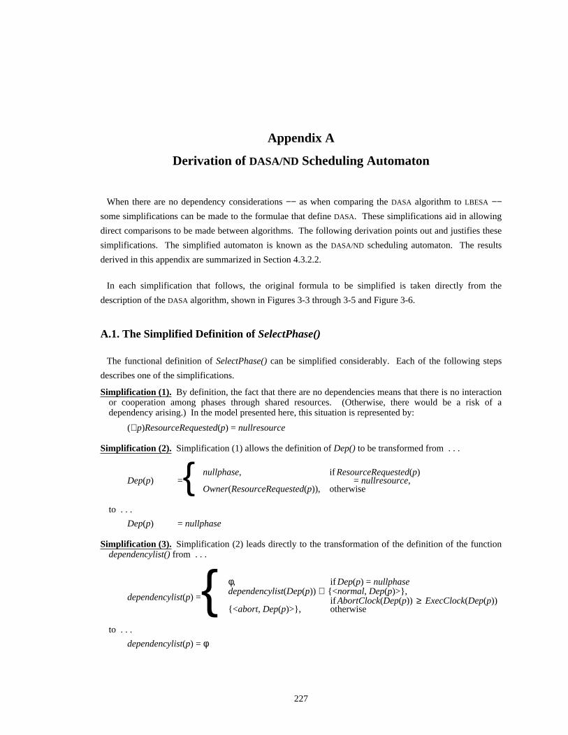
Appendix A
Derivation of DASA/ND Scheduling Automaton
When there are no dependency considerations −− as when comparing the DASA algorithm to LBESA −−some simplifications can be made to the formulae that define DASA. These simplifications aid in allowing
direct comparisons to be made between algorithms. The following derivation points out and justifies these
simplifications. The simplified automaton is known as the DASA/ND scheduling automaton. The results
derived in this appendix are summarized in Section 4.3.2.2.
In each simplification that follows, the original formula to be simplified is taken directly from the
description of the DASA algorithm, shown in Figures 3-3 through 3-5 and Figure 3-6.
A.1. The Simplified Definition of SelectPhase()
The functional definition of SelectPhase() can be simplified considerably. Each of the following steps
describes one of the simplifications.
Simplification (1). By definition, the fact that there are no dependencies means that there is no interactionor cooperation among phases through shared resources. (Otherwise, there would be a risk of adependency arising.) In the model presented here, this situation is represented by:
(∀p)ResourceRequested(p) = nullresource
Simplification (2). Simplification (1) allows the definition of Dep() to be transformed from . . .
nullphase, if ResourceRequested(p)Dep(p) = = nullresource,{ Owner(ResourceRequested(p)), otherwise
to . . .
Dep(p) = nullphase
Simplification (3). Simplification (2) leads directly to the transformation of the definition of the functiondependencylist() from . . .
φ, if Dep(p) = nullphasedependencylist(Dep(p)) ∪ {<normal, Dep(p)>},
dependencylist(p) = if AbortClock(Dep(p)) ≥ ExecClock(Dep(p)){{<abort, Dep(p)>}, otherwise
to . . .
dependencylist(p) = φ
227
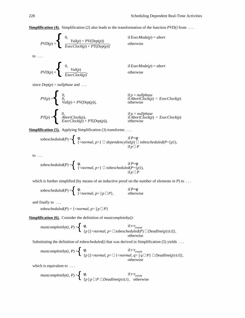
228 Scheduling Dependent Real-Time Activities
Simplification (4). Simplification (2) also leads to the transformation of the function PVD() from . . .
0, if ExecMode(p) = abortVal(p) + PV(Dep(p))
PVD(p) ={ , otherwiseExecClock(p) + PT(Dep(p))
to . . .
0, if ExecMode(p) = abortVal(p)
PVD(p) ={ , otherwiseExecClock(p)
since Dep(p) = nullphase and . . .
0, if p = nullphasePV(p) = 0, if AbortClock(p) < ExecClock(p){ Val(p) + PV(Dep(p)), otherwise
0, if p = nullphasePT(p) = AbortClock(p), if AbortClock(p) < ExecClock(p){ ExecClock(p) + PT(Dep(p)), otherwise
Simplification (5). Applying Simplification (3) transforms . . .
φ, if P=φtobescheduled(P) ={ {<normal, p>} ∪ dependencylist(p) ∪ tobescheduled(P−{p}),if p ∈ P
to . . .
φ, if P=φtobescheduled(P) ={ {<normal, p>} ∪ tobescheduled(P−{p}),if p ∈ P
which is further simplified (by means of an inductive proof on the number of elements in P) to . . .
φ, if P=φtobescheduled(P) ={ {<normal, p> | p ∈ P}, otherwise
and finally to . . .
tobescheduled(P) = {<normal, p> | p ∈ P}
Simplification (6). Consider the definition of mustcompleteby():
φ, if t<tmustcompleteby(t, P) = event{{p | [<normal, p> ∈ tobescheduled(P) ∧ Deadline(p) ≤ t]},
otherwise
Substituting the definition of tobescheduled() that was derived in Simplification (5) yields . . .
φ, if t<tmustcompleteby(t, P) = event{{p | [<normal, p> ∈ {<normal, q> | q ∈ P} ∧ Deadline(p) ≤ t]},
otherwise
which is equivalent to . . .
φ, if t<tmustcompleteby(t, P) = event{{p | p ∈ P ∧ Deadline(p) ≤ t}, otherwise
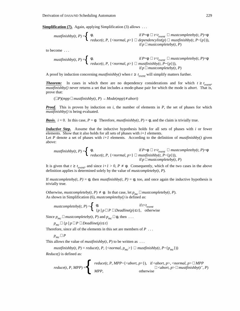
Derivation of DASA/ND Scheduling Automaton 229
Simplification (7). Again, applying Simplification (3) allows . . .
φ, if P=φ ∨ t<t ∨ mustcompleteby(t, P)=φmustfinishby(t, P) = event{reduce(t, P, {<normal, p>} ∪ dependencylist(p) ∪ mustfinishby(t, P−{p})),
if p ∈ mustcompleteby(t, P)
to become . . .
φ, if P=φ ∨ t<t ∨ mustcompleteby(t, P)=φmustfinishby(t, P) = event{reduce(t, P, {<normal, p>} ∪ mustfinishby(t, P−{p})),
if p ∈ mustcompleteby(t, P)
A proof by induction concerning mustfinishby() when t ≥ t will simplify matters further.event
Theorem: In cases in which there are no dependency considerations and for which t ≥ t ,eventmustfinishby() never returns a set that includes a mode-phase pair for which the mode is abort. That is,prove that:
(∀P)(mpp ∈ mustfinishby(t, P) → Mode(mpp) ≠ abort)
Proof. This is proven by induction on i, the number of elements in P, the set of phases for whichmustfinishby() is being evaluated.
Basis. i = 0. In this case, P = φ. Therefore, mustfinishby(t, P) = φ, and the claim is trivially true.
Inductive Step. Assume that the inductive hypothesis holds for all sets of phases with i or fewerelements. Show that it also holds for all sets of phases with i+1 elements.Let P denote a set of phases with i+1 elements. According to the definition of mustfinishby() givenabove:
φ, if P=φ ∨ t<t ∨ mustcompleteby(t, P)=φmustfinishby(t, P) = event{reduce(t, P, {<normal, p>} ∪ mustfinishby(t, P−{p})),
if p ∈ mustcompleteby(t, P)
It is given that t ≥ t , and since i+1 > 0, P ≠ φ. Consequently, which of the two cases in the aboveeventdefinition applies is determined solely by the value of mustcompleteby(t, P).
If mustcompleteby(t, P) = φ, then mustfinishby(t, P) = φ, too, and once again the inductive hypothesis istrivially true.
Otherwise, mustcompleteby(t, P) ≠ φ. In that case, let p ∈ mustcompleteby(t, P).mcAs shown in Simplification (6), mustcompleteby() is defined as:
φ, if t<tmustcompleteby(t, P) = event{{p | p ∈ P ∧ Deadline(p) ≤ t}, otherwise
Since p ∈ mustcompleteby(t, P) and p ∉ φ, then . . .mc mc
p ∈ {p | p ∈ P ∧ Deadline(p) ≤ t}mc
Therefore, since all of the elements in this set are members of P . . .
p ∈ Pmc
This allows the value of mustfinishby(t, P) to be written as . . .
mustfinishby(t, P) = reduce(t, P, {<normal, p >} ∪ mustfinishby(t, P−{p }))mc mc
Reduce() is defined as:
reduce(t, P, MPP−{<abort, p>}), if <abort, p>, <normal, p> ∈ MPP−reduce(t, P, MPP) = ∧ <abort, p> ∉ mustfinishby(t , P){ MPP, otherwise
230 Scheduling Dependent Real-Time Activities
It is given that P has i+1 elements, and it has been proven that p is one of them. Consequently,mcP−{p } has i elements and the inductive hypothesis asserts that . . .mc
mpp ∈ mustfinishby(t, P−{p }) → Mode(mpp) ≠ abortmc
Also, since Mode(<normal, p >) ≠ abort, the entire argument passed to the function reduce() containsmcno mode-phase pairs for which the mode is abort. Therefore, the second case in the definition ofreduce() applies, and reduce() acts as an identity function for this particular set of arguments . . .
reduce(t, P, {<normal, p >} ∪ mustfinishby(t, P−{p }))mc mc= {<normal, p >} ∪ mustfinishby(t, P−{p })mc mc
Inserting this fact into the earlier expression for mustfinishby(t,P) yields . . .
mustfinishby(t, P) = {<normal, p >} ∪ mustfinishby(t, P−{p })mc mc
Assume mpp ∈ mustfinishby(t, P). Using the definition for mustfinishby(t, P) that was just presented . . .
mpp ∈ {<normal, p >} ∪ mustfinishby(t, P−{p })mc mc
or equivalently . . .
mpp ∈ {<normal, p >} ∨ mpp ∈ mustfinishby(t, P−{p })mc mc
As was noted earlier, the set of phases P−{p } has i elements, so the inductive hypothesis holds andmcasserts . . .
mpp ∈ mustfinishby(t, P−{p }) → Mode(mpp) ≠ abortmc
Yet . . .
mpp ∉ mustfinishby(t, P−{p })mc→ mpp ∈ {<normal, p >}mc→ mpp = <normal, p >mc→ Mode(mpp) ≠ abort
Applying the following identity from formal logic, where the symbol " ≡ " denotes logical equivalenceand the symbol " ¬ " denotes logical negation:
(A → B) ∧ ( ¬ A → B) ≡ B
to the last two implications −− in which A is "mpp ∈ mustfinishby(t, P−{p })" and B ismc"Mode(mpp) ≠ abort" −− leads to the conclusion that:
Mode(mpp) ≠ abort
This conclusion −− that Mode(mpp) ≠ abort −− was derived by assuming mpp ∈ mustfinishby(t, P). Asecond rule of formal logic, the Deduction Theorem ( [Margaris 67]), states:
| |If ∆, A − B, then ∆ − A → B
|The terms to the left of the symbol "−" represent the set of assumptions that are made when proving theexpression to the right of the symbol. The Deduction Theorem, then, states that a statement, A, can beremoved from the set of assumptions if it is added as the antecedent of a conditional. Applying theDeduction Theorem where A is "mpp ∈ mustfinishby(t, P)" and B is "Mode(mpp) ≠ abort" proves that:
mpp ∈ mustfinishby(t, P) → Mode(mpp) ≠ abort
Therefore, the inductive hypothesis holds for all sets of phases P with i+1 members, whether or notmustcompleteby(t, P) is empty.
EndOfProof
Applying this result to the definition of mustfinishby(), once again noting that reduce() will always act asan identity function since . . .
(∀P)(mpp ∈ mustfinishby(t, P) → Mode(mpp) ≠ abort)
Derivation of DASA/ND Scheduling Automaton 231
yields . . .
φ, if P=φ ∨ t<t ∨ mustcompleteby(t, P)=φmustfinishby(t, P) = event{{<normal, p>} ∪ mustfinishby(t, P−{p})),
if p ∈ mustcompleteby(t, P)
Finally, a simple induction on the size of the set P will yield . . .
φ, if P=φ ∨ t<t ∨ mustcompleteby(t, P)=φmustfinishby(t, P) = event{{<normal, p> | p ∈ mustcompleteby(t, P)},
otherwise
Simplification (8). In the formulation of the DASA scheduling algorithm, the function timerequiredby() isonly evaluated with a result from mustfinishby() (ignoring the recursive evaluations that are part of thedefinition of timerequiredby()). As a short inductive proof would indicate, in that case timerequiredby()can be simplified since (as shown in Simplification (7)) mustfinishby() returns no mode-phase pairs thathave an abort mode. Therefore, timerequiredby() never receives an argument containing a mode-phasepair of the form <abort, p>, and it can be simplified from . . .
0, if MPP=φExecClock(p) + timerequiredby(MPP−{<normal, p>}),
timerequiredby(MPP) = if <normal, p> ∈ MPP{AbortClock(p) + timerequiredby(MPP−{<abort, p>}),
if <abort, p> ∈ MPP
to . . .
0, if MPP=φtimerequiredby(MPP) ={ ExecClock(p) + timerequiredby(MPP−{<normal, p>}),if <normal, p> ∈ MPP
Simplification (9). Pickone() is also only evaluated for an argument that is a result returned by evaluatingmustfinishby(). Once again, since mustfinishby() never returns a set containing an element that is amode-phase pair with an abort mode, pickone() can be simplified from . . .
<normal, p>, if <normal, p> ∈ MPP ∧ Dep(p) = nullphase<abort, p>, if <abort, p> ∈ MPP ∧ ¬ (∃q)
pickone(MPP) = (<normal, q> ∈ MPP ∧ Dep(q) = nullphase){<normal, nullphase>, otherwise
to . . .
<normal, p>, if <normal, p> ∈ MPP ∧ Dep(p) = nullphasepickone(MPP) ={ <normal, nullphase>, otherwise
Since, according to Simplification (2), (∀p)Dep(p) = nullphase . . .
<normal, p>, if <normal, p> ∈ MPPpickone(MPP) ={ <normal, nullphase>, otherwise
Finally, this function can be rewritten as . . .
<normal, nullphase>, if MPP = φpickone(MPP) ={ <normal, p> | <normal, p> ∈ MPP,otherwise
Simplification (10). As shown in Simplification (4) above . . .
0, if ExecMode(p) = abortVal(p)
PVD(p) ={ , otherwiseExecClock(p)
232 Scheduling Dependent Real-Time Activities
As shown in Simplification (9), pickone() will never return a mode-phase pair as a result whose mode isabort. As a result, the precondition for accepting an ‘abort-phase’ event for the DASA automaton willnever be satisfied. Since the postconditions of ‘abort-phase’ are the only way that ExecMode can bechanged to abort for any phase, then . . .
(∀p)ExecMode(p) = normal
This allows the first case in the definition of PVD() to be dropped, yielding . . .
Val(p)PVD(p) =
ExecClock(p)
A.2. The Simplified Definition of the Automaton
There are also a set of simplifications that can be made to the automaton itself when there are no
dependencies to consider. Each of these simplifications are discussed in turn.
Simplification (1). As pointed out before, all of the simplifications stem from the fact that . . .
(∀p)ResourceRequested(p) = nullresource
Consider the postconditions defined for a ‘request’ event:
ExecClock′(p) = ExecClock(p) − (t − ResumeTime(p))aResourceRequested′(p) = r ; indicate p is resource-waitingPhaseElect′ = SelectPhase(PhaseList)RunningPhase = nullphase ; give up processor until ‘grant’ed resource
They necessarily include an assignment to ResourceRequested for some phase, it must be the case that no‘request’ event can be accepted by the simplified DASA automaton. Therefore, the precondition for theacceptance of a ‘request’ event is false, and the event can be eliminated from the automaton.
Simplification (2). Similarly, consider the precondition for the acceptance of a ‘grant’ event:
(RunningPhase = nullphase) ∧ (Phase(PhaseElect) = p) ∧ (r ≠ nullresource)∧ (ResourceRequested(Phase(PhaseElect)) = r) ∧ (Mode(PhaseElect) = normal)
Since it includes as conjuncts (ResourceRequested(Phase(PhaseElect)) = r) and (r ≠ nullresource), thisprecondition can never be satisfied because (∀p)ResourceRequested(p) = nullresource. Therefore, thisprecondition will always be false, a ‘grant’ event can never be accepted, and the event can be eliminatedfrom the simplified DASA automaton.
Simplification (3). Consider the precondition for the acceptance of a ‘resume-phase’ event:
(RunningPhase = nullphase) ∧ (Phase(PhaseElect) = p) ∧ (Phase(PhaseElect) ≠ nullphase)∧ ¬ ResourceWaiting(Phase(PhaseElect)) ∧ (Mode(PhaseElect) = normal)
In particular, consider the conjunct ¬ ResourceWaiting(Phase(PhaseElect)), remembering that, bydefinition . . .
ResourceWaiting(p) ≡ (∃r)(ResourceRequested(p)=r ∧ r ≠ nullresource ∧ Owner(r) ≠ p)
ResourceWaiting() must be false for all phases, implying that ¬ ResourceWaiting(p) must be true for allphases p. Therefore, the precondition for the acceptance of a ‘resume-phase’ event may be simplified to:
(RunningPhase = nullphase) ∧ (Phase(PhaseElect) = p) ∧ (Phase(PhaseElect) ≠ nullphase)∧ (Mode(PhaseElect) = normal)
Simplification (4). The postconditions associated with a ‘request-phase’ event include:
;release the resources acquired during the phasefor r in ResourcesHeld(p)
Owner′(r) = φResourcesHeld′(p) = φ
Derivation of DASA/ND Scheduling Automaton 233
ResourcesHeld is initially set to φ and is only altered by the postconditions accompanying the acceptanceof a ‘grant’ event. Since it was shown in simplification 2, that there can be no ‘grant’ events, then theseactions concerning ResourcesHeld in the postconditions for a ‘request-phase’ have no effect.Furthermore, Owner is initially set to nullphase and is only changed as a result of the postconditions thataccompany the acceptance of a ‘grant’ event. Consequently, all of the postconditions listed immediatelyabove can be eliminated from the simplified DASA automaton without ill-effect. In fact, the statecomponents Owner, ResourcesHeld, and ResourceRequested can all be eliminated from the automaton aswell.
Simplification (5). Consider the precondition for the acceptance of an ‘abort-phase’ event:
(RunningPhase = nullphase) ∧ (Phase(PhaseElect) = p) ∧ (Mode(PhaseElect) = abort)
In particular, consider the conjunct (Mode(PhaseElect) = abort). PhaseElect always receives its value asa result of the following evaluation:
PhaseElect′ = SelectPhase(PhaseList′)and . . .
SelectPhase(P) = pickone( mustfinishby(DL (mpplist), P (P)) ),first scheduledwhere
mpplist = tobescheduled(P (P))scheduled
<normal, nullphase>, if MPP = φpickone(MPP) ={ <normal, p> | <normal, p> ∈ MPP,otherwise
Under no circumstances will this return a mode-phase pair with a mode indicating abort. Therefore, theconjunct (Mode(PhaseElect) = abort) will always be false and the entire precondition is always false.Consequently, the entire ‘abort-phase’ portion of the DASA automaton may be omitted in the simplifiedversion.
Simplification (6). Simplification (10) of Section A.1 shows that:
(∀p)ExecMode(p) = normal
This fact can be applied to the postconditions of the ‘request-phase’ event to transform:
if (ExecMode(RunningPhase) = normal) thenExecClock’(RunningPhase)
= ExecClock(RunningPhase) - (t - ResumeTime(RunningPhase))eventelse
AbortClock’(RunningPhase)= AbortClock(RunningPhase) - (t - ResumeTime(RunningPhase))event
endif
into:
ExecClock’(RunningPhase)= ExecClock(RunningPhase) - (t - ResumeTime(RunningPhase))event
Simplification (7). This time the fact that ExecMode(p) is always normal is applied to the postconditionsof the ‘preempt-phase’ event to transform:
if (ExecMode(p) = normal) thenExecClock’(p) = ExecClock(p) - (t - ResumeTime(p))event
elseAbortClock’(p) = AbortClock(p) - (t - ResumeTime(p))event
endif
into:
ExecClock’(p) = ExecClock(p) - (t - ResumeTime(p))event

234 Scheduling Dependent Real-Time Activities
References 235
References
[Abbott 87] Abbott, R. and Garcia-Molina, H.Scheduling Real-Time Transactions.Technical Report CS-TR-129-87, Princeton University, Department of Computer
Science, Princeton, NJ, 1987.
[Abbott 89] Abbott, R. and Garcia-Molina, H.Scheduling Real-Time Transactions with Disk Resident Data.Technical Report CS-TR-207-89, Princeton University, Department of Computer
Science, Princeton, NJ, 1989.
[AHU 74] Aho, A. V., Hopcroft, J. E. and Ullman, J. D.Addison-Wesley Series in Computer Science and Information Processing: The Design
and Analysis of Computer Algorithms.Addison-Wesley Publishing Company, 1974.
[Alpha 88] Northcutt, J. D. and Clark, R. K.The Alpha Operating System: Programming Model.Technical Report Archons Project Technical Report TR #88021, Carnegie Mellon
University, Department of Computer Science, Pittsburgh, PA, 1988.
[Alpha 90] Trull, J., Northcutt, J. D., Maynard, D. P. and Clark, R. K.The Alpha Operating System: Scheduler Evaluation Experiments.Technical Report Archons Project Technical Report TR #90021, Carnegie Mellon
University, Department of Computer Science, Pittsburgh, PA, 1990.
[Bach 86] Bach, M. J.The Design of the UNIX Operating System.Prentice-Hall, Inc., 1986.
[Baker 74] Baker, K. R.Introduction to Sequencing and Scheduling.John Wiley & Sons, 1974.
[Baker 86] Baker, J. M.Structured Systems Development for Real-Time Systems.In National Conference and Workshop on Methodologies and Tools for Real-Time
Systems. The National Institute for Software Quality and Productivity, March, 1986.
[Bennett 88] Bennett, S.Prentice Hall International Series in Systems and Control Engineering: Real-Time
Computer Control: An Introduction.Prentice Hall, 1988.
[BHG 87] Bernstein, P. A., Hadzilacos, V. and Goodman, N.Concurrency Control and Recovery in Database Systems.Addison-Wesley Publishing Company, 1987.
236 Scheduling Dependent Real-Time Activities
[Birman 88] Birman, K. P. and Joseph, T. A.Exploiting Replication.Technical Report TR 88-917, Cornell University, Department of Computer Science,
Ithaca, NY, June, 1988.This is a preprint of material that will appear in the collected lecture notes from ’Arctic
88, An Advanced Course on Operating Systems’, Tromso, Norway, July 5-14, 1988.The lecture notes will appear in book form later this year.
[Blazewicz 77] Blazewicz, J.Scheduling Dependent Tasks with Different Arrival Times to Meet Deadlines.Modelling and Performance Evaluation of Computer Systems.North-Holland Publishing Company, 1977.Proceedings of the International Workshop organized by the Commission of the
European Communities, Joint Research Centre, Ispra Establishment, Department A,Ispra (Varese), Italy, October 4-6, 1976.
[Cheng 86] Cheng, S., Stankovic, J. A. and Ramamritham, K.Dynamic Scheduling of Groups of Tasks with Precedence Constraints in Distributed
Hard Real-Time Systems.In Proceedings of the Real-Time Systems Symposium, pages 166-174. December, 1986.
[CMUGD 90] Maynard, D. P., Clark, R. K., Northcutt, J. D., Shipman, S. E., Kegley, R. B., Keheler,P. J., Zimmerman, B. A. and Jensen, E. D.The Alpha Operating System: An Example Command, Control, and Battle Management
Application.Technical Report Archons Project Technical Report, Carnegie Mellon University,
Department of Computer Science, Pittsburgh, PA, To appear: 1990.
[Conway 67] Conway, R. W., Maxwell, W. L. and Miller, L. W.Theory of Scheduling.Addison-Wesley Publishing Company, 1967.
[CRC 87] Chemical Rubber Company.CRC Standard Mathematical Tables, 28th Edition.CRC Press, 1987.
[Date 86] Date, C. J.Addison-Wesley Systems Programming Series. Volume I: An Introduction to Database
Systems, Fourth Edition.Addison-Wesley Publishing Company, 1986.
[DEI 85] Dravo Engineers, Inc.USS Gary Works Level 2 Computer Control System: System Design Document, Volumes
I and II.Technical Report, Dravo Engineers, Incorporated, Pittsburgh, PA, July/August, 1985.
[DLRK 81] Dempster, M. A. H., Lenstra, J. K. and Rinnooy Kan, A. H. G. (editors).Deterministic and Stochastic Scheduling.D. Reidel Publishing Company, 1981.Proceedings of the NATO Advanced Study and Research Institute on Theoretical
Approaches to Scheduling Problems, held in Durham, England, July 6-17, 1981.
[Elsayed 82] Elsayed, E. A.Algorithms for Project Scheduling with Resource Constraints.International Journal of Production Research 20(1):95-103, January/February, 1982.
[Eswaran 76] Eswaran, K. P., Gray, J. N., Lorie, R. A. and Traiger, I. L.The Notions of Consistency and Predicate Locks in a Database System.Communications of the ACM 19(11):624-633, November, 1976.
References 237
[French 82] French, S.Sequencing and Scheduling: An Introduction to the Mathematics of the Job-Shop.John Wiley & Sons, 1982.
[GD 80] General Dynamics.Computer Program Product Specification for the System Function Processor
Operational Flight Program for the F-16 Multinational Staged ImprovementProgram, Block 30.
Technical Report CPCI 7175-1A00, General Dynamics Corporation, December, 1980.
[Gittins 81] Gittins, J. C.Forwards Induction and Dynamic Allocation Indices.In Deterministic and Stochastic Scheduling: Proceedings of the NATO Advanced Study
and Research Institute on Theoretical Approaches to Scheduling Problems, pages125-156. July, 1981.
[Hatley 86] Hatley, D. J.Structured Methods for Large Avionics Systems.In National Conference and Workshop on Methodologies and Tools for Real-Time
Systems. The National Institute for Software Quality and Productivity, March, 1986.
[Herlihy 87] Herlihy, M.Concurrency versus Availability: Atomicity Mechanisms for Replicated Data.ACM Transactions on Computer Systems 5(3):249-274, August, 1987.
[Herlihy 88] Herlihy, M. P.Impossibility and Universality Results for Wait-Free Synchronization.Technical Report CMU-CS-88-140, Carnegie Mellon University, Computer Science
Department, Pittsburgh, PA, May, 1988.
[HiPAC 88] Dayal, U., Blaustein, B., Buchmann, A., Chakravarthy, U., Hsu, M., Ledin, R.,McCarthy, D., Rosenthal, A., Sarin, S. Carey, M. J., Livny, M. and Jauhari, R.The HiPAC Project: Combining Active Databases and Timing Constraints.ACM SIGMOD Record 17(1):51-70, March, 1988.
[Janson 85] Janson, P. A.Operating Systems: Structures and Mechanisms.Academic Press, 1985.
[Jensen 75] Jensen, E. D.Time-Value Functions for BMD Radar Scheduling.Technical Report, Honeywell Systems and Research Center, June, 1975.
[Jensen 76a] Jensen, E. D.Distributed Processing in a Real-Time Environment.Infotech State of the Art Report on Distributed Systems.Infotech International Ltd., 1976, pages 304-318.
[Jensen 76b] Jensen, E. D.Decentralized Operating Systems.In Workshop on Distributed Processing. Brown University, August, 1976.
[Jensen 88] Jensen, E. D.Alpha Objectives and Requirements.Part of Alpha Preview: A Briefing and Technology Demonstration for DoD.March, 1988
238 Scheduling Dependent Real-Time Activities
[Joseph 88] Joseph, T. A. and Birman, K. P.Reliable Broadcast Protocols.Technical Report TR 88-918, Cornell University, Department of Computer Science,
Ithaca, NY, June, 1988.This is a preprint of material that will appear in the collected lecture notes from ’Arctic
88, An Advanced Course on Operating Systems’, Tromso, Norway, July 5-14, 1988.The lecture notes will appear in book form later this year.
[KB 84] Kenah, L. J. and Bate, S. F.VAX/VMS Internals and Data Structures.Digital Press, 1984.
[Knapp 87] Knapp, E.Deadlock Detection in Distributed Databases.ACM Computing Surveys 19(4):303-328, December, 1987.
[Lawler 73] Lawler, E. L.Optimal Sequencing of a Single Machine Subject to Precedence Constraints.Management Science 19(5):544-546, January, 1973.
[Liskov 83] Liskov, B. and Scheifler, R.Guardians and Actions: Linguistic Support for Robust, Distributed Programs.ACM Transactions on Programming Languages and Systems 5(3):381-404, July, 1983.
[Liu 73] Liu, C. L. and Layland, J. W.Scheduling Algorithms for Multiprogramming in a Hard-Real-Time Environment.Journal of the Association for Computing Machinery 20(1):46-61, January, 1973.
[Liu 88] Liu, J. W. S., Lin, K. J. and Song, X.Scheduling Hard Real-Time Transactions.The Fifth Workshop on Real-Time Software and Operating Systems :112-116, May,
1988.
[Locke 86] Locke, C. D.Best-Effort Decision Making for Real-Time Scheduling.PhD thesis, Carnegie Mellon University, May, 1986.
[Mach 86] Accetta, M., Baron, R., Bolosky, W., Golub, D., Rashid, R., Tevanian, A., and Young,M.Mach: A New Kernel Foundation for UNIX Development.In Proceedings of Summer Usenix. July, 1986.
[MacLaren 80] MacLaren, L.Evolving Toward Ada in Real-Time Systems.ACM SIGPLAN Notices 15(11):146-155, November, 1980.This issue was also the Proceedings of the ACM-SIGPLAN Symposium on the Ada
Programming Language, Boston, MA; December 9-11, 1980.
[Margaris 67] Margaris, A.First Order Mathematical Logic.Xerox College Publishing, 1967.
[Martel 82] Martel, C.Preemptive Scheduling with Release Times, Deadlines, and Due Dates.Journal of the Association for Computing Machinery 29(3):812-829, July, 1982.
[Maynard 91] Maynard, D. P.Time-Driven Scheduling of Composite Real-Time Activities.PhD thesis, Carnegie Mellon University, To appear: 1991.
[McKendry 85] McKendry, M. S.Ordering Actions for Visibility.Transactions on Software Engineering (IEEE) 11(6):509-519, June, 1985.
References 239
[Moore 68] Moore, J. M.An n Job, One Machine Sequencing Algorithm for Minimizing the Number of Late Jobs.Management Science 15(1):102-109, September, 1968.
[Northcutt 87] Northcutt, J. D.Perspectives in Computing Series. Volume 16: Mechanisms for Reliable Distributed
Real-Time Operating Systems: The Alpha Kernel.Academic Press, 1987.
[Peterson 85] Peterson, J. L. and Silberschatz, A.Operating System Concepts, Second Edition.Addison-Wesley Publishing Company, 1985.
[Rajkumar 89] Rajkumar, R.Task Synchronization in Real-Time Systems.PhD thesis, Carnegie Mellon University, August, 1989.
[Ramamritham 84]Ramamritham, K. and Stankovic, J. A.Dynamic Task Scheduling in Hard Real-Time Distributed Systems.IEEE Software 1(3):65-75, July, 1984.
[Rauch-Hindin 87]Rauch-Hindin, W. B.UNIX Overcomes Its Real-Time Limitations.UNIX World 4(11):64-78, November, 1987.
[Ritchie 74] Ritchie, D. M. and Thompson, K.The UNIX Time-Sharing System.Communications of the ACM 17(7):365-375, July, 1974.
[Sha 85] Sha, L.Modular Concurrency Control and Failure Recovery --- Consistency, Correctness and
Optimality.PhD thesis, Carnegie Mellon University, 1985.
[Sha 86] Sha, L., Lehoczky, J. P. and Rajkumar, R.Solutions for Some Practical Problems in Prioritized Preemptive Scheduling.In Proceedings of the Real-Time Systems Symposium, pages 181-191. December, 1986.
[Sha 87] Sha, L., Rajkumar, R. and Lehoczky, J. P.Priority Inheritance Protocols: An Approach to Real-Time Synchronization.Technical Report CMU-CS-87-181, Carnegie Mellon University, Computer Science
Department, Pittsburgh, PA, December, 1987.
[Sha 90] Sha, L. and Goodenough, J. B.Real-Time Scheduling Theory and Ada.IEEE Computer 23(4):53-62, April, 1990.
[Stadick 83] Stadick, E. M.A Real-Time Control System Implementation Study Using the Ada Programming
Language.Technical Report NSWC TR-83-213, Naval Surface Weapons Center, 1983.
[Stankovic 88] Stankovic, J. A. and Zhao, W.On Real-Time Transactions.ACM SIGMOD Record 17(1):4-18, March, 1988.
[Ullman 75] Ullman, J. D.NP-Complete Scheduling Problems.Journal of Computer and System Sciences 10(3):384-393, June, 1975.

240 Scheduling Dependent Real-Time Activities
[Zhao 87] Zhao, W., Ramamritham, K., and Stankovic, J. A.Scheduling Tasks with Resource Requirements in Hard Real-Time Systems.IEEE Transactions on Software Engineering SE-13(5):564-577, May, 1987.
Table of Contents i
Table of Contents
1. Introduction 11.1. Problem Definition 2
1.1.1. Dependencies 31.1.2. Real-Time Systems 4
1.2. Schedulers and Scheduling Information 71.3. Scheduling Example 101.4. Motivation for Using Application-Defined Values 11
1.4.1. Accrued Value 121.4.2. Time-Value Functions 14
1.5. Technical Approach 151.5.1. Define Model 151.5.2. Devise Algorithms 151.5.3. Prove Properties Analytically 161.5.4. Simulate Algorithm 16
2. The Scheduling Model 172.1. Informal Model and Rationale 17
2.1.1. Applications, Activities, and Phases 172.1.2. Shared Resources 182.1.3. Phase Preemption 192.1.4. Phase Abortion 192.1.5. Events 202.1.6. Histories 212.1.7. Scheduling Automata 22
2.1.7.1. General Structure 232.1.7.2. Specific Scheduling Automata 24
2.2. Assumptions and Restrictions of Model 252.3. Formal Model 25
2.3.1. Notation and Definitions 262.3.1.1. Naming Conventions 262.3.1.2. Mode-Phase Pairs 262.3.1.3. Time-Value Functions 26
2.3.2. The General Scheduling Automaton Framework (GSAF) 272.3.2.1. Applications and Activities 272.3.2.2. Events and Histories 272.3.2.3. Operations 282.3.2.4. Computational Phases of Activities 292.3.2.5. Shared Resources 292.3.2.6. Phase Preemption and Resumption 292.3.2.7. Event Terminology and Notation 302.3.2.8. Definitions and Properties of Histories 302.3.2.9. Automaton State Components 322.3.2.10. Operations Accepted by GSAF with Preconditions and Postconditions 352.3.2.11. Active Phase Selection 38
ii Scheduling Dependent Real-Time Activities
2.3.3. Notes 392.3.3.1. Manifestation of Assumptions and Restrictions 392.3.3.2. Manifestation of Interrupts 402.3.3.3. Atomic Nature of ‘Request-Phase’ Events 40
2.4. Observations on the Model 403. The DASA Algorithm 43
3.1. Dependent Activity Scheduling Algorithm 433.1.1. Heuristics and Rationale 433.1.2. Informal Definition of DASA 44
3.1.2.1. Dependency Scheduling 453.1.2.2. Deadlock Resolution 46
3.2. Formal Definition of DASA 463.2.1. The Formal Definition 46
3.2.1.1. DASA Automaton State Components 473.2.1.2. Operations Accepted by DASA Automaton 483.2.1.3. SelectPhase() Function for DASA Automaton 55
3.2.2. Observations on the Definition 603.2.2.1. Manifestation of Desirable Properties 603.2.2.2. Nondeterminism in Definition 613.2.2.3. Explicit Appearance of Time 62
3.3. Scheduling Example Revisited 624. Analytic Results 65
4.1. Requirements for Scheduling Algorithms 654.2. Strategy for Demonstrating Requirement Satisfaction 664.3. Proofs of Properties 66
4.3.1. Algorithm Correctness 674.3.1.1. Proof: Selected Phases May Execute Immediately 67
4.3.2. Algorithm Value 684.3.2.1. LBESA Scheduling Automaton 684.3.2.2. DASA/ND Scheduling Automaton 714.3.2.3. Proof: If No Overloads, DASA and LBESA Are Equivalent 754.3.2.4. Proof: With Overloads, DASA May Exceed LBESA 80
4.3.3. Algorithm Tractability 1104.3.3.1. Procedural Version of DASA 1104.3.3.2. Proof: Procedural Version of DASA Is Polynomial in Space and Time 114
4.4. Notes on Algorithm 1164.4.1. Unbounded Value Density Growth 1164.4.2. Idle Intervals During Overload 1174.4.3. Cleverness and System Dynamics 119
5. Simulation Results 1215.1. Simulator Design and Implementation 121
5.1.1. Requirements 1225.1.2. Design 122
5.1.2.1. Activities and the Activity Generator 1235.1.2.2. Integrated Scheduler 124
5.1.3. Implementation 1245.1.3.1. Approach: Build from Scratch or Adapt an Existing Simulator 1245.1.3.2. Source of DASA Implementation 1255.1.3.3. Single Scheduler for Simulation 1265.1.3.4. Simulator Display Messages 1265.1.3.5. Modifications 127
5.2. Evaluation of DASA Decisions 1285.2.1. Methods of Evaluation 128
Table of Contents iii
5.2.1.1. Execute Existing Applications 1285.2.1.2. Modifying or Reimplementing Existing Applications 1305.2.1.3. Modeling Existing Applications 1305.2.1.4. Simulating the Execution of a Parameterized Application 131
5.2.2. Workload Selection 1315.2.2.1. Arrival Times, Required Computation Times, and Values 1325.2.2.2. Shared Resources 132
5.2.3. Examination of DASA Behavior 1335.2.3.1. Workload Parameters and Metrics 1335.2.3.2. Scheduler Performance Analysis: U/U Distribution 1365.2.3.3. Scheduler Performance Analysis: M/M Distribution 140
5.3. Evaluation of DASA With Scheduling Overhead 1425.3.1. Low Overhead 1445.3.2. Medium Overhead 1445.3.3. High Overhead 1455.3.4. Summary 145
5.4. Evaluation of DASA Abort Usage 1465.5. Interpreting Simulation Results for Specific Applications 148
5.5.1. Telephone Switching 1485.5.2. Process Control: A Steel Mill 150
6. Related Work and Current Practice 2036.1. Priority-Based Scheduling 2046.2. Deadline-Based and Time-Driven Scheduling 2056.3. Other Related Work 207
7. Future Work 2097.1. Loosening Assumptions 209
7.1.1. Known Computation Time for Phase 2097.1.2. Exclusive Access to Shared Resources 2107.1.3. Simple Time-Value Functions 211
7.2. Generalizing the Model 2127.2.1. Multiprocessor Scheduling 2127.2.2. Multiple Node Scheduling 2137.2.3. Grouped Resource Requests 2137.2.4. Release of Shared Resources 2147.2.5. Nested Phases 215
7.3. Transitioning DASA into Practice 2167.3.1. Efficient Scheduler Execution 2167.3.2. Deadlock Detection and Resolution 2187.3.3. Prior Experience and Future Plans 219
7.4. Exploring Algorithmic Variations 2207.4.1. Dependency List Variations 2207.4.2. Value Metric Variations 2207.4.3. Overload Variations 221
7.5. Analyzing DASA for Specific Applications 2217.5.1. Further Simulations 2217.5.2. Real Applications 222
8. Conclusions 2238.1. Contributions 2238.2. Summary 226
Appendix A. Derivation of DASA/ND Scheduling Automaton 227A.1. The Simplified Definition of SelectPhase() 227A.2. The Simplified Definition of the Automaton 232

iv Scheduling Dependent Real-Time Activities
References 235
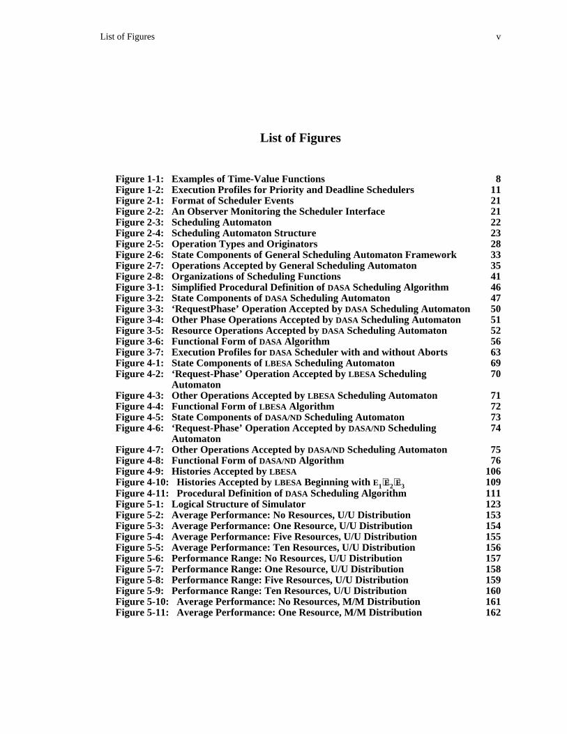
List of Figures v
List of Figures
Figure 1-1: Examples of Time-Value Functions 8Figure 1-2: Execution Profiles for Priority and Deadline Schedulers 11Figure 2-1: Format of Scheduler Events 21Figure 2-2: An Observer Monitoring the Scheduler Interface 21Figure 2-3: Scheduling Automaton 22Figure 2-4: Scheduling Automaton Structure 23Figure 2-5: Operation Types and Originators 28Figure 2-6: State Components of General Scheduling Automaton Framework 33Figure 2-7: Operations Accepted by General Scheduling Automaton 35Figure 2-8: Organizations of Scheduling Functions 41Figure 3-1: Simplified Procedural Definition of DASA Scheduling Algorithm 46Figure 3-2: State Components of DASA Scheduling Automaton 47Figure 3-3: ‘RequestPhase’ Operation Accepted by DASA Scheduling Automaton 50Figure 3-4: Other Phase Operations Accepted by DASA Scheduling Automaton 51Figure 3-5: Resource Operations Accepted by DASA Scheduling Automaton 52Figure 3-6: Functional Form of DASA Algorithm 56Figure 3-7: Execution Profiles for DASA Scheduler with and without Aborts 63Figure 4-1: State Components of LBESA Scheduling Automaton 69Figure 4-2: ‘Request-Phase’ Operation Accepted by LBESA Scheduling 70
AutomatonFigure 4-3: Other Operations Accepted by LBESA Scheduling Automaton 71Figure 4-4: Functional Form of LBESA Algorithm 72Figure 4-5: State Components of DASA/ND Scheduling Automaton 73Figure 4-6: ‘Request-Phase’ Operation Accepted by DASA/ND Scheduling 74
AutomatonFigure 4-7: Other Operations Accepted by DASA/ND Scheduling Automaton 75Figure 4-8: Functional Form of DASA/ND Algorithm 76Figure 4-9: Histories Accepted by LBESA 106Figure 4-10: Histories Accepted by LBESA Beginning with E ⋅E ⋅E 1091 2 3Figure 4-11: Procedural Definition of DASA Scheduling Algorithm 111Figure 5-1: Logical Structure of Simulator 123Figure 5-2: Average Performance: No Resources, U/U Distribution 153Figure 5-3: Average Performance: One Resource, U/U Distribution 154Figure 5-4: Average Performance: Five Resources, U/U Distribution 155Figure 5-5: Average Performance: Ten Resources, U/U Distribution 156Figure 5-6: Performance Range: No Resources, U/U Distribution 157Figure 5-7: Performance Range: One Resource, U/U Distribution 158Figure 5-8: Performance Range: Five Resources, U/U Distribution 159Figure 5-9: Performance Range: Ten Resources, U/U Distribution 160Figure 5-10: Average Performance: No Resources, M/M Distribution 161Figure 5-11: Average Performance: One Resource, M/M Distribution 162
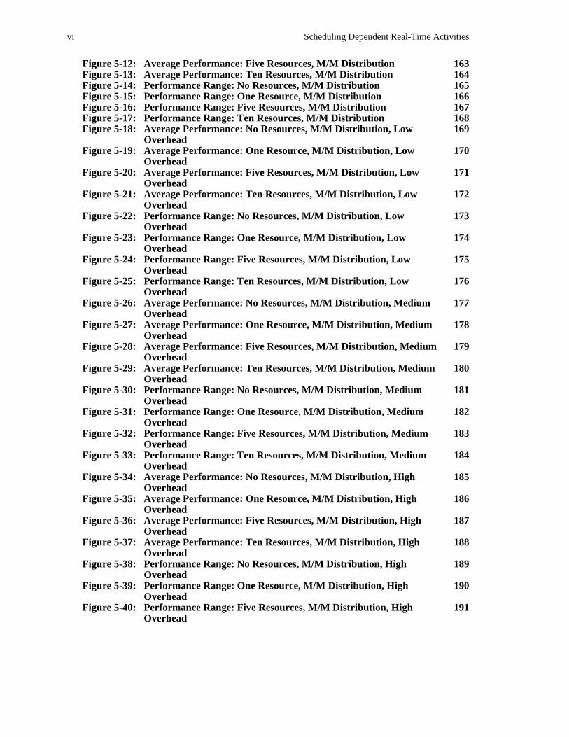
vi Scheduling Dependent Real-Time Activities
Figure 5-12: Average Performance: Five Resources, M/M Distribution 163Figure 5-13: Average Performance: Ten Resources, M/M Distribution 164Figure 5-14: Performance Range: No Resources, M/M Distribution 165Figure 5-15: Performance Range: One Resource, M/M Distribution 166Figure 5-16: Performance Range: Five Resources, M/M Distribution 167Figure 5-17: Performance Range: Ten Resources, M/M Distribution 168Figure 5-18: Average Performance: No Resources, M/M Distribution, Low 169
OverheadFigure 5-19: Average Performance: One Resource, M/M Distribution, Low 170
OverheadFigure 5-20: Average Performance: Five Resources, M/M Distribution, Low 171
OverheadFigure 5-21: Average Performance: Ten Resources, M/M Distribution, Low 172
OverheadFigure 5-22: Performance Range: No Resources, M/M Distribution, Low 173
OverheadFigure 5-23: Performance Range: One Resource, M/M Distribution, Low 174
OverheadFigure 5-24: Performance Range: Five Resources, M/M Distribution, Low 175
OverheadFigure 5-25: Performance Range: Ten Resources, M/M Distribution, Low 176
OverheadFigure 5-26: Average Performance: No Resources, M/M Distribution, Medium 177
OverheadFigure 5-27: Average Performance: One Resource, M/M Distribution, Medium 178
OverheadFigure 5-28: Average Performance: Five Resources, M/M Distribution, Medium 179
OverheadFigure 5-29: Average Performance: Ten Resources, M/M Distribution, Medium 180
OverheadFigure 5-30: Performance Range: No Resources, M/M Distribution, Medium 181
OverheadFigure 5-31: Performance Range: One Resource, M/M Distribution, Medium 182
OverheadFigure 5-32: Performance Range: Five Resources, M/M Distribution, Medium 183
OverheadFigure 5-33: Performance Range: Ten Resources, M/M Distribution, Medium 184
OverheadFigure 5-34: Average Performance: No Resources, M/M Distribution, High 185
OverheadFigure 5-35: Average Performance: One Resource, M/M Distribution, High 186
OverheadFigure 5-36: Average Performance: Five Resources, M/M Distribution, High 187
OverheadFigure 5-37: Average Performance: Ten Resources, M/M Distribution, High 188
OverheadFigure 5-38: Performance Range: No Resources, M/M Distribution, High 189
OverheadFigure 5-39: Performance Range: One Resource, M/M Distribution, High 190
OverheadFigure 5-40: Performance Range: Five Resources, M/M Distribution, High 191
Overhead
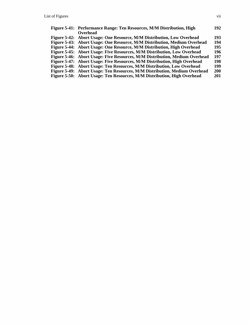
List of Figures vii
Figure 5-41: Performance Range: Ten Resources, M/M Distribution, High 192Overhead
Figure 5-42: Abort Usage: One Resource, M/M Distribution, Low Overhead 193Figure 5-43: Abort Usage: One Resource, M/M Distribution, Medium Overhead 194Figure 5-44: Abort Usage: One Resource, M/M Distribution, High Overhead 195Figure 5-45: Abort Usage: Five Resources, M/M Distribution, Low Overhead 196Figure 5-46: Abort Usage: Five Resources, M/M Distribution, Medium Overhead 197Figure 5-47: Abort Usage: Five Resources, M/M Distribution, High Overhead 198Figure 5-48: Abort Usage: Ten Resources, M/M Distribution, Low Overhead 199Figure 5-49: Abort Usage: Ten Resources, M/M Distribution, Medium Overhead 200Figure 5-50: Abort Usage: Ten Resources, M/M Distribution, High Overhead 201

viii Scheduling Dependent Real-Time Activities
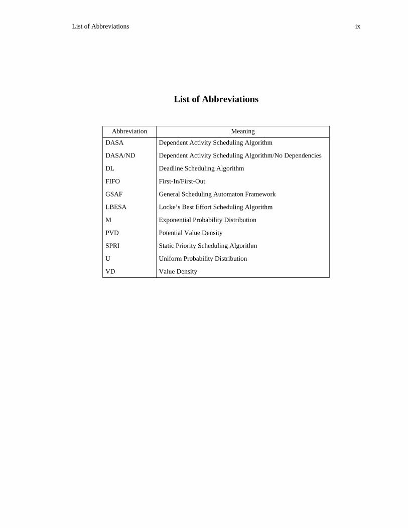
List of Abbreviations ix
List of Abbreviations
Abbreviation Meaning
DASA Dependent Activity Scheduling Algorithm
DASA/ND Dependent Activity Scheduling Algorithm/No Dependencies
DL Deadline Scheduling Algorithm
FIFO First-In/First-Out
GSAF General Scheduling Automaton Framework
LBESA Locke’s Best Effort Scheduling Algorithm
M Exponential Probability Distribution
PVD Potential Value Density
SPRI Static Priority Scheduling Algorithm
U Uniform Probability Distribution
VD Value Density

x Scheduling Dependent Real-Time Activities
List of Symbols xi
List of Symbols
Symbol Meaning
∧ Logical And
∨ Logical Or
¬ Logical Negation
≡ Logical Equivalence
→ Logical Implication
|A − B B can be derived given assumptions A
(a, b) open interval extending from ‘a’ to ‘b’

xii Scheduling Dependent Real-Time Activities