INF 5460 Electronic noise – estimates and countermeasures

Mandatory 3 – Introduction to CMOS in LTspice

Simulation modes

Time Frequency

Signal(standard)

.TRAN .AC

Component noise

.TRAN V (added by user: standard sources or from file).NOISETRAN (noise sources generated by software)

.NOISE (noise sources generated by software)

Coupling noise

.TRAN--- V (manually added by user: standard V-sources or from file) --- R, C or L modelling parasitic (Extracted by software or manually added by user)

.AC--- V (manually added by user: AC)--- R, C or L modelling parasitic (Extracted by software or manually added by user)

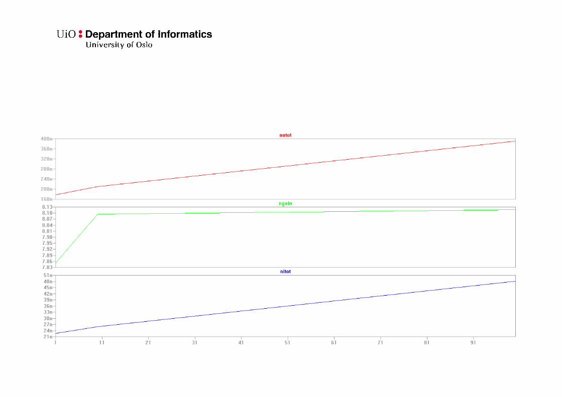
Transient component noise simulation

Four simulations:• No noise

• Source resistor noise

• Feedback resistor noise

• Noise from both resistors

LTspice: Preparing CMOS model for mandatory 3

• Will use transistor models for an integrated circuit process: 0.35µm CMOS from AMS (Austria Micro Systems)

• Preparation:1. Include transistor model

2. Include symbols

3. Set correct transistor model for transistors in schematic

4. Set correct length and width for transistors in schematic

LTspice: Preparing CMOS model1 Generally a transistor models can be included as:

– A model in the standard model library file,

– As a private library file. Must include link in the schematic, or

– As “text” in the schematic

We chose the first alternative and replace <program files>/LTC/LTspiceIV/lib/cmp/standard.mos with our own file

2 Transistor symbols– We use our own transistor symbols (that show widths, lengths etc.).

They must be on the same directory as we have our schematics.

LTspice: Preparing CMOS model

3 Correct transistor model– Change the transistor model name for NMOS transistors to MODN and

for PMOS to MODP

4 Correct transistor width and length– Write the correct transistor sizes in each transistor. In figures the transistor sizes are often

given as Width/Length. Remember to add “u” or “µ” after the numbers to give correct value. If not the sizes will be interpreted as meters (with no warning).

LTspice: CMOS transistors

• Terminals: Gate, Substrate, Source/Drain, Drain/Source. (Source and drain physically equal.)

• NMOS:

– Vd> Vs,

– I =/=0 when Vgs > Vth

• PMOS:

– Vd < Vs,

– I =/= 0 when Vgs < -Vth

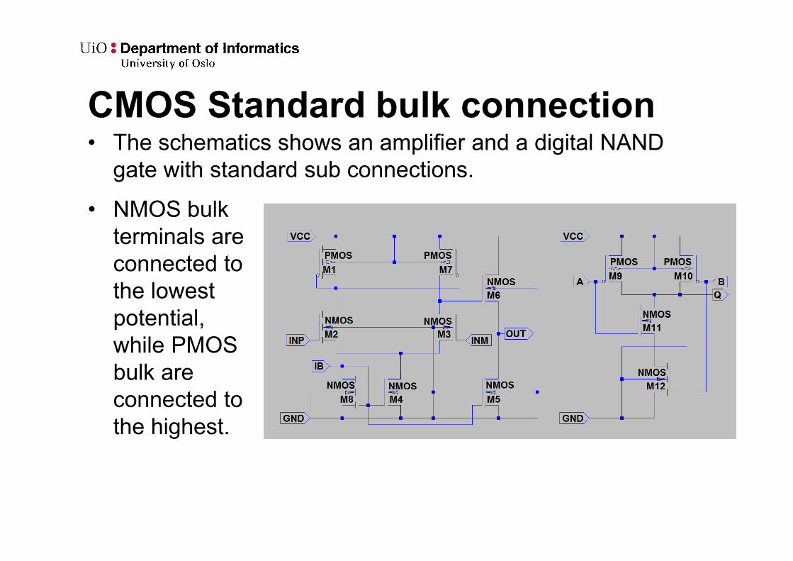
CMOS Standard bulk connection

• NMOS bulk terminals are connected to the lowest potential, while PMOS bulk are connected to the highest.

• The schematics shows an amplifier and a digital NAND gate with standard sub connections.

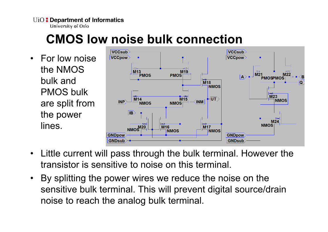
CMOS low noise bulk connection

• For low noise the NMOS bulk and PMOS bulk are split from the power lines.

• Little current will pass through the bulk terminal. However the transistor is sensitive to noise on this terminal.

• By splitting the power wires we reduce the noise on the sensitive bulk terminal. This will prevent digital source/drain noise to reach the analog bulk terminal.

LTspice: .NOISE analysis

• .NOISE is used to simulate component noise in the frequency-domain. The simulator includes by itself noise for all components in the schematic.

• Example: .NOISE V(out) V1 dec 200 1m 1G

– out: name of network node.

– V1: Name of source. May be voltage or current

– dec: Typ of sweep (decade, octave, linear or list)

– 200: Number of points per decade/octave

– 1m: Start frequency (1m=1milli Hz, 1Meg=1Mega Hz)

– 1G: Stop frequency

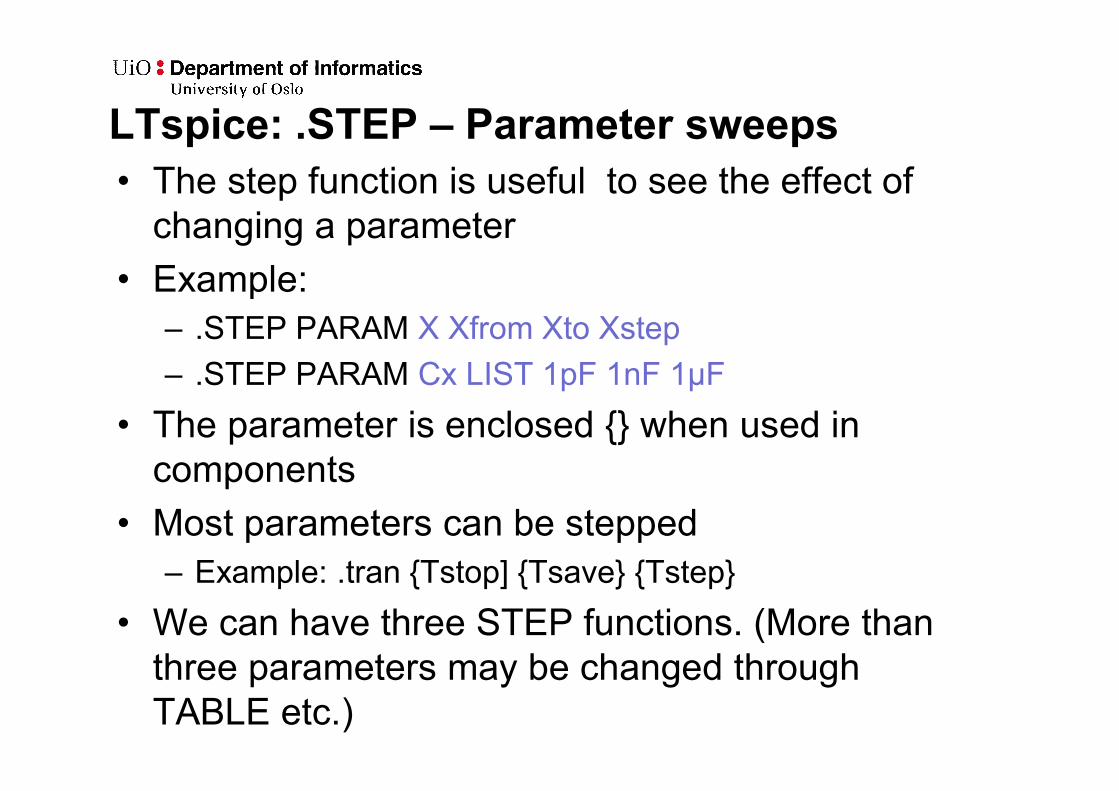
LTspice: .STEP – Parameter sweeps

• The step function is useful to see the effect of changing a parameter

• Example:

– .STEP PARAM X Xfrom Xto Xstep

– .STEP PARAM Cx LIST 1pF 1nF 1µF

• The parameter is enclosed {} when used in components

• Most parameters can be stepped

– Example: .tran {Tstop] {Tsave} {Tstep}

• We can have three STEP functions. (More than three parameters may be changed through TABLE etc.)

.STEP and TABLE

.STEP PARAM X LIST x0 x1 x2 x3

.PARAM Rx=table(X{index name},x0,y0,x1,y1,x2,y2,x3,y3)

Basically the index values (x0, x1, x2, x3) may have any numeric value. However if we would like to plot against step values we have chose depending on what we would like to have on our x-axis. Thus if we want a logarithmic scale we have to chose logarithmic index values.

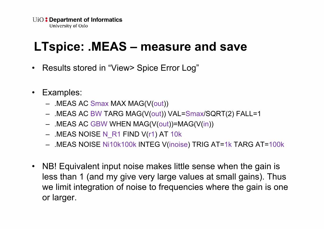
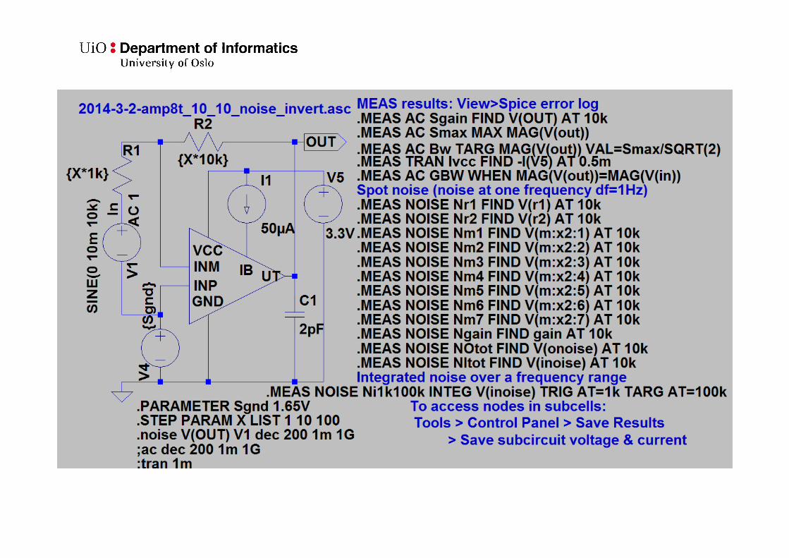
LTspice: .MEAS – measure and save

• Results stored in “View> Spice Error Log”

• Examples:– .MEAS AC Smax MAX MAG(V(out))

– .MEAS AC BW TARG MAG(V(out)) VAL=Smax/SQRT(2) FALL=1

– .MEAS AC GBW WHEN MAG(V(out))=MAG(V(in))

– .MEAS NOISE N_R1 FIND V(r1) AT 10k

– .MEAS NOISE Ni10k100k INTEG V(inoise) TRIG AT=1k TARG AT=100k

• NB! Equivalent input noise makes little sense when the gain is less than 1 (and my give very large values at small gains). Thus we limit integration of noise to frequencies where the gain is one or larger.

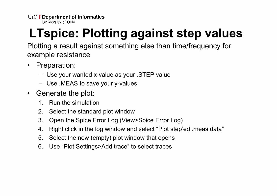
LTspice: Plotting against step valuesPlotting a result against something else than time/frequency for example resistance

• Preparation:– Use your wanted x-value as your .STEP value

– Use .MEAS to save your y-values

• Generate the plot:1. Run the simulation

2. Select the standard plot window

3. Open the Spice Error Log (View>Spice Error Log)

4. Right click in the log window and select “Plot step’ed .meas data”

5. Select the new (empty) plot window that opens

6. Use “Plot Settings>Add trace” to select traces