CENTRO DE ESTUDIOSMONETARIOS Y FINANCIEROS

www.cemfi.es

March 2017

working paper1710

Casado del Alisal 5, 28014 Madrid, Spain

Managers andProductivity Differences

Nezih GunerAndrii Parkhomenko

Gustavo Ventura

Gustavo.Ventura@asu.eduArizona State University

nezih.guner@cemfi.es

Keywords: Cross-country income differences, managers, distortions, management practices, size distribution, skill investment.

Nezih GunerCEMFI

Andrii ParkhomenkoUniversitat Autònoma de Barcelona & Barcelona parkhomenko.andrii@gmail.com

Gustavo Ventura

We document that for a group of high-income countries (i) mean earnings of managers tend to growfaster than for non managers over the life cycle; (ii) the earnings growth of managers relative to nonmanagers over the life cycle is positively correlated with output per worker. We interpret this evidence through the lens of an equilibrium life-cycle, span-of-control model where managers invest in theirskills. We parameterize this model with U.S. observations on managerial earnings, the size-distribution of plants and macroeconomic aggregates. We then quantify the relative importance ofexogenous productivity differences, and the size-dependent distortions emphasized in themisallocation literature. Our fi?ndings indicate that such distortions are critical to generate theobserved differences in the growth of relative managerial earnings across countries. Thus,observations on the relative earnings growth of managers become natural targets to discipline thelevel of distortions. Distortions that halve the growth of relative managerial earnings (a move from theU.S. to Italy in our data), lead to a reduction in managerial quality of 27% and to a reduction in outputof about 7% ? more than half of the observed gap between the U.S. and Italy. We ?find that cross-country variation in distortions accounts for about 42% of the cross-country variation in output perworker gap with the U.S.

CEMFI Working Paper No. 1710March 2017

Managers and Productivity Differences

Abstract

JEL Codes: E23, E24, J24, M11, O43, O47.

Acknowledgement

Guner acknowledges fi?nancial support from Spanish Ministry of Economy and Competitiveness,Grants ECO2011-28822 and ECO2014-54401-P, and from from the Generalitat of Catalonia, Grant2014SGR 803. Parkhomenko acknowledges fi?nancial from the FPI Severo Ochoa Scholarship fromMinistry of Economy and Competitiveness of Spain. We thank F. Buera and N. Roys for detailedcomments. We also thank workshop and conference participants at the 2016 ADEMU Workshop atEUI, UC-Berkeley, Cornell- Penn State Workshop, CREI, EEA-2015, Banco Central de Chile, ESEM2016, Federal Reserve Banks of Philadelphia and Richmond, IMF Macroeconomic Policy andIncome Inequality Workshop, NBER Summer Institute (Productivity and Macroeconomics), OhioState, Oslo, RIDGE-BCU Workshop, SED, Spanish Economic Association, 2015 Conference onEconomic Development (Montreal), and 2016 Western Conference on Misallocation and Productivityfor comments.

1 Introduction

Development accounting exercises conclude that productivity differences are central in un-

derstanding why some countries are richer than others (Klenow and Rodriguez-Clare, 1997;

Prescott, 1998; Hall and Jones, 1999; Caselli, 2005). What does determine cross country

productivity differences?

A growing literature emphasizes differences in management practices as a source of pro-

ductivity differences; see Bloom and Van Reenen (2011) and Bloom, Sadun and Van Reenen

(2016), among others. Management practices differ greatly, both across countries and across

firms within a given country, and better management practices are associated with better

performance (total factor productivity, profitability, survival etc.). U.S. firms on average

have the best management practices, and the quality of management declines rather sharply

as one moves to poorer countries.

In this paper, we present novel evidence on the earnings of managers and their relation

with output per worker. We first document that age-earnings profiles of managers differ

non trivially across countries. Using micro data for a set of high-income countries, we show

that earnings of managers grow much faster than the earnings of individuals who have non-

managerial occupations in most countries. In the United States, the earnings of managers

grow by about 75% during prime working ages (between ages 25-29 to 50-54), while the

earnings growth for non-managers is about 40%. This gap is weaker in other countries

in our sample. In Belgium, for instance, earnings growth of managers in prime working

years is about 65% whereas earnings growth of non-managers is similar to the U.S. On the

other extreme, we find that in Spain the earnings of non-managers grow more than those of

managers over the life-cycle.

We subsequently document that there is a strong positive relation between the relative

steepness of age-earnings profiles and GDP per worker: managerial earnings grow faster than

non-managerial earnings in countries with higher GDP per worker. The correlation coeffi cient

between the log of relative earnings and log-GDP per worker is 0.49, and stable across several

robustness checks on our data. Since better management practices and the GDP per worker

are positively correlated in the data, there is also a very strong positive relation between

the earnings growth of managers relative to the earnings growth of non managers and the

quality of management practices across countries. The relation between the relative steepness

2

of age-earnings profiles and GDP per worker remains robust when we control for individuals’

educational attainment, sector of employment and self-employment status. Furthermore,

these cross-country relations hold only when we look at the relative earnings growth of

managers vs. non-managers (workers). There is no systematic relation between GDP per

worker and the relative earnings growths of professionals (lawyers, engineers, doctors etc.)

vs. workers, self-employed vs. workers, or college-educated versus non-college educated.

It is, of course, an open question how to interpret differences in managerial practices

and quality across countries. In this paper, we offer a natural interpretation. Differences

in managerial quality emerge from differences in selection into management work, along the

lines of Lucas (1978), and differences in skill investments, as we allow for managerial abilities

to change over time as managers invest in their skills. Hence, we place incentives of managers

to invest in their skills and the resulting endogenous skill distribution of managers and their

incomes at the center of income and productivity differences across countries.

We study a span-of-control model with a life-cycle structure along a balanced growth

path. Every period, a large number of finitely-lived agents are born. These agents are

heterogeneous in terms of their initial endowment of managerial skills. The objective of each

agent is to maximize the lifetime utility from consumption. In the first period of their lives,

agents make an irreversible decision to be either workers or managers. If an agent chooses

to be a worker, her managerial skills are of no use and she earns the market wage in every

period until retirement. If an agent chooses to be a manager, she can use her managerial

skills to operate a plant by employing labor and capital to produce output and collect the

net proceeds (after paying labor and capital) as managerial income. Moreover, managers

invest resources in skill formation and, as a result, managerial skills grow over the life cycle.

This implies that a manager can grow the size of her production unit and managerial income

by investing a part of her current income in skill formation each period.

Skill investment decisions in the model reflect the costs (resources that have to be invested

rather than being consumed) and the benefits (the future rewards associated with being

endowed with better managerial skills). Since consumption goods are an input for skill

investments, a lower level of aggregate productivity results in lower incentives for managers

to invest in their skills. We assume that economy-wide productivity grows at a constant

rate. In this scenario, we show that the model economy exhibits a balanced growth path as

long as the managerial ability of successive generations grows at a constant rate.

3

A central component of our model is the complementarity between available skills and

investments in the production of new managerial skills. More skilled managers at a given

age invest more in their skills, which propagates and amplifies initial differences in skills over

the life cycle. This allows the model to endogenously generate a concentrated distribution of

managerial skills. As in equilibrium more skilled managers operate larger production units,

the model has the potential to account for the highly concentrated distribution of plant size

in data.

We calibrate the model to match a host of facts from the U.S. economy: macroeconomic

statistics, cross sectional features of establishment data as well as the age-earnings profiles

of managers. We assume for these purposes that the U.S. economy is relatively free of

distortions. We find that the model can indeed capture central features of the U.S. plant size

distribution, including the upper and lower tails. It also does an excellent job in generating

the age-earnings profiles of managers relative to non managers that we document from data.

We then proceed to introduce size-dependent distortions as in the literature on misalloca-

tion in economic development. We model size-dependent distortions as progressive taxes on

the output of a plant and do so via a simple parametric function, which was proposed origi-

nally by Benabou (2002). Size-dependent distortions have two effects in our setup. First, a

standard reallocation effect, as the enactment of distortions implies that capital and labor

services flow from distorted (large) to undistorted (small) production units. Second, a skill

accumulation effect, as distortions affect the incentives for skill accumulation and thus, the

overall distribution of managerial skills —which manifests itself in the distribution of plant

level productivity. Overall, the model provides us with a natural framework to study how

differences among countries in aggregate exogenous productivity and distortions can account

not only for differences in output per worker but also for differences in managerial quality,

size distribution of establishments and age-earnings profiles of managers. In particular, ob-

servations on the relative earnings growth of managers allows us to discipline the level of

distortions.

In consistency with the facts documented above, our model implies that lower levels

of economy-wide productivity result both in lower managerial ability as well as in flatter

relative age-earnings profiles. A 20% decline in aggregate productivity lowers investment in

skills by managers by nearly 48%, leading to a decline in the average quality of managers

of about 10%. With less investment, managerial incomes grow at a slower rate over the

4

life-cycle, generating the positive relation between output per worker and steepness of age-

income profiles that we observe in the data. Lower investment by managers magnifies the

effects of lower aggregate productivity, and output per worker declines by about 30%.

We then consider a menu of distortions and evaluate their effects on output, plant size,

notions of productivity, and age-earnings profiles of managers. When we introduce the size-

dependent distortions into the benchmark economy, we find substantial effects on output,

the size distribution of plants and the relative steepness of managerial earnings. We show

that such steepness is critically affected by distortions, and that distortions can eliminate all

differences in the earnings growth of managers to non-managers. We find that distortions

that halve the growth of relative managerial earnings (which would correspond to a move

from the U.S. to Italy in our data), lead to a reduction in output per worker of about 7%

—corresponding to more than half of the observed output gap between the U.S. and Italy.

As a result of both misallocation and skill investment effects, managerial quality declines

significantly by nearly 27%.

We find that these results are robust to the consideration of transitions between manage-

rial and non-managerial work over the life cycle. We do this in detail in Appendix III, where

we present an extension of the benchmark model with transitions between occupations.

We finally use the benchmark model to assess the combined effects of distortions and

exogenous variation in economy-wide productivity. For these purposes, we force the model

economy to reproduce jointly the level of output per worker in each country and the relative

earnings growth of managers. We do so by choosing economy-wide productivity levels and

the level of size dependency of distortions in each country to hit these two observations. We

find that distortions are critical in generating relative earnings growth across countries. As a

result, observations on relative earnings growth provide us with natural targets to discipline

the level of distortions. Once we are able to reproduce both the level of GDP per worker and

the relative earnings growth of managers within our model, we can assess the contribution of

economy-wide productivity and distortions to cross-country differences in output per worker.

To this end, we first allow economy-wide productivity to differ across countries and shut down

the distortion channel, and then do the reverse (i.e. we allow distortions to vary and shut

down differences in economy-wide productivity). We find that distortions alone account for

about 42% of variation in GDP per worker gap with the U.S. across countries, while the rest

of the variation is accounted for by differences in exogenous economy-wide productivity and

5

interaction effects. The level of distortions that reproduce the relative earnings growth of

managers in Italy (about half of the relative earnings growth in the US) are able to generate

about 43% of the observed output gap with the US.

1.1 Background

The current paper builds on recent literature that studies how misallocation of resources at

the micro level can lead to aggregate income and productivity differences; see Hopenhayn

(2014), Restuccia and Rogerson (2013) and Restuccia (2013) for recent reviews. Following

Guner, Ventura and Yi (2008) and Restuccia and Rogerson (2008), we focus in this paper

on implicit, size-dependent distortions as a source of misallocation.1 Unlike these papers, we

model explicitly how distortions and economy-wide productivity differences affect managers’

incentives to invest in their skills and generate an endogenous distribution of skills. As a

result, we show how data on relative earnings growth of managers can be used to infer the

degree of distortions within our model.

Our emphasis on age-earnings profiles of managers naturally links our paper to the empir-

ical literature on differences in management practices —see Bloom and Van Reenen (2011),

and Bloom, Lemos, Sadun, Scur and Van Reenen (2014) for recent surveys —as well as to the

recent development and trade literature that considers amplification effects of productivity

differences or distortions due to investments in skills and R&D. Examples of these papers

are Erosa, Koreshkova and Restuccia (2010), Rubini (2011), Atkeson and Burstein (2010,

2015), Gabler and Poschke (2013), Manuelli and Seshadri (2014), and Cubas, Ravikumar and

Ventura (2016), among others. Guvenen, Kuruscu and Ozkan (2014) study how progressive

taxation affects the incentives to accumulate general human capital and, as a result, output

for a group of high-income countries.

The importance of management and managerial quality for cross-country income differ-

ences have been emphasized by others before. Caselli and Gennaioli (2013) was possibly the

first paper that highlighted the importance of managers for cross-country income differences.

Caliendo and Rossi-Hansberg (2012) analyze how the internal organization of exporting firms

changes in response to trade liberalization and the ensuing effects on average productivity.

1Other papers have dealt with explicit policies in practice. Garcia-Santana and Pijoan-Mas (2014) studyexamples of size-dependent policies in India, while and Garicano, Lelarge and Van Reenen (2016) and Gourioand Roys ((2014) focus on France. Buera, Kaboski and Shi (2011), Cole, Greenwood and Sanchez (2016),and Midrigan and Xu (2014) focus on the role of financial frictions in leading to misallocation of resources.

6

Gennaioli, La Porta, Lopez-de-Silanes and Shleifer (2013) build a span-of-control model of

occupational choice with human capital externalities to study income differences across re-

gions. Recent work by Bhattacharya, Guner, and Ventura (2013), Roys and Seshadri (2014),

Akcigit, Alp and Peters (2016), and Alder (2016), among others, also study how managers

and their incentives matter for aggregate productivity and the size distribution of plants and

firms. Differently from these papers, we document novel facts on managerial earnings and

use these facts to discipline our model economy. Our emphasis on cross—country differences

in managerial earnings also relates our paper to Lagakos, Moll, Porzio, Qian and Schoell-

mann (2016), who study differences in experience-wage profiles across countries and show

that they are flatter in poorer countries. Similar to our findings, they highlight the fact that

experience-wage profiles are steeper in cognitive occupations relative to non-cognitive ones.

We focus on the relation between relative earnings growth of a particular group (managers)

and the GDP per capita across countries, and interpret this relation within a quantitative

model.

Our paper is also connected to work that documents cross-country differences in plant

and firm-level productivity and size. Hsieh and Klenow (2009), Bartelsman, Haltiwanger,

and Scarpetta (2013), Hsieh and Klenow (2014) and Garcia-Santana and Ramos (2015) are

examples of this line of work. Poschke (2014) builds a model of occupational choice with

skill-biased change in managerial technology —managers with better skills benefit more from

technological change —to account for cross-country differences in firm size distribution. Bento

and Restuccia (2016) document cross-country differences in plant size in manufacturing and

develop a model where distortions affect investments in plant-level productivity. In both

their model and ours, distortions are amplified by endogenous investment decisions. They

use this model to draw a mapping from plant size to aggregate productivity differences.

Finally, our paper is related to recent papers that emphasize the link between managerial

incentives, allocation of talent and income inequality. Celik (2016) studies how income

inequality can affect the allocation of talent between routine production and innovation in an

overlapping generations models in which agents can spend resources productively to enhance

their skills, or unproductively to create signals about their skills. More closely related to

our paper, Jones and Kim (2017) study a model in which heterogeneous entrepreneurs exert

effort to generate growth in their incomes and how such effort can create a Pareto-tail for

top incomes.

7

Our paper is organized as follows. Section 2 documents facts on age-earnings profiles for

a set of high income countries. Section 3 presents the model and the modeling of distortions.

Section 4 discusses the calibration of the benchmark model. Section 5 presents the findings

associated to the introduction of differences in exogenous economy-wide productivity and

size-dependent distortions. In section 6, we evaluate the importance of skill investments and

transitions between managerial and non-managerial work over the life cycle for our findings.

Section 7 quantifies the relative importance of distortions vis-a-vis exogenous productivity

differences in accounting for relative managerial earnings growth and output differences

across countries. Finally, section 8 concludes.

2 Managerial Earnings over the Life Cycle

In this section, we present age-earnings profiles for managers and non-managers for a group

of high-income countries. Panel data on income dynamics are available for a small set of

countries and even then, since individuals with managerial occupations constitute a small

group, it is not possible to construct age-earnings profiles for managers using panel data

sets. As a result, we conduct our analysis with large cross-sectional data sets pertaining to

different countries.

We use four data sources: The Integrated Public Use Microdata Series-USA (IPUMS-

USA), IPUMS-International, Luxembourg Income Study (LIS), and the European Union

Statistics on Income and Living Conditions (EU-SILC). IPUMS-International provides har-

monized Census data for a large set of countries. Only few international censuses, however,

contain information both on incomes and occupations. The LIS is another harmonized in-

ternational data set that contains cross-sectional individual level data on income and other

socioeconomic characteristics. Finally, the EU-SILC contains both cross-sectional and lon-

gitudinal microdata data for European Union countries on income, work, poverty, social

exclusion and living conditions.

Our final sample consists of 20 countries: Australia, Austria, Belgium, Canada, Denmark,

Finland, France, Germany, Iceland, Ireland, Israel, Italy, Luxembourg, Netherlands, Norway,

Spain, Sweden, Switzerland, the United Kingdom, and the United States. Table A1 in

Appendix I shows survey years, data sources, and the number of observations for each

country. Beyond data limitations, our focus on a set of high-income countries is motivated by

8

the fact that these countries are relatively similar in their aggregate levels of schooling and

hence, individuals are unlikely to differ much in terms of initial endowments of managerial

ability across countries. In developing countries, factors other than managerial abilities will

likely play a role in determining who is a manager and how much managers can invest in

their skills. Borrowing constraints, which we abstract from in our analysis, are much more

likely to be a factor in the allocation of talent in poorer countries. Likewise, selection into

managerial work as well as promotions are also more likely to be affected by family and

political connections.

We construct age-earnings profiles by estimating earnings equations as a function of age,

controlling for year effects and educational attainment. Specifically, for each country we

estimate the following regression:

ln yit = α + β1ait + β2a2it + γt + φ ei + εit, (1)

where yit is earnings and ait is age of individual i in year t. The coeffi cients β1 and β2 capture

the non-linear relationship between age and earnings, while γt represents year fixed-effects.

Finally, ei is an individual dummy variable capturing college education: it is equal to 1 if

the individual has a bachelor’s degree or higher, and zero otherwise. In this way we account

for the fact that countries differ in the educational attainment of their population and could

differ in the returns to education.2 We estimate this equation for individuals with managerial

and non-managerial occupations separately.

To estimate equation (1), we restrict the samples to ages 25 to 64, and group all ages

into eight 5-year age groups: 25-29, 30-34, ..., 60-64. Individuals are classified as managers

and non-managers based on their reported occupations. Table A2 in Appendix I documents

how managers are defined in different data sets. Whenever it is possible, we stick to the

occupational classification by the International Labor Organization.3 The sample is further

restricted to individuals who report positive earnings and work full time (at least 30 hours

2We could allow the coeffi cient on the college dummy to vary over time in order to capture the possibilitythat skill-biased technical change affected returns to college education. For most countries in our sample,however, we have relatively small number of panels for recent years (see Table A1 in Appendix I). As aresult, allowing the coeffi cient on the college dummy to vary over time does not change our estimates in anysignificant way.

3An individual is classified as a manager if his/her International Standard Classification of Occupations(ISCO-88) code is 11 ("Legislators, senior offi cials and managers"), 12 ("Corporate Managers"), or 13("General Managers"). We do not use the more recent ISCO-08, since most of our observations are datedearlier than 2008. Source: http://www.ilo.org/public/english/bureau/stat/isco/isco88/major.htm

9

per week). Earnings are defined as the sum of wage & salary income and self-employment

income. Most individuals in our samples earn either wages or self-employment income.

However, the samples contain a small number of managers and non-managers who report

positive amounts for both types of income.

Figure 1 reports age-earnings profiles for managers and non-managers for the US. Man-

agerial incomes grow by a factor of about 1.75 in prime working years —between ages 25-29

and 50-54 —whereas incomes of non-managers only rise by a factor of 1.4.4

Let the relative income growth, g be defined as

g = ln

(income manager, 50-54income manager, 25-29

income non manager, 50-54income non manager, 25-29

)(2)

Our key finding is the positive relationship between GDP per worker and the life cycle

growth of earnings of managers relative to the growth of non-managerial earnings.5 We

report this relationship in Figure 2. The slope of the fitted line is about 0.57, and the

correlation is 0.49. While some readers may view these findings with caution due to small

sample size, the relationship between log-GDP per worker and the steepness of managerial

age-earning profiles is remarkably strong and is statistically significant at the 5% significance

level.6 Consider countries along the fitted line in Figure 2. GDP per worker in Italy is about

11% lower than the GDP per worker in the U.S. This is associated with an almost 50%

decline in the relative earnings growth for managers (g declines from 22% to 11%). When we

go down to Sweden, GDP per worker declines by 23% from the U.S. level, while the relative

earnings growth declines by about 70% (g declines from 22% to 7%).

Since higher GDP per worker is also associated with better management practices, there

is also a very strong relation between the steepness of managerial age-earning profiles and

management practices. This relation is shown in Figure 3.7 In countries with better manage-

4While focusing on earnings growth during prime working years is natural, we also considered two alter-native specifications. First, relative earnings of managers compared to non managers may peak at differentages in different countries. In order to check whether our results are sensitive to this feature, we found theage bracket in which the relative earnings peak in each country and used this age bracket as the referenceage for computing the lifetime growth of relative income. Second, instead of using ages 50-54 as the referenceage bracket, we used 60-64, and looked at the earnings growth between 25-29 and 60-64. Our main resultsdo not change with these alternative specifications.

5We use the data on GDP per worker in year 2000 from Penn World Tables 7.1, Heston et al (2012)6We also checked for outliers that shifted the estimated coeffi cient by more than one standard deviation,

and we did not find any outliers with this particular metric.7The relation is significant at 10% significance level.

10

ment practices, such as the US or Germany, managers enjoy much higher relative earnings

growth compared to managers in countries with poor management practices, such as Italy.8

2.1 Robustness

We next perform multiple robustness checks regarding country size, the composition of the

sample and the regression equation. In all cases the relationship displayed in Figure 2 still

holds, and in some cases it becomes even stronger.9

Country Size We first run our benchmark regression under labor-force weights to

control for potential effects associated to country size. As Figure 4 shows, adjusting by

country size does not affect our results in any significant way. The magnitude of the slope

coeffi cient is now 0.49, with a correlation coeffi cient of 0.47. If we proceed even further, and

remove the richest but smallest country in the data, Luxembourg, the relationship is very

similar as Figure 5 shows.

Detailed Education and Sector Controls In our benchmark findings, we control

only for whether an individual, manager or non manager, has college education or not. We

now introduce more detailed education categories that are comparable across countries to

accommodate for potential heterogeneity in earnings profiles connected with educational

choices. For each country, we introduce dummies to capture whether an individual has (i)

complete tertiary education, (ii) incomplete tertiary but complete secondary education, or

(iii) any lower level of education, i.e. incomplete secondary, and complete or incomplete

primary education. Figure 6 displays the findings. As the figure shows, the relationship is

very similar to the benchmark one in Figure 2.

In addition, we control for sector of employment (both for managers and non-managers),

which might interact with the different levels of educational choices. Thus, on top of the

cases before, we add dummies if an individual works in the broad sectors of agriculture,

manufacturing or services. The results are displayed in Figure 7. As the figure shows, the

relationship becomes marginally stronger, with a slope coeffi cient of 0.59 and a correlation

8The data on management practices is from Bloom, Genakos, Sadun, and Van Reenen (2012), Table 2,and Bloom, Lemos, Sadun, Scur and Van Reenen (2014)

9The relations in Figures 4-10 are significant at 5% significance level.

11

of 0.51.10

The Role of Self Employment To what extent do our findings depend on the as-

sumption that some individuals have income from self employment? We answer this question

in two ways. First, we exclude the self-employed from the whole sample, i.e. both from

managers and non-managers, as well as only from the non-managers category. In the data,

self-employed individuals are either those who state that their main source of income is self-

employment, or the ones who have positive self-employment income and no wage and salary

income. Many self-employed, especially those who report a non-managerial occupation, have

both managerial and non-managerial duties and hence do not easily fit into our categoriza-

tion. Figures 8 and 9 show that our results are robust to exclusion of all self-employed and

self-employed non-managers.

Second, we narrow the definition of earnings to be wage and salary income only. Under

this restriction, the self-employed who earn positive wage and salary income — either as

managers or non-managers —are in the sample. However, their income from self-employment

is not counted as part of their earnings. Figure 10 illustrates that dropping self-employment

income from the notion of earnings only marginally changes our results. The slope coeffi cient

is now 0.61 and the correlation 0.47.

2.2 Are Managers Different?

The main result in this section (Figure 2) indicates that earnings of managers grow faster

relative to non-managers in richer countries. In the next section, we build a model economy

in which steeper age earnings profiles of managers emerge as the result of higher investments

that managers make to enhance their skills over the life-cycle in countries with either higher

aggregate productivity or lower distortions. There are of course other non-managerial occu-

pations/professions for which human capital investments over the life cycle arguably plays

a key role. Do we observe a similar relation between the relative steepness of age earnings

profiles and the GDP per worker for those other professions?

Figure 11 shows the findings when we replicate our exercise in Figure 2 for professionals

—lawyers, engineers, doctors, etc. — since individuals in this group are likely to be more

10Our main result also remains intact if we control for employment in the finance sector, as managerialearnings growth in this sector could arguably be much higher than in the rest of the economy.

12

similar to managers in terms of their incentives to invest in skills.11 We look at the earnings

growth for professionals (instead of managers) relative to the earnings growth of workers —

those who have non-professional, non-managerial occupations —versus GDP per worker. We

find that there is no positive relation between GDP per worker and the relative earnings

growth of professionals over their life-cycle. In Figure 12, we illustrate our findings when we

repeat the same exercise for self-employed individuals —who are often used in applied work

to capture the size of entrepreneurial activity in a country. Again, there is no systematic

relation between the earnings growth for self employed individuals relative to workers (those

who are not self-employed and have non-managerial occupations). Finally, we separate

individuals in two broad categories; those with college education — four years or more of

university education —and those without. Our results are illustrated in Figure 13. We find

in this case a small, near zero, relationship between relative earnings growth and output per

worker.

Overall, these results strongly suggest that forces that affect age earnings profiles of

managers relative to workers/non-managers are rather specific to the incentives they face,

and are unlikely to be due to factors that affect all individuals in the economy, such as

non-linear income taxation. We present below a parsimonious model able to capture these

key properties of the data.

3 Model

We develop a life-cycle, span-of-control model, where managers invest in their skills. Time is

discrete. Each period, a cohort of heterogeneous individuals that live for J periods are born.

Each individual maximizes the lifetime utility from consumption, so the life-time discounted

utility of an agent born at date t is given by

J∑j=1

βj−1 log(cj(t+ j − 1)), (3)

where β ∈ (0, 1) and cj(t) is the consumption of an age-j agent at date t.

Each agent is born with an initial endowment of managerial ability. We denote managerial

ability by z. We assume that initial (age-1) abilities of an agent born at date t are given by

11We define professionals as individuals who hold occupations in Group 2 in ISCO-88. Source:http://www.ilo.org/public/english/bureau/stat/isco/isco88/major.htm

13

z1(t) = Gz(t)z, and z is drawn from an exogenous distribution with cdf F (z) and density

f(z) on [0, zmax]. That is, individuals are heterogenous in initial managerial ability, and

abilities for newborns are shifted in each date by the factor Gz(t). We assume that Gz(t)

grows at the constant (gross) rate 1 + gz.

Each agent is also endowed with one unit of time which she supplies inelastically as a

manager or as a worker. In the very first period of their lives, agents must choose to be

either workers or managers. This decision is irreversible. If an individual chooses to be a

worker, her managerial effi ciency units are foregone, and she supplies one effi ciency unit of

labor at each age j. Retirement occurs exogenously at age JR. The decision problem of a

worker is to choose how much to consume and save every period.

If an individual chooses instead to be a manager, she has access to a technology to pro-

duce output, which requires managerial ability in conjunction with capital and labor services.

Hence, given factor prices, she decides how much labor and capital to employ every period.

In addition, in every period, a manager decides how much of his/her net income to allo-

cate towards current consumption, savings and investments in improving her/his managerial

skills. Retirement for managers also occurs exogenously at age JR.

We assume that each cohort is 1 + gN bigger than the previous one. These demographic

patterns are stationary so that age-j agents are a fraction µj of the population at any point

in time. The weights are normalized to add up to one, and obey the recursion, µj+1 =

µj/(1 + gN).

Technology Each manager has access to a span-of-control technology. A plant at date

t comprises of a manager with ability z along with labor and capital,

y(t) = A(t)z1−γ(kαn1−α

)γ,

where γ is the span-of-control parameter and αγ is the share of capital.12 The term A(t) is

productivity term that is common to all establishments, and given by A(t) = A GA(t), where

GA(t) grows at the (gross) rate 1 + gA. Thus, A controls the level of exogenous productivity.

Every manager can enhance her future skills by investing current income in skill accu-

mulation. The law of motion for managerial skills for a manager who is born at period t is

given by12In referring to production units, we use the terms establishment and plant interchangeably.

14

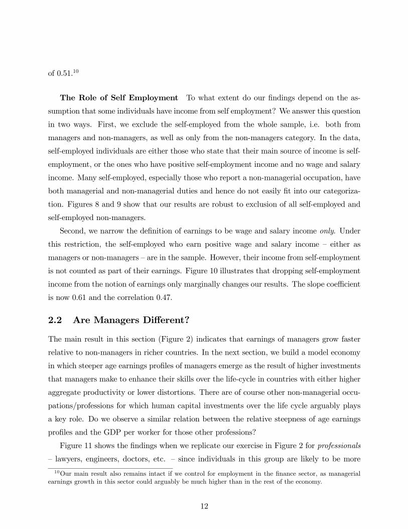
zj+1(t+ j) = (1− δz)zj(t+ j − 1) + g (zj(t+ j − 1), xj(t+ j − 1), j)

= (1− δz)zj(t+ j − 1) +B(j)zj(t+ j − 1)θ1xj(t+ j − 1)θ2 ,

where xj(t) is goods invested in skill accumulation by a manager of age j in period t. We

assume that θ1 ∈ (0, 1) and θ2 ∈ (0, 1). B(j) is the overall effi ciency of investment in skills at

age j. The skill accumulation technology described above satisfies three important properties,

of which the first two follow from the functional form and the last one is an assumption.

First, the technology shows complementarities between current ability and investments in

next period’s ability; i.e. gzx > 0. Second, g (z, 0, j) = 0. That is, investments are essential

to increase the stock of managerial skills. Finally, since θ2 < 1, there are diminishing returns

to skill investments, i.e. gxx < 0. Furthermore, we assume that B(j) = (1 − δθ)B(j − 1)

with B(1) = θ.

3.1 Decisions

Let factor prices be denoted by R(t) and w(t) for capital and labor services, respectively. Let

aj(t) denote assets at age j and date t that pay the risk-free rate of return r(t) = R(t)− δ.

Managers We assume that there are no borrowing constraints. As a result, factor

demands and per-period managerial income (profits) are age-independent, and only depend

on her ability z and factor prices. The income of a manager with ability z at date t is given

by

π(z, r, w,A, t) ≡ maxn,kA(t)z1−γ

(kαn1−α

)γ − w(t)n− (r(t) + δ)k.

Factor demands are given by

k(z, r, w,A, t) = (A(t)(1− α)γ)1

1−γ

(α

1− α

) 1−γ(1−α)1−γ

(1

r(t) + δ

) 1−γ(1−α)1−γ

(1

w(t)

) γ(1−α)1−γ

z,

(4)

and

n(z, r, w,A, t) = (A(t)(1− α)γ)1

1−γ

(α

1− α

) αγ1−γ(

1

r(t) + δ

) αγ1−γ(

1

w(t)

) 1−αγ1−γ

z. (5)

15

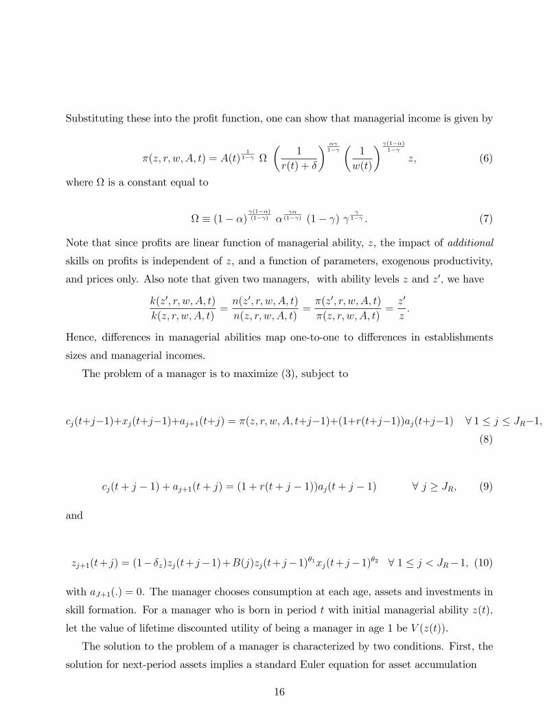
Substituting these into the profit function, one can show that managerial income is given by

π(z, r, w,A, t) = A(t)1

1−γ Ω

(1

r(t) + δ

) αγ1−γ(

1

w(t)

) γ(1−α)1−γ

z, (6)

where Ω is a constant equal to

Ω ≡ (1− α)γ(1−α)(1−γ) α

γα(1−γ) (1− γ) γ

γ1−γ . (7)

Note that since profits are linear function of managerial ability, z, the impact of additional

skills on profits is independent of z, and a function of parameters, exogenous productivity,

and prices only. Also note that given two managers, with ability levels z and z′, we have

k(z′, r, w,A, t)

k(z, r, w,A, t)=n(z′, r, w,A, t)

n(z, r, w,A, t)=π(z′, r, w,A, t)

π(z, r, w,A, t)=z′

z.

Hence, differences in managerial abilities map one-to-one to differences in establishments

sizes and managerial incomes.

The problem of a manager is to maximize (3), subject to

cj(t+j−1)+xj(t+j−1)+aj+1(t+j) = π(z, r, w,A, t+j−1)+(1+r(t+j−1))aj(t+j−1) ∀ 1 ≤ j ≤ JR−1,

(8)

cj(t+ j − 1) + aj+1(t+ j) = (1 + r(t+ j − 1))aj(t+ j − 1) ∀ j ≥ JR, (9)

and

zj+1(t+ j) = (1−δz)zj(t+ j−1)+B(j)zj(t+ j−1)θ1xj(t+ j−1)θ2 ∀ 1 ≤ j < JR−1, (10)

with aJ+1(.) = 0. The manager chooses consumption at each age, assets and investments in

skill formation. For a manager who is born in period t with initial managerial ability z(t),

let the value of lifetime discounted utility of being a manager in age 1 be V (z(t)).

The solution to the problem of a manager is characterized by two conditions. First, the

solution for next-period assets implies a standard Euler equation for asset accumulation

16

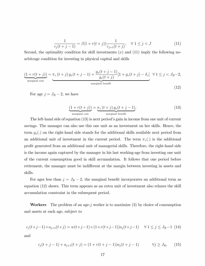
1

cj(t+ j − 1)= β(1 + r(t+ j))

1

cj+1(t+ j), ∀ 1 ≤ j < J (11)

Second, the optimality condition for skill investments (x) and (11) imply the following no-

arbitrage condition for investing in physical capital and skills

(1 + r(t+ j))︸ ︷︷ ︸marginal cost

= πz (t+ j) gx(t+ j − 1) +gx(t+ j − 1)

gx(t+ j)[1 + gz(t+ j)− δz]︸ ︷︷ ︸

marginal benefit

∀ 1 ≤ j < JR−2,

(12)

For age j = JR − 2, we have

(1 + r(t+ j))︸ ︷︷ ︸marginal cost

= πz (t+ j) gx(t+ j − 1)︸ ︷︷ ︸marginal benefit

, (13)

The left-hand side of equation (13) is next period’s gain in income from one unit of current

savings. The manager can also use this one unit as an investment on her skills. Hence, the

term gx(.) on the right-hand side stands for the additional skills available next period from

an additional unit of investment in the current period. The term πz(.) is the additional

profit generated from an additional unit of managerial skills. Therefore, the right-hand side

is the income again captured by the manager in his last working-age from investing one unit

of the current consumption good in skill accumulation. It follows that one period before

retirement, the manager must be indifferent at the margin between investing in assets and

skills.

For ages less than j = JR − 2, the marginal benefit incorporates an additional term as

equation (12) shows. This term appears as an extra unit of investment also relaxes the skill

accumulation constraint in the subsequent period.

Workers The problem of an age-j worker is to maximize (3) by choice of consumption

and assets at each age, subject to

cj(t+j−1)+aj+1(t+j) = w(t+j−1)+(1+r(t+j−1))aj(t+j−1) ∀ 1 ≤ j ≤ JR−1 (14)

and

cj(t+ j − 1) + aj+1(t+ j) = (1 + r(t+ j − 1))aj(t+ j − 1) ∀j ≥ JR, (15)

17

with aJ+1(.) = 0. Like managers, workers can borrow and lend without any constraint as

long as they do not die with negative assets. For an individual born period t, let the life-time

discounted utility of being a worker at age 1 be given by W (t).

Occupational Choice Let z∗(t) be the ability level at which a 1-year old agent is

indifferent between being a manager and a worker. This threshold level of z is given by (as

agents are born with no assets)

V (z∗(t)) = W (t). (16)

Given all the assumptions made, V is a continuous and a strictly increasing function of z.

Therefore, (16) has a well-defined solution, z∗(t), for all t.

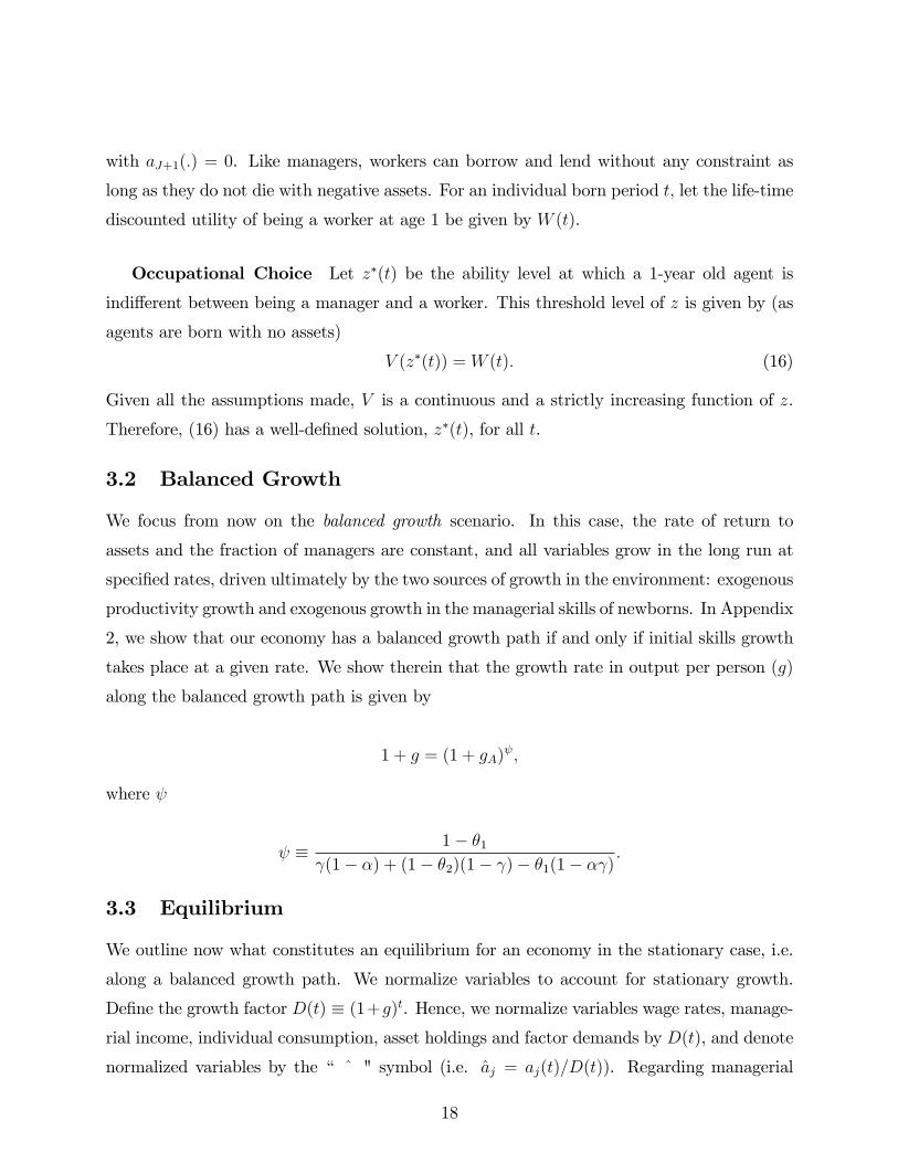
3.2 Balanced Growth

We focus from now on the balanced growth scenario. In this case, the rate of return to

assets and the fraction of managers are constant, and all variables grow in the long run at

specified rates, driven ultimately by the two sources of growth in the environment: exogenous

productivity growth and exogenous growth in the managerial skills of newborns. In Appendix

2, we show that our economy has a balanced growth path if and only if initial skills growth

takes place at a given rate. We show therein that the growth rate in output per person (g)

along the balanced growth path is given by

1 + g = (1 + gA)ψ,

where ψ

ψ ≡ 1− θ1γ(1− α) + (1− θ2)(1− γ)− θ1(1− αγ)

.

3.3 Equilibrium

We outline now what constitutes an equilibrium for an economy in the stationary case, i.e.

along a balanced growth path. We normalize variables to account for stationary growth.

Define the growth factor D(t) ≡ (1+g)t. Hence, we normalize variables wage rates, manage-

rial income, individual consumption, asset holdings and factor demands by D(t), and denote

normalized variables by the “ ˆ " symbol (i.e. aj = aj(t)/D(t)). Regarding managerial

18

abilities, recall that managerial ability levels of members of each new cohort are given by

z1(t) = z(t)z, with a common component that grows over time at the rate gz, and a random

draw, z, distributed with cdf F (z) and density f(z) on [0, zmax]. Hence, the normalized com-

ponent is simply z for each individual. After the age-1, and given the stationary threshold

value z∗, the distribution of managerial abilities is endogenous as it depends on investment

decisions of managers over their life-cycle.

Let managerial abilities take values in set Z = [z∗, z] with the endogenous upper bound

z. Similarly, let A = [0, a] denote the possible asset levels. Let ψj(a, z) be the mass of age-j

agents with assets a and skill level z. Given ψj(a, z), let

fj(z) =

∫ψj(a, z)da,

be the skill distribution for age-j agents. Note that f1(z) = f(z) by construction.

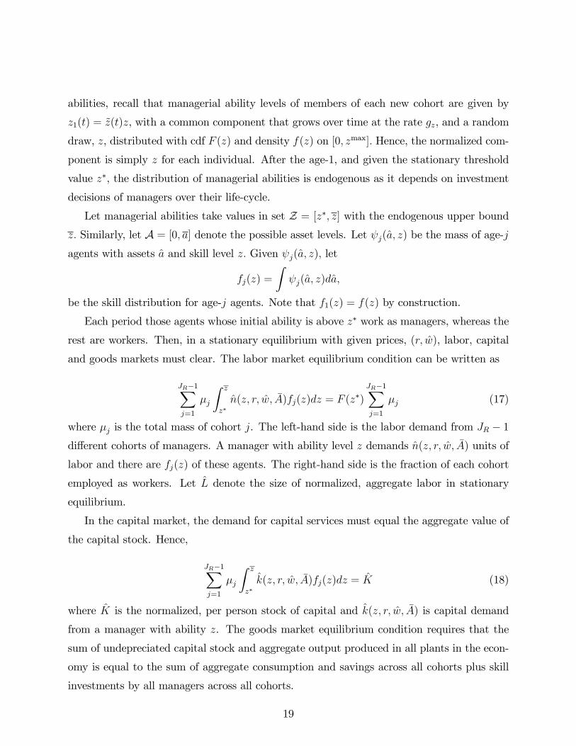
Each period those agents whose initial ability is above z∗ work as managers, whereas the

rest are workers. Then, in a stationary equilibrium with given prices, (r, w), labor, capital

and goods markets must clear. The labor market equilibrium condition can be written as

JR−1∑j=1

µj

∫ z

z∗n(z, r, w, A)fj(z)dz = F (z∗)

JR−1∑j=1

µj (17)

where µj is the total mass of cohort j. The left-hand side is the labor demand from JR − 1

different cohorts of managers. A manager with ability level z demands n(z, r, w, A) units of

labor and there are fj(z) of these agents. The right-hand side is the fraction of each cohort

employed as workers. Let L denote the size of normalized, aggregate labor in stationary

equilibrium.

In the capital market, the demand for capital services must equal the aggregate value of

the capital stock. Hence,

JR−1∑j=1

µj

∫ z

z∗k(z, r, w, A)fj(z)dz = K (18)

where K is the normalized, per person stock of capital and k(z, r, w, A) is capital demand

from a manager with ability z. The goods market equilibrium condition requires that the

sum of undepreciated capital stock and aggregate output produced in all plants in the econ-

omy is equal to the sum of aggregate consumption and savings across all cohorts plus skill

investments by all managers across all cohorts.

19

Discussion We now discuss a few properties of the model economy that are of im-

portance for our subsequent analysis. First, it is worth noting that managerial investments

are essential for the model to reproduce the facts on managerial earnings documented in

section 2. In the absence of investments, initial managerial ability depreciates and manage-

rial earnings would decline over the life cycle. This stands in contrast with the evidence

documented for the United States and other countries, where earnings of managers relative

to non managers grow substantially with age.

Second, our environment offers a natural notion of aggregate managerial quality, or total

managerial skills per manager, Z. Formally,

Z ≡∑JR−1

j=1 µj∫ zz∗ zfj(z)dz

M, (19)

where M is the number of managers in equilibrium. Hence, changes in managerial quality

in response to changes in the environment are determined by changes in the number of

managers (i.e. changes in z∗), as well as by changes in the distribution of skills. That is,

changes in the incentives to accumulate managerial skills will naturally induce changes in

managerial quality. Even if the threshold z∗ is unchanged in response to a change in the

environment, the mass of individuals at each level of managerial ability over the life cycle

will change as individuals optimally adjust their skill accumulation plans.

Finally, our model of production at heterogenous units aggregates into an production

function. It is possible to show that aggregate output can be written as

Y = A Z1−γ M1−γ KγαLγ(1−α) (20)

As we discuss in next sections, changes in occupational decisions across steady-state equi-

libria affect output in different ways. On the one hand, a reduction in z∗ raises the number

of managers but reduces the size of aggregate labor in equation (20). On the other hand, a

reduction in z∗ reduces the magnitude of managerial quality as defined above since marginal

managers are less able than inframarginal ones. As we show next, the resulting managerial

quality changes can be quantitatively large in response to policy-induced occupational shifts.

20

3.4 Size-Dependent Distortions

Consider now the stationary environment in which managers face distortions to operate

production plants. We model these distortions as size-dependent output taxes. In particular,

we assume an establishment with output y faces an average tax rate T (y) = 1− λy−τ . Thistax function, initially proposed by Benabou (2002), has a very intuitive interpretation: when

τ = 0, distortions are the same for all establishments and they all face an output tax of

(1− λ). For τ > 0, the distortions are size-dependent, i.e. larger establishments face higher

distortions than smaller ones. Hence, τ controls how dependent on size the distortions are.13

With distortions, profits are given by

π(z, r, w, A) = maxn,kλA1−τz(1−γ)(1−τ)

(kαn1−α

)γ(1−τ)︸ ︷︷ ︸after-tax output

− wn− (r + δ)k

From the first order conditions, the factor demands are now given by

n(z, r, w, A) =[λA1−τγ(1− α)(1− τ)

] 11−γ(1−τ) × (21)

×(

1

r + δ

) γα(1−τ)1−γ(1−τ)

(α

1− α

) γα(1−τ)1−γ(1−τ)

(1

w

) 1−γα(1−τ)1−γ(1−τ)

z(1−γ)(1−τ)1−γ(1−τ) ,

and

k(z, r, w, A) =[λA1−τγ(1− α)(1− τ)

] 11−γ(1−τ) × (22)

×(

1

r + δ

) 1−γ(1−α)(1−τ)1−γ(1−τ)

(α

1− α

) 1−γ(1−α)(1−τ)1−γ(1−τ)

(1

w

) γ(1−α)(1−τ)1−γ(1−τ)

z(1−γ)(1−τ)1−γ(1−τ) .

Using the factor demands 21 and 22, we can write the profit function as

π(z, r, w, A) =(λA1−τ

) 11−γ(1−τ) Ω

(1

r + δ

) αγ1−γ(

1

w

) γ(1−α)1−γ

z(1−γ)(1−τ)1−γ(1−τ) (23)

where

Ω ≡ (1− γ(1− τ))αγα(1−τ)1−γ(1−τ) (1− α)

γ(1−α)(1−τ)1−γ(1−τ) (γ (1− τ))

γ(1−τ)1−γ(1−τ) .

13This specification has been recently used by Bauer and Rodriguez-Mora (2014) and Bento and Restuc-cia (2016) in the development literature. In a public-finance context, this specification has been used byHeathcote, Storesletten and Violante (2016) and Guner, Lopez-Daneri and Ventura (2016), among others,to analyze the effects of income tax progressivity.

21

Note that for any z and z′, we now have

k(z′, r, w, A)

k(z, r, w, A)=n(z′, r, w, A)

n(z, r, w, A)=π(z′, r, w, A)

π(z, r, w, A)=

(z′

z

) (1−γ)(1−τ)1−γ(1−τ)

,

where(1− γ)(1− τ)

1− γ(1− τ)< 1,

as long as τ > 0. That is, for a given distribution of managerial abilities, size-dependent

distortions produce a more compressed size distribution of establishments and managerial

incomes.

Similarly, for any z and z′ the optimal skill investment is now characterized by

x′jxj

=

(z′jzj

)(θ1− τ1−γ(1−τ))

11−θ2

.

It is easy to show that the exponent in the expression is decreasing with respect to the para-

meter τ governing size dependency. Hence, size-dependent distortions also reduce incentives

of higher-ability managers to invest in their skills.

4 Parameter Values

We assume that the U.S. economy is free of distortions, and calibrate the benchmark model

parameters to match aggregate and plant-size moments as well as moments on managerial

incomes from the U.S. data. In particular, we force our economy to reproduce the earnings

of managers relative to non-managers over the life cycle estimated in section 2. We divide

our discussion of parameter choices between parameters that are set directly from data and

those that are inferred so the model reproduce data moments in equilibrium.

Data and Parametric Assumptions For observations on the U.S. plant sizes, we

use the 2004 U.S. Economic Census. The average plant size is about 17.9 employees, and

the distribution of employment across plants is quite skewed. About 72.5% of plants in the

economy employ less than 10 workers, but account for only 15% of the total employment.

On the other hand, less than 2.7% of plants employ more than 100 employees but account

for about 46% of total employment. From our findings in section 2, managerial incomes

(relative to non-managers) grow by about 18% between ages 25-29 to 40-44 —g value equal

to 16.8% —and by about 25% by ages 60-64 —g value equal to 22.1%.

22

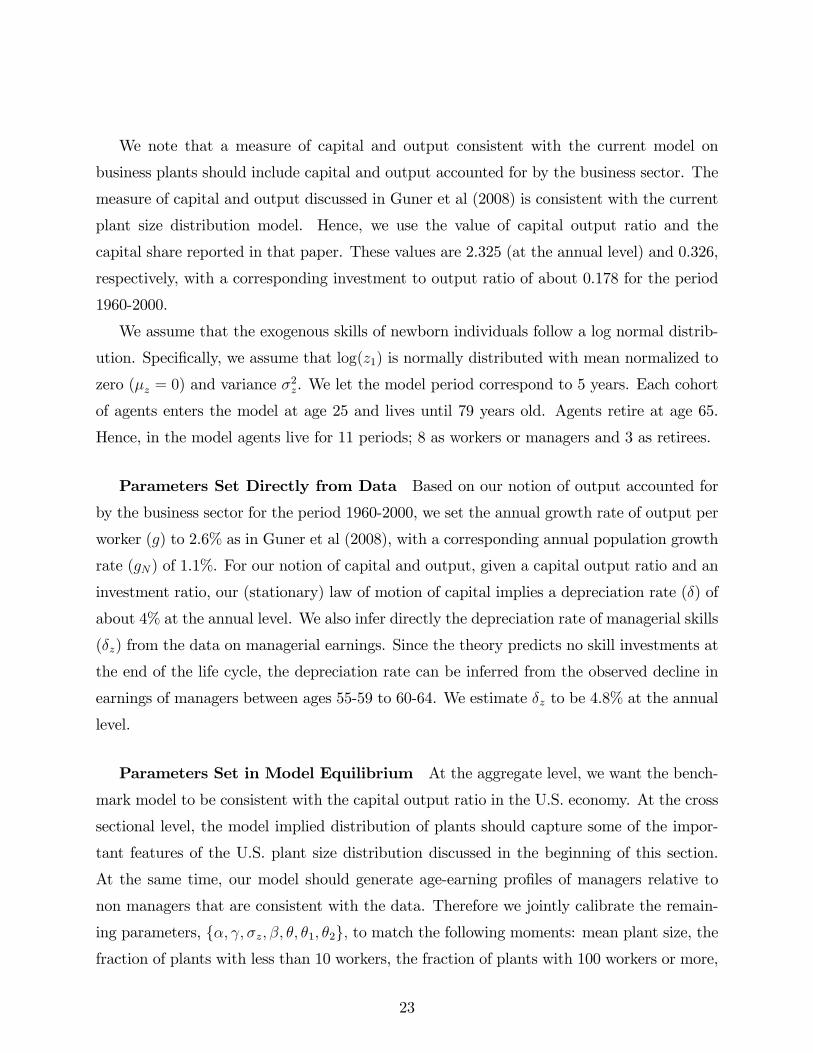
We note that a measure of capital and output consistent with the current model on

business plants should include capital and output accounted for by the business sector. The

measure of capital and output discussed in Guner et al (2008) is consistent with the current

plant size distribution model. Hence, we use the value of capital output ratio and the

capital share reported in that paper. These values are 2.325 (at the annual level) and 0.326,

respectively, with a corresponding investment to output ratio of about 0.178 for the period

1960-2000.

We assume that the exogenous skills of newborn individuals follow a log normal distrib-

ution. Specifically, we assume that log(z1) is normally distributed with mean normalized to

zero (µz = 0) and variance σ2z. We let the model period correspond to 5 years. Each cohort

of agents enters the model at age 25 and lives until 79 years old. Agents retire at age 65.

Hence, in the model agents live for 11 periods; 8 as workers or managers and 3 as retirees.

Parameters Set Directly from Data Based on our notion of output accounted for

by the business sector for the period 1960-2000, we set the annual growth rate of output per

worker (g) to 2.6% as in Guner et al (2008), with a corresponding annual population growth

rate (gN) of 1.1%. For our notion of capital and output, given a capital output ratio and an

investment ratio, our (stationary) law of motion of capital implies a depreciation rate (δ) of

about 4% at the annual level. We also infer directly the depreciation rate of managerial skills

(δz) from the data on managerial earnings. Since the theory predicts no skill investments at

the end of the life cycle, the depreciation rate can be inferred from the observed decline in

earnings of managers between ages 55-59 to 60-64. We estimate δz to be 4.8% at the annual

level.

Parameters Set in Model Equilibrium At the aggregate level, we want the bench-

mark model to be consistent with the capital output ratio in the U.S. economy. At the cross

sectional level, the model implied distribution of plants should capture some of the impor-

tant features of the U.S. plant size distribution discussed in the beginning of this section.

At the same time, our model should generate age-earning profiles of managers relative to

non managers that are consistent with the data. Therefore we jointly calibrate the remain-

ing parameters, α, γ, σz, β, θ, θ1, θ2, to match the following moments: mean plant size, thefraction of plants with less than 10 workers, the fraction of plants with 100 workers or more,

23

the fraction of the labor force employed in plants with 100 or more employees, the growth

of managerial incomes relative to those of non-managers between ages 25-29 and 40-44, the

growth of managerial incomes relative to those of non-managers between ages 25-29 to 60-64,

and the aggregate capital-output ratio.14 Note that since the capital share in the model is

given by γα, and since this value has to be equal to the data counterpart (0.326), a calibrated

value for γ determines α as well.

The resulting parameter values are displayed in Table 1. Table 2 shows the targeted

moments together with their model counterparts as well as the entire plant size distribution.

Skill Investments In our calibration, the fraction of resources that are invested in

skill accumulation is about 0.9% of GDP. Despite the relatively small fraction of resources

devoted to the improvement of managerial skills, the incomes of managers grow significantly

with age in line with data. Figure 14 shows that the earnings of managers relative to non

managers in the model are in conformity with the data. It is important to emphasize that

managerial skill investments play a central role in the growth of earnings. If we halve the

value of the parameter θ2 that governs the incentives to invest goods in skill formation, we

find that resources invested in skill accumulation drop to about 0.6% of output and the

earnings growth of managers relative to non managers between ages 25-29 and 60-64 (g)

drops from the benchmark value of 22% to 10%.

It is also important to mention that the benchmark model is able to replicate the proper-

ties of the entire plant size distribution fairly well, as demonstrated in Table 2. In particular,

the model is able to generate the concentration of employment in very large plants. Again,

skill accumulation plays an important role in this case. We calculate that if we give managers

the skills they are born with for their entire life cycle (i.e. skill formation is not allowed), the

mean plant size drops from 17.7 to about 15.7, and the share of employment accounted for

by large plants (100 employees and higher) drops from 46% to 37.8%. In similar fashion, if

14Within our framework, since each plant has one manager, targeting mean plant size determines a fractionof managers. Finding an empirical target for the fraction of managers (workers) is not straightforward. Incontrast to he model economy, each plant in the data might have several managers in different layers andhierarchies. In the benchmark economy, about 5.3% of population are managers, which would be the fractionof managers if we assume that each plant is run by a single manager in the data. In the benchmark dataused in Section 2 under the classification for cross-country purposes, about 10% of workforce are managersin the United States. Further restrictions on who is a manager in the data makes the fraction of managerssmaller, and easily less than the value implied by our model.

24

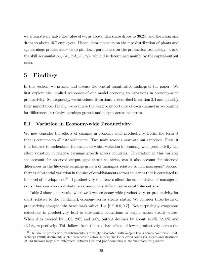
we alternatively halve the value of θ2, as above, this share drops to 36.2% and the mean size

drops to about 15.7 employees. Hence, data moments on the size distribution of plants and

age-earnings profiles allow us to pin down parameters on the production technology, γ, and

the skill accumulation, σz, θ, δz, θ1, θ2, while β is determined mainly by the capital-outputratio.

5 Findings

In this section, we present and discuss the central quantitative findings of the paper. We

first explore the implied responses of our model economy to variations in economy-wide

productivity. Subsequently, we introduce distortions as described in section 3.4 and quantify

their importance. Finally, we evaluate the relative importance of each channel in accounting

for differences in relative earnings growth and output across countries.

5.1 Variation in Economy-wide Productivity

We now consider the effects of changes in economy-wide productivity levels; the term A

that is common to all establishments. Two main reasons motivate our exercises. First, it

is of interest to understand the extent to which variation in economy-wide productivity can

affect variation in relative earnings growth across countries. If variation in this variable

can account for observed output gaps across countries, can it also account for observed

differences in the life-cycle earnings growth of managers relative to non managers? Second,

there is substantial variation in the size of establishments across countries that is correlated to

the level of development.15 If productivity differences affect the accumulation of managerial

skills, they can also contribute to cross-country differences in establishment size.

Table 3 shows our results when we lower economy-wide productivity, or productivity for

short, relative to the benchmark economy across steady states. We consider three levels of

productivity alongside the benchmark value; A = 0.9, 0.8, 0.7. Not surprisingly, exogenousreductions in productivity lead to substantial reductions in output across steady states.

When A is lowered by 10%, 20% and 30%, output declines by about 15.5%, 29.8% and

43.1%, respectively. This follows from the standard effects of lower productivity across the

15The size of production establishments is strongly associated with output levels across countries. Bhat-tacharya (2010) documents such differences in establishment size for selected countries. Bento and Restuccia(2016) uncover large size differences between rich and poor countries in the manufacturing sector.

25

board, in conjunction with the lower accumulation of managerial skills over the life cycle

emphasized here. In this regard, Table 3 shows that investment in managerial skills drops

from about 0.9% of output to about 0.6% when economy-wide productivity drops by 30%.

As a result of lower investment in managerial skills, relative age-earnings profiles become

flatter as Table 3 demonstrates. A reduction in economy-wide productivity of 20% trans-

lates into a reduction of more than half in the earnings growth of managers relative to non

managers. Relative earnings growth can even turn negative for low values of economy-wide

productivity. Therefore, the model has the potential to generate the positive relation be-

tween GDP per worker and the steepness of age-earnings profiles documented in section 2

(see Figure 2).

It is worth relating these results to properties of standard span-of-control models. First,

managerial skills are simply endowments in models of that class. Thus, in a life-cycle context,

such models cannot account for the relative earnings facts documented in section 2. Second,

the same forces that lead to changes in the steepness of relative managerial profiles lead

also to equilibrium changes in plant size. Changes in exogenous productivity, as modeled

here, do not generate size differences in a growth model with a Lucas (1978) span-of-control

technology, as changing A has no effect on occupational decisions.16 The consequences of

changing aggregate productivity, however, are different in the current setup. As productivity

drops, both wage rates and managerial rents drop as in the standard span-of-control model.

But a productivity drop also reduces the marginal benefit associated to an extra unit of

income invested in skill accumulation (see equations 12 and 13). As a result, managerial

skills become overall lower, which translates into further reductions in labor demand and

therefore, on the wage rate. The net result is a reduction in the value of becoming a worker

relative to a manager at the start of life, which leads in turn to an increase in the number of

managers. Quantitatively, however, these size effects are moderate as Table 3 demonstrates.

Finally, Table 3 shows that aggregate managerial quality drops alongside reductions in

economy-wide productivity: a reduction in A of 30% translates into a reduction in managerial

quality of more than 15%. Again, this occurs due to the presence of investments in managerial

skills. Lower managerial quality follows from the (small) increase in the number of managers

across steady states, in conjunction with lower investments in managerial skills in response

16This requires a Cobb-Douglas specification as we assume in this paper.

26

to a reduction in economy-wide productivity —see equation (19).

Output and Earnings Growth Differences Given the results in Table 3, it is natural

to ask the extent to which the model can reproduce the relation between GDP per worker

and the relative earnings growth for managers that we observe in the data. To this end,

for each of the countries in our data, we select a value of A such that our model economy

reproduces GDP per worker of that country relative to the U.S. We keep all other parameters

fixed at their benchmark values.

We find that the model predicts a weaker relationship between output and the relative

earnings growth of managers over the life cycle than it is observed in the data. While in the

data the slope coeffi cient between these variables is about 0.57, our model predicts a value

of about 0.39. In other words, there is more variation in relative earnings growth in the data

that what our model predicts exclusively via changes in economy-wide productivity. Output

changes driven by changes in economy-wide productivity are not accompanied, however, by

corresponding reductions in relative earnings growth as observed in the data. As a result,

the variance in g implied by the model is just about 11% of the variance of this variable in

the data.

5.2 Size-Dependent Distortions

We now study the quantitative role of size-dependent distortions via the implicit tax function

T (y) = 1 − λy−τ , as explained in section 3.4. The key in this formulation is the curvatureparameter τ governing the degree of size dependency; if τ > 0, the plants with higher output

levels face higher marginal and average rates, while if τ = 0, implicit taxes are the same for

all, regardless of the level of output.

We evaluate the consequences across steady states of an array of values for the parameter

τ in Table 4, under λ = 1. For each value of τ , Table 4 also reports the implied distortion

wedge, measured as the take home rate, 1− T (y), evaluated at 5 times the mean output.

As Table 4 demonstrates, the effects of size-dependent distortions can be dramatic on some

variables. Introducing size-dependent distortions leads to a reduction in output across steady

states, an increase in the number of managers (reduction of plant size), and to a reallocation

of output and employment to smaller production units. In the context of the current setup,

these effects are concomitant with less investment in managerial skills and thus, with less

27

steep age-earnings profiles of managers relative to non-managers. This occurs as with the

introduction of distortions that are size dependent, large establishments reduce their demand

for capital and labor services relatively more than smaller ones, leading to a reduction in the

wage rate. This prompts the emergence of smaller production units, as individuals with low

initial managerial ability become managers. This is the mechanism highlighted in Guner et

al (2008) and others. In addition, investment in skills decline in the current setup reinforcing

the equilibrium effects on output, size and managerial quality.

The Quantitative Importance of Distortions How large are the distortions im-

posed by different levels of τ? To answer this question, we calculate the distortions borne

by large plants at high multiples of mean output levels relative to those at mean output.17

From this perspective, we find that distortions do not increase too much with output. For

instance, the distorting factor at five times mean output amounts to 0.97, 0.94, and 0.91,

for values of τ of 0.02, 0.04 and 0.06, respectively. That is, in all cases the distorting factors

differ by less than ten percentage points.

Quantitatively, raising size dependency from zero to τ = 0.02 leads to a reduction in

output of about 7.1%, a reduction in mean size from 17.7 to 13.2 employees, and to a sizable

reduction in managerial quality of about 26.7%. The effect on the relative earnings growth

of managers is substantial, with a reduction in the slope coeffi cient (g) to less than half

the benchmark value. Indeed, as Table 4 shows, it is possible to eliminate all growth in

relative managerial earnings over the life cycle! A value of τ = 0.06 leads to a negative

slope coeffi cient. Such change is accompanied by a drop in output of about 18.7%, and by a

drastic reduction in managerial quality of about 54.4%.

It is worth noting that the concentration of employment at large establishments drops

significantly with distortions. About 46% of employment is accounted for by plants with

100 employees or more in the benchmark economy. This figure drops sharply as the size

dependency of distortions becomes more important. At τ = 0.02, the share of employment

in large establishments is 34% while at τ = 0.06, this variable falls to less than half of its

benchmark value. The behavior of the employment at large establishments in response to

17Specifically, we calculate the ratio of one minus the marginal rate on plants at q times mean outputrelative to mean output. Since one minus the marginal tax rate amounts to (1−τ)λy−τ , this ratio effectivelyamounts to q−τ .

28

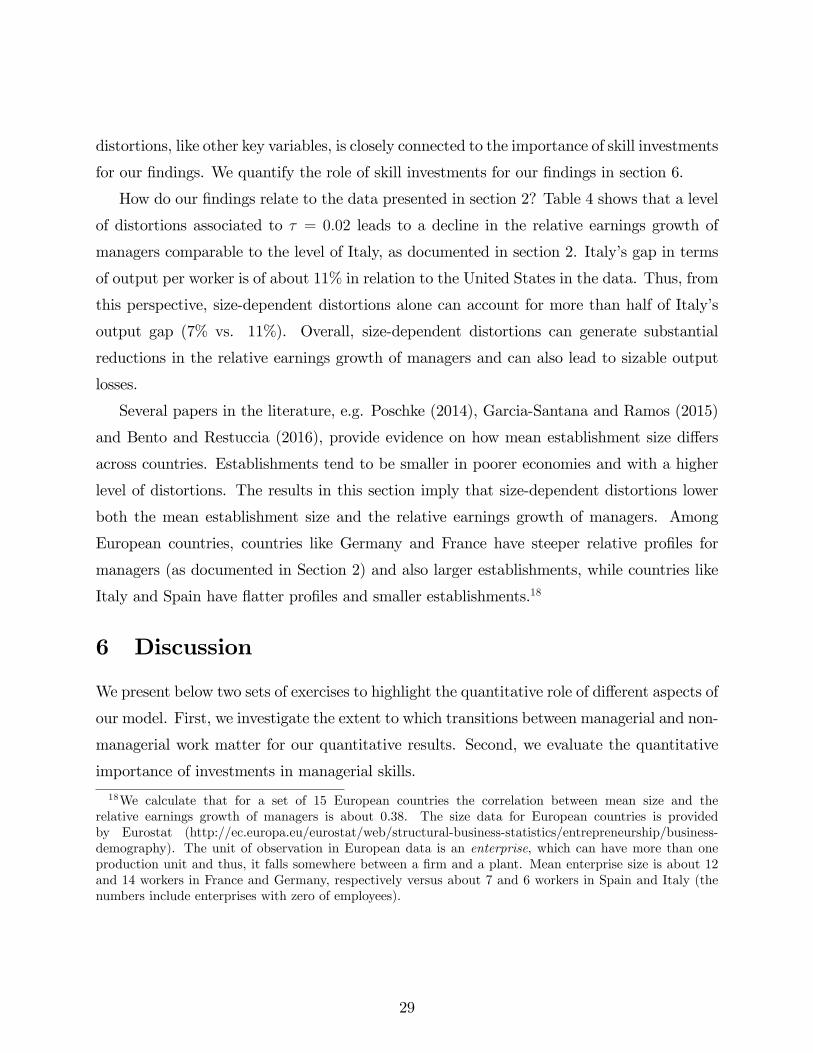
distortions, like other key variables, is closely connected to the importance of skill investments

for our findings. We quantify the role of skill investments for our findings in section 6.

How do our findings relate to the data presented in section 2? Table 4 shows that a level

of distortions associated to τ = 0.02 leads to a decline in the relative earnings growth of

managers comparable to the level of Italy, as documented in section 2. Italy’s gap in terms

of output per worker is of about 11% in relation to the United States in the data. Thus, from

this perspective, size-dependent distortions alone can account for more than half of Italy’s

output gap (7% vs. 11%). Overall, size-dependent distortions can generate substantial

reductions in the relative earnings growth of managers and can also lead to sizable output

losses.

Several papers in the literature, e.g. Poschke (2014), Garcia-Santana and Ramos (2015)

and Bento and Restuccia (2016), provide evidence on how mean establishment size differs

across countries. Establishments tend to be smaller in poorer economies and with a higher

level of distortions. The results in this section imply that size-dependent distortions lower

both the mean establishment size and the relative earnings growth of managers. Among

European countries, countries like Germany and France have steeper relative profiles for

managers (as documented in Section 2) and also larger establishments, while countries like

Italy and Spain have flatter profiles and smaller establishments.18

6 Discussion

We present below two sets of exercises to highlight the quantitative role of different aspects of

our model. First, we investigate the extent to which transitions between managerial and non-

managerial work matter for our quantitative results. Second, we evaluate the quantitative

importance of investments in managerial skills.

18We calculate that for a set of 15 European countries the correlation between mean size and therelative earnings growth of managers is about 0.38. The size data for European countries is providedby Eurostat (http://ec.europa.eu/eurostat/web/structural-business-statistics/entrepreneurship/business-demography). The unit of observation in European data is an enterprise, which can have more than oneproduction unit and thus, it falls somewhere between a firm and a plant. Mean enterprise size is about 12and 14 workers in France and Germany, respectively versus about 7 and 6 workers in Spain and Italy (thenumbers include enterprises with zero of employees).

29

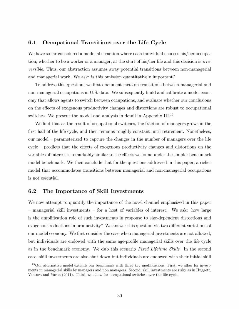
6.1 Occupational Transitions over the Life Cycle

We have so far considered a model abstraction where each individual chooses his/her occupa-

tion, whether to be a worker or a manager, at the start of his/her life and this decision is irre-

versible. Thus, our abstraction assumes away potential transitions between non-managerial

and managerial work. We ask: is this omission quantitatively important?

To address this question, we first document facts on transitions between managerial and

non-managerial occupations in U.S. data. We subsequently build and calibrate a model econ-

omy that allows agents to switch between occupations, and evaluate whether our conclusions

on the effects of exogenous productivity changes and distortions are robust to occupational

switches. We present the model and analysis in detail in Appendix III.19

We find that as the result of occupational switches, the fraction of managers grows in the

first half of the life cycle, and then remains roughly constant until retirement. Nonetheless,

our model —parameterized to capture the changes in the number of managers over the life

cycle —predicts that the effects of exogenous productivity changes and distortions on the

variables of interest is remarkably similar to the effects we found under the simpler benchmark

model benchmark. We then conclude that for the questions addressed in this paper, a richer

model that accommodates transitions between managerial and non-managerial occupations

is not essential.

6.2 The Importance of Skill Investments

We now attempt to quantify the importance of the novel channel emphasized in this paper

—managerial skill investments — for a host of variables of interest. We ask: how large

is the amplification role of such investments in response to size-dependent distortions and

exogenous reductions in productivity? We answer this question via two different variations of

our model economy. We first consider the case when managerial investments are not allowed,

but individuals are endowed with the same age-profile managerial skills over the life cycle

as in the benchmark economy. We dub this scenario Fixed Lifetime Skills. In the second

case, skill investments are also shut down but individuals are endowed with their initial skill

19Our alternative model extends our benchmark with three key modifications. First, we allow for invest-ments in managerial skills by managers and non managers. Second, skill investments are risky as in Huggett,Ventura and Yaron (2011). Third, we allow for occupational switches over the life cycle.

30

endowment at each age. We dub this scenario Fixed Initial Skills.20 We concentrate our

analysis in two special values of distortions and productivity; τ = 0.02 and A = 0.9. These

values are close to the average values in our cross-country analysis in section 7.

Distortions Our findings are summarized in Table 5 for key variables; output, mean

size, managerial quality and the employment share in large (100+) establishments. We find

that managerial skill formation accounts for about one fourth (24-27%) of changes in output

when size-dependent distortions are introduced. This is a significant finding, for investments

in skill formation are less than 1% of output in the benchmark economy.

For size statistics, the message is somewhat different; managerial skill formation accounts

for a smaller fraction of the changes predicted by the benchmark model when distortions

are introduced. For mean size, skill formation accounts for about 9% of the changes under

fixed lifetime skills and nearly 19% under the fixed initial skills scenario. For the share of

employment at large establishments, skill formation accounts for about 24% of the changes

under fixed lifetime skills and nearly 15% under the fixed initial skills scenario. All these

suggest that the economic forces behind a standard span-of-control model tend to dominate

for predicted changes in size statistics.

We find that skill formation has a substantial role upon the predicted changes in man-

agerial quality. Table 5 indicates that about 25%-35% of changes in this variable can be

accounted for by changes in the skills of managers across steady states. In understanding

this finding, recall from our discussion in section 3.3 that changes in this variable is affected

by the number of managers across steady states as well as by changes in the skill distrib-

ution of managers. Thus, while there are large changes in the number of managers due to

size-dependent distortions, the ensuing changes in the incentives to accumulate skills lead to

substantial effects on managerial quality.

Economy-wide Productivity Unlike the findings for distortions, the contribution of

managerial skill formation to changes in output driven by productivity changes is relatively

small (between 6% and 8%). Thus, the bulk of changes in this variable across steady states

in this case are due to standard forces; the direct impact of changes in productivity on output

20For each scenario, we compute a steady state in the absence of distortions and under A = 1. We usethese steady states as the basis for our quantification of the importance of skill investments.

31

plus the indirect effects via capital accumulation.

For the rest of the variables in Table 5, our analysis establishes that managerial skill

formation accounts for all changes across steady states. This is expected. As mentioned

earlier, under a span-of-control model with exogenous managerial skills, exogenous changes

in productivity lead to no changes in the plant-size distribution and therefore, on managerial

quality. Hence, it follows that any change in these variables in response to productivity

changes is driven by the associated changes in managerial skills.

7 Accounting for Cross-Country Differences

We investigated in previous sections the extent to which exogenous variation in productivity

and in size-dependent distortions affect several variables of interest. We now concentrate

on the role of these two exogenous sources of variation for the facts documented in section

2. We ask: what is the contribution of cross-country differences in exogenous productivity

versus distortions in accounting for differences in output per worker and relative earnings

growth? To answer this question, we perform a straightforward exercise. We select values

for productivity (A) and distortions (τ) for each country to reproduce (i) output per worker

levels, and (ii) relative earnings growth (g). That is, we select parameters to reproduce,

as well as we can, the position of each country in Figure 2.21 We then eliminate each of

the cross-country differences separately, and evaluate the quantitative role of each source of

cross-country variation. The average of calibrated values of A is 0.978 across 20 countries in

the sample (recall that for the U.S., A = 1) and the average of calibrated values of τ is 0.028

(recall that for the U.S. τ = 0). The average value for τ implies a wedge, [1− T (5y)] /[1 −T (y)], of 0.96, i.e. a manager that produces five times the mean output faces an average and

marginal distortion (implicit tax) that is four percentage points higher.22

Consider first differences in A, i.e. keep A at its calibrated value for each country and set

21In Figure 2, relative earnings growth for managers is negative for four countries (Finland, Iceland, Spainand Denmark). The model has diffi culty to generate negative relative earnings growth observed in the data.The calibration exercise, nonetheless, is able to match the remaining 16 countries exactly.22The combinations of A and τ that replicate the data differ non trivially across countries. Countries like

Belgium, Italy or Sweden are assigned low A values and positive τ’s to account for the fact that they havelower output per worker and lower income growth of their managers compared to the US. On the other hand,the model assigns low A values and negative τ’s (i.e. distortions decline by size) to be able to match thedata for countries like Germany, France or Switzerland where relative earnings profiles are similar or steeperthan they are in the U.S.

32

τ = 0. Figure 15 shows the model-implied and the actual relation between GDP per worker

and the relative earnings growth of managers. In line with our previous findings, we find that

when we only allow for differences in A, the model predicts a weaker relationship between

output and the relative earnings growth of managers over the life cycle. In particular, while

variation in A is able to generate significant differences in output per worker, the variation in

relative earnings growth is more muted than in the data. As a result, while in the data the

slope coeffi cient between these variables is about 0.57, our model predicts a value of about

0.39 —around the same value as in section 5.1.

Turning into the role of distortions, what happens if we keep τ at its calibrated value

for each country and set A = 1? Figure 16 shows the results of this exercise. The slope

coeffi cient between relative earnings growth and log GDP per worker is now about 0.96,

much higher than the value in the in the data (0.57). That is, in contrast to the case of

variation in A, the model predicts a stronger relationship between log-output per worker and

g than in the data. Indeed, the correlation between data and model-implied relative earnings

growth is about 0.90. In other words, we find that size-dependent distortions are critical to

generate the observed variation in cross-country relative earnings growth of managers.

This exercise allows us to calculate the GDP per worker gap between each country and

the U.S. that can be accounted by differences in A and τ . To this end, we compute GDP

per worker in the model when keeping τ at its calibrated values and setting A = 1 (the

U.S. value), and then calculate the implied output gap with the US and compare it with

the same gap in the data. These calculations, for example, imply that about 43% of the

output gap between Italy and the U.S. can be accounted for by differences in τ . For Sweden,

the equivalent figure is 18%. Repeating the same exercise for other countries, we find that

differences in distortions account on average for about 42% of the output per worker gaps

with the U.S. in our data. The rest is accounted by differences in economy-wide productivity

and interaction effects.

7.1 Discussion: The Role of Initial Managerial Ability

In the previous section, we look for country-specific values of aggregate productivity (A)

and distortions (τ) that can produce the observed cross-country differences in the data.

We do this by following the standard practice in the literature and changing only these

33

two parameters, while keeping all other parameters at their benchmark values. It is of

course understood that there are other possible differences across countries. The analysis, in

particular, assumes that the initial skill distribution is same across countries. Recall that we

assume log(z1) is normally distributed with mean normalized to zero (µz = 0) and variance

σ2z. A natural question is how differences in initial skill distributions would affect our results.

To answer this question, we consider two economies: one in which the mean of the initial

skill distribution is 20% lower and another one in which its coeffi cient of variation is 20%

higher.23 Table 6 shows the results. Consider first an economy with a lower mean for z1.

Since the economy is populated with workers which have lower initial skills, output and the

average managerial quality decline by 7% and 14%, respectively. On the other hand, relative

earnings growth (g) increases, but not by much. Managers who start with relatively low level

of skills invest more aggressively (as a share of GDP), and their earnings grow faster than

they do in the benchmark economy. In equilibrium, in an economy with lower average skills

there are fewer managers and more workers (given all other parameters fixed). Also, the

wage is lower which contributes to a higher growth in managerial incomes and to a larger

firm size. A higher CV of the skill distribution, in contrast, has essentially no effect on

aggregate output. Relative earnings growth and plant size are higher, but again the effects

are quantitatively small. This is not surprising, as a longer right tail of the skill distribution

results in a larger pool of super-star managers who operate larger plants.

Overall, the results in Table 6, while informative about the forces in our model, indicate

that even large differences in the initial skill distributions are not likely to generate significant

differences in output per worker and relative earnings growth of managers across countries.

8 Concluding Remarks

We document that across a group of high-income countries, the mean earnings of managers

tend to grow faster than for non managers over the life cycle, and that the earnings growth

23If log(z1) is normally distributed with µz and σz, the mean and the CV of z1 are given by eµz+

12σ

2z and√

eσ2z − 1, respectively. In the first experiment we simply lower µz (and keep σz the same) so that the mean

is 20% lower, while in the second experiment we increase σz so that the CV is 20% higher (and lower µzso that the mean remains the same). In terms of other distribution of skills across a more diverse set ofcountries, these changes are quite substantial. For instance, the mean math PISA score in the USA is onlyabout 15% higher than in Mexico. Similarly, the coeffi cient of variation is about the same in the US andMexico, and only about 10% in Brazil. See Cubas et al (2016) for an analysis.

34

of managers relative to non managers over the life cycle is positively correlated with output

per worker. To interpret these facts, we develop an equilibrium, span-of-control model in

which managers invest in their skills. Thus, the incentives of managers to invest in their

skills are central in determining the growth of their earnings over the life cycle. As a result,

our model predicts endogenous differences in managerial quality across countries driven by

selection —who becomes a manager —and by investments in managerial skills. We discipline

this model with a host of observations on managerial earnings, the size-distribution of plants

in the United States and macroeconomic aggregates.

We introduce and quantify the importance of aggregate productivity differences, and size-

dependent distortions as emphasized by the misallocation literature. We find that distortions

that halve the growth of relative managerial earnings over the life cycle —the hypothetical

case of Italy in our data —reduce output by 7%. This is more than a half of the observed

output gap between the US and Italy.

Our findings also show that distortions are responsible for the bulk of differences in the

relative earnings growth of managers over the life cycle across countries in our data. As a

result, observations on relative earnings growth can be used as natural targets to discipline

the level of distortions. In a decomposition exercise, we find that cross-country variation

in distortions —estimated to create observed cross-country differences in relative earnings

growth —can account for about 42% of the cross-country variation in output per worker with

the U.S.

References

[1] Akcigit, Ufuk, Alp, Harun and Michael Peters. 2016. “Lack of Selection and Limits to

Delegation: Firm Dynamics in Developing Countries.”NBER Working Paper 21905.

[2] Alder, Simeon D. 2016. "In theWrong Hands: Complementarities, Resources Allocation,

and TFP." American Economic Journal: Macroeconomics, vol. 8(1): 199-241

[3] Atkeson, Andrew and Ariel Burstein, 2015. “Aggregate Implications of Innovation Pol-

icy.”mimeo.

[4] Atkeson, Andrew and Ariel Burstein. 2010. “Innovation, Firm dynamics, and Interna-

tional Trade". Journal of Political Economy, vol. 118(3): 433-484

35

[5] Bartelsman, Eric John Haltiwanger, and Stefano Scarpetta. 2103. “Cross-country Dif-

ferences in Productivity: The Role of Allocation and Selection." American Economic

Review, 103(1): 305—34.

[6] Bauer, Christian and Jose V. Rocriguez Mora. 2014. “The Joint Determination of TFP

and Financial Sector Size.”mimeo.

[7] Benabou, Rolland. 2002. “Tax and Education Policy in a Heterogeneous-Agent Econ-

omy: What Levels of Redistribution Maximize Growth and Effi ciency?”Econometrica

70(2): 481-517.

[8] Bento, Pedro and Diego Restuccia. 2016. “Misallocation, Establishment Size, and Pro-

ductivity." Forthcoming, American Economic Journal: Macroeconomics.

[9] Bhattacharya, Dhritiman, Guner, Nezih and Gustavo Ventura. 2013. "Distortions, En-

dogenous Managerial skills and Productivity Differences." Review of Economic Dynam-

ics, 16(1): 11-25.

[10] Bhattacharya, Dhritiman. 2010. “The Size Distribution of Plants and Economic Devel-

opment.”Unpublished Ph.D. dissertation, The University of Iowa.

[11] Bloom, Nicholas and John Van Reenen. 2011. "Human Resource Management and Pro-

ductivity." In Handbook of Labor Economics, ed. David Card and Orley Ashenfelter,

Amsterdam: Elsevier.

[12] Bloom, Nicholas, Genakos, Christos, Sadun, Raffaella and John Van Reenen. 2012.

"Management Practices across Firms and Countries." Academy of Management Per-

spectives 26(1): 12—33.

[13] Bloom, Nicholas, Sadun, Raffaella and John Van Reenen. 2016. "Management as a

Technology?" NBER Working Paper 22327.

[14] Bloom, Nicholas, Lemos, Renata, Sadun, Raffaella, Scur, Daniela and John Van Reenen.

2014. “The New Empirical Economics of Management.”Journal of the European Eco-

nomic Association, 12(4): 835—876.

36

[15] Buera, Francisco J., Joseph P. Kaboski, and Yongseok Shin. 2011. “Finance and Devel-

opment: A Tale of Two Sectors.”American Economic Review 101(5): 1964-2002.

[16] Caliendo, Lorenzo and Esteban Rossi-Hansberg. 2012. “The Impact of Trade on Orga-

nization and Productivity. ”The Quarterly Journal of Economics 127(3): 1393-1467.

[17] Caselli, Francesco. 2005 “Accounting for Cross-Country Income Differences,”in Hand-

book of Economic Growth, ed. Philippe Aghion and Steven N. Durlauf, Amster-

dam:Elsevier.

[18] Caselli, Francesco, and Nicola Gennaioli. 2013. “Dynastic Management.”Economic In-

quiry, 51(1): 971-996.

[19] Celik, Murat Alp. 2016. “Does the Cream Always Rise to the Top? The Misallocation

of Talent and Innovation.”Mimeo.

[20] Cole, Harold, Jeremy Greenwood and Juan M. Sanchez. 2016. "Why Doesn’t Technology

Flow from Rich to Poor Countries?" Econometrica, 84(4): 1477—1521.

[21] Cubas, Germán, Ravikumar, B. and Gustavo Ventura. 2016. “Talent, Labor Quality

and Economic Development.”Review of Economic Dynamics, 21: 160—181

[22] Deaton, Angus. 1997. The Analysis of Household Surveys: A Microeconometric Ap-

proach to Development Policy. Washington, DC: World Bank Publications.

[23] Erosa, Andrés, Koreshkova, Tatyana and Diego Restuccia. 2010. “How Important is Hu-

man Capital? A Quantitative Theory Assessment of World Income Inequality," Review

of Economic Studies 77(4): 1421-49.

[24] European Union Statistics on Income and Living Conditions (EU-SILC). 2004-2012.

[25] Gabler, Alain and Markus Poschke. 2013. “Experimentation by Firms, Distortions, and

Aggregate Productivity”Review of Economic Dynamics 16(1): 26-38.

[26] Garcia-Santana, Manuel and Roberto Ramos. 2015. "Distortions and the Size Distri-

bution of Plants: Evidence from Cross-Country Data." SERIEs (the Journal of the

Spanish Economic Association) 6(3): 79-312.

37

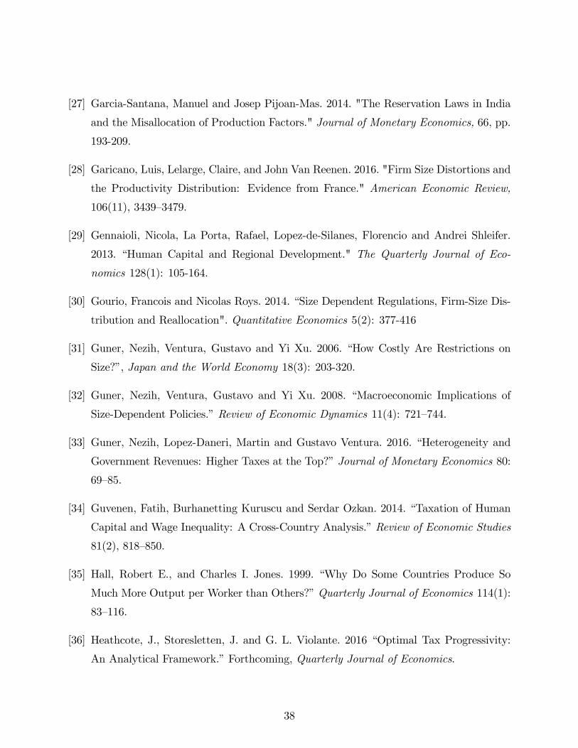
[27] Garcia-Santana, Manuel and Josep Pijoan-Mas. 2014. "The Reservation Laws in India

and the Misallocation of Production Factors." Journal of Monetary Economics, 66, pp.

193-209.

[28] Garicano, Luis, Lelarge, Claire, and John Van Reenen. 2016. "Firm Size Distortions and

the Productivity Distribution: Evidence from France." American Economic Review,

106(11), 3439—3479.

[29] Gennaioli, Nicola, La Porta, Rafael, Lopez-de-Silanes, Florencio and Andrei Shleifer.

2013. “Human Capital and Regional Development." The Quarterly Journal of Eco-

nomics 128(1): 105-164.

[30] Gourio, Francois and Nicolas Roys. 2014. “Size Dependent Regulations, Firm-Size Dis-

tribution and Reallocation". Quantitative Economics 5(2): 377-416

[31] Guner, Nezih, Ventura, Gustavo and Yi Xu. 2006. “How Costly Are Restrictions on

Size?”, Japan and the World Economy 18(3): 203-320.

[32] Guner, Nezih, Ventura, Gustavo and Yi Xu. 2008. “Macroeconomic Implications of

Size-Dependent Policies.”Review of Economic Dynamics 11(4): 721—744.

[33] Guner, Nezih, Lopez-Daneri, Martin and Gustavo Ventura. 2016. “Heterogeneity and

Government Revenues: Higher Taxes at the Top?”Journal of Monetary Economics 80:

69—85.

[34] Guvenen, Fatih, Burhanetting Kuruscu and Serdar Ozkan. 2014. “Taxation of Human

Capital and Wage Inequality: A Cross-Country Analysis.”Review of Economic Studies

81(2), 818—850.

[35] Hall, Robert E., and Charles I. Jones. 1999. “Why Do Some Countries Produce So

Much More Output per Worker than Others?”Quarterly Journal of Economics 114(1):

83—116.

[36] Heathcote, J., Storesletten, J. and G. L. Violante. 2016 “Optimal Tax Progressivity:

An Analytical Framework.”Forthcoming, Quarterly Journal of Economics.

38

[37] Hopenhayn, Hugo. A. 2014. "Firms, Misallocation and Aggregate Productivity: A Re-

view." Annual Review of Economics 6: 735-770.

[38] Hsieh, Chang-Tai, and Peter Klenow. 2009. “Misallocation and Manufacturing TFP in

China and India.”Quarterly Journal of Economics 124(4): 1403—1448.

[39] Hsieh, Chang-Tai and Peter Klenow. 2014. “The Life Cycle of Plants in India and

Mexico.”Quarterly Journal of Economics 129(3): 1035—1084.

[40] Huggett, Mark, Gustavo Ventura, and Amir Yaron. 2011. “Sources of Lifetime Inequal-

ity.”American Economic Review 101(7): 2923—2954.

[41] Jones, Charles I. and Jihee Kim. 2017. “A Schumpeterian Model of Top Income In-

equality.”mimeo.

[42] Klenow, Peter J., and Andres Rodrıguez-Clare. 1997. “The Neoclassical Revival in

Growth Economics: Has it Gone Too Far?” In Macroeconomics Annual 1997. , ed.

Ben S. Bernanke and Julio J. Rotemberg, 73—102. Cambridge:MIT Press.

[43] Lagakos, David, Moll, Benjamin, Porzio, Tommaso, Qian, Nancy and Todd Schoellman.

2016. “Life-Cycle Wage Growth Across Countries.”Forthcoming, Journal of Political

Economy.

[44] Lucas, Jr., Robert E. 1978. “On the Size Distribution of Business Firms.”Bell Journal

of Economics, 9(2): 508—523.

[45] Luxembourg Income Study (LIS) Database, http://www.lisdatacenter.org (multiple

countries; microdata accessed from November 2013 to February 2017). Luxembourg:

LIS.

[46] Manuelli, Rodolfo and Ananth Seshadri. 2014. “Human Capital and the Wealth of

Nations." American Economic Review 104(9): 2736-62.

[47] Midrigan, Virgiliu and Yi Xu . 2010. “Finance and Misallocation: Evidence from Plant-

level Data.”American Economic Review, 104(2): 422-58.

[48] Minnesota Population Center. 2014. Integrated Public Use Microdata Series, Interna-

tional: Version 6.3 [Machine-readable database]. Minneapolis: University of Minnesota.

39

[49] Prescott, Edward. 1998. “Needed: A Theory of Total Factor Productivity.”International

Economic Review, 39(3): 525—551.

[50] Restuccia, Diego. 2013. "Factor Misallocation and Development," The New Palgrave

Dictionary of Economics, Online Edition, Eds. Steven N. Durlauf and Lawrence E.

Blume, Palgrave Macmillan.

[51] Restuccia, Diego, and Richard Rogerson. 2008. “Policy Distortions and Aggregate Pro-

ductivity with Heterogeneous Establishments.”Review of Economic Dynamics, 11(4):

707—720.

[52] Restuccia, Diego, and Richard Rogerson. 2013. "Misalloaction and Productivity." Re-

view of Economic Dynamics, 16(1): 1-10.

[53] Roys, Nicolas and Ananth Seshadri. 2014. " Economic Development and the Organiza-

tion of Production." mimeo.

[54] Rubini, Loris. 2014. ““Innovation and the Trade Elasticity." Journal of Monetary Eco-

nomics, 66, pp. 32-46.

[55] Ruggles, Steven, J. Trent Alexander, Katie Genadek, Ronald Goeken, Matthew B.

Schroeder, and Matthew Sobek. 2010. Integrated Public Use Microdata Series: Version

5.0 [Machine-readable database]. Minneapolis: University of Minnesota.

[56] Shimer, Robert. 2012. "Reassessing the Ins and Outs of Unemployment." Review of

Economic Dynamics 15: 127-148.

40

Table 1: Parameter Values (annualized)

Parameter ValuesPopulation Growth Rate (gN) 0.011Productivity Growth Rate (g) 0.026Depreciation Rate (δ) 0.040Skill accumulation technology (δz) 0.048Importance of Capital (α) 0.423Returns to Scale (γ) 0.77Mean Log-managerial Ability (µz) 0Dispersion in Log-managerial Ability (σz) 2.800Discount Factor (β) 0.944Skill accumulation technology (θ) 0.881Skill accumulation technology (δθ) 0.053Skill accumulation technology (θ1) 0.68Skill accumulation technology (θ2) 0.49

Note: Entries show model parameters calibrated for the benchmark economy. See text for

details.

Table 2: Empirical Targets: Model and Data

Statistic Data ModelMean Size 17.9 17.7Capital Output Ratio 2.32 2.32Relative Earnings Growth (g) (40-44/25-29) 0.168 0.168Relative Earnings Growth (g) (60-64/25-29) 0.221 0.212Capital Share 0.326 0.326Fraction of Establishments1-9 workers 0.725 0.72610-20 workers 0.126 0.12820-50 workers 0.091 0.08550-100 workers 0.032 0.031100+ workers 0.026 0.030Employment Share1-9 workers 0.151 0.17210-20 workers 0.094 0.10020-50 workers 0.164 0.14850-100 workers 0.128 0.121100+ workers 0.462 0.459

Note: Entries show the empirical targets used in the quantitative analysis and the model’s

performance. The fraction of establishments with 1-9 and 100+ workers, and the employment

share with 100+ workers are explicit targets. See text for details.

41

Table 3: Effects of Economy-Wide Productivity

Economy-Wide Productivity A= 1 A= 0.9 A= 0.8 A= 0.7

StatisticOutput 100 84.5 70.2 56.9Mean Size 17.7 17.2 17.0 16.0Investment in Skills 100 73.3 52.1 35.3Investment in Skills (% Output) 0.92 0.80 0.68 0.57Number of Managers 100 102.9 102.9 105.8Managerial Quality 100 93.6 90.1 84.6Employment Share (100+) 0.46 0.45 0.44 0.43Relative Earnings Growth (g) 0.22 0.16 0.10 0.04

Note: Entries show the effects on displayed variables associated to exogenous reductions in the

level of economy-wide productivity (A) across steady states. Column 2 report benchmark values

(A = 1). Column 3-5 report the changes emerging from reducing A below the benchmark value.

See text for details.

Table 4: Effects of Size-Dependent Distortions

Size Dependency (τ) 0 0.02 0.04 0.06 0.08

Tax Wedge(1−T (5y)1−T (y)

)1 0.97 0.94 0.91 0.88

StatisticOutput 100.0 92.9 86.7 81.3 76.2Mean Size 17.7 13.2 10.2 8.2 6.8Investment in Skills 100.0 62.1 41.6 29.6 22.1Investment in Skills (% Output) 0.92 0.61 0.44 0.33 0.27Number of Managers 100.0 131.9 166.9 203.4 239.8Managerial Quality 100.0 73.2 56.6 45.6 38.2Employment Share (100+) 0.46 0.34 0.25 0.17 0.11Relative Earnings Growth (g) 0.22 0.09 0.02 -0.02 -0.05

Note: Entries show the effects on displayed variables associated to size-dependent distortions

across steady states. Column 2 report benchmark values. Column 3-6 report the changes emerging

from increasing the size dependency of distortions. See text for details.

42

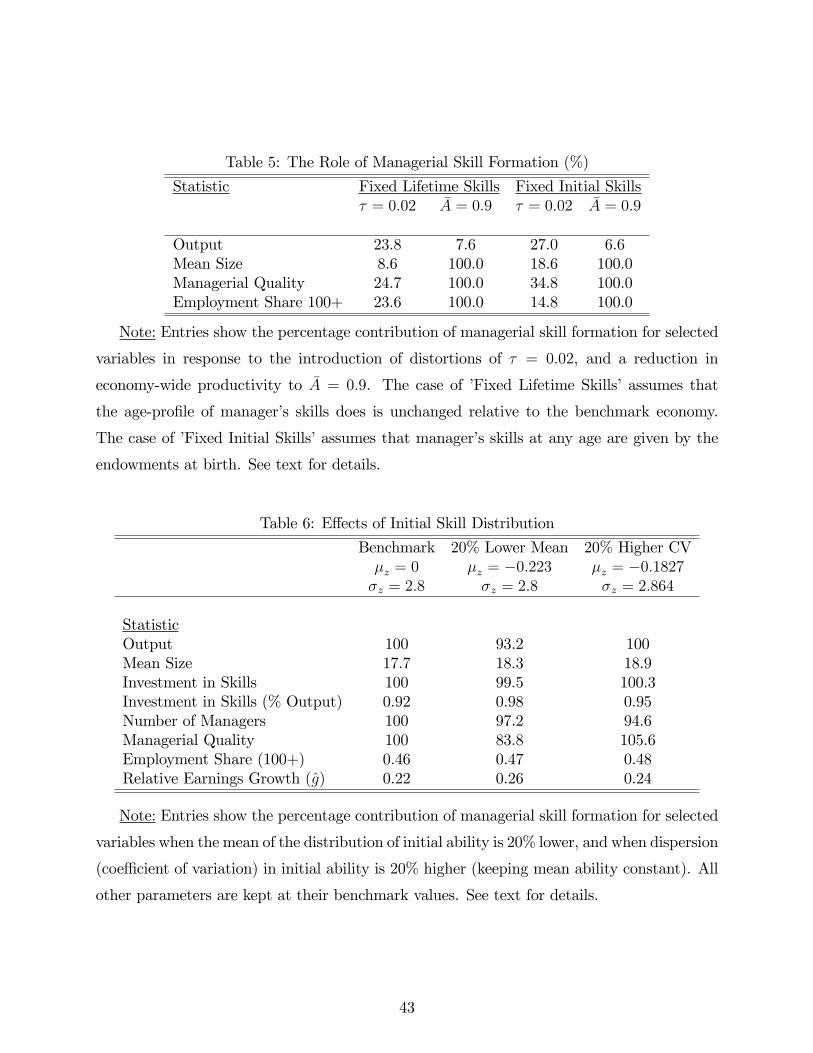
Table 5: The Role of Managerial Skill Formation (%)

Statistic Fixed Lifetime Skills Fixed Initial Skillsτ = 0.02 A = 0.9 τ = 0.02 A = 0.9

Output 23.8 7.6 27.0 6.6Mean Size 8.6 100.0 18.6 100.0Managerial Quality 24.7 100.0 34.8 100.0Employment Share 100+ 23.6 100.0 14.8 100.0

Note: Entries show the percentage contribution of managerial skill formation for selected

variables in response to the introduction of distortions of τ = 0.02, and a reduction in

economy-wide productivity to A = 0.9. The case of ’Fixed Lifetime Skills’assumes that

the age-profile of manager’s skills does is unchanged relative to the benchmark economy.

The case of ’Fixed Initial Skills’assumes that manager’s skills at any age are given by the

endowments at birth. See text for details.

Table 6: Effects of Initial Skill Distribution

Benchmark 20% Lower Mean 20% Higher CVµz = 0 µz = −0.223 µz = −0.1827σz = 2.8 σz = 2.8 σz = 2.864

StatisticOutput 100 93.2 100Mean Size 17.7 18.3 18.9Investment in Skills 100 99.5 100.3Investment in Skills (% Output) 0.92 0.98 0.95Number of Managers 100 97.2 94.6Managerial Quality 100 83.8 105.6Employment Share (100+) 0.46 0.47 0.48Relative Earnings Growth (g) 0.22 0.26 0.24

Note: Entries show the percentage contribution of managerial skill formation for selected

variables when the mean of the distribution of initial ability is 20% lower, and when dispersion

(coeffi cient of variation) in initial ability is 20% higher (keeping mean ability constant). All

other parameters are kept at their benchmark values. See text for details.

43

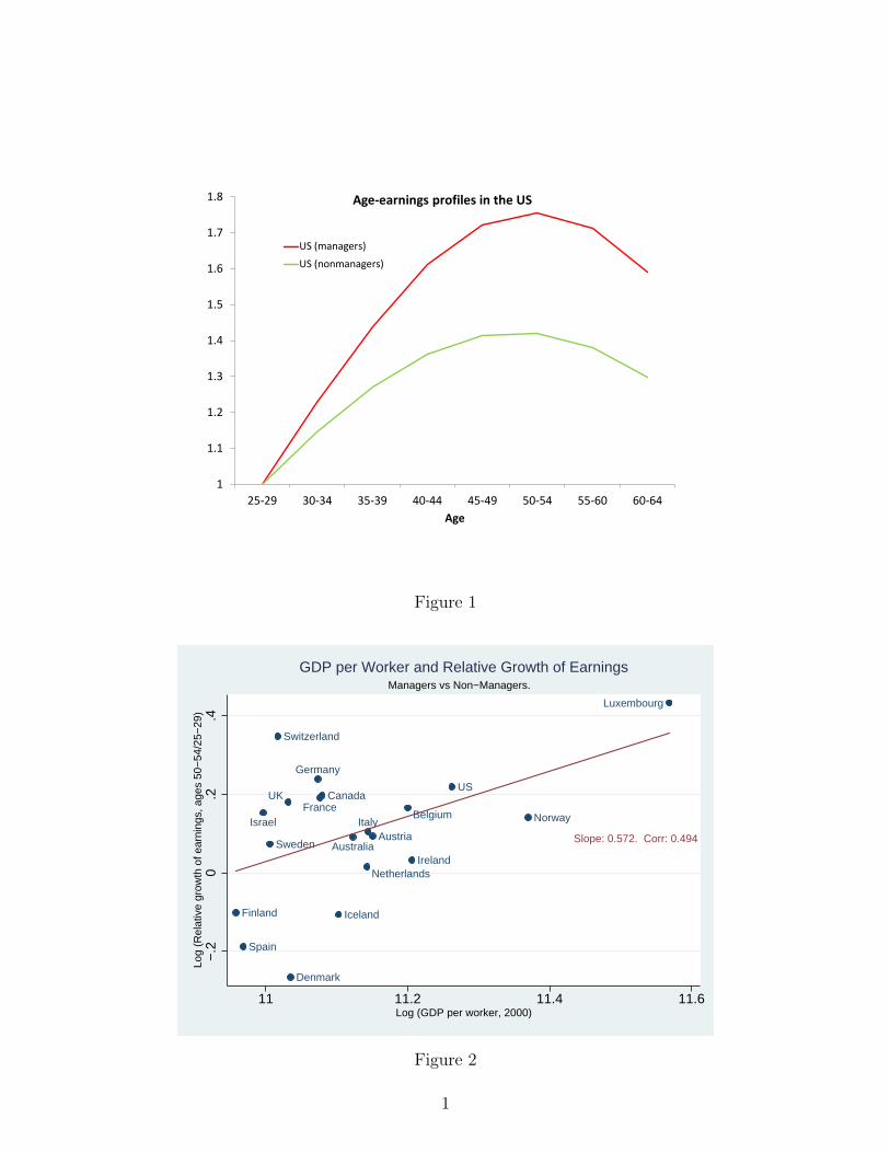
1

1.1

1.2

1.3

1.4

1.5

1.6

1.7

1.8

25-29 30-34 35-39 40-44 45-49 50-54 55-60 60-64

Age

Age-earnings profiles in the US

US (managers)

US (nonmanagers)

Figure 1

AustraliaAustria

Belgium

Canada

Denmark

Finland

France

Germany

Iceland

Ireland

Israel Italy

Luxembourg

Netherlands

Norway

Spain

Sweden

Switzerland

UKUS

−.2

0.2

.4Lo

g (R

elat

ive

grow

th o

f ear

ning

s, a

ges

50−

54/2

5−29

)

11 11.2 11.4 11.6Log (GDP per worker, 2000)

Slope: 0.572. Corr: 0.494

Managers vs Non−Managers.

GDP per Worker and Relative Growth of Earnings

Figure 2

1

Australia

CanadaFrance

Germany

Ireland

Italy

Spain

Sweden

UK

US

−.2

−.1

0.1

.2.3

Log

(Rel

ativ

e gr

owth

of m

anag

ers’

ear

ning

s, a

ges

50−

54/2

5−29

)

2.8 3 3.2 3.4Management Practices Score: Bloom et al (2012 and 2014)

Slope: 0.572. Corr: 0.793

Management Practices and Relative Income Growth

Figure 3

AustraliaAustria

Belgium

Canada

Denmark

Finland

France

Germany

Iceland

Ireland

Israel Italy

Luxembourg

Netherlands

Norway

Spain

Sweden

Switzerland

UKUS

−.2

0.2

.4Lo

g (R

elat

ive

grow

th o

f ear

ning

s, a

ges

50−

54/2

5−29

)

11 11.2 11.4 11.6Log (GDP per worker, 2000)

Slope: 0.506. Corr: 0.483

Managers vs Non−Managers. Weighted by size of workforce

GDP per Worker and Relative Growth of Earnings

Figure 4

2

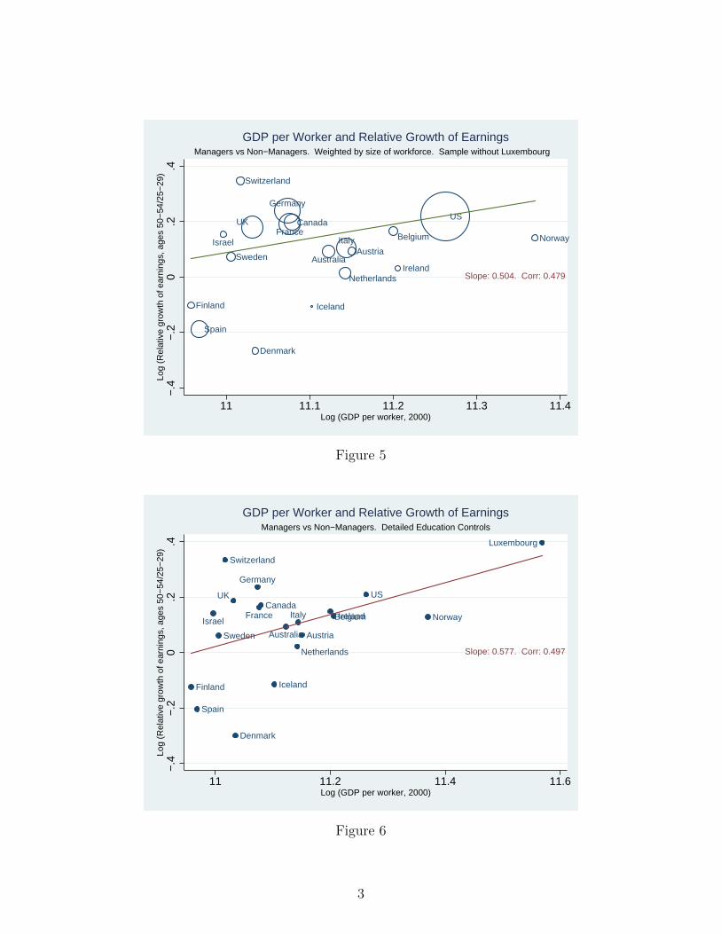
AustraliaAustria

Belgium

Canada

Denmark

Finland

France

Germany

Iceland

Ireland

Israel Italy

Netherlands

Norway

Spain

Sweden

Switzerland

UKUS

−.4

−.2

0.2

.4Lo

g (R

elat

ive

grow

th o

f ear

ning

s, a

ges

50−

54/2

5−29

)

11 11.1 11.2 11.3 11.4Log (GDP per worker, 2000)

Slope: 0.504. Corr: 0.479

Managers vs Non−Managers. Weighted by size of workforce. Sample without Luxembourg

GDP per Worker and Relative Growth of Earnings

Figure 5

Australia Austria

BelgiumCanada

Denmark

Finland

France

Germany

Iceland

IrelandIsraelItaly

Luxembourg

Netherlands

Norway

Spain

Sweden

Switzerland

UK US

−.4

−.2

0.2

.4Lo

g (R

elat

ive

grow

th o

f ear

ning

s, a

ges

50−

54/2

5−29

)

11 11.2 11.4 11.6Log (GDP per worker, 2000)

Slope: 0.577. Corr: 0.497

Managers vs Non−Managers. Detailed Education Controls

GDP per Worker and Relative Growth of Earnings

Figure 6

3

Australia Austria

BelgiumCanada

Denmark

Finland

France

Germany

Iceland

Ireland

Israel Italy

Luxembourg

Netherlands

Norway

Spain

Sweden

Switzerland

UK US

−.4

−.2

0.2

.4Lo

g (R

elat

ive

grow

th o

f ear

ning

s, a

ges

50−

54/2

5−29

)

11 11.2 11.4 11.6Log (GDP per worker, 2000)

Slope: 0.591. Corr: 0.509

Managers vs Non−Managers. Industry and Detailed Education Controls

GDP per Worker and Relative Growth of Earnings

Figure 7

AustraliaAustria

Belgium

Canada

Denmark

Finland

FranceGermany

Iceland

Ireland

Israel

Italy

Luxembourg

Netherlands

NorwaySpain

Sweden

Switzerland

UKUS

−.2

0.2

.4.6

Log

(Rel

ativ

e gr

owth

of e

arni

ngs,

age

s 50

−54

/25−

29)

11 11.2 11.4 11.6Log (GDP per worker, 2000)

Slope: 0.691. Corr: 0.497

Managers vs Non−Managers, Excluding Self−Employed.

GDP per Worker and Relative Growth of Earnings

Figure 8

4

AustraliaAustriaBelgium

Canada

Denmark

Finland

France

Germany

Iceland

Ireland

Israel

Italy

Luxembourg

Netherlands

Norway

Spain

Sweden

Switzerland

UKUS

−.4

−.2

0.2

.4Lo

g (R

elat

ive

grow

th o

f ear

ning

s, a

ges

50−

54/2

5−29

)

11 11.2 11.4 11.6Log (GDP per worker, 2000)

Slope: 0.587. Corr: 0.458

Managers vs Non−Managers, Excluding Self−Employed Non−Managers.

GDP per Worker and Relative Growth of Earnings

Figure 9

Australia

Austria

Belgium

Canada

Denmark

Finland

FranceGermany

Iceland

Ireland

Israel

ItalyLuxembourg

Netherlands

NorwaySpain

Sweden

Switzerland

UK US

−.4

−.2

0.2

.4.6

Log

(Rel

ativ

e gr

owth

of e

arni

ngs,

age

s 50

−54

/25−

29)

11 11.2 11.4 11.6Log (GDP per worker, 2000)

Slope: 0.633. Corr: 0.500

Managers vs Non−Managers, Wage and Salary Income Only.

GDP per Worker and Relative Growth of Earnings

Figure 10

5

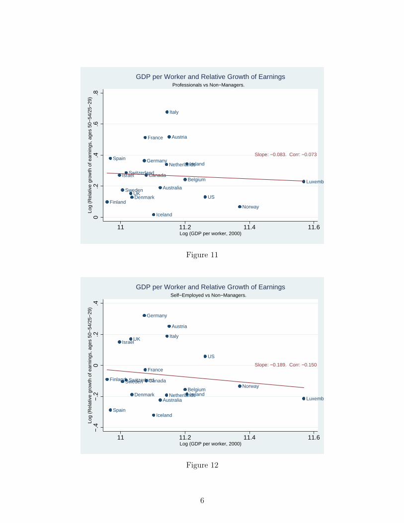
Australia

Austria

BelgiumCanada

DenmarkFinland

France

Germany

Iceland

Ireland

Israel

Italy

Luxembourg

Netherlands

Norway

Spain

Sweden

Switzerland

UKUS

0.2

.4.6

.8Lo

g (R

elat

ive

grow

th o

f ear

ning

s, a

ges

50−

54/2

5−29

)

11 11.2 11.4 11.6Log (GDP per worker, 2000)

Slope: −0.083. Corr: −0.073

Professionals vs Non−Managers.

GDP per Worker and Relative Growth of Earnings

Figure 11

Australia

Austria

Belgium

Canada

Denmark

Finland

France

Germany

Iceland

Ireland

IsraelItaly

LuxembourgNetherlands

Norway

Spain

SwedenSwitzerland

UK

US

−.4

−.2

0.2

.4Lo

g (R

elat

ive

grow

th o

f ear

ning

s, a

ges

50−

54/2

5−29

)

11 11.2 11.4 11.6Log (GDP per worker, 2000)

Slope: −0.189. Corr: −0.150

Self−Employed vs Non−Managers.

GDP per Worker and Relative Growth of Earnings

Figure 12

6

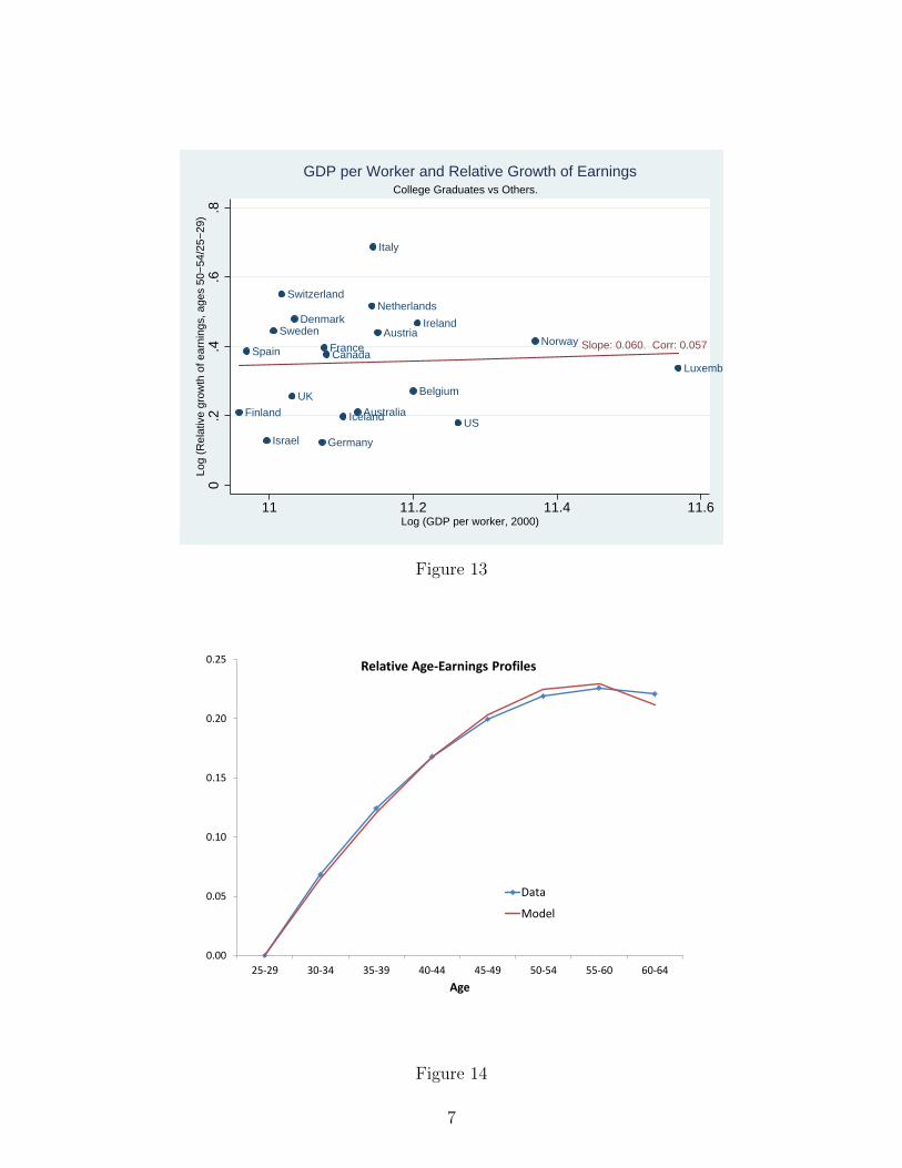
Australia

Austria

Belgium

Canada

Denmark

Finland

France

Germany

Iceland

Ireland

Israel

Italy

Luxembourg

Netherlands

NorwaySpain

Sweden

Switzerland

UK

US

0.2

.4.6

.8Lo

g (R

elat

ive

grow

th o

f ear

ning

s, a

ges

50−

54/2

5−29

)

11 11.2 11.4 11.6Log (GDP per worker, 2000)

Slope: 0.060. Corr: 0.057

College Graduates vs Others.

GDP per Worker and Relative Growth of Earnings

Figure 13

0.00

0.05

0.10

0.15

0.20

0.25

25-29 30-34 35-39 40-44 45-49 50-54 55-60 60-64

Age

Relative Age-Earnings Profiles

Data

Model

Figure 14

7

−.2

0.2

.4Lo

g (I

ncom

e G

row

th, 5

0−54

/25−

29)

−.4 −.2 0 .2 .4Log (GDP per Worker, 2000)

data model

A calibrated, tau=0Data vs Model

Figure 15

−.2

0.2

.4.6

Log

(Inc

ome

Gro

wth

, 50−

54/2

5−29

)

−.4 −.2 0 .2 .4Log (GDP per Worker, 2000)

data model

A=1, tau calibratedData vs Model

Figure 16

8

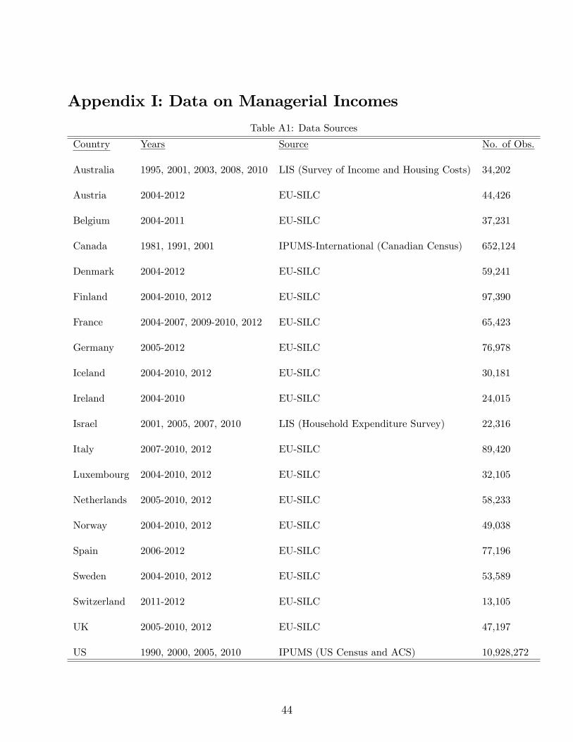
Appendix I: Data on Managerial Incomes

Table A1: Data Sources

Country Years Source No. of Obs.

Australia 1995, 2001, 2003, 2008, 2010 LIS (Survey of Income and Housing Costs) 34,202

Austria 2004-2012 EU-SILC 44,426

Belgium 2004-2011 EU-SILC 37,231

Canada 1981, 1991, 2001 IPUMS-International (Canadian Census) 652,124

Denmark 2004-2012 EU-SILC 59,241

Finland 2004-2010, 2012 EU-SILC 97,390

France 2004-2007, 2009-2010, 2012 EU-SILC 65,423

Germany 2005-2012 EU-SILC 76,978

Iceland 2004-2010, 2012 EU-SILC 30,181

Ireland 2004-2010 EU-SILC 24,015

Israel 2001, 2005, 2007, 2010 LIS (Household Expenditure Survey) 22,316

Italy 2007-2010, 2012 EU-SILC 89,420

Luxembourg 2004-2010, 2012 EU-SILC 32,105

Netherlands 2005-2010, 2012 EU-SILC 58,233

Norway 2004-2010, 2012 EU-SILC 49,038

Spain 2006-2012 EU-SILC 77,196

Sweden 2004-2010, 2012 EU-SILC 53,589

Switzerland 2011-2012 EU-SILC 13,105

UK 2005-2010, 2012 EU-SILC 47,197

US 1990, 2000, 2005, 2010 IPUMS (US Census and ACS) 10,928,272

44

Table A2: Managerial Occupations

AustraliaBefore 2001, International Standard Classification of Occupations (ISCO-88), Codes 11-13Legislators, senior offi cials and managersCorporate managersManagers of small enterprisesAfter 2001, ASCO, occupation code 1Managers and administrators

Austria, Belgium, Canada, Denmark, Finland, France, Germany, Iceland, IrelandIsrael, Italy, Luxembourg, Netherlands, Norway, Spain, Sweden, Switzerland, UKInternational Standard Classification of Occupations (ISCO-88), Codes 11-13Legislators, senior offi cials and managersCorporate managersManagers of small enterprises

USIPUMS-USA 1990 Occupation Codes 004-022Chief executives and public administrators, Financial managers,Human resources and labor relations managers, Managers and Specialists in marketing,advertising, and public relations, Managers in education and related fields, Managers ofmedicine and health occupations, Postmasters and mail superintendents, Managers of foodservices and lodging occupations, Managers of properties and real estate, Funeral directors,Managers of service organizations, Managers and administrators

45

Appendix II: Balanced Growth

Along a balanced growth path (i) growth rates are constant; (ii) the growth rate in output

equals the growth rate in labor and managerial income; (iii) growth in aggregate skill in-

vestment is the same as the growth rate in output; (iv) the capital-output ratio is constant;

(v) the fractions of managers and workers are constant (i.e. z∗(t) = z∗ for all t); (vi) factor

prices are constant.

We find the growth rate in output per person (g) and initial managerial skills (gz) consis-

tent with (i)-(vi), given a growth rate in exogenous productivity (gA). Specifically, we show

that there is a balanced growth path if and only if initial managerial skills grow at a specific

rate determined by exogenous productivity growth.

From the properties of the plant’s technology, it follows that

1 + g = (1 + gA) (1 + gz)1−γ(1 + gk)

αγ,

where gk stands for the growth rate of capital per person. It follows that

1 + g = (1 + gA)1

1−αγ (1 + gz)1−γ1−αγ (24)

We proceed now to find the rate of growth of managerial skills that is consistent with

a balanced-growth path. We denote by g∗z such growth rate. Note that if such path exists,

then the age profile is shifted by a time-invariant factor (1 + g∗z). That is,

zj(t+ 1)

zj(t)= (1 + g∗z)

for all j = 1, ...JR − 1. It follows that we can infer the value of g∗z from the first-order

conditions for skill investments of two cohorts of age j ≤ JR − 2, at two consecutive dates.

In particular, the first-order condition for decisions at the penultimate period of the working

life cycle must hold along a balanced-growth path. From (13), it follows:(1

1 + g∗z

)θ1( 1

1 + g

)θ2−1= (1 + g∗A)

11−γ

(1

1 + g

) γ(1−α)1−γ

. (25)

46

In deriving the expression above, we used the fact that along a balanced growth path, the

rate of return is constant and that the growth in output per capita, g, equals the growth rate

in skill investments and the growth rate in wage rates. Solving for g∗z in (25), we obtain:

1 + g∗z = (1 + g)γ(1−α)+(1−θ2)(1−γ)

θ1(1−γ)

(1

1 + gA

) 1θ1(1−γ)

(26)

Substituting (26) in (24), after algebra we obtain

1 + g = (1 + gA)ψ,

where ψ

ψ ≡ 1− θ1γ(1− α) + (1− θ2)(1− γ)− θ1(1− αγ)

. (27)

Comments Several points are worth noting from the expression above. First, there is

balanced growth path with positive growth in per capita output as long as θ1 ∈ [0, 1). Second,

all the same, the growth rate in output per capita increases with θ2: as the importance of

investments in the production of new skills increases, the growth rate in output per capita

increases as well. Indeed, as θ2 → 0,

ψ → 1

1− αγ .

That is, the growth rate approaches the growth rate with exogenous skill investments

given by the reciprocal of one minus the capital share.

Finally, as the span-of-control parameter approaches 1,

ψ → 1

1− α,

which results in the growth rate of a standard economy with constant returns in capital andlabor.

47

Appendix III: Occupational Transitions

In the benchmark economy presented in detail in Section 3, each individual chooses his/her

occupation, whether to be a worker or a manager, at the start of his/her life and this decision

is irreversible. In this Appendix, we first document facts on transitions between managerial

and non-managerial occupations for the U.S., and then build and calibrate a model economy

that allows agents to switch between occupations. Finally, we study, as we did in sections

5.1 and 5.2, the effects of changes in economy-wide productivity (A) and the size dependence

of distortions.

8.1 Data on Occupational Transitions

In order to compute transitions between managerial and non-managerial occupations in the

United States, we use data from the Outgoing Rotation Groups of the Current Popula-

tion Survey (CPS) for 1990-2010 period. Every household (address) that enters the CPS is

interviewed for 4 consecutive months, then ignored (rotated out) for 8 months, and then in-

terviewed again (rotated in) for 4 more months. As a result, it is possible to have observation

on a subset of CPS sample that is one year apart. We follow a standard matching procedure,

specified in Shimer (2012), based on matching households with the same identification code,

as long as household members’characteristics (age, sex, race and education) are consistent

between two points in time. The sample consists of individuals aged 25-64 who work at least

30 hours a week.

Based on matched households, we compute the fraction of individuals between ages 25-

29, 30-34,..., 60-64 who transit from a managerial (non-managerial occupations) to a non-

managerial (managerial) occupation within a year. A transition from managerial (non-

managerial) to non-managerial (managerial) occupation occurs if in month t a worker reports

an occupation that belongs to the set of managerial (non-managerial) occupations, while

in month t + 12 he/she reports an occupation that belongs to the set of non-managerial

(managerial) occupations. The classification that we use to distinguish between managerial

and non-managerial occupations is detailed in Section 2. If a worker is not observed or does

not report any occupation in the year, he is excluded from the sample we use to calculate

the transitions. We report average yearly transitions for 1990-2010 period.

Figure 1 shows the transitions between occupations in our data. As the figure shows, there

48

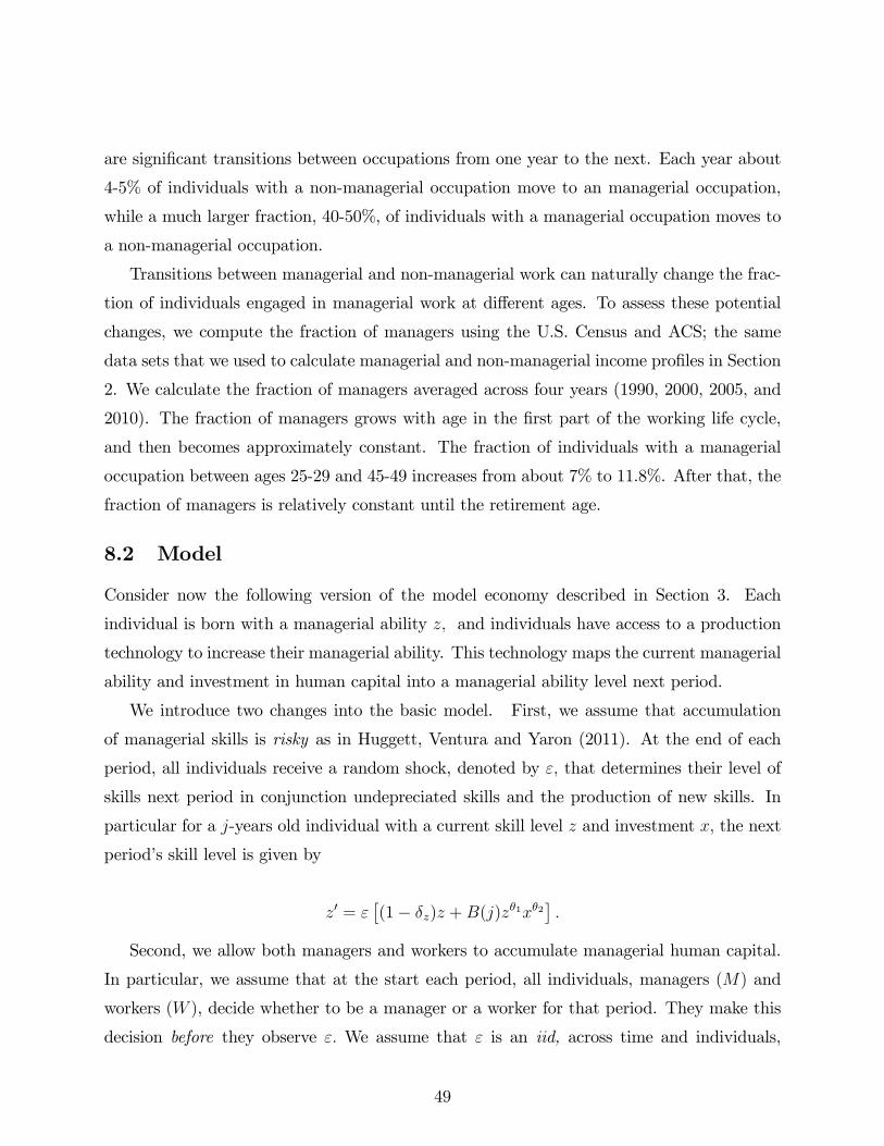
are significant transitions between occupations from one year to the next. Each year about

4-5% of individuals with a non-managerial occupation move to an managerial occupation,

while a much larger fraction, 40-50%, of individuals with a managerial occupation moves to

a non-managerial occupation.

Transitions between managerial and non-managerial work can naturally change the frac-

tion of individuals engaged in managerial work at different ages. To assess these potential

changes, we compute the fraction of managers using the U.S. Census and ACS; the same

data sets that we used to calculate managerial and non-managerial income profiles in Section

2. We calculate the fraction of managers averaged across four years (1990, 2000, 2005, and

2010). The fraction of managers grows with age in the first part of the working life cycle,

and then becomes approximately constant. The fraction of individuals with a managerial

occupation between ages 25-29 and 45-49 increases from about 7% to 11.8%. After that, the

fraction of managers is relatively constant until the retirement age.

8.2 Model

Consider now the following version of the model economy described in Section 3. Each

individual is born with a managerial ability z, and individuals have access to a production

technology to increase their managerial ability. This technology maps the current managerial

ability and investment in human capital into a managerial ability level next period.

We introduce two changes into the basic model. First, we assume that accumulation

of managerial skills is risky as in Huggett, Ventura and Yaron (2011). At the end of each

period, all individuals receive a random shock, denoted by ε, that determines their level of

skills next period in conjunction undepreciated skills and the production of new skills. In

particular for a j-years old individual with a current skill level z and investment x, the next

period’s skill level is given by

z′ = ε[(1− δz)z +B(j)zθ1xθ2

].

Second, we allow both managers and workers to accumulate managerial human capital.

In particular, we assume that at the start each period, all individuals, managers (M) and

workers (W ), decide whether to be a manager or a worker for that period. They make this

decision before they observe ε. We assume that ε is an iid, across time and individuals,

49

shock distributed according to a cumulative distribution function Go(ε), o ∈ W,M. Oncethe individuals make their occupation choice, they decide how much to consume, how much

to save and how much to invest to enhance their skills, x. They make all these decisions

again before they observe ε. After the investment decisions are made, ε is realized and the

individuals enter next period with their updated level of human capital. Then they again

make an occupational choice decision and so on.

In this environment, although managerial skills do not affect the current income of work-

ers, as they simply earn w, they still have an incentive to invest in their skills as a favorable

ε shock in the future can make them switch occupations next period. A manager, on the

other hand, can decide to become a worker if his/her ε was too low last period. We assume

that switching occupation has no monetary or utility cost.

Consider the problem of an age-j individual. At the start of the of the period, given his

current skills (z) and assets (a), this individual decides whether to be a manager to a worker:

V (a, z, j) = maxV M(a, z, j), V W (a, z, j)

.

The value of being a manager V M(a, z, j) is given by

V M(a, z, j) = maxc,a′,x

u(c) + β

∫V (a′, z′(ε), j + 1)dGM(ε)

,

subject to

c+ a′ + x ≤ π(z, r, w) + (1 + r)a,

and

z′ = ε[(1− δz)z +B(j)zθ1xθ2

],

where π(z, r, w) is the profits of managers as defined by equation 6 in Section 3.1.

The value of being a worker V W (a, z, j), on the other hand, is given by

V W (a, z, j) = maxc,a′,x

u(c) + β

∫V (a′, z′(ε), j + 1)dGW (ε)

,

subject to

c+ a′ + x ≤ w + (1 + r)a,

and

z′ = ε[(1− δz)z +B(j)zθ1xθ2

]50

8.3 Parameter Values

We follow the same calibration strategy as described in Section 4. In addition to the pa-

rameters listed in Table 1, we need to specify the functional forms for GM(ε) and GW (ε).

We assume that both distributions are log-normal with mean zero and variances denoted

by ξM and ξW . In the model economy, these variances have implications for the fraction

of managers in the labor force at each age as well as the relative age-earnings profile of

managers. As a result, in order to calibrate these parameters we select two new targets: i)

the fraction of managers at age 60-64 relative to the fraction of managers at age 25-29 and

ii) an additional moment from the age-earnings profile —the relative earnings at age 50-54

(recall that relative incomes at ages 40-44 and 60-64 were already among the targets in Table

2). Table A3 presents the calibrated parameters of the model with occupational transitions.

Table A4 compares the data and the model moments. The model captures endogenously

the growth in the number of managers by age. Both the model and the data, the fraction of

population with fraction of individuals with a managerial occupation increases by a factor

of 1.63 between ages 25-29 to 60-64. Figure 2 shows the relative age-earnings profiles of

managers in the model and the data. The model matches very well the age-earnings profiles

of managers.

With a few exceptions parameter values in Tables 1 and A3 are quite similar. In partic-

ular, the span of control parameter γ is larger in the economy with occupational transitions.

The volatility of skill shocks is larger for workers than it is for managers: the standard de-

viation for workers is ξW = 0.335 while the standard deviation for managers is ξM = 0.215.

Since individuals are risk-averse and there is no explicit age-dependent preference for occu-

pation, a smaller variance of shocks to managers’skills is needed to be consistent with the

fact that the fraction of managers in the workforce grows by 63% from ages 25-29 to ages

60-64.

8.4 Results

To what extent do our baseline results change when we allow occupational changes over the

life cycle? We now revisit the analysis of Section 5.4 and check how the economy reacts to

changes in exogenous productivity and size dependency of the distortions. We report our

findings in Tables A5 and A6.

51

We first proceed to gradually lower the exogenous TFP (A) from the benchmark value of

1 to 0.7. The effects of lower A values on aggregate output is very similar to ones we obtain

for an economy without managerial transitions —compare Table 3 and Table A5. Relative

earnings growth declines with a reduction of economy-wide productivity across steady states,

although by a smaller magnitude than under the benchmark model.

These findings show the interaction of opposing effects. On the one hand, in the model

economy with occupational transitions, individuals have an additional incentive to invest

in skills given by skill-accumulation risk and the occupational choice it facilitates. As a

result, skill investment does not decline as rapidly in response to reduction in A as in the

baseline model — compare Table 3 and Table A5. Therefore, the response of managerial

quality and relative earnings growth to exogenous productivity is more muted than in the

baseline analysis. On the other hand, the fraction of managers in the labor force is almost

constant for all levels of A, whereas it rises slightly in the baseline model. The combination

of these effects results in the response of output to A which is almost identical to the one in

the baseline model.

We then gradually increase the size dependency of the distortion (τ) from the benchmark

value of 0 to 0.08. The effects on output, mean establishment size, relative earnings growth,

fraction of managers, and managerial quality are very similar to those found for the baseline

model — compare Table 4 and Table A6. As in the experiment with A, the response of

skill investment is much smaller compared to the baseline model. Clearly, size-dependent

distortions reduce managers’incentives to invest in skills in order to earn higher managerial

rents. However, individuals still use skill investment as an insurance against negative skill

shocks. On top of that, given the option value of an occupational switch, workers aspiring

to become managers keep investing in skills even at high levels of τ .

52

Table A3: Parameter Values (annualized)

Parameter valuesPopulation Growth Rate (n) 0.011Productivity Growth Rate (g) 0.025Depreciation Rate (δ) 0.040Importance of Capital (α) 0.386Returns to Scale (γ) 0.844Mean Log-managerial Ability (µz) 0Dispersion in Log-managerial Ability (σz) 3.01Discount Factor (β) 0.931Skill accumulation technology (θ) 0.862Skill accumulation technology (δθ) 0.067Skill accumulation technology (θ1) 0.686Skill accumulation technology (θ2) 0.461Skill accumulation technology (δz) 0.008Std deviation of skill shocks, managers (ξM ) 0.215Std deviation of skill shocks, workers (ξW ) 0.335

Note: Entries show model parameters calibrated for the model with occupational transitions.

See text for details.

53

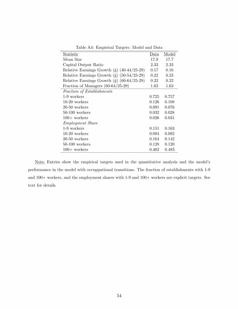
Table A4: Empirical Targets: Model and Data

Statistic Data ModelMean Size 17.9 17.7Capital Output Ratio 2.33 2.33Relative Earnings Growth (g) (40-44/25-29) 0.17 0.16Relative Earnings Growth (g) (50-54/25-29) 0.22 0.23Relative Earnings Growth (g) (60-64/25-29) 0.22 0.22Fraction of Managers (60-64/25-29) 1.63 1.63Fraction of Establishments1-9 workers 0.725 0.75710-20 workers 0.126 0.10820-50 workers 0.091 0.07650-100 workers 0.032 0.028100+ workers 0.026 0.031Employment Share1-9 workers 0.151 0.16310-20 workers 0.094 0.09220-50 workers 0.164 0.14250-100 workers 0.128 0.120100+ workers 0.462 0.483

Note: Entries show the empirical targets used in the quantitative analysis and the model’s

performance in the model with occuppational transitions. The fraction of establishments with 1-9

and 100+ workers, and the employment shares with 1-9 and 100+ workers are explicit targets. See

text for details.

54

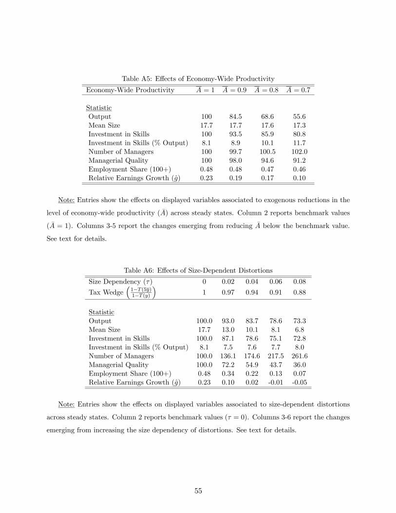
Table A5: Effects of Economy-Wide Productivity

Economy-Wide Productivity A = 1 A = 0.9 A = 0.8 A = 0.7

StatisticOutput 100 84.5 68.6 55.6Mean Size 17.7 17.7 17.6 17.3Investment in Skills 100 93.5 85.9 80.8Investment in Skills (% Output) 8.1 8.9 10.1 11.7Number of Managers 100 99.7 100.5 102.0Managerial Quality 100 98.0 94.6 91.2Employment Share (100+) 0.48 0.48 0.47 0.46Relative Earnings Growth (g) 0.23 0.19 0.17 0.10

Note: Entries show the effects on displayed variables associated to exogenous reductions in the

level of economy-wide productivity (A) across steady states. Column 2 reports benchmark values

(A = 1). Columns 3-5 report the changes emerging from reducing A below the benchmark value.

See text for details.

Table A6: Effects of Size-Dependent Distortions

Size Dependency (τ) 0 0.02 0.04 0.06 0.08

Tax Wedge(1−T (5y)1−T (y)

)1 0.97 0.94 0.91 0.88

StatisticOutput 100.0 93.0 83.7 78.6 73.3Mean Size 17.7 13.0 10.1 8.1 6.8Investment in Skills 100.0 87.1 78.6 75.1 72.8Investment in Skills (% Output) 8.1 7.5 7.6 7.7 8.0Number of Managers 100.0 136.1 174.6 217.5 261.6Managerial Quality 100.0 72.2 54.9 43.7 36.0Employment Share (100+) 0.48 0.34 0.22 0.13 0.07Relative Earnings Growth (g) 0.23 0.10 0.02 -0.01 -0.05

Note: Entries show the effects on displayed variables associated to size-dependent distortions

across steady states. Column 2 reports benchmark values (τ = 0). Columns 3-6 report the changes

emerging from increasing the size dependency of distortions. See text for details.

55

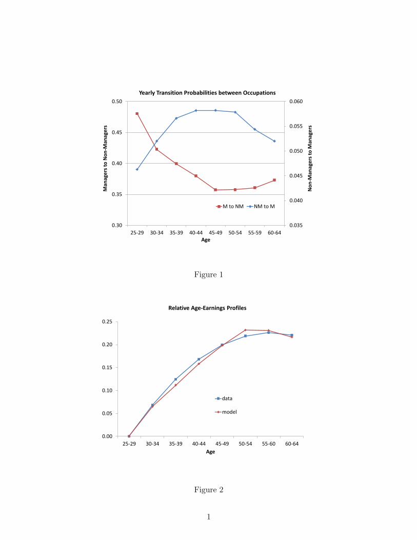
0.035

0.040

0.045

0.050

0.055

0.060

0.30

0.35

0.40

0.45

0.50

25-29 30-34 35-39 40-44 45-49 50-54 55-59 60-64

No

n-M

anag

ers

to

Man

age

rs

Man

age

rs t

o N

on

-Man

age

rs

Age

Yearly Transition Probabilities between Occupations

M to NM NM to M

Figure 1

0.00

0.05

0.10

0.15

0.20

0.25

25-29 30-34 35-39 40-44 45-49 50-54 55-60 60-64

Age

Relative Age-Earnings Profiles

data

model

Figure 2

1