Managerial Hedging, Equity Ownership, and

Firm Value1

Viral V. Acharya

London Business School

and CEPR

Alberto Bisin

New York University

November 20052

1Acharya is at the Institute of Finance and Accounting, London Business School, 6 Sussex Place,Regent’s Park, London - NW1 4SA, United Kingdom. Tel: +44 (0)20 7262 5050 x. 3535. Email:vacharya@london.edu. Acharya is also a Research Affiliate of the Centre for Economic PolicyResearch (CEPR). Bisin is at the Department of Economics, New York University, 269 Mercer St.,New York, NY 10003. Tel: (212) 998 8916. Email: alberto.bisin@nyu.edu.

2This paper was earlier circulated under the titles “Entrepreneurial Incentives in Stock MarketEconomies” and “Managerial Hedging and Equity Ownership.” We thank Phillip Bond, PeterDeMarzo, James Dow, Doug Diamond, Douglas Gale, Pierro Gottardi, Denis Gromb, Eric Hilt,Ravi Jagannathan, Li Jin, Kose John, Martin Lettau, Antonio Mello, Gordon Phillips, AdrianoRampini, Raghu Sundaram, Paul Willen, Luigi Zingales, seminar participants at European FinanceAssociation Meetings 2003, Annual Finance Association Meetings 2004, London Business School,Stern School of Business-NYU, Northwestern University, Universiteit van Amsterdam, Universityof Maryland at College Park, and Washington University-St. Louis for helpful discussions, andNancy Kleinrock for editorial assistance. We are especially grateful to Yakov Amihud for detailedfeedback, to an anonymous referee for comments which have greatly improved the paper, and toHongjun Yan for excellent research assistance. Bisin thanks the C.V. Starr Center for AppliedEconomics for technical and financial support.

Abstract

Managerial Hedging, Equity Ownership, and Firm Value

Risk-averse managers can hedge the aggregate component of their exposure to firm’s cash

flow risk by trading in financial markets, but cannot hedge their firm-specific exposure. This

gives them incentives to load their firm’s cash flows on aggregate risk, that is, to pass up

firm-specific projects in favor of standard projects that contain greater aggregate risk. Such

risk substitution is a form of moral hazard and it gives rise to excessive aggregate risk in

stock markets and excessive correlation of returns across firms and sectors, thereby reducing

the risk-sharing among stock market investors.

A contract specifying managerial equity ownership of the firm can be designed to miti-

gate this moral hazard. We show that the optimal contract might require “negative incentive

compensation,” whereby managerial ownership is smaller than in absence of this moral haz-

ard. We characterize the resulting endogenous relationship between managerial ownership

and (i) the extent of aggregate risk in the firm’s cash flows, as well as (ii) firm value. We show

that these endogenous relationships help explain the shape of the empirically documented

relationship between ownership and firm performance.

Keywords: Managerial Compensation, Diversification, Aggregate Risk, Firm-specific Risk,

Capital Asset Pricing Model (CAPM).

J.E.L. Classification Code: G31, G32, G10, D52, D62, J33.

1 Introduction

Corporate finance theory suggests that managers (and entrepreneurs) receive incentive com-

pensation schemes to align their interests with those of the claimants of their firm. Such

schemes determine the share of their own firm that managers must retain in their portfolios.

Accordingly, these schemes restrict managers from freely trading their firm, and at times

even correlated firms. Similarly, a diverse set of regulations in financial markets also restrict

the ability of managers to trade their own firm’s stock.1 Nonetheless, no regulation restricts

or imposes disclosure on the portfolios of managers in dimensions other than the ownership

of the managed firm. Also, rarely do boards impose direct contractual limitations on man-

agerial hedging, a phenomenon that Schizer (2000) documents on the basis of off-the-record

interviews with investment bankers, and that some authors, most notably, Bebchuk, Fried

and Walker (2002), consider as a manifestation of managerial rent-extraction.

Given the lack of such contractual restrictions, risk-averse managers can (and do) to an

extent enter financial markets in order to privately hedge their risk exposure to the firm.

Evidence of managerial hedging is provided in the law literature by Easterbrook (2002) and

in the finance literature by Bettis, Bizjak, and Lemmon (2001). Recent empirical evidence

shows however that managers appear to be able to hedge aggregate-risk exposure more

effectively than firm-specific risk. For instance, Jin (2002) and Garvey and Milbourn (2002)

find that the pay-performance sensitivity of incentive contracts falls with the idiosyncratic

risk of firm’s cash flows but is invariant to the market risk. This finding is consistent with

managers hedging their aggregate-risk exposure, for example, by trading in market indices

or basket products, but being restricted from trading in their own firms.

If the restrictions imposed on managers’ trading in financial markets principally concerns

trading in their own firms (as we argued above), then risk-averse managers have an incentive

to substitute the unhedgeable, firm-specific risk of their firm’s cash flows for hedgeable,

aggregate risks. For example, they may pass up innovative projects with firm-specific risk in

favor of standard projects that have greater aggregate risk. Such risk-substitution enables

managers to be better diversified, but has perverse implications for aggregate risk-sharing in a

general equilibrium context: If all managers in the economy engage in such risk substitution,

then the correlation of cash flows of different firms is enhanced, as is, in turn, the aggregate

risk in stock markets.

This form of moral hazard induced by incentive compensation, specifically, the substi-

1Since 1994, in the United States such trades must be disclosed to the Securities and Exchange Commis-sion. Disclosure rules regarding own stock trading have also become stricter with the Sarbanes-Oxley Actof 2002. Furthermore, additional regulation is often imposed by the law of firm’s state of incorporation, bythe rules of stock exchange where the firm is listed, and by the firm’s articles of incorporation.

1

tution from unhedgeable, firm-specific risk in firm’s cash flows toward hedgeable aggregate

risks, has not been directly studied. Theoretical and empirical literature in corporate finance

has concentrated instead on the incentives of managers to inefficiently alter only the firm-

specific variance by means of diversification activities (Amihud and Lev, 1981, and Lambert,

1986), or to reduce firm’s expected cash flow by expropriation of firm’s assets and diversion

of cash flow (Jensen, 1986).

We cast our risk-substitution moral hazard in a general-equilibrium setting in order to

address the efficiency of endogenous risk composition. We show that in equilibrium, the

level of aggregate risk in the stock market exceeds the first-best level. Nonetheless, it is

constrained (second-best) efficient. We study the positive aspects of this moral hazard

by characterizing the optimal contract designed to address it. We show that the optimal

contract might require “negative incentive compensation,” whereby managerial ownership

is smaller than in absence of the risk-substitution moral hazard.2 We also characterize the

resulting equilibrium relationship between managerial equity ownership and (i) the extent of

aggregate risk in the firm’s cash flows, as well as (ii) firm’s performance as measured by firm

value. This analysis provides a structural model of the relationships between managerial

ownership, risk composition, expected returns, and firm value, and has important empirical

implications. In particular, we show that these endogenous relationships help explain various

important cross-sectional relationships documented in corporate finance.

A detailed summary of our analysis follows. We study firms in an incomplete-markets,

general-equilibrium Capital Asset Pricing Model (CAPM) economy. The fraction of their

firm that managers and entrepreneurs retain in their portfolios, i.e., their equity ownership of

the firm, is determined contractually. Contractual agreements cannot, however, restrict their

trades in aggregate indexes. Once the ownership structure of firms is designed, agents trade

in financial markets and prices are determined. Subsequently, entrepreneurs and managers

choose the technology of the firm. Firms can produce a given expected cash flow with a given

total risk through the use of different technologies: Some technologies are standard and have

greater betas with respect to the aggregate risk factor and thus have greater aggregate risk;

others are innovative and have lower betas with respect to the aggregate risk factor and thus

have greater firm-specific risk. Technological innovation (modifying the ‘intrinsic’ or the

initial aggregate risk beta of each firm’s project) is costly for entrepreneurs and managers.

The resulting aggregate risk beta is not observed by the firm’s investors.

The choice of the firm’s technology introduces moral hazard. In equilibrium, managers

2To be precise, our intended interpretation of the phrase “negative incentive compensation” is as “neg-ative” incentive-compensation rather than as “negative-incentive” compensation. In other words, the levelof managerial ownership is smaller than that under the first-best, and not such that it provides (negative)incentives to destroy firm value.

2

retain a positive share of their own firm in their portfolios. But, because they are risk-

averse and they can hedge only the aggregate risk exposure by trading in market indexes,

managers have an incentive to increase the aggregate risk beta of their firm’s cash flows: By

loading their firm’s projects on aggregate risk, managers can reduce their own exposure to

unhedgeable firm-specific risks. Such risk-substitution by managers aimed at diversification

of their personal portfolios occurs at the cost of reducing the firm’s market value: under

CAPM pricing, the market price of the firm’s shares decreases in its aggregate risk beta, for

given mean and variance of its cash flow.

We characterize the optimal ownership structure of firms in the face of such moral hazard

and the induced equilibrium risk composition of firms’ cash flows. We show that if the

firm’s technology is intrinsically more loaded on aggregate risk factors (for example, in pro-

cyclical industries), then the optimal ownership scheme provides managers with a lower

equity holding of their firms. The risk-substitution moral hazard is particularly severe for

firms with high intrinsic aggregate risk loadings. Thus, in equilibrium, a smaller managerial

ownership share is optimal for these firms. Indeed, it may even be optimal for these firms to

choose equity holdings for managers that are smaller than the optimal contractual holdings

in absence of moral hazard, a form of “negative incentive compensation.”

Our analysis has rich empirical implications. First, firms whose entrepreneurs or man-

agers hold a larger share of equity in equilibrium are characterized by less aggregate risk in

equilibrium, and hence by low expected returns. This implies, other things being equal, a

negative relationship between managerial ownership and expected returns. To our knowl-

edge, such a relationship has yet to be explored empirically.

Second, the risk-substitution moral hazard we study, when combined with an alternate

moral hazard, for example, Jensen (1986)’s free cash-flow agency problem, can help explain

the hump-shaped cross-sectional relationship between managerial ownership and firm per-

formance, measured by the ratio of the firm’s market value to book value (documented by

Morck, Shleifer, and Vishny, 1988, and McConnell and Servaes, 1990, among others). In

particular, all else being equal, as the risk-substitution moral hazard becomes more severe, a

positive equilibrium relationship is obtained between managerial ownership and performance.

In contrast, an increase in the severity of the free cash-flow problem induces a negative rela-

tionship between ownership and performance (as also found empirically by Bizjak, Brickley

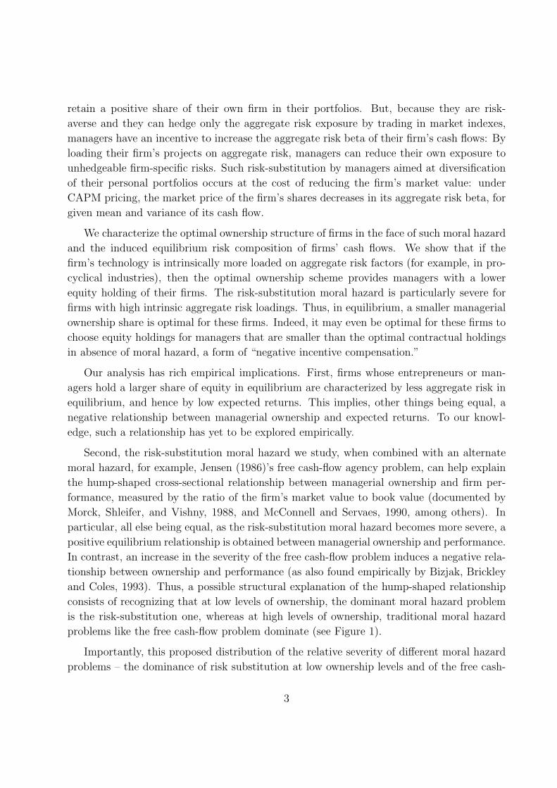
and Coles, 1993). Thus, a possible structural explanation of the hump-shaped relationship

consists of recognizing that at low levels of ownership, the dominant moral hazard problem

is the risk-substitution one, whereas at high levels of ownership, traditional moral hazard

problems like the free cash-flow problem dominate (see Figure 1).

Importantly, this proposed distribution of the relative severity of different moral hazard

problems – the dominance of risk substitution at low ownership levels and of the free cash-

3

flow problem at high ownership levels – has independent implications regarding the shape

of the relationship between managerial ownership and diversification. In particular, since

risk substitution implies a negative relationship between ownership and diversification, and

the free cash-flow problem a positive one, the proposed distribution implies a U-shaped

relationship between diversification and ownership. This is in fact what Denis, Denis, and

Sarin (1997) find, measuring diversification as the R2 in a regression of firm’s stock returns

on market returns. We interpret this as evidence that our analysis of the risk-substitution

moral hazard has the potential to simultaneously explain, as equilibrium relationships, the

hump-shaped relationship between firm performance and inside ownership, and the U-shaped

relationship between diversification (R2) and inside ownership.

The choice of risk composition of firms’ cash flows by managers also endogenously affects

the level of risk-sharing in the economy. We show that, in equilibrium, managers choose

aggregate risk in their firm’s cash flows that exceeds the first-best level. However, market

prices and the optimal ownership structure of the firm induce a level of aggregate risk in firms

that is constrained (second-best) efficient.3 That is, the ownership structure is efficient from

the point of view of a planner who cannot internalize the externality of managerial activity

aimed at substituting firm-specific risk of firm’s cash flows with aggregate risk. Prices in

financial markets are not only market clearing, but they also efficiently align the objectives

of management and stockholders with those of the constrained social planner: Managers

recognize that increasing the aggregate risk of the firm reduces the equilibrium price of the

firm’s shares; and, in equilibrium, the fraction of the firm’s shares that managers retain

induces them to choose the constrained-efficient firm loadings.

We extend our analysis by considering multiple sectors, whereby the aggregate risk factor

can be interpreted as a stock market index. In this setting, we argue that the risk-substitution

moral hazard also gives rise to an excessive loading of the firm’s stock returns on the index

returns, and, in turn, that it generates an excessive correlation of returns across sectors.

Next, we show that the risk-substitution moral hazard is more severe the greater the extent

of purely idiosyncratic risk in the firm’s cash flows. Finally, we consider the welfare effects

of financial innovations that alter the hedging capability of managers.

Related Literature: The design of entrepreneurial ownership and managerial compensa-

tion under asymmetric information and moral hazard has been examined extensively in the

corporate finance literature. Diamond and Verrechia (1982) and Ramakrishnan and Thakor

(1984) were the first to analyze moral hazard when the firm returns have systematic and

idiosyncratic risks. These papers are cast in partial-equilibrium settings. Our principal the-

3At the first-best, the social planner can choose both the technology of firms and their ownership structure.In contrast, at the second-best the social planner designs the firm’s ownership structure, but must letmanagers and entrepreneurs make technology decisions.

4

oretical contribution is rather to embed the agency-theoretic approach of Fama and Miller

(1972) and Jensen and Meckling (1976) into a general equilibrium model of the price of risk,

such as the CAPM.4

Few general equilibrium analyses of the ownership structure of firms have been developed.

Allen and Gale (1988, 1991) study the capital structure of firms in general equilibrium.

However, they do not study economies with moral hazard. Magill and Quinzii (2002) and

Ou-Yang (2002) do in fact consider the issue of moral hazard between entrepreneurs and

investors in a general equilibrium setting. In the set-up of these papers entrepreneurs can

affect the variance of their firm’s cash flows and/or their levels, rather than their correlation

with aggregate risk, as in our case.

Our structural modeling approach is in the spirit of important antecedents such as Dem-

setz and Lehn (1985), and, more recently, Himmelberg, Hubbard and Love (2002). Specifi-

cally, from the standpoint of providing a structural model linking managerial ownership and

firm value, our paper is closest to the recent work of Coles, Lemmon, and Menschke (2003).

These authors provide a different structural explanation of the hump-shaped empirical rela-

tionship between ownership and performance. We discuss the relationship of our analysis to

theirs in Section 4.

The remainder of the paper is structured as follows. Sections 2 and 3 contain the model

and analysis of the risk-substitution moral hazard. Section 4 discusses empirical implications

and Section 5 addresses the efficiency of equilibrium choices. Section 6 establishes the iso-

morphism between owner-managed firms and corporations. Sections 7 and 8 consider various

extensions. Section 9 concludes. Appendices A–C contain the closed-form expressions for

the competitive equilibrium, the expression for welfare criterion, and the proofs, respectively.

2 The Model

We study a perfectly competitive two-period equilibrium economy in which the CAPM pric-

ing rule can be derived.

A subset of the agents in the economy, entrepreneurs and managers, make capital bud-

geting choices: At a private cost, they can choose their firm’s technology and affect the

risk composition of cash flows and, hence, stock returns. The CAPM setting enables us to

cast the capital budgeting choice faced by entrepreneurs and managers in terms of a choice

4In particular, we follow Willen (1997) in introducing incomplete financial markets and restricted partic-ipation in the CAPM economy. In addition, we introduce assets in positive net supply to capture a stockmarket economy.

5

of betas (i.e., the loadings of cash flows) onto traded risk factors: By choosing the betas

of firm cash flows, entrepreneurs and managers determine the proportion of aggregate and

firm-specific components in the total cash flow risk of firms.

Capital budgeting choices are affected by the equity ownership structure of the firms. To

start with, we assume that entrepreneurs and managers are prohibited from trading the stock

of their own firms and others in the same sector, but they can trade other financial assets.

This endows entrepreneurs and managers with a preference to substitute projects whose cash

flow risk cannot be hedged easily with projects whose cash flow risk is readily hedgeable by

trading in financial markets. This creates the possibility of there being a risk-substitution

moral hazard in the capital budgeting choices of entrepreneurs and managers.

The ownership structure is, in turn, the result of an optimal-contracting problem be-

tween entrepreneurs and investors, or between managers and stockholders. We consider

different corporate governance structures and the contracting problems induced under these

structures. A governance structure determines whether the firm is originally held by entre-

preneurs, as in owner-managed firms, or by stockholders, as in corporations. In the case of

a corporation, the firm is run by managers, that is, the firm is management-controlled. We

concentrate on owner-managed firms for most of the paper. We show in Section 6 that our

results extend isomorphically to corporations.

An owner-managed firm is owned ex-ante by an entrepreneur. If the firm’s cash flow betas

are observable and the entrepreneur can credibly commit to a choice of these betas when

the firm is sold in the stock market, then no moral-hazard concerns arise. Consequently, the

entrepreneur’s choice of ownership structure and the cash flow betas are both optimal. If

instead the cash flow betas are not observed by the market (i.e., they are private information

of the entrepreneur) and the choice of these betas occurs after the firm is sold in the stock

market, then the issue of moral hazard arises.5 In this case, the proportion of the firm that

the entrepreneur retains determines the choice of the firm’s cash flow betas. Investors in the

market rationally anticipate the mapping between the entrepreneur’s holding of the firm and

the choice of betas. Thus, the market price of shares depends upon the publicly observed

ownership structure of the firm. Entrepreneurs also realize that the firm’s value will depend

on its ownership structure, understanding that discounted prices will be associated with

ownership structures that impart incentives to increase the aggregate risk of cash flows.

We introduce formally the simplest version of the model with a representative firm,

5The difficulty in estimating firm’s stock-return betas is ubiquitous in corporate finance and asset pricing,and in fact, is the primary reason for the portfolio-based approach to tests involving firm betas. Hence, it isreasonable to assume that firm’s cash-flow betas are also not perfectly observed by investors. The literaturestarting with Amihud and Lev (1981), that focuses on the alteration of firm-specific risk only, also tacitlyassumes that either the firm’s volatility or its betas are not perfectly observed by shareholders.

6

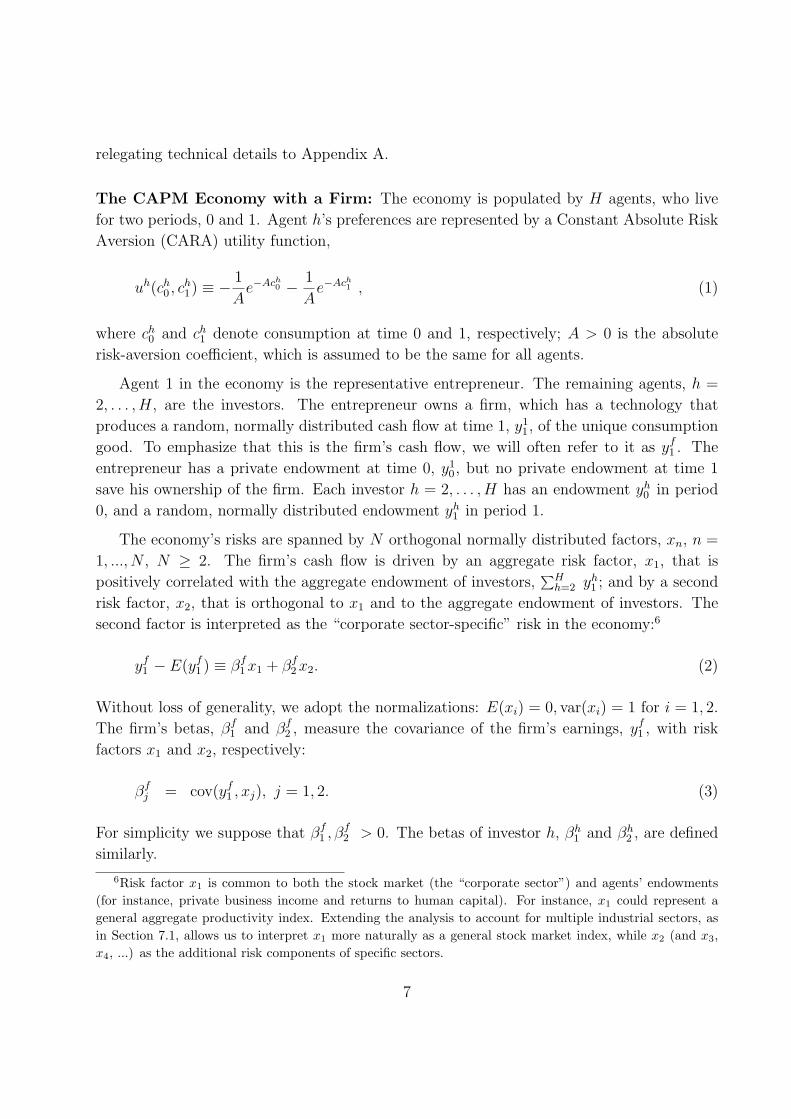
relegating technical details to Appendix A.

The CAPM Economy with a Firm: The economy is populated by H agents, who live

for two periods, 0 and 1. Agent h’s preferences are represented by a Constant Absolute Risk

Aversion (CARA) utility function,

uh(ch0 , c

h1) ≡ −

1

Ae−Ach

0 − 1

Ae−Ach

1 , (1)

where ch0 and ch

1 denote consumption at time 0 and 1, respectively; A > 0 is the absolute

risk-aversion coefficient, which is assumed to be the same for all agents.

Agent 1 in the economy is the representative entrepreneur. The remaining agents, h =

2, . . . , H, are the investors. The entrepreneur owns a firm, which has a technology that

produces a random, normally distributed cash flow at time 1, y11, of the unique consumption

good. To emphasize that this is the firm’s cash flow, we will often refer to it as yf1 . The

entrepreneur has a private endowment at time 0, y10, but no private endowment at time 1

save his ownership of the firm. Each investor h = 2, . . . , H has an endowment yh0 in period

0, and a random, normally distributed endowment yh1 in period 1.

The economy’s risks are spanned by N orthogonal normally distributed factors, xn, n =

1, ..., N , N ≥ 2. The firm’s cash flow is driven by an aggregate risk factor, x1, that is

positively correlated with the aggregate endowment of investors,∑H

h=2 yh1 ; and by a second

risk factor, x2, that is orthogonal to x1 and to the aggregate endowment of investors. The

second factor is interpreted as the “corporate sector-specific” risk in the economy:6

yf1 − E(yf

1 ) ≡ βf1 x1 + βf

2 x2. (2)

Without loss of generality, we adopt the normalizations: E(xi) = 0, var(xi) = 1 for i = 1, 2.

The firm’s betas, βf1 and βf

2 , measure the covariance of the firm’s earnings, yf1 , with risk

factors x1 and x2, respectively:

βfj = cov(yf

1 , xj), j = 1, 2. (3)

For simplicity we suppose that βf1 , βf

2 > 0. The betas of investor h, βh1 and βh

2 , are defined

similarly.

6Risk factor x1 is common to both the stock market (the “corporate sector”) and agents’ endowments(for instance, private business income and returns to human capital). For instance, x1 could represent ageneral aggregate productivity index. Extending the analysis to account for multiple industrial sectors, asin Section 7.1, allows us to interpret x1 more naturally as a general stock market index, while x2 (and x3,x4, ...) as the additional risk components of specific sectors.

7

There are three financial markets: a riskless bond market, where asset 0 with determin-

istic payoff of 1 is traded, a market where the aggregate factor x1 is directly traded, and the

stock market where shares of the representative firm f are traded. The bond and the asset

paying off the aggregate factor x1 are in zero net supply. The fraction w of the firm sold in

the stock market constitutes the positive supply of the stock. The remaining fraction (1−w)

constitutes the equity ownership of the entrepreneur. If an N–dimensional factor structure

drives risk where N > 2, then the economy is one of incomplete markets. Trading in financial

and stock markets is restricted. In particular, we assume that the entrepreneur, after having

placed w shares on the market, cannot trade the stock of his own firm.7 However, all agents

can trade the riskless bond.

We treat the entrepreneur as a price-taker and the economy as competitive. In particular,

we abstract from the ability of entrepreneurs to strategically affect the equilibrium prices.

One can interpret the representative entrepreneur as one of a continuum of entrepreneurs.

Furthermore, for ease of exposition, we assume a firm’s cash flows are driven only by the

aggregate and the corporate sector-specific risk factors, and not by any firm-specific risk

factor. That is, we treat the representative firm as equivalent to the ‘corporate sector’

comprised of a continuum of identical firms. In Section 7.2, we distinguish between the firm

and the sector by allowing the cash flows of each firm to contain both a sector-specific and

a purely firm-specific risk factor. Crucial in these contexts is that either the entrepreneur

cannot hedge his sector-specific risk in financial markets (in the model we analyze below),

or else he cannot hedge his firm-specific risk (in Section 7.2).

2.1 Equilibrium

Our analysis proceeds recursively. First, given arbitrary equity ownership structures and cash

flow betas on risk factors, we solve for the market equilibrium and induced CAPM pricing

rule. Then, given the ownership structure, we analyze the capital budgeting problem, i.e.,

the entrepreneur’s choice of betas. Finally, we study the optimal-contracting problem, which

determines the ownership structure of the firm.

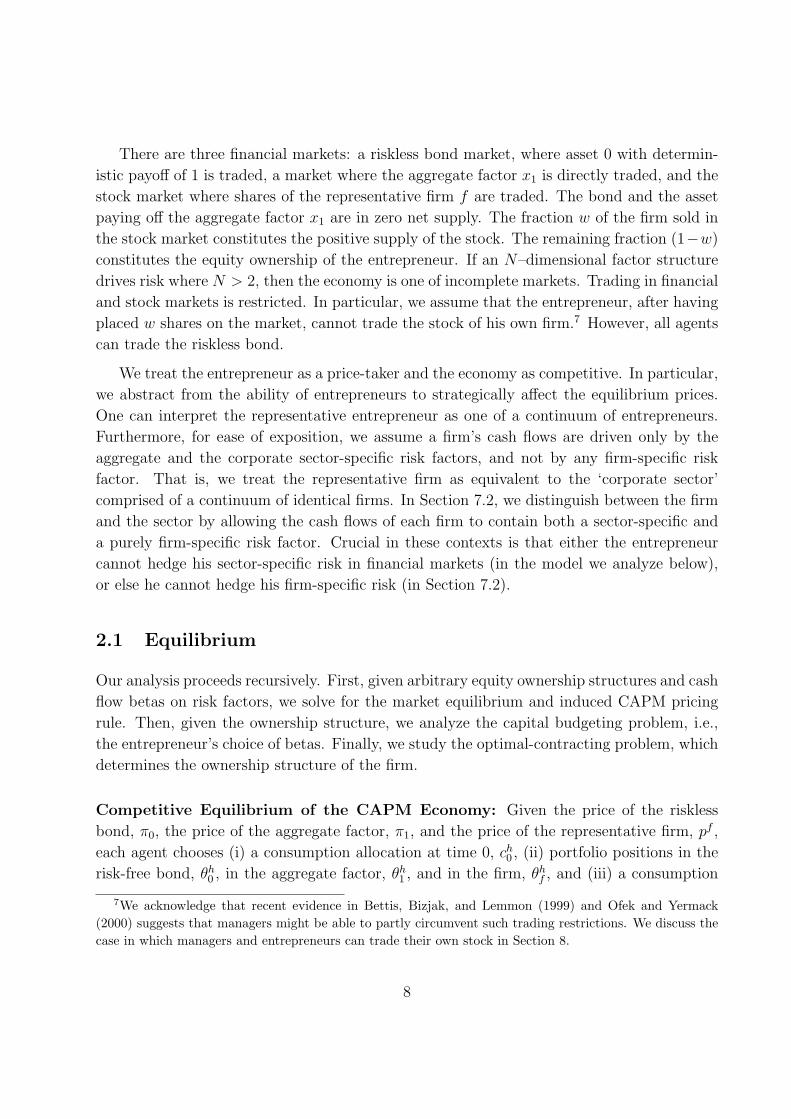
Competitive Equilibrium of the CAPM Economy: Given the price of the riskless

bond, π0, the price of the aggregate factor, π1, and the price of the representative firm, pf ,

each agent chooses (i) a consumption allocation at time 0, ch0 , (ii) portfolio positions in the

risk-free bond, θh0 , in the aggregate factor, θh

1 , and in the firm, θhf , and (iii) a consumption

7We acknowledge that recent evidence in Bettis, Bizjak, and Lemmon (1999) and Ofek and Yermack(2000) suggests that managers might be able to partly circumvent such trading restrictions. We discuss thecase in which managers and entrepreneurs can trade their own stock in Section 8.

8

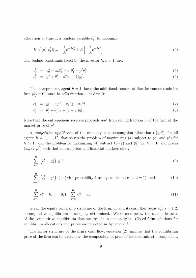
allocation at time 1, a random variable ch1 , to maximize

E[uh(ch0 , c

h1)] ≡ −

1

Ae−Ach

0 + E[− 1

Ae−Ach

1

]. (4)

The budget constraints faced by the investor h, h > 1, are:

ch0 = yh

0 − π0θh0 − π1θ

h1 − pfθh

f (5)

ch1 = yh

1 + θh0 + θh

1x1 + θhfyf

1 . (6)

The entrepreneur, agent h = 1, faces the additional constraint that he cannot trade his

firm (θ1f ≡ 0), once he sells fraction w at date 0:

c10 = y1

0 + wpf − π0θ10 − π1θ

11 (7)

c11 = θ1

0 + θ11x1 + (1− w)yf

1 . (8)

Note that the entrepreneur receives proceeds wpf from selling fraction w of the firm at the

market price of pf .

A competitive equilibrium of the economy is a consumption allocation (ch0 , c

h1), for all

agents h = 1, . . . , H, that solves the problem of maximizing (4) subject to (5) and (6) for

h > 1, and the problem of maximizing (4) subject to (7) and (8) for h = 1; and prices

(π0, π1, pf ) such that consumption and financial markets clear:

H∑h=1

(ch0 − yh

0

)≤ 0, (9)

H∑h=1

(ch1 − yh

1

)≤ 0 (with probability 1 over possible states at t = 1), and (10)

H∑h=1

θhj = 0, j = 0, 1;

H∑h=2

θhf = w. (11)

Given the equity ownership structure of the firm, w, and its cash flow betas βfj , j = 1, 2,

a competitive equilibrium is uniquely determined. We discuss below the salient features

of the competitive equilibrium that we exploit in our analysis. Closed-form solutions for

equilibrium allocations and prices are reported in Appendix A.

The factor structure of the firm’s cash flow, equation (2), implies that the equilibrium

price of the firm can be written as the composition of price of the deterministic component,

9

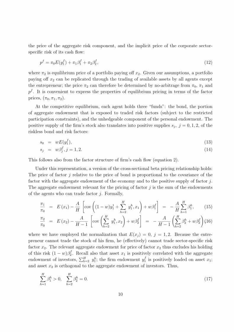
the price of the aggregate risk component, and the implicit price of the corporate sector-

specific risk of its cash flow:

pf = π0E(yf1 ) + π1β

f1 + π2β

f2 , (12)

where π2 is equilibrium price of a portfolio paying off x2. Given our assumptions, a portfolio

paying off x2 can be replicated through the trading of available assets by all agents except

the entrepreneur; the price π2 can therefore be determined by no-arbitrage from π0, π1 and

pf . It is convenient to express the properties of equilibrium pricing in terms of the factor

prices, (π0, π1, π2).

At the competitive equilibrium, each agent holds three “funds”: the bond, the portion

of aggregate endowment that is exposed to traded risk factors (subject to the restricted

participation constraints), and the unhedgeable component of the personal endowment. The

positive supply of the firm’s stock also translates into positive supplies sj, j = 0, 1, 2, of the

riskless bond and risk factors:

s0 = wE(yf1 ), (13)

sj = wβfj , j = 1, 2. (14)

This follows also from the factor structure of firm’s cash flow (equation 2).

Under this representation, a version of the cross-sectional beta pricing relationship holds:

The price of factor j relative to the price of bond is proportional to the covariance of the

factor with the aggregate endowment of the economy and to the positive supply of factor j.

The aggregate endowment relevant for the pricing of factor j is the sum of the endowments

of the agents who can trade factor j. Formally,

π1

π0

= E (x1)−A

H

[cov

((1− w)y1

1 +H∑

h=2

yh1 , x1

)+ wβf

1

]= − A

H

H∑h=1

βh1 , (15)

π2

π0

= E (x2)−A

H − 1

[cov

(H∑

h=2

yh1 , x2

)+ wβf

2

]= − A

H − 1

(H∑

h=2

βh2 + wβf

2

),(16)

where we have employed the normalization that E(xj) = 0, j = 1, 2. Because the entre-

preneur cannot trade the stock of his firm, he (effectively) cannot trade sector-specific risk

factor x2. The relevant aggregate endowment for price of factor x2 thus excludes his holding

of this risk (1 − w)βf2 . Recall also that asset x1 is positively correlated with the aggregate

endowment of investors,∑H

h=2 yh1 ; the firm endowment yf

1 is positively loaded on asset x1;

and asset x2 is orthogonal to the aggregate endowment of investors. Thus,

H∑h=1

βh1 > 0,

H∑h=2

βh2 = 0. (17)

10

Finally, in equilibrium, the expected utility of agent h is

E[uh(ch0 , c

h1)] = −(1 + π0)

Ae−Ach

0 (w,βf1 ,βf

2 ,pf ) , (18)

where we stress the fact that the equilibrium time-0 consumption depends on the ownership

structure of the firm, its technology, and the price of the firm. This expected utility also

depends on the induced equilibrium prices, (πj), j = 0, 1, 2, that we omit for parsimony.

2.2 Capital Budgeting and Equity Ownership Structure

The entrepreneur can, at a private non-pecuniary cost, choose the the risk composition of the

firm’s cash flows. Formally, the entrepreneur can choose the betas, βf1 and βf

2 , the respective

loadings of the firm’s cash flows on the aggregate risk and the corporate sector-specific

risk.8 For simplicity, we assume the entrepreneur’s choice only affects the distribution of

the variance of cash flows between the aggregate and the sector-specific risks, but does not

alter their expected value or the total variance. That is, the entrepreneur’s choice consists of

substituting between projects which are innovative and projects that are otherwise identical

but are standard and more exposed to aggregate risk.9 That is, we assume that

(βf1 )2 + (βf

2 )2 = V , (19)

where V , the total variance of the cash flow of the firm, is held constant.

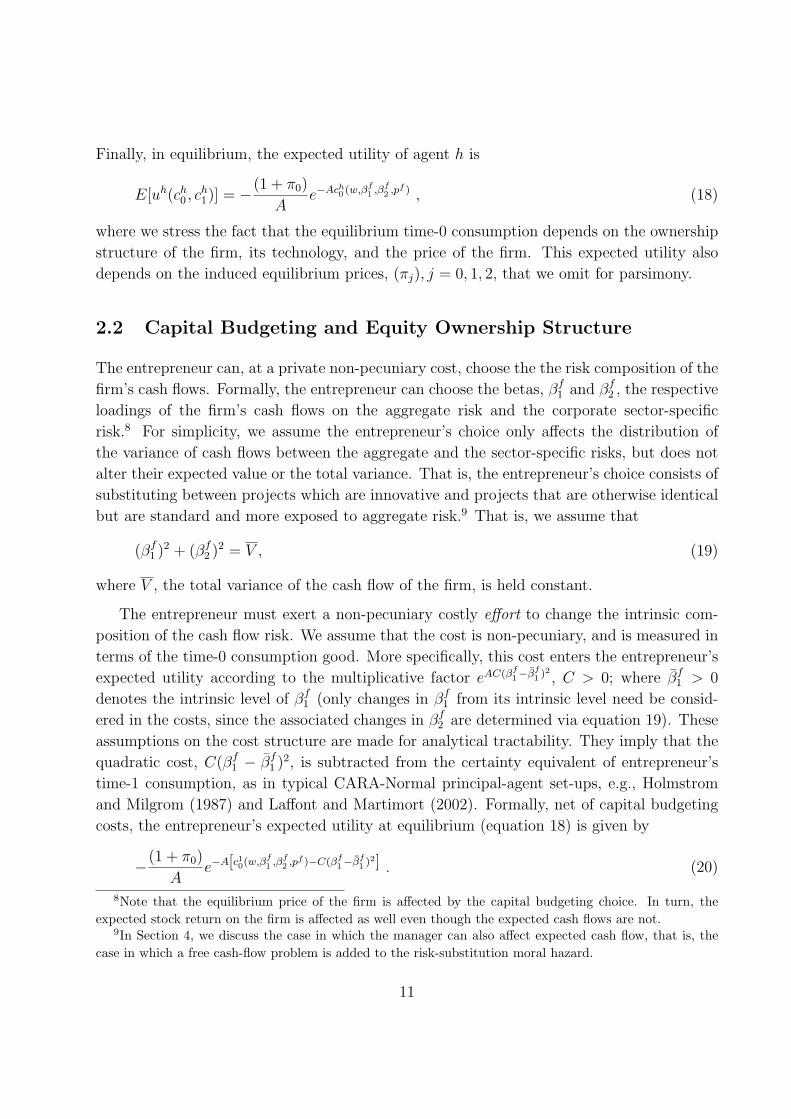
The entrepreneur must exert a non-pecuniary costly effort to change the intrinsic com-

position of the cash flow risk. We assume that the cost is non-pecuniary, and is measured in

terms of the time-0 consumption good. More specifically, this cost enters the entrepreneur’s

expected utility according to the multiplicative factor eAC(βf1−βf

1 )2 , C > 0; where βf1 > 0

denotes the intrinsic level of βf1 (only changes in βf

1 from its intrinsic level need be consid-

ered in the costs, since the associated changes in βf2 are determined via equation 19). These

assumptions on the cost structure are made for analytical tractability. They imply that the

quadratic cost, C(βf1 − βf

1 )2, is subtracted from the certainty equivalent of entrepreneur’s

time-1 consumption, as in typical CARA-Normal principal-agent set-ups, e.g., Holmstrom

and Milgrom (1987) and Laffont and Martimort (2002). Formally, net of capital budgeting

costs, the entrepreneur’s expected utility at equilibrium (equation 18) is given by

−(1 + π0)

Ae−A[c10(w,βf

1 ,βf2 ,pf )−C(βf

1−βf1 )2] . (20)

8Note that the equilibrium price of the firm is affected by the capital budgeting choice. In turn, theexpected stock return on the firm is affected as well even though the expected cash flows are not.

9In Section 4, we discuss the case in which the manager can also affect expected cash flow, that is, thecase in which a free cash-flow problem is added to the risk-substitution moral hazard.

11

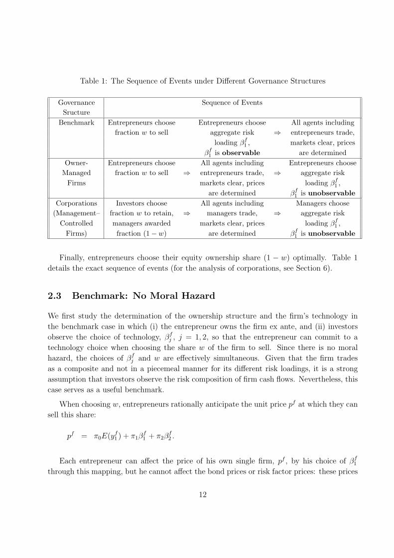
Table 1: The Sequence of Events under Different Governance Structures

Governance Sequence of EventsSructure

Benchmark Entrepreneurs choose Entrepreneurs choose All agents includingfraction w to sell aggregate risk ⇒ entrepreneurs trade,

loading βf1 , markets clear, prices

βf1 is observable are determined

Owner- Entrepreneurs choose All agents including Entrepreneurs chooseManaged fraction w to sell ⇒ entrepreneurs trade, ⇒ aggregate risk

Firms markets clear, prices loading βf1 ,

are determined βf1 is unobservable

Corporations Investors choose All agents including Managers choose(Management– fraction w to retain, ⇒ managers trade, ⇒ aggregate risk

Controlled managers awarded markets clear, prices loading βf1 ,

Firms) fraction (1− w) are determined βf1 is unobservable

Finally, entrepreneurs choose their equity ownership share (1 − w) optimally. Table 1

details the exact sequence of events (for the analysis of corporations, see Section 6).

2.3 Benchmark: No Moral Hazard

We first study the determination of the ownership structure and the firm’s technology in

the benchmark case in which (i) the entrepreneur owns the firm ex ante, and (ii) investors

observe the choice of technology, βfj , j = 1, 2, so that the entrepreneur can commit to a

technology choice when choosing the share w of the firm to sell. Since there is no moral

hazard, the choices of βfj and w are effectively simultaneous. Given that the firm trades

as a composite and not in a piecemeal manner for its different risk loadings, it is a strong

assumption that investors observe the risk composition of firm cash flows. Nevertheless, this

case serves as a useful benchmark.

When choosing w, entrepreneurs rationally anticipate the unit price pf at which they can

sell this share:

pf = π0E(yf1 ) + π1β

f1 + π2β

f2 .

Each entrepreneur can affect the price of his own single firm, pf , by his choice of βf1

through this mapping, but he cannot affect the bond prices or risk factor prices: these prices

12

are determined at equilibrium by the aggregate choices of the continuum of entrepreneurs.

That is, markets are competitive, and all agents including entrepreneurs are price takers:

All agents rationally anticipate that the price of a single firm depends on its cash flow betas

βfj , given the prices of traded assets in the economy.10

Formally, the representative entrepreneur chooses the share w of the firm to sell, as well

as its technology βf1 to maximize expected utility net of the exerted effort:

maxw,βf1 ,βf

2− (1+π0)

Ae−A[c10(w,βf

1 ,βf2 ,pf )−C(βf

1−βf1 )2] (21)

subject to:

pf = π0E(yf1 ) + π1β

f1 + π2β

f2 , (22)

(βf1 )2 + (βf

2 )2 = V , (23)

given the equilibrium prices of the bond and the risk factors, π0, π1, and π2, respectively.

2.4 Moral Hazard

In contrast to this benchmark case, consider now owner-managed firms where the technology

choice is not observed by capital market investors. As a result, entrepreneurs cannot commit

their technology choice, βfj , at the moment they choose the fraction w of their firm to sell in

the market; they choose βfj after they choose w, and after agents have traded and markets

have cleared. While the specific timing of the choice of βfj and trading in capital markets

is somewhat arbitrary, crucial for our analysis is that the chosen βfj are not observed by

investors in competitive markets.

Proceeding recursively, we first study the capital budgeting problem of entrepreneurs,

which determines βfj for a given w. Since w is observed by investors, but βf

j is not, entrepre-

neurs anticipate that the price of their own firm pf will depend only on w and not on their

specific choice of βfj . Therefore, for given w and pf , the choice of cash flow betas maximizes

the entrepreneur’s expected utility net of the exerted effort:

maxβf1 ,βf

2− (1+π0)

Ae−A[c10(w,βf

1 ,βf2 ,pf )−C(βf

1−βf1 )2] (24)

10As discussed in Section 2 and assumed in Section 2.1, the entrepreneur takes as given the price of theriskless bond, π0, the price of the aggregate risk factor, π1, and the price of the representative firm, pf . Thecomposition of pf , equation (12), implies that, in addition to π0 and π1, the entpreneur effectively takes asgiven the price of the sector-specific risk factor, π2.

The price of entrepreneur’s own firm is also denoted as pf for parsimony of notation. The entrepreneurrecognizes that this price depends on the risk composition of his firm’s cash flows, for given prices of riskfactors. In equilibrium, the price of each entrepreneur’s firm equals the price of the representative firm.

13

subject to

(βf1 )2 + (βf

2 )2 = V . (25)

Because the price of the firm pf does not affect the solution of this capital budgeting problem,

we denote the solution simply as βfj (w).

We now consider the choice of equity ownership by entrepreneurs. An entrepreneur’s

proceeds from selling share w of his firm are wpf . Hence, he perceives a direct effect of the

choice of w on his proceeds. In addition, the entrepreneur expects investors to rationally

anticipate the equilibrium map between ownership structure and the risk composition of

the firm, βfj (w), which results from the solution of the capital budgeting problem. The

entrepreneur therefore also perceives an indirect effect of his choice of w on the price of the

firm pf (equation 12) through its effect on his future choice of βfj via the map βf

j (w).11

Formally, the entrepreneur chooses w to maximize the expected utility net of effort:

maxw − (1+π0)A

e−A[ch0 (w,βf

1 ,βf2 ,pf )−C(βf

1−βf1 )2] (26)

subject to:

pf = π0E(yf1 ) + π1β

f1 + π2β

f2 , (27)

βfj = βf

j (w), j = 1, 2, (28)

given πj, j = 0, 1, 2.

3 Equilibrium Equity Ownership and Risk

We characterize below (i) the entrepreneurial choice of the aggregate risk beta of the firm’s

cash flows, βf1 ; and (ii) the optimal equity ownership of firms, measured by the fraction

(1−w) retained by entrepreneurs. We first consider the benchmark case when investors can

observe the firm’s risk loadings and hence there is no moral hazard.

11This equilibrium concept is related to the one introduced in the context of general equilibrium theorywith asymmetric information by Prescott and Townsend (1984). The formulation we adopt is however Magilland Quinzii (2002)’s who, in a related setting, explicitly formulate the anticipatory behavior of entrepreneursas “rational conjectures.” Bisin and Gottardi (1999) study a different equilibrium concept appropriate whenthe equity ownership structure is also not observable.

14

Proposition 1 For owner-managed firms with no moral hazard, in equilibrium, the loading

on the aggregate risk factor, denoted β∗1 , is reduced from its initial value βf1 :

β∗1 = βf1 −

Aπ0

2CH(1 + π0)

H∑h=2

βh1 < βf

1 . (29)

Each entrepreneur sells fraction w∗ of the firm, retaining fraction

(1− w∗) =1

H. (30)

In the absence of risk-substitution moral hazard, each entrepreneur simply owns the

market fraction of the firm. The entrepreneur rationally anticipates that increasing the

aggregate risk of the firm, thereby reducing the firm-specific risk, reduces the equilibrium

value of its shares (equation 12). Hence, in equilibrium, the entrepreneur optimally reduces

the aggregate risk loading of the firm, choosing β∗1 < βf1 .

Now consider owner-managed firms when investors do not observe the firm’s risk loadings.

In this case, entrepreneurs do not fully internalize the cost borne by the rest of the economy

due to an increase in their firm’s aggregate risk beta. In particular, entrepreneurs privately

prefer to increase their firm’s aggregate risk beta in order to reduce the fraction of their

own wealth that is composed of unhedgeable risk. However, such risk-substitution is costly

for investors: Investors’ endowments are exposed to aggregate risk, but not to corporate

sector-specific risk. The result is that investors can bear the corporate sector-specific risk

supplied by the stock market at a lower welfare loss than they can bear the aggregate risk.

Entrepreneurs can, however, design the ownership structure to reduce the extent of ineffi-

cient risk substitution, i.e., to create an incentive to decrease the aggregate risk beta of cash

flows. We characterize the equilibrium loading on aggregate risk, βf1 , and also the condition

on the initial loading βf1 that guarantees the equilibrium level of ownership retained by the

entrepreneur is smaller than the market share.

Proposition 2 For owner-managed firms with moral hazard, in equilibrium, the loading on

the aggregate risk factor, β∗∗1 , is such that

β∗1 < β∗∗1 < βf1 . (31)

The fraction of the firm retained by the entrepreneur, (1− w∗∗), is such that

(1− w∗∗) < (1− w∗) (32)

15

if

βf1 > K

H∑h=2

βh1 , where K = 1 +

A

4CH2. (33)

At equilibrium, the optimal choice of w induces entrepreneurs to decrease the aggregate

cash flow beta of their firms, β∗∗1 < βf1 , but not fully to the level without moral hazard,

β∗1 < β∗∗1 . When the intrinsic aggregate risk beta of the firm βf1 is sufficiently high and/or

the aggregate risk beta of investors’ endowments∑H

h=2 βh1 is sufficiently low, condition (33)

is satisfied and entrepreneurs hold a smaller fraction of the firm compared to the benchmark

case, (1− w∗∗) < (1− w∗).

This result is important in the context of our analysis. It demonstrates that, under cer-

tain conditions, the optimal contract designed to mitigate the risk-substitution moral hazard

requires entrepreneurs to hold a smaller fraction of the firm than they would hold if such

moral hazard were not to be present. We interpret this as a sort of “negative incentive

compensation”: ownership can in fact have adverse incentive effects on managers. As a con-

sequence, firms where the risk-substitution problem is most severe, for example, pro-cyclical

firms which intrinsically have high aggregate risk, should optimally design contracts offering

a smaller equity ownership to entrepreneurs. There exists no closed-form characterization

for the equilibrium dependence of equity ownership on the firm’s intrinsic aggregate-risk

loading. Hence, we have confirmed this implication numerically; see Figure 2.

Before we discuss the empirical implications of Proposition 2, we discuss condition (33)

underlying the negative incentive compensation. We present its intuitive interpretation and

discuss its reasonableness from an empirical standpoint.12

On the one hand, entrepreneurs benefit from increasing aggregate risk of firm cash flows

because it reduces their exposure to unhedgeable, firm-specific risk. On the other hand,

entrepreneurs also face a cost from doing so. In equilibrium, entrepreneurs diversify their

personal portfolio by selling the aggregate risk component of their wealth, (1 − w)βf1 , at

the given price π1, and retain only the average market component of this risk, 1H

∑Hh=1 βh

1 .

Since aggregate risk is disliked by agents, it is sold at a negative price and its re-balancing is

costly for entrepreneurs. In other words, the price of supplying aggregate risk to the markets

counteracts the entrepreneurial incentives to increase the aggregate risk of cash flows.

The effectiveness of using ownership structure to pre-commit a reduction in the aggregate

cash flow beta depends upon the relative strengths of these two conflicting effects. The price

of aggregate risk π1 increases (in magnitude) with the aggregate risk beta of investors’

12The formal argument is based on the mixed partial derivative of entrepreneurial objective (equation 24)with respect to the aggregate risk beta of cash flows, βf

1 , and the share retained, (1− w).

16

endowments,∑H

h=2 βh1 . When

∑Hh=2 βh

1 is sufficiently low relative to βf1 , the cost of hedging

aggregate risk is not too high and entrepreneurs can diversify easily by personal trading. In

this case, the only feasible pre-commitment device is one that exposes entrepreneurs to less

unhedgeable risk than in the benchmark case: Entrepreneurial ownership is lower than in

the benchmark case and this itself provides diversification to the entrepreneur.

However, when the aggregate risk exposure of the investors’ endowment∑H

h=2 βh1 is high,

it is costly for entrepreneurs to sell aggregate risk in capital markets. The optimal pre-

commitment device is now one where the entrepreneur retains a fraction of the firm that

exceeds the market share. This induces the entrepreneur to diversify by trading in capital

markets: Since the quantity of aggregate risk the entrepreneur has to sell increases in the

aggregate risk beta of the firm, the entrepreneur is incentivized to choose a smaller aggregate

beta. Formally, a sufficient condition for this case to arise is βf1 <

∑Hh=2 βh

1 .

To better understand condition (33) from an empirical standpoint, suppose that the

aggregate risk factor x1 is perfectly correlated with∑H

h=2 yh1 , the non-corporate sector (in-

vestors’) endowment of the economy. Then, x1 could be interpreted as the Gross Domestic

Product (GDP) minus the corporate sector output, but normalized to have unit variance.

Thus,∑H

h=2 βh1 equals

√V nc, where V nc is the variance of the non-corporate sector en-

dowment. Furthermore, βf1 equals ρ

√V , where V is the variance of the corporate sector

endowment, and ρ is the correlation between corporate sector and non-corporate sector en-

dowments. Finally, let H go to infinity keeping V nc and ρ constant.13 Then, K tends to unity,

and condition (33) requires that ρ2 V > V nc, or in other words, that the correlation of corpo-

rate sector cash flows and non-corporate sector endowments be high and that the variability

of corporate sector cash flows be large relative to the variability of non-corporate sector

endowments. Empirical evidence suggests that the corporate sector output of economies is

highly correlated with the non-corporate sector output, and is much more variable.14

13This can be achieved for example by distributing investors into a continuum of cohorts that are rankedby the correlation of investors’ endowment with corporate sector endowment, the correlations ranging froma minimum negative value to a maximum positive value.

14For example, based on data from the National Income and Product Accounts Table, the de-trendedcorporate sector output (growth rate) in the United States during 1946–2003 is approximately 1.6 (1.3)times as variable as the de-trended non-corporate sector output (growth rate), where the non-corporatesector output is measured as the difference between the Gross Domestic Product and the corporate sectoroutput. The corporate and the non-corporate sector outputs are almost perfectly correlated for the UnitedStates. These calculations suggest that condition ρ2 V > V nc is satisfied for the United States.

17

4 Empirical Implications

We discuss in this section the empirical implications of Proposition 2.15

The equilibrium relationship between equity ownership (1 − w∗∗) and firm’s intrinsic

aggregate-risk loading βf1 is negative, as implied by Proposition 2. This relationship, illus-

trated in Figure 2, represents an interesting theoretical result of our analysis. While intrinsic

aggregate-risk loadings are exogenous parameters in our model, they are not directly observ-

able. However, our analysis also identifies structural relationships between managerial own-

ership, risk composition, expected returns, and firm value. These relationships have several

important empirical implications.

First, consider the equilibrium relationship between managerial ownership (1−w∗∗) and

firm’s risk composition βf1 (w∗∗). This relationship is numerically illustrated in Figure 3

which shows that firms whose managers have larger equity ownership in equilibrium are

characterized by less aggregate risk in equilibrium. This is a structural relationship between

two endogenous variables of our model: Any combination of ownership and risk results from

the solution of the optimal contracting problem.16 In our economy, aggregate risk loading of

the firm is linked to the firm’s expected return through the CAPM pricing rule. Therefore,

this analysis implies, other things being equal, a negative relationship between managerial

ownership and expected returns. To our knowledge, this agency-theoretic implication for

asset prices and returns has not yet been explored empirically.

The second and most important implication of our results concerns the widely docu-

mented cross-sectional relationship between managerial ownership and firm’s performance,

measured by the ratio of the firm’s market value to book value, that is, the inverse of Tobin’s

Q. The uncovered relationship between performance and inside ownership is non-monotonic:

the market to book ratio first increases (Tobin’s Q decreases) with inside ownership for low

ownership levels, and it decreases for higher ownership levels. Early evidence of this relation-

ship includes Morck, Shleifer, and Vishny (1988), McConnell and Servaes (1990, 1995), and

Hermalin and Weisbach (1991), and McConnell, Servaes, and Lins (2004) provide a more

recent re-assessment confirming this evidence. See, for instance, Figure 1 in Morck, Shleifer

and Vishny (1988), Page 301.

It is a theoretical challenge to explain this non-monotonic relationship between perfor-

15In this discussion, we use “managers” and “entrepreneurs” interchangeably. In Section 6, we showformally that the analysis of owner-managed firms extends isomorphically to the case of “corporations”where investors hire a manager to run the firm, and optimally design his incentive compensation.

16This structural modeling approach is similar in spirit to important antecedents such as Demsetz andLehn (1985), Himmelberg, Hubbard and Love (2002), Core, Guay and Larcker (2003), and especially in thecontext of this paper, Coles, Lemmon and Meschke (2003).

18

mance and inside ownership as an equilibrium relationship. This is because in many agency-

theoretic problems (though not all), the endogenous relationship between firm value and

ownership is negative: higher ownership is required only to address a more severe agency

problem. In contrast, our result of negative incentive compensation implies that as the

risk-substitution problem becomes more severe, ownership is in fact lowered in equilibrium.

These two facts put together can provide a structural explanation for the non-monotonicity:

in particular, our analysis of ownership and risk-substitution moral hazard can explain the

positive relationship between firm value and ownership.

To see this implication, it is useful to consider a more general model of managerial choice

than the one we have studied so far. In particular, we add to our model a version of Jensen’s

(1986) free cash flow problem. The manager, besides choosing the firm’s risk loadings, can

also divert part of the firm’s cash flow into private benefits. Notable examples of this agency

problem include entrenchment, empire building, as well as a forthright diversion of cash flow

into private accounts.17 Formally, the manager can give up consuming a fraction η of firm’s

expected cash flow, E(yf1 ), at a non-pecuniary cost C2(η E(yf

1 ))2 to be added to the cost of

his choice of betas.18 The parameter η thus captures the severity of free cash flow problem.

As noted before, in an economy with only the free cash flow problem, inside ownership

increases as the severity of the cash problem grows, as has also been documented empirically

by Bizjak, Brickley and Coles (1993). Simultaneously, firm value decreases because of greater

cash flow expropriation and greater cost of incentive compensation. As a consequence, the

free cash flow agency problem could explain the negatively-sloped part of the empirical

relationship between ownership and performance, but can not explain the positive slope

observed for small ownership levels.19

Consider now the economy with both free cash flow and risk-substitution moral hazards.

In this economy, an increase in managerial ownership has potentially two contrasting ef-

17Empirical studies documenting versions of the free cash flow problem include Lang, Stulz, and Walking(1991), Mann and Sicherman (1991), and Blanchard, Lopez-de-Silanez, and Shleifer (1994).

18The manager’s utility function becomes

− (1 + π0)A

e−A[c10(w,βf

1 ,βf2 ,η,pf )−C(βf

1−βf1 )2−C2(η E(yf

1 ))2].

Note that consumption at time 0 now depends on η. We omit the straightforward, even if notationallycumbersome, analysis required to study this economy. It should be pointed out that one advantage ofadding the free cash flow problem is to dispose of the (counterfactual) literal implication of Proposition 2that the fraction of the firm awarded to the manager might be smaller than the market share.

19Depending on the specific form of the costs of corporate control, the optimal contract in the free cashflow problem could be such that no incentive compensation is provided for small enough agency problems.In this, case we would observe a mass of firms with no ownership and relatively low market to book ratios,but not the documented positive relationship.

19

fects: increased ownership ameliorates the free cash flow problem while inducing a greater

substitution from firm-specific risk toward aggregate risk. Keeping constant the extent of

the free cash flow problem η, the higher the initial loading on the aggregate risk factor βf

1 ,

the lower the inside ownership and the lower the firm value in equilibrium. The resulting

positive relationship between performance and ownership is illustrated in Figure 4 for the

parameters of our basic calibration, where performance is measured by market value (book

value is implicitly assumed constant in our whole analysis).

Next, postulate that severe free cash flow problem (high η) tends to induce relatively

large inside ownership levels at equilibrium. Then, we can explain the positive relationship

between ownership and performance as illustrated in Figure 1: At low ownership levels,

the relationship between ownership and performance is driven by the optimal ownership

contract that trades off a small free cash flow problem with a pre-dominant risk-substitution

problem. In contrast, high inside ownership levels would be an optimal contracting response

to a relatively dominant free cash flow agency problem. In turn, this explains the negative

relationship between ownership and performance at high ownership levels. Note that, in

this range, the excessive substitution of firm-specific risk for aggregate risk reinforces the

reduction in market value of the firm by raising the expected return.20

In terms of underlying structural parameters, this explanation relies on the thesis that

free cash flow problem (η) and risk-substitution problem (βf

1) are negatively correlated.

In the left of Figure 1, where the relationship between performance and ownership slopes

upward, initial beta on the aggregate risk factor, βf

1 , is large but severity of the free cash

flow problem, η, is low. The relationship thus slopes upward until βf

1 declines sufficiently

and η increases enough to dominate. Then, moving to the right in Figure 1, aggregate risk

beta is low but cash flow appropriation is high and increases further, so that equilibrium

ownership rises but firm value declines.

The positive relationship between managerial ownership and performance as measured

by firm value for low levels of ownership (Figure 4) is also intimately tied to the negative

relationship between aggregate risk and ownership obtained in our model (Figure 3). In other

words, firms with a low managerial ownership in equilibrium should display low valuation,

high aggregate risk, and hence, also high expected returns. Evidence for these implications

thus constitutes indirect evidence in support of our structural explanation of the hump-

shaped relationship. Such supporting evidence is provided, for example, by Lamont and

20A different explanation of the hump-shaped relationship between managerial ownership and performanceis provided by Coles, Lemmon, and Meschke (2003). Their analysis is also based on a structural model ofagency, but it exploits the variation of the optimal incentive compensation contract with the productivity offirm capital and the productivity of managerial effort rather than the relative dominance of different moralhazard components, as in our case. Importantly, Coles, Lemmon, and Meschke (2003) support their analysisby successfully calibrating the model to U.S. firm data.

20

Polk (2001) who find that “diversification discount,” the low valuation of diversified firms,

reflects in substantial part high expected returns in addition to low expected cash flows.

Finally, evidence from the literature that links managerial ownership to diversifying ac-

tivities also bears on our analysis. In fact, our proposed distribution of the relative severity

of different moral hazard problems – the dominance of risk substitution at low ownership

levels and of the free cash-flow problem at high ownership levels – has precise implications

regarding the shape of the relationship between managerial ownership and diversification.

Typically, in the empirical literature, the diversifying activities of managers are quantified

as R2 in a regression of firm-level stock returns on market returns. By Figure 3, risk substi-

tution implies a negative endogenous relationship of inside ownership with the aggregate risk

of firm cash flows, and, by implication, with the R2.21 The free cash flow moral hazard im-

plies instead a positive relationship between inside ownership and aggregate risk. Therefore,

if risk substitution is dominant at low levels of ownership and the free cash-flow problem is

dominant at high levels of ownership, then we should observe in data a non-linear U-shaped

relationship between R2 and ownership. This is in fact what Denis, Denis, and Sarin (1997)

find, when regressing the R2 on OWN, the equity ownership of officers and directors, as well

as on OWN squared. Specifically, Denis, Denis, and Sarin find that the coefficient on OWN

is negative, but that on its square is positive. That is, a negative relationship between R2

and OWN holds at low to moderate levels of OWN, but at very high levels of OWN, there

is in fact a positive relationship between diversification and OWN.22

We interpret this as evidence that our analysis of the risk-substitution moral hazard

has the potential to explain, as equilibrium relationships, various important cross-sectional

relationships documented in corporate finance. Specifically, it can simultaneously explain the

hump-shaped relationship between firm performance and inside ownership, and the U-shaped

relationship between diversification (R2) and inside ownership.

21A higher R2 can result from a substitution of firm-specific risk with aggregate risk, as we consider, butalso from a reduction of firm-specific risk with no effect on aggregate risk.

22Previous studies restricting their analysis to a linear relationship between diversification and ownershipare inconclusive: Amihud and Lev (1981) document a significant negative relationship between R2 fromequity accounting returns and the equity ownership of officers and directors, while May (1995) finds apositive relationship between diversification and the ratio of the manager’s value of share ownership to totalwealth. Aggarwal and Samwick (2003) test a structural model wherein diversification can arise either dueto managerial risk-aversion or due to a managerial desire to “build empires.” Their empirical results showa positive relationship between firm diversification and the extent of the manager’s incentive compensation,leading them to conclude that managers diversify in response to changes in empire-building motives ratherthan to reduce exposure to risk.

21

5 Welfare Properties

In this section, we address the following welfare questions: Do entrepreneurs hold too much

or too little of their firms? Is there efficiency in the induced equilibrium loading of the

firms’ cash flows on the aggregate risk factor? Does the stock market contribute additional

risk to the aggregate endowment risk of the economy? Is such additional risk inefficient?

Not surprisingly, the presence of moral hazard implies that, in equilibrium, entrepreneurs

diversify inefficiently by over-loading their firms on aggregate risk factors, relative to the first-

best. However, the relevant welfare question is as follows: Could a social planner regulate

the firms’ equity ownership structure so as to improve aggregate welfare, given the constraint

that entrepreneurs will then choose technology to maximize their expected utility?

In CAPM economies, it is convenient to measure the welfare associated with the equilib-

rium of an economy relative to a benchmark. We take the welfare of the autarkic economy as

this benchmark, where agents only trade the bond (see Willen, 1997, and Acharya and Bisin,

2000) and no capital budgeting takes place. The welfare of our economy, which we denote

µ, is defined as the minimal aggregate transfer, in terms of time-0 consumption, needed to

equate an agent’s expected utility at equilibrium with his expected utility at autarky. For-

mally, let [c0, c1] ≡ [ch0 , c

h1 ]h∈H denote the competitive equilibrium allocation in the economy;

and let [ca0, c

a1] be the equilibrium allocation at autarky. Let π0 be the equilibrium price

of the bond, and πa0 the price of the bond at autarky. Let Uh(ch

0 , ch1) denote the expected

equilibrium utility of agent h, and let Uah(cah0 , cah

1 ) be the corresponding expected utility at

autarky. The aggregate compensating transfer, µ, is defined as

µ =H∑

h=1

µh , (34)

where the individual compensating transfer, µh, is given by the solution to

Ua1(ca10 + µ1, ca1

1 ) = U1(c10 − C(βf

1 − βf1 )2, c1

1), and (35)

Uah(cah0 + µh, cah

1 ) = Uh(ch0 , c

h1), for h = 2, . . . , H. (36)

We show in Appendix B that

µ = −H

Aln

1 + π0

1 + πa0

− C(βf1 − βf

1 )2 . (37)

Therefore, an economy is more efficient with a low equilibrium price of the risk-free asset

and a correspondingly high risk-free return. This is because the risk-free rate increases when

22

precautionary savings fall. This occurs when financial markets serve to hedge away the

majority of agents’ risk exposures.

Efficiency of Equity Ownership and Risk Loadings: The fraction w of the firm held

by capital market investors, and the loadings βfj of the firm’s cash flows on the economy’s

risk factors, are first-best efficient if they maximize the aggregate welfare index µ, taking into

account the effects of w and βfj on competitive equilibrium prices. Formally, the first-best

efficient choices of w and βfj maximize µ:23

maxw,βf1 ,βf

2−H

Aln 1+π0

1+πa0− C(βf

1 − βf1 )2 (38)

subject to

(βf1 )2 + (βf

2 )2 = V , (39)

where π0, the equilibrium price of risk-free asset, is given by equation (A.9), Appendix A.

Proposition 3 For owner-managed firms with no moral hazard, the equilibrium fraction of

the firm held by investors, w∗, and aggregate risk loading, β∗1 , are first-best efficient.

In the absence of moral hazard, this result on the first-best efficiency is intuitive. Consider

now the situation in which a moral hazard arises: owner-managed firms for which risk

loadings are not observed by investors. In this case, first-best efficiency is too strong a

welfare requirement.

For the equilibrium to satisfy constrained efficiency, (i) the maps βfj (w), defined in equa-

tions (24)–(25) of Section 2.4, determine the risk factor loadings of the firm’s cash flows,

while (ii) the fraction of the firm held by capital market investors w maximizes the ag-

gregate welfare index µ, given βfj (w) and taking into account the effects of w and βf

j on

competitive equilibrium prices. Formally, the constrained-efficient choice of w maximizes µ:

maxw −HA

ln 1+π0

1+πa0− C(βf

1 − βf1 )2 (40)

subject to

βfj = βf

j (w), j = 1, 2, (41)

where π0, the equilibrium price of risk-free asset, is given by equation (A.9), Appendix A.

23Note that the solution to the first-best problem as well as the constrained-efficiency problem is indepen-dent of πa

0 , so that the choice of benchmark in the definition of µ is arbitrary.

23

Proposition 4 For owner-managed firms with moral hazard, the equilibrium fraction of the

firm held by investors, w∗∗, and the aggregate risk loading, β∗∗1 , are constrained efficient.

To summarize, the private choice of entrepreneurs leads to socially optimal (second-best)

outcomes. That is, the price mechanism efficiently aligns the objectives of entrepreneurs

with those of the (constrained) social planner when the former designs the equity ownership

structure to pre-commit capital budgeting choices. Entrepreneurs, while price-takers for

prices of the risk factors, nevertheless face a price schedule for the firms they own and manage.

They recognize that increasing the aggregate risk of the firm reduces the equilibrium value of

its shares. In equilibrium, motivated by the capital gains from reducing this aggregate risk

component, entrepreneurs choose equity ownership structures that enable a pre-commitment

of the (constrained) efficient choices of cash flow loadings on risk factors.

6 Corporations

We define a corporation as a governance structure in which it is stockholders who hire a

manager and choose the fraction (1−w) of equity with which to endow the manager. For a

corporation, it is natural to interpret this stock grant as “incentive compensation.” For the

sake of consistency however, we refer to it as the firm’s ownership structure. In addition,

the manager must be given a time-0 compensation W (in terms of time-0 consumption good

units), such that the manager’s utility from time-0 compensation and the stock grant equals

his reservation utility value of W . We assume that the payment of this time-0 compensation

is borne equally by all stockholders. The manager chooses the firm’s cash flow betas after

receiving the stock award and after trading has taken place.

The analysis of corporations mirrors the analysis of owner-managed firms. The capital

budgeting problem again determines a map at equilibrium between managerial equity own-

ership, w, and the manager’s choice of risk composition, βfj (w), j = 1, 2.24 Stockholders

then choose w and W to maximize the sum of their individual welfares,∑H

h=2 µh, where

the individual compensating transfer, µh, is defined in equation (36) and characterized in

24The budget constraints of investors and managers, (5) and (7), respectively, are modified as:

ch0 = yh

0 −W

H − 1− π0θ

h0 − π1θ

h1 − pfθh

f , h > 1 (42)

c10 = y1

0 + W − π0θ10 − π1θ

11 (43)

However, for parsimony, we use the same notation βfj (w) as that for owner-managed firms with moral hazard.

We show in Appendix C that the entrepreneur’s choice βfj for a given w in an owner-managed firm is identical

to the manager’s choice of βfj in a corporation for that same w.

24

equation (B.2):

maxw,W∑H

h=2 µh ≡ ∑Hh=2

[ch0 − cah

0 − 1A

ln 1+π0

1+πa0

](44)

subject to the manager’s (h = 1) reservation utility constraint

−(1 + π0)

Ae−A[c10(w,βf

1 ,βf2 ,pf )−C(βf

1−βf1 )2] = W, (45)

and subject to:

pf = π0E(yf1 ) + π1β

f1 + π2β

f2 , (46)

βfj = βf

j (w), j = 1, 2, (47)

given πj, j = 0, 1, 2.

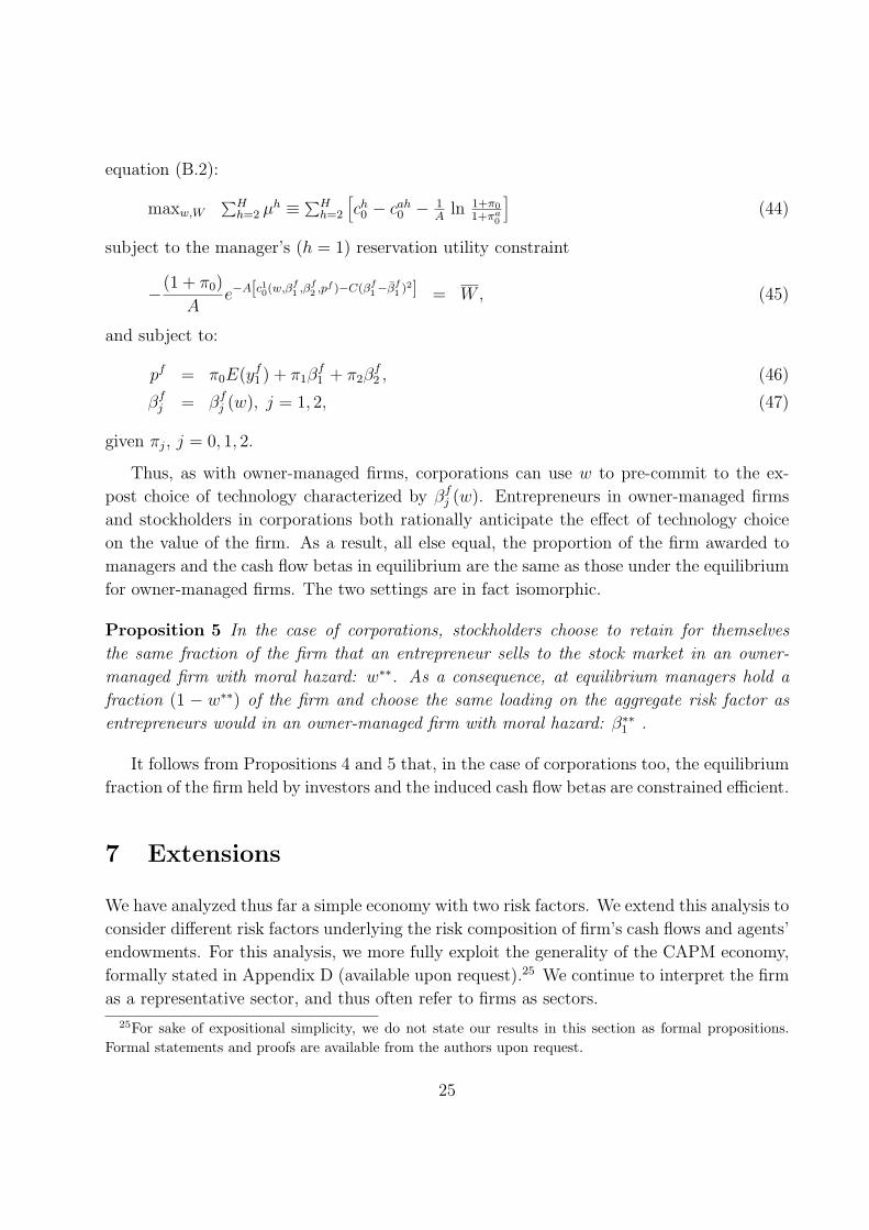
Thus, as with owner-managed firms, corporations can use w to pre-commit to the ex-

post choice of technology characterized by βfj (w). Entrepreneurs in owner-managed firms

and stockholders in corporations both rationally anticipate the effect of technology choice

on the value of the firm. As a result, all else equal, the proportion of the firm awarded to

managers and the cash flow betas in equilibrium are the same as those under the equilibrium

for owner-managed firms. The two settings are in fact isomorphic.

Proposition 5 In the case of corporations, stockholders choose to retain for themselves

the same fraction of the firm that an entrepreneur sells to the stock market in an owner-

managed firm with moral hazard: w∗∗. As a consequence, at equilibrium managers hold a

fraction (1 − w∗∗) of the firm and choose the same loading on the aggregate risk factor as

entrepreneurs would in an owner-managed firm with moral hazard: β∗∗1 .

It follows from Propositions 4 and 5 that, in the case of corporations too, the equilibrium

fraction of the firm held by investors and the induced cash flow betas are constrained efficient.

7 Extensions

We have analyzed thus far a simple economy with two risk factors. We extend this analysis to

consider different risk factors underlying the risk composition of firm’s cash flows and agents’

endowments. For this analysis, we more fully exploit the generality of the CAPM economy,

formally stated in Appendix D (available upon request).25 We continue to interpret the firm

as a representative sector, and thus often refer to firms as sectors.

25For sake of expositional simplicity, we do not state our results in this section as formal propositions.Formal statements and proofs are available from the authors upon request.

25

7.1 Multi-Sector Economy

Consider an economy and a stock market with two sectors, f and g. The economy’s factor

structure is composed of a common risk factor, x1, and two additional risk factors, x2 and

x3, which are orthogonal to the common factor. In this multi-sector economy, the common

factor can be interpreted as a “stock market index,” and the additional risk factors can be

interpreted as the “sector-specific” risks. The cash flows of the two sectors in terms of this

basic factor structure of the economy are as follows:

yf1 − E(yf

1 ) ≡ βf1 x1 + βf

2 x2, (48)

yg1 − E(yg

1) ≡ βg1x1 + βg

3x3. (49)

Entrepreneurs cannot trade the shares of their own firms, but can trade otherwise in the

stock market: entrepreneurs in sector f (respectively in sector g) can trade factors x1 and

x3 (respectively x1 and x2).

At equilibrium, entrepreneurs load their firms’ cash flows on x1, the component of cash

flows that is common with the stock market index and is correlated with the aggregate

endowment risk. Consequently, the cash flows of firms traded in the stock market, and

by implication the stock returns of these firms, are excessively correlated across sectors, in

addition to being correlated with the index returns and the aggregate portfolio.

More formally, entrepreneurs in sector f would want to trade the stock of sector g only as

a way to hedge a part of endowment risk. Entrepreneurs in sector f do not have incentives

to trade factor x3, which is uncorrelated with their wealth. They trade in the stock market

index x1 only.26 The argument is symmetric for entrepreneurs in sector g. Again, in general,

the excessive correlation of stock market returns across sectors is enhanced for firms and

economies that employ high-powered incentive compensation schemes to address alternative

agency problems.

7.2 Purely Idiosyncratic Risk in the Stock Market

Consider a firm in our single-sector economy as in fact a continuum of identical firms of

measure 1, indexed by s ∈ (0, 1), and facing independent and identically distributed (i.i.d.)

26In fact the equilibrium entrepreneurial ownership (1− w∗∗) and the equilibrium loading β∗∗1 are chosenexactly as in Section 3 if the cost function for technology changes is commensurate.

26

shocks.27 We perturb our basic decomposition of stock market returns as follows:

yf,s1 − E(yf

1 ) ≡ βf1 x1 + βf

2 (x2 + xs2) , s ∈ (0, 1). (50)

Factor xs2 represents firm s’s purely idiosyncratic component: It is i.i.d. over s, uncorrelated

with x1 and x2, and it satisfies E(xs2) = 0 and var(xs

2) = σ. An entrepreneur cannot trade

the shares of his own firm and of other firms in his sector, but can trade in the stock market

otherwise. Specifically, entrepreneurs can trade factors x1, but cannot trade (x2 + xs2): The

entrepreneur in firm s must hold the sector-specific component of his firm, x2, as well as the

purely idiosyncratic risk component, xs2.

Entrepreneurs have incentives to over-load their firms’ risk onto the hedgeable component

x1 and away from the unhedgeable component (x2+xs2). The resources entrepreneurs employ

to reduce the loading of the firm on xs2 are wasted from the point of view of the economy: Each

unhedgeable unit of the firm carries a variance of (1+σ) when held by the entrepreneur; the

same unit, when sold to investors, carries an effective variance of 1, as investors can diversify

away xs2 across the continuum of firms. Thus, in equilibrium the fraction of their firms that

entrepreneurs hold decreases in σ, and the induced loading of each firm on the common stock

market component x1 increases in σ. In particular, for any σ > 0, this loading is greater

than β∗∗1 , the equilibrium loading for σ = 0.

8 The Effect of Financial Innovations

We have treated financial markets as exogenous in our analysis. However, incentives to

increase aggregate risk loading of firms depend on the financial markets in the economy;

entrepreneurs and managers will load their firms’ returns on those aggregate risk factors that

they are not restricted from trading in order to hedge their risk exposure. We analyze the

effect of introducing financial innovations that allow greater hedging of such risk exposure.

The impact depends on the specific form of the innovations. More precisely, innovations

that allow the entrepreneurs and managers to hedge their sector-specific risk have a negative

effect on incentives and thus possibly on welfare.28 In contrast, innovations that enable the

27Working with a continuum of firms that face i.i.d. shocks requires abusing the Law of Large Numbers.Working instead with a countable infinity of firms would avoid this abuse with no change to our analysis,but at a notational cost. See, for example, Al-Najjar (1995).

28Even though such financial innovations generally have negative welfare effects for the economy as awhole, financial markets tend to introduce such financial instruments: entrepreneurs and managers will infact demand them. As previously discussed, to manage labor income risk for CEOs and senior executives,investment banks have created a sizable market to manufacture derivative products. Bettis, Bizjak, and

27

entrepreneurs and managers to diversify only the firm-specific or purely idiosyncratic risks

tend to have a positive effect on their incentives and overall welfare.

These points can be easily illustrated. Consider the entrepreneurs of firm f in Section

7.1. What is the effect of a financial innovation that allows these entrepreneurs to hedge x2,

the risk of their sector? This financial innovation allows entrepreneurs to undo the incentives

provided by the ownership of their firm to reduce the aggregate risk of the firm’s cash flows:

Their exposure to any sector-specific risk can be re-balanced after the firm is sold on the

market. Consequently, in equilibrium the fraction of their firms that entrepreneurs hold

coincides with the market share of the firm, (1 − w∗); the loading on the common stock

market component x1 is not reduced at all and coincides with the initial loading βf1 . This

result represents a complete lack of entrepreneurial activity.

In contrast, consider an innovation that allows entrepreneurs to hedge the idiosyncratic

component of the firm’s return, xs2, but not the sector-specific component, x2 (based on the

factor structure of Section 7.2). In this case, entrepreneurs hedge xs2, as do all other agents.

As a consequence, xs2 has no effect on the economy whatsoever, and, in particular, entrepre-

neurs do not shy away from undertaking this risk. Thus, in equilibrium, entrepreneurs hold

a fraction (1− w∗∗) of the firm; and the effect of the innovation is to reduce the loading on

the common stock market component to β∗∗1 . It follows that this innovation in fact has a

positive welfare effect on the economy: It enables greater risk-sharing amongst agents and

reduces wasteful diversification activity.

This analysis of financial innovations that allow entrepreneurs to better hedge their firm’s

idiosyncratic risk could help explain the finding of Campbell, Lettau, Malkiel, and Xu (2001)

that, over the period 1962–1987, the U.S. stock market as a whole did not become more

volatile, even though individual firm volatility increased substantially. The increase in in-

dividual firm volatility could result, at least in part, from such financial innovations having

led managers and entrepreneurs to reduce wasteful activity aimed at reducing firm-specific

risk. Campbell, Lettau, Malkiel, and Xu (2001) also document a decline in the correlation

between individual stock returns. This is consistent with the reduced incentives of man-

agers to substitute firm-specific risks with hedgeable economy-wide risks. Bettis, Bizjak,

and Lemmon (1999) document that the purchases of zero-cost collars and equity swaps by

corporate insiders are followed by an increase in the volatility of their stocks’ returns. While

Bettis, Bizjak, and Lemmon do not isolate the systematic and the idiosyncratic components

of volatility, their evidence is potentially consistent with our argument.

Lemmon (1999) provide direct evidence for managerial demand for such financial innovations. Ofek andYermack (2000) also document the managerial propensity to actively re-balance their portfolios within therestrictions on the sale of their shareholdings.

28

9 Conclusions

In this paper, we examine implications for capital budgeting arising from a manager’s ability

to hedge the aggregate risk of his exposure to firm cash flows. In particular, we focus on

the incentives of managers to substitute the firm-specific risk of cash flows for aggregate

risk, for example, by passing up entrepreneurial activity in favor of more prosaic projects.

We show that such risk-substitution moral hazard increases aggregate risk in stock markets

and reduces the ability of investors to share risks. We characterize the optimal ownership

structure designed to counteract this moral hazard and study its welfare properties.

Our objective has been to identify managerial incentives as an endogenous determinant

of the extent of aggregate or economy-wide risk. Our integrated model could be of more

general use in financial economics. Potential applications include analysis of cross-sectional

and time-series variation in firm-level and market-level volatility, and an in-depth study of

changes in the risk composition of firms following corporate mergers and acquisitions.

References

Acharya, V. and A. Bisin (2000) Optimal Financial-Market Integration and Security Design,

forthcoming, Journal of Business.

Aggarwal, R. and A. Samwick (2003) Why Do Managers Diversify Their Firms? Agency

Reconsidered, Journal of Finance, 58(1), 71–118.

Allen, F. and D. Gale (1988) Optimal Security Design, Review of Financial Studies, 1,

229–263.

Allen, F. and D. Gale (1991) Arbitrage, Short Sales and Financial Innovation, Economet-

rica, 59, 1041–1068.

Al-Najjar, N. I. (1995) Decomposition and Characterization of Risk with a Continuum of

Random Variables, Econometrica, 63, 1195–1224.

Amihud, Y. and B. Lev (1981) Risk Reduction as a Managerial Motive for Conglomerate

Mergers, Bell (RAND) Journal of Economics, 605–617.

Bebchuk, L., J. Fried, and D. Walker (2002) Managerial Power and Rent Extraction in the

Design of Executive Compensation, University of Chicago Law Review, 69, 751–846.

Bettis, J., J. Bizjak, and M. Lemmon (2001) Managerial Ownership, Incentive Contracting,

and the Use of Zero-Cost Collars and Equity Swaps by Corporate Insiders, Journal of

Financial and Quantitative Analysis, 36, 345–370.

29

Bettis, J., Coles, J. and M. Lemmon (2000) Corporate Policies Restricting Trading by

Insiders, Journal of Financial Economics, 57, 191–220.

Bizjak, J., Brickley, J. and J. Coles (1993) Stock-Based Incentive Compensation, Asym-

metric Information and Investment Behavior, Journal of Accounting and Economics,

16, 349–372.

Bisin, A. and P. Gottardi (1999) Competitive Equilibria with Asymmetric Information,

Journal of Economic Theory, 87, 1-48.

Blanchard, O., F. Lopez-de-Silanez, and A. Shleifer (1994) What Do Firms Do with Cash

Windfalls?, Journal of Financial Economics, 36, 337-60.

Campbell, J., Lettau, M., Malkiel, B. and Y. Xu (2001) Have Individual Stocks Become

More Volatile? An Empirical Investigation of Idiosyncratic Risk, Journal of Finance,

56(1), 1–43.

Coles, J. L., Lemmon, M. L., and J. F. Meschke (2003) Structural Models and Endogeneity

in Corporate Finance, Working Paper, College of Business, Arizona State University.

Core, J. E., Guay, W., and D. F. Larcker (2003) Executive Equity Compensation and

Incentives: A Survey, Federal Reserve Board of New York – Economic Policy Review,

forthcoming.

Demsetz, H. and K. Lehn (1985) The Structure of Corporate Ownership: Causes and

Consequences, Journal of Political Economy, 93, 1155–1177.

Denis, D., Denis, D. and A. Sarin (1997) Agency Problems, Equity Ownership, and Cor-

porate Diversification, Journal of Finance, 52(1), 135–160.

Diamond, D. and R. Verrechia (1982) Optimal Managerial Contracts and Equilibrium Se-

curity Prices, Journal of Finance, 37, 275–288.

Easterbrook, F (2002) Derivatives and Corporate Governance, mimeo, University of Chicago

Law Review Symposium.

Fama, E. and M. Miller, (1972) The Theory of Finance, Dryden Press, Hinsdale, IL.

Garvey, G. and T. Milbourn (2002) Incentive Compensation When Executives Can Hedge

the Market: Evidence of RPE in the Cross-Section, Journal of Finance, forthcoming.

Hermalin, B. and M. Weisbach (1991) The Effects of Board Compensation and Direct

Incentives of Firm Performance, Financial Management, 20, 101-12.

30

Himmelberg, C., Hubbard, G. R. and I. Love (2002) Investor Protection, Ownership, and

the Cost of Capital, Working Paper, Columbia University.

Holmstrom, B. and P. Milgrom (1987) Aggregation and Linearity in the Provision of In-

tertemporal Incentives, Econometrica, 55, 303–328.

Jensen, M. (1986) The Agency Cost of Free Cash Flow: Corporate Finance and Takeovers,

American Economic Review, 76(2), 323-30.

Jensen, M. and W. Meckling (1976) Theory of the Firm: Managerial Behavior, Agency

Costs and Ownership Structure, Journal of Financial Economics, 3, 305-360.

Jin, L. (2002) CEO Compensation, Diversification and Incentives: Theory and Empirical

Results, Journal of Financial Economics, 66(1), 29–63.

Laffont, J. and D. Martimort (2002) The Theory of Incentives: The Principal-Agent Model,

Princeton University Press.

Lambert, R. (1986) Executive Effort and Selection of Risky Projects, Rand Journal of

Economics, 17(1), 77–88.

Lamont, O. and C. Polk (2001) The Diversification Discount: Cash Flows versus Returns,

Journal of Finance, LVI(5), 1693-722.

Lang, L., R. Stulz, and R. Walking (1991) A Test of the Free Cash Flow Hypothesis, Journal

of Financial Economics, 24, 181-92.

Magill, M. and M. Quinzii (2002) Capital Market Equilibrium with Moral Hazard, Journal

of Mathematical Economics,38, 149-190.

Mann, S. and N. Sicherman (1991) The Agency Costs of Free Cash Flow: Acquisition

Activity and Equity Issues, Journal of Business, 64, 213-27.

May, P. (1995) Do Managerial Motives Influence Firm Risk Reduction Strategies? Journal

of Finance, 50(4), 1291–1308.

McConnell, J. and H. Servaes (1990) Additional Evidence on Equity Ownership and Cor-

porate Value, Journal of Financial Economics, 27, 595–612.

McConnell, J. and H. Servaes (1995) Equity Ownership and the Two Faces of Debt, Journal

of Financial Economics, 39, 131-57.

McConnell, J., H. Servaes, and K.V. Lins (2004) Changes in Equity Ownership and Changes

in the Market Value of the Firm, Working Paper, Krannert School of Management,

Purdue University.

31

Morck, R., A. Shleifer and R. Vishny (1988) Management Ownership and Market Valuation:

An Empirical Analysis, Journal of Financial Economics , 293–315.

Ofek, E. and D. Yermack (2000) Taking Stock: Equity-Based Compensation and the Evo-

lution of Managerial Ownership, Journal of Finance, 55(3), 1367–1384.

Ou-Yang, H. (2002) An Equilibrium Model of Asset Pricing and Moral Hazard, Working

Paper, Fuqua School of Business, Duke University.

Prescott, E. and R. Townsend (1984) Optima and Competitive Equilibria with Adverse

Selection and Moral Hazard, Econometrica, 52, 21-45.

Ramakrishnan, R. and A. Thakor (1984) The Valuation of Assets under Moral Hazard,

Journal of Finance, 39(1), 229–238.

Schizer, D. (2000) Executives and Hedging: The Fragile Foundation of Incentive Compati-

bility, Columbia Law Review, 100, 440–504.

Willen, P. (1997) Some Notes on CAPM, mimeo, Princeton University.

32

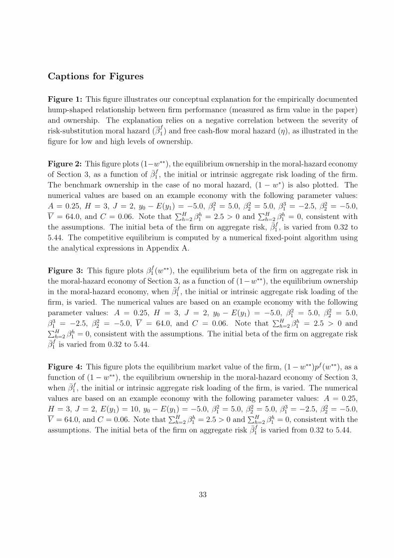
Captions for Figures

Figure 1: This figure illustrates our conceptual explanation for the empirically documented

hump-shaped relationship between firm performance (measured as firm value in the paper)

and ownership. The explanation relies on a negative correlation between the severity of

risk-substitution moral hazard (βf

1) and free cash-flow moral hazard (η), as illustrated in the

figure for low and high levels of ownership.

Figure 2: This figure plots (1−w∗∗), the equilibrium ownership in the moral-hazard economy

of Section 3, as a function of βf1 , the initial or intrinsic aggregate risk loading of the firm.

The benchmark ownership in the case of no moral hazard, (1 − w∗) is also plotted. The

numerical values are based on an example economy with the following parameter values:

A = 0.25, H = 3, J = 2, y0 − E(y1) = −5.0, β21 = 5.0, β2

2 = 5.0, β31 = −2.5, β2

2 = −5.0,

V = 64.0, and C = 0.06. Note that∑H

h=2 βh1 = 2.5 > 0 and

∑Hh=2 βh

1 = 0, consistent with

the assumptions. The initial beta of the firm on aggregate risk, βf1 , is varied from 0.32 to

5.44. The competitive equilibrium is computed by a numerical fixed-point algorithm using

the analytical expressions in Appendix A.

Figure 3: This figure plots βf1 (w∗∗), the equilibrium beta of the firm on aggregate risk in

the moral-hazard economy of Section 3, as a function of (1−w∗∗), the equilibrium ownership

in the moral-hazard economy, when βf1 , the initial or intrinsic aggregate risk loading of the

firm, is varied. The numerical values are based on an example economy with the following

parameter values: A = 0.25, H = 3, J = 2, y0 − E(y1) = −5.0, β21 = 5.0, β2

2 = 5.0,

β31 = −2.5, β2

2 = −5.0, V = 64.0, and C = 0.06. Note that∑H

h=2 βh1 = 2.5 > 0 and∑H

h=2 βh1 = 0, consistent with the assumptions. The initial beta of the firm on aggregate risk

βf1 is varied from 0.32 to 5.44.

Figure 4: This figure plots the equilibrium market value of the firm, (1−w∗∗)pf (w∗∗), as a

function of (1− w∗∗), the equilibrium ownership in the moral-hazard economy of Section 3,

when βf1 , the initial or intrinsic aggregate risk loading of the firm, is varied. The numerical

values are based on an example economy with the following parameter values: A = 0.25,

H = 3, J = 2, E(y1) = 10, y0 − E(y1) = −5.0, β21 = 5.0, β2

2 = 5.0, β31 = −2.5, β2

2 = −5.0,

V = 64.0, and C = 0.06. Note that∑H

h=2 βh1 = 2.5 > 0 and

∑Hh=2 βh

1 = 0, consistent with the

assumptions. The initial beta of the firm on aggregate risk βf1 is varied from 0.32 to 5.44.

33

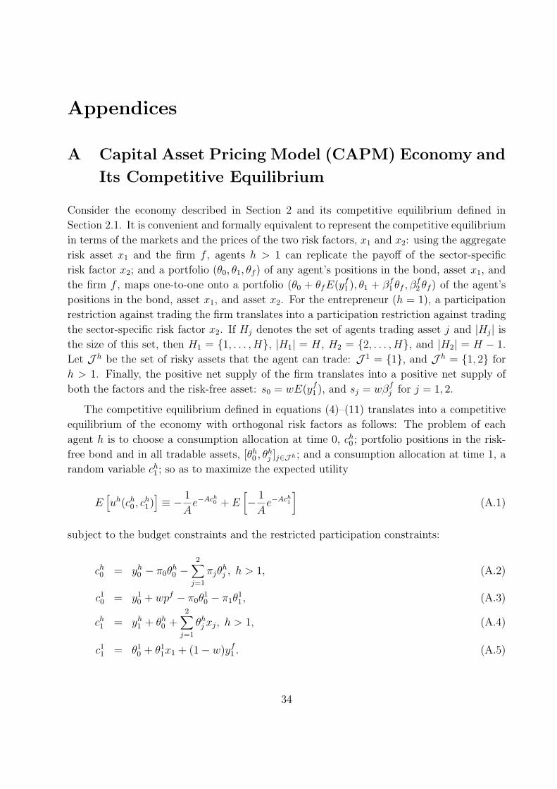
Appendices

A Capital Asset Pricing Model (CAPM) Economy and

Its Competitive Equilibrium

Consider the economy described in Section 2 and its competitive equilibrium defined in

Section 2.1. It is convenient and formally equivalent to represent the competitive equilibrium

in terms of the markets and the prices of the two risk factors, x1 and x2: using the aggregate

risk asset x1 and the firm f , agents h > 1 can replicate the payoff of the sector-specific

risk factor x2; and a portfolio (θ0, θ1, θf ) of any agent’s positions in the bond, asset x1, and

the firm f , maps one-to-one onto a portfolio (θ0 + θfE(yf1 ), θ1 + βf

1 θf , βf2 θf ) of the agent’s

positions in the bond, asset x1, and asset x2. For the entrepreneur (h = 1), a participation

restriction against trading the firm translates into a participation restriction against trading

the sector-specific risk factor x2. If Hj denotes the set of agents trading asset j and |Hj| is

the size of this set, then H1 = 1, . . . , H, |H1| = H, H2 = 2, . . . , H, and |H2| = H − 1.

Let J h be the set of risky assets that the agent can trade: J 1 = 1, and J h = 1, 2 for

h > 1. Finally, the positive net supply of the firm translates into a positive net supply of

both the factors and the risk-free asset: s0 = wE(yf1 ), and sj = wβf

j for j = 1, 2.

The competitive equilibrium defined in equations (4)–(11) translates into a competitive

equilibrium of the economy with orthogonal risk factors as follows: The problem of each

agent h is to choose a consumption allocation at time 0, ch0 ; portfolio positions in the risk-

free bond and in all tradable assets, [θh0 , θh

j ]j∈J h ; and a consumption allocation at time 1, a

random variable ch1 ; so as to maximize the expected utility

E[uh(ch

0 , ch1)]≡ − 1

Ae−Ach

0 + E[− 1

Ae−Ach

1

](A.1)

subject to the budget constraints and the restricted participation constraints:

ch0 = yh

0 − π0θh0 −

2∑j=1

πjθhj , h > 1, (A.2)

c10 = y1

0 + wpf − π0θ10 − π1θ

11, (A.3)

ch1 = yh

1 + θh0 +

2∑j=1

θhj xj, h > 1, (A.4)

c11 = θ1

0 + θ11x1 + (1− w)yf

1 . (A.5)

34

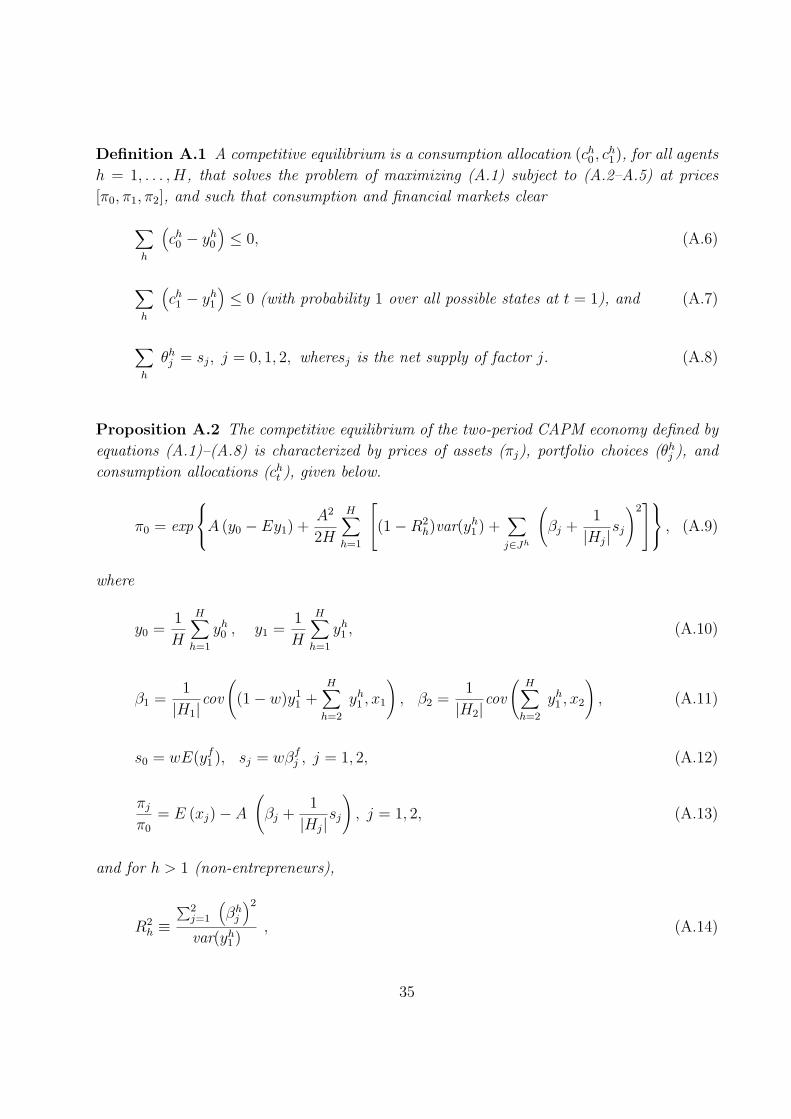
Definition A.1 A competitive equilibrium is a consumption allocation (ch0 , c

h1), for all agents

h = 1, . . . , H, that solves the problem of maximizing (A.1) subject to (A.2–A.5) at prices

[π0, π1, π2], and such that consumption and financial markets clear

∑h

(ch0 − yh

0

)≤ 0, (A.6)

∑h

(ch1 − yh

1

)≤ 0 (with probability 1 over all possible states at t = 1), and (A.7)

∑h

θhj = sj, j = 0, 1, 2, wheresj is the net supply of factor j. (A.8)

Proposition A.2 The competitive equilibrium of the two-period CAPM economy defined by

equations (A.1)–(A.8) is characterized by prices of assets (πj), portfolio choices (θhj ), and

consumption allocations (cht ), given below.

π0 = exp

A (y0 − Ey1) +A2

2H

H∑h=1

(1−R2h)var(y

h1 ) +

∑j∈Jh

(βj +

1

|Hj|sj

)2 , (A.9)

where

y0 =1

H

H∑h=1

yh0 , y1 =

1

H

H∑h=1

yh1 , (A.10)

β1 =1

|H1|cov

((1− w)y1

1 +H∑

h=2

yh1 , x1

), β2 =

1

|H2|cov

(H∑

h=2

yh1 , x2

), (A.11)

s0 = wE(yf1 ), sj = wβf

j , j = 1, 2, (A.12)

πj

π0

= E (xj)− A

(βj +

1

|Hj|sj

), j = 1, 2, (A.13)

and for h > 1 (non-entrepreneurs),

R2h ≡

∑2j=1

(βh

j

)2

var(yh1 )

, (A.14)

35

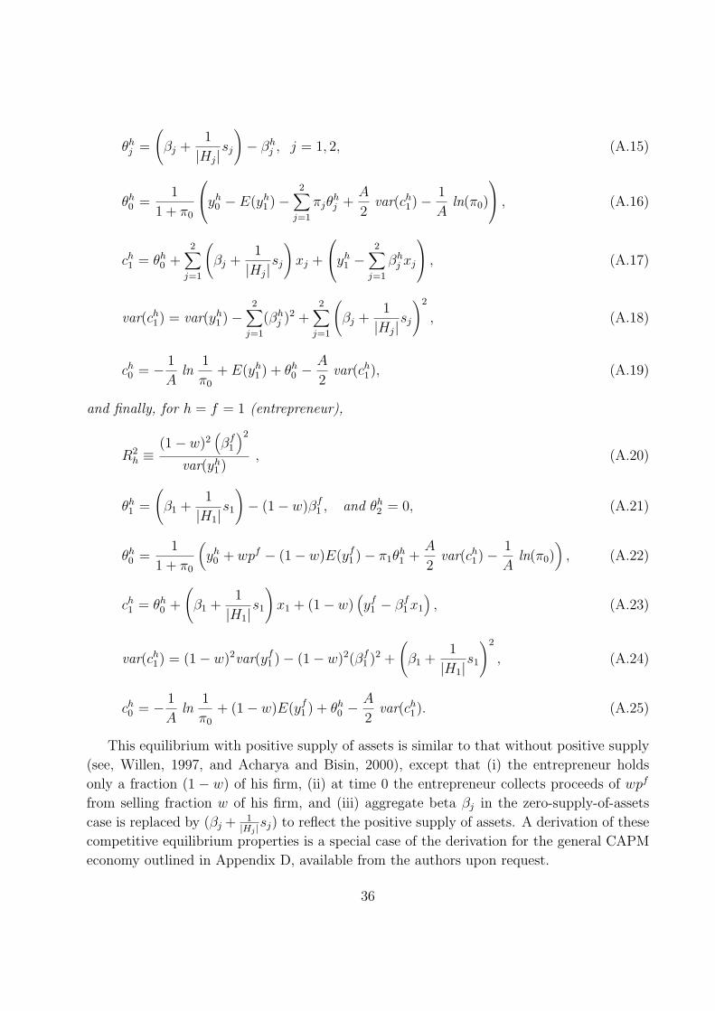
θhj =

(βj +

1

|Hj|sj

)− βh

j , j = 1, 2, (A.15)

θh0 =

1

1 + π0

yh0 − E(yh

1 )−2∑

j=1

πjθhj +

A

2var(ch

1)−1

Aln(π0)

, (A.16)

ch1 = θh

0 +2∑

j=1

(βj +

1

|Hj|sj

)xj +

yh1 −

2∑j=1

βhj xj

, (A.17)

var(ch1) = var(yh

1 )−2∑

j=1

(βhj )2 +

2∑j=1

(βj +

1

|Hj|sj

)2

, (A.18)

ch0 = − 1

Aln

1

π0

+ E(yh1 ) + θh

0 −A

2var(ch

1), (A.19)

and finally, for h = f = 1 (entrepreneur),

R2h ≡

(1− w)2(βf

1

)2

var(yh1 )

, (A.20)

θh1 =

(β1 +

1

|H1|s1

)− (1− w)βf

1 , and θh2 = 0, (A.21)

θh0 =

1

1 + π0

(yh

0 + wpf − (1− w)E(yf1 )− π1θ

h1 +

A

2var(ch

1)−1

Aln(π0)

), (A.22)

ch1 = θh

0 +

(β1 +

1

|H1|s1

)x1 + (1− w)

(yf

1 − βf1 x1

), (A.23)

var(ch1) = (1− w)2var(yf

1 )− (1− w)2(βf1 )2 +

(β1 +

1

|H1|s1

)2

, (A.24)

ch0 = − 1

Aln

1

π0

+ (1− w)E(yf1 ) + θh

0 −A

2var(ch

1). (A.25)

This equilibrium with positive supply of assets is similar to that without positive supply

(see, Willen, 1997, and Acharya and Bisin, 2000), except that (i) the entrepreneur holds

only a fraction (1 − w) of his firm, (ii) at time 0 the entrepreneur collects proceeds of wpf

from selling fraction w of his firm, and (iii) aggregate beta βj in the zero-supply-of-assets

case is replaced by (βj + 1|Hj |sj) to reflect the positive supply of assets. A derivation of these

competitive equilibrium properties is a special case of the derivation for the general CAPM

economy outlined in Appendix D, available from the authors upon request.

36

B Welfare Properties

We characterize the welfare measure used in the paper (individual h’s compensating transfer,

µh, and the aggregate compensating transfer, µ) in terms of the equilibrium price of the bond,

π0, and the exogenously given price of the bond at autarky, πa0 .

Proposition B.1 The individual welfare of agent h is measured by

µ1 = c10 − ca1

0 − 1

Aln

1 + π0

1 + πa0

− C(βf1 − βf

1 )2, and (B.1)

µh = ch0 − cah

0 − 1

Aln

1 + π0

1 + πa0

, for h = 2, . . . , H. (B.2)

The aggregate welfare of the economy is measured by

µ = −H

Aln

1 + π0

1 + πa0

− C(βf1 − βf

1 )2. (B.3)

Proof: Consider the definitions of individual welfare in equations (35) and (36). Since

U1(c10 − C(βf

1 − βf1 )2, c1

1) ≡ −(1 + π0)

Ae−A[c10−C(βf

1−βf1 )2], (B.4)

Uh(ch0 , c

h1) ≡ (1 + π0)

Ae−Ach

0 , for h = 2, . . . , H, and, (B.5)

Uah(cah0 + µh, cah

1 ) ≡ −(1 + πa0)

Ae−Acah

0 , ∀h, (B.6)

we obtain that µ1, the individual welfare of entrepreneur, satisfies

(1 + π0)

Ae−A[c10−C(βf

1−βf1 )2] =

(1 + πa0)

Ae−A(ca1

0 +µ1) . (B.7)

Simplifying this, we obtain the expression for µ1 in equation (B.1). The result for µh, h =

2, . . . , H, follows similarly. Finally, since µ =∑H

h=1 µh, and∑H

h=1 ch0 =

∑Hh=1 cah

0 =∑H

h=1 yh0

by the market-clearing conditions under both economies, we obtain the expression for µ in

equation (B.3). ♦

C Proofs of Propositions

Proof of Proposition 1. Under the benchmark case in equation (21), the entrepreneur

simultaneously chooses the ownership structure, w, and the cash flow betas, βf1 and βf

2 . We

37

first consider the choice of βf1 for a given w, and next the choice of optimal w, taking into

account the choice of βf1 ; βf

2 is determined by the constraint (23).

The entrepreneur is a price-taker and trades only in asset 0 and asset 1, but rationally

anticipates the effect of cash flow betas on the price of the firm pf (equation 22). Using the

competitive equilibrium outcomes (A.21)–(A.25) from Appendix A, we obtain

∂

∂βf1

[c10(w, βf

1 , βf2 , pf = π0E(yf

1 ) + π1βf1 + π2β

f2 )− C(βf

1 − βf1 )2]

(C.1)

=∂

∂βf1

[θ10 −

A

2var(c1

1)]− 2C(βf

1 − βf1 ) (C.2)

=∂

∂βf1

[1

1 + π0

(wπ1β

f1 + wπ2β

f2 + (1− w)π1β

f1 −

Aπ0

2var(c1

1))]− 2C(βf

1 − βf1 )

=π1

1 + π0

− π2w

1 + π0

βf1

βf2

+A π0

1 + π0

(1− w)2βf1 − 2C(βf

1 − βf1 ) (C.3)

=A π0

1 + π0

[((1− w)2 +

w2

H − 1− 1

H

)βf

1 −1

H

H∑h=2

βh1

]− 2C(βf

1 − βf1 ), (C.4)

where, to obtain equation (C.3), we substitute constraints (22) and (23) and the restricted

participation constraints θ12 ≡ 0, |H1| = H, and |H2| = H − 1. Finally, to obtain equation

(C.4) from equation (C.3), we substitute equilibrium prices and aggregate supplies using

equations (A.11)–(A.13) and the maintained assumption (equation 17) that β2 = 0. The

optimal βf1 for a given w sets the partial derivative in equation (C.4) to zero.

Consider next the choice of w given the choice of βf1 .

d[c10 − C(βf

1 − βf1 )2]

dw=

∂[c10 − C(βf

1 − βf1 )2]

∂βf1

dβf1

dw+

∂[c10 − C(βf

1 − βf1 )2]

∂w(C.5)

=∂[c1

0 − C(βf1 − βf

1 )2]

∂wby the envelope theorem. (C.6)

Since the entrepreneur is a price-taker, using equations (A.21)–(A.25) we obtain

∂[c10 − C(βf

1 − βf1 )2]

∂w=

∂c10

∂w=

∂

∂w

[(1− w)E(yf

1 ) + θ10 −

A

2var(c1

1)], where (C.7)

θ10 −

A

2var(c1

1) =1

1 + π0

y10 − (1− w)E(yf

1 ) + π0wE(yf1 ) +

2∑j=1

πjwβfj − π1θ

11

− Aπ0

2(1 + π0)var(c1

1)−1

A(1 + π0)ln(π0). (C.8)

38

Simplifying using constraints (22) and (23), the maintained assumptions, and the expressions

for equilibrium prices and aggregate supplies in equations (A.11)–(A.13), we obtain

∂[c10 − C(βf

1 − βf1 )2]

∂w= −E(yf

1 ) +1

1 + π0

[(1 + π0)E(yf

1 ) + π2βf2 + A π0(1− w)(βf

2 )2]

=1

1 + π0

[π2β

f2 + Aπ0(1− w)(βf

2 )2]

(C.9)

=A π0

1 + π0

(βf2 )2

(1− w − w

H − 1

). (C.10)

This first-order derivative is set to zero at w = w∗ ≡ (1− 1H

). Furthermore,

d2[c10 − C(βf

1 − βf1 )2]

dw2=

d

dw

(∂[c1

0 − C(βf1 − βf

1 )2]

∂w

)=

∂2[c10 − C(βf

1 − βf1 )2]

∂w2(C.11)

= − HAπ0

(H − 1)(1 + π0)(βf

2 )2 < 0, since (C.12)

∂2[c10 − C(βf

1 − βf1 )2]

∂βf1 ∂w

=∂

∂βf1

[A π0

1 + π0

(βf2 )2

(1− w − w

H − 1

)](C.13)

= − 2 A π0

1 + π0

βf1

(1− w − w

H − 1

)= 0 at w = w∗. (C.14)

The equity ownership retained by the entrepreneur is thus given by (1 − w∗) = 1H

.

Substituting w = w∗ in equation (C.4) and setting it to zero, we find that the aggregate-risk

beta chosen by the entrepreneur is β∗1 = βf1 − Aπ0

2CH(1+π0)

∑Hh=2 βh

1 < βf1 . Note that at w = w∗,

∂2

∂βf2

1

[c10 − C(βf

1 − βf1 )2] = −2ACπ0

1+π0< 0, satisfying the optimality of β∗1 . ♦

Proof of Propositions 2.

Sequence of Steps: First, we characterize the technology choice β∗∗1 and the ownership

structure choice w∗∗ for the case of owner-managed firm with moral hazard (Proposition 2).

Next, we prove that the equilibrium aggregate risk loading in the moral-hazard case exceeds

the benchmark aggregate risk loading, i.e., β∗1 < β∗∗1 .

Step 1: First consider the entrepreneur’s technology choice for owner-managed firms with

moral hazard as specified in equation (24). The analysis differs from the proof of Proposition

1 (the case of no moral hazard) as follows: From the entrepreneur’s standpoint, the firm’s

proceeds cannot be affected by a choice of betas, because the betas are not observed by

investors. Formally, this implies that the constraint pf = π0E(yf1 ) + π1β

f1 + π2β

f2 (equation

22) does not affect the capital budgeting problem in the case of moral hazard. Define

c10 ≡ c1

0(w, βf1 , βf

2 , pf ), where pf is treated as a lump sum constant in order to distinguish it

from c10 ≡ c1

0(w, βf1 , βf

2 , pf = π0E(yf1 ) + π1β

f1 + π2β

f2 ).

39

Using the competitive equilibrium outcomes (A.21)–(A.25), we obtain

∂

∂βf1

[c10(w, βf

1 , βf2 , pf )− C(βf

1 − βf1 )2]

(C.15)

=∂

∂βf1

[θ10 −

A

2var(c1

1)]− 2C(βf

1 − βf1 ) (C.16)

=∂

∂βf1

[1

1 + π0

((1− w)π1β

f1 −

Aπ0

2var(c1

1))]− 2C(βf

1 − βf1 ) (C.17)

=π1(1− w)

1 + π0

+A π0

1 + π0

(1− w)2βf1 − 2C(βf

1 − βf1 ) (C.18)

=A π0

1 + π0

(1− w)

[(1− w − 1

H

)βf

1 −1

H

H∑h=2

βh1

]− 2C(βf

1 − βf1 ), (C.19)

where, to obtain equation (C.18), we substitute only the constraint (25) and the restricted

participation constraints θ12 ≡ 0, |H1| = H, and |H2| = H − 1; finally, to obtain equation

(C.19) from equation (C.18), we substitute equilibrium prices and aggregate supplies using

equations (A.11)–(A.13) and the maintained assumption that β2 = 0.

Let βf1 (w) be the choice of βf

1 that sets the partial derivative in equation (C.19) to zero.

The solution to the capital budgeting problem in (24) is thus given by

βf1 (w) = K1(w)βf

1 −K2(w)H∑

h=2

βh1 , where (C.20)

K1(w) =

[1− Aπ0(1− w)

2C(1 + π0)

(1− w − 1

H

)]−1

, and (C.21)

K2(w) =Aπ0(1− w)

2CH(1 + π0)K1(w). (C.22)

Next, consider the choice of w by the entrepreneur of the owner-managed firm, as specified

in equation (26). While choosing w, the rational expectation constraints apply both for the

firm value (equation 27) and for the effect of w on βf1 (equation 28). Thus, we obtain

d[c10 − C(βf

1 − βf1 )2]

dw=

∂[c10 − C(βf

1 − βf1 )2]

∂βf1

dβf1 (w)

dw+

∂[c10 − C(βf

1 − βf1 )2]

∂w(C.23)

where c10 ≡ c1

0(w, βf1 (w), βf

2 (w), pf = π0E(yf1 ) + π1β

f1 + π2β

f2 ) as distinct from c1

0 ≡ c10(w, βf

1 , βf2 , pf ).

We examine successively each of the three terms in the above equation.

(I) First, note that

∂[c10 − C(βf

1 − βf1 )2]

∂w=

A π0

1 + π0

(βf2 )2

(1− w − w

H − 1

)= 0 at w = w∗, (C.24)

40

as in the case of no moral hazard (see equation C.10 in the proof of Proposition 1, above).

(II) Second, we examine∂[c10−C(βf

1−βf1 )2]

∂βf1

. Note that, unlike the case of no moral hazard,

∂[c10−C(βf1−βf

1 )2]

∂βf1

6= 0 (in general), since βf1 (w) is chosen treating pf as a lump sum constant.

That is, βf1 (w) is chosen such that

∂[c10−C(βf1−βf

1 )2]

∂βf1

= 0, which is not generally the same as

∂[c10−C(βf1−βf

1 )2]

∂βf1

= 0. Thus, when βf1 = βf

1 (w),

∂[c10 − C(βf

1 − βf1 )2]

∂βf1

=∂[c1

0 − C(βf1 − βf

1 )2]

∂βf1

− ∂(c10 − c1

0)

∂βf1

= − ∂(c10 − c1

0)

∂βf1

, (C.25)

where∂(c1

0 − c10)

∂βf1

=∂

∂βf1

[1

1 + π0

(wpf − π0wE(yf

1 )− π1wβf1 − π2wβf

2

)](C.26)

=1

1 + π0

[−π1w − π2w

(−βf

1

βf2

)](C.27)

=A π0 w

1 + π0

[1

H

(H∑

h=2

βh1 + βf

1

)− w

H − 1βf

1

](C.28)

=A π0 w

H(1 + π0)

[H∑

h=2

βh1 +

(1− w

w∗

)βf

1

], (C.29)

where we have employed the expressions for equilibrium prices and aggregate supplies in

equations (A.11)–(A.13). It follows that at w = w∗,∂[c10−C(βf

1−βf1 )2]

∂βf1

< 0, since∑H

h=2 βh1 > 0.

(III) Finally, we examinedβf

1 (w)

dw. Since

∂[c10−C(βf1−βf

1 )2]

∂βf1

= 0 and∂2[c10−C(βf

1−βf1 )2]

∂βf2

1

< 0 at

βf1 = βf

1 (w) by the optimality of βf1 (w) under moral hazard, it follows that

∂2[c10 − C(βf

1 − βf1 )2]

∂βf1

2

dβf1 (w)

dw+

∂2[c10 − C(βf

1 − βf1 )2]

∂w∂βf1

= 0 (C.30)

⇒ sign

(dβf

1 (w)

dw

)= sign

(∂2[c1

0 − C(βf1 − βf

1 )2]

∂w∂βf1

). (C.31)

From equation (C.19), we obtain

∂2[c10 − C(βf

1 − βf1 )2]

∂w∂βf1

=A π0

1 + π0

[−2(1− w)βf

1 +1

H

(H∑

h=2

βh1 + βf

1

)], (C.32)

where βf1 = βf

1 (w). It follows that at w = w∗ ≡ (1− 1/H),

∂2[c10 − C(βf

1 − βf1 )2]

∂w∂βf1

=A π0

H(1 + π0)

[H∑

h=2

βh1 − βf

1 (w)

]. (C.33)

41

Thus,dβf

1 (w)

dw< 0 at w = w∗ if and only if βf

1 (w∗) >∑H

h=2 βh1 . Substituting w = (1− 1/H) in

equation (C.19) and equating it to zero yields

βf1 (w∗) = βf

1 −Aπ0

2CH2(1 + π0)

H∑h=2

βh1 < βf

1 . (C.34)

It follows from (I), (II), and (III) above that at w = w∗,d[c10−C(βf

1−βf1 )2]

dw> 0 iff βf

1 >

K(π0)∑H

h=2 βh1 , where K(π0) = Aπ0/(2CH2(1+π0))+1. If the cost parameter C is sufficiently

high, then the function [c10−C(βf

1 − βf1 )2] is globally concave.29 Then, the optimal ownership

structure under moral hazard is w∗∗, where w∗∗ > w∗ iff βf1 > K(π0)

∑Hh=2 βh

1 .

Furthermore, since βf1 (w∗) < βf

1 , and in both cases above w∗∗ is chosen to reduce the

aggregate risk loading from its value at w∗, it follows that β∗∗1 = βf1 (w∗∗) < βf

1 (w∗) < βf1 .

Since π0 ∈ [0, 1], K(π0) ∈ [1, K], where K ≡ 1 + A/(4CH2).

Step 2: Next, we prove that the choice of the risk loading, β∗∗1 , is greater than the benchmark

case (first-best), β∗1 . Since w∗∗ is constrained efficient (as proved below in the proof of

Proposition 4), it follows that at w = w∗∗,

dµ

dw=

∂µ

∂βf1

dβf1 (w)

dw+

∂µ

∂w= 0 ⇒ ∂µ

∂βf1

= −

(∂µ∂w

)(

dβf1

dw

) . (C.36)

Now, consider the case where βf1 (w∗) >

∑Hh=2 βh

1 . Then, for the moral-hazard economy,dβf

1 (w)

dw< 0 at w = w∗∗ > w∗. By the first-best efficiency of w∗, we have ∂µ

∂w= 0 and ∂2µ

∂w2 < 0

at w = w∗. This, in turn, implies that ∂µ∂w

< 0 at w = w∗∗. From equation (C.36), we

29Define function g(w, βf1 (w)) ≡ c1

0(w, βf1 , βf

2 , pf = π0E(yf1 ) + π1β

f1 + π2β

f2 ) − C(βf

1 − βf1 )2, where βf

1 =

βf1 (w) and (βf

1 )2 + (βf2 )2 = V . Then,

d2g

dw2=

∂2g

∂w2+ 2

∂2g

∂βf1 ∂w

dβf1 (w)dw

+∂2g

∂βf2

1

(dβf

1 (w)dw

)2

+d2βf

1 (w)dw2

∂g

∂βf1

. (C.35)

Note the following: (i) From equation (C.12), ∂2g∂w2 < 0,∀w; this is the global concavity of the entrepreneur’s

objective as a function of w under the benchmark case. (ii) ∂2g

∂βf21

= ∂2c10

∂βf21

− C < 0 for C sufficiently large.

(iii) Using equation (C.20), it can be shown that dβf1 (w)

dw → 0 as C →∞. (iv) Similarly, it can be shown thatd2βf

1 (w)

dw2 → 0 as C → ∞. (v) From equation (C.13), ∂2g

∂βf1 ∂w

is independent of C. Finally, (vi) from equation

(C.4), ∂g

∂βf1

is bounded. It follows that for C sufficiently large, d2gdw2 < 0,∀w, i.e., if the moral-hazard problem

is not “too severe,” then as a function of w the objective of the entrepreneur under the moral-hazard case isa “perturbation” around the globally concave objective under no moral hazard.

42

conclude that ∂µ

∂βf1

< 0 at w = w∗∗. That is, the choice of βf1 under moral hazard, β∗∗1 ,

exceeds the first-best (for which ∂µ

∂βf1

= 0). The proof for the case where βf1 (w∗) <

∑Hh=2 βh

1

follows analogously. ♦

Proof of Proposition 3. In the first-best specified in equation (38), the equity ownership

structure w and cash flow beta βf1 are chosen by the planner to maximize the compensating

aggregate transfer, µ, given by equation (B.3). Consider first the choice of βf1 by the planner

for a given w. From equation (A.9) for π0 at the competitive equilibrium, we obtain

∂µ

∂βf1

= − H

A(1 + π0)

∂π0

∂βf1

− 2C(βf1 − βf

1 ), where (C.37)

∂π0

∂βf1

=π0A

2

2H

∂

∂βf1

(1− w)2var(yf1 )− (1− w)2(βf

1 )2 +H∑

h=1

∑j∈J h

(βj +

1

|Hj|sj

)2

=π0A

2

2H

∂

∂βf1

−(1− w)2(βf1 )2 +

1

H

(H∑

h=2

βh1 + βf

1

)2

+w2

H − 1(βf

2 )2

(C.38)

=π0A

2

H

[−(1− w)2βf

1 +1

H

(H∑

h=2

βh1 + βf

1

)− w2

H − 1βf

1

], (C.39)

where we have employed constraint (39), conditions (A.11) and (A.12), and β2 = 0. Thus,

∂µ

∂βf1

=A π0

1 + π0

[((1− w)2 +

w2

H − 1− 1

H

)βf

1 −1

H

H∑h=2

βh1

]− 2C(βf

1 − βf1 ), (C.40)

which is identical to the first-order condition for the choice of βf1 by the entrepreneur in the

benchmark case (equation C.4). Thus, for a given w, the first-best choice of βf1 is the same

as that of the entrepreneur in the absence of moral hazard.

Next, consider the planner’s choice of w. By the envelope theorem, we obtain

dµ

dw=

∂µ

∂w= − H

A(1 + π0)

∂π0

∂w, where (C.41)

∂π0

∂w= π0

∂

∂w

A2

2H

(1− w)2var(yf1 )− (1− w)2(βf

1 )2 +H∑

h=1

∑j∈J h

(βj +

1

|Hj|sj

)2

=π0A

2

2H

∂

∂w

(1− w)2(βf2 )2 +

1

H

(H∑

h=2

βh1 + βf

1

)2

+w2

H − 1(βf

2 )2

(C.42)

=π0A

2

2H

[−2(1− w)(βf

2 )2 +2w

H − 1(βf

2 )2]

(C.43)

=π0A

2

H(βf

2 )2(1− w − w

H − 1

). (C.44)

43

The above equations can be simplified to yield

dµ

dw=

A π0

1 + π0

(βf2 )2

(1− w − w

H − 1

), (C.45)

which is identical to the first-order condition for choice of w by the entrepreneur in the bench-

mark case (equation C.10). It follows that in the absence of moral hazard, the entrepreneur’s

choices of w∗ and β∗1 are first-best efficient. ♦

Proof of Proposition 4. The constrained-efficient choice of w is specified in equation (40).

From the proof of the first-best efficiency of the

benchmark case (Proposition 3), we know that ∀w:

∂µ

∂βf1

=∂[c1

0 − C(βf1 − βf

1 )2]

∂βf1

, and∂µ

∂w=

∂[c10 − C(βf

1 − βf1 )2]

∂w. (C.46)

It follows that ∀w:

dµ

dw=

∂µ

∂βf1

dβf1 (w)

dw+

∂µ

∂w=

d[c10 − C(βf

1 − βf1 )2]

dw, (C.47)

where the planner is constrained to choose the samedβf

1 (w)

dwas the entrepreneur. Thus, dµ

dwis

point-wise identical to dµ1

dw(given by equation C.23). In turn, the constrained-efficient choice

of w, which sets dµdw

to zero, is identical to the choice of w for the owner–managed firm with

moral hazard, which sets dµ1

dwto zero. The constrained efficiency of w∗∗ in the owner-managed

firm with moral hazard follows. ♦

Proof of Proposition 5. In the case of corporations, the manager is first awarded a

fraction (1 − w) of the firm as a stock reward, and then the manager chooses βf1 and βf

2 .

Investors retain the remaining fraction w. The initial time-1 endowments for all agents

are thus identical to their endowments in the case of owner-managed firms for the same

fraction w of the firm sold on the stock market. The only change arises at time 0 due to

the time-0 compensation W awarded to the manager to ensure that in equilibrium he earns

the reservation utility of W (see footnote 24). Since these transfers are treated as lump

sum constants while undertaking the choice of technology, the managerial choice βf1 (w) is

identical to that of the owner–manager with moral hazard.

The welfare of investors is equivalent to µ − µ1, where µ equals∑H

h=1 µh, the aggregate

compensating welfare, and µ1 is the individual compensating welfare of the manager. In

equilibrium, µ1 is such that Ua1(ca10 + µ1, ca1) ≡ W , the manager’s reservation utility (see

equation 45 and 36). That is, µ1 is a constant, which implies that the optimal compensation

44

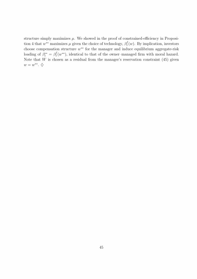
structure simply maximizes µ. We showed in the proof of constrained-efficiency in Proposi-

tion 4 that w∗∗ maximizes µ given the choice of technology, βf1 (w). By implication, investors

choose compensation structure w∗∗ for the manager and induce equilibrium aggregate-risk

loading of β∗∗1 = βf1 (w∗∗), identical to that of the owner–managed firm with moral hazard.

Note that W is chosen as a residual from the manager’s reservation constraint (45) given

w = w∗∗. ♦

45

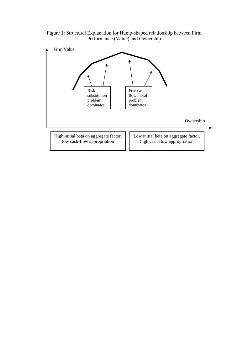
Figure 1: Structural Explanation for Hump-shaped relationship between Firm Performance (Value) and Ownership

Firm Value

Ownership

Risk-substitution problem dominates

Free cash-flow moral problem dominates

Low initial beta on aggregate factor, high cash-flow appropriation

High initial beta on aggregate factor, low cash-flow appropriation

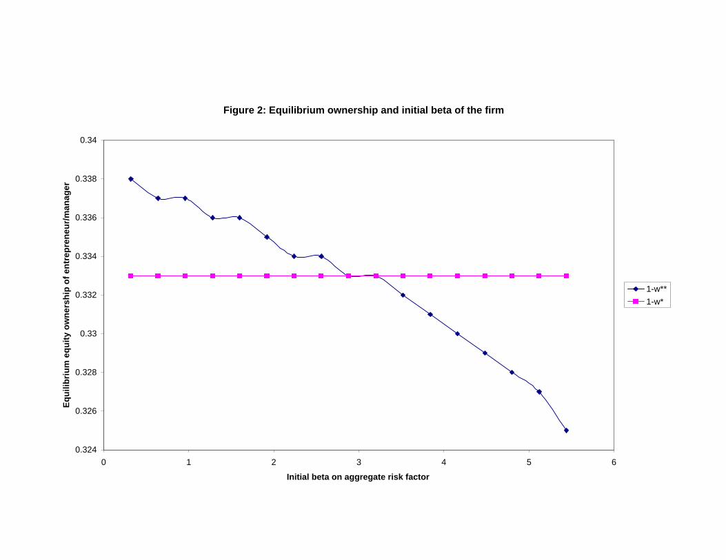
Figure 2: Equilibrium ownership and initial beta of the firm

0.324

0.326

0.328

0.33

0.332

0.334

0.336

0.338

0.34

0 1 2 3 4 5 6

Initial beta on aggregate risk factor

Equi

libriu

m e

quity

ow

ners

hip

of e

ntre

pren

eur/m

anag

er

1-w**1-w*

Figure 3: Equilibrium beta of the firm and endogenous equity ownership

0

1

2

3

4

5

6

0.324 0.326 0.328 0.33 0.332 0.334 0.336 0.338 0.34

Equilibrium equity ownership of entrepreneur/manager

Equi

libriu

m b

eta

on a

ggre

gate

risk

Eqm beta

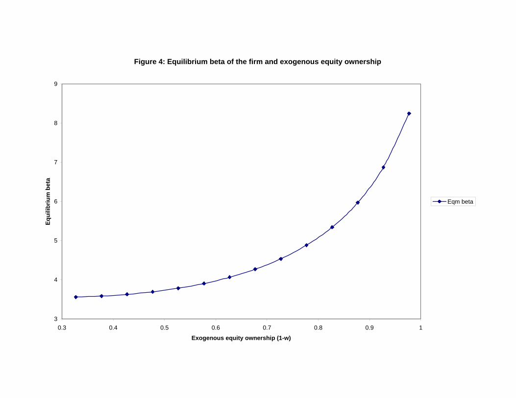
Figure 4: Equilibrium beta of the firm and exogenous equity ownership

3

4

5

6

7

8

9

0.3 0.4 0.5 0.6 0.7 0.8 0.9 1

Exogenous equity ownership (1-w)

Equi

libriu

m b

eta

Eqm beta

D Addendum: General Case of CAPM Economy and

Its Competitive Equilibrium

The economy is populated by H agents, F firms. Agent h’s preferences are represented

by a Constant Absolute Risk Aversion utility function uh(·) over the consumptions at date

0 and date 1, denoted as ch0 and ch

1 , respectively:

uh(ch0 , c

h1) ≡ −

1

Ae−Ach

0 − 1

Ae−Ach

1 . (D.1)

The economy has a N -dimensional orthogonal normal factor structure (x1, . . ., xn), which

is a multivariate normal with mean 0, and variance–covariance matrix (normalized to) I, the

identity matrix. In particular, each agent h’s endowments in period 1, yh1 , is generated as a

linear combination of N underlying normal risk factors, and hence is in general correlated

with other agents’ endowments:

yh1 − E(yh

1 ) ≡N∑

n=1

βhnxn , h = F + 1, ..., H. (D.2)

The first F < H agents are the entrepreneurs. Entrepreneur h owns the firm f(= h).

Each firm’s cash flow, yf1 , is also generated by the N factors. Without loss of generality,

we assume that the stock market risk is driven by C < N common orthogonal factors,

(x1, ..., xC), and F orthogonal factors, (xC+1, ..., xC+F ), which correspond to the sectoral risk

added by each firm’s cash flow:

yf1 − E(yf

1 ) ≡C∑

c=1

βfc xc + βf

f xC+f , f = 1, ..., F. (D.3)

Purely financial assets have payoff zi, i = 1, ..., I, which in terms of the factor structure

is written as

zi − E(zi) ≡C∑

c=1

βicxc +

I∑i=1

βijxC+F+i, i = 1, ..., I, (D.4)

where (xC+F+1, ..., xC+F+I) contains the additional risks in the return structure of financial

markets.

In our economy, all agents can trade the I financial assets and the C orthogonal factors.

Moreover, there exists a stock market for trade of the F firms, although the participation

46

of entrepreneurs (agents h ≤ F ) is restricted; in particular, entrepreneur f cannot trade

his own firm f , f = 1, . . . , F . Using the I financial assets, the C markets for factors, and

the market for the F stocks, under the assumptions of payoff orthogonality, agents can

replicate the payoffs of first C + F + I risk factors. (Participation restrictions in the stock

market translate into analogous participation restrictions in the market for the F firms’ risk

factors. Similarly, the positive net supply of stocks translates into positive net supply of all

factors.) Therefore it is formally equivalent, and it turns out to be convenient to represent

the competitive equilibrium of our CAPM economy in terms of not only the market but also

the prices of the C + F + I risk factors. We do this in the following.

We use a single index for all factors: j ∈ J ≡ 1, . . . , J, where J ≡ C + F + I. In

general, J < N , and the set of risky assets traded by agent h, denoted as J h, may be a

proper subset of J , that is, J h ⊂ J for some h, but we assume that all agents h are allowed

to trade the risk-free bond. Hj denotes the set of agents trading asset j, |Hj| being its size.

The problem of each agent h is to choose a consumption allocation at time 0, ch0 , portfolio

positions in the risk-free bond and in all tradable assets, [θh0 , θh

j ]j∈J , and a consumption

allocation at time 1, a random variable ch1 , to maximize the expected utility

E[uh(ch

0 , ch1)]≡ − 1

Ae−Ach

0 + E[− 1

Ae−Ach

1

], (D.5)

subject to the budget constraints and the restricted participation constraints:

ch0 = yh

0 − π0θh0 −

∑j∈J

πjθhj , h > F (D.6)

ch0 = yh

0 + whph − π0θh0 −

∑j∈J

πjθhj , h ∈ H, h ≤ F (D.7)

ch1 = yh

1 + θh0 +

∑j∈J

θhj xj, h > F (D.8)

ch1 = (1− wh)yh

1 + θh0 +

∑j∈J

θhj xj, h ≤ F (D.9)

θhj = 0, j 6∈ J h. (D.10)

Note that the budget constraint for entrepreneur h includes the time-0 proceeds from

the sale of a fraction wh of his firm amounting to whph. As discussed in the paper, under

rational expectations, the price of the firm ph is given by ph = π0E(yh1 ) +

∑1≤j≤J πjβ

hj . Let

shj denote the positive supply of risk factor j provided by the entrepreneur h through the

sale of fraction wh of his firm. Under the factor decomposition (equation D.3) for each firm’s

cash flows, these positive supplies are given by sh0 = whE(yh

1 ) and shj = whβh

j , 1 ≤ j ≤ J , so

that the proceeds from sale of the firm, whph, can also be expressed as whph =∑

0≤j≤J πjshj .

47

Definition D.1 A competitive equilibrium is a consumption allocation (ch0 , c

h1), for all agents

h ∈ H, which solves the problem of maximizing (D.5) subject to (D.6–D.10) at prices π ≡[π0, πj]j∈J , and such that consumption and financial markets clear

∑h

(ch0 − yh

0

)≤ 0, (D.11)

∑h

(ch1 − yh

1

)≤ 0, with probability 1 over Ω, and (D.12)

∑h

θhj = sj, j = 0, 1, . . . , J, (D.13)

where sj is the net supply of factor j, sj ≡∑

1≤h≤F shj .

Proposition D.2 The competitive equilibrium of the two-period CAPM economy, defined

by equations (D.5)–(D.10), with the market-clearing condition given by equations (D.11)–

(D.13), is characterized by prices of assets (πj), portfolio choices (θhj ), and consumption

allocations (cht ), given below.

π0 = exp

A (y0 − Ey1) +A2

2H

H∑h=1

(1−R2h)var(y

h1 ) +

∑j∈Jh

(βj +

1

|Hj|sj

)2 , (D.14)

where

y0 =1

H

H∑h=1

yh0 , y1 =

1

H

H∑h=1

yh1 , (D.15)

βj = cov

1

|Hj|

∑h∈Hj ,h≤F

(1− wh)yh1 +

∑h∈Hj ,h>F

yh1

, xj

, (D.16)

sh0 = whE(yh

1 ), shj = whβh

j , 1 ≤ j ≤ J, sj =∑

1≤h≤F

shj , 0 ≤ j ≤ J, (D.17)

πj

π0

= E (xj)− A

(βj +

1

|Hj|sj

), (D.18)

48

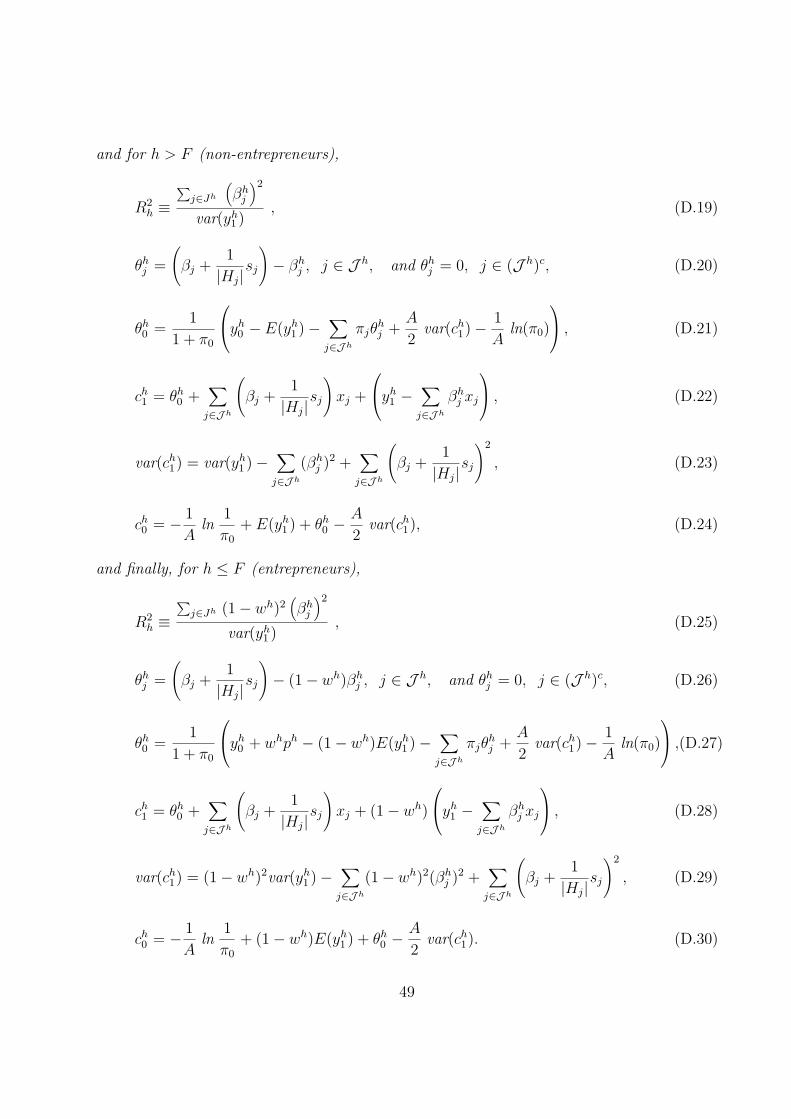
and for h > F (non-entrepreneurs),

R2h ≡

∑j∈Jh

(βh

j

)2

var(yh1 )

, (D.19)

θhj =

(βj +

1

|Hj|sj

)− βh

j , j ∈ J h, and θhj = 0, j ∈ (J h)c, (D.20)

θh0 =

1

1 + π0

yh0 − E(yh

1 )−∑

j∈J h

πjθhj +

A

2var(ch

1)−1

Aln(π0)

, (D.21)

ch1 = θh

0 +∑

j∈J h

(βj +

1

|Hj|sj

)xj +

yh1 −

∑j∈J h

βhj xj

, (D.22)

var(ch1) = var(yh

1 )−∑

j∈J h

(βhj )2 +

∑j∈J h

(βj +

1

|Hj|sj

)2

, (D.23)

ch0 = − 1

Aln

1

π0

+ E(yh1 ) + θh

0 −A

2var(ch

1), (D.24)

and finally, for h ≤ F (entrepreneurs),

R2h ≡

∑j∈Jh (1− wh)2

(βh

j

)2

var(yh1 )

, (D.25)

θhj =

(βj +

1

|Hj|sj

)− (1− wh)βh

j , j ∈ J h, and θhj = 0, j ∈ (J h)c, (D.26)

θh0 =

1

1 + π0

yh0 + whph − (1− wh)E(yh

1 )−∑

j∈J h

πjθhj +

A

2var(ch

1)−1

Aln(π0)

,(D.27)

ch1 = θh

0 +∑

j∈J h

(βj +

1

|Hj|sj

)xj + (1− wh)

yh1 −

∑j∈J h

βhj xj

, (D.28)

var(ch1) = (1− wh)2var(yh

1 )−∑

j∈J h

(1− wh)2(βhj )2 +

∑j∈J h

(βj +

1

|Hj|sj

)2

, (D.29)

ch0 = − 1

Aln

1

π0

+ (1− wh)E(yh1 ) + θh

0 −A

2var(ch

1). (D.30)

49

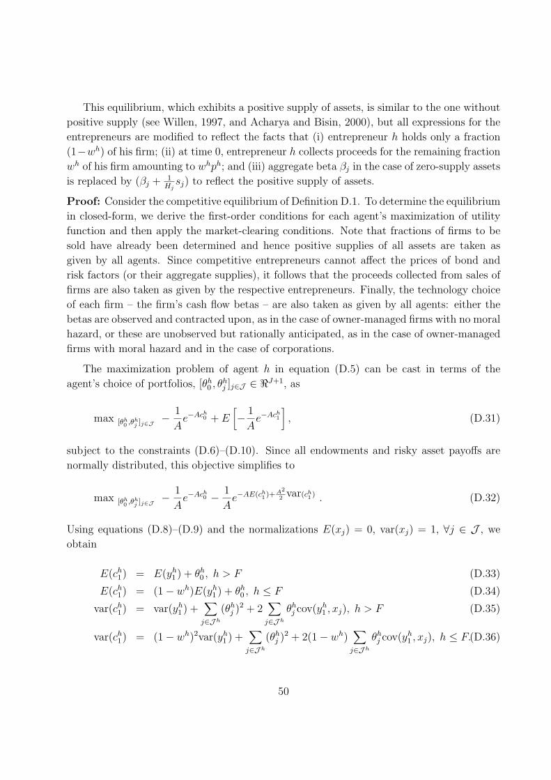
This equilibrium, which exhibits a positive supply of assets, is similar to the one without

positive supply (see Willen, 1997, and Acharya and Bisin, 2000), but all expressions for the

entrepreneurs are modified to reflect the facts that (i) entrepreneur h holds only a fraction

(1−wh) of his firm; (ii) at time 0, entrepreneur h collects proceeds for the remaining fraction

wh of his firm amounting to whph; and (iii) aggregate beta βj in the case of zero-supply assets

is replaced by (βj + 1Hj

sj) to reflect the positive supply of assets.

Proof: Consider the competitive equilibrium of Definition D.1. To determine the equilibrium

in closed-form, we derive the first-order conditions for each agent’s maximization of utility

function and then apply the market-clearing conditions. Note that fractions of firms to be

sold have already been determined and hence positive supplies of all assets are taken as

given by all agents. Since competitive entrepreneurs cannot affect the prices of bond and

risk factors (or their aggregate supplies), it follows that the proceeds collected from sales of

firms are also taken as given by the respective entrepreneurs. Finally, the technology choice

of each firm – the firm’s cash flow betas – are also taken as given by all agents: either the

betas are observed and contracted upon, as in the case of owner-managed firms with no moral

hazard, or these are unobserved but rationally anticipated, as in the case of owner-managed

firms with moral hazard and in the case of corporations.

The maximization problem of agent h in equation (D.5) can be cast in terms of the

agent’s choice of portfolios, [θh0 , θh

j ]j∈J ∈ <J+1, as

max [θh0 ,θh

j ]j∈J− 1

Ae−Ach

0 + E[− 1

Ae−Ach

1

], (D.31)

subject to the constraints (D.6)–(D.10). Since all endowments and risky asset payoffs are

normally distributed, this objective simplifies to

max [θh0 ,θh

j ]j∈J− 1

Ae−Ach

0 − 1

Ae−AE(ch

1 )+A2

2var(ch

1 ) . (D.32)

Using equations (D.8)–(D.9) and the normalizations E(xj) = 0, var(xj) = 1, ∀j ∈ J , we

obtain

E(ch1) = E(yh

1 ) + θh0 , h > F (D.33)

E(ch1) = (1− wh)E(yh

1 ) + θh0 , h ≤ F (D.34)

var(ch1) = var(yh

1 ) +∑

j∈J h

(θhj )2 + 2

∑j∈J h

θhj cov(yh

1 , xj), h > F (D.35)

var(ch1) = (1− wh)2var(yh

1 ) +∑

j∈J h

(θhj )2 + 2(1− wh)

∑j∈J h

θhj cov(yh

1 , xj), h ≤ F.(D.36)

50

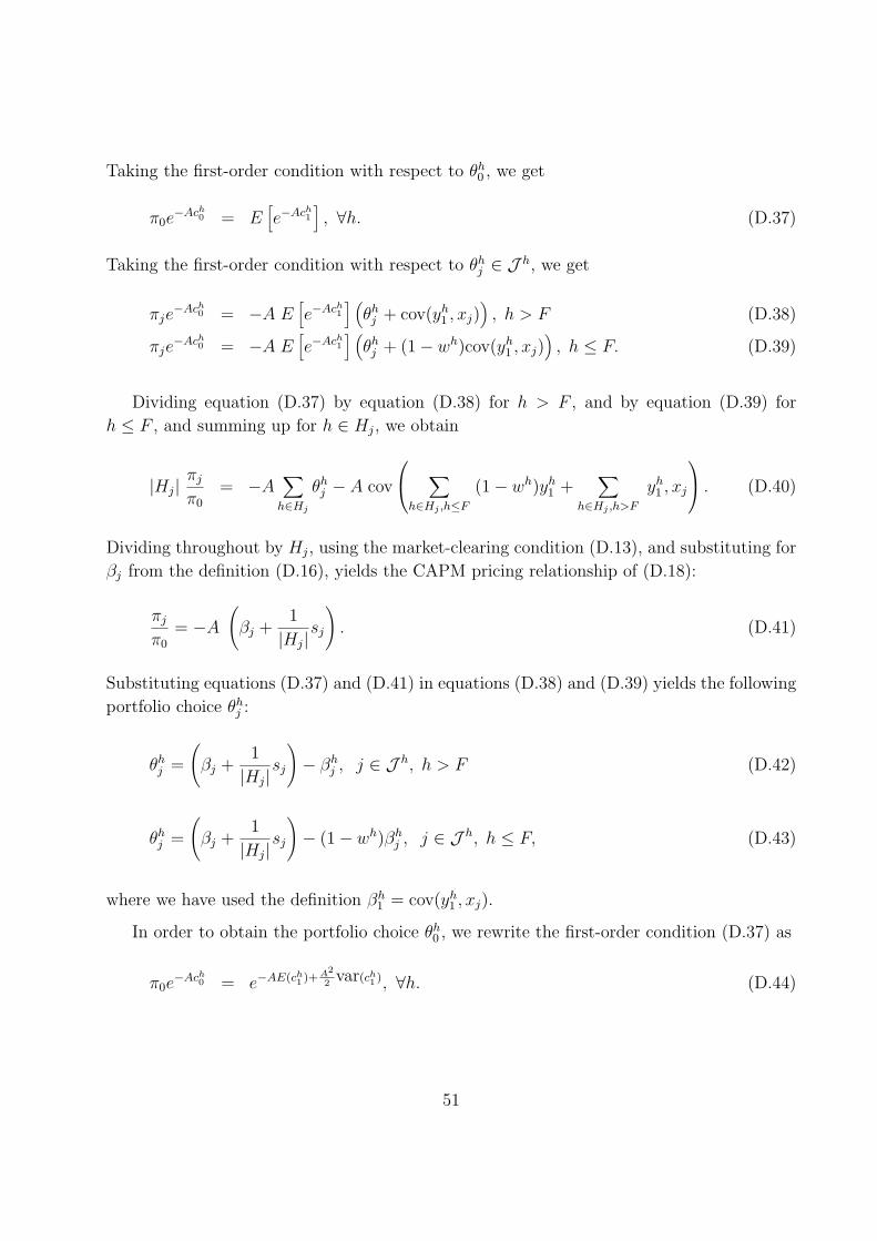
Taking the first-order condition with respect to θh0 , we get

π0e−Ach

0 = E[e−Ach

1

], ∀h. (D.37)

Taking the first-order condition with respect to θhj ∈ J h, we get

πje−Ach

0 = −A E[e−Ach

1

] (θh

j + cov(yh1 , xj)

), h > F (D.38)

πje−Ach

0 = −A E[e−Ach

1

] (θh

j + (1− wh)cov(yh1 , xj)

), h ≤ F. (D.39)

Dividing equation (D.37) by equation (D.38) for h > F , and by equation (D.39) for

h ≤ F , and summing up for h ∈ Hj, we obtain

|Hj|πj

π0

= −A∑

h∈Hj

θhj − A cov

∑h∈Hj ,h≤F

(1− wh)yh1 +

∑h∈Hj ,h>F

yh1 , xj

. (D.40)

Dividing throughout by Hj, using the market-clearing condition (D.13), and substituting for

βj from the definition (D.16), yields the CAPM pricing relationship of (D.18):

πj

π0

= −A

(βj +

1

|Hj|sj

). (D.41)

Substituting equations (D.37) and (D.41) in equations (D.38) and (D.39) yields the following

portfolio choice θhj :

θhj =

(βj +

1

|Hj|sj

)− βh

j , j ∈ J h, h > F (D.42)

θhj =

(βj +

1

|Hj|sj

)− (1− wh)βh

j , j ∈ J h, h ≤ F, (D.43)

where we have used the definition βh1 = cov(yh

1 , xj).

In order to obtain the portfolio choice θh0 , we rewrite the first-order condition (D.37) as

π0e−Ach

0 = e−AE(ch1 )+A2

2var(ch

1 ), ∀h. (D.44)

51

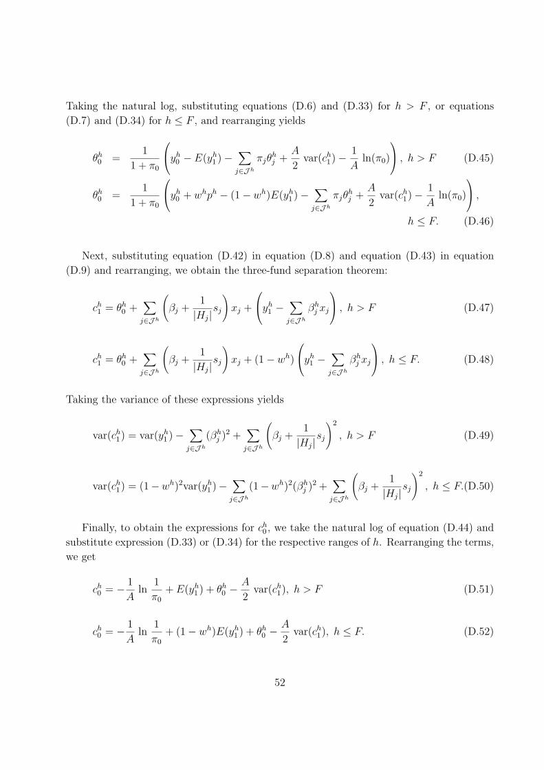
Taking the natural log, substituting equations (D.6) and (D.33) for h > F , or equations

(D.7) and (D.34) for h ≤ F , and rearranging yields

θh0 =

1

1 + π0

yh0 − E(yh

1 )−∑

j∈J h

πjθhj +

A

2var(ch

1)−1

Aln(π0)

, h > F (D.45)

θh0 =

1

1 + π0

yh0 + whph − (1− wh)E(yh

1 )−∑

j∈J h

πjθhj +

A

2var(ch

1)−1

Aln(π0)

,

h ≤ F. (D.46)

Next, substituting equation (D.42) in equation (D.8) and equation (D.43) in equation

(D.9) and rearranging, we obtain the three-fund separation theorem:

ch1 = θh

0 +∑

j∈J h

(βj +

1

|Hj|sj

)xj +

yh1 −

∑j∈J h

βhj xj

, h > F (D.47)

ch1 = θh

0 +∑

j∈J h

(βj +

1

|Hj|sj

)xj + (1− wh)

yh1 −

∑j∈J h

βhj xj

, h ≤ F. (D.48)

Taking the variance of these expressions yields

var(ch1) = var(yh

1 )−∑

j∈J h

(βhj )2 +

∑j∈J h

(βj +

1

|Hj|sj

)2

, h > F (D.49)

var(ch1) = (1−wh)2var(yh

1 )−∑

j∈J h

(1−wh)2(βhj )2 +

∑j∈J h

(βj +

1

|Hj|sj

)2

, h ≤ F.(D.50)

Finally, to obtain the expressions for ch0 , we take the natural log of equation (D.44) and

substitute expression (D.33) or (D.34) for the respective ranges of h. Rearranging the terms,

we get

ch0 = − 1

Aln

1

π0

+ E(yh1 ) + θh

0 −A

2var(ch

1), h > F (D.51)

ch0 = − 1

Aln

1

π0

+ (1− wh)E(yh1 ) + θh

0 −A

2var(ch

1), h ≤ F. (D.52)

52

Now, all equilibrium quantities are determined in terms of the risk-free asset’s price, π0. To

determine this, we take the natural log of equation (D.44) and sum over all agents to obtain

H ln(π0)− AH∑

h=1

yh0 = −A

H∑h=1

E(yh1 ) +

A2

2

H∑h=1

var(ch1). (D.53)

Dividing throughout by H, using the definitions for mean endowments y0 and y1 in equation

(D.15), and substituting for var(ch1) from equations (D.23) and (D.29), π0 can be determined

in terms of the model’s primitive quantities as follows:

π0 = exp

A (y0 − Ey1) +A2

2H

H∑h=1

(1−R2h)var(yh

1 ) +∑

j∈Jh

(βj +

1

|Hj|sj

)2 , (D.54)

where

R2h ≡

∑j∈Jh

(βh

j

)2

var(yh1 )

, h > F, and R2h ≡

∑j∈Jh (1− wh)2

(βh

j

)2

var(yh1 )

, h ≤ F (D.55)

represent the variability of agent h’s endowment that is spanned by the risky assets tradable

by the agent.

The competitive equilibrium is now fully determined in closed-form once the supply

conditions are substituted:

sh0 = whE(yh

1 ), shj = whβh

j , 1 ≤ j ≤ J, sj =∑

1≤h≤F

shj , 0 ≤ j ≤ J . ♦ (D.56)

53