Copyright © 2010 by the McGraw-Hill Companies, Inc. All rights reserved.McGraw-Hill/Irwin

Managerial Economics & Business Strategy

Chapter 5The Production

Process and Costs

5-2

Overview

I. Production Analysis– Total Product, Marginal Product, Average Product.– Isoquants.– Isocosts.– Cost Minimization

II. Cost Analysis– Total Cost, Variable Cost, Fixed Costs.– Cubic Cost Function.– Cost Relations.

III. Multi-Product Cost Functions

5-3

Production Analysis Production Function

– Q = F(K,L)• Q is quantity of output produced.• K is capital input.• L is labor input.• F is a functional form relating the inputs to output.

– The maximum amount of output that can be produced with K units of capital and L units of labor.

Short-Run vs. Long-Run Decisions Fixed vs. Variable Inputs

5-4

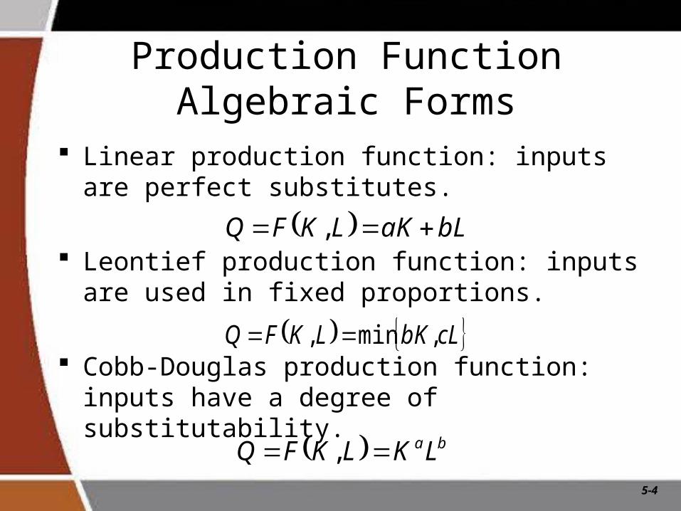
Production Function Algebraic Forms

Linear production function: inputs are perfect substitutes.

Leontief production function: inputs are used in fixed proportions.

Cobb-Douglas production function: inputs have a degree of substitutability.

ba LKLKFQ ,

bLaKLKFQ ,

cLbKLKFQ ,min,

5-5

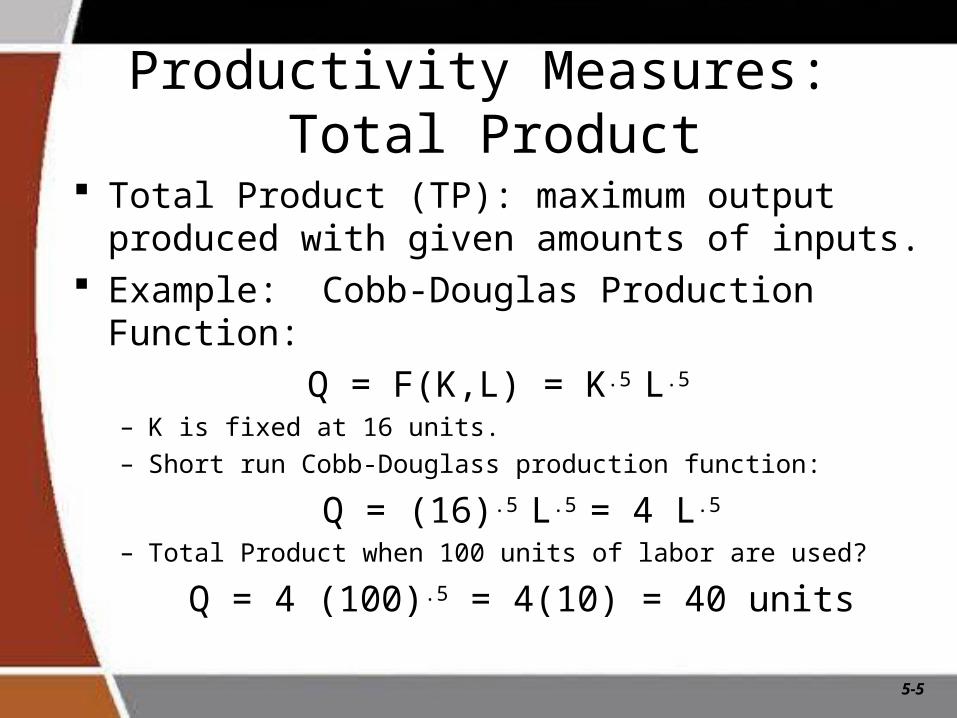
Productivity Measures: Total Product

Total Product (TP): maximum output produced with given amounts of inputs.

Example: Cobb-Douglas Production Function:

Q = F(K,L) = K.5 L.5

– K is fixed at 16 units. – Short run Cobb-Douglass production function:

Q = (16).5 L.5 = 4 L.5

– Total Product when 100 units of labor are used?

Q = 4 (100).5 = 4(10) = 40 units

5-6

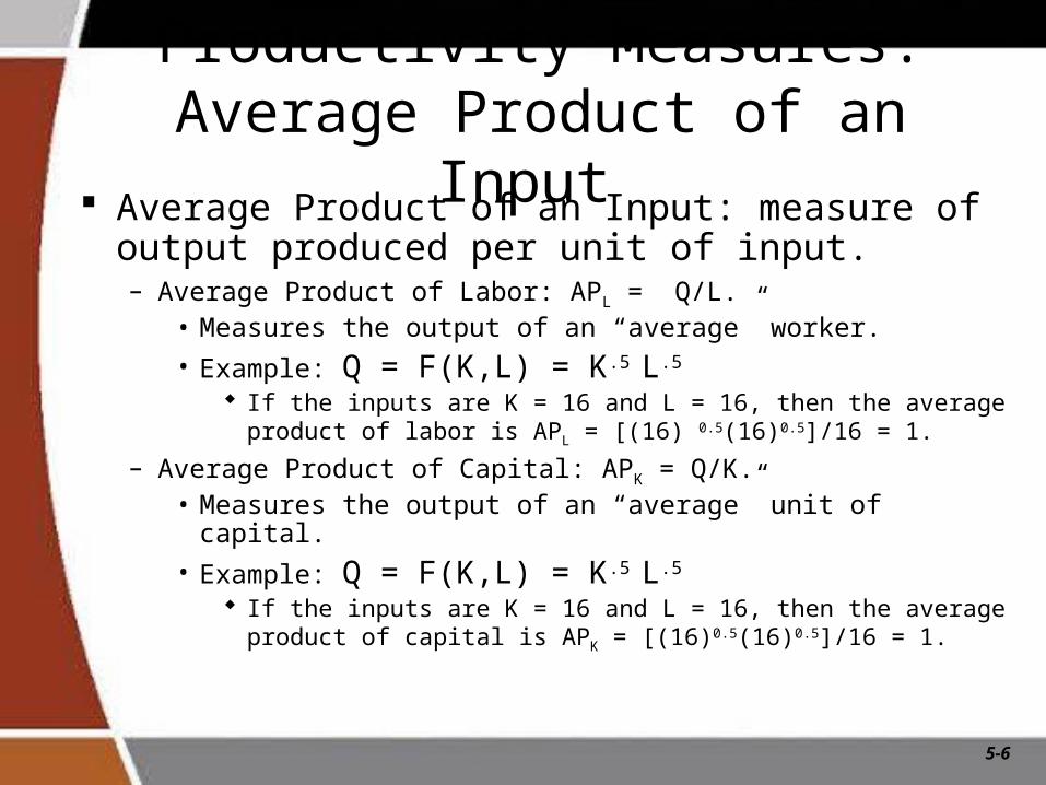
Productivity Measures: Average Product of an Input

Average Product of an Input: measure of output produced per unit of input.– Average Product of Labor: APL = Q/L.

• Measures the output of an “average” worker.

• Example: Q = F(K,L) = K.5 L.5

If the inputs are K = 16 and L = 16, then the average product of labor is APL = [(16) 0.5(16)0.5]/16 = 1.

– Average Product of Capital: APK = Q/K.• Measures the output of an “average” unit of capital.

• Example: Q = F(K,L) = K.5 L.5

If the inputs are K = 16 and L = 16, then the average product of capital is APK = [(16)0.5(16)0.5]/16 = 1.

5-7

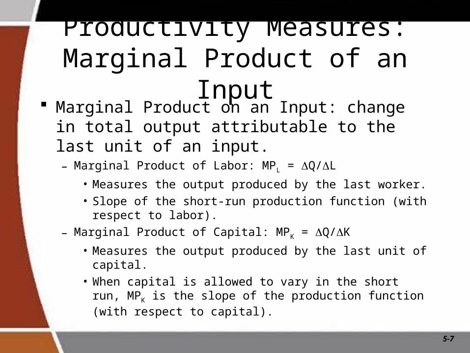
Productivity Measures: Marginal Product of an Input

Marginal Product on an Input: change in total output attributable to the last unit of an input.– Marginal Product of Labor: MPL = Q/L

• Measures the output produced by the last worker.• Slope of the short-run production function (with respect

to labor).

– Marginal Product of Capital: MPK = Q/K

• Measures the output produced by the last unit of capital.

• When capital is allowed to vary in the short run, MPK is the slope of the production function (with respect to capital).

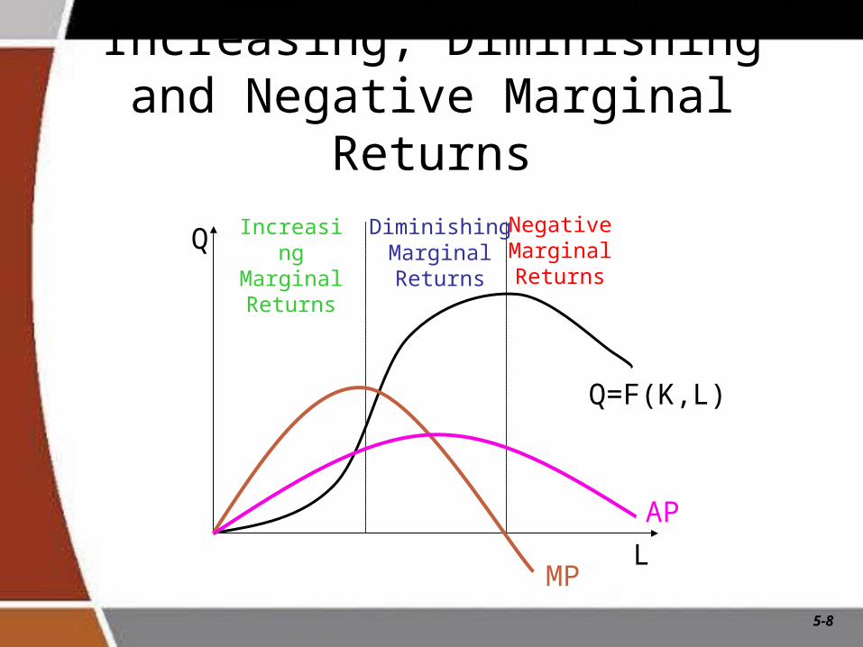
5-8

Q

L

Q=F(K,L)

IncreasingMarginalReturns

DiminishingMarginalReturns

NegativeMarginalReturns

MP

AP

Increasing, Diminishing and Negative Marginal Returns

5-9

Guiding the Production Process

Producing on the production function– Aligning incentives to induce maximum worker

effort. Employing the right level of inputs

– When labor or capital vary in the short run, to maximize profit a manager will hire:

• labor until the value of marginal product of labor equals the wage: VMPL = w, where VMPL = P x MPL.

• capital until the value of marginal product of capital equals the rental rate: VMPK = r, where VMPK = P x MPK .

5-10

Isoquant

Illustrates the long-run combinations of inputs (K, L) that yield the producer the same level of output.

The shape of an isoquant reflects the ease with which a producer can substitute among inputs while maintaining the same level of output.

5-11

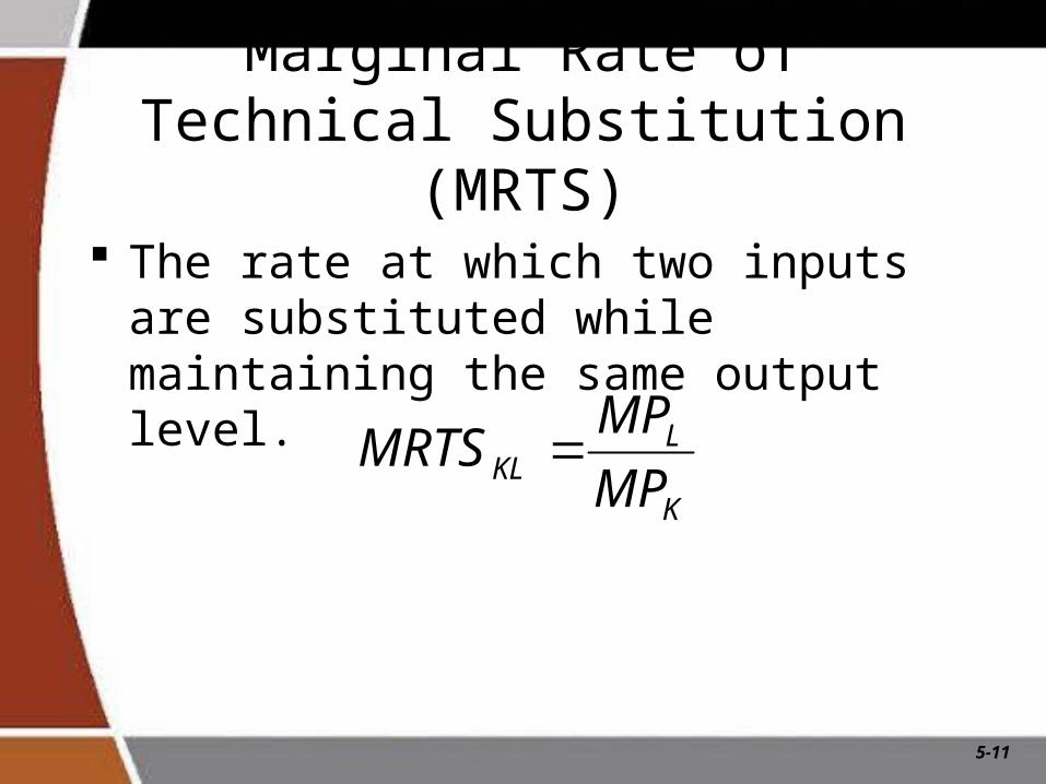
Marginal Rate of Technical Substitution (MRTS)

The rate at which two inputs are substituted while maintaining the same output level.

K

LKL MP

MPMRTS

5-12

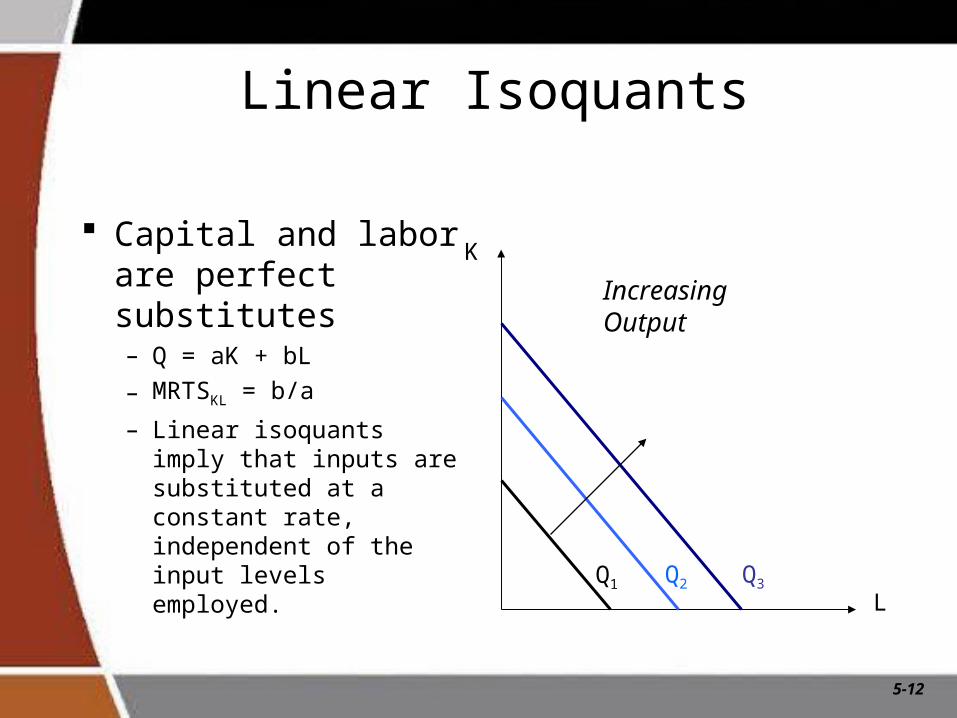
Linear Isoquants

Capital and labor are perfect substitutes– Q = aK + bL

– MRTSKL = b/a

– Linear isoquants imply that inputs are substituted at a constant rate, independent of the input levels employed. Q3Q2Q1

Increasing Output

L

K

5-13

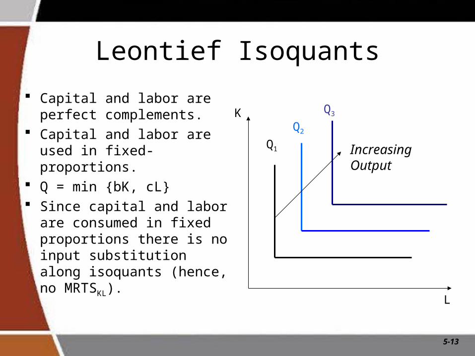
Leontief Isoquants

Capital and labor are perfect complements.

Capital and labor are used in fixed-proportions.

Q = min {bK, cL} Since capital and labor are

consumed in fixed proportions there is no input substitution along isoquants (hence, no MRTSKL).

Q3

Q2

Q1

K

Increasing Output

L

5-14

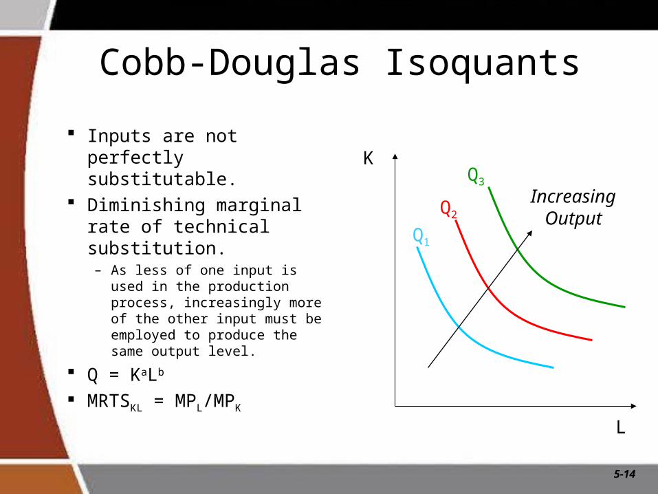
Cobb-Douglas Isoquants

Inputs are not perfectly substitutable.

Diminishing marginal rate of technical substitution.– As less of one input is used in

the production process, increasingly more of the other input must be employed to produce the same output level.

Q = KaLb

MRTSKL = MPL/MPK

Q1

Q2

Q3

K

L

Increasing Output

5-15

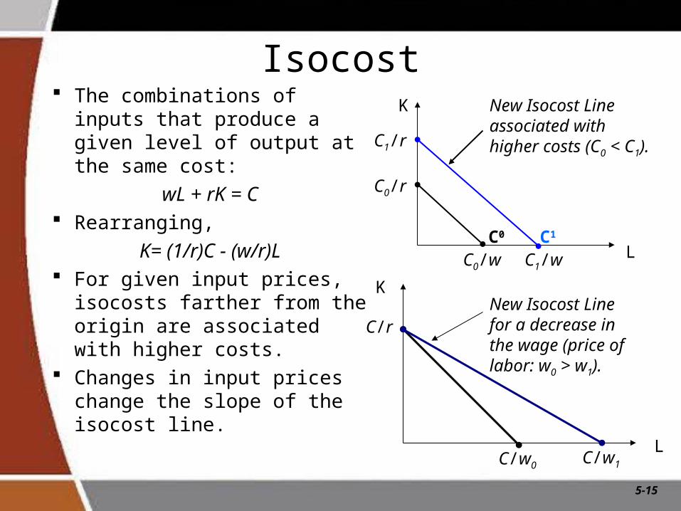
Isocost The combinations of inputs

that produce a given level of output at the same cost:

wL + rK = C Rearranging,

K= (1/r)C - (w/r)L For given input prices,

isocosts farther from the origin are associated with higher costs.

Changes in input prices change the slope of the isocost line.

K

LC1

L

KNew Isocost Line for a decrease in the wage (price of labor: w0 > w1).

C1/r

C1/wC0

C0/w

C0/r

C/w0 C/w1

C/r

New Isocost Line associated with higher costs (C0 < C1).

5-16

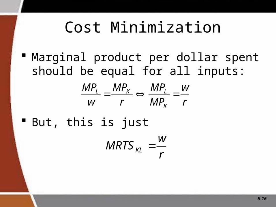
Cost Minimization

Marginal product per dollar spent should be equal for all inputs:

But, this is just

r

w

MP

MP

r

MP

w

MP

K

LKL

r

wMRTSKL

5-17

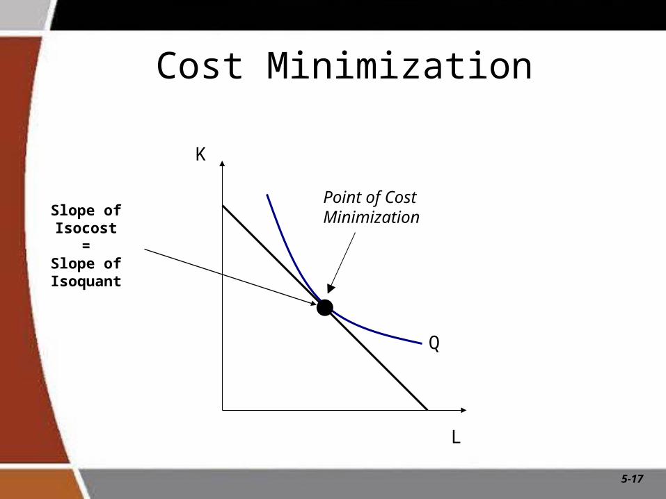
Cost Minimization

Q

L

K

Point of Cost Minimization

Slope of Isocost =

Slope of Isoquant

5-18

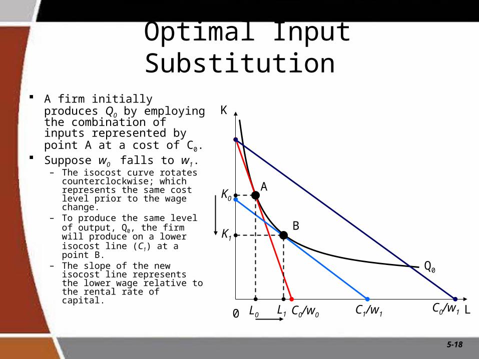
Optimal Input Substitution

A firm initially produces Q0 by employing the combination of inputs represented by point A at a cost of C0.

Suppose w0 falls to w1.– The isocost curve rotates

counterclockwise; which represents the same cost level prior to the wage change.

– To produce the same level of output, Q0, the firm will produce on a lower isocost line (C1) at a point B.

– The slope of the new isocost line represents the lower wage relative to the rental rate of capital.

Q0

0

A

L

K

C0/w1C0/w0 C1/w1L0 L1

K0

K1

B

5-19

Cost Analysis

Types of Costs– Short-Run

• Fixed costs (FC)• Sunk costs • Short-run variable

costs (VC)• Short-run total costs

(TC)– Long-Run

• All costs are variable

• No fixed costs

5-20

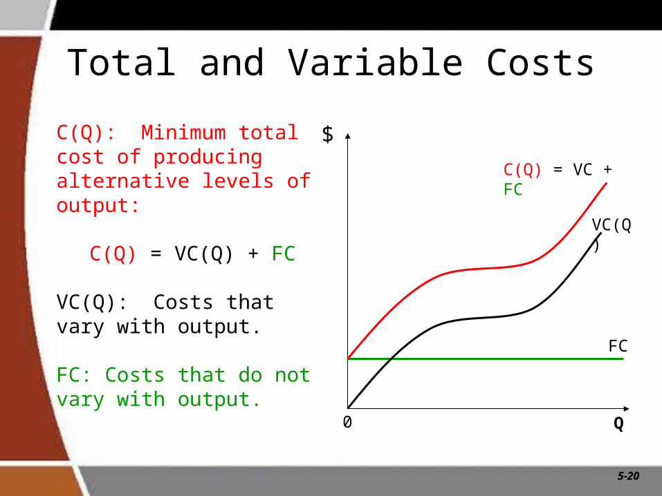
Total and Variable Costs

C(Q): Minimum total cost of producing alternative levels of output:

C(Q) = VC(Q) + FC

VC(Q): Costs that vary with output.

FC: Costs that do not vary with output.

$

Q

C(Q) = VC + FC

VC(Q)

FC

0

5-21

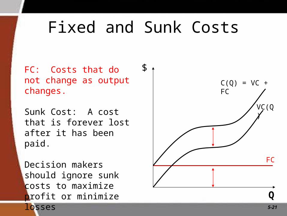
Fixed and Sunk Costs

FC: Costs that do not change as output changes.

Sunk Cost: A cost that is forever lost after it has been paid.

Decision makers should ignore sunk costs to maximize profit or minimize losses

$

Q

FC

C(Q) = VC + FC

VC(Q)

5-22

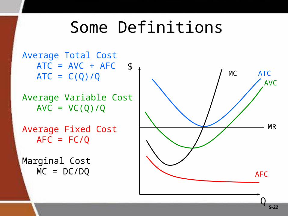
Some Definitions

Average Total CostATC = AVC + AFCATC = C(Q)/Q

Average Variable CostAVC = VC(Q)/Q

Average Fixed CostAFC = FC/Q

Marginal CostMC = DC/DQ

$

Q

ATCAVC

AFC

MC

MR

5-23

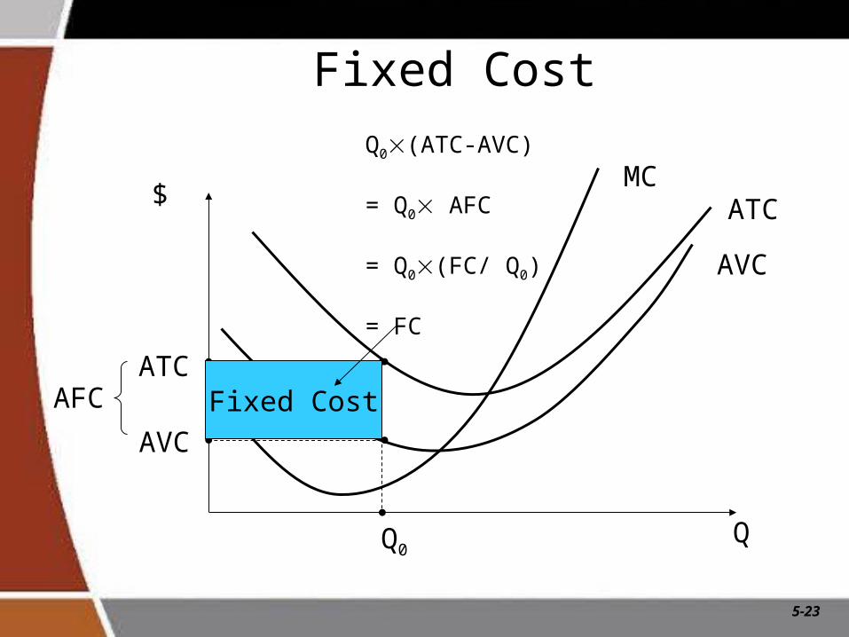
Fixed Cost

$

Q

ATC

AVC

MC

ATC

AVC

Q0

AFC Fixed Cost

Q0(ATC-AVC)

= Q0 AFC

= Q0(FC/ Q0)

= FC

5-24

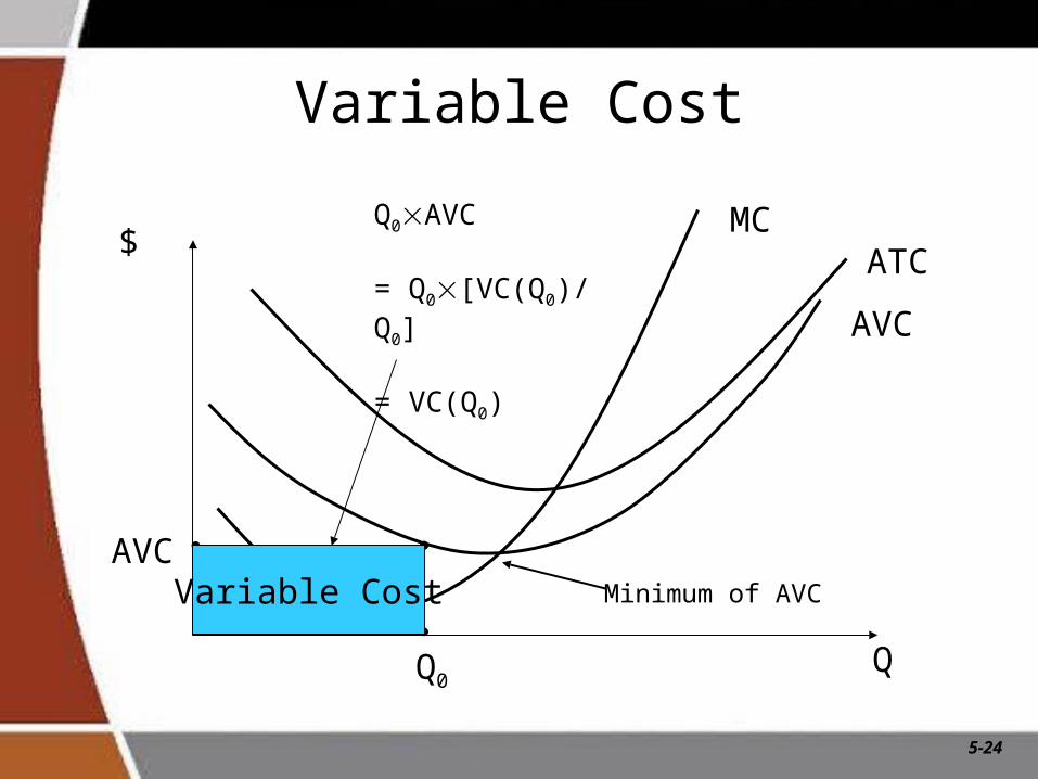
Variable Cost

$

Q

ATC

AVC

MC

AVCVariable Cost

Q0

Q0AVC

= Q0[VC(Q0)/ Q0]

= VC(Q0)

Minimum of AVC

5-25

$

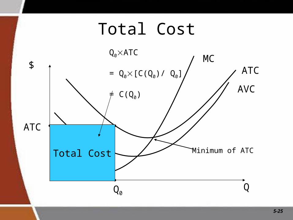
Q

ATC

AVC

MC

ATC

Total Cost

Q0

Q0ATC

= Q0[C(Q0)/ Q0]

= C(Q0)

Total Cost

Minimum of ATC

5-26

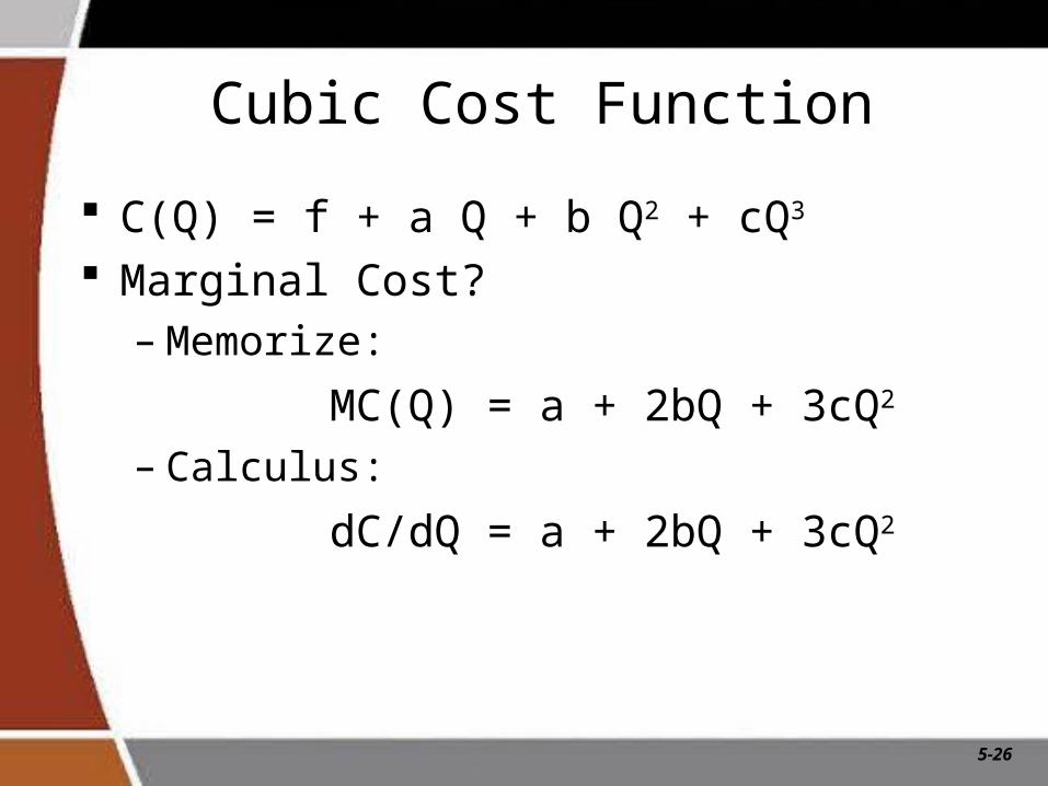
Cubic Cost Function

C(Q) = f + a Q + b Q2 + cQ3

Marginal Cost?– Memorize:

MC(Q) = a + 2bQ + 3cQ2

– Calculus:

dC/dQ = a + 2bQ + 3cQ2

5-27

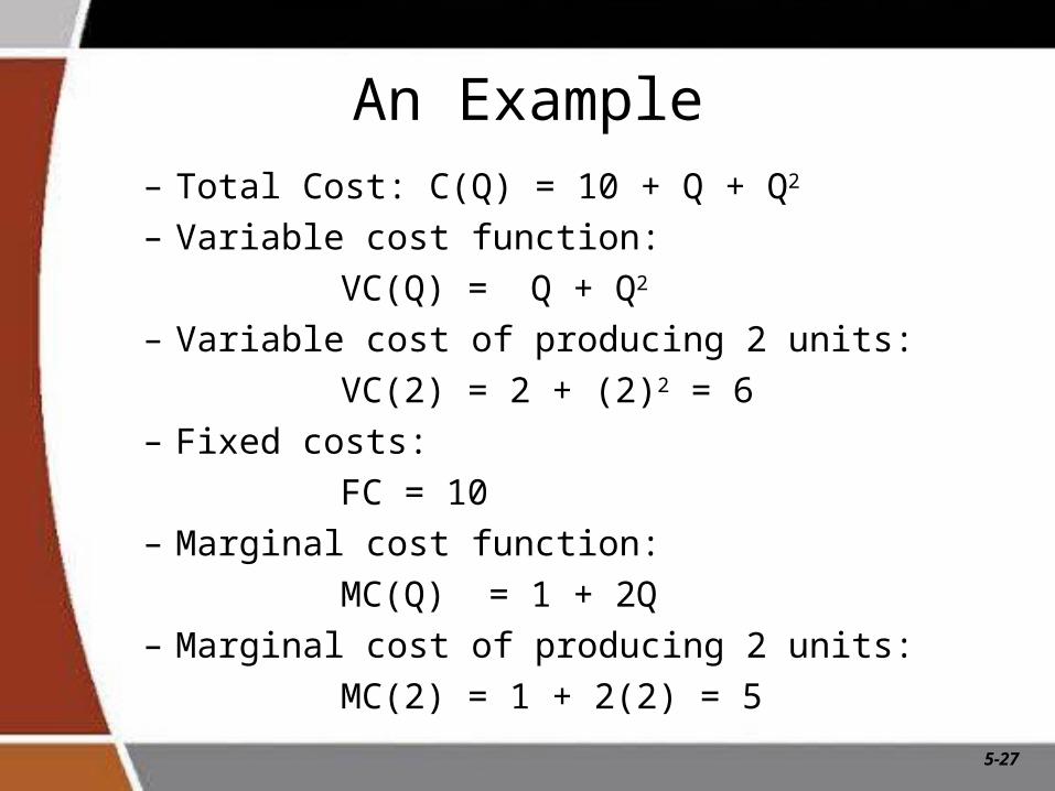
An Example– Total Cost: C(Q) = 10 + Q + Q2

– Variable cost function:

VC(Q) = Q + Q2

– Variable cost of producing 2 units:

VC(2) = 2 + (2)2 = 6– Fixed costs:

FC = 10– Marginal cost function:

MC(Q) = 1 + 2Q– Marginal cost of producing 2 units:

MC(2) = 1 + 2(2) = 5

5-28

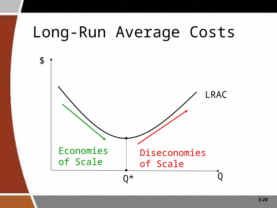
Long-Run Average Costs

LRAC

$

Q

Economiesof Scale

Diseconomiesof Scale

Q*

5-29

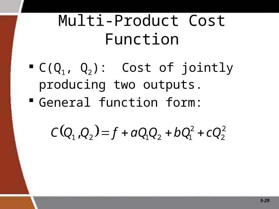
Multi-Product Cost Function

C(Q1, Q2): Cost of jointly producing two outputs.

General function form:

22

212121, cQbQQaQfQQC

5-30

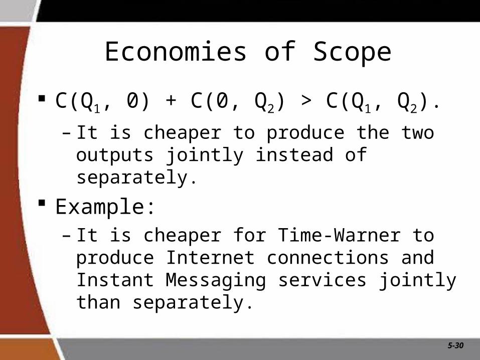
Economies of Scope

C(Q1, 0) + C(0, Q2) > C(Q1, Q2).

– It is cheaper to produce the two outputs jointly instead of separately.

Example:– It is cheaper for Time-Warner to produce

Internet connections and Instant Messaging services jointly than separately.

5-31

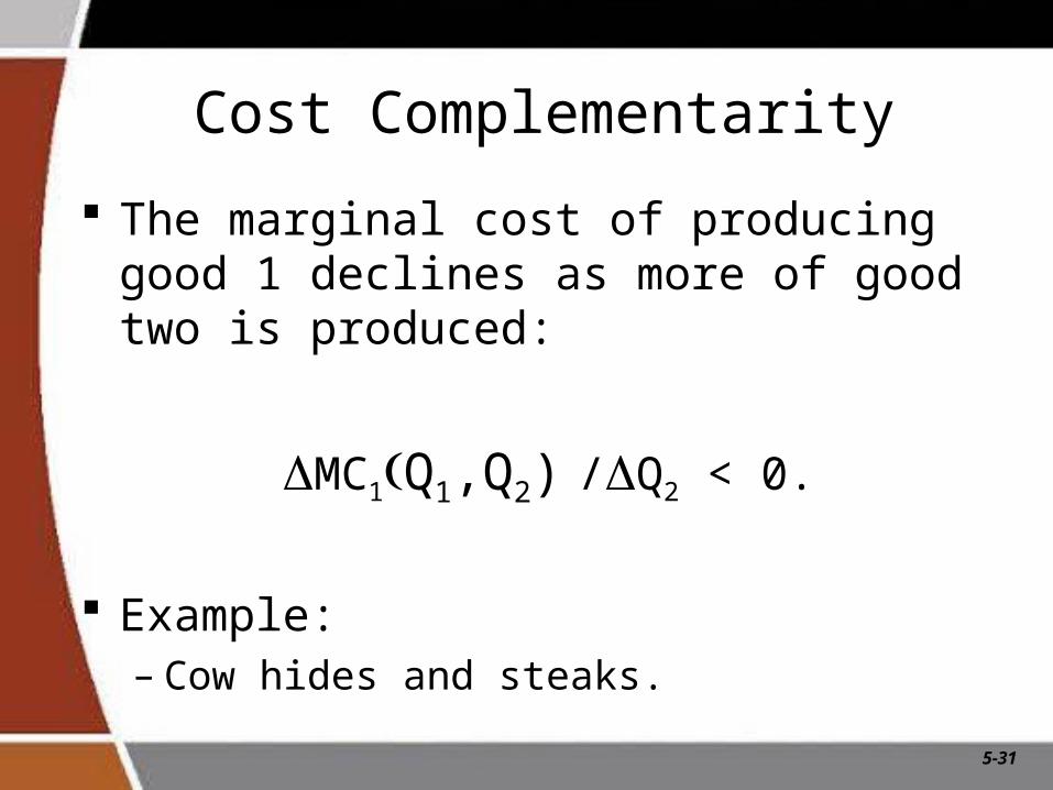
Cost Complementarity

The marginal cost of producing good 1 declines as more of good two is produced:

MC1Q1,Q2) /Q2 < 0.

Example:– Cow hides and steaks.

5-32

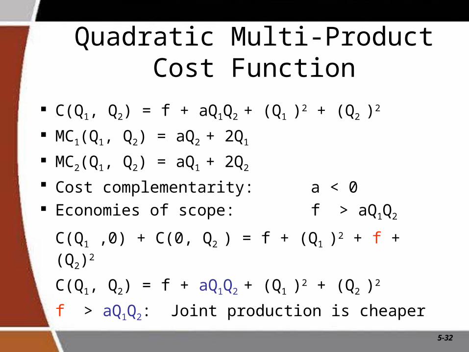
Quadratic Multi-Product Cost Function

C(Q1, Q2) = f + aQ1Q2 + (Q1 )2 + (Q2 )2

MC1(Q1, Q2) = aQ2 + 2Q1

MC2(Q1, Q2) = aQ1 + 2Q2

Cost complementarity: a < 0 Economies of scope: f > aQ1Q2

C(Q1 ,0) + C(0, Q2 ) = f + (Q1 )2 + f + (Q2)2

C(Q1, Q2) = f + aQ1Q2 + (Q1 )2 + (Q2 )2

f > aQ1Q2: Joint production is cheaper

5-33

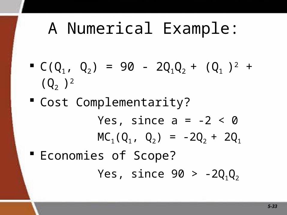
A Numerical Example:

C(Q1, Q2) = 90 - 2Q1Q2 + (Q1 )2 + (Q2 )2

Cost Complementarity?

Yes, since a = -2 < 0

MC1(Q1, Q2) = -2Q2 + 2Q1

Economies of Scope?

Yes, since 90 > -2Q1Q2

5-34

Conclusion

To maximize profits (minimize costs) managers must use inputs such that the value of marginal of each input reflects price the firm must pay to employ the input.

The optimal mix of inputs is achieved when the MRTSKL = (w/r).

Cost functions are the foundation for helping to determine profit-maximizing behavior in future chapters.