MANAGEMENT AS A TECHNOLOGY?∗

Nicholas Bloom (Stanford), Raffaella Sadun (Harvard) and John Van Reenen (LSE)

May 31, 2016

Abstract

Are some management practices akin to a technology that can explain company and national

productivity, or do they simply reflect contingent management styles? We collect data on core

management practices from over 11,000 firms in 34 countries. We find large cross-country

differences in the adoption of basic management practices, with the US having the highest

size-weighted average management score. We present a formal model of “Management as a

Technology”, and structurally estimate it using panel data to recover parameters including the

depreciation rate and adjustment costs of managerial capital (both found to be larger than for

tangible non-managerial capital). Our model also predicts (i) a positive effect of management on

firm performance; (ii) a positive relationship between product market competition and average

management quality (part of which stems from the larger covariance between management

with firm size as competition strengthens); and (iii) a rise (fall) in the level (dispersion) of

management with firm age. We find strong empirical support for all of these predictions in our

data. Finally, building on our model, we find that differences in management practices account

for about 30% of cross-country total factor productivity differences.

JEL No. L2, M2, O32, O33.

Keywords: management practices, productivity, competition

∗Acknowledgments: We would like to thank Orazio Attanasio, Marianne Bertrand, Robert Gibbons, John Halti-wanger, Rebecca Henderson, Bengt Holmstrom, Michael Peters and Michele Tertilt for helpful comments as well asparticipants in seminars at the AEA, Barcelona, Berkeley, Birmingham, Bocconi, Brussels, CEU, Chicago, Dublin,Duke, Essex, George Washington, Harvard, Hong Kong, IIES, LBS, Leuven, LSE, Madrid, Mannheim, Michigan,Minnesota, MIT, Munich, Naples, NBER, NYU, Peterson, Princeton, Stockholm, Sussex, Toronto, Uppsala, USC,Yale and Zurich. The Economic and Social Research Council, the Kauffman Foundation, PEDL and the Alfred SloanFoundation have given financial support. We received no funding from the global management consultancy firm(McKinsey) we worked with in developing the survey tool. Our partnership with Pedro Castro, Stephen Dorgan andJohn Dowdy has been particularly important in the development of the project. We are grateful to Daniela Scur andRenata Lemos for ongoing discussion and feedback on the paper.

1

1 Introduction

Productivity differences between firms and between countries remain startling. For example, within

the average four-digit U.S. manufacturing industries, Syverson (2011) finds that labor productivity

for plants at the 90th percentile was four times as high as plants at the 10th percentile. Even after

controlling for other factors, Total Factor Productivity (TFP) was almost twice as high. These

differences persist over time and are robust to controlling for plant-specific prices in homogeneous

goods industries.1 Such TFP heterogeneity is evident in all other countries where data is available.2

One explanation is that these persistent within industry productivity differentials are due to “hard”

technological innovations, as embodied in patents or the adoption of advanced equipment. Another

explanation, which is the focus of this paper, is that productivity differences reflect variations in

management practices.

We advance the idea that some forms of management practices are like a “technology”, in the sense

that they raise TFP. This has a number of empirical implications that we examine and find support

for in the data. Our perspective on management is distinct from the dominant “Design” paradigm

in organizational economics, which views management as a question of optimal design depending

on the contingent features of a firm’s environment (Gibbons and Roberts, 2013). In this contingent

view of management practices, there is no sense in which any management styles are on average

better than any others. Our data provides some support for Design perspective, but we show that

- at least within the very stylized version of this perspective that we consider - this delivers only a

partial explanation of the patterns that we can observe in our data.

To date, empirical work to measure differences in management practices across firms and countries

has been limited. Despite this lack of data, the core theories in many fields such as international

trade, labor economics, industrial organization and macroeconomics are now incorporating firm

heterogeneity as a central component.3

To address the lack of management data, we collect original survey data on management practices

on over 11,000 firms in 34 countries. Besides its rich cross sectional nature, both in terms of

countries and industries covered, this dataset also features a significant panel component built

through four different survey waves from 2004 to 2014. We first present some stylized facts from

this database in the cross country and cross firm dimensions. One of the striking features of the

1These are revenue based measures of TFP (“TFPR”) so will also reflect firm-specific mark-ups. Foster, Halti-wanger and Syverson (2008) show large differences in TFP even within very homogeneous goods industries suchas cement and block ice. Hall and Jones (1999) and Jones and Romer (2010) show how the stark differences inproductivity across countries account for a substantial fraction of the differences in average income.

2Usually productivity dispersion is even greater than in other countries than in the U.S. - see Bartelsman, Halti-wanger and Scarpetta (2013) and Hsieh and Klenow (2009).

3Different fields have different labels for management. In trade, the focus is on an initial productivity draw whenthe plant enters an industry that persists over time (e.g. Melitz, 2003). In industrial organization, the focus hastraditionally been on cost heterogeneity due to entrepreneurial/managerial talent (e.g. Lucas, 1978). In macro,organizational capital is sometimes related to the firm specific managerial know-how built up over time (e.g. Prescottand Visscher 1980). In labor, there is a growing focus on how the wage distribution requires an understanding of theheterogeneity of firm productivity (e.g. Card, Heining and Kline, 2013).

2

data is that the average management score, just like TFP, is higher in the U.S. than it is in other

countries (see Figure 1). A second striking feature - shown in Figure 2 - is that management, like

TFP, shows a wide dispersion across firms within each country. Interestingly, this dispersion is

lower in countries like the U.S. with lower levels of market frictions than it is in countries like India

and Brazil.

We detail a simple model of “Management As a Technology” (MAT) which incorporates both

a heterogeneous initial draw of managerial ability when a firm starts up, and the endogenous

response of ongoing firms who change their level of managerial capital in response to shocks to

the environment (modeled as as idiosyncratic TFP shocks). The model is useful to formalize our

theoretical intuitions and enable structural estimation of key parameters. In particular, thanks to

the cross sectional and panel variation present in the management data, we are able to identify the

depreciation rate and adjustment costs of managerial capital, using Simulated Method of Moments

(SMM). A further benefit of the structural model is that it enables us to derive some additional

predictions on moments we did not target in the structural estimation.

We find that the data supports the predictions from the MAT model. First, management is posi-

tively associated with improved firm performance (e.g. productivity, profitability and survival), and

from experimental evidence the management effect appears to be causal. Second, firm management

rises with more intense product market competition, both through reallocating more economic ac-

tivity to the better managed firms (an Olley and Pakes,1996, covariance term), and also through a

higher unweighted average level of management. Third, older firms have a higher level of manage-

ment, but lower dispersion due to selection effects. We contrast our MAT model to the predictions

arising from a very stylized version of the “Management As Design” model, an alternative approach

which sees management as a contingent “Design” feature, rather than an output increasing factor of

production. There are some elements consistent with this second design approach, especially when

we disaggregate the management score into elements relating to monitoring compared relative to

incentives. However, overall the MAT model seems a better description of our data.

Finally, using our MAT model we show that on average just under a third of cross country TFP

differences with the U.S. are accounted for by management, with this fraction being higher in

OECD countries than in less developed nations. Thus, management practices can account for a

substantial portion of cross-country differences in development. Within this portion, 30% is due to

differences in the covariance between management and firm size - that is, differences in reallocation

effects - and the remaining 70% by differences in average unweighted management.

This paper relates to several literatures. First, there is a large body of empirical literature on the

importance of management for variations in firm and national productivity, going back to Walker

(1887) through to more recent papers like Ichniowski et al. (1997), Bertrand and Schoar (2003),

Adhvaryu, Kala and Nyshadham (2016) and Bruhn, Karlan and Schoar (2016). Second, there

is a growing macro literature on aggregate implications of firm management and organizational

structure, ranging from Lucas (1978), to Gennaioli et al (2013), Guner and Ventura (2014), Garicano

3

and Rossi-Hansberg (2015) and Akcigit, Alp and Peters (2016). Finally, there is another growing

literature focusing on explaining cross-country TFP in terms of the degree of reallocation out inputs

to more productivity firms, most notably Hsieh and Klenow (2009) and Restuccia and Rogerson

(2008).

The structure of the paper is as follows. We first describe some theories of management (Section

2) and how we collect the management data (Section 3). We then describe some of the data and

stylized facts (Section 4). Section 5 details our empirical results and Section 6 concludes.

2 Models of management

2.1 Conventional approaches to modeling heterogeneity in firm productivity

Econometricians have often labeled the fixed effect in panel data estimates of production functions

“management ability”. However, for the most part economists have focused on how technological

innovations drive economic growth; for example, correlating TFP with observable measures of

innovation such as R&D, patents, or information technology.

There is robust evidence of the impact of such “hard” technologies for productivity growth.4 Nev-

ertheless, there are at least two major problems in focusing on these aspects of technical change as

the sole cause of productivity dispersion. First, even after controlling for a wide range of observ-

able measures of hard technologies, a large residual in measured TFP still remains. Second, many

studies have found that the impact of technology on productivity varies widely across firms and

countries. In particular, information technology (IT) has much larger effects on the productivity

of firms that have complementary managerial structures which enable IT to be more efficiently

exploited.5Furthermore, a huge body of case study work also suggests a major role for management

in raising firm performance (e.g. Baker and Gil, 2013).

In light of these issues, we believe it is worth directly considering management practices as an

independent factor in raising productivity.

2.2 Formal models of management

It is useful to analytically distinguish between two broad approaches that we can embed in a simple

production function framework where value added, Y, is produced as follows:

Y = F (A, L,K,M) (1)

4For example, see Griliches (1998).5In their case study of IT in retail banking, for example, Autor et al (2002) found that banks who failed to

re-organize the physical and social relations within the workplace reaped little reward from new ICT (like ATMmachines). More generally, Bresnahan, Brynjolfsson and Hitt (2002) found that decentralized organizations tendedto enjoy a higher productivity pay-off from IT across a wide range of sectors. Similarly, Bloom, Sadun and VanReenen (2012) found that IT productivity was higher for firms with stronger incentives management (e.g. carefulhiring, merit based pay and promotion and vigorously fixing/firing under-performers).

4

where A is an efficiency term, labor is L, non-management capital is K, and M is management

capital.

We begin with the “Management as Technology” perspective, where some types of management

(or bundles of management practices) are better than others for firms across a wide range of

environments. There are three types of these “best practices”. First, there are some practices that

have always been better (e.g. not promoting incompetent employees to senior positions, or collecting

some information before making decisions). Second, there may be genuine managerial innovations

(e.g. Taylor’s Scientific Management; Lean Manufacturing; Deming’s Quality movement, etc.) in

the same way that there are technological innovations. Third, many management practices may

have become optimal due to changes in the economic environment over time. Incentive pay may be

an example of this, as the incidence of piece rates declined from the late 19th century, but appears

to be making a comeback today.6

The alternative model is the traditional approach in Organizational Economics, i.e. the “Man-

agement as a Design” perspective, where differences in practices are styles optimized to a firm’s

environment. For any indicator of M, such as the measures we gather, the Design approach would

not assume that output is monotonically increasing in M. In some circumstances, higher levels of

what we would regard as good practices will explicitly reduce output. To take a simple example,

consider M as a discrete variable which is equal to one if promotion takes into account effort and

ability and zero otherwise (e.g. purely seniority based promotions). The Design perspective could

find that pure tenure-based promotion, which ignores effort and ability, increases output in some

sectors, for example by reducing influencing activities (Milgrom, 1988), but increases it in others.

Under the Design approach, the production function can be written as equation (1), but for some

firms and practices F ′(M) ≤ 0. Even if M were costless, output would fall if it was exogenously

increased. The Design approach emphasizes that the reason for heterogeneity in the adoption

of different practices is that firms face different environments. This is in the same spirit as the

“contingency” paradigm in management science (Woodward, 1958).

The Design and the Technology perspectives can be nested within a common basic set-up but have,

as we show, very different theoretical and empirical implications. Leaving aside for the moment the

specific modeling choice of F (M), we formalize these ideas by treating M as an intangible capital

(as in Corrado and Hulten, 2010), which has a market price and also a cost of adjustment. We

allow firms to have an exogenous initial draw of M when they enter the economy. This creates ex

ante heterogeneity between firms (generalizing the approach in Hopenhayn, 1992, for TFP). Factor

inputs and outputs are firm specific (we do not use t subscripts for simplicity unless needed). We

consider a single industry, so firm-specific values are indicated by an i subscript

Yi = AiKαi L

βi G(Mi) (2)

6Lemieux et al (2009) suggest that this may be due to advances in IT. Software companies like SAP have madeit much easier to measure output in a timely and robust fashion, making effective incentive pay schemes easier todesign and implement.

5

where G(Mi) is a management function common to all firms. Demand is assumed to derive from a

final good sector (or equivalently a consumer) using a CES aggregator across individual inputs:

Y = N1

1−ρ

(N∑i=1

Yρ−1ρ

i

) ρρ−1

(3)

where ρ > 1 is the elasticity of substitution, N is the number of firms and N1

1−ρ is the standard

adjustment factor to make the degree of substitution scale free. Our main index of competition will

be ρ. Applying the first order conditions gives each firm an inverse demand curve with elasticity ρ

where we have normalized the industry price to be P = 1

Pi = (Y

N)1ρY−1ρ

i = BY− 1ρ

i

where the demand shifter is B = ( YN )1ρ. These production and demand curves generate the firm’s

revenue function:

PiYi = AiKai L

biG(Mi)

where for analytical tractability we defined Ai = Ai1−1/ρ

( YN )1ρ, a = α(1 − 1/ρ), b = β(1 − 1/ρ)

and G(Mi) = G(Mi)(1−1/ρ). Profits, defined as revenues less capital, labor and management costs

(cK(K), cL(L) and cM (M)), and fixed costs F are:7

Πi = AiKai L

biG(Mi)− cK(Ki)− cL(Li)− cM (Mi)− F

2.3 Models of management in production

In terms of the management function G(Mi), we consider two broad classes of models. First,

Management as a Technology where management is an intangible capital input in which output

is monotonically increasing. Second, Management as Design in which management is a choice of

production approach. We focus on the first as this fits the data substantially better (as we show

below) but lay out both approaches in what follows.

2.3.1 Management as a Technology (MAT)

In Lucas (1978) or Melitz (2003) style models, firm performance is increasing continuously in

the level of managerial quality, which is synonymous with productivity. Firms draw a level of

management quality when they are born, and this continues with them throughout their lives.

Since these types of models assume G(Mi) is increasing in Mi, we simplify the revenue function by

7Since firms in our data are typically small in relation to their input and output markets, for tractability we ignoreany general equilibrium effects, taking all input prices (for capital, labor and management) as constant.

6

assuming G(Mi) = M ci

PiYi = AiKai L

biM

ci

More generally, we want to allow for the possibility that management can also be endogenously

improved; for example, by hiring management consultants, spending time developing improved

organizational processes (e.g. Toyota’s Kaizen meetings), or paying for a better CEO. Although

managerial capital can be improved in this way, failure to invest may mean it depreciates over time

like other tangible and intangible assets such as physical capital, R&D, and advertising. Hence, we

set up a more general model which still has initial heterogeneous draws of management when firms

enter, but treats management as an intangible capital stock with depreciation:

Mit = (1− δM )Mit−1 + IMit IMit ≥ 0

where IMit reflects investment in management practices, which has a non-negativity constraint

reflecting the fact that managerial capital cannot be sold. The physical capital accumulation

equation is similar except it allows for capital resale with a resale loss of φK

Kit = (1− δK)Kit−1 + IKit − φKD[IKit < 0]

where D[IKit < 0] is an indicator function for negative investment (capital sales). Both manage-

rial and non-managerial investment goods can be purchased in the market at price wMt and wKt

respectively.

2.3.2 Management as Design

An alternative approach is to assume that management practices are contingent on a firm’s envi-

ronment, so that increases in M do not always increase output. In some sectors, high values of M

will increase output, and in others they will reduce output depending on the specific features of the

industry. We assume that optimal management practices may vary by industry and country, but

this could also occur across other characteristics like firm age, size, or growth rate. For example,

industries employing large numbers of highly skilled employees, like pharmaceuticals, will require

large investments in careful hiring, tying rewards to performance and monitoring output, while

low-tech industries can make do without these costly human resource practices. Likewise, optimal

management practices could vary by country if, for example, some cultures are more comfortable

with firing persistently under-performing employees (e.g. the U.S.) while others emphasize loyalty

to long-serving employees (e.g. Japan).

There are many ways to set up a Design model. As a simple example we define G(Mi) = 1/(1 +

θ|Mi−M |) where θ ≥ 0 and G(Mi) ∈ (0, 1] is decreasing in the absolute deviation of M from its opti-

mal levelM.8 There are of course many other ways to code this up - and this is certainly not meant to

8Our baseline case also assumes that M is a choice variable that does not have to be paid for on an ongoing basisso that δM = 0 although this assumption is not material.

7

represent the wide range of Design approaches - but is a simple example to illustrate the implications

of a G(Mi) function which attains an interior maximum (so that an optimal choice of management exists rather than higher values always increasing output).

2.3.3 Management as Capital?

We initially debated calling our main approach “Management as Capital” (rather than “Man-

agement as a Technology”), viewing management as an intangible capital stock (see for example

Bruhn, Karlan and Schoar (2010)). In the end, because of the evidence suggesting management

spillovers across plants within firms and between different firms (e.g. Greenstone, Hornbeck and

Moretti (2010), Atalay, Hortascu and Syverson (2014) and Braguinsky et al. (2015) and Bloom et

al. (2016)) we thought modeling management as a technology seemed more appropriate. However,

we recognize that either terminology could be used. Indeed, the classic technology input - the R&D

knowledge stock - is recorded as an intangible capital input by the Bureau of Economic Activity in

U.S. National Accounts.

2.4 Adjustment costs and dynamics

In general, changing a capital stock will mean bearing adjustment costs. This could reflect, for

example, the costs of the organizational resistance to new management practices (e.g. Cyert

and March, 1963 or Atkin et al. (2015)). We assume changing management practices involves

a quadratic adjustment cost:

CM (Mt,Mt−1) = γMMt−1(Mt −Mt−1

Mt−1− δM )2

where the cost is proportional to the squared change in management net of depreciation, and scaled

by lagged management to avoid firms outgrowing adjustment costs. This style of adjustment costs is

common for capital (e.g. Chirinko, 1993) and seems reasonable for management where incremental

changes in practices are likely to meet less resistance than large changes. Likewise, we also assume

similar quadratic adjustment costs for non-managerial capital:

CK(Kt,Kt−1) = γKKt−1(Kt −Kt−1

Kt−1− δK)2

To minimize on the number of state variables in the model, we assume labor is costlessly adjustable,

but requires a per period wage rate of w. Given this assumption on labor, we can define the optimal

choice of labor by ∂PY (A,K,L∗,M)∂L = w. Imposing this labor optimality condition and assuming the

MAT specification for management in the production function, we obtain:

Y ∗(A,K,M) = A∗Ka

1−bMc

1−b

8

where A∗ = bb

1−bA1

1−b and we normalize w to unity. Finally, ln(A) is assumed to follow a standard

AR(1) process so that ln(Ait) = lnA0+ρAln(Ai,t−1)+σAεi,t where εi,t ∼ N(0, 1). This will generate

the firm-specific dynamics in the model, which are an important feature of our data.

2.5 Optimization and equilibrium

Given the firm’s three state variables - business conditions A, capital K, and management M - we

can write a value function (dropping i -subscripts for brevity):

V (At,Kt,Mt) = max[V c(At,Kt,Mt), 0]

V c(At,Kt,Mt) = maxKt+1,Mt+1

[Y ∗t − CK(Kt+1,Kt)− CM (Mt+1,Mt)− F

+ βEtV (At+1,Kt+1,Mt+1)]

where the first maximum reflects the decision to continue in operation or exit (where exit occurs

when V c < 0), the second (V c for “continuers”) is the optimization of capital and management

conditional on operation, and β is the discount factor. We assume there is a continuum of potential

new entrants that would have to pay an entry cost κ to enter. Upon entry, they take a stochastic

draw of their productivity and management values from a known joint distribution H(A,M) and

start with K0 = 0. Hence, entry occurs until the point that

κ =

∫V (A,K0,M)dH(A,M)

We solve for the steady-state equilibrium by selecting the demand shifter (B = ( YN )1ρ) that ensures

that the expected cost of entry equals the expected value of entry given the optimal capital and

management decisions. This equilibrium is characterized by a distribution of firms in terms of their

state values A,K,M . The distribution of lnA is assumed normal, while M is assumed to be drawn

from a uniform distribution.9

2.6 Numerical Estimation

Solving the model requires finding two nested fixed-points.10 First, we solve for the value functions

for incumbent firms using the contraction mapping (e.g. Stokey and Lucas, 1986), taking demand

as given for each firm. The policy correspondences for M and K are formed from the optimal

choices given these value functions, and for L from the static first-order condition. Second, we then

iterate over the demand curve (3) to satisfy the zero-profit condition.11 Once both fixed points

9Nothing fundamental hinges on the exact distributional assumptions for M and A.10The full replication package for the simulation and SMM estimation is available on

http://web.stanford.edu/˜nbloom/MAT.zip

11If there is positive expected profit then net entry occurs and the demand shifter B = ( YN

)1ρ

falls, and if there isnegative expected profit then net exit occurs.

9

are satisfied, we simulate data for 5,000 firms over 100 years to get to an ergodic steady-state, and

then discard the first 90 periods to keep the last 10 years of data (to match the time span of our

management panel data).

To solve and simulate this model we also need to define a set of 15 parameter values. We pre-define

nine of these from from the prior literature, normalize two (fixed costs to 100 and the mean of

ln(TFP) to 1) and estimate the remaining four parameters on our management and accounting

data panel. The nine predefined parameters are listed in Table 1, and are all based on standard

values in the literature. The four estimated parameters are those where much less is known from

the literature. The adjustment cost (γM ) and depreciation rates (δK) for management have never

been estimated before, to our knowledge. The sunk cost of entry (κ) is also hard to know. Finally,

we also estimate the adjustment cost for non-managerial capital (γK).12

To estimate the model by SMM we picked four data moments to match: the exit rate to help

inform the sunk cost entry, and the variance of the five-year growth rates of the three state vari-

ables (management capital, non-management capital, and TFP) to tie down the adjustment cost

and depreciation parameters. These data moments were generated on the matched management-

accounting panel dataset for all countries from 2004 to 2014 (described in more detail in the next

section). To generate standard-errors, we block-bootstrapped over firms the entire process 1,000

times to generate the variance-covariance matrix, which was also used to optimally weight the SMM

criterion function (see Appendix C for details).

2.7 Simulation results

The top panel of Table 2 contains the SMM estimates and standard errors values for the four

estimated parameters, and the bottom panel contains the moments from the data used to estimate

these. Because the model is exactly identified we can precisely match the moments within numerical

rounding errors.

The estimation of the adjustment costs for management is one of the novel contributions of this

paper. We obtain a slightly higher level of adjustment costs for management of 0.207 (compared to

0.189 for capital) which, alongside the irreversibility of management, helps generate smoother man-

agement five-year growth moments compared to capital five-year growth moments (see the bottom

panel of Table 2).13 These magnitudes are prima facie plausible - economic intuition (Cyert and

March, 1963) and anecdotal evidence from the private equity and management consulting industry

suggest that management practices are likely to be harder to change than plant or equipment.

Depreciation of management capital is is 13.3%, similar to the level of the depreciation of capital

12While prior papers have estimated labor and capital adjustment costs (e.g. Bloom, 2009, and the survey therein)they ignore management as an input so it is not clear these parameters are transferable to our set-up.

13If we allow management to be have the same 50% resale loss as capital it’s adjustment cost is estimated to be0.290, about 50% higher than the value for capital.

10

(10% - see Table 1).14 Finally, we obtain a sunk cost of entry that is 166% of the ongoing annual

fixed cost of running a plant.

Having defined and estimated the main MAT model, we can proceed to examine covariances of

various moments that we have not targeted in the structural estimation to later compare these

with actual data. Figures 3 through 5 show some predictions arising from the simulation. In

Figure 3, we start by comparing the distribution of management practices of a random draw of

15,489 firm-years from our simulation to the 15,489 firm-year surveys in the management panel

data, revealing similar cross-sectional distributions.15 While this is not a formal test of our model,

it does confirm it can generate the wide spread of management practices that is a striking finding

of the management survey data. Figures A2 and A3 show the unsurprising result that firm size

and TFP are increasing in the firm-level value of management.

Figure 4 examines the relationship between management and product market competition as in-

dexed by the elasticity of demand (ρ). We run all the simulation for increasingly high levels of the

absolute price elasticity of demand between three and fifteen (recall that our baseline is an elasticity

is equal to five). This represents economies with increasingly high levels of competition. We see

that average management scores are higher when competition is stronger. The darker bars are the

unweighted means of management across firms - they rise because under higher competition poorly

managed firms tend to exit as they cannot cover their fixed cost of production. We also see that size

(employment) weighted management practices rise even faster with competition because this raises

the covariance between firm size and management (a higher “Olley Pakes reallocation” term), as

better managed firms will acquire larger market shares (and therefore need more inputs). Finally,

Figure 5 examines the relationship between management and firm age. Firms’ management score

rises with age as poorly managed firms either improve or exit the market. Over time this leads the

dispersion of management practices to fall within any age cohort, because of the contraction of the

left tail of poorly managed firms.

Figure 6 Panels A to C provide similar figures to Figures 3 to 5 for our Management as Design

model, in which we assume G(M) is maximized at M = 3 for illustrative purposes. In Panel

A, we see a similar spread of management practices, suggesting the Design view can generate an

equilibrium dispersion of management practices. But in Panel B we see a very different relationship

with competition, where management practices are invariant with the level of competition. More

specifically, there is no sense in which high levels of management are better, and therefore they

are not positively selected as competition increases. In Panel C, we also see no variation in the

average management score with age for similar reasons, although we do see some reduction in

variance with age as extremely high and low values of management practices are modified or the

firm exits. Finally, in Panel D we have also included a plot of performance in terms of sales against

14One interpretation is that management capital is tied to the the identity of plant managers. The average jobtenure for plant managers in our survey is 6.4 year in the post and and 13.0 years in the company, which would implypost and company quit rates of about 15% to 7% spanning the depreciation estimate of 10%.

15To scale our management practices we take logs of the management variable, and normalize the lowest value to1 and the higher value to 5 to replicate our management survey scoring tool.

11

management, showing the inverted U shape implied by the Design view of the world that firms

have an optimizing level of M at 3.

3 Data

3.1 WMS Survey method

We describe the datasets in more detail in Appendix A, but sketch out the important features

here. To measure management practices, we developed a survey methodology known as the World

Management Survey (WMS).16 This uses an interview-based evaluation tool that defines 18 basic

management practices and scores them from one (“worst practice”) to five (“best practice”) on a

scoring grid. This evaluation tool was first developed by an international consulting firm, and scores

these practices in three broad areas.17 First, Monitoring : how well do companies track what goes on

inside their firms, and use this for continuous improvement? Second, Target setting : do companies

set the right targets, track outcomes, and take appropriate action if the two are inconsistent?

Third, Incentives/people management18: are companies promoting and rewarding employees based

on performance, and systematically trying to hire and retain their best employees?

To obtain accurate responses from firms, we interview production plant managers using a “double-

blind” technique. One part of this technique is that managers are not told in advance they are

being scored or shown the scoring grid. They are only told they are being “interviewed about

management practices for a piece of work”. The other side of the double blind technique is that

the interviewers do not know anything about the performance of the firm.

To run this blind scoring, we used “open” questions. For example, on the first monitoring question

we start by asking the open question, “tell me how your monitor your production process”, rather

than closed questions such as “Do you monitor your production daily? [yes/no]”. We continue

with open questions focused on actual practices and examples until the interviewer can make an

accurate assessment of the firm’s practices. For example, the second question on that performance

tracking dimension is, “What kinds of measures would you use to track performance?” and the

third is “If I walked around your factory, could I tell how each person was performing?”.19

The other side of the double-blind technique is that interviewers are not told anything about the

firm’s performance in advance. They are only provided with the company name, telephone number,

16More details can be found at http://worldmanagementsurvey.org/17Bertrand and Schoar (2003) focus on the characteristics and style of the CEO and CFO, and more specifically

on differences in strategic management (e.g. decision making applied to mergers and acquisitions), while Lazear,Shaw and Stanton (2016) focus on individual supervisors. The type of practices we analyze in this paper are closerto operational and human resource practices.

18These practices are similar to those emphasized in earlier work on management practices, by for example Ich-niowski, Prennushi and Shaw (1997) .

19The full list of questions for the grid is in Table A1 and (with more examples) athttp://worldmanagementsurvey.org/wp-content/images/2010/09/Manufacturing-Survey-Instrument.pdf.

12

and industry. Since we randomly sample medium-sized manufacturing firms (employing between

50 and 5,000 workers) who are not usually reported in the business press, the interviewers will

generally have not heard of these firms before, so they should have few preconceptions.20

The survey was targeted at plant managers, who are senior enough to have an overview of manage-

ment practices but not so senior as to be detached from day-to-day operations. We also collected

a series of “noise controls” on the interview process itself - such as the time of day, day of the

week, characteristics of the interviewee, and the identity of the interviewer. Including these in our

regression analysis typically helps to improve our estimation precision by stripping out some of the

random measurement error.

To ensure high sample response rates and informative interviews, we hired students with some

business experience and training. We also obtained government endorsements for the surveys in

each country covered. We also never asked interviewees for financial data, obtaining this instead

from independent sources on company accounts.

Finally, the interviewers were encouraged to be persistent - so they ran about two interviews a

day lasting 45 minutes each on average, with the rest of the time (about 6 hours a day) spent

repeatedly contacting managers to schedule interviews. This process, while time consuming and

expensive, helped to yield a 41% response rate which was uncorrelated with the (independently

collected) performance measures.

3.2 Survey waves

We have administered the survey in several waves since 2004. There were five major waves in

2004, 2006, 2009/10, 2013, and 2014. In 2004 we surveyed four countries (France, Germany, the

U.K. and the U.S.). In 2006 we expanded this to twelve countries (including Brazil, China, India,

and Japan), continuing random sampling, but in addition to a refreshment sample for the 2004

countries we also re-contacted all of the original 2004 firms to establish a panel. In 2009/10 we

re-contacted all the firms surveyed in 2004 and 2006, but did not do a refreshment sample (due to

budgetary constraints). In 2013 we added an additional number of countries (mainly in Africa and

Latin America). In 2014 we again did a refreshment sample, but also followed up the panel firms

in the U.S. and some E.U. countries. The final sample includes 34 countries and a panel of up to

four different years between 2004 and 2014 for some firms. In the full dataset we have 11,383 firms

and 15,489 interviews where we have usable management information.

20We focus on firms over a size threshold because the formal management practices we consider are likely to beless important for smaller firms. We had a maximum size threshold because we only interviewed one or two plantmanagers in each firm, so would have too incomplete a picture for very large firms. Below, we show tests suggestingour results are not biased by using this sampling scheme (see Appendix B).

13

3.3 Internal validation

We re-surveyed 5% of the sample using a second interviewer to independently survey a second

plant manager in the same firm. The idea is that the two independent management interviews

on different plants within the same firms reveal how consistently we are measuring management

practices. We found that in the sample of 222 re-rater interviews, the correlation between our

independently run first and second interview scores was 0.51 (p-value 0.001). Part of this difference

across plants within the same firm is likely to be real internal variations in management practices,

with the rest presumably reflecting survey measurement error. The highly significant correlation

across the two interviews suggests that while our management score is clearly noisy, it is picking

up significant management differences across firms.

3.4 Some descriptive statistics

The bar chart in Figure 1 plots the average (unweighted) management practice score across coun-

tries. This shows that the U.S. has the highest average management practice score, with the

Germans, Japanese, Swedes, and Canadians below, followed by a block of West European countries

(e.g. France, Italy and the U.K.) and Australia. Below this group is Southern European countries

(e.g. Portugal and Greece) and Poland. Emerging economies (e.g. Brazil, China, and India) are

next, and low income countries (mainly in Africa) are at the bottom. In one sense this cross-country

ranking is not surprising since it approximates the cross-country productivity ranking. But the cor-

relation is far from perfect - Southern European countries do a lot worse than expected and other

nations, like Poland and Mexico, do better.21

A key question is whether management practices are uniformly better in some countries like the

U.S. compared to India, or if differences in the shape of the distribution drive the averages? Figure

2 plots the firm-level histogram of management practices (solid bars) for all countries pooled (top

left) and then for each country individually. This shows that management practices, just like firm-

level productivity, display tremendous variation within countries. Of the total firm-level variation

in management only 13% is explained by country of firm location, a further 10% by industry

(measured at the three digit SIC level), with the remaining 77% being within country and industry.

Interestingly, countries like Brazil and India have a far larger left tail (e.g. scores of two or less) of

badly run firms than the U.S. .22 This immediately suggests that one reason for the better average

performance in the U.S. is that the American economy is better at selecting out the badly managed

firms. We pursue the idea that the U.S. advantage may be linked to stronger forces of competition

below.

21Polish management appears to be better because of the influence of the large numbers of German multinationalsubsidiaries, while Mexico similarly benefits from a heavy U.S. multinational presence

22For example, the skewness of the firm level management distribution in the U.S. is 0.09, whereas the skewness ofthe distribution in Brazil is 0.16 and 0.36 in India.

14

Figure A1 shows average management scores in domestic firms (i.e. those who are not part of

groups with overseas plants) compared to plants belonging to foreign subsidiaries. The average

scores in domestic plants look similar to those in Figure 1, which is unsurprising as most of our

firms are domestic. More interesting is that plants belonging to foreign multinationals appear

to score highly in almost every country, suggesting that such firms are able to transplant their

management practices internationally. This finding - which is robust to controlling for many other

factors (such as firm size, age and industry) - is consistent with the idea of a subset of global,

productivity enhancing practices. An interesting extension to our basic model would be to allow

for this type of cross-plant transfer of management practices (e.g. Helpman, Melitz and Yeaple,

2004) but for parsimony in the current model we have not done so.

3.5 Managerial and Organizational Practices Survey (MOPS)

We also implemented a more traditional closed question “tick box” survey design for MOPS which

gives us management data on 31,793 U.S. manufacturing plants in 2010. The question design was

modeled on WMS and the response to the MOPS was very high as we worked with the U.S and

replies were legally mandatory. Census Bureau. Details on MOPS is in Bloom et al (2016) and

Appendix A. One advantage of MOPS is that it has much more reliable information on plant and

firm age than in WMS - as discussed in later sections of this paper - so we use MOPS for one of

our theoretical predictions on the relationship between management and age.

4 Implications of Management as a Technology

4.1 Management and firm performance

Basic results

The most obvious implication of the MAT model is that high management scores should be asso-

ciated with better firm performance. Figure A2 plots firm sales on firm management and Figure

A3 does the same for conventionally measured firm TFP and management scores using local linear

regressions. Both figures show a clear positive and monotonic relationship. To probe this bivariate

relationship more formally, we run some simple regressions. We z-score each individual practice,

average across all 18 questions, and z-scored this average so the management index has a stan-

dard deviation of unity.23 Table 3 examines the correlation between different measures of firm

performance and management. To measure firm performance we used company accounts data24,

23We have experimented with other ways of aggregating the management scores such as using principal componentanalysis. Since the 18 questions are all positively correlated these more sophisticated alternatives produce broadlysimilar results to those developed here. Sub-section 4.5 below describes some other ways of dis-aggregating the scoresinto sub-components that reveals evidence for the Design perspective.

24Our sampling frame contained 90% private firms and 10% publicly listed firms. In most OECD countries bothpublic and private firms publish basic accounts. In the U.S., Canada and India, however, private firms do not publish

15

estimating production functions where Qit is proxied by the real sales of firm i at time t :

lnQit = αMMit + αLlnLit + αK lnKit + αXxit + uit (4)

where Mit is the empirical management score25, xit is a vector of other controls such as the pro-

portion of employees with a college degree, noise controls (e.g. interviewer dummies), country and

three digit SIC industry dummies and uit is an error term. In column (1) of Table 3 we regress

ln(sales) against ln(employment) and the management score, finding a highly significant coefficient

of 0.356. This suggests that firms with one standard deviation of the management score are associ-

ated with 36 log points higher labor productivity (i.e. about 43%). In column (2) we add the capital

stock and other controls which causes the coefficient on management to drop to 0.159, although it

remains significant. Column (3) conditions on a sub-sample where we observe each firm in at least

two years to show the effects are stable, while column (4) re-estimates the specification including

a full set of firm fixed effects to identify from changes in management over time, a very tough test

given the likelihood of attenuation bias. The coefficient on management (and labor and capital)

does fall, but remains positive and significant.26 In column (5) we instead use the Olley and Pakes

(1996) estimator of productivity and obtain a significant management coefficient of 0.231.

As discussed above, one of the most basic predictions is that better managed firms should be

larger than poorly managed firms. Column (6) of Table 3 shows that better managed firms are

significantly larger than poorly managed firms with a one standard deviation of management asso-

ciated with a 40 log point (49%) increase in employment size. In column (7) we use profitability

as the dependent variable as measured by ROCE (Return on Capital Employed) and show again

a positive association with management. Considering more dynamic measures, column (8) uses

sales growth as a dependent variable, revealing that better managed firms are significantly more

likely to grow. Column (9) estimates a model with Tobin’s average q as the dependent variable,

which is a forward looking measure of performance. Although this can only be implemented for

the publicly listed firms, we see again a positive and significant association with this stock market

based measure. Finally, column (10) examines bankruptcy/death and finds that better managed

firms are significantly less likely to die.

These are conditional correlations that are consistent with the MAT model, but are obviously not

to be taken as causal. However, the randomized control trial (RCT) evidence in Indian textile

firms (Bloom et al, 2013) showed that increasing WMS style management scores by one standard

deviation in management caused a 10% increase in TFP. This estimate lies between the fixed effect

estimates of column (4) and the cross sectional estimates of column (3). Other well identified

(sufficiently detailed) accounts so no performance data is available. Hence, these performance regressions use datafor all firms except privately held ones in the U.S., Canada and India.

25The empirical measure of management here, M, corresponds to the log of the managerial capital stock (lnM ) inthe theory. This seems reasonable given the evidence of Figure 3 of the log-normal distribution of the empirical score.

26Note that these correlations are not simply driven by the “Anglo-Saxon” countries, as one might suspect if themanagement measures were culturally biased. We cannot reject that the coefficient on management is the same acrossall countries: the F-test (p-value) on the inclusion of a full set of management*country dummies is 0.790 (0.642).

16

estimates of the causal impact of management practices - such as the RCT evidence from Mexico

discussed in Bruhn, Karlan and Schoar (2016) and the management assistance natural experiment

from the Marshall plan discussed in Giorcelli (2016) - find similarly large impacts of management

practices on firm productivity.

4.2 Product Market Competition

4.2.1 Competition and management

An important implication of the management as technology model is that tougher competition is

likely to improve average management scores. To test this prediction, we estimate regressions of

the form:

Micjt = γCOMPETITIONcjt + αzit + ηt + ξcj + νicjt (5)

where zit is a vector of other firm controls (the proportion of employees with a college degree, log

firm and plant size, log firm age and noise controls), ηt denotes year dummies, ξct denotes a full set

of three digit SIC industry dummies by country, and v is an error term.

We employ three different industry measures of competition. First, we begin with the inverse

industry Lerner index measured in an industry by country by period cell. The Lerner index is

a classic measure of competition (Aghion et al, 2005), and is calculated as the median price cost

margin within an industry-country cell using all firms in the ORBIS accounting database.27 Since

profits data is not generally reported for firms in developing countries, we focus on OECD countries.

We build a time varying Lerner index using data relative to three different periods (2003-2006; 2008-

2011; 2012-2013).28 These industry by country by period variables are then correlated with the

management scores conducted over the same time periods.

As an alternative to the Lerner measure of competition, we use a measure of import penetration

(imports over apparent consumption) in the country by industry by period cell, again measured

in the same periods and for the same set of OECD countries using industry by country by year

data from the World Input-Output Database (WIOD). Finally, to take into account the fact that

observed changes in import competition may not be exogenous, we build an alternative measure of

import penetration from WIOD which includes only imports from China, as these have been show

in other papers (e.g. Bloom, Draca and Van Reenen, 2015) to be overwhelmingly driven by policy

changes such as Chinese accession to the WTO and the subsequent reduction in tariffs and quotas

(e.g. the dismantling of the Multi-Fiber Agreement).

27In the simulated data we confirm that this empirical measure of the Lerner Index is highly correlated with ourconsumer price sensitivity parameter, ρ. For example, the Lerner has a correlation of 0.928 with price sensitivityacross simulations in which we increase ρ in unit increments from 3 to 15.

28See the Appendix for details on the construction of the measures of competition. These roughly correspond toblocks of time before, during and after the Great Recession/Euro Crisis. 2013 is the last full year of the ORBISdatabase currently available.

17

We begin by just showing the raw data in Figure 7, binning the three competition measures into

terciles and plotting the mean management score in each bin. Panel A shows this for cross sec-

tional “levels” (after subtracting the overall industry means and overall country means in both the

competition measure and the management score), revealing a robustly positively relationship for all

three competition measures. Panel B reports a similar graphic for “changes” in management over

time within a country by industry pair (i.e. subtracting the country by industry means) against

changes in competition over time, again displaying a robustly positive relationship.

In Table 4, we examine this more formally in a regression context estimating equation (5). The

dependent variable across all columns is the standardized value of the management score. Column

(1) reports the correlation between management and competition including industry by country

fixed effects, time dummies and other standard firm-level controls. Consistent with Figure 7, the

Lerner Index has a positive and significant correlation with management. The simulation model

suggests that this relationship should be stronger if we size-weight management due to better

reallocation in more competitive sectors. Column (2) does this using as a weight the share of

employment in the industry by country cell. Indeed, the coefficient on the Lerner measure rises from

0.99 to 1.75. The next four columns repeat the specifications but use import penetration, including

imports from all countries in columns (3) and (4) and just imports from China in columns (5) and

(6), as an alternative measure of competition. The pattern of results shows a larger coefficient on

the competition measures for the size-weighted regressions compared to the unweighted regressions,

consistent with the findings from using the Lerner Index.

We also considered a fourth measure of competition from our survey data: the number of rivals

as perceived by the plant manager. The advantage of this indicator is that it is available for all

countries in our survey. Empirically, the variable is also linked to improvements in management. In

a specification like column (1) the coefficient (standard error) on this measure of competition was

0.033 (0.017) on a sample of 14,305 observations including all countries with management data,

and 0.059 (0.022) on the sample of OECD countries overlapping with the one used in Table 4

(8,414 observations as there are a few some missing values on the number of competitors variable).

The disadvantage of the number of rivals measure is that it is not tightly linked to the theory

simulations.29

Overall, the results suggest that higher competition is associated with significant improvements in

management, and the magnitude of the coefficient is larger when we weight the regressions by size.

In terms of magnitudes a one standard deviation change in the Lerner index in the unweighted

regression is associated with a 0.06 of a standard deviation change in management, compared to

0.02 using the import penetration measure and 0.05 using Chinese imports. The equivalent numbers

for the weighted regressions are 0.11, 0.05 and 0.05.30

29Although falls in barriers to entry will tend to increase the number of firms in the MAT model, increases inconsumer sensitivity to price can lead to an equilibrium reduction in the number of firms.

30To check whether the difference between the weighted and the unweighted results was significant, we comparedthe distribution of the estimated coefficients with and without weights bootstrapping with 500 replications. The

18

4.2.2 Competition and reallocation towards better managed firms

Another way to confirm the reallocative impact of competition predicted by the MAT model is to

consider how factors that reduce the degree of competition reduce the covariance between manage-

ment practices and firm size, implying γ < 0 in the following equation:

FirmSizeit = γ (M ∗ COMPETITION)it + δ1Mit + δ2COMPETITION i + δ3xijt + νijt (6)

The simplest method of testing this idea is to use countries grouped into regions to proxy competi-

tive frictions, as it is likely that competition is stronger in some regions (e.g. the U.S.) than others

(e.g. southern Europe).

Column (1) of Table 5 reports the results of a regression of firm employment on the average

management score and a set of industry, year and country dummies.31 The results indicate that

increasing a firm’s management score by one standard deviation is associated with an extra 183

workers. In column (2) we allow the management coefficient to vary by region, with the U.S. as the

omitted base. The negative coefficients on the interactions indicate that that there is a stronger

relationship between size and management in the U.S. compared to other regions. This difference

is significant for Africa, Latin America and southern Europe, but not for Asia or northern Europe.

A one standard deviation increase in management is associated with 268 extra employees in the

U.S. but only 68 (= 268.4 - 199.5) extra workers in southern Europe.32 These results suggest that

reallocation is stronger in the U.S. than in the other countries, which is consistent with the findings

on productivity in Bartelsman, Haltiwanger and Scarpetta (2013) and Hsieh and Klenow (2009).

We also investigate explicit measures of market-friction variables that can reduce competition. In

columns (3) to (5) of Table 5 we use country-wide measures of employment regulation from the

OECD and trade costs from the World Bank. Both of these reduce the covariance between firm size

and management practices. Finally in column (6) we use the more detailed country by industry

measures of tariffs from Feenstra and Romalis (2012) in deviations from their country and industry

mean, and again find a significant negative interaction. This implies that within a sector (like

steel), countries with higher tariffs (such as Brazil) will allocate less activity to better managed

firms than those with lower tariffs (such as the U.K.).

weighted coefficients were larger than the unweighted coefficients 84% of the times for the Lerner index, 76% of thetimes with the import penetration variable, and 52% of the times using imports from China.

31This is the measure of firm size reported by the plant manager. For a multinational this may be ambiguous as theplant manager may report the global multinational size which is not necessarily closely related to the managementpractices of the plant we survey. Consequently, Table 5 drops multinationals and their subsidiaries, but we showrobustness of this procedure below.

32These results are for covariances based on size. Using a dynamic version of this moment - the covariance betweenemployment growth and management - generates qualitatively similar results. For example, re-running column (2)using the growth (rather than the level) of employment also has negative interactions on all the regional interactions.For example, a one standard deviation increase in management in the U.S. raises sales growth by 6.9% compared toa (significantly lower) 0.5% faster growth in Asia from a similar increase in management.

19

Taken as a whole, these findings on competition appear very consistent with the predictions of our

MAT model.

4.3 Age

Examining the third prediction from MAT - the relationship between firm age and management -

is complicated by the fact that the “date of incorporation” information in company accounts refers

to the year in which the company was formed, even if this is due to a merger or acquisition.33

Consequently, we turn to a complementary management database, the Management and Organiza-

tional Practices (MOPS) survey, which has more accurate age data based on plant age rather than

firm age.34 MOPS is a plant-level survey with management questions that we helped design with

very similar questions to those in our standard telephone survey. Figure 8 shows strong evidence

that the average management score is higher in older cohorts of plants, and that the variance of

management scores is lower. This relationship is particularly strong when comparing plants who

have been in existence for five or less years with their older counterparts. This closely matches the

predictions from the simulation model, in which the exit of establishments with low management

draws after birth increases the average management score and reduces the management variation

(see Figure 4).35

4.4 Other predictions from the MAT model - the price of management

There are other rich predictions from MAT. One obvious implication is that managerial capital

should fall as its price increases. But how can we measure this price? It is plausible that the supply

of highly educated workers is a complement to managerial ability, especially from institutions

that supply managerial education (e.g. Gennaioli et al, 2013). To examine this idea, we used

GIS software to geocode the latitude and longitude of every plant in our database and performed a

similar exercise for every college and business school using the UNESCO Higher Education Database

(Feng, 2013) which records he location of every university and business school in the world down

to the zipcode level. We then calculated the driving times to the nearest university/business school

for each of our plants.

The WMS management score significantly increases the closer the plant is to a leading university

or business school (see Table A6). This is true even controlling for population density, regional

33For example, a company like GSK is denoted as formed in 2001 when Glaxo Wellcome merged with Smithkline-Beecham, even though Glaxo-Wellcome has a history dating back to late Nineteenth Century (Jason Nathan andCompany, started in 1873, merged with Burroughs Wellcome and Company, started by Henry Wellcome and SilasBurroughs in 1880).

34Plant age in the Census is measured from the first year of existence in the Census/IRS Business Registry, whichis built from social security and income tax records.

35MOPS was also linked to productivity data in the Annual Survey of Manufacturers and Census of Manufactur-ing. (Bloom et al, 2016) show that we obtain similar results on the positive connection between higher plant levelmanagement scores and performance as shown in Table 3 above, and the positive correlation of management withcompetition as shown in Table 4 above.

20

dummies, weather conditions, distance to the coast, and a host of other variables. The proportion

of more educated employees and managers also significantly increases with proximity to a university

(as one would expect if there are mobility frictions and graduates are more likely to find employment

in a nearby firm). So a plausible reason for the positive correlation of management with universities

is through the supply of skills, reducing the cost of investing in managerial capital.

4.5 Management as Design

The predictions of the Management as a Technology model on performance, competition, age and

price are all consistent with the results from the WMS and MOPS management datasets. Our

extremely stylized version of the Management as Design model does less well. This Design model

does successfully predict the dispersion of management (compare Figure 3 with Figure 6 Panel

A) and the falling dispersion of management with age (compare Figure 8 light bars with Figure 6

Panel C). However, the predictions of a non-monotonic relationship between firm performance and

management are rejected (compare Figure A2 with Figure 6 Panel D) as is the flat relationship

between management and competition (compare Figure 7 with Figure 6 Panel B) and management

and age (compare Figure 8 dark bars with Figure 6 Panel C).

One set of results that is instead consistent with the Design approach relates to the contingency of

specific types of management practices on different industry characteristics. More specifically, the

Design approach suggests we might expect sectors that make intensive use of tangible fixed capital to

specialize more in monitoring/targets management, whereas human capital intensive sectors focus

more on people/incentives management. This is indeed what we tend to observe when we correlate

our management data with four digit U.S. industry data on the capital-labor ratio (NBER) and

R&D per employee (NSF), as shown in Panel A of Table 6.36 Although both people management

(column 1) and monitoring/targets management (column 2) are increasing in capital intensity, the

relationship is much stronger for monitoring & targets, as shown when we regress the relative

variable (people/incentives score minus monitoring/targets score) on capital intensity in column

(3). The opposite is true for R&D intensity as shown in the next three columns: in high tech

industries, people management is much more important. These findings are robust to including

them together with skills in the final three columns. As an alternative empirical strategy in Panel

B, we use country by industry specific values of these variables from the EU-KLEMS dataset. In

these specifications we are using the country-specific variation in capital and R&D intensity within

the same industry. The results are qualitatively similar to Panel A - capital intensive industries

have higher monitoring/target management practices, while R&D intensive industries have higher

people management practices scores, consistent with a basic Design model.

In summary, MAT appears to provide the best all around fit for the data, particularly in terms

of firm performance. We will use the implications of this model in the next section to calculate

36This is implicitly assuming that the U.S. values are picking up underlying technological differences betweenindustries that are true across countries.

21

what share of cross-country differences in TFP can be attributed to differences in management

practices. However, there is some support for the Design model in terms of contingent management

styles, suggesting that a hybrid model could offer a slightly better fit but at the expense of greater

complexity.

5 Accounting for cross-country TFP differences with Manage-

ment

We turn to a long-standing question in economics, stretching back to at least Walker (1887), of

how much of the variation in national and firm performance can be accounted for by differences in

management practices? We begin at the country level by defining an aggregate country management

index and decomposing this into a within firm and between firm component following Olley and

Pakes (1996) as:

M =∑i

Misi =∑i

[(Mi −Mi

)(si − si)

]+Mi = OP +Mi

where Mi is the management score for firm i, si is a size-weight (the firm’s share of employment

in the country), M is the unweighted average management score across firms and OP indicates the

“Olley Pakes” covariance term,∑

i

[(Mi −Mi

)(si − si)

]. The OP term simply divides manage-

ment into a within and a between/reallocation term. Comparing any two countries k and k’, the

difference in weighted scores can be decomposed into the difference in reallocation and unweighted

management scores:

Mk −Mk′ =(OP k −OP k′

)+(Mi

k −Mk′

i

)A deficit in aggregate management is composed of a difference in the reallocation effect

(OP k −OP k′

)and the average unweighted firm management scores

(Mi

k −Mk′

i

). Note that one could replace

Management by TFP or labor productivity for a more conventional analysis.

Table 7 reports the results of this decomposition (more details in Appendix B) using the U.S. as

the base country as it has the highest management scores. In column (1) we present the employ-

ment share-weighted management scores (M) in z-scores, so all differences can be read in standard

deviations. These differ from those presented earlier in Figure 1 because we have dropped multina-

tionals (to focus on clean national differences) and size-weighted the management scores. In column

(2) we show the unweighted average management score (Mi), and in column (3) the Olley Pakes

covariance term. From this we can see that, for example, the leading country - the U.S. - has a

size-weighted management score of 0.90, which is split almost half in between a reallocation effect

(0.40) and an unweighted average management score effect (0.50). Thus, the U.S. not only has

the highest unweighted management score but it also has a high degree of reallocation as discussed

22

above in sub-section 4.2.37

We next calculate each country’s management gap with the U.S. Column (4) does this for the

overall management gap and column (5) reports the share of this gap arising from differences in

reallocation. These results are also presented graphically in Figure 8, which shows that reallocation

accounts for a non-trivial fraction of the management gap in just about all countries.

We can push this analysis further by examining how much management could explain cross country

differences in TFP. Column (6) of Table 7 contains the country’s TFP gap with the U.S. using the

latest Penn World Tables (Feenstra, Inklaar and Timmer, 2015).38 Following the randomized

control trial (Bloom et al, 2013) and non-experimental evidence in Table 3, we assume that a one

standard deviation increase in management causes a 10% increase in TFP. For example, we can

estimate that improving Greece’s weighted average management score to that of the U.S. (a 1.3

standard deviation increase) would increase Greek TFP by 13%, about a third of the 37.5% TFP

gap between Greece and the U.S. Column (7) contains similar calculations for the other countries.

Overall, on average 30% of the cross country gap in TFP appears to be management related (see

base of column (7)).39 This fraction varies a lot between countries. In general we account for a

smaller fraction of the TFP gap between the U.S. and low income countries like Zambia (6.2%),

Ghana (9.7%), and Tanzania (12%), which is likely to be because these countries have much greater

problems than just management quality. We account for a larger fraction of the TFP gap between

the U.S. and richer countries like Sweden (43.9%), Italy (48.9%) and France (52.3%). Figure A4

graphically illustrates this, showing that more developed countries have a higher share of their TFP

gap accounted for by differences in management.

In Appendix B we consider a wide variety of robustness tests of these basic findings, and these

are summarized in Table 8. Row 1 gives the baseline result from Table 7. Row 2 drops pre-2006

data and row 3 drops all panel observations apart from the entry year. We change the selection

equation underlying the sample weights used to correct for non-random response by using only size

(dropping listing status, age and industry dummies) in row 4. Row 5 gives the results without

any selection correction, Row 6 includes multinationals, and Row 7 uses an alternative measure of

size, using an index of weighted inputs (capital and labor). We were concerned that we did not

run our survey on very small (under 50 workers) and very large firms (over 5,000 workers), so we

37Interestingly, these results are broadly consistent with Bartelsman et al (2013) who conducted a similar analysisfor productivity on a smaller number of countries but with larger samples of firms. Although the countries weexamine do not perfectly overlap, the ranking in Bartelsman et al (2013) also has the U.S. at the top with Germanysecond and then France. Britain does somewhat better in our analysis, being above France, but our data is morerecent (2006-2014 compared to their 1992-2001) and Bartelsman et al (2013) note that Britain’s reallocation positionimproved in the 2000s (their footnote 9).

38We used the latest information from 2011, but qualitative results are stable if we take an average over a largernumber of years. When data was missing we impute using values in Jones and Romer (2010).

39For the seven countries where it is possible to calculate manufacturing TFP, the correlation with whole economyTFP is 0.94. The average proportion of the manufacturing TFP gap accounted for by management in these countrieswas 32.6%. We also find that our manufacturing management scores are highly correlated with the managementscores in other sectors like retail, healthcare, schools and government services (see Chong et al. 2014), so that themanufacturing management score appears to be a good measure of overall national management quality.

23

repeated our analysis on a sub-sample of countries where we have detailed information on the firm

size distribution in the population. Knowing the full size distribution allows us to make a selection

correction for the fact we only observe medium sized firms (Appendix B.2). Row 8 has the baseline

results on these countries and row 8 implements the correction.

Although the exact quantitative findings change across Table 8, the qualitative results are very

robust to all these alternative modeling details. The fraction of the TFP gap explained by manage-

ment is non-trivial, ranging from 20% to 50% (column (5)). The correlation of relative management

gaps between the baseline estimates and alternatives estimation techniques (column (3)) never falls

below 0.85 and the correlation of the fraction of TFP explained by management (column (6)) with

baseline results never falls below 0.89.

We can also look at the within country/cross-firm dimension for those countries where we have de-

tailed productivity data. For example, the average industry TFPR spread between the 90th and 10th

percentiles is 90% in U.S. manufacturing (Syverson, 2004), so with our spread of management (2.7

standard deviations between the 90-10) we can account for 30% of the TFP spread (=(2.7*0.1)/0.9).

If instead we examine TFPQ using the results from Foster, Haltiwanger and Syverson (2008) we ob-

tain a similar share of dispersion potentially accounted for by management.40 Similar calculations

for the U.K. show that 38% of the 90-10 TFPR spread is management-related.

6 Conclusions

Economists, business people and many policymakers have long believed that management practices

are an important element in productivity. We collect original cross sectional and panel data on

over 11,000 firms across 34 countries to provide robust firm-level measures of management in

an internationally comparable way. We detail a formal model where our management measures

have “technological” elements. In the model, management enters as another capital stock in the

production function and raises output. We allow entrants to have an idiosyncratic endowment of

managerial ability, but also to endogenously change management over time (alongside other factor

inputs, some of which are also costly to adjust like non-managerial capital). We show how the

qualitative predictions of this model are consistent with the data, as well as presenting structural

estimates to recover some key parameters (such as the cost of adjustment and depreciation rates

of managerial capital).

Our empirical findings are easy to summarize. First, firms who scored more highly in our manage-

ment quality index improved firm performance in both non-experimental and experimental settings.

Second, in the cross section and panel dimension, firms in sectors facing greater competition were

more likely to have better management practices. Part of this competition effect is due to stronger

40While Foster et al. (2008) do not provide data on the 90-10 spread for TFPQ in their data they do provide thestandard deviation which is 0.67 (compared to 0.56 for TFPR) which for a normal distribution would imply a 90-10spread of 95%, implying management would again account for about 30% of the dispersion.

24

reallocation effects, whereby the better managed firms are rewarded with more market share in some

countries compared to others. Third, as cohorts of firms age, the average level of management in-

creases and dispersion decreases (due to selection). Fourth, the falls in the price of management

as proxied by increases in the supply the skills (e.g. through universities and business schools) are

associated with higher management scores. Finally, we use the model to show that management

accounts for about 30% of a nation’s TFP deficit with the U.S. across countries.

There are many directions to take this work. It would be useful to examine the determinants of

management practices in greater detail. We have focused on market-based incentives, but informa-

tional frictions and coordination may be equally if not more important. Gibbons and Henderson

(2012), for example, argue that the need to coordinate a multitude of dispersed agents within a

firm is critical.41

We would also like to test another implication of the management as a technology model, which is

that if management is at least partly non-rival, it should exhibit spillovers as firms learn from each

other. Thus, there will be positive effects of management on those neighbors who can learn best

practice. This is analogous to the R&D or peer effects literature, and techniques can be borrowed

from this body of work as a test of the alternative model, which we leave for future work. Finally,

while we focus on the evidence supporting our “Management as a Technology” interpretation, our

contingency results support a design channel too. So it would be good to develop a richer model

encompassing both the design and technology approaches. We hope our work opens up a research

agenda on why there appear to be so many badly managed firms and what factors can help improve

management, and thus increase the aggregate wealth of nations.

References

Adhvaryu, Achyuta, Namrata Kala and Anant Nyshadham, 2016, “Management and shocks to

worker productivity”, Michigan mimeo.

Akcigit, UfU.K., Harun Alp and Michael Peters. 2016. “Lack of selection and limits to delegation:

firm dynamics in developing countries”, Chicago mimeo.

Aghion, Philippe, Nick Bloom, Richard Blundell, Rachel Griffith, and Peter Howitt. 2005. “Com-

petition and Innovation: An inverted U relationship.” Quarterly Journal of Economics, 120(2):

701-728.

Alessandria, George and Horag Choi. 2007. “Do Sunk Costs of Exporting Matter for Net Export

Dynamics?” Quarterly Journal of Economics, 122(1): 289-336.

Autor, David, Frank Levy and Richard Murnane. 2002. “Upstairs, Downstairs: Computers and

Skills on Two Floors of a Large Bank.” Industrial and Labor Relations Review , 55(3): 432-447.

Atalay, Enghin, Ali Hortascu and Chad Syverson (2014), “Vertical integration and input flows”,

American Economic Review, 104(2).

41The coordination role of CEOs is empirically explored in Bandiera, Hansen, Prat and Sadun (2016).

25

Atkin, Dave, A. Chaudhry, S. Chaudry, Amit Khandelwl and Erik Verhoogen, (2016), “Organiza-

tional barriers to technology adoption: evidence from soccer-ball production in Pakistan”, NBER

Working Paper

Baker, George and Ricard Gil. 2013. “Clinical papers in Organizational Economics” in Robert

Gibbons and John Roberts (eds) Handbook of Organizational Economics. Princeton: Princeton

University Press.

Bandiera, Hansen, Andrea Pratt and Raffaella Sadun. 2016. “CEO Behavior and Firm Perfor-

mance”, HBS mimeo.

Bartelsman, Erik, John Haltiwanger, and Stefano Scarpetta. 2013. “Cross Country Differences in

Productivity: The Role of Allocation and Selection.” American Economic Review, 103(1): 305-334.

Bertrand, Marianne and Antoinette Schoar. 2003. “Managing with Style: The Effect of Managers

on Firm Policies.” Quarterly Journal of Economics, 118(4): 1169-1208.

Bloom, Nick. 2009. “The impact of uncertainty shocks”, Econometrica, 77(3), pp. 623-685.

Bloom, Nicholas and John Van Reenen. 2007. “Measuring and Explaining Management Practices

across Firms and Countries.” Quarterly Journal of Economics, 122(4): 1341-1408.

Bloom, Nicholas, Ben Eifert, Abarjit Mahajan, David McKenzie and John Roberts. 2013. “Does

management matter? Evidence from India.” Quarterly Journal of Economics, 128(1): 1-51.

Bloom, Nicholas, Raffaella Sadun and John Van Reenen. 2012. “Americans do IT Better: American

Multinationals and the Productivity Miracle.” American Economic Review, 102(1): 167-201.

Bloom, Nicholas, Mirko Draca and John Van Reenen. 2015. “Trade Induced Technical Change?

The Impact of Chinese Imports on Innovation, IT and Productivity?” Review of Economic Studies,

83(1): 87-117.

Bloom, Nicholas, Erik Brynjolfsson, Lucia Foster, Ron Jarmin, Megha Patnaik, Itay Saporta-Eksten

and John Van Reenen. 2016. “What drives Management Practices?” Stanford mimeo.

Braguinsky, Serguey, Atsushis Ohyama, Tetsuji Okazaki and Chad Syverson. 2015. “Acquisition,

Productivity and Profitability: Evidence from the Japanese Cotton Spinning Industry.” American

Economic Review, 105(7): 2086-2119.

Bruhn, Miriam, Dean Karlan and Antoinette Schoar. 2010. “What Capital is Missing in Developing

Countries.” American Economic Review, 100(2): 629-633.

Bruhn, Miriam, Dean Karlan and Antoinette Schoar. 2016. “The Impact of Consulting Services

on Small and Medium Enterprises: Evidence from a Randomized Trial in Mexico.” Journal of

Politically Economy, forthcoming.

Bresnahan, Timothy, Erik Brynjolfsson, and Lorin Hitt. 2002. “Information Technology, Work-

place Organization and the Demand for Skilled Labor: Firm-level Evidence.” Quarterly Journal of

Economics, 117(1), 339-376.

26

Card, David, Jorg Heining and Patrick Kline. 2013. “Workplace Heterogeneity and the Rise of

West German Wage Inequality.” Quarterly Journal of Economics, 128(3): 967-1015.

Chirinko, Robert. 1993. “Business Fixed Investment Spending: Modeling Strategies, Empirical

Results, and Policy Implications.” Journal of Economic Literature, 31(4): 1875-1911.

Chong, Alberto, Rafael La Porta, Florencio Lopez-de-Silanes and Andrei Shleifer. 2014. Journal

of the European Economic Association, 12(2), 277-299.

Corrado, Carol and Charles Hulten. 2010. “How do you Measure a Technological Revolution?”

American Economic Review, 100(2): 99-104.

Cyert, Richard and James March. 1963. A Behavioral Theory of the Firm. Englewood Cliffs, NJ:

Prentice-Hall.

Feng, Andrew. 2012. “Essays in Productivity and Management.” London School of Economics,

PhD Thesis.

Feenstra, Robert and John Romalis. 2012. “International Prices and Endogenous Quality.” NBER

Working Papers 18314.

Feenstra Robert, Robert Inklaar and Marcel P. Timmer. 2015. “The Next Generation of the Penn

World Tables.” American Economic Review, 105(10), 3150-3182.

Foster, Lucia, John Haltiwanger and Chad Syverson. 2008. “Reallocation, Firm Turnover, and

Efficiency: Selection on Productivity or Profitability?” American Economic Review, 98(1): 394-

425.

Gennaioli, Nicola, Rafael La Porta, Florencio Lopez-de-Silvanes and Andrei Shleifer (2013) “Human

Capital and Regional Development” Quarterly Journal of Economics 128(1) 105-164

Gibbons, Robert and John Roberts. 2013. The Handbook of Organizational Economics. Princeton:

Princeton University Press.

Gibbons, Robert and Rebecca Henderson. 2012. “Relational Contracts and Organizational Capa-

bilities.” Organizational Science, 23(5): 1350-1364.

Giorcelli, Michela. 2016. “The Long Term Effects of Management and Technology Transfer.”

Stanford mimeo.

Greenstone, Michael, Richard Hornbeck, and Enrico Moretti. 2010. “Identifying Agglomeration

Spillovers: Evidence from Winners and Losers of Large Plant Openings.” Journal of Political

Economy, 118(3): 536-598.

Griliches, Zvi. 1998. R&D and Productivity: The Econometric Evidence. Chicago: Chicago

University Press.

Guner, Nezih and Gustavo Ventura. 2014. “Managers and Productivity Differences.” ASU mimeo.

Hall, Robert and Charles Jones. 1999. “Why Do Some Countries Produce so Much More Output

per Worker than Others?” Quarterly Journal of Economics, 114(1): 83-116.

27

Helpman, Elhanan, Marc Melitz, and Stephen Yeaple. 2004. “Export versus FDI with Heteroge-

neous Firms.” American Economic Review, 94(1): 300-316.

Hopenhayn, Hugo. 1992. “Entry, Exit and Firm Dynamics in Long-Run Equilibrium.” Economet-

rica, 60(5): 1127-50.

Hsieh, Chiang-Tai and Pete Klenow. 2009. “Misallocation and Manufacturing TFP in China and

India.” Quarterly Journal of Economics, 124(4): 1403-1448.

Ichniowski, Casey, Kathryn Shaw, and Giovanna Prennushi. 1997. “The Effects of Human Resource

Management Practices on Productivity: A Study of Steel Finishing Lines.” American Economic

Review, 87(3): 291-313.

Jones, Chad and Paul Romer. 2010. “The New Kaldor Facts: Ideas, Institutions, Population, and

Human Capital.” American Economic Journal: Macroeconomics, 2(1): 224-245.

Lazear, Edwards, Kathryn Shaw and Chris Stanton, 2015, “The value of bosses”, Stanford mimeo.

Lemieux, Thomas, Bentley MacLeod and Daniel Parent, 2009. “Performance pay and wage in-

equality”, Quarterly Journal of Economics, 124(1), pp. 1-49.

Lucas, Robert. 1978. “On the Size Distribution of Business Firms.” Bell Journal of Economics,

9(2): 508-523.

Melitz, Marc. 2003. “The Impact of Trade on Intra-Industry Reallocations and Aggregate Produc-

tivity Growth.” Econometrica, 71(6): 1695-1725.

Milgrom, Paul. 1988. “Employment Contracts, Influence Activities, and Efficient Organization

Design.” Journal of Political Economy, 96(1): 42-60.

Olley, Steve and Ariel Pakes. 1996. “The dynamics of productivity in the telecommunications

industry”, Econometrica, 64(6), 1263-1297.

Prescott, Edward and Michael Visscher. 1980. “Organization Capital.” Journal of Political Econ-

omy, 88(3): 446-61.

Ramey, Valerie and Mathew Shapiro. 2001. “Displaced Capital: A Study of Aerospace Plant

Closings.” Journal of Political Economy, 109(5): 958-992.

Restuccia, Diego and Richard Rogerson. 2008. “Policy Distortions and Aggregate Productivity

with Heterogeneous Establishments.” Review of Economic Dynamics, 11(4): 707-720.

Stokey, Nancy, Robert Lucas and Edward Prescott. 1989. Recursive Methods in Economic Dy-

namics. Cambridge: Harvard University Press.

Syverson, Chad. 2011. “What Determines Productivity?” Journal of Economic Literature, 49(2):

326-365.

Woodward Joan. 1958. Management and Technology. Cambridge: Cambridge University Press.

Walker, Francis. 1887. “The Source of Business Profits.” Quarterly Journal of Economics. 1(3):

265-288.

28

31/05/2016

1

Figure 1: Average Management Scores by Country

Note: Unweighted average management scores; # interviews in right column (total = 15,489); all waves pooled (2004-2014)

2.0272.2212.225

2.2542.316

2.3722.397

2.5162.549

2.5782.6082.611

2.6842.6992.7062.7122.720

2.7482.7522.762

2.8262.8392.8512.861

2.8872.899

2.9782.9973.0153.033

3.1423.188

3.2103.230

3.308

1.5 2 2.5 3 3.5Average Management Scores, Manufacturing

MozambiqueEthiopia

GhanaTanzania

ZambiaMyanmar

NicaraguaNigeriaKenya

ColombiaVietnam

IndiaBrazil

ArgentinaTurkeyChina

GreeceSpainChile

Republic of IrelandPortugal

Northern IrelandNew Zealand

SingaporePolandMexico

ItalyAustralia

FranceGreat Britain

CanadaSweden

GermanyJapan

United States

Africa

Asia

Oceania

Europe

Latin America

North America

1564

178

749

404

419

1540

780

473

632

406

525

364

151

137

410

161

611

214

585

763

332

568

1151

151

170

937

185

118

97

147

69

150

108

131

109

Interviews

Figure 2: Management Practice Scores Across Firms

Fra

cti

on

of

Fir

ms

Firm level average management scores, 1 (worst practice) to 5 (best practice)

Note: Bars are the histogram of the actual density. 15,489 interviews.

0.5

11.5

0.5

11.5

0.5

11.5

0.5

11.5

0.5

11.5

0.5

11.5

1 2 3 4 5 1 2 3 4 5 1 2 3 4 5 1 2 3 4 5 1 2 3 4 5 1 2 3 4 5

Total Argentina Australia Brazil Canada Chile

China Colombia Ethiopia France Germany Ghana

Great Britain Greece India Italy Japan Kenya

Mexico Mozambique Myanmar New Zealand Nicaragua Nigeria

Northern Ireland Poland Portugal Republic of Ireland Singapore Spain

Sweden Tanzania Turkey United States Vietnam Zambia

31/05/2016

2

Figure 3: Management Spreads: Data and Simulation

Notes: The left plot is the management distribution for our entire sample of 15,489 firm surveys. The right plot is

the histogram for a simulation of 15,489 simulated firm-years, where management has been logged and scaled

onto a 1 to 5 range. Replication file on http://web.stanford.edu/~nbloom/MAT.zip

0.2

.4.6

Density

1 2 3 4 5Management

0.2

.4.6

De

nsity

1 2 3 4 5lmanagement

Figure 4: Management and Competition - Simulations

Elasticity of Competition

Notes: Results from using our estimated MAT model to simulate 5,000 firms per year in the steady state.

Plots log(management) in the simulation data normalized onto a 1 to 5 scale, and log(sales). Competitionis index by demand elasticity (ρ=5) in baseline. Dark Blue bar is unweighted mean across firms, Light Red

bar is weighted by firm size (employees). Replication file on http://web.stanford.edu/~nbloom/MAT.zip

Ma

na

ge

me

nt S

co

re

1.5

22

.53

3.5

44

.5

3 4 5 6 7 8 10 12 15

Management Size-weighted management

31/05/2016

3

Figure 5: Management and Firm Age - Simulations

Notes: Plots ln(management) scores weighted by age. Results from simulating 5,000 firms per year in the

steady state taking the last 10 years of data and defining age based on the number of observed years.

Management normalized to zero on the sample. Replication file on http://web.stanford.edu/~nbloom/MAT.zip

-.5

-.25

0.2

5.5

Man

ag

em

en

t m

ean

(norm

aliz

ed to z

ero

mean o

ver

the s

am

ple

-1-.

50

.51

Man

ag

em

en

t sp

read

(sta

ndard

devia

tio

ns)

1 2 3 4 5 6 7 8 9 10+

Firm Age

Management level

(sample normalized to 0)

Management spread

Figure 6: Management as Design

Notes: Results from the Management as Design model to simulate 5,000 firms in the steady state taking the last 10 years of data.

Plots log(management) in the simulation data normalized onto a 1 to 5 scale, and log(sales). See text for more details. Replication

file on http://web.stanford.edu/~nbloom/MAT.zip

Panel B: Management & Competition

1.5

22

.53

3.5

44

.5

3 4 5 6 7 8 10 12 15

management L weighted management

Elasticity of Competition

Ma

na

ge

me

nt

Panel D: Management & Performance

7.2

7.4

7.6

7.8

8

1 2 3 4 5

Management

Sa

les (

in lo

gs)

Panel C: Management & Age

-.2

5-.

15

-.0

5.0

5.1

5.2

5

Ma

na

ge

me

nt

me

an

-.7

5-.

5-.

25

0.2

5.5

.75

Ma

na

ge

me

nt

std

1 2 3 4 5 6 7 8 9 10

Age

Management level

(sample normalized to 0)

Management spread

Panel A: The distribution of management

0.2

.4.6

1 2 3 4 5

Management

Den

sity

31/05/2016

4

A) Management & Competition: Levels

Figure 7: Management and Competition

B) Management & Competition: Changes

Notes: Competition proxies are 1-Lerner = median firm profits/sales, Imports = imports/apparent consumption,

Imports China = imports from China/apparent consumption, all in industry by country cell. In “levels” panels control

for linear country & industry average. “Changes” are in deviations from time-specific country by industry dummies.

Figure 8. Management and Age - Data

Age bins1-5 6-10 11-15 16-20 21-25 26-30 31-35

-.02

0.0

2.0

4

.10

.12

.14

.16

35+

Notes: Data from 31,793 plants from the Management and Organizational Practices supplement to the 2010

Annual Survey of Manufacturing, run by the US Census. Mean management in deviation from the sample mean.

Management score from 0 (no modern practices adopted) to 1 (all 16 modern management practices adopted).

Management level

(sample normalized to 0)

Management spread

Man

ag

em

en

t m

ean

(norm

aliz

ed to z

ero

mean o

ver

the s

am

ple

Man

ag

em

en

t sp

read

(sta

ndard

devia

tio

ns)

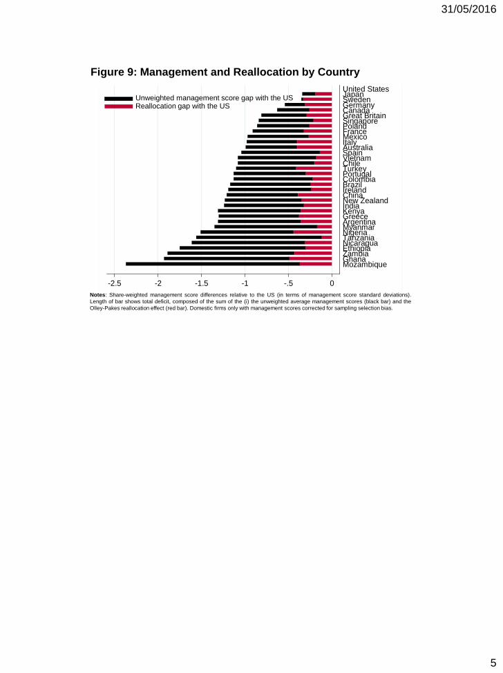
31/05/2016

5

-2.5 -2 -1.5 -1 -.5 0

United StatesJapanSwedenGermanyCanadaGreat BritainSingaporePolandFranceMexicoItalyAustraliaSpainVietnamChileTurkeyPortugalColombiaBrazilIrelandChinaNew ZealandIndiaKenyaGreeceArgentinaMyanmarNigeriaTanzaniaNicaraguaEthiopiaZambiaGhanaMozambique

Figure 9: Management and Reallocation by Country

Notes: Share-weighted management score differences relative to the US (in terms of management score standard deviations).

Length of bar shows total deficit, composed of the sum of the (i) the unweighted average management scores (black bar) and the

Olley-Pakes reallocation effect (red bar). Domestic firms only with management scores corrected for sampling selection bias.

Reallocation gap with the USUnweighted management score gap with the US

34

TABLE 1: CALIBRATED PARAMETERS FROM THE LITERATURE

Parameter Symbol value Rationale

Capital – output elasticity a 0.3 NIPA factor share

Labor – output elasticity b 0.6 NIPA factor share

Management – output elasticity c 0.1 Bloom et al (2013)

Demand elasticity ρ 5 Bartelsman et al (2013)

AR(1) parameter on ln(TFP) ρA 0.885 Cooper and Haltiwanger(2006)

Standard deviation of ln(TFP) σA 0.453 Cooper and Haltiwanger(2006)*

Discount Factor β 1/1.1 Standard 10% interest rate

Capital depreciation rate δK 10% Standard accounting assumption

Capital resale loss ϕK 50% Ramey and Shapiro (2001)

Notes: Fixed cost of production is normalized to 100 and mean of ln(TFP) is normalized to 1.

* Assumes measurement error on measured TFP has the same variance as true TFP as estimated in Bloom et al (2013).

35

TABLE 2: ESTIMATED PARAMETERS USING SIMULATED METHOD OF MOMENTS

PANEL A: PARAMETER ESTIMATES FROM SMM

Parameter Symbol Value

Depreciation rate of management δM 0.133 (0.055)

Adjustment cost parameter for management γM 0.207 (0.065)

Adjustment cost parameter for capital γK 0.189 (0.042)

Sunk cost of entry Κ 165.9 (6.78)

PANEL B: MOMENTS USED IN SMM ESTIMATES

Parameter Simulated Value Data Value

Standard deviation of 5 year management growth 0.559 0.564

Standard deviation of 5 year sales growth 0.936 0.948

Standard deviation of 5 year capital growth 0.883 0.875

Annual Exit rate 3.88% 3.89%

Notes: These are the parameters we estimate using the model (see text). Calibrated parameters from Table 1. Estimation by SMM on the management- accounting panel dataset of

up to 4907 firms. Standard errors generated by moment block-bootstrap and moment derivatives taken around the estimated parameter values.

36

TABLE 3: PERFORMANCE REGRESSIONS

(1) (2) (3) (4) (5) (6) (7) (8) (9) (10)

Dependent

variable Ln

(Sales)

Ln

(Sales)

Ln

(Sales)

Ln

(Sales)

Ln

(Sales)

Ln

(Employees)

Profitability

(ROCE, %)

5 year Sales

growth

Ln(Tobin

Q)

Death

(%)

Specification OLS OLS OLS OLS Olley-Pakes OLS OLS OLS OLS Probit

Management 0.356*** 0.159*** 0.154*** 0.035*** 0.231*** 0.402*** 1.005*** 0.043*** 0.030** -0.090**

(z-score) (0.018) (0.016) (0.019) (0.012) (0.031) (0.013) (0.296) (0.012) (0.015) (0.041)

Ln(Employees) 0.873*** 0.623*** 0.623*** 0.427*** 0.524***

(0.019) (0.024) (0.028) (0.060) (0.025)

Ln(Capital) 0.306*** 0.295*** 0.186*** 0.386***

(0.019) (0.022) (0.042) (0.098)

General

controls No Yes Yes Yes Yes Yes Yes Yes Yes Yes

Firm FE No No No Yes No No No No No No

Observations 12,146 10,900 8,877 8,877 6,433 24,501 12,578 11,291 6,572 7,507

Notes: *** denotes significance at the 1% level, ** denotes 5% significance and * denotes 10% significance. All columns estimated by OLS (except columns (5) and (10)) with standard errors in

parentheses under coefficients and clustered by firm. Column (5) uses the Olley-Pakes estimator. Column (10) uses probit estimation. Columns (1) to (9) are run on the combined full management-

accounting dataset panel from 2004 to 2014. Column (10) is run on the 2011 cross-section using firms surveyed up until 2010, with this cut-off defined to provide 4 years to measure exit (firms can

take up to 4 years to show up as dead in accounting data). Columns (3) and (4) restrict to firms which were surveyed in at least two different years. Column (5) restricts to firms with lagged capital

to generate investment data (the proxy variable in Olley-Pakes). “Management” is the firm’s normalized z-score of management (the z-score of the average z-scores of the 18 management questions).

“Profitability” is “Return on Capital Employed” (ROCE) and “5 year Sales growth” is the 5-year growth of sales defined as the difference of current and 5-year lagged logged sales. All columns

include a full set of country, three digit industry and time dummies. “Death” is the probability of exit by 2011 (sample mean is 2.4%). “Tobin’s Q” is the stock-market equity and book value of

debt value of the firm normalized by the book value of the firm, available for the publicly listed firms only. “General controls” comprises of firm age and the proportion of employees with college

degrees (from the survey), plus a set of survey noise controls which are interviewer dummies, the seniority and tenure of the manager who responded, the duration of the interviews and an indicator

of the reliability of the information as coded by the interviewer.

37

TABLE 4: COMPETITION AND MANAGEMENT

(1) (2) (3) (4) (5) (6)

Dependent Variable: Management (z-scored)

(1-Lerner) 0.990*** 1.751***

(0.366) (0.443)

Import Penetration 0.398** 0.830**

(0.170) (0.327)

Import Penetration – from China only 2.090** 2.204*

(0.972) (1.137)

Observations 8,630 8,630 8,630 8,630 8,630 8,630

Size- weight the regressions? No Yes No Yes No Yes

Notes: ** indicates significance at 5% level and * at the 10%. The dependent variable in all columns is the z-score of the average z-scores of the 18 management

questions. OLS estimates with standard errors in parentheses below coefficients. Standard errors are clustered at the industry by country by period cell in all

columns. “Lerner” is the median gross price-cost margin across all firms (from the ORBIS population) in the firm’s three digit SIC industry by country by

period cell; “Import penetration” is the value of all imports divided by apparent consumption (total production + imports - exports) in the plant’s ISIC Rev3

industry by country by period cell. “Import penetration – from China only” is the value of all imports originating from China divided by apparent consumption

in the plant’s ISIC Rev3 industry by country by period cell. All columns include only firms located in OECD countries and include all data collected across

2004-2014 survey waves. Industry is defined at the 3 digit SIC level in columns (1)-(2), and at the ISIC Rev3 level in columns (3)-(6). All columns include

ln(firm employment) and ln(plant employment), plus a full set of country by industry dummies and general controls (firm age and the proportion of employees

with college degrees (from the survey), a set of survey noise controls which are interviewer dummies, the seniority and tenure of the manager who responded,

the duration of the interviews and an indicator of the reliability of the information as coded by the interviewer). Columns (1) and (2) include a variable measuring

the log of the number of firms used to build the Lerner index in the country-industry-period cell. Columns (3)-(6) include the variable measuring apparent

consumption in the country-industry-period cell (the denominator of the import penetration variable) in levels. Employment weights are defined with respect to

total employment in the industry (3 digit SIC) by country cell.

38

TABLE 5: REALLOCATION TOWARDS BETTER MANAGED FIRMS

(1) (2) (3) (4) (5) (6)

Dep. Variable: Employees Employees Employees Employees Employees Employees

Management (M) 182.6*** 268.4*** 294.83*** 285.09*** 463.23*** 289.397***

(US is the omitted base) (20.8) (40.1) (77.22) (45.53) (105.09) (71.538)

Management*Employment -56.73* -59.21*

Protection (country level) (30.46) (30.66)

Management *Trade costs -0.10*** -0.16***

(country level) (0.03) (0.05)

Management *Tariff Levels -45.141*

(country*industry) (24.653)

MNG*Africa -144.6***

(52.1)

MNG*Americas -96.3**

(43.9)

MNG*(Other EU) -46.6

(58.5)

MNG*(South EU) -199.5***

(46.1)

MNG*Asia -64.3

(52.3)

Observations 8,991 8,991

7,272 8,918 7,272 8,087

Notes: *** indicates significance at the 1%, 5% (**) or 10% (*) level. Management*US is the omitted base in columns (1) and (2). Estimation by OLS with

standard errors clustered by firm. All columns include year, country, three SIC digit industry dummies, and general controls (firm age and the proportion of

employees with college degrees (from the survey), plus a set of survey noise controls which are interviewer dummies, the seniority and tenure of the manager who

responded, the duration of the interviews and an indicator of the reliability of the information as coded by the interviewer). The sample is domestic firms only (i.e.

no foreign or domestic multinationals). “M” is z-score of the average z-scores of the 18 management questions. “Sales growth” is one year ahead logarithmic

change. “Employment Protection” is the “Difficulty of Hiring” index is from World Bank (from 1 to 100). “Trade Cost” is World Bank measure of the costs to

export in the country (in US$). Tariffs are specific to the industry and country (MFN rates) kindly supplied by John Romalis (see Feenstra and Romalis, 2012).

39

TABLE 6: MANAGEMENT BY DESIGN - STYLES DIFFER DEPENDING ON ENVIRONMENT

(1) (2) (3) (4) (5) (6) (7) (8) (9)

People

Management

Monitoring

& Targets

Relative

People

People

Management

Monitoring

&Targets

Relative

People

People

Management

Monitoring

&Targets

Relative

People

(P) (MT) (P-MT) (P) (MT) (P-MT) (P) (MT) (P-MT)

Panel A: Using US Four digit industry (NBER, NSF)

ln(K/L) 0.018 0.107*** -0.118*** -0.000 0.096*** -0.125***

(0.015) (0.016) (0.018) (0.014) (0.016) (0.019)

R&D Intensity 0.136** 0.041 0.114 0.031 -0.125* 0.201***

(0.064) (0.087) (0.089) (0.062) (0.072) (0.074)

ln(%degree) 0.139*** 0.123*** 0.011

(0.008) (0.007) (0.010)

Observations 13,681 13,681 13,681 13,681 13,681 13,681 13,681 13,681 13,681

Panel B: Two-Digit industry by county specific value (KLEMS, OECD)

ln(K/L) -0.044 0.039 -0.104** -0.062 0.038 -0.126***

(0.040) (0.032) (0.040) (0.040) (0.034) (0.037)

R&D Intensity 0.496 0.100 0.476* 0.584 -0.004 0.721**

(0.358) (0.260) (0.249) (0.413) (0.254) (0.306)

ln(%degree) 0.132*** 0.071*** 0.070***

(0.015) (0.012) (0.019)

Observations 4,855 4,855 4,855 4,855 4,855 4,855 4,855 4,855 4,855

Notes: *** denotes 1% significant, ** denotes 5% significance and * denotes 10% significance. All dependent variables are z-scores of average z-scores of the underlying

questions. “People management” is the index built using all management questions between 13 to 18 and “Monitoring and targets” are all the remaining questions. All

columns estimated by OLS with standard errors in parentheses under coefficients. All columns control for two-digit SIC industry dummies, country and year dummies, ln(firm

employment) and ln(plant employment), plus a full set of general controls (firm age and the proportion of employees with college degrees (from the survey), plus a set of survey

noise controls which are interviewer dummies, the seniority and tenure of the manager who responded, the duration of the interviews and an indicator of the reliability of the

information as coded by the interviewer). In Panel A the capital-labor ratio is taken from the NBER Bartelsman-Grey dataset and R&D intensity is business R&D divided by

employment from NSF. Both capital-labor and R&D intensity are at the four digit level for the US and used across all countries (so no country-specific variation). In Panel B

the capital-labor ratio is measured at the two digit by country level from the EU KLEMs dataset and R&D/Value added is from the OECD STAN/ANBERD. EU-KLEMS is

only available for a restricted set of countries (Australia, Germany, Italy, Japan, Sweden, UK and US) hence the smaller sample size. Standard errors are clustered at the four

digit level in Panel A and two-digit industry by country level in Panel B.

40

TABLE 7: DECOMPOSITION OF CROSS COUNTRY TFP AND MANAGEMENT

(1) (2) (3) (4) (5) (6) (7)

country

Weighted

Manage

ment

Un-

weighted

Manage

ment

Covar-

iance

Mng.

Gap vs.

US

%

Reallo-

cation

TFP Gap

with US

% TFP

due

to Man-

agement

US 0.90 0.40 0.50 0 0

Japan 0.57 0.26 0.31 -0.33 56.64 -0.34 9.71

Sweden 0.55 0.38 0.17 -0.35 93.39 -0.08 43.49

Germany 0.36 0.18 0.19 -0.54 57.91 -0.19 28.72

Canada 0.27 0.04 0.24 -0.63 41.92 -0.13 48.64

UK 0.10 -0.11 0.21 -0.81 35.88 -0.15 55.34

Singapore 0.07 -0.23 0.29 -0.84 24.69

Poland 0.04 -0.20 0.23 -0.86 30.69 -0.22 39.26

France -0.01 -0.19 0.18 -0.91 35.29 -0.17 52.52

Mexico -0.07 -0.30 0.23 -0.97 28.21 -0.32 30.20

Australia -0.08 -0.18 0.10 -0.98 40.24 -0.19 51.56

Italy -0.08 -0.18 0.10 -0.98 41.05 -0.20 48.90

Spain -0.14 -0.50 0.36 -1.04 13.19 -0.27 39.03

Vietnam -0.18 -0.50 0.32 -1.08 16.42

Chile -0.19 -0.48 0.29 -1.09 18.81 -0.37 29.48

Turkey -0.20 -0.29 0.09 -1.10 36.92

Portugal -0.22 -0.43 0.20 -1.13 26.27 -0.41 27.41

Colombia -0.23 -0.51 0.28 -1.13 19.28 -0.66 17.21

Brazil -0.26 -0.51 0.25 -1.16 21.20 -0.79 14.63

Ireland -0.29 -0.55 0.26 -1.19 20.33

China -0.31 -0.41 0.11 -1.21 32.49 -0.90 13.44

NZ -0.33 -0.48 0.15 -1.23 28.44 -0.24 51.00

India -0.34 -0.52 0.17 -1.25 26.07 -0.73 17.20

Greece -0.40 -0.52 0.12 -1.30 29.09 -0.35 37.48

Kenya -0.40 -0.55 0.14 -1.30 27.26 -1.39 9.32

Argentina -0.41 -0.55 0.14 -1.31 27.74 -0.38 34.84

Myanmar -0.45 -0.78 0.33 -1.35 12.58

Nigeria -0.61 -0.67 0.06 -1.51 28.85

Tanzania -0.67 -1.04 0.37 -1.57 7.96 -1.34 11.74

Nicaragua -0.71 -0.89 0.19 -1.61 19.44

Ethiopia -0.85 -1.05 0.20 -1.75 17.09

Zambia -0.99 -1.05 0.06 -1.89 23.00 -3.04 6.22

Ghana -1.03 -1.04 0.01 -1.94 25.49 -2.00 9.69

Mzmbique -1.46 -1.60 0.13 -2.36 15.47 -1.10 21.40

Average -1.14 29.68 29.94

Notes: Colum (1) is employment share weighted management z-score. Column (2) is the unweighted score and Column (3) is

the management-employment covariance. Column (4) is the weighted management score in column (1) relative to US . Column

(5) is the proportion of relative weighted management score in column (1) due to reallocation. The country’s TFP relative to

the US in column (6) is from Penn World Tables version 8.1. (Feenstra et al, 2015) available at

http://www.rug.nl/research/ggdc/data/pwt/v81/the_next_generation_of_the_penn_world_table.pdf. Column (6) is the fraction

of the TFP gap with the US in column (6) that is due to the weighted relative management score in column (1). We assume a

one standard deviation increase in the management score causes a 10% increase in TFP (using Table 3 and Bloom et al, 2013).

All scores are adjusted for nonrandom selection into the management survey (see text). Only domestic firms used in these

calculations (i.e. multinationals and their subsidiaries are dropped).

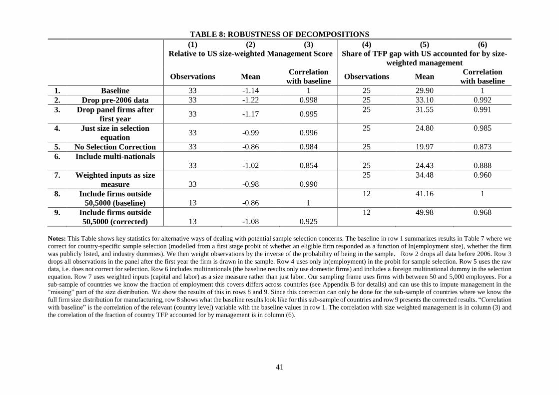
41

TABLE 8: ROBUSTNESS OF DECOMPOSITIONS

(1) (2) (3) (4) (5) (6)

Relative to US size-weighted Management Score Share of TFP gap with US accounted for by size-

weighted management

Observations Mean Correlation

with baseline Observations Mean

Correlation

with baseline

1. Baseline 33 -1.14 1 25 29.90 1

2. Drop pre-2006 data 33 -1.22 0.998 25 33.10 0.992

3. Drop panel firms after

first year 33 -1.17 0.995

25 31.55 0.991

4. Just size in selection

equation 33 -0.99 0.996

25 24.80 0.985

5. No Selection Correction 33 -0.86 0.984 25 19.97 0.873

6. Include multi-nationals

33 -1.02 0.854 25 24.43 0.888

7. Weighted inputs as size

measure 33 -0.98 0.990

25 34.48 0.960

8. Include firms outside

50,5000 (baseline) 13 -0.86 1

12 41.16 1

9. Include firms outside

50,5000 (corrected) 13 -1.08 0.925

12 49.98 0.968

Notes: This Table shows key statistics for alternative ways of dealing with potential sample selection concerns. The baseline in row 1 summarizes results in Table 7 where we

correct for country-specific sample selection (modelled from a first stage probit of whether an eligible firm responded as a function of ln(employment size), whether the firm

was publicly listed, and industry dummies). We then weight observations by the inverse of the probability of being in the sample. Row 2 drops all data before 2006. Row 3

drops all observations in the panel after the first year the firm is drawn in the sample. Row 4 uses only ln(employment) in the probit for sample selection. Row 5 uses the raw

data, i.e. does not correct for selection. Row 6 includes multinationals (the baseline results only use domestic firms) and includes a foreign multinational dummy in the selection

equation. Row 7 uses weighted inputs (capital and labor) as a size measure rather than just labor. Our sampling frame uses firms with between 50 and 5,000 employees. For a

sub-sample of countries we know the fraction of employment this covers differs across countries (see Appendix B for details) and can use this to impute management in the

“missing” part of the size distribution. We show the results of this in rows 8 and 9. Since this correction can only be done for the sub-sample of countries where we know the

full firm size distribution for manufacturing, row 8 shows what the baseline results look like for this sub-sample of countries and row 9 presents the corrected results. “Correlation

with baseline” is the correlation of the relevant (country level) variable with the baseline values in row 1. The correlation with size weighted management is in column (3) and

the correlation of the fraction of country TFP accounted for by management is in column (6).