What Drives Differences in Management?

by

Nicholas Bloom Stanford and NBER

Erik Brynjolfsson MIT and NBER

Lucia Foster U.S. Census Bureau

Ron Jarmin U.S. Census Bureau

Megha Patnaik Stanford

Itay Saporta-Eksten Tel-Aviv and UCL

John Van Reenen MIT, CEP and NBER

CES 17-32 March, 2017

The research program of the Center for Economic Studies (CES) produces a wide range of economic analyses to improve the statistical programs of the U.S. Census Bureau. Many of these analyses take the form of CES research papers. The papers have not undergone the review accorded Census Bureau publications and no endorsement should be inferred. Any opinions and conclusions expressed herein are those of the author(s) and do not necessarily represent the views of the U.S. Census Bureau. All results have been reviewed to ensure that no confidential information is disclosed. Republication in whole or part must be cleared with the authors. To obtain information about the series, see www.census.gov/ces or contact J. David Brown, Editor, Discussion Papers, U.S. Census Bureau, Center for Economic Studies 5K034A, 4600 Silver Hill Road, Washington, DC 20233, CES.Working.Papers@census.gov. To subscribe to the series, please click here.

Abstract

Partnering with the Census we implement a new survey of “structured” management practices in 32,000 US manufacturing plants. We find an enormous dispersion of management practices across plants, with 40% of this variation across plants within the same firm. This management variation accounts for about a fifth of the spread of productivity, a similar fraction as that accounted for by R&D and twice as much as explained by IT. We find evidence for four “drivers” of management: competition, business environment, learning spillovers and human capital. Collectively, these drivers account for about a third of the dispersion of structured management practices. Keyword: Management, productivity, competition, learning JEL Classification: L2, M2, O32, O33 *

* Any opinions and conclusions expressed herein are those of the authors and do not necessarily represent the views of the U.S. Census Bureau. All results have been reviewed to ensure that no confidential information was disclosed. Financial support was provided in part by the National Science Foundation, Kauffman Foundation and the Sloan Foundation and administered by the National Bureau of Economic Research. In addition, Bloom thanks, the Toulouse Network for Information Technology, Brynjolfsson thanks, the MIT Initiative on the Digital Economy and Van Reenen thanks, the European Research Council and Economic and Social Research Council for financial support. We thank Hyunseob Kim for sharing data on large plant openings. We are indebted to numerous Census Bureau staff for their help in developing, conducting and analyzing the survey; we especially thank Julius Smith, Cathy Buffington, Scott Ohlmacher and William Wisniewski. This paper is an updated version of a working paper previously titled “Management in America” and we thank our formal discussant Andrea Pratt as well as numerous participants at seminars for many helpful comments.

2

1 Introduction

The interest of economists in management goes at least as far back as On the Sources of Business

Profits by Francis Walker (1887), the founder of the American Economic Association and the

Superintendent of the 1870 and 1880 Censuses.1 This interest has persisted until today. For

example, Syverson’s (2011) survey of productivity devotes a section to management as a potential

driver, noting that “no driver of productivity has seen a higher ratio of speculation to research.”

Work evaluating differences in management is often limited to relatively small samples of plants

(e.g., Ichniowski, Shaw and Prenushi, 1997; Bresnahan, Brynjolfsson and Hitt, 2002), developing

countries (e.g., Bloom, Eifert, Mahajan, McKenzie and Roberts, 2013, and Bruhn, Karlan and

Schoar, 2016) or particular historical episodes (e.g., Giorcelli, 2016). In addition, although

previous work on larger samples such as Bloom, Sadun and Van Reenen (2016) has measured

differences in management across firms and countries, there is no large-scale work on the

variations in management between the plants2 within a firm.

There are compelling theoretical reasons to expect that management matters for

performance. Gibbons and Henderson (2013) argue that management practices are a key reason

for persistent performance differences across firms due to relational contracts. Brynjolfsson and

Milgrom (2013) emphasize the role of complementarities among management and organizational

practices. Halac and Prat (2016) show that “engagement traps” can lead to heterogeneity in the

adoption of practices even when firms are ex ante identical. This paper provides empirical

evidence for the role that management practices play in firm and plant performance by examining

the first large sample of plants with this information.

We partnered with the Economic Program Directorate of the U.S. Census Bureau to

develop and conduct the Management and Organizational Practices Survey (MOPS).3 This is the

first-ever mandatory government management survey, covering more than 30,000 plants across

more than 10,000 firms.4 The size and high response rate of the dataset, its coverage of units within

1 Walker was also the second president of MIT and the vice president of the National Academy of Sciences.

Arguably Adam Smith’s discussion of the famous Pin Factory and the division of labor was an even earlier antecedent.

2 Because we are focusing on manufacturing, we use the words “plants” and “establishments” interchangeably. 3 This survey was only possible with the generous provision of over $1million of research support from our primary

donors - the National Science Foundation, the Kauffman Foundation and the Sloan Foundation. 4 See the descriptions of MOPS in Bloom, Brynjolfsson, Foster, Jarmin, Saporta-Eksten, and Van Reenen (2013)

and Buffington, Foster, Jarmin and Ohlmacher (2016).

3

a firm, its links to other Census data, as well as its comprehensive coverage of industries and

geographies makes it unique, and it enables us to address some of the major gaps in the recent

management literature.

We start by examining the variation in management practices across plants, showing three

key results. First, there is enormous inter-plant variation in management practices. Although 18%

of establishments adopt three-quarters or more of a package of basic structured management

practices for performance monitoring, targets and incentives, 27% of establishments adopt less

than half of such practices. Second, about 40% of the variation in management practices is across

plants within the same firm. That is, in multi-plant firms, there is considerable variation in practices

across units.5 The analogy for universities would be that variations in management practices across

departments within universities are almost equally large as the variations across universities.

Third, these variations in management practices are increasing in firm size. That is, larger firms

have substantially more variation in management practices. This appears to be largely explained

by the greater spread of larger firms across different geographies and industries.

We then turn to examining whether our management measures are linked to performance.

We find that plants using more structured management practices have greater productivity,

profitability, innovation (as proxied by R&D and patent intensity) and growth. This relationship is

robust to a wide range of controls including industry, education, plant and firm age, and possible

survey noise. The relationship between management and performance also holds over time within

plants (plants that adopted more of these practices between 2005 and 2010 saw improvements in

their performance between 2005 and 2010) and across establishments within firms at a point of

time (establishments within the same firm with more structured management practices achieve

better performance outcomes). These management practices also have a highly significant

predictive power for future growth and firm survival up to three years ahead (the current limit of

our data after the MOPS survey).

5 A literature beginning with Schmalensee (1985) has examined how the variance in profitability of business across

business divisions decomposes into effects due to company headquarters, industry and other factors. Several papers have examined productivity differences across sites within a single firm. For example, Chew, Bresnahan and Clark (1990) looked at 40 operating units in a commercial food division of a large US corporation (the top ranked unit had revenue based Total Factor Productivity twice as high as the bottom ranked). Argote et al. (1990) showed large differences across 16 Liberty shipyards in World War II. Freeman and Shaw (2009) contains several studies looking at performance differences across the plants of single multinational corporations.

4

The magnitude of this management-productivity relationship is large. Increasing structured

management from the 10th to 90th percentile can account for about 18% of the comparable 90-10

spread in firm total factor productivity (TFP).6 Using the same dataset, we also examine the

association of productivity with other common “drivers” and find that the 90-10 spread in R&D

accounts for about 17% of the spread in firm TFP, employee skills about 11%, and IT expenditure

per employee about 8%. Of course, all these magnitudes are dependent on a number of other

factors, such as the degree of measurement error in each variable, but they do highlight that

variation in management practices is likely a key factor accounting for variation in TFP. These

factors are also interrelated - when we examine them jointly, we find they account for about 33%

of the total variation in 90-10 productivity. Given estimates that about 50% of the variation in

productivity is measurement error (Collard-Wexler, 2013 and Bloom, Floetotto, Jaimovich,

Saporta and Terry, 2016), this suggests that these factors – management, innovation, IT and skills

– together account for about two-thirds of the real spread in firm productivity.

We next examine some “drivers” of management practices. We focus our analysis on four

potential candidates: product market competition, business environment, learning spillovers from

large manufacturing plant entry (primarily belonging to multinational corporations), and

education.

The selection of these four factors follows from the existing management and productivity

literature which is motivated by a number of different theoretical perspectives (e.g. Syverson, 2011

or Gibbons and Roberts, 2013). One perspective that binds our drivers together follows Walker

(1887) and considers some forms of structured management practices to be akin to a productivity-

enhancing technology. This naturally raises the question of why all plants do not immediately

adopt these practices. One factor is differential ability, which motivates our examination of human

capital. Another factor is information – not all firms are aware of the practices or believe that they

would be beneficial. This motivates our examination of diffusion-based learning and informational

spillovers from Million Dollar Plants. Finally, the degree to which the higher ability/better

informed establishments drive out their less productive counterparts will depend on the

environment. The selection of such plants will be weaker when the business environment is less

6 We use TFP as shorthand for revenue based Total Factor Productivity. This will contain an element of the mark-

up (see Hsieh and Klenow, 2009) but is likely to be correlated with quantity based TFP (see Bartelsman, Haltiwanger and Scarpetta, 2013).

5

competitive and/or more distorted by regulatory frictions - which motivates our analysis of

competition and regulation.

By using the plausibly exogenous variation within our dataset, we help to identify the

causal effects of these factors on the adoption of structured management practices.

For product market competition, we undertake two strategies. First, we calculate the

industry Lerner index and look at cross sectional and panel variation. Second, we exploit changes

in exchange rates that differentially affect the plant’s industry depending on which countries are

competing in its output market. We find that product market competition increases the adoption of

structured management practices, particularly at plants in the lower tail of the structured

management distribution.

On business environment, we exploit both the location of plants around the border between

“Right to Work” and non-“Right to Work” states and the location of firms’ oldest surviving plants

in multi-plant firms to identify impacts of business environment on management practices. We

find “Right to Work” rules, which are a proxy for the state business environment - including

reduced influence of labor unions as well as “pro-business” policies such as more flexible

environmental and safety regulations (see Holmes, 1998) - seem to increase structured

management practices around firing and promotions but seem to have little impact on other

practices.

To investigate learning spillovers, we build on Greenstone, Hornbeck and Moretti’s (2010)

identification strategy using “Million Dollar Plants” – large investments for which both a winning

county and a runner-up county are known. Comparing the counties that “won” the large, typically

multinational plant versus the county that narrowly “lost,” we find significant positive impacts on

management practices, TFP and employment. Importantly, the positive spillovers only arise if the

winning entrant was also a manufacturing plant, suggesting localized managerial spillovers tend

to be mainly within the same sector (recall that the MOPS data solely relates to manufacturing

plants).

Finally, to obtain causal impacts of education, we follow Moretti (2010) to use the quasi-

random location of land-grant colleges as an instrument for local supply of more educated labor.

We find large significant effects on management practices of being near a land-grant college with

a range of controls for other local variations in population density, income and other county-level

and firm-level controls.

6

Our estimates imply that these four drivers account for around a third of the 90-10 between-plant

spread of structured management practices. Although this is a non-trivial fraction, it leaves plenty

of room for other determinants of these management practices.

The paper is structured as follows. In Section 2, we describe the management survey; in

Section 3, we detail the variation of management practices across and between firms; and in

Section 4, we outline the relationship between management and performance; in Section 5, we

examine potential drivers of management practices. Finally, in Section 6 we conclude and

highlight areas for future analysis.

2 Management and Organizational Practices Survey

The Management and Organizational Practices Survey (MOPS) was jointly funded by the Census

Bureau and the National Science Foundation and was delivered as a mandatory supplement to the

Annual Survey of Manufacturers (ASM).7 The original design was based in part on a survey tool

used by the World Bank and adapted to the U.S. through several months of development and

cognitive testing by the Census Bureau.8 It was sent electronically as well as by mail to the ASM

respondent for each establishment,9 which was typically the plant manager or financial

comptroller. Most respondents (58.4%) completed the survey electronically, with the remainder

completing the survey by paper. Non-respondents were mailed a follow-up letter after six weeks

if no response had been received. A second follow-up letter was mailed if no response had been

received after 12 weeks. The first follow-up letter included a copy of the MOPS instrument. An

administrative error occurred when merging Internet and paper collection data that caused some

respondents to receive the first follow-up even though they had already responded. We exploit this

accident to deal with measurement error in the management scores in Section 3.

2.1 Measuring Management

The survey contained 16 management questions in three main sections: monitoring, targets and

7 For more details see Buffington, Foster, Jarmin and Ohlmacher (2016). 8 See Buffington, Herrell and Ohlmacher (2016) for more information on the testing and development of the MOPS. 9 The Appendix provides more details on datasets.

7

incentives, based on Bloom and Van Reenen (2007), which itself was based in part on the

principles of continuous monitoring, evaluation and improvement from Lean manufacturing (e.g.,

Womack, Jones and Roos, 1990). The survey also contains questions on other organizational

practices (such as decentralization) based on work by Bresnahan, Brynjolfsson and Hitt (2002) as

well as some background questions on the plant and the respondent.

The monitoring section asked firms about their collection and use of information to monitor

and improve the production process. For example, the survey asked, “How frequently were

performance indicators tracked at the establishment?”, with response options ranging from “never”

to “hourly or more frequently.” The targets section asked about the design, integration and realism

of production targets. For example, the survey asked, “What was the time-frame of production

targets?”, with answers ranging from “no production targets” to “combination of short-term and

long-term production targets.” Finally, the incentives section asked about non-managerial and

managerial bonus, promotion and reassignment/dismissal practices. For example, the survey

asked, “How were managers promoted at the establishment?”, with answers ranging from “mainly

on factors other than performance and ability, for example tenure or family connections” to “solely

on performance and ability.” 10

In our analysis, we aggregate the results from these 16 questions into a single measure of

“structured management.” This management score is the unweighted average of the score for each

of the 16 questions, where the responses to each question are first scored to be on a 0-1 scale. Thus,

the summary measure is scaled from 0 to 1, with 0 representing an establishment that selected the

category which received the lowest score (little structure around performance monitoring, targets

and incentives) on all 16 management dimensions and 1 representing an establishment that selected

the category that received the highest score (an explicit structured focus on performance

monitoring, detailed targets and strong performance incentives) on all 16 dimensions.

2.2 Sample and Sample Selection

Overall, 49,782 MOPS surveys were successfully delivered, and 37,177 responses were received,

yielding a response rate of 78%, which is similar to the response rate of the main ASM survey. For

10 The full questionnaire is available on http://www.census.gov/mcd/mops/how_the_data_are_collected/MP-

10002_16NOV10.pdf

8

most of our analysis, we further restrict the sample to establishments with at least 11 non-missing

responses to management questions that also have positive value added, positive employment and

positive imputed capital in the ASM. Table A1 shows how our various samples are derived from

the universe of establishments.11

Table A2 provides more descriptive statistics on the samples we use for analysis. The mean

establishment size is 167 employees and the median (fuzzed) is approximately 80. The average

establishment in our sample has been in operation for 22 years, 44% of managers and 9% of non-

managers have college degrees, 13% of workers are in unions, 42% of plants export, and 69% of

plants are part of larger multi-plant firms. Finally, Table A3 reports the results for linear probability

models for the different steps in the sampling process. We show that establishments that were

mailed and responded to the MOPS survey are somewhat larger and more productive compared to

those that did not respond, but these differences are quantitatively small.

2.3 Performance Measures

In addition to our management data, we also use data from other Census and non-Census data sets

to create our measures of performance (productivity, profitability, innovation, and growth). We

use establishment-level data on sales, value-added and labor inputs from the ASM to create

measures of growth and labor productivity. As described in detail in the Appendix, we also

combine capital stock data from the Census of Manufactures (CM) with investment data from the

ASM and apply the Perpetual Inventory Method to construct capital stock at the establishment

level, which we use to create measures of total factor productivity. For innovation, we use firm-

level data from the 2009 Business R&D and Innovation Survey (BRDIS) on R&D expenditure and

patent applications by the establishment’s parent firm (from the USPTO).

3 Management Practices across Plants and Firms

Figure 1 plots the histogram of plant management scores, which displays enormous dispersion.

11 Table A1 reports the results for linear probability models for the different steps in the sampling process. We show

that establishments that were mailed and responded to the MOPS survey are somewhat larger and more productive compared to those that did not respond, but these differences are quantitatively small.

9

While 18% of establishments have a management score of at least 0.75, meaning they adopt 75%

of the most structured management practices, 27% of establishments receive a score of less than

0.5 (that is, they adopt less than half the practices).

One important question is: to what extent do these variations in management practices

across plant occur within rather than between firms? The voluminous case-study literature on

management practices often highlights the importance of variations both within and between

organizations, but until now it has been impossible to measure these separately due to the lack of

large samples with both firm and plant variation. The benefit of the large MOPS sample is that we

have multiple plants per firm, making this the first opportunity to evaluate variations within and

between firms accurately.

Before decomposing the between-plant management dispersion into a within-firm

component and a between-firms component, we need to address a major challenge: the bias

induced by measurement error. Measurement error in plant-level management scores will inflate

the plant-level variation and thus bias downwards the component of the overall plant-level

variation we attribute to the firm-level component. Estimates in Bloom and Van Reenen (2007)

from independent repeat management surveys (at the same point of time) imply that measurement

error accounts for 25% of the variation in management score and 42% of the variation at the

practices level, making this an important issue.

To address this challenge, we exploit a valuable feature of the 2010 MOPS survey, which

is that approximately 500 plants from our baseline sample have two surveys filled out by different

respondents.12 That is, for this set of plants, two individuals – for example the plant manager and

plant comptroller – both independently filled out the MOPS survey.13 This is most likely because

a follow-up letter was mailed to the plant in error that included a form and online login information,

and an individual other than the original respondent received the letter. These double responses

provide very accurate gauges of survey measurement error, because within a narrow three-month

window we have two measures of the same plant-level management score provided by two

independent respondents. From correlation analysis of the two sets of completed surveys, we find

12 For disclosure avoidance reasons, we cannot provide exact sample sizes, but this data is available through the

Federal Statistical Research Data Centers. 13 In total, approximately 1,200 plants from the baseline sample completed the survey more than once, either once

on paper and once online or twice on paper. Of these, about 500 provided a second response filled out by a different respondent.

10

that measurement error accounts for 45.4% of the observed management variation across plants.14

This measurement also turns out to be independent of any firm- or plant-level observable

characteristic such as employment or the number of plants in the firm (see Appendix Table A4),

and thus appears to be effectively white noise.

Armed with this estimate of 45.4% of the variation accounted for by measurement error,

we can now decompose the remaining variation in the management score into the part accounted

for by the firm and the part accounted for by the plant. To do this, we keep the sample of 16,50015

out of 31,793 plants in the sample that are in multi-plant firms with two or more plants in the

MOPS survey. Although this sample only contains 44% of the overall sample, these are larger

plants and account for 74% of total output in the MOPS sample.

The first series in Figure 2 (blue diamonds) plots the share of the plant-level variation in

the management score accounted for by the parent firm in firms with 2 or more plants after scaling

by (0.546=1-0.454) to account for measurement error. To understand this graph, first note that the

top left point is for firms with exactly two plants. For this sample, firm fixed effects account for

90.4% of the adjusted R-squared in management variation across plants,16 with the other 9.6%

accounted for by variation across plants within the same firm. So, in smaller two-plant firm

samples, most of the variation in management practices is due to differences across firms.

Moving along the x-axis in Figure 2, we see that the share of management variation

attributable to the parent firm declines as firm size rises. For example, in firms with 50-74 plants,

the parent firm accounts for about 40% of the observed management variation, and in firms with

150 or more plants, the parent firm accounts for about 35% of the variation. Hence, in samples of

plants from larger firms, there is relatively more within-firm variation and relatively less cross-

firm variation in management practices.

At least two important results arise from Figure 2. First, both plant-level and firm-level

14 Assuming the two responses have independent measurement error with standard deviation M, and defining T as

the true management standard deviation, the correlation between the two surveys will be T/(T+M). Interestingly, this 45.4% share of the variation from measurement error is very similar to the 49% value obtained in the World Management Survey from second independent telephone interviews (Bloom and Van Reenen, 2010).

15 Note that because of clearance restrictions, many sample sizes have been rounded. 16 It is essential for this part of the analysis that the adjusted R2 on the firm fixed effects is not mechanically decreasing

in the number of establishments in the firm. To alleviate any such concern, we simulated management scores for establishments linked to firms with the same sample characteristics as our real sample (in terms of number of firms and number of establishments in a firm), but assuming no firm fixed effects. We then verified – shown in Appendix Figure A1 – that indeed for this sample, the adjusted R2 is zero and does not show any pattern over the number of establishments in a firm.

11

factors are important for explaining differences in management practices across plants, with the

average share of management variation accounted for by firms being 58% (so 42% is across plants

within the same firm). Second, the share of management practice variation accounted for by the

parent firm is declining in the overall size of the firm, as measured by the number of

establishments.

What explains the large fraction of within-firm variation in management practices? One

likely explanation is that within a firm, different establishments operate in different environments

– for example, different industries or locations, in which different management practices are

appropriate. To evaluate this explanation, the second series in Figure 2 (green dots) repeats the

analysis with one change: when we run the regressions of management on firm fixed effects (used

to recover the adjusted R2), we control for the part of the management score that is explained by

within firm/across plant industry and MSA variation.17 This essentially removes the within-firm

share of variation in management that is explained by industry and geographical variation. There

are two points to highlight from this exercise. First, by construction, the overall within-firm

management variation is smaller, going down from 42% on average to 19%. Second, the relation

between size and within-firm variation is flatter, where we cannot reject the null that the within-

firm variation is similar for 10 and 150+ plants firms. This is consistent with larger firms (those

with more than 10 employees) operating across more industries and geographical regions, which

accounts for their greater within firm spread in management practices.

We further explore these points in Table 1, reporting results from a regression of the within-

firm standard deviation of the management score on firm level characteristics.18 Consistent with

first series in Figure 2 (blue diamonds), columns (1) and (2) demonstrate that the standard deviation

of management within a firm is increasing with the number of establishments in the firm, and that

this relation is stronger for firms with 10 establishments or less. Column (3) shows that operating

in more industries and over more locations are both correlated with a larger within-firm spread of

management. Columns (4) and (5) are consistent with the results in the second series in Figure 2

17 Specifically, the R2 regressions include now the linear projection of management from a regression of management

on full sets of NAICS and MSA dummies (where for plants in areas without an MSA, the state is used), where the regression also includes firm fixed effects. The sample for this regression is identical in both series in Figure 2.

18 Our management score is bounded between 0 and 1. To ensure our regressions are not exposed to a mechanical relation whereby better-managed firms show smaller standard deviation of management because their establishments are pushed towards the upper bound of the score, we control in all regressions for a 5 degree polynomial of average management at the firm (results are almost identical for 3, 4, 6, or 7 degree polynomial).

12

(green dots): once controlling for the number of within-firm industries and locations, the relation

between management spread and size weakens and becomes insignificant for firms with more than

10 manufacturing establishments. Columns (6)-(11) show that the within-firm spread of

management is correlated with other factors in an intuitive way. Although we do not find a

correlation between the spread of management and the spread of establishment age within the firm

(column (6)), we find that the spread of management is larger for firms with a larger employment

spread (column (7)).19 We also find a larger spread for firms with more ownership changes over

the past one, two and three years (columns (8) to (10)), suggesting it takes at least three years after

a firm acquires a new plant to change its management practices.20

4 Management and Performance

Given the variations in management practices noted above, an immediate question is whether these

practices link to performance outcomes. In this section, we investigate whether these more

structured management practices are correlated with five measures of performance (productivity,

growth, survival, profitability, and innovation). Although there is good reason to think

management practices affect performance, we do not necessarily attribute a causal interpretation

to the results in the section. Instead, it suffices to think about these results as a way to establish

whether this management survey is systematically capturing meaningful content rather than just

statistical noise.

4.1 Management and Productivity

We start by looking at the relation between labor productivity and management. Suppose that the

establishment production function is:

(1)

where Yit is real value added (output - materials), Ait is productivity (excluding management

19 Interestingly, in the MOPS survey, we also asked about the extent of decentralization of plant-level decisions over

hiring, investment, new products, pricing and marketing and found this was also significantly higher in larger firms (see Aghion et al., 2015).

20 We have also checked for the correlation with 4- and 5-year ownership changes, finding decreasing point estimates with no statistical significance.

13

practices), Kit denotes the establishment's capital stock at the beginning of the period, Lit are labor

inputs, Xit is a vector of additional factors such as education, and Mit is our management score.21

Management is an inherently multi-dimensional concept, so for this study we focus on a single

dimension: the extent to which firms adopt more structured practices.22

Dividing by labor and taking logs we can rewrite this in a form to estimate on the data

log 1 log (2)

where we have substituted the productivity term (Ait) for a set of industry (or establishment or

firm) fixed effects and a stochastic residual eit. Because we may have multiple establishments

per firm, we also cluster our standard errors at the firm (rather than establishment) level.

In Table 2 column (1), we start by running a basic regression of labor productivity

(measured as log(value added/employee)) on our management score without any controls. We find

a highly significant coefficient of 1.272, suggesting that every 10% increase in our management

score is associated with a 13.6% (13.6% = exp(0.1272)) increase in labor productivity. To get a

sense of this magnitude, our management score has a sample mean of 0.64 and a standard deviation

of 0.152 (see the sample statistics in Appendix Table A2), so that a one standard-deviation change

in management is associated with a 21.3% (21.3% = exp(0.152*1.272)) higher level of labor

productivity (see also Table 3). We provide more detailed magnitudes analysis in sub-section 4.3.

In column (2) of Table 2, we estimate the full specification from equation (1) with capital

intensity, establishment size and employee education, industry dummies and “noise controls” (for

potential survey bias such as whether the form was filled out online or offline). This reduces the

coefficient on management to about 0.5. Even after conditioning on many observables, a key

question that remains is whether our estimated OLS management coefficient captures a relation

between management and productivity, or whether it is just correlated with omitted factors that

affect the management score and the productivity measure.

Using the 2005 recall questions, matched to the 2005 ASM files, we can construct a two

period panel of management, productivity and other controls, to at least partially address this

21 We put the management score and Xit controls to the exponential simply so that after taking logs we can include

them in levels rather than logs. 22 The individual practices are highly correlated, which may reflect a common underlying driver or

complementarities among the practices (see e.g., Brynjolfsson and Milgrom, 2013). In this exercise, we use the mean of the share of practices adopted, but other measures like the principal factor component or z-score yield extremely similar results.

14

concern over omitted factors. As long as the unobserved factors that are correlated with

management are fixed over time at the establishment level (corresponding to in equation (1)),

we can difference them out by running a fixed effect panel regression. Column (3) reports the

results for the 2005-2010 pooled panel regression (including a 2010 time dummy).23 The

coefficient on management, 0.298, remains significant at the 1% level. Of course, this coefficient

may still be upwardly biased if management practices are proxies for time-varying unobserved

shocks. On the other hand, the coefficient on management could also be attenuated towards zero

by measurement error, and this downward bias is likely to become much worse in the fixed-effect

specification.24

The rich structure of our data also allows us to compare firm-level versus establishment-

level management practices. In particular, by restricting our analysis to multi-establishment firms,

we can check whether there is a correlation between structured management and labor productivity

within a firm. When including a firm fixed effect in the cross section of plants, the coefficient on

management is identified solely off the variation of management and productivity across plants

within each firm in 2010. Column (4) of Table 2 shows OLS estimates for the sub-sample of multi-

establishment firms with firm-effects. The within-firm management coefficient of 0.233 is highly

significant. Hence, even within the very same firm, when management practices differ across

establishments, we find large differences in productivity associated with these variations in

management practices. This is reassuring since we have shown that there is a large amount of

management variation across plants within the same firm.

So far, we have established a strong correlation between labor productivity and the

adoption of management practices. It is likely that this relation is somewhat contingent on the

firm’s environment, and that the adoption of particular management practices is more important

in some contexts than in others. To investigate this heterogeneity, we estimate the specification in

column (2) of Table 2 for the 86 four-digit manufacturing NAICS categories. Figure 3 plots the

smoothed histogram of the 86 regression coefficients.25 The distribution is centered on 0.5, which

23 Note that the sample is smaller, because we now require non-missing controls also for 2005. In particular, we have

to drop plants that entered after 2005, and plants that were not part of the previous ASM rotating panel (the panel is revised every 5 years, at years ending 4 and 9).

24 There is certainly evidence of this from the coefficient on capital, which falls dramatically when establishment fixed effects are added, which is a common result in the literature.

25 To comply with Census disclosure avoidance requirements, we do not report the actual coefficients industry by industry, but a smoothed histogram.

15

reassuringly is the coefficient from the pooled regression. Ninety-two percent of establishments

operate in industries with a positive labor productivity-management relation.

Nevertheless, Figure 3 demonstrates that indeed there is a lot of heterogeneity, and an F-test

for the null of no difference across industries is easily rejected (p-value<0.001). These findings

suggest that structured management is differentially important across environments as one would

expect. We leave a more thorough investigation of the reasons for this heterogeneity for future

research, but we did examine whether structured management was less important for productivity

in sectors where innovation mattered a lot (e.g. high industry intensities of R&D and/or patenting),

as perhaps an over-focus on productive efficiency could dull creativity. Perhaps surprisingly, we

found that the productivity-management was actually stronger in these high tech industries,

perhaps implying that rigorous management of R&D labs is as important as production plants.

4.2 Management and Other Performance Measures (Growth, Profitability

and Innovation)

In column (5) of Table 2, we examine another performance measure: employment growth between

2010 (the year of the MOPS data) and 2013 (the last year of the ASM panel). Establishments with

more structured management practices grew significantly faster in future years.26 Column (6) adds

the 2010 level of TFP27 to the right-hand side of the employment growth equation and not

surprisingly finds that this also has predictive power for future employment growth. Interestingly,

adding TFP does not substantially diminish the coefficient on management, suggesting that both

TFP and management provide predictive power for future employment growth. Moreover, we also

see that the t-statistic on management (about 10) is more than double the t-statistic on TFP (about

4), which highlights how informative the management score is for plant performance.

Columns (7) and (8) of Table 2 perform a similar analysis for a plant’s exit probability

between 2010 and 2013, and we again find that the management score is highly predictive of future

performance. In terms of magnitudes, the unconditional probability of exit between 2010 and 2013

is 7% in our sample, and a one standard deviation increase in management is associated with a 2

percentage point decline in this exit probability (i.e., a 29% drop in the exit rate). For comparison,

26 To make interpretation and comparison between management score and TFP easier, both management and TFP are

normalized by their standard deviation in columns (5)-(8). 27 This is constructed following the standard approach in Foster, Haltiwanger and Krizan (2001) – see Appendix A.

16

a one standard deviation increase in TFP is associated with a 0.8 percentage point decline in exit

probability (an 11% drop in the exit rate). Column (9) looks at profitability (operating profits

divided by sales), and finds that establishments with higher management scores are significantly

more profitable. Finally, Column (10) looks at a classic measure of innovation – R&D spending

per employee – and finds a strongly positive significant correlation with management for a sample

of MOPS plants that match the Business R&D and Innovation Survey.28

We also ran a series of other robustness tests on Table 2, such as using standardized z-

scores (rather than the 0-1 management scores), dropping individual questions that might be

output-related and using ASM sampling weights, and we found very similar results.

A non-parametric description of these management and plant performance correlations is

shown in Figure 4. This confirms the robust positive and broadly monotonic relationship between

structured management and productivity, profitability, growth, exporting, R&D and patenting

reported in the regression analysis.29 Figure A1 cuts the data in another way, plotting the size of

establishments and firms against their management scores, showing a continuous positive

relationship from sizes of 10 employees upwards. These panels show that both establishment and

firm management scores are rising in size until they reach about 5,000 employees, after which the

relationship levels off. This difference is also quantitatively large. A firm with 10 employees has

a management score of 0.5 compared to 0.7 for a firm with 1,000 employees. This is comparable

to moving from approximately the 20th percentile to the 70th percentile of the management score

distribution.

Finally, while most of our analysis in this section has focused on within-industry

management-performance relationships, a similar positive association between management and

firm performance is observed across industries and locations. Appendix Table A5 replicates

columns (5) and (7) of Table 2 examining performance, this time first collapsing the data by taking

means over the 471 NAICS industry codes (columns (1) and (2)), and then by collapsing the data

at the county level (columns (3) and (4)). The management-performance relation remains large

28 Running the same regression on another measure of innovation, log(1+patents), we find a similarly significant

coefficient (standard error) of 0.510 (0.101). 29 Under the Milgrom and Roberts (1990) model of complementarity organizational practices we might have expected

a more convex relationship, with large rises in performance only visible in plants that adopt a large number of complementary practices (e.g. Ichniowski et al, 1997; Meagher and Strachan, 2016). Our evidence suggests that such complementarities may be second order or that the data is too coarse to identify these effects.

17

and statistically significant – industries and regions with higher management scores have

significantly higher growth and rates of survival.30 This is an important point for motivating the

analysis conducted in Section 5, where industry and geography provide variation for the

identification of management drivers.

4.3 Magnitudes of the Management and Productivity Relationship

To get a better sense of the magnitudes of the management-productivity relation, we compare

management to other factors that are commonly considered important drivers of productivity:

R&D, information technology (IT) and human capital. We focus on these three because they are

leading factors in driving TFP differences (e.g., discussed in detail in the survey on the

determinants of productivity in Syverson, 2011), and because we can measure them well using the

same sample of firms used for the analysis of the management-productivity link. In particular, we

ask how much of the 90-10 TFP spread can be accounted for by the 90-10 spread of management,

R&D expenditure, IT investment per worker, and human capital (measured as the share of

employees with a college degree).

Columns (1)-(4) of Table 3 report the results from firm-level regressions of TFP on those

factors. To obtain an aggregate firm-level TFP measure, the dependent variable is calculated as

industry-demeaned TFP at the firm level, where the establishments within a firm are weighted by

total value of shipments.31 The bottom row of column (1) shows that the 90-10 spread in

management accounts for about 18% of the spread in TFP. In columns (2) to (4) we examine R&D,

IT and skills and find these measures account for 17%, 8% and 11% of the 90-10 TFP gap,

respectively. Column (5) shows that the role of management remains large in the presence of the

other factors, and that jointly these can account for about a third of the 90-10 spread in TFP. Given

estimates that about 50% of firm-level TFP is measurement error (see Collard-Wexler, 2013 and

Bloom et al., 2016),32 this indicates these four factors – management, innovation, IT and human

30 We focused on employee growth and survival, because they are more comparable across industries. Results also

were significant for other measures like value-added per employee, but these could be concerns over cross-industry and region variations arising due to technological and price level variations.

31 We run the regression at the firm level, because R&D is only measured at the firm level, making it easier to compare between factors. To obtain the firm-level measure, we weight the right-hand variables by their plant’s share of total shipments (exactly as we do for the dependent variable).

32 We make this calculation under the assumption that measurement error in TFP is not correlated with the factors in Table 3.

18

capital – can potentially account for about two-thirds of the true (non-measurement error) variation

in TFP. Moreover, the results in Table 3 also highlight that management practices can account for

a relatively large share of this explanatory power for firm-level TFP. 33

5 Drivers of Management Practices

The previous literature on management has pointed to a wide variety of potential factors driving

management practices. We focus on four – product market competition, business environment,

knowledge spillovers and education – for which we have good measures as well as some degree

of causal identification.

5.1 Product Market Competition

One of the challenges in evaluating the impact of competition on management is measuring

competition. One of the measures of competition most commonly used by economists is the Lerner

index,34 which is defined as (1 – marginal price-cost markup). In practice, the Lerner measure is

defined as the average (rather than marginal) markup, measured at the industry level over a recent

time period; for example, Aghion et al. (2005) used the average rate of profits/sales over the prior

five years. In our evaluation, we use gross profits (shipments less material costs and wage costs)

to sales ratio in 2007, which was the most recent year of the five-yearly economic census. In Table

4, using this Lerner index at the NAICS six-digit level without any controls (column (1)) and with

three-digit industry NAICS fixed effects and full controls (column (2)), we find competition is

significantly correlated with more structured management practices. In column (3) we also include

firm fixed effects, so we are examining changes in management practices across plants within the

same firm against the differences in their Lerner indices (if the plants operate in different

33 One obvious concern, however, is causality, which is hard to address with this dataset. In related work, Bloom et

al. (2013b) run a randomized control trial varying management practices for a sample of Indian manufacturing establishments with a mean employment size of 132 (similar to our MOPS sample average of 167). They find evidence of a large causal impact of management practices towards increasing productivity, profitability and firm employment. Other well-identified estimates of the causal impact of management practices – such as the RCT evidence from Mexico discussed in Bruhn, Karlan and Schoar (2016) and the management assistance natural experiment from the Marshall plan discussed in Giorcelli (2016) – find similarly large impacts of management practices on firm productivity.

34 The other popular measure is the Herfindahl index, but in manufacturing this is problematic because many competitors are international and our data only covers U.S. firms.

19

industries), and we find a positive but insignificant relationship.

In columns (4) to (6) of Table 4, we examine changes in management practices between

2005 and 2010 against changes in the Lerner index between 2007 and 2002 (the most recent

Census years preceding the management time dates). Using these difference estimators helps to

strip out any time-invariant differences in the measurement of profitability across industries. In all

specifications, we find increases in competition are associated with increases in the management

score conditional on surviving. Note that column (6) is a particularly demanding specification as

we are allowing for firm specific trends, identifying the competition effect solely from differences

in the competition shock across plants within the same firm.

Because changes in the Lerner index could still be endogenous, we consider a more

exogenous shock to competition in columns (7) to (9), which follows Bertrand (2004) in

constructing “industry-level exchange rates.” Although changes in exchange rates do not vary

across industries, the effects of currency changes will be more salient to the customers of industries

that are buying more imports from the country whose value (for example) has depreciated against

the dollar. Thus, we calculate the industry-specific import shares from each country and multiply

this by the change in that country’s exchange rate. This creates industry-by-year exchange rates

(see Appendix for details). We find that as the U.S. dollar appreciates, increasing domestic

competition -- the measure of management practices of our U.S. plants -- significantly increases

in all three specifications: without controls, with full firm and industry controls, and with a full set

of firm fixed effects. Given that these differences in exchange rates are driven by factors typically

external to the industry – such as country-level economic cycles, interest rates and other macro

shocks – this provides strong causal evidence for a positive impact of competition on improving

management practices.

In Table 5, we examine the relationship between management and competition for different

quantiles of the management score. In column (1), we replicate column (1) of Table 4. Columns

(2)-(6) report the results from quantile regressions for different quantiles of the conditional

management score (0.1, 0.25, 0.5, 0.75 and 0.9). We find there is a much stronger relationship

between competition and management at the lower part of the management distribution. The

coefficient on competition is five times as large at the 10th percentile of the conditional

management distribution as at the 90th percentile. These results are consistent with a combination

20

of selection and improvement of firms through competition, which acts in particular to increase

the management practices of low scoring plants or to force them to exit.

5.2 Business Environment

For understanding the variation in management across plants, the business environment in which

plants operate is another often-mentioned driver of management practices. We use “Right to

Work” (RTW) regulations, which are state-level laws prohibiting union membership or fees from

being a condition of employment at any firm. Holmes (1998) finds that RTW laws likely proxy

for other aspects of the state business environment, including “pro-business” policies that could

benefit manufacturers, such as looser environmental or safety regulations, subsidies for

manufacturing plant construction, and tax breaks that disproportionately benefit manufacturers. At

the time of the MOPS survey, 22 states had RTW laws in place, mostly in the South, West and

Midwest, with another six states having introduced them since then.35

In Table 6, we estimate the impact of RTW laws on management practices in firms. To try

to obtain a causal estimate, we follow the approach taken by Holmes (1998) who looked at business

regulations and state employment. We compare plants in counties that are within 50km (about 30

miles) of state borders that divide states with different RTW rules. In column (1), the regression

sample is the 5,143 plant-border pairs within 50km of a state-border between two states with

different RTW regulations. We see that after controlling for industry and border fixed effects, the

plants on the RTW side of the border have significantly higher management scores.36

One explanation for this result is that RTW regulations make it easier for firms to link

hiring, firing, pay and promotion to employees’ ability and performance, thereby increasing their

structured management scores. An alternate explanation is that plants with more structured

management practices sort onto the RTW side of the border, possibly because of these RTW

regulations or other correlated “pro-business” factors. In column (2) we look at plants in the least-

tradable quartile of industries – industries like cement, wood pallet construction or bakeries,

defined in terms of being in the bottom quartile of geographic concentration – that are the least

35 These are Indiana and Michigan in 2012, Wisconsin in 2015, West Virginia in 2016, and Kentucky and Missouri

in 2017. We will examine Indiana, Michigan, and Wisconsin in the 2015 MOPS survey wave when the data becomes available.

36 These results are also significant when comparing directly between all plants in RTW vs non-RTW states.

21

likely to sort on location because of high transport costs.37 Again, we find RTW states have

significantly higher management scores within this sample of relatively non-tradable products for

which selecting production location based on “business-friendly” conditions is particularly hard.

As an alternative approach, column (3) takes the sample of all firms with plants in both

RTW and non-RTW states, and then divides them by whether the oldest surviving plant in the firm

is located in a RTW state or not. The idea here is that if the oldest plant in a firm is in a RTW state,

the firm management practices are likely to be more tailored to this regulatory environment

because of persistence of management practices within firms over time. That is, if the firm was

likely founded in a RTW state, and if management practices are somewhat sticky over time within

firms, we should see more recently opened plants inheriting some of the practices from the

founding plant. Indeed, we see in column (3) that firms with their oldest plants in a RTW state

have significantly higher management scores than those with their oldest plants in a non-RTW

state, even after including industry and state fixed-effects. This means, for example, that if two

plants from different firms were both based in California, but one firm had its oldest plant in Texas

(a RTW state) and the other in Massachusetts (a non-RTW state), the plant from the Texan firm

would typically have a higher management score. In column (4), rather than using the oldest plant,

we measure exposure to RTW by the location of the firm’s headquarter plant38 and again find

similar results.

In column (5) of Table 6 we use a slightly different cut of the data, focusing on the types of

management practices that RTW regulations are likely to support (in part by reducing the influence

of unions39) – the four questions on the connection between employee ability and performance and

promotions and dismissals. We find a large positive and significant coefficient. In column (6) we

look at the other 12 MOPS questions on monitoring and targets, which are much less directly

related to RTW regulations, and find a positive coefficient but small in magnitude and statistically

insignificant.

37 Our industry geographic concentration indexes are calculated following Ellison and Glaeser (1997) using the

2007 Census of Manufacturers. 38 The headquarter plant (HQ) is defined as being the establishment in the firm with a NAICS code 551114 (which

is “corporate, subsidiary and regional managing offices”). If no such establishment exists, the HQ is defined as the largest plant. Results are robust to only defining the HQ using the largest plant, or only using the sample for which a plant with NAICS code 551114 exists.

39 Running a regression like column (2), but using a 0/1 dummy for the plant being unionized, generates a highly significant coefficient (standard-error) of -0.056 (0.016).

22

5.3 Learning Spillovers

Do structured management practices “spill over” from one firm to another, as would happen if

there were learning behavior? To get closer to a causal effect, we study how management practices

in particular counties in the U.S. change when a new, large and typically multinational

establishment, likely to have higher management scores, is opened in the county.40 A key

challenge, of course, is that such counties are not selected at random. It is in fact very likely that

counties that “won” such large multinational establishments are very different than a typical county

in the U.S. To overcome this issue, we compare counties that “won” the establishment with the

“runner-up” counties that competed for the new establishment (see the Appendix for more details

about data construction). This approach is inspired by Greenstone, Hornbeck and Moretti (2010),

who study the effect of agglomeration spillovers by looking at productivity of winners and runner-

up counties for Million Dollar Plants (MDPs).

Before looking at the results, we check that the observable characteristics for winners and

runner-up counties are balanced (see Table A6). We look at all MDPs pooled in column (1) and

then separately for manufacturing and non-manufacturing MDPs in the next two columns. Of the

52 coefficients, only three are significant. Importantly, there are no significant differences in 2000

to 2005 trends in employment and productivity between winners and runner-ups.

Table 7 contains the spillover results, split into two panels examining all MDPs in Panel A and

with manufacturing and non-manufacturing split out in Panel B. In column (1) of Panel A, we see

the basic result that in counties where an MDP was opened between 2005 and 2010, structured

management practice scores significantly increased compared to the runner-up county. The

magnitude of the coefficient is moderately large – winning a large, typically multinational plant is

associated with an improvement of management practices of about 0.017 points, which is around

0.1 standard deviations. Column (2) includes a fuller set of establishment control variables and

shows similar results. Columns (3) and (4) look at the change in measured TFP associated with

40 Note that we do not choose these plant openings using Census data, but using public data only (see more details

in the Appendix). In fact, to ensure the confidentiality of plants in our sample, we do not report whether these plants even appear in our data or not.

23

the entry of an MDP and finds an increase in productivity consistent with the increasing

management score, albeit one that is not statistically significant. Finally, columns (5) and (6) look

at employment as an outcome, and shows a significant increase in firm size following MDP entry,

as we would expect from the productivity results.41

In Panel B of Table 7, we split the MDPs into those that are in the manufacturing sector

and those that are in the non-manufacturing sector. We find the positive effects of MDPs on

management, TFP, and employment all arise from the manufacturing MDP openings and not non-

manufacturing MDP entry. Given that the left hand side outcomes are solely from the MOPS

manufacturing plants this is exactly what we would expect – management practices improvements

(and hence productivity and employment) will spill over more rapidly and effectively within

sectors (from manufacturing MDPs to incumbent manufacturing plants) than across sectors (from

non-manufacturing MDPs to incumbent manufacturing plants). Most manufacturing MDPs are in

industries like automotive, aerospace and machinery production, in which modern Lean

Manufacturing practices are highly refined and are applicable across the manufacturing sector. In

services, the plants span a wide range of sectors – call centers, health clinics and warehouses – so

the management practices spillovers on to the domestic manufacturing plants in the MOPS

database used here are likely to be far more muted.

One potentially surprising result is the negative spillovers of non-manufacturing MDPs on

the measured TFP of our manufacturing plants. The likely reason for this is that the opening of

large establishments will increase the prices of local inputs (a “congestion effect” as found by

Greenstone, Hornbeck and Moretti, 2010). Because our TFP measure uses industry-wide factor

shares to weight the inputs, these higher county-specific inputs prices bias measured TFP

downwards. For example, we use national deflators for the total costs of capital structures

(buildings being a component of the plant’s capital stock). If the MDP increases local commercial

rents (the “price” of structures) in the county, it will appear as if the plant is using a higher volume

of capital than it actually does. Thus, for a given level of output, it will have lower measured TFP.

This biases the coefficients on both the manufacturing and non-manufacturing MDP downwards,

so that the MDP coefficient in the TFP equation is the net impact of this measurement bias plus

41 Note that this excludes the MDP plant itself by construction, and is instead measuring a rise in employment in pre-

existing incumbent plants.

24

any real spillover. Note that this does not affect the management equation because it is

independently measured, which is another advantage of having management data as well as TFP.42

Appendix B states these propositions more formally. In particular, if we assume a model in

which the congestion effects are equal for all MDPs but where only manufacturing plants generate

learning spillovers, then a manufacturing MDP is associated with about a 19% increase in

productivity using column (4) of Table 7.43

In summary, we see strong evidence for the impact of opening of large, typically

multinational plants on the management, productivity and employment of pre-existing local

manufacturing plants (but not for the opening of non-manufacturing plants). This highlights the

importance of localized within-industry learning spillovers.

5.4 Education

The final driver we investigate is the role of education in shaping firm-level management practices.

In Bloom and Van Reenen (2007), education was the explanatory variable for management with

the largest t-statistic, but because of the lack of any exogenous variation in firm-level education,

it was hard to make a causal interpretation. In this paper, we combine the county-level information

on the location of MOPS plants across the U.S. with the quasi-random location of Land Grant

Colleges (LGCs) across counties to construct an instrument for the local supply of educated

employees. This instrument builds on the work of Moretti (2004), who uses the quasi-random

allocation of land-grant colleges, which were created by the Morrill Acts of 1862 and 1890 and

typically located in large empty plots of land in the late 1800s, to examine the impact of education

on local productivity and wages.44

Column (1) of Table 8 reports an OLS regression of plant-level management practices on

a dummy for whether the county contains an LGC, plus controls for population density and local

42 Another concern is that MDPs may reduce mark-ups through a product market competition effect, which will be

reflected in lower measured revenue-based TFP (“TFPR” is all we have here). This is unlikely to be the cause of the negative coefficient, however, because our dependent variable is TFPR for manufacturing plants. Non-manufacturing MDPs are not competing in the same output markets as manufacturing plants, so it is hard to see why they should generate a negative effect on mark-ups and TFPR whereas manufacturing MDPs do not.

43 The share of capital in value added is about 30% on average, so using the results in Appendix B, the pure learning spillover effect is 0.17 = 0.106 + (0.3*.184) and (exp(0.17) – 1)*100=19%.

44 We match the land grant college locations to metropolitan areas in the U.S. For the list of land grant colleges, we rely on the list in Moretti (2004) as well as the lists in the appendix to Nevins (1962).

25

unemployment rate (as controls for regional-level economic development), alongside industry and

state fixed-effects and a range of basic plant-level controls (e.g., size, age, etc.). There is a large

and significant coefficient on LGCs, suggesting that plants within counties that have an LGC have

significantly higher management scores. Interestingly, if we split this sample by the industry

median skill level, the relationship is larger and significant in the high-skill industries (where

educational supply is likely to be more important) compared to the lower-skill industries.45 In

column (2), we run a very exacting test by including firm fixed-effects, comparing across plants

within the same firm, and we find that those located near LGCs have significantly higher

management scores. This is important in light of our earlier results in Table 1 showing the

importance of between-plant, within-firm effects.

In column (3) of Table 8, we look at the relationship between plant-level management

practices and a county-level educational measure, which is the share of 25-60 year olds with a BA

degree, and find a large, positive and significant coefficient. In column (4), we instrument local

college graduate share with the existence of an LGC. This specification relies on the exclusion

restriction that the impact of LGCs is solely through the supply of educated workers, rather than

directly through, for example, executive education. Although this is a strong assumption, it is

interesting that the coefficient on county education rises substantially.

Hence, in summary, the increased supply of college graduates seems to lead to more

structured management practices, even after controlling for local economic development,

suggesting a more direct route for higher-educated employees to lead to more structured

management practices.

5.5 Quantification

In this subsection, we attempt a rough quantification the impact of the four drivers we examined.

To do this, we take the coefficients from our preferred baseline specifications for each driver, and

we scale the coefficient by that driver’s 90-10 variation to get an implied 90-10 variation for

management. We do this for each of the four drivers individually and then sum up the total to get

45 A coefficient (standard error) of 0.614(0.285) in high skilled industries compared to 0.438(0.314) in the low skilled

industries. To define high skill and low skill industries, we calculate the average skill by industry using the “percentage with degree” variables, which are collected in MOPS in our sample. We define high skill industries as those with above median industry average and low skill industries as below median.

26

an approximate combined magnitude, noting that any positive covariance of these drivers would

cause an overestimate of the share of total management variation they account for, while a negative

covariance would cause an underestimate.46 The management 90-10 we are trying to explain is

defined as the observed 90-10 in the data – which is 0.385 (see Table A2) – scaled by the share of

management variation that is estimated to be real (rather than measurement error), which is 54.6%,

as discussed in Section 3.

Our quantification exercise is clearly approximate, because there are numerous assumptions

built into it,47 so the values should be taken as a rough indication of the relative importance of

these drivers rather than exact values. With this in mind, we see in Table 9 that variations in

competition, business regulations and spillovers account for something like 5% to 10% of the

variation in management practices. Variations in education appear to account for a larger share at

around 15%, which interestingly matches the broad results in Bloom and Van Reenen (2007) in

their Table VI, where they also find education measures have the largest explanatory role for

management. Moreover, collectively these drivers account for over a third of the variation in

management practices, suggesting they are collectively important but that other drivers of

management are likely to play an important role.

6 Conclusions and Future Research

This paper analyzes a recent Census Bureau survey of structured management practices in over

30,000 plants across the U.S. Analyzing these data reveals large variation in management practices

across plants, with strikingly about 40% of this variation being across plants within the same firm.

This within-firm/across-plant variation in management cannot easily be explained by many classes

of theories that focus on characteristics of the CEO, corporate governance or ownership (e.g., by

46 Unfortunately, we cannot run a regression with all four drivers in simultaneously, because the samples are non-

overlapping. For example, the identification strategy underlying knowledge spillovers means we restrict to “winner” and “loser” counties for MDPs whereas the business environment analysis restricts the sample to the borders of RTW and non-RTW states.

47 For example, assumptions that our results for each driver are causal, that the 90-10 for each driver matches up to the same population for the 90-10 for the management data, that for our total the drivers are orthogonal to each other, and that the measurement error share of the management for the 90-10 is the same as for the whole sample. Despite these caveats, we think it is useful to get a rough magnitude for the role of these drivers, with our results indicating they appear to play a substantial role (e.g., greater than 10% combined) but do not explain the large majority of management variation (e.g., less than 75% combined).

27

family firms or multinationals) because these would tend to affect management across the firm as

a whole.

These management practices are tightly linked to performance, and they account for about

a fifth of the cross-firm productivity spread, a fraction that is as large as or larger than technological

factors such as R&D or IT. Examining the drivers of these management practices, we uncover four

factors that are important for increasing the degree of implementation of structured management

practices: product market competition, state business environment (as proxied by “Right to Work”

laws), learning spillovers from the entry of Million Dollar Plants, and education.

Although all of these drivers are qualitatively important, their quantitative size is not

enormous, with our estimations suggesting they collectively account for about a third of the

variation in management practices. This leaves ample room for new theory, data and designs to

help understand one of the oldest questions in economics and business: why is there such large

heterogeneity in management practices?

Bibliography

Aghion, Philippe, Nicholas Bloom, Richard Blundell, Rachel Griffith and Peter Howitt, (2005), “Competition and Innovation: An Inverted-U Relationship,” Quarterly Journal of Economics, 120(2), 701-728.

Aghion, Philippe, Nicholas Bloom, Brian Lucking, Raffaella Sadun and John Van Reenen, (2015), “Growth and Decentralization in Bad Times,” Stanford mimeo.

Argote, Linda, Sara Beckman and Dennis Epple (1990) “The Persistence and Transfer of Learning in Industrial Settings” Management Science, 36(2) 140-154

Bartelsman, Erik, John Haltiwanger, and Stefano Scarpetta (2013), “Cross Country Differences in Productivity: The Role of Allocation and Selection.” American Economic Review, 103(1): 305-334.

Bertrand, Marianne, (2004), "From the Invisible Handshake to the Invisible Hand? How Import Competition Changes the Employment Relationship," Journal of Labor Economics, 22(4), 723-765.

Bloom, Nicholas, Erik Brynjolfsson, Lucia Foster, Ron Jarmin, Itay Saporta-Eksten, and John Van Reenen, (2013), “Management in America,” Census Bureau Center for Economic Studies Working Paper No. 13-01.

28

Bloom, Nicholas, Benn Eifert, Aprajit Mahajan, David McKenzie, and John Roberts, (2013b), ‘Does Management Matter? Evidence from India,’ Quarterly Journal of Economics, 128(1), 1-51.

Bloom, Nicholas, Max Floetotto, Nir Jaimovich, Itay Saporta-Eksten and Stephen Terry, (2016), “Really Uncertain Business Cycles,” Stanford mimeo

Bloom, Nicholas, Raffaella Sadun and John Van Reenen, (2016), “Management as a Technology,” NBER Working Paper No. 22327

Bloom, Nicholas and John Van Reenen, (2007), “Measuring and Explaining Management Practices Across Firms and Countries,” Quarterly Journal of Economics 122(4), 1351–1408

Bloom, Nicholas and John Van Reenen. 2010. "Why Do Management Practices Differ across Firms and Countries?" Journal of Economic Perspectives, 24(1): 203-24.

Bresnahan, Timothy F., Erik Brynjolfsson, and Lorin M. Hitt. "Information Technology, Workplace Organization, and the Demand for Skilled Labor: Firm-Level Evidence." Quarterly Journal of Economics 117(1) (2002): 339-376.

Bruhn, Miriam, Dean Karlan and Antoinette Schoar, (2016), “The Impact of Consulting Services on Small and Medium Enterprises: Evidence from a Randomized Trial in Mexico,” forthcoming, Journal of Political Economy.

Brynjolfsson, Erik, and Paul Milgrom. (2013) “Complementarity in Organizations” in Robert Gibbons and John Roberts (eds) Handbook of Organizational Economics, 11-55Princeton: Princeton University Press.

Buffington, Catherine, Lucia Foster, Ron Jarmin and Scott Ohlmacher (2016), “The Management and Organizational Practices Survey (MOPS): An Overview,” Census Bureau Center for Economic Studies Working Paper No. 16-28.

Buffington, Catherine, Kenny Herrell and Scott Ohlmacher (2016), “The Management and Organizational Practices Survey (MOPS): Cognitive Testing,” Census Bureau Center for Economic Studies Working Paper No. 16-53.

Chew, W., Kim Clark, and Tim Bresnahan (1990), “Measurement, Coordination and Learning in a Multi-plant Network” in Robert Kaplan. Measures for Manufacturing Excellence, Boston: Harvard Business School Press

Collard-Wexler, Allan, (2013), “Demand Fluctuations in the Ready-Mix Concrete Industry” Econometrica,” 81(3) 1003–1037

Ellison, Glenn and Edward L. Glaeser, (1997), "Geographic Concentration in U.S. Manufacturing Industries: A Dartboard Approach," Journal of Political Economy, 105(5).

Foster, Lucia, John Haltiwanger and C.J. Krizan, (2001), “Aggregate Productivity Growth: Lessons from Microeconomic Evidence,” New Developments in Productivity Analysis, NBER, University of Chicago Press.

Freeman, Richard and Katheryn Shaw (2009) International Differnces in the Business Practices and Productivity of Firms, Chicago: Chicago University Press.

Gibbons, Robert, and Rebecca Henderson. (2013), “What Do Managers Do? Exploring Persistent Performance Differences among Seemingly Similar Enterprises.” in Robert Gibbons and John Roberts (eds) Handbook of Organizational Economics, 680–731, Princeton: Princeton University Press.

Giorcelli, Michela, (2016), “The Long-Term Effects of Management and Technology Transfer: Evidence from the US Productivity Program,” UCLA mimeo.

29

Greenstone, Michael, Richard Hornbeck and Enrico Moretti, (2010), "Identifying Agglomeration Spillovers: Evidence from Winners and Losers of Large Plant Openings," Journal of Political Economy 118(3): 536-598.

Halac, Marina and Andrea Prat, (2016) “Managerial Attention and Worker Engagement,” American Economic Review, 106(10): 3104–3132

Hsieh, Chiang-Tai and Pete Klenow (2009) “Misallocation and Manufacturing TFP in China and India.” Quarterly Journal of Economics, 124(4): 1403-1448.

Holmes, Thomas J., (1998), "The Effect of State Policies on the Location of Manufacturing: Evidence from State Borders," Journal of Political Economy 106(4): 667-705.

Ichniowski, Casey, Kathryn Shaw, and Giovanna Prennushi. "The effects of human resource management practices on productivity: A study of steel finishing lines." American Economic Review (1997): 291-313.

Meagher, K. and Strachan, R. (2016) “Evidence on the Non-Linear Impact of Management” Australian National University mimeo

Milgrom, Paul and John Roberts (1990) “The Economics of Modern Manufacturing: Technology, Strategy, and Organization”, American Economic Review, 80(3), 511–28.

Moretti, Enrico, (2004), “Estimating the Social Return to Higher Education: Evidence from Longitudinal and Repeated Cross-Sectional Data,” Journal of Econometrics, 121, 1–2: 175-212

Nevins, Allan, (1962), The State Universities and Democracy, University of Illinois Press, Urbana, IL.

Schmalensee, Richard (1985), “Do Markets Differ Much” American Economic Review 75(3), 341-351

Syverson, Chad, (2011), “What Determines Productivity?” Journal of Economic Literature, 49(2), 326-365.

Walker, Francis (1887) “The Source of Business Profits.” Quarterly Journal of Economics. 1(3): 265-288.

Womack, James, Daniel Jones and Daniel Roos, (1991), The Machine that Changed the World, Simon and Schuster Inc: New York.

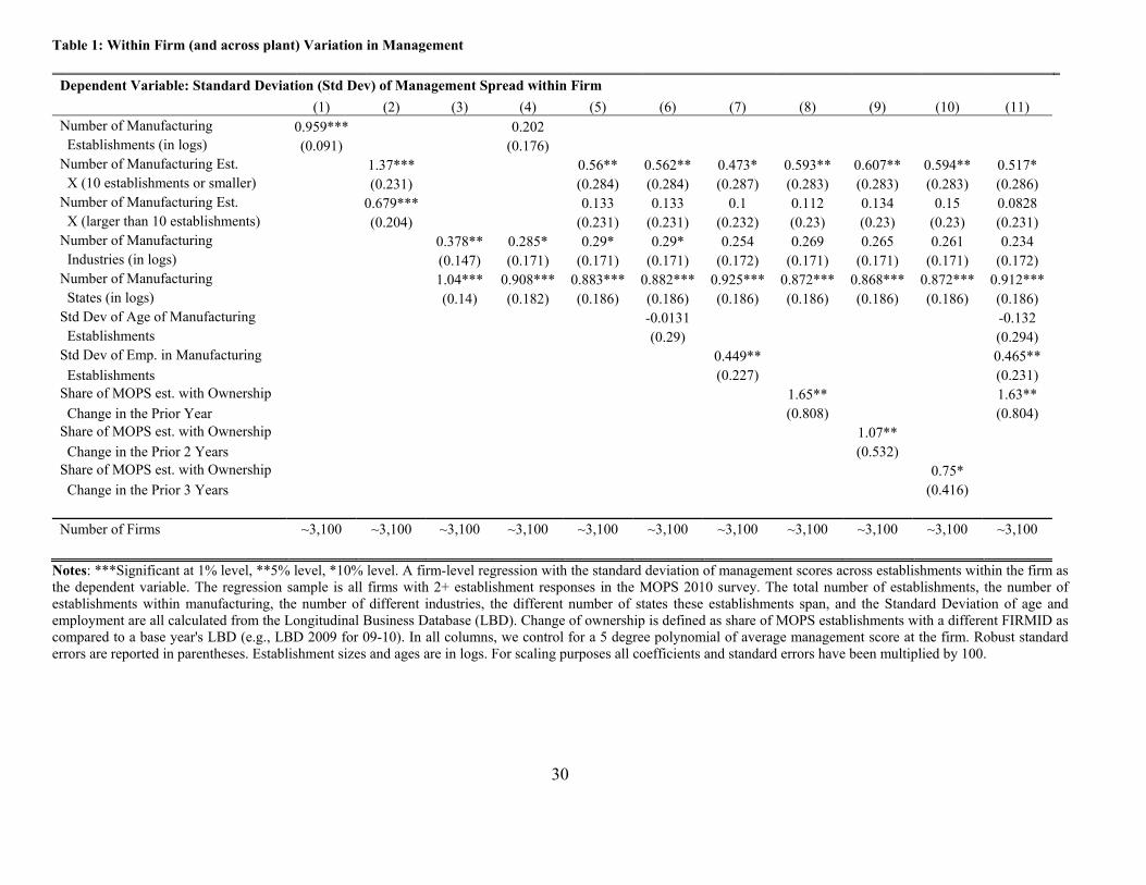
30

Table 1: Within Firm (and across plant) Variation in Management

Dependent Variable: Standard Deviation (Std Dev) of Management Spread within Firm

(1) (2) (3) (4) (5) (6) (7) (8) (9) (10) (11) Number of Manufacturing 0.959*** 0.202 Establishments (in logs) (0.091) (0.176) Number of Manufacturing Est. 1.37*** 0.56** 0.562** 0.473* 0.593** 0.607** 0.594** 0.517* X (10 establishments or smaller) (0.231) (0.284) (0.284) (0.287) (0.283) (0.283) (0.283) (0.286) Number of Manufacturing Est. 0.679*** 0.133 0.133 0.1 0.112 0.134 0.15 0.0828 X (larger than 10 establishments) (0.204) (0.231) (0.231) (0.232) (0.23) (0.23) (0.23) (0.231) Number of Manufacturing 0.378** 0.285* 0.29* 0.29* 0.254 0.269 0.265 0.261 0.234 Industries (in logs) (0.147) (0.171) (0.171) (0.171) (0.172) (0.171) (0.171) (0.171) (0.172) Number of Manufacturing 1.04*** 0.908*** 0.883*** 0.882*** 0.925*** 0.872*** 0.868*** 0.872*** 0.912*** States (in logs) (0.14) (0.182) (0.186) (0.186) (0.186) (0.186) (0.186) (0.186) (0.186) Std Dev of Age of Manufacturing -0.0131 -0.132 Establishments (0.29) (0.294) Std Dev of Emp. in Manufacturing 0.449** 0.465** Establishments (0.227) (0.231) Share of MOPS est. with Ownership 1.65** 1.63** Change in the Prior Year (0.808) (0.804) Share of MOPS est. with Ownership 1.07** Change in the Prior 2 Years (0.532) Share of MOPS est. with Ownership 0.75* Change in the Prior 3 Years (0.416) Number of Firms ~3,100 ~3,100 ~3,100 ~3,100 ~3,100 ~3,100 ~3,100 ~3,100 ~3,100 ~3,100 ~3,100

Notes: ***Significant at 1% level, **5% level, *10% level. A firm-level regression with the standard deviation of management scores across establishments within the firm as the dependent variable. The regression sample is all firms with 2+ establishment responses in the MOPS 2010 survey. The total number of establishments, the number of establishments within manufacturing, the number of different industries, the different number of states these establishments span, and the Standard Deviation of age and employment are all calculated from the Longitudinal Business Database (LBD). Change of ownership is defined as share of MOPS establishments with a different FIRMID as compared to a base year's LBD (e.g., LBD 2009 for 09-10). In all columns, we control for a 5 degree polynomial of average management score at the firm. Robust standard errors are reported in parentheses. Establishment sizes and ages are in logs. For scaling purposes all coefficients and standard errors have been multiplied by 100.

31

Table 2: Plant Management Scores and Performance

Notes: ***Significant at 1% level, **5% level, *10% level. OLS coefficients with standard errors in parentheses (clustered at the firm level). The management score is the unweighted average of the score for each of the 16 questions, where each question is first normalized to be on a 0-1 scale. The sample in all columns is all MOPS observations with at least 11 non-missing responses to management questions and a successful match to ASM, which were also included in ASM tabulations, have positive value added, positive employment and positive imputed capital in the ASM. In columns (1) through (4) the dependent variable is log(real value added over total employment). In columns (5) to (6) the dependent variable is employment growth between 2010 and 2013. Growth is calculated as 0.5*(e2013- e2010)/ (e2013+e2010). In columns (7) to (8) the dependent variable is a dummy that takes the value of 1 for exit between 2010 and 2013. In columns (5)-(8), both TFP and management are normalized by their standard deviation for easier comparison of their association with growth and exit. In column (9) profits are measured by value added minus wages and salaries over total value of shipments. Dependent variable in column (10) is log(1+(R&D per 1000 employees)) from BRDIS. When we include establishment fixed effects, we pool the years 2005 and 2010, with a dummy for 2010. Noise controls include: the absolute difference in reported employment in the ASM and MOPS; a dummy for whether filing was online (zero if by mail); filing date; day of week; respondent tenure and seniority.

Dependent Variable Log(VA/Emp) Emp. Growth

2010-2013 Exit

2010 to 2013 Profit/Sales

R&D/ Emp

(1) (2) (3) (4) (5) (6) (7) (8) (9) (10) Management 1.272*** 0.498*** 0.298*** 0.233*** 0.056*** 0.052*** -0.019*** -0.018*** 0.058*** 0.385*** (0.05) (0.037) (0.065) (0.082) 0.005 0.005 0.002 0.002 (0.01) (0.104) Log(Capital/Emp) 0.179*** 0.036* 0.193*** 0.01*** 0.12***

(0.007) (0.02) (0.016) (0.002) (0.016)

Log(Emp) -0.035*** -0.198*** -0.064*** 0.001 0.102*** (0.006) (0.029) (0.012) (0.002) (0.014) Share employees w. 0.418*** -0.096 0.421*** 0.004 1.008*** a college degree (0.041) (0.138) (0.076) (0.011) (0.09) Productivity (TFP) 0.033*** -0.009*** 0.005 0.002

Observations 31,793 31,793 35,688 17,235 31,793 31,793 31,793 31,793 31,793 13,888

Num. establishments 31,793 31,793 17,844 17,235 31,793 31,793 31,793 31,793 17,843 4,914

Num. firms (clusters) 17,843 17,843 10,557 3,285 17,843 17,843 17,843 17,843 17,843 4,914

Fixed Effects None Industry Establish. Firm Industry Industry Industry Industry Industry Industry

32

Table 3: Drivers of TFP Variation (1) (2) (3) (4) (5) Dependent Variable: Revenue-based Total Factor Productivity Management score 0.684*** 0.495*** (0.040) (0.041) R&D 0.098*** 0.073*** (0.009) (0.009) IT/worker 0.015*** 0.008*** (0.003) (0.002) Skills (% employees 0.527*** 0.126** with college degree) (0.060) (0.057) Observations 17,843 17,843 17,843 17,843 17,843 Share of 90-10 explained 0.181 0.169 0.0752 0.111 0.325 Notes: OLS coefficients with standard errors in parentheses (clustered at the firm level). Dependent variable is firm level TFP built from industry de-meaned plant-level TFP weighted up by plant’s shipments. Right-hand side variables are management score, R&D from BRDIS measured aslog(1+R&D intensity) where R&D intensity is the total domestic R&D expenditure divided by total domestic employment, IT investment perworker (1000*investment in computers per employee), skill measured by the share of employees (managers and non-managers) with a collegedegree. All these variables are also weighted up to the firm level using plant’s total value of shipments. Missing values have been replaced byzero for R&D and by means for the other variables. Industry demeaning is at NAICS 6 level. All regressions are weighted by the number ofestablishments in the firm. “Share of 90-10 explained” is calculated by multiplying the coefficient on the key driver variable (e.g., managementin column 1) by its 90-10 spread and dividing this by the 90-10 spread of TFP.

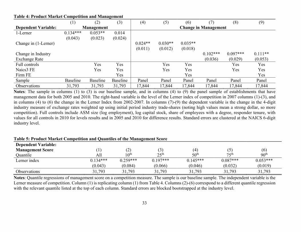
33

Table 4: Product Market Competition and Management (1) (2) (3) (4) (5) (6) (7) (8) (9) Dependent Variable: Management Change in Management 1-Lerner 0.134*** 0.053** 0.014 (0.043) (0.023) (0.024) Change in (1-Lerner) 0.024** 0.030** 0.035** (0.011) (0.012) (0.018) Change in Industry 0.102*** 0.097*** 0.111** Exchange Rate (0.036) (0.029) (0.053) Full controls Yes Yes Yes Yes Yes Yes Naics3 FE Yes Yes Yes Yes Yes Yes Firm FE Yes Yes Yes Sample Baseline Baseline Baseline Panel Panel Panel Panel Panel Panel Observations 31,793 31,793 31,793 17,844 17,844 17,844 17,844 17,844 17,844

Notes: The sample in columns (1) to (3) is our baseline sample, and in columns (4) to (9) the panel sample of establishments that have management data for both 2005 and 2010. The right-hand variable is the level of the Lerner index of competition in 2007 columns (1)-(3), and in columns (4) to (6) the change in the Lerner Index from 2002-2007. In columns (7)-(9) the dependent variable is the change in the 4-digit industry measure of exchange rates weighted up using initial period industry trade-shares (noting high values mean a strong dollar, so more competition). Full controls include ASM size (log employment), log capital stock, share of employees with a degree, responder tenure, with values for all controls in 2010 for levels results and in 2005 and 2010 for difference results. Standard errors are clustered at the NAICS 6-digit industry level. Table 5: Product Market Competition and Quantiles of the Management Score Dependent Variable: Management Score (1) (2) (3) (4) (5) (6) Quantile All 10th 25th 50th 75th 90th Lerner index 0.134*** 0.259*** 0.197*** 0.145*** 0.087*** 0.053***

(0.043) (0.084) (0.066) (0.046) (0.032) (0.019) Observations 31,793 31,793 31,793 31,793 31,793 31,793

Notes: Quantile regressions of management score on a competition measure. The sample is our baseline sample. The independent variable is the Lerner measure of competition. Column (1) is replicating column (1) from Table 4. Columns (2)-(6) correspond to a different quantile regression with the relevant quantile listed at the top of each column. Standard errors are blocked bootstrapped at the industry level.

34

Table 6: Management and the Business Environment

Dependent Variable Management Score Promotions and

Dismissals

All but Promotions and

Dismissals (1) (2) (3) (4) (5) (6) RTW state 0.014** 0.022*** 0.031*** 0.008 (0.006) (0.008) (0.007) (0.006) Oldest in RTW state 0.027***

(0.002)

HQ in RTW state 0.015***

(0.003)

Establishments: 5,143 2,929 16,280 16,280 5,143 5,143 Distance from border: <=50km <=50km All All <=50km <=50km

Sample All Non-

Tradable Multi-Unit Multi-Unit All All

Border FE Yes Yes n/a n/a Yes Yes State FE n/a n/a Yes Yes n/a n/a

Note: Observations in columns (1), (2), (5) and (6) are establishment-border combinations across “Right To Work” (RTW) and Non-RTW (NRTW) borders. Non-Tradables are the 118 industry categories (out of 472) with the lowest regional concentration level calculated following Ellison and Glaeser (1997) using data from the 2007 census. Columns (3) and (4) sample includes all establishment in multi-unit firms with at least one establishment in a RTW and one-establishment in a NRTW state. We consider a firm to have a RTW headquarter if it has at least one establishment in the Longitudinal Business Database (LBD) with NAICS code 551114 "corporate, subsidiary and regional managing offices” located in a RTW state. If no establishment in the firm has this NAICS code, we instead define the headquarters as the oldest establishment in the firm. Standard errors in columns (1) and (2) are calculated using the establishment-border data and are clustered at the border level, while standard errors in columns (3) and (4) are clustered at the firm level. All specifications include industry fixed-effects.

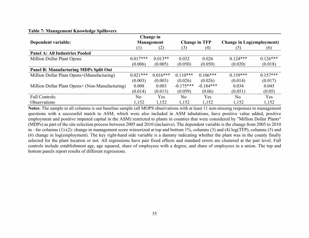
35

Table 7: Management Knowledge Spillovers

Dependent variable: Change in

Management Change in TFP Change in Log(employment) (1) (2) (3) (4) (5) (6) Panel A: All Industries Pooled Million Dollar Plant Opens 0.017*** 0.013** 0.032 0.026 0.124*** 0.126*** (0.006) (0.005) (0.050) (0.050) (0.020) (0.018) Panel B: Manufacturing MDPs Split Out Million Dollar Plant Opens×(Manufacturing) 0.021*** 0.016*** 0.110*** 0.106*** 0.159*** 0.157*** (0.003) (0.003) (0.026) (0.026) (0.014) (0.017) Million Dollar Plant Opens× (Non-Manufacturing) 0.008 0.003 -0.175*** -0.184*** 0.034 0.045 (0.014) (0.013) (0.059) (0.06) (0.051) (0.05) Full Controls: No Yes No Yes No Yes Observations 1,152 1,152 1,152 1,152 1,152 1,152

Notes: The sample in all columns is our baseline sample (all MOPS observations with at least 11 non-missing responses to management questions with a successful match to ASM, which were also included in ASM tabulations, have positive value added, positive employment and positive imputed capital in the ASM) restricted to plants in counties that were considered by "Million Dollar Plants" (MDPs) as part of the site selection process between 2005 and 2010 (inclusive). The dependent variable is the change from 2005 to 2010 in - for columns (1)-(2): change in management score winsorized at top and bottom 1%, columns (3) and (4) log(TFP), columns (5) and (6) change in log(employment). The key right-hand side variable is a dummy indicating whether the plant was in the county finally selected for the plant location or not. All regressions have pair fixed effects and standard errors are clustered at the pair level. Full controls include establishment age, age squared, share of employees with a degree, and share of employees in a union. The top and bottom panels report results of different regressions.

36

Table 8: Management and Education Dependent Variable: Management Score (1) (2) (3) (4) Specification OLS OLS OLS IV Land Grant in MSA^ 0.528** 0.418* (0.211) (0.254) Share in county with BA+

0.037*** 0.133** (0.012) (0.054)

1st stage F-stat 31.42 Firm FE No Yes No No Observations 31,793 17,235 31,793 31,793

Notes: Regressions of the combined management score on measures of local skill levels. Columns (1)-(3) are OLS regressions while in column (4) we instrument Share in county with BA or above with the presence of a Land Grant College (LGC). All columns have area level controls for population density and the unemployment rate as well as industry and state fixed effects. Establishment-level controls include log(employment), log(age), multi-unit dummy, exporter dummy, and union share. High skill and low skill industries are above and below median industries using the degree variable in our sample. Coefficient and standard error on Land Grand Colleges multiplied by 100. Standard errors clustered at the MSA. Table 9: Quantification of Management Drivers Driver 90-10 Coefficient Implied 90-10 Implied share of true management 90-10 Competition 0.25 0.053 0.013 6.3% Business Regulation 1 0.022 0.022 10.5% Spillovers (Million Dollar Plants) 1 0.013 0.013 6.2% Education 0.25 0.133 0.033 15.7% Total 38.7%

Notes: “Driver 90-10” is the 90-10 spread of the variable in the data (for competition and education - this comes from estimates from Compustat and the ACS since we cannot clear out sample values). “Coefficient’” is our regression coefficient from our preferred regression result for that driver – which for competition, business regulation, spillovers and education is column (2) Table 4, column (3) Table 6, column (2) Table 7, and column (6) Table 8, respectively. The “Implied 90-10” is column (1) multiplied by column (2). Finally, “Implied share of true management 90-10” is the implied 90-10 from column (3) as a percentage of 0.210, which is our calculated true management 90-10. This value of 0.210 comes from the measured management 90-10 (which is 0.385, as shown in Table A2) multiplied by the 0.546 (the share of this variation that is real rather than measurement error, as discussed in Section 3).

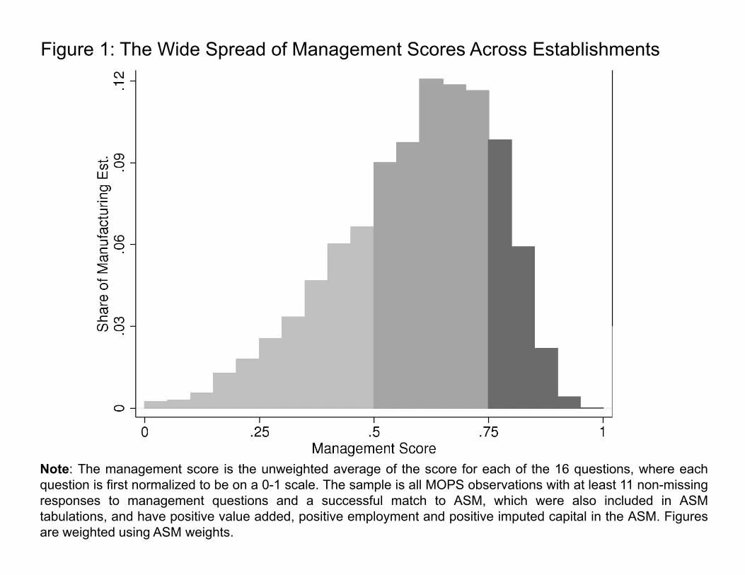
Figure 1: The Wide Spread of Management Scores Across Establishments

Note: The management score is the unweighted average of the score for each of the 16 questions, where eachquestion is first normalized to be on a 0-1 scale. The sample is all MOPS observations with at least 11 non-missingresponses to management questions and a successful match to ASM, which were also included in ASMtabulations, and have positive value added, positive employment and positive imputed capital in the ASM. Figuresare weighted using ASM weights.

Man

agem

ent sprea

d accoun

ted for b

y firm

Number of establishments in the firm

Figure 2: The firm-level share of the variation in management scores (after removing measurement error)

Note: Dots show the share of management score variation accounted for by the firm with different numbers of manufacturingestablishments ranging from that number to the next value – so for example, 50 plants refers to 50 to 74 plants. After removing the45.4% accounted for by measurement error. The bootstrap sampled 95% confidence interview shown in grey shading. Sample of16,500 establishments across the 3100 firms with 2+ establishments in the 2010 MOPS survey.

Management, removing within firm industry and geo variation

Management

Number of establishments in the firm

Figure 3: The distribution of the management regression coefficient over 86 NAICS four-digit industries

Note: Smoothed density of the management coefficient from running the regression in column (2) of Table 2 separately for each of the86 four-digit manufacturing NAICS codes. The sample of 31,793 is all MOPS observations with at least 11 non-missing responses tomanagement questions and a successful match to ASM, which were also included in ASM tabulations, have positive value added,positive employment and positive imputed capital in the ASM.

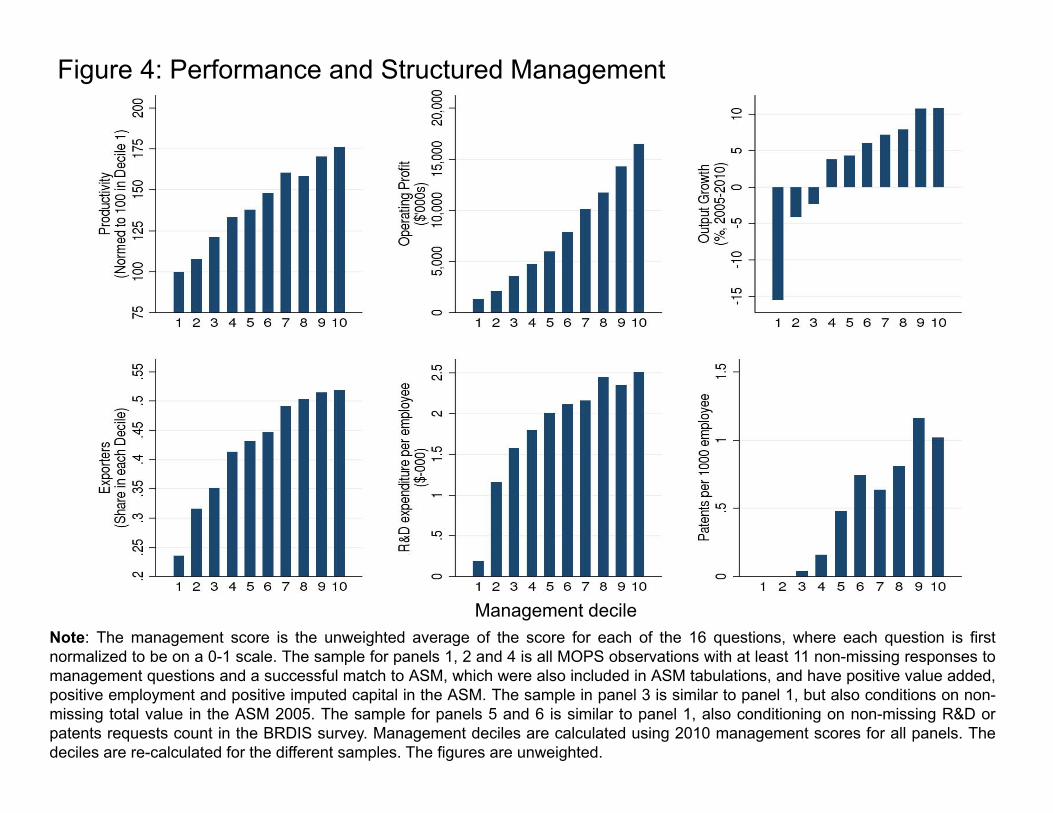
Figure 4: Performance and Structured Management

Note: The management score is the unweighted average of the score for each of the 16 questions, where each question is firstnormalized to be on a 0-1 scale. The sample for panels 1, 2 and 4 is all MOPS observations with at least 11 non-missing responses tomanagement questions and a successful match to ASM, which were also included in ASM tabulations, and have positive value added,positive employment and positive imputed capital in the ASM. The sample in panel 3 is similar to panel 1, but also conditions on non-missing total value in the ASM 2005. The sample for panels 5 and 6 is similar to panel 1, also conditioning on non-missing R&D orpatents requests count in the BRDIS survey. Management deciles are calculated using 2010 management scores for all panels. Thedeciles are re-calculated for the different samples. The figures are unweighted.

Management decile